2010 rams doe and data analysis
DESCRIPTION
Edit_5TRANSCRIPT

Copyright © 2010 IEEE. Reprinted from “2010 Reliability and Maintainability Symposium,” San Jose, CA, USA, January 25-28, 2010. This material is posted here with permission of the IEEE. Such permission of the IEEE does not in any way imply IEEE endorsement of any of ReliaSoft Corporation's products or services. Internal or personal use of this material is permitted. However, permission to reprint/republish this material for advertising or promotional purposes or for creating new collective works for resale or redistribution must be obtained from the IEEE by writing to [email protected]. By choosing to view this document, you agree to all provisions of the copyright laws protecting it.

Tutorial Notes © 2010 AR&MS
2010 Annual RELIABILITY and MAINTAINABILITY Symposium
Design of Experiments and Data Analysis
Huairui Guo, Ph. D. & Adamantios Mettas
Huairui Guo, Ph.D., CPR. Adamantios Mettas, CPR ReliaSoft Corporation ReliaSoft Corporation 1450 S. Eastside Loop 1450 S. Eastside Loop Tucson, AZ 85710 USA Tucson, AZ 85710 USA e-mail: [email protected] e-mail: [email protected]

ii – Guo & Mettas 2010 AR&MS Tutorial Notes
SUMMARY & PURPOSE
Design of Experiments (DOE) is one of the most useful statistical tools in product design and testing. While many organizations benefit from designed experiments, others are getting data with little useful information and wasting resources because of experiments that have not been carefully designed. Design of Experiments can be applied in many areas including but not limited to: design comparisons, variable identification, design optimization, process control and product performance prediction. Different design types in DOE have been developed for different purposes. Many engineers are confused or even intimidated by so many options.
This tutorial will focus on how to plan experiments effectively and how to analyze data correctly. Practical and correct methods for analyzing data from life testing will also be provided.
Huairui Guo, Ph.D., CRP Huairui Guo is the Director of Theoretical Development at ReliaSoft Corporation. He received his Ph.D. in Systems and Industrial Engineering from the University of Arizona. He has published numerous papers in the areas of quality engineering including SPC, ANOVA and DOE and reliability engineering. His current research interests include repairable system modeling, accelerated life/degradation Testing, warranty data analysis and robust optimization. Dr. Guo is a member of SRE, IIE and IEEE. He is a Certified Reliability Professional (CRP).
Adamantios Mettas, CRP Mr. Mettas is the Vice President of product development at ReliaSoft Corporation. He fills a critical role in the advancement of ReliaSoft's theoretical research efforts and formulations in the subjects of Life Data Analysis, Accelerated Life Testing, and System Reliability and Maintainability. He has played a key role in the development of ReliaSoft's software including, Weibull++, ALTA and BlockSim, and has published numerous papers on various reliability methods. Mr. Mettas holds a B.S degree in Mechanical Engineering and an M.S. degree in Reliability Engineering from the University of Arizona. He is a Certified Reliability Professional (CRP).
Table of Contents 1. Introduction ..........................................................................................................................................................................1 2. Statistical Background ..........................................................................................................................................................2 3. Two Level Factorial Design .................................................................................................................................................3 4. Response Surface Methods (RSM) ......................................................................................................................................6 5. DOE for Life Testing ...........................................................................................................................................................9 6. Conclusions ........................................................................................................................................................................ 10 7. References .......................................................................................................................................................................... 11 8. Tutorial Visuals…………………………………………………………………………………….. ................................. 12

2010 Annual RELIABILITY and MAINTAINABILITY Symposium Guo & Mettas – 1
1. INTRODUCTION
The most effective way to improve product quality and reliability is to integrate them in the design and manufacturing process. Design of Experiments (DOE) is a useful tool that can be integrated into the early stages of the development cycle. It has been successfully adopted by many industries, including automotive, semiconductor, medical devices, chemical products, etc. The application of DOE is not limited to engineering. Many successful stories can be found in other areas. For example, it has been used to reduce administration costs, improve the efficiency of surgery processes, and establish better advertisement strategies.
1.1 Why DOE
DOE will make your life easier. For many engineers, applying DOE knowledge in their daily work will reduce lots of trouble. Here are two examples of bad experiments that will cause trouble. Example 1: Assume the reliability of a product is affected by voltage. The usage level voltage is 10. In order to predict the reliability at the usage level, fifty units are available for accelerated life testing. An engineer tested all fifty units at a voltage of 25. Is this a good test? Example 2: Assume the reliability of a product is affected by temperature and humidity. The usage level is 40 degrees Celsius and 50% relative humidity. In order to predict the reliability at the usage level, fifty units are available for accelerated life testing. The design is conducted in the following way:
Number of Units
Temperature (Celsius)
Humidity (%)
25 120 95 25 85 85
Table 1 – Two Stress Accelerated Life Test
Will the engineer be able to predict the reliability at the usage level with the failure data from this test?
1.2 What DOE Can Do
DOE can help you design better tests than the above two examples. Based on the objectives of the experiments, DOE can be used for the following purposes [1, 2]: 1. Comparisons. When you have multiple design options, several materials or suppliers are available, you can design an experiment to choose the best one. For example, in the comparison of six different suppliers that provide connectors, will the components have the same expected life? If they are different, how are they different and which is the best? 2. Variable Screening. If there are a large number of variables that can affect the performance of a product or a system, but only a relatively small number of them are important, a screening experiment can be conducted to identify the important variables. For example, the warranty return is abnormally high after a new product is launched.
Variables that may affect the life are temperature, voltage, duty cycle, humidity and several other factors. DOE can be used to quickly identify the troublemakers and a follow-up experiment can provide the guidelines for design modification to improve the reliability. 3. Transfer Function Exploration. Once a small number of variables have been identified as important, their effects on the system performance or response can be further explored. The relationship between the input variables and output response is called the transfer function. DOE can be applied to design efficient experiments to study the linear and quadratic effects of the variables and some of the interactions between the variables. 4. System Optimization. The goal of system design is to improve the system performance, such as to improve the efficiency, quality, and reliability. If the transfer function between variables and responses has been identified, the transfer function can be used for design optimization. DOE provides an intelligent sequential strategy to quickly move the experiment to a region containing the optimum settings of the variables. 5. System Robustness. In addition to optimizing the response, it is important to make the system robust against “noise,” such as environmental factors and uncontrolled factors. Robust design, one of the DOE techniques, can be used to achieve this goal.
1.3 Common Design Types
Different designs have been used for different experiment purposes. The following list gives the commonly used design types.
1. For comparison • One factor design
2. For variable screening • 2 level factorial design • Taguchi orthogonal array • Plackett-Burman design
3. For transfer function identification and optimization • Central composite design • Box-Behnken design
4. For system robustness • Taguchi robust design
The designs used for transfer function identification and optimization are called Response Surface Method designs. In this tutorial, we will focus on 2 level factorial design and response surface method designs. They are the two most popular and basic designs.
1.4 General Guidelines for Conducting DOE
DOE is not only a collection of statistical techniques that enable an engineer to conduct better experiments and analyze data efficiently; it is also a philosophy. In this section, general guidelines for planning efficient experiments will be given. The following seven-step procedure should be followed [1, 2]. 1. Clarify and State Objective. The objective of the experiment should be clearly stated. It is helpful to prepare a

2 – Guo & Mettas 2010 AR&MS Tutorial Notes
list of specific problems that are to be addressed by the experiment. 2. Choose Responses. Responses are the experimental outcomes. An experiment may have multiple responses based on the stated objectives. The responses that have been chosen should be measurable. 3. Choose Factors and Levels. A factor is a variable that is going to be studied through the experiment in order to understand its effect on the responses. Once a factor has been selected, the value range of the factor that will be used in the experiment should be determined. Two or more values within the range need to be used. These values are referred to as levels or settings. Practical constraints of treatments must be considered, especially when safety is involved. A cause-and-effect diagram or a fishbone diagram can be utilized to help identify factors and determine factor levels. 4. Choose Experimental design. According to the objective of the experiments, the analysts will need to select the number of factors, the number of level of factors, and an appropriate design type. For example, if the objective is to identify important factors from many potential factors, a screening design should be used. If the objective is to optimize the response, designs used to establish the factor-response function should be planned. In selecting design types, the available number of test samples should also be considered. 5. Perform the Experiment. A design matrix should be used as a guide for the experiment. This matrix describes the experiment in terms of the actual values of factors and the test sequence of factor combinations. For a hard-to-set factor, its value should be set first. Within each of this factor’s settings, the combinations of other factors should be tested. 6. Analyze the Data. Statistical methods such as regression analysis and ANOVA (Analysis of Variance) are the tools for data analysis. Engineering knowledge should be integrated into the analysis process. Statistical methods cannot prove that a factor has a particular effect. They only provide guidelines for making decisions. Statistical techniques together with good engineering knowledge and common sense will usually lead to sound conclusions. Without common sense, pure statistical models may be misleading. For example, models created by smart Wall Street scientists did not avoid, and probably contributed to, the economic crisis in 2008. 7. Draw Conclusions and Make Recommendations. Once the data have been analyzed, practical conclusions and recommendations should be made. Graphical methods are often useful, particularly in presenting the results to others. Confirmation testing must be performed to validate the conclusion and recommendations.
The above seven steps are the general guidelines for performing an experiment. A successful experiment requires knowledge of the factors, the ranges of these factors and the appropriate number of levels to use. Generally, this information is not perfectly known before the experiment. Therefore, it is suggested to perform experiments iteratively and sequentially. It is usually a major mistake to design a single, large, comprehensive experiment at the start of a study.
As a general rule, no more than 25 percent of the available resources should be invested in the first experiment.
2. STATISTICAL BACKGROUND
Linear regression and ANOVA are the statistical methods used in DOE data analysis. Knowing them will help you have a better understand of DOE.
2.1 Linear Regression[2]
A general linear model or a multiple regression model is: εβββ ++++= pp XXY ...110 (1)
Where: Y is the response also called output or dependent variable. iX is the predictor also called input or independent variable. ε is the random error or noise, which is assumed to be normally distributed with mean 0 and variance 2σ , usually noted as ),0(~ 2σε N . Because ε is normally distributed, then for a given value of X, Y is also normally distributed and
2)( σ=YVar . From the model, it can be seen that the variation or the
difference of Y consists of two parts. One is the random part of ε . The other is the difference caused by the difference of the X values. For example, consider the data in Table 2:
Observation X1 X2 Y Y
Mean
1 120 90 300 325 2 120 90 350
3 85 95 150 170 4 85 95 190
5 120 95 400 415 6 120 95 430
Table 2 – Example Data for Linear Regression
Table 2 has three different combinations of X1 and X2, showing at different colors. For each combination, there are two observations. Because of the randomness caused by ε , these two observations are different although they have the same X values. This difference usually is called within-run variation. The mean values of Y at the three combinations are different too. This difference is caused by the difference of X1 and X2 and usually is called between-run variation.
If the between-run variation is significantly larger than the within-run variation, it means most of the variation of Y is caused by the difference of X settings. In other words, Xs significantly affect Y. The difference of Ys caused by the Xs are much more significant than the difference caused by the noise.
From Table 2, we have the feeling that the between-run variation is larger than the within-run variation. To confirm this, statistical methods should be applied. The amount of the total variation of Y is defined by the sum of squares:
( )∑=
−=n
iiT YYSS
1
2 (2)
Where iY is the ith observed value and Y is the mean of all

2010 Annual RELIABILITY and MAINTAINABILITY Symposium Guo & Mettas – 3
the observations. However, since SST is affected by the number of observations, to eliminate this effect, another metric called mean squares is used to measure the normalized variability of Y.
( )∑=
−−
=−
=n
ii
TT YY
nnSS
MS1
2
11
1 (3)
Equation (3) is also the unbiased estimator of )(YVar . As mentioned before, the total sum of squares can be
partitioned into two parts: within-run variation caused by random noise (called sum of squares of error ESS ) and the between-run variation caused by different values of Xs (called sum of squares of regression RSS ).
∑∑==
−+−=+=n
iii
n
iiERT YYYYSSSSSS
1
2
1
2 )ˆ()ˆ( (4)
Where: iY is the predicted value for the ith test. For tests with the same X values, the predicted values are the same.
Similar to equation (3), the mean squares of regression and the mean squares of error are calculated by:
( )∑=
−==n
ii
RR YY
ppSS
MS1
2ˆ1 (5)
( )∑=
−−−
=−−
=n
iii
EE YY
pnpnSSMS
1
2ˆ11
1 (6)
Where: p is the number of Xs. When there is more than one input variable, RSS can be
further divided into the variation caused by each variable, such as:
pXXXR SSSSSSSS +++= ...21
(7)
The mean squares of each input variable iXMS is compared
with EMS to test if the effect of iX is significantly greater than the effect of noise.
The mean squares of regression RMS is used to measure the between-run variance that is caused by predictor Xs. The mean squares of error EMS represents the within-run variance caused by noise. By comparing these two values, we can find out if the variance contributed by Xs is significantly greater than the variance caused by noise. ANOVA is the method used for the comparison in a statistical way.
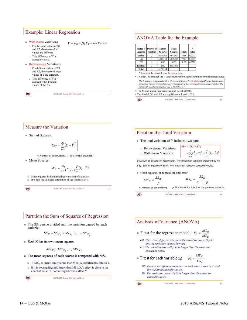
2.2 ANOVA (Analysis of Variance)
The following ratio
E
RMSMSF =0 (8)
is used to test the following two hypotheses: H0: There is no difference between the variance caused
by Xs and the variance caused by noise. H1: The variance caused by Xs is larger than the variance
caused by noise. Under the null hypothesis, the ratio follows the F distribution with degree of freedoms of p and pn −−1 . By applying ANOVA to the data for this example, we get the following ANOVA table. The third column shows the values for the sum of squares. We
can easily verify that: EXXERT SSSSSSSSSSSS ++=+=
21 (9)
The fifth column shows the F ratio of each source. All the values are much bigger than 1. The last column is the P value. The smaller the P value is, the larger the difference between the variance caused by the corresponding source and the variance caused by noise. Usually, a significance level α , such as 0.05 or 0.1 is used to compare with the P values. If a P value is less than α , the corresponding source is said to be significant at the significance level of α . From Table 3, we can see that both variables X1 and X2 are significant to the response Y at the significance level of 0.1.
Source of Variation
Degrees of
Freedom
Sum of Squares
Mean Squares
F Ratio
P Value
Model 2 6.14E+04 3.07E+04 36.86 0.0077
X1 1 6.00E+04 6.00E+04 72.03 0.0034
X2 1 8100 8100 9.72 0.0526
Residual 3 2500 833.3333
Total 5 6.39E+04
Table 3 – ANOVA Table for the Linear Regression Example
Another way to test whether or not a variable is significant is to test whether or not its coefficient is 0 in the regression model. For this example, the linear regression model is:
εβββ +++= 21110 XXY (10) If we want to test whether or not 01 =β , we can use the following hypothesis:
H0: 01 =β Under this null hypothesis, the statistic is a t distribution:
)( 1
10 β
βse
T = (11)
)( 1βSe is the standard error of 1β that is estimated from the data. The t test results are given in Table 4.
Term Coefficient Standard Error T Value P Value
Intercept -2135 588.7624 -3.6263 0.0361 X1 7 0.8248 8.487 0.0034
X2 18 5.7735 3.1177 0.0526
Table 4 – Coefficients for the Linear Regression Example
Table 3 and Table 4 give the same P values. With linear regression and ANOVA in mind, we can start
discussing DOE now.
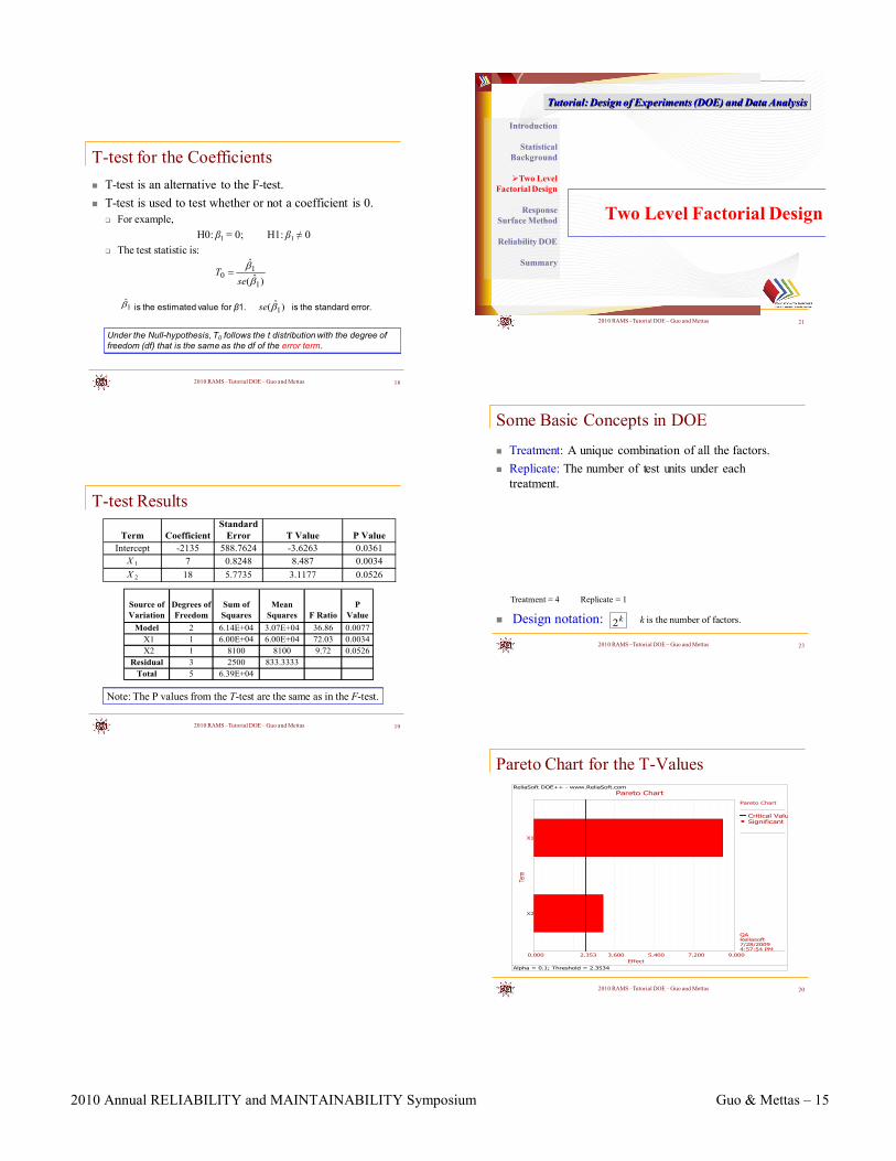
3. TWO LEVEL FACTORIAL DESIGNS
Two level factorial designs are used for factor screening. In order to study the effect of a factor, at least two different settings for this factor are required. This also can be explained from the viewpoint of linear regression. To fit a line, two points are the minimal requirement. Therefore, the engineer

4 – Guo & Mettas 2010 AR&MS Tutorial Notes
who tested all the units at a voltage of 25 will not be able to predict the life at the usage level of 10 volts. With only one voltage value, the effect of voltage cannot be evaluated.
3.1 Two Level Full Factorial Design
When the number of factors is small and you have the resources, a full factorial design should be conducted. Here we will use a simple example to introduce some basic concepts in DOE.
For an experiment with two factors, the factors usually are called A and B. Uppercase letters are used for factors. The first level or the low level is represented by -1, while the second level or the high level is represented by 1. There are four combinations of a 2 level 2 factorial design. Each combination is called a treatment. Treatments are represented by lowercase letters. The number of test units for each treatment is called the number of replicates. For example, if you test two samples at each treatment, the number of replicates is 2. Since the number of replicates for each factor combination is the same, this design is also balanced. A two level factorial design with k factors usually is written as k2 design and read as “2 to the power of 3 design” or “2 to the 3 design.” For a 22 design, the design matrix is:
Treatment Factors
Response A B
-1 -1 -1 20
a 1 -1 30
b -1 1 25
ab 1 1 35
Table 5 – Treatments for 2 Level Factorial Design
This design is orthogonal. This is because the sum of the product of A and B is zero, which is
0)11()11()11()11( =×+×−+−×+−×− . An orthogonal design will reduce the estimation uncertainty of the model coefficients.
The following linear regression model is used for the analysis:
εββββ ++++= 211222110 XXXXY (12) Where: 1X is for factor A; 2X is for factor B; and their interaction is represented by 21XX . The effects of A and B are called main effects. The effects of their interaction are called two-way interaction effects. These three effects are the three sources for the variation of Y. Since equation (12) is a linear regression model, the ANOVA method and the t-test given in Section 2 can be used to test whether or not one effect is significant.
For a balanced design, a simple way to calculate the effect of a factor is to calculate the difference of the mean values of the response at its high and low setting. For example, the effect of A can be calculated by:
102
25202
3530
Aat Avg. - Aat Avg. A ofEffet lowhigh
=+
−+
=
= (13)
3.2 Two Level Fractional Factorial Design
When you increase the number of factors, the number of test units will increase quickly. For example, to study 7 factors, 128 units are needed. In reality, responses are affected by a small number of main effects and lower order interactions. Higher order interactions are relatively unimportant. This statement is called the sparsity of effects principle. According to this principle, fractional factorial designs are developed. These designs use fewer samples to estimate main effects and lower order interactions, while the higher order interactions are considered to have negligible effects.
Consider a 32 design. 8 test units are required for a full factorial design. Assume only 4 test units are available because of the cost of the test. Which 4 of the 8 treatments should you choose? A full design matrix with all the effects for a 32 design is:
Order A B AB C AC BC ABC
1 -1 -1 1 -1 1 1 -1
2 1 -1 -1 -1 -1 1 1
3 -1 1 -1 -1 1 -1 1 4 1 1 1 -1 -1 -1 -1
5 -1 -1 1 1 -1 -1 1
6 1 -1 -1 1 1 -1 -1
7 -1 1 -1 1 -1 1 -1
8 1 1 1 1 1 1 1
Table 6 – Design Matrix for a 32 Design
If the effect of ABC can be ignored, the following 4 treatments can be used in the experiment.
Order A B AB C AC BC ABC 2 1 -1 -1 -1 -1 1 1 3 -1 1 -1 -1 1 -1 1
5 -1 -1 1 1 -1 -1 1 8 1 1 1 1 1 1 1
Table 7 –Fraction of the Design Matrix for a 32 Design
In Table 7, the effect of ABC cannot be estimated from the experiment because it is always at the same level of 1. Since
Table 7 uses only half of the treatments from the full factorial design in Table 6, it is represented by 132 − and read as “2 to
the power of 3 minus 1 design” or “2 to the 3 minus 1 design.” From Table 7, you will also notice that some columns
have the same values. For example, column AB and C are the same. Using equation (13) to calculate the effect of AB and C, we will end up with the same procedure and result. Therefore, from this experiment, the effect of AB and C cannot be

2010 Annual RELIABILITY and MAINTAINABILITY Symposium Guo & Mettas – 5
distinguished because they change with the same pattern. In DOE, effects that cannot be separated from an experiment are called confounded effects or aliased effects. A list of aliased effects is called the alias structure. For the design of Table 7, the alias structure is:
[I]=I+ABC; [A]=A+AC; [B]=B+BC; [C]=C+AB Where: I is the effect of the intercept in the regression model, which represents the mean value of the response. The alias for I is called the defining relation. For this example, the defining relation is written as I = ABC. In a design, I may be aliased with several effects. The order of the shortest effects that aliased with I is the “resolution” of this design.
From the alias structure, we can see that main effects are confounded with 2-way interactions. For example, the estimated effect for C in fact is the combination effect of C and AB.
Checking Table 7, we can see it is a full factorial design if we have only factor A and B. Therefore, A and B usually are called basic factors and the full factorial design for them is called the basic design. A fractional factorial design is generated from its basic design and basic factor. For this example, the values for factor C are generated from the values of the basic factors A and B using the relation C=AB. Usually AB is called the factor generator for C.
By now, it should be clear that the design given in Table 1 at the beginning of this tutorial is not a good design. If you check the design in terms of coded value, the answer is obvious. Table 8 shows the design again.
Number of
Units Temperature
(Celsius) Humidity
(%) 25 120 (1) 95 (1) 25 85 (-1) 85 (-1)
Table 8 – Two Stress Accelerated Life Test (Coded Value)
In this design, temperature and humidity are confounded. In fact, to study the effect of two factors, at least three different settings are required. From the linear regression point of view, at least three unique settings are needed to solve three parameters: the intercept, the effect of factor A and the effect of factor B. If their interaction is also to be estimated, four different settings should be used. Many DOE software packages can generate a design matrix for you according to the number of factors and the level of factors. It will help you avoid bad designs such as the one given in Table 8.
3.3 An Example of a Fractional Factorial Design
Assume an engineer wants to identify the factors that affect the yield of a manufacturing process for integrated circuits. By following the DOE guidelines, five factors are brought up and a two level fractional factorial design is decided to be used [1]. The five factors and their levels are given in Table 9.
Factor Name Unit Low
(-1) High (1)
A Aperture Setting small large B Exposure Time minutes 20 40 C Develop Time seconds 30 45
D Mask Dimension small large E Etch Time minutes 14.5 15.5
Table 9 –Factor Settings for a Five Factor Experiment
With five factors the total number of runs required for a full factorial is 3225 = . Running all of the 32 combinations is too expensive for the manufacturer. At the initial investigation, only main effects and two factor interactions are of interest, while higher order interactions are considered to be unimportant. It is decided to carry out the investigation using the 152 − design, which requires 16 runs. The defining relation is I=ABCDE, or in other words, the generator for factor E is E=ABCD. Table 10 gives the experiment data.
Run Order A B C D E Yield
1 Large 20 30 Large 15.5 10 2 Large 20 45 Large 14.5 21 3 Small 40 45 Small 15.5 45 4 Small 20 45 Small 14.5 16 5 Large 40 30 Small 15.5 52 6 Large 40 45 Small 14.5 60 7 Small 40 30 Large 15.5 30 8 Small 20 45 Large 15.5 15 9 Large 20 30 Small 14.5 9
10 Small 40 30 Small 14.5 34 11 Small 20 30 Small 15.5 8 12 Large 40 30 Large 14.5 50 13 Small 40 45 Large 14.5 44 14 Small 20 30 Large 14.5 6 15 Large 20 45 Small 15.5 22 16 Large 40 45 Large 15.5 63
Table 10 –Design Matrix and Results
Since the design has only 16 unique factor combinations, it can be used to estimate only 16 parameters in the linear regression model. If we include all main and 2-way interactions in the model, we get the following ANOVA table.
Source of Variation DF Sum of
Squares Mean
Squares F P Value
Model 15 5775.4375 385.0292 - - A 1 495.0625 495.0625 - - B 1 4590.0625 4590.0625 - - C 1 473.0625 473.0625 - - D 1 3.0625 3.0625 - - E 1 1.5625 1.5625 - -
AB 1 189.0625 189.0625 - - AC 1 0.5625 0.5625 - - AD 1 5.0625 5.0625 - -
6 – Guo & Mettas 2010 AR&MS Tutorial Notes
AE 1 5.0625 5.0625 - - BC 1 1.5625 1.5625 - - BD 1 0.0625 0.0625 - - BE 1 0.0625 0.0625 - - CD 1 3.0625 3.0625 - - CE 1 0.5625 0.5625 - - DE 1 7.5625 7.5625 - -
Residual 0 Total 15 5775.4375
Table 11 –ANOVA Table with All Effects
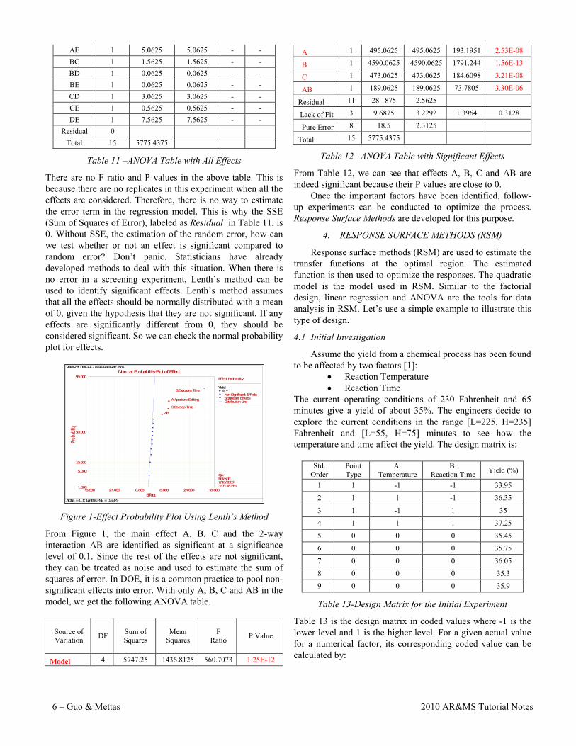
There are no F ratio and P values in the above table. This is because there are no replicates in this experiment when all the effects are considered. Therefore, there is no way to estimate the error term in the regression model. This is why the SSE (Sum of Squares of Error), labeled as Residual in Table 11, is 0. Without SSE, the estimation of the random error, how can we test whether or not an effect is significant compared to random error? Don’t panic. Statisticians have already developed methods to deal with this situation. When there is no error in a screening experiment, Lenth’s method can be used to identify significant effects. Lenth’s method assumes that all the effects should be normally distributed with a mean of 0, given the hypothesis that they are not significant. If any effects are significantly different from 0, they should be considered significant. So we can check the normal probability plot for effects.
Figure 1-Effect Probability Plot Using Lenth’s Method
From Figure 1, the main effect A, B, C and the 2-way interaction AB are identified as significant at a significance level of 0.1. Since the rest of the effects are not significant, they can be treated as noise and used to estimate the sum of squares of error. In DOE, it is a common practice to pool non-significant effects into error. With only A, B, C and AB in the model, we get the following ANOVA table.
Source of Variation DF Sum of
Squares Mean
Squares F
Ratio P Value
Model 4 5747.25 1436.8125 560.7073 1.25E-12
A 1 495.0625 495.0625 193.1951 2.53E-08
B 1 4590.0625 4590.0625 1791.244 1.56E-13
C 1 473.0625 473.0625 184.6098 3.21E-08
AB 1 189.0625 189.0625 73.7805 3.30E-06
Residual 11 28.1875 2.5625
Lack of Fit 3 9.6875 3.2292 1.3964 0.3128
Pure Error 8 18.5 2.3125
Total 15 5775.4375
Table 12 –ANOVA Table with Significant Effects
From Table 12, we can see that effects A, B, C and AB are indeed significant because their P values are close to 0.
Once the important factors have been identified, follow-up experiments can be conducted to optimize the process. Response Surface Methods are developed for this purpose.
4. RESPONSE SURFACE METHODS (RSM)
Response surface methods (RSM) are used to estimate the transfer functions at the optimal region. The estimated function is then used to optimize the responses. The quadratic model is the model used in RSM. Similar to the factorial design, linear regression and ANOVA are the tools for data analysis in RSM. Let’s use a simple example to illustrate this type of design.
4.1 Initial Investigation
Assume the yield from a chemical process has been found to be affected by two factors [1]:
• Reaction Temperature • Reaction Time
The current operating conditions of 230 Fahrenheit and 65 minutes give a yield of about 35%. The engineers decide to explore the current conditions in the range [L=225, H=235] Fahrenheit and [L=55, H=75] minutes to see how the temperature and time affect the yield. The design matrix is:
Std. Order
Point Type
A: Temperature
B: Reaction Time Yield (%)
1 1 -1 -1 33.95
2 1 1 -1 36.35
3 1 -1 1 35
4 1 1 1 37.25
5 0 0 0 35.45
6 0 0 0 35.75
7 0 0 0 36.05
8 0 0 0 35.3
9 0 0 0 35.9
Table 13-Design Matrix for the Initial Experiment
Table 13 is the design matrix in coded values where -1 is the lower level and 1 is the higher level. For a given actual value for a numerical factor, its corresponding coded value can be calculated by:
ReliaSoft DOE++ - www.ReliaSoft.comNormal Probability Plot of Effect
Alpha = 0.1; Lenth's PSE = 0.9375
Effect
Prob
ability
-40.000 40.000-24.000 -8.000 8.000 24.0001.000
5.000
10.000
50.000
99.000
AB
C:Develop Time
A:Aperture Setting
B:Exposure Time
Effect Probability
YieldY' = Y
Non-Significant EffectsSignificant EffectsDistribution Line
QAReliasoft7/10/20093:03:18 PM

2010 Annual RELIABILITY and MAINTAINABILITY Symposium Guo & Mettas – 7
Low andHigh Between Range theof HalfLow andHigh of Value Middle-Value Actual valueCoded = (13)
In Table 13, there are several replicated runs at the setting of (0, 0). These runs are called center points. Center points have the following two uses.
• To estimate random error. • To check whether or not the curvature is significant.
At least five center points are suggested in an experiment. When we analyze the data in Table 13, we get the
ANOVA table below. From Table 14, we know curvature is not significant. Therefore, the linear model is sufficient in the current experiment space. The linear model that includes only significant effects is:
21 4875.01625.16375.35 XXY ++= (14) Equation (14) is in terms of coded value. We can see both factors have a positive effect to the yield since their coefficients are positive. To improve the yield, we should explore the region with factor values larger than the current operation condition. There are many directions we can move to increase the yield, but which one is the fastest lane to approach the optimal region? By checking the coefficient of each factor in equation (14), we know the direction should be (1.1625, 0.4875). This also can be seen from the contour plot in Figure 2.
Source of Variation DF Sum of
Squares Mean
Squares F Ratio P Value
Model 4 6.368 1.592 16.4548 0.0095
A 1 5.4056 5.4056 55.8721 0.0017
B 1 0.9506 0.9506 9.8256 0.035
AB 1 0.0056 0.0056 0.0581 0.8213
Curvature 1 0.0061 0.0061 0.0633 0.8137
Residual 4 0.387 0.0967
Total 8 6.755
Table 14-ANOVA Table for the Initial Experiment
Figure 2--Contour Plot of the Initial Experiment
Step Factor Levels
Yield (%) Coded Actual
A B A B Current Operation 0 0 230 65 35
1 2.4 1 242 75 36.5
2 4.8 2 254 85 39.35 3 7.2 3 266 95 45.65 4 9.6 4 278 105 49.55
5 12 5 290 115 55.7 6 14.4 6 302 125 64.25
7 16.8 7 314 135 72.5 8 19.2 8 326 145 80.6
9 21.6 9 338 155 91.4
10 24 10 350 165 95.45 11 26.4 11 362 175 89.3
12 28.8 12 374 185 87.65
Table 15-Path of Steepest Ascent
From Figure 2, we know the fastest lane to increase yield is to move along the direction that is perpendicular to the contour lines. This direction is (1.1625, 0.4875), or about (2.4, 1) in terms of normalized scale. Therefore, if 1 unit of X2 is increased, 2.39 units of X1 should be used in order to keep moving on the steepest ascent direction. To convert the code values to the actual values, we should use the step size of (12 degree, 10 mins) for factor A and B. The table above gives the results for the experiments conducted along the path of steepest ascent.
From Table 15, it can be seen that at step 10, the factor setting is close to the optimal region. This is because the yield decreases on either side of this step. The region around setting of (350, 165) requires further investigation. Therefore, the analysts will conduct a 22 factorial design with the center point of (350, 165) and the range of [L=345, H=355] for factor A (temperature) and [L=155, H=175] for factor B (reaction time). The design matrix is given in Table 16.
Std. Order
Point Type
A:Temperature (F)
B:Reaction Time (min)
Yield (%)
1 1 345 155 89.75
2 1 355 155 90.2
3 1 345 175 92
4 1 355 175 94.25
5 0 350 165 94.85
6 0 350 165 95.45
7 0 350 165 95
8 0 350 165 94.55
9 0 350 165 94.7
Table 16-Factorial Design around the Optimal Region
The ANOVA table for this data is:
Source of Variation DF Sum of
Squares Mean
Squares F Ratio P Value
Model 4 37.643 9.4107 78.916 5E-04
A 1 1.8225 1.8225 15.283 0.017
B 1 9.9225 9.9225 83.208 8E-04
AB 1 0.81 0.81 6.7925 0.06

8 – Guo & Mettas 2010 AR&MS Tutorial Notes
Curvature 1 25.088 25.088 210.38 1E-04
Residual 4 0.477 0.1193
Total 8 38.12
Table 17-ANOVA for the Experiment at the Optimal Region
Table 17 shows curvature is significant at this experiment region. Therefore, the linear model is not enough for the relationship between factors and response. A quadratic model should be used instead. An experiment design that is good for the quadratic model should be used for further investigation. Central Composite Design (CCD) is one of these designs.
4.2 Optimization Using RSM
Table 17 is the 2-level factorial design at the optimal region. CCD is build based on this factorial design and used to estimate the parameters for a quadratic model such as:
εββββββ ++++++= 21122222
211122110 XXXXXXY (15)
In fact, a CCD can be directly augmented from a regular factorial design. The augmentation process is illustrated in Figure 3.
(1,1)
(1,-1)(-1,-1)
(-1,1)
+ (0, 0)(-α, 0)
(0, α)
(0, -α)
(α, 0)
(1,1)
(1,-1)(-1,-1)
(-1,1)
(0, 0)(-α, 0)
(0, α)
(0, -α)
(α, 0)
Figure 3-Augmnent a Factorial Design to CCD
Points outside the rectangle in Figure 3 are called axial points or start points. By adding several center points and axial points, a regular factorial design is augmented to a CCD. In Figure 3, we can see there are five different values for each factor. So CCD can be used to estimate the quadratic model in equation (15).
Several methods have been developed to calculateα to make the CCD have special properties such that the designed experiment can better estimate model parameters or can better explore the optimal region. The commonly used method to calculate α is:
4/1)(2
=
−
s
ffk
nn
α (16)
Where: nf is the number of replicates of the runs in the original factorial design. ns is the number of replicates of the runs at the axial points. 2k-f represents the original factorial or fractional factorial design.
Std. Order Point
Type A:Temperature
(F) B:Reaction Time (min) Yield (%)
1 1 345 155 89.75
2 1 355 155 90.2 3 1 345 175 92 4 1 355 175 94.25
5 0 350 165 94.85 6 0 350 165 95.45
7 0 350 165 95 8 0 350 165 94.55
9 0 350 165 94.7 10 -1 342.93 165 90.5 11 -1 357.07 165 92.75
12 -1 350 150.86 88.4 13 -1 350 179.14 92.6
Table 18-CCD around the Optimal Region
We use equation (15) to calculate α for our example. So .414.1=α Since we already have five center points in the
factorial design at the optimal region, we only need to add start points to have a CCD. The complete design matrix for the CCD is:shown in Table 18. The last 5 runs in the above table are added to the previous factorial design. The fitted quadratic model is:
2122
2121 45.008.252.153.174.091.94 XXXXXXY +−−++= (16)
The ANOVA table for the quadratic model is:
Source of Variation DF Sum of
Squares Mean
Squares F Ratio P Value
Model 5 65.0867 13.0173 91.3426 3.22E-06
A 1 4.3247 4.3247 30.3465 0.0009
B 1 18.7263 18.7263 131.4022 8.64E-06
AB 1 0.81 0.81 5.6838 0.0486
AA 1 16.0856 16.0856 112.8724 1.43E-05
BB 1 30.1872 30.1872 211.8234 1.73E-06
Residual 7 0.9976 0.1425
Lack of Fit 3 0.5206 0.1735 1.4551 0.3527
Pure Error 4 0.477 0.1193 Total 12 66.0842
Table 19-ANOVA Table for CCD at the Optimal Region
As mentioned before, the model for CCD is used to optimize the process. Therefore, the accuracy of the model is very important. From Table 19, the Lack of Fit test, we see the P value is relatively large. It means the model can fit the data well. The Lack of Fit residual is the estimation of the variations of the terms that are not included in the model. If its amount is close to the pure error, which is the within-run variation, it can be treated as part of the noise. Another way to check the model accuracy is to check the residual plots.
Through the above diagnostic, we found the model is adequate and we can use it to identify the optimal factor settings. The optimal settings can be found easily by taking the derivative of each factor from equation (16) and setting them to 0. Many software packages can do optimization. The following results are from DOE++ from ReliaSoft [3].
2010 Annual RELIABILITY and MAINTAINABILITY Symposium Guo & Mettas – 9
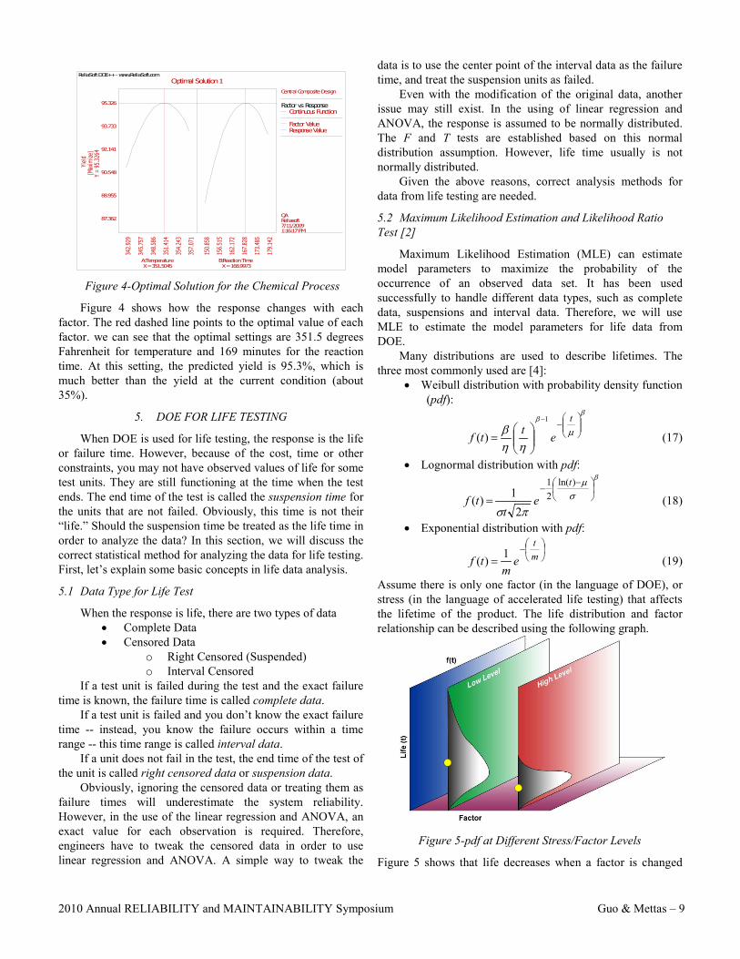
Figure 4-Optimal Solution for the Chemical Process
Figure 4 shows how the response changes with each factor. The red dashed line points to the optimal value of each factor. we can see that the optimal settings are 351.5 degrees Fahrenheit for temperature and 169 minutes for the reaction time. At this setting, the predicted yield is 95.3%, which is much better than the yield at the current condition (about 35%).
5. DOE FOR LIFE TESTING
When DOE is used for life testing, the response is the life or failure time. However, because of the cost, time or other constraints, you may not have observed values of life for some test units. They are still functioning at the time when the test ends. The end time of the test is called the suspension time for the units that are not failed. Obviously, this time is not their “life.” Should the suspension time be treated as the life time in order to analyze the data? In this section, we will discuss the correct statistical method for analyzing the data for life testing. First, let’s explain some basic concepts in life data analysis.
5.1 Data Type for Life Test
When the response is life, there are two types of data • Complete Data • Censored Data
o Right Censored (Suspended) o Interval Censored
If a test unit is failed during the test and the exact failure time is known, the failure time is called complete data.
If a test unit is failed and you don’t know the exact failure time -- instead, you know the failure occurs within a time range -- this time range is called interval data.
If a unit does not fail in the test, the end time of the test of the unit is called right censored data or suspension data.
Obviously, ignoring the censored data or treating them as failure times will underestimate the system reliability. However, in the use of the linear regression and ANOVA, an exact value for each observation is required. Therefore, engineers have to tweak the censored data in order to use linear regression and ANOVA. A simple way to tweak the
data is to use the center point of the interval data as the failure time, and treat the suspension units as failed.
Even with the modification of the original data, another issue may still exist. In the using of linear regression and ANOVA, the response is assumed to be normally distributed. The F and T tests are established based on this normal distribution assumption. However, life time usually is not normally distributed.
Given the above reasons, correct analysis methods for data from life testing are needed.
5.2 Maximum Likelihood Estimation and Likelihood Ratio Test [2]
Maximum Likelihood Estimation (MLE) can estimate model parameters to maximize the probability of the occurrence of an observed data set. It has been used successfully to handle different data types, such as complete data, suspensions and interval data. Therefore, we will use MLE to estimate the model parameters for life data from DOE.
Many distributions are used to describe lifetimes. The three most commonly used are [4]:
• Weibull distribution with probability density function (pdf):
ββ
µηη
β
−
−
=
t
ettf1
)( (17)
• Lognormal distribution with pdf: β
σµ
πσ
−
−=
)ln(21
21)(
t
et
tf (18)
• Exponential distribution with pdf:
−
= mt
em
tf 1)( (19)
Assume there is only one factor (in the language of DOE), or stress (in the language of accelerated life testing) that affects the lifetime of the product. The life distribution and factor relationship can be described using the following graph.
Figure 5-pdf at Different Stress/Factor Levels
Figure 5 shows that life decreases when a factor is changed
ReliaSoft DOE++ - www.ReliaSoft.comOptimal Solution 1
A:TemperatureX = 351.5045
B:Reaction TimeX = 168.9973
Y =
95.3
264
(Max
imize
)Yi
eld
342.
929
357.
071
345.
757
348.
586
351.
414
354.
243
87.362
95.326
88.955
90.548
92.141
93.733
150.
858
179.
142
156.
515
162.
172
167.
828
173.
485
Central Composite Design
Factor vs ResponseContinuous Function
Factor ValueResponse Value
QAReliasoft7/11/20091:16:17 PM

10 – Guo & Mettas 2010 AR&MS Tutorial Notes
from the low level to the high level. The pdf curves have the same shape while only the scale of the curve changes. The scale of the pdf is compressed at the high level. It means the failure mode remains the same, only the time of occurrence decreases at the high level. Instead of considering the entire scale of the pdf, a life characteristic can be chosen to represent the curve and used to investigate the effect of potential factors on life. The life characteristics for the three commonly used distributions are:
• Weibull distribution: η • Lognormal distribution: µ • Exponential distribution: m
The life-factor relationship is studied to see how factors affect life characteristic. For example, a linear model can be used as the initial investigation for the relationship:
......' 211221110 +++++= XXXX ββββµ (20) Where: )ln(' ηµ = for Weibull; µµ =' for lognormal and
)ln(' m=µ for exponential. Please note that in equation (20) a logarithmic
transformation is applied to the life characteristics of the Weibull and exponential distributions. One of the reasons is because η and m can take only positive values.
To test whether or not one effect in equation (20) is significant, the likelihood ratio test is used:
model) full()removedk effect (ln2)(effect
LLkLR −= (21)
Where L() is the likelihood value. LR follows a chi-squared distribution if effect k is not significant.
If effect k is not significant, whether or not it is removed from the full model of equation (20) will not affect the likelihood value much. It means the value of LR will be close to 0. Otherwise, if the LR value is very large, it means effect k is significant.
5.3 Life Test Example
Consider an experiment to improve the reliability of fluorescent lights [2]. Five factors A-E are investigated in the experiment. A 252 − design with factor generators D=AC and E=BC is conducted. The objective is to identify the significant effects that affect the reliability. Two replicates are used for each treatment. The test ends at the 20th day. Inspections are conducted every two days. The experiment results are given in Table 20.
Run A B C D E Failure Time
1 -1 -1 -1 -1 -1 (14,16) 20+
2 -1 -1 1 1 1 (18,20) 20+
3 -1 1 -1 -1 1 (8,10) (10, 12) 4 -1 1 1 1 -1 (18,20) 20+
5 1 -1 -1 1 -1 20+ 20+
6 1 -1 1 -1 1 (12,14) 20+
7 1 1 -1 1 1 (16,18) 20+
8 1 1 1 -1 -1 (12,14) (14, 16)
Table 20- Data for the Life Test Example
20+ means that the test unit was still working at the end of the test. So this experiment has suspension data. (14, 16) means that failure occurred at a time between the 14th and the 16th day. So this experiment also has interval data. The Weibull model is used as the distribution for the life of the fluorescent lights. The likelihood ratio test table is given below.
Model Effect DF Ln(LKV) LR P Value
Reduced A 1 -20.7181 3.1411 0.0763
B 1 -24.6436 10.9922 0.0009 C 1 -19.2794 0.2638 0.6076
D 1 -25.7594 13.2237 0.0003 E 1 -21.0727 3.8504 0.0497
Full 7 -19.1475
Table 21- LR Test Table for the Life Test Example
Table 21 has a layout that is similar to the ANOVA table. This makes it easy to read for engineers who are familiar with ANOVA. From the P value column, we can see factor A, B, D and E are important to the product life. The estimated factor-life relationship is:
EDCBA
1166.02477.00294.02256.01052.09959.2)ln(
+−−−+=η (22)
The estimated shape parameter β for the Weibull distribution is 7.27.
For comparison, the data was also analyzed using traditional linear regression and the ANOVA method. To apply linear regression and ANOVA, the data set was modified by using the center points as the failure time for interval data and treating the suspensions as failures. Results are given below.
Source of Variation DF Sum of
Squares Mean
Squares F Ratio P Value
Model 5 143.3125 28.6625 4.2384 0.025
A 1 1.5625 1.5625 0.2311 0.6411
B 1 33.0625 33.0625 4.8891 0.0515
C 1 3.0625 3.0625 0.4529 0.5162
D 1 95.0625 95.0625 14.0573 0.0038
E 1 10.5625 10.5625 1.5619 0.2398
Residual 10 67.625 6.7625
Total 15 210.9375
Table 23- ANOVA Table for the Life Test Example
In Table 23, only effects B and D are showing to be significant. The estimated linear regression model is:
EDCBAY
8127.04375.24375.04375.13125.09375.16
+−+−+= (23)
Comparing the results in Tables 22 and 23, we can see that they are quite different. The linear regression and ANOVA method failed to identify A and E as important

2010 Annual RELIABILITY and MAINTAINABILITY Symposium Guo & Mettas – 11
factors at the significance level of 0.1.
6. CONCLUSION
In this tutorial, simple examples were used to illustrate the basic concepts in DOE. Guidelines for conducting DOE were given. Three major topics were discussed in detail: 2-level factorial design, RSM and DOE for life tests.
Linear regression and ANOVA are the important tools in DOE data analysis. So, they are emphasized. For DOE involving censored data, the better method of MLE and likelihood ratio test should be used.
DOE involves many different statistical methods. Many useful techniques, such as blocking and randomization, random and mixed effect model, model diagnostic, power and sample size, measurement system study, RSM with multiple responses, D-optimal designs, Taguchi orthogonal array, Taguchi robust designs, mixture designs and so on are not covered in this tutorial [1, 2, 5, 6]. However, with the basic
knowledge of this tutorial, readers should be able to learn most of them easily.
REFERENCES
1. D. C. Montgomery, Design and Analysis of Experiments, 5th edition, John Wiley and Sons, Inc. New York, 2001.
2. C. F. Wu and M. Hamad, Experiments: Planning, Analysis, and Parameter Design Optimization, John Wiley and Sons, Inc. New York, 2000.
3. ReliaSoft, http://www.ReliaSoft.com/doe/index.htm 4. ReliaSoft, Life Data Analysis Reference, ReliaSoft
Corporation, Tucson, 2007. 5. R. H. Myers and D. C. Montgomery, Response Surface
Methodology: Process and Product Optimization Using Designed Experiments, 2nd edition, John Wiley and Sons, Inc. New York, 2002.
6. ReliaSoft, Experiment Design and Analysis Reference, ReliaSoft Corporation, Tucson, 2008.

12 – Guo & Mettas 2010 AR&MS Tutorial Notes
2010 RAMS –Tutorial DOE – Guo and Mettas 1
Design of Experiments (DOE) and Data Analysis
Huairui (Harry) Guo, Ph.D.Adamantios Mettas
San Jose, CA USA
January 25-28, 2010
2010 RAMS –Tutorial DOE – Guo and Mettas 3
Introduction
Introduction
Statistical Background
Two LevelFactorial Design
Response Surface Method
Reliability DOE
Summary
Tutorial: Design of Experiments (DOE) and Data Analysis
2010 RAMS –Tutorial DOE – Guo and Mettas 5
What DOE Can Do
Comparisons Variable screening Transfer function exploration System optimization System robustness
2010 RAMS –Tutorial DOE – Guo and Mettas 2
Outline Introduction
Why DOE What DOE Can Do Common Design Types General Guidelines for Conducting DOE
Statistic Background Linear Regression and Analysis of Variance (ANOVA)
Two Level Factorial Design Response Surface Method Reliability DOE
2010 RAMS –Tutorial DOE – Guo and Mettas 4
Why DOE
DOE Makes Your Life Easier Example 1
Usage voltage: V=10v Test all the 50 units at V=25v to predict the reliability at V=10v
Example 2 Usage temperature T=40 (Celsius) and humidity H=50% Accelerated life testing to predict reliability at usage level
Temperature(Celsius)
25 120 9525 85 85
Num of Units Humidity (%)
2010 RAMS –Tutorial DOE – Guo and Mettas 6
Common Design Types For comparison One factor design
For variable screening 2 level factorial design Plackett-Burman design Taguchi orthogonal array design
For transfer function identification and optimization Central composite design Box-Behnken design
For system robustness Taguchi robust design

2010 Annual RELIABILITY and MAINTAINABILITY Symposium Guo & Mettas – 13
2010 RAMS –Tutorial DOE – Guo and Mettas 7
General Guidelines for Conducting DOE
Clarify and state objective Choose responses Choose factors and levels Choose experimental design Perform the experiment Analyze the data Draw conclusions and make recommendations
2010 RAMS –Tutorial DOE – Guo and Mettas 9
Statistical Background Linear regression It is the foundation for DOE data analysis.
ANOVA (analysis of variance) ANOVA is a way to present the findings from the
linear regression model. ANOVA can tell you if there is a strong relationship
between the independent variables, Xs, and the response variable, Y.
ANOVA can test whether or not an individual X can affect Y significantly.
2010 RAMS –Tutorial DOE – Guo and Mettas 11
It is assumed to be normally distributed with mean of 0 and variance of
Linear Regression (cont’d)
Model
2σ
εβββ ++++= pp XXY ...110 Assumptions
:ε The random error or noise.
:Y For a given model, the response is also normally distributed and
),0(~ σε N
2)( σ=YVar
Parameter Estimation: Least Squares Estimation
2010 RAMS –Tutorial DOE – Guo and Mettas 8
Statistical Background
Introduction
Statistical Background
Two LevelFactorial Design
Response Surface Method
Reliability DOE
Summary
Tutorial: Design of Experiments (DOE) and Data Analysis
2010 RAMS –Tutorial DOE – Guo and Mettas 10
Linear Regression
-1.0
-0.5
0.0
0.5
1.0
1.5
1880 1900 1920 1940 1960 1980 2000
Tem
pera
ture
Ano
mol
y (o F)
Year
Regression analysis is a statistical technique that attempts to explore and model the relationship between two or more variables.
A linear regression model attempts to explain the relationship between two or more variables using a straight line.
14 – Guo & Mettas 2010 AR&MS Tutorial Notes
2010 RAMS –Tutorial DOE – Guo and Mettas 12
Example: Linear Regression
εβββ +++= 22110 XXY Within-run Variations For the same values of X1
and X2, the observed Y values are different.
This difference of Y is caused by noise.
Between-run Variations For different values of X1
and X2, the observed mean values of Y are different.
This difference of Y is caused by the different values of the Xs.
2010 RAMS –Tutorial DOE – Guo and Mettas 13
Measure the Variation Sum of Squares:
Mean Squares:
( )∑=
−=n
iiT YYSS
1
2
( )∑=
−−
=−
=n
ii
TT YY
nnSS
MS1
2
11
1
Mean Squares is the normalized variation of a data set. It is also the unbiased estimation of the variance of Y.
n: Number of observations. (It is 6 for this example.)
2010 RAMS –Tutorial DOE – Guo and Mettas 15
Partition the Sum of Squares of Regression The SSR can be divided into the variation caused by each
variable:
pXXXR SSSSSSSS +++= ...21
Each X has its own mean squares
PXXX MSMSMS ,..., ,21
The mean squares of each source is compared with MSE
If MSXi is significantly larger than MSE, Xi significantly affects Y. If it is not significantly larger than MSE, Xi’s effect is close to the
effect of noise. Xi doesn’t significantly affect Y.
2010 RAMS –Tutorial DOE – Guo and Mettas 17
ANOVA Table for the Example
Source of Variation
Degrees of Freedom
Sum of Squares
Mean Squares F Ratio
P Value
Model 2 6.14E+04 3.07E+04 36.86 0.0077 X1 1 6.00E+04 6.00E+04 72.03 0.0034 X2 1 8100 8100 9.72 0.0526
Residual 3 2500 833.3333Total 5 6.39E+04
P Value: The smaller the P value is, the more significant the corresponding source.The P value is compared with a given significance level, alpha. If a P value is less than the alpha, the corresponding source is significant at the significance level of alpha. The commonly used alpha values are 0.01, 0.05, 0.1.
The Model and X1 are significant at Level of 0.05.The Model, X1 and X2 are significant at Level of 0.1.
* Residual is the estimated value for error or noise.
2010 RAMS –Tutorial DOE – Guo and Mettas 14
Partition the Total Variation The total variation of Y includes two parts
Between-run Variation Within-run Variation ∑∑
==−+−=
+=n
iii
n
ii
ERT
YYYY
SSSSSS
1
2
1
2 )ˆ()ˆ(
SSR: Sum of Squares of Regression. The amount of variation explained by Xs.
SSE: Sum of Squares of Error. The amount of variation caused by noise.
pSSMS R
R = pnSSMS E
E −−=
1n: Number of observations p: Number of Xs. It is 2 for the previous example.
Mean squares of regression and error
2010 RAMS –Tutorial DOE – Guo and Mettas 16
Analysis of Variance (ANOVA)
F test for the regression model:
F test for each variable xi:
E
RMSMSF =0
H0: There is no difference between the variation caused by Xs and the variation caused by noise.
H1: The variation caused by Xs is larger than the variationcaused by noise.
E
X
MSMS
F i=0
H0: There is no difference between the variation caused by Xi and the variation caused by noise.
H1: The variation caused by Xi is larger than the variationcaused by noise.
2010 Annual RELIABILITY and MAINTAINABILITY Symposium Guo & Mettas – 15
2010 RAMS –Tutorial DOE – Guo and Mettas 18
T-test is an alternative to the F-test. T-test is used to test whether or not a coefficient is 0.
For example, H0: β1 = 0; H1: β1 ≠ 0
The test statistic is:
T-test for the Coefficients
)ˆ(
ˆ
1
10
ββ
seT =
1β is the estimated value for β1. )ˆ( 1βse is the standard error.
Under the Null-hypothesis, T0 follows the t distribution with the degree of freedom (df) that is the same as the df of the error term.
2010 RAMS –Tutorial DOE – Guo and Mettas 19
T-test Results
Term CoefficientStandard
Error T Value P ValueIntercept -2135 588.7624 -3.6263 0.0361
X 1 7 0.8248 8.487 0.0034X 2 18 5.7735 3.1177 0.0526
Note: The P values from the T-test are the same as in the F-test.
Source of Variation
Degrees of Freedom
Sum of Squares
Mean Squares F Ratio
P Value
Model 2 6.14E+04 3.07E+04 36.86 0.0077 X1 1 6.00E+04 6.00E+04 72.03 0.0034 X2 1 8100 8100 9.72 0.0526
Residual 3 2500 833.3333Total 5 6.39E+04
2010 RAMS –Tutorial DOE – Guo and Mettas 21
Two Level Factorial Design
Introduction
Statistical Background
Two LevelFactorial Design
Response Surface Method
Reliability DOE
Summary
Tutorial: Design of Experiments (DOE) and Data Analysis
2010 RAMS –Tutorial DOE – Guo and Mettas 23
Some Basic Concepts in DOE Treatment: A unique combination of all the factors. Replicate: The number of test units under each
treatment.
Treatment = 4 Replicate = 1
k2 k is the number of factors. Design notation:
2010 RAMS –Tutorial DOE – Guo and Mettas 20
Pareto Chart for the T-ValuesReliaSoft DOE++ - www.ReliaSoft.com
Pareto Chart
Alpha = 0.1; Threshold = 2.3534Effect
Term
0.000 9.0003.600 5.400 7.2002.353
X2
X1
Pareto Chart
Critical ValuSignificant
QAReliasoft7/28/20094:57:54 PM

16 – Guo & Mettas 2010 AR&MS Tutorial Notes
2010 RAMS –Tutorial DOE – Guo and Mettas 22
Two Level Factorial Design Why two levels? To study the effect of a factor or a variable, at least two
different settings are needed. High = 1, Low = -1. From a linear regression viewpoint, you need at least
two points to fit a straight line.
Example 1 Usage voltage: V=10v Test all the 50 units at V=25v to predict the reliability at V=10v.
Answer to the first example
2010 RAMS –Tutorial DOE – Guo and Mettas 24
Balanced and Orthogonal
Orthogonal: The sum of the product of each factor column is 0.
0)11()11()11()11( =×+×−+−×+−×−
Balanced: The number of test units is the same for all the treatments.
A balanced and orthogonal design can evaluate the effect of each factor more accurately.
If you add one more sample for any one of the treatments, the design will be unbalanced and non-orthogonal.
2010 RAMS –Tutorial DOE – Guo and Mettas 25
Linear Model for 2 Factorial Design
Main effect: effect A(X1) and B(X2)
Two-way interaction effect: AB(X1X2) The number of factors in a interaction effect is the
order of the interaction. ANOVA is used to test whether or not an effect is
significant.
εββββ ++++= 211222110 XXXXY
X1: Factor A, X2: Factor B
2010 RAMS –Tutorial DOE – Guo and Mettas 27
Two Level Fractional Factorial Design
Why fractional factorial design Reduce the sample size. For a 7 factor design, you need
27 = 128 runs. Reduce cost and time by only using part of the full
design. Why fractional factorial design works Sparsity of effects principle: Most of the time,
responses are affected by only a small number of main effects and lower order interactions.
Fractional factorial design: Focus on main effects and lower order interactions.
2010 RAMS –Tutorial DOE – Guo and Mettas 29
Half Fractional Factorial Design 23-1
Order A B AB C AC BC ABC2 1 -1 -1 -1 -1 1 13 -1 1 -1 -1 1 -1 15 -1 -1 1 1 -1 -1 18 1 1 1 1 1 1 1
From this experiment, the effect of AB and C, AC and B, and BC and A cannot be distinguished. Each pair of columns (AB and C, A and BC, B and AC) have the same pattern.
Effects that cannot be distinguished within a design are called Confounded Effects or Aliased Effects.
The summary of the aliased effects for the design is called Alias Structure.
I=ABC is called the Defining Relation.
[I]=I+ABC; [A]=A+AC; [B]=B+BC; [C]=C+AB
2010 RAMS –Tutorial DOE – Guo and Mettas 26
A Simple Way to Estimate the Coefficients Least Square Estimation is used for any design
102
25202
3530
Aat Avg. - Aat Avg. A ofEffet lowhigh
=+
−+
=
=
12 A ofEffect β=
Special case: only valid for a balanced design

2010 Annual RELIABILITY and MAINTAINABILITY Symposium Guo & Mettas – 17
2010 RAMS –Tutorial DOE – Guo and Mettas 28
Design Matrix for a 23 Design
If effect ABC can be ignored in the study, then we can select the treatments with ABC=1 for a Fractional Factorial Design.
2010 RAMS –Tutorial DOE – Guo and Mettas 30
Generate a Fractional Factorial Design
Order A B C AB AC BC ABC2 1 -1 -1 -1 -1 1 13 -1 1 -1 -1 1 -1 15 -1 -1 1 1 -1 -1 18 1 1 1 1 1 1 1
The design is a Full Factorial Design for A and B. A and B are called Basic Factors. The Full Factorial Design for A and B is called the Basic
Design. Factor C can be generated from C = AB. C = AB is called the Factor Generator for C.
2010 RAMS –Tutorial DOE – Guo and Mettas 31
Review the Second Example
Example 2 Usage temperature T=40 (C) and humidity H=50%. Accelerated life test to predict reliability at usage level.
Temperature(Celsius)
25 120 (+1) 95 (+1)25 85 (-1) 85 (-1)
Num of Units Humidity (%)
It is a bad design: Main effects Temperature and Humidity are Confounded.
From the viewpoint of Linear Regression, at least 3 unique combinations are needed — why?
εβββ +++= 22110 XXY
2010 RAMS –Tutorial DOE – Guo and Mettas 33
Fractional Factorial Design Example (cont’d)
With five factors the total number of runs required for a full factorial is 25 = 32. These runs are too expensive for the manufacturer.
Only the main effects and the two factor interactions are assumed to be important.
It is decided to carry out the investigation using the 25-1
design (requiring 16 runs) with the factor generator E= ABCD.
2010 RAMS –Tutorial DOE – Guo and Mettas 35
ANOVA Table with All EffectsSource of Variation DF Sum of
SquaresMean
Squares F P Value
Model 15 5775.4375 385.0292 - -A 1 495.0625 495.0625 - -B 1 4590.0625 4590.0625 - -C 1 473.0625 473.0625 - -D 1 3.0625 3.0625 - -E 1 1.5625 1.5625 - -
AB 1 189.0625 189.0625 - -AC 1 0.5625 0.5625 - -AD 1 5.0625 5.0625 - -AE 1 5.0625 5.0625 - -BC 1 1.5625 1.5625 - -BD 1 0.0625 0.0625 - -BE 1 0.0625 0.0625 - -CD 1 3.0625 3.0625 - -CE 1 0.5625 0.5625 - -DE 1 7.5625 7.5625 - -
Residual 0Total 15 5775.4375

18 – Guo & Mettas 2010 AR&MS Tutorial Notes
2010 RAMS –Tutorial DOE – Guo and Mettas 32
Fractional Factorial Design Example The yield in the manufacture of
integrated circuits is thought to be affected by the following five factors*:
The objective of the experimentation is to increase the yield by finding the significant effects.
A Aperture Setting small largeB Exposure Time minutes 20 40C Develop Time seconds 30 45D Mask Dimension small largeE Etch Time minutes 14.5 15.5
Factor Name Unit Low High
* Montgomery, D. C, 2001
2010 RAMS –Tutorial DOE – Guo and Mettas 34
Run Order A B C D E Yield1 1 -1 -1 1 1 102 1 -1 1 1 -1 213 -1 1 1 -1 1 454 -1 -1 1 -1 -1 165 1 1 -1 -1 1 526 1 1 1 -1 -1 607 -1 1 -1 1 1 308 -1 -1 1 1 1 159 1 -1 -1 -1 -1 9
10 -1 1 -1 -1 -1 3411 -1 -1 -1 -1 1 812 1 1 -1 1 -1 5013 -1 1 1 1 -1 4414 -1 -1 -1 1 -1 615 1 -1 1 -1 1 2216 1 1 1 1 1 63
Design Matrix and Observations
Run Order: The test sequence of the treatments. The experiment is conducted in a Random Sequence of the factor combinations.
2010 RAMS –Tutorial DOE – Guo and Mettas 36
Identify Significant EffectsReliaSoft DOE++ - www.ReliaSoft.com
Normal Probability Plot of Effect
Alpha = 0.1; Lenth's PSE = 0.9375
Effect
Prob
ability
-40.000 40.000-24.000 -8.000 8.000 24.0001.000
5.000
10.000
50.000
99.000
AB
C:Develop Time
A:Aperture Setting
B:Exposure Time
Effect Probability
YieldY' = Y
Non-Significant EffectsSignificant EffectsDistribution Line
QAReliasoft7/10/20093:03:18 PM
Lenth’s method assumes all the effects should be normally distributed with a mean of 0, given the hypothesis that they are not significant.
2010 RAMS –Tutorial DOE – Guo and Mettas 37
Pool Non-Significant Effects to Error
Non-significant effects are treated as “noise” and are used to estimate the error.
2010 RAMS –Tutorial DOE – Guo and Mettas 39
Response Surface Methods (RSM)
RSM is used to estimate the transfer function at the optimal region.
The Quadratic model is used in RSM. The estimated function is used for optimization. Linear regression and ANOVA are the tools for
data analysis.
2010 RAMS –Tutorial DOE – Guo and Mettas 41
Design Matrix for the Initial Investigation Experiment
The initial design at the current operation condition is used to search the direction for locating the optimal region for optimization.
The initial design is a modified factorial design. The Design Matrix is:A: B:
Temperature Reaction Time 1 1 -1 -1 33.952 1 1 -1 36.353 1 -1 1 354 1 1 1 37.255 0 0 0 35.456 0 0 0 35.757 0 0 0 36.058 0 0 0 35.39 0 0 0 35.9
Std. Order Point Type Yield (%)

2010 Annual RELIABILITY and MAINTAINABILITY Symposium Guo & Mettas – 19
2010 RAMS –Tutorial DOE – Guo and Mettas 38
Response Surface Method
Introduction
Statistical Background
Two LevelFactorial Design
Response Surface Method
Reliability DOE
Summary
Tutorial: Design of Experiments (DOE) and Data Analysis
2010 RAMS –Tutorial DOE – Guo and Mettas 40
RSM: Example The yield from a chemical process has been
found to be affected by two factors: Reaction Temperature Reaction Time
The current operating conditions of 230 Fahrenheit and 65 minutes give a yield of about 35%.
The engineer decides to explore the current conditions in the range (225, 235)Fahrenheit and (55, 75) minutes so that steps can be taken to achieve the maximum yield.
2010 RAMS –Tutorial DOE – Guo and Mettas 42
Coded Values and Center Points
Coded value (-1, 0, 1)
Low andHigh Between Range theof HalfLow andHigh of Value Middle-Value Actual valueCoded =
For example, the temperature is (Low = 225, High = 235). So when Temperature = 230, the corresponding coded value is 0.
Reasons for using Center Points Replicates at Center Points can be used to estimate the random error. Replicates at Center Points will keep the Orthogonality of the design. Can be used to check whether or not the Linear Model is sufficient or
whether the curvature is significant.
2010 RAMS –Tutorial DOE – Guo and Mettas 43
Results for the Initial Experiment
* Curvature and AB are not significant.
ANOVA Table
The final linear regression model (in coded values) with only significant terms:
21 4875.01625.16375.35 XXY ++=
2010 RAMS –Tutorial DOE – Guo and Mettas 45
Path of Steepest Ascent
A B A BCurrent
Operation 0 0 230 65 35
1 2.4 1 242 75 36.52 4.8 2 254 85 39.353 7.2 3 266 95 45.654 9.6 4 278 105 49.555 12 5 290 115 55.76 14.4 6 302 125 64.257 16.8 7 314 135 72.58 19.2 8 326 145 80.69 21.6 9 338 155 91.4
10 24 10 350 165 95.4511 26.4 11 362 175 89.312 28.8 12 374 185 87.65
Yield (%)Coded ActualStepFactor Levels

20 – Guo & Mettas 2010 AR&MS Tutorial Notes
2010 RAMS –Tutorial DOE – Guo and Mettas 47
Factorial Design Around the Optimal RegionStd. Order Point Type A:Temperature (F) B:Reaction Time (min) Yield (%)
1 1 345 155 89.752 1 355 155 90.23 1 345 175 924 1 355 175 94.255 0 350 165 94.856 0 350 165 95.457 0 350 165 958 0 350 165 94.559 0 350 165 94.7
At the optimal region, the curvature is significant. The simple linear model is not enough any more.
2010 RAMS –Tutorial DOE – Guo and Mettas 44
Direction of Steepest Ascent21 4875.01625.16375.35 XXY ++=
The coefficients show that the direction is (1.1626, 0.4875) or can be normalized to (2.4, 1).
The direction of steepest ascent is perpendicular to the contour lines.
2010 RAMS –Tutorial DOE – Guo and Mettas 46
Further Investigation at the Optimal Region
From the sequential tests, we found the setting at step 10 (Temp = 350, Time = 165) is close to the optimal region.
The region around the setting at step 10 (Temp = 350, Time = 165) should be investigated.
A Factorial Design with a center point of (350, 165) was conducted.
2010 RAMS –Tutorial DOE – Guo and Mettas 48
Designs for Quadratic Model
Quadratic modelεββββββ ++++++= 2112
2222
211122110 XXXXXXY
Special designs are used for the Quadratic model. Central Composite Design (CCD) is one of them. CCD can be directly augmented from a regular
factorial design.
2010 RAMS –Tutorial DOE – Guo and Mettas 49
Augment a Factorial Design to a Central Composite Design
(1,1)
(1,-1)(-1,-1)
(-1,1)
(0, 0)(-α, 0)
(0, α)
(0, -α)
(α, 0)
(1,1)
(1,-1)(-1,-1)
(-1,1)
(0, 0)(-α, 0)
(0, α)
(0, -α)
(α, 0)
Using a 2 factor factorial design as example:
The points outside the rectangle are called axial points or star points.
2010 RAMS –Tutorial DOE – Guo and Mettas 51
The Complete CCD Matrix for the ExampleStd. Order Point Type A:Temperature (F) B:Reaction Time (min) Yield (%)
1 1 345 155 89.752 1 355 155 90.23 1 345 175 924 1 355 175 94.255 0 350 165 94.856 0 350 165 95.457 0 350 165 958 0 350 165 94.559 0 350 165 94.7
10 -1 342.93 165 90.511 -1 357.07 165 92.7512 -1 350 150.86 88.413 -1 350 179.14 92.6
Four Star Points are added to the previous factorial design.

2010 Annual RELIABILITY and MAINTAINABILITY Symposium Guo & Mettas – 21
2010 RAMS –Tutorial DOE – Guo and Mettas 53
Model Diagnostic Check the residual plots
ReliaSoft DOE++ - www.ReliaSoft.comNormal Probability Plot of Residual
Anderson-Darling = 0.3202; p-value = 0.4906Residual
Proba
bility
-2.000 2.000-1.200 -0.400 0.400 1.2001.000
5.000
10.000
50.000
99.000 Residual Probability
YieldY' = Y
Data PointsResidual Line
QAReliasoft7/11/20091:07:07 PM
2010 RAMS –Tutorial DOE – Guo and Mettas 50
How to Decide α Several methods have been developed for deciding
α. Special values of α can make the design have special
properties, such as a design that can better estimate model parameters, or that can better explore the optimal region.
A commonly used method is:4/1
)(2
=
−
s
ffk
nn
α
nf is the number of replicates of the runs in the original factorial design.ns is the number of replicates of the runs at the axial points. 2k-f represents the original factorial or fractional factorial design.
2010 RAMS –Tutorial DOE – Guo and Mettas 52
Results from the Experiment
2122
2121 45.008.252.153.174.091.94 XXXXXXY +−−++=
ANOVA Table
Model in terms of coded value:
2010 RAMS –Tutorial DOE – Guo and Mettas 54
Model Diagnostic (cont’d)ReliaSoft DOE++ - www.ReliaSoft.com
Residual vs Run Order
Alpha = 0.1; Upper Critical Value = 0.6209; Lower Critical Value = -0.6209Run Order
Resid
ual
0.000 15.0003.000 6.000 9.000 12.000-0.700
0.700
-0.420
-0.140
0.140
0.420
0.621
-0.621
0.000
Residual vs Order
YieldY' = Y
Data PointsUpper Critical ValueLower Critical Value
Zero Value Line
QAReliasoft7/11/20091:08:33 PM
2010 RAMS –Tutorial DOE – Guo and Mettas 55
Optimization21
22
2121 45.008.252.153.174.091.94 XXXXXXY +−−++=
ReliaSoft DOE++ - www.ReliaSoft.comOptimal Solution 1
A:TemperatureX = 351.5045
B:Reaction TimeX = 168.9973
Y =
95.3
264
(Max
imize
)Yi
eld
342.
929
357.
071
345.
757
348.
586
351.
414
354.
243
87.362
95.326
88.955
90.548
92.141
93.733
150.
858
179.
142
156.
515
162.
172
167.
828
173.
485
Central Composite Design
Factor vs ResponseContinuous Function
Factor ValueResponse Value
QAReliasoft7/11/20091:16:17 PM
Optimal Setting (Temperature = 351.5, Time = 169.0) Predicted Yield at the Optimal Setting is 95.3%

22 – Guo & Mettas 2010 AR&MS Tutorial Notes
2010 RAMS –Tutorial DOE – Guo and Mettas 57
DOE For Life Testing The response is the failure time.
The failure time usually is not normally distributed, so linear regression and ANOVA are not good for life data.
If a unit is still running at the time when the test ends, you only have suspension time, not failure time for this unit.
The correct analysis method is needed for reliability DOE. A method that can handle lifetime distributions such as Weibull,
lognormal and exponential. A method that can handle suspension times correctly. A method that can evaluate the significance of each effect,
similar to ANOVA.
2010 RAMS –Tutorial DOE – Guo and Mettas 59
Right Censored (Suspended) Data: Example
Imagine that we tested five units and three failed. In this scenario, our data set is composed of the times-to-failure of the three units that failed and the running time of the other two units that did not fail.
2010 RAMS –Tutorial DOE – Guo and Mettas 56
Reliability DOE (R-DOE)
Introduction
Statistical Background
Two LevelFactorial Design
Response Surface Method
Reliability DOE
Summary
Tutorial: Design of Experiments (DOE) and Data Analysis
2010 RAMS –Tutorial DOE – Guo and Mettas 58
Data Types
Complete data
Censored data Right Censored
Interval Censored
?
?
2010 RAMS –Tutorial DOE – Guo and Mettas 60
Interval Censored Data: Example
Imagine that we are running a test on five units and inspecting them every 100 hours. If a unit failed between inspections, we do not know exactly when it failed, but rather that it failed between inspections. This is also called “inspection data.”
2010 RAMS –Tutorial DOE – Guo and Mettas 61
Distributions Commonly Used in Reliability
Weibull distribution pdf:
Lognormal distribution pdf:
Exponential distribution pdf:
β
ηβ
ηηβ
−
−
=
t
ettf1
)(
21 ln( )21( )
2
t
f t et
µσ
σ π
− − =
−
= mt
em
tf 1)(

2010 Annual RELIABILITY and MAINTAINABILITY Symposium Guo & Mettas – 23
2010 RAMS –Tutorial DOE – Guo and Mettas 63
Life-Factor Relationship Simplify: Infer a Characteristic
Instead of considering the entire scale of the pdf, the life characteristic can be chosen to investigate the effect of potential factors on life.
The life characteristics for the three commonly used distributions are:
Weibull: Lognormal: Exponential:η µ m
2010 RAMS –Tutorial DOE – Guo and Mettas 65
The Likelihood Function Based on Life-Factor Relationship
Life-Factor Relationship
Failure Time Data
Suspension Data
Interval Data
MLE
...... 211222110' +++++= iiiii xxxx ββββµ
1
( ; , )N
f i ii
L f T µ σ=
′=∏
1
( ; , )M
S j ij
L R S µ σ=
′=∏
[ ]1
( ; , ) ( ; , )P
I Ul i Ll il
L F I F Iµ σ µ σ=
′ ′= −∏
0 1 2, , ,...β β β and σ for lognormal
IsfLLLL ××=
2010 RAMS –Tutorial DOE – Guo and Mettas 62
Combining Reliability and DOE: Life-Factor Relationship
The graphic shows an example where life decreases when a factor is changed from the low level to the high level.
It is seen that the pdf changes in scale only. The scale of the pdf is compressed at the high level.
The failure mode remains the same. Only the time of occurrence decreases at the high level.
2010 RAMS –Tutorial DOE – Guo and Mettas 64
Life-Factor Relationship Using the life characteristic, the model to investigate the effect of
factors on life can be expressed as:
Note that a logarithmic transformation is applied to the life characteristics of the Weibull and exponential distributions. This is because and m can take only positive values.
......' 211222110 +++++= xxxx ββββµ
where: )ln(' ηµ = or µµ =' or )ln(' m=µ
:jx jth factor value
η
2010 RAMS –Tutorial DOE – Guo and Mettas 66
Testing Effect Significance: Likelihood Ratio Test
( )( ) 2 ln( )
L effect k removedLR effect kL full Model
= −
21,( )LR effect k αχ>
Life-factor relationship:
Likelihood ratio test:
If then effect k is significant.
...... 211222110' +++++= iiiii xxxx ββββµ

24 – Guo & Mettas 2010 AR&MS Tutorial Notes
2010 RAMS –Tutorial DOE – Guo and Mettas 67
R-DOE: Example
Consider an experiment to improve the reliability of fluorescent lights. Five factors A-E are investigated in the experiment. A 25-2
design with factor generators D=AC and E=BC was conducted.*
Objective: To identify the significant factors and adjust them to improve life.
*Taguchi, 1987, p. 930.
2010 RAMS –Tutorial DOE – Guo and Mettas 69
Traditional DOE Approach
Assumes that the response (life) is normally distributed.
Treats suspensions as failures. Uses the middle point of the interval data as the
failure time. Problem: The above assumptions and adjustments
are incorrect.
2010 RAMS –Tutorial DOE – Guo and Mettas 71
MLE and Likelihood Ratio Test
Life-factor relation (Weibull distribution)
EDCBA
1166.02477.00294.02256.01052.09959.2)ln(
+−−−+=η
Likelihood Ratio (LR) Test Table
2010 RAMS –Tutorial DOE – Guo and Mettas 68
R-DOE: Example (cont’d)
Two replicates at each treatment. Inspections were conducted every two hours. Results have interval data and suspensions.
A B C D E-1 -1 -1 1 1 14~16 20+-1 -1 1 -1 -1 18~20 20+-1 1 -1 1 -1 8~10 10~12-1 1 1 -1 1 18~20 20+1 -1 -1 -1 1 20+ 20+1 -1 1 1 -1 12~14 20+1 1 -1 -1 -1 16~18 20+1 1 1 1 1 12~14 14~16
Failure Time
2010 RAMS –Tutorial DOE – Guo and Mettas 70
Fluorescent Lights R-DOE: Life-Factor Relationship
)1()1()1()1()1( 543210'1 +×++×+−×+−×+−×+= ββββββµ
For the ith observation
For example, for the first run, the equation is:
…assuming that the interactions are absent.
0 1 2 3 4 5' ...i i i i i iA B C D Eµ β β β β β β= + + + + + +A B C D E-1 -1 -1 1 1 14~16 20+-1 -1 1 -1 -1 18~20 20+-1 1 -1 1 -1 8~10 10~12-1 1 1 -1 1 18~20 20+1 -1 -1 -1 1 20+ 20+1 -1 1 1 -1 12~14 20+1 1 -1 -1 -1 16~18 20+1 1 1 1 1 12~14 14~16
Failure Time
2010 RAMS –Tutorial DOE – Guo and Mettas 72
Z-test for the Coefficients
Z-test is used to test whether or not a coefficient is 0. For example,
H0: β1 = 0; H1: β1 <> 0
The test statistic is:
)ˆ(
ˆ
1
10
ββ
seZ =
1β is the estimated value for β1. )ˆ( 1βse is the standard error.
Under the Null-hypothesis, Z0 is assumed to be standard normally distributed.

2010 Annual RELIABILITY and MAINTAINABILITY Symposium Guo & Mettas – 25
2010 RAMS –Tutorial DOE – Guo and Mettas 73
Z-test Results
When the sample size is large, they are very close. When the sample size is small, the likelihood ratio test is more
accurate than the Z-test.
Note: The P values from the Z-test are slightly different from the Likelihood Ratio test.
2010 RAMS –Tutorial DOE – Guo and Mettas 75
Model Diagnostic When using the Weibull distribution for life, the residuals from the life-
factor relationship should follow the extreme value distribution with a mean of zero.
2010 RAMS –Tutorial DOE – Guo and Mettas 77
Fluorescent Lights R-DOE: Interpreting the Results From the results, factors A,B, D and E are significant at the risk level of
0.10. Therefore, attention should be paid to these factors.
In order to improve the life, factors A and E should be set to the high level; while factors B and D should be set to the low level.
Term CoefficientA:A 0.1052B:B -0.2256C:C -0.0294D:D -0.2477E:E 0.1166
MLE Information
2010 RAMS –Tutorial DOE – Guo and Mettas 74
Pareto Chart for the Z-values
ReliaSoft DOE++ - www.ReliaSoft.comPareto Chart
Standardized Effect (Z Value)
Term
0.000 5.0001.000 2.000 3.000 4.0001.645
C:C
A:A
E:E
B:B
D:D
Pareto Chart
Critical ValueNon-SignificantSignificant
QAReliasoft7/11/20099:06:30 PM
From both LR test and the Z-test, A, B, D and E are significant.
Z-values are the normalized coefficients.
2010 RAMS –Tutorial DOE – Guo and Mettas 76
Model Diagnostic (cont’d)Residuals against run order plot
2010 RAMS –Tutorial DOE – Guo and Mettas 78
Fluorescent Lights Example: Traditional DOE Approach Suspensions are treated as failures. Mid-points are used as failure times for interval data. Life is assumed to follow the normal distribution.

26 – Guo & Mettas 2010 AR&MS Tutorial Notes
2010 RAMS –Tutorial DOE – Guo and Mettas 79
Traditional DOE Approach: Fluorescent Lights Example - Results
B and D come out to be significant using traditional DOE approach. A, B, D and E were found to be significant using R-DOE. Traditional DOE fails to identify A and E as important factors at a
significance level of 0.1.
2010 RAMS –Tutorial DOE – Guo and Mettas 81
Summary: Topics Covered
Why DOE, what DOE can do and common design types
General guidelines for conducting DOE Linear regression and ANOVA 2-level factorial and fractional factorial design Response surface method Reliability DOE
2010 RAMS –Tutorial DOE – Guo and Mettas 83
More Information On-line textbook and examples http://www.weibull.com/doewebcontents.htm http://www.itl.nist.gov/div898/handbook/
2010 RAMS –Tutorial DOE – Guo and Mettas 80
Summary
Introduction
Statistical Background
Two LevelFactorial Design
Response Surface Method
Reliability DOE
Summary
Tutorial: Design of Experiments (DOE) and Data Analysis
2010 RAMS –Tutorial DOE – Guo and Mettas 82
Topics Not Covered
Blocking Power and sample size RSM with multiple responses RSM: Box-Behnken design D-optimal design Taguchi robust design Taguchi orthogonal array (OA) Mixture design Random and mixed effect model …more

2010 Annual RELIABILITY and MAINTAINABILITY Symposium Guo & Mettas – 27
2010 RAMS –Tutorial DOE – Guo and Mettas 84
The End