© 2002

by

Joseph Richard Spadea

Title

Approved by Supervising Committee:

Supervisor Name (no title), Supervisor

2nd Reader Name (no title), Supervisor

Dedication

Your words here.

Acknowledgements

Your acknowledgements here.

Date

iv

Abstract

Title

Your Official UT Name, Previous Degree

The University of Texas at Austin, 2000

Supervisors: Supervisor Name and Second Reader Name

Abstract text here.

v

Table of Contents

vi

List of Tables

vii

viii

List of Figures

Fatigue Strength of Fillet-Welded Transverse Stiffeners

With Undercuts

by

Joseph Richard Spadea, B.S.C.E.

Thesis

Presented to the Faculty of the Graduate School of

The University of Texas at Austin

in Partial Fulfillment

of the Requirements

for the Degree of

Master of Science in Engineering

The University of Texas at Austin

May 2002

Fatigue Strength of Fillet-Welded Transverse Stiffeners

With Undercuts

Approved by Supervising Committee:

Karl H. Frank

Michael D. Engelhardt

Dedication

To my parents and grandparents Salvato, John and Mike for their encouragement

and love throughout my academic studies.

To my late grandparents Vincent and Barbara Spadea, for their fortitude and

perseverance in realizing the American Dream.

Acknowledgements

This thesis is based on research sponsored by the Texas Department of

Transportation for the Center for Transportation Research at the Phil M. Ferguson

Structural Engineering Laboratory at the University of Texas at Austin.

I would like to express my sincerest thanks to my advisor Dr. Karl H.

Frank, for it was an honor and privilege learning from him. I am very grateful for

his guidance, advice, and friendship throughout the research project. I would also

like to thank Dr. Michael D. Engelhardt for his time and suggestions in reviewing

this thesis.

To Blake Stasney, Mike Bell, Dennis Fillip and Ray Madonna for their

technical expertise and assistance in the laboratory. Thank you for your efforts

and time when I needed it most. The results of this thesis would not be possible

without their insight and willingness to lend a helping hand.

Lastly, I would like to thank my colleagues, the fine students of the

structural engineering department. You truly are the backbone of our prestigious

program and your friendship will be valued throughout my lifetime.

May 2002

v

Abstract

Fatigue Strength of Fillet-Welded Transverse Stiffeners

With Undercuts

Joseph Richard Spadea, M.S.E.

The University of Texas at Austin, 2002

Supervisor: Karl H. Frank, Michael D. Engelhardt

Steel girders are subjected to cyclic loading caused by the impact of

vehicular traffic on a daily basis. Poorly detailed stiffener attachments will result

in fatigue cracking of the girder. The effect of wrapping the stiffener-to-flange

weld upon the fatigue life was evaluated. The impact of undercuts at the stiffener

clip and flange edge upon fatigue strength was also determined. Several test

specimens were developed including a stiffener detail with no clip opening. It

was found that wrapping the welds around the stiffener had no impact upon the

fatigue life of the specimens.

vi

Table of Contents

CHAPTER 1 INTRODUCTION ............................................................................... 1

1.1 Introduction ............................................................................................. 1

1.2 Fabrication Survey .................................................................................. 5

1.3 Literature Survey ..................................................................................... 8

1.4 Scope of Work ....................................................................................... 21

CHAPTER 2 SPECIMEN DESIGN AND FABRICATION ....................................... 22

2.1 Introduction ........................................................................................... 22

2.2 Specimen Design ................................................................................... 27 2.2.1 Finite Element Model ................................................................ 33

2.3 Specimen Fabrication ............................................................................ 37 2.3.1 Materials and Welding Parameters ........................................... 37 2.3.2 Assembly ................................................................................... 38

2.4 Details of Weld Undercuts .................................................................... 42

2.5 Measuring of Undercuts ........................................................................ 47 2.5.1 Type A Specimen Undercuts ..................................................... 47 2.5.2 Type B Specimen Undercuts ..................................................... 49 2.5.3 Type C Specimen Undercuts ..................................................... 52 2.5.4 Type D Specimen Undercuts .................................................... 55

vii

CHAPTER 3 TEST SETUP ................................................................................... 58

3.1 Introduction ........................................................................................... 58

3.2 Test Apparatus ....................................................................................... 59 3.2.1 Test Frame Components ............................................................ 60 3.2.2 Hydraulic Supply ....................................................................... 61

3.3 Test Method ........................................................................................... 63 3.3.1 Parameters ................................................................................. 63 3.3.2 Test Procedure ........................................................................... 65

CHAPTER 4 FATIGUE TEST RESULTS .............................................................. 72

4.1 Introduction ........................................................................................... 72

4.2 Specimen Results .................................................................................. 75 4.2.1 Recording of Fatigue Cracks ..................................................... 76 4.2.2 Fracture Surfaces ....................................................................... 78

4.3 Data Analysis ........................................................................................ 90 4.3.1 Comparison with AASHTO Fatigue Resistance ....................... 90 4.3.2 Analysis of Variance ................................................................. 92

CHAPTER 5 SUMMARY AND CONCLUSIONS .................................................... 97

5.1 Evaluation of Test Results ..................................................................... 97

5.2 Recommendations ................................................................................. 98

BIBLIOGRAPHY……………………………………………………………..100

VITA……………………………………………………………………………10

3

viii

List of Tables

Table 1-1: Undercut Measurements (Janosch and Debiez, 1998) ........................ 13 Table 2-1: Specimen A Stiffener Undercut Measurements (inches) .................... 48 Table 2-2: Specimen B Stiffener Undercut Measurements (inches) .................... 50 Table 2-3: Specimen B Flange Undercut Measurements (inches) ....................... 51 Table 2-4: Specimen C Stiffener Undercut Measurements (inches) .................... 53 Table 2-5: Specimen C Flange Undercut Measurements (inches) ....................... 53 Table 2-6: Specimen C Flange Grinding Surface Measurements (inches) .......... 54 Table 2-7: Specimen D Stiffener Undercut Measurements (inches) .................... 56 Table 2-8: Average Undercut Dimensions ........................................................... 57 Table 3-1: 25 ksi Upper Stress Limit Readings ................................................... 68 Table 3-2: 5 ksi Lower Stress Limit Readings ..................................................... 68 Table 3-3: Average Upper & Lower Limit Stress Readings ................................ 68 Table 4-1: Summary of Fatigue Testing Results .................................................. 75 Table 4-2: Specimen Failure Locations ............................................................... 77 Table 4-3: Comparison of Actual and Predicted Fatigue Life ............................. 92 Table 4-4: Average Fatigue Life and Standard Deviation by Specimen Type .... 94 Table 4-5: Analysis of Variance Results .............................................................. 95 Table 5-1: Stiffener Undercut Summary (inches) ................................................ 98 Table 5-2: Flange Undercut Summary (inches) ................................................... 99

ix

List of Figures

Figure 1-1: Girder Diaphragm (TxDOT) ............................................................... 1 Figure 1-2: Stiffener-to-Flange Connections ......................................................... 2 Figure 1-3: Current Stiffener Weld Detail (TxDOT) ............................................. 3 Figure 1-4: Fully Wrapped Stiffener, No Clip ....................................................... 5 Figure 1-5: Girder in Fabrication Yard .................................................................. 6 Figure 1-6: Fully Wrapped Diaphragm Stiffener ................................................... 6 Figure 1-7: Wrapped Intermediate Stiffener Welds ............................................... 6 Figure 1-8: Specimen and Setup (Ruge and Woesle, 1962) .................................. 8 Figure 1-9: Types of Undercuts (Petershagen, 1990) ............................................ 9 Figure 1-10: Undercut Dimensions (Petershagen, 1990) ..................................... 10 Figure 1-11: T-Joint and Undercut Geometry (Janosch and Debiez, 1998) ........ 12 Figure 1-12: Cruciform and Tee Joint Specimens (Onuzuka et. all, 1993)......... 14 Figure 1-13: Transverse and Longitudinal Specimens (Gurney, 1968) ............... 16 Figure 1-14: Transverse Specimen (Nussbaumer and Imhof, 2001) ................... 18 Figure 1-15: Fabrication of Specimen Taper (Nussbaumer and Imhof, 2001) .... 19 Figure 1-16: Weld Start-Stop Repair (Gurney, 1979) .......................................... 20 Figure 2-1: Steel Girder and Stiffener Detail Under Flexural Loading ............... 22 Figure 2-2: Test Specimen Showing Components and Cyclic Loading .............. 23 Figure 2-3: Specimen Cross-Section Geometry and Undercut Locations ........... 23 Figure 2-4: Photo Showing Variety of Specimens ............................................... 24

x

Figure 2-5: Test Specimen Dimensions ............................................................... 26 Figure 2-6: Location of Fatigue Categories ......................................................... 27 Figure 2-7: AASHTO Nominal Fatigue Resistance Categories B & C’ .............. 28 Figure 2-8: Area Used For Calculating Nominal Stress ...................................... 28 Figure 2-9: Radial Transition Region Showing High Stress ................................ 29 Figure 2-10: Finite Element Principal Stress Results (ksi) .................................. 33 Figure 2-11: Principal Stress Along Flange Path ................................................. 35 Figure 2-12: Principal Stress Along Web Path .................................................... 35 Figure 2-13: Welding the Web to the Flange ....................................................... 37 Figure 2-14: Steel Parts Prior to Welding ............................................................ 38 Figure 2-15: Weld Start-Stop Repair ................................................................... 39 Figure 2-16: Welding Sequence for Specimens 1A, 2A, 3A, and 7C .................. 39 Figure 2-17: Welding Sequence for Specimens 4B- 6B, and 10D-12D .............. 40 Figure 2-18: Welding Sequence for Specimens 8C and 9C ................................. 41 Figure 2-19: Location of Undercut for Specimen Type A ................................... 42 Figure 2-20: Large Circular Interior Stiffener Undercuts .................................... 43 Figure 2-21: Minimum Interior Stiffener Undercuts ............................................ 43 Figure 2-22: Specimen A Stiffener Undercut ...................................................... 43 Figure 2-23: Location of Undercut for Specimen Type B ................................... 44 Figure 2-24: Specimen B Stiffener Undercut ....................................................... 44 Figure 2-25: Specimen B Flange Undercuts ........................................................ 45

xi

Figure 2-26: Location of Undercut for Specimen Type C ................................... 45 Figure 2-27: Before and After Flange Grinding ................................................... 46 Figure 2-28: Specimen Type D Showing No Clip ............................................... 46 Figure 2-29: Specimen A Undercut Identification ............................................... 47 Figure 2-30: Specimen A Stiffener Undercut Dimensions .................................. 48 Figure 2-31: Specimen B Undercut Identification ............................................... 49 Figure 2-32: Specimen B Flange Undercut Dimensions ...................................... 51 Figure 2-33: Specimen C Undercut Identification ............................................... 52 Figure 2-34: Specimen C Flange Grinding Surface Dimensions ......................... 54 Figure 2-35: Full Welding of Interior Clip ........................................................... 55 Figure 2-36: Specimen D Undercut Identification ............................................... 56 Figure 3-1: Four-point Bending ........................................................................... 58 Figure 3-2: MTS Uniaxial Testing Machine with Specimen ............................... 59 Figure 3-3: MTS Hydraulic Actuator ................................................................... 60 Figure 3-4: Hydraulic Grip and Pressure Control Module ................................... 61 Figure 3-5: MTS Hydraulic Supply Unit ............................................................. 61 Figure 3-6: Hydraulic Schematic of Test System ................................................ 62 Figure 3-7: Area Used For Calculating Nominal Stress ...................................... 63 Figure 3-8: Experimental Applied Load versus Time .......................................... 64 Figure 3-9: Specimen Installed in Test Frame ..................................................... 65 Figure 3-10: Arrangement of Strain Gages .......................................................... 66

xii

Figure 3-11: Strain Gage Pairings ........................................................................ 67 Figure 3-12: Left, Right, & Average Upper Stress Limit Readings .................... 69 Figure 3-13: Left, Right, & Average Lower Stress Limit Readings .................... 69 Figure 3-14: Gage Stress versus Finite Element Flange Stress ............................ 70 Figure 4-1: Failure Path by Stage Number ........................................................... 73 Figure 4-2: Stage 1 ............................................................................................... 74 Figure 4-3: Stage 2 ............................................................................................... 74 Figure 4-4: Stage 3 ............................................................................................... 74 Figure 4-5: Stage 4 ............................................................................................... 74 Figure 4-6: Failure ................................................................................................ 74 Figure 4-7: Stiffener-to-Flange Weld Numbering................................................ 76 Figure 4-8: Fracture Surface Numbering ............................................................. 78 Figure 4-9: Fracture Surface 1A-1 ....................................................................... 79 Figure 4-10: 1A-1 Cracks at Toe of Welds 1T and 3T ........................................ 79 Figure 4-11: 1A-1 Cracks at Toe of Weld 1T ...................................................... 80 Figure 4-12: Fracture Surface 2A-1 ..................................................................... 81 Figure 4-13: 2A-2 Showing Flaws at Start-Stop .................................................. 81 Figure 4-14: Multiple Cracks at Toe of Welds 4T and 4B ................................... 82 Figure 4-15: Crack at Upper Radial Web Taper .................................................. 82 Figure 4-16: Crack at Toe of Weld 2T ................................................................. 83 Figure 4-17: Ductile Tear of Flange Edge ........................................................... 83

xiii

xiv

Figure 4-18: Fracture Surface 6B-1 ..................................................................... 84 Figure 4-19: 6B-1 Crack at Toe of Welds 1B and 3B .......................................... 85 Figure 4-20: 6B-1 Crack at Toe of Welds 2B and 4B .......................................... 85 Figure 4-21: Failure of Specimen 7C ................................................................... 86 Figure 4-22: Fracture surface 7C-1 ...................................................................... 86 Figure 4-23: 7C-1 Crack at Toe of Welds 2T and 4T .......................................... 87 Figure 4-24: 7C-1 Crack at Toe of Welds 1B and 3B .......................................... 87 Figure 4-25: Specimen 8C Weld 2T Toe Crack ................................................... 88 Figure 4-26: Fracture Surface 11D-2 ................................................................... 88 Figure 4-27: 11D-2 Crack at Toe of Welds 1T and 3T ........................................ 89 Figure 4-28: Center of Fracture Surface 11D-2 ................................................... 89 Figure 4-29: Comparison with Category C’ Fatigue Resistance .......................... 91 Figure 4-30: Specimen Fatigue Life ..................................................................... 93 Figure 4-31: Average Fatigue Life by Specimen Type ........................................ 93 Figure 5-1: Stiffener and Flange Undercuts ......................................................... 97

CHAPTER 1 Introduction

1.1 INTRODUCTION

Steel girders are subjected to cyclic loading caused by the impact of

vehicular traffic on a daily basis. In stiffened girders, repeated flexure places the

stiffener connection to the flange in cyclic tension. Poorly detailed stiffener

attachments will result in fatigue cracking of the girder. An overview of several

stiffener details is discussed in this chapter. In particular, the welding procedure

used to attach the stiffener to the flange is explored. A literature survey and a

worldwide survey of bridge fabrication techniques included in this chapter reveal

the state-of-the-art in stiffener detailing. The scope and objective of the research

contained in this thesis are included in this chapter.

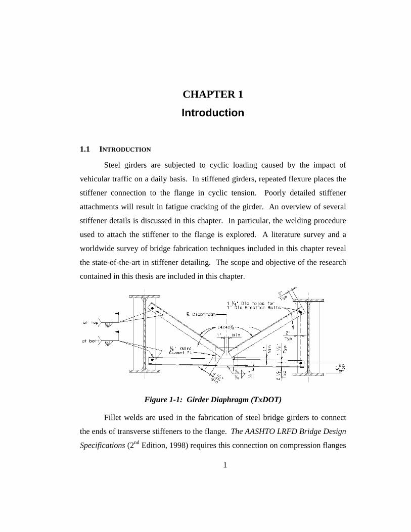
Figure 1-1: Girder Diaphragm (TxDOT)

Fillet welds are used in the fabrication of steel bridge girders to connect

the ends of transverse stiffeners to the flange. The AASHTO LRFD Bridge Design

Specifications (2nd Edition, 1998) requires this connection on compression flanges

1

to control distortion of the web-to-flange intersection. The stiffener must also be

connected to the tension flange when a cross frame or diaphragm is connected to

the stiffener. The diaphragms are typically attached to the stiffener as shown in

Figure 1-1. Diaphragms are mainly used during construction to provide lateral

bracing to the girder during the erection process. The stiffeners are run the full

depth of the girder web and are welded directly to the flanges. The lateral forces

from the diaphragm will cause fatigue cracks to form in the web at the end of

stiffener weld if the stiffener is not welded to the flange. Some states use a bolted

rather than a welded connection between the stiffener and the flange. Two angles

are welded to the stiffener and bolted to the flange. The two details are shown in

Figure 1-2.

Figure 1-2: Stiffener-to-Flange Connections

The welded detail is the preferred detail since it does not require

fabrication and fitup of the angles and the drilling of the flange bolt holes. The

Texas Department of Transportation (TxDOT) uses the welded detail.

Termination of the fillet welds at the end of the stiffener has been a subject of

much discussion. The present AASHTO welding specification does not require

the wrapping of the welds around the end of the stiffener. Historically, these

welds were required to be wrapped to seal the weld in order to prevent corrosion

2

at the interface of the stiffener and flange. Undercutting at the corner of the

stiffener often caused the wrapped welds to be rejected and subject to grinding to

feather out the undercut. The current specification language prohibits wrapping

of the welds to prevent the undercutting but leaves the ends of the stiffener

exposed to moisture. Some states require sealing of the ends with caulking,

which is difficult to perform and not a long-term solution. The current stiffener-

to-flange weld detail used by The Texas Department of Transportation is shown

in Figure 1-3.

Figure 1-3: Current Stiffener Weld Detail (TxDOT)

The influence of wrapping the weld upon fatigue performance was

evaluated through experimental testing at Ferguson Structural Engineering

Laboratory. Undercutting of the corners of stiffeners is unavoidable. In addition,

undercutting of the flange edge may occur if the width of the stiffener is large.

Undercuts at the corner of the flange are more likely to reduce fatigue

performance than undercuts of the stiffener. The impact of undercutting the

corners of the stiffener and flange upon fatigue performance were determined and

are presented in this thesis.

3

4

The wrapping of the welds at web side of the stiffener is difficult since it

must be performed through the clip. A large clip may be required to provide

access for the welder. A large clip reduces the amount of weld that can be placed

which may lead to weld failures from the cross frame forces. Elimination of the

clip and allowing the intersection of the stiffener and web-to-flange fillets welds

is a possible alternative. Testing of stiffener details with and without a clip were

conducted.

1.2 FABRICATION SURVEY

A recent Federal Highway Association sponsored worldwide survey of

steel bridge fabrication revealed that most countries wrapped the stiffener weld.

Findings from this survey are summarized in the FHWA report titled Steel Bridge

Fabrication Technologies in Europe and Japan (Verma et al, 2001). It was found

that other countries use a small clip on the stiffener and fill the void with weld

metal sealing the weld and eliminating the need to wrap the weld inside the clip.

A photograph of this stiffener detail is shown in Figure 1-4. Note that the weld is

also fully wrapped at the flange edge side of the stiffener and that good weld

profile was maintained with minimal undercutting.

Flange

WebStiffener

Filled Clip

Flange

WebStiffener

Filled Clip

Figure 1-4: Fully Wrapped Stiffener, No Clip

Intermediate and cross-frame stiffeners are shown on the girder in Figure

1-5. Fabricators wrapped the welds around the interior clip space near the web on

the diaphragm stiffener. The edge of the diaphragm stiffener near the flange was

also sealed. In addition, the stiffener-to-web weld of the intermediate stiffeners

was also wrapped around the top and bottom of the attachment.

5

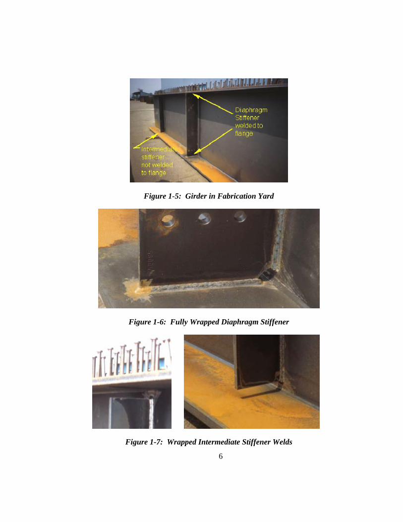
Figure 1-5: Girder in Fabrication Yard

Figure 1-6: Fully Wrapped Diaphragm Stiffener

Figure 1-7: Wrapped Intermediate Stiffener Welds

6

7

Figure 1-6 shows a close-up view of the diaphragm stiffener weld detail.

It can be seen from the figure that a circular “mouse hole” clip was used to fitup

the stiffener to the web. TxDOT uses a straight clip detail (refer to Figure 1-3).

Notice also that the weld shape and profile are maintained along the length of the

stiffener, including the wrapped edges. The holes shown in the stiffener are used

to bolt the diaphragm to the stiffeners during erection.

Figure 1-7 shows a close-up view of the intermediate stiffener weld detail.

The web-to-stiffener welds were carefully wrapped around the top and bottom

edges of the stiffener. It should be noted that the stiffeners were welded to the

web prior to the attachment of the flanges. The stiffener-to-flange weld shown in

Figure 1-6 was made last.

1.3 LITERATURE SURVEY

Ruge and Woesle tested three different stiffener details in cyclic four-point

bending at 11 Hz. The stiffener detail was located in the constant moment region

and tested at a stress range of 17 ksi (117 MPa) at the extreme fiber of the tension

flange. The stress range is defined as the difference between the upper and lower

stress limits at the extreme tension fiber during testing.

Figure 1-8: Specimen and Setup (Ruge and Woesle, 1962)

Figure 1-8 shows the specimen geometry and test setup used by Ruge and

Woesle. Dimensions are given in inches in Figure 1-8. Stiffener details A

through C were connected to the flange using 0.125 in. (3 mm) fillet welds.

Stiffener A has no interior clip opening, and welds were used to seal the stiffener

to the web and flange. It should be noted that the stiffener-to-flange weld did not

seal the interior stiffener clip for detail B. Ruge and Woesle indicate that stiffener

detail B is at a disadvantage since water can infiltrate between the stiffener and

flange leading to corrosion. However, detail C uses fully wrapped welds at the

interior clip region. Welds appear to be wrapped around the flange edge of the

stiffener for all specimens A through C.

8

It was reported that all cracks occurred along the toe of the stiffener-to-

flange weld. In addition, no cracks initiated at the web-to-flange weld in the

stiffened beams. Stiffener detail B was used to investigate the effects of crater

cracks on the fatigue performance of the beams. Ruge and Woesle concluded that

the crater cracks did not impact the fatigue life of the beams. Failure of the type

B stiffened beams occurred due to fatigue cracking at the toe of the stiffener-to-

flange weld.

Another significant conclusion drawn by the authors was that weld

sequence did not impact the fatigue performance of the specimens. The results of

the fatigue testing performed by Ruge and Woesle are perhaps the most

significant findings in relation to the research presented in this report. It will be

shown in Chapter 4 that the specimens tested at Ferguson Structural Engineering

Laboratory also failed due to crack growth at the toe of the stiffener-to-flange

welds.

Figure 1-9: Types of Undercuts (Petershagen, 1990)

The Influence of Undercut on the Fatigue Strength of Welds – A Literature

Survey (Petershagen, 1990) provides an in-depth discussion on the geometric

variables of undercuts at the toe of fillet welds and butt welds and their impact on

fatigue life. In the survey, an undercut is described as an “irregular groove along

9

the toe of a weld.” Petershagen adds that the undercuts are inherent in the

welding process and may occur in either the base or fill metal. Three

classifications of undercuts are shown in Figure 1-9. Type one undercuts are

referred to as “wide and curved.” Category two undercuts are “narrow”, and

category three undercuts are considered “micro-flaws”, with a depth less than

0.01 in. (0.25 mm). Category three undercuts are believed to be unavoidable

during welding and impossible to detect by visual inspection.

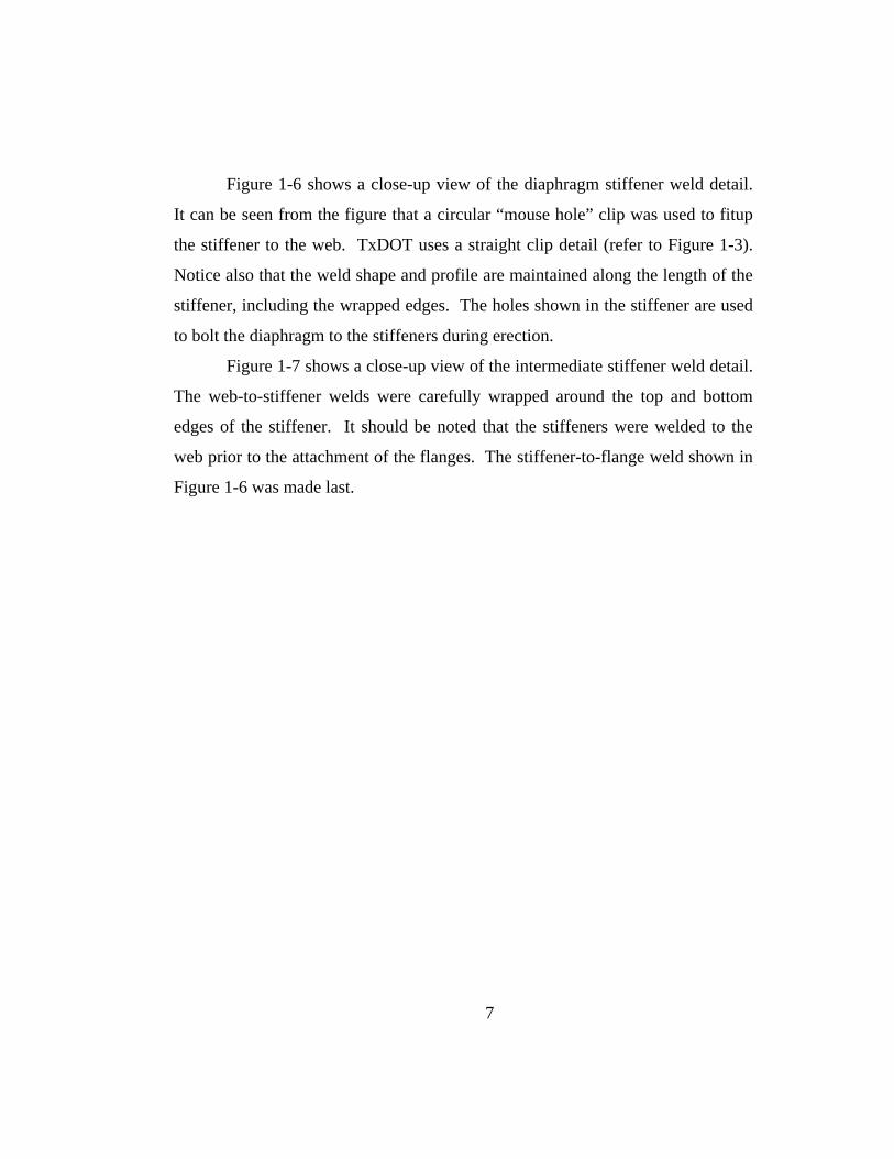
Petershagen’s survey also indicated that undercuts are generally

characterized by their length, height, and width. In addition, the transverse

orthogonal plane angel, ρ, and the notch root radius, r, were used to describe the

geometry of an undercut. Figure 1-10 illustrates several dimensions used to

represent the geometry of undercuts. However, it was found that only the length,

height, and direction of principal stresses are considered in AWS D1.1 and

German Shipbuilding Production Standard.

Figure 1-10: Undercut Dimensions (Petershagen, 1990)

Wrapping welds around gusset ends may increase the size of undercuts

(Petershagen, 1990). The author describes that wrapping fillet welds around non-

load bearing gussets attached to a plate yielded an average undercut height of 0.02

in. (0.49 mm). The unwrapped fillet weld produced average undercut depths of

0.006 in. (0.15 mm). Similar results may occur in the wrapping of stiffener-to-

10

11

flange welds around the edge of non-load bearing stiffeners connected to flange

plates.

Inspection of type one undercuts can be made using calipers or silicon

prints (Petershagen, 1990). Petershagen reports that type two undercuts are best

inspected using dye penetrant testing and magnetic particle testing. Type three

undercuts will also require the use of 250:1 scale microscopes. For the purposes

of the research conducted at Ferguson Structural Engineering Laboratory,

undercuts were exaggerated to produce “worst-case” undercuts. Thus, undercuts

were visible and measured using calipers to an accuracy of +0.005 inches.

Petershagen discusses the impact of undercuts on fatigue performance. It

was found that the fatigue life of welds with initial crack-like flaws could be

readily calculated using fracture mechanics equations. The fatigue life of welds

with type one or type two undercuts can also be determined. However,

Petershagen adds that no literature includes the simultaneous effects of type one,

two, and three undercuts.

Petershagen suggested that non-dimensional values, such as h/t (height-to-

thickness ratio), be used when describing undercuts. In addition, Petershagen

states that the crack initiation period is independent of the undercut depth, h. It

was also found that type one undercuts may cause a small impact on the fatigue

life of butt-welds, and that shape of fillet welds has a more significant impact on

fatigue life than undercutting (Petershagen, 1990).

Influence of the shape of undercut on the fatigue strength of fillet welded

assemblies – application of the local approach (Janosch and Debiez, 1998)

evaluated the impact of weld shape and continuous and discontinuous undercuts

at the fillet weld toe on fatigue strength. The authors state that the fatigue

resistance of structural details is based on nominal loads and plate thickness.

They add that design codes do not consider the fatigue strength as a function of

weld quality or undercutting.

Figure 1-11: T-Joint and Undercut Geometry (Janosch and Debiez, 1998)

Janosch and Debiez tested specimens welded by the manual and

MIG/MAG processes. Four weld undercutting geometries were examined: (1)

continuous undercuts at the upper toe by manual welding with covered electrodes

in the flat position; (2) discontinuous undercuts at the upper toe by manual

welding with covered electrodes in the flat position; (3) discontinuous undercuts

at both toes by manual welding with covered electrodes in the vertical upward

position; and (4) continuous undercuts at the upper toe by MIG/MAG welding

with solid wire in the flat position. T-shaped assemblies like the one shown in

Figure 1-11 were tested in four-point bending at 20 Hz to 40 Hz and a stress ratio

of 0.1. The stress ratio is defined as the minimum applied stress divided by the

maximum applied stress.

The geometry of the undercuts is also shown in Figure 1-11. The

undercuts are characterized by toe radius, ρ, and undercut depth, h. Table 1-1

shows the mean and standard deviation of these parameters per weld geometry 1

through 4 as measured by Janosch and Debiez.

12

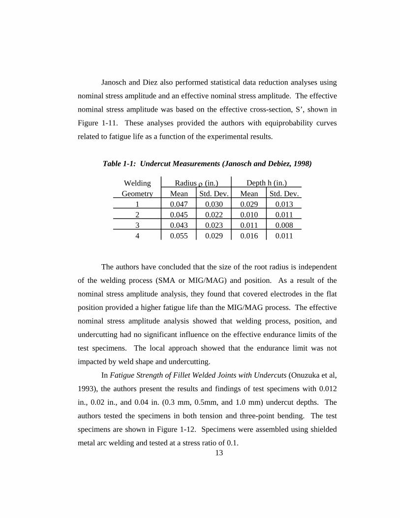
Janosch and Diez also performed statistical data reduction analyses using

nominal stress amplitude and an effective nominal stress amplitude. The effective

nominal stress amplitude was based on the effective cross-section, S’, shown in

Figure 1-11. These analyses provided the authors with equiprobability curves

related to fatigue life as a function of the experimental results.

Table 1-1: Undercut Measurements (Janosch and Debiez, 1998)

WeldingGeometry Mean Std. Dev. Mean Std. Dev.

1 0.047 0.030 0.029 0.0132 0.045 0.022 0.010 0.0113 0.043 0.023 0.011 0.0084 0.055 0.029 0.016 0.011

Radius ρ (in.) Depth h (in.)

The authors have concluded that the size of the root radius is independent

of the welding process (SMA or MIG/MAG) and position. As a result of the

nominal stress amplitude analysis, they found that covered electrodes in the flat

position provided a higher fatigue life than the MIG/MAG process. The effective

nominal stress amplitude analysis showed that welding process, position, and

undercutting had no significant influence on the effective endurance limits of the

test specimens. The local approach showed that the endurance limit was not

impacted by weld shape and undercutting.

13

In Fatigue Strength of Fillet Welded Joints with Undercuts (Onuzuka et al,

1993), the authors present the results and findings of test specimens with 0.012

in., 0.02 in., and 0.04 in. (0.3 mm, 0.5mm, and 1.0 mm) undercut depths. The

authors tested the specimens in both tension and three-point bending. The test

specimens are shown in Figure 1-12. Specimens were assembled using shielded

metal arc welding and tested at a stress ratio of 0.1.

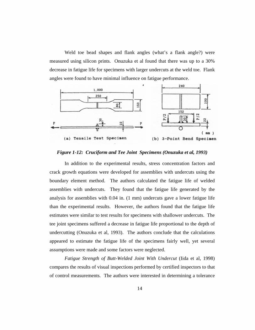
Weld toe bead shapes and flank angles (what’s a flank angle?) were

measured using silicon prints. Onuzuka et al found that there was up to a 30%

decrease in fatigue life for specimens with larger undercuts at the weld toe. Flank

angles were found to have minimal influence on fatigue performance.

Figure 1-12: Cruciform and Tee Joint Specimens (Onuzuka et al, 1993)

In addition to the experimental results, stress concentration factors and

crack growth equations were developed for assemblies with undercuts using the

boundary element method. The authors calculated the fatigue life of welded

assemblies with undercuts. They found that the fatigue life generated by the

analysis for assemblies with 0.04 in. (1 mm) undercuts gave a lower fatigue life

than the experimental results. However, the authors found that the fatigue life

estimates were similar to test results for specimens with shallower undercuts. The

tee joint specimens suffered a decrease in fatigue life proportional to the depth of

undercutting (Onuzuka et al, 1993). The authors conclude that the calculations

appeared to estimate the fatigue life of the specimens fairly well, yet several

assumptions were made and some factors were neglected.

Fatigue Strength of Butt-Welded Joint With Undercut (Iida et al, 1998)

compares the results of visual inspections performed by certified inspectors to that

of control measurements. The authors were interested in determining a tolerance

14

15

level for undercuts as judged by the certified inspectors. In particular, focus was

placed on finding an acceptable depth for undercutting. Butt-welded specimens

were also tested in fatigue and the authors reported that undercutting has an

impact on fatigue life.

0.8 in. (20 mm) butt welds and 0.5 in. (12 mm) fillet welds were used to

assemble the specimens using the shielded metal arc welding process (Iida et al,

1998). Weld gauges and silicon replicate prints were used to measure the

undercuts on the specimens. Next, over 100 certified inspectors were asked to

measure the same undercuts using a 0.1 mm pitch gauge. The inspectors were

directed to approve or disapprove by considering not just undercut depth, but

overall weld quality. The authors reported that the mean undercut depth

measured by the inspectors was lower than the control measurements made with

the weld gauge. The inspected butt weld undercuts were found to be 0.006 in.

(0.16 mm) smaller than the control measurements. Inspected fillet weld undercuts

were found to be 0.002 in. (0.06 mm) smaller than the control measurements. The

authors found an error range of +0.004 in. to –0.008 in. (+0.1 mm to –0.2 mm) in

measured versus inspected undercut depths. In addition, the authors report that

most of the inspectors considered a 0.008 in. (0.2 mm) undercut to be acceptable

and a 0.04 in. (1.0 mm) undercut to be unacceptable.

Fatigue tests of butt-welded specimens with undercuts were performed at a

frequency of 5 Hz to10 Hz at a zero stress ratio in tension. Specimens with 0.63

in., 1.2 in., and 1.6 in. (16 mm, 30 mm, and 40 mm) plate thickness values were

tested. Results showed that the fatigue life decreased with undercut depth. In

particular, as the ratio of undercut depth to plate thickness (d/t) increases, the

fatigue life decreases. The authors reported a 5%, 10%, and 20% decrease in

fatigue life related to d/t ratios of 0.005, 0.01, and 0.02.

Iida et al concluded that inspectors underestimated the undercut depths. In

addition to finding that larger d/t ratios reduce fatigue life, the authors added that

the decrease was more prominent in thicker plates. The authors proposed the

following guidelines for the acceptance of undercuts in butt welds: (1) d < 0.2 mm

for t < 10 mm; (2) d/t < 0.02 for 10 mm < t < 40 mm; (3) d < 0.8 mm for t > 40

mm. The authors believed that using a weld gauge was the best way to measure

undercut depths because of the simplicity of the device.

Figure 1-13: Transverse and Longitudinal Specimens (Gurney, 1968)

Methods used to improve the fatigue life of fillet-welded assemblies are

discussed in Effect of Peening and Grinding on the Fatigue Strength of Fillet

Welded Joints (Gurney, 1968). Peening and grinding effects at the ends of

transverse and longitudinal fillet welds are investigated using the specimens

shown in Figure 1-13. The main plate of the specimens was 0.5 in. in thickness.

Peening, partial grinding of the weld toe, and full grinding of the weld were

carried out. Specimens were manually welded using E 317 rutile electrodes in the

flat position. Welds were fully wrapped around the edge of specimens with

longitudinal gussets in some cases. Welds were not wrapped around the edge of

the specimens with transverse gussets. Cyclic loading of the specimens took

place at a frequency of 3 Hz to 33 Hz and a stress ratio of either 0.0 or -1.0.

16

17

Three test machines were used, thus accounting for this variation in frequency and

stress ratio.

Gurney concluded that the fatigue performance of the specimens with

longitudinal gussets with wrapped welds were the same as for those with

unwrapped welds. However, the author adds that there was a particular case

where this was not so. Gurney states that a specimen with a longitudinal gusset

and wrapped welds failed earlier than the unwrapped gussets. Gurney mentioned

that this was due to an undercut at the toe of the weld wrap. Failures of the

longitudinal gussets occurred at the weld root. Full-penetration welds were then

tested and it was shown that an increase in fatigue strength occurred. However,

Gurney also noted that poor quality full penetration welds at the end of the gusset

plate could severely decrease fatigue life.

It was found that full grinding of the transverse welds resulted in a 50%

increase in fatigue performance. Light grinding was shown to produce mixed

results. The author believed that, while fatigue strength increased in some cases,

the ability to reproduce the desired light grinding was unreliable. Light grinding

depths could be too deep or too shallow and were considered inconsistent. In

addition, when fully ground specimens were also peened, a further increase in

fatigue performance was shown.

On the Practical Use of Weld Improvement Methods (Nussbaumer and

Imhof, 2001) investigates the influence of weld grinding, remelting, and peening.

These improvements are applied to the weld toe of welded assemblies to improve

their overall fatigue performance. The authors develop adjustments that account

for these weld improvements that can be applied to the nominal fatigue resistance

categories of Eurocode 3. It was stated that the weld improvements were

influenced by the stress ratio, R, and that the corrections work best for low stress

ratio values. Although undercuts can be removed by grinding, good weld quality

was also emphasized in order to produce a satisfactory fatigue performance.

Nussbaumer and Imhof believe that grinding, peening, and remelting of welds

using a TIG torch can not only be applied to new fabrications, but to structures

exhibiting cracking less than 2 mm in depth.

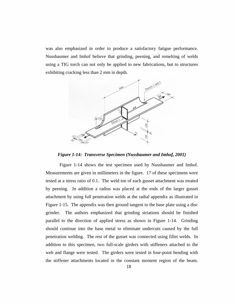
Figure 1-14: Transverse Specimen (Nussbaumer and Imhof, 2001)

18

Figure 1-14 shows the test specimen used by Nussbaumer and Imhof.

Measurements are given in millimeters in the figure. 17 of these specimens were

tested at a stress ratio of 0.1. The weld toe of each gusset attachment was treated

by peening. In addition a radius was placed at the ends of the larger gusset

attachment by using full penetration welds at the radial appendix as illustrated in

Figure 1-15. The appendix was then ground tangent to the base plate using a disc

grinder. The authors emphasized that grinding striations should be finished

parallel to the direction of applied stress as shown in Figure 1-14. Grinding

should continue into the base metal to eliminate undercuts caused by the full

penetration welding. The rest of the gusset was connected using fillet welds. In

addition to this specimen, two full-scale girders with stiffeners attached to the

web and flange were tested. The girders were tested in four-point bending with

the stiffener attachments located in the constant moment region of the beam.

Some of the findings in the work by Nussbaumer and Imhof coincide with the

fabrication of the specimen used for the research in this report. It will be shown

that the test specimen discussed in Chapter 2 is similar to the test specimen used

by Nussbaumer and Imhof.

Figure 1-15: Fabrication of Specimen Taper (Nussbaumer and Imhof, 2001)

Nussbaumer and Imhof also suggested that care should be taken at the

startup and termination points of the fillet welds. This concept is also discussed

in Fatigue of Welded Structures, 2nd Edition (Gurney, 1979). Gurney states that

termination points in otherwise continuous welds should be ground to a smooth

transition and then rewelded. This process is shown in Figure 1-16. Weld start-

stop regions are discussed in the following chapter for the fabrication of the test

specimens presented in this thesis. Weld start-stop repairs were made by grinding

and remelting by a TIG torch.

19

Figure 1-16: Weld Start-Stop Repair (Gurney, 1979)

Nussbaumer and Imhof concluded that design curves could be adjusted

using the formulation presented in their work. The authors also emphasized the

importance of quality control during welding, namely the weld quality and

procedure. They state that the application of the repair procedures should be done

so with care and precision. Nussbaumer and Imhof reported that peening

improves fatigue strength when lower stress ratios are used.

20

21

1.4 SCOPE OF WORK

Limited testing has been conducted on the fatigue strength of stiffeners

with undercuts. The literature survey reveals that the focus of research has been

on undercutting at the weld toe, and not at the stiffener and flange edge weld wrap

locations.

The impact of wrapping the stiffener-to-flange weld upon fatigue life was

evaluated and the results are presented in the following chapters. Several test

specimens were developed. The fabrication and design of the test specimens are

covered in Chapter 2 of this thesis. Undercuts were measured and the values are

presented.

Specimens were subjected to cyclic loading in tension. The test apparatus

and test procedure are discussed in chapter 3. Strain readings were also compared

to a finite element model used in the development of the test specimen. The

results of the fatigue tests are given in Chapter 4. Photographs of fatigue cracks

and fracture surfaces are included. A data analysis was also performed and

included in Chapter 4.

The conclusions of the research presented in this thesis are discussed in

Chapter 5. It was found that wrapping the welds around the stiffener had no

impact upon the fatigue life of the specimens.

22

CHAPTER 1 Introduction ........................................................................... 1

1.1 Introduction ................................................................................. 1

1.2 Fabrication Survey ...................................................................... 5

1.3 Literature Survey ......................................................................... 8

1.4 Scope of Work ........................................................................... 21

Table 1-1: Undercut Measurements (Janosch and Debiez, 1998) ........................ 13

Figure 1-1: Girder Diaphragm (TxDOT) ............................................................... 1

Figure 1-2: Stiffener-to-Flange Connections ......................................................... 2

Figure 1-3: Current Stiffener Weld Detail (TxDOT) ............................................. 3

Figure 1-4: Fully Wrapped Stiffener, No Clip ....................................................... 5

Figure 1-5: Girder in Fabrication Yard .................................................................. 6

Figure 1-6: Fully Wrapped Diaphragm Stiffener ................................................... 6

Figure 1-7: Wrapped Intermediate Stiffener Welds ............................................... 6

Figure 1-8: Specimen and Setup (Ruge and Woesle, 1962) .................................. 8

Figure 1-9: Types of Undercuts (Petershagen, 1990) ............................................ 9

Figure 1-10: Undercut Dimensions (Petershagen, 1990) ..................................... 10

Figure 1-11: T-Joint and Undercut Geometry (Janosch and Debiez, 1998) ........ 12

Figure 1-12: Cruciform and Tee Joint Specimens (Onuzuka et. all, 1993)......... 14

Figure 1-13: Transverse and Longitudinal Specimens (Gurney, 1968) ............... 16

Figure 1-14: Transverse Specimen (Nussbaumer and Imhof, 2001) ................... 18

Figure 1-15: Fabrication of Specimen Taper (Nussbaumer and Imhof, 2001) .... 19

Figure 1-16: Weld Start-Stop Repair (Gurney, 1979) .......................................... 20

CHAPTER 2 Specimen Design and Fabrication

2.1 INTRODUCTION

The specimens tested during the project are introduced in this chapter.

This chapter describes the design process used for the development of the test

specimen. Fabrication of each specimen group is covered in detail.

Figure 2-1 shows a steel girder subjected to flexure. The stiffener is

welded to both flanges and along the web. Repeated flexure of the girder places

the stiffener-to-flange connection under cyclic tensile loading. The stiffener-to-

flange detail is highlighted with a circle in the section figure.

X

X Section X-X

Flange

Stiffener

Web

Figure 2-1: Steel Girder and Stiffener Detail Under Flexural Loading

An axially loaded test specimen was used to simulate the tensile stresses in

the flange due to girder flexure. The test specimen is shown in Figure 2-2. The

22

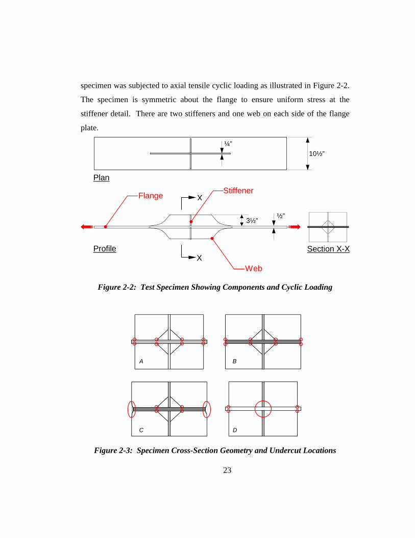
specimen was subjected to axial tensile cyclic loading as illustrated in Figure 2-2.

The specimen is symmetric about the flange to ensure uniform stress at the

stiffener detail. There are two stiffeners and one web on each side of the flange

plate.

23

Stiffener Flange

Web

X

X

Section X-X

¼”10½”

Plan

Profile

½”3½”

Figure 2-2: Test Specimen Showing Components and Cyclic Loading

A

C D

B

Figure 2-3: Specimen Cross-Section Geometry and Undercut Locations

Four different types of specimens were used to investigate the possible

effects of the undercutting caused by wrapping the fillet welds around the

stiffener. These specimens, designated type A through type D, were designed to

evaluate the fatigue performance based on undercutting at the interior stiffener

clip weld wrap and undercutting at the edge of the stiffener-to-flange weld.

Figure 2-3 illustrates the cross-section geometry at the stiffener-to-flange

connection. Undercut locations and other points of interest are highlighted with

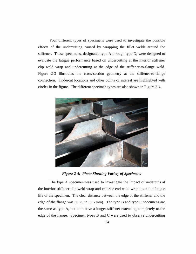
circles in the figure. The different specimen types are also shown in Figure 2-4.

Figure 2-4: Photo Showing Variety of Specimens

The type A specimen was used to investigate the impact of undercuts at

the interior stiffener clip weld wrap and exterior end weld wrap upon the fatigue

life of the specimen. The clear distance between the edge of the stiffener and the

edge of the flange was 0.625 in. (16 mm). The type B and type C specimens are

the same as type A, but both have a longer stiffener extending completely to the

edge of the flange. Specimen types B and C were used to observe undercutting

24

25

effects at the interior clip weld wrap and the stiffener-to-flange edge weld wrap.

The type C specimen is identical to type B with the exception that the flange edge

undercut was removed by grinding after fabrication in accordance with section

3.2.3 of the D1.5-95 Bridge Welding Code (1995). Lastly, the type D specimen

was used to investigate the impact on the fatigue life caused by minimizing the

clip size and completely welding this area closed. The clear distance between the

edge of the stiffener and the edge of the flange was 0.625 in. (16 mm) for type D

specimens.

AASHTO LRFD Bridge Design Specifications, 2nd Edition (1998)

nominal fatigue resistance categories were employed in the design of the

specimens based on a nominal stress range, SR, of 20 ksi (138 MPa) at the

stiffener-to-flange connection. The design ensured that failure of the specimens

occurred at either the undercuts or the weld at the stiffener location. The

specimens were designed to avoid premature fatigue failure at a location other

than at the stiffener detail.

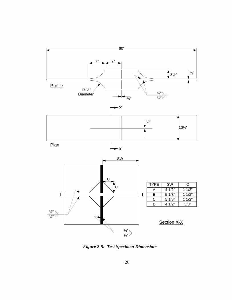
Figure 2-5 shows the dimensions of specimens A, B, C, and D. All

specimens were 60 in. long (1524 mm) and had a flange thickness of 0.5 in. (12.7

mm). The stiffener and web plates were each 0.25 in. thick (6.35 mm). The table

in Figure 2-5 lists the stiffener width and clip size for each specimen type. The

clip is the triangular opening on the stiffener nearest to the web-to-flange weld.

The stiffener widths were either 4.5 in. (114 mm) or 5.125 in. (130 mm) and the

clip sizes were either 1.5 in. (38 mm) or 0.375 in. (9.5 mm). The specimens were

welded using the gas metal arc welding (GMAW) process with a metal-cored

electrode. The specimens were assembled using 0.25 in. welds (6.35 mm). The

web sections were ground smooth at the ends using a disk grinder to eliminate

fatigue cracking at the termination of the weld. The surface grinding marks were

finished parallel with the direction of loading.

Plan

X

X

10½”¼”

Profile

7” 7”

3½” ½”

17 ½” Diameter

¼” ¼” ¼”

60”

Section X-X

TYPE SW CA 4 1/2" 1 1/2"B 5 1/8" 1 1/2"C 5 1/8" 1 1/2"D 4 1/2" 3/8"

¼” ¼”

¼” ¼”

SW

C

C

Figure 2-5: Test Specimen Dimensions

26

2.2 SPECIMEN DESIGN

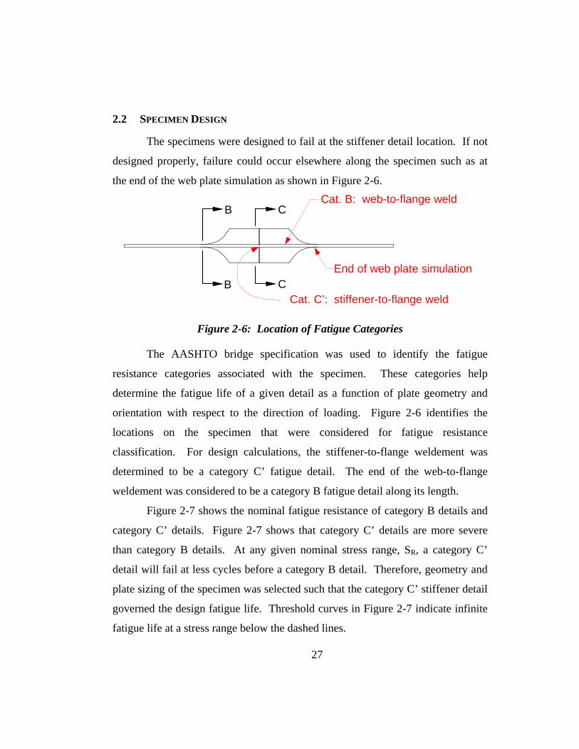
The specimens were designed to fail at the stiffener detail location. If not

designed properly, failure could occur elsewhere along the specimen such as at

the end of the web plate simulation as shown in Figure 2-6.

C

C

B

B

Cat. B: web-to-flange weld

Cat. C’: stiffener-to-flange weld

End of web plate simulation

Figure 2-6: Location of Fatigue Categories

The AASHTO bridge specification was used to identify the fatigue

resistance categories associated with the specimen. These categories help

determine the fatigue life of a given detail as a function of plate geometry and

orientation with respect to the direction of loading. Figure 2-6 identifies the

locations on the specimen that were considered for fatigue resistance

classification. For design calculations, the stiffener-to-flange weldement was

determined to be a category C’ fatigue detail. The end of the web-to-flange

weldement was considered to be a category B fatigue detail along its length.

Figure 2-7 shows the nominal fatigue resistance of category B details and

category C’ details. Figure 2-7 shows that category C’ details are more severe

than category B details. At any given nominal stress range, SR, a category C’

detail will fail at less cycles before a category B detail. Therefore, geometry and

plate sizing of the specimen was selected such that the category C’ stiffener detail

governed the design fatigue life. Threshold curves in Figure 2-7 indicate infinite

fatigue life at a stress range below the dashed lines.

27

1

10

100

1.0E+05 1.0E+06 1.0E+07 1.0E+08

Number of Cycles, Nf

Stre

ss R

ange

, S R

(K

SI)

Category C' Category B Category C' Threshold Category B Threshold

Figure 2-7: AASHTO Nominal Fatigue Resistance Categories B & C’

ff b t Area ×=Section C-C Section B-B

tw

tf d

bf

tf

bf

( ) ( )ffw bt dt 2 Area ⋅+⋅×=

Figure 2-8: Area Used For Calculating Nominal Stress

28

All specimens were tested under cyclic loading at a nominal stress range,

SR, of 20 ksi (138 MPa) at section C-C shown in Figures 2-6 and 2-8. The stress

range is the difference between the minimum and maximum nominal stresses.

The minimum and maximum nominal stresses across section C-C were 5 ksi (34.5

MPa) and 25 ksi (172 MPa), respectively. These nominal stresses were calculated

by dividing the applied axial load on the specimen by the area of the web and

flange plates shown in Figure 2-8, Section C-C. The lower stress limit

corresponded to an axial load of 35 kips (156 kN), whereas the upper stress limit

was produced by an axial load of 175 kips (778 kN). It should be noted that the

stress range at section B-B shown in Figures 2-6 and 2-8 is higher than the stress

range at section C-C due to the decrease in area. The stress range at section B-B

is 26.7 ksi (184 MPa).

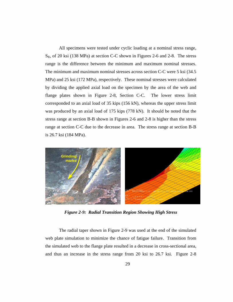
Grindingmarks

Figure 2-9: Radial Transition Region Showing High Stress

The radial taper shown in Figure 2-9 was used at the end of the simulated

web plate simulation to minimize the chance of fatigue failure. Transition from

the simulated web to the flange plate resulted in a decrease in cross-sectional area,

and thus an increase in the stress range from 20 ksi to 26.7 ksi. Figure 2-8

29

30

illustrates this difference between these cross-sectional areas. Additionally, a

finite element model discussed in the following section shows that high principal

stresses exist at the radial taper in Figure 2-9. The radial taper created a high

stress concentration at the end of the web. Defined as the maximum principal

stress divided by the nominal stress, the stress concentration factor at the end of

the taper was approximately 1.2. The transition region was grinded flush to the

flange plate using a disk grinder and belt sander to minimize the increase in stress

and to eliminate any discontinuities from the welds. Thus, the fatigue

performance of the taper transition was estimated as a category B detail. The

required flange and web sizes were determined based on the nominal fatigue

resistance of the stiffener-to-flange connection in comparison to the web-to-flange

weldement. The final plate sizing satisfies the fatigue resistance demands such

that specimen failure is constrained to the stiffener-to-flange connection.

The specimen was designed to make the stiffener-to-flange weld control

the fatigue life of the specimen. The ratio of area B-B to area C-C (refer to Figure

2-8) was determined to prevent a fatigue failure at the radiussed end of the web-

to-flange weld.

The test specimen design calculations that produce the desired failure are

now presented. The predicted fatigue life of the stiffener-to-flange detail is

550,000 cycles at a nominal stress range of 20 ksi (138 MPa). The predicted

fatigue life of the web-to-flange weld toe at the end of the web simulation (refer

to Figure 2-6) is 632,575 cycles at a nominal stress range of 26.7 ksi (184 MPa).

All stresses were kept within the capacity of the actuator and test frame to be

discussed in Chapter 3 of this report.

31

( ) ( )( ) ( )

( ) ( ) ( ) ( )

( ) ( ) ( ) dt2tbP S

tbP S

: as sectionscategory respective at the range stress theexpress toused are 8-2 Figurein shown areas The

S1.40 S or0.716 SS

therefore,S1044 S10120

N NC'category stiffener, at the life fatigue than the

greater bemust B,category weld,flange-to- web theof end at the life fatigue TheS1044 N

S10120 N

So,AS N

follows, as calculated is life fatigue The1044 A

10120 Aare C and Bfor constantscategory detailion specificat bridge AASHTO From

kips range, load Pksi range, stress S

constantcategory detail A failure tocycles N

in. , thickness web tin. height,stiffener d

in. , thicknessflange tin. width,flange b

:reNomenclatu

wff

RRC

ff

RRB

RCRBRB

RC

3-RC

83-RB

8

CB

3-RC

8C

3-RB

8B

3-R

8C

8B

R

R

w

f

f

⋅⋅+⋅=

⋅=

⋅<>

⋅×>⋅×

>

⋅×=

⋅×=

=

×=

×=

========

( ) ( )

( ) ( )

( ) ( )[ ]

( ) ( )[ ]

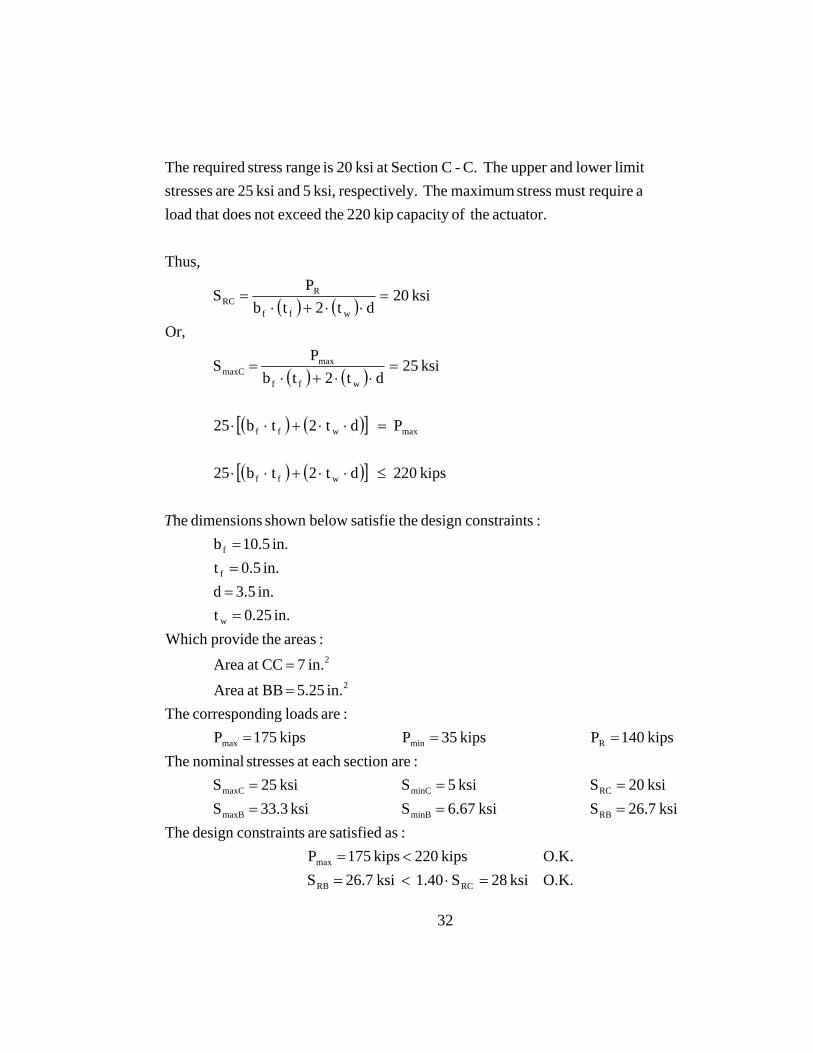
O.K.ksi 28 S1.40 ksi 26.7 SO.K.kips 220 kips 175 P

:as satisfied are sconstraintdesign Theksi 26.7 Sksi 6.67 Sksi 33.3 S

ksi 20 Sksi 5 Sksi 25 S :aresection each at stresses nominal The

kips 140 Pkips 35 Pkips 175 P:are loads ingcorrespond The

in. 5.25 BBat Areain. 7 CCat Area

:areas theprovideWhich in. 0.25 t

in. 3.5 din. 0.5 t

in. 10.5 b :sconstraintdesign thesatisfie belowshown dimensions he

kips 220 dt2tb25

P dt2tb25

ksi 25dt2tb

P S

Or,

ksi 20dt2tb

P S

Thus,

actuator. theofcapacity kip 220 theexceednot does that loada requiremust stress maximum The ly.respective ksi, 5 and ksi 25 are stresses

limitlower andupper The C.-CSection at ksi 20 is range stress required The

RCRB

max

RBminBmaxB

RCminCmaxC

Rminmax

2

2

w

f

f

wff

maxwff

wff

maxmaxC

wff

RRC

=⋅<=<=

======

===

=

=

====

≤⋅⋅+⋅⋅

=⋅⋅+⋅⋅

=⋅⋅+⋅

=

=⋅⋅+⋅

=

T

32

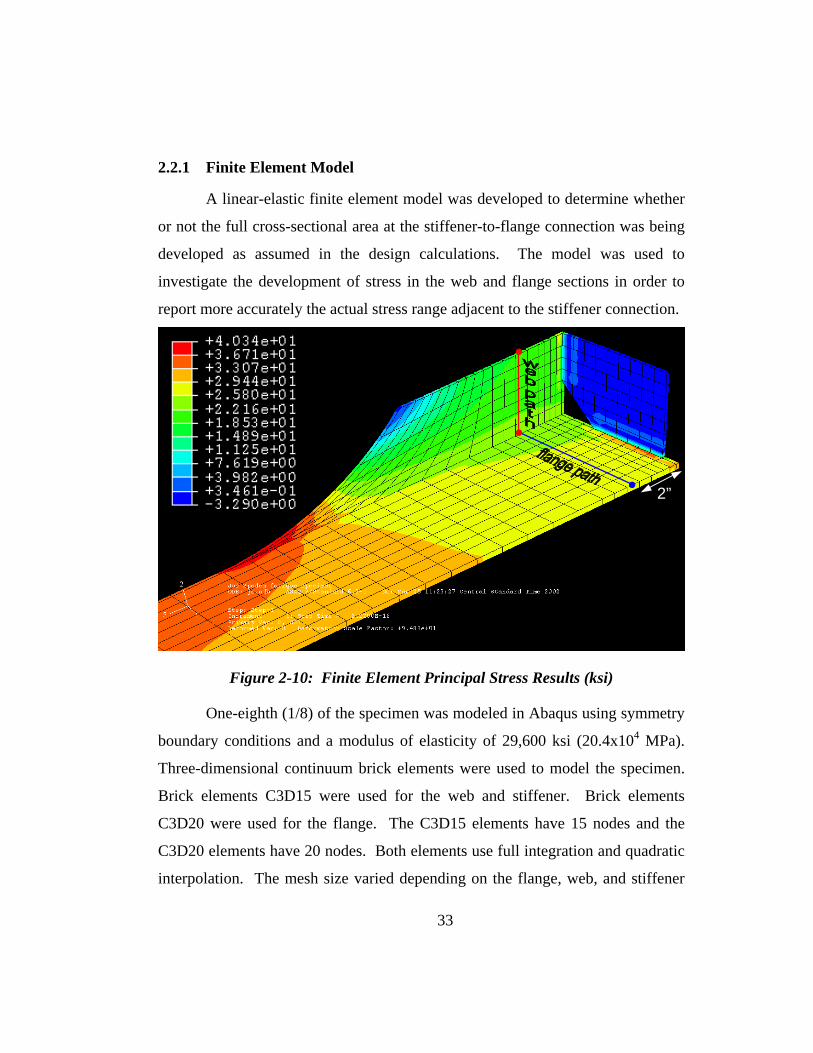
2.2.1 Finite Element Model

A linear-elastic finite element model was developed to determine whether

or not the full cross-sectional area at the stiffener-to-flange connection was being

developed as assumed in the design calculations. The model was used to

investigate the development of stress in the web and flange sections in order to

report more accurately the actual stress range adjacent to the stiffener connection.

2”

Figure 2-10: Finite Element Principal Stress Results (ksi)

One-eighth (1/8) of the specimen was modeled in Abaqus using symmetry

boundary conditions and a modulus of elasticity of 29,600 ksi (20.4x104 MPa).

Three-dimensional continuum brick elements were used to model the specimen.

Brick elements C3D15 were used for the web and stiffener. Brick elements

C3D20 were used for the flange. The C3D15 elements have 15 nodes and the

C3D20 elements have 20 nodes. Both elements use full integration and quadratic

interpolation. The mesh size varied depending on the flange, web, and stiffener

33

34

components being modeled. A small mesh of 0.25 in. long by 0.5 in. wide (6.35

mm by 12.7 mm) elements was used for the flange and web near the stiffener over

a length of approximately 1.0 in. (25.4 mm). The length of the flange and web

elements increased further away from the stiffener in the longitudinal direction,

and the width remained constant perpendicular to the direction of loading. The

flange and web element thickness were 0.25 in. (6.35 mm) and 0.125 in. (3.2

mm), respectively. 0.5 in. long by 0.5 in. wide by 0.125 in. thick (12.7 mm by

12.7 mm by 3.2 mm) elements were used for the stiffener.

Figure 2-10 shows the results of the finite element analysis. Recall that

the nominal upper limit stress at the stiffener-to-flange connection is 25 ksi (172

MPa). The stresses shown in Figure 2-10 caused by the maximum static load of

175 kips (778 kN) were generated in Abaqus by applying a uniformly distributed

tensile load at the plate end (gripped portion of specimen). The analysis shows

that the stress in the flange plate was higher than the stress in the web plate.

A flange path and a web path are shown in Figure 2-10. The paths are

located at the same distance from the stiffener as strain gages discussed in

Chapter 3.3.2.2. It should be noted that a higher value of stress exists

immediately adjacent to the stiffener-to-flange weld toe as shown in Figure 2-10.

This stress is approximately 33 ksi (228 MPa) at maximum applied load, and this

stress increase is due to the abrupt change in geometry caused by the stiffener

detail.

Figure 2-11 shows a plot of principal stress along the flange surface

corresponding to the “flange path” labeled in Figure 2-10. A maximum stress of

approximately 27.3 ksi (188 MPa) occurs near the edge of the flange. A

minimum stress of 23.8 ksi (164 MPa) occurs at the web connection. The average

upper limit stress in the flange is 26.2 ksi (181 MPa).

23.5

24.0

24.5

25.0

25.5

26.0

26.5

27.0

27.5

0 1 2 3 4 5

Distance From Web Centerline (in.)

Prin

cipa

l Str

ess

(ksi

)

Figure 2-11: Principal Stress Along Flange Path

0.0

0.5

1.0

1.5

2.0

2.5

3.0

3.5

18 19 20 21 22 23 24

Principal Stress (ksi)

Figure 2-12: Principal Stress Along Web Path

35

36

Figure 2-12 shows a plot of principal stress along the web centerline

corresponding to the “web path” depicted in Figure 2-10. The maximum stress of

approximately 23.8 ksi (164 MPa) occurs at the flange connection. A minimum

stress of approximately 18.7 ksi (129 MPa) occurs at the top of the web plate.

The average upper limit stress in the web is 21.1 ksi (145 MPa).

The results of the finite element model showed that the stress was not

uniform near the stiffener section. In particular, stress in the web was not fully

developed. The largest web stress was less than the nominal upper limit stress of

25 ksi (172 MPa). Stress in the flange edge was higher than the stress at the

flange centerline. Stresses reported in the flange will directly influence the

fatigue life of the stiffener-to-flange connection. The larger stress at the flange

edge will reduce the fatigue life at the flange edge.

The average principal stress in the flange under the 175 kip maximum

loading condition was determined to be 26.2 ksi (181 MPa). Under the 35 kip

minimal loading condition, the principal stress is [ 35/175 ] x 26.2 ksi, or 5.24 ksi

(36.1 MPa) with a resulting stress range of 21 ksi (145 MPa) in the flange.

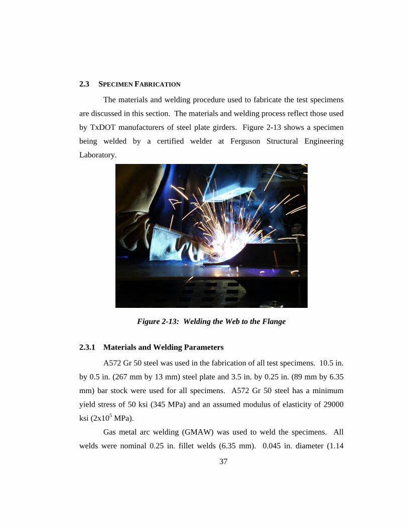
2.3 SPECIMEN FABRICATION

The materials and welding procedure used to fabricate the test specimens

are discussed in this section. The materials and welding process reflect those used

by TxDOT manufacturers of steel plate girders. Figure 2-13 shows a specimen

being welded by a certified welder at Ferguson Structural Engineering

Laboratory.

Figure 2-13: Welding the Web to the Flange

2.3.1 Materials and Welding Parameters

A572 Gr 50 steel was used in the fabrication of all test specimens. 10.5 in.

by 0.5 in. (267 mm by 13 mm) steel plate and 3.5 in. by 0.25 in. (89 mm by 6.35

mm) bar stock were used for all specimens. A572 Gr 50 steel has a minimum

yield stress of 50 ksi (345 MPa) and an assumed modulus of elasticity of 29000

ksi (2x105 MPa).

Gas metal arc welding (GMAW) was used to weld the specimens. All

welds were nominal 0.25 in. fillet welds (6.35 mm). 0.045 in. diameter (1.14

37

mm) FabCOR 86R E70C-6M metal-cored electrode wire was used with a travel

speed of approximately 16 IPM and a wire speed of 310 IPM. The machine was

set to 200 amps at 26 volts. The shielding gas was a mixture of 90% Argon and

10% CO2.

2.3.2 Assembly

Figure 2-14 shows several A572 Gr 50 steel flange, web, and stiffener

parts used for the specimens prior to welding. Stiffener and flange undercuts

were intentionally created during the welding process to produce worst-case

scenarios.

Figure 2-14: Steel Parts Prior to Welding

The 0.5 in. thick (13mm) flange used for the specimen was cut from 120

in. by 10.5 in. (3048 mm by 267 mm) plates using a band saw. The 0.25 in. thick

(6.4 mm) web and stiffener parts were cut from 240 in. by 3.5 in. (6096 mm by 89

mm) bar stock using a band saw. The web section radius was then cut using a

plasma torch.

38

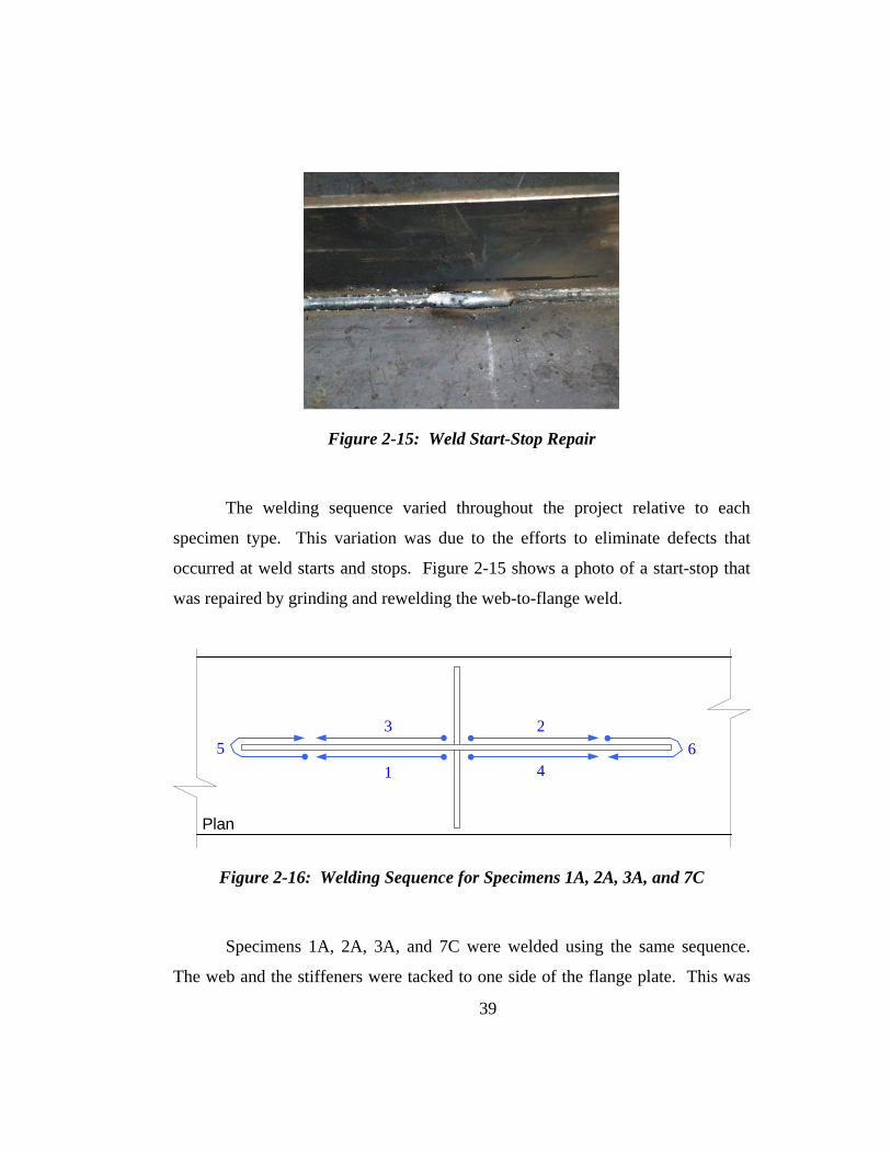
Figure 2-15: Weld Start-Stop Repair

The welding sequence varied throughout the project relative to each

specimen type. This variation was due to the efforts to eliminate defects that

occurred at weld starts and stops. Figure 2-15 shows a photo of a start-stop that

was repaired by grinding and rewelding the web-to-flange weld.

Plan

1

3

46

25

Figure 2-16: Welding Sequence for Specimens 1A, 2A, 3A, and 7C

Specimens 1A, 2A, 3A, and 7C were welded using the same sequence.

The web and the stiffeners were tacked to one side of the flange plate. This was

39

next repeated on the opposite side. Welds were then made in the horizontal

position in the sequence illustrated in Figure 2-16. The stiffeners were next

welded to the flange in the horizontal position starting from the interior clip,

continued around the stiffener edge, and back to the clip. In some cases, the weld

was stopped midway between the stiffener edge and clip. A short pass was then

used to complete the weld seal. This was done on both stiffeners on the top

surface of the flange and then repeated on the opposite surface. The stiffeners

were then welded to the web in the horizontal position.

Plan

1

3

24

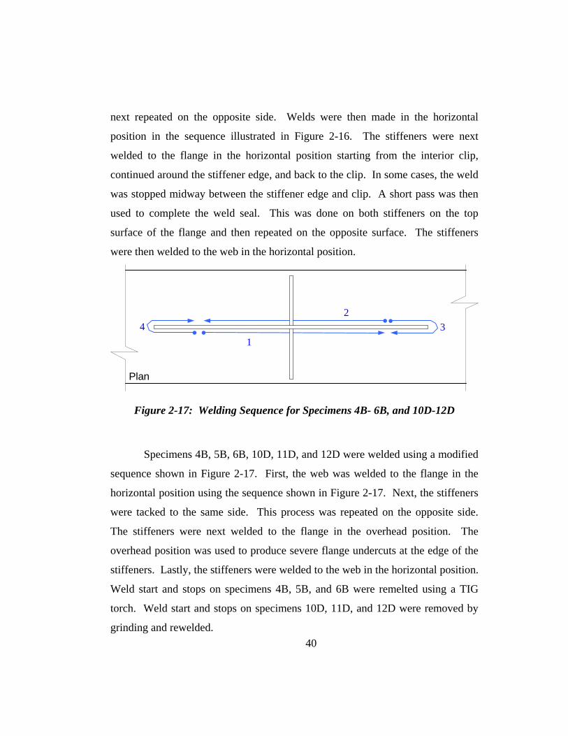
Figure 2-17: Welding Sequence for Specimens 4B- 6B, and 10D-12D

Specimens 4B, 5B, 6B, 10D, 11D, and 12D were welded using a modified

sequence shown in Figure 2-17. First, the web was welded to the flange in the

horizontal position using the sequence shown in Figure 2-17. Next, the stiffeners

were tacked to the same side. This process was repeated on the opposite side.

The stiffeners were next welded to the flange in the overhead position. The

overhead position was used to produce severe flange undercuts at the edge of the

stiffeners. Lastly, the stiffeners were welded to the web in the horizontal position.

Weld start and stops on specimens 4B, 5B, and 6B were remelted using a TIG

torch. Weld start and stops on specimens 10D, 11D, and 12D were removed by

grinding and rewelded. 40

Plan

1

2

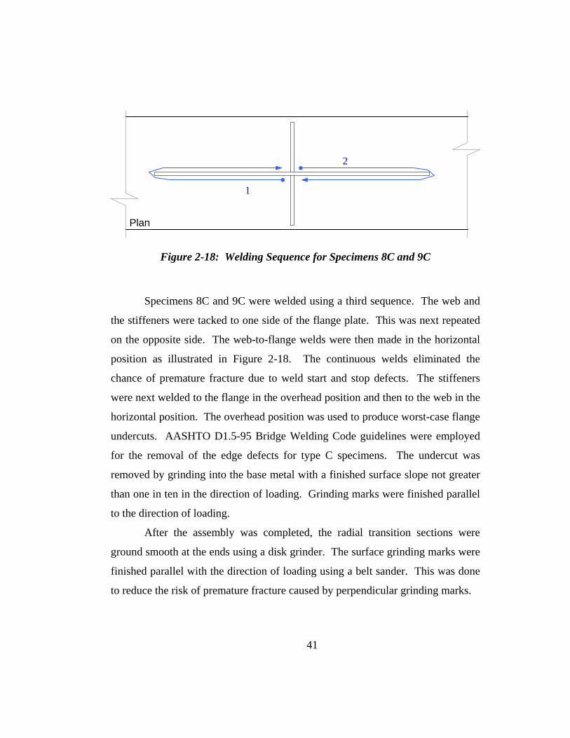
Figure 2-18: Welding Sequence for Specimens 8C and 9C

Specimens 8C and 9C were welded using a third sequence. The web and

the stiffeners were tacked to one side of the flange plate. This was next repeated

on the opposite side. The web-to-flange welds were then made in the horizontal

position as illustrated in Figure 2-18. The continuous welds eliminated the

chance of premature fracture due to weld start and stop defects. The stiffeners

were next welded to the flange in the overhead position and then to the web in the

horizontal position. The overhead position was used to produce worst-case flange

undercuts. AASHTO D1.5-95 Bridge Welding Code guidelines were employed

for the removal of the edge defects for type C specimens. The undercut was

removed by grinding into the base metal with a finished surface slope not greater

than one in ten in the direction of loading. Grinding marks were finished parallel

to the direction of loading.

After the assembly was completed, the radial transition sections were

ground smooth at the ends using a disk grinder. The surface grinding marks were

finished parallel with the direction of loading using a belt sander. This was done

to reduce the risk of premature fracture caused by perpendicular grinding marks.

41

2.4 DETAILS OF WELD UNDERCUTS

Undercuts were intentionally produced during the fabrication of the type

A, B, C, and D specimens. Attempts were made to create the largest undercut

possible to produce worst-case scenarios. Undercut locations and characteristics

are discussed in this section for all specimens.

Type A specimens were used to investigate the influence of undercutting

on the fatigue performance caused by wrapping the stiffener weld around the

interior clip and exterior edges of the stiffener. A close-up of the type A stiffener

detail is shown in Figure 2-19. Arrows are used in the figure to indicate the

points of undercutting.

C

C

Figure 2-19: Location of Undercut for Specimen Type A

Interior stiffener undercuts varied in size and shape. Some undercuts were

large and circular as pictured in Figure 2-20. Other undercuts were small, narrow,

or invisible to inspection as shown in Figure 2-21. Minimal to no undercutting

occurred at the exterior edge of the stiffener as shown in Figure 2-22.

42

Specimen 2A - Left Stiffener

Specimen 2A – Right Stiffener

Figure 2-20: Large Circular Interior Stiffener Undercuts

Specimen 1A – Left Stiffener

Specimen 1A Right Stiffener

Figure 2-21: Minimum Interior Stiffener Undercuts

Figure 2-22: Specimen A Stiffener Undercut

43

The Type B stiffener detail is shown in Figure 2-23. Type B specimens

were used to observe undercutting effects at both the interior clip weld wrap and

the exterior stiffener-to-flange weld wrap. Because the stiffener is extended to the

edge of the flange, undercutting of the flange plate at the exterior edge also

occurred. Wrapping the weld around the exterior edge also causes minimal

undercutting of the stiffener as shown in Figure 2-24.

C

C

Figure 2-23: Location of Undercut for Specimen Type B

Figure 2-24: Specimen B Stiffener Undercut

Flange undercuts occurred as the stiffener weld was wrapped around the

exterior edge of the stiffener. The flange undercuts were shaped like an hourglass

44

and were consistent among specimens. Figure 2-25 shows photographs of the

flange undercuts.

Figure 2-25: Specimen B Flange Undercuts

Type C specimens are identical to type B specimens with the flange edge

undercut removed by grinding after welding. The type C stiffener detail is shown

in Figure 2-26. The photograph in Figure 2-26 shows the depth of grinding into

the flange needed to remove the flange undercut.

C

C

Figure 2-26: Location of Undercut for Specimen Type C

AASHTO AWS D1.5-95 Bridge Welding Code guidelines (section 3.2)

were employed for the removal of the edge undercuts. The AWS procedure and

requirements are identical to the TxDOT fracture critical defect repair procedures.

The undercut was removed by grinding past the maximum undercut depth with a

45

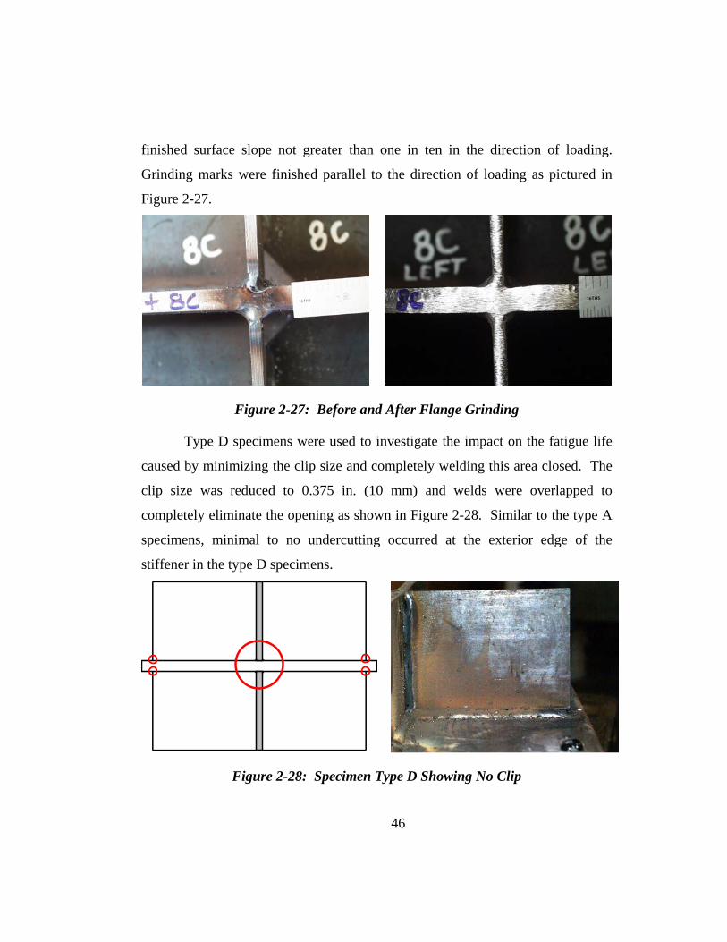
finished surface slope not greater than one in ten in the direction of loading.

Grinding marks were finished parallel to the direction of loading as pictured in

Figure 2-27.

Figure 2-27: Before and After Flange Grinding

Type D specimens were used to investigate the impact on the fatigue life

caused by minimizing the clip size and completely welding this area closed. The

clip size was reduced to 0.375 in. (10 mm) and welds were overlapped to

completely eliminate the opening as shown in Figure 2-28. Similar to the type A

specimens, minimal to no undercutting occurred at the exterior edge of the

stiffener in the type D specimens.

Figure 2-28: Specimen Type D Showing No Clip

46

2.5 MEASURING OF UNDERCUTS

The sizes of the undercuts are presented in this section. Undercuts were

measured with calipers and the values are presented in this section. The undercuts

were measured with calipers to an accuracy of +0.005 inches. The length, width,

and depth into the thickness of the stiffener were measured for the interior and

exterior stiffener undercuts. The length, width, and depth into the thickness of the

flange were measured for the flange undercuts.

2.5.1 Type A Specimen Undercuts

Undercut locations were labeled based on their orientation with respect to

their location in the test frame. Figure 2-29 shows the location and nomenclature

used for classification of type A specimen undercuts. The interior and exterior

stiffener undercuts were located on the top half (T) or bottom half (B) of the

specimen midsection.

front

back

T

T

B

B

Top Grip Bottom Grip

Strain Gages

2T 3T

6T 7T

1T

5T

4T

8T

Section T-T

3B 2B

7B 6B

4B

8B

1B

5B

Section B-B

Figure 2-29: Specimen A Undercut Identification 47

Table 2-1 lists the stiffener undercut dimensions corresponding to the

locations in Figure 2-29. Figure 3-30 illustrates the dimensions that were

recorded for the specimen A stiffener undercuts. Depth, d, refers to the depth into

the stiffener thickness. Measurements are given in inches.

Table 2-1: Specimen A Stiffener Undercut Measurements (inches)

UndercutI.D. L h d L h d L h d1T 0 0 0 0 0 0 0.050 0.050 0.0501B 0.350 0.350 0.035 0.180 0.320 0.120 0 0 02T 0.050 0.050 0.050 0.392 0.263 0.125 0 0 02B 0 0 0 0.102 0.100 0.125 0.075 0.050 0.0703T 0.244 0.100 0.125 0.316 0.092 0.125 0.075 0.050 0.0503B 0 0 0 0.113 0.145 0.125 0.050 0.050 0.0504T 0.090 0.150 0.113 0 0 0.0 0.075 0.075 0.0754B 0 0 0 0 0 0.0 0.075 0.075 0.0755T 0.035 0.079 0.065 0.050 0.050 0.050 0.075 0.100 0.0755B 0 0 0 0.075 0.075 0.075 0.050 0.050 0.0506T 0.080 0.085 0.080 0.050 0.050 0.050 0 0 06B 0.085 0.15 0.100 0.239 0.184 0.125 0 0 07T 0 0 0 0.162 0.086 0.125 0 0 07B 0 0 0 0.209 0.150 0.125 0 0 08T 0 0 0 0.050 0.050 0.050 0.100 0.100 0.1008B 0 0 0 0.050 0.050 0.050 0.100 0.100 0.100

Avg. 0.058 0.060 0.036 0.124 0.101 0.079 0.045 0.044 0.043Max. 0.350 0.350 0.125 0.392 0.320 0.125 0.100 0.100 0.100

1A 2A 3A

L

d h

INTERIOR

L

d h

EXTERIOR

Figure 2-30: Specimen A Stiffener Undercut Dimensions

48

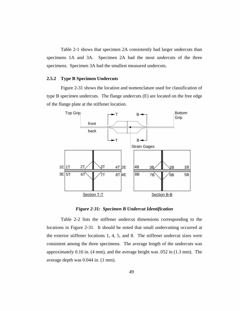
Table 2-1 shows that specimen 2A consistently had larger undercuts than

specimens 1A and 3A. Specimen 2A had the most undercuts of the three

specimens. Specimen 3A had the smallest measured undercuts.

2.5.2 Type B Specimen Undercuts

Figure 2-31 shows the location and nomenclature used for classification of

type B specimen undercuts. The flange undercuts (E) are located on the free edge

of the flange plate at the stiffener location.

2T 3T

6T 7T

1E

3E

2E

4E

Section T-T

1T

5T

4T

8T

3B 2B

7B 6B

Section B-B

4B

8B

1B

5B

front

back

T

T

B

B

Top Grip Bottom Grip

Strain Gages

Figure 2-31: Specimen B Undercut Identification

Table 2-2 lists the stiffener undercut dimensions corresponding to the

locations in Figure 2-31. It should be noted that small undercutting occurred at

the exterior stiffener locations 1, 4, 5, and 8. The stiffener undercut sizes were

consistent among the three specimens. The average length of the undercuts was

approximately 0.16 in. (4 mm), and the average height was .052 in (1.3 mm). The

average depth was 0.044 in. (1 mm).

49

Table 2-2: Specimen B Stiffener Undercut Measurements (inches)

UndercutI.D. L h d L h d L h d1T 0.050 0.050 0.050 0.050 0.100 0.050 0 0 01B 0.050 0.100 0.070 0.050 0.070 0.050 0 0 02T 0 0 0 0 0 0 0.050 0.050 0.0502B 0.050 0.050 0.050 0.186 0.125 0.125 0.050 0.050 0.0503T 0.050 0.050 0.050 0.200 0.065 0.125 0.050 0.050 0.0503B 0 0 0 0.050 0.050 0.050 0.115 0.050 0.1004T 0.064 0.085 0.050 0 0 0 0 0 04B 0.050 0.115 0.100 0.070 0.170 0.075 0.120 0.100 0.0705T 0.050 0.080 0.100 0 0 0 0.050 0.100 0.0505B 0.050 0.120 0.050 0 0 0 0.060 0.060 0.0506T 0.100 0.050 0.050 0.050 0.050 0.050 0.050 0.050 0.0506B 0 0 0 0.050 0.050 0.050 0.064 0.088 0.0907T 0 0 0 0.050 0.050 0.050 0 0 07B 0.135 0.105 0.070 0.360 0.110 0.050 0.0 0.0 08T 0.060 0.120 0.125 0.050 0.050 0.050 0.050 0.050 0.0508B 0 0 0 0 0 0 0 0 0

Avg. 0.044 0.058 0.048 0.073 0.056 0.045 0.041 0.041 0.038Max. 0.135 0.120 0.125 0.360 0.170 0.125 0.120 0.100 0.100

4B 5B 6B

Table 2-3 lists the flange undercut dimensions corresponding to the “E”

locations in Figure 2-31. Figure 3-33 illustrates the dimensions that were

measured for the specimen B flange undercuts. It should be noted that the flange

undercuts were considered more detrimental to the fatigue life of the specimen

than the exterior stiffener undercuts because of their direct orientation to loading.

Average measured values were consistent among all three specimens. The

average length of the flange undercuts was approximately 0.5 in. (13 mm), and

the average depth was over 0.125 in. (3 mm). The average width of the flange

undercuts was 0.072 in. (2 mm).

50

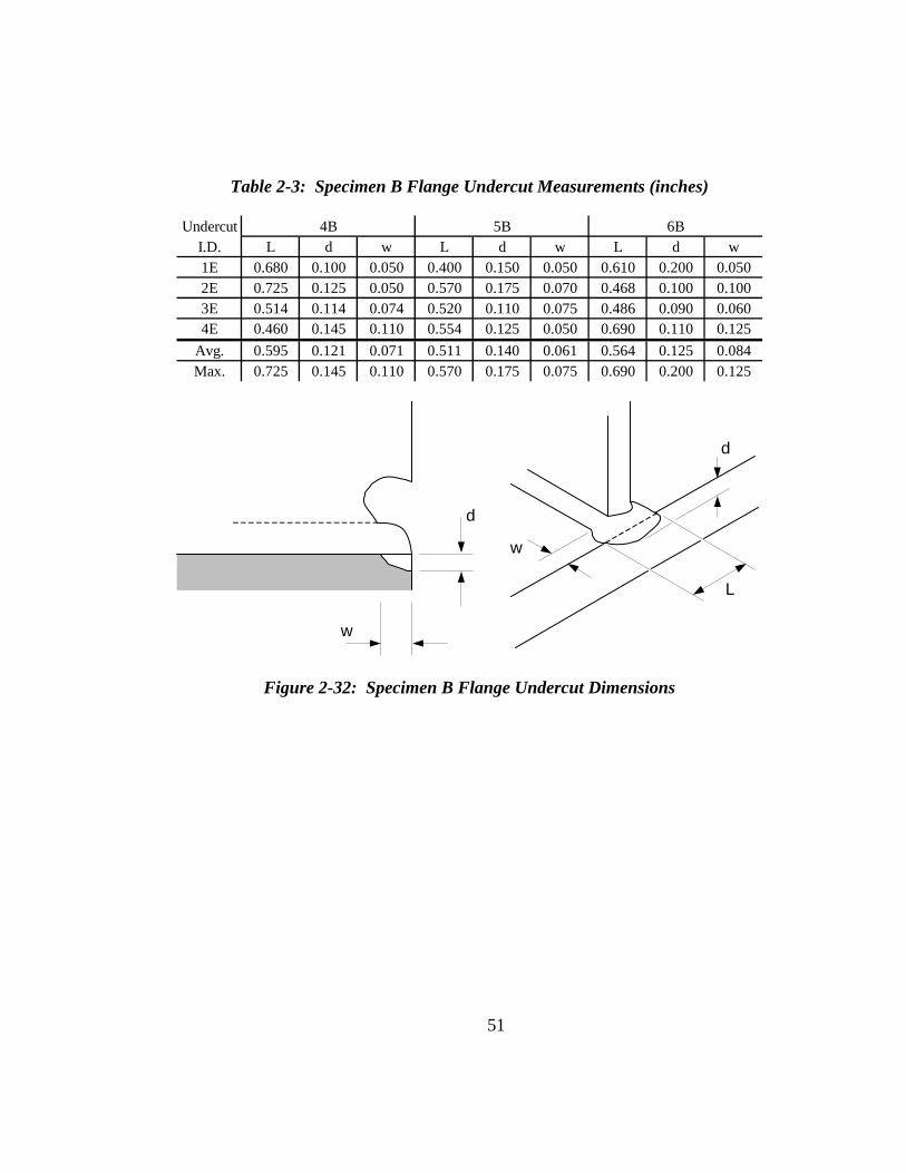
Table 2-3: Specimen B Flange Undercut Measurements (inches)

UndercutI.D. L d w L d w L d w1E 0.680 0.100 0.050 0.400 0.150 0.050 0.610 0.200 0.0502E 0.725 0.125 0.050 0.570 0.175 0.070 0.468 0.100 0.1003E 0.514 0.114 0.074 0.520 0.110 0.075 0.486 0.090 0.0604E 0.460 0.145 0.110 0.554 0.125 0.050 0.690 0.110 0.125

Avg. 0.595 0.121 0.071 0.511 0.140 0.061 0.564 0.125 0.084Max. 0.725 0.145 0.110 0.570 0.175 0.075 0.690 0.200 0.125

4B 5B 6B

d

L

w

d

w

Figure 2-32: Specimen B Flange Undercut Dimensions

51

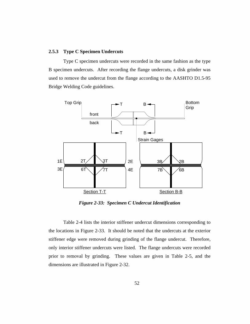
2.5.3 Type C Specimen Undercuts

Type C specimen undercuts were recorded in the same fashion as the type

B specimen undercuts. After recording the flange undercuts, a disk grinder was

used to remove the undercut from the flange according to the AASHTO D1.5-95

Bridge Welding Code guidelines.

3B 2B

7B 6B

Section B-B

2T 3T

6T 7T

1E

3E

2E

4E

Section T-T

front

back

T

T

B

B

Top Grip Bottom Grip

Strain Gages

Figure 2-33: Specimen C Undercut Identification

Table 2-4 lists the interior stiffener undercut dimensions corresponding to

the locations in Figure 2-33. It should be noted that the undercuts at the exterior

stiffener edge were removed during grinding of the flange undercut. Therefore,

only interior stiffener undercuts were listed. The flange undercuts were recorded

prior to removal by grinding. These values are given in Table 2-5, and the

dimensions are illustrated in Figure 2-32.

52

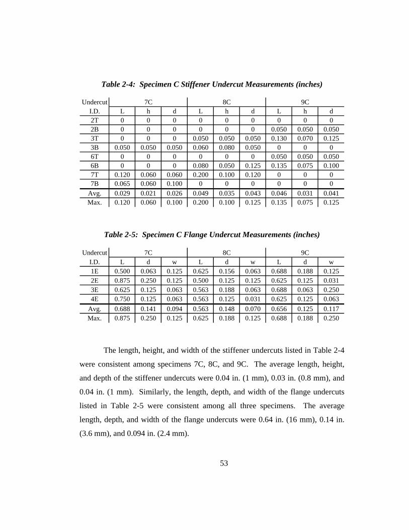
Table 2-4: Specimen C Stiffener Undercut Measurements (inches)

UndercutI.D. L h d L h d L h d2T 0 0 0 0 0 0 0 0 02B 0 0 0 0 0 0 0.050 0.050 0.0503T 0 0 0 0.050 0.050 0.050 0.130 0.070 0.1253B 0.050 0.050 0.050 0.060 0.080 0.050 0 0 06T 0 0 0 0 0 0 0.050 0.050 0.0506B 0 0 0 0.080 0.050 0.125 0.135 0.075 0.1007T 0.120 0.060 0.060 0.200 0.100 0.120 0 0 07B 0.065 0.060 0.100 0 0 0 0 0 0

Avg. 0.029 0.021 0.026 0.049 0.035 0.043 0.046 0.031 0.041Max. 0.120 0.060 0.100 0.200 0.100 0.125 0.135 0.075 0.125

7C 8C 9C

Table 2-5: Specimen C Flange Undercut Measurements (inches)

UndercutI.D. L d w L d w L d w1E 0.500 0.063 0.125 0.625 0.156 0.063 0.688 0.188 0.1252E 0.875 0.250 0.125 0.500 0.125 0.125 0.625 0.125 0.0313E 0.625 0.125 0.063 0.563 0.188 0.063 0.688 0.063 0.2504E 0.750 0.125 0.063 0.563 0.125 0.031 0.625 0.125 0.063

Avg. 0.688 0.141 0.094 0.563 0.148 0.070 0.656 0.125 0.117Max. 0.875 0.250 0.125 0.625 0.188 0.125 0.688 0.188 0.250

7C 8C 9C

The length, height, and width of the stiffener undercuts listed in Table 2-4

were consistent among specimens 7C, 8C, and 9C. The average length, height,

and depth of the stiffener undercuts were 0.04 in. (1 mm), 0.03 in. (0.8 mm), and

0.04 in. (1 mm). Similarly, the length, depth, and width of the flange undercuts

listed in Table 2-5 were consistent among all three specimens. The average

length, depth, and width of the flange undercuts were 0.64 in. (16 mm), 0.14 in.

(3.6 mm), and 0.094 in. (2.4 mm).

53

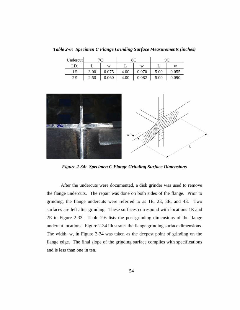
Table 2-6: Specimen C Flange Grinding Surface Measurements (inches)

UndercutI.D. L w L w L w1E 3.00 0.075 4.00 0.070 5.00 0.0552E 2.50 0.060 4.00 0.082 5.00 0.090

7C 8C 9C

54

w

L

Figure 2-34: Specimen C Flange Grinding Surface Dimensions

After the undercuts were documented, a disk grinder was used to remove

the flange undercuts. The repair was done on both sides of the flange. Prior to

grinding, the flange undercuts were referred to as 1E, 2E, 3E, and 4E. Two

surfaces are left after grinding. These surfaces correspond with locations 1E and

2E in Figure 2-33. Table 2-6 lists the post-grinding dimensions of the flange

undercut locations. Figure 2-34 illustrates the flange grinding surface dimensions.

The width, w, in Figure 2-34 was taken as the deepest point of grinding on the

flange edge. The final slope of the grinding surface complies with specifications

and is less than one in ten.

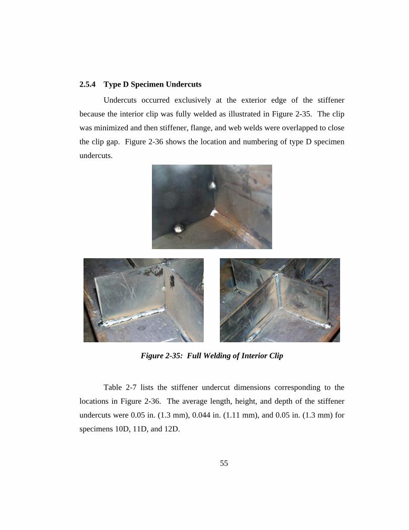
2.5.4 Type D Specimen Undercuts

Undercuts occurred exclusively at the exterior edge of the stiffener

because the interior clip was fully welded as illustrated in Figure 2-35. The clip

was minimized and then stiffener, flange, and web welds were overlapped to close

the clip gap. Figure 2-36 shows the location and numbering of type D specimen

undercuts.

Figure 2-35: Full Welding of Interior Clip

Table 2-7 lists the stiffener undercut dimensions corresponding to the

locations in Figure 2-36. The average length, height, and depth of the stiffener

undercuts were 0.05 in. (1.3 mm), 0.044 in. (1.11 mm), and 0.05 in. (1.3 mm) for

specimens 10D, 11D, and 12D.

55

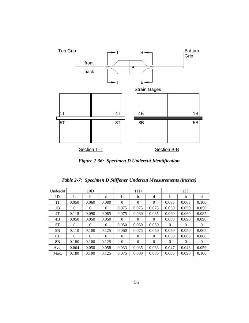
1T

5T

4T

8T

Section T-T

4B

8B

1B

5B

Section B-B

front

back

T

T

B

B

Top Grip Bottom Grip

Strain Gages

Figure 2-36: Specimen D Undercut Identification

Table 2-7: Specimen D Stiffener Undercut Measurements (inches)

UndercutI.D. L h d L h d L h d1T 0.050 0.060 0.080 0 0 0 0.085 0.065 0.1001B 0 0 0 0.075 0.075 0.075 0.050 0.050 0.0504T 0.118 0.090 0.085 0.075 0.080 0.085 0.060 0.060 0.0854B 0.050 0.050 0.050 0 0 0 0.080 0.090 0.0905T 0 0 0 0.050 0.050 0.050 0 0 05B 0.110 0.100 0.125 0.060 0.075 0.050 0.050 0.050 0.0658T 0 0 0 0 0 0 0.050 0.065 0.088B 0.180 0.100 0.125 0 0 0 0 0 0

Avg. 0.064 0.050 0.058 0.033 0.035 0.033 0.047 0.048 0.059Max. 0.180 0.100 0.125 0.075 0.080 0.085 0.085 0.090 0.100

10D 11D 12D

0

56

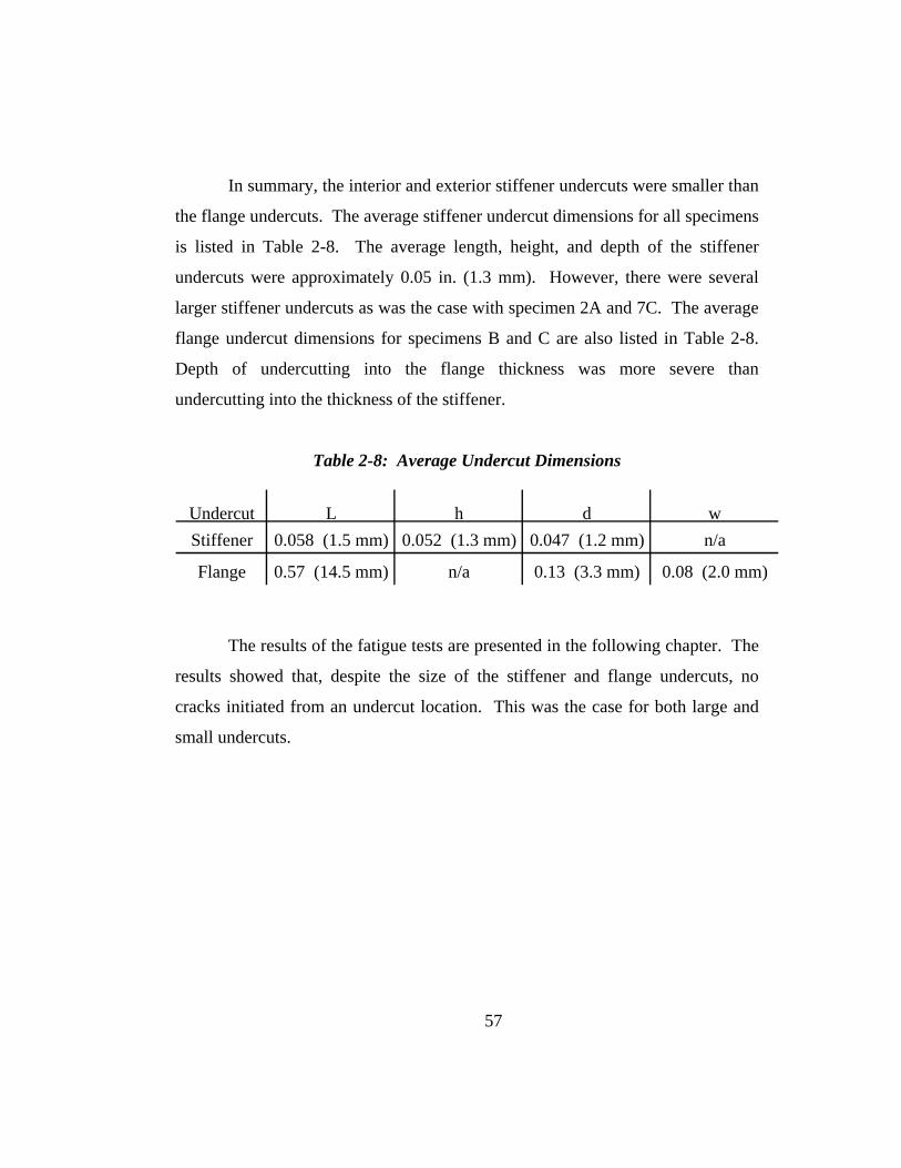
In summary, the interior and exterior stiffener undercuts were smaller than

the flange undercuts. The average stiffener undercut dimensions for all specimens

is listed in Table 2-8. The average length, height, and depth of the stiffener

undercuts were approximately 0.05 in. (1.3 mm). However, there were several

larger stiffener undercuts as was the case with specimen 2A and 7C. The average

flange undercut dimensions for specimens B and C are also listed in Table 2-8.

Depth of undercutting into the flange thickness was more severe than

undercutting into the thickness of the stiffener.

Table 2-8: Average Undercut Dimensions

Undercut L h d wStiffener 0.058 (1.5 mm) 0.052 (1.3 mm) 0.047 (1.2 mm) n/a

Flange 0.57 (14.5 mm) n/a 0.13 (3.3 mm) 0.08 (2.0 mm)

The results of the fatigue tests are presented in the following chapter. The

results showed that, despite the size of the stiffener and flange undercuts, no

cracks initiated from an undercut location. This was the case for both large and

small undercuts.

57

58

CHAPTER 2 Specimen Design and Fabrication ....................................... 22

2.1 Introduction ............................................................................... 22

2.2 Specimen Design ....................................................................... 27

2.2.1 Finite Element Model ............................................................ 33

2.3 Specimen Fabrication ................................................................ 37

2.3.1 Materials and Welding Parameters ....................................... 37

2.3.2 Assembly ............................................................................... 38

2.4 Details of Weld Undercuts ........................................................ 42

2.5 Measuring of Undercuts ............................................................ 47

2.5.1 Type A Specimen Undercuts ................................................. 47

2.5.2 Type B Specimen Undercuts ................................................. 49

2.5.3 Type C Specimen Undercuts ................................................. 52

2.5.4 Type D Specimen Undercuts ................................................. 55

Table 2-1: Specimen A Stiffener Undercut Measurements (inches) .................... 48

Table 2-2: Specimen B Stiffener Undercut Measurements (inches) .................... 50

Table 2-3: Specimen B Flange Undercut Measurements (inches) ....................... 51

Table 2-4: Specimen C Stiffener Undercut Measurements (inches) .................... 53

Table 2-5: Specimen C Flange Undercut Measurements (inches) ....................... 53

Table 2-6: Specimen C Flange Grinding Surface Measurements (inches) .......... 54

Table 2-7: Specimen D Stiffener Undercut Measurements (inches) .................... 56

Table 2-8: Average Undercut Dimensions ........................................................... 57

Figure 2-1: Steel Girder and Stiffener Detail Under Flexural Loading ............... 22

Figure 2-2: Test Specimen Showing Components and Cyclic Loading .............. 23

Figure 2-3: Specimen Cross-Section Geometry and Undercut Locations ........... 23

Figure 2-4: Photo Showing Variety of Specimens ............................................... 24

59

Figure 2-5: Test Specimen Dimensions ............................................................... 26

Figure 2-6: Location of Fatigue Categories ......................................................... 27

Figure 2-7: AASHTO Nominal Fatigue Resistance Categories B & C’ .............. 28

Figure 2-8: Area Used For Calculating Nominal Stress ...................................... 28

Figure 2-9: Radial Transition Region Showing High Stress ................................ 29

Figure 2-10: Finite Element Principal Stress Results (ksi) .................................. 33

Figure 2-11: Principal Stress Along Flange Path ................................................. 35

Figure 2-12: Principal Stress Along Web Path .................................................... 35

Figure 2-13: Welding the Web to the Flange ....................................................... 37

Figure 2-14: Steel Parts Prior to Welding ............................................................ 38

Figure 2-15: Weld Start-Stop Repair ................................................................... 39

Figure 2-16: Welding Sequence for Specimens 1A, 2A, 3A, and 7C .................. 39

Figure 2-17: Welding Sequence for Specimens 4B- 6B, and 10D-12D .............. 40

Figure 2-18: Welding Sequence for Specimens 8C and 9C ................................. 41

Figure 2-19: Location of Undercut for Specimen Type A ................................... 42

Figure 2-20: Large Circular Interior Stiffener Undercuts .................................... 43

Figure 2-21: Minimum Interior Stiffener Undercuts ............................................ 43

Figure 2-22: Specimen A Stiffener Undercut ...................................................... 43

Figure 2-23: Location of Undercut for Specimen Type B ................................... 44

Figure 2-24: Specimen B Stiffener Undercut ....................................................... 44

Figure 2-25: Specimen B Flange Undercuts ........................................................ 45

Figure 2-26: Location of Undercut for Specimen Type C ................................... 45

Figure 2-27: Before and After Flange Grinding ................................................... 46

Figure 2-28: Specimen Type D Showing No Clip ............................................... 46

Figure 2-29: Specimen A Undercut Identification ............................................... 47

Figure 2-30: Specimen A Stiffener Undercut Dimensions .................................. 48

Figure 2-31: Specimen B Undercut Identification ............................................... 49

60

Figure 2-32: Specimen B Flange Undercut Dimensions ...................................... 51

Figure 2-33: Specimen C Undercut Identification ............................................... 52

Figure 2-34: Specimen C Flange Grinding Surface Dimensions ......................... 54

Figure 2-35: Full Welding of Interior Clip ........................................................... 55

Figure 2-36: Specimen D Undercut Identification ............................................... 56

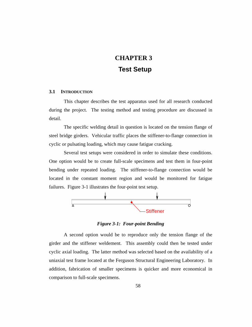
CHAPTER 3 Test Setup

3.1 INTRODUCTION

This chapter describes the test apparatus used for all research conducted

during the project. The testing method and testing procedure are discussed in

detail.

The specific welding detail in question is located on the tension flange of

steel bridge girders. Vehicular traffic places the stiffener-to-flange connection in

cyclic or pulsating loading, which may cause fatigue cracking.

Several test setups were considered in order to simulate these conditions.

One option would be to create full-scale specimens and test them in four-point

bending under repeated loading. The stiffener-to-flange connection would be

located in the constant moment region and would be monitored for fatigue

failures. Figure 3-1 illustrates the four-point test setup.

Stiffener

Figure 3-1: Four-point Bending

A second option would be to reproduce only the tension flange of the

girder and the stiffener weldement. This assembly could then be tested under

cyclic axial loading. The latter method was selected based on the availability of a

uniaxial test frame located at the Ferguson Structural Engineering Laboratory. In

addition, fabrication of smaller specimens is quicker and more economical in

comparison to full-scale specimens.

58

3.2 TEST APPARATUS

An MTS uniaxial hydraulic testing machine was employed to test the

specimens under cyclic loading. Pictured in Figure 3-2, the testing machine

consists of a load frame, actuator, and upper and lower grips. The hydraulic ram

is located below the lower grip and is out of view in Figure 3-2. A constant

pressure hydraulic pump provides the power for the system.

Figure 3-2: MTS Uniaxial Testing Machine with Specimen

59

3.2.1 Test Frame Components

Pictured in Figure 3-3, an MTS hydraulic actuator with a 220 kips (979

kN) capacity was used to apply the test load. The actuator has a total stroke of 6

in. (152 mm), which was controlled by either a remote POD or the computer via

the Testar II software. The actuator can be operated in either force or

displacement control. Force control was used for all the tests.

Figure 3-3: MTS Hydraulic Actuator

The test frame is equipped with custom upper and lower hydraulic grips

(model 641.385) that have a load rating of 220 kips (979 kN). The grips are

controlled using a hydraulic control module that regulates the gripping pressure.

The specimens were gripped using a pressure of approximately 2500 psi. (17.2

MPa). Figure 3-4 displays photographs of both the hydraulic grip and the

pressure control module.

60

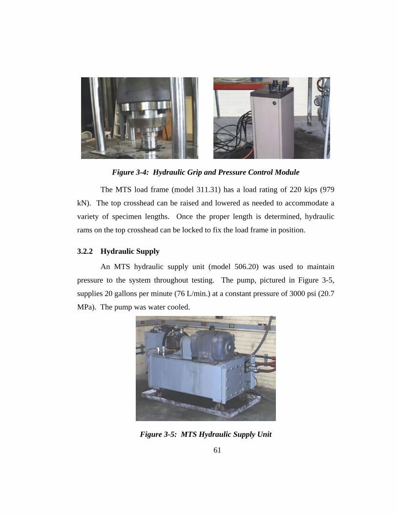
Figure 3-4: Hydraulic Grip and Pressure Control Module

The MTS load frame (model 311.31) has a load rating of 220 kips (979

kN). The top crosshead can be raised and lowered as needed to accommodate a

variety of specimen lengths. Once the proper length is determined, hydraulic

rams on the top crosshead can be locked to fix the load frame in position.

3.2.2 Hydraulic Supply

An MTS hydraulic supply unit (model 506.20) was used to maintain

pressure to the system throughout testing. The pump, pictured in Figure 3-5,

supplies 20 gallons per minute (76 L/min.) at a constant pressure of 3000 psi (20.7

MPa). The pump was water cooled.

Figure 3-5: MTS Hydraulic Supply Unit

61

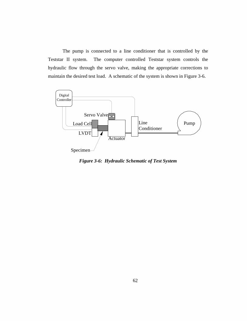
The pump is connected to a line conditioner that is controlled by the

Teststar II system. The computer controlled Teststar system controls the

hydraulic flow through the servo valve, making the appropriate corrections to

maintain the desired test load. A schematic of the system is shown in Figure 3-6.

Pump

Line Conditioner

Servo Valve

Actuator

Load Cell

LVDT

Specimen

Digital Controller

Figure 3-6: Hydraulic Schematic of Test System

62

3.3 TEST METHOD

All specimens were tested under cyclic axial tension with a minimum

stress greater than zero. Test parameters and the step-by-step test procedure are

discussed in this section.

3.3.1 Parameters

As previously discussed in Chapter 2.2, all specimens were tested under

cyclic loading at a nominal stress range, SR, of 20 ksi (138 MPa) and a stress

ratio, R, of 0.2. The stress ratio is defined as the minimum nominal stress divided

by the maximum nominal stress at the stiffener-to-flange connection. The

minimum and maximum nominal stresses across the connection detail were 5 ksi

(34.5 MPa) and 25 ksi (172 MPa), respectively.

tw

tf d

bf

( ) ( ffw bt dt 2 Area ⋅+⋅×= )

Figure 3-7: Area Used For Calculating Nominal Stress

The nominal stresses were calculated based on the area of the web plates

and the flange plate as shown in Figure 3-7. The area is located adjacent to the

63

stiffener detail. The lower stress limit corresponded to an axial load of 35 kips

(156 kN), whereas the upper stress limit was produced by an axial load of 175

kips (778 kN). Specimens were tested at either 1.50 Hz or 1.75 Hz. These

frequencies were used to avoid a rocking instability of the test frame. Tests

conducted at the reduced frequency of 1.50 Hz were done to limit the axial error

feedback to approximately 5 kips (22 kN). This axial error limit was considered

acceptable for all tests. The axial error occurred during transition from upper to

lower limits and did not affect the maximum and minimum loads. The maximum

and minimum loads were monitored and maintained throughout all testing. The

error at the 175 kip maximum loading was less than 0.3 kips, a difference of less

than 0.2% in applied load. The error at the 35 kip minimum loading was less than

0.2 kips, a difference of less than 0.6% in applied load. Figure 3-8 shows a graph

of the applied load versus time.

0

25

50

75

100

125

150

175

200

0 0.5 1 1.5 2 2.5 3

Time, t (sec.)

Load

, P (k

ips)

175 kips

35 kips

0.57 sec.

Figure 3-8: Experimental Applied Load versus Time

64

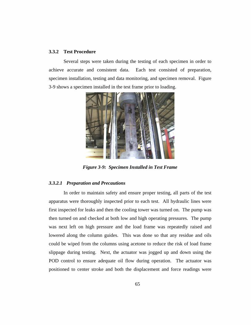
3.3.2 Test Procedure

Several steps were taken during the testing of each specimen in order to

achieve accurate and consistent data. Each test consisted of preparation,

specimen installation, testing and data monitoring, and specimen removal. Figure

3-9 shows a specimen installed in the test frame prior to loading.

Figure 3-9: Specimen Installed in Test Frame

3.3.2.1 Preparation and Precautions

In order to maintain safety and ensure proper testing, all parts of the test

apparatus were thoroughly inspected prior to each test. All hydraulic lines were

first inspected for leaks and then the cooling tower was turned on. The pump was

then turned on and checked at both low and high operating pressures. The pump

was next left on high pressure and the load frame was repeatedly raised and

lowered along the column guides. This was done so that any residue and oils

could be wiped from the columns using acetone to reduce the risk of load frame

slippage during testing. Next, the actuator was jogged up and down using the

POD control to ensure adequate oil flow during operation. The actuator was

positioned to center stroke and both the displacement and force readings were

65

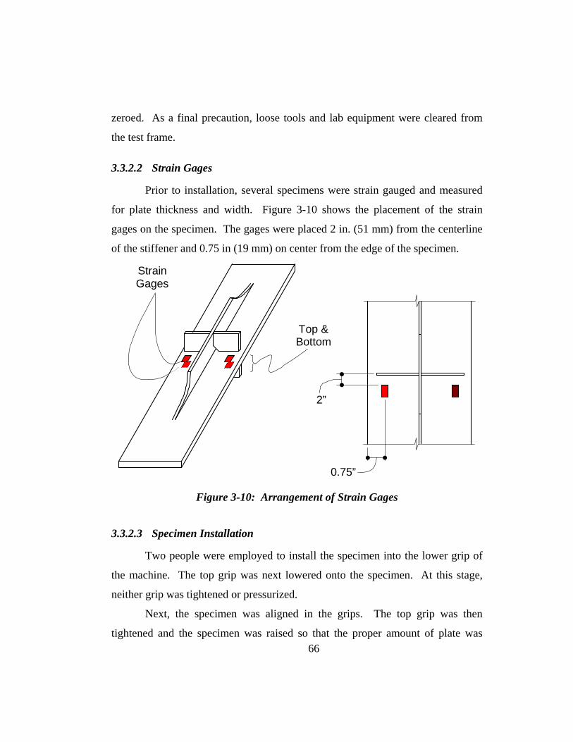
zeroed. As a final precaution, loose tools and lab equipment were cleared from

the test frame.

3.3.2.2 Strain Gages

Prior to installation, several specimens were strain gauged and measured

for plate thickness and width. Figure 3-10 shows the placement of the strain

gages on the specimen. The gages were placed 2 in. (51 mm) from the centerline

of the stiffener and 0.75 in (19 mm) on center from the edge of the specimen.

Strain Gages

Top & Bottom

2”

0.75”

Figure 3-10: Arrangement of Strain Gages

3.3.2.3 Specimen Installation

Two people were employed to install the specimen into the lower grip of

the machine. The top grip was next lowered onto the specimen. At this stage,

neither grip was tightened or pressurized.

Next, the specimen was aligned in the grips. The top grip was then

tightened and the specimen was raised so that the proper amount of plate was 66

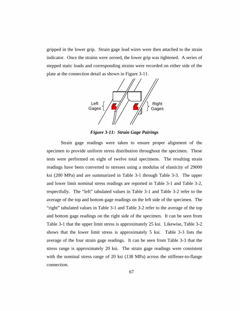
gripped in the lower grip. Strain gage lead wires were then attached to the strain

indicator. Once the strains were zeroed, the lower grip was tightened. A series of

stepped static loads and corresponding strains were recorded on either side of the

plate at the connection detail as shown in Figure 3-11.

Left Gages

Right Gages

Figure 3-11: Strain Gage Pairings

Strain gage readings were taken to ensure proper alignment of the

specimen to provide uniform stress distribution throughout the specimen. These

tests were performed on eight of twelve total specimens. The resulting strain

readings have been converted to stresses using a modulus of elasticity of 29000

ksi (200 MPa) and are summarized in Table 3-1 through Table 3-3. The upper

and lower limit nominal stress readings are reported in Table 3-1 and Table 3-2,

respectfully. The “left” tabulated values in Table 3-1 and Table 3-2 refer to the

average of the top and bottom gage readings on the left side of the specimen. The

“right” tabulated values in Table 3-1 and Table 3-2 refer to the average of the top

and bottom gage readings on the right side of the specimen. It can be seen from

Table 3-1 that the upper limit stress is approximately 25 ksi. Likewise, Table 3-2

shows that the lower limit stress is approximately 5 ksi. Table 3-3 lists the

average of the four strain gage readings. It can be seen from Table 3-3 that the

stress range is approximately 20 ksi. The strain gage readings were consistent

with the nominal stress range of 20 ksi (138 MPa) across the stiffener-to-flange

connection. 67

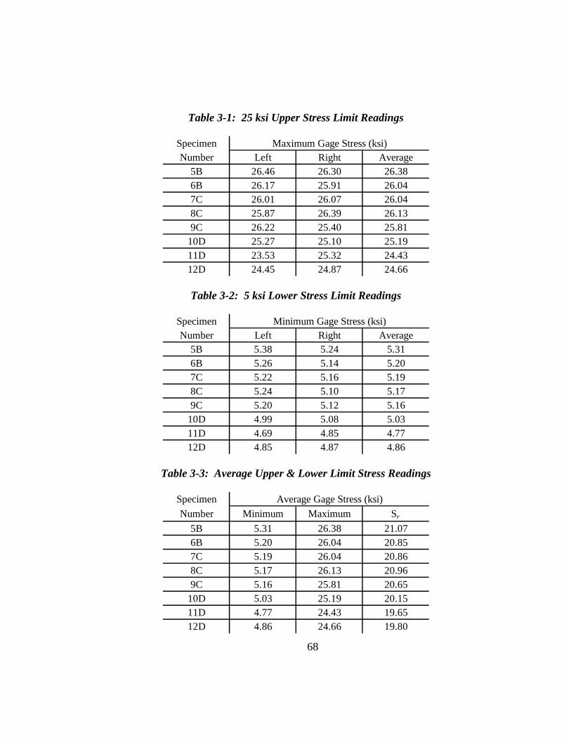
Table 3-1: 25 ksi Upper Stress Limit Readings

SpecimenNumber Left Right Average

5B 26.46 26.30 26.386B 26.17 25.91 26.047C 26.01 26.07 26.048C 25.87 26.39 26.139C 26.22 25.40 25.81

10D 25.27 25.10 25.1911D 23.53 25.32 24.4312D 24.45 24.87 24.66

Maximum Gage Stress (ksi)

Table 3-2: 5 ksi Lower Stress Limit Readings

SpecimenNumber Left Right Average

5B 5.38 5.24 5.316B 5.26 5.14 5.207C 5.22 5.16 5.198C 5.24 5.10 5.179C 5.20 5.12 5.16

10D 4.99 5.08 5.0311D 4.69 4.85 4.7712D 4.85 4.87 4.86

Minimum Gage Stress (ksi)

Table 3-3: Average Upper & Lower Limit Stress Readings

SpecimenNumber Minimum Maximum Sr

5B 5.31 26.38 21.076B 5.20 26.04 20.857C 5.19 26.04 20.868C 5.17 26.13 20.969C 5.16 25.81 20.65

10D 5.03 25.19 20.1511D 4.77 24.43 19.6512D 4.86 24.66 19.80

Average Gage Stress (ksi)

68

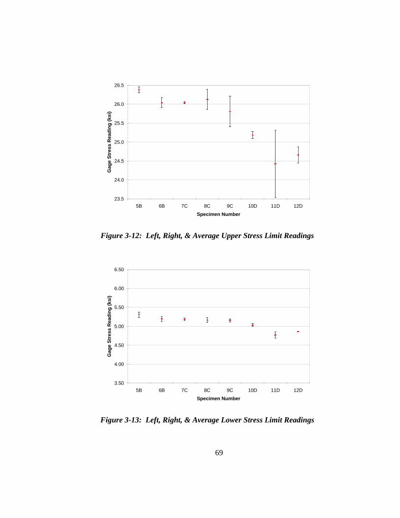
23.5

24.0

24.5

25.0

25.5

26.0

26.5

5B 6B 7C 8C 9C 10D 11D 12D

Specimen Number

Gag

e St

ress

Rea

ding

(ksi

)

Figure 3-12: Left, Right, & Average Upper Stress Limit Readings

3.50

4.00

4.50

5.00

5.50

6.00

6.50

5B 6B 7C 8C 9C 10D 11D 12D

Specimen Number

Gag

e St

ress

Rea

ding

(ksi

)

Figure 3-13: Left, Right, & Average Lower Stress Limit Readings

69

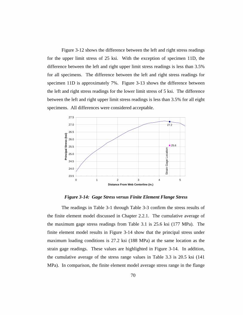
Figure 3-12 shows the difference between the left and right stress readings

for the upper limit stress of 25 ksi. With the exception of specimen 11D, the

difference between the left and right upper limit stress readings is less than 3.5%

for all specimens. The difference between the left and right stress readings for

specimen 11D is approximately 7%. Figure 3-13 shows the difference between

the left and right stress readings for the lower limit stress of 5 ksi. The difference

between the left and right upper limit stress readings is less than 3.5% for all eight

specimens. All differences were considered acceptable.

25.6

27.2

23.5

24.0

24.5

25.0

25.5

26.0

26.5

27.0

27.5

0 1 2 3 4 5

Distance From Web Centerline (in.)

Prin

cipa

l Str

ess

(ksi

)

Stra

in G

age

Loca

tion

Figure 3-14: Gage Stress versus Finite Element Flange Stress

The readings in Table 3-1 through Table 3-3 confirm the stress results of

the finite element model discussed in Chapter 2.2.1. The cumulative average of

the maximum gage stress readings from Table 3.1 is 25.6 ksi (177 MPa). The

finite element model results in Figure 3-14 show that the principal stress under

maximum loading conditions is 27.2 ksi (188 MPa) at the same location as the

strain gage readings. These values are highlighted in Figure 3-14. In addition,

the cumulative average of the stress range values in Table 3.3 is 20.5 ksi (141

MPa). In comparison, the finite element model average stress range in the flange

70

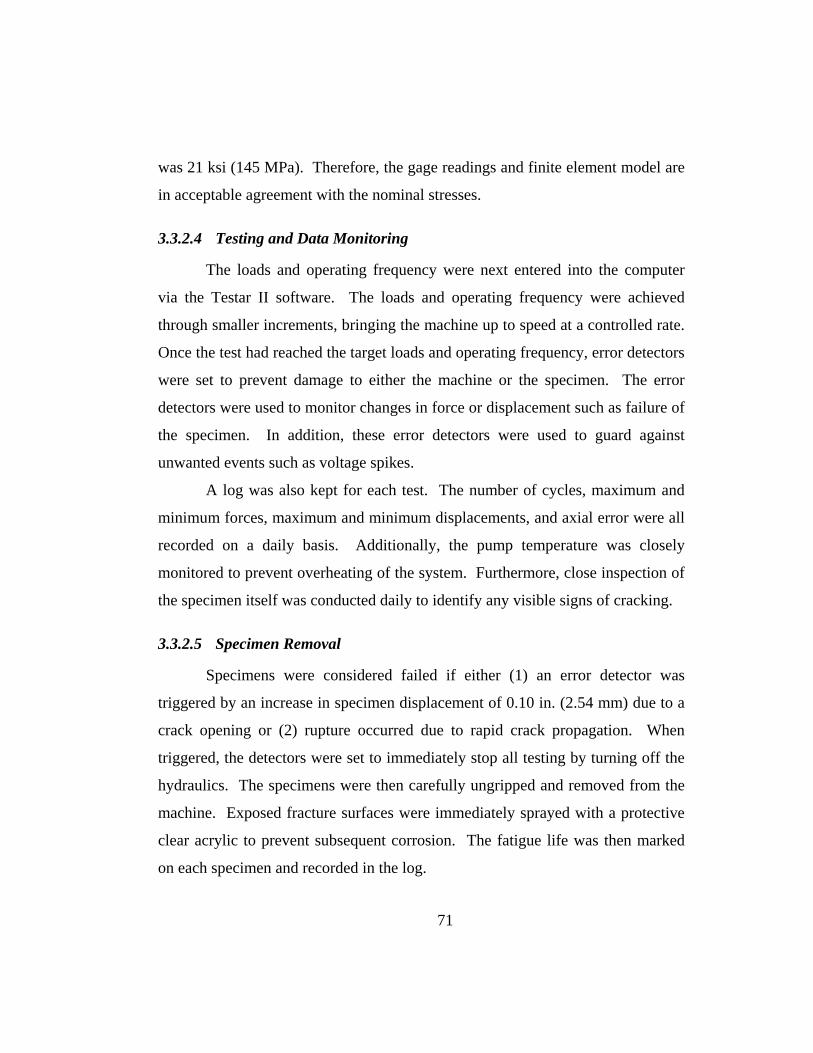
71

was 21 ksi (145 MPa). Therefore, the gage readings and finite element model are

in acceptable agreement with the nominal stresses.

3.3.2.4 Testing and Data Monitoring

The loads and operating frequency were next entered into the computer

via the Testar II software. The loads and operating frequency were achieved

through smaller increments, bringing the machine up to speed at a controlled rate.

Once the test had reached the target loads and operating frequency, error detectors

were set to prevent damage to either the machine or the specimen. The error

detectors were used to monitor changes in force or displacement such as failure of

the specimen. In addition, these error detectors were used to guard against

unwanted events such as voltage spikes.

A log was also kept for each test. The number of cycles, maximum and

minimum forces, maximum and minimum displacements, and axial error were all

recorded on a daily basis. Additionally, the pump temperature was closely

monitored to prevent overheating of the system. Furthermore, close inspection of

the specimen itself was conducted daily to identify any visible signs of cracking.

3.3.2.5 Specimen Removal

Specimens were considered failed if either (1) an error detector was

triggered by an increase in specimen displacement of 0.10 in. (2.54 mm) due to a

crack opening or (2) rupture occurred due to rapid crack propagation. When

triggered, the detectors were set to immediately stop all testing by turning off the

hydraulics. The specimens were then carefully ungripped and removed from the

machine. Exposed fracture surfaces were immediately sprayed with a protective

clear acrylic to prevent subsequent corrosion. The fatigue life was then marked

on each specimen and recorded in the log.

72

CHAPTER 3 Test Setup ............................................................................ 58

3.1 Introduction ............................................................................... 58

3.2 Test Apparatus ........................................................................... 59

3.2.1 Test Frame Components ........................................................ 60

3.2.2 Hydraulic Supply ................................................................... 61

3.3 Test Method ............................................................................... 63

3.3.1 Parameters ............................................................................. 63

3.3.2 Test Procedure ....................................................................... 65

Table 3-1: 25 ksi Upper Stress Limit Readings ................................................... 68

Table 3-2: 5 ksi Lower Stress Limit Readings ..................................................... 68

Table 3-3: Average Upper & Lower Limit Stress Readings ................................ 68

Figure 3-1: Four-point Bending ........................................................................... 58

Figure 3-2: MTS Uniaxial Testing Machine with Specimen ............................... 59

Figure 3-3: MTS Hydraulic Actuator ................................................................... 60

Figure 3-4: Hydraulic Grip and Pressure Control Module ................................... 61

Figure 3-5: MTS Hydraulic Supply Unit ............................................................. 61

Figure 3-6: Hydraulic Schematic of Test System ................................................ 62

Figure 3-7: Area Used For Calculating Nominal Stress ...................................... 63

Figure 3-8: Experimental Applied Load versus Time .......................................... 64

Figure 3-9: Specimen Installed in Test Frame ..................................................... 65

Figure 3-10: Arrangement of Strain Gages .......................................................... 66

Figure 3-11: Strain Gage Pairings ........................................................................ 67

Figure 3-12: Left, Right, & Average Upper Stress Limit Readings .................... 69

Figure 3-13: Left, Right, & Average Lower Stress Limit Readings .................... 69

Figure 3-14: Gage Stress versus Finite Element Flange Stress ............................ 70

73

72

CHAPTER 4 Fatigue Test Results

4.1 INTRODUCTION

The results of the fatigue tests are discussed in this chapter. The fatigue

life, or number of loading cycles to failure, was recorded and is presented for each

specimen. All specimens were tested at a nominal stress range, SR, of 20 ksi (138

MPa). A post mortem analysis of the specimens and photographs of the fracture

surfaces are included. An analysis of variance was performed on the data to

detect the differences, if any, among the fatigue performances of the specimen

types.

The test results given in this chapter confirm that specimen failure was

independent of undercutting at both the stiffener and flange. Failure of the

specimens was found to occur along the stiffener-to-flange weld toe. The likely

failure path of the specimens is shown in Figure 4-1. Figure 4-1 shows that the

fatigue cracks initiated at the stiffener-to-flange weld toe and propagated into the

thickness of the flange. Secondary cracks may begin to form at other weld toe

locations, but failure ultimately occurs due to the reduction in area as the cracks

continue to propagate into the flange.

Four stages of cracking are shown in Figure 4-1. A close-up of stage 1

crack section is shown in Figure 4-2. Smaller cracks form at the weld toe and

eventually coalesce in stage 2 to form a larger, shallow fatigue crack as shown in

Figure 4-3. In stage 3, the crack continues to grow through the flange as shown in

Figure 4-4. The crack growth is quicker along the surface of the flange due to the

large stress concentration at the weld toe.

(1)

(2)

(3)

View of Cracked Sections View of Flange

(4)

73Figure 4-1: Failure Path by Stage Number

74

Crack grow e 4-5 shows the

double

th becomes more rapid in Stage 4. Figur

-edged crack expanding along the length of the weld toe. Eventually, the

remaining flange edge will tear and the fatigue crack will rapidly propagate across

the rest of the flange. Figure 4-6 shows the resulting single-edged crack

propagation leading to failure of the specimens.

Figure 4-3: Stage 2

Figure 4-2: Stage 1

Figure 4-5: Stage 4

Figure 4-4: Stage 3

“Shear lip” caused by yielding of remaining area

Figure 4-6: Failure

75

4.2 S ECIMEN RESULTS

able 4-1 summarizes the fatigue test results of the specimens. The

i g fe of h specimens and the corresponding average measured

stress range values discussed in Chapter 3.3.2.3 are shown in Table 4-1. The

average fatigue life of each specim

P

T

result n fatigue li t e

en type is also listed in the table.

Table 4-1: Summary of Fatigue Testing Results

Stress Range Cycles to Failure AveSpecimen

rage Cyclesto Failure

1A 20 508,1992A 20* 439,185 459,2713A 20* 430,4294B 20* 212,6625B 21.1 628,377 448,3396B 20.8 503,9787C 20.9 574,0978C 21.0 435,863 479,5449C 20.7 428,672

10D 20.2 559,10611D 19.7 492,794 422,97812D 19.8 217,035

20.5** 452,533

Clip Opening Short stiffener

Clip Opening Long stiffener

Clip Opening Long stiffener

repaired

No

SR (ksi) Nf*

Clip Opening Short stiffener

Average*not measured; nominal SR=20 ksi

**does not include nominal values 1A through 4B

Specimen 5B had the longest fatigue life, failing at 628,377 cycles of

loading at a measured stress range of 21.1 ksi (145 MPa). Specimen 4B had the

shortest fatigue life, failing at 212,662 cycles. A nominal stress range of 20 ksi

was assum

ed for specimen 4B since the first four specimens were not strain

gauged. The average fatigue life of all specimens tested was 452,533 cycles. The

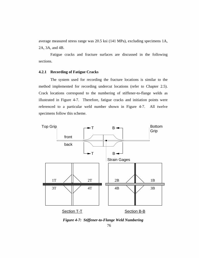
76

racks and fracture surfaces are discussed in the following

section

4.2.1 Recording of Fatigue Cracks

the fracture locations is similar to the

method

average measured stress range was 20.5 ksi (141 MPa), excluding specimens 1A,

2A, 3A, and 4B.

Fatigue c

s.

The system used for recording

implemented for recording undercut locations (refer to Chapter 2.5).

Crack locations correspond to the numbering of stiffener-to-flange welds as

illustrated in Figure 4-7. Therefore, fatigue cracks and initiation points were

referenced to a particular weld number shown in Figure 4-7. All twelve

specimens follow this scheme.

Section T-T

1T

3T

2T

4T

Section B-B

2B

4B

1B

3B

front

back

T

T

B

B

Top Grip Bottom Grip

Strain Gages

Figure 4-7: Stiffener-to-Flange Weld Numbering

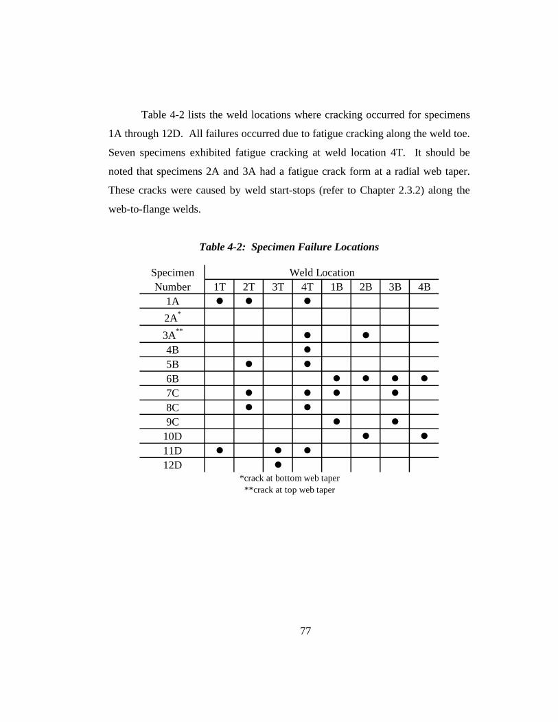
77

Table 4-2 lists the weld locations where cracking occurred for specimens

1A through 12D. All failures occurred due to fatigue cracking along the weld toe.

Seven specimens exhibited fatigue cracking at weld location 4T. It should be

noted that specimens 2A and 3A had a fatigue crack form at a radial web taper.

These cracks were caused by weld start-stops (refer to Chapter 2.3.2) along the

web-to-flange welds.

Table 4-2: Specimen Failure Locations

SpecimenNumber 1T 2T 3T 4T 1B 2B 3B 4B

1A2A*

3A**

4B5B6B

Weld Location

**crack at top web taper

7C8C9C

10D11D12D

*crack at bottom web taper

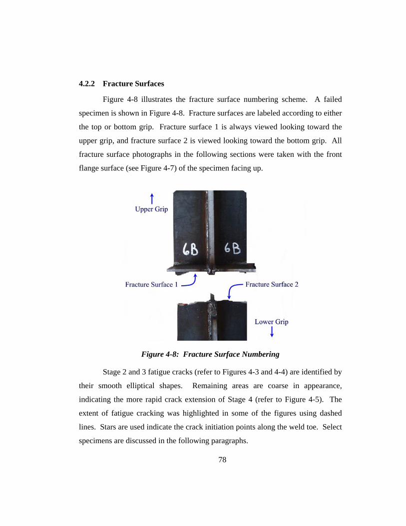
78

4.2.2 Fracture Su

Figure 4-8 illustrates the fracture surface numbering scheme. A failed

specimen is shown in Figure 4-8. Fracture surfaces are labeled according to either

the top or bottom grip. Fracture surface 1 is always viewed looking toward the

upper grip, and fracture surface 2 is viewed looking toward the bottom grip. All

fracture surface photographs in the following sections were taken with the front

flange surface (see Figure 4-7) of the specimen facing up.

rfaces

Figure 4-8: Fracture Surface Numbering

Stage 2 and 3 fatigue cracks (refer to Figures 4-3 and 4-4) are identified by

their smooth elliptical shapes. Remaining areas are coarse in appearance,

indicating the more rapid crack extension of Stage 4 (refer to Figure 4-5). The

extent of fatigue cracking was highlighted in some of the figures using dashed

lines. S ars are used indicate the crack initiation points along the weld toe. Select

specimens are discussed in the following paragraphs.

t

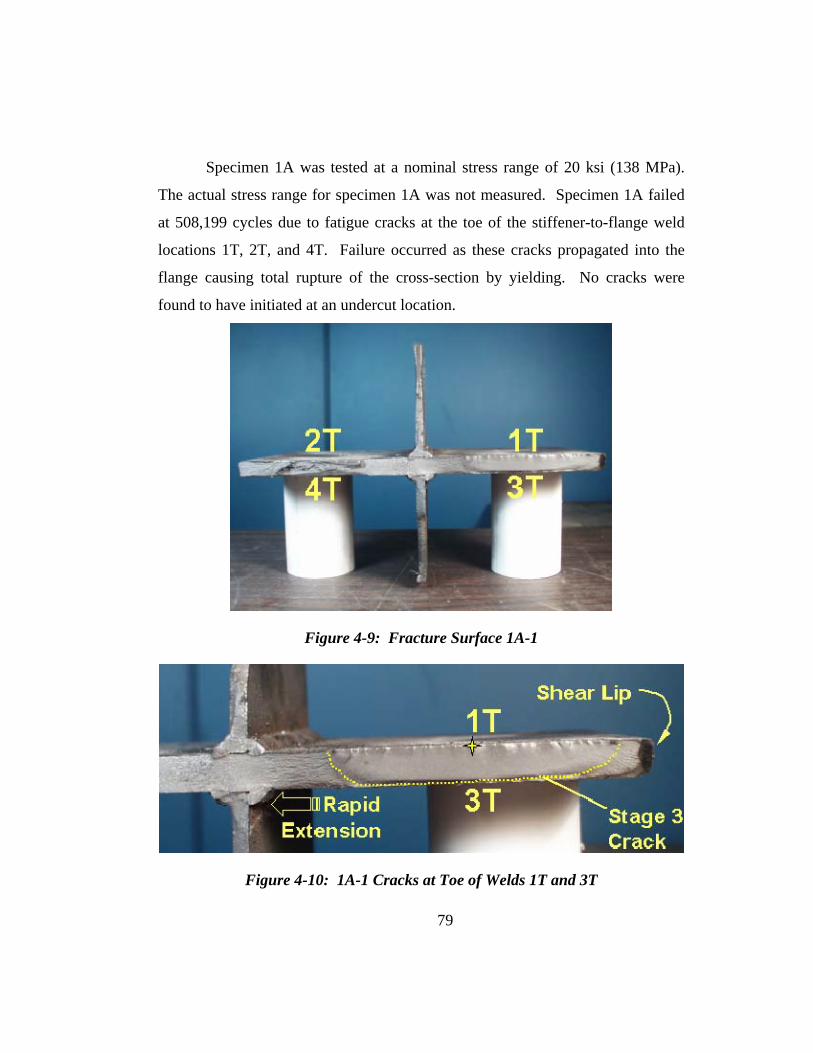
79

Specimen 1A was tested at a nominal stress range of 20 ksi (138 MPa).

The actual stress range for specimen 1A was not measured. Specimen 1A failed

at 508,199 cycles due to fatigue cracks at the toe of the stiffener-to-flange weld

locations 1T, 2T, and 4T. Failure occurred as these cracks propagated into the

flange causing total rupture of the cross-section by yielding. No cracks were

found to have initiated at an undercut location.

Figure 4-9: Fracture Surface 1A-1

Figure 4-10: 1A-1 Cracks at Toe of Welds 1T and 3T

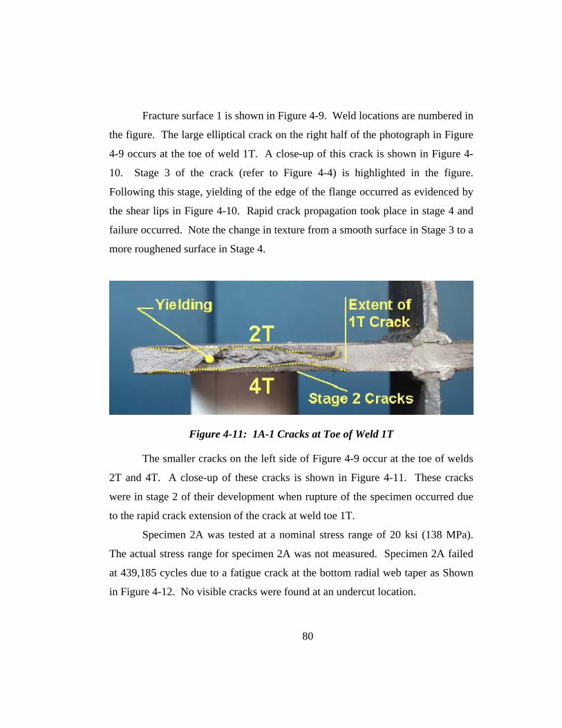
80

Fracture surface 1 is shown in Figure 4-9. Weld locations are numbered in

the figure. The large elliptical crack on the right half of the photograph in Figure

4-9 occurs at the toe of weld 1T. A close-up of this crack is shown in Figure 4-

10. Stage 3 of the crack (refer to Figure 4-4) is highlighted in the figure.

Following this stage, yielding of the edge of the flange occurred as evidenced by

the shear lips in Figure 4-10. Rapid crack propagation took place in stage 4 and

failure occurred. Note the change in texture from a smooth surface in Stage 3 to a

more roughened surface in Stage 4.

Figure 4-11: 1A-1 Cracks at Toe of Weld 1T

The smaller cracks on the left side of Figure 4-9 occur at the toe of welds

2T and 4T. A close-up of these cracks is shown in Figure 4-11. These cracks

were in stage ccurred due

to the r

2 of their development when rupture of the specimen o

apid crack extension of the crack at weld toe 1T.

Specimen 2A was tested at a nominal stress range of 20 ksi (138 MPa).

The actual stress range for specimen 2A was not measured. Specimen 2A failed

at 439,185 cycles due to a fatigue crack at the bottom radial web taper as Shown

in Figure 4-12. No visible cracks were found at an undercut location.

Figure 4-12: Fracture Surface 2A-1

The crack propagated into the flange from a weld start-stop. The start-

stop acted as an initial flaw in the web-to-flange weld and continued to grow

during testing. Figure 4-13 shows the initiation points at the weld start-stop. The

crack was believed to grow downward into the flange from these initiation points

causing a severe decrease in area resulting in rupture of the specimen.

Figure 4-13: 2A-2 Showing Flaws at Start-Stop 81

82

Specimen 3A was tested at a nominal stress range of 20 ksi (138 MPa).

The actual stress range for specimen 3A was not measured. Specimen 3A failed

at 430,429 cycles due to fatigue cracks at the toe of the stiffener-to-flange weld

locations 4T and 4B as shown in Figure 4-14. In addition, a third crack formed at

the upper radial web taper as shown in Figure 4-15. This crack formed due to a

weld stop-start in the web-to-flange weld (similar to specimen 2A). A specimen

displacement over the 0.10 in. limit halted the actuator prior to total rupture of the

specimen. No cracks were found to have initiated at an undercut location.

Figure 4-14: Multiple Cracks at Toe of Welds 4T and 4B

Figure 4-15: Crack at Upper Radial Web Taper

Failure at the radial tapers in specimens 2A and 3A led to revisions in the

welding sequence. A new welding sequence and repairs were employed to

eliminate failures at weld start-stop locations. Refer to Chapter 2.3.2 for details.

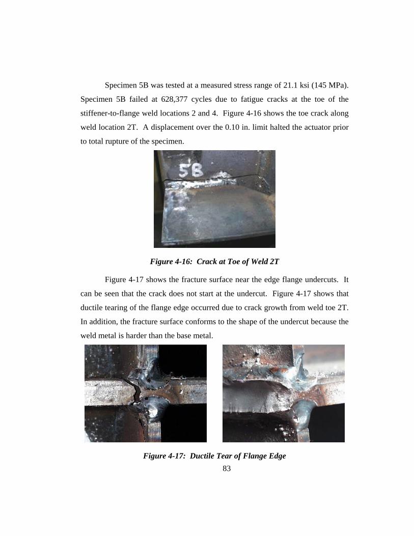
Specimen 5B was tested at a measured stress range of 21.1 ksi (145 MPa).

Specimen 5B failed at 628,377 cycles due to fatigue cracks at the toe of the

stiffener-to-flange weld locations 2 and 4. Figure 4-16 shows the toe crack along

weld location 2T. A displacement over the 0.10 in. limit halted the actuator prior

to total rupture of the specimen.

Figure 4-16: Crack at Toe of Weld 2T

Figure 4-17 shows the fracture surface near the edge flange undercuts. It

can be seen shows that

ductile tearing of the flange edge occurred due to crack growth from weld toe 2T.

In addition, the fracture surface conforms to the shape of the undercut because the

weld metal is harder than the base metal.

that the crack does not start at the undercut. Figure 4-17

Figure 4-17: Ductile Tear of Flange Edge 83

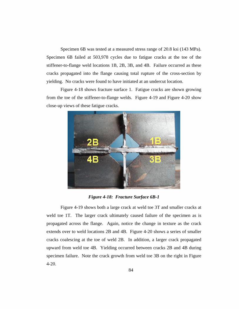
84

o have initiated at an undercut location.

Figure 4-18 shows fracture surface 1. Fatigue cracks are shown growing

from the toe of the stiffener-to-flange welds. Figure 4-19 and Figure 4-20 show

close-up views of these fatigue cracks.

Specimen 6B was tested at a measured stress range of 20.8 ksi (143 MPa).

Specimen 6B failed at 503,978 cycles due to fatigue cracks at the toe of the

stiffener-to-flange weld locations 1B, 2B, 3B, and 4B. Failure occurred as these

cracks propagated into the flange causing total rupture of the cross-section by

yielding. No cracks were found t

Figure 4-18: Fracture Surface 6B-1

Figure 4-19 shows both a large crack at weld toe 3T and smaller cracks at

weld toe 1T. The larger crack ultimately caused failure of the specimen as is

propagated across the flange. Again, notice the change in texture as the crack

extends over to weld locations 2B and 4B. Figure 4-20 shows a series of smaller

cracks coalescing at the toe of weld 2B. In addition, a larger crack propagated

upward from weld toe 4B. Yielding occurred between cracks 2B and 4B during

specimen failure. Note the crack growth from weld toe 3B on the right in Figure

4-20.

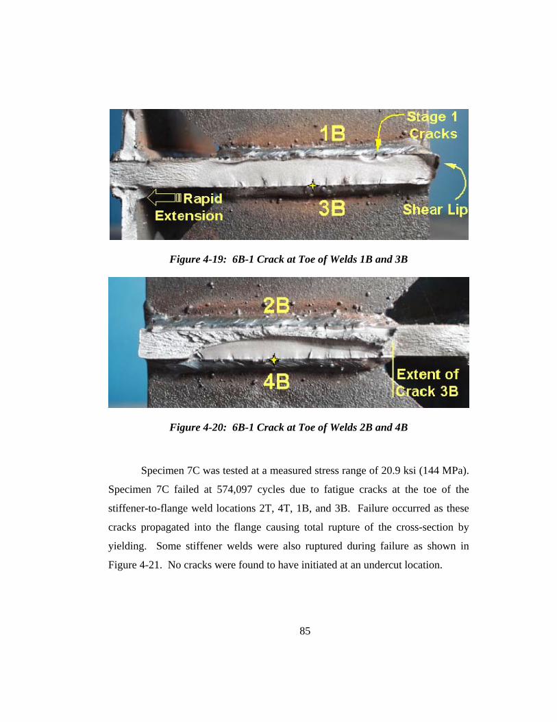
Figure 4-19: 6B-1 Crack at Toe of Welds 1B and 3B

Figure 4-20: 6B-1 Crack at Toe of Welds 2B and 4B

Specimen 7C was tested at a measured stress range of 20.9 ksi (144 MPa).

Specimen 7C failed at 574,097 cycles due to fatigue cracks at the toe of the

stiffener-to-flange weld locations 2T, 4T, 1B, and 3B. Failure occurred as these

cracks propagated into the flange causing total rupture of the cross-section by

yielding. Some stiffener welds were also ruptured during failure as shown in

Figure 4-21. No cracks were found to have initiated at an undercut location.

85

Figure 4-21: Failure of Specimen 7C

Figure d 4T do not

share the same plane as welds 1B and 3B. Fatigue cracks in Figure 4-23

originated from the toe of the stiffener-to-flange weld toe at weld locations 2T

and 4T. Fatigue cracks in Figure 4-24 originated from the toe of the stiffener-to-

flange weld toe at weld locations 1B and 3B.

4-22 shows fracture surface 1. Note that welds 2T an

Figure 4-22: Fracture surface 7C-1

86

Figure 4-23: 7C-1 Crack at Toe of Welds 2T and 4T

Figure 4-24: 7C-1 Crack at Toe of Welds 1B and 3B

Specimen 8C was tested at a measured stress range of 21 ksi (145 MPa).

Specimen 8C failed at 435,863 cycles due to fatigue cracks at the toe of the

stiffener-to-flange weld locations 2T and 4T. Figure 4-25 shows the toe crack

along weld location 2T. A displacement over the 0.10 in. limit halted the actuator

prior to total rupture of the specimen. No cracks were found to have initiated at

an undercut location.

87

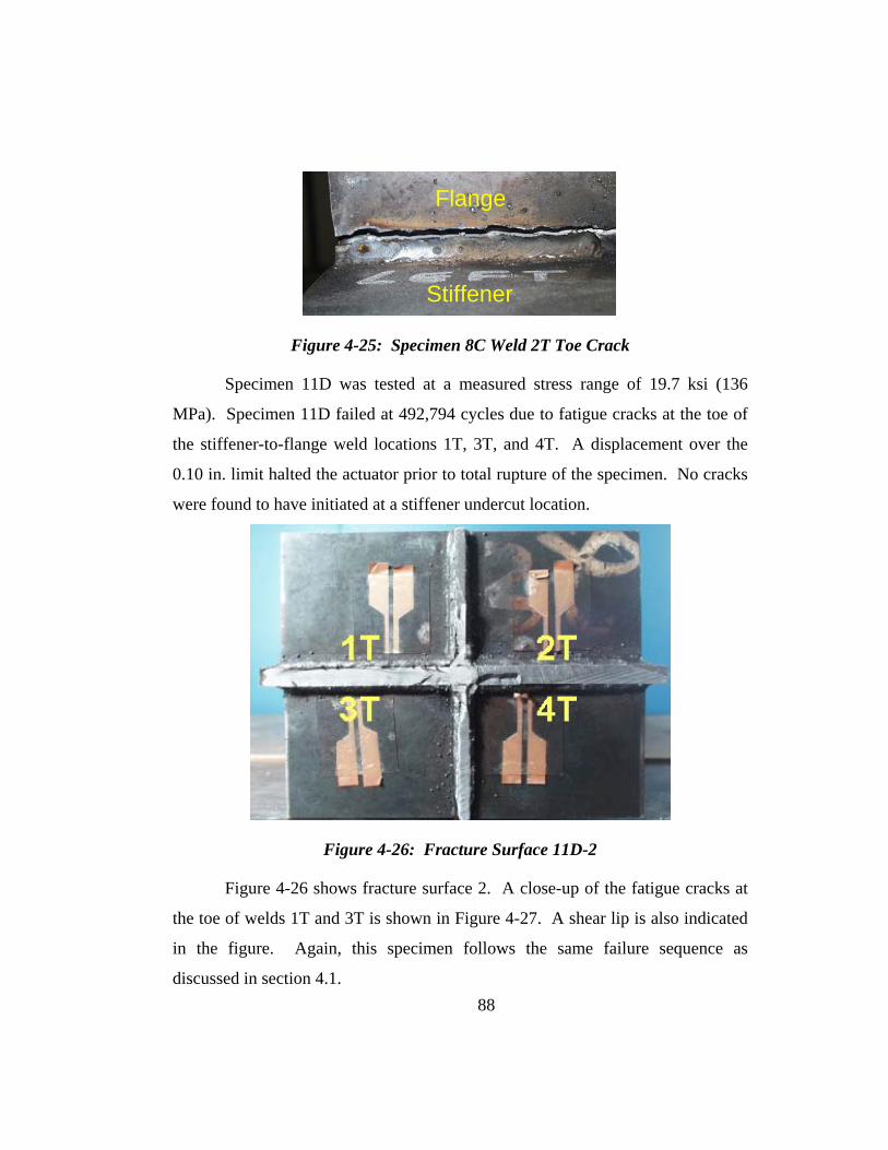
Stiffener

Flange

Stiffener

Flange

Figure 4-25: Specimen 8C Weld 2T Toe Crack

Specimen 11D was tested at a measured stress range of 19.7 ksi (136

MPa). Specim at the toe of

the stif ner-to-flange weld locations 1T, 3T, and 4T. A displacement over the

0.10 in. limit halted the actuator prior to total rupture of the specimen. No cracks

were found to have initiated at a stiffener undercut location.

en 11D failed at 492,794 cycles due to fatigue cracks

fe

Figure 4-26: Fracture Surface 11D-2

Figure 4-26 shows fracture surface 2. A close-up of the fatigue cracks at

the toe of welds 1T and 3T is shown in Figure 4-27. A shear lip is also indicated

in the figure. Again, this specimen follows the same failure sequence as

discussed in section 4.1. 88

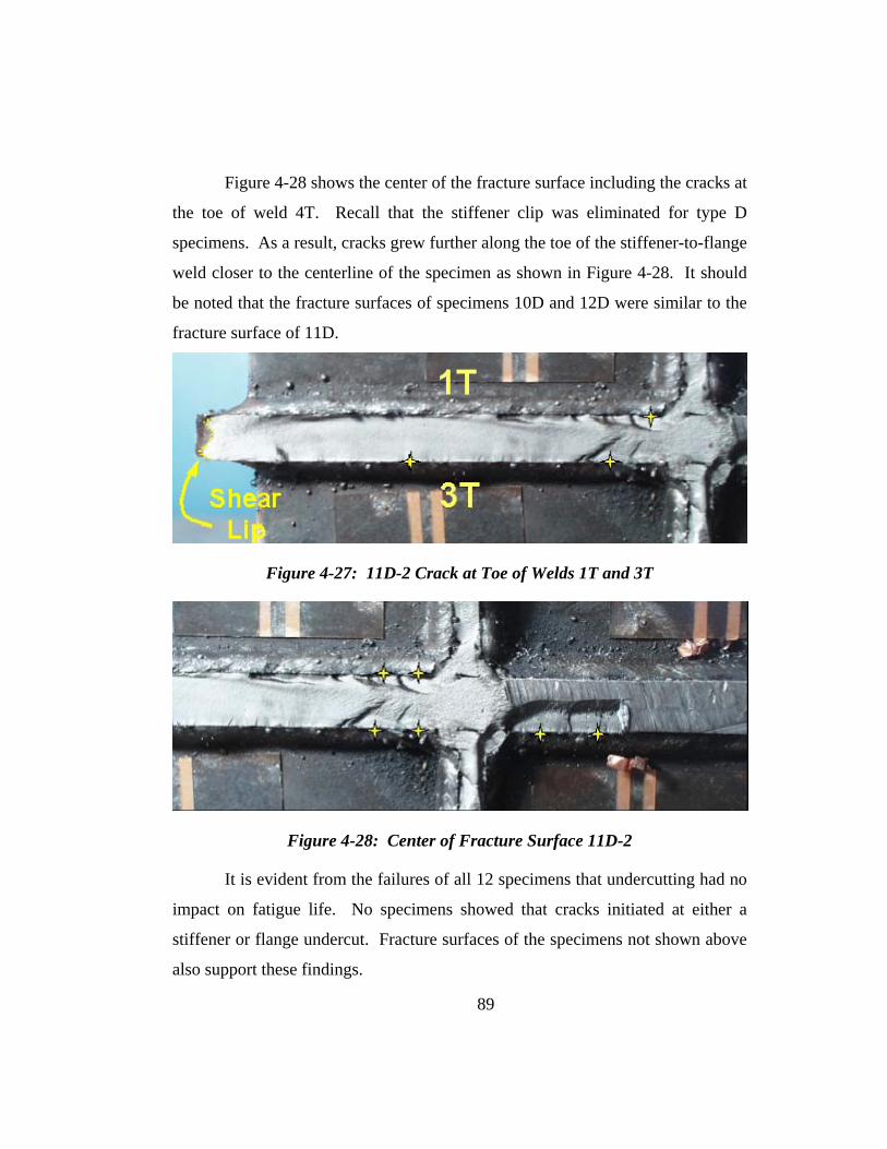
89

Figure 4-28 shows the center of the fracture surface including the cracks at

the toe of weld 4T. Recall that the stiffener clip was eliminated for type D

specimens. As a result, cracks grew further along the toe of the stiffener-to-flange

weld closer to the centerline of the specimen as shown in Figure 4-28. It should

be noted that the fracture surfaces of specimens 10D and 12D ere similar to the

fracture surface o

w

f 11D.

Figure 4-27: 11D-2 Crack at Toe of Welds 1T and 3T

Figure 4-28: Center of Fracture Surface 11D-2

s.

It is evident from the failures of all 12 specimens that undercutting had no

impact on fatigue life. No specimens showed that cracks initiated at either a

stiffener or flange undercut. Fracture surfaces of the specimens not shown above

also support these finding

90

4.3 D

1) compare the AASHTO category C’ nominal fatigue

resistance to the resulting fatigue life of the specimens; and (2) to determine if

there is a significant difference between the fatigue life of the type A, B, C, and D

specimens due to stiffener geometry and undercutting caused by fully sealing the

stiffener weld.

4.3.1 Comparison with AASHTO Fatigue Resistance

Figure 4-29 shows the results of the fatigue tests plotted along with the

category C’ life of the

specimens is 550,000 cycles at a stress range of 20 ksi (138 MPa). The average

fatigue life of all specimens tested was 452,533 cycles with an average measured

stress range of 20.5 ksi (141 MPa).

ATA ANALYSIS

The results of the fatigue tests are evaluated in this section. The fatigue

lives of the specimens were compared to the AASHTO nominal fatigue resistance

category C’ line. In addition, a single-factor analysis of variance (ANOVA) test

was performed on the specimen groups using Microsoft Excel. The purpose of

the data analyses is to (

nominal fatigue resistance line. The design fatigue

10

100St

ress

Ran

ge,

S R (

KSI

) Category C' Type A Type B Type C Type D

1.0E+05 1.0E+06

Cycles to Failure, Nf

icted life. The fatigue life is a function of

stress range in the following equation previously used in Chapter 2.2.

Figure 4-29: Comparison with Category C’ Fatigue Resistance

The recorded stress range was higher than the nominal stress range at the

stiffener connection. This may be one reason that average fatigue life of the

specimens was lower than the pred

( ) ( )-3RC

8C S1044 N ⋅×=

This is the equation of the C’-line shown in Figure 4-29. Table 4-3 lists

the stress range and fatigue life of the experimental values in comparison to the

AASHTO C’-line equation. Based on the minimum and maximum measured

stress range of 19.7 ksi (136 MPa) and 21.1 ksi (145 MPa), the AASHTO nominal

fatigue life ranges from 575,511 cycles to 468,388 cycles, respectively. At an

average measured stress range of 20.5 ksi (141 MPa), the average fatigue life of

specimens 1A through 12D was 452,533 cycles. This average is 15,855 cycles

91

92

lower than the minimum nominal fatigue life based on the AASHTO C’-line

equation using a stress range of 21.1 ksi (145 MPa).

Table 4-3: Comparison of Actual and Predicted Fatigue Life

Stress Range Cycles to FailureSR (ksi) Nf

Average Test Results 20.5 452,533

AASHTO Category C

19.7 21.1

575,511 468,388

CASE

Although the average fatigue life of the specimens is lower than the

AASHTO C’-line prediction, it is believed that failure of the specimens was due

to crack initiation at the stiffener-to-flange weld toe as established in section 4.2

of this chapter. The low

uniform stress in the flange plate and the larger stress concentration resulting from

the stif

ed on the

resulting fatigue lives of the type A, B, C, and D specimens. The analysis was

used to compare the mean fatigue life of each specimen type to determine if they

are sig

er life is most likely due to the slightly higher and non-

fener on both sides of the flange.

4.3.2 Analysis of Variance

A single factor analysis of variance (ANOVA) was perform

nificantly different or not significantly different. Findings from the

analysis of variance indicated that there is no significant difference between the

fatigue performance of the type A, B, C, and D specimens. The analysis was

based on the assumption that differences in the measured stress range for each test

specimen were irrelevant.

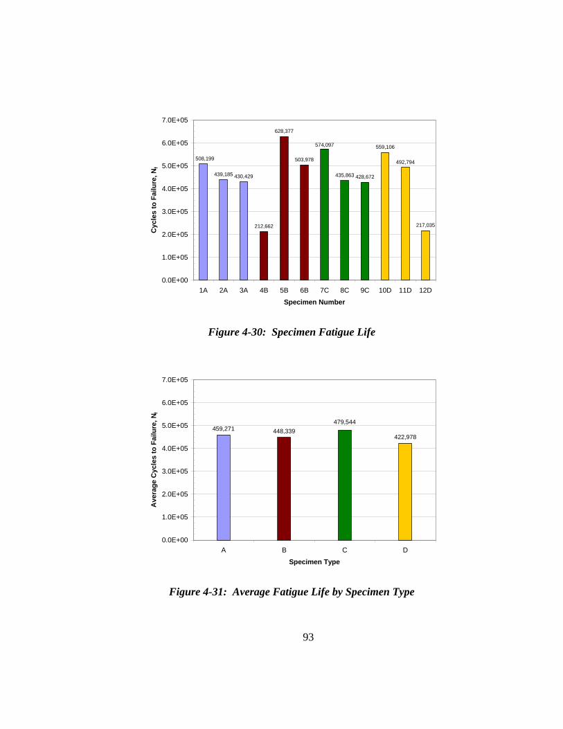
439,185 430,429

212,662

628,377

6.0E+05

7.0E+05

503,978

559,106

492,794508,199

574,097

435,863 428,672

217,035

1.0E+05

2.0E+05

3.0E+05

4.0E+05

5.0E+05

Cyc

les

to F

ailu

re, N

f

0.0E+001A 2A 3A 4B 5B 6B 7C 8C 9C 10D 11D 12D

Specimen Number

Figure 4-30: Specimen Fatigue Life

7.0E+05

459,271 448,339422,978

0.0E+00

1.0E+05

2.0E+05

3.0E+05

4.0E+05

5.0E+05

A B C D

Ave

rage

Cyc

les

to F

ailu

re, N 479,544

6.0E+05

Specimen Type

Figure 4-31: Average Fatigue Life by Specimen Type

f

93

94

Figure 4-30 shows a bar graph of the fatigue life of each specimen. The

average fatigue life of all twelve specimens was 452,533 cycles. Figure 4-31

shows a bar graph of the average fatigue life of each specimen type. The average

fatigue life of the type A, B, C, and D specimens was 459,271, 448,339, 479,544,

and 422,978 cycles, respectively. The analysis of variance compares the mean

life of each specimen type as well as the variance, or standard deviation, within

and between each specimen type.

Table 4-4: Average Fatigue Life and Standard Deviation by Specimen Type

Specimen Average Cycles StandardType to Failure Deviation

A 459,271 42,59869

C 479,544 81,964D 422,978 181,408

B 448,339 213,3

Table 4-4 summarizes the average fatigue life and standard deviation for

the type A, B, C, and D specimens. The type C specimens had the longest mean

fatigue life at 479,544 cycles. The Type D specimens had shortest mean fatigue

life at 422,978 cycles. The difference between these fatigue life means is less

than 12%. It can be seen from Figure 4-30 and Table 4-4 that the type A and type

C specimens exhibit the least variance. The large standard deviation of the type B

and D specimens is due to the short fatigue life of specimens 4B and 12D,

respectfully. However, it should be noted that a thirteenth specimen was actually

tested prior to specimen 12D. This additional type D specimen had lasted

292,583 cycles, more than the life of specimen 12D, prior to being inadvertently

crushed due to a system o visible

signs of cracking at the time of the accident. Specimen 12D was then fabricated

to replace the damaged specimen.

failure triggered by a severe storm. There were n

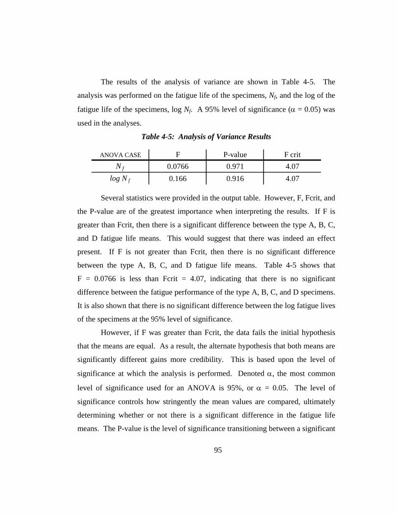
The results of the analysis of variance are shown in Table 4-5. The

analysis was performed on the fatigue life of the specimens, Nf, and the log of the

fatigue life of the specimens, log Nf. A 95% level of significance (α = 0.05) was

used in the analyses.

Table 4-5: Analysis of Variance Results

ANOVA CASE F P-value F critN f 0.0766 0.971 4.07

log N f 0.166 0.916 4.07

Several statistics were provided in the output table. However, F, Fcrit, and

the P-value are of the greatest importance when interpreting the results. If F is

greater than Fcrit, then there is a significant difference between the type A, B, C,

and D fatigue life means. This would suggest that there was indeed an effect

present. If F is not greater than Fcrit, then there is no significant difference

between the type A, B, C, and D fatigue life means. Table 4-5 shows that

F = 0.0766 is less than Fcrit = 4.07, indicating that there is no significant

difference between the fatigue performance of the type A, B, C, and D specimens.

It is also shown that there is no significant difference between the log fatigue lives

of the specimens at the 95% level of significance.

However, if F was greater than Fcrit, the data fails the initial hypothesis

that the means are equal. As a result, the alternate hypothesis that both means are

significantly different gains more credibility. This is based upon the level of

significance at which the analysis is performed. Denoted α, the most common

level of significance used for an ANOVA is 95%, or α = 0.05. The level of

significance controls how stringently the mean values are compared, ultimately

determining whether or not there is a significant difference in the fatigue life

means. The P-value is the level of significance transitioning between a significant

95

96

outcom

erformance of the type A, B, C, and D specimens. In this

case, using a level o ly illogical, further

supporting the hypothesis that there is no significant difference between the

fatigue performances of the various specimen types.

e as opposed to an insignificant outcome. The P-value given in Table 4-5

is 0.971. Therefore, a level of significance (α) equal to this P-value would be

needed to create an outcome indicating that there is a significant difference

between the fatigue p

f significance of α = 0.971 would be high

97

ue Resistance ................... 90

4.3.2 Analysis of Variance ............................................................. 92

Table 4-1: Summary of Fatigue Testing Results .................................................. 75

Table 4-2: Specimen Failure Locations ............................................................... 77

Table 4-3: Comparison of Actual and Predicted Fatigue Life ............................. 92

Table 4-4: Average Fatigue Life and Standard Deviation by Specimen Type .... 94

Table 4-5: Analysis of Variance Results .............................................................. 95

Figure 4-1: Failure Path by Stage Number ........................................................... 73

Figure 4-2: Stage 1 ............................................................................................... 74

Figure 4-3: Stage 2 ............................................................................................... 74

Figure 4-4: Stage 3 ............................................................................................... 74

Figure 4-5: Stage 4 ............................................................................................... 74

Figure 4-6: Failure ................................................................................................ 74

Figure 4-7: Stiffener-to-Flange Weld Numbering................................................ 76

Figure 4-8: Fracture Surface Numbering ............................................................. 78

Figure 4-9: Fracture Surface 1A-1 ....................................................................... 79

Figure 4-10: 1A-1 Cracks at Toe of Welds 1T and 3T ........................................ 79

Figure 4-11: 1A-1 Cracks at Toe of Weld 1T ...................................................... 80

Figure 4-12: Fracture Surface 2A-1 ..................................................................... 81

CHAPTER 4 Fatigue Test Results ............................................................ 72

4.1 Introduction ............................................................................... 72

4.2 Specimen Results ...................................................................... 75

4.2.1 Recording of Fatigue Cracks ................................................. 76

4.2.2 Fracture Surfaces ................................................................... 78

4.3 Data Analysis ............................................................................ 90

4.3.1 Comparison with AASHTO Fatig

98

Figure

Figure 4-

Figure 4-

Figure 4-16 k

Figure 4-17

Figure 4-

Figure 4-19

Figure 4-20

Figure 4-21: Failure of Specimen 7C ................................................................... 86

Figure 4-27: 11D-2 Crack at Toe of Welds 1T and 3T ........................................ 89

4-13: 2A-2 Showing Flaws at Start-Stop .................................................. 81

14: Multiple Cracks at Toe of Welds 4T and 4B ................................... 82

15: Crack at Upper Radial Web Taper .................................................. 82

: Crac at Toe of Weld 2T ................................................................. 83

: Ductile Tear of Flange Edge ........................................................... 83

18: Fracture Surface 6B-1 ..................................................................... 84

: 6B-1 Crack at Toe of Welds 1B and 3B .......................................... 85

: 6B-1 Crack at Toe of Welds 2B and 4B .......................................... 85

Figure 4-22: Fracture surface 7C-1 ...................................................................... 86

Figure 4-23: 7C-1 Crack at Toe of Welds 2T and 4T .......................................... 87

Figure 4-24: 7C-1 Crack at Toe of Welds 1B and 3B .......................................... 87

Figure 4-25: Specimen 8C Weld 2T Toe Crack ................................................... 88

Figure 4-26: Fracture Surface 11D-2 ................................................................... 88

Figure 4-28: Center of Fracture Surface 11D-2 ................................................... 89

Figure 4-29: Comparison with Category C’ Fatigue Resistance .......................... 91

Figure 4-30: Specimen Fatigue Life ..................................................................... 93

Figure 4-31: Average Fatigue Life by Specimen Type ........................................ 93

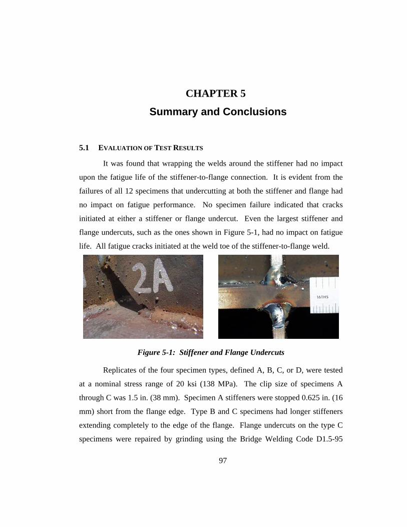
CHAPTER 5 Summary and Conclusions

5.1 EVALUATION OF TEST RESULTS

It was found that wrapping the welds around the stiffener had no impact

upon the fatigue life of the stiffener-to-flange connection. It is evident from the

failures of all 12 specimens that undercutting at both the stiffener and flange had

no impact on fatigue performance. No specimen failure indicated that cracks

initiated at either a stiffener or flange undercut. Even the largest stiffener and

flange undercuts, such as the ones shown in Figure 5-1, had no impact on fatigue

life. All fatigue cracks initiated at the weld toe of the stiffener-to-flange weld.

Figure 5-1: Stiffener and Flange Undercuts

Replicates of the four specimen types, defined A, B, C, or D, were tested

at a nominal stress range of 20 ksi (138 MPa). The clip size of specimens A

through C was 1.5 in. (38 mm). Specimen A stiffeners were stopped 0.625 in. (16

mm) short from the flange edge. Type B and C specimens had longer stiffeners

extending completely to the edge of the flange. Flange undercuts on the type C

specimens were repaired by grinding using the Bridge Welding Code D1.5-95

97

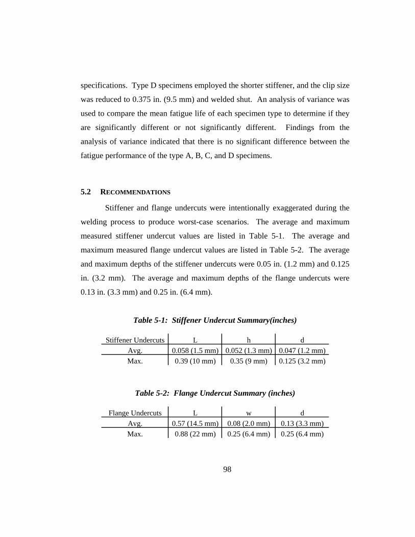
specifications. Type D specimens employed the shorter stiffener, and the clip size

was reduced to 0.375 in. (9.5 mm) and welded shut. An analysis of variance was

used to compare the mean fatigue life of each specimen type to determine if they

are significantly different or not significantly different. Findings from the

analysis of variance indicated that there is no significant difference between the

fatigue performance of the type A, B, C, and D specimens.

5.2 RECOMMENDATIONS

Stiffener and flange undercuts were intentionally exaggerated during the

welding process to produce worst-case scenarios. The average and maximum

measured stiffener undercut values are listed in Table 5-1. The average and

maximum measured flange undercut values are listed in Table 5-2. The average

and maximum depths of the stiffener undercuts were 0.05 in. (1.2 mm) and 0.125

in. (3.2 mm). The average and maximum depths of the flange undercuts were

0.13 in. (3.3 mm) and 0.25 in. (6.4 mm).

Table 5-1: Stiffener Undercut Summary(inches)

Stiffener Undercuts L h dAvg. 0.058 (1.5 mm) 0.052 (1.3 mm) 0.047 (1.2 mm)Max. 0.39 (10 mm) 0.35 (9 mm) 0.125 (3.2 mm)

Table 5-2: Flange Undercut Summary (inches)

Flange Undercuts L w dAvg. 0.57 (14.5 mm) 0.08 (2.0 mm) 0.13 (3.3 mm)Max. 0.88 (22 mm) 0.25 (6.4 mm) 0.25 (6.4 mm)

98

99

The values listed in Table 5-1 and Table 5-2 are larger than measurements

published in recent literature. In their study, Janosch and Debiez measured the

average depth of undercutting at the weld toe. The largest average undercut depth

reported was 0.03 in. (0.76 mm). Undercuts larger than 1 mm were typically

rejected by weld inspectors (Iida et al., 1998).

With good welding practice, fillet welds can be wrapped around the

stiffener with minimal undercutting as documented in the FHWA tour of steel

bridge fabrication.

A 1.5 in. (38 mm) clip opening allowed adequate space to maneuver the

welding gun to wrap the weld around the stiffener. Depending on the size of the

web-to-flange welds, a clip size of 1.0 in. (25.4 mm) may be sufficient.

Research presented in this project showed that stiffener and flange

undercuts do not impact fatigue life in the presence of flange forces. The effect of

cross-frame forces in the stiffener upon the fatigue performance of the wrapped

weld detail was not considered in this research. However, assuming that the

stiffener forces are negligible, it can be restated that wrapping the weld around the

stiffener has no impact upon fatigue life.

100

CHAPTER 5 Summary and Conclusions .................................................. 97

5.1 Evaluation of Test Results ......................................................... 97

5.2 Recommendations ..................................................................... 98

Table 5-1: Stiffener Undercut Summary(inches) ................................................. 98

Table 5-2: Flange Undercut Summary (inches) ................................................... 98

Figure 5-1: Stiffener and Flange Undercuts ......................................................... 97

100

Bibliography

Massarelli, P. J., Baber, T. T. Fatigue Reliability of Steel Highway Bridge Details.

Final Report, Virginia Department of Transportation and the University of

Virginia. Commonwealth of Virginia, 2001.

Nussbaumer, A., Imhof, D. On the Practical Use of Weld Improvement Methods.

Prog. Struct. Engng Mater, John Wiley and Sons, Ltd.Vol. 3, pp. 95-105,

2001.

Verma et al. Steel Bridge Fabrication Technologies in Europe and Japan. FHWA

Report-PL-01-018, Washington, D.C.: The Federal Highway Association,

March 2001.

AASHTO. The AASHTO LRFD Bridge Design Specifications, 2nd Edition. USA:

American Association of State Highway And Transportation Officials, 1998.

AISC. Manual Of Steel Construction, LRFD, 2nd Edition. USA: American

Institute of Steel Construction, 1998.

K. Iida et al. Fatigue Strength of Butt-Welded Joint With Undercut. Welding in

the World, Vol. 39, No. 5, pp. 35-44, 1998.

Janosch, J.J., Debiez, S. Influence of the shape of undercut on the fatigue strength

of fillet welded assemblies, application of the local approach. Welding in the

World Vol. 41, No. 4, pp. 350-360, 1998.

101

Skaloud, M., Roberts, T.M. Fatigue Crack Initiation and Propagation in Slender

Webs Breathing Under Repeated Loading. Journal of Construct. Steel Res.,

Vol. 46, No. 1-3, pp. 417-419, 1998.

Miki. C., Tateishi, K. Fatigue Strength of Cope Hole Details in Steel Bridges.

International Journal of Fatigue, Vol. 19, No. 6, pp. 445-455, 1997.

Texas Department of Transportation. Fax Transmission: CSTM-Structural,

Fracture Critical Defect Repair Procedure #TI0003. TxDOT, 1996. Fax Date:

August 1, 2001.

ANSI, AWS, AASHTO. Bridge Welding Code D1.5-95. USA: American Welding

Society and the State Highway And Transportation Officials, 1995.

Terasaki et al. Effect of Undercut and Nonpropagating Crack Depths on Fatigue

Strength of Welded Joint. Journal Japan Institute of Metals, Vol. 58, No. 10,

pp. 1149-1155, 1994.

Onozuka et al. Fatigue Strength of Fillet Welded Joints with Undercuts.

Proceedings of the Third International Offshore and Polar Engineering

Conference, Singapore, June 6-11, Vol. 4, pp. 199-205, 1993.

Skorupa, M., Scorupa, A. Significance of Crack Initiation Period in Structural

Steel Welds. OMAE-ASME, Vol. III-B, pp. 715-720, 1993.

Petershagen, H. The influence of undercut on the fatigue strength of welds, a

literature survey. Welding in the World, Vol. 28, No. 7/8, pp. 114-125, 1990.

102

Dijkstra et al. The Fatigue Behavior of Welded Splices with and without Mouse

Holes in IPE 400 and HEM 320 beams. Weld Failures, November 1988.

Gurney, T. R. Fatigue of Welded Structures, 2nd Edition. Cambridge: Cambridge

University Press, 1979.

The Lincoln Electric Company. The Procedure Handbook Of Arc Welding, 12th

Edition. USA: The Lincoln Electric Company, 1973.

Gurney, T.R. Effect of Peening and Grinding on the Fatigue Strength of Fillet

Welded Joints. British Welding Journal, December 1968.

Ruge, J., Woesle, H. Results of Fatigue Investigations, abstract of Ergebnisse von

Dauerfestigkeitsuntersuchungen published in Die Schweisstechnik im Zeichen

Neuzeitlicher Verfahren und Werkstoffe. Deutscher Verband fur

Schweisstechnik, pp. 59-68, 1962.

Texas Department of Transportation. Plate Girder Details. Web Address:

ftp://ftp.dot.state.tx.us/pub/txdot-info/cmd/cserve/standard/bridge/spgdstde.pdf 2001.