Section VI Methodological and conceptual considerations

20 The longitudinal study of motor development: methodological issues

WOLFGANG SCHNEIDER

INTRODUCTION

In most areas of human development, the majority of research findings have been based on cross-sectional designs. Such studies focus on developmental differences among various age groups and ignore developmental changes within individuals over age, which means that they cannot be considered tobe truly developmental (cf. McCall, 1977; W ohlwill, 1980). Changes occurring over time within organisms can be assessed only via longitudinal approaches.

The main theme of this chapter is a discussion of methodological issues of longitudinal studies in the area of motor development. In my view, most methodological issues related to the longitudinal assessment of motor development can be easily generaüzed to other areas of human development. Thus, the reader should keep in mind that, while the various methodological problems considered in this chapter are always ünked to topics of motor development, they are not confined to this area of research.

A first general problern concems the defintion of a longitudinal study. As I noted elsewhere (Schneider, 1989), the term longitudinal does not describe a single method but a large variety of methods. The spectrum of methods ranges from single case studies in time-series arrangements to broad-band panel designs including numerous meas­urement points and thousands of subjects. The only common denomi­nator of longitudinal researcb is variation of time and repeated observation of a given entity (cf. Baltes & Nesselroade, 1979).

A closer Iook at the contributions to this book reveals that the diversity of longitudinal approacbes is also well represented in tbe domain of motor development. For example, it seems obvious that

318 W. SCHNEIDER

longitudinal studies on the emergence of fetal movements (cf. Prechtl, Chapter 3, this volume) take place within a limited period of time. Sirnilarly, longitudinal assessments of spoon use in small children (see Connolly & Dalgleish, Chapter 12, this volume) or studies on the development of early motor functions (cf. von Hofsten, Chapter 7, Woollacott, Chapter 6, this volume) usually do not span time intervals larger than a few months. In contrast, longitudinal studies concerning the irnplications of early risk factors on subsequent motor development typically require designs including large numbers of subjects and variables as weil as time schedules spanning many years (see Largo, Kundu & Thun-Hohenstein, Chapter 16, this volume; Michelssou & Lindahl, Chapter 17, Touwen, Chapter 2, this volume).

Given these definitional problems, the methodological issues dis­cussed in the remainder of this chapter may be relevant for some but not for all types of longitudinal studies. Before entering this discussion, I want to summarize the structure of this chapter. As a first step, possible rationales for longitudinal research are described briefly. According to these rationales, two major types of longitudinal study on motor development can be identified. The methodological issues discussed in the next sections of this chapter tap two explanatory statistical approaches that may not be generally weil known but that I consider to be relevant for longitudinal research. Illustrative examples from our own Munich Longitudinal Study on the Genesis of Individual Competencies (LOGIC; see Weinert & Schneider, 1987, 1989) will be used to demoostrate the advantages of these relatively new statistical tools, and an attempt will be made to show how these approaches can be applied to the longitudinal studies presented in this volume.

BASIC RATIONALES FOR LONGITUDINAL RESEARCH

According to Baltes & Nesselroade (1979), the basic goals of lon­gitudinal enterprises concern both the description and the explanation of human development. There are three rationales that relate to the description of development: (1) identification of intraindividual change; (2) identification of interindividual differences in individual change, and (3) the identification of interrelationships among classes of behaviour during development. Two further goals concem the explanation of development: (4) analysis of causes of intraindividual change, and (5) the analysis of causes of interindividual differences in intraindividual change. I now add another goal related to the explanation issue and not explicitly included in this classification system, namely (6) the predic­tion of individual differences in one domain from individual differences

Methodological issues 319

in another domain. Studies illustrating this category include, for example, longitudinal projects exploring the impact of early risk factors (domain A) and later motor skills (domain B). These studies are clearly longitudinal in perspective in that the same individuals are tested repeatedly but do not necessarily include aspects of intraindividual change in a specific variable.

There seems to be a general agreement in the developmentalliterature that two basic types of longitudinal enquiry can be used to reach the five goals listed above (cf. Appelbaurn & McCall, 1983). One ba~c aspect of longitudinal enquiry concerns what Wohlwill (1980) called the 'developmental function'; that is, the average value of a dependent variable plotted over time. Typical examples drawn from longitudinal research on motor development include growth curves concerning the development of speed or physical strength and depicting the continuity versus discontinuity of these variables over time.

The second realrn of longitudinal enquiry concerns the issue of individual differences: the question here is whether individual subjects maintain approximately the same relative rank ordering within their group at one age as they do at another (McCall, 1977). In this type of enquiry, the rnajor issue is how stable or unstable individual differences between individuals remain over time. Note that the issue of stability vs instability of individual differences over time is conceptually iodependem from the issue of continuity vs discontinuity of a develop­mental function: for exarnple, it is tbeoretically possible that a monoto­nic, linear increase in the average dependent variable over time is accornpanied by a high degree of instability of individual differences in this variable. More specifically, the fact that a linear increase in motor coordination skills can be found over the preschool years does not exclude the possibility that individual differences in performance are not preserved over this time interval. As noted by Appelbaum & McCall {1983), tbe relationship between both concepts is always an empirical question. Longitudinal researchers have often overlooked the fact tbat the developmental function and the stability of individual differences over time represent two separate aspects of the same problern (see Hopkins, Beek & Kalverboer, Chapter 21, this volume, for a more systematic treatment of this topic).

IMPLICA TIONS FOR METHODOLOGY

How do the different rationales and types of enquiry relate to the gross classification of longitudinal studies on motor development as described above? That is to say, what are the implications for the small time scale, microanalytical longitudinal studies typically conducted within a few

320 W. SCHNEIDER

months as compared to !arge time scale longitudinal studies on motor development usually spanning several years? The answer is certainly unsatisfactory for those researchers dealing with the large-scale studies because the possible types of data analysis are more restricted and methodological problems are more apparent in these studies than in microanalytical studies.

In principle, rationales (1) to (5) described above can be easily realized in the latter type of study. As these studies usually include identical measures assessed repeatedly over relatively short periods, descriptive as weil as explanatory analyses of intraindividual change over time (i.e. assessments of the developmental function) can be conducted without problems. The precondition for the analysis of change scores is that the same measurement instruments are used over time, a criterion certainly met in most microanalytical studies. Mor­eover, analyses referring to the individual difference approach which emphasize the stability Iinstability issue are equally possible.

The situation is more complicated in the case of large-scale studies spanning several years. Many test instruments used in longitudinal studies with children are designed for only a restricted age range. As a consequence, parallel measures tapping the same theoretical construct (e.g. motor coordination skills) for different age periods are usually included in long-term longitudinal studies. Although Goldstein (1979) discussed the possibility of constructing a common scale for different instruments by using various transformation procedures, this allows only for the assessment of relative change; that is, for a comparison of subgroups of a given population. There is no doubt that the use of different measures tapping the same construct severely restricts the analysis of the developmental function.

But even if the same measurement instrument is used on each occasion, its theoretical meaning may differ (cf. Magnusson, 1981). A variable may appear to be the same at various ages when in fact it is not. For example, there is little doubt that crawling has a different meaning for a 9 month old child than it has for the same child at age 4 years. Thus, assessing long-term intraindividual change in this variable would not make much sense. Whereas the same instrument can be used at all ages with certain measurements such as height or weight, this is not true for the majority of measures concerning motor development in children.

It appears, then, that large-scale longitudinal studies on motor development are of only limited value regarding the assessment of intraindividual changes over time (i.e. the developmental function). Researchers involved in large-scale studies need to focus on interin­dividual differences.

In the remainder of this chapter, I concentrate on explanatory approaches to the study of the developmental function as weil as to the

Methodological issues 321

analysis of interindividual differences. The growth curve rnodels de­scribed in the next section tap aspects of intraindividual change and are particularly useful for rnicroanalytical studies on motor developrnent. On the otber band, structural equation rnodelling procedures (to be discussed in tbe next section) refer mainly to tbe interindividual differences approach and tberefore seem particularly relevant to large­scale studies on motor development.

THE ANALYSIS OF INTRAINDIVIDUAL CHANGE OVER TIME

As described in more detail by Rogosa (1988), there are numerous mytbs about longitudinal research that have been addressed and debunked in recent rnethodological studies. One fundamental mis­understanding concems the measurernent of intraindividual change over time, a misunderstanding that has plagued tbe social sciences for rnore than two decades. It is necessary to surnrnarize tbis problern briefly before moving towards tbe analysis of intraindividual change using sopbisticated statistical tools.

Problems with measuring change

Since the dassie article by Cronbach & Furby (1970), researchers using longitudinal studies have been wamed repeatedly of tbe hazards of change scores. These warnings did not refer to the use of change scores in group analyses, for example, analyses of variance (ANOVAs): it can be demonstrated easily that repeated measures of ANOV As using pretest-posttest raw scores and analyses of variance based on posttest­pretest change scores yield identical results (cf. Maxwell & Howard, 1981; Nunnally, 1982). Rather, tbe warnings concemed tbe use of difference scores for tbe assessment of individual change. According to a widespread belief, individual change scores are unreüable, rnisleading and unfair ( cf. Rogosa, 1988).

The good news for longitudinal researchers struggüng with tbe problern of how best to assess individual change over time is that such problems have been overestimated in the past. Methodological papers written in defence of the difference score have accumulated over tbe last few years (cf. Rogosa, Brandt & Zimowski, 1982; Bryk & Raudenbush, 1987; Rogosa, 1988). In these papers, it was shown that difference scores represent unbiased estimates of true change, and that the traditional objections (e.g. unreliability, unfaimess, bias tbrough re­gression towards the mean) do not generally hold.

For example, Rogosa et al. (1982) demonstrated tbat traditional tabulations of the reüabiüty of the difference score (e.g. Linn & Sünde,

322 W. SCHNEIDER

1977) are incomplete. More comprehensive analyses revealed that the reliability of the difference score is not generally low: low reliability scores will be obtained only when individual growth rates vary little across subjects. Reliability indicates the accuracy with which subjects can be ranked on the growth rate function on the basis of their difference scores, whether the estimates of the growth rate function are precise or not. The important implication is that low reliability does not necessarily indicate Iack of precision. In other words, low reliability of difference scores does not predude meaningful assessment of individual change. The reliability of the difference score is respectable when considerable individual differences in rates of intraindividual change are present (see Rogosa & Willett, 1983).

There is little doubt that the importance of 'regression towards the mean' effects for the study of change has been similarly overestimated in the Iiterature (for critical reviews, see Nesselroade, Stigler & Baltes, 1980; Rogosa, 1988). The traditional meaning of these effects is that, on average, one is doser to the mean at time 2 than at time 1. Nesselmade et al. (1980) however, provided evidence that the common belief that measurement error necessarily produces a regression effect that makes it impossible or very difficult to measure individual change properly is not correct in the case of multiwave data.

In summary, the often cited defi.ciencies of the difference score are more illusory than real. lt should be noted, however, that several possibilities for improving the difference score do exist. The most common one is to supplement the information on a single individual by the information on all individuals in a given sample: in this case, between-person information is used to improve the estimate of intrain­dividual change (see below).

In the following, the focus will be on Bayesian methods applied to the estimation of individual growth curves which represent an impor­tant component of more recent models of individual growth (for a detailed discussion of other improved difference scores, see Rogosa et al., 1982). In particular, Bryk & Raudenbush's (1987) two-stage model of individual growth seems to represent one of the most prornising approaches to the study of change. The rationale of this procedure is provided in the next section.

Application of hierarchical linear models to assessing change

Recent developments in the statistical theory of hierarchical linear modelling (HLM) enable an integrated approach for studying various aspects of individual change. The model presented by Bryk & Rauden­bush (1987) allows the assessment of the structure of growth, examining

Methodological issues 323

the reliability of instruments for measuring both initial status and change, exploring correlates of entry status and change, and for testing hypotheses about the effects of theoretically relevant backgrouod variables. Because of its two-stage character, this conceptuaüzation of growth is usually referred to as a hierarchical linear model. At stage 1, each individual's observed developmeotal chaoges are conceived of as a function of an individual growth curve or trajectory plus random error. At stage 2, the assumption is that the individual parameters deterrnining the individual growth curve vary as a function of certain characteristics of the individual's background or environment (e.g. sex or social dass).

The within-subject model estimated at stage 1 can be represented as a polynomial of any degree. For the sake of clarity, I chose a linear growth rate model to illustrate the logic of the statistical estimation procedure of HLM. See Bryk & Raudenbush (1987) for a more detailed aod technical illustration. Accordingly, the within-subject model equa­tion explaining the individual outcomes at time i becomes:

(20.1)

for i = 1 to n subjects observed on t occasions. The parameter a;.

represents the age of subject i at time t, :Ir; denotes the growth curve parameter for subject i, and R;, is the random error, assumed to be normally distributed with a mean of zero and some covariance structure S. Note that the intercept n 0; and the linear rate of growth n 1; deterrnine the growth curve for each subject.

In a next step, a between-subject model is formulated to represent the variation of growth parameters across individuals, thereby exploring whether the individual growth parameters are a function of measures of background characteristics. The simpüfied between-subjects model based on the assumpcion of linear growth rates and including just one background variable, X;, is then given by:

(20.2a)

aod

(20.2b)

In the equations (20.2a) aod (20.2b), the parameters U0; and U 1;

represent random increments to the individual growth parameters. As Bryk & Raudenbush (1987) point out, combining equations (20.1)

and (20.2) yields a single linear model,

(20.3)

with

(20.4)

324 W. SCHNEIDER

Equation (20.3) represents a Standard linear regression model with an intercept, ß00 , and three predictors, namely the between-subjects variable, X;; age, ait ; and the interaction term, X ;a;, . The new error term, e;" consists of two different components: one component depends on the random increments to the individual growth parameters, U0 ; + U 1;a;" and the other component represents the random error, R;,.

As regards the model assumptions, it is important to note that both the individual outcomes, Yit, and the growth parameters, 1tJ.; are assumed to be normally distributed. In order to facilitate measurement of change, a common metric of the outcome data collected at each measurement point, in logits, is generated by HLM. As growth curve modeHing requires that the outcome data collected at each time point be measured on a common metric, so that changes across time reflect growth and not changes in measurement scale, item response theory is used to calculate a logit function which models the Iogs of ratios of multinomial probabilities.

A detailed description of the model estimation procedure is given by Bryk & Raudenbush (1987). lts logic is as follows. First, an individual's growth rate (n1) is estimated by means of ordinary Ieast-squares procedures. Next, a weighted Ieast-squares regression procedure is used to estimate the between-subject model, yielding a second estimate of individual growth (n2) based on the value of each subject's background variable. In a last step of analysis, empirical Bayes estimation of individual growth curves provides a composite estimator (n3) which is an optimally weighted average of 1t 1 and 1t2 • The weights of this estimator,

W; = T /(T +V;),

have substantive interpretability in that they represent only the ratio of the parameter variance in the growth rates, T, to the total variance, T +V; (V; is the error variance). This ratio is analogous to a reliability coefficient, where the 'true score' variance (T) is compared to the observed score variance (T + V;).

As pointed out by Bryk & Raudenbush (1987), the influence of an individual's time-series data (as captured by the within-subject model) on the composite Bayes estimator thus depends on the reliability of the individual outcome estimate. When this is highly reliable, the HLM estimate for an individual's growth rate will depend on the individual growth curve data. When this is unreliable, however, the HLM estimate will be based primarily on the background data. Thus, HLM uses whatever strength exists in the data to form its composite Bayes estimator, typically yielding smaller mean squared errors than do estimators based on data either from individuals or from groups.

Methodological issues 325

To demoostrate the possibilities of HLM, an illustrative example that is based on data collected in LOGIC (cf. Weinen & Schneider, 1987, 1989) will be presented.

Illustrative example

The sample of the LOGIC study consists of about 200 children who were first tested in late 1984 when they were almost 4 years old. Since then, children have been seen on a regular basis every year, with an average time interval between adjacent measurement points of ap­proximately 12 months. The test instruments administered in these sessions include various measures of intellectual development such as tests of verbal and non-verbal intelügence, and experimental tasks assessing memory skills. Measures assessing children's social com­petencies (e.g. social anxiety, self-concept, moral judgement, and role-taking abilities) were additionally included to explore possible interrelationships between aspects of intellectual and social com­petencies in early childhood.

Moreover, a test of motor abilities (MOT 4-6; see Zimmer & Volkamer, 1984) was also given during each of the first 3 years of the study, a measure of central relevance for our illustrative example. As emphasized by the test authors, the MOT 4-6 attempts to assess a broad variety of motor skills including sense of balance, agility, accuracy of movements, and coordination skills. The test was ad­ministered individually, and scores of 0, 1 and 2 could be given for each of the 17 items, thus yielding a maximum score of 34. A total of 174 children was tested on all three occasions, which were approximately equally spaced throughout the 3 years of assessment. These data are considered in the following analyses.

In addition to the motor test data, a few background variables are also included in the growth curve analyses. First descriptive analyses concerning the developmental function of motor skills revealed that changes over time seemed to vary as a function of sex and age group (split according to the median of the age distribution). Fig. 20.1 shows the mean developmental changes over time, as a function of both sex and age group. As seen in Fig. 20.1, sex differences were not remarkable at the age of 4 years (wave 1) but seem to increase over the years, with girls improving at a faster rate than boys. On the other hand, mean differences between the subsamples of younger and older subjects (mean age difference: 5 months) were pronounced at the very beginning of the study and appeared to fade out later.

The last variable to be considered as a background characteristic was verbal IQ as measured by the Hannover-Wechsler lntelügence Test for Preschool Children (HA WIV A; Eggen, 1978). As several items of the

326 W. SCHNEIDER

25

w ~20 ü Cl)

~ 15 Cl)

~ Cl)

;!: 10 0:: 0 I- 5 0 ~

0 'MVE 1 'MVE 2 WIWE 3

DMALE ~FEMALE

25 w 0::

8 20 Cl)

~

~ 15

~ Cl)

;!: 10 0:: 0 I-0 5 ~

0 'MVE 1 'MVE 2 ~VE3

CJ YOUNGER ~OLOER

Fig. 20.1. Developmental changes in motor task sum scores as a function of sex (top) and age (bottom) group.

MOT 4-6 required very detailed instructions not easy for preschoolers to understand, our assumption was that verbal comprehension skills could influence performance on the MOT 4-6. Indeed, verbal in­telligence (sirnilar to age and sex) bad significant bivariate relations with early motor skills and with invidicual change in this variable. As a consequence, these variables were used in the between-subjects model of our illustrative example.

Examining individual growth First in the HLM analysis the degree of the polynomial to be fitted has tobe identified. For the sake of clarity, I consider only the simple linear

Methodological issues 327

Table 20.1. Estimated mean growth parameters (/ixed effects)

Mean growth parameter Standard

Dependent variable estimator error z p

Motor Sum Score lntercept 15.15 0.90 16.87 < 0.01 Linear trend 3.70 0.57 6.49 < 0.01

Table 20.2. Estimated variance components (random effects)

Estimated

Dependent variable par~eter

x2 d.f vanance p

Motor sum square lntercept 10.39 691.30 172 < 0.01 Linear trend 0.41 149.22 173 < 0.10

individual growth model described above. Next the mean growth curve for the entire sample is identified. Here, the interest is in determining the simplest mean growth model that is consistent with the data. Table 20.1 presents the results of this analysis. A simple Z test is available by computing the ratio of each estimate to its Standard error. As can be seen from T able 20.1, results for both the intercept and growth rate parameters are significant, indicating that both parameters differ from zero and are necessary for describing the mean growth curve.

Next, we explored the nature of the deviations of the individual growth curves from the mean trajectory. Results of this analysis are given in Table 20.2. As regards the estimated parameter variance in the intercept, the significant chi-squared statistic indicates that children vary significantly in their initial status. On the other band, the hypothesis of no interindividual variation in linear growth rates has to be accepted, as the chi-squared statistic obtained for the estimated parameter variance in the growth curve component only approaches significance. Thus, the observed variation among the individual motor skill growth rates does not indicate reliable interindividual differences in change rates.

Co"elates of change and status

A subsequent step of analysis concerned the relations among back­ground variables, entry status, and growth rate. Table 20.3 presents results from this analysis. The parameters can be interpreted in exactly the same way as in ordinary regression analysis. Results concerning the

328 W. SCHNEIDER

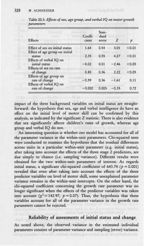
Table 20.3. Effects of sex, age group, and verbal!Q on motor growth parameters

Stan-Coeffi- dard

Effects cient error z p

Effect of sex on initial status 1.64 0.54 3.01 <0.01 Effect of age group oo ioitial

status 2.35 0.55 4.27 <0.01 Effects of verbal IQ oo

initial status -0.02 0.01 -2.46 <0.05 Effects of sex on rate

of change 0.80 0.36 2.22 <0.05 Effects of age group oo

rate of change -0.59 0.36 -1.61 0.11 Effects of verbal IQ oo

rate of change -0.002 0.005 -0.35 0.72

impact of the three background variables on initial status are Straight­forward: the hypothesis that sex, age and verbal intelligence do have an effect on the initial Ievel of motor skill can be confirmed by this analysis, as indicated by the significant Z statistic. There is also evidence that sex significantly affects children's rates of growth, whereas age group and verbal IQ do not.

An interesting question is whether our model has accounted for all of the parameter variance in the within-unit parameters. Chi-squared tests were conducted to examine the hypothesis that the residual differences across units in a particular within-unit parameter ( e.g. initial Status), after taking into account the effects of the three stage 2 predictors, are due simply to chance (i.e. sainpling variance). Different results were obtained for the two within-unit parameters of interest. As regards initial status, a significant chi-squared coefficient of 643.74 (p = 0.001) revealed that even after taking into account the effects of the three predictor variables on Ievel of motor skill, some unexplained parameter variance remains in the within-unit intercepts. On the other band, the chi-squared coefficient conceming the growth rate parameter was no Ionger significant when the effects of the predictor variables was taken into account (X2 = 142.97, p = 0.07). Thus, the hypothesis that these variables account for all of the parameter variance in the growth rate parameters cannot be rejected.

Reliability of assessments of initial status and change

As noted above, the observed variance in the estimated individual parameters consists of parameter variance and sampling (error) variance.

Methodological issues 329

Following classical measurement theory, the ratio of the 'true' para­meter variance to the 'total' observed variance can be conceived of as the reliability of the individual data estimate. In the illustrative example, the reliability of the initial status estimates was 0.74, and the reliability of the growth rate estimates was 0.07. The result for the growth rate estimates indicates that there is little variation in the growth rate parameters over time: while children's motor skills are steadily develop­ing, rate of development is relatively constant across individuals. This is obvious from Fig. 20.2 showing a selection of individual time paths from a random group of ten children. Although individual differences in entry status are considerable, individual differences in growth rates are negligible.

As noted earlier, the procedures just illustrated generalize directly to more complex growth models. In the illustrative example based on three measurement points, the fit of a quadratic model to the data can also be examined. Results of a trend analysis revealed, however, that a linear trend hypothesis describes our data best, at least as far as the mean growth curve is concerned (cf. Weinert & Schneider, 1989). As pointed out by Bryk & Raudenbush (1987), it is important to note that the mean growth curve and the individual growth curves can have different forms. For example, in fitting a quadratic model to the data, one might find

30

Cl) 25 1-

8 -' ~ Cl) 20 ~ ::::> Cl) w a: 1-Cl) 15 w 1-

10

~'~·------------------------~r YEAR 1 YEAR3

Fig. 20.2. A configuration of randomly selected individual time paths exhibiting very slight individual differences in change.

330 W. SCHNEIDER

that some individual growth curves with positive curvatures cancel out others with negative curvatures. In this case, a linear model would be a fine description for the group development but inadequate for describ­ing individual growth. Visual examination of the individual time-series is thus suggested to identify models that can be fitted to the data.

Concluding comments on HLM

In the illustrative example, I have tried to highlight some of the specific strengths of HLM relevant to the study of motor development. HLM provides an integrated approach based on a two-stage, hierarchical model. This approach not only allows for studying the structure of individual growth and estimating statistical and psychometric properties of collections of growth curves, but also for assessing the adequacy of between-subject models by estimating the reduction in unexplained parameter variance as demonstrated in the illustrative example. In addition, HLM can be used (a) to assess the reliability of measures for studying both entry status and change, (b) for estimating the correlation between entry Status and rates of change, and (c) for predicting future individual growth (for details, see Bryk & Raudenbush, 1987). While HLM requires multiwave data, the approach is quite flexible in that the number and spacing of observations may differ across subjects.

In my view, one of the most important advantages of the HLM programme is that it capitalizes on any strengths in the available data; that is, if the individual growth curve estimates are reliable, HLM will weight them heavily. If the individual growth curve estimates are not reliable, the model will rely more on information from mean growth curves that are conditioned on available background data.

THE ANALYSIS OF INDIVIDUAL DIFFERENCES OVER TIME

Longitudinal research focusing on individual differences is concemed primarily with the issue of stability and predictability over time. For many years, regression-type statistical models have been used to describe and explain the longitudinal stability or lability of individual differences in various domains. Multiple regression analyses are typi­cally based on correlacion coefficients or covariance structures. The goal is to predict individual differences in an observed criterion variable from

. a variety of predictors that could either consist of identical measures assessed at an earlier point in time or represent conceptually different variables. One of the basic problems with this approach has been that, while the underlying statistical model assumes independence of predic­tor variables, the predictors used in regression analyses are often highly

Methodological issues 331

intercorrelated. As a consequence, the resulting estimates are frequently biased. Another drawback of this statistical model is that nothing is known about possible interrelationships among predictor variables: they are all treated as having the same explanatory status.

The latter is not true for a more sophisticated regression procedure, namely path analysis regression based on observed variables. The advantage of this procedure is that more elaborated cause-effect interrelationships among predictor variables can be estimated and tested. However, these path models can get very complex and difficult to interpret in the case of numerous observed variables, as is typically true for large-scale longitudinal studies on motor development.

The situation changed dramatically with the publication of another elaboration of the regression approach; that is, structural equation modelling (SEM) procedures using latent variables, also called a 'second generation' development of causal modelling (Schneider, 1986). Com­puter programs based on this approach bave been around since the late 1970s and early 1980s (e.g. the linear structural equation (LISREL) model developed by Jöreskog & Sörbom (1984)). Causal modeHing and the application of SEM techniques are enjoying increasing popularity among behavioural scientists analysing data relevant to human develop­ment and change. As several introductions into the SEM approach are available (e.g. Bentler, 1980, 1985; Jöreskog & Sörbom, 1984; Alwin, 1988; Lohmöller, 1989; see also tbe first issue of Chüd Development (1987) for a detailed description and for applications of SEM proce­dures), there is no need to discuss the principles of SEM in much detail in this chapter. lnstead, I focus on a short description of the rationale of tbe approach and its advantages over traditional regression procedures.

Advantages of SEM procedures

A typical feature of all SEM techniques using latent variables is the distinction between a measurement model and a structural model. While tbe measurement model defines the relationships between observed variables and unmeasured hypothetical constructs representing the observed variables, the structural equation model (i.e. 'causal' model) is used to specify the causal links among the latent variables. Thus, a factor analytical approach is used to create the latent variables, whereas a regression-type approach is used to analyse the structural relations among tbe latent variables. As general interest is more in causal/ structural relationships among tbeoretical constructs than in relationships among fallible observed variables, tbe logic behind the distinction used in the SEM procedures makes much sense. While SEM techniques using latent variables can be applied principally to cross-sectional data, they seem particularly promising when used witb longitudinal data.

332 W. SCHN EID ER

In short, their major advantages- as compared to traditional regres­sion analysis - are as follows.

(1) A verbal theory has to be translated into a mathematical model that can be estimated.

(2) Causal relationships are estimated on the Ievel of theoretical constructs.

(3) The distinction between a measurement model describing the relationships among observed variables and a structural model describing interrelationships among theoretical constructs also allows for a separate estimation of measurement errors in the observable and specification errors in the structural part of the model: large specification errors usually indicate that the causal model is not completely specified and that theoretically impor­tant predictor variables are missing.

(4) Another advantage is that a distinction between the reliability of measured variables and the stability of structural relations is possible (for more details, see Rudinger et al., 1989).

(5) Several so-called goodness-of-fit tests exist that detect the degree of fit between the causal model and the data to which it is applied. Causa} models are said to be confirmed when the goodness-of-fit parameter indicates better-than-chance fit between the model and the data.

(6) Identical structural models can be specified for different samples ( e.g. different age groups, or children at risk vs normal samples) to test the generalizability of a given theoretical model.

(7) While SEM procedures generally operate on correlation or covariance matrices, mean structures can also be considered. This means that in the case of multiple group comparisons relative changes in the means of latent variables over time can also be assessed.

Illustrative example

The data for the illustrative example demonstrating the utility of the SEM approach for the study of motor development are again taken from the LOGIC study. The target group consisted of those 174 children with complete data on the MOT 4-6 and two intelligence tests (the HA WIVA by Eggert (1978) and the Columbia Mental Maturity Scale (CMMS) by Burgemeister, Blum & Lorge (1972)) for the first 3 years of the study. The research question of core relevance concerned the relationship between early intellectual and early motor development.

Methodological issues 333

Verbal tbeory

Admittedly, our knowledge concerning tbis relationship and its course over the preschool and kindergatten years is extremely scanty. None the less, there is reason to assume that young children's coordination skills and intellectual abilities may be related. Fine motor tasks such as tapping or balance are complex activities that require not only motor regulation skills but also cognitive information-processing abilities (cf. Bös, 1987). More specifically, motor coordination skills seem to be linked to aspects of visual perception (spatial imagination skills or aspects of (motor) memory). Cognitive factors seem particularly impor­tant in preschool children's motor coordination skills: fine motor tasks require an enormous amount of conscious, self-regulatory actions by 3 to 4 year olds.

Thus the first assumption, our developmental trend hypothesis, is that the strength of the interrelationship between motor and intellectual abilities will decrease with increasing age. The ability to control complex movements will no Ionger depend on the amount of mental effort as soon as motor actions become increasingly automatized.

A second assumption (reciprocal causality hypothesis) concerned mutual influences between the two theoretical constructs. Analyses of reciprocal effects and aspects of predorninance are typically framed as 'does construct X cause construct Y or is it just the other way around'. In the illustrative example, the assumption was that the predorninant causal influence should be from intellectual ability to motor coordina­tion skills, at least as far as the early measurement points are concerned. In line with the developmental trend hypothesis that interrelations between cognitive abilities and motor coordination skills should de­crease with increasing age, the issue of reciprocal causality should be of minor importance when children enter elementary school.

Model specification

The most parsimonious model describing developmental trends in both constructs is depicted in Fig. 20.3. In this model, the latent variables are represented by circles, whereas the observed indicators are given as squares. There are two observed variables per construct: for each measurement point, indicators of verbal and non-verbal intelligence were combined to represent the intelligence construct. Instead of using the sum score of the MOT 4-6, two subcomponents representing fine motor coordination skills and coordination skills including an endur­ance component were chosen for the motor skill construct. In total, the model thus comprised 6 latent variables and 12 observed indicators

The 'independence model' depicted in Fig. 20.3 is parsimonious in that it does not assume any reciprocal causal effects (i.e. path coefficients

334 W. SCHNEIDER

going from motor skill at time 1 to IQ at time 2 or vice versa). This model is equivalent to a first-order autoregressive or simplex model representing the IQ and motor variables as causes of themselves over three points in time. In this model, changes over time are assumed to be independent of prior changes; that is, paths ünking wave 1 and wave 3 variables are omitted. The expectation was that the alternative model representing reciprocal causal effects for the first two waves should fit the data significantly better than the more restrictive 'independence model'.

Estimation and test of the model

Because of space restrictions, this section contains only a brief report on the model estimation procedure (for a more detailed account, see Schneider, 1988). I focus on the analyses based on EQS (Equations: see Bentler, 1985) because a distribution-free estimation procedure is available for this technique. This turned out to be essential because the motor test data from the third year deviated significantly from normality.

In the first step of analysis, it was shown that the 'independence model' did not fit the data. An alternative model including the causal reciprocity relation for the first two waves but still maintaining the simplex structure depicted in Fig. 20.3 seemed to be more compatible with the data structure but also did not fit the data. An acceptable data fit was obtained only when the simplex restriction was given up; that is, when direct causal links between constructs measured at waves 1 and 3 were included in the model.

The results for the final model are given in Fig. 20.4. For the sake of clarity only the interrelations among latent variables are included in the path diagram. As can be seen from Fig. 20.4, the effects of intelligence at wave 1 on later motor coordination skill assessed at wave 2 almost doubles the corresponding effect of earlier motor skills on subsequent intelligence. This finding is in accord with the theoretical assumption concerning reciprocal effects indicating a predominance of intelligence over motor skills for the preschool years. Note that no reliable reciprocal causal effects were found for the later phase of data collection (i.e. the time interval between waves 2 and 3).

The data were also compatible with our developmental trend hypothesis in that the correlations between the IQ and motor skill constructs dropped significantly over time (from 0.64 at wave 1 to 0.25 at wave 3 ). Finally, the dotted path from motor skills at wave 1 to motor skills at wave 3 indicates that the inclusion of this link was absolutely necessary in order to obtain a sufficiently good data fit. Although the autoregressive path coefficients for the motor skill

Methodological issues 335

t [TI

Fig. 20.3. Strucrural equation autoregressive ('independence') model assuming no reciprocal causal effects between intelligence and motor skills.

0.14

Fig. 20.4. EQS structural equation model based on a distribution-free estima­tion procedure that fits the data well.

336 W. SCHNEIDER

construct tumed out to be generally !arge, they did not fully explain the data structure. On the other band, the direct effect of intelligence measured at wave 1 on intelligence assessed at wave 3 was comparably small. Although the omission of this path had negative consequences on data fit, the resulting model still fits the data according to the available goodness-of-fit indicators.

Concluding comments on SEM procedures

There seems to be broad agreement that SEM procedures represent powerful general tools for the analysis of longitudinal data. They seem particularly appropriate in large-scale longitudinal studies on motor development operating on !arge sample sizes where researchers typically struggle with a large nurober of variables assessed at different points in time. As noted above, tbe SEM approach includes the features of traditional regression approaches but is clearly superior because of its flexibility. lt is demanding because researchers are forced to specify their verbal theories and to translate them into corresponding statistical models. lt is not only possible to estimate causal models but also to test them; that is, to evaluate their data fit. Moreover, the goodness-of-fit coefficients for competing causal models can be directly compared.

Recent developments further indicate that in addition to the analysis of correlation or covariance matrices, mean structures can also be integrated. For example, McArdle & Epstein (1987) illustrated the possibilities of a longitudinal model that included correlations, vari­ances, and means and was described as a latent growth curve model. The inclusion of mean structures makes such a longitudinal structural equation model more similar to repeated-measures ANOVA proce­dures. As a consequence, this type of model may also be used to assess the developmental function; that is, group changes in the amount of a latent variable over time.

Despite the several advantages of SEM procedures, they should not be conceived of as panaceas. Several problems with SEM procedures have been addressed in the Iiterature ( e.g. Martin, 1987; Alwin, 1988; Rogosa, 1988). The availability of these techniques offers great potential for abuse. As emphasized by Alwin (1988), in the absence of a well-defined set of tbeoretical assumptions, in the absence of valid indicators of tbeoretical assumptions, in the absence of valid indicators of theoretical constructs, or in the absence of a careful set of procedures fot measurement, these methods may Iead one to meaningless conclu­sions giving the false appearance of importance. lt represents one of the major difficulties for tbe responsible researcher using SEM techniques to assess tbis risk.

Methodological issues

IMPLICATIONS FOR THE LONGITUDINAL STUDIES DESCRIBED IN THIS VOLUME

337

Undoubtedly, the HLM and SEM procedures described above have a wide range of appücability and seern useful for longitudinal studies deaüng with various aspects of rnotor developrnent. In the rernainder of this chapter, I try to illustrate how sorne analyses presented in this chapter could be complemented by these two explanatory approaches.

Tool use by infants The study by Connolly & Dalgleish (Chapter 12, this volurne) represents a microanalytical longitudinal approach focusing on issues of intraindividual change. lt provides an interesting, detailed description of the development of spoon-using skills in four infants. The authors' decision to explore the developrnental patterns with a very srnall sarnple seerns convincing. In their view, the adequacy of nornothetic deveiop­mental approaches assessing the 'average' child is questionable because pooüng data across subjects rnay obscure the underlying processes of change; that is, the phenornenon that different individuals can take different routes to reach the same developrnental end-point. Conse­quently, the emphasis in the Connolly & Dalgleish study is on individual development. For each child, data on various behavioural categories were obtained during an interval of about half a year, resulting in about 20 rneasurernent points per child.

Connolly & Dalgleish chose to analyse the data separately for each child by using orthogonal polynornials. This trend analysis approach seerns appropriate for the analysis of single case data in that it provides a description ofthebest-fit curve (linear, quadratic, or cubic) for the data. The authors correctly refer to the problern that this approach rnay be of questionable value in the case of non-normal data. They also pay attention to the problern that a number of their analyses (more than 300 ANOVAs) are ükely to be significant by chance. Although Connolly & Dalgleish consider the possibility of 'significance by chance' effects when interpreting their findings, their decision rules seern somewhat arbitrary, at least as far as the ignorance of quadratic effects in the data is concerned.

All in all, the single case trend analysis approach presented by Connolly & Dalgleish seems appropriate for a description of individual changes over time. However, its most apparent restriction is that results are difficult- if not impossible- to generaüze across subjects. Accor­dingly, information about the representativeness of findings cannot be obtained. In my view, this dilernrna is solvable by using the HLM approach because the nomothetic and ideographic dimensions can be combined due to the two-stage characteristic of the model.

338 W. SCHNEIDER

How can HLM be used to elaborate on the findings presented by Connolly & Dalgleish? Obviously, the HLM procedure cannot be meaningfully applied to data based on such a smaU sample size (i.e. four subjects). However, it could be used for the analysis of data reported by Connolly & Dalgleish (1989) for two groups of infants. The methods employed in this study were essentially the same as those of Connolly & Dalgleish (Chapter 12, this volume). Application of HLM to these group data could not only lead to an estimate of the 'average' child's skill acquisition but also give information on interindividual differences in intraindividual change. Background characteristics (e.g. sex) could be induded in the analysis to explain the interindividual differences observed.

Of course, the scientific value of such an approach depends on the quality and significance of available background variables. The explana­tory power of the data collected by Connolly & Dalgleish seems restricted in that the mother's influence on the infant's acquisition of tool use was not considered. It should be noted in this regard that Connolly & Dalgleish were not particularly interested in a com­prehensive explanatory approach, and that their emphasis on isolated changes in children's behaviour seems legitimate given their specific research goals. None the less, I think that parameters of mother-child interactions should be induded in future studies on this issue in order to estimate the ecological validity of the laboratory approach.

Motor development in children at risk

As noted earlier, studies dealing with the implications of early risk on later motor development are usually based on large samples of subjects and variables and typically span several years. As a consequence, they represent potential candidates for the SEM approach. In the following, the possibility of complementing data analysis by adding explanatory SEM approaches is discussed briefly using the studies by Largo et al. (Chapter 16, this volume) and Michelsson & Lindahl (Chapter 17, this volume) as illustrative examples.

In the study by Largo et al. (Chapter 16, this volume), the primary goal concerned the description of motor development, with a specific focus on issues of variability and stability in normal development, and on the impact of several pre- and perinatal risk factors on later motor development. Data from two samples of about 100 preterm and 100 fullterm children depicting the developmental course from birth to school entrance were used in this study. Neurological and motor development during the first 2 years of life was repeatedly assessed, and minor congenital anomalies were measured at age 5 years. Further, data

Methodological issues 339

conceming neurological assessment were also collected when children were 4 and 6 years old.

It appears that both HLM and SEM procedures can be used in future analyses of this data. HLM analyses should be restricted to the first 2 years of the study, where information on neurological and motor development are particularly rich; that is, based on a total of seven measurement points. In addition to the correlations reported by Largo et al., analyses of mean change and interindividual differences in intraindividual change could be carried out, using risk status as the crucial background variable.

SEM models could be implemented to link motor and neurological development over the range 0 to 6 years. Information on pre-, peri- and postnatal factors could be used to predict minor congenital anomalies. Given that sample size of each subgroup is not particularly large, data of preterm and fullterm children could be aggregated, and a dummy risk variable could be introduced into the model as an explanatory factor.

One nice aspect of the Zurich Longitudinal Studies described by Largo et al. (Chapter 16, this volume) is that several age cohorts are available. SEM approaches could make use of this advantage, comparing structural features of motor development for samples followed through different decades of this century. Such model comparisons involving different age cohorts could give valuable information on the generality or universality of findings.

Regarding the study by Michelsson & Lindahl (Chapter 17, this volume), sample size does not cause any problems for SEM procedures. The risk group in the Helsinki Longitudinal Study included more than 850 children followed from birth to age 9 years. In addition, a smaller group of normal control children was available. Comprehensive assess­ments were carried out when children were 5 years old, including tests of intelligence and language skill, concentration, and gross and fine motor performance. Assessments at the age of 9 years focused on neurological examinations, including various fine and gross motor functions, and a comprehensive test of motor impairment. In addition, tests of intelligence, language skills, and the reading and spelling were carried out at that particular age.

Michelsson & Lindabi tried to explain the outcomes in the five criterion areas of achievement (i.e. neurological assessment, motor function, language skill, intelligence, and school performance) by using ·Jogistic regression analysis as statistical tool. While this tool is prin­cipally appropriate for the kind of prediction model inherent in the design of the study, it is of restricted value given that it operates on observed variables and cannot consider more than one dependent variable at the same time. The advantages of SEM models seem immediately apparent: (a) tbe distinction between theoretical constructs

340 W. SCHNEIDER

and observed variables representing these constructs could Iead to a considerable reduction in (latent) variables included in the structural equation models; (b) a structural equation model simultaneously including all five criterion areas could be specified, thus allowing for assessing differential effects of early risk factors on the various outcome domains; (c) the same structural equation model could be specified for different risk groups. On the basis of such an approach, multiple group comparisons could be carried out to explore whether the same causal model holds for the different risk groups.

In summary, this short illustration of possible applications of HLM and SEM approaches in the area of motor development has shown that these two procedures can be advantageous when it comes to the explanation of normal and abnormal motor performance. This does not imply, however, that these approaches should be conceived of as panaceas; they certainly cannot compensate for poor-quality data, careless operationalization of major constructs and inappropriate designs.

ACKNOWLEDGEMENT

I am grateful to Merry Bullock for her valuable comments to this chapter.

REFERENCES

Alwin, D. F. (1988). Structural equation models in research on human development and aging. In: K. W. Schaie, R. T. Campbell, W. Meredith & S. C. Rawlings (eds.), Methodological issues in aging research, pp. 71- 170. New Y ork: Springer-Verlag.

Appelbaum, M. I. & McCall, R. B. (1983). Design and analysis in developmen­tal psychology. In: P. H. Mussen (ed.), Handbook of child psychology: History, theory and methods, (3rd edn), vol. 1, pp. 415-476. New York: Wiley.

Baltes, P. B. & Nesselroade, J. R. (1979). History and rationale of longitudinal research. In: J. R. Nesselroade & P. B. Baltes (eds.), Longitudinalresearch in the study of behaviour and development, pp. 1-39. New York: Academic Press.

Bentler, P. M. (1980). Multivariate analysis with latent variables: causal modeling. Annual Review of Psychology, 31, 419-56.

Bentler, P. M. (1985). Theory and implementation of EQS: a Structural equations program. Los Angeles: BMDP Statistical Software Corp.

Bös, K. (1987}. Handbuch sportmotorischer Tests. Göttingen: Hogrefe. Bryk, A. S. & Raudenbush, S. W. (1987). Application of hierarchical linear

models to assessing change. Psychological Bulletin, 101, 147-158. Burgemeister, B., Blum, L. & Lorge, J. (1972). Columbia mental maturity scale.

New York: Harcourt Brace Jovanovich.

Methodological issues 341

Connolly, K. J. & Dalgleish, M. (1989). The emergence of a tool using skill in infancy. Developmental Psychology, 25, 894-912.

Cronbach, L. J. & Furby, L. (1970). How should we measure 'change'-or should we? Psychological Bulletin, 74, 68-80.

Eggert, D. (1978). Hannover-Wechsler-Intelligenztest für das Vorschulalter (HAWIVA) [Hannover-Wechsler lntelligence test for preschool children]. Bem: Huber.

Goldstein, H. (1979). The design and analysis of longitudinal studies. London: Academic Press.

Jöreskog, K. G. & Sörbom, D. (1984). LISREL VI- Analysis of linear structural relationships by maximum likelihood instrumental variables, and least squares method [Users Guide ). Mooresville: Scientific Software.

Linn, R. L. & Slinde, J. A. (1977). The determination of the significance of change between pre- and posttesting periods. Review of Educational Research, 47, 121-50.

Lohmöller, J. B. (1989). Latent variable path modefing with partial least squares. Heidelberg: Physica-Verlag.

Magnusson, D. (1981). Some methodology and strategy problems in lon­gitudinal research. In: F. Schulsinger, S. A. Mednick & J. Knop (eds.), Longitudinalresearch - methods and uses in behavioural science, pp. 192-215. Boston : Martinus Nijhoff Publishing.

Martin, J. A. (1987). Structural equation modeling: a guide for the perplexed. Child Development, 58, 33-7.

Maxwell, S. E. & Howard, G. S. (1981). Changescores- necessarily anathema? Educational and Psychological Measurement, 41, 747-56.

McArdle, J. J. & Epstein, D. (1987). Latent growth curves within developmental structural equation models. Child Development, 58, 110-33.

McCall, R. B. (1977). Challenges to a science of developmental psychology. Child Development, 48, 333-44.

Nesselroade, J. R., Stigler, S. M. & Baltes, P. B. (1980). Regression toward the mean and the study of change. Psychological Bulletin, 88, 622-37.

Nunnally, J. C. (1982). The study of human change: measurement, research strategies, and methods of analysis. In: B. B. Wolman (ed.), Handbook of developmental psychology, pp. 133-48. Englewood Cliffs, NJ: Prentice Hall.

Rogosa, D. (1988). Myths about longitudinal research. In: K. W. Schaie, R. T. Campbell, W. M. Meredith & C. E. Rawlings (eds.), Methodological problems in aging research, pp. 171-209. New York: Springer-Verlag.

Rogosa, D., Brandt, D. & Zimowski, M. (1982). A growth curve approach to the measurement of change. Psychological Bulletin, 90, 726-48.

Rogosa, D. & Willett, J . B. (1983). Demoostrating the reliability of difference scores in the measurement of change. Journal of Educational Measurement, 20, 333-43.

Rudinger, G., Andres, J., Rietz, C. & Schneider, W. (1989). Structural equation models for studying intellectual development. Paper presented at European Science Foundation Workshop on Methodological Issues in Longitudinal Research, 'Stability and Change: Method and Models for Data Treatment', Soria Moria, Norway.

342 W. SCHNEIDER

Schneider, W. (1986). Strukturgleichungsmodelle der zweiten Generation: eine Einführung [fhe second generation of structural equation modeling proce­dures: An introduction). In: C. Möbus & W. Schneider (eds.), Strukturmodelle für Längsschnittdaten und Zeitreihen, pp. 13-26. Bern: Huber.

Schneider, W. (1988). Identifying reciprocal causal effects in development pattems: an example from the Munich Longitudinal Study on the Genesis of Individual Competencies (LOGIC). Paper presented at the 3rd European ISSBD Conference on Developmental Psychology. Budapest, Hungary.

Schneider, W. (1989). Problems of longitudinal studies with children: practical, conceptual, and methodological issues. In: M. Brambring, F. Löse! & H. Skowronek (eds.), Children at risk: assessment, Longitudinal research, and intervention, pp. 313-35. New York: De Gruyter.

Weinert, F. E. & Schneider, W. (eds.) {1987). The Munich Longitudinal Study on the genesis of individual competencies (LOGIC), Report No 2, Documentation of assessment procedures used in waves one to three (fechnical Report). Munich: Max Planck Institute for Psychological Research.

Weinert, F. E. & Schneider, W. {1989). The Munich Longitudinal Study on the genesis of individual competencies (LOGIC), Report No. 6, Psychological development in the preschool years: longitudinal results of waves one to three. Munich: Max Planck Institute for Psychological Research.

Wohlwill, J. F. {1980). Cognitive development in childhood. In: 0. G. Brim Jr & J. Kagan (eds.), Constancy and change in human development, pp. 359-444. Cambridge, MA: Harvard University Press.

Zimmer, R. & Volkamer, M. {1984). Motoriktest für vier- bis sechsjährige Kinder (MOT 4-6) [Test of motor skills for 4 to 6 year olds]. Weinheim: Beltz.