20 statistical learning methods
TRANSCRIPT
20 STATISTICAL LEARNINGMETHODS
In which we view learning as a form of uncertain reasoning from observations.
Part V pointed out the prevalence of uncertainty in real environments. Agents canhandle uncertainty by using the methods of probability and decision theory, but first theymust learn their probabilistic theories of the world from experience. This chapter explainshow they can do that. We will see how to formulate the learning task itself as a processof probabilistic inference (Section 20.1). We will see that a Bayesian view of learning isextremely powerful, providing general solutions to the problems of noise, overfitting, andoptimal prediction. It also takes into account the fact that a less-than-omniscient agent cannever be certain about which theory of the world is correct, yet must still make decisions byusing some theory of the world.
We describe methods for learning probability models—primarily Bayesian networks—in Sections 20.2 and 20.3. Section 20.4 looks at learning methods that store and recall specificinstances. Section 20.5 covers neural network learning and Section 20.6 introduces kernelmachines. Some of the material in this chapter is fairly mathematical (requiring a basic un-derstanding of multivariate calculus), although the general lessons can be understood withoutplunging into the details. It may benefit the reader at this point to review the material inChapters 13 and 14 and to peek at the mathematical background in Appendix A.
20.1 STATISTICAL LEARNING
The key concepts in this chapter, just as in Chapter 18, are data and hypotheses. Here, thedata are evidence—that is, instantiations of some or all of the random variables describingthe domain. The hypotheses are probabilistic theories of how the domain works, includinglogical theories as a special case.
Let us consider a very simple example. Our favorite Surprise candy comes in twoflavors: cherry (yum) and lime (ugh). The candy manufacturer has a peculiar sense of humorand wraps each piece of candy in the same opaque wrapper, regardless of flavor. The candy issold in very large bags, of which there are known to be five kinds—again, indistinguishablefrom the outside:
712
Section 20.1. Statistical Learning 713
h1: 100% cherryh2: 75% cherry + 25% limeh3: 50% cherry + 50% limeh4: 25% cherry + 75% limeh5: 100% lime
Given a new bag of candy, the random variable H (for hypothesis) denotes the type of thebag, with possible values h1 through h5. H is not directly observable, of course. As thepieces of candy are opened and inspected, data are revealed—D1, D2, . . ., DN , where eachDi is a random variable with possible values cherry and lime. The basic task faced by theagent is to predict the flavor of the next piece of candy.1 Despite its apparent triviality, thisscenario serves to introduce many of the major issues. The agent really does need to infer atheory of its world, albeit a very simple one.
Bayesian learning simply calculates the probability of each hypothesis, given the data,BAYESIAN LEARNING
and makes predictions on that basis. That is, the predictions are made by using all the hy-potheses, weighted by their probabilities, rather than by using just a single “best” hypothesis.In this way, learning is reduced to probabilistic inference. Let D represent all the data, withobserved value d; then the probability of each hypothesis is obtained by Bayes’ rule:
P (hi|d) = αP (d|hi)P (hi) . (20.1)
Now, suppose we want to make a prediction about an unknown quantity X . Then we have
P(X|d) =∑
i
P(X|d, hi)P(hi|d) =∑
i
P(X|hi)P (hi|d) , (20.2)
where we have assumed that each hypothesis determines a probability distribution over X .This equation shows that predictions are weighted averages over the predictions of the indi-vidual hypotheses. The hypotheses themselves are essentially “intermediaries” between theraw data and the predictions. The key quantities in the Bayesian approach are the hypothesisprior, P (hi), and the likelihood of the data under each hypothesis, P (d|hi).HYPOTHESIS PRIOR
LIKELIHOOD For our candy example, we will assume for the time being that the prior distributionover h1, . . . , h5 is given by 〈0.1, 0.2, 0.4, 0.2, 0.1〉, as advertised by the manufacturer. Thelikelihood of the data is calculated under the assumption that the observations are i.i.d.—thatI.I.D.
is, independently and identically distributed—so that
P (d|hi) =∏
j
P (dj|hi) . (20.3)
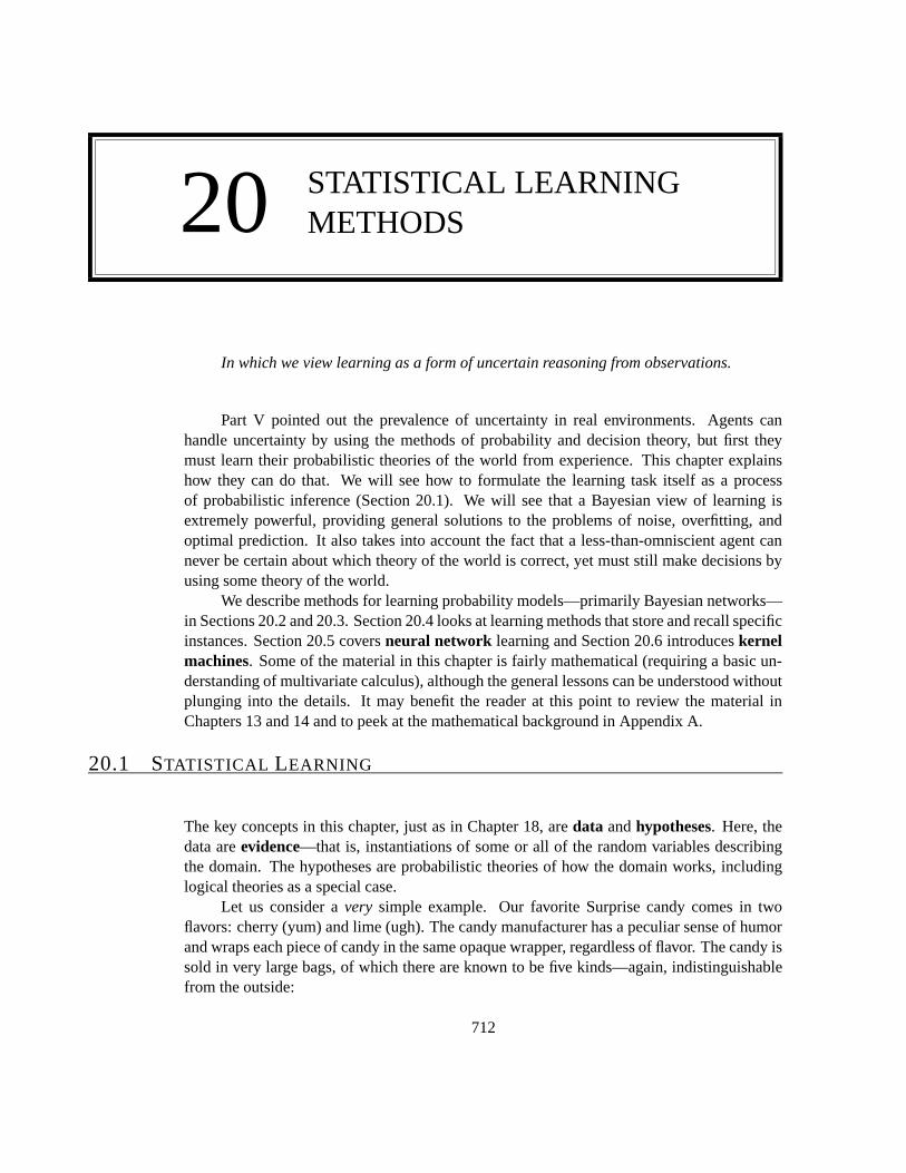
For example, suppose the bag is really an all-lime bag (h5) and the first 10 candies are alllime; then P (d|h3) is 0.510, because half the candies in an h3 bag are lime.2 Figure 20.1(a)shows how the posterior probabilities of the five hypotheses change as the sequence of 10lime candies is observed. Notice that the probabilities start out at their prior values, so h3
is initially the most likely choice and remains so after 1 lime candy is unwrapped. After 2
1 Statistically sophisticated readers will recognize this scenario as a variant of the urn-and-ball setup. We findurns and balls less compelling than candy; furthermore, candy lends itself to other tasks, such as deciding whetherto trade the bag with a friend—see Exercise 20.3.2 We stated earlier that the bags of candy are very large; otherwise, the i.i.d. assumption fails to hold. Technically,it is more correct (but less hygienic) to rewrap each candy after inspection and return it to the bag.
714 Chapter 20. Statistical Learning Methods
0
0.2
0.4
0.6
0.8
1
0 2 4 6 8 10
Post
erio
r pr
obab
ility
of
hypo
thes
is
Number of samples in d
P(h1 | d)P(h2 | d)P(h3 | d)P(h4 | d)P(h5 | d)
0.4
0.5
0.6
0.7
0.8
0.9
1
0 2 4 6 8 10
Prob
abili
ty th
at n
ext c
andy
is li
me
Number of samples in d
(a) (b)
Figure 20.1 (a) Posterior probabilities P (hi|d1, . . . , dN ) from Equation (20.1). The num-ber of observations N ranges from 1 to 10, and each observation is of a lime candy. (b)Bayesian prediction P (dN+1 = lime|d1, . . . , dN ) from Equation (20.2).
lime candies are unwrapped, h4 is most likely; after 3 or more, h5 (the dreaded all-lime bag)is the most likely. After 10 in a row, we are fairly certain of our fate. Figure 20.1(b) showsthe predicted probability that the next candy is lime, based on Equation (20.2). As we wouldexpect, it increases monotonically toward 1.
The example shows that the true hypothesis eventually dominates the Bayesian predic-tion. This is characteristic of Bayesian learning. For any fixed prior that does not rule out thetrue hypothesis, the posterior probability of any false hypothesis will eventually vanish, sim-ply because the probability of generating “uncharacteristic” data indefinitely is vanishinglysmall. (This point is analogous to one made in the discussion of PAC learning in Chapter 18.)More importantly, the Bayesian prediction is optimal, whether the data set be small or large.Given the hypothesis prior, any other prediction will be correct less often.
The optimality of Bayesian learning comes at a price, of course. For real learningproblems, the hypothesis space is usually very large or infinite, as we saw in Chapter 18. Insome cases, the summation in Equation (20.2) (or integration, in the continuous case) can becarried out tractably, but in most cases we must resort to approximate or simplified methods.
A very common approximation—one that is usually adopted in science—is to make pre-dictions based on a single most probable hypothesis—that is, an hi that maximizes P (hi|d).This is often called a maximum a posteriori or MAP (pronounced “em-ay-pee”) hypothe-MAXIMUM A
POSTERIORI
sis. Predictions made according to an MAP hypothesis hMAP are approximately Bayesian tothe extent that P(X|d) ≈ P(X|hMAP). In our candy example, hMAP =h5 after three limecandies in a row, so the MAP learner then predicts that the fourth candy is lime with prob-ability 1.0—a much more dangerous prediction than the Bayesian prediction of 0.8 shownin Figure 20.1. As more data arrive, the MAP and Bayesian predictions become closer, be-cause the competitors to the MAP hypothesis become less and less probable. Although ourexample doesn’t show it, finding MAP hypotheses is often much easier than Bayesian learn-
Section 20.1. Statistical Learning 715
ing, because it requires solving an optimization problem instead of a large summation (orintegration) problem. We will see examples of this later in the chapter.
In both Bayesian learning and MAP learning, the hypothesis prior P (hi) plays an im-portant role. We saw in Chapter 18 that overfitting can occur when the hypothesis spaceis too expressive, so that it contains many hypotheses that fit the data set well. Rather thanplacing an arbitrary limit on the hypotheses to be considered, Bayesian and MAP learningmethods use the prior to penalize complexity. Typically, more complex hypotheses have alower prior probability—in part because there are usually many more complex hypothesesthan simple hypotheses. On the other hand, more complex hypotheses have a greater capac-ity to fit the data. (In the extreme case, a lookup table can reproduce the data exactly withprobability 1.) Hence, the hypothesis prior embodies a trade-off between the complexity of ahypothesis and its degree of fit to the data.
We can see the effect of this trade-off most clearly in the logical case, where H containsonly deterministic hypotheses. In that case, P (d|hi) is 1 if hi is consistent and 0 otherwise.Looking at Equation (20.1), we see that hMAP will then be the simplest logical theory thatis consistent with the data. Therefore, maximum a posteriori learning provides a naturalembodiment of Ockham’s razor.
Another insight into the trade-off between complexity and degree of fit is obtainedby taking the logarithm of Equation (20.1). Choosing hMAP to maximize P (d|hi)P (hi)is equivalent to minimizing
− log2 P (d|hi)− log2 P (hi) .
Using the connection between information encoding and probability that we introduced inChapter 18, we see that the − log2 P (hi) term equals the number of bits required to specifythe hypothesis hi. Furthermore, − log2 P (d|hi) is the additional number of bits requiredto specify the data, given the hypothesis. (To see this, consider that no bits are requiredif the hypothesis predicts the data exactly—as with h5 and the string of lime candies—andlog2 1= 0.) Hence, MAP learning is choosing the hypothesis that provides maximum com-pression of the data. The same task is addressed more directly by the minimum descriptionlength, or MDL, learning method, which attempts to minimize the size of hypothesis and
MINIMUMDESCRIPTIONLENGTH
data encodings rather than work with probabilities.A final simplification is provided by assuming a uniform prior over the space of hy-
potheses. In that case, MAP learning reduces to choosing an hi that maximizes P (d|Hi).This is called a maximum-likelihood (ML) hypothesis, hML. Maximum-likelihood learningMAXIMUM-
LIKELIHOOD
is very common in statistics, a discipline in which many researchers distrust the subjectivenature of hypothesis priors. It is a reasonable approach when there is no reason to prefer onehypothesis over another a priori—for example, when all hypotheses are equally complex. Itprovides a good approximation to Bayesian and MAP learning when the data set is large,because the data swamps the prior distribution over hypotheses, but it has problems (as weshall see) with small data sets.
716 Chapter 20. Statistical Learning Methods
20.2 LEARNING WITH COMPLETE DATA
Our development of statistical learning methods begins with the simplest task: parameterlearning with complete data. A parameter learning task involves finding the numerical pa-PARAMETER
LEARNING
COMPLETE DATA rameters for a probability model whose structure is fixed. For example, we might be interestedin learning the conditional probabilities in a Bayesian network with a given structure. Dataare complete when each data point contains values for every variable in the probability modelbeing learned. Complete data greatly simplify the problem of learning the parameters of acomplex model. We will also look briefly at the problem of learning structure.
Maximum-likelihood parameter learning: Discrete models
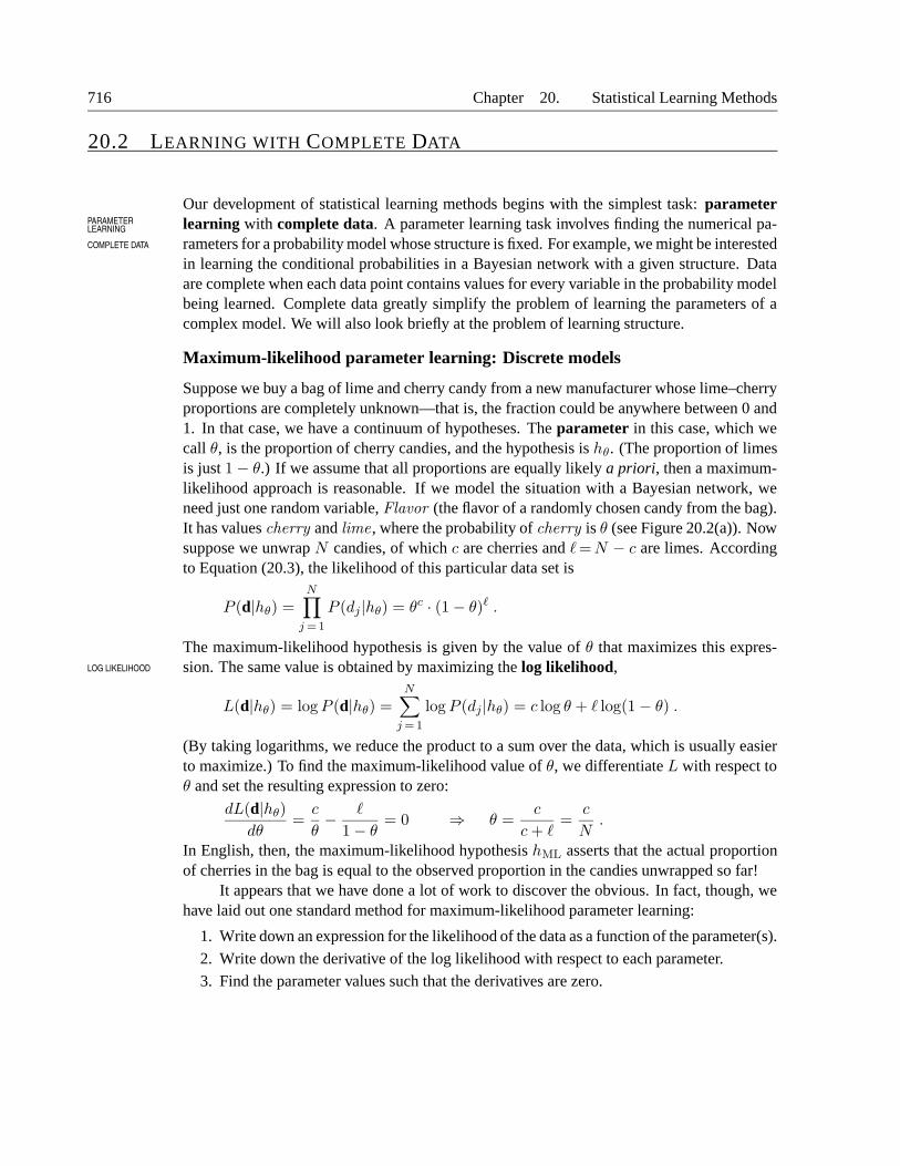
Suppose we buy a bag of lime and cherry candy from a new manufacturer whose lime–cherryproportions are completely unknown—that is, the fraction could be anywhere between 0 and1. In that case, we have a continuum of hypotheses. The parameter in this case, which wecall θ, is the proportion of cherry candies, and the hypothesis is hθ. (The proportion of limesis just 1− θ.) If we assume that all proportions are equally likely a priori, then a maximum-likelihood approach is reasonable. If we model the situation with a Bayesian network, weneed just one random variable, Flavor (the flavor of a randomly chosen candy from the bag).It has values cherry and lime, where the probability of cherry is θ (see Figure 20.2(a)). Nowsuppose we unwrap N candies, of which c are cherries and `= N − c are limes. Accordingto Equation (20.3), the likelihood of this particular data set is
P (d|hθ) =N∏
j =1
P (dj |hθ) = θc · (1− θ)` .
The maximum-likelihood hypothesis is given by the value of θ that maximizes this expres-sion. The same value is obtained by maximizing the log likelihood,LOG LIKELIHOOD
L(d|hθ) = log P (d|hθ) =N∑
j =1
log P (dj|hθ) = c log θ + ` log(1− θ) .
(By taking logarithms, we reduce the product to a sum over the data, which is usually easierto maximize.) To find the maximum-likelihood value of θ, we differentiate L with respect toθ and set the resulting expression to zero:
dL(d|hθ)
dθ=
c
θ− `
1− θ= 0 ⇒ θ =
c
c + `=
c
N.
In English, then, the maximum-likelihood hypothesis hML asserts that the actual proportionof cherries in the bag is equal to the observed proportion in the candies unwrapped so far!
It appears that we have done a lot of work to discover the obvious. In fact, though, wehave laid out one standard method for maximum-likelihood parameter learning:
1. Write down an expression for the likelihood of the data as a function of the parameter(s).
2. Write down the derivative of the log likelihood with respect to each parameter.
3. Find the parameter values such that the derivatives are zero.
Section 20.2. Learning with Complete Data 717
Flavor
P(F=cherry)
(a)
θ
P(F=cherry)
Flavor
Wrapper
(b)
θ
F
cherry
lime
P(W=red | F)
θ1
θ2
Figure 20.2 (a) Bayesian network model for the case of candies with an unknown propor-tion of cherries and limes. (b) Model for the case where the wrapper color depends (proba-bilistically) on the candy flavor.
The trickiest step is usually the last. In our example, it was trivial, but we will see that inmany cases we need to resort to iterative solution algorithms or other numerical optimizationtechniques, as described in Chapter 4. The example also illustrates a significant problemwith maximum-likelihood learning in general: when the data set is small enough that someevents have not yet been observed—for instance, no cherry candies—the maximum likelihoodhypothesis assigns zero probability to those events. Various tricks are used to avoid thisproblem, such as initializing the counts for each event to 1 instead of zero.
Let us look at another example. Suppose this new candy manufacturer wants to give alittle hint to the consumer and uses candy wrappers colored red and green. The Wrapper foreach candy is selected probabilistically, according to some unknown conditional distribution,depending on the flavor. The corresponding probability model is shown in Figure 20.2(b).Notice that it has three parameters: θ, θ1, and θ2. With these parameters, the likelihood ofseeing, say, a cherry candy in a green wrapper can be obtained from the standard semanticsfor Bayesian networks (page 495):
P (Flavor = cherry,Wrapper = green|hθ,θ1,θ2)
= P (Flavor = cherry|hθ,θ1,θ2)P (Wrapper = green|Flavor = cherry, hθ,θ1,θ2)
= θ · (1− θ1) .
Now, we unwrap N candies, of which c are cherries and ` are limes. The wrapper counts areas follows: rc of the cherries have red wrappers and gc have green, while r` of the limes havered and g` have green. The likelihood of the data is given by
P (d|hθ,θ1,θ2) = θc(1− θ)` · θrc1 (1− θ1)
gc · θr`2 (1− θ2)
g` .
This looks pretty horrible, but taking logarithms helps:
L = [c log θ + ` log(1− θ)] + [rc log θ1 + gc log(1− θ1)] + [r` log θ2 + g` log(1− θ2)] .
The benefit of taking logs is clear: the log likelihood is the sum of three terms, each of whichcontains a single parameter. When we take derivatives with respect to each parameter and set
718 Chapter 20. Statistical Learning Methods
them to zero, we get three independent equations, each containing just one parameter:∂L∂θ = c
θ − `1−θ = 0 ⇒ θ = c
c+`∂L∂θ1
= rc
θ1− gc
1−θ1= 0 ⇒ θ1 = rc
rc+gc∂L∂θ2
= r`
θ2− g`
1−θ2= 0 ⇒ θ2 = r`
r`+g`.
The solution for θ is the same as before. The solution for θ1, the probability that a cherrycandy has a red wrapper, is the observed fraction of cherry candies with red wrappers, andsimilarly for θ2.
These results are very comforting, and it is easy to see that they can be extended to anyBayesian network whose conditional probabilities are represented as tables. The most impor-tant point is that, with complete data, the maximum-likelihood parameter learning problemfor a Bayesian network decomposes into separate learning problems, one for each parame-ter.3 The second point is that the parameter values for a variable, given its parents, are just theobserved frequencies of the variable values for each setting of the parent values. As before,we must be careful to avoid zeroes when the data set is small.
Naive Bayes models
Probably the most common Bayesian network model used in machine learning is the naiveBayes model. In this model, the “class” variable C (which is to be predicted) is the rootand the “attribute” variables Xi are the leaves. The model is “naive” because it assumes thatthe attributes are conditionally independent of each other, given the class. (The model inFigure 20.2(b) is a naive Bayes model with just one attribute.) Assuming Boolean variables,the parameters are
θ = P (C = true), θi1 =P (Xi = true|C = true), θi2 =P (Xi = true|C = false).
The maximum-likelihood parameter values are found in exactly the same way as for Fig-ure 20.2(b). Once the model has been trained in this way, it can be used to classify new exam-ples for which the class variable C is unobserved. With observed attribute values x1, . . . , xn,the probability of each class is given by
P(C|x1, . . . , xn) = α P(C)∏
i
P(xi|C) .
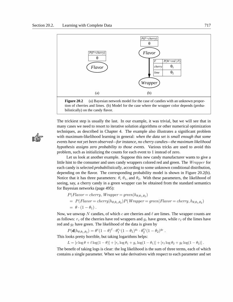
A deterministic prediction can be obtained by choosing the most likely class. Figure 20.3shows the learning curve for this method when it is applied to the restaurant problem fromChapter 18. The method learns fairly well but not as well as decision-tree learning; this ispresumably because the true hypothesis—which is a decision tree—is not representable ex-actly using a naive Bayes model. Naive Bayes learning turns out to do surprisingly well in awide range of applications; the boosted version (Exercise 20.5) is one of the most effectivegeneral-purpose learning algorithms. Naive Bayes learning scales well to very large prob-lems: with n Boolean attributes, there are just 2n + 1 parameters, and no search is requiredto find hML, the maximum-likelihood naive Bayes hypothesis. Finally, naive Bayes learninghas no difficulty with noisy data and can give probabilistic predictions when appropriate.
3 See Exercise 20.7 for the nontabulated case, where each parameter affects several conditional probabilities.
Section 20.2. Learning with Complete Data 719
0.4
0.5
0.6
0.7
0.8
0.9
1
0 20 40 60 80 100
Prop
ortio
n co
rrec
t on
test
set
Training set size
Decision treeNaive Bayes
Figure 20.3 The learning curve for naive Bayes learning applied to the restaurant problemfrom Chapter 18; the learning curve for decision-tree learning is shown for comparison.
Maximum-likelihood parameter learning: Continuous models
Continuous probability models such as the linear-Gaussian model were introduced in Sec-tion 14.3. Because continuous variables are ubiquitous in real-world applications, it is im-portant to know how to learn continuous models from data. The principles for maximum-likelihood learning are identical to those of the discrete case.
Let us begin with a very simple case: learning the parameters of a Gaussian densityfunction on a single variable. That is, the data are generated as follows:
P (x) =1√2πσ
e−(x−µ)2
2σ2 .
The parameters of this model are the mean µ and the standard deviation σ. (Notice that thenormalizing “constant” depends on σ, so we cannot ignore it.) Let the observed values bex1, . . . , xN . Then the log likelihood is
L =N∑
j =1
log1√2πσ
e−(xj−µ)2
2σ2 = N(− log√
2π − log σ)−N∑
j =1
(xj − µ)2
2σ2.
Setting the derivatives to zero as usual, we obtain
∂L∂µ = − 1
σ2
∑Nj=1(xj − µ) = 0 ⇒ µ =
∑
jxj
N
∂L∂σ = −N
σ + 1σ3
∑Nj=1(xj − µ)2 = 0 ⇒ σ =
√
∑
j(xj−µ)2
N .(20.4)
That is, the maximum-likelihood value of the mean is the sample average and the maximum-likelihood value of the standard deviation is the square root of the sample variance. Again,these are comforting results that confirm “commonsense” practice.
Now consider a linear Gaussian model with one continuous parent X and a continuouschild Y . As explained on page 502, Y has a Gaussian distribution whose mean dependslinearly on the value of X and whose standard deviation is fixed. To learn the conditional
720 Chapter 20. Statistical Learning Methods
0 0.2 0.4 0.6 0.8 1x 00.2
0.40.6
0.81
y0
0.51
1.52
2.53
3.54P(y |x)
0
0.2
0.4
0.6
0.8
1
0 0.1 0.2 0.3 0.4 0.5 0.6 0.7 0.8 0.9 1
y
x
(a) (b)
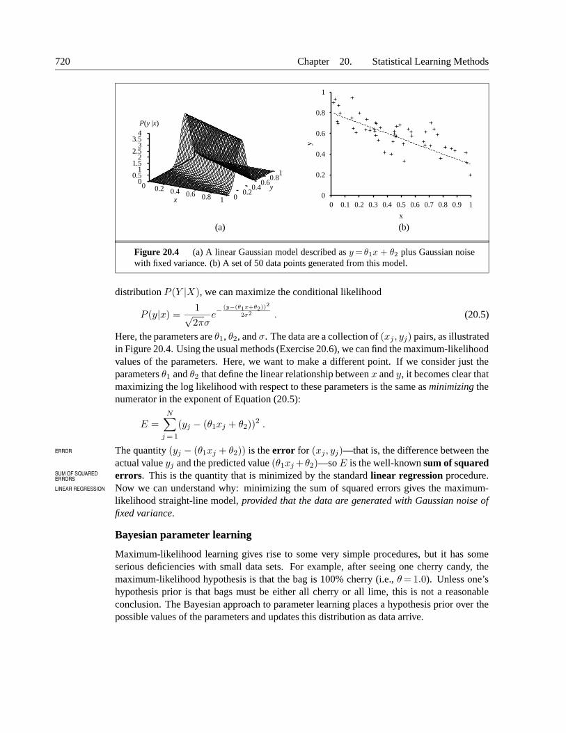
Figure 20.4 (a) A linear Gaussian model described as y = θ1x + θ2 plus Gaussian noisewith fixed variance. (b) A set of 50 data points generated from this model.
distribution P (Y |X), we can maximize the conditional likelihood
P (y|x) =1√2πσ
e−(y−(θ1x+θ2))2
2σ2 . (20.5)
Here, the parameters are θ1, θ2, and σ. The data are a collection of (xj , yj) pairs, as illustratedin Figure 20.4. Using the usual methods (Exercise 20.6), we can find the maximum-likelihoodvalues of the parameters. Here, we want to make a different point. If we consider just theparameters θ1 and θ2 that define the linear relationship between x and y, it becomes clear thatmaximizing the log likelihood with respect to these parameters is the same as minimizing thenumerator in the exponent of Equation (20.5):
E =N∑
j =1
(yj − (θ1xj + θ2))2 .
The quantity (yj − (θ1xj + θ2)) is the error for (xj, yj)—that is, the difference between theERROR
actual value yj and the predicted value (θ1xj +θ2)—so E is the well-known sum of squarederrors. This is the quantity that is minimized by the standard linear regression procedure.SUM OF SQUARED
ERRORS
LINEAR REGRESSION Now we can understand why: minimizing the sum of squared errors gives the maximum-likelihood straight-line model, provided that the data are generated with Gaussian noise offixed variance.
Bayesian parameter learning
Maximum-likelihood learning gives rise to some very simple procedures, but it has someserious deficiencies with small data sets. For example, after seeing one cherry candy, themaximum-likelihood hypothesis is that the bag is 100% cherry (i.e., θ = 1.0). Unless one’shypothesis prior is that bags must be either all cherry or all lime, this is not a reasonableconclusion. The Bayesian approach to parameter learning places a hypothesis prior over thepossible values of the parameters and updates this distribution as data arrive.
Section 20.2. Learning with Complete Data 721
0
0.5
1
1.5
2
2.5
0 0.2 0.4 0.6 0.8 1
P(Θ
= θ
)
Parameter θ
[1,1]
[2,2]
[5,5]
0
1
2
3
4
5
6
0 0.2 0.4 0.6 0.8 1
P(Θ
= θ
)
Parameter θ
[3,1]
[6,2]
[30,10]
(a) (b)
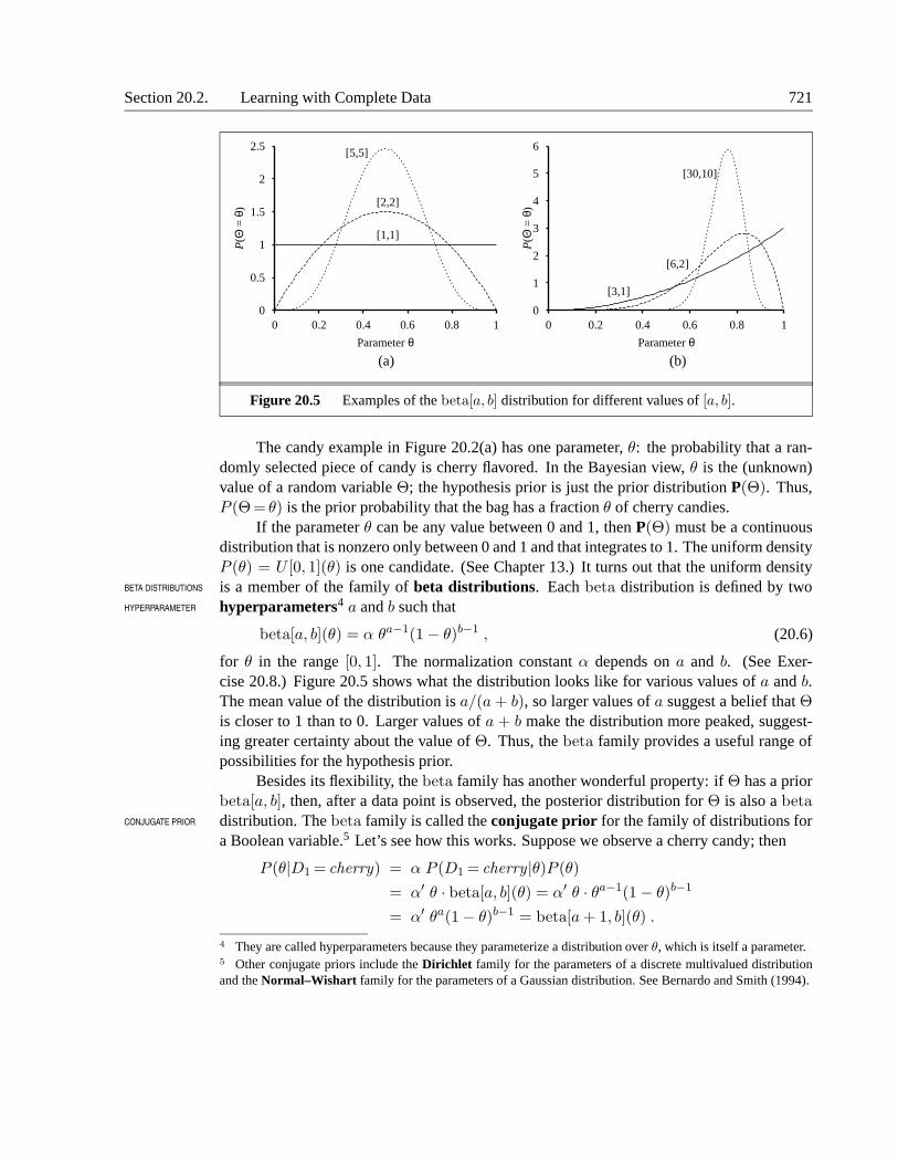
Figure 20.5 Examples of the beta[a, b] distribution for different values of [a, b].
The candy example in Figure 20.2(a) has one parameter, θ: the probability that a ran-domly selected piece of candy is cherry flavored. In the Bayesian view, θ is the (unknown)value of a random variable Θ; the hypothesis prior is just the prior distribution P(Θ). Thus,P (Θ= θ) is the prior probability that the bag has a fraction θ of cherry candies.
If the parameter θ can be any value between 0 and 1, then P(Θ) must be a continuousdistribution that is nonzero only between 0 and 1 and that integrates to 1. The uniform densityP (θ) = U [0, 1](θ) is one candidate. (See Chapter 13.) It turns out that the uniform densityis a member of the family of beta distributions. Each beta distribution is defined by twoBETA DISTRIBUTIONS
hyperparameters4 a and b such thatHYPERPARAMETER
beta[a, b](θ) = α θa−1(1− θ)b−1 , (20.6)
for θ in the range [0, 1]. The normalization constant α depends on a and b. (See Exer-cise 20.8.) Figure 20.5 shows what the distribution looks like for various values of a and b.The mean value of the distribution is a/(a + b), so larger values of a suggest a belief that Θis closer to 1 than to 0. Larger values of a + b make the distribution more peaked, suggest-ing greater certainty about the value of Θ. Thus, the beta family provides a useful range ofpossibilities for the hypothesis prior.
Besides its flexibility, the beta family has another wonderful property: if Θ has a priorbeta[a, b], then, after a data point is observed, the posterior distribution for Θ is also a betadistribution. The beta family is called the conjugate prior for the family of distributions forCONJUGATE PRIOR
a Boolean variable.5 Let’s see how this works. Suppose we observe a cherry candy; then
P (θ|D1 = cherry) = α P (D1 = cherry|θ)P (θ)
= α′ θ · beta[a, b](θ) = α′ θ · θa−1(1− θ)b−1
= α′ θa(1− θ)b−1 = beta[a + 1, b](θ) .
4 They are called hyperparameters because they parameterize a distribution over θ, which is itself a parameter.5 Other conjugate priors include the Dirichlet family for the parameters of a discrete multivalued distributionand the Normal–Wishart family for the parameters of a Gaussian distribution. See Bernardo and Smith (1994).
722 Chapter 20. Statistical Learning Methods
Thus, after seeing a cherry candy, we simply increment the a parameter to get the posterior;similarly, after seeing a lime candy, we increment the b parameter. Thus, we can view the aand b hyperparameters as virtual counts, in the sense that a prior beta[a, b] behaves exactlyVIRTUAL COUNTS
as if we had started out with a uniform prior beta[1, 1] and seen a − 1 actual cherry candiesand b− 1 actual lime candies.
By examining a sequence of beta distributions for increasing values of a and b, keepingthe proportions fixed, we can see vividly how the posterior distribution over the parameter Θchanges as data arrive. For example, suppose the actual bag of candy is 75% cherry. Fig-ure 20.5(b) shows the sequence beta[3, 1], beta[6, 2], beta[30, 10]. Clearly, the distributionis converging to a narrow peak around the true value of Θ. For large data sets, then, Bayesianlearning (at least in this case) converges to give the same results as maximum-likelihoodlearning.
The network in Figure 20.2(b) has three parameters, θ, θ1, and θ2, where θ1 is theprobability of a red wrapper on a cherry candy and θ2 is the probability of a red wrapper on alime candy. The Bayesian hypothesis prior must cover all three parameters—that is, we needto specify P(Θ,Θ1,Θ2). Usually, we assume parameter independence:PARAMETER
INDEPENDENCE
P(Θ,Θ1,Θ2) = P(Θ)P(Θ1)P(Θ2) .
With this assumption, each parameter can have its own beta distribution that is updated sep-arately as data arrive.
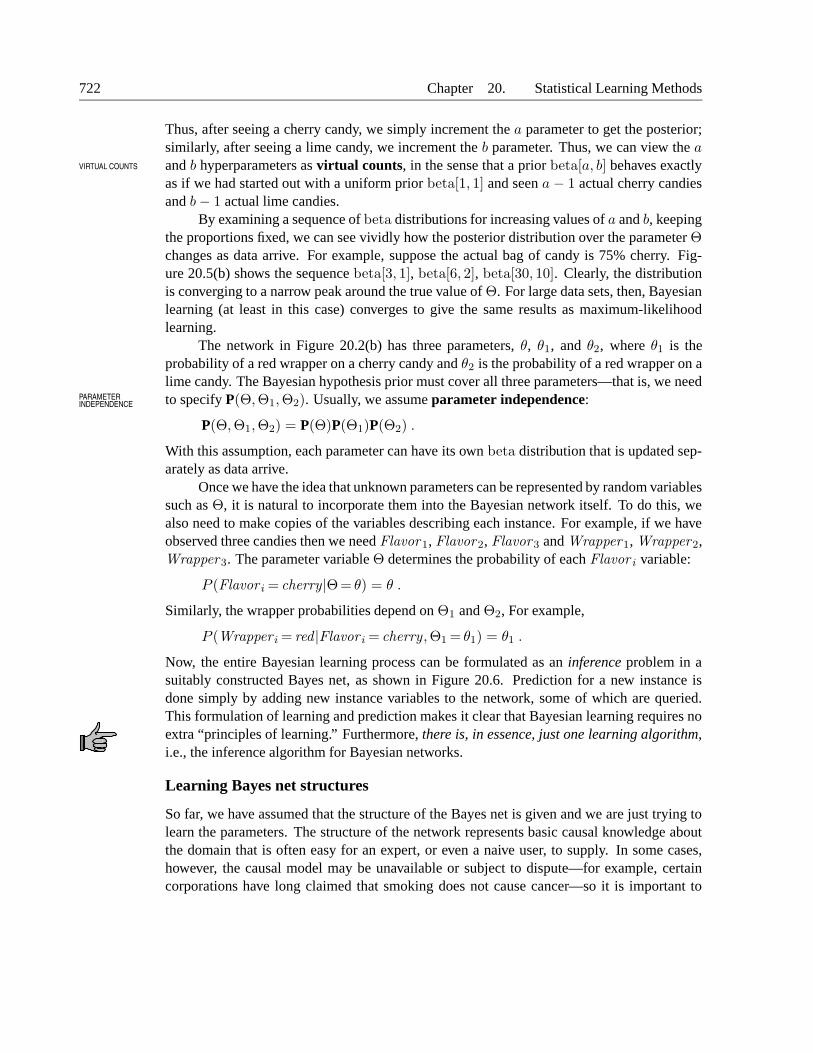
Once we have the idea that unknown parameters can be represented by random variablessuch as Θ, it is natural to incorporate them into the Bayesian network itself. To do this, wealso need to make copies of the variables describing each instance. For example, if we haveobserved three candies then we need Flavor 1, Flavor2, Flavor3 and Wrapper1, Wrapper2,Wrapper3. The parameter variable Θ determines the probability of each Flavor i variable:
P (Flavor i = cherry|Θ= θ) = θ .
Similarly, the wrapper probabilities depend on Θ1 and Θ2, For example,
P (Wrapper i = red |Flavor i = cherry,Θ1 = θ1) = θ1 .
Now, the entire Bayesian learning process can be formulated as an inference problem in asuitably constructed Bayes net, as shown in Figure 20.6. Prediction for a new instance isdone simply by adding new instance variables to the network, some of which are queried.This formulation of learning and prediction makes it clear that Bayesian learning requires noextra “principles of learning.” Furthermore, there is, in essence, just one learning algorithm,i.e., the inference algorithm for Bayesian networks.
Learning Bayes net structures
So far, we have assumed that the structure of the Bayes net is given and we are just trying tolearn the parameters. The structure of the network represents basic causal knowledge aboutthe domain that is often easy for an expert, or even a naive user, to supply. In some cases,however, the causal model may be unavailable or subject to dispute—for example, certaincorporations have long claimed that smoking does not cause cancer—so it is important to
Section 20.2. Learning with Complete Data 723
Flavor1
Wrapper1
Flavor2
Wrapper2
Flavor3
Wrapper3
Θ
Θ1 Θ2
Figure 20.6 A Bayesian network that corresponds to a Bayesian learning process. Poste-rior distributions for the parameter variables Θ, Θ1, and Θ2 can be inferred from their priordistributions and the evidence in the Flavor i and Wrapper i variables.
understand how the structure of a Bayes net can be learned from data. At present, structurallearning algorithms are in their infancy, so we will give only a brief sketch of the main ideas.
The most obvious approach is to search for a good model. We can start with a modelcontaining no links and begin adding parents for each node, fitting the parameters with themethods we have just covered and measuring the accuracy of the resulting model. Alterna-tively, we can start with an initial guess at the structure and use hill-climbing or simulatedannealing search to make modifications, retuning the parameters after each change in thestructure. Modifications can include reversing, adding, or deleting arcs. We must not in-troduce cycles in the process, so many algorithms assume that an ordering is given for thevariables, and that a node can have parents only among those nodes that come earlier in theordering (just as in the construction process Chapter 14). For full generality, we also need tosearch over possible orderings.
There are two alternative methods for deciding when a good structure has been found.The first is to test whether the conditional independence assertions implicit in the structure areactually satisfied in the data. For example, the use of a naive Bayes model for the restaurantproblem assumes that
P(Fri/Sat ,Bar |WillWait) = P(Fri/Sat |WillWait)P(Bar |WillWait)
and we can check in the data that the same equation holds between the corresponding condi-tional frequencies. Now, even if the structure describes the true causal nature of the domain,statistical fluctuations in the data set mean that the equation will never be satisfied exactly,so we need to perform a suitable statistical test to see if there is sufficient evidence that theindependence hypothesis is violated. The complexity of the resulting network will depend
724 Chapter 20. Statistical Learning Methods
on the threshold used for this test—the stricter the independence test, the more links will beadded and the greater the danger of overfitting.
An approach more consistent with the ideas in this chapter is to the degree to whichthe proposed model explains the data (in a probabilistic sense). We must be careful how wemeasure this, however. If we just try to find the maximum-likelihood hypothesis, we will endup with a fully connected network, because adding more parents to a node cannot decreasethe likelihood (Exercise 20.9). We are forced to penalize model complexity in some way.The MAP (or MDL) approach simply subtracts a penalty from the likelihood of each structure(after parameter tuning) before comparing different structures. The Bayesian approach placesa joint prior over structures and parameters. There are usually far too many structures tosum over (superexponential in the number of variables), so most practitioners use MCMC tosample over structures.
Penalizing complexity (whether by MAP or Bayesian methods) introduces an importantconnection between the optimal structure and the nature of the representation for the condi-tional distributions in the network. With tabular distributions, the complexity penalty for anode’s distribution grows exponentially with the number of parents, but with, say, noisy-ORdistributions, it grows only linearly. This means that learning with noisy-OR (or other com-pactly parameterized) models tends to produce learned structures with more parents than doeslearning with tabular distributions.
20.3 LEARNING WITH HIDDEN VARIABLES: THE EM ALGORITHM
The preceding section dealt with the fully observable case. Many real-world problems havehidden variables (sometimes called latent variables) which are not observable in the dataLATENT VARIABLES
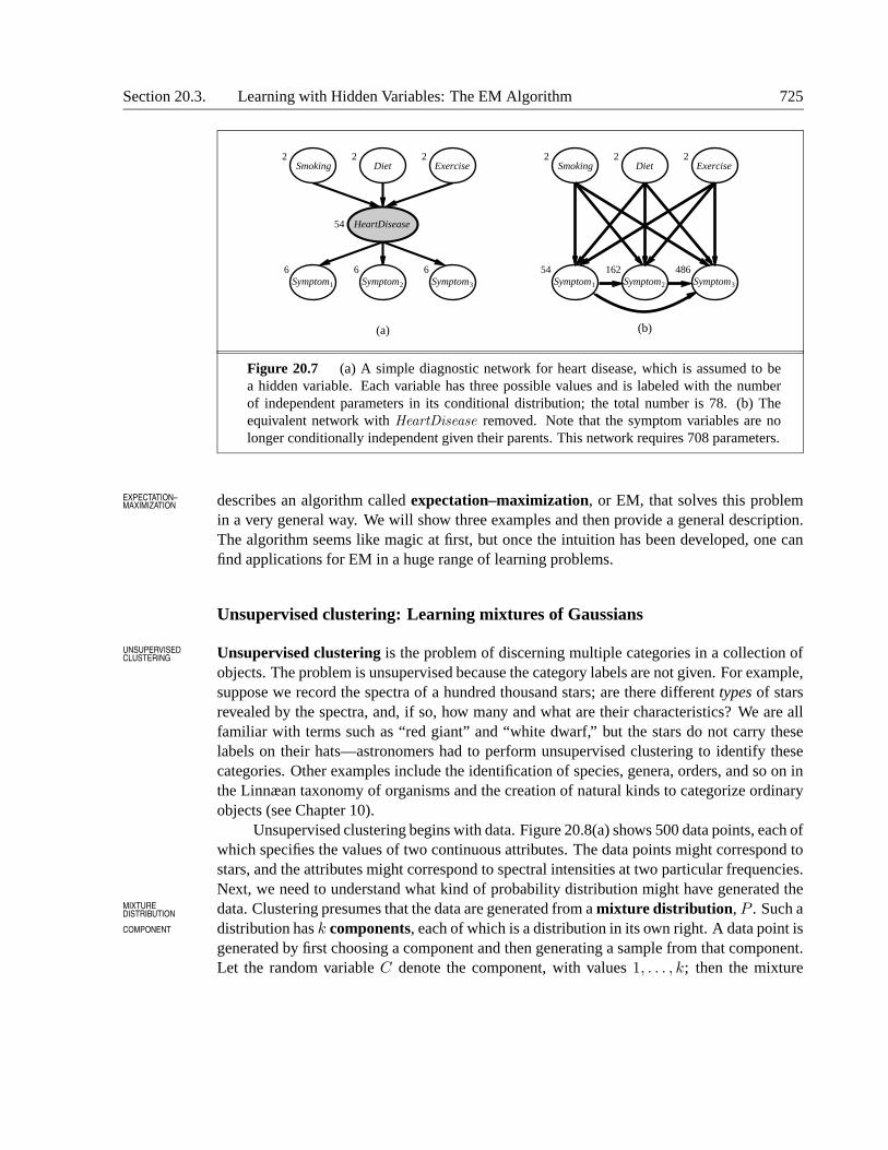
that are available for learning. For example, medical records often include the observedsymptoms, the treatment applied, and perhaps the outcome of the treatment, but they sel-dom contain a direct observation of the disease itself!6 One might ask, “If the disease isnot observed, why not construct a model without it?” The answer appears in Figure 20.7,which shows a small, fictitious diagnostic model for heart disease. There are three observ-able predisposing factors and three observable symptoms (which are too depressing to name).Assume that each variable has three possible values (e.g., none , moderate, and severe). Re-moving the hidden variable from the network in (a) yields the network in (b); the total numberof parameters increases from 78 to 708. Thus, latent variables can dramatically reduce thenumber of parameters required to specify a Bayesian network. This, in turn, can dramaticallyreduce the amount of data needed to learn the parameters.
Hidden variables are important, but they do complicate the learning problem. In Fig-ure 20.7(a), for example, it is not obvious how to learn the conditional distribution forHeartDisease, given its parents, because we do not know the value of HeartDisease in eachcase; the same problem arises in learning the distributions for the symptoms. This section
6 Some records contain the diagnosis suggested by the physician, but this is a causal consequence of the symp-toms, which are in turn caused by the disease.
Section 20.3. Learning with Hidden Variables: The EM Algorithm 725
Smoking Diet Exercise
Symptom1 Symptom2 Symptom3
(a) (b)
HeartDisease
Smoking Diet Exercise
Symptom1 Symptom2 Symptom3
2 2 2
54
6 6 6
2 2 2
54 162 486
Figure 20.7 (a) A simple diagnostic network for heart disease, which is assumed to bea hidden variable. Each variable has three possible values and is labeled with the numberof independent parameters in its conditional distribution; the total number is 78. (b) Theequivalent network with HeartDisease removed. Note that the symptom variables are nolonger conditionally independent given their parents. This network requires 708 parameters.
describes an algorithm called expectation–maximization, or EM, that solves this problemEXPECTATION–MAXIMIZATION
in a very general way. We will show three examples and then provide a general description.The algorithm seems like magic at first, but once the intuition has been developed, one canfind applications for EM in a huge range of learning problems.
Unsupervised clustering: Learning mixtures of Gaussians
Unsupervised clustering is the problem of discerning multiple categories in a collection ofUNSUPERVISEDCLUSTERING
objects. The problem is unsupervised because the category labels are not given. For example,suppose we record the spectra of a hundred thousand stars; are there different types of starsrevealed by the spectra, and, if so, how many and what are their characteristics? We are allfamiliar with terms such as “red giant” and “white dwarf,” but the stars do not carry theselabels on their hats—astronomers had to perform unsupervised clustering to identify thesecategories. Other examples include the identification of species, genera, orders, and so on inthe Linnæan taxonomy of organisms and the creation of natural kinds to categorize ordinaryobjects (see Chapter 10).
Unsupervised clustering begins with data. Figure 20.8(a) shows 500 data points, each ofwhich specifies the values of two continuous attributes. The data points might correspond tostars, and the attributes might correspond to spectral intensities at two particular frequencies.Next, we need to understand what kind of probability distribution might have generated thedata. Clustering presumes that the data are generated from a mixture distribution, P . Such aMIXTURE
DISTRIBUTION
distribution has k components, each of which is a distribution in its own right. A data point isCOMPONENT
generated by first choosing a component and then generating a sample from that component.Let the random variable C denote the component, with values 1, . . . , k; then the mixture
726 Chapter 20. Statistical Learning Methods
0
0.2
0.4
0.6
0.8
1
0 0.2 0.4 0.6 0.8 10
0.2
0.4
0.6
0.8
1
0 0.2 0.4 0.6 0.8 10
0.2
0.4
0.6
0.8
1
0 0.2 0.4 0.6 0.8 1(a) (b) (c)
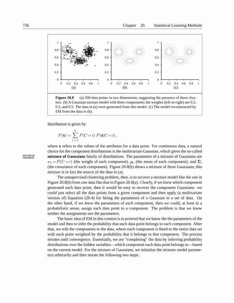
Figure 20.8 (a) 500 data points in two dimensions, suggesting the presence of three clus-ters. (b) A Gaussian mixture model with three components; the weights (left-to-right) are 0.2,0.3, and 0.5. The data in (a) were generated from this model. (c) The model reconstructed byEM from the data in (b).
distribution is given by
P (x) =k∑
i =1
P (C = i) P (x|C = i) ,
where x refers to the values of the attributes for a data point. For continuous data, a naturalchoice for the component distributions is the multivariate Gaussian, which gives the so-calledmixture of Gaussians family of distributions. The parameters of a mixture of Gaussians areMIXTURE OF
GAUSSIANS
wi = P (C = i) (the weight of each component), µi (the mean of each component), and Σi
(the covariance of each component). Figure 20.8(b) shows a mixture of three Gaussians; thismixture is in fact the source of the data in (a).
The unsupervised clustering problem, then, is to recover a mixture model like the one inFigure 20.8(b) from raw data like that in Figure 20.8(a). Clearly, if we knew which componentgenerated each data point, then it would be easy to recover the component Gaussians: wecould just select all the data points from a given component and then apply (a multivariateversion of) Equation (20.4) for fitting the parameters of a Gaussian to a set of data. Onthe other hand, if we knew the parameters of each component, then we could, at least in aprobabilistic sense, assign each data point to a component. The problem is that we knowneither the assignments nor the parameters.
The basic idea of EM in this context is to pretend that we know the the parameters of themodel and then to infer the probability that each data point belongs to each component. Afterthat, we refit the components to the data, where each component is fitted to the entire data setwith each point weighted by the probability that it belongs to that component. The processiterates until convergence. Essentially, we are “completing” the data by inferring probabilitydistributions over the hidden variables—which component each data point belongs to—basedon the current model. For the mixture of Gaussians, we initialize the mixture model parame-ters arbitrarily and then iterate the following two steps:
Section 20.3. Learning with Hidden Variables: The EM Algorithm 727
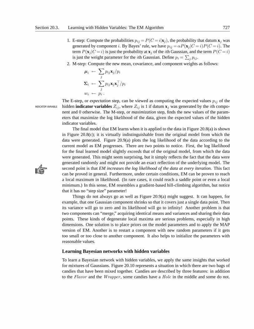
1. E-step: Compute the probabilities pij = P (C = i|xj), the probability that datum xj wasgenerated by component i. By Bayes’ rule, we have pij =αP (xj |C = i)P (C = i). Theterm P (xj |C = i) is just the probability at xj of the ith Gaussian, and the term P (C = i)is just the weight parameter for the ith Gaussian. Define pi =
∑
j pij .
2. M-step: Compute the new mean, covariance, and component weights as follows:
µi ←∑
j
pijxj/pi
Σi ←∑
j
pijxjx>j /pi
wi ← pi .
The E-step, or expectation step, can be viewed as computing the expected values pij of thehidden indicator variables Zij , where Zij is 1 if datum xj was generated by the ith compo-INDICATOR VARIABLE
nent and 0 otherwise. The M-step, or maximization step, finds the new values of the param-eters that maximize the log likelihood of the data, given the expected values of the hiddenindicator variables.
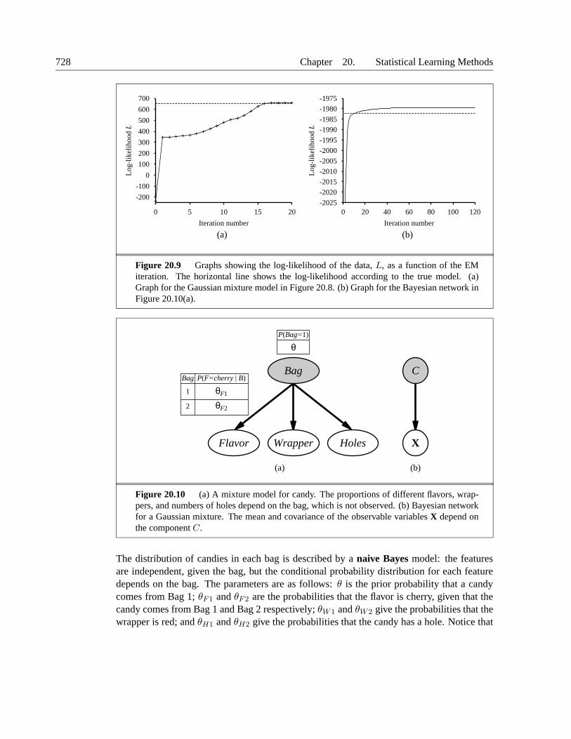
The final model that EM learns when it is applied to the data in Figure 20.8(a) is shownin Figure 20.8(c); it is virtually indistinguishable from the original model from which thedata were generated. Figure 20.9(a) plots the log likelihood of the data according to thecurrent model as EM progresses. There are two points to notice. First, the log likelihoodfor the final learned model slightly exceeds that of the original model, from which the datawere generated. This might seem surprising, but it simply reflects the fact that the data weregenerated randomly and might not provide an exact reflection of the underlying model. Thesecond point is that EM increases the log likelihood of the data at every iteration. This factcan be proved in general. Furthermore, under certain conditions, EM can be proven to reacha local maximum in likelihood. (In rare cases, it could reach a saddle point or even a localminimum.) In this sense, EM resembles a gradient-based hill-climbing algorithm, but noticethat it has no “step size” parameter!
Things do not always go as well as Figure 20.9(a) might suggest. It can happen, forexample, that one Gaussian component shrinks so that it covers just a single data point. Thenits variance will go to zero and its likelihood will go to infinity! Another problem is thattwo components can “merge,” acquiring identical means and variances and sharing their datapoints. These kinds of degenerate local maxima are serious problems, especially in highdimensions. One solution is to place priors on the model parameters and to apply the MAPversion of EM. Another is to restart a component with new random parameters if it getstoo small or too close to another component. It also helps to initialize the parameters withreasonable values.
Learning Bayesian networks with hidden variables
To learn a Bayesian network with hidden variables, we apply the same insights that workedfor mixtures of Gaussians. Figure 20.10 represents a situation in which there are two bags ofcandies that have been mixed together. Candies are described by three features: in additionto the Flavor and the Wrapper , some candies have a Hole in the middle and some do not.
728 Chapter 20. Statistical Learning Methods
-200
-100
0
100
200
300
400
500
600
700
0 5 10 15 20
Log
-lik
elih
ood
L
Iteration number
-2025-2020
-2015-2010
-2005-2000-1995
-1990-1985
-1980-1975
0 20 40 60 80 100 120
Log
-lik
elih
ood
L
Iteration number
(a) (b)
Figure 20.9 Graphs showing the log-likelihood of the data, L, as a function of the EMiteration. The horizontal line shows the log-likelihood according to the true model. (a)Graph for the Gaussian mixture model in Figure 20.8. (b) Graph for the Bayesian network inFigure 20.10(a).
(a) (b)
C
X Holes
Bag
P(Bag=1)
θ
Wrapper Flavor
Bag
1
2
P(F=cherry | B)
θF2
θF1
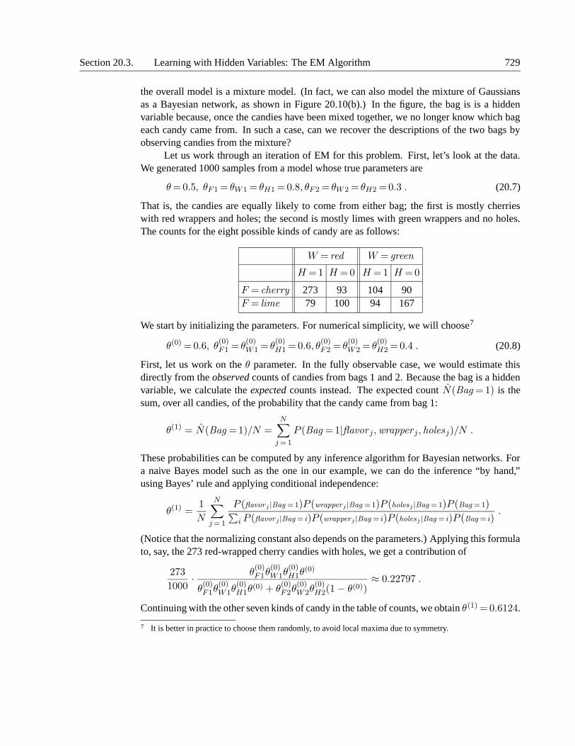
Figure 20.10 (a) A mixture model for candy. The proportions of different flavors, wrap-pers, and numbers of holes depend on the bag, which is not observed. (b) Bayesian networkfor a Gaussian mixture. The mean and covariance of the observable variables X depend onthe component C.
The distribution of candies in each bag is described by a naive Bayes model: the featuresare independent, given the bag, but the conditional probability distribution for each featuredepends on the bag. The parameters are as follows: θ is the prior probability that a candycomes from Bag 1; θF1 and θF2 are the probabilities that the flavor is cherry, given that thecandy comes from Bag 1 and Bag 2 respectively; θW1 and θW2 give the probabilities that thewrapper is red; and θH1 and θH2 give the probabilities that the candy has a hole. Notice that
Section 20.3. Learning with Hidden Variables: The EM Algorithm 729
the overall model is a mixture model. (In fact, we can also model the mixture of Gaussiansas a Bayesian network, as shown in Figure 20.10(b).) In the figure, the bag is is a hiddenvariable because, once the candies have been mixed together, we no longer know which bageach candy came from. In such a case, can we recover the descriptions of the two bags byobserving candies from the mixture?
Let us work through an iteration of EM for this problem. First, let’s look at the data.We generated 1000 samples from a model whose true parameters are
θ = 0.5, θF1 = θW1 = θH1 = 0.8, θF2 = θW2 = θH2 = 0.3 . (20.7)
That is, the candies are equally likely to come from either bag; the first is mostly cherrieswith red wrappers and holes; the second is mostly limes with green wrappers and no holes.The counts for the eight possible kinds of candy are as follows:
W = red W = green
H = 1 H = 0 H = 1 H = 0
F = cherry 273 93 104 90F = lime 79 100 94 167
We start by initializing the parameters. For numerical simplicity, we will choose7
θ(0) = 0.6, θ(0)F1 = θ
(0)W1 = θ
(0)H1 = 0.6, θ
(0)F2 = θ
(0)W2 = θ
(0)H2 =0.4 . (20.8)
First, let us work on the θ parameter. In the fully observable case, we would estimate thisdirectly from the observed counts of candies from bags 1 and 2. Because the bag is a hiddenvariable, we calculate the expected counts instead. The expected count N(Bag = 1) is thesum, over all candies, of the probability that the candy came from bag 1:
θ(1) = N(Bag =1)/N =N∑
j = 1
P (Bag = 1|flavor j ,wrapper j , holesj)/N .
These probabilities can be computed by any inference algorithm for Bayesian networks. Fora naive Bayes model such as the one in our example, we can do the inference “by hand,”using Bayes’ rule and applying conditional independence:
θ(1) =1
N
N∑
j = 1
P (flavorj |Bag =1)P (wrapperj |Bag =1)P (holesj |Bag =1)P (Bag = 1)∑
i P (flavorj |Bag = i)P (wrapperj |Bag = i)P (holesj |Bag = i)P (Bag = i).
(Notice that the normalizing constant also depends on the parameters.) Applying this formulato, say, the 273 red-wrapped cherry candies with holes, we get a contribution of
273
1000· θ
(0)F1θ
(0)W1θ
(0)H1θ
(0)
θ(0)F1θ
(0)W1θ
(0)H1θ
(0) + θ(0)F2θ
(0)W2θ
(0)H2(1− θ(0))
≈ 0.22797 .
Continuing with the other seven kinds of candy in the table of counts, we obtain θ(1) =0.6124.
7 It is better in practice to choose them randomly, to avoid local maxima due to symmetry.
730 Chapter 20. Statistical Learning Methods
0.3 f 0.7 t
P(R ) 1 R 0
0.7 P(R 0 )
0.2 f 0.9 t
P(U ) 1 R 1
Umbrella 1
Rain 0 Rain 1 Rain0
0.7 P(R 0 )
0.2 f 0.9 t
P(U ) 1 R 1
Umbrella1
ft
R
0.30.7
P(R )10
Rain1
Umbrella2
ft
R
0.30.7
P(R )21
Rain2
Umbrella3
ft
R
0.30.7
P(R )32
Rain3
Umbrella4
ft
R
0.30.7
P(R )43
Rain4
0.2f0.9t
P(U )2R2
0.2f0.9t
P(U )3R3
0.2f0.9t
P(U )4R4
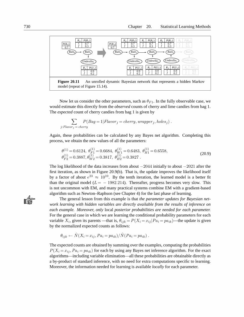
Figure 20.11 An unrolled dynamic Bayesian network that represents a hidden Markovmodel (repeat of Figure 15.14).
Now let us consider the other parameters, such as θF1. In the fully observable case, wewould estimate this directly from the observed counts of cherry and lime candies from bag 1.The expected count of cherry candies from bag 1 is given by
∑
j:Flavorj = cherry
P (Bag = 1|Flavor j = cherry,wrapper j , holesj) .
Again, these probabilities can be calculated by any Bayes net algorithm. Completing thisprocess, we obtain the new values of all the parameters:
θ(1) =0.6124, θ(1)F1 = 0.6684, θ
(1)W1 = 0.6483, θ
(1)H1 = 0.6558,
θ(1)F2 =0.3887, θ
(1)W2 =0.3817, θ
(1)H2 = 0.3827 .
(20.9)
The log likelihood of the data increases from about −2044 initially to about −2021 after thefirst iteration, as shown in Figure 20.9(b). That is, the update improves the likelihood itselfby a factor of about e23 ≈ 1010. By the tenth iteration, the learned model is a better fitthan the original model (L= − 1982.214). Thereafter, progress becomes very slow. Thisis not uncommon with EM, and many practical systems combine EM with a gradient-basedalgorithm such as Newton–Raphson (see Chapter 4) for the last phase of learning.
The general lesson from this example is that the parameter updates for Bayesian net-work learning with hidden variables are directly available from the results of inference oneach example. Moreover, only local posterior probabilities are needed for each parameter.For the general case in which we are learning the conditional probability parameters for eachvariable Xi, given its parents —that is, θijk =P (Xi = xij |Pai = paik)—the update is givenby the normalized expected counts as follows:
θijk ← N(Xi =xij ,Pai = paik)/N(Pai = paik) .
The expected counts are obtained by summing over the examples, computing the probabilitiesP (Xi = xij ,Pai = paik) for each by using any Bayes net inference algorithm. For the exactalgorithms—including variable elimination—all these probabilities are obtainable directly asa by-product of standard inference, with no need for extra computations specific to learning.Moreover, the information needed for learning is available locally for each parameter.
Section 20.3. Learning with Hidden Variables: The EM Algorithm 731
Learning hidden Markov models
Our final application of EM involves learning the transition probabilities in hidden Markovmodels (HMMs). Recall from Chapter 15 that a hidden Markov model can be represented bya dynamic Bayes net with a single discrete state variable, as illustrated in Figure 20.11. Eachdata point consists of an observation sequence of finite length, so the problem is to learn thetransition probabilities from a set of observation sequences (or possibly from just one longsequence).
We have already worked out how to learn Bayes nets, but there is one complication:in Bayes nets, each parameter is distinct; in a hidden Markov model, on the other hand, theindividual transition probabilities from state i to state j at time t, θijt =P (Xt+1 = j|Xt = i),are repeated across time—that is, θijt = θij for all t. To estimate the transition probabilityfrom state i to state j, we simply calculate the expected proportion of times that the systemundergoes a transition to state j when in state i:
θij ←∑
t
N(Xt+1 = j,Xt = i)/∑
t
N(Xt= i) .
Again, the expected counts are computed by any HMM inference algorithm. The forward–backward algorithm shown in Figure 15.4 can be modified very easily to compute the neces-sary probabilities. One important point is that the probabilities required are those obtained bysmoothing rather than filtering; that is, we need to pay attention to subsequent evidence inestimating the probability that a particular transition occurred. As we said in Chapter 15, theevidence in a murder case is usually obtained after the crime (i.e., the transition from state ito state j) occurs.
The general form of the EM algorithm
We have seen several instances of the EM algorithm. Each involves computing expectedvalues of hidden variables for each example and then recomputing the parameters, using theexpected values as if they were observed values. Let x be all the observed values in all theexamples, let Z denote all the hidden variables for all the examples, and let θ be all theparameters for the probability model. Then the EM algorithm is
θ(i+1) = argmax�
∑
zP (Z = z|x,θ(i))L(x, Z = z|θ) .
This equation is the EM algorithm in a nutshell. The E-step is the computation of the sum-mation, which is the expectation of the log likelihood of the “completed” data with respectto the distribution P (Z = z|x,θ(i)), which is the posterior over the hidden variables, giventhe data. The M-step is the maximization of this expected log likelihood with respect to theparameters. For mixtures of Gaussians, the hidden variables are the Zijs, where Zij is 1 ifexample j was generated by component i. For Bayes nets, the hidden variables are the valuesof the unobserved variables for each example. For HMMs, the hidden variables are the i→ jtransitions. Starting from the general form, it is possible to derive an EM algorithm for aspecific application once the appropriate hidden variables have been identified.
As soon as we understand the general idea of EM, it becomes easy to derive all sortsof variants and improvements. For example, in many cases the E-step—the computation of
732 Chapter 20. Statistical Learning Methods
posteriors over the hidden variables—is intractable, as in large Bayes nets. It turns out thatone can use an approximate E-step and still obtain an effective learning algorithm. With asampling algorithm such as MCMC (see Section 14.5), the learning process is very intuitive:each state (configuration of hidden and observed variables) visited by MCMC is treated ex-actly as if it were a complete observation. Thus, the parameters can be updated directly aftereach MCMC transition. Other forms of approximate inference, such as variational and loopymethods, have also proven effective for learning very large networks.
Learning Bayes net structures with hidden variables
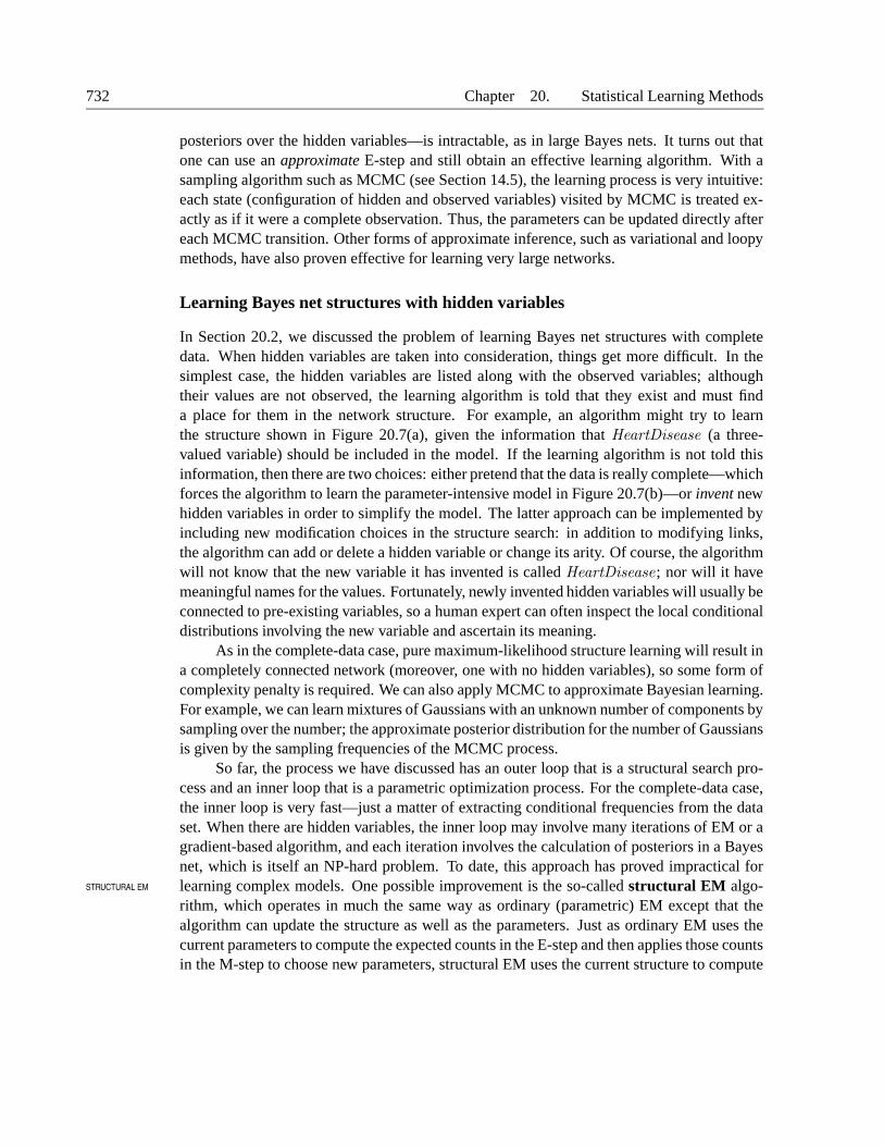
In Section 20.2, we discussed the problem of learning Bayes net structures with completedata. When hidden variables are taken into consideration, things get more difficult. In thesimplest case, the hidden variables are listed along with the observed variables; althoughtheir values are not observed, the learning algorithm is told that they exist and must finda place for them in the network structure. For example, an algorithm might try to learnthe structure shown in Figure 20.7(a), given the information that HeartDisease (a three-valued variable) should be included in the model. If the learning algorithm is not told thisinformation, then there are two choices: either pretend that the data is really complete—whichforces the algorithm to learn the parameter-intensive model in Figure 20.7(b)—or invent newhidden variables in order to simplify the model. The latter approach can be implemented byincluding new modification choices in the structure search: in addition to modifying links,the algorithm can add or delete a hidden variable or change its arity. Of course, the algorithmwill not know that the new variable it has invented is called HeartDisease; nor will it havemeaningful names for the values. Fortunately, newly invented hidden variables will usually beconnected to pre-existing variables, so a human expert can often inspect the local conditionaldistributions involving the new variable and ascertain its meaning.
As in the complete-data case, pure maximum-likelihood structure learning will result ina completely connected network (moreover, one with no hidden variables), so some form ofcomplexity penalty is required. We can also apply MCMC to approximate Bayesian learning.For example, we can learn mixtures of Gaussians with an unknown number of components bysampling over the number; the approximate posterior distribution for the number of Gaussiansis given by the sampling frequencies of the MCMC process.
So far, the process we have discussed has an outer loop that is a structural search pro-cess and an inner loop that is a parametric optimization process. For the complete-data case,the inner loop is very fast—just a matter of extracting conditional frequencies from the dataset. When there are hidden variables, the inner loop may involve many iterations of EM or agradient-based algorithm, and each iteration involves the calculation of posteriors in a Bayesnet, which is itself an NP-hard problem. To date, this approach has proved impractical forlearning complex models. One possible improvement is the so-called structural EM algo-STRUCTURAL EM
rithm, which operates in much the same way as ordinary (parametric) EM except that thealgorithm can update the structure as well as the parameters. Just as ordinary EM uses thecurrent parameters to compute the expected counts in the E-step and then applies those countsin the M-step to choose new parameters, structural EM uses the current structure to compute
Section 20.4. Instance-Based Learning 733
expected counts and then applies those counts in the M-step to evaluate the likelihood forpotential new structures. (This contrasts with the outer-loop/inner-loop method, which com-putes new expected counts for each potential structure.) In this way, structural EM may makeseveral structural alterations to the network without once recomputing the expected counts,and is capable of learning nontrivial Bayes net structures. Nonetheless, much work remainsto be done before we can say that the structure learning problem is solved.
20.4 INSTANCE-BASED LEARNING
So far, our discussion of statistical learning has focused primarily on fitting the parameters ofa restricted family of probability models to an unrestricted data set. For example, unsuper-vised clustering using mixtures of Gaussians assumes that the data are explained by the suma fixed number of Gaussian distributions. We call such methods parametric learning. Para-PARAMETRIC
LEARNING
metric learning methods are often simple and effective, but assuming a particular restrictedfamily of models often oversimplifies what’s happening in the real world, from where thedata come. Now, it is true when we have very little data, we cannot hope to learn a complexand detailed model, but it seems silly to keep the hypothesis complexity fixed even when thedata set grows very large!
In contrast to parametric learning, nonparametric learning methods allow the hypoth-NONPARAMETRICLEARNING
esis complexity to grow with the data. The more data we have, the wigglier the hypothesiscan be. We will look at two very simple families of nonparametric instance-based learningINSTANCE-BASED
LEARNING
(or memory-based learning) methods, so called because they construct hypotheses directlyfrom the training instances themselves.
Nearest-neighbor models
The key idea of nearest-neighbor models is that the properties of any particular input point xNEAREST-NEIGHBOR
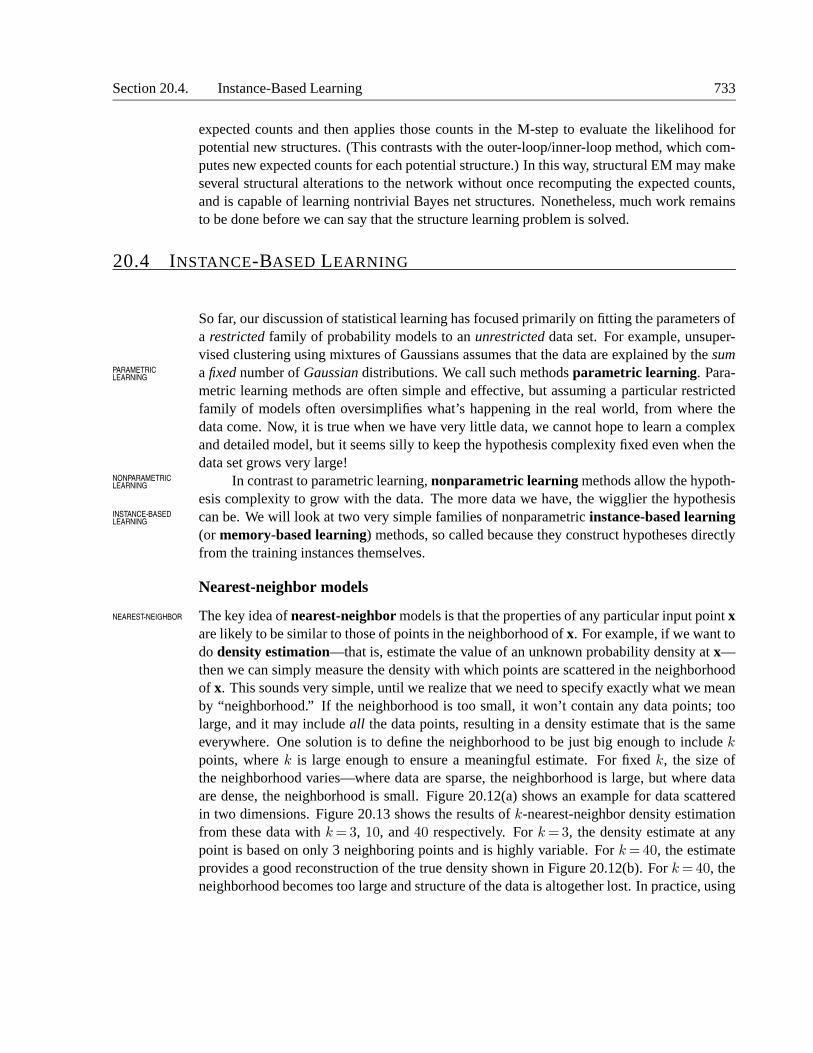
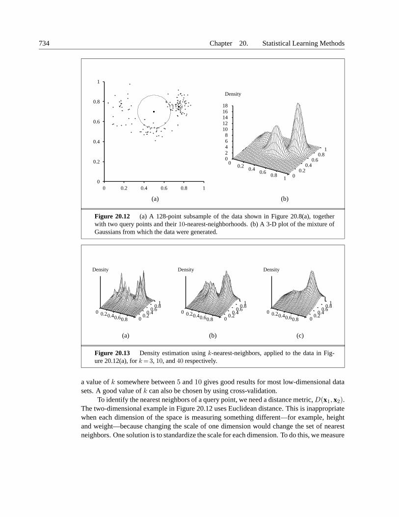
are likely to be similar to those of points in the neighborhood of x. For example, if we want todo density estimation—that is, estimate the value of an unknown probability density at x—then we can simply measure the density with which points are scattered in the neighborhoodof x. This sounds very simple, until we realize that we need to specify exactly what we meanby “neighborhood.” If the neighborhood is too small, it won’t contain any data points; toolarge, and it may include all the data points, resulting in a density estimate that is the sameeverywhere. One solution is to define the neighborhood to be just big enough to include kpoints, where k is large enough to ensure a meaningful estimate. For fixed k, the size ofthe neighborhood varies—where data are sparse, the neighborhood is large, but where dataare dense, the neighborhood is small. Figure 20.12(a) shows an example for data scatteredin two dimensions. Figure 20.13 shows the results of k-nearest-neighbor density estimationfrom these data with k = 3, 10, and 40 respectively. For k =3, the density estimate at anypoint is based on only 3 neighboring points and is highly variable. For k = 40, the estimateprovides a good reconstruction of the true density shown in Figure 20.12(b). For k = 40, theneighborhood becomes too large and structure of the data is altogether lost. In practice, using
734 Chapter 20. Statistical Learning Methods
0
0.2
0.4
0.6
0.8
1
0 0.2 0.4 0.6 0.8 1
00.2
0.40.6
0.81 0
0.20.4
0.60.8
1
02468
1012141618
Density
(a) (b)
Figure 20.12 (a) A 128-point subsample of the data shown in Figure 20.8(a), togetherwith two query points and their 10-nearest-neighborhoods. (b) A 3-D plot of the mixture ofGaussians from which the data were generated.
0 0.20.40.60.8 00.2
0.40.6
0.81
Density
0 0.20.40.60.8 00.2
0.40.6
0.81
Density
0 0.20.40.60.8 00.2
0.40.6
0.81
Density
(a) (b) (c)
Figure 20.13 Density estimation using k-nearest-neighbors, applied to the data in Fig-ure 20.12(a), for k = 3, 10, and 40 respectively.
a value of k somewhere between 5 and 10 gives good results for most low-dimensional datasets. A good value of k can also be chosen by using cross-validation.
To identify the nearest neighbors of a query point, we need a distance metric, D(x1, x2).The two-dimensional example in Figure 20.12 uses Euclidean distance. This is inappropriatewhen each dimension of the space is measuring something different—for example, heightand weight—because changing the scale of one dimension would change the set of nearestneighbors. One solution is to standardize the scale for each dimension. To do this, we measure
Section 20.4. Instance-Based Learning 735
the standard deviation of each feature over the whole data set and express feature values asmultiples of the standard deviation for that feature. (This is a special case of the Mahalanobisdistance, which takes into account the covariance of the features as well.) Finally, for discreteMAHALANOBIS
DISTANCE
features we can use the Hamming distance, which defines D(x1, x2) to be the number ofHAMMING DISTANCE
features on which x1 and x2 differ.Density estimates like those shown in Figure 20.13 define joint distributions over the
input space. Unlike a Bayesian network, however, an instance-based representation cannotcontain hidden variables, which means that we cannot perform unsupervised clustering as wedid with the mixture-of-Gaussians model. We can still use the density estimate to predict atarget value y given input feature values x by calculating P (y|x)= P (y, x)/P (x), providedthat the training data include values for the target feature.
It is also possible to use the nearest-neighbor idea for direct supervised learning. Givena test example with input x, the output y =h(x) is obtained from the y-values of the k nearestneighbors of x. In the discrete case, we can obtain a single prediction by majority vote. In thecontinuous case, we can average the k values or do local linear regression, fitting a hyperplaneto the k points and predicting the value at x according to the hyperplane.
The k-nearest-neighbor learning algorithm is very simple to implement, requires littlein the way of tuning, and often performs quite well. It is a good thing to try first on anew learning problem. For large data sets, however, we require an efficient mechanism forfinding the nearest neighbors of a query point x—simply calculating the distance to everypoint would take far too long. A variety of ingenious methods have been proposed to makethis step efficient by preprocessing the training data. Unfortunately, most of these methodsdo not scale well with the dimension of the space (i.e., the number of features).
High-dimensional spaces pose an additional problem, namely that nearest neighbors insuch spaces are usually a long way away! Consider a data set of size N in the d-dimensionalunit hypercube, and assume hypercubic neighborhoods of side b and volume bd. (The sameargument works with hyperspheres, but the formula for the volume of a hypersphere is morecomplicated.) To contain k points, the average neighborhood must occupy a fraction k/Nof the entire volume, which is 1. Hence, bd = k/N , or b= (k/N)1/d. So far, so good. Nowlet the number of features d be 100 and let k be 10 and N be 1,000,000. Then we have b ≈0.89—that is, the neighborhood has to span almost the entire input space! This suggests thatnearest-neighbor methods cannot be trusted for high-dimensional data. In low dimensionsthere is no problem; with d = 2 we have b = 0.003.
Kernel models
In a kernel model, we view each training instance as generating a little density function—aKERNEL MODEL
kernel function—of its own. The density estimate as a whole is just the normalized sum ofKERNEL FUNCTION
all the little kernel functions. A training instance at xi will generate a kernel function K(x, xi)that assigns a probability to each point x in the space. Thus, the density estimate is
P (x) =1
N
N∑
i=1
K(x, xi) .
736 Chapter 20. Statistical Learning Methods
0 0.20.40.60.8 00.2
0.40.6
0.81
Density
0 0.20.40.60.8 00.2
0.40.6
0.81
Density
0 0.20.40.60.8 00.2
0.40.6
0.81
Density
(a) (b) (c)
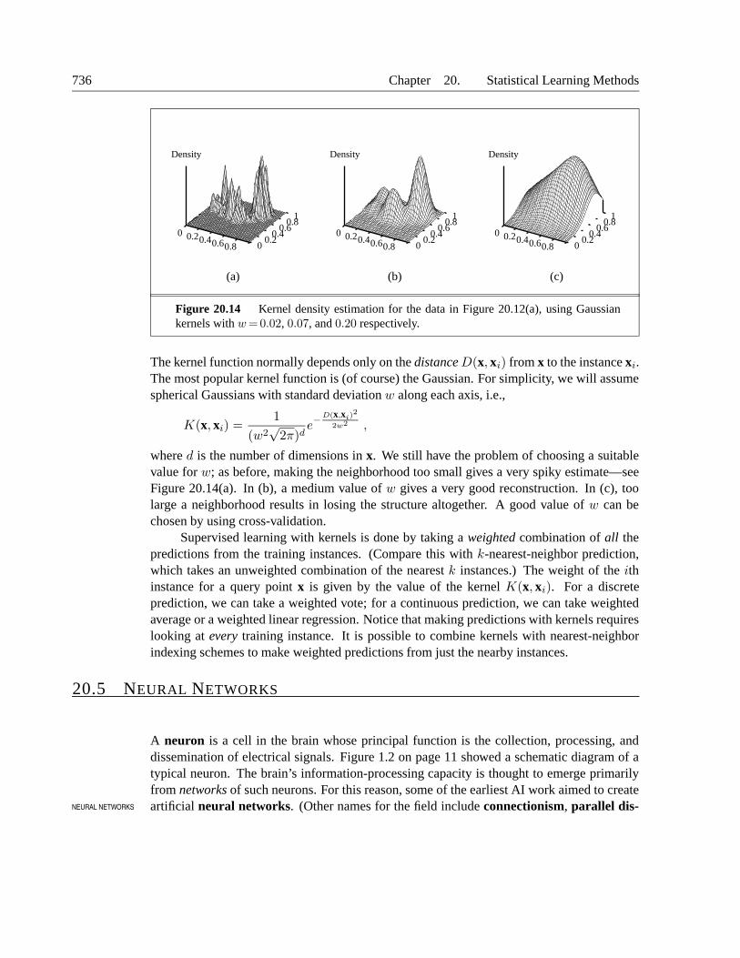
Figure 20.14 Kernel density estimation for the data in Figure 20.12(a), using Gaussiankernels with w =0.02, 0.07, and 0.20 respectively.
The kernel function normally depends only on the distance D(x, xi) from x to the instance xi.The most popular kernel function is (of course) the Gaussian. For simplicity, we will assumespherical Gaussians with standard deviation w along each axis, i.e.,
K(x, xi) =1
(w2√
2π)de−
D(x,xi)2
2w2 ,
where d is the number of dimensions in x. We still have the problem of choosing a suitablevalue for w; as before, making the neighborhood too small gives a very spiky estimate—seeFigure 20.14(a). In (b), a medium value of w gives a very good reconstruction. In (c), toolarge a neighborhood results in losing the structure altogether. A good value of w can bechosen by using cross-validation.
Supervised learning with kernels is done by taking a weighted combination of all thepredictions from the training instances. (Compare this with k-nearest-neighbor prediction,which takes an unweighted combination of the nearest k instances.) The weight of the ithinstance for a query point x is given by the value of the kernel K(x, xi). For a discreteprediction, we can take a weighted vote; for a continuous prediction, we can take weightedaverage or a weighted linear regression. Notice that making predictions with kernels requireslooking at every training instance. It is possible to combine kernels with nearest-neighborindexing schemes to make weighted predictions from just the nearby instances.
20.5 NEURAL NETWORKS
A neuron is a cell in the brain whose principal function is the collection, processing, anddissemination of electrical signals. Figure 1.2 on page 11 showed a schematic diagram of atypical neuron. The brain’s information-processing capacity is thought to emerge primarilyfrom networks of such neurons. For this reason, some of the earliest AI work aimed to createartificial neural networks. (Other names for the field include connectionism, parallel dis-NEURAL NETWORKS
Section 20.5. Neural Networks 737
tributed processing, and neural computation.) Figure 20.15 shows a simple mathematicalmodel of the neuron devised by McCulloch and Pitts (1943). Roughly speaking, it “fires”when a linear combination of its inputs exceeds some threshold. Since 1943, much moredetailed and realistic models have been developed, both for neurons and for larger systemsin the brain, leading to the modern field of computational neuroscience. On the other hand,COMPUTATIONAL
NEUROSCIENCE
researchers in AI and statistics became interested in the more abstract properties of neuralnetworks, such as their ability to perform distributed computation, to tolerate noisy inputs,and to learn. Although we understand now that other kinds of systems—including Bayesiannetworks—have these properties, neural networks remain one of the most popular and effec-tive forms of learning system and are worthy of study in their own right.
Units in neural networks
Neural networks are composed of nodes or units (see Figure 20.15) connected by directedUNITS
links. A link from unit j to unit i serves to propagate the activation aj from j to i. Each linkLINKS
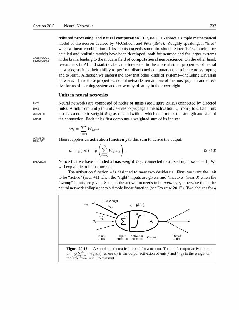
ACTIVATION also has a numeric weight Wj,i associated with it, which determines the strength and sign ofWEIGHT the connection. Each unit i first computes a weighted sum of its inputs:
ini =n∑
j =0
Wj,iaj .
Then it applies an activation function g to this sum to derive the output:ACTIVATIONFUNCTION
ai = g(ini) = g
n∑
j =0
Wj,iaj
. (20.10)
Notice that we have included a bias weight W0,i connected to a fixed input a0 = − 1. WeBIAS WEIGHT
will explain its role in a moment.The activation function g is designed to meet two desiderata. First, we want the unit
to be “active” (near +1) when the “right” inputs are given, and “inactive” (near 0) when the“wrong” inputs are given. Second, the activation needs to be nonlinear, otherwise the entireneural network collapses into a simple linear function (see Exercise 20.17). Two choices for g
Output
ΣInput Links
Activation Function
Input Function
Output Links
a0 = −1 ai = g(ini)
ai
giniWj,i
W0,i
Bias Weight
aj
Figure 20.15 A simple mathematical model for a neuron. The unit’s output activation isai = g(
∑n
j = 0Wj,iaj), where aj is the output activation of unit j and Wj,i is the weight on
the link from unit j to this unit.
738 Chapter 20. Statistical Learning Methods
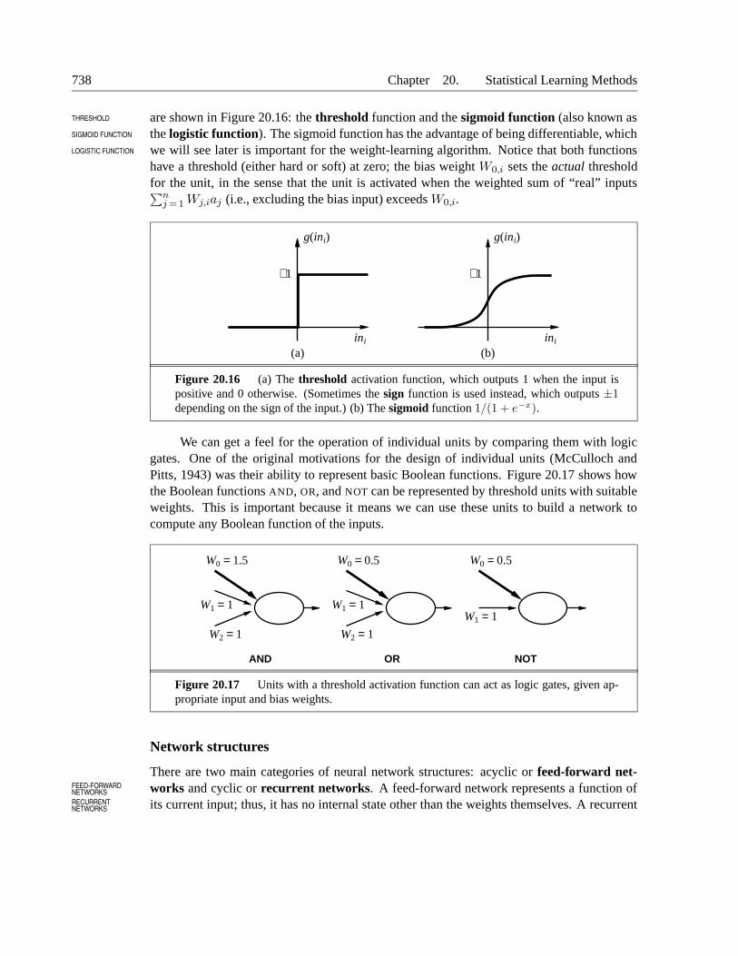
are shown in Figure 20.16: the threshold function and the sigmoid function (also known asTHRESHOLD
SIGMOID FUNCTION the logistic function). The sigmoid function has the advantage of being differentiable, whichLOGISTIC FUNCTION we will see later is important for the weight-learning algorithm. Notice that both functions
have a threshold (either hard or soft) at zero; the bias weight W0,i sets the actual thresholdfor the unit, in the sense that the unit is activated when the weighted sum of “real” inputs∑n
j =1 Wj,iaj (i.e., excluding the bias input) exceeds W0,i.
(a) (b)
+1 +1
iniini
g(ini)g(ini)
Figure 20.16 (a) The threshold activation function, which outputs 1 when the input ispositive and 0 otherwise. (Sometimes the sign function is used instead, which outputs ±1depending on the sign of the input.) (b) The sigmoid function 1/(1 + e−x).
We can get a feel for the operation of individual units by comparing them with logicgates. One of the original motivations for the design of individual units (McCulloch andPitts, 1943) was their ability to represent basic Boolean functions. Figure 20.17 shows howthe Boolean functions AND, OR, and NOT can be represented by threshold units with suitableweights. This is important because it means we can use these units to build a network tocompute any Boolean function of the inputs.
AND
W0 = 1.5
W1 = 1
W2 = 1
OR
W2 = 1
W1 = 1
W0 = 0.5
NOT
W1 = 1
W0 = 0.5
Figure 20.17 Units with a threshold activation function can act as logic gates, given ap-propriate input and bias weights.
Network structures
There are two main categories of neural network structures: acyclic or feed-forward net-works and cyclic or recurrent networks. A feed-forward network represents a function ofFEED-FORWARD
NETWORKSRECURRENTNETWORKS its current input; thus, it has no internal state other than the weights themselves. A recurrent
Section 20.5. Neural Networks 739
network, on the other hand, feeds its outputs back into its own inputs. This means that theactivation levels of the network form a dynamical system that may reach a stable state or ex-hibit oscillations or even chaotic behavior. Moreover, the response of the network to a giveninput depends on its initial state, which may depend on previous inputs. Hence, recurrentnetworks (unlike feed-forward networks) can support short-term memory. This makes themmore interesting as models of the brain, but also more difficult to understand. This sectionwill concentrate on feed-forward networks; some pointers for further reading on recurrentnetworks are given at the end of the chapter.
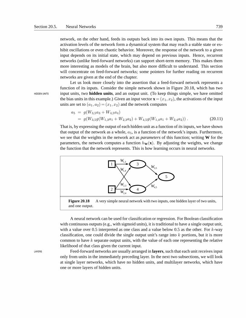
Let us look more closely into the assertion that a feed-forward network represents afunction of its inputs. Consider the simple network shown in Figure 20.18, which has twoinput units, two hidden units, and an output unit. (To keep things simple, we have omittedHIDDEN UNITS
the bias units in this example.) Given an input vector x = (x1, x2), the activations of the inputunits are set to (a1, a2)= (x1, x2) and the network computes
a5 = g(W3,5a3 + W4,5a4)
= g(W3,5g(W1,3a1 + W2,3a2) + W4,5g(W1,4a1 + W2,4a2)) . (20.11)
That is, by expressing the output of each hidden unit as a function of its inputs, we have shownthat output of the network as a whole, a5, is a function of the network’s inputs. Furthermore,we see that the weights in the network act as parameters of this function; writing W for theparameters, the network computes a function hW(x). By adjusting the weights, we changethe function that the network represents. This is how learning occurs in neural networks.
W 1, 3
1, 4 W
2, 3 W
2, 4 W
W 3, 5
4, 5 W
1
2
3
4
5
Figure 20.18 A very simple neural network with two inputs, one hidden layer of two units,and one output.
A neural network can be used for classification or regression. For Boolean classificationwith continuous outputs (e.g., with sigmoid units), it is traditional to have a single output unit,with a value over 0.5 interpreted as one class and a value below 0.5 as the other. For k-wayclassification, one could divide the single output unit’s range into k portions, but it is morecommon to have k separate output units, with the value of each one representing the relativelikelihood of that class given the current input.
Feed-forward networks are usually arranged in layers, such that each unit receives inputLAYERS
only from units in the immediately preceding layer. In the next two subsections, we will lookat single layer networks, which have no hidden units, and multilayer networks, which haveone or more layers of hidden units.
740 Chapter 20. Statistical Learning Methods
Output Units
Input Units Wj,i
-4 -2 0 2 4x1-4
-20
24
x2
00.10.20.30.40.50.60.70.80.9
1Perceptron output
(a) (b)
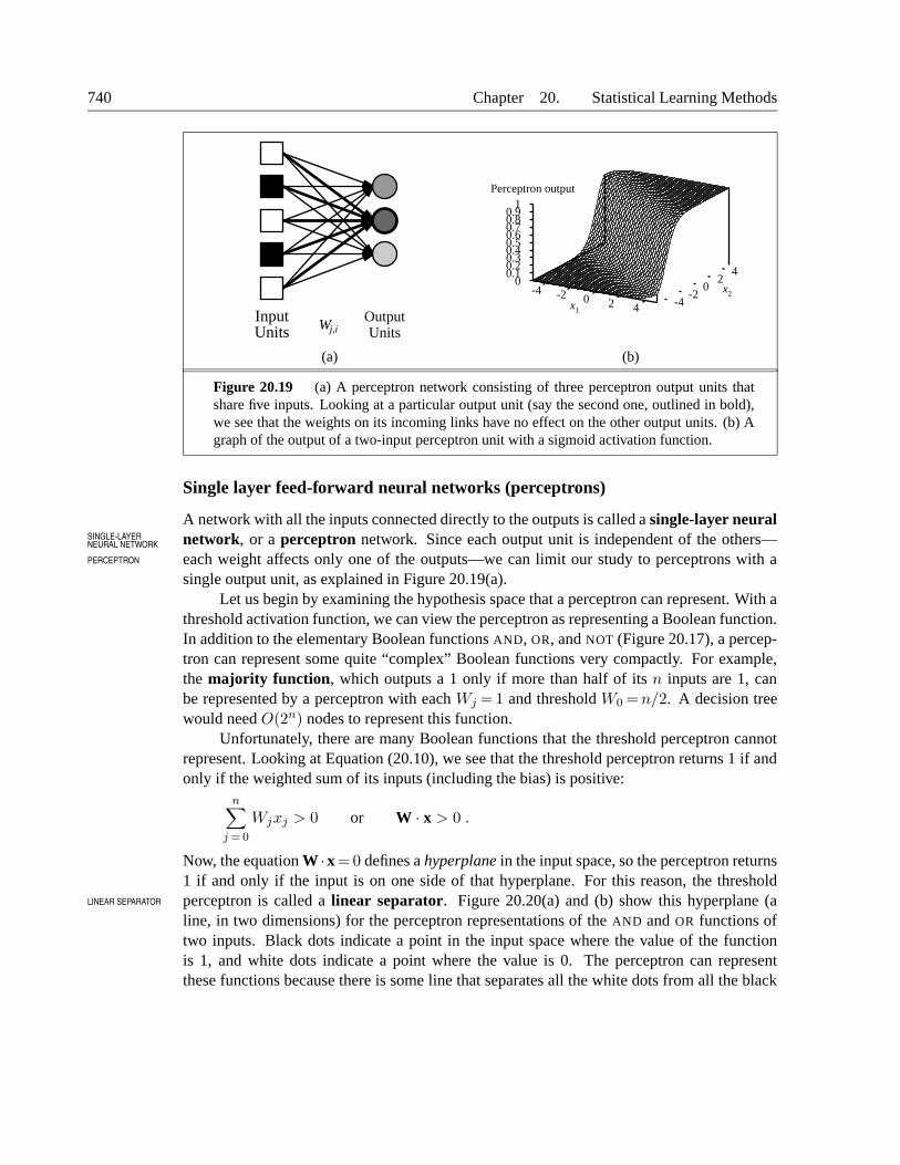
Figure 20.19 (a) A perceptron network consisting of three perceptron output units thatshare five inputs. Looking at a particular output unit (say the second one, outlined in bold),we see that the weights on its incoming links have no effect on the other output units. (b) Agraph of the output of a two-input perceptron unit with a sigmoid activation function.
Single layer feed-forward neural networks (perceptrons)
A network with all the inputs connected directly to the outputs is called a single-layer neuralnetwork, or a perceptron network. Since each output unit is independent of the others—SINGLE-LAYER
NEURAL NETWORK
PERCEPTRON each weight affects only one of the outputs—we can limit our study to perceptrons with asingle output unit, as explained in Figure 20.19(a).
Let us begin by examining the hypothesis space that a perceptron can represent. With athreshold activation function, we can view the perceptron as representing a Boolean function.In addition to the elementary Boolean functions AND, OR, and NOT (Figure 20.17), a percep-tron can represent some quite “complex” Boolean functions very compactly. For example,the majority function, which outputs a 1 only if more than half of its n inputs are 1, canbe represented by a perceptron with each Wj = 1 and threshold W0 = n/2. A decision treewould need O(2n) nodes to represent this function.
Unfortunately, there are many Boolean functions that the threshold perceptron cannotrepresent. Looking at Equation (20.10), we see that the threshold perceptron returns 1 if andonly if the weighted sum of its inputs (including the bias) is positive:
n∑
j =0
Wjxj > 0 or W · x > 0 .
Now, the equation W ·x = 0 defines a hyperplane in the input space, so the perceptron returns1 if and only if the input is on one side of that hyperplane. For this reason, the thresholdperceptron is called a linear separator. Figure 20.20(a) and (b) show this hyperplane (aLINEAR SEPARATOR
line, in two dimensions) for the perceptron representations of the AND and OR functions oftwo inputs. Black dots indicate a point in the input space where the value of the functionis 1, and white dots indicate a point where the value is 0. The perceptron can representthese functions because there is some line that separates all the white dots from all the black
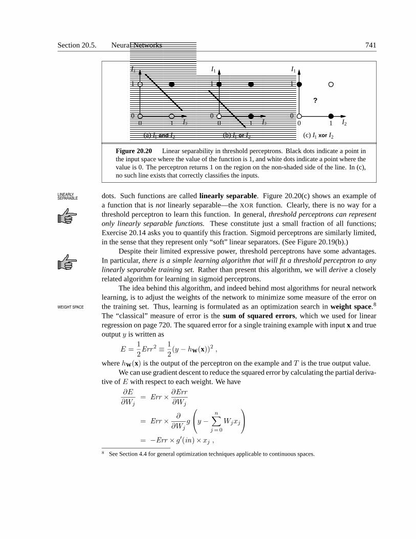
Section 20.5. Neural Networks 741
(a) I1 and I2
1
00 1
I1
I2
(b) I1 or I2
0 1
1
0
I1
I2
(c) I1 xor I2
?
0 1
1
0
I1
I2
Figure 20.20 Linear separability in threshold perceptrons. Black dots indicate a point inthe input space where the value of the function is 1, and white dots indicate a point where thevalue is 0. The perceptron returns 1 on the region on the non-shaded side of the line. In (c),no such line exists that correctly classifies the inputs.
dots. Such functions are called linearly separable. Figure 20.20(c) shows an example ofLINEARLYSEPARABLE
a function that is not linearly separable—the XOR function. Clearly, there is no way for athreshold perceptron to learn this function. In general, threshold perceptrons can representonly linearly separable functions. These constitute just a small fraction of all functions;Exercise 20.14 asks you to quantify this fraction. Sigmoid perceptrons are similarly limited,in the sense that they represent only “soft” linear separators. (See Figure 20.19(b).)
Despite their limited expressive power, threshold perceptrons have some advantages.In particular, there is a simple learning algorithm that will fit a threshold perceptron to anylinearly separable training set. Rather than present this algorithm, we will derive a closelyrelated algorithm for learning in sigmoid perceptrons.
The idea behind this algorithm, and indeed behind most algorithms for neural networklearning, is to adjust the weights of the network to minimize some measure of the error onthe training set. Thus, learning is formulated as an optimization search in weight space.8WEIGHT SPACE
The “classical” measure of error is the sum of squared errors, which we used for linearregression on page 720. The squared error for a single training example with input x and trueoutput y is written as
E =1
2Err2 ≡ 1
2(y − hW(x))2 ,
where hW(x) is the output of the perceptron on the example and T is the true output value.We can use gradient descent to reduce the squared error by calculating the partial deriva-
tive of E with respect to each weight. We have∂E
∂Wj= Err × ∂Err
∂Wj
= Err × ∂
∂Wjg
y −n∑
j =0
Wjxj
= −Err × g′(in)×xj ,
8 See Section 4.4 for general optimization techniques applicable to continuous spaces.
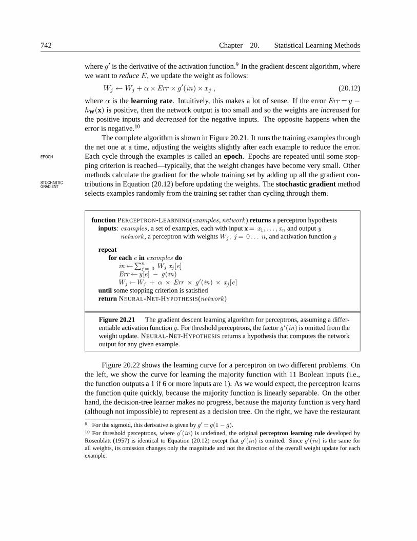
742 Chapter 20. Statistical Learning Methods
where g′ is the derivative of the activation function.9 In the gradient descent algorithm, wherewe want to reduce E, we update the weight as follows:
Wj ←Wj + α×Err × g′(in)×xj , (20.12)
where α is the learning rate. Intuitively, this makes a lot of sense. If the error Err = y −hW(x) is positive, then the network output is too small and so the weights are increased forthe positive inputs and decreased for the negative inputs. The opposite happens when theerror is negative.10
The complete algorithm is shown in Figure 20.21. It runs the training examples throughthe net one at a time, adjusting the weights slightly after each example to reduce the error.Each cycle through the examples is called an epoch. Epochs are repeated until some stop-EPOCH
ping criterion is reached—typically, that the weight changes have become very small. Othermethods calculate the gradient for the whole training set by adding up all the gradient con-tributions in Equation (20.12) before updating the weights. The stochastic gradient methodSTOCHASTIC
GRADIENT
selects examples randomly from the training set rather than cycling through them.
function PERCEPTRON-LEARNING(examples ,network ) returns a perceptron hypothesisinputs: examples , a set of examples, each with input x = x1, . . . , xn and output y
network , a perceptron with weights Wj , j = 0 . . . n, and activation function g
repeatfor each e in examples do
in←∑n
j = 0Wj xj [e]
Err← y [e] − g(in)Wj←Wj + α × Err × g ′(in) × xj [e]
until some stopping criterion is satisfiedreturn NEURAL-NET-HYPOTHESIS(network )
Figure 20.21 The gradient descent learning algorithm for perceptrons, assuming a differ-entiable activation function g. For threshold perceptrons, the factor g ′(in) is omitted from theweight update. NEURAL-NET-HYPOTHESIS returns a hypothesis that computes the networkoutput for any given example.
Figure 20.22 shows the learning curve for a perceptron on two different problems. Onthe left, we show the curve for learning the majority function with 11 Boolean inputs (i.e.,the function outputs a 1 if 6 or more inputs are 1). As we would expect, the perceptron learnsthe function quite quickly, because the majority function is linearly separable. On the otherhand, the decision-tree learner makes no progress, because the majority function is very hard(although not impossible) to represent as a decision tree. On the right, we have the restaurant
9 For the sigmoid, this derivative is given by g′ = g(1− g).10 For threshold perceptrons, where g′(in) is undefined, the original perceptron learning rule developed byRosenblatt (1957) is identical to Equation (20.12) except that g′(in) is omitted. Since g′(in) is the same forall weights, its omission changes only the magnitude and not the direction of the overall weight update for eachexample.
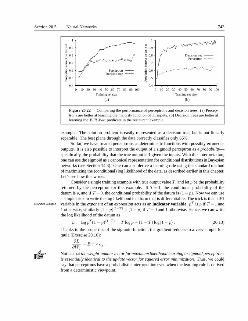
Section 20.5. Neural Networks 743
0.4
0.5
0.6
0.7
0.8
0.9
1
0 10 20 30 40 50 60 70 80 90 100
Prop
ortio
n co
rrec
t on
test
set
Training set size
PerceptronDecision tree
0.4
0.5
0.6
0.7
0.8
0.9
1
0 10 20 30 40 50 60 70 80 90 100
Prop
ortio
n co
rrec
t on
test
set
Training set size
Decision treePerceptron
(a) (b)
Figure 20.22 Comparing the performance of perceptrons and decision trees. (a) Percep-trons are better at learning the majority function of 11 inputs. (b) Decision trees are better atlearning the WillWait predicate in the restaurant example.
example. The solution problem is easily represented as a decision tree, but is not linearlyseparable. The best plane through the data correctly classifies only 65%.
So far, we have treated perceptrons as deterministic functions with possibly erroneousoutputs. It is also possible to interpret the output of a sigmoid perceptron as a probability—specifically, the probability that the true output is 1 given the inputs. With this interpretation,one can use the sigmoid as a canonical representation for conditional distributions in Bayesiannetworks (see Section 14.3). One can also derive a learning rule using the standard methodof maximizing the (conditional) log likelihood of the data, as described earlier in this chapter.Let’s see how this works.
Consider a single training example with true output value T , and let p be the probabilityreturned by the perceptron for this example. If T =1, the conditional probability of thedatum is p, and if T =0, the conditional probability of the datum is (1− p). Now we can usea simple trick to write the log likelihood in a form that is differentiable. The trick is that a 0/1variable in the exponent of an expression acts as an indicator variable: pT is p if T = 1 andINDICATOR VARIABLE
1 otherwise; similarly (1− p)(1−T ) is (1− p) if T = 0 and 1 otherwise. Hence, we can writethe log likelihood of the datum as
L = log pT (1− p)(1−T ) = T log p + (1− T ) log(1− p) . (20.13)
Thanks to the properties of the sigmoid function, the gradient reduces to a very simple for-mula (Exercise 20.16):
∂L
∂Wj= Err × aj .
Notice that the weight-update vector for maximum likelihood learning in sigmoid perceptronsis essentially identical to the update vector for squared error minimization. Thus, we couldsay that perceptrons have a probabilistic interpretation even when the learning rule is derivedfrom a deterministic viewpoint.
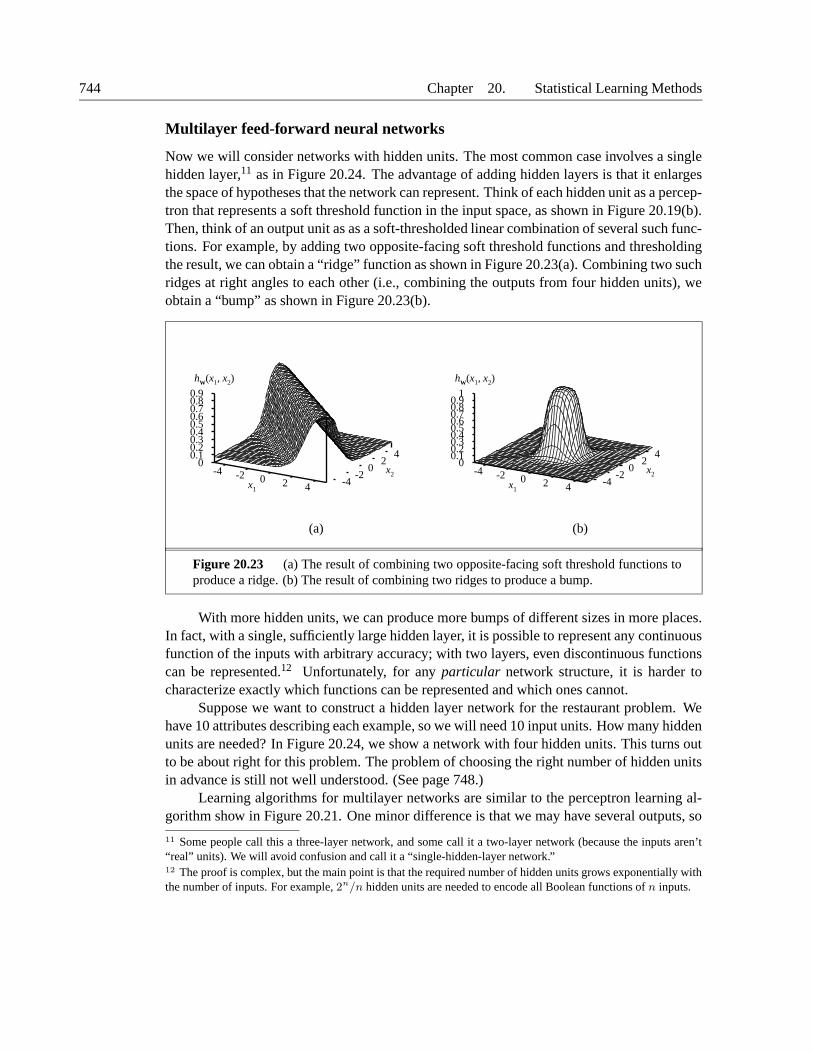
744 Chapter 20. Statistical Learning Methods
Multilayer feed-forward neural networks
Now we will consider networks with hidden units. The most common case involves a singlehidden layer,11 as in Figure 20.24. The advantage of adding hidden layers is that it enlargesthe space of hypotheses that the network can represent. Think of each hidden unit as a percep-tron that represents a soft threshold function in the input space, as shown in Figure 20.19(b).Then, think of an output unit as as a soft-thresholded linear combination of several such func-tions. For example, by adding two opposite-facing soft threshold functions and thresholdingthe result, we can obtain a “ridge” function as shown in Figure 20.23(a). Combining two suchridges at right angles to each other (i.e., combining the outputs from four hidden units), weobtain a “bump” as shown in Figure 20.23(b).
-4 -2 0 2 4x1-4
-20
24
x2
00.10.20.30.40.50.60.70.80.9
hW(x1, x2)
-4 -2 0 2 4x1-4
-20
24
x2
00.10.20.30.40.50.60.70.80.9
1
hW(x1, x2)
(a) (b)
Figure 20.23 (a) The result of combining two opposite-facing soft threshold functions toproduce a ridge. (b) The result of combining two ridges to produce a bump.
With more hidden units, we can produce more bumps of different sizes in more places.In fact, with a single, sufficiently large hidden layer, it is possible to represent any continuousfunction of the inputs with arbitrary accuracy; with two layers, even discontinuous functionscan be represented.12 Unfortunately, for any particular network structure, it is harder tocharacterize exactly which functions can be represented and which ones cannot.
Suppose we want to construct a hidden layer network for the restaurant problem. Wehave 10 attributes describing each example, so we will need 10 input units. How many hiddenunits are needed? In Figure 20.24, we show a network with four hidden units. This turns outto be about right for this problem. The problem of choosing the right number of hidden unitsin advance is still not well understood. (See page 748.)
Learning algorithms for multilayer networks are similar to the perceptron learning al-gorithm show in Figure 20.21. One minor difference is that we may have several outputs, so
11 Some people call this a three-layer network, and some call it a two-layer network (because the inputs aren’t“real” units). We will avoid confusion and call it a “single-hidden-layer network.”12 The proof is complex, but the main point is that the required number of hidden units grows exponentially withthe number of inputs. For example, 2n/n hidden units are needed to encode all Boolean functions of n inputs.
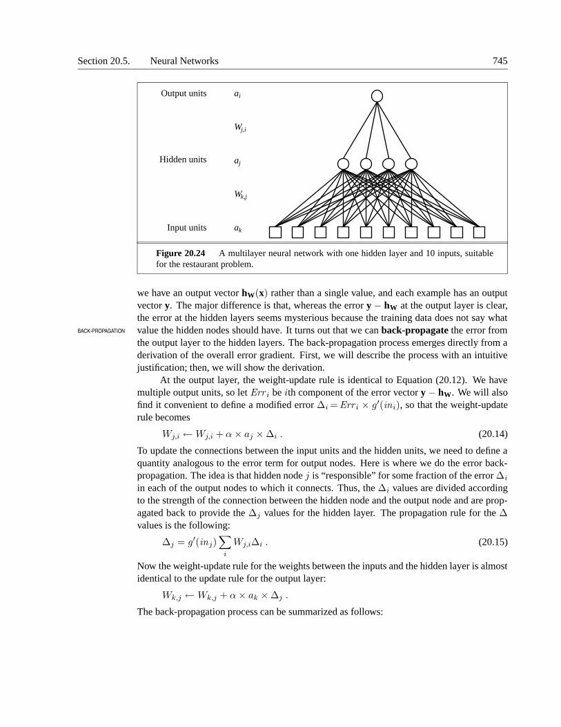
Section 20.5. Neural Networks 745
Input units
Hidden units
Output units ai
Wj,i
aj
Wk,j
ak
Figure 20.24 A multilayer neural network with one hidden layer and 10 inputs, suitablefor the restaurant problem.
we have an output vector hW(x) rather than a single value, and each example has an outputvector y. The major difference is that, whereas the error y − hW at the output layer is clear,the error at the hidden layers seems mysterious because the training data does not say whatvalue the hidden nodes should have. It turns out that we can back-propagate the error fromBACK-PROPAGATION
the output layer to the hidden layers. The back-propagation process emerges directly from aderivation of the overall error gradient. First, we will describe the process with an intuitivejustification; then, we will show the derivation.
At the output layer, the weight-update rule is identical to Equation (20.12). We havemultiple output units, so let Err i be ith component of the error vector y − hW. We will alsofind it convenient to define a modified error ∆i =Err i × g′(ini), so that the weight-updaterule becomes
Wj,i ←Wj,i + α× aj ×∆i . (20.14)
To update the connections between the input units and the hidden units, we need to define aquantity analogous to the error term for output nodes. Here is where we do the error back-propagation. The idea is that hidden node j is “responsible” for some fraction of the error ∆i
in each of the output nodes to which it connects. Thus, the ∆i values are divided accordingto the strength of the connection between the hidden node and the output node and are prop-agated back to provide the ∆j values for the hidden layer. The propagation rule for the ∆values is the following:
∆j = g′(inj)∑
i
Wj,i∆i . (20.15)
Now the weight-update rule for the weights between the inputs and the hidden layer is almostidentical to the update rule for the output layer:
Wk,j ←Wk,j + α× ak ×∆j .
The back-propagation process can be summarized as follows:
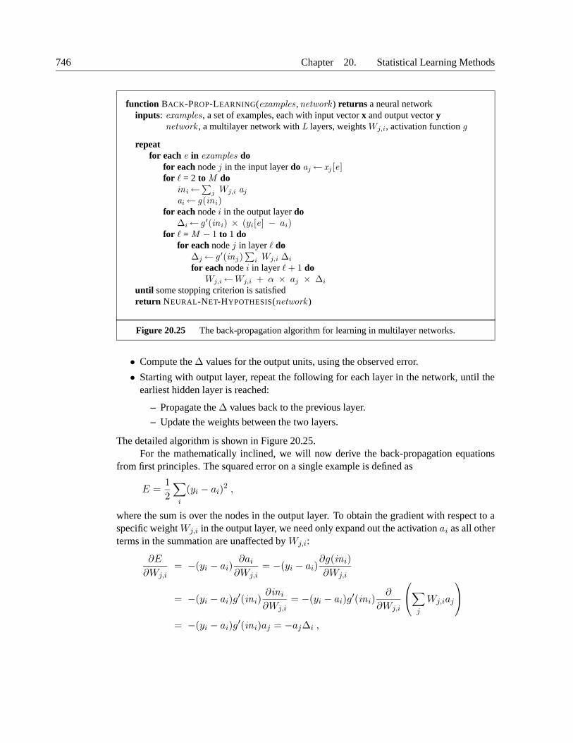
746 Chapter 20. Statistical Learning Methods
function BACK-PROP-LEARNING(examples ,network ) returns a neural networkinputs: examples , a set of examples, each with input vector x and output vector y
network , a multilayer network with L layers, weights Wj,i, activation function g
repeatfor each e in examples do
for each node j in the input layer do aj← xj [e]for ` = 2 to M do
ini←∑
j Wj,i aj
ai← g(ini)for each node i in the output layer do
∆i← g ′(ini) × (yi[e] − ai)for ` = M − 1 to 1 do
for each node j in layer ` do∆j← g ′(inj)
∑
i Wj,i ∆i
for each node i in layer ` + 1 doWj,i←Wj,i + α × aj × ∆i
until some stopping criterion is satisfiedreturn NEURAL-NET-HYPOTHESIS(network )
Figure 20.25 The back-propagation algorithm for learning in multilayer networks.
• Compute the ∆ values for the output units, using the observed error.
• Starting with output layer, repeat the following for each layer in the network, until theearliest hidden layer is reached:
– Propagate the ∆ values back to the previous layer.
– Update the weights between the two layers.
The detailed algorithm is shown in Figure 20.25.For the mathematically inclined, we will now derive the back-propagation equations
from first principles. The squared error on a single example is defined as
E =1
2
∑
i
(yi − ai)2 ,
where the sum is over the nodes in the output layer. To obtain the gradient with respect to aspecific weight Wj,i in the output layer, we need only expand out the activation ai as all otherterms in the summation are unaffected by Wj,i:
∂E
∂Wj,i= −(yi − ai)
∂ai
∂Wj,i= −(yi − ai)
∂g(ini)
∂Wj,i
= −(yi − ai)g′(ini)
∂ini
∂Wj,i= −(yi − ai)g
′(ini)∂
∂Wj,i
∑
j
Wj,iaj
= −(yi − ai)g′(ini)aj = −aj∆i ,

Section 20.5. Neural Networks 747
with ∆i defined as before. To obtain the gradient with respect to the Wk,j weights connectingthe input layer to the hidden layer, we have to keep the entire summation over i becauseeach output value ai may be affected by changes in Wk,j . We also have to expand out theactivations aj . We will show the derivation in gory detail because it is interesting to see howthe derivative operator propagates back through the network:
∂E
∂Wk,j= −
∑
i
(yi − ai)∂ai
∂Wk,j= −
∑
i
(yi − ai)∂g(ini)
∂Wk,j
= −∑
i
(yi − ai)g′(ini)
∂ini
∂Wk,j= −
∑
i
∆i∂
∂Wk,j
∑
j
Wj,iaj
= −∑
i
∆iWj,i∂aj
∂Wk,j= −
∑
i
∆iWj,i∂g(inj)
∂Wk,j
= −∑
i
∆iWj,ig′(inj)
∂inj
∂Wk,j
= −∑
i
∆iWj,ig′(inj)
∂
∂Wk,j
(
∑
k
Wk,jak
)
= −∑
i
∆iWj,ig′(inj)ak = −ak∆j ,
where ∆j is defined as before. Thus, we obtain the update rules obtained earlier from intuitiveconsiderations. It is also clear that the process can be continued for networks with more thanone hidden layer, which justifies the general algorithm given in Figure 20.25.
Having made it through (or skipped over) all the mathematics, let’s see how a single-hidden-layer network performs on the restaurant problem. In Figure 20.26, we show two
0
2
4
6
8
10
12
14
0 50 100 150 200 250 300 350 400
Tot
al e
rror
on
trai
ning
set
Number of epochs
0.4
0.5
0.6
0.7
0.8
0.9
1
0 10 20 30 40 50 60 70 80 90 100
Prop
ortio
n co
rrec
t on
test
set
Training set size
Decision treeMultilayer network
(a) (b)
Figure 20.26 (a) Training curve showing the gradual reduction in error as weights aremodified over several epochs, for a given set of examples in the restaurant domain. (b)Comparative learning curves showing that decision-tree learning does slightly better thanback-propagation in a multilayer network.
748 Chapter 20. Statistical Learning Methods
curves. The first is a training curve, which shows the mean squared error on a given trainingTRAINING CURVE
set of 100 restaurant examples during the weight-updating process. This demonstrates thatthe network does indeed converge to a perfect fit to the training data. The second curve is thestandard learning curve for the restaurant data. The neural network does learn well, althoughnot quite as fast as decision-tree learning; this is perhaps not surprising, because the data weregenerated from a simple decision tree in the first place.
Neural networks are capable of far more complex learning tasks of course, although itmust be said that a certain amount of twiddling is needed to get the network structure rightand to achieve convergence to something close to the global optimum in weight space. Thereare literally tens of thousands of published applications of neural networks. Section 20.7looks at one such application in more depth.
Learning neural network structures
So far, we have considered the problem of learning weights, given a fixed network structure;just as with Bayesian networks, we also need to understand how to find the best networkstructure. If we choose a network that is too big, it will be able to memorize all the examplesby forming a large lookup table, but will not necessarily generalize well to inputs that havenot been seen before.13 In other words, like all statistical models, neural networks are subjectto overfitting when there are too many parameters in the model. We saw this in Figure 18.1(page 652), where the high-parameter models in (b) and (c) fit all the data, but might notgeneralize as well as the low-parameter models in (a) and (d).
If we stick to fully connected networks, the only choices to be made concern the numberof hidden layers and their sizes. The usual approach is to try several and keep the best. Thecross-validation techniques of Chapter 18 are needed if we are to avoid peeking at the testset. That is, we choose the network architecture that gives the highest prediction accuracy onthe validation sets.
If we want to consider networks that are not fully connected, then we need to findsome effective search method through the very large space of possible connection topologies.The optimal brain damage algorithm begins with a fully connected network and removesOPTIMAL BRAIN
DAMAGE
connections from it. After the network is trained for the first time, an information-theoreticapproach identifies an optimal selection of connections that can be dropped. The networkis then retrained, and if its performance has not decreased then the process is repeated. Inaddition to removing connections, it is also possible to remove units that are not contributingmuch to the result.
Several algorithms have been proposed for growing a larger network from a smaller one.One, the tiling algorithm, resembles decision-list learning. The idea is to start with a singleTILING
unit that does its best to produce the correct output on as many of the training examples aspossible. Subsequent units are added to take care of the examples that the first unit got wrong.The algorithm adds only as many units as are needed to cover all the examples.
13 It has been observed that very large networks do generalize well as long as the weights are kept small. Thisrestriction keeps the activation values in the linear region of the sigmoid function g(x) where x is close to zero.This, in turn, means that the network behaves like a linear function (Exercise 20.17) with far fewer parameters.
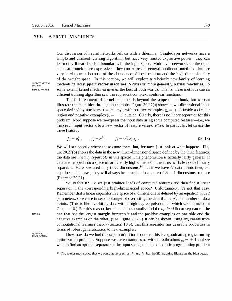
Section 20.6. Kernel Machines 749
20.6 KERNEL MACHINES
Our discussion of neural networks left us with a dilemma. Single-layer networks have asimple and efficient learning algorithm, but have very limited expressive power—they canlearn only linear decision boundaries in the input space. Multilayer networks, on the otherhand, are much more expressive—they can represent general nonlinear functions—but arevery hard to train because of the abundance of local minima and the high dimensionalityof the weight space. In this section, we will explore a relatively new family of learningmethods called support vector machines (SVMs) or, more generally, kernel machines. ToSUPPORT VECTOR
MACHINE
KERNEL MACHINE some extent, kernel machines give us the best of both worlds. That is, these methods use anefficient training algorithm and can represent complex, nonlinear functions.
The full treatment of kernel machines is beyond the scope of the book, but we canillustrate the main idea through an example. Figure 20.27(a) shows a two-dimensional inputspace defined by attributes x = (x1, x2), with positive examples (y = + 1) inside a circularregion and negative examples (y = − 1) outside. Clearly, there is no linear separator for thisproblem. Now, suppose we re-express the input data using some computed features—i.e., wemap each input vector x to a new vector of feature values, F (x). In particular, let us use thethree features
f1 =x21 , f2 = x2
2 , f3 =√
2x1x2 . (20.16)
We will see shortly where these came from, but, for now, just look at what happens. Fig-ure 20.27(b) shows the data in the new, three-dimensional space defined by the three features;the data are linearly separable in this space! This phenomenon is actually fairly general: ifdata are mapped into a space of sufficiently high dimension, then they will always be linearlyseparable. Here, we used only three dimensions,14 but if we have N data points then, ex-cept in special cases, they will always be separable in a space of N − 1 dimensions or more(Exercise 20.21).
So, is that it? Do we just produce loads of computed features and then find a linearseparator in the corresponding high-dimensional space? Unfortunately, it’s not that easy.Remember that a linear separator in a space of d dimensions is defined by an equation with dparameters, so we are in serious danger of overfitting the data if d ≈ N , the number of datapoints. (This is like overfitting data with a high-degree polynomial, which we discussed inChapter 18.) For this reason, kernel machines usually find the optimal linear separator—theone that has the largest margin between it and the positive examples on one side and theMARGIN
negative examples on the other. (See Figure 20.28.) It can be shown, using arguments fromcomputational learning theory (Section 18.5), that this separator has desirable properties interms of robust generalization to new examples.
Now, how do we find this separator? It turns out that this is a quadratic programmingQUADRATICPROGRAMMING
optimization problem. Suppose we have examples xi with classifications yi = ± 1 and wewant to find an optimal separator in the input space; then the quadratic programming problem
14 The reader may notice that we could have used just f1 and f2, but the 3D mapping illustrates the idea better.
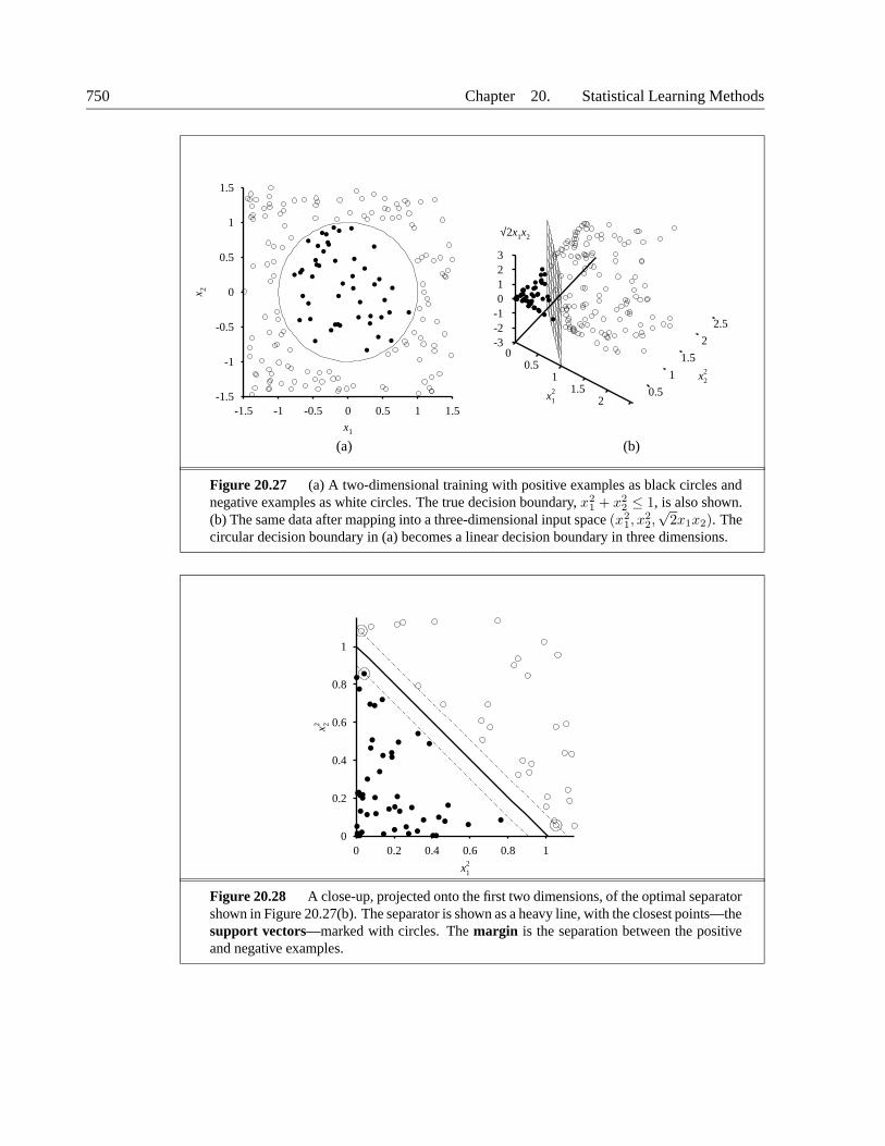
750 Chapter 20. Statistical Learning Methods
-1.5
-1
-0.5
0
0.5
1
1.5
-1.5 -1 -0.5 0 0.5 1 1.5
x 2
x1
00.5
11.5
2x12 0.5
1
1.5
2
2.5
x22
-3-2-10123
√2x1x2
(a) (b)
Figure 20.27 (a) A two-dimensional training with positive examples as black circles andnegative examples as white circles. The true decision boundary, x2
1 + x22 ≤ 1, is also shown.
(b) The same data after mapping into a three-dimensional input space (x21, x
22,√
2x1x2). Thecircular decision boundary in (a) becomes a linear decision boundary in three dimensions.
0
0.2
0.4
0.6
0.8
1
0 0.2 0.4 0.6 0.8 1
x 22
x12
Figure 20.28 A close-up, projected onto the first two dimensions, of the optimal separatorshown in Figure 20.27(b). The separator is shown as a heavy line, with the closest points—thesupport vectors—marked with circles. The margin is the separation between the positiveand negative examples.
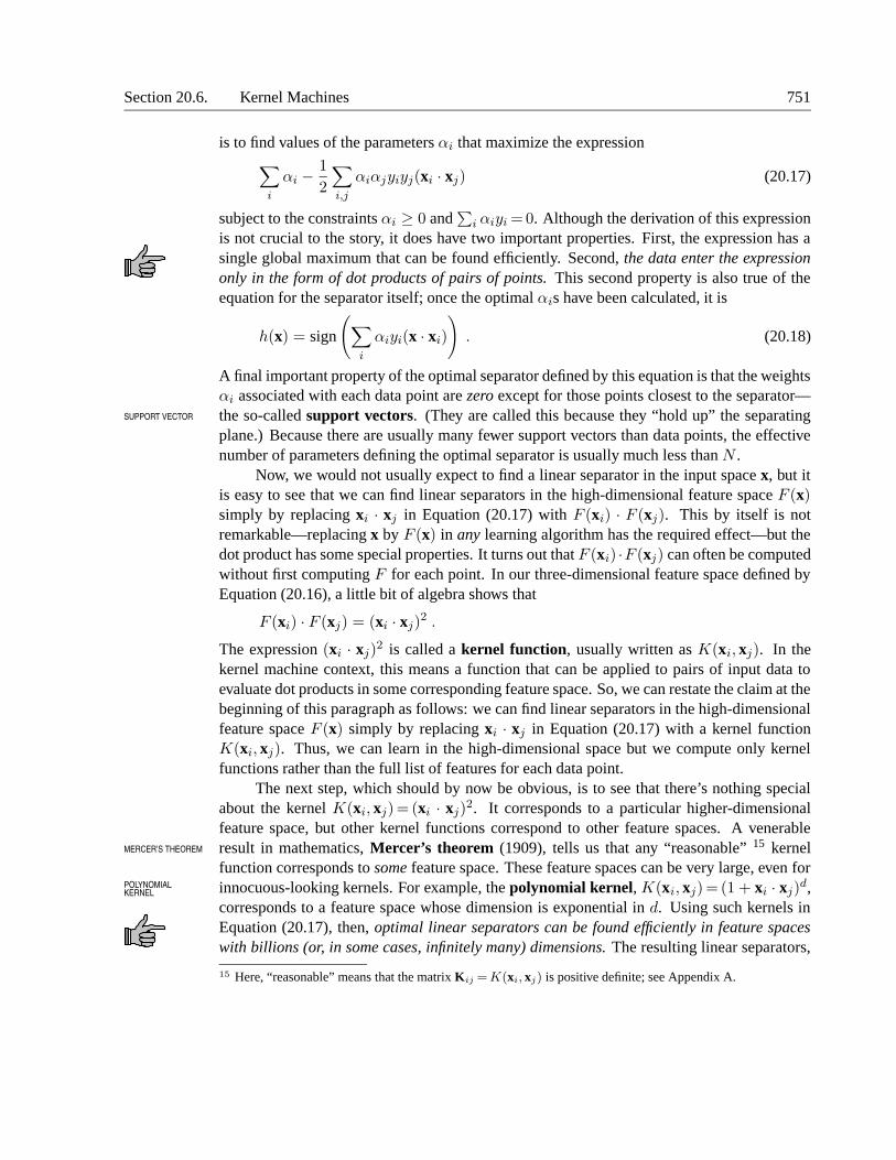
Section 20.6. Kernel Machines 751
is to find values of the parameters αi that maximize the expression∑
i
αi −1
2
∑
i,j
αiαjyiyj(xi · xj) (20.17)
subject to the constraints αi ≥ 0 and∑
i αiyi = 0. Although the derivation of this expressionis not crucial to the story, it does have two important properties. First, the expression has asingle global maximum that can be found efficiently. Second, the data enter the expressiononly in the form of dot products of pairs of points. This second property is also true of theequation for the separator itself; once the optimal αis have been calculated, it is
h(x) = sign
(
∑
i
αiyi(x · xi)
)
. (20.18)
A final important property of the optimal separator defined by this equation is that the weightsαi associated with each data point are zero except for those points closest to the separator—the so-called support vectors. (They are called this because they “hold up” the separatingSUPPORT VECTOR
plane.) Because there are usually many fewer support vectors than data points, the effectivenumber of parameters defining the optimal separator is usually much less than N .
Now, we would not usually expect to find a linear separator in the input space x, but itis easy to see that we can find linear separators in the high-dimensional feature space F (x)simply by replacing xi · xj in Equation (20.17) with F (xi) · F (xj). This by itself is notremarkable—replacing x by F (x) in any learning algorithm has the required effect—but thedot product has some special properties. It turns out that F (xi) ·F (xj) can often be computedwithout first computing F for each point. In our three-dimensional feature space defined byEquation (20.16), a little bit of algebra shows that
F (xi) · F (xj) = (xi · xj)2 .
The expression (xi · xj)2 is called a kernel function, usually written as K(xi, xj). In the
kernel machine context, this means a function that can be applied to pairs of input data toevaluate dot products in some corresponding feature space. So, we can restate the claim at thebeginning of this paragraph as follows: we can find linear separators in the high-dimensionalfeature space F (x) simply by replacing xi · xj in Equation (20.17) with a kernel functionK(xi, xj). Thus, we can learn in the high-dimensional space but we compute only kernelfunctions rather than the full list of features for each data point.
The next step, which should by now be obvious, is to see that there’s nothing specialabout the kernel K(xi, xj)= (xi · xj)
2. It corresponds to a particular higher-dimensionalfeature space, but other kernel functions correspond to other feature spaces. A venerableresult in mathematics, Mercer’s theorem (1909), tells us that any “reasonable” 15 kernelMERCER’S THEOREM
function corresponds to some feature space. These feature spaces can be very large, even forinnocuous-looking kernels. For example, the polynomial kernel, K(xi, xj)= (1 + xi · xj)
d,POLYNOMIALKERNEL
corresponds to a feature space whose dimension is exponential in d. Using such kernels inEquation (20.17), then, optimal linear separators can be found efficiently in feature spaceswith billions (or, in some cases, infinitely many) dimensions. The resulting linear separators,
15 Here, “reasonable” means that the matrix Kij = K(xi, xj) is positive definite; see Appendix A.
752 Chapter 20. Statistical Learning Methods
when mapped back to the original input space, can correspond to arbitrarily wiggly, nonlinearboundaries between the positive and negative examples.
We mentioned in the preceding section that kernel machines excel at handwritten digitrecognition; they are rapidly being adopted for other applications—especially those withmany input features. As part of this process, many new kernels have been designed thatwork with strings, trees, and other non-numerical data types. It has also been observed thatthe kernel method can be applied not only with learning algorithms that find optimal linearseparators, but also with any other algorithm that can be reformulated to work only with dotproducts of pairs of data points, as in Equations 20.17 and 20.18. Once this is done, the dotproduct is replaced by a kernel function and we have a kernelized version of the algorithm.KERNELIZATION
This can be done easily for k-nearest-neighbor and perceptron learning, among others.
20.7 CASE STUDY: HANDWRITTEN DIGIT RECOGNITION
Recognizing handwritten digits is an important problem with many applications, includingautomated sorting of mail by postal code, automated reading of checks and tax returns, anddata entry for hand-held computers. It is an area where rapid progress has been made, in partbecause of better learning algorithms and in part because of the availability of better trainingsets. The United States National Institute of Science and Technology (NIST) has archived adatabase of 60,000 labeled digits, each 20× 20= 400 pixels with 8-bit grayscale values. Ithas become one of the standard benchmark problems for comparing new learning algorithms.Some example digits are shown in Figure 20.29.
Figure 20.29 Examples from the NIST database of handwritten digits. Top row: examplesof digits 0–9 that are easy to identify. Bottom row: more difficult examples of the same digits.
Many different learning approaches have been tried. One of the first, and probably thesimplest, is the 3-nearest-neighbor classifier, which also has the advantage of requiring notraining time. As a memory-based algorithm, however, it must store all 60,000 images, andits runtime performance is slow. It achieved a test error rate of 2.4%.
A single-hidden-layer neural network was designed for this problem with 400 inputunits (one per pixel) and 10 output units (one per class). Using cross-validation, it was foundthat roughly 300 hidden units gave the best performance. With full interconnections betweenlayers, there were a total of 123,300 weights. This network achieved a 1.6% error rate.
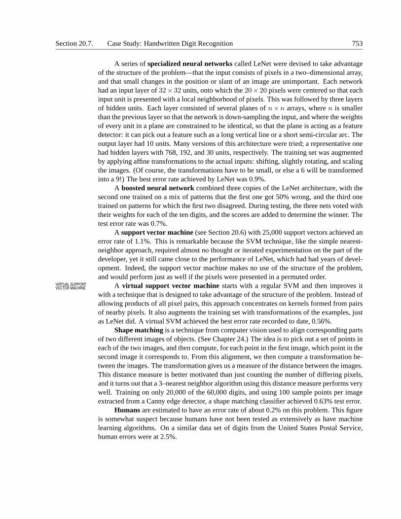
Section 20.7. Case Study: Handwritten Digit Recognition 753
A series of specialized neural networks called LeNet were devised to take advantageof the structure of the problem—that the input consists of pixels in a two–dimensional array,and that small changes in the position or slant of an image are unimportant. Each networkhad an input layer of 32× 32 units, onto which the 20× 20 pixels were centered so that eachinput unit is presented with a local neighborhood of pixels. This was followed by three layersof hidden units. Each layer consisted of several planes of n×n arrays, where n is smallerthan the previous layer so that the network is down-sampling the input, and where the weightsof every unit in a plane are constrained to be identical, so that the plane is acting as a featuredetector: it can pick out a feature such as a long vertical line or a short semi-circular arc. Theoutput layer had 10 units. Many versions of this architecture were tried; a representative onehad hidden layers with 768, 192, and 30 units, respectively. The training set was augmentedby applying affine transformations to the actual inputs: shifting, slightly rotating, and scalingthe images. (Of course, the transformations have to be small, or else a 6 will be transformedinto a 9!) The best error rate achieved by LeNet was 0.9%.
A boosted neural network combined three copies of the LeNet architecture, with thesecond one trained on a mix of patterns that the first one got 50% wrong, and the third onetrained on patterns for which the first two disagreed. During testing, the three nets voted withtheir weights for each of the ten digits, and the scores are added to determine the winner. Thetest error rate was 0.7%.
A support vector machine (see Section 20.6) with 25,000 support vectors achieved anerror rate of 1.1%. This is remarkable because the SVM technique, like the simple nearest-neighbor approach, required almost no thought or iterated experimentation on the part of thedeveloper, yet it still came close to the performance of LeNet, which had had years of devel-opment. Indeed, the support vector machine makes no use of the structure of the problem,and would perform just as well if the pixels were presented in a permuted order.
A virtual support vector machine starts with a regular SVM and then improves itVIRTUAL SUPPORTVECTOR MACHINE
with a technique that is designed to take advantage of the structure of the problem. Instead ofallowing products of all pixel pairs, this approach concentrates on kernels formed from pairsof nearby pixels. It also augments the training set with transformations of the examples, justas LeNet did. A virtual SVM achieved the best error rate recorded to date, 0.56%.
Shape matching is a technique from computer vision used to align corresponding partsof two different images of objects. (See Chapter 24.) The idea is to pick out a set of points ineach of the two images, and then compute, for each point in the first image, which point in thesecond image it corresponds to. From this alignment, we then compute a transformation be-tween the images. The transformation gives us a measure of the distance between the images.This distance measure is better motivated than just counting the number of differing pixels,and it turns out that a 3–nearest neighbor algorithm using this distance measure performs verywell. Training on only 20,000 of the 60,000 digits, and using 100 sample points per imageextracted from a Canny edge detector, a shape matching classifier achieved 0.63% test error.
Humans are estimated to have an error rate of about 0.2% on this problem. This figureis somewhat suspect because humans have not been tested as extensively as have machinelearning algorithms. On a similar data set of digits from the United States Postal Service,human errors were at 2.5%.
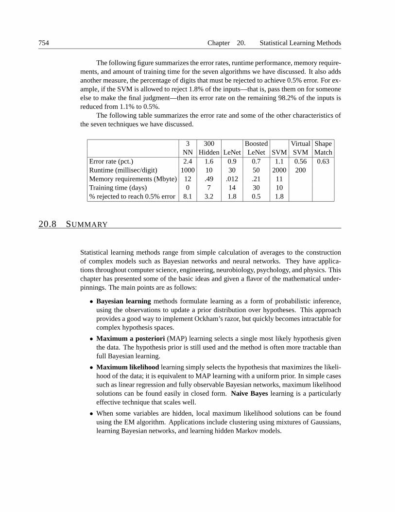
754 Chapter 20. Statistical Learning Methods
The following figure summarizes the error rates, runtime performance, memory require-ments, and amount of training time for the seven algorithms we have discussed. It also addsanother measure, the percentage of digits that must be rejected to achieve 0.5% error. For ex-ample, if the SVM is allowed to reject 1.8% of the inputs—that is, pass them on for someoneelse to make the final judgment—then its error rate on the remaining 98.2% of the inputs isreduced from 1.1% to 0.5%.
The following table summarizes the error rate and some of the other characteristics ofthe seven techniques we have discussed.
3 300 Boosted Virtual ShapeNN Hidden LeNet LeNet SVM SVM Match
Error rate (pct.) 2.4 1.6 0.9 0.7 1.1 0.56 0.63Runtime (millisec/digit) 1000 10 30 50 2000 200Memory requirements (Mbyte) 12 .49 .012 .21 11Training time (days) 0 7 14 30 10% rejected to reach 0.5% error 8.1 3.2 1.8 0.5 1.8
20.8 SUMMARY
Statistical learning methods range from simple calculation of averages to the constructionof complex models such as Bayesian networks and neural networks. They have applica-tions throughout computer science, engineering, neurobiology, psychology, and physics. Thischapter has presented some of the basic ideas and given a flavor of the mathematical under-pinnings. The main points are as follows:
• Bayesian learning methods formulate learning as a form of probabilistic inference,using the observations to update a prior distribution over hypotheses. This approachprovides a good way to implement Ockham’s razor, but quickly becomes intractable forcomplex hypothesis spaces.
• Maximum a posteriori (MAP) learning selects a single most likely hypothesis giventhe data. The hypothesis prior is still used and the method is often more tractable thanfull Bayesian learning.
• Maximum likelihood learning simply selects the hypothesis that maximizes the likeli-hood of the data; it is equivalent to MAP learning with a uniform prior. In simple casessuch as linear regression and fully observable Bayesian networks, maximum likelihoodsolutions can be found easily in closed form. Naive Bayes learning is a particularlyeffective technique that scales well.
• When some variables are hidden, local maximum likelihood solutions can be foundusing the EM algorithm. Applications include clustering using mixtures of Gaussians,learning Bayesian networks, and learning hidden Markov models.
Section 20.8. Summary 755
• Learning the structure of Bayesian networks is an example of model selection. Thisusually involves a discrete search in the space of structures. Some method is requiredfor trading off model complexity against degree of fit.
• Instance-based models represent a distribution using the collection of training in-stances. Thus, the number of parameters grows with the training set. Nearest-neighbormethods look at the instances nearest to the point in question, whereas kernel methodsform a distance-weighted combination of all the instances.
• Neural networks are complex nonlinear functions with many parameters. Their pa-rameters can be learned from noisy data and they have been used for thousands ofapplications.
• A perceptron is a feed-forward neural network with no hidden units that can representonly linearly separable functions. If the data are linearly separable, a simple weight-update rule can be used to fit the data exactly.
• Multilayer feed-forward neural networks can represent any function, given enoughunits. The back-propagation algorithm implements a gradient descent in parameterspace to minimize the output error.
Statistical learning continues to be a very active area of research. Enormous strides have beenmade in both theory and practice, to the point where it is possible to learn almost any modelfor which exact or approximate inference is feasible.
BIBLIOGRAPHICAL AND HISTORICAL NOTES
The application of statistical learning techniques in AI was an active area of research inthe early years (see Duda and Hart, 1973) but became separated from mainstream AI as thelatter field concentrated on symbolic methods. It continued in various forms—some explicitlyprobabilistic, others not—in areas such as pattern recognition (Devroye et al., 1996) andinformation retrieval (Salton and McGill, 1983). A resurgence of interest occurred shortlyafter the introduction of Bayesian network models in the late 1980s; at roughly the same time,a statistical view of neural network learning began to emerge. In the late 1990s, there wasa noticeable convergence of interests in machine learning, statistics, and neural networks,centered on methods for creating large probabilistic models from data.
The naive Bayes model is one of the oldest and simplest forms of Bayesian network,dating back to the 1950s. Its origins were mentioned in the notes at the end of Chapter 13. ispartially explained by Domingos and Pazzani (1997). A boosted form of naive Bayes learn-ing won the first KDD Cup data mining competition (Elkan, 1997). Heckerman (1998) givesan excellent introduction to the general problem of Bayes net learning. Bayesian parame-ter learning with Dirichlet priors for Bayesian networks was discussed by Spiegelhalter et al.(1993). The BUGS software package (Gilks et al., 1994) incorporates many of these ideas andprovides a very powerful tool for formulating and learning complex probability models. Thefirst algorithms for learning Bayes net structures used conditional independence tests (Pearl,1988; Pearl and Verma, 1991). Spirtes et al. (1993) developed a comprehensive approach
756 Chapter 20. Statistical Learning Methods
and the TETRAD package for Bayes net learning using similar ideas. Algorithmic improve-ments since then led to a clear victory in the 2001 KDD Cup data mining competition for aBayes net learning method (Cheng et al., 2002). (The specific task here was a bioinformaticsproblem with 139,351 features!) A structure-learning approach based on maximizing like-lihood was developed by Cooper and Herskovits (1992) and improved by Heckerman et al.(1994). Friedman and Goldszmidt (1996) pointed out the influence of the representation oflocal conditional distributions on the learned structure.
The general problem of learning probability models with hidden variables and missingdata was addressed by the EM algorithm (Dempster et al., 1977), which was abstracted fromseveral existing methods including the Baum–Welch algorithm for HMM learning (Baumand Petrie, 1966). (Dempster himself views EM as a schema rather than an algorithm, since agood deal of mathematical work may be required before it can be applied to a new family ofdistributions.) EM is now one of the most widely used algorithms in science, and McLachlanand Krishnan (1997) devote an entire book to the algorithm and its properties. The specificproblem of learning mixture models, including mixtures of Gaussians, is covered by Tittering-ton et al. (1985). Within AI, the first successful system that used EM for mixture modellingwas AUTOCLASS (Cheeseman et al., 1988; Cheeseman and Stutz, 1996). AUTOCLASS hasbeen applied to a number of real-world scientific classification tasks, including the discoveryof new types of stars from spectral data (Goebel et al., 1989) and new classes of proteins andintrons in DNA/protein sequence databases (Hunter and States, 1992).
An EM algorithm for learning Bayes nets with hidden variables was developed by Lau-ritzen (1995). Gradient-based techniques have also proved effective for Bayes nets as well asdynamic Bayes nets (Russell et al., 1995; Binder et al., 1997a). The structural EM algorithmwas developed by (Friedman, 1998). The ability to learn the structure of Bayesian networks isclosely connected to the issue of recovering causal information from data. That is, is it possi-ble to learn Bayes nets in such a way that the recovered network structure indicates real causalinfluences? For many years, statisticians avoided this question, believing that observationaldata (as opposed to data generated from experimental trials) could yield only correlationalinformation—after all, any two variables that appear related might in fact be influenced bythird, unknown causal factor rather than influencing each other directly. Pearl (2000) has pre-sented convincing arguments to the contrary, showing that there are in fact many cases wherecausality can be ascertained and developing the causal network formalism to express causesCAUSAL NETWORK
and the effects of intervention as well as ordinary conditional probabilities.Nearest-neighbor models date back at least to (Fix and Hodges, 1951) and have been a
standard tool in statistics and pattern recognition ever since. Within AI, they were popularizedby (Stanfill and Waltz, 1986), who investigated methods for adapting the distance metric tothe data. Hastie and Tibshirani (1996) developed a way to localize the metric to each pointin the space, depending on the distribution of data around that point. Efficient indexingschemes for finding nearest neighbors are studied within the algorithms community (see,e.g., Indyk, 2000). Kernel density estimation, also called Parzen window density estimation,was investigated initially by Rosenblatt (1956) and Parzen (1962). Since that time, a hugeliterature has developed investigating the properties of various estimators. Devroye (1987)gives a thorough introduction.
Section 20.8. Summary 757
The literature on neural networks is rather too large (approximately 100,000 papers todate) to cover in detail. Cowan and Sharp (1988b, 1988a) survey the early history, beginningwith the work of McCulloch and Pitts (1943). Norbert Wiener, a pioneer of cybernetics andcontrol theory (Wiener, 1948), worked with McCulloch and Pitts and influenced a number ofyoung researchers including Marvin Minsky, who may have been the first to develop a work-ing neural network in hardware in 1951 (see Minsky and Papert, 1988, pp. ix–x). Meanwhile,in Britain, W. Ross Ashby (also a pioneer of cybernetics; see Ashby, 1940), Alan Turing,Grey Walter, and others formed the Ratio Club for “those who had Wiener’s ideas beforeWiener’s book appeared.” Ashby’s Design for a Brain (1948, 1952) put forth the idea thatintelligence could be created by the use of homeostatic devices containing appropriate feed-back loops to achieve stable adaptive behavior. Turing (1948) wrote a research report titledIntelligent Machinery that begins with the sentence “I propose to investigate the question asto whether it is possible for machinery to show intelligent behaviour” and goes on to describea recurrent neural network architecture he called “B-type unorganized machines” and an ap-proach to training them. Unfortunately, the report went unpublished until 1969, and was allbut ignored until recently.
Frank Rosenblatt (1957) invented the modern “perceptron” and proved the percep-tron convergence theorem (1960), although it had been foreshadowed by purely mathemat-ical work outside the context of neural networks (Agmon, 1954; Motzkin and Schoenberg,1954). Some early work was also done on multilayer networks, including Gamba percep-trons (Gamba et al., 1961) and madalines (Widrow, 1962). Learning Machines (Nilsson,1965) covers much of this early work and more. The subsequent demise of early perceptronresearch efforts was hastened (or, the authors later claimed, merely explained) by the bookPerceptrons (Minsky and Papert, 1969), which lamented the field’s lack of mathematicalrigor. The book pointed out that single-layer perceptrons could represent only linearly sepa-rable concepts and noted the lack of effective learning algorithms for multilayer networks.
The papers in (Hinton and Anderson, 1981), based on a conference in San Diego in1979, can be regarded as marking the renaissance of connectionism. The two-volume “PDP”(Parallel Distributed Processing) anthology (Rumelhart et al., 1986a) and a short article inNature (Rumelhart et al., 1986b) attracted a great deal of attention—indeed, the number ofpapers on “neural networks” multiplied by a factor of 200 between 1980–84 and 1990–94.The analysis of neural networks using the physical theory of magnetic spin glasses (Amitet al., 1985) tightened the links between statistical mechanics and neural network theory—providing not only useful mathematical insights but also respectability. The back-propagationtechnique had been invented quite early (Bryson and Ho, 1969) but it was rediscovered severaltimes (Werbos, 1974; Parker, 1985).
Support vector machines were originated in the 1990s (Cortes and Vapnik, 1995) andare now the subject of a fast-growing literature, including textbooks such as Cristianini andShawe-Taylor (2000). They have proven to be very popular and effective for tasks such astext categorization (Joachims, 2001), bioinformatics research (Brown et al., 2000), and natu-ral language processing, such as the handwritten digit recognition of DeCoste and Scholkopf(2002). A related technique that also uses the “kernel trick” to implicitly represent an expo-nential feature space is the voted perceptron (Collins and Duffy, 2002).
758 Chapter 20. Statistical Learning Methods
The probabilistic interpretation of neural networks has several sources, including Baumand Wilczek (1988) and Bridle (1990). The role of the sigmoid function is discussed byJordan (1995). Bayesian parameter learning for neural networks was proposed by MacKay(1992) and is explored further by Neal (1996). The capacity of neural networks to representfunctions was investigated by Cybenko (1988, 1989), who showed that two hidden layers areenough to represent any function and a single layer is enough to represent any continuousfunction. The “optimal brain damage” method for removing useless connections is by LeCunet al. (1989), and Sietsma and Dow (1988) show how to remove useless units. The tilingalgorithm for growing larger structures is due to Mezard and Nadal (1989). LeCun et al.(1995) survey a number of algorithms for handwritten digit recognition. Improved error ratessince then were reported by Belongie et al. (2002) for shape matching and DeCoste andScholkopf (2002) for virtual support vectors.
The complexity of neural network learning has been investigated by researchers in com-putational learning theory. Early computational results were obtained by Judd (1990), whoshowed that the general problem of finding a set of weights consistent with a set of examplesis NP-complete, even under very restrictive assumptions. Some of the first sample complexityresults were obtained by Baum and Haussler (1989), who showed that the number of exam-ples required for effective learning grows as roughly W log W , where W is the number ofweights.16 Since then, a much more sophisticated theory has been developed (Anthony andBartlett, 1999), including the important result that the representational capacity of a networkdepends on the size of the weights as well as on their number.
The most popular kind of neural network that we did not cover is the radial basisfunction, or RBF, network. A radial basis function combines a weighted collection of kernelsRADIAL BASIS
FUNCTION
(usually Gaussians, of course) to do function approximation. RBF networks can be trained intwo phases: first, an unsupervised clustering approach is used to train the parameters of theGaussians—the means and variances—are trained, as in Section 20.3. In the second phase,the relative weights of the Gaussians are determined. This is a system of linear equations,which we know how to solve directly. Thus, both phases of RBF training have a nice benefit:the first phase is unsupervised, and thus does not require labelled training data, and the secondphase, although supervised, is efficient. See Bishop (1995) for more details.
Recurrent networks, in which units are linked in cycles, were mentioned in the chap-ter but not explored in depth. Hopfield networks (Hopfield, 1982) are probably the best-HOPFIELD
NETWORKS
understood class of recurrent networks. They use bidirectional connections with symmetricweights (i.e., Wi,j = Wj,i), all of the units are both input and output units, the activationfunction g is the sign function, and the activation levels can only be ±1. A Hopfield networkfunctions as an associative memory: after the network trains on a set of examples, a newASSOCIATIVE
MEMORY
stimulus will cause it to settle into an activation pattern corresponding to the example in thetraining set that most closely resembles the new stimulus. For example, if the training set con-sists of a set of photographs, and the new stimulus is a small piece of one of the photographs,then the network activation levels will reproduce the photograph from which the piece was
16 This approximately confirmed “Uncle Bernie’s rule.” The rule was named after Bernie Widrow, who recom-mended using roughly ten times as many examples as weights.
Section 20.8. Summary 759
taken. Notice that the original photographs are not stored separately in the network; eachweight is a partial encoding of all the photographs. One of the most interesting theoreticalresults is that Hopfield networks can reliably store up to 0.138N training examples, where Nis the number of units in the network.
Boltzmann machines (Hinton and Sejnowski, 1983, 1986) also use symmetric weights,BOLTZMANNMACHINES
but include hidden units. In addition, they use a stochastic activation function, such thatthe probability of the output being 1 is some function of the total weighted input. Boltz-mann machines therefore undergo state transitions that resemble a simulated annealing search(see Chapter 4) for the configuration that best approximates the training set. It turns out thatBoltzmann machines are very closely related to a special case of Bayesian networks evaluatedwith a stochastic simulation algorithm. (See Section 14.5.)
The first application of the ideas underlying kernel machines was by Aizerman et al.(1964), but the full development of the theory, under the heading of support vector machines,is due to Vladimir Vapnik and colleagues (Boser et al., 1992; Vapnik, 1998). Cristianiniand Shawe-Taylor (2000) and Scholkopf and Smola (2002) provide rigorous introductions; afriendlier exposition appears in the AI Magazine article by Cristianini and Scholkopf (2002).
The material in this chapter brings together work from the fields of statistics, patternrecognition, and neural networks, so the story has been told many times in many ways. Goodtexts on Bayesian statistics include those by DeGroot (1970), Berger (1985), and Gelmanet al. (1995). Hastie et al. (2001) provide an excellent introduction to statistical learningmethods. For pattern classification, the classic text for many years has been Duda and Hart(1973), now updated (Duda et al., 2001). For neural nets, Bishop (1995) and Ripley (1996)are the leading texts. The field of computational neuroscience is covered by Dayan and Ab-bott (2001). The most important conference on neural networks and related topics is theannual NIPS (Neural Information Processing Conference) conference, whose proceedingsare published as the series Advances in Neural Information Processing Systems. Papers onlearning Bayesian networks also appear in the Uncertainty in AI and Machine Learning con-ferences and in several statistics conferences. Journals specific to neural networks includeNeural Computation, Neural Networks, and the IEEE Transactions on Neural Networks.
EXERCISES
20.1 The data used for Figure 20.1 can be viewed as being generated by h5. For each of theother four hypotheses, generate a data set of length 100 and plot the corresponding graphs forP (hi|d1, . . . , dm) and P (Dm+1 = lime|d1, . . . , dm). Comment on your results.
20.2 Repeat Exercise 20.1, this time plotting the values of P (Dm+1 = lime|hMAP) andP (Dm+1 = lime|hML).
20.3 Suppose that Ann’s utilities for cherry and lime candies are cA and `A, whereas Bob’sutilities are cB and `B . (But once Ann has unwrapped a piece of candy, Bob won’t buy it.)Presumably, if Bob likes lime candies much more than Ann, it would be wise to sell for Ann
760 Chapter 20. Statistical Learning Methods
to sell her bag of candies once she is sufficiently sure of its lime content. On the other hand,if Ann unwraps too many candies in the process, the bag will be worth less. Discuss theproblem of determining the optimal point at which to sell the bag. Determine the expectedutility of the optimal procedure, given the prior distribution from Section 20.1.
20.4 Two statisticians go to the doctor and are both given the same prognosis: A 40%chance that the problem is the deadly disease A, and a 60% chance of the fatal disease B.Fortunately, there are anti-A and anti-B drugs that are inexpensive, 100% effective, and freeof side-effects. The statisticians have the choice of taking one drug, both, or neither. Whatwill the first statistician (an avid Bayesian) do? How about the second statistician, who alwaysuses the maximum likelihood hypothesis?
The doctor does some research and discovers that disease B actually comes in twoversions, dextro-B and levo-B, which are equally likely and equally treatable by the anti-Bdrug. Now that there are three hypotheses, what will the two statisticians do?
20.5 Explain how to apply the boosting method of Chapter 18 to naive Bayes learning. Testthe performance of the resulting algorithm on the restaurant learning problem.
20.6 Consider m data points (xj , yj), where the yjs are generated from the xjs according tothe linear Gaussian model in Equation (20.5). Find the values of θ1, θ2, and σ that maximizethe conditional log likelihood of the data.
20.7 Consider the noisy-OR model for fever described in Section 14.3. Explain how toapply maximum-likelihood learning to fit the parameters of such a model to a set of completedata. (Hint: use the chain rule for partial derivatives.)
20.8 This exercise investigates properties of the Beta distribution defined in Equation (20.6).
a. By integrating over the range [0, 1], show that the normalization constant for the dis-tribution beta[a, b] is given by α = Γ(a + b)/Γ(a)Γ(b) where Γ(x) is the Gammafunction, defined by Γ(x + 1)= x · Γ(x) and Γ(1)=1. (For integer x, Γ(x + 1)=x!.)GAMMA FUNCTION
b. Show that the mean is a/(a + b).
c. Find the mode(s) (the most likely value(s) of θ).
d. Describe the distribution beta[ε, ε] for very small ε. What happens as such a distributionis updated?
20.9 Consider an arbitrary Bayesian network, a complete data set for that network, and thelikelihood for the data set according to the network. Give a simple proof that the likelihoodof the data cannot decrease if we add a new link to the network and recompute the maximum-likelihood parameter values.
20.10 Consider the application of EM to learn the parameters for the network in Fig-ure 20.10(a), given the true parameters in Equation (20.7).
a. Explain why the EM algorithm would not work if there were just two attributes in themodel rather than three.
b. Show the calculations for the first iteration of EM starting from Equation (20.8).
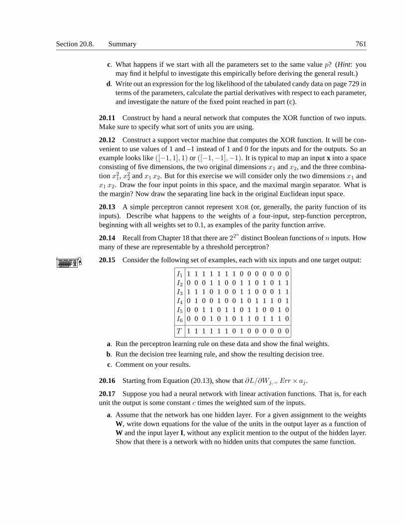
Section 20.8. Summary 761
c. What happens if we start with all the parameters set to the same value p? (Hint: youmay find it helpful to investigate this empirically before deriving the general result.)
d. Write out an expression for the log likelihood of the tabulated candy data on page 729 interms of the parameters, calculate the partial derivatives with respect to each parameter,and investigate the nature of the fixed point reached in part (c).
20.11 Construct by hand a neural network that computes the XOR function of two inputs.Make sure to specify what sort of units you are using.
20.12 Construct a support vector machine that computes the XOR function. It will be con-venient to use values of 1 and –1 instead of 1 and 0 for the inputs and for the outputs. So anexample looks like ([−1, 1], 1) or ([−1,−1],−1). It is typical to map an input x into a spaceconsisting of five dimensions, the two original dimensions x1 and x2, and the three combina-tion x2
1, x22 and x1 x2. But for this exercise we will consider only the two dimensions x1 and
x1 x2. Draw the four input points in this space, and the maximal margin separator. What isthe margin? Now draw the separating line back in the original Euclidean input space.
20.13 A simple perceptron cannot represent XOR (or, generally, the parity function of itsinputs). Describe what happens to the weights of a four-input, step-function perceptron,beginning with all weights set to 0.1, as examples of the parity function arrive.
20.14 Recall from Chapter 18 that there are 22ndistinct Boolean functions of n inputs. How
many of these are representable by a threshold perceptron?
20.15 Consider the following set of examples, each with six inputs and one target output:
I1 1 1 1 1 1 1 1 0 0 0 0 0 0 0I2 0 0 0 1 1 0 0 1 1 0 1 0 1 1I3 1 1 1 0 1 0 0 1 1 0 0 0 1 1I4 0 1 0 0 1 0 0 1 0 1 1 1 0 1I5 0 0 1 1 0 1 1 0 1 1 0 0 1 0I6 0 0 0 1 0 1 0 1 1 0 1 1 1 0
T 1 1 1 1 1 1 0 1 0 0 0 0 0 0
a. Run the perceptron learning rule on these data and show the final weights.
b. Run the decision tree learning rule, and show the resulting decision tree.
c. Comment on your results.
20.16 Starting from Equation (20.13), show that ∂L/∂Wj,= Err × aj .
20.17 Suppose you had a neural network with linear activation functions. That is, for eachunit the output is some constant c times the weighted sum of the inputs.
a. Assume that the network has one hidden layer. For a given assignment to the weightsW, write down equations for the value of the units in the output layer as a function ofW and the input layer I, without any explicit mention to the output of the hidden layer.Show that there is a network with no hidden units that computes the same function.

762 Chapter 20. Statistical Learning Methods
b. Repeat the calculation in part (a), this time for a network with any number of hiddenlayers. What can you conclude about linear activation functions?
20.18 Implement a data structure for layered, feed-forward neural networks, rememberingto provide the information needed for both forward evaluation and backward propagation.Using this data structure, write a function NEURAL-NETWORK-OUTPUT that takes an exam-ple and a network and computes the appropriate output values.
20.19 Suppose that a training set contains only a single example, repeated 100 times. In80 of the 100 cases, the single output value is 1; in the other 20, it is 0. What will a back-propagation network predict for this example, assuming that it has been trained and reachesa global optimum? (Hint: to find the global optimum, differentiate the error function and setto zero.)
20.20 The network in Figure 20.24 has four hidden nodes. This number was chosen some-what arbitrarily. Run systematic experiments to measure the learning curves for networkswith different numbers of hidden nodes. What is the optimal number? Would it be possibleto use a cross-validation method to find the best network before the fact?
20.21 Consider the problem of separating N data points into positive and negative examplesusing a linear separator. Clearly, this can always be done for N = 2 points on a line ofdimension d=1, regardless of how the points are labelled or where they are located (unlessthe points are in the same place).
a. Show that it can always be done for N = 3 points on a plane of dimension d= 2, unlessthey are collinear.
b. Show that it cannot always be done for N = 4 points on a plane of dimension d= 2.
c. Show that it can always be done for N =4 points in a space of dimension d= 3, unlessthey are coplanar.
d. Show that it cannot always be done for N = 5 points in a space of dimension d= 3.
e. The ambitious student may wish to prove that N points in general position (but notN + 1 are linearly separable in a space of dimension N − 1. From this it follows thatthe VC dimension (see Chapter 18) of linear halfspaces in dimension N − 1 is N .