2. linear programming
DESCRIPTION
ScienceTRANSCRIPT

[Page 29]
Chapter 2. Linear Programming: Model Formulation and Graphical Solution
[Page 30]
Many major decisions faced by a manager of a business focus on the best way to achieve the objectives of the firm, subject to the restrictions placed on the manager by the operating environment. These restrictions can take the form of limited resources, such as time, labor, energy, material, or money; or they can be in the form of restrictive guidelines, such as a recipe for making cereal or engineering specifications. One of the most frequent objectives of business firms is to gain the most profit possible or, in other words, to maximize profit. The objective of individual organizational units within a firm (such as a production or packaging department) is often to minimize cost. When a manager attempts to solve a general type of problem by seeking an objective that is subject to restrictions, the management science technique called linear programming is frequently used.
Objectives of a business frequently are to maximize profit or minimize cost.
Linear programming is a model that consists of linear relationships representing a firm's decision(s), given an objective and resource constraints.
There are three steps in applying the linear programming technique. First, the problem must be identified as being solvable by linear programming. Second, the unstructured problem must be formulated as a mathematical model. Third, the model must be solved by using established mathematical techniques. The linear programming technique derives its name from the fact that the functional relationships in the mathematical model are linear, and the solution technique consists of predetermined mathematical stepsthat is, a program. In this chapter we will concern ourselves with the formulation of the mathematical model that represents the problem and then with solving this model by using a graph.
[Page 30 (continued)]
Model Formulation
Page 1 of 66Chapter 2. Linear Programming: Model Formulation and Graphical Solution
4/22/2008file://C:\Documents and Settings\Tony\Local Settings\Temp\~hh4984.htm

A linear programming model consists of certain common components and characteristics. The model components include decision variables, an objective function, and model constraints, which consist of decision variables and parameters. Decision variables are mathematical symbols that represent levels of activity by the firm. For example, an electrical manufacturing firm desires to produce x
1
radios, x2 toasters, and x
3 clocks, where x
1, x
2, and x
3 are symbols representing unknown variable
quantities of each item. The final values of x1, x
2, and x
3, as determined by the firm, constitute a
decision (e.g., the equation x1 = 100 radios is a decision by the firm to produce 100 radios).
Decision variables are mathematical symbols that represent levels of activity.
The objective function is a linear mathematical relationship that describes the objective of the firm in terms of the decision variables. The objective function always consists of either maximizing or minimizing some value (e.g., maximize the profit or minimize the cost of producing radios).
The objective function is a linear relationship that reflects the objective of an operation.
The model constraints are also linear relationships of the decision variables; they represent the restrictions placed on the firm by the operating environment. The restrictions can be in the form of limited resources or restrictive guidelines. For example, only 40 hours of labor may be available to produce radios during production. The actual numeric values in the objective function and the constraints, such as the 40 hours of available labor, are parameters.
A constraint is a linear relationship that represents a restriction on decision making.
Parameters are numerical values that are included in the objective functions and constraints.
The next section presents an example of how a linear programming model is formulated. Although this example is simplified, it is realistic and represents the type of problem to which linear programming can be applied. In the example, the model components are distinctly identified and described. By carefully studying this example, you can become familiar with the process of formulating linear programming models.
[Page 30 (continued)]
A Maximization Model Example
Page 2 of 66Chapter 2. Linear Programming: Model Formulation and Graphical Solution
4/22/2008file://C:\Documents and Settings\Tony\Local Settings\Temp\~hh4984.htm

Beaver Creek Pottery Company is a small crafts operation run by a Native American tribal council. The company employs skilled artisans to produce clay bowls and mugs with authentic Native American designs and colors. The two primary resources used by the company are special pottery clay and skilled labor. Given these limited resources, the company desires to know how many bowls and mugs to produce each day in order to maximize profit. This is generally referred to as a product mix problem type. This scenario is illustrated in Figure 2.1.
[Page 31]
Figure 2.1. Beaver Creek Pottery Company
[View full size image]
Time Out: For George B. Dantzig
Linear programming, as it is known today, was conceived in 1947 by George B. Dantzig while he was the head of the Air Force Statistical Control's Combat Analysis Branch at the Pentagon. The military referred to its plans for training, supplying, and deploying combat units as "programs." When Dantzig analyzed Air Force planning problems, he realized that they could be formulated as a system of linear inequalitieshence his original name for the technique, "programming in a linear structure," which was later shortened to "linear programming."
Page 3 of 66Chapter 2. Linear Programming: Model Formulation and Graphical Solution
4/22/2008file://C:\Documents and Settings\Tony\Local Settings\Temp\~hh4984.htm
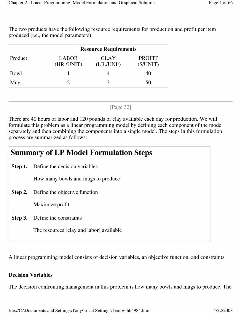
The two products have the following resource requirements for production and profit per item produced (i.e., the model parameters):
[Page 32]
There are 40 hours of labor and 120 pounds of clay available each day for production. We will formulate this problem as a linear programming model by defining each component of the model separately and then combining the components into a single model. The steps in this formulation process are summarized as follows:
A linear programming model consists of decision variables, an objective function, and constraints.
Decision Variables
The decision confronting management in this problem is how many bowls and mugs to produce. The
Resource Requirements
Product LABOR (HR./UNIT)
CLAY (LB./UNIt)
PROFIT ($/UNIT)
Bowl 1 4 40
Mug 2 3 50
Summary of LP Model Formulation Steps
Step 1. Define the decision variables How many bowls and mugs to produce
Step 2. Define the objective function Maximize profit
Step 3. Define the constraints The resources (clay and labor) available
Page 4 of 66Chapter 2. Linear Programming: Model Formulation and Graphical Solution
4/22/2008file://C:\Documents and Settings\Tony\Local Settings\Temp\~hh4984.htm

two decision variables represent the number of bowls and mugs to be produced on a daily basis. The quantities to be produced can be represented symbolically as
x1 = number of bowls to produce
x2 = number of mugs to produce
The Objective Function
The objective of the company is to maximize total profit. The company's profit is the sum of the individual profits gained from each bowl and mug. Profit derived from bowls is determined by multiplying the unit profit of each bowl, $40, by the number of bowls produced, x
1. Likewise, profit
derived from mugs is derived from the unit profit of a mug, $50, multiplied by the number of mugs produced, x
2. Thus, total profit, which we will define symbolically as Z, can be expressed
mathematically as $40x1 + $50x
2. By placing the term maximize in front of the profit function, we
express the objective of the firmto maximize total profit:
maximize Z = $40x1 + 50x
2
where
Model Constraints
In this problem two resources are used for productionlabor and clayboth of which are limited. Production of bowls and mugs requires both labor and clay. For each bowl produced, 1 hour of labor is required. Therefore, the labor used for the production of bowls is 1x
1 hours. Similarly, each mug
requires 2 hours of labor; thus, the labor used to produce mugs every day is 2x2 hours. The total
labor used by the company is the sum of the individual amounts of labor used for each product:
1x1 + 2x
2
[Page 33]
Z = total profit per day
$40x1 = profit from bowls
$50x2 = profit from mugs
Page 5 of 66Chapter 2. Linear Programming: Model Formulation and Graphical Solution
4/22/2008file://C:\Documents and Settings\Tony\Local Settings\Temp\~hh4984.htm

However, the amount of labor represented by 1x1 + 2x
2 is limited to 40 hours per day; thus, the
complete labor constraint is
1x1 + 2x
2 40 hr.
The "less than or equal to" ( ) inequality is employed instead of an equality (=) because the 40 hours of labor is a maximum limitation that can be used, not an amount that must be used. This constraint allows the company some flexibility; the company is not restricted to using exactly 40 hours but can use whatever amount is necessary to maximize profit, up to and including 40 hours. This means that it is possible to have idle, or excess, capacity (i.e., some of the 40 hours may not be used).
The constraint for clay is formulated in the same way as the labor constraint. Because each bowl requires 4 pounds of clay, the amount of clay used daily for the production of bowls is 4x
1 pounds;
and because each mug requires 3 pounds of clay, the amount of clay used daily for mugs is 3x2.
Given that the amount of clay available for production each day is 120 pounds, the material constraint can be formulated as
4x1 + 3x
2 120 lb.
A final restriction is that the number of bowls and mugs produced must be either zero or a positive value because it is impossible to produce negative items. These restrictions are referred to as nonnegativity constraints and are expressed mathematically as
Nonnegativity constraints restrict the decision variables to zero or positive values.
x1 0, x
2 0
The complete linear programming model for this problem can now be summarized as follows:
The solution of this model will result in numeric values for x1 and x
2 that will maximize total profit,
Z. As one possible solution, consider x1 = 5 bowls and x
2 = 10 mugs. First, we will substitute this
Page 6 of 66Chapter 2. Linear Programming: Model Formulation and Graphical Solution
4/22/2008file://C:\Documents and Settings\Tony\Local Settings\Temp\~hh4984.htm

hypothetical solution into each of the constraints in order to make sure that the solution does not require more resources than the constraints show are available:
and
Because neither of the constraints is violated by this hypothetical solution, we say the solution is feasible (i.e., it is possible). Substituting these solution values in the objective function gives Z = 40(5) + 50(10) = $700. However, for the time being, we do not have any way of knowing whether $700 is the maximum profit.
A feasible solution does not violate any of the constraints.
Now consider a solution of x
1 = 10 bowls and x
2 = 20 mugs. This solution results in a profit of
[Page 34]
Although this is certainly a better solution in terms of profit, it is infeasible (i.e., not possible) because it violates the resource constraint for labor:
An infeasible problem violates at least one of the constraints.
The solution to this problem must maximize profit without violating the constraints. The solution that achieves this objective is x
1 = 24 bowls and x
2 = 8 mugs, with a corresponding profit of $1,360.
The determination of this solution is shown using the graphical solution approach in the following section.
[Page 34 (continued)]
Page 7 of 66Chapter 2. Linear Programming: Model Formulation and Graphical Solution
4/22/2008file://C:\Documents and Settings\Tony\Local Settings\Temp\~hh4984.htm

Graphical Solutions of Linear Programming Models
Following the formulation of a mathematical model, the next stage in the application of linear programming to a decision-making problem is to find the solution of the model. A common solution approach is to solve algebraically the set of mathematical relationships that form the model either manually or using a computer program, thus determining the values for the decision variables. However, because the relationships are linear, some models and solutions can be illustrated graphically.
Graphical solutions are limited to linear programming problems with only two decision variables.
The graphical method is realistically limited to models with only two decision variables, which can be represented on a graph of two dimensions. Models with three decision variables can be graphed in three dimensions, but the process is quite cumbersome, and models of four or more decision variables cannot be graphed at all.
Although the graphical method is limited as a solution approach, it is very useful at this point in our presentation of linear programming in that it gives a picture of how a solution is derived. Graphs can provide a clearer understanding of how the computer and mathematical solution approaches presented in subsequent chapters work and, thus, a better understanding of the solutions.
The graphical method provides a picture of how a solution is obtained for a linear programming problem.
Graphical Solution of a Maximization Model
The product mix model will be used to demonstrate the graphical interpretation of a linear programming problem. Recall that the problem describes Beaver Creek Pottery Company's attempt to decide how many bowls and mugs to produce daily, given limited amounts of labor and clay. The complete linear programming model was formulated as
maximize Z = $40x1 + 50x
2
subject to
where
x1 = number of bowls produced
Page 8 of 66Chapter 2. Linear Programming: Model Formulation and Graphical Solution
4/22/2008file://C:\Documents and Settings\Tony\Local Settings\Temp\~hh4984.htm

x2 = number of mugs produced
Figure 2.2 is a set of coordinates for the decision variables x1 and x
2, on which the graph of our
model will be drawn. Note that only the positive quadrant is drawn (i.e., the quadrant where x1 and
x2 will always be positive) because of the nonnegativity constraints, x
1 0 and x
2 0.
[Page 35]
Management Science Application: Operational Cost Control at Kellogg
Kellogg is the world's largest cereal producer and a leading producer of convenience foods, with worldwide sales in 1999 of almost $7 billion. The company started with a single product, Kellogg's Corn Flakes, in 1906 and over the years developed a product line of other cereals, including Rice Krispies and Corn Pops, and convenience foods such as Pop-Tarts and Nutri-Grain cereal bars. Kellogg operates 5 plants in the United States and Canada and 7 distribution centers, and it contracts with 15 co-packers to produce or pack some of the Kellogg products. Kellogg must coordinate the production, packaging, inventory, and distribution of roughly 80 cereal products alone at these various facilities.
For more than a decade Kellogg has been using a large-scale linear programming model called the Kellogg Planning System (KPS) to plan its weekly production, inventory, and distribution decisions. The model decision variables include the amount of each product produced in a production process at each plant, the units of product packaged, the amount of inventory held, and the shipments of products to other plants and distribution centers. Model constraints include production processing time, packaging capacity, balancing constraints that make sure that all products produced are also packaged during the week, inventory balancing constraints, and inventory safety stock requirements. The model objective is cost minimization. Kellogg has also developed a tactical version of this basic operational linear programming model for long-range planning for 12 to 24 months into the future. The KPS model is credited with saving Kellogg $4.5 million in reduced production, inventory, and distribution costs in 1995, and it is estimated that KPS has saved Kellogg many more millions of dollars since the mid-1990s. The tactical version of KPS recently helped the company consolidate production capacity with estimated projected savings of almost $40 million.
Page 9 of 66Chapter 2. Linear Programming: Model Formulation and Graphical Solution
4/22/2008file://C:\Documents and Settings\Tony\Local Settings\Temp\~hh4984.htm
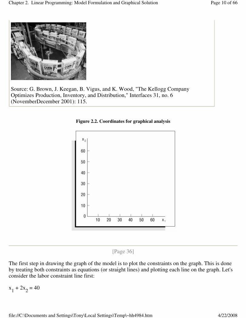
Figure 2.2. Coordinates for graphical analysis
[Page 36]
The first step in drawing the graph of the model is to plot the constraints on the graph. This is done by treating both constraints as equations (or straight lines) and plotting each line on the graph. Let's consider the labor constraint line first:
x1 + 2x
2 = 40
Source: G. Brown, J. Keegan, B. Vigus, and K. Wood, "The Kellogg Company Optimizes Production, Inventory, and Distribution," Interfaces 31, no. 6 (NovemberDecember 2001): 115.
Page 10 of 66Chapter 2. Linear Programming: Model Formulation and Graphical Solution
4/22/2008file://C:\Documents and Settings\Tony\Local Settings\Temp\~hh4984.htm

Constraint lines are plotted as equations.
A simple procedure for plotting this line is to determine two points that are on the line and then draw a straight line through the points. One point can be found by letting x
1 = 0 and solving for x
2:
Thus, one point is at the coordinates x1 = 0 and x
2 = 20. A second point can be found by letting x
2 =
0 and solving for x1:
Now we have a second point, x1 = 40, x
2 = 0. The line on the graph representing this equation is
drawn by connecting these two points, as shown in Figure 2.3. However, this is only the graph of the constraint line and does not reflect the entire constraint, which also includes the values that are less
than or equal to ( ) this line. The area representing the entire constraint is shown in Figure 2.4.
Figure 2.3. Graph of the labor constraint line
To test the correctness of the constraint area, we check any two pointsone inside the constraint area and one outside. For example, check point A in Figure 2.4, which is at the intersection of x
1 = 10 and
Page 11 of 66Chapter 2. Linear Programming: Model Formulation and Graphical Solution
4/22/2008file://C:\Documents and Settings\Tony\Local Settings\Temp\~hh4984.htm

x2 = 10. Substituting these values into the following labor constraint,
[Page 37]
shows that point A is indeed within the constraint area, as these values for x1 and x
2 yield a quantity
that does not exceed the limit of 40 hours. Next, we check point B at x1 = 40 and x
2 = 30:
Figure 2.4. The labor constraint area
Point B is obviously outside the constraint area because the values for x
1 and x
2 yield a quantity
(100) that exceeds the limit of 40 hours.
We draw the line for the clay constraint the same way as the one for the labor constraintby finding two points on the constraint line and connecting them with a straight line. First, let x
1 = 0 and solve
for x2:
Page 12 of 66Chapter 2. Linear Programming: Model Formulation and Graphical Solution
4/22/2008file://C:\Documents and Settings\Tony\Local Settings\Temp\~hh4984.htm

Performing this operation results in a point, x1 = 0, x
2 = 40. Next, we let x
2 = 0 and then solve for
x1:
This operation yields a second point, x1 = 30, x
2 = 0. Plotting these points on the graph and
connecting them with a line gives the constraint line and area for clay, as shown in Figure 2.5.
Figure 2.5. The constraint area for clay (This item is displayed on page 38 in the print version)
Combining the two individual graphs for both labor and clay (Figures 2.4 and 2.5) produces a graph of the model constraints, as shown in Figure 2.6. The shaded area in Figure 2.6 is the area that is common to both model constraints. Therefore, this is the only area on the graph that contains points (i.e., values for x
1 and x
2) that will satisfy both constraints simultaneously. For example, consider
the points R, S, and T in Figure 2.7. Point R satisfies both constraints; thus, we say it is a feasible
solution point. Point S satisfies the clay constraint (4x1 + 3x
2 120) but exceeds the labor
constraint; thus, it is infeasible. Point T satisfies neither constraint; thus, it is also infeasible.
[Page 38]
Figure 2.6. Graph of both model constraints
Page 13 of 66Chapter 2. Linear Programming: Model Formulation and Graphical Solution
4/22/2008file://C:\Documents and Settings\Tony\Local Settings\Temp\~hh4984.htm
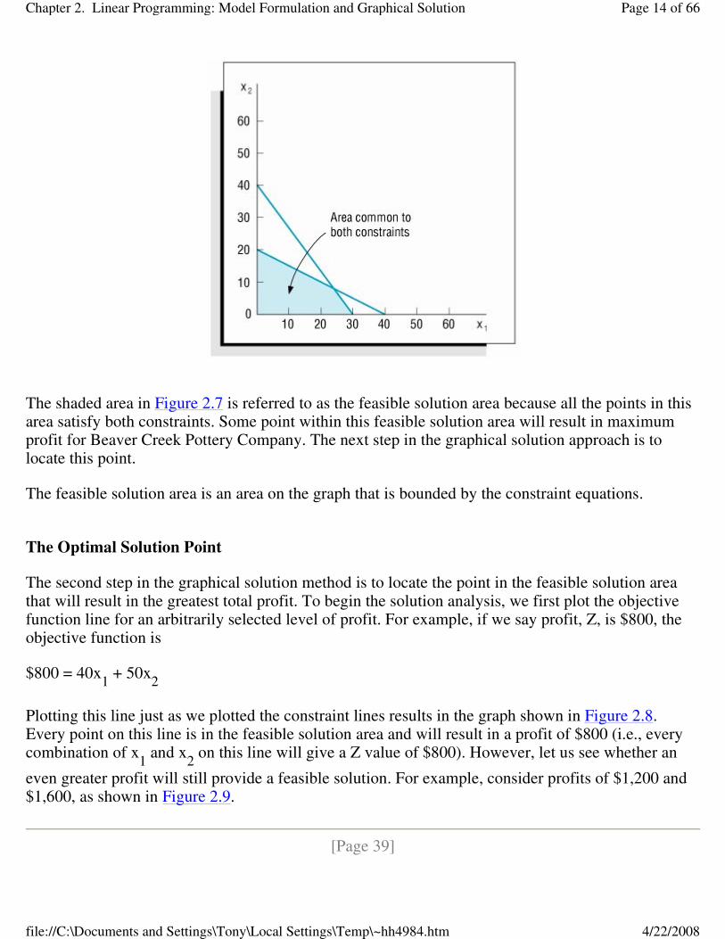
The shaded area in Figure 2.7 is referred to as the feasible solution area because all the points in this area satisfy both constraints. Some point within this feasible solution area will result in maximum profit for Beaver Creek Pottery Company. The next step in the graphical solution approach is to locate this point.
The feasible solution area is an area on the graph that is bounded by the constraint equations.
The Optimal Solution Point
The second step in the graphical solution method is to locate the point in the feasible solution area that will result in the greatest total profit. To begin the solution analysis, we first plot the objective function line for an arbitrarily selected level of profit. For example, if we say profit, Z, is $800, the objective function is
$800 = 40x1 + 50x
2
Plotting this line just as we plotted the constraint lines results in the graph shown in Figure 2.8. Every point on this line is in the feasible solution area and will result in a profit of $800 (i.e., every combination of x
1 and x
2 on this line will give a Z value of $800). However, let us see whether an
even greater profit will still provide a feasible solution. For example, consider profits of $1,200 and $1,600, as shown in Figure 2.9.
[Page 39]
Page 14 of 66Chapter 2. Linear Programming: Model Formulation and Graphical Solution
4/22/2008file://C:\Documents and Settings\Tony\Local Settings\Temp\~hh4984.htm

Figure 2.7. The feasible solution area constraints
Figure 2.8. Objective function line for Z = $800
A portion of the objective function line for a profit of $1,200 is outside the feasible solution area, but part of the line remains within the feasible area. Therefore, this profit line indicates that there are
Page 15 of 66Chapter 2. Linear Programming: Model Formulation and Graphical Solution
4/22/2008file://C:\Documents and Settings\Tony\Local Settings\Temp\~hh4984.htm

feasible solution points that give a profit greater than $800. Now let us increase profit again, to $1,600. This profit line, also shown in Figure 2.9, is completely outside the feasible solution area. The fact that no points on this line are feasible indicates that a profit of $1,600 is not possible.
Because a profit of $1,600 is too great for the constraint limitations, as shown in Figure 2.9, the question of the maximum profit value remains. We can see from Figure 2.9 that profit increases as the objective function line moves away from the origin (i.e., the point x
1 = 0, x
2 = 0). Given this
characteristic, the maximum profit will be attained at the point where the objective function line is farthest from the origin and is still touching a point in the feasible solution area. This point is shown as point B in Figure 2.10.
[Page 40]
Figure 2.9. Alternative objective function lines for profits, Z, of $800, $1,200, and $1,600
Figure 2.10. Identification of optimal solution point
Page 16 of 66Chapter 2. Linear Programming: Model Formulation and Graphical Solution
4/22/2008file://C:\Documents and Settings\Tony\Local Settings\Temp\~hh4984.htm

To find point B, we place a straightedge parallel to the objective function line $800 = 40x
1 + 50x
2 in
Figure 2.10 and move it outward from the origin as far as we can without losing contact with the feasible solution area. Point B is referred to as the optimal (i.e., best) solution.
The optimal solution is the best feasible solution.
The Solution Values
The third step in the graphical solution approach is to solve for the values of x1 and x
2 once the
optimal solution point has been found. It is possible to determine the x1 and x
2 coordinates of point
B in Figure 2.10 directly from the graph, as shown in Figure 2.11. The graphical coordinates corresponding to point B in Figure 2.11 are x
1 = 24 and x
2 = 8. This is the optimal solution for the
decision variables in the problem. However, unless an absolutely accurate graph is drawn, it is frequently difficult to determine the correct solution directly from the graph. A more exact approach is to determine the solution values mathematically once the optimal point on the graph has been determined. The mathematical approach for determining the solution is described in the following pages. First, however, we will consider a few characteristics of the solution.
[Page 41]
Figure 2.11. Optimal solution coordinates
Page 17 of 66Chapter 2. Linear Programming: Model Formulation and Graphical Solution
4/22/2008file://C:\Documents and Settings\Tony\Local Settings\Temp\~hh4984.htm

In Figure 2.10, as the objective function was increased, the last point it touched in the feasible solution area was on the boundary of the feasible solution area. The solution point is always on this boundary because the boundary contains the points farthest from the origin (i.e., the points corresponding to the greatest profit). This characteristic of linear programming problems reduces the number of possible solution points considerably, from all points in the solution area to just those points on the boundary. However, the number of possible solution points is reduced even more by another characteristic of linear programming problems.
The optimal solution point is the last point the objective function touches as it leaves the feasible solution area.
The solution point will be on the boundary of the feasible solution area and at one of the corners of the boundary where two constraint lines intersect. (The graphical axes, you will recall, are also
constraints because x1 0 and x
2 0.) These corners (points A, B, and C in Figure 2.11) are
protrusions, or extremes, in the feasible solution area; they are called extreme points. It has been proven mathematically that the optimal solution in a linear programming model will always occur at an extreme point. Therefore, in our sample problem the possible solution points are limited to the three extreme points, A, B, and C. The optimal extreme point is the extreme point the objective function touches last as it leaves the feasible solution area, as shown in Figure 2.10.
Extreme points are corner points on the boundary of the feasible solution area.
Page 18 of 66Chapter 2. Linear Programming: Model Formulation and Graphical Solution
4/22/2008file://C:\Documents and Settings\Tony\Local Settings\Temp\~hh4984.htm

From the graph shown in Figure 2.10, we know that the optimal solution point is B. Because point B is formed by the intersection of two constraint lines, as shown in Figure 2.11, these two lines are equal at point B. Thus, the values of x
1 and x
2 at that intersection can be found by solving the two
equations simultaneously.
Constraint equations are solved simultaneously at the optimal extreme point to determine the variable solution values.
First, we convert both equations to functions of x
1:
and
[Page 42]
Now we let x1 in the first equation equal x
1 in the second equation,
40 2x2 = 30 (3x
2/4)
and solve for x2:
Substituting x2 = 8 into either one of the original equations gives a value for x
1:
Thus, the optimal solution at point B in Figure 2.11 is x1 = 24 and x
2 = 8. Substituting these values
into the objective function gives the maximum profit,
Page 19 of 66Chapter 2. Linear Programming: Model Formulation and Graphical Solution
4/22/2008file://C:\Documents and Settings\Tony\Local Settings\Temp\~hh4984.htm

In terms of the original problem, the solution indicates that if the pottery company produces 24 bowls and 8 mugs, it will receive $1,360, the maximum daily profit possible (given the resource constraints).
Given that the optimal solution will be at one of the extreme corner points, A, B, or C, we can also find the solution by testing each of the three points to see which results in the greatest profit, rather than by graphing the objective function and seeing which point it last touches as it moves out of the feasible solution area. Figure 2.12 shows the solution values for all three points, A, B, and C, and the amount of profit, Z, at each point.
Figure 2.12. Solutions at all corner points
As indicated in the discussion of Figure 2.10, point B is the optimal solution point because it is the last point the objective function touches before it leaves the solution area. In other words, the objective function determines which extreme point is optimal. This is because the objective function designates the profit that will accrue from each combination of x
1 and x
2 values at the extreme
points. If the objective function had had different coefficients (i.e., different x1 and x
2 profit values),
one of the extreme points other than B might have been optimal.
[Page 43]
Let's assume for a moment that the profit for a bowl is $70 instead of $40, and the profit for a mug is $20 instead of $50. These values result in a new objective function, Z = $70x
1 + 20x
2. If the model
Page 20 of 66Chapter 2. Linear Programming: Model Formulation and Graphical Solution
4/22/2008file://C:\Documents and Settings\Tony\Local Settings\Temp\~hh4984.htm

constraints for labor or clay are not changed, the feasible solution area remains the same, as shown in Figure 2.13. However, the location of the objective function in Figure 2.13 is different from that of the original objective function in Figure 2.10. The reason for this change is that the new profit coefficients give the linear objective function a new slope.
Figure 2.13. The optimal solution with Z = 70x1 + 20x
2
The slope can be determined by transforming the objective function into the general equation for a straight line, y = a + bx, where y is the dependent variable, a is the y intercept, b is the slope, and x is the independent variable. For our sample objective function, x
2 is the dependent variable
corresponding to y (i.e., it is on the vertical axis), and x1 is the independent variable. Thus, the
objective function can be transformed into the general equation of a line as follows:
The slope is computed as the "rise" over the "run."
This transformation identifies the slope of the new objective function as 7/2 (the minus sign indicates
Page 21 of 66Chapter 2. Linear Programming: Model Formulation and Graphical Solution
4/22/2008file://C:\Documents and Settings\Tony\Local Settings\Temp\~hh4984.htm

that the line slopes downward). In contrast, the slope of the original objective function was 4/5.
If we move this new objective function out through the feasible solution area, the last extreme point it touches is point C. Simultaneously solving the constraint lines at point C results in the following solution:
and
Thus, the optimal solution at point C in Figure 2.13 is x1 = 30 bowls, x
2 = 0 mugs, and Z = $2,100
profit. Altering the objective function coefficients results in a new solution.
[Page 44]
This brief example of the effects of altering the objective function highlights two useful points. First, the optimal extreme point is determined by the objective function, and an extreme point on one axis of the graph is as likely to be the optimal solution as is an extreme point on a different axis. Second, the solution is sensitive to the values of the coefficients in the objective function. If the objective function coefficients are changed, as in our example, the solution may change. Likewise, if the constraint coefficients are changed, the solution space and solution points may change also. This information can be of consequence to the decision maker trying to determine how much of a product to produce. Sensitivity analysisthe use of linear programming to evaluate the effects of changes in model parametersis discussed in Chapter 3.
Sensitivity analysis is used to analyze changes in model parameters.
It should be noted that some problems do not have a single extreme point solution. For example, when the objective function line parallels one of the constraint lines, an entire line segment is bounded by two adjacent corner points that are optimal; there is no single extreme point on the objective function line. In this situation there are multiple optimal solutions. This and other irregular types of solution outcomes in linear programming are discussed at the end of this chapter.
Multiple optimal solutions can occur when the objective function is parallel to a constraint line.
Slack Variables
Page 22 of 66Chapter 2. Linear Programming: Model Formulation and Graphical Solution
4/22/2008file://C:\Documents and Settings\Tony\Local Settings\Temp\~hh4984.htm

Once the optimal solution was found at point B in Figure 2.12, simultaneous equations were solved to determine the values of x
1 and x
2. Recall that the solution occurs at an extreme point where
constraint equation lines intersect with each other or with the axis. Thus, the model constraints are
considered as equations (=) rather than or inequalities.
There is a standard procedure for transforming inequality constraints into equations. This transformation is achieved by adding a new variable, called a slack variable, to each constraint. For the pottery company example, the model constraints are
x1 + 2x
2 40 hr. of labor
4x1 + 3x
2 120 lb. of clay
A slack variable is added to a constraint to convert it to an equation (=).
The addition of a unique slack variable, s
1, to the labor constraint and s
2 to the constraint for clay
results in the following equations:
x1 + 2x
2 + s
1 = 40 hr. of labor
4x1 + 3x
2 + s
2 = 120 lb. of clay
A slack variable represents unused resources.
The slack variables in these equations, s
1 and s
2, will take on any value necessary to make the left-
hand side of the equation equal to the right-hand side. For example, consider a hypothetical solution of x
1 = 5 and x
2 = 10. Substituting these values into the foregoing equations yields
and
Page 23 of 66Chapter 2. Linear Programming: Model Formulation and Graphical Solution
4/22/2008file://C:\Documents and Settings\Tony\Local Settings\Temp\~hh4984.htm

In this example, x1 = 5 bowls and x
2 = 10 mugs represent a solution that does not make use of the
total available amount of labor and clay. In the labor constraint, 5 bowls and 10 mugs require only 25 hours of labor. This leaves 15 hours that are not used. Thus, s
1 represents the amount of unused
labor, or slack.
[Page 45]
In the clay constraint, 5 bowls and 10 mugs require only 50 pounds of clay. This leaves 70 pounds of clay unused. Thus, s
2 represents the amount of unused clay. In general, slack variables represent the
amount of unused resources.
The ultimate instance of unused resources occurs at the origin, where x1 = 0 and x
2 = 0. Substituting
these values into the equations yields
and
Because no production takes place at the origin, all the resources are unused; thus, the slack variables equal the total available amounts of each resource: s
1 = 40 hours of labor and s
2 = 120 pounds of
clay.
What is the effect of these new slack variables on the objective function? The objective function for our example represents the profit gained from the production of bowls and mugs,
Z = $40x1 + $50x
2
The coefficient $40 is the contribution to profit of each bowl; $50 is the contribution to profit of each mug. What, then, do the slack variables s
1 and s
2 contribute? They contribute nothing to profit
because they represent unused resources. Profit is made only after the resources are put to use in making bowls and mugs. Using slack variables, we can write the objective function as
A slack variable contributes nothing to the objective function value.
maximize Z = $40x
1 + $50x
2 + 0s
1 + 0s
2
Page 24 of 66Chapter 2. Linear Programming: Model Formulation and Graphical Solution
4/22/2008file://C:\Documents and Settings\Tony\Local Settings\Temp\~hh4984.htm
As in the case of decision variables (x1 and x
2), slack variables can have only nonnegative values
because negative resources are not possible. Therefore, for this model formulation, x1, x
2, s
1, and s
2
0.
The complete linear programming model can be written in what is referred to as standard form with slack variables as follows:
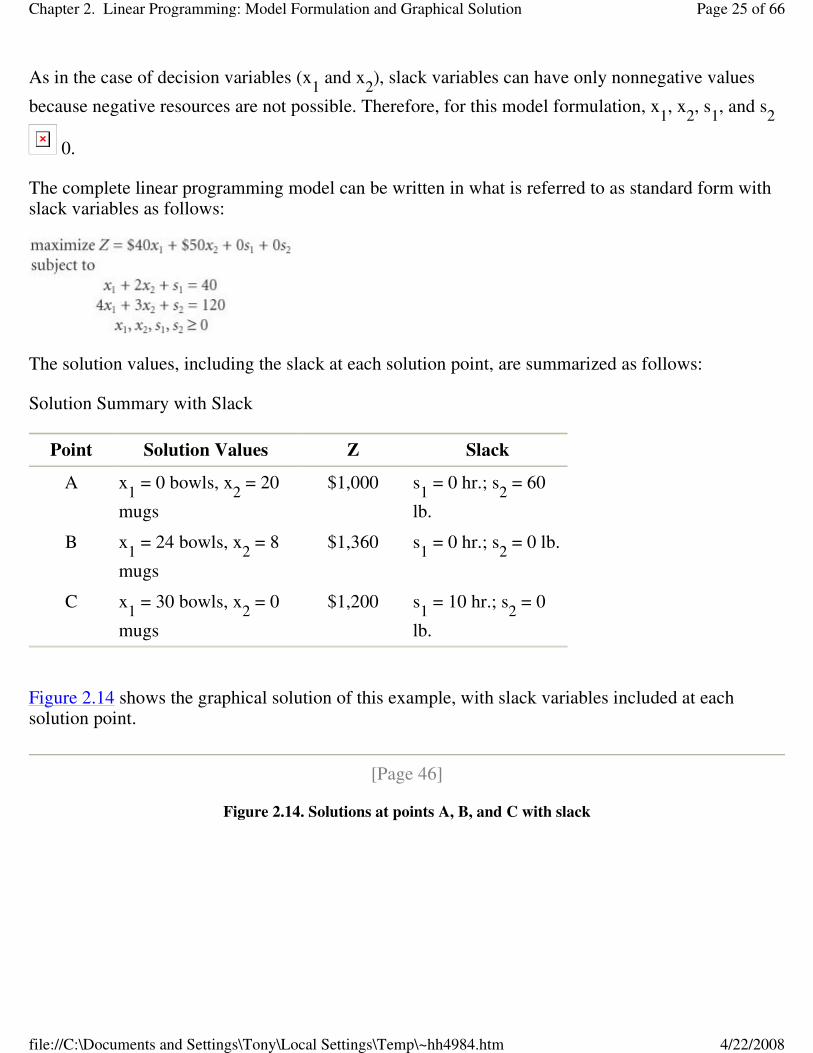
The solution values, including the slack at each solution point, are summarized as follows:
Solution Summary with Slack
Figure 2.14 shows the graphical solution of this example, with slack variables included at each solution point.
[Page 46]
Figure 2.14. Solutions at points A, B, and C with slack
Point Solution Values Z Slack
A x1 = 0 bowls, x
2 = 20
mugs
$1,000 s1 = 0 hr.; s
2 = 60
lb.
B x1 = 24 bowls, x
2 = 8
mugs
$1,360 s1 = 0 hr.; s
2 = 0 lb.
C x1 = 30 bowls, x
2 = 0
mugs
$1,200 s1 = 10 hr.; s
2 = 0
lb.
Page 25 of 66Chapter 2. Linear Programming: Model Formulation and Graphical Solution
4/22/2008file://C:\Documents and Settings\Tony\Local Settings\Temp\~hh4984.htm

Management Science Application: Estimating Food Nutrient Values at Minnesota's Nutrition Coordinating Center
The Nutrition Coordinating Center (NCC) at the University of Minnesota maintains a food composition database used by institutions around the world. This database is used to calculate dietary material intake; to plan menus; to explore the relationships between diet and disease; to meet regulatory requirements; and to monitor the effects of education, intervention, and regulation. These calculations require an enormous amount of nutrient value data for different food products.
Every year, more than 12,000 new brand-name food products are introduced into the marketplace. However, it's not feasible to perform a chemical analysis on all foods for multiple nutrients, and so the NCC estimates thousands of nutrient values each year. The NCC has used a time-consuming trial-and-error approach to estimating these nutrient values. These estimates are a composite of the foods already in the database. The NCC developed a linear programming model that determines ingredient amounts in new food products. These estimated ingredient amounts are subsequently used to calculate nutrient amounts for a food product. The nutritionist normally uses the linear programming model to derive an initial estimate of ingredient amounts and then fine-tunes these amounts. The model has reduced the average time it takes to estimate a product formula from 8.3 minutes (using the trial-and-error approach) to 2.1 minutes of labor time and
Page 26 of 66Chapter 2. Linear Programming: Model Formulation and Graphical Solution
4/22/2008file://C:\Documents and Settings\Tony\Local Settings\Temp\~hh4984.htm

Summary of the Graphical Solution Steps
The steps for solving a graphical linear programming model are summarized here:
Or
effort.
Source: B. J. Westrich, M. A. Altmann, and S. J. Potthoff, "Minnesota's Nutrition Coordinating Center Uses Mathematical Optimization to Estimate Food Nutrient Values," Interfaces 28, no. 5 (SeptemberOctober 1998): 8699.
1. Plot the model constraints as equations on the graph; then, considering the inequalities of the constraints, indicate the feasible solution area.
[Page 47]
2. Plot the objective function; then move this line out from the origin to locate the optimal solution point.
3. Solve simultaneous equations at the solution point to find the optimal solution values.
2. Solve simultaneous equations at each corner point to find the solution values at each point.
3. Substitute these values into the objective function to find the set of values that results in the maximum Z value.
Page 27 of 66Chapter 2. Linear Programming: Model Formulation and Graphical Solution
4/22/2008file://C:\Documents and Settings\Tony\Local Settings\Temp\~hh4984.htm

[Page 47 (continued)]
A Minimization Model Example
As mentioned at the beginning of this chapter, there are two types of linear programming problems: maximization problems (like the Beaver Creek Pottery Company example) and minimization problems. A minimization problem is formulated the same basic way as a maximization problem, except for a few minor differences. The following sample problem will demonstrate the formulation of a minimization model.
A farmer is preparing to plant a crop in the spring and needs to fertilize a field. There are two brands of fertilizer to choose from, Super-gro and Crop-quick. Each brand yields a specific amount of nitrogen and phosphate per bag, as follows:
The farmer's field requires at least 16 pounds of nitrogen and 24 pounds of phosphate. Super-gro costs $6 per bag, and Crop-quick costs $3. The farmer wants to know how many bags of each brand to purchase in order to minimize the total cost of fertilizing. This scenario is illustrated in Figure 2.15.
The steps in the linear programming model formulation process are summarized as follows:
Chemical Contribution
Brand NITROGEN (LB./BAG)
PHOSPHATE (LB./BAG)
Super-gro 2 4
Crop-quick 4 3
Summary of LP Model Formulation Steps
Step 1. Define the decision variables How many bags of Super-gro and Crop-quick to buy
Step 2. Define the objective function Minimize cost
Step 3. Define the constraints
Page 28 of 66Chapter 2. Linear Programming: Model Formulation and Graphical Solution
4/22/2008file://C:\Documents and Settings\Tony\Local Settings\Temp\~hh4984.htm

Decision Variables
This problem contains two decision variables, representing the number of bags of each brand of fertilizer to purchase:
x1 = bags of Super-gro
x2 = bags of Crop-quick
[Page 48]
Figure 2.15. Fertilizing farmer's field
[View full size image]
The field requirements for nitrogen and phosphate
Page 29 of 66Chapter 2. Linear Programming: Model Formulation and Graphical Solution
4/22/2008file://C:\Documents and Settings\Tony\Local Settings\Temp\~hh4984.htm

The Objective Function
The farmer's objective is to minimize the total cost of fertilizing. The total cost is the sum of the individual costs of each type of fertilizer purchased. The objective function that represents total cost is expressed as
minimize Z = $6x1 + 3x
2
where
$6x1 = cost of bags of Super-gro
$3x2 = cost of bags of Crop-quick
Model Constraints
The requirements for nitrogen and phosphate represent the constraints of the model. Each bag of fertilizer contributes a number of pounds of nitrogen and phosphate to the field. The constraint for nitrogen is
2x1 + 4x
2 16 lb.
where
2x1 = the nitrogen contribution (lb.) per bag of Super-gro
4x2 = the nitrogen contribution (lb.) per bag of Crop-quick
Rather than a (less than or equal to) inequality, as used in the Beaver Creek Pottery Company
model, this constraint requires a (greater than or equal to) inequality. This is because the nitrogen content for the field is a minimum requirement specifying that at least 16 pounds of nitrogen be deposited on the farmer's field. If a minimum cost solution results in more than 16 pounds of nitrogen on the field, that is acceptable; however, the amount cannot be less than 16 pounds.
[Page 49]
The constraint for phosphate is constructed like the constraint for nitrogen:
4x1 + 3x
2 24 lb.
Page 30 of 66Chapter 2. Linear Programming: Model Formulation and Graphical Solution
4/22/2008file://C:\Documents and Settings\Tony\Local Settings\Temp\~hh4984.htm

With this example we have shown two of the three types of linear programming model constraints,
and . The third type is an exact equality, =. This type specifies that a constraint requirement must be exact. For example, if the farmer had said that the phosphate requirement for the field was exactly 24 pounds, the constraint would have been
The three types of linear programming constraints are , =, and .
4x
1 + 3x
2 = 24 lb.
As in our maximization model, there are also nonnegativity constraints in this problem to indicate that negative bags of fertilizer cannot be purchased:
x1, x
2 0
The complete model formulation for this minimization problem is
Graphical Solution of a Minimization Model
We follow the same basic steps in the graphical solution of a minimization model as in a maximization model. The fertilizer example will be used to demonstrate the graphical solution of a minimization model.
The first step is to graph the equations of the two model constraints, as shown in Figure 2.16. Next,
the feasible solution area is chosen, to reflect the inequalities in the constraints, as shown in Figure 2.17.
Figure 2.16. Constraint lines for fertilizer model
Page 31 of 66Chapter 2. Linear Programming: Model Formulation and Graphical Solution
4/22/2008file://C:\Documents and Settings\Tony\Local Settings\Temp\~hh4984.htm

[Page 50]
Figure 2.17. Feasible solution area
After the feasible solution area has been determined, the second step in the graphical solution approach is to locate the optimal point. Recall that in a maximization problem, the optimal solution is
Page 32 of 66Chapter 2. Linear Programming: Model Formulation and Graphical Solution
4/22/2008file://C:\Documents and Settings\Tony\Local Settings\Temp\~hh4984.htm

on the boundary of the feasible solution area that contains the point(s) farthest from the origin. The optimal solution point in a minimization problem is also on the boundary of the feasible solution area; however, the boundary contains the point(s) closest to the origin (zero being the lowest cost possible).
The optimal solution of a minimization problem is at the extreme point closest to the origin.
As in a maximization problem, the optimal solution is located at one of the extreme points of the boundary. In this case the corner points represent extremities in the boundary of the feasible solution area that are closest to the origin. Figure 2.18 shows the three corner pointsA, B, and Cand the objective function line.
As the objective function edges toward the origin, the last point it touches in the feasible solution area is A. In other words, point A is the closest the objective function can get to the origin without encompassing infeasible points. Thus, it corresponds to the lowest cost that can be attained.
Figure 2.18. The optimal solution point
[Page 51]
Management Science Application: Determining Optimal Fertilizer Mixes at Soquimich (South America)
Page 33 of 66Chapter 2. Linear Programming: Model Formulation and Graphical Solution
4/22/2008file://C:\Documents and Settings\Tony\Local Settings\Temp\~hh4984.htm

The final step in the graphical solution approach is to solve for the values of x
1 and x
2 at point A.
Because point A is on the x2 axis, x
1 = 0; thus,
Given that the optimal solution is x1 = 0, x
2 = 8, the minimum cost, Z, is
Soquimich, a Chilean fertilizer manufacturer, is the leading producer and distributor of specialty fertilizers in the world, with revenues of almost US$0.5 billion in more than 80 countries. Soquimich produces four main specialty fertilizers and more than 200 fertilizer blends, depending on the needs of its customers. Farmers want the company to quickly recommend optimal fertilizer blends that will provide the appropriate quantity of ingredients for their particular crop at the lowest possible cost. A farmer will provide a company sales representative with information about previous crop yields and his or her target yields and then company representatives will visit the farm to obtain soil samples, which are analyzed in the company labs. A report is generated, which indicates the soil requirements for nutrients, including nitrogen, phosphorus, potassium, boron, magnesium, sulfur, and zinc. Given these soil requirements, company experts determine an optimal fertilizer blend, using a linear programming model that includes constraints for the nutrient quantities required by the soil (for a particular crop) and an objective function that minimizes production costs. Previously the company determined fertilizer blend recommendations by using a time-consuming manual procedure conducted by experts. The linear programming model enables the company to provide accurate, quick, low-cost (discounted) estimates to its customers, which has helped the company gain new customers and increase its market share.
Source: A. M. Angel, L. A. Taladriz, and R. Weber. "Soquimich Uses a System Based on Mixed-Integer Linear Programming and Expert Systems to Improve Customer Service," Interfaces 33, no. 4 (JulyAugust 2003): 4152.
Page 34 of 66Chapter 2. Linear Programming: Model Formulation and Graphical Solution
4/22/2008file://C:\Documents and Settings\Tony\Local Settings\Temp\~hh4984.htm

This means the farmer should not purchase any Super-gro but, instead, should purchase eight bags of Crop-quick, at a total cost of $24.
Surplus Variables
Greater than or equal to constraints cannot be converted to equations by adding slack variables, as
with constraints. Recall our fertilizer model, formulated as
[Page 52]
where
x1 = bags of Super-gro fertilizer
x2 = bags of Crop-quick fertilizer
Z = farmer's total cost ($) of purchasing fertilizer
Because this problem has constraints as opposed to the constraints of the Beaver Creek Pottery Company maximization example, the constraints are converted to equations a little differently.
A surplus variable is subtracted from a constraint to convert it to an equation (=).
Instead of adding a slack variable with a constraint, we subtract a surplus variable. Whereas a slack variable is added and reflects unused resources, a surplus variable is subtracted and reflects the excess above a minimum resource requirement level. Like a slack variable, a surplus variable is represented symbolically by s
1 and must be nonnegative.
For the nitrogen constraint, the subtraction of a surplus variable gives
Page 35 of 66Chapter 2. Linear Programming: Model Formulation and Graphical Solution
4/22/2008file://C:\Documents and Settings\Tony\Local Settings\Temp\~hh4984.htm

A surplus variable represents an excess above a constraint requirement level.
2x
1 + 4x
2 s
1 = 16
The surplus variable s1 transforms the nitrogen constraint into an equation.
As an example, consider the hypothetical solution
x1 = 0
x2 = 10
Substituting these values into the previous equation yields
In this equation s1 can be interpreted as the extra amount of nitrogen above the minimum
requirement of 16 pounds that would be obtained by purchasing 10 bags of Crop-quick fertilizer.
In a similar manner, the constraint for phosphate is converted to an equation by subtracting a surplus variable, s
2:
4x1 + 3x
2 s
2 = 24
Figure 2.19. Graph of the fertilizer example
Page 36 of 66Chapter 2. Linear Programming: Model Formulation and Graphical Solution
4/22/2008file://C:\Documents and Settings\Tony\Local Settings\Temp\~hh4984.htm

[Page 53]
As is the case with slack variables, surplus variables contribute nothing to the overall cost of a model. For example, putting additional nitrogen or phosphate on the field will not affect the farmer's cost; the only thing affecting cost is the number of bags of fertilizer purchased. As such, the standard form of this linear programming model is summarized as
Figure 2.19 shows the graphical solutions for our example, with surplus variables included at each solution point.
[Page 53 (continued)]
Irregular Types of Linear Programming Problems
The basic forms of typical maximization and minimization problems have been shown in this
Page 37 of 66Chapter 2. Linear Programming: Model Formulation and Graphical Solution
4/22/2008file://C:\Documents and Settings\Tony\Local Settings\Temp\~hh4984.htm

chapter. However, there are several special types of atypical linear programming problems. Although these special cases do not occur frequently, they will be described so that you can recognize them when they arise. These special types include problems with more than one optimal solution, infeasible problems, and problems with unbounded solutions.
For some linear programming models, the general rules do not always apply.
Multiple Optimal Solutions
Consider the Beaver Creek Pottery Company example, with the objective function changed f rom Z = 40x
1 + 50x
2 to Z = 40x
1 + 30x
2:
where
x1 = bowls produced
x2 = mugs produced
The graph of this model is shown in Figure 2.20. The slight change in the objective function makes it now parallel to the constraint line, 4x
1 + 3x
2 = 120. Both lines now have the same slope of 4/3.
Therefore, as the objective function edge moves outward from the origin, it touches the whole line segment BC rather than a single extreme corner point before it leaves the feasible solution area. This means that every point along this line segment is optimal (i.e., each point results in the same profit of Z = $1,200). The endpoints of this line segment, B and C, are typically referred to as the alternate optimal solutions. It is understood that these points represent the endpoints of a range of optimal solutions.
Alternate optimal solutions are at the endpoints of the constraint line segment that the objective function parallels.
Multiple optimal solutions provide greater flexibility to the decision maker.
The pottery company, therefore, has several options in deciding on the number of bowls and mugs to produce. Multiple optimal solutions can benefit the decision maker because the number of decision options is enlarged. The multiple optimal solutions (along the line segment BC in Figure 2.20) allow
Page 38 of 66Chapter 2. Linear Programming: Model Formulation and Graphical Solution
4/22/2008file://C:\Documents and Settings\Tony\Local Settings\Temp\~hh4984.htm

the decision maker greater flexibility. For example, in the case of Beaver Creek Pottery Company, it may be easier to sell bowls than mugs; thus, the solution at point C, where only bowls are produced, would be more desirable than the solution at point B, where a mix of bowls and mugs is produced.
[Page 54]
Figure 2.20. Graph of the Beaver Creek Pottery Company example with multiple optimal solutions
An Infeasible Problem
In some cases a linear programming problem has no feasible solution area; thus, there is no solution to the problem. An example of an infeasible problem is formulated next and depicted graphically in Figure 2.21:
Figure 2.21. Graph of an infeasible problem
Page 39 of 66Chapter 2. Linear Programming: Model Formulation and Graphical Solution
4/22/2008file://C:\Documents and Settings\Tony\Local Settings\Temp\~hh4984.htm

An infeasible problem has no feasible solution area; every possible solution point violates one or more constraints.
[Page 55]
Point A in Figure 2.21 satisfies only the constraint 4x1 + 2x
2 8, whereas point C satisfies only
the constraints x1 4 and x
2 6. Point B satisfies none of the constraints. The three constraints
do not overlap to form a feasible solution area. Because no point satisfies all three constraints simultaneously, there is no solution to the problem. Infeasible problems do not typically occur, but when they do, they are usually a result of errors in defining the problem or in formulating the linear programming model.
An Unbounded Problem
In some problems the feasible solution area formed by the model constraints is not closed. In these cases it is possible for the objective function to increase indefinitely without ever reaching a maximum value because it never reaches the boundary of the feasible solution area.
In an unbounded problem the objective function can increase indefinitely without reaching a maximum value.
Page 40 of 66Chapter 2. Linear Programming: Model Formulation and Graphical Solution
4/22/2008file://C:\Documents and Settings\Tony\Local Settings\Temp\~hh4984.htm
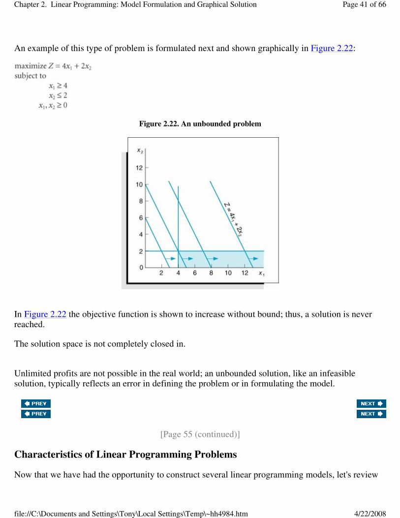
An example of this type of problem is formulated next and shown graphically in Figure 2.22:
Figure 2.22. An unbounded problem
In Figure 2.22 the objective function is shown to increase without bound; thus, a solution is never reached.
The solution space is not completely closed in.
Unlimited profits are not possible in the real world; an unbounded solution, like an infeasible solution, typically reflects an error in defining the problem or in formulating the model.
[Page 55 (continued)]
Characteristics of Linear Programming Problems
Now that we have had the opportunity to construct several linear programming models, let's review
Page 41 of 66Chapter 2. Linear Programming: Model Formulation and Graphical Solution
4/22/2008file://C:\Documents and Settings\Tony\Local Settings\Temp\~hh4984.htm

the characteristics that identify a linear programming problem.
The components of a linear programming model are an objective function, decision variables, and constraints.
A linear programming problem requires a choice between alternative courses of action (i.e., a decision). The decision is represented in the model by decision variables. A typical choice task for a business firm is deciding how much of several different products to produce, as in the Beaver Creek Pottery Company example presented earlier in this chapter. Identifying the choice task and defining the decision variables is usually the first step in the formulation process because it is quite difficult to construct the objective function and constraints without first identifying the decision variables.
[Page 56]
The problem encompasses an objective that the decision maker wants to achieve. The two most frequently encountered objectives for a business are maximizing profit and minimizing cost.
A third characteristic of a linear programming problem is that restrictions exist, making unlimited achievement of the objective function impossible. In a business firm these restrictions often take the form of limited resources, such as labor or material; however, the sample models in this chapter exhibit a variety of problem restrictions. These restrictions, as well as the objective, must be definable by mathematical functional relationships that are linear. Defining these relationships is typically the most difficult part of the formulation process.
Properties of Linear Programming Models
In addition to encompassing only linear relationships, a linear programming model also has several other implicit properties, which have been exhibited consistently throughout the examples in this chapter. The term linear not only means that the functions in the models are graphed as a straight line; it also means that the relationships exhibit proportionality. In other words, the rate of change, or slope, of the function is constant; therefore, changes of a given size in the value of a decision variable will result in exactly the same relative changes in the functional value.
Proportionality means the slope of a constraint or objective function line is constant.
Linear programming also requires that the objective function terms and the constraint terms be additive. For example, in the Beaver Creek Pottery Company model, the total profit (Z) must equal the sum of profits earned from making bowls ($40x
1) and mugs ($50x
2). Also, the total resources
used must equal the sum of the resources used for each activity in a constraint (e.g., labor).
The terms in the objective function or constraints are additive.
Page 42 of 66Chapter 2. Linear Programming: Model Formulation and Graphical Solution
4/22/2008file://C:\Documents and Settings\Tony\Local Settings\Temp\~hh4984.htm

Another property of linear programming models is that the solution values (of the decision variables) cannot be restricted to integer values; the decision variables can take on any fractional value. Thus, the variables are said to be continuous or divisible, as opposed to integer or discrete. For example, although decision variables representing bowls or mugs or airplanes or automobiles should realistically have integer (whole number) solutions, the solution methods for linear programming will not necessarily provide such solutions. This is a property that will be discussed further as solution methods are presented in subsequent chapters.
The values of decision variables are continuous or divisible.
The final property of linear programming models is that the values of all the model parameters are assumed to be constant and known with certainty. In real situations, however, model parameters are frequently uncertain because they reflect the future as well as the present, and future conditions are rarely known with certainty.
All model parameters are assumed to be known with certainty.
To summarize, a linear programming model has the following general properties: linearity, proportionality, additivity, divisibility, and certainty. As various linear programming solution methods are presented throughout this book, these properties will become more obvious, and their impact on problem solution will be discussed in greater detail.
[Page 57]
Summary
The two example problems in this chapter were formulated as linear programming models in order to demonstrate the modeling process. These problems were similar in that they concerned achieving some objective subject to a set of restrictions or requirements. Linear programming models exhibit certain common characteristics:
� An objective function to be maximized or minimized
� A set of constraints
� Decision variables for measuring the level of activity
� Linearity among all constraint relationships and the objective function
Page 43 of 66Chapter 2. Linear Programming: Model Formulation and Graphical Solution
4/22/2008file://C:\Documents and Settings\Tony\Local Settings\Temp\~hh4984.htm

The graphical approach to the solution of linear programming problems is not a very efficient means of solving problems. For one thing, drawing accurate graphs is tedious. Moreover, the graphical approach is limited to models with only two decision variables. However, the analysis of the graphical approach provides valuable insight into linear programming problems and their solutions.
In the graphical approach, once the feasible solution area and the optimal solution point have been determined from the graph, simultaneous equations are solved to determine the values of x
1 and x
2 at
the solution point. In Chapter 3 we will show how linear programming solutions can be obtained using computer programs.
[Page 57 (continued)]
References
Baumol, W. J. Economic Theory and Operations Analysis, 4th ed. Upper Saddle River, NJ: Prentice Hall, 1977.
Charnes, A., and Cooper, W. W. Management Models and Industrial Applications of Linear Programming. New York: John Wiley & Sons, 1961.
Dantzig, G. B. Linear Programming and Extensions. Princeton, NJ: Princeton University Press, 1963.
Gass, S. Linear Programming, 4th ed. New York: McGraw-Hill, 1975.
Hadley, G. Linear Programming. Reading, MA: Addison-Wesley, 1962.
Hillier, F. S., and Lieberman, G. J. Introduction to Operations Research, 4th ed. San Francisco: Holden-Day, 1986.
Llewellyn, R. W. Linear Programming. New York: Holt, Rinehart and Winston, 1964.
Taha, H. A. Operations Research, an Introduction, 4th ed. New York: Macmillan, 1987.
Wagner, H. M. Principles of Operations Research, 2nd ed. Upper Saddle River, NJ: Prentice Hall, 1975.
Page 44 of 66Chapter 2. Linear Programming: Model Formulation and Graphical Solution
4/22/2008file://C:\Documents and Settings\Tony\Local Settings\Temp\~hh4984.htm

[Page 57 (continued)]
Example Problem Solutions
As a prelude to the problems, this section presents example solutions to two linear programming problems.
Problem Statement
Moore's Meatpacking Company produces a hot dog mixture in 1,000-pound batches. The mixture contains two ingredientschicken and beef. The cost per pound of each of these ingredients is as follows:
[Page 58]
Each batch has the following recipe requirements:
a. At least 500 pounds of chicken
b. At least 200 pounds of beef
The ratio of chicken to beef must be at least 2 to 1. The company wants to know the optimal mixture of ingredients that will minimize cost. Formulate a linear programming model for this problem.
Solution
Ingredient Cost/lb.
Chicken $3
Beef $5
Step 1. Identify Decision Variables Recall that the problem should not be "swallowed whole." Identify each part of the model separately, starting with the decision variables: x
1 = lb. of chicken
x
2 = lb. of beef
Step 2. Formulate the Objective Function
Page 45 of 66Chapter 2. Linear Programming: Model Formulation and Graphical Solution
4/22/2008file://C:\Documents and Settings\Tony\Local Settings\Temp\~hh4984.htm

Problem Statement
Solve the following linear programming model graphically:
[Page 59]
Solution
Step 3. Establish Model Constraints
The constraints of this problem are embodied in the recipe restrictions and (not to be overlooked) the fact that each batch must consist of 1,000 pounds of mixture:
and
x1, x
2 0
The Model
Page 46 of 66Chapter 2. Linear Programming: Model Formulation and Graphical Solution
4/22/2008file://C:\Documents and Settings\Tony\Local Settings\Temp\~hh4984.htm
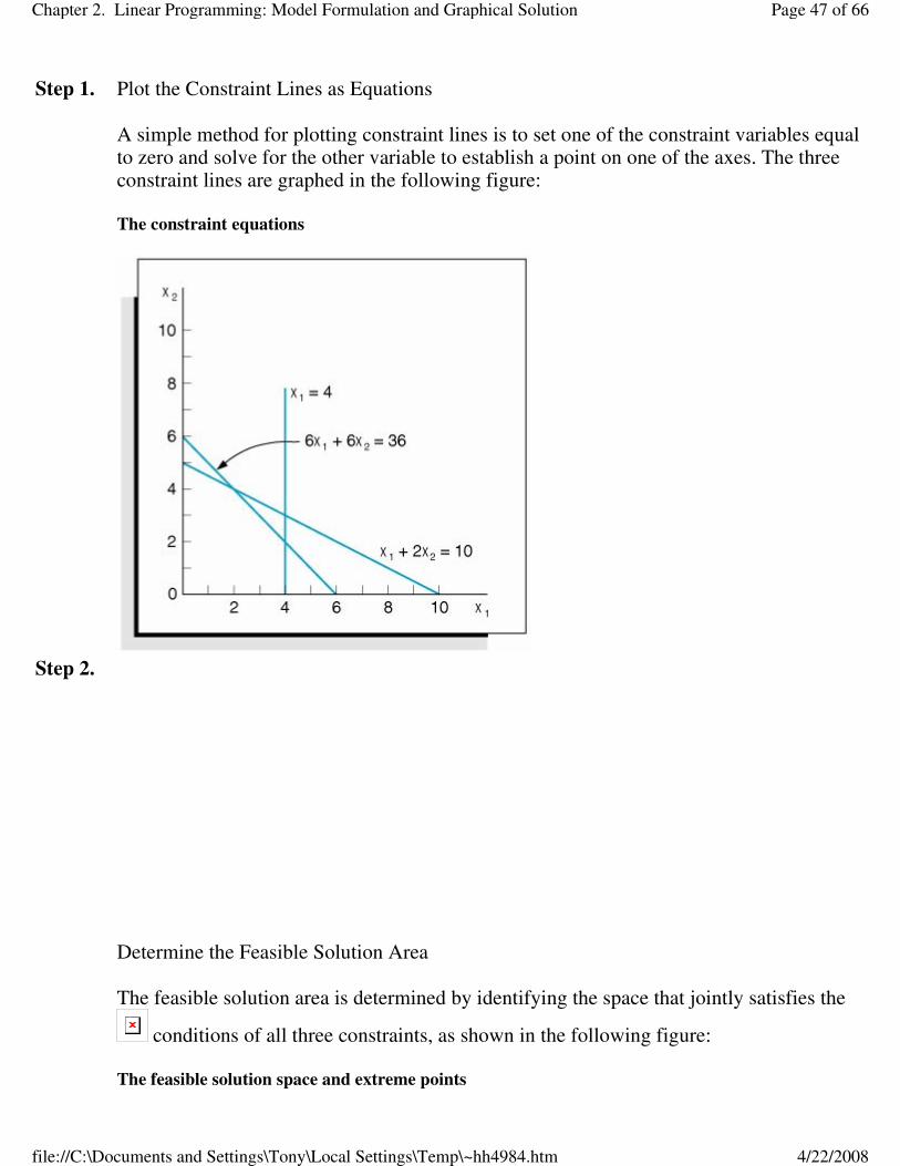
Step 1. Plot the Constraint Lines as Equations A simple method for plotting constraint lines is to set one of the constraint variables equal to zero and solve for the other variable to establish a point on one of the axes. The three constraint lines are graphed in the following figure: The constraint equations
Step 2.
Determine the Feasible Solution Area The feasible solution area is determined by identifying the space that jointly satisfies the
conditions of all three constraints, as shown in the following figure: The feasible solution space and extreme points
Page 47 of 66Chapter 2. Linear Programming: Model Formulation and Graphical Solution
4/22/2008file://C:\Documents and Settings\Tony\Local Settings\Temp\~hh4984.htm

Step 3. Determine the Solution Points The solution at point A can be determined by noting that the constraint line intersects the x
2 axis at 5; thus, x
2 = 5, x
1 = 0, and Z = 25. The solution at point D on the other axis can
be determined similarly; the constraint intersects the axis at x1 = 4, x
2 = 0, and Z = 16.
[Page 60] The values at points B and C must be found by solving simultaneous equations. Note that point B is formed by the intersection of the lines x
1 + 2x
2 = 10 and 6x
1 + 6x
2 = 36. First,
convert both of these equations to functions of x1:
and
Now set the equations equal and solve for x2:
Page 48 of 66Chapter 2. Linear Programming: Model Formulation and Graphical Solution
4/22/2008file://C:\Documents and Settings\Tony\Local Settings\Temp\~hh4984.htm

Substituting x2 = 4 into either of the two equations gives a value for x
1:
x
1 = 6 x
2
x
1 = 6 (4)
x
1 = 2
Thus, at point B, x
1 = 2, x
2 = 4, and Z = 28.
At point C, x
1 = 4. Substituting x
1 = 4 into the equation x
1 = 6 x
2 gives a value for x
2:
4 = 6 x
2
x
2 = 2
Thus, x
1 = 4, x
2 = 2, and Z = 26.
Step 4.
Determine the Optimal Solution The optimal solution is at point B, where x
1 = 2, x
2 = 4, and Z = 28. The optimal solution
and solutions at the other extreme points are summarized in the following figure: Optimal solution point
Page 49 of 66Chapter 2. Linear Programming: Model Formulation and Graphical Solution
4/22/2008file://C:\Documents and Settings\Tony\Local Settings\Temp\~hh4984.htm

[Page 61]
Problems
1. In Problem 28 in Chapter 1, when Marie McCoy wakes up Saturday morning, she remembers that she promised the PTA she would make some cakes and/or homemade bread for its bake sale that afternoon. However, she does not have time to go to the store to get ingredients, and she has only a short time to bake things in her oven. Because cakes and breads require different baking temperatures, she cannot bake them simultaneously, and she has only 3 hours available to bake. A cake requires 3 cups of flour, and a loaf of bread requires 8 cups; Marie has 20 cups of flour. A cake requires 45 minutes to bake, and a loaf of bread requires 30 minutes. The PTA will sell a cake for $10 and a loaf of bread for $6. Marie wants to decide how many cakes and loaves of bread she should make.
a. Formulate a linear programming model for this problem.
b. Solve this model by using graphical analysis.
2. A company produces two products that are processed on two assembly lines. Assembly line 1 has 100 available hours, and assembly line 2 has 42 available hours. Each product requires 10 hours of processing time on line 1, while on line 2 product 1 requires 7 hours and product 2 requires 3 hours. The profit for product 1 is $6 per unit, and the profit for product 2 is $4 per unit.
Page 50 of 66Chapter 2. Linear Programming: Model Formulation and Graphical Solution
4/22/2008file://C:\Documents and Settings\Tony\Local Settings\Temp\~hh4984.htm

a. Formulate a linear programming model for this problem.
b. Solve this model by using graphical analysis.
3. The Munchies Cereal Company makes a cereal from several ingredients. Two of the ingredients, oats and rice, provide vitamins A and B. The company wants to know how many ounces of oats and rice it should include in each box of cereal to meet the minimum requirements of 48 milligrams of vitamin A and 12 milligrams of vitamin B while minimizing cost. An ounce of oats contributes 8 milligrams of vitamin A and 1 milligram of vitamin B, whereas an ounce of rice contributes 6 milligrams of A and 2 milligrams of B. An ounce of oats costs $0.05, and an ounce of rice costs $0.03.
a. Formulate a linear programming model for this problem.
b. Solve this model by using graphical analysis.
4. What would be the effect on the optimal solution in Problem 3 if the cost of rice increased from $0.03 per ounce to $0.06 per ounce?
5. The Kalo Fertilizer Company makes a fertilizer using two chemicals that provide nitrogen, phosphate, and potassium. A pound of ingredient 1 contributes 10 ounces of nitrogen and 6 ounces of phosphate, while a pound of ingredient 2 contributes 2 ounces of nitrogen, 6 ounces of phosphate, and 1 ounce of potassium. Ingredient 1 costs $3 per pound, and ingredient 2 costs $5 per pound. The company wants to know how many pounds of each chemical ingredient to put into a bag of fertilizer to meet the minimum requirements of 20 ounces of nitrogen, 36 ounces of phosphate, and 2 ounces of potassium while minimizing cost.
a. Formulate a linear programming model for this problem.
b. Solve this model by using graphical analysis.
6. The Pinewood Furniture Company produces chairs and tables from two resourceslabor and wood. The company has 80 hours of labor and 36 pounds of wood available each day. Demand for chairs is limited to 6 per day. Each chair requires 8 hours of labor and 2 pounds of wood, whereas a table requires 10 hours of labor and 6 pounds of wood. The profit derived from each chair is $400 and from each table, $100. The company wants to determine the number of chairs and tables to produce each day in order to maximize profit.
a. Formulate a linear programming model for this problem.
b. Solve this model by using graphical analysis.
Page 51 of 66Chapter 2. Linear Programming: Model Formulation and Graphical Solution
4/22/2008file://C:\Documents and Settings\Tony\Local Settings\Temp\~hh4984.htm

[Page 62]
7. In Problem 6, how much labor and wood will be unused if the optimal numbers of chairs and tables are produced?
8. In Problem 6, explain the effect on the optimal solution of changing the profit on a table from $100 to $500.
9. The Crumb and Custard Bakery makes coffee cakes and Danish pastries in large pans. The main ingredients are flour and sugar. There are 25 pounds of flour and 16 pounds of sugar available, and the demand for coffee cakes is 5. Five pounds of flour and 2 pounds of sugar are required to make a pan of coffee cakes, and 5 pounds of flour and 4 pounds of sugar are required to make a pan of Danish. A pan of coffee cakes has a profit of $1, and a pan of Danish has a profit of $5. Determine the number of pans of cakes and Danish to produce each day so that profit will be maximized.
a. Formulate a linear programming model for this problem.
b. Solve this model by using graphical analysis.
10. In Problem 9, how much flour and sugar will be left unused if the optimal numbers of cakes and Danish are baked?
11. Solve the following linear programming model graphically:
12. The Elixer Drug Company produces a drug from two ingredients. Each ingredient contains the same three antibiotics, in different proportions. One gram of ingredient 1 contributes 3 units, and 1 gram of ingredient 2 contributes 1 unit of antibiotic 1; the drug requires 6 units. At least 4 units of antibiotic 2 are required, and the ingredients each contribute 1 unit per gram. At least 12 units of antibiotic 3 are required; a gram of ingredient 1 contributes 2 units, and a gram of ingredient 2 contributes 6 units. The cost for a gram of ingredient 1 is $80, and the cost for a gram of ingredient 2 is $50. The company wants to formulate a linear programming model to determine the number of grams of each ingredient that must go into the drug in order to meet the antibiotic requirements at the minimum cost.
Page 52 of 66Chapter 2. Linear Programming: Model Formulation and Graphical Solution
4/22/2008file://C:\Documents and Settings\Tony\Local Settings\Temp\~hh4984.htm

a. Formulate a linear programming model for this problem.
b. Solve this model by using graphical analysis.
13. A jewelry store makes necklaces and bracelets from gold and platinum. The store has 18 ounces of gold and 20 ounces of platinum. Each necklace requires 3 ounces of gold and 2 ounces of platinum, whereas each bracelet requires 2 ounces of gold and 4 ounces of platinum. The demand for bracelets is no more than four. A necklace earns $300 in profit and a bracelet, $400. The store wants to determine the number of necklaces and bracelets to make in order to maximize profit.
a. Formulate a linear programming model for this problem.
b. Solve this model by using graphical analysis.
14. In Problem 13, explain the effect on the optimal solution of increasing the profit on a bracelet from $400 to $600. What will be the effect of changing the platinum requirement for a necklace from 2 ounces to 3 ounces?
[Page 63]
15. In Problem 13:
a. The maximum demand for bracelets is four. If the store produces the optimal number of bracelets and necklaces, will the maximum demand for bracelets be met? If not, by how much will it be missed?
b. What profit for a necklace would result in no bracelets being produced, and what would be the optimal solution for this profit?
16. A clothier makes coats and slacks. The two resources required are wool cloth and labor. The clothier has 150 square yards of wool and 200 hours of labor available. Each coat requires 3 square yards of wool and 10 hours of labor, whereas each pair of slacks requires 5 square yards of wool and 4 hours of labor. The profit for a coat is $50, and the profit for slacks is $40. The clothier wants to determine the number of coats and pairs of slacks to make so that profit will be maximized.
a. Formulate a linear programming model for this problem.
b. Solve this model by using graphical analysis.
17. In Problem 16, what would be the effect on the optimal solution if the available labor were increased from 200 to 240 hours?
Page 53 of 66Chapter 2. Linear Programming: Model Formulation and Graphical Solution
4/22/2008file://C:\Documents and Settings\Tony\Local Settings\Temp\~hh4984.htm
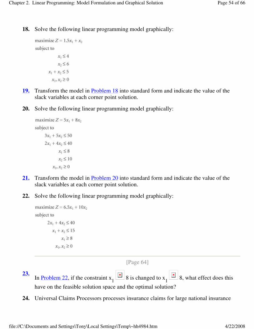
18. Solve the following linear programming model graphically:
19. Transform the model in Problem 18 into standard form and indicate the value of the slack variables at each corner point solution.
20. Solve the following linear programming model graphically:
21. Transform the model in Problem 20 into standard form and indicate the value of the slack variables at each corner point solution.
22. Solve the following linear programming model graphically:
[Page 64]
23.In Problem 22, if the constraint x
1 8 is changed to x
1 8, what effect does this
have on the feasible solution space and the optimal solution?
24. Universal Claims Processors processes insurance claims for large national insurance
Page 54 of 66Chapter 2. Linear Programming: Model Formulation and Graphical Solution
4/22/2008file://C:\Documents and Settings\Tony\Local Settings\Temp\~hh4984.htm

companies. Most claim processing is done by a large pool of computer operators, some of whom are permanent and some of whom are temporary. A permanent operator can process 16 claims per day, whereas a temporary operator can process 12 per day, and on average the company processes at least 450 claims each day. The company has 40 computer workstations. A permanent operator generates about 0.5 claims with errors each day, whereas a temporary operator averages about 1.4 defective claims per day. The company wants to limit claims with errors to 25 per day. A permanent operator is paid $64 per day, and a temporary operator is paid $42 per day. The company wants to determine the number of permanent and temporary operators to hire in order to minimize costs.
a. Formulate a linear programming model for this problem.
b. Solve this model by using graphical analysis.
25. In Problem 24, explain the effect on the optimal solution of changing the daily pay for a permanent claims processor from $64 to $54. Explain the effect of changing the daily pay for a temporary claims processor from $42 to $36.
26. In Problem 24, what would be the effect on the optimal solution if Universal Claims Processors decided not to try to limit the number of defective claims each day?
27. In Problem 24, explain the effect on the optimal solution if the minimum number of claims the firm processes each day increased from 450 to at least 650.
28. Solve the following linear programming model graphically:
29. Solve the following linear programming model graphically:
Page 55 of 66Chapter 2. Linear Programming: Model Formulation and Graphical Solution
4/22/2008file://C:\Documents and Settings\Tony\Local Settings\Temp\~hh4984.htm

30.In Problem 29, what would be the effect on the solution if the constraint x
2 7 were
changed to x2 7?
31. Solve the following linear programming model graphically:
[Page 65]
32. Solve the following linear programming model graphically:
33. Solve the following linear programming model graphically:
Page 56 of 66Chapter 2. Linear Programming: Model Formulation and Graphical Solution
4/22/2008file://C:\Documents and Settings\Tony\Local Settings\Temp\~hh4984.htm

34. Gillian's Restaurant has an ice-cream counter where it sells two main products, ice cream and frozen yogurt, each in a variety of flavors. The restaurant makes one order for ice cream and yogurt each week, and the store has enough freezer space for 115 gallons total of both products. A gallon of frozen yogurt costs $0.75 and a gallon of ice cream costs $0.93, and the restaurant budgets $90 each week for these products. The manager estimates that each week the restaurant sells at least twice as much ice cream as frozen yogurt. Profit per gallon of ice cream is $4.15, and profit per gallon of yogurt is $3.60.
a. Formulate a linear programming model for this problem.
b. Solve this model by using graphical analysis.
35. In Problem 34, how much additional profit would the restaurant realize each week if it increased its freezer capacity to accommodate 20 extra gallons total of ice cream and yogurt?
36. Copperfield Mining Company owns two mines, each of which produces three grades of orehigh, medium, and low. The company has a contract to supply a smelting company with at least 12 tons of high-grade ore, 8 tons of medium-grade ore, and 24 tons of low-grade ore. Each mine produces a certain amount of each type of ore during each hour that it operates. Mine 1 produces 6 tons of high-grade ore, 2 tons of medium-grade ore, and 4 tons of low-grade ore per hour. Mine 2 produces 2, 2, and 12 tons, respectively, of high-, medium-, and low-grade ore per hour. It costs Copperfield $200 per hour to mine each ton of ore from mine 1, and it costs $160 per hour to mine each ton of ore from mine 2. The company wants to determine the number of hours it needs to operate each mine so that its contractual obligations can be met at the lowest cost.
a. Formulate a linear programming model for this problem.
b. Solve this model by using graphical analysis.
37. A canning company produces two sizes of cansregular and large. The cans are produced in 10,000-can lots. The cans are processed through a stamping operation and a coating operation. The company has 30 days available for both stamping and coating. A lot of
Page 57 of 66Chapter 2. Linear Programming: Model Formulation and Graphical Solution
4/22/2008file://C:\Documents and Settings\Tony\Local Settings\Temp\~hh4984.htm

regular-size cans requires 2 days to stamp and 4 days to coat, whereas a lot of large cans requires 4 days to stamp and 2 days to coat. A lot of regular-size cans earns $800 profit, and a lot of large-size cans earns $900 profit. In order to fulfill its obligations under a shipping contract, the company must produce at least nine lots. The company wants to determine the number of lots to produce of each size can (x
1 and x
2) in order to
maximize profit.
[Page 66]
a. Formulate a linear programming model for this problem.
b. Solve this model by using graphical analysis.
38. A manufacturing firm produces two products. Each product must undergo an assembly process and a finishing process. It is then transferred to the warehouse, which has space for only a limited number of items. The firm has 80 hours available for assembly and 112 hours for finishing, and it can store a maximum of 10 units in the warehouse. Each unit of product 1 has a profit of $30 and requires 4 hours to assemble and 14 hours to finish. Each unit of product 2 has a profit of $70 and requires 10 hours to assemble and 8 hours to finish. The firm wants to determine the quantity of each product to produce in order to maximize profit.
a. Formulate a linear programming model for this problem.
b. Solve this model by using graphical analysis.
39. Assume that the objective function in Problem 38 has been changed from Z = 30x1 +
70x2 to Z = 90x
1 + 70x
2. Determine the slope of each objective function and discuss
what effect these slopes have on the optimal solution.
40. The Valley Wine Company produces two kinds of wineValley Nectar and Valley Red. The wines are produced from 64 tons of grapes the company has acquired this season. A 1,000-gallon batch of Nectar requires 4 tons of grapes, and a batch of Red requires 8 tons. However, production is limited by the availability of only 50 cubic yards of storage space for aging and 120 hours of processing time. A batch of each type of wine
requires 5 yd.3 of storage space. The processing time for a batch of Nectar is 15 hours,
and the processing time for a batch of Red is 8 hours. Demand for each type of wine is limited to seven batches. The profit for a batch of Nectar is $9,000, and the profit for a batch of Red is $12,000. The company wants to determine the number of 1,000-gallon batches of Nectar (x
1) and Red (x
2) to produce in order to maximize profit.
Page 58 of 66Chapter 2. Linear Programming: Model Formulation and Graphical Solution
4/22/2008file://C:\Documents and Settings\Tony\Local Settings\Temp\~hh4984.htm

a. Formulate a linear programming model for this problem.
b. Solve this model by using graphical analysis.
41. In Problem 40:
1. How much processing time will be left unused at the optimal solution?
2. What would be the effect on the optimal solution of increasing the available
storage space from 50 to 60 yd.3?
42. Kroeger supermarket sells its own brand of canned peas as well as several national brands. The store makes a profit of $0.28 per can for its own peas and a profit of $0.19 for any of the national brands. The store has 6 square feet of shelf space available for canned peas, and each can of peas takes up 9 square inches of that space. Point-of-sale records show that each week the store never sells more than one-half as many cans of its own brand as it does of the national brands. The store wants to know how many cans of its own brand of peas and how many cans of the national brands to stock each week on the allocated shelf space in order to maximize profit.
a. Formulate a linear programming model for this problem.
b. Solve this model by using graphical analysis.
43. In Problem 42, if Kroeger discounts the price of its own brand of peas, the store will sell at least 1.5 times as much of the national brands as its own brand, but its profit margin on its own brand will be reduced to $0.23 per can. What effect would the discount have on the optimal solution?
44. Shirtstop makes T-shirts with logos and sells them in its chain of retail stores. It contracts with two different plantsone in Puerto Rico and one in The Bahamas. The shirts from the plant in Puerto Rico cost $0.46 a piece, and 9% of them are defective and can't be sold. The shirts from The Bahamas cost only $0.35 each, but they have an 18% defective rate. Shirtstop needs 3,500 shirts. To retain its relationship with the two plants, it wants to order at least 1,000 shirts from each. It would also like at least 88% of the shirts it receives to be salable.
[Page 67]
a. Formulate a linear programming model for this problem.
b. Solve this model by using graphical analysis.
Page 59 of 66Chapter 2. Linear Programming: Model Formulation and Graphical Solution
4/22/2008file://C:\Documents and Settings\Tony\Local Settings\Temp\~hh4984.htm

45. In Problem 44:
a. Suppose Shirtstop decided it wanted to minimize the defective shirts while keeping costs below $2,000. Reformulate the problem with these changes and solve graphically.
b. How many fewer defective items were achieved with the model in (a) than with the model in Problem 44?
46. Angela and Bob Ray keep a large garden in which they grow cabbage, tomatoes, and onions to make two kinds of relishchow-chow and tomato. The chow-chow is made primarily of cabbage, whereas the tomato relish has more tomatoes than chow-chow. Both relishes include onions, and negligible amounts of bell peppers and spices. A jar of chow-chow contains 8 ounces of cabbage, 3 ounces of tomatoes, and 3 ounces of onions, whereas a jar of tomato relish contains 6 ounces of tomatoes, 6 ounces of cabbage, and 2 ounces of onions. The Rays grow 120 pounds of cabbage, 90 pounds of tomatoes, and 45 pounds of onions each summer. The Rays can produce no more than 24 dozen jars of relish. They make $2.25 in profit from a jar of chow-chow and $1.95 in profit from a jar of tomato relish. The Rays want to know how many jars of each kind of relish to produce to generate the most profit.
a. Formulate a linear programming model for this problem.
b. Solve this model graphically.
47. In Problem 46, the Rays have checked their sales records for the past five years and have found that they sell at least 50% more chow-chow than tomato relish. How will this additional information affect their model and solution?
48. A California grower has a 50-acre farm on which to plant strawberries and tomatoes. The grower has available 300 hours of labor per week and 800 tons of fertilizer, and he has contracted for shipping space for a maximum of 26 acres' worth of strawberries and 37 acres' worth of tomatoes. An acre of strawberries requires 10 hours of labor and 8 tons of fertilizer, whereas an acre of tomatoes requires 3 hours of labor and 20 tons of fertilizer. The profit from an acre of strawberries is $400, and the profit from an acre of tomatoes is $300. The farmer wants to know the number of acres of strawberries and tomatoes to plant to maximize profit.
a. Formulate a linear programming model for this problem.
b. Solve this model by using graphical analysis.
49. In Problem 48, if the amount of fertilizer required for each acre of strawberries were determined to be 20 tons instead of 8 tons, what would be the effect on the optimal
Page 60 of 66Chapter 2. Linear Programming: Model Formulation and Graphical Solution
4/22/2008file://C:\Documents and Settings\Tony\Local Settings\Temp\~hh4984.htm

solution?
50. The admissions office at Tech wants to determine how many in-state and how many out-of-state students to accept for next fall's entering freshman class. Tuition for an in-state student is $7,600 per year, whereas out-of-state tuition is $22,500 per year. A total of 12,800 in-state and 8,100 out-of-state freshmen have applied for next fall, and Tech does not want to accept more than 3,500 students. However, because Tech is a state institution, the state mandates that it can accept no more than 40% out-of-state students. From past experience the admissions office knows that 12% of in-state students and 24% of out-of-state students will drop out during their first year. Tech wants to maximize total tuition while limiting the total attrition to 600 first-year students.
1. Formulate a linear programming model for this problem.
2. Solve this model by using graphical analysis.
[Page 68]
51. Janet Lopez is establishing an investment portfolio that will include stock and bond funds. She has $720,000 to invest, and she does not want the portfolio to include more than 65% stocks. The average annual return for the stock fund she plans to invest in is 18%, whereas the average annual return for the bond fund is 6%. She further estimates that the most she could lose in the next year in the stock fund is 22%, whereas the most she could lose in the bond fund is 5%. To reduce her risk, she wants to limit her potential maximum losses to $100,000.
a. Formulate a linear programming model for this problem.
b. Solve this model by using graphical analysis.
52. Professor Smith teaches two sections of business statistics, which combined will result in 120 final exams to be graded. Professor Smith has two graduate assistants. Brad and Sarah, who will grade the final exams. There is a 3-day period between the time the exam is administered and when final grades must be posted. During this period Brad has 12 hours available and Sarah has 10 hours available to grade the exams. It takes Brad an average of 7.2 minutes to grade an exam, and it takes Sarah 12 minutes to grade an exam; however, Brad's exams will have errors that will require Professor Smith to ultimately regrade 10% of the exams, while only 6% of Sarah's exams will require regrading. Professor Smith wants to know how many exams to assign to each graduate assistant to grade in order to minimize the number of exams to regrade.
a. Formulate a linear programming model for this problem.
Page 61 of 66Chapter 2. Linear Programming: Model Formulation and Graphical Solution
4/22/2008file://C:\Documents and Settings\Tony\Local Settings\Temp\~hh4984.htm

b. Solve this model by using graphical analysis.
53. In Problem 52, if Professor Smith could hire Brad or Sarah to work 1 additional hour, which should she choose? What would be the effect of hiring the selected graduate assistant for 1 additional hour?
54. Starbright Coffee Shop at the Galleria Mall serves two coffee blends it brews on a daily basis, Pomona and Coastal. Each is a blend of three high-quality coffees from Colombia, Kenya, and Indonesia. The coffee shop has 10 pounds of each of these coffees available each day. Each pound of coffee will produce sixteen 16-ounce cups of coffee. The shop has enough brewing capacity to brew 30 gallons of these two coffee blends each day. Pomona is a blend of 20% Colombian, 35% Kenyan, and 45% Indonesian, while Coastal is a blend of 60% Colombian, 10% Kenyan, and 30% Indonesian. The shop sells 1.5 times more Pomona than Coastal each day. Pomona sells for $2.05 per cup, and Coastal sells for $1.85 per cup. The manager wants to know how many cups of each blend to sell each day in order to maximize sales.
a. Formulate a linear programming model for this problem.
b. Solve this model by using graphical analysis.
55. In Problem 54:
a. If Starbright Coffee Shop could get 1 more pound of coffee, which one should it be? What would be the effect on sales of getting 1 more pound of this coffee? Would it benefit the shop to increase its brewing capacity from 30 gallons to 40 gallons?
b. If the shop spent $20 per day on advertising that would increase the relative demand for Pomona to twice that of Coastal, should it be done?
56. Solve the following linear programming model graphically and explain the solution result:
[Page 69]
Page 62 of 66Chapter 2. Linear Programming: Model Formulation and Graphical Solution
4/22/2008file://C:\Documents and Settings\Tony\Local Settings\Temp\~hh4984.htm

57. Solve the following linear programming model graphically and explain the solution result:
58. Solve the following linear programming model graphically and explain the solution result:
[Page 69 (continued)]
Case Problem
METROPOLITAN POLICE PATROL
The Metropolitan Police Department had recently been criticized in the local media for not responding to police calls in the downtown area rapidly enough. In several recent cases, alarms had sounded for break-ins, but by the time the police car arrived, the perpetrators had left, and in one instance a store owner had been shot. Sergeant Joe Davis had been assigned by the chief as head of a task force to find a way to determine the optimal patrol area (dimensions) for their cars that would minimize the average time it took to respond to a call in the downtown area.
Sergeant Davis solicited help from Angela Maris, an analyst in the operations area for the police department. Together they began to work through the problem.
Joe noted to Angela that normal patrol sectors are laid out in rectangles, with each rectangle including a number of city blocks. For illustrative purposes he defined the dimensions of the sector as x in the horizontal direction and as y in the vertical direction. He explained to Angela that cars traveled in straight lines either horizontally or vertically and turned at right angles. Travel in a
Page 63 of 66Chapter 2. Linear Programming: Model Formulation and Graphical Solution
4/22/2008file://C:\Documents and Settings\Tony\Local Settings\Temp\~hh4984.htm

horizontal direction must be accompanied by travel in a vertical direction, and the total distance traveled is the sum of the horizontal and vertical segments. He further noted that past research on police patrolling in urban areas had shown that the average distance traveled by a patrol car responding to a call in either direction was one-third of the dimensions of the sector, or x/3 and y/3. He also explained that the travel time it took to respond to a call (assuming that a car left immediately upon receiving the call) is simply the average distance traveled divided by the average travel speed.
Angela told Joe that now that she understood how average travel time to a call was determined, she could see that it was closely related to the size of the patrol area. She asked Joe if there were any restrictions on the size of the area sectors that cars patrolled. He responded that for their city, the department believed that the perimeter of a patrol sector should not be less than 5 miles or exceed 12 miles. He noted several policy issues and staffing constraints that required these specifications. Angela wanted to know if any additional restrictions existed, and Joe indicated that the distance in the vertical direction must be at least 50% more than the horizontal distance for the sector. He explained that laying out sectors in that manner meant that the patrol areas would have a greater tendency to overlap different residential, income, and retail areas than if they ran the other way. He said that these areas were layered from north to south in the city. So if a sector area were laid out east to west, all of it would tend to be in one demographic layer.
Angela indicated that she had almost enough information to develop a model, except that she also needed to know the average travel speed the patrol cars could travel. Joe told her that cars moving vertically traveled an average of 15 miles per hour, whereas cars traveled horizontally an average of 20 miles per hour. He said that the difference was due to different traffic flows.
Develop a linear programming model for this problem and solve it by using the graphical method.
[Page 70]
Case Problem
"THE POSSIBILITY" RESTAURANT
Angela Fox and Zooey Caulfield were food and nutrition majors at State University, as well as close friends and roommates. Upon graduation Angela and Zooey decided to open a French restaurant in Draperton, the small town where the university was located. There were no other French restaurants in Draperton, and the possibility of doing something new and somewhat risky intrigued the two friends. They purchased an old Victorian home just off Main Street for their new restaurant, which they named "The Possibility."
Angela and Zooey knew in advance that at least initially they could not offer a full, varied menu of dishes. They had no idea what their local customers' tastes in French cuisine would be, so they
Page 64 of 66Chapter 2. Linear Programming: Model Formulation and Graphical Solution
4/22/2008file://C:\Documents and Settings\Tony\Local Settings\Temp\~hh4984.htm

decided to serve only two full-course meals each night, one with beef and the other with fish. Their chef, Pierre, was confident he could make each dish so exciting and unique that two meals would be sufficient, at least until they could assess which menu items were most popular. Pierre indicated that with each meal he could experiment with different appetizers, soups, salads, vegetable dishes, and desserts until they were able to identify a full selection of menu items.
The next problem for Angela and Zooey was to determine how many meals to prepare for each night so they could shop for ingredients and set up the work schedule. They could not afford too much waste. They estimated that they would sell a maximum of 60 meals each night. Each fish dinner, including all accompaniments, requires 15 minutes to prepare, and each beef dinner takes twice as long. There is a total of 20 hours of kitchen staff labor available each day. Angela and Zooey believe that because of the health consciousness of their potential clientele, they will sell at least three fish dinners for every two beef dinners. However, they also believe that at least 10% of their customers will order beef dinners. The profit from each fish dinner will be approximately $12, and the profit from a beef dinner will be about $16.
Formulate a linear programming model for Angela and Zooey that will help them estimate the number of meals they should prepare each night and solve this model graphically.
If Angela and Zooey increased the menu price on the fish dinner so that the profit for both dinners was the same, what effect would that have on their solution? Suppose Angela and Zooey reconsidered the demand for beef dinners and decided that at least 20% of their customers would purchase beef dinners. What effect would this have on their meal preparation plan?
[Page 70 (continued)]
Case Problem
ANNABELLE INVESTS IN THE MARKET
Annabelle Sizemore has cashed in some treasury bonds and a life insurance policy that her parents had accumulated over the years for her. She has also saved some money in certificates of deposit and savings bonds during the 10 years since she graduated from college. As a result, she has $120,000 available to invest. Given the recent rise in the stock market, she feels that she should invest all of this amount there. She has researched the market and has decided that she wants to invest in an index fund tied to S&P stocks and in an Internet stock fund. However, she is very concerned about the volatility of Internet stocks. Therefore, she wants to balance her risk to some degree.
She has decided to select an index fund from Shield Securities and an Internet stock fund from Madison Funds, Inc. She has also decided that the proportion of the dollar amount she invests in the index fund relative to the Internet fund should be at least one-third but that she should not invest
Page 65 of 66Chapter 2. Linear Programming: Model Formulation and Graphical Solution
4/22/2008file://C:\Documents and Settings\Tony\Local Settings\Temp\~hh4984.htm
more than twice the amount in the Internet fund that she invests in the index fund. The price per share of the index fund is $175, whereas the price per share of the Internet fund is $208. The average annual return during the last 3 years for the index fund has been 17%, and for the Internet stock fund it has been 28%. She anticipates that both mutual funds will realize the same average returns for the coming year that they have in the recent past; however, at the end of the year she is likely to reevaluate her investment strategy anyway. Thus, she wants to develop an investment strategy that will maximize her return for the coming year.
Formulate a linear programming model for Annabelle that will indicate how much money she should invest in each fund and solve this model by using the graphical method.
Suppose Annabelle decides to change her risk-balancing formula by eliminating the restriction that the proportion of the amount she invests in the index fund to the amount that she invests in the Internet fund must be at least one-third. What will the effect be on her solution? Suppose instead that she eliminates the restriction that the proportion of money she invests in the Internet fund relative to the stock fund not exceed a ratio of 2 to 1. How will this affect her solution?
If Annabelle can get $1 more to invest, how will that affect her solution? $2 more? $3 more? What can you say about her return on her investment strategy, given these successive changes?
Page 66 of 66Chapter 2. Linear Programming: Model Formulation and Graphical Solution
4/22/2008file://C:\Documents and Settings\Tony\Local Settings\Temp\~hh4984.htm