arX

iv:1

210.

7164

v3 [

q-bi

o.C

B]

5 J

un 2

013

Vascular networks due to dynamically arrested crystalline

ordering of elongated cells

Margriet M. Palm1, 2, ∗ and Roeland M. H. Merks1, 2, 3, †

1Centrum Wiskunde & Informatica, Amsterdam, The Netherlands

2Netherlands Consortium for Systems Biology - Netherlands

Institute for Systems Biology, Amsterdam, The Netherlands

3Mathematical Institute, Leiden University, Leiden, The Netherlands

(Dated: September 16, 2018)

Abstract

Recent experimental and theoretical studies suggest that crystallization and glass-like solidifica-

tion are useful analogies for understanding cell ordering in confluent biological tissues. It remains

unexplored how cellular ordering contributes to pattern formation during morphogenesis. With

a computational model we show that a system of elongated, cohering biological cells can get dy-

namically arrested in a network pattern. Our model provides a new explanation for the formation

of cellular networks in culture systems that exclude intercellular interaction via chemotaxis or

mechanical traction.

PACS numbers: 87.17.Jj,87.18.Hf,87.17.Pq

∗Electronic address: M.M.Palm@cwi.nl†Electronic address: merks@cwi.nl

1

I. INTRODUCTION

By aligning locally with one another, cells of elongated shape form ordered, crystalline

configurations in cell cultures of, e.g. fibroblasts [1, 2], mesenchymal stem cells [2], and

endothelial cells [3]. Initially the cells form small clusters of aligned cells; the clusters then

grow and the range over which cells align increases with time [2, 4]. To study the emergence

of such crystalline cellular ordering, it is useful to make an analogy with liquid crystals

[2]. For example, a “cellular temperature” can be defined to describe the cell-type specific

persistence (low cellular temperature) or randomness (high cellular temperature) of cell

motility, where cells of high cellular temperature (e.g., fibroblasts) are less likely to form

crystalline configurations than cells of low temperature (e.g., mesenchymal stem cells) [2]. It

was similarly proposed that collective cell motion in crowded cell sheets can be understood as

system approaching a glass transition [5, 6]. Although these studies provide useful insights

into the ordering of cells in confluent cell layers, it remains unexplored how crystallization

and glass-like dynamics contribute to the formation of more complex shapes and patterns

during biological morphogenesis.

Cells’ organizing into network-like structures, as it occurs for example during blood vessel

development, is a suitable system to study how cellular ordering participates in pattern

formation. In cell cultures after stimulation by growth factors (VEGFs, FGFs), endothelial

cells elongate and form vascular-like network structures [7–9]. The mechanisms that drive

the aggregation of endothelial cells and their subsequent organization into network is a

subject of debate. Most models assume an attractive force between cells, either due to

chemotaxis [10–18] or due to mechanical traction via the extracellular matrix [19–24]. In

vitro experiments show that astroglia-related rat C6 cells and muscle-related C212 cells can

form network-like structures on a rigid culture substrate [25], which excludes formation of

mechanical or chemical attraction between cells. Therefore a second class of explanations

proposed that cells form networks by adhering better to locally elongated configurations of

cells [25] or elongated cells [26]. Here we show that, in absence of mechanical or chemical

fields such mechanisms are unnecessary: elongated cells organize into network structures

if they move and rotate randomly, and adhere to adjacent cells. As the cells align locally

with one another, a network pattern appears. Additional, long-range cell-cell attraction

mechanisms, e.g., chemotaxis or mechanotaxis, act to stabilize the pattern and fix its wave

2

length.

Long

(a)

Round

Chemotaxis

(b) (c)

Long

Chemotaxis

FIG. 1: Effect of chemotaxis and cell shape on pattern formation. A round, chemotacting,

and adhesive cells (10,000 MCS), B elongated, chemotacting and adhesive cells (10,000

MCS), and C elongated, non-chemotacting and adhesive cells (250,000 MCS). In all panels

700 cells are seeded on the center 500x500 pixels of an 800x800 lattice.

II. MODEL DESCRIPTION

To model the collective movement of elongated cells, we use the cellular Potts method

(CPM), aka the Glazier-Graner-Hogeweg model [27, 28], a lattice-based, Monte-Carlo model

that has been used to model developmental mechanisms including somitogenesis [29, 30],

convergent extension [31] and fruit fly retinal patterning [32]. The CPM represents cells as

connected patches of lattice sites with identical spin σ ∈ N; lattice sites with spin σ = 0

represent the extracellular matrix (ECM). To simulate stochastic cell motility, the CPM

iteratively displaces cell-cell and cell-ECM boundaries by attempting to copy the spin of

a randomly selected site into a randomly selected adjacent lattice site ~x, monitoring the

resulting change ∆H of a Hamiltonian,

H =∑

(~x,~x′)

J(σ(~x), σ(~x′)) (1− δ(σ(~x), σ(~x′)))

+∑

σ

λA (a(σ)−A)2 +∑

σ

λL (l(σ)− L)2 . (1)

3

A copy attempt will always be accepted if ∆H ≤ 0, if ∆H > 0 a copy attempt is accepted

with the Boltzmann probability P (∆H) = exp(−∆H/µ(σ)), with µ(σ) a “cellular temper-

ature” to simulate cell-autonomous random motility. For simplicity, we here assume that

all cells have identical temperature. The time unit is a Monte Carlo step (MCS), which

corresponds with as many copy attempts as there are lattice sites.

The first term of Eq. 1 defines an adhesion energy, with the Kronecker delta returning a

value of 1 for site pairs at cell-cell and cell-ECM interfaces, or zero otherwise. In the model

two contact energies are defined: Jcell,cell for σ > 0 at both lattice sites, and Jcell,ECM for

σ = 0 at one lattice site. The second and third term are shape constraints that penalize

deviations from a target shape, with A and L a target area and length, and a(σ) and l(σ)

the current area and length of the cell; λA and λL are shape parameters. We efficiently

estimate l(σ) by keeping track of a cellular inertia tensor as previously described [14].

In a subset of simulations, we further assume that cells secrete a diffusing chemoattractant

c, which we describe with a partial differential equation:

∂c(~x, t)

∂t= D∇2c(~x, t) + s(1− δ(σ(~x), 0))− ǫ δ(σ(~x), 0)), (2)

with diffusion constant D, secretion rate s and decay rate ǫ. After each MCS, a forward

Euler method solves Eq. 2 for 15 steps with ∆t = 2 s with zero boundary conditions. To

model the cells’ chemotaxis up concentration gradients of the chemoattractant, during each

copy attempt from ~x to ~x′ we increase ∆H with a ∆Hchemotaxis = λc (c(~x)− c(~x′)), with λc

a chemotactic strength [33]. One lattice unit (l.u.) corresponds with 2 µm. We use the

following parameter settings, unless specified otherwise: µ = 1; Jcell,cell = .5; Jcell,ECM = .35;

λA = 1; λL = .1; λc = 10; A = 100 l.u.2; L = 60 l.u.; D = 10−13 m2s−1; ǫ = 1.8 · 10−4 s−1;

s = 1.8 ·10−4 s−1. Unless stated otherwise, a simulation is initialized with 175 cells randomly

distributed on a 220x220 area at the center of a 400x400 lattice.

III. RESULTS

As Fig. 1 shows, and in agreement with previous reports [14], if we allow for chemotaxis,

rounded cells accumulate into rounded clusters (Fig. 1A) and elongated cells aggregate into

networks (Fig. 1B). Interestingly, however, chemotaxis is not required for network formation:

cell-cell adhesion between elongated cells suffices for forming networks (Fig. 1B). Movies

4

FIG. 2: Crystalline cell ordering during network formation. A-B θ(~x, r) with r = 3 for a

simulation with chemotaxis (A) and without chemotaxis (B) after 25,000 MCS. C

Temporal evolution of orientational order parameter S(r) for r = 20 (black curves), r = 40

(gray curves) and r → ∞ (light gray) without chemotaxis (solid) and with chemotaxis

(dashed). Order parameter is averaged over 10 simulation repeats (gray shadows represent

standard deviation).

corresponding with Fig. 1B and C [41] suggest that the gradual alignment of cells with

their neighbors is key to network formation and network evolution. To characterize this cell

alignment, we define θ(~x, r) as the angle between the direction of the long axis ~v(σ(~x)) of

the cell at ~x, and a local director ~n(~x, r), a weighted local average of cell orientations defined

at radius r around ~x: ~n(~x, r) = 〈~v(σ(~y))〉{~y∈Z2:|~x−~y|<r}. Figure 2A and B depict the value

of θ(~x, 3) for simulations without chemotaxis (Fig. 2A) and with chemotaxis (Fig. 2B),

with dark gray values indicating values of θ(~x, 3) → π/2. Network branches are separated

by large values of θ(~x, 3), indicating that within branches cells are aligned, whereas branch

points are “lattice defects” in which cells with different orientations meet.

Supplemental Movies S3 and S4 [42] show how the cells align gradually over time in the

5

absence and presence of chemotaxis. To characterize the temporal development of cell align-

ment in more detail, we use an orientational order parameter S(r) =⟨

cos(2θ( ~X(σ), r))⟩

σ

[34] with ~X(σ) the center of mass of cell σ. S ranges from 0 for randomly oriented cells to

1 for cells oriented in parallel.

Figure 2C shows the evolution of the global orientational order parameter limr→∞ S(r)

and of the local orientational order parameters S(20) and S(40). Both with chemotaxis

(dashed lines) and without (solid lines), S(20) grows more quickly and reaches higher order-

ing than S(40). The reason for this is that in cells of length 50−60 l.u., S(20) (covering cells

up to a radius r = 20 from the cell’s center of mass) only detects lateral alignment of cells,

whereas a radius S(40) also detects linear line-up of cells. Thus cell-cell adhesion of long

cells quickly aligns cells with the left and right neighbors, while it aligns them more slowly

with those in front and behind. This results in networks with short branches of aligned cells.

Interestingly, chemotaxis aligns cells more rapidly, both along the short and long sides of

cells, resulting in networks with much longer branches than with adhesion alone.

FIG. 3: Relation between cluster size and cell displacement. Clusters are calculated for

each morphology between 500 and 25,0000 MCS (100 simulation repeats), with an interval

of 500 MCS; see text for details. The error bars represent the standard error of the linear

fits used to estimate diffusion coefficients.

Next we analyze the mechanisms that drive the orientational ordering in the cell networks.

Visual inspection of the simulation movies suggests that single cells move and rotate much

more rapidly than locally aligned clusters of cells. A network of locally aligned cells forms

6

rapidly from initially dispersed cells. Merging of branches seems to be a much slower process,

and potentially prevents a further evolution to global nematic order. To quantify these

observations we measured the translational and rotational diffusion coefficients of cells as

a function of the size of the network branch to which it belongs. We loosely define a

network branch, or cluster of aligned cells as a connected set of at least two cells with

relative orientations < 5◦, i.e., in Fig. 2A and B dark gray values separate the clusters.

To detect clusters computationally, we first identify the connected sets for which θ(~x, 3) ≤

5◦, which are surrounded by lattice sites of σ = 0 or sites with θ(~x, 3) > 5◦. We then

eliminate connected sets of fewer than fifty lattice sites. The CPM cells sharing at least

50% of their lattice sites with one of the remaining sets form a cluster. The translational

diffusion coefficient, Dt, derives from the mean square displacement (MSD) of a set of cells:⟨

| ~X(σ, t)− ~X(σ, 0)|2⟩

σ= 4Dtt. Similarly, the rotational diffusion coefficient, Dr, derives

from the mean square rotation (MSR) of a set of cells: 〈(α(σ, t)− α(σ, 0))2〉σ = 2Drt, with

α(σ, t)−α(σ, 0) the angular displacement of a cell between time 0 and t. During a simulation,

cells may move between clusters, and clusters can merge. Therefore, to calculate Dt and

Dr of cells as a function of cluster size, for 100 simulations of 250,000 MCS we measured

trajectories of each individual cell with one data point per 500 MCS, and kept track of the

size of the cluster it was classified into at each time point. We defined cluster size bins, with

the first bin collecting all clusters consisting of two to five cells, and the next bins running

from 6 to 10, 11 to 15, etc. We split up the trajectories into chunks of 10 consecutive data

points, during which the cells stayed within clusters belonging to one bin. To calculate Dt

and Dr we performed a least square fitting on the binned MSD and MSR values for these

trajectory chunks.

The translational diffusion, Dt, increases slightly with cluster size (Fig. 3A). This may

reflect that the probability of hopping between small clusters will be larger than the proba-

bility of hopping between larger clusters, resulting in an overrepresentation of slow cells in

the small clusters. Interestingly, the rotational diffusion Dr drops with the cluster size (Fig.

3B), indicating that cells in large clusters rotate more slowly. These results suggest that the

rotation of cells in big clusters is limited, which reduces the probability that two clusters

rotate and merge into a single larger cluster. Therefore, if the size of clusters increases,

their rotation speeds drop as does the probability of cluster fusion. Thus, although further

alignment of clusters would reduce the pattern energy H (Eq. 1), the pattern evolution

7

essentially freezes.

To corroborate our hypothesis that network patterns are transient patterns that increas-

ingly slowly evolve towards nematic order, we looked for model parameters that could speed

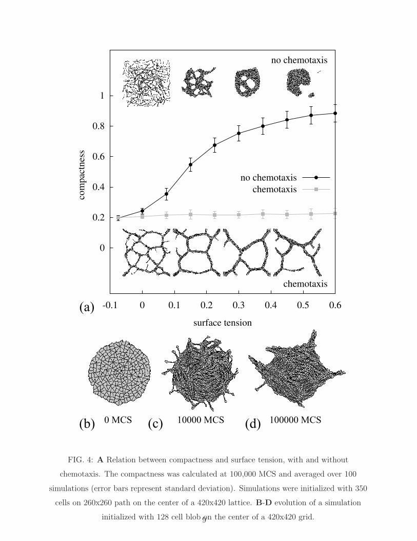
up pattern evolution. Fig. 4A shows the effect of surface tension (γcell,ECM) on the ability

of cells to form networks after 100,000 MCS, as expressed by the configuration’s compact-

ness C = Acells

Ahull, where Ahull is the area of the convex hull of the largest connected group

of cells, and Acells is the summed area of the cells inside the hull. A value of C → 1

indicates a spheroid of cells, where for networks C would tend to zero. For values of

γcell,ECM = Jcell,ECM −Jcell,cell

2> 0, the equilibrium pattern should minimize its surface area

with the ECM. Indeed at increased surface tensions the cells settle down in spheroids or

networks with only few meshes, although they initially still form network-like patterns (see

Movie S5 [43]). To confirm that also for γcell,ECM = 0.1 (i.e., the values used in Figs. 1-

3) spheroids are stable configurations, we initialized our model with a spheroid (Fig. 4B).

Although initially some cells sprout (Fig. 4C) from the spheroid due to their elongation,

they then align gradually and the cell cluster remains spherical. No network formation was

detected in simulations of 100,000 MCS (Fig. 4D), suggesting that spheroids represent the

global minimum of the Hamiltonian. Interestingly, in presence of chemotaxis networks form

for a wide range of surface tensions (inset Fig. 4A and [14]).

IV. DISCUSSION

Our analysis suggests that in the cellular Potts model elongated, adhesive cells can form

networks in a parameter regime where a spheroid pattern is the minimal energy state. The

cells initially align with nearby cells, thus forming the branches of the network. In order

for the pattern to evolve further towards the minimal-energy spheroid pattern, the locally

aligned clusters of cells must join adjacent branches, for which they must move and rotate.

Our analysis of the rotational and translational diffusion of cells in Fig. 3 shows that this

becomes more difficult for cells belonging to larger clusters. Thus the networks evolve

ever more slowly to the minimal energy state, and gets dynamically arrested in a network-

like configuration, a phenomenon reminiscent of the glass transition, as e.g. observed in

attractive colloid systems [35], collective cell migration of biological cells in vitro [5, 6], and

colloid rod suspensions [36] in which gels can form from clusters of parallel rods [37–39].

8

0

0.2

0.4

0.6

0.8

1

-0.1 0 0.1 0.2 0.3 0.4 0.5 0.6

compactness

surface tension

no chemotaxis

chemotaxis

no chemotaxis

chemotaxis

(a)

(b) (d)(c)0 MCS 100000 MCS10000 MCS

FIG. 4: A Relation between compactness and surface tension, with and without

chemotaxis. The compactness was calculated at 100,000 MCS and averaged over 100

simulations (error bars represent standard deviation). Simulations were initialized with 350

cells on 260x260 path on the center of a 420x420 lattice. B-D evolution of a simulation

initialized with 128 cell blob on the center of a 420x420 grid.9

Fig. 4A suggests that the cellular Potts simulations undergo a glass transition as the

surface tension drops: for high surface tension the system evolves towards equilibrium,

for lower surface tensions the system becomes jammed in a network-like state. Thus our

model provides a new explanation for the formation of vascular networks in absence of

chemical or mechanical, long-range, intercellular attraction [25]. Interestingly, intercellular

attraction via chemotaxis stabilizes the formation of networks in our simulations [14] and can

drive sprouting from spheroids (not shown). This suggests that networks are an equilibrium

pattern of our system in presence of intercellular attraction. Nevertheless the present analysis

of arrested dynamics provides new insight into the system with intercellular attraction:

chemotaxis reinforces local ordering over a distance proportional to the diffusion length of

the chemoattractant producing networks of a scale independent of surface tension [14].

Acknowledgments

The authors thank the IU and the Biocomplexity Institute for providing the CC3D mod-

eling environment (www.compucell3d.org) [40] and SARA for providing access to The Na-

tional Compute Cluster LISA (www.sara.nl). This work was financed by the Netherlands

Consortium for Systems Biology (NCSB) which is part of the Netherlands Genomics Ini-

tiative/Netherlands. The investigations were in part supported by the Division for Earth

and Life Sciences (ALW) with financial aid from the Netherlands Organization for Scientific

Research (NWO).

[1] T. R. Elsdale, Exp. Cell Res. 51, 439 (1968).

[2] A. Pietak and S. D. Waldman, Phys. Biol. 5, 016007 (2008).

[3] A. Szabo, R. Unnep, E. Mehes, W. O. Twal, W. S. Argraves, Y. Cao, and A. Czirok, Phys.

Biol. 7, 046007 (2010).

[4] T. Elsdale and F. Wasoff, Dev. Genes Evol. 147, 121 (1976).

[5] T. E. Angelini, E. Hannezo, X. Trepat, M. Marquez, J. J. Fredberg, and D. A. Weitz, P. Natl.

Acad. Sci. U.S.A. pp. 1–6 (2011).

[6] J. P. Garrahan, P. Natl. Acad. Sci. U.S.A. 108, 4701 (2011).

10

[7] Y. Cao, P. Linden, J. Farnebo, R. Cao, A. Eriksson, V. Kumar, J. H. Qi, L. Claesson-Welsh,

and K. Alitalo, P. Natl. Acad. Sci. U.S.A. 95, 14389 (1998).

[8] C. J. Drake, A. LaRue, N. Ferrara, and C. D. Little, Dev. Biol. 224, 178 (2000).

[9] H. Parsa, R. Upadhyay, and S. K. Sia, Proc. Natl. Acad. Sci. U.S.A. 108, 5133 (2011).

[10] A. Gamba, D. Ambrosi, A. Coniglio, A. De Candia, S. Di Talia, E. Giraudo, G. Serini,

L. Preziosi, and F. Bussolino, Phys. Rev. Lett. 90, 118101 (2003).

[11] G. Serini, D. Ambrosi, E. Giraudo, A. Gamba, L. Preziosi, and F. Bussolino, EMBO J. 22,

1771 (2003).

[12] D. Ambrosi, A. Gamba, and G. Serini, Bull. Math. Biol. 66, 1851 (2004).

[13] R. M. H. Merks, S. A. Newman, and J. A. Glazier, Lect. Notes. Comput. Sc. pp. 425–434

(2004).

[14] R. M. H. Merks, S. V. Brodsky, M. S. Goligorksy, S. A. Newman, and J. A. Glazier, Dev.

Biol. 289, 44 (2006).

[15] R. M. H. Merks and J. A. Glazier, Nonlinearity 19 (2006).

[16] R. M. H. Merks, E. D. Perryn, A. Shirinifard, and J. A. Glazier, PLoS Comput. Biol. 4,

e1000163 (2008).

[17] A. Kohn-Luque, W. de Back, J. Starruss, A. Mattiotti, A. Deutsch, J. M. Perez-Pomares, and

M. a. Herrero, PloS ONE 6, e24175 (2011).

[18] M. Scianna, L. Munaron, and L. Preziosi, Prog. Biophys. Mol. Bio. pp. 1–20 (2011).

[19] D. Manoussaki, S. R. Lubkin, R. B. Vemon, and J. D. Murray, Acta Biotheor. 44, 271 (1996).

[20] D. Manoussaki, in ESAIM: Proceedings (2002), vol. 12, pp. 108–114.

[21] J. D. Murray, C. R. Biol. 326, 239 (2003).

[22] L. Tranqui and P. Tracqui, C. R. Acad. Sci. III-Vie. 323, 31 (2000).

[23] P. Namy, J. Ohayon, and P. Tracqui, J. Theor. Biol. 227, 103 (2004).

[24] P. Tracqui, P. Namy, and J. Ohayon, J. Biol. Phys. Chem. 5, 57 (2005).

[25] A. Szabo, E. D. Perryn, and A. Czirok, Phys. Rev. Lett. 98, 038102 (2007).

[26] A. Szabo, E. Mehes, E. Kosa, and A. Czirok, Biophys. J. 95, 2702 (2008).

[27] F. Graner and J. A. Glazier, Phys. Rev. Lett. 69, 2013 (1992).

[28] J. A. Glazier and F. Graner, Phys. Rev. E 47, 2128 (1993).

[29] J. A. Glazier, Y. Zhang, M. H. Swat, B. Zaitlen, and S. Schnell, Curr. Top. Dev. Biol. 81

(2008).

11

[30] S. D. Hester, J. M. Belmonte, J. S. Gens, S. G. Clendenon, and J. a. Glazier, PLoS Comput.

Biol. 7, e1002155 (2011).

[31] M. Zajac, G. L. Jones, and J. A. Glazier, Phys. Rev. Lett. 85, 2022 (2000).

[32] J. Kafer, T. Hayashi, A. F. M. Maree, R. W. Carthew, and F. Graner, P. Natl. Acad. Sci.

U.S.A. 104, 18549 (2007).

[33] N. Savill and P. Hogeweg, J. Theor. Biol. 184, 229 (1997).

[34] P. G. De Gennes and J. Prost, The physics of liquid crystals (Oxford University Press, 1993),

2nd ed.

[35] G. Foffi, C. De Michele, F. Sciortino, and P. Tartaglia, J. Chem. Phys. 122, 224903 (2005).

[36] M. J. Solomon and P. T. Spicer, Soft Matter 6, 1391 (2010).

[37] J. D. Bernal and I. Fankuchen, J Gen Physiol 25, 111 (1941).

[38] M. P. B. van Bruggen and H. N. W. Lekkerkerker, Langmuir 18, 7141 (2002).

[39] G. M. H. Wilkins, P. T. Spicer, and M. J. Solomon, Langmuir 25, 8951 (2009).

[40] M. H. Swat, G. L. Thomas, and J. M. Belmonte, Method. Cell. Biol. 110, 325 (2012).

[41] See Supplemental Material at [URL will be inserted by publisher] for Movie S1, model without

chemotaxis, and Movie S2, model with chemotaxis

[42] See Supplemental Material at [URL will be inserted by publisher] for Movie S3, θ(~x, 3) without

chemotaxis, and Movie S4, θ(~x, 3) with chemotaxis

[43] See Supplemental Material at [URLWill be inserted by publisher] for Movie S5, model without

chemotaxis and γcell,ECM = 0.3

12