Generated using version 3.1.2 of the official AMS LATEX template

Diagnosing inter-model variability of 20th century Northern1

Hemisphere Jet Portrayal in 17 CMIP3 Global Climate Models2

Sharon C. Jaffe1,2 ∗ , David J. Lorenz2,

Daniel J. Vimont1,2, and Jonathan E. Martin1

1. Department of Atmospheric and Oceanic Sciences, University of Wisconsin-Madison, Madison, WI, USA.

2. Nelson Institute Center for Climatic Research, University of Wisconsin-Madison, Madison, WI, USA.

3

∗Corresponding author address: Sharon C. Jaffe, Department of Atmospheric and Oceanic Sciences,

University of Wisconsin-Madison 1225 W. Dayton St., Madison, WI 53706.

E-mail: scjaffe@uwalumni.com

1

ABSTRACT4

The present study focuses on diagnosing inter-model variability of non-zonally averaged5

jet stream portrayal in 17 global climate models (GCMs) from the CMIP3 dataset.6

Compared to the reanalysis, the ensemble mean 300 hPa Atlantic jet is too zonally7

extended and located too far equatorward in GCMs. The Pacific jet varies significantly8

between modeling groups, with large biases in the vicinity of the jet exit region that cancel9

in the ensemble mean. After seeking relationships between 20th century model wind biases10

and (1) the internal modes of jet variability or (2) tropical sea surface temperatures (SSTs),11

it is found that biases in upper-level winds are strongly related to an ENSO-like pattern in12

winter mean tropical Pacific SST biases.13

The temporal variability of the upper-level zonal winds in the 20th century is found to14

be accurately modeled in nearly all 17 GCMs. Also, it is shown that Pacific model biases in15

the longitude of EOF 1 and 2 are strongly linked to the modeled longitude of the Pacific jet16

exit, indicating that the improved characterization of the mean state of the Pacific jet will17

positively impact the modeled variability.18

This work suggests that improvements in model portrayal of the tropical Pacific mean19

state may significantly advance the portrayal of the mean state of the Pacific and Atlantic20

jets, which will consequently improve the modeled jet stream variability in the Pacific. To21

complement these findings, a second paper is in progress that examines 21st century GCM22

projections of the non-zonally averaged NH jet streams.23

1

1. Background24

A poleward shift of the jet streams under anthropogenic climate change has been theo-25

rized (Chen and Held 2007; Lorenz and DeWeaver 2007; Kidston et al. 2011), observed over26

the past 30 years (Thompson and Wallace 2000; Marshall 2003; Hu et al. 2007; Johanson27

and Fu 2009), and is broadly expected to continue into the future (Solomon 2007). Despite28

the multitude of studies acknowledging this poleward shift, jet stream winds still vary sig-29

nificantly between observational datasets and various model simulations. The present study30

contributes a detailed analysis of global climate model (GCM) portrayal of jet stream struc-31

ture and variability in 20th century simulations as the precursor to a second study that will32

analyze 21st century GCM projections of jet stream portrayal.33

Jet streams are closely related to storm frequency and intensity across the mid-latitudes34

and a small change in jet position or intensity significantly impacts the weather experienced35

by a large fraction of the world’s population. Also, it is important that GCMs correctly36

model the large-scale circulation (of which the jet stream is a primary feature) in order to37

gain confidence in other variables that may be controlled by the large-scale circulation such38

as precipitation over North America related to the Pacific storm track. A careful examination39

of previous work on this topic reveals that many studies infer jet position based upon the40

poleward extent of the Hadley Cell, the phase of the hemispheric annular mode, or the41

position of mid-latitude storm tracks.42

The poleward boundaries of the Hadley Cell effectively represent the latitudinal extent43

of the tropical atmosphere and are coincident with the locations of the subtropical jets.44

Observational studies exploring a variety of reanalysis and OLR datasets show that a 2◦45

- 4.5◦ latitude expansion of the Hadley Cell has occurred between 1979-2005 (Hu et al.46

2007). While this time period may not be long enough to distinguish a long-term trend47

from decadal variability, this observed widening does not seem to be explained by internal48

atmospheric variability, which is less than 1.5◦ latitude in preindustrial GCM experiments49

(Johanson and Fu 2009). GCMs project even more poleward expansion of the Hadley Cell50

2

in the future, averaging to a 2◦ latitude expansion by the end of the 21st century (Lu et al.51

2007). This estimate is much smaller than what has already been observed, suggesting that52

either the subtropical jet will translate poleward under anthropogenic climate change more53

than estimates by GCMs suggest or that much of the observed ”trend” is a result of internal54

variability.55

While the Hadley Cell is used as a proxy for the subtropical jet, the northern/southern56

annular mode (NAM/SAM) (also called the Arctic/Antarctic Oscillation) describes a north-57

south shift of mass between the mid-latitudes and the poles, indirectly describing a north-58

south shift of the polar (i.e. eddy-driven) jets (Thompson and Wallace 2000). In addition,59

NAM/SAM are the dominant modes of hemispheric climate variability at all levels, making60

the annular mode a convenient and useful proxy for describing polar jet stream translations.61

In agreement with other measures of jet stream position, the observed NAM and SAM have62

trended positive over the latter half of the 20th century, indicating the occurrence of a63

poleward shift of the polar jet in both hemispheres (Thompson et al. 2000; Marshall 2003).64

However, the magnitude of this trend is currently in question because the annular mode has65

become significantly less positive since 2000 (Overland and Wang 2005). Also, a recent study66

suggests that using the sea-level NAM/SAM, as is common practice, is ineffectual to describe67

jet shifts because it does not take into account the baroclinic structure of the anthropogenic68

climate change signal (Woollings 2008). Despite this uncertainty, future projections of the69

NAM/SAM are certainly important. In fact, inter-model variance of the NAM in climate70

projections is shown to be responsible for up to 40% of surface temperature and precipitation71

variance over Eurasia and North America in late 21st century projections (Karpechko 2010).72

The more common proxy for polar jet stream position is the mean position of mid-latitude73

storm tracks, which are dynamically tied to polar jet stream position and intensity (Valdes74

and Hoskins 1989; Orlanski 1998; Chang et al. 2002). Storm tracks, which are predominantly75

located on the downstream and poleward side of the polar jets, are well replicated in reanal-76

ysis datasets using both feature-tracking algorithms and statistical metrics (Bengtsson et al.77

3

2006; Ulbrich et al. 2008). However, interpreting future projections of storm track position78

is much more difficult. While some studies find that modeled storm tracks shift poleward by79

the end of the 21st century (Yin 2005), other studies suggest a poleward expansion and in-80

tensification of future storm tracks (Wu et al. 2010). In general, the projected poleward shift81

of southern hemisphere (SH) storm tracks is much clearer and more robust than the shift of82

storm tracks in the northern hemisphere (NH), which are fraught with model discrepancies83

(Bengtsson et al. 2006; Ulbrich et al. 2008).84

The few studies that look directly at jet stream winds have also lacked consensus with85

regard to modeled future jet stream structure, especially in the Northern Hemisphere.86

While the World Climate Research Programme’s (WCRP’s) Coupled Model Intercomparison87

Project phase 3 (CMIP3) multi-model dataset (Meehl et al. 2007) ensemble mean shows a88

poleward shift and intensification of zonal mean zonal winds (Lorenz and DeWeaver 2007;89

Kushner et al. 2001), the inter-model spread is larger than the ensemble mean, reducing90

confidence in GCM projections (Kidston and Gerber 2010; Woollings and Blackburn 2012).91

Overall, low-level wind speeds (such as 850 mb or 10 m) are more consistent between mod-92

eling groups, perhaps indicating that the polar eddy-driven jet, which penetrates into the93

lower troposphere, unlike the subtropical jet, has a clearer response to anthropogenic climate94

change (Woollings and Blackburn 2012).95

Because of the possible differences between subtropical and polar jet responses to anthro-96

pogenic climate change, studies that do not use a zonal mean perspective have found distinct97

results for different local jet stream structures. For instance, one recent observational study98

has shown that the NH Atlantic jet has shifted northward while the NH Pacific (East Asian)99

jet has not (Yaocun and Daqing 2011). Even on a regional scale, however, the variations100

among GCM portrayals of jet stream structure are significant. Intensification of upper-level101

wind has been shown to be consistent among GCMs, while the possible projected poleward102

shift of jet stream winds in the NH Atlantic and Pacific regions varies widely among modeling103

groups (Ihara and Kushnir 2009).104

4

Adding complexity to the situation, all CMIP3 GCMs have been found to position the105

zonal mean jet too far equatorward in both hemispheres in the 20th century when compared106

to reanalysis data (Kidston and Gerber 2010; Woollings and Blackburn 2012). Because107

21st century projections of jet structure are correlated with 20th century jet model biases108

(Kidston and Gerber 2010), the next step toward understanding future jet stream structure109

is a careful analysis of 20th century model biases, as presented in this paper. The goal of this110

study is to understand why there is a lack of model consensus of NH jet structure in 20th111

century simulations. A follow-up study will then discuss how to use this knowledge of 20th112

century simulations to better understand 21st century projections. While analyses of the113

zonal mean wind are a good starting point for an examination of the large-scale circulation,114

this study goes one step further to look at the upper-level winds separately for the Atlantic115

and Pacific basins without the use of zonal averaging. This type of analysis is valuable116

because of the complex jet dynamics associated with the asymmetric NH circulation. It also117

adds insight into the potential mechanisms that underlie a poleward shift of the jet stream,118

as will be discussed in much greater depth in the second part of this study.119

The present paper is organized as follows. Section 2 outlines the reanalysis and GCM120

data used in this study. Results of a detailed comparison between GCM simulations and121

reanalysis are presented in Section 3. These results include the analysis of ensemble mean122

winter biases as well as an examination of inter-model variations and the portrayal of jet123

stream variability in GCMs. Conclusions are found in Section 4.124

2. Data and Methods125

In this study, observations are used to establish a climatology of NH jet streams based126

upon the 1980-1999 mean winter zonal winds. These observations come from the NCEP/NCAR127

Reanalysis 1 dataset (Kalnay et al. 1996). Seventeen GCMs are assessed in comparison with128

the observations to determine the accuracy of jet stream characterization in each model.129

5

The 17 GCMs come from the World Climate Research Programme’s (WCRP’s) Coupled130

Model Intercomparison Project phase 3 (CMIP3) multi-model dataset for the climate of the131

20th century experiment (20c3m) (Meehl et al. 2007). Table 1 lists the models included in132

this study. These particular models are chosen because they provide the daily-resolved data133

required for this study.134

The present study employs daily 300 hPa zonal wind data and monthly sea surface135

temperature (SST) data for 20 boreal winter seasons. A complementary analysis using 700136

hPa zonal wind data (not discussed) is found to be in close agreement with the results at 300137

hPa. Daily wind data are smoothed using a 5 day running mean for the period encompassing138

November 1 through March 31st of each winter from November 1979 to March 1999 (with139

leap days removed). The 17 GCMs vary in resolution from 1.125◦ latitude x 1.125◦ longitude140

(Model 1 - INGV-SXG) to 4◦ latitude x 5◦ longitude (Model 17 - INM-CM3.0). In order141

to directly compare model and reanalysis data, each model is linearly interpolated to 2.5◦142

latitude x 2.5◦ longitude resolution. Resolution differences between models are not found to143

be related to the accuracy of jet stream portrayal.144

To create the mean winter zonal wind (SST), the smoothed (monthly) data are averaged145

over NDJFM and over all 20 years of the data period. The seasonal cycle of zonal wind146

is created by averaging each smoothed day (i.e. pentad) over all 20 boreal winter seasons.147

Smoothed daily wind data (with the seasonal cycle removed) are used to perform EOF/PC148

analysis.149

3. Results and Discussion150

a. Jet portrayal in NCEP/NCAR reanalysis151

Both the mean state and variability of the upper-level winds are examined in order to152

gain a full understanding of the NH jet streams in reanalysis data, which is then used to153

assess GCM accuracy. The reanalysis winter mean 300 hPa zonal wind for 1980-99 is shown154

6

in Figure 1, with wind speed maxima located in the Pacific and Atlantic basins (hereafter155

called the Pacific and Atlantic jets). The Pacific jet extends from East Asia across the Pacific156

basin and the Atlantic jet extends from the central continental United States to the west157

coast of Europe, tilting northeastward across the Atlantic basin.158

The dominant modes of variability of the reanalysis are identified through empirical159

orthogonal function/principal component (EOF/PC) analysis of the smoothed daily 300160

hPa zonal wind field with the seasonal cycle removed. EOF/PC analysis is performed on161

the reanalysis data over the North Atlantic (120◦W - 20◦E, 22.5◦N - 80◦N) and the North162

Pacific (100◦E - 120◦W, 22.5◦N - 80◦N) basins for winter (NDJFM) 1980-99. All EOFs/PCs163

shown in this study have been found to be well separated from higher-order EOFs/PCs164

as determined by the methodology of North et al. (1982). The two dominant modes of165

variability for each basin are shown in Fig. 2 as regressions of the 300 hPa zonal wind field166

(0◦ - 80◦N) onto the first and second PCs of the zonal wind.167

In the Pacific, the primary mode of variability explains 15.9% of the variance in the168

upper-level zonal wind, with the dominant variant structure located near the jet exit region169

(Fig. 2a), indicating a strengthening and weakening of zonal winds in this region. This170

mode represents an extension or retraction of the upper-level jet (Jaffe et al. 2011). The171

secondary mode of variability in the Pacific explains 11% of the variance in the upper-level172

zonal wind and looks quite different from the primary mode of variability, with a dipole of173

variant structures straddling the jet axis near the jet exit region (Fig. 2b). This pattern174

represents a northward/southward shift of the jet near the exit region.175

In the Atlantic the first mode of variability (21% of the total variance) resembles a176

northward/southward shift of the eastern half of the jet (Fig. 2c) and the second mode of177

variability (18% of the total variance) characterizes a strengthening/weakening of the zonal178

wind speeds in the jet core especially in the eastern half of the jet (Fig. 2d). Because the179

structure of the Atlantic jet includes a southeast-northwest oriented tilt from southeastern180

North America toward Great Britain, an additional level of complexity is added to the in-181

7

terpretation of these patterns of variability. To be certain of the correct interpretation, a182

composite analysis is performed, averaging over the smoothed daily data that have PCs 1-2183

greater than 1 standard deviation (or less than -1 standard deviation). This threshold in-184

cludes the pentads with the largest magnitude variability of the upper-level winds. Results185

are shown in Fig. 3 with the perturbation winds associated with each composite in the left186

panel and the full winds in the right panel for each case. The composite analysis supports187

the interpretation that the primary mode of variability of the Atlantic jet is a more like a188

northward/southward shift and the secondary mode of variability is more like a strengthen-189

ing/weakening of the jet exit region. The northward/southward shift of the jet can be seen190

by comparing Fig. 3b and Fig. 3d and the extension/retraction of the jet can be seen by191

comparing Fig. 3f and Fig. 3h The composite retraction of the Atlantic jet (Fig. 3h) also192

strongly resembles a blocking pattern over the Atlantic basin.193

Although the two leading modes of variability in the Pacific and Atlantic basin are194

opposite one another, they can be interpreted similarly. To add meaning to the discussion195

of these modes of variability they will be referred to as the “Shift EOF” (Pacific EOF 2196

and Atlantic EOF 1) and “Extend/Retract EOF” (Pacific EOF 1 and Atlantic EOF 2)197

throughout the remainder of the paper. It has been suggested that the reversal of the198

primary and secondary modes of variability between the Pacific and Atlantic jets results199

from differences in the orientation of the subtropical and eddy-driven jets in the two regions200

(Eichelberger and Hartmann 2007). This is likely related to the distinct nature of the jet201

in each region, with the upper-level winds in the Pacific dominated by the influence of the202

subtropical jet stream, and the upper-level winds in the Atlantic influenced by both the203

polar and subtropical jet streams (Lorenz and Hartmann 2003; Eichelberger and Hartmann204

2007). The difference between these two regions is important and would not be apparent in205

a zonal mean analysis of the NH jets.206

8

b. GCM bias of the mean winter jet207

Model bias is defined to be the difference between the GCM and reanalysis 300 hPa208

zonal wind (Ubias = UGCM −Ureanalysis). A positive model bias indicates that modeled zonal209

wind speeds are too high in a given location and negative model bias shows where modeled210

zonal wind speeds are too low. Figure 4a shows the average model bias for the 17 GCMs211

being considered. Overall, model bias of the upper-level zonal wind is on the same order of212

magnitude as the two dominant modes of variability seen in Fig. 2. Also, the amplitude of213

the average model bias is of the same order of magnitude as the standard deviation of model214

bias around the ensemble mean (Fig. 4b).215

The largest bias of the model mean occurs in the Atlantic, where the jet is too extended216

and positioned too far equatorward on average in the models. The modeled jet is also217

positioned too far equatorward in the Southern Hemisphere (not shown), supporting the218

results of Kidston and Gerber (2010). The bias of the model mean in the Atlantic is somewhat219

larger than the standard deviation about the ensemble mean, indicating that biases are220

fairly consistent across models in this basin. The standard deviation for the Atlantic jet is221

positioned farther west than the mean model bias, with two maxima located on the poleward222

and equatorward flanks of the Atlantic jet.223

Compared to the Atlantic, the bias of the model mean is small in the Pacific, with one224

isolated region of positive bias in the Eastern Pacific and another weak region of positive225

bias on the poleward flank of the Pacific jet. However, the standard deviation of models226

about the ensemble mean is quite large, indicating that models exhibit much variability in227

their portrayal of the Pacific jet. The standard deviation is largest, more than 8 m s−1, in228

the Pacific jet exit region, strongly resembling the dominant mode of variability (EOF 1 -229

Extension/Retraction) for the Pacific region.230

An examination of individual model portrayals of the mean winter jets (representative231

examples shown in Fig. 5) shows that some models have very small biases (Figs. 5a, b)232

while other models have bias patterns that resemble the dominant modes of variability of233

9

the observed winter jet (Fig. 5c-f).234

As a first step toward understanding the cause of model biases, it is important to deter-235

mine the relationship of these biases with the dominant modes of variability in the Pacific236

and Atlantic regions. Such relationships offer clues that help explain the existence of model237

biases. A normalized projection of each model’s mean winter bias onto the first and second238

EOFs of the upper-level zonal wind from the reanalysis (shown in Fig.2) is used to quantify239

the relationship between the model biases and the observed modes of jet variability. This240

analysis is done separately for the Atlantic (120◦W - 20◦E) and Pacific (100◦E - 120◦W)241

basins and results are shown in Fig. 6. The sign convention used for the EOF 1-2 patterns242

of the reanalysis is that shown in Fig. 2. The position of each point with respect to the x-axis243

(y-axis) shows the value of each model’s projection onto EOF 1 (2) from the reanalysis.244

In the Pacific, the projection of each model’s bias onto the observed dominant modes245

of variability shows two clusters of models. The first group of models (Group 1, depicted246

with crosses) have biases clustered on the negative x-axis, indicating their similarity to a247

retraction of the Pacific jet (negative EOF 1). The second group of models (Group 2, depicted248

with asterisks) have biases clustered on the positive x-axis, indicating their similarity to an249

extension of the Pacific jet (positive EOF 1). These two groups of models also have different250

positions with respect to the y-axis, with Group 1 being more likely to have a bias resembling251

a northward shift of the Pacific jet (positive EOF 2) and Group 2 being more likely to have252

a bias resembling a southward shift of the Pacific jet (negative EOF 2). It is important to253

note that despite the separation in EOF 1-2 space, the length of the normalized projections254

are only ∼0.5-6, indicating that EOF 1-2 are not complete in their explanation of jet bias.255

The black line connects the average Group 1 projection to the average Group 2 projection,256

showing the axis along which a combination of EOF 1 and 2 explain the inter-model bias of257

the upper-level zonal wind. The segregation of models along this axis is unusual and merits258

further examination. The open circles and diamonds in Fig. 6 will be explained in relation259

to other results discussed in section 3c.260

10

In the Atlantic (Fig. 6b), models biases are more uniform, without the distinctive two261

group structure found for the Pacific. Atlantic model biases mostly cluster in quadrant 4,262

resembling both an extension and southward shift of the Atlantic jet (negative EOF 1 and263

positive EOF 2). In Fig. 6b Atlantic models continue to be depicted as crosses/asterisks264

according to their respective groups as determined for the Pacific – yet a delineation is265

still apparent between Group 1 and Group 2. This delineation is shown by the fact that266

crosses and asterisks barely overlap despite the fact that they are all located in the vicinity267

of quadrant 4 in Fig. 6b. The fact that this grouped bias structure holds true in the Atlantic268

suggests that despite the differences between the two basins, model biases in the Atlantic269

and Pacific regions are likely linked.270

In order to uncover the difference in spatial structure between Group 1 and Group 2, the271

mean model bias of each group is calculated. The difference between Group 1 and Group272

2 (Group 2 − Group 1) is shown in Fig. 7. There are two maxima, which indicate regions273

of oppositely-signed bias between Group 1 and 2. The first (and largest) maximum in bias274

difference is found in the Pacific jet exit region, in the same location as the large value of the275

standard deviation of model bias shown in Fig. 4b. The second maximum in bias difference276

is found on the southern flank of the Atlantic jet, also found in a location of high standard277

deviation of model bias, as shown in Fig. 4b. No significant difference between Group 1 and278

Group 2 is found in the Southern Hemisphere (not shown)279

c. Relationship between jet bias and tropical Pacific SST bias in GCMs280

The strong link between biases in the Pacific and Atlantic basins (despite different jet281

dynamics in each region) suggests that a forcing external to the mid-latitude eddy/jet system282

is involved in producing these model biases. Due to the far reaching influence of tropical283

Pacific SST variations [e.g. the El Nino/Southern Oscillation (ENSO) phenomenon], this284

region will be considered as a possible external forcing influencing model biases of mid-285

latitude upper-level winds. This potential relationship will be examined using Maximum286

11

Covariance Analysis (MCA).287

MCA is used here to assess the dominant patterns of covariability between tropical SST288

biases and upper-level zonal wind biases in the same models. This technique identifies pairs289

of patterns that maximize the squared covariance between two variables: in this case the290

mid-latitude 300 hPa zonal wind (100◦E - 20◦W, 10◦N - 80◦N) and the tropical Pacific SST291

(30◦S - 30◦N, 120◦E - 290◦E). The covariance is identified across a given sampling dimension.292

Typically sampling is performed across time, but in this case sampling is done across the293

17 GCMs to identify structures linked to model bias. Further explanation of MCA may be294

found in Bretherton et al. (1992), Wallace et al. (1992), and Deser and Timlin (1997). It295

is important to note that because this MCA analysis samples across model space instead of296

across time, ENSO-like SST patterns that are identified are not equivalent to inter-annual297

variability in any model. Instead, these ENSO-like patterns of SST show the winter mean298

state of the tropical Pacific that is associated with a given mode of inter-model covariability.299

The first mode of covariability between the wind and SST explains 52% of the total300

squared covariance between the two fields. Considering that the second and third modes301

of covariability explain 16% and 13% of the total covariance respectively, the first mode302

is clearly dominant. Confirming the validity of this technique, the normalized root mean303

squared covariance (NRMSC) is calculated to be 0.30, meaning that there is a significant304

amount of total covariance between these two fields. In addition, the correlation between305

the two expansion coefficients (i.e. the left and right singular vectors) is 0.81, verifying that306

there is a high degree of coupling between the patterns identified in the wind and SST fields307

(Fig.8c). Therefore, the first pattern of covariability identified by MCA appears robust and308

is shown in Fig. 8.309

The patterns of covariability produced by MCA are depicted via regressing SST bias (ho-310

mogeneous; Fig. 8b) and zonal wind bias (heterogeneous; Fig. 8a) onto the SST expansion311

coefficient. Regression onto the zonal wind expansion coefficient yields similar structures.312

Here we focus on the SST expansion coefficient as a potential predictor of zonal wind bias as313

12

our leading hypotehsis is that the tropical SST bias forces the zonal wind bias (further dis-314

cussion found in Section 4). A scatter plot of the SST and zonal wind expansion coefficients315

is depicted in Fig. 8c, and demonstrates their strong correlation.316

The homogeneous SST field (Fig. 8b) strongly resembles the positive phase of ENSO and317

exhibits a high spatial correlation with the observed ENSO SST pattern, shown in Fig. 9b (r318

= 0.70), with further discussion to follow. The heterogeneous wind field (Fig. 8a) is similarly319

spatially correlated with the grouped model bias shown in Fig. 7 (r = 0.81). It is notable320

that ENSO-like SST biases are so directly connected to mid-latitude jet biases through the321

first mode of covariability produced by MCA. This indicates that the portrayal of the winter322

mean state in the tropical Pacific affects the modeled upper-level midlatitude zonal winds in323

both the Pacific and Atlantic regions, suggesting that differences in NH jet stream portrayal324

between the 17 GCMs are primarily related to their respective representations of ENSO-like325

mean SST in the tropical Pacific. Again, we note that the causality is not established by326

the MCA; further discussion is found in Section 4.327

The open circles added to Fig. 6, seek to explain the relationship between the Grouped328

model bias and the ENSO-like structure of tropical Pacific SST biases. The open circles show329

the values of the normalized projection of the heterogeneous wind pattern in the Pacific basin330

(Fig. 8a) onto the primary and secondary modes of zonal wind variability from the reanalysis331

data (EOF 1-2, Fig. 2a, b). Because of the non-signed nature of MCA, the open circles show332

both possible sign conventions. The addition of these circles show that the portion of the333

model wind bias due to ENSO-like mean SST biases in the tropical Pacific falls along almost334

the same axis as the bias of the jet stream between models in the Pacific. This reinforces335

the hypothesis that the uncertainties in mean winter Pacific jet stream portrayal are caused336

by each model’s treatment of winter mean tropical Pacific SST and suggests that if models337

produced a more consistent tropical Pacific winter mean SST distribution, Pacific jet model338

biases would be more consistent. The same relationship is not as clear in the Atlantic, though339

it is noteworthy that the portion of zonal wind bias that is related to ENSO-like mean state340

13

biases (the circles in Fig. 6b) do generally align along the “Group 1, Group 2” axis. This341

suggests that tropical Pacific mean state biases may be responsible for some portion of the342

bias of the Atlantic jet as well.343

In order to further confirm and detail the relationship of the Pacific modeled ENSO-like344

tropical mean state and mid-latitude zonal wind biases, we examine the spatial structure345

of zonal wind variations associated with temporal ENSO variations in the observed record,346

and compare these results with the results of the MCA above. One commonly-used metric347

for defining ENSO is the cold tongue index (CTI; Zhang et al. (1997)), defined by the sea348

surface temperature (SST) anomaly pattern over the eastern equatorial Pacific (6◦S - 6◦N,349

180◦ - 90◦W). Fig. 9 shows the regression of the reanalysis wintertime (NDJFM; annually350

resolved) zonal wind and wintertime SST fields onto the reanalysis wintertime CTI for 1950-351

2009. The regression therefore represents the observed patterns of wintertime SST and352

upper-level zonal wind associated with a positive ENSO event. Fig. 9b shows the canonical353

positive ENSO (El Nino) SST signal of warming in the eastern equatorial Pacific and Fig.354

9a shows the wintertime zonal wind teleconnection pattern associated with positive ENSO355

SST anomalies. The positive phase of ENSO is associated with increased wind speeds within356

a subtropical band (15◦-30◦N) stretching from the dateline to approximately 90◦W.357

The normalized projection of the observed ENSO teleconnection pattern (Fig. 9a) onto358

the primary and secondary modes of variability from the reanalysis (EOF 1-2, Fig. 2a,b)359

is shown by the open diamonds added to Fig. 6. In the Pacific region (Fig. 6a), these360

diamonds also fall along nearly the same axis as inter-model variations in jet stream biases361

and the heterogeneous wind pattern produced by MCA. The near-alignment of these different362

variables shows that they all project onto a similar combination of EOF 1-2. Thus, it is even363

more likely that the ENSO-like bias of modeled SSTs explains inter-model differences in the364

bias of NH jet streams in the Pacific. While the link between Atlantic jet biases and ENSO365

is weaker, inter-model variations do lie along the same axis as the ENSO teleconnection366

pattern. Therefore, it seems that model biases in the portrayal of the Atlantic jet are also367

14

affected by tropical Pacific mean state biases.368

To further confirm the results of MCA, the mean winter upper-level wind field is regressed369

onto the mean winter CTI for each model, with results shown in Fig. 10. The results of this370

regression analysis look remarkably similar to the results of MCA, and are correlated with371

the heterogeneous wind field (Fig. 8a) at r = 0.98 and with the grouped model bias pattern372

(Fig. 7) at r = 0.71. This confirms that jet stream biases across the 17 GCMs are related373

to the ENSO-like biases in tropical Pacific SST in these models. However, a comparison374

between Fig. 10 and Fig. 9a shows that the jet stream bias pattern associated with ENSO-375

like SST biases in GCMs does not completely resemble the observed ENSO teleconnection376

pattern (r = 0.46). Additional thoughts on this issue are found in Section 4.377

To quantify how much inter-model variance is explained by the ENSO-like pattern iden-378

tified by MCA, the SST expansion coefficient (i.e. the left singular vector) of the first mode379

of MCA covariability is used as a predictor of inter-model variance of upper-level winds,380

allowing the determination of what percentage of the inter-model variance of upper-level381

winds is explained by GCM SST biases. The result of this analysis, shown in Fig. 11, finds382

that ENSO-like SST biases explain 21% of the NH inter-model variance of mid-latitude jet383

stream portrayal on average, with significantly more variance explained in the central sub-384

tropical Pacific and eastern subtropical Atlantic. Fig. 11b shows that while SST biases do385

not explain all of the inter-model variance in upper-level winds, they do explain a substantial386

portion, especially in the Pacific.387

d. GCM portrayal of jet variability388

To complete this analysis of NH jet stream portrayal, temporal variability of the upper-389

level winds is also considered. EOF/PC analysis is used to determine the primary and390

secondary modes of variability associated with the Pacific and Atlantic jets for each model.391

The same methodology is used as for the reanalysis data (Section 3a). EOF/PC 1 and 2 are392

well separated for all models.393

15

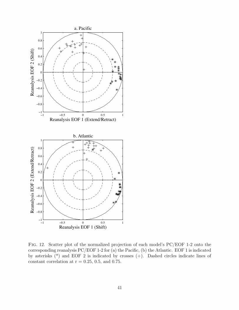
Figure 12 shows the normalized projection of the first two EOFs of each model onto the394

first two EOFs of the reanalysis data (a. Pacific, b. Atlantic). Asterisks (Crosses) indicate395

the value of the projection of EOF 1 (EOF 2) of a given model onto EOF 1 and 2 of the396

reanalysis. For instance, an asterisk located at (1,0) would describe an exemplary model’s397

depiction of EOF 1 that is completely explained by reanalysis EOF 1 and not explained by398

reanalysis EOF 2. It is important to note that the sign of a given mode is arbitrary and399

therefore the polarity is assigned based upon the convention established by reanalysis EOF400

1-2 (Fig. 2).401

Most points cluster near (0,1) or (1,0), indicating that GCMs are successfully replicating402

the two dominant modes of variability. There are only 3 outlier points: two for the Atlantic403

and one for the Pacific. The Atlantic outliers are EOF 1 and 2 from Model 1 (INGV-SXG),404

and indicate the reversal of EOF 1 and 2 in that model (not shown). Because EOF 1 and405

2 explain 15% and 14% of the variability of the Atlantic upper level winds respectively,406

this reversal is not a serious flaw in the modeled variability. For the one outlier in the407

Pacific (EOF 2 from Model 16, GISS-ER) it is found that EOF 2 and EOF 3 are reversed408

(not shown), another minor flaw since these modes explain 11% and 9% of the variability409

respectively. Therefore, all 17 models do a good job of replicating the two dominant modes410

of variability. Even the outliers have the correct structures represented in the wrong order.411

In fact, this variability appears more consistently replicated than the mean state of the jets412

in GCMs (Fig. 6).413

Because the location of the perturbation wind speeds associated with the dominant modes414

of variability is located nearby the jet exit region (see, e.g., Fig. 2), a measure of the longitude415

of the jet exit region and longitude of wind speed anomalies associated with EOF 1-2 is used416

to find a functional relationship between jet mean state and variability.417

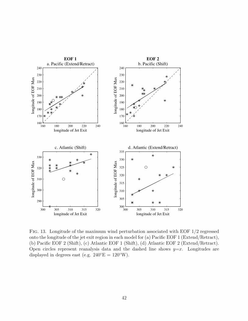
A regression analysis, shown in Fig. 13 examines the relationship between the modeled418

modes of variability and modeled mean state of the Atlantic and Pacific jets. The longitude419

of the maximum wind perturbation associated with EOF 1-2 is regressed onto the longitude420

16

of the jet exit region for each model, as defined by the local minimum of the zonal gradient421

of the mean winter zonal wind from each model. Model 16 (GISS-ER) is removed from the422

analysis of Pacific EOF 2 and Model 1 (INGV-SXG) is removed from the analysis of Atlantic423

EOF 1-2 because they do not correctly represent their respective EOFs (as shown in Fig.424

12).425

For the Pacific jet, the longitude of the maximum value of EOF 1-2 is highly correlated426

with the longitude of the jet exit region (r = 0.88, r = 0.68), shown in Fig. 13a, b (open circles427

show results from reanalysis dataset). The y = x line is also shown for the Pacific, which428

indicates the line the regression would follow if EOF 1-2 were located exactly at the longitude429

of the jet exit region. Most models correctly portray the maximum wind perturbation to be430

located immediately downstream of the jet exit region.431

Figures 13c, d show the regression analysis for the Atlantic jet, which does not display a432

similarly strong connection (r = 0.41, r = 0.43). The models all portray the maximum wind433

perturbation too far downstream for EOF 1 and most models portray the maximum wind434

perturbation too far upstream for EOF 2. Overall, there does not seem to be a link between435

the longitude of the mean state and variability for the Atlantic region, possibly because of436

the added complexity due to the southeast-northwest tilt of the jet in this region.437

There is a robust correspondence between the Pacific jet mean state and its variability,438

but not the Atlantic jet mean state and variability. When these results are repeated using439

GCM 21st century A1B projections (not shown), this correspondence (or lack thereof in440

the Atlantic) does not change. Therefore, the Pacific jet exit region is critically related to441

the longitudinal position of EOF/PC 1 and 2, signifying that a correct characterization of442

the mean state of the Pacific jet stream is vital to producing an accurate portrayal of the443

variability of that jet stream.444

17

4. Conclusions445

This study has focused on determining the reliability and robustness of non-zonally aver-446

aged NH jet stream portrayal in 17 GCMs from the CMIP3 dataset. This work is motivated447

by previous studies showing that GCM projections of 21st century jet stream winds are re-448

lated to biases in 20th century jet stream portrayal (Kidston and Gerber 2010). The results449

presented in this paper encourage targeted improvement of GCM jet stream portrayal, which450

is an important step toward assessing climate change impacts at a variety of scales.451

Examination of mean model biases of upper-level zonal winds suggests that the modeled452

Atlantic jet is too zonally extended and located too far equatorward compared to the re-453

analysis. The ensemble mean Pacific jet has less bias than the Atlantic jet, but only because454

model agreement is much lower and biases in individual models cancel in the ensemble mean.455

Mean winter biases in both basins are significant compared to the observed variability of the456

upper-level zonal winds.457

MCA and regression analysis are used in tandem to show that the NH biases in upper-458

level winds are strongly related to an ENSO-like pattern in winter mean tropical Pacific459

SSTs. Throughout the analysis we have implicitly assumed that tropical SSTs are responsi-460

ble for forcing mid-latitude winds, suggesting that the variation in models’ portrayal of the461

tropical Pacific mean state contributes to the bias of the mid-latitude large-scale circulation.462

However, it is important to note that the reverse scenario is also possible. Recent stud-463

ies have shown that variations in mid-latitude and subtropical winds may also conspire to464

produce tropical Pacific ENSO variations, as evidenced by the seasonal footprinting mech-465

anism examined in Vimont et al. (2001). It is possible that this causal mechanism (from466

mid-latitude to the tropics) would also work in linking mid-latitude wind biases to biases in467

tropical Pacific SST. While the present study does not resolve that causality, the similarity468

between the spatial structure of ENSO’s teleconnection in the observed record to the model469

bias (Fig. 6a) suggests that biases in the tropical Pacific are influencing mid-latitude zonal470

wind biases. This proposed causality is also supported by recent findings that ocean circu-471

18

lation uncertainties force uncertainties in the North Atlantic storm track in climate model472

simulations (Woollings et al. 2012).473

Temporal variability of the upper-level zonal winds is accurately modeled in nearly all474

17 GCMs. Furthermore, it is shown that in the Pacific, biases that do exist in models’475

portrayal of EOFs 1 and 2 are strongly linked to the modeled longitude of the jet exit in the476

Pacific region. This result is particularly encouraging because it implies that an improved477

characterization of the mean state of the Pacific jet will also positively impact the modeled478

variability.479

In conclusion, results herein indicate that improvements in model portrayal of the tropical480

Pacific mean state may significantly advance the portrayal of the mean state of the Pacific481

and Atlantic jets, which will consequently improve the modeled jet stream variability in482

the Pacific. To complement these findings, a second paper examines 21st century GCM483

projections of the non-zonally averaged NH jet streams. Those results show that ENSO-like484

changes in the tropical Pacific mean state dominate inter-model variations in projections of485

21st century NH jet streams.486

Acknowledgments.487

This research was supported by NSF grant ATM-0653795, NOAA grant NA08OAR4310880,488

and NSF grant ATM-0806430. NCEP Reanalysis data was provided by the NOAA/OAR/ESRL489

PSD, Boulder, Colorado, USA, from their Web site at http://www.esrl.noaa.gov/psd/. In490

addition, we acknowledge the modeling groups, the Program for Climate Model Diagnosis491

and Intercomparison (PCMDI), and the WCRP’s Working Group on Coupled Modelling492

(WGCM) for their roles in making available the WCRP CMIP3 multi-model dataset. Sup-493

port of this dataset is provided by the Office of Science, U.S. Department of Energy.494

19

495

REFERENCES496

Bengtsson, L., K. Hodges, and E. Roeckner, 2006: Storm tracks and climate change. J.497

Climate, 19 (15), 3518–3543.498

Bretherton, C., C. Smith, J. Wallace, et al., 1992: An intercomparison of methods for finding499

coupled patterns in climate data. J. Climate, 5 (6), 541–560.500

Chang, E., S. Lee, and K. Swanson, 2002: Storm track dynamics. J. Climate, 15 (16),501

2163–2183.502

Chen, G. and I. Held, 2007: Phase speed spectra and the recent poleward shift of Southern503

Hemisphere surface westerlies. Geophys. Res. Lett., 34, L21 805.504

Delworth, T., et al., 2006: GFDL’s CM2 global coupled climate models. Part I: Formulation505

and simulation characteristics. J. Climate, 19 (5), 643–674.506

Deser, C. and M. Timlin, 1997: Atmosphere-ocean interaction on weekly timescales in the507

North Atlantic and Pacific. J. Climate, 10 (3), 393–408.508

Eichelberger, S. and D. Hartmann, 2007: Zonal jet structure and the leading mode of vari-509

ability. J. Climate, 20 (20), 5149–5163.510

Flato, G., G. Boer, W. Lee, N. McFarlane, D. Ramsden, M. Reader, and A. Weaver, 2000:511

The Canadian Centre for Climate Modelling and Analysis of global coupled model and its512

climate. Clim. Dynam., 16 (6), 451–467.513

Galin, V. Y., E. M. Volodin, and S. P. Smyshliaev, 2003: Atmosphere general circulation514

model of INM RAS with ozone dynamics. Russian Meteorology and Hydrology, N (5),515

13–22.516

20

Gnanadesikan, A., et al., 2006: GFDL’s CM2 global coupled climate models. Part II: The517

baseline ocean simulation. J. Climate, 19 (5), 675–697.518

Gordon, H. et al., 2002: The CSIRO Mk3 Climate System Model. Tech. rep., CSIRO.519

Gualdi, S., E. Scoccimarro, A. Bellucci, A. Grezio, E. Manzini, and A. Navarra, 2006: The520

main features of the 20th century climate as simulated with the SXG coupled GCM. Claris521

Newsletter, none (4).522

Gualdi, S., E. Scoccimarro, A. Navarra, et al., 2008: Changes in tropical cyclone activity523

due to global warming: Results from a high-resolution coupled general circulation model.524

J. Climate, 21 (20), 5204–5228.525

Hasumi, H. and S. Emori, 2004: K-1 coupled GCM (MIROC) description. Tech. rep., Center526

for Climate System Research, University of Tokyo.527

Hu, Y., Q. Fu, et al., 2007: Observed poleward expansion of the Hadley circulation since528

1979. Atmos. Chem. and Phys., 7 (19), 5229–5236.529

Ihara, C. and Y. Kushnir, 2009: Change of mean midlatitude westerlies in 21st century530

climate simulations. Geophys. Res. Lett., 36 (13), L13 701.531

Jaffe, S., J. Martin, D. Vimont, and D. Lorenz, 2011: A synoptic climatology of episodic,532

subseasonal retractions of the Pacific jet. J. Climate, 24 (11), 2846–2860.533

Johanson, C. and Q. Fu, 2009: Hadley cell widening: Model simulations versus observations.534

J. Climate, 22 (10), 2713–2725.535

Jungclaus, J., et al., 2006: Ocean circulation and tropical variability in the coupled model536

ECHAM5/MPI-OM. J. Climate, 19 (16), 3952–3972.537

Kalnay, E., et al., 1996: The NCEP/NCAR 40-year reanalysis project. Bull. Amer. Meteor.538

Soc., 77 (3), 437–471.539

21

Karpechko, A., 2010: Uncertainties in future climate attributable to uncertainties in future540

Northern Annular Mode trend. Geophys. Res. Lett., 37 (20), L20 702.541

Kidston, J. and E. Gerber, 2010: Intermodel variability of the poleward shift of the austral542

jet stream in the CMIP3 integrations linked to biases in 20th century climatology. Geophys.543

Res. Lett., 37, L09 708.544

Kidston, J., G. Vallis, S. Dean, and J. Renwick, 2011: Can the increase in the eddy length545

scale under global warming cause the poleward shift of the jet streams? J. Climate,546

24 (14), 3764–3780.547

Kushner, P., I. Held, and T. Delworth, 2001: Southern Hemisphere atmospheric circulation548

response to global warming. J. Climate, 14, 2238–2249.549

Lorenz, D. and E. DeWeaver, 2007: Tropopause height and zonal wind response to global550

warming in the IPCC scenario integrations. J. Geophys. Res., 112 (D10), 10 119.551

Lorenz, D. and D. Hartmann, 2003: Eddy-zonal flow feedback in the Northern Hemisphere552

winter. J. Climate, 16 (8), 1212–1227.553

Lu, J., G. Vecchi, and T. Reichler, 2007: Expansion of the Hadley cell under global warming.554

Geophys. Res. Lett., 34 (1.06805).555

Lucarini, V. and G. Russell, 2002: Comparison of mean climate trends in the northern556

hemisphere between National Centers for Environmental Prediction and two atmosphere-557

ocean model forced runs. J. Geophys. Res., 107 (10.1029).558

Marshall, G., 2003: Trends in the Southern Annular Mode from observations and reanalyses.559

J. Climate, 16 (24), 4134–4143.560

Meehl, G., C. Covey, T. Delworth, M. Latif, B. McAvaney, J. Mitchell, R. Stouffer, and561

K. Taylor, 2007: The WCRP CMIP3 multi-model dataset: A new era in climate change562

research. Bull. Amer. Meteor. Soc., 88, 1383–1394.563

22

North, G., T. Bell, R. Cahalan, and F. Moeng, 1982: Sampling errors in the estimation of564

empirical orthogonal functions. Mon. Wea. Rev., 110 (7), 699–706.565

Orlanski, I., 1998: Poleward deflection of storm tracks. J. Atmos. Sci., 55 (16), 2577–2602.566

Overland, J. and M. Wang, 2005: The Arctic climate paradox: The recent decrease of the567

Arctic Oscillation. Geophys. Res. Lett., 32 (6), L06 701.568

Russell, G., J. Miller, and D. Rind, 1995: A coupled atmosphere-ocean model for transient569

climate change studies. Atmosphere-ocean, 33 (4), 683–730.570

Schmidt, G., et al., 2006: Present-day atmospheric simulations using GISS ModelE: Com-571

parison to in situ, satellite, and reanalysis data. J. Climate, 19 (2), 153–192.572

Solomon, S., 2007: Climate change 2007: the physical science basis: contribution of Working573

Group I to the Fourth Assessment Report of the Intergovernmental Panel on Climate574

Change. Cambridge Univ Pr, 996 pp.575

Thompson, D. and J. Wallace, 2000: Annular modes in the extratropical circulation. Part I:576

month-to-month variability. J. Climate, 13 (5), 1000–1016.577

Thompson, D., J. Wallace, and G. Hegerl, 2000: Annular modes in the extratropical circu-578

lation. Part II: Trends. J. Climate, 13 (5), 1018–1036.579

Ulbrich, U., J. Pinto, H. Kupfer, G. Leckebusch, T. Spangehl, and M. Reyers, 2008: Changing580

northern hemisphere storm tracks in an ensemble of IPCC climate change simulations. J.581

Climate, 21 (8), 1669–1679.582

Valdes, P. and B. Hoskins, 1989: Linear stationary wave simulations of the time-mean583

climatological flow. J. Atmos. Sci., 46, 2509–2527.584

Vimont, D., D. Battisti, and A. Hirst, 2001: Footprinting: A seasonal connection between585

the tropics and mid-latitudes. Geophys. Res. Lett., 28 (20), 3923–3926.586

23

Volodin, E. and N. Diansky, 2004: El-Nino reproduction in a coupled general circulation587

model of atmosphere and ocean. Russian Meteorology Hydrology, 12, 5–14.588

Wallace, J., C. Smith, C. Bretherton, et al., 1992: Singular value decomposition of wintertime589

sea surface temperature and 500-mb height anomalies. J. Climate, 5 (6), 561–576.590

Woollings, T., 2008: Vertical structure of anthropogenic zonal-mean atmospheric circulation591

change. Geophys. Res. Lett., 35, L19 702.592

Woollings, T. and M. Blackburn, 2012: The North Atlantic jet stream under climate change,593

and its relation to the NAO and EA patterns. J. Climate, 25 (3), 886–902.594

Woollings, T., J. Gregory, J. Pinto, M. Reyers, and D. Brayshaw, 2012: Response of the595

North Atlantic storm track to climate change shaped by ocean-atmosphere coupling. Na-596

ture Geoscience.597

Wu, Y., M. Ting, R. Seager, H. Huang, and M. Cane, 2010: Changes in storm tracks598

and energy transports in a warmer climate simulated by the GFDL CM2.1 model. Clim.599

Dynam., 37 (1), 53.600

Yaocun, Z. and H. Daqing, 2011: Has the East Asian westerly jet experienced a poleward601

displacement in recent decades? Advances in Atmospheric Sciences, 28 (6), 1259–1265.602

Yin, J., 2005: A consistent poleward shift of the storm tracks in simulations of 21st century603

climate. Geophys. Res. Lett., 32 (18), 2–5.604

Yu, Y., R. Yu, X. Zhang, and H. Liu, 2002: A flexible coupled ocean-atmosphere general605

circulation model. Advances in Atmospheric Sciences, 19 (1), 169–190.606

Yu, Y., X. Zhang, and Y. Guo, 2004: Global coupled ocean-atmosphere general circulation607

models in LASG/IAP. Advances in Atmospheric Sciences, 21 (3), 444–455.608

24

Yukimoto, S., et al., 2006: Present-day climate and climate sensitivity in the Meteorological609

Research Institute Coupled GCM Version 2.3 (MRI-CGCM2.3). J. Meteorological Society610

of Japan, 84 (2), 333–363.611

Zhang, Y., J. Wallace, and D. Battisti, 1997: ENSO-like interdecadal variability: 1900-93.612

J. Climate, 10 (5), 1004–1020.613

25

Table

1.C

MIP

3M

odel

s

Number

Model

ModelingGroup

Reference

1IN

GV

-SX

GIn

stit

uto

Naz

ion

ale

di

Geo

fisi

cae

Vu

lcan

olog

iaG

ual

di

etal

.(2

006)

and

Gu

ald

iet

al.

(200

8)

2M

IRO

C3.

2(h

ires

)C

ente

rfo

rC

lim

ate

Syst

emR

esea

rch

(th

eU

niv

ersi

tyof

Tok

yo),

Nat

ion

alIn

stit

ute

for

Envir

onm

enta

lS

tud

ies,

and

Fro

nti

erR

esea

rch

Cen

ter

for

Glo

bal

Ch

ange

(JA

MS

TE

C)

Has

um

ian

dE

mor

i(2

004)

3C

SIR

O-M

k3.

0C

omm

onw

ealt

hS

cien

tifi

can

dIn

du

stri

alR

esea

rch

Org

anis

atio

n(C

SIR

O)

Atm

osp

her

icR

esea

rch

Gor

don

etal

.(2

002)

4C

SIR

O-M

k3.

5C

omm

onw

ealt

hS

cien

tifi

can

dIn

du

stri

alR

esea

rch

Org

anis

atio

n(C

SIR

O)

Atm

osp

her

icR

esea

rch

Gor

don

etal

.(2

002)

5E

CH

AM

5/M

PI-

OM

Max

Pla

nck

Inst

itu

tefo

rM

eteo

rolo

gyJu

ngc

lau

set

al.

(200

6)

6G

FD

L-C

M2.

0U

.S.

Dep

artm

ent

ofC

omm

erce

/Nat

ion

alO

cean

ican

dA

tmos

ph

eric

Ad

min

istr

atio

n(N

OA

A)/

Geo

physi

cal

Flu

idD

yn

amic

sL

abor

ator

yD

elw

orth

etal

.(2

006)

and

Gn

anad

esik

anet

al.

(200

6)

7B

CC

R-B

CM

2.0

Bje

rkn

esC

ente

rfo

rC

lim

ate

Res

earc

hhtt

p:/

/ww

w.b

jerk

nes

.uib

.no/

8C

GC

M3.

1(T

63)

Can

adia

nC

entr

efo

rC

lim

ate

Mod

elin

gan

dA

nal

ysi

sF

lato

etal

.(2

000)

and

htt

p:/

/ww

w.e

c.gc

.ca/

ccm

ac-c

ccm

a

9C

NR

M-C

M3

Met

eo-F

ran

ce/C

entr

eN

atio

nal

de

Rec

her

ches

Met

eoro

logi

qu

eshtt

p:/

/ww

w.c

nrm

.met

eo.f

r/sc

enar

io20

04/p

aper

cm3.

pd

f

10M

IRO

C3.

2(m

edre

s)C

ente

rfo

rC

lim

ate

Syst

emR

esea

rch

(th

eU

niv

ersi

tyof

Tok

yo),

Nat

ion

alIn

stit

ute

for

Envir

onm

enta

lS

tud

ies,

and

Fro

nti

erR

esea

rch

Cen

ter

for

Glo

bal

Ch

ange

(JA

MS

TE

C)

Has

um

ian

dE

mor

i(2

004)

11M

RI-

CG

CM

2.3.

2M

eteo

rolo

gica

lR

esea

rch

Inst

itu

teY

ukim

oto

etal

.(2

006)

12F

GO

AL

S-g

1.0

Sta

teK

eyL

abor

ator

yof

Nu

mer

ical

Mod

elin

gfo

rA

tmos

ph

eric

Sci

ence

san

dG

eop

hysi

cal

Flu

idD

yn

amic

s(L

AS

G)/

Inst

itu

teof

Atm

osp

her

icP

hysi

csY

uet

al.

(200

2)an

dY

uet

al.

(200

4)

13C

GC

M3.

1(T

47)

Can

adia

nC

entr

efo

rC

lim

ate

Mod

elin

gan

dA

nal

ysi

sF

lato

etal

.(2

000)

and

htt

p:/

/ww

w.e

c.gc

.ca/

ccm

ac-c

ccm

a

14E

CH

O-G

Met

eoro

logi

cal

Inst

itu

teof

the

Un

iver

sity

ofB

onn

,M

eteo

rolo

gica

lR

esea

rch

Inst

itu

teof

KM

A,

and

Mod

elan

dD

ata

grou

phtt

p:/

/mad

.zm

aw.d

e/M

od

els/

Mod

elli

ste1

neu

.htm

l

15G

ISS

-AO

MN

AS

AG

od

dar

dIn

stit

ue

for

Sp

ace

Stu

die

sR

uss

ell

etal

.(1

995)

and

Lu

cari

ni

and

Ru

ssel

l(2

002)

16G

ISS

-ER

NA

SA

God

dar

dIn

stit

ue

for

Sp

ace

Stu

die

sS

chm

idt

etal

.(2

006)

17IN

M-C

M3.

0In

stit

ute

for

Nu

mer

ical

Mat

hem

atic

sV

olod

inan

dD

ian

sky

(200

4)an

dG

alin

etal

.(2

003)

26

List of Figures614

1 Reanalysis zonal wind (m s−1) at 300 hPa for NH winter (November-March)615

1979–1999, contoured every 10 m s−1. 30616

2 EOFs of the 300 hPa midlatitude zonal wind field (20◦–80◦N) regressed onto617

the total 300 hPa zonal wind field (0◦–80◦N). Solid (dashed) black lines repre-618

sent positive (negative) perturbation isotachs, contoured every 4 m s−1 with619

the zero line removed for (a) Pacific basin EOF 1 (Extend/Retract), (b) Pa-620

cific basin EOF 2 (Shift), (c) Atlantic basin EOF 1 (Shift), (d) Atlantic basin621

EOF 2 (Extend/Retract). Gray contours show the 20 (30) m s−1 isotach of622

the mean 300 hPa zonal wind for the Atlantic (Pacific) basins, as in Fig. 1 31623

3 Composites of maximum variability of the 300 hPa zonal wind field in the624

Atlantic. Gray contours show the 20 m s−1 isotach of the mean 300 hPa zonal625

wind for the Atlantic. Solid (dashed) black lines in the left column indicate626

positive (negative) perturbation isotachs, contoured every 5 m s1 with the627

zero line removed. The right column shows perturbation isotachs added to628

the climatology in units of m s−1 for (a)-(b) 1st principal component (PC)629

greater 1 standard deviation (1*σ), (c)-(d) 1st PC less than -1*σ, (e)-(f) 2nd630

PC greater than 1*σ, (g)-(h) 2nd PC less than -1*σ. 32631

4 (a) Ensemble mean model bias and (b) Standard deviation of models about the632

ensemble mean for the 17 GCMs under consideration [m s−1]. Solid (dashed)633

black contours in (a) represent positive (negative) values of ensemble mean634

bias, contoured every 1 m s−1 with the zero line removed. The gray contours635

show the 20, 40 m s−1 isotachs of the model mean winter 300 hPa zonal wind 33636

27

5 Solid (dashed) black contours show the positive (negative) bias of the 300637

hPa zonal wind, contoured every 4 m s−1 with the zero line removed for (a)638

Model 5: ECHAM5/MPI-OM, (b) Model 8: CGCM3.1 (T63), (c) Model 7:639

BCCR-BCM2.0, (d) Model 11: MRI-CGCM2.3.2, (e) Model 10: MIROC3.2640

(medres), (f) Model 9: CNRM-CM3. Gray contours show the 20 (30) m s−1641

isotachs of the 300 hPa zonal wind for the Atlantic (Pacific) basin. 34642

6 Normalized projection of the model bias of the 300 hPa zonal wind onto EOF643

1 and 2 from the reanalysis for the (a) Pacific and (b) Atlantic basins. Mod-644

els designated by crosses (+) are part of Group 1 and models designated by645

asterisks (*) are part of Group 2. Dashed circles indicate lines of constant646

correlation at r = 0.25, 0.5, and 0.75. The black line connects the average647

Group 1 projection to the average Group 2 projection. Open circles (dia-648

monds) show the values of the normalized projection of the heterogeneous649

wind pattern shown in Fig. 8a (ENSO teleconnection pattern shown in Fig.650

9a) onto EOF 1 and 2. 35651

7 Solid (dashed) black lines show the positive (negative) model bias of the 300652

hPa zonal wind, contoured every 1 m s−1 with the zero line removed for (Group653

2 − Group 1), where models are separated into Group 1 (models 1, 5, 7, 8,654

9, 10, 12, 13, 17) and Group 2 (models 2, 3, 4, 6, 11, 14, 15, 16), based upon655

their delineation in Figure 6, as described in the text. Gray contours show656

the 20, 40 m s−1 isotachs of the model mean 300 hPa zonal wind. 36657

8 Results of MCA of tropical Pacific SSTs and mid-latitude 300 hPa zonal658

wind. (a) Heterogeneous wind regression map, (b) Homogeneous SST regres-659

sion map, (c) Scatter plot of the wind and SST expansion coefficients. Solid660

(dashed) black contours in (a) represent positive (negative) perturbation iso-661

tachs, contoured every 1 m s−1 with the zero line removed. Gray contours in662

(a) show the 20, 30 m s−1 isotachs of the model mean 300 hPa zonal wind. 37663

28

9 ENSO mid-latitude wind teleconnection (1950-2009) shown by: (a) Observed664

mean winter 300 hPa zonal wind regressed onto the mean winter CTI and665

(b) mean winter tropical Pacific SST regressed onto the mean winter CTI.666

Solid (dashed) black contours in (a) represent positive (negative) perturbation667

isotachs, contoured every 0.5 m s−1 with the zero line removed. Gray contours668

represent the 20, 30 m s−1 isotachs of the 300 hPa mean zonal wind. 38669

10 Modeled mean winter cold tongue index (CTI) for each model regressed onto670

the modeled mean winter 300 hPa zonal wind field. Solid (dashed) black lines671

indicate positive (negative) perturbation isotachs, contoured every 1 m s−1672

with the zero line removed. Gray contours show the 20, 30 m s−1 isotachs of673

the model mean 300 hPa zonal wind. 39674

11 (a) Total inter-model variance of the mean winter 300 hPa zonal wind and (b)675

Inter-model variance of the mean winter 300 hPa zonal wind explained by the676

SST expansion coefficient of the first mode of MCA covariability. Variance is677

expressed in units of m2 s−2 and contoured every 10 m2 s−2 40678

12 Scatter plot of the normalized projection of each model’s PC/EOF 1-2 onto679

the corresponding reanalysis PC/EOF 1-2 for (a) the Pacific, (b) the Atlantic.680

EOF 1 is indicated by asterisks (*) and EOF 2 is indicated by crosses (+).681

Dashed circles indicate lines of constant correlation at r = 0.25, 0.5, and 0.75. 41682

13 Longitude of the maximum wind perturbation associated with EOF 1/2 re-683

gressed onto the longitude of the jet exit region in each model for (a) Pa-684

cific EOF 1 (Extend/Retract), (b) Pacific EOF 2 (Shift), (c) Atlantic EOF 1685

(Shift), (d) Atlantic EOF 2 (Extend/Retract). Open circles represent reanal-686

ysis data and the dashed line shows y=x. Longitudes are displayed in degrees687

east (e.g. 240◦E = 120◦W). 42688

29

1010

10

10

1010

10

30

30

30

3050

NH Mean Winter Jet (Reanalysis)

Fig. 1. Reanalysis zonal wind (m s−1) at 300 hPa for NH winter (November-March) 1979–1999, contoured every 10 m s−1.

30

a. EOF 1 (Extend/Retract) b. EOF 2 (Shift)

c. EOF 1 (Shift) d. EOF 2 (Extend/Retract)

Fig. 2. EOFs of the 300 hPa midlatitude zonal wind field (20◦–80◦N) regressed onto the total300 hPa zonal wind field (0◦–80◦N). Solid (dashed) black lines represent positive (negative)perturbation isotachs, contoured every 4 m s−1 with the zero line removed for (a) Pacificbasin EOF 1 (Extend/Retract), (b) Pacific basin EOF 2 (Shift), (c) Atlantic basin EOF 1(Shift), (d) Atlantic basin EOF 2 (Extend/Retract). Gray contours show the 20 (30) m s−1

isotach of the mean 300 hPa zonal wind for the Atlantic (Pacific) basins, as in Fig. 1

31

Anomalya. (+) EOF 1 (Shift)

c. ( ) EOF 1 (Shift)

e. (+) EOF 2 (Extend/Retract)

g. ( ) EOF 2 (Extend/Retract)

10

10 10

1010

30

3030

Full Windb. (+) EOF 1 (Shift)

10

10

10

10

30

30

d. ( ) EOF 1 (Shift)

10

10

1010

1030

30

f. (+) EOF 2 (Extend/Retract)

10

10 10

10

30

30

30

h. ( ) EOF 2 (Extend/Retract)

Fig. 3. Composites of maximum variability of the 300 hPa zonal wind field in the At-lantic. Gray contours show the 20 m s−1 isotach of the mean 300 hPa zonal wind for theAtlantic. Solid (dashed) black lines in the left column indicate positive (negative) perturba-tion isotachs, contoured every 5 m s1 with the zero line removed. The right column showsperturbation isotachs added to the climatology in units of m s−1 for (a)-(b) 1st principalcomponent (PC) greater 1 standard deviation (1*σ), (c)-(d) 1st PC less than -1*σ, (e)-(f)2nd PC greater than 1*σ, (g)-(h) 2nd PC less than -1*σ.

32

a. Ensemble Mean Bias

1 1

33

3

3

33

33

3

3

5 55 5

57 7

b. Model Standard Deviation of Bias

Fig. 4. (a) Ensemble mean model bias and (b) Standard deviation of models about theensemble mean for the 17 GCMs under consideration [m s−1]. Solid (dashed) black contoursin (a) represent positive (negative) values of ensemble mean bias, contoured every 1 m s−1

with the zero line removed. The gray contours show the 20, 40 m s−1 isotachs of the modelmean winter 300 hPa zonal wind

33

a. ECHAM5/MPI OMSmall Bias

c. BCCR BCM2.0 (Extend/Retract)EOF 1 Like Bias

e. MIROC3.2 medres (Shift)EOF 2 Like Bias

b. CGCM3.1 (T63)

d. MRI CGCM2.3.2 (Shift)

f. CNRM CM3 (Extend/Retract)

Fig. 5. Solid (dashed) black contours show the positive (negative) bias of the 300 hPa zonalwind, contoured every 4 m s−1 with the zero line removed for (a) Model 5: ECHAM5/MPI-OM, (b) Model 8: CGCM3.1 (T63), (c) Model 7: BCCR-BCM2.0, (d) Model 11: MRI-CGCM2.3.2, (e) Model 10: MIROC3.2 (medres), (f) Model 9: CNRM-CM3. Gray contoursshow the 20 (30) m s−1 isotachs of the 300 hPa zonal wind for the Atlantic (Pacific) basin.

34

1 0.5 0 0.5 11

0.8

0.6

0.4

0.2

0

0.2

0.4

0.6

0.8

1

EOF 1 Extend/Retract

EOF

2 S

hift

a. PACIFIC

1 0.5 0 0.5 11

0.8

0.6

0.4

0.2

0

0.2

0.4

0.6

0.8

1

EOF 1 Shift

EOF

2 E

xten

d/Re

tract

b. ATLANTIC

Fig. 6. Normalized projection of the model bias of the 300 hPa zonal wind onto EOF 1and 2 from the reanalysis for the (a) Pacific and (b) Atlantic basins. Models designated bycrosses (+) are part of Group 1 and models designated by asterisks (*) are part of Group 2.Dashed circles indicate lines of constant correlation at r = 0.25, 0.5, and 0.75. The black lineconnects the average Group 1 projection to the average Group 2 projection. Open circles(diamonds) show the values of the normalized projection of the heterogeneous wind patternshown in Fig. 8a (ENSO teleconnection pattern shown in Fig. 9a) onto EOF 1 and 2.

35

Grouped Model Bias

Fig. 7. Solid (dashed) black lines show the positive (negative) model bias of the 300 hPazonal wind, contoured every 1 m s−1 with the zero line removed for (Group 2 − Group 1),where models are separated into Group 1 (models 1, 5, 7, 8, 9, 10, 12, 13, 17) and Group 2(models 2, 3, 4, 6, 11, 14, 15, 16), based upon their delineation in Figure 6, as described inthe text. Gray contours show the 20, 40 m s−1 isotachs of the model mean 300 hPa zonalwind.

36

Fig. 8. Results of MCA of tropical Pacific SSTs and mid-latitude 300 hPa zonal wind. (a)Heterogeneous wind regression map, (b) Homogeneous SST regression map, (c) Scatter plotof the wind and SST expansion coefficients. Solid (dashed) black contours in (a) representpositive (negative) perturbation isotachs, contoured every 1 m s−1 with the zero line removed.Gray contours in (a) show the 20, 30 m s−1 isotachs of the model mean 300 hPa zonal wind.

37

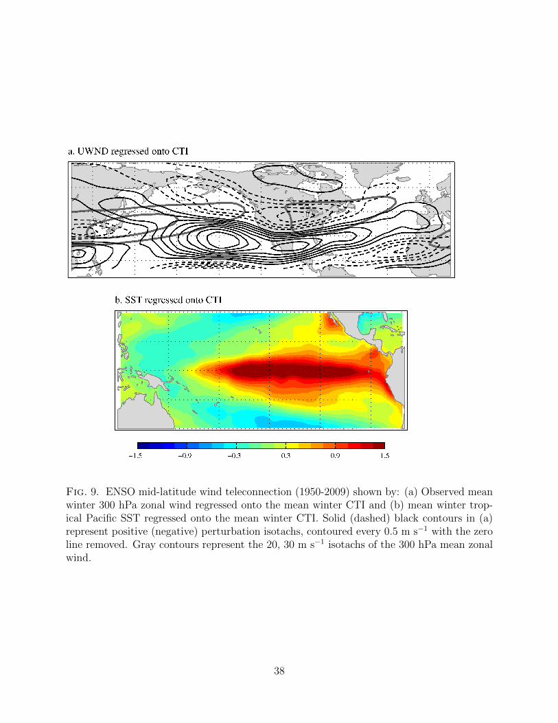
Fig. 9. ENSO mid-latitude wind teleconnection (1950-2009) shown by: (a) Observed meanwinter 300 hPa zonal wind regressed onto the mean winter CTI and (b) mean winter trop-ical Pacific SST regressed onto the mean winter CTI. Solid (dashed) black contours in (a)represent positive (negative) perturbation isotachs, contoured every 0.5 m s−1 with the zeroline removed. Gray contours represent the 20, 30 m s−1 isotachs of the 300 hPa mean zonalwind.

38

Model CTI regressed onto Model 300 hPa Zonal Wind

Fig. 10. Modeled mean winter cold tongue index (CTI) for each model regressed onto themodeled mean winter 300 hPa zonal wind field. Solid (dashed) black lines indicate positive(negative) perturbation isotachs, contoured every 1 m s−1 with the zero line removed. Graycontours show the 20, 30 m s−1 isotachs of the model mean 300 hPa zonal wind.

39

10 10

10

10

1010

10

10

1010

30

3030

3050

a. Raw Inter model Variance

10

10 1010

10

10

30

b. Variance explainted by MCA1

Fig. 11. (a) Total inter-model variance of the mean winter 300 hPa zonal wind and (b)Inter-model variance of the mean winter 300 hPa zonal wind explained by the SST expansioncoefficient of the first mode of MCA covariability. Variance is expressed in units of m2 s−2

and contoured every 10 m2 s−2

40

1 0.5 0 0.5 11

0.8

0.6

0.4

0.2

0

0.2

0.4

0.6

0.8

1

Reanalysis EOF 1 (Extend/Retract)

Rean

alys

is EO

F 2

(Shi

ft)a. Pacific

1 0.5 0 0.5 11

0.8

0.6

0.4

0.2

0

0.2

0.4

0.6

0.8

1

Reanalysis EOF 1 (Shift)

Rean

alys

is EO

F 2

(Ext

end/

Retra

ct)

b. Atlantic

Fig. 12. Scatter plot of the normalized projection of each model’s PC/EOF 1-2 onto thecorresponding reanalysis PC/EOF 1-2 for (a) the Pacific, (b) the Atlantic. EOF 1 is indicatedby asterisks (*) and EOF 2 is indicated by crosses (+). Dashed circles indicate lines ofconstant correlation at r = 0.25, 0.5, and 0.75.

41

160 180 200 220 240160

170

180

190

200

210

220

230

240

long

itude

of E

OF

Max

longitude of Jet Exit

EOF 1a. Pacific (Extend/Retract)

160 180 200 220 240160

170

180

190

200

210

220

230

240

long

itude

of E

OF

Max

longitude of Jet Exit

EOF 2b. Pacific (Shift)

300 305 310 315 320

290

300

310

320

330

long

itude

of E

OF

Max

longitude of Jet Exit

c. Atlantic (Shift)

300 305 310 315 320300

305

310

315

320

325

330

335

long

itude

of E

OF

Max

longitude of Jet Exit

d. Atlantic (Extend/Retract)

Fig. 13. Longitude of the maximum wind perturbation associated with EOF 1/2 regressedonto the longitude of the jet exit region in each model for (a) Pacific EOF 1 (Extend/Retract),(b) Pacific EOF 2 (Shift), (c) Atlantic EOF 1 (Shift), (d) Atlantic EOF 2 (Extend/Retract).Open circles represent reanalysis data and the dashed line shows y=x. Longitudes aredisplayed in degrees east (e.g. 240◦E = 120◦W).

42