2. fea and ansys - dokuz eylül Üniversitesi of... · the open ansys file icon can be used to open...

ANSYS Basics

IN

TR

OD

UC

TIO

N T

O A

NS

YS

7

.0

- P

art 1

Training Manual

November 1, 2002

Inventory #001755

3-2

• Interactive mode allows you to interact “live” with ANSYS, reviewing

each operation as you go.

• Of the three main phases of an analysis — preprocessing, solution,

postprocessing — the preprocessing and postprocessing phases are

best suited for interactive mode.

• We will mainly cover interactive mode in this course.

Interactive Mode

Overview

IN

TR

OD

UC

TIO

N T

O A

NS

YS

7

.0

- P

art 1

Training Manual

November 1, 2002

Inventory #001755

3-3

Interactive Mode

Starting ANSYS

Launcher –

• Allows you to start ANSYS and other ANSYS utilities by pressing buttons on a menu.

• On Windows systems, press:

Start > Programs > ANSYS 7.0

IN

TR

OD

UC

TIO

N T

O A

NS

YS

7

.0

- P

art 1

Training Manual

November 1, 2002

Inventory #001755

3-4

• Pressing the Interactive button on the launcher brings up a dialog

box containing start-up options:

Interactive Mode

…Starting ANSYS

Windows systems

1

2

3

4

5

IN

TR

OD

UC

TIO

N T

O A

NS

YS

7

.0

- P

art 1

Training Manual

November 1, 2002

Inventory #001755

3-5

Output

Window

Icon Toolbar Menu

Abbreviation Toolbar Menu

Utility Menu

Graphics Area

Main Menu

Input Line

The GUI

Layout

Raise/Hidden Icon

Current Settings User Prompt Info

IN

TR

OD

UC

TIO

N T

O A

NS

YS

7

.0

- P

art 1

Training Manual

November 1, 2002

Inventory #001755

3-6

• Tree structure format.

• Contains the main functions required for an

analysis.

• Use scroll bar to gain access to long tree

structures.

The GUI

Main Menu

scroll bar

IN

TR

OD

UC

TIO

N T

O A

NS

YS

7

.0

- P

art 1

Training Manual

November 1, 2002

Inventory #001755

3-7

The GUI

…Main Menu

IN

TR

OD

UC

TIO

N T

O A

NS

YS

7

.0

- P

art 1

Training Manual

November 1, 2002

Inventory #001755

3-8

Main Menu

UIDL Behavior

IN

TR

OD

UC

TIO

N T

O A

NS

YS

7

.0

- P

art 1

Training Manual

November 1, 2002

Inventory #001755

3-9

Main Menu

Filtered Branches

IN

TR

OD

UC

TIO

N T

O A

NS

YS

7

.0

- P

art 1

Training Manual

November 1, 2002

Inventory #001755

3-10

• Jobname definition when using Open ANSYS File Icon:

– the ANSYS jobname will be changed to the prefix of the database file being resumed.

Open ANSYS File

When opening the “blades.db” database

(using the Open ANSYS File Icon), the

jobname will be changed to “blades”.

The Open ANSYS File Icon can be used to open either ANSYS

Database or ANSYS Command file types

The GUI

….Icon Toolbar Menu

IN

TR

OD

UC

TIO

N T

O A

NS

YS

7

.0

- P

art 1

Training Manual

November 1, 2002

Inventory #001755

3-11

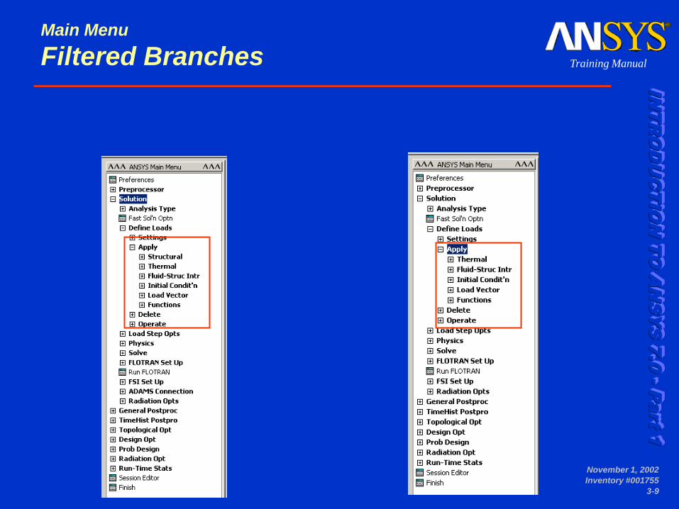
• The Preferences dialog (Main Menu >

Preferences) allows you to filter out

menu choices that are not applicable to

the current analysis.

• For example, if you are doing a thermal

analysis, you can choose to filter out

other disciplines, thereby reducing the

number of menu items available in the

GUI:

– Only thermal element types will be shown

in the element type selection dialog.

– Only thermal loads will be shown.

– Etc.

The GUI

Preferences

IN

TR

OD

UC

TIO

N T

O A

NS

YS

7

.0

- P

art 1

Training Manual

November 1, 2002

Inventory #001755

3-12

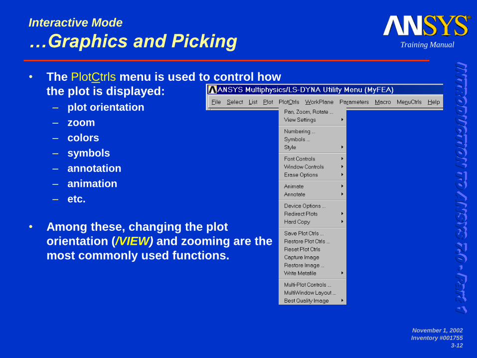
• The PlotCtrls menu is used to control how

the plot is displayed:

– plot orientation

– zoom

– colors

– symbols

– annotation

– animation

– etc.

• Among these, changing the plot

orientation (/VIEW) and zooming are the

most commonly used functions.

Interactive Mode

…Graphics and Picking

IN

TR

OD

UC

TIO

N T

O A

NS

YS

7

.0

- P

art 1

Training Manual

November 1, 2002

Inventory #001755

3-13

• The default view for a model is the front view:

looking down the +Z axis of the model.

• To change it, use dynamic mode — a way to

orient the plot dynamically using the Control

key and mouse buttons.

– Ctrl + Left mouse button pans the model.

– Ctrl + Middle mouse button:

zooms the model

spins the model (about screen Z)

– Ctrl + Right mouse button rotates the model:

about screen X

about screen Y

Note, the Shift-Right button on a two-button

mouse is equivalent to the Middle mouse

button on a three-button mouse.

P

Z R

Ctrl

Interactive Mode


IN

TR

OD

UC

TIO

N T

O A

NS

YS

7

.0

- P

art 1

Training Manual

November 1, 2002

Inventory #001755

3-14

• If you don’t want to hold down the

Control key, you can use the Dynamic

Mode setting in the Pan-Zoom-Rotate

dialog box.

– The same mouse button assignments

apply.

– On 3-D graphics devices, you can also

dynamically orient the light source.

Useful for different light source shading

effects.

Interactive Mode


When using 3-D driver

IN

TR

OD

UC

TIO

N T

O A

NS

YS

7

.0

- P

art 1

Training Manual

November 1, 2002

Inventory #001755

3-15

Picking

• Picking allows you to identify model entities

or locations by clicking in the Graphics

Window.

• A picking operation typically involves the

use of the mouse and a picker menu. It is

indicated by a + sign on the menu.

• For example, you can create keypoints by

picking locations in the Graphics Window

and then pressing OK in the picker.

Interactive Mode


IN

TR

OD

UC

TIO

N T

O A

NS

YS

7

.0

- P

art 1

Training Manual

November 1, 2002

Inventory #001755

3-16

• The term ANSYS database refers to the data ANSYS maintains in

memory as you build, solve, and postprocess your model.

• The database stores both your input data and ANSYS results data:

– Input data -- information you must enter, such as model dimensions,

material properties, and load data.

– Results data -- quantities that ANSYS calculates, such as

displacements, stresses, strains, and reaction forces.

Interactive Mode

The Database and Files

IN

TR

OD

UC

TIO

N T

O A

NS

YS

7

.0

- P

art 1

Training Manual

November 1, 2002

Inventory #001755

3-17

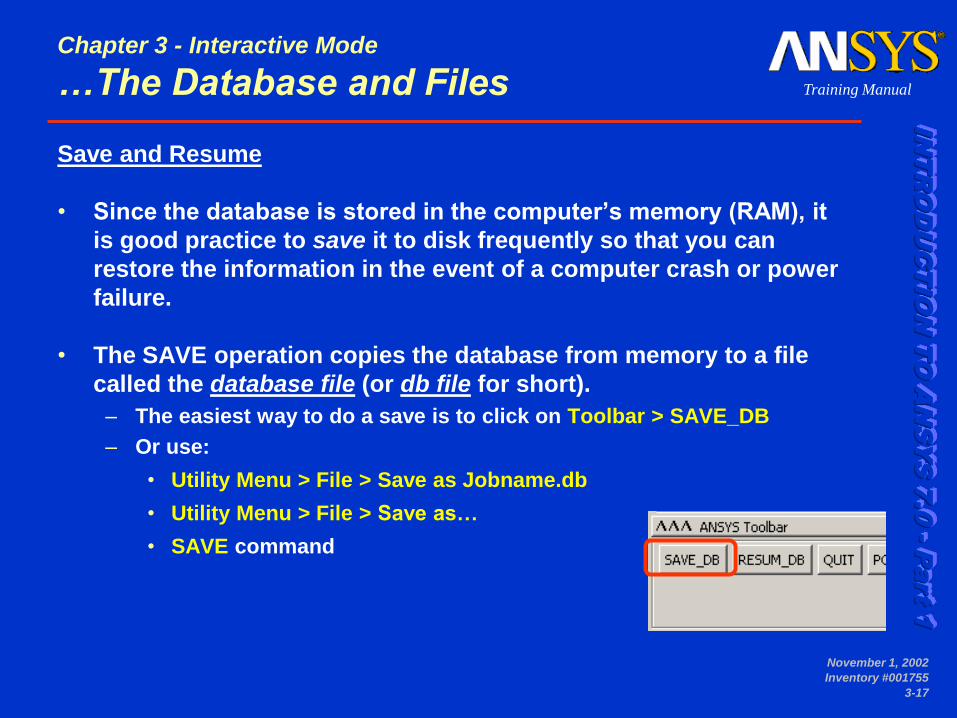
Save and Resume

• Since the database is stored in the computer’s memory (RAM), it

is good practice to save it to disk frequently so that you can

restore the information in the event of a computer crash or power

failure.

• The SAVE operation copies the database from memory to a file

called the database file (or db file for short).

– The easiest way to do a save is to click on Toolbar > SAVE_DB

– Or use:

• Utility Menu > File > Save as Jobname.db

• Utility Menu > File > Save as…

• SAVE command

Chapter 3 - Interactive Mode

…The Database and Files

IN

TR

OD

UC

TIO

N T

O A

NS

YS

7

.0

- P

art 1

Training Manual

November 1, 2002

Inventory #001755

3-18

• To restore the database from the db file back into memory, use the

RESUME operation.

– Toolbar > RESUME_DB

– Or use:

• Utility Menu > File > Resume Jobname.db

• Utility Menu > File > Resume from…

• RESUME command

• The default file name for SAVE and RESUME is jobname.db, but

you can choose a different name by using the “Save as” or

“Resume from” functions.



IN

TR

OD

UC

TIO

N T

O A

NS

YS

7

.0

- P

art 1

Training Manual

November 1, 2002

Inventory #001755

3-19

Clearing the Database

• The Clear Database operation allows

you to “zero out” the database and

start fresh. It is similar to exiting and

re-entering ANSYS.

– Utility Menu > File > Clear & Start New

– Or use the /CLEAR command.



IN

TR

OD

UC

TIO

N T

O A

NS

YS

7

.0

- P

art 1

Training Manual

November 1, 2002

Inventory #001755

3-20

• Typical files:

jobname.log: Log file, ASCII.

• Contains a log of every command issued during the session.

• If you start a second session with the same jobname in the same

working directory, ANSYS will append to the previous log file (with

a time stamp).

jobname.err: Error file, ASCII.

• Contains all errors and warnings encountered during the session.

ANSYS will also append to an existing error file.

jobname.db, .dbb: Database file, binary.

• Compatible across all supported platforms.

jobname.rst, .rth, .rmg, .rfl: Results files, binary.

• Contains results data calculated by ANSYS during solution.

• Compatible across all supported platforms.



IN

TR

OD

UC

TIO

N T

O A

NS

YS

7

.0

- P

art 1

Training Manual

November 1, 2002

Inventory #001755

3-21

File Management Tips

• Run each analysis project in a separate working directory.

• Use different jobnames to differentiate various analysis runs.

• You should keep the following files after any ANSYS analysis:

– log file ( .log)

– database file ( .db)

– results files (.rst, .rth, …)

– load step files, if any (.s01, .s02, ...)

– physics files (.ph1, .ph2, ...)

• Use /FDELETE or Utility Menu > File > ANSYS File Options to

automatically delete files no longer needed by ANSYS during that

session.



IN

TR

OD

UC

TIO

N T

O A

NS

YS

7

.0

- P

art 1

Training Manual

November 1, 2002

Inventory #001755

3-22

• Three ways to exit ANSYS:

– Toolbar > QUIT

– Utility Menu > File > Exit

– Use the /EXIT command in the Input Window


Exiting ANSYS

IN

TR

OD

UC

TIO

N T

O A

NS

YS

7

.0

- P

art 1

Training Manual

November 1, 2002

Inventory #001755

4-23

Every analysis involves four main steps:

• Preliminary Decisions

– Which analysis type?

– What to model?

– Which element type?

• Preprocessing

– Define Material

– Create or import the model geometry

– Mesh the geometry

• Solution

– Apply loads

– Solve

• Postprocessing

– Review results

– Check the validity of the solution

Preprocessing

Solution

Postprocessing

Preliminary

Decisions

Chapter 4 - General Analysis Procedure

…Overview

IN

TR

OD

UC

TIO

N T

O A

NS

YS

7

.0

- P

art 1

Training Manual

November 1, 2002

Inventory #001755

4-24

Chapter 4 - A. Preliminary Decisions

Which analysis type?

• The analysis type usually belongs to one of the following

disciplines:

Structural Motion of solid bodies, pressure on solid bodies, or

contact of solid bodies

Thermal Applied heat, high temperatures, or changes in

temperature

Electromagnetic Devices subjected to electric currents (AC or DC),

electromagnetic waves, and voltage or charge

excitation

Fluid Motion of gases/fluids, or contained gases/fluids

Coupled-Field Combinations of any of the above

•The appropriate analysis type for this model is a structural analysis!

IN

TR

OD

UC

TIO

N T

O A

NS

YS

7

.0

- P

art 1

Training Manual

November 1, 2002

Inventory #001755

4-25


…What to model?

• What should be used to model the geometry of the spherical tank?

– Axisymmetry since the loading, material, and the boundary

conditions are symmetric. This type of model would provide the

most simplified model.

– Rotational symmetry since the loading, material, and the

boundary conditions are symmetric. Advantage over

axisymmetry: offers some results away from applied boundary

conditions.

– Full 3D model is an option, but would not be an efficient choice

compared to the axisymmetric and quarter symmetry models. If

model results are significantly influenced by symmetric

boundary conditions, this may be the only option.

An axisymmetric and a one-quarter symmetry (i.e. rotational

symmetry) model will be analyzed for this model!

IN

TR

OD

UC

TIO

N T

O A

NS

YS

7

.0

- P

art 1

Training Manual

November 1, 2002

Inventory #001755

4-26


…Which Element Type?

• What element type should be used for the model of the spherical

tank?

– Axisymmetric model:

• Axisymmetric since 2-D section can be revolved to created 3D

geometry.

• Linear due to small displacement assumption.

– PLANE42 with KEYOPT(3) = 1

– Rotational symmetry model:

• Shell since radius/thickness ratio > 10

• Linear due to small displacement assumption.

• membrane stiffness only option since “membrane stresses” are

required.

– SHELL63 with KEYOPT(1) = 1

• Since the meshing of this geometry will create SHELL63 elements

with shape warnings, a mid-side noded equation of the SHELL63 was

used:

– SHELL93 with KEYOPT(1) = 1

IN

TR

OD

UC

TIO

N T

O A

NS

YS

7

.0

- P

art 1

Training Manual

November 1, 2002

Inventory #001755

4-27

• A typical solid model is defined by volumes, areas, lines, and

keypoints.

– Volumes are bounded by areas. They represent solid objects.

– Areas are bounded by lines. They represent faces of solid objects, or

planar or shell objects.

– Lines are bounded by keypoints. They represent edges of objects.

– Keypoints are locations in 3-D space. They represent vertices of

objects.

Volumes Areas Lines & Keypoints

Chapter 4 - B. Preprocessing

…Create the Solid Model

IN

TR

OD

UC

TIO

N T

O A

NS

YS

7

.0

- P

art 1

Training Manual

November 1, 2002

Inventory #001755

4-28

• Meshing is the process used to “fill” the solid model with nodes

and elements, i.e, to create the FEA model.

– Remember, you need nodes and elements for the finite element

solution, not just the solid model. The solid model does NOT

participate in the finite element solution.

Solid model FEA model

meshing


Create the FEA Model

IN

TR

OD

UC

TIO

N T

O A

NS

YS

7

.0

- P

art 1

Training Manual

November 1, 2002

Inventory #001755

4-29


Define Material

Material Properties

• Every analysis requires some material property input: Young’s

modulus EX for structural elements, thermal conductivity KXX for

thermal elements, etc.

• There are two ways to define material properties:

– Material library

– Individual properties

IN

TR

OD

UC

TIO

N T

O A

NS

YS

7

.0

- P

art 1

Training Manual

November 1, 2002

Inventory #001755

4-30

• There are five categories of loads:

DOF Constraints Specified DOF values, such as displacements

in a stress analysis or temperatures in a

thermal analysis.

Concentrated Loads Point loads, such as forces or heat flow rates.

Surface Loads Loads distributed over a surface, such as

pressures or convections.

Body Loads Volumetric or field loads, such as temperatures

(causing thermal expansion) or internal heat

generation.

Inertia Loads Loads due to structural mass or inertia, such

as gravity and rotational velocity.

Chapter 4 – C. Solution

Define Loads

IN

TR

OD

UC

TIO

N T

O A

NS

YS

7

.0

- P

art 1

Training Manual

November 1, 2002

Inventory #001755

4-31

• Postprocessing is the final step in the finite element analysis

process.

• It is imperative that you interpret your results relative to the

assumptions made during model creation and solution.

• You may be required to make design decisions based on the

results, so it is a good idea not only to review the results carefully,

but also to check the validity of the solution.

• ANSYS has two postprocessors:

– POST1, the General Postprocessor, to review a single set of results

over the entire model.

– POST26, the Time-History Postprocessor, to review results at selected

points in the model over time. Mainly used for transient and nonlinear

analyses. (Not discussed in this course.)

Chapter 4 - D. Postprocessing

Review Results

Creating the Solid Model

Chapter 5

IN

TR

OD

UC

TIO

N T

O A

NS

YS

7

.0

- P

art 1

Training Manual

November 1, 2002

Inventory #001755

5-33

Details

• Small details that are unimportant to the analysis should not be

included in the analysis model. You can suppress such features

before sending a model to ANSYS from a CAD system.

• For some structures, however, "small" details such as fillets or

holes can be locations of maximum stress and might be quite

important, depending on your analysis objectives.

Chapter 5 – A. What to Model

…What to model?

IN

TR

OD

UC

TIO

N T

O A

NS

YS

7

.0

- P

art 1

Training Manual

November 1, 2002

Inventory #001755

5-34

Symmetry

• Many structures are symmetric in some form and allow only a

representative portion or cross-section to be modeled.

• The main advantages of using a symmetric model are:

– It is generally easier to create the model.

– It allows you to make a finer, more detailed model and thereby obtain

better results than would have been possible with the full model.


…What to model?

IN

TR

OD

UC

TIO

N T

O A

NS

YS

7

.0

- P

art 1

Training Manual

November 1, 2002

Inventory #001755

5-35

• To take advantage of symmetry, all of the following must be

symmetric:

– Geometry

– Material properties

– Loading conditions

• There are different types of symmetry:

– Axisymmetry

– Rotational

– Planar or reflective

– Repetitive or translational


…What to model?

IN

TR

OD

UC

TIO

N T

O A

NS

YS

7

.0

- P

art 1

Training Manual

November 1, 2002

Inventory #001755

5-36

Axisymmetry

• Symmetry about a central axis, such as in light bulbs, straight

pipes, cones, circular plates, and domes.

• Plane of symmetry is the cross-section anywhere around the

structure. Thus you are using a single 2-D “slice” to represent

360° — a real savings in model size!

• Loading is also assumed to be

axisymmetric in most cases. However,

if it is not, and if the analysis is linear,

the loads can be separated into

harmonic components for independent

solutions that can be superimposed.


…What to model?

IN

TR

OD

UC

TIO

N T

O A

NS

YS

7

.0

- P

art 1

Training Manual

November 1, 2002

Inventory #001755

5-37

Rotational symmetry

• Repeated segments arranged about a central axis, such as in

turbine rotors.

• Only one segment of the structure needs to be modeled.

• Loading is also assumed to be symmetric about the axis.


…What to model?

IN

TR

OD

UC

TIO

N T

O A

NS

YS

7

.0

- P

art 1

Training Manual

November 1, 2002

Inventory #001755

5-38

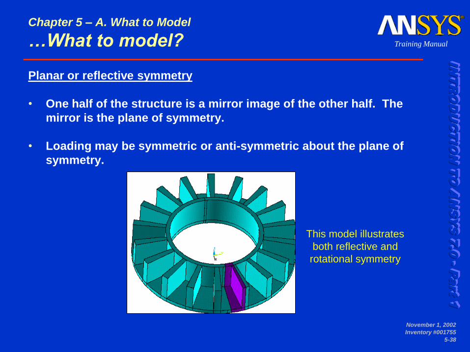
This model illustrates

both reflective and

rotational symmetry

Planar or reflective symmetry

• One half of the structure is a mirror image of the other half. The

mirror is the plane of symmetry.

• Loading may be symmetric or anti-symmetric about the plane of

symmetry.


…What to model?

IN

TR

OD

UC

TIO

N T

O A

NS

YS

7

.0

- P

art 1

Training Manual

November 1, 2002

Inventory #001755

5-39

This model illustrates both repetitive and reflective symmetry.

Repetitive or translational symmetry

• Repeated segments arranged along a straight line, such as a long

pipe with evenly spaced cooling fins.

• Loading is also assumed to be “repeated” along the length of the

model.


…What to model?

IN

TR

OD

UC

TIO

N T

O A

NS

YS

7

.0

- P

art 1

Training Manual

November 1, 2002

Inventory #001755

5-40

• In some cases, only a few minor details will disrupt a structure's

symmetry. You may be able to ignore such details (or treat them

as being symmetric) in order to gain the benefits of using a

smaller model. How much accuracy is lost as the result of such a

compromise might be difficult to estimate.


…What to model?

IN

TR

OD

UC

TIO

N T

O A

NS

YS

7

.0

- P

art 1

Training Manual

November 1, 2002

Inventory #001755

5-41

• Solid Modeling can be defined as the process of

creating solid models.

• Definitions:

– A solid model is defined by volumes, areas, lines,

and keypoints.

– Volumes are bounded by areas, areas by lines, and

lines by keypoints.

– Hierarchy of entities from low to high:

keypoints < lines < areas < volumes

– You cannot delete an entity if a higher-order entity

is attached to it.

• Also, a model with just areas and below, such as

a shell or 2-D plane model, is still considered a

solid model in ANSYS terminology.

Volumes

Areas

Lines &

Keypoints

Keypoints

Lines

Areas

Volumes

Chapter 5 – C. ANSYS Native Commands

Definitions

Create Finite Element Model

Chapter 6

IN

TR

OD

UC

TIO

N T

O A

NS

YS

7

.0

- P

art 1

Training Manual

November 1, 2002

Inventory #001755

6-43

Chapter 6 – Creating the Finite Element Model

Overview

• The purpose of this chapter is to discuss the meshing element

attributes, various means to create a mesh in ANSYS, and finally

how to import one’s finite element model directly into ANSYS.

Recall, ANSYS does not use the solid model in the solution of the

model, rather it needs to use finite elements.

IN

TR

OD

UC

TIO

N T

O A

NS

YS

7

.0

- P

art 1

Training Manual

November 1, 2002

Inventory #001755

6-44

• Meshing is the process used to “fill” the solid model with nodes

and elements, i.e, to create the FEA model.

– Remember, you need nodes and elements for the finite element

solution, not just the solid model. The solid model does NOT

participate in the finite element solution.

Solid model FEA model

meshing


…Overview

IN

TR

OD

UC

TIO

N T

O A

NS

YS

7

.0

- P

art 1

Training Manual

November 1, 2002

Inventory #001755

6-45

• There are three steps to meshing:

– Define element attributes

– Specify mesh controls

– Generate the mesh

• Element attributes are characteristics of the finite element model

that you must establish prior to meshing. They include:

– Element types

– Real constants

– Material properties


Element Attributes

IN

TR

OD

UC

TIO

N T

O A

NS

YS

7

.0

- P

art 1

Training Manual

November 1, 2002

Inventory #001755

6-46

Element Type

• The element type is an important choice that determines the

following element characteristics:

– Degree of Freedom (DOF) set. A thermal element type, for example,

has one dof: TEMP, whereas a structural element type may have up to

six dof: UX, UY, UZ, ROTX, ROTY, ROTZ.

– Element shape -- brick, tetrahedron, quadrilateral, triangle, etc.

– Dimensionality -- 2-D (X-Y plane only), or 3-D.

– Assumed displacement shape -- linear vs. quadratic.

• ANSYS has a “library” of over 150 element types from which you

can choose. Details on how to choose the “correct” element type

will be presented later. For now, let’s see how to define an

element type.


…Element Attributes

IN

TR

OD

UC

TIO

N T

O A

NS

YS

7

.0

- P

art 1

Training Manual

November 1, 2002

Inventory #001755

6-47

Element category

• ANSYS offers many different categories of elements. Some of the

commonly used ones are:

– Line elements

– Shells

– 2-D solids

– 3-D solids



IN

TR

OD

UC

TIO

N T

O A

NS

YS

7

.0

- P

art 1

Training Manual

November 1, 2002

Inventory #001755

6-48

• Line elements:

– Beam elements are used to model bolts, tubular members, C-sections,

angle irons, or any long, slender members where only membrane and

bending stresses are needed.

– Spar elements are used to model springs, bolts, preloaded bolts, and

truss members.

– Spring elements are used to model springs, bolts, or long slender

parts, or to replace complex parts by an equivalent stiffness.



IN

TR

OD

UC

TIO

N T

O A

NS

YS

7

.0

- P

art 1

Training Manual

November 1, 2002

Inventory #001755

6-49

• Shell elements:

– Used to model thin panels or curved surfaces.

– The definition of “thin” depends on the application, but as a general

guideline, the major dimensions of the shell structure (panel) should

be at least 10 times its thickness.



IN

TR

OD

UC

TIO

N T

O A

NS

YS

7

.0

- P

art 1

Training Manual

November 1, 2002

Inventory #001755

6-50

• 2-D Solid elements:

– Used to model a cross-section of solid objects.

– Must be modeled in the global Cartesian X-Y plane.

– All loads are in the X-Y plane, and the response (displacements) are

also in the X-Y plane.

– Element behavior may be one of the following:

• plane stress

• plane strain

• generalized plain strain

• axisymmetric

• axisymmetric harmonic

Y

X Z



IN

TR

OD

UC

TIO

N T

O A

NS

YS

7

.0

- P

art 1

Training Manual

November 1, 2002

Inventory #001755

6-51

• Plane stress assumes zero stress in

the Z direction.

– Valid for components in which the Z

dimension is smaller than the X and Y

dimensions.

– Z-strain is non-zero.

– Optional thickness (Z direction)

allowed.

– Used for structures such as flat plates

subjected to in-plane loading, or thin

disks under pressure or centrifugal

loading.

Y

X Z



IN

TR

OD

UC

TIO

N T

O A

NS

YS

7

.0

- P

art 1

Training Manual

November 1, 2002

Inventory #001755

6-52

• Plane strain assumes zero strain in the Z

direction.

– Valid for components in which the Z dimension is

much larger than the X and Y dimensions.

– Z-stress is non-zero.

– Used for long, constant cross-section structures

such as structural beams.

Y X

Z



IN

TR

OD

UC

TIO

N T

O A

NS

YS

7

.0

- P

art 1

Training Manual

November 1, 2002

Inventory #001755

6-53



• Generalized Plane Strain assumes a finite deformation domain

length in the Z direction, as opposed to the infinite value assumed

for standard plane strain.

– Gives more practical results for deformation problems where the Z-

direction dimension is not long enough.

– Gives users a more efficient way to simulate certain 3-D deformations

using 2-D element options.

– Option is a feature developed for PLANE182 and PLANE183.

– The deformation domain or structure

is formed by extruding a plane area

along a curve with a constant curvature.

IN

TR

OD

UC

TIO

N T

O A

NS

YS

7

.0

- P

art 1

Training Manual

November 1, 2002

Inventory #001755

6-54

• Axisymmetry assumes that the 3-D model and its

loading can be generated by revolving a 2-D

section 360° about the Y axis.

– Axis of symmetry must coincide with the global Y

axis.

– Negative X coordinates are not permitted.

– Y direction is axial, X direction is radial, and Z

direction is circumferential (hoop) direction.

– Hoop displacement is zero; hoop strains and

stresses are usually very significant.

– Used for pressure vessels, straight pipes, shafts,

etc.



IN

TR

OD

UC

TIO

N T

O A

NS

YS

7

.0

- P

art 1

Training Manual

November 1, 2002

Inventory #001755

6-55

• Axisymmetric harmonic is a special case of axisymmetry where

the loads can be non-axisymmetric.

– The non-axisymmetric loading is decomposed into Fourier series

components, applied and solved separately, and then combined later.

No approximation is introduced by this simplification!

– Used for non-axisymmetric loads such as torque on a shaft.



IN

TR

OD

UC

TIO

N T

O A

NS

YS

7

.0

- P

art 1

Training Manual

November 1, 2002

Inventory #001755

6-56

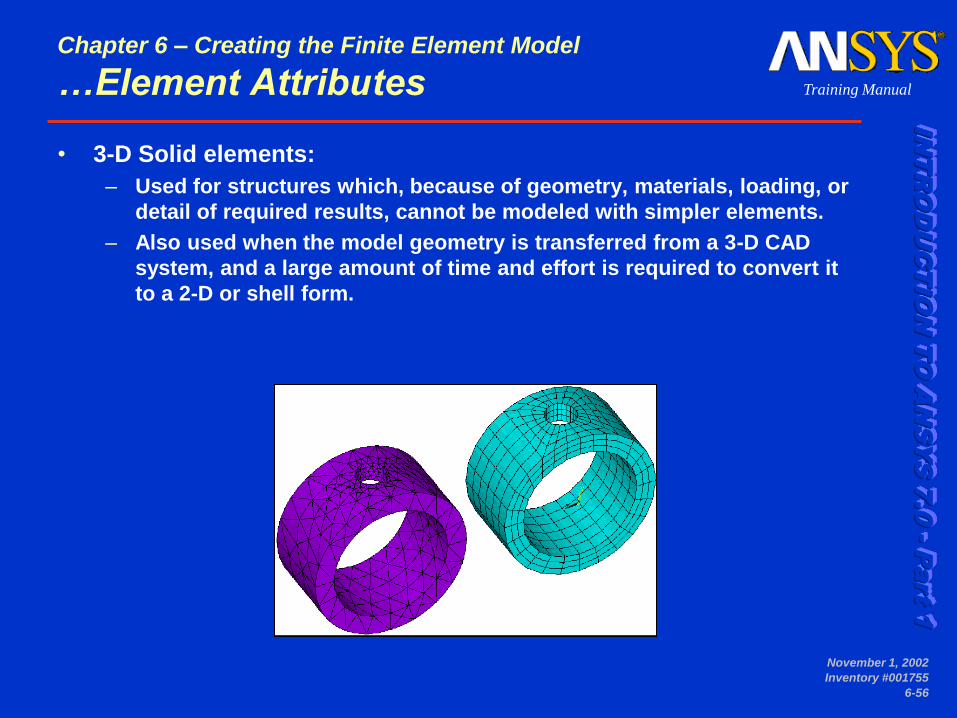
• 3-D Solid elements:

– Used for structures which, because of geometry, materials, loading, or

detail of required results, cannot be modeled with simpler elements.

– Also used when the model geometry is transferred from a 3-D CAD

system, and a large amount of time and effort is required to convert it

to a 2-D or shell form.



IN

TR

OD

UC

TIO

N T

O A

NS

YS

7

.0

- P

art 1

Training Manual

November 1, 2002

Inventory #001755

6-57

• To define an element type:

– Main Menu > Preprocessor >

Element Type > Add/Edit/Delete

• [Add] to add new element type

• Choose the desired type

(such as SOLID92) and press

OK

• [Options] to specify additional

element options

– Or use the ET command:

• et,1,solid92



IN

TR

OD

UC

TIO

N T

O A

NS

YS

7

.0

- P

art 1

Training Manual

November 1, 2002

Inventory #001755

6-58

• Notes:

– Setting preferences to the desired discipline (Main Menu > Preferences)

will show only the element types valid for that discipline.

– You should define the element type early in the preprocessing phase

because many of the menu choices in the GUI are filtered out based

on the current DOF set. For example, if you choose a structural

element type, thermal load choices will not be not shown at all.



IN

TR

OD

UC

TIO

N T

O A

NS

YS

7

.0

- P

art 1

Training Manual

November 1, 2002

Inventory #001755

6-59

Real Constants

• Real constants are used for geometric properties that cannot be

completely defined by the element’s geometry. For example:

– A beam element is defined by a line joining two nodes. This defines

only the length of the beam. To specify the beam’s cross-sectional

properties, such as the area and moment of inertia, you need to use

real constants.

– A shell element is defined by a quadrilateral or triangular area. This

defines only the surface area of the shell. To specify the shell

thickness, you need to use real constants.

– Most 3-D solid elements do not require a real constant since the

element geometry is fully defined by its nodes.



IN

TR

OD

UC

TIO

N T

O A

NS

YS

7

.0

- P

art 1

Training Manual

November 1, 2002

Inventory #001755

6-60

• To define real constants:

– Main Menu > Preprocessor > Real

Constants

• [Add] to add a new real constant

set.

• If multiple element types have

been defined, choose the element

type for which you are specifying

real constants.

• Then enter the real constant

values.

– Or use the R family of commands.

• Different element types require

different real constants. Check the

Elements Manual, available on-line,

for details.



IN

TR

OD

UC

TIO

N T

O A

NS

YS

7

.0

- P

art 1

Training Manual

November 1, 2002

Inventory #001755

6-61

Material Properties

• Every analysis requires some material property input: Young’s

modulus EX for structural elements, thermal conductivity KXX for

thermal elements, etc.

• Refer to Chapter 7 for details on the two ways to define material

properties.



IN

TR

OD

UC

TIO

N T

O A

NS

YS

7

.0

- P

art 1

Training Manual

November 1, 2002

Inventory #001755

6-62

• Most FEA models have multiple attributes. For example, the silo shown

here has two element types, three real constant sets, and two materials.

MAT 1 = concrete

MAT 2 = steel

REAL 1 = 3/8” thickness

REAL 2 = beam properties

REAL 3 = 1/8” thickness

TYPE 1 = shell

TYPE 2 = beam


Multiple Element Attributes

IN

TR

OD

UC

TIO

N T

O A

NS

YS

7

.0

- P

art 1

Training Manual

November 1, 2002

Inventory #001755

6-63

• Whenever you have multiple TYPEs, REALs and MATs, you need

to make sure that each element is assigned the proper attributes.

There are three ways to do this:

– Assign attributes to the solid model entities before meshing

– Activate a “global” setting of MAT, TYPE, and REAL before meshing

– Modify element attributes after meshing

• If no assignments are made, ANSYS uses default settings of

MAT=1, TYPE=1, and REAL=1 for all elements in the model. Note,

the current active TYPE, REAL, and MAT dictates mesh operation.


…Multiple Element Attributes

IN

TR

OD

UC

TIO

N T

O A

NS

YS

7

.0

- P

art 1

Training Manual

November 1, 2002

Inventory #001755

6-64

Modifying Element Attributes

1. Define all necessary element types, materials, and real constant sets.

2. Activate the desired combination of TYPE, REAL, and MAT settings:

– Main Menu > Preprocessor > Meshing > Mesh Attributes > Default Attribs

– Or use the TYPE, REAL, and MAT commands

3. Modify the attributes of only those elements to which the above settings apply:

– Issue EMODIF,PICK or choose Main Menu > Preprocessor > Modeling > Move/Modify > Elements > Modify Attrib

– Then pick the desired elements

4. In the subsequent dialog box, set attributes to “All to current.”


…Multiple Element Attributes

IN

TR

OD

UC

TIO

N T

O A

NS

YS

7

.0

- P

art 1

Training Manual

November 1, 2002

Inventory #001755

6-65

• Examples of different SmartSize

levels are shown here for a

tetrahedron mesh.

• Advanced SmartSize controls, such

as mesh expansion and transition

factors, are available on the SMRT

command or:

Main Menu > Preprocessor > Meshing >

Size Cntrls > SmartSize > Adv Opts

• You can turn off SmartSizing using

the MeshTool or by issuing smrt,off.


…Controlling Mesh Density

IN

TR

OD

UC

TIO

N T

O A

NS

YS

7

.0

- P

art 1

Training Manual

November 1, 2002

Inventory #001755

6-66

• There are two main meshing methods: free and

mapped.

• Free Mesh

– Has no element shape restrictions.

– The mesh does not follow any pattern.

– Suitable for complex shaped areas and volumes.

• Mapped Mesh

– Restricts element shapes to quadrilaterals for areas

and hexahedra (bricks) for volumes.

– Typically has a regular pattern with obvious rows of

elements.

– Suitable only for “regular” areas and volumes such as

rectangles and bricks.


Mapped Meshing

IN

TR

OD

UC

TIO

N T

O A

NS

YS

7

.0

- P

art 1

Training Manual

November 1, 2002

Inventory #001755

6-67

• For volume meshing, we have only seen two

options so far:

– Free meshing, which creates an all-tet mesh. This

is easy to achieve but may not be desirable in

some cases because of the large number of

elements and total DOF created.

– Mapped meshing, which creates an all-hex mesh.

This is desirable but usually very difficult to

achieve.

• Hex-to-tet meshing provides a third option that

is the “best of both worlds.” It allows you to

have a combination of hex and tet meshes

without compromising the integrity of the mesh.


Hex-to-Tet Meshing

IN

TR

OD

UC

TIO

N T

O A

NS

YS

7

.0

- P

art 1

Training Manual

November 1, 2002

Inventory #001755

6-68

• This option works by creating pyramid-shaped elements in the transition

region between hex and tet regions.

– Requires the hex mesh to be available (or at least a quad mesh at the shared

area).

– The mesher first creates all tets, then combines and rearranges the tet elements

in the transition region to form pyramids.

– Available only for element types that support both pyramid and tet shapes, e.g:

• Structural SOLID95, 186, VISCO89

• Thermal SOLID90

• Multiphysics SOLID62, 117, 122

SOLID95

– Results are good even in the transition

region. Element faces are compatible even

when transitioning from a linear hex

element to a quadratic tet element.


…Hex-to-Tet Meshing

IN

TR

OD

UC

TIO

N T

O A

NS

YS

7

.0

- P

art 1

Training Manual

November 1, 2002

Inventory #001755

6-69

– Hex-to-tet meshing is valid for both quadratic-to-quadratic and linear-to-

quadratic transitions. Element type must support a 9-node pyramid for the latter.

8-Node Hex 9-Node Pyramid 10-Node Tet

Hex Mesh Transition Layer Tet Mesh

Quadratic

to

Quadratic

Linear

to

Quadratic

10-Node Tet 13-Node Pyramid 20-Node Hex


…Hex-to-Tet Meshing

Defining the Material

Chapter 7

IN

TR

OD

UC

TIO

N T

O A

NS

YS

7

.0

- P

art 1

Training Manual

November 1, 2002

Inventory #001755

7-71

Specifying Individual Material Properties

• Instead of choosing a material name, this method involves directly

specifying the required properties through the Material Model GUI.

• To specify individual

properties:

– Main Menu > Preprocessor >

Material Props > Material Models

• Double-click on the

appropriate property to be

defined.

Chapter 7 – Defining the Material

Material Model GUI

IN

TR

OD

UC

TIO

N T

O A

NS

YS

7

.0

- P

art 1

Training Manual

November 1, 2002

Inventory #001755

7-72

• Work through the tree

structure to the material

type to be defined.

• Then enter the individual

property values.

• Or use the MP command. – mp,ex,1,30e6

– mp,prxy,1,.3


…Material Model GUI

IN

TR

OD

UC

TIO

N T

O A

NS

YS

7

.0

- P

art 1

Training Manual

November 1, 2002

Inventory #001755

7-73

• Add temperature dependent

properties

• Graph properties vs. temperature


…Material Model GUI

Loading

Chapter 8

IN

TR

OD

UC

TIO

N T

O A

NS

YS

7

.0

- P

art 1

Training Manual

November 1, 2002

Inventory #001755

8-75

• The solution step is where we apply loads on the object and let

the solver calculate the finite element solution.

• Loads are available both in the Solution and Preprocessor menus.

Chapter 8 - Loading

Overview

IN

TR

OD

UC

TIO

N T

O A

NS

YS

7

.0

- P

art 1

Training Manual

November 1, 2002

Inventory #001755

8-76

• There are five categories of loads:

DOF Constraints Specified DOF values, such as displacements

in a stress analysis or temperatures in a

thermal analysis.

Concentrated Loads Point loads, such as forces or heat flow rates.

Surface Loads Loads distributed over a surface, such as

pressures or convections.

Body Loads Volumetric or field loads, such as temperatures

(causing thermal expansion) or internal heat

generation.

Inertia Loads Loads due to structural mass or inertia, such

as gravity and rotational velocity.

Chapter 8 - Loading

Define Loads

IN

TR

OD

UC

TIO

N T

O A

NS

YS

7

.0

- P

art 1

Training Manual

November 1, 2002

Inventory #001755

8-77

• You can apply loads either on the solid model or directly on the

FEA model (nodes and elements).

– Solid model loads are easier to apply because there are fewer entities

to pick.

– Moreover, solid model loads are independent of the mesh. You don’t

need to reapply the loads if you change the mesh.

Constraints

at nodes

FEA model

Pressures on element faces

Force at node

Constraint

on line

Solid model

Pressure on line

Force at keypoint

Chapter 8 - Loading

…Define Loads

IN

TR

OD

UC

TIO

N T

O A

NS

YS

7

.0

- P

art 1

Training Manual

November 1, 2002

Inventory #001755

8-78

Chapter 8 - Loading

Nodal Coordinate System

• All forces, displacements, and other direction-dependent nodal

quantities are interpreted in the nodal coordinate system.

– Input quantities:

• Forces and moments FX, FY, FZ, MX, MY, MZ

• Displacement constraints UX, UY, UZ, ROTX, ROTY, ROTZ

• Coupling and constraint equations

• Etc.

– Output quantities:

• Calculated displacements UX, UY, UZ, ROTX, ROTY, ROTZ

• Reaction forces FX, FY, FZ, MX, MY, MZ

• Etc.

IN

TR

OD

UC

TIO

N T

O A

NS

YS

7

.0

- P

art 1

Training Manual

November 1, 2002

Inventory #001755

8-79

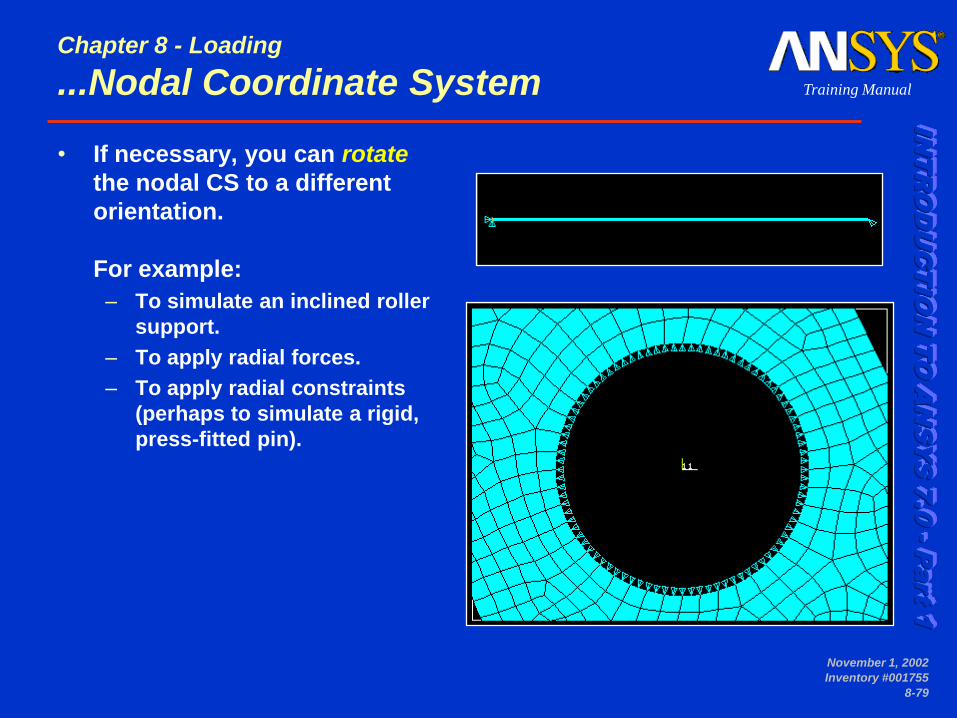
• If necessary, you can rotate

the nodal CS to a different

orientation.

For example:

– To simulate an inclined roller

support.

– To apply radial forces.

– To apply radial constraints

(perhaps to simulate a rigid,

press-fitted pin).

Chapter 8 - Loading

...Nodal Coordinate System

IN

TR

OD

UC

TIO

N T

O A

NS

YS

7

.0

- P

art 1

Training Manual

November 1, 2002

Inventory #001755

8-80

• To “rotate nodes,” use this four-step procedure:

1. Select the desired nodes.

2. Activate the coordinate system (or create a local CS)

into which you want to rotate the nodes, e.g, CSYS,1.

3. Choose Main Menu > Preprocessor > Modeling >

Move/Modify > Rotate Node CS > To Active CS, then press

[Pick All] in the picker.

Or issue NROTAT,ALL.

4. Reactivate all nodes.

• Note: When you apply symmetry on anti-symmetry

boundary conditions, ANSYS automatically rotates all

nodes on that boundary.

Chapter 8 - Loading

...Nodal Coordinate System

IN

TR

OD

UC

TIO

N T

O A

NS

YS

7

.0

- P

art 1

Training Manual

November 1, 2002

Inventory #001755

8-81

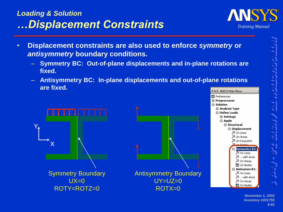
• Displacement constraints are also used to enforce symmetry or

antisymmetry boundary conditions.

– Symmetry BC: Out-of-plane displacements and in-plane rotations are

fixed.

– Antisymmetry BC: In-plane displacements and out-of-plane rotations

are fixed.

Antisymmetry Boundary

UY=UZ=0

ROTX=0

Symmetry Boundary

UX=0

ROTY=ROTZ=0

Y

X

Loading & Solution

…Displacement Constraints

IN

TR

OD

UC

TIO

N T

O A

NS

YS

7

.0

- P

art 1

Training Manual

November 1, 2002

Inventory #001755

8-82

• A force is a concentrated load (or “point

load”) that you can apply at a node or

keypoint.

• Point loads such as forces are

appropriate for line element models

such as beams, spars, and springs.

In solid and shell models, point loads

usually cause a stress singularity, but

are acceptable if you ignore stresses in

the vicinity. Remember, you can use

select logic to “ignore” the elements in

the vicinity of the point load.

Loading & Solution

Concentrated Forces

IN

TR

OD

UC

TIO

N T

O A

NS

YS

7

.0

- P

art 1

Training Manual

November 1, 2002

Inventory #001755

8-83

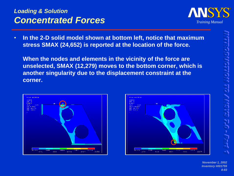
• In the 2-D solid model shown at bottom left, notice that maximum

stress SMAX (24,652) is reported at the location of the force.

When the nodes and elements in the vicinity of the force are

unselected, SMAX (12,279) moves to the bottom corner, which is

another singularity due to the displacement constraint at the

corner.

Loading & Solution

Concentrated Forces

IN

TR

OD

UC

TIO

N T

O A

NS

YS

7

.0

- P

art 1

Training Manual

November 1, 2002

Inventory #001755

8-84

By unselecting nodes and elements near the bottom corner, you

get the expected stress distribution with SMAX (7,895) near the

top hole.

Loading & Solution

…Concentrated Forces

IN

TR

OD

UC

TIO

N T

O A

NS

YS

7

.0

- P

art 1

Training Manual

November 1, 2002

Inventory #001755

8-85

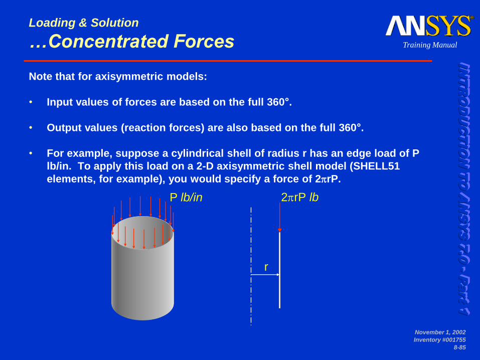
Note that for axisymmetric models:

• Input values of forces are based on the full 360°.

• Output values (reaction forces) are also based on the full 360°.

• For example, suppose a cylindrical shell of radius r has an edge load of P

lb/in. To apply this load on a 2-D axisymmetric shell model (SHELL51

elements, for example), you would specify a force of 2prP.

r

P lb/in 2prP lb

Loading & Solution

…Concentrated Forces

IN

TR

OD

UC

TIO

N T

O A

NS

YS

7

.0

- P

art 1

Training Manual

November 1, 2002

Inventory #001755

8-86

Verifying applied loads

• Plot them by activating load symbols:

– Utility Menu > PlotCtrls > Symbols

– Commands -- /PBC, /PSF, /PBF

• Or list them:

– Utility Menu > List > Loads >

Loading & Solution

Verifying Loads

Structural Analysis

Chapter 10

IN

TR

OD

UC

TIO

N T

O A

NS

YS

7

.0

- P

art 1

Training Manual

November 1, 2002

Inventory #001755

10-88

• Element type

• The table below shows commonly used structural element types.

• The nodal DOF’s may include: UX, UY, UZ, ROTX, ROTY, and ROTZ.

2-D Solid 3-D Solid 3-D Shell Line Elements

Linear PLANE42 SOLID45 SOLID185

SHELL63 SHELL181

BEAM3

BEAM4

BEAM188

Quadratic PLANE82 PLANE2

SOLID95 SOLID92 SOLID186

SHELL93 BEAM189

Commonly used structural element types

Chapter 10 – A. Preprocessing

Meshing

• Material properties

– Minimum requirement is Young’s Modulus, EX. If Poisson’s Ratio is

not entered a default of 0.3 will be assumed.

– Setting preferences to “Structural” limits the Material Model GUI to

display only structural properties.

• Real constants and Section properties

– Primarily needed for shell and line elements.

IN

TR

OD

UC

TIO

N T

O A

NS

YS

7

.0

- P

art 1

Training Manual

November 1, 2002

Inventory #001755

10-89

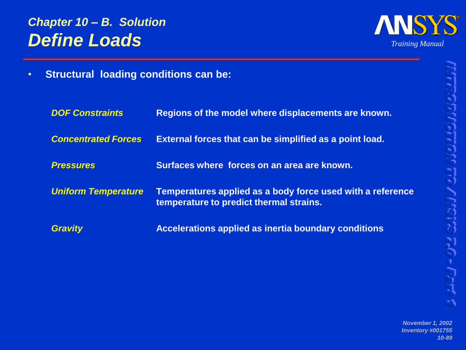
• Structural loading conditions can be:

DOF Constraints Regions of the model where displacements are known.

Concentrated Forces External forces that can be simplified as a point load.

Pressures Surfaces where forces on an area are known.

Uniform Temperature Temperatures applied as a body force used with a reference

temperature to predict thermal strains.

Gravity Accelerations applied as inertia boundary conditions

Chapter 10 – B. Solution

Define Loads

IN

TR

OD

UC

TIO

N T

O A

NS

YS

7

.0

- P

art 1

Training Manual

November 1, 2002

Inventory #001755

10-90

Displacement Constraints

• Used to specify where the model is fixed (zero displacement locations).

• Can also be non-zero, to simulate a known deflection.

• To apply displacement constraints :

– Main Menu > Solution > Define Loads > Apply > Structural > Displacement

• Choose where you want to apply the constraint.

• Pick the desired entities in the graphics window.

• Then choose the constraint direction. Value defaults to zero.

– Or use the D family of commands: DK, DL, DA, D.

• Question: In which coordinate system are UX, UY, and UZ interpreted?


Displacement Constraints

IN

TR

OD

UC

TIO

N T

O A

NS

YS

7

.0

- P

art 1

Training Manual

November 1, 2002

Inventory #001755

10-91

• To apply a force, the following information is needed:

– node or keypoint number (which you can identify by picking)

– force magnitude (which should be consistent with the system of units

you are using)

– direction of the force — FX, FY, or FZ

Use:

– Main Menu > Solution > Define Loads > Apply > Structural > Force/Moment

– Or the commands FK or F

• Question: In which coordinate system are FX, FY, and FZ

interpreted?


Concentrated Forces

IN

TR

OD

UC

TIO

N T

O A

NS

YS

7

.0

- P

art 1

Training Manual

November 1, 2002

Inventory #001755

10-92

Pressures

• To apply a pressure:

– Main Menu > Solution > Define Loads > Apply

Structural > Pressure

• Choose where you want to apply the

pressure -- usually on lines for 2-D

models, on areas for 3-D models.

• Pick the desired entities in the graphics

window.

• Then enter the pressure value.

A positive value indicates a

compressive pressure (acting towards

the centroid of the element).

– Or use the SF family of commands: SFL,

SFA, SFE, SF.


Pressure

IN

TR

OD

UC

TIO

N T

O A

NS

YS

7

.0

- P

art 1

Training Manual

November 1, 2002

Inventory #001755

10-93

• For a 2-D model, where pressures

are usually applied on a line, you

can specify a tapered pressure

by entering a value for both the I

and J ends of the line.

• I and J are determined by the line

direction. If you see the taper

going in the wrong direction,

simply reapply the pressure with

the values reversed.

VALI = 500

500

L3

500

VALI = 500

VALJ = 1000

L3

1000

500

VALI = 1000

VALJ = 500

L3

1000 500


…Pressure

IN

TR

OD

UC

TIO

N T

O A

NS

YS

7

.0

- P

art 1

Training Manual

November 1, 2002

Inventory #001755

10-94

Uniform Temperature

• To uniform temperature

– Main Menu > Solution > Define Loads > Apply >

Structural > Temperature > Uniform Temp

– Or use the TUNIF command.


Uniform temperature

• To define reference temperature

– Main Menu > Solution > Load Step Opts > Other > Reference Temp

– Or use the TREF command or as MP,REFT

LTT refth )( • Recall,

IN

TR

OD

UC

TIO

N T

O A

NS

YS

7

.0

- P

art 1

Training Manual

November 1, 2002

Inventory #001755

10-95

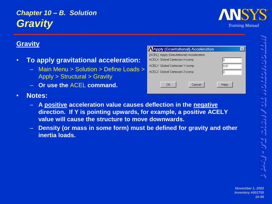
Gravity

• To apply gravitational acceleration:

– Main Menu > Solution > Define Loads >

Apply > Structural > Gravity

– Or use the ACEL command.

• Notes:

– A positive acceleration value causes deflection in the negative

direction. If Y is pointing upwards, for example, a positive ACELY

value will cause the structure to move downwards.

– Density (or mass in some form) must be defined for gravity and other

inertia loads.


Gravity

IN

TR

OD

UC

TIO

N T

O A

NS

YS

7

.0

- P

art 1

Training Manual

November 1, 2002

Inventory #001755

10-96

Modifying and Deleting Loads

• To modify a load value, simply reapply the load

with the new value.

• To delete loads:

– Main Menu > Solution > Define Loads > Delete

– When you delete solid model loads, ANSYS also

automatically deletes all corresponding finite element

loads.


Modifying and Deleting Loads

IN

TR

OD

UC

TIO

N T

O A

NS

YS

7

.0

- P

art 1

Training Manual

November 1, 2002

Inventory #001755

10-97

Static vs. Dynamic Analysis

• A static analysis assumes that only the stiffness forces are

significant.

• A dynamic analysis takes into account all three types of forces.

• For example, consider the analysis of a diving board.

– If the diver is standing still, it might be sufficient to do

a static analysis.

– But if the diver is jumping up and down, you will need

to do a dynamic analysis.


Solutions Options

IN

TR

OD

UC

TIO

N T

O A

NS

YS

7

.0

- P

art 1

Training Manual

November 1, 2002

Inventory #001755

10-98

• Inertia and damping forces are usually significant if the applied

loads vary rapidly with time.

• Therefore you can use time-dependency of loads as a way to

choose between static and dynamic analysis.

– If the loading is constant over a relatively long period of time, choose

a static analysis.

– Otherwise, choose a dynamic analysis.

• In general, if the excitation frequency is less than 1/3 of the

structure’s lowest natural frequency, a static analysis may be

acceptable.


Solutions Options

IN

TR

OD

UC

TIO

N T

O A

NS

YS

7

.0

- P

art 1

Training Manual

November 1, 2002

Inventory #001755

10-99

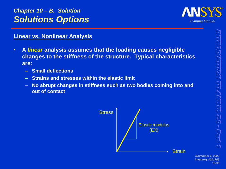
Linear vs. Nonlinear Analysis

• A linear analysis assumes that the loading causes negligible

changes to the stiffness of the structure. Typical characteristics

are:

– Small deflections

– Strains and stresses within the elastic limit

– No abrupt changes in stiffness such as two bodies coming into and

out of contact

Strain

Stress

Elastic modulus

(EX)


Solutions Options

IN

TR

OD

UC

TIO

N T

O A

NS

YS

7

.0

- P

art 1

Training Manual

November 1, 2002

Inventory #001755

10-100

• A nonlinear analysis is needed if the loading causes significant

changes in the structure’s stiffness. Typical reasons for stiffness

to change significantly are:

– Strains beyond the elastic limit (plasticity)

– Large deflections, such as with a loaded fishing rod

– Contact between two bodies

Strain

Stress


Solutions Options

IN

TR

OD

UC

TIO

N T

O A

NS

YS

7

.0

- P

art 1

Training Manual

November 1, 2002

Inventory #001755

10-101

• Reviewing results of a stress analysis generally involves:

– Deformed shape

– Stresses

– Reaction forces

Deformed Shape

• Gives a quick indication of whether the loads were applied in the

correct direction.

• Legend column shows the maximum displacement, DMX.

• You can also animate the deformation.

Chapter 10 – C. Postprocessing

Review Results

IN

TR

OD

UC

TIO

N T

O A

NS

YS

7

.0

- P

art 1

Training Manual

November 1, 2002

Inventory #001755

10-102

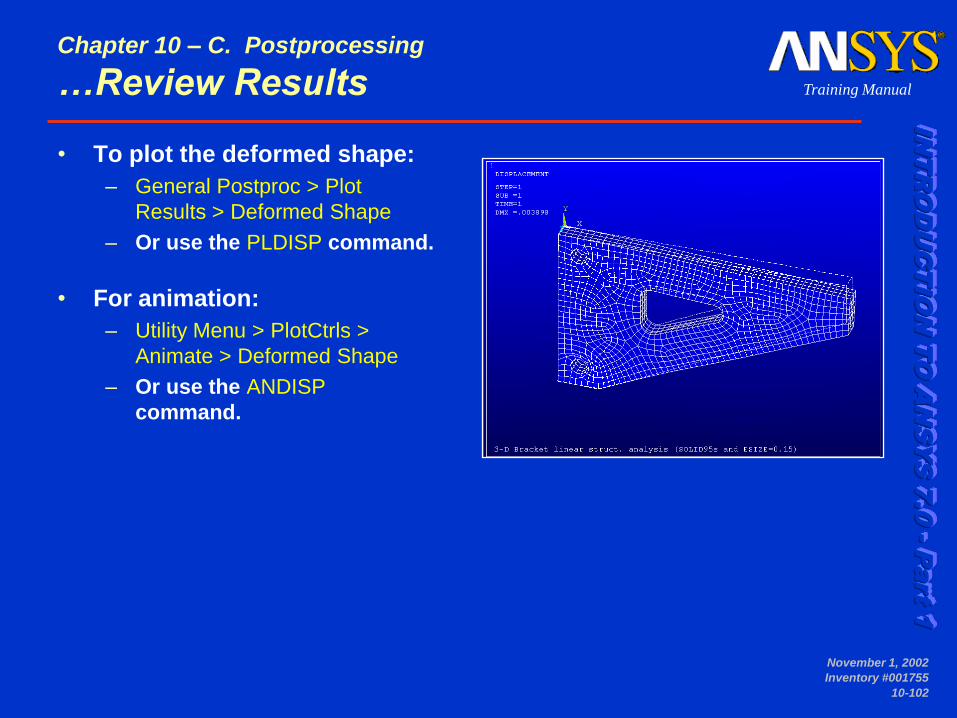
• To plot the deformed shape:

– General Postproc > Plot

Results > Deformed Shape

– Or use the PLDISP command.

• For animation:

– Utility Menu > PlotCtrls >

Animate > Deformed Shape

– Or use the ANDISP

command.


…Review Results

IN

TR

OD

UC

TIO

N T

O A

NS

YS

7

.0

- P

art 1

Training Manual

November 1, 2002

Inventory #001755

10-103

Stresses

• The following stresses are typically available for a 3-D solid

model:

– Component stresses — SX, SY, SZ, SXY, SYZ, SXZ (global Cartesian

directions by default)

– Principal stresses — S1, S2, S3, SEQV (von Mises), SINT (stress

intensity)

• Best viewed as contour plots, which allow you to quickly locate

“hot spots” or trouble regions.

– Nodal solution: Stresses are averaged at the nodes, showing smooth,

continuous contours.

– Element solution: No averaging, resulting in discontinuous contours.


…Review Results

IN

TR

OD

UC

TIO

N T

O A

NS

YS

7

.0

- P

art 1

Training Manual

November 1, 2002

Inventory #001755

10-104

• To plot stress contours:

– General Postproc > Plot Results > Contour Plot > Nodal Solu or PLNSOL command

– General Postproc > Plot Results > Contour Plot > Element Solu or PLESOL command

• You can also animate stress contours:

– Utility Menu > PlotCtrls > Animate > Deformed Results... or ANCNTR command


…Review Results

Postprocessing

Chapter 13

IN

TR

OD

UC

TIO

N T

O A

NS

YS

7

.0

- P

art 1

Training Manual

November 1, 2002

Inventory #001755

13-106

• There are many ways to review results in the general

postprocessor (POST1), some of which have already been

covered.

• In this chapter, we will explore two additional methods — query

picking and path operations — and also introduce you to the

concepts of results transformation, error estimation, and load

case combination.

Chapter 13 - Postprocessing

Overview

IN

TR

OD

UC

TIO

N T

O A

NS

YS

7

.0

- P

art 1

Training Manual

November 1, 2002

Inventory #001755

13-107

• Query picking allows you to “probe” the model for stresses,

displacements, or other results quantities at any picked location.

• You can also quickly locate the maximum and minimum values of

the item being queried.

• Available only through the GUI (no commands):

– General Postproc > Query Results > Nodal or Element or Subgrid Solu

– Choose a results quantity and press OK

PowerGraphics

OFF

PowerGraphics

ON


Query Picking

IN

TR

OD

UC

TIO

N T

O A

NS

YS

7

.0

- P

art 1

Training Manual

November 1, 2002

Inventory #001755

13-108

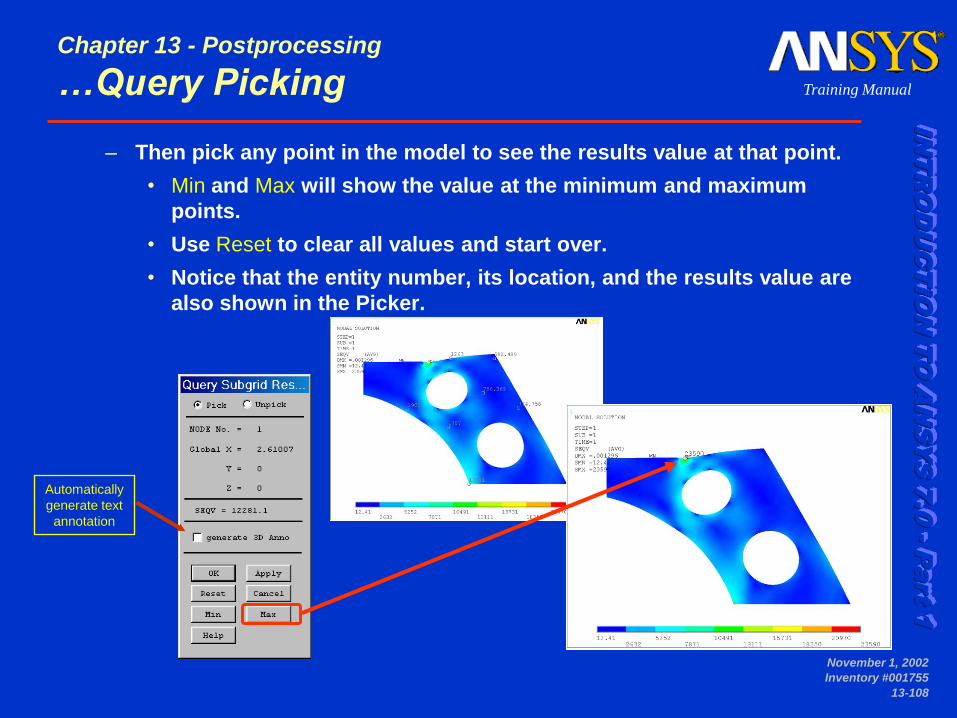
– Then pick any point in the model to see the results value at that point.

• Min and Max will show the value at the minimum and maximum

points.

• Use Reset to clear all values and start over.

• Notice that the entity number, its location, and the results value are

also shown in the Picker.

Automatically

generate text

annotation


…Query Picking

IN

TR

OD

UC

TIO

N T

O A

NS

YS

7

.0

- P

art 1

Training Manual

November 1, 2002

Inventory #001755

13-109

• Demo: – Continue from the last multi-load-step solution of rib.db

– Plot SEQV for load step 1

– Query “Nodal Solu” SEQV at several locations, including MIN & MAX. (Switch to

full graphics if needed.)

– Switch to PowerGraphics and query “Subgrid Solu.”


…Query Picking

IN

TR

OD

UC

TIO

N T

O A

NS

YS

7

.0

- P

art 1

Training Manual

November 1, 2002

Inventory #001755

13-110

• All direction-dependent quantities that you view in POST1, such

as component stresses, displacements, and reaction forces, are

reported in the results coordinate system (RSYS).

• RSYS defaults to 0 (global Cartesian). That is, POST1 transforms

all results to global Cartesian by default, including results at

“rotated” nodes.

• But there are many situations — such as pressure vessels and

spherical structures — where you need to check the results in a

cylindrical, spherical, or other local coordinate system.


Results Coordinate System

IN

TR

OD

UC

TIO

N T

O A

NS

YS

7

.0

- P

art 1

Training Manual

November 1, 2002

Inventory #001755

13-111

• To change the results CS to a different

system, use:

– General Postproc > Options for Outp…

– or the RSYS command

All subsequent contour plots, listings, query picks, etc. will report

the values in that system.

Default orientation

RSYS,0

Local cylindrical

system RSYS,11

Global cylindrical

system RSYS,1


…Results Coordinate System

IN

TR

OD

UC

TIO

N T

O A

NS

YS

7

.0

- P

art 1

Training Manual

November 1, 2002

Inventory #001755

13-112

• RSYS,SOLU

– Sets the results CS to “As calculated.”

– All subsequent contour plots, listings, query picks, etc. will report the

values in the nodal and element coordinate systems.

• DOF results and reaction forces will be in the nodal CS.

• Stresses, strains, etc. will be in the element CS. (The orientation of

the element CS depends on the element type and the ESYS

attribute of the element. Most solid elements, for example, default

to global Cartesian.)

– Not supported by PowerGraphics.


…Results Coordinate System

IN

TR

OD

UC

TIO

N T

O A

NS

YS

7

.0

- P

art 1

Training Manual

November 1, 2002

Inventory #001755

13-113

• Another way to review results is via path operations, which allow

you to:

– map results data onto an arbitrary “path” through the model

– perform mathematical operations along the path, including integration

and differentiation

– display a “path plot” — see how a result item varies along the path

• Available only for models containing 2-D or 3-D solid elements or

shell elements.


Path Operations

IN

TR

OD

UC

TIO

N T

O A

NS

YS

7

.0

- P

art 1

Training Manual

November 1, 2002

Inventory #001755

13-114

• Three steps to produce a path plot:

– Define a path

– Map data onto the path

– Plot the data

1. Define a Path

– Requires the following information:

• Points defining the path (2 to 1000). You can use existing nodes or

locations on the working plane.

• Path curvature, determined by the active coordinate system

(CSYS).

• A name for the path.


…Path Operations

IN

TR

OD

UC

TIO

N T

O A

NS

YS

7

.0

- P

art 1

Training Manual

November 1, 2002

Inventory #001755

13-115

1. Define a Path (cont’d)

– First activate the desired coordinate system (CSYS).

– General Postproc > Path Operations > Define Path > By Nodes or On

Working Plane

• Pick the nodes or WP locations that form the desired path, and

press OK

• Choose a path name. The nSets and nDiv fields are best left to

default in most cases.


…Path Operations

From

To

IN

TR

OD

UC

TIO

N T

O A

NS

YS

7

.0

- P

art 1

Training Manual

November 1, 2002

Inventory #001755

13-116

2. Map Data onto Path

– General Postproc > Path Operations > Map onto Path (or PDEF

command)

• Choose desired quantity, such as SEQV.

• Enter a label for the quantity, to be used on plots and listings.

– You can now display the path if needed.

• General Postproc > Path Operations > Plot Paths

• (or issue /PBC,PATH,1 followed by NPLOT or EPLOT)


…Path Operations

IN

TR

OD

UC

TIO

N T

O A

NS

YS

7

.0

- P

art 1

Training Manual

November 1, 2002

Inventory #001755

13-117

3. Plot the Data

– You can plot path items either on a graph:

• PLPATH or General Postproc > Path Operations > Plot Path Item >

On Graph

– or along path geometry:

• PLPAGM or General Postproc > Path Operations > Plot Path Item >

On Geometry


…Path Operations

IN

TR

OD

UC

TIO

N T

O A

NS

YS

7

.0

- P

art 1

Training Manual

November 1, 2002

Inventory #001755

13-118

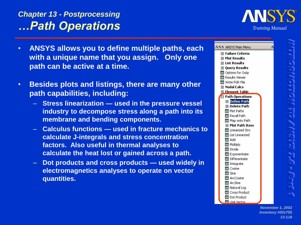
• ANSYS allows you to define multiple paths, each

with a unique name that you assign. Only one

path can be active at a time.

• Besides plots and listings, there are many other

path capabilities, including:

– Stress linearization — used in the pressure vessel

industry to decompose stress along a path into its

membrane and bending components.

– Calculus functions — used in fracture mechanics to

calculate J-integrals and stress concentration

factors. Also useful in thermal analyses to

calculate the heat lost or gained across a path.

– Dot products and cross products — used widely in

electromagnetics analyses to operate on vector

quantities.


…Path Operations

IN

TR

OD

UC

TIO

N T

O A

NS

YS

7

.0

- P

art 1

Training Manual

November 1, 2002

Inventory #001755

13-119

• Demo: – Continue with rib postprocessing…

– Plot nodes, then switch to CSYS,1 if desired

– Define a path using nodes

– Map SX or SEQV or other data onto path

– Plot the path itself

– Plot the path item on graph and on geometry

– Define a second path elsewhere in the model and show how to toggle between

the two.


…Path Operations

IN

TR

OD

UC

TIO

N T

O A

NS

YS

7

.0

- P

art 1

Training Manual

November 1, 2002

Inventory #001755

13-120

• The finite element solution calculates stresses on a per-element

basis, i.e, stresses are individually calculated in each element.

• When you plot nodal stress contours in POST1, however, you will

see smooth contours because the stresses are averaged at the

nodes.

If you plot the element solution, you will see unaveraged data,

which shows the discontinuity between elements.

Elem 1 Elem 2

savg = 1100

s = 1200 s = 1000

savg = 1200

s = 1300 s = 1100

• The difference between averaged and

unaveraged stresses gives an indication

of how “good” or how “bad” the mesh is.

This is the basis for error estimation.

Chapter 13 – Postprocessing

Error Estimation

IN

TR

OD

UC

TIO

N T

O A

NS

YS

7

.0

- P

art 1

Training Manual

November 1, 2002

Inventory #001755

13-121

• Error estimation is available only in POST1 and is valid only for:

– linear static structural and linear steady-state thermal analyses

– solid elements (2-D and 3-D) and shell elements

– Full Graphics (not PowerGraphics)

If these conditions are not met, ANSYS automatically turns off

error estimation calculations.

• To manually activate or deactivate error estimation, use

– ERNORM,ON/OFF

– or General Postproc > Options for Outp


…Error Estimation

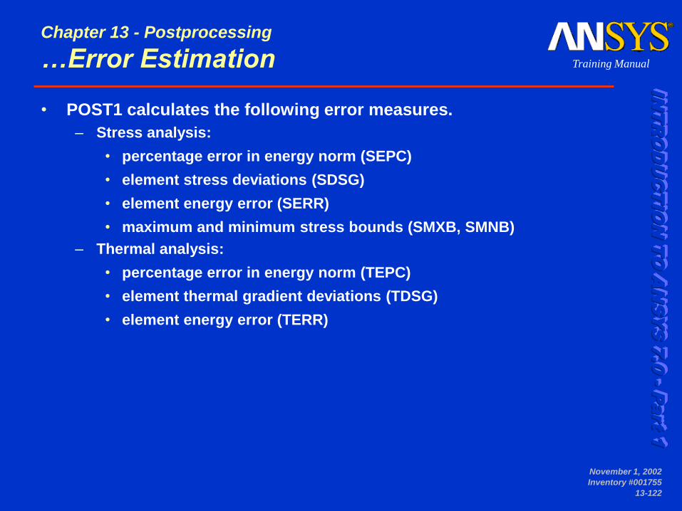
IN

TR

OD

UC

TIO

N T

O A

NS

YS

7

.0

- P

art 1

Training Manual

November 1, 2002

Inventory #001755

13-122

• POST1 calculates the following error measures.

– Stress analysis:

• percentage error in energy norm (SEPC)

• element stress deviations (SDSG)

• element energy error (SERR)

• maximum and minimum stress bounds (SMXB, SMNB)

– Thermal analysis:

• percentage error in energy norm (TEPC)

• element thermal gradient deviations (TDSG)

• element energy error (TERR)


…Error Estimation

IN

TR

OD

UC

TIO

N T

O A

NS

YS

7

.0

- P

art 1

Training Manual

November 1, 2002

Inventory #001755

13-123

Percentage error in energy norm (SEPC)

• SEPC is a rough estimate of the stress error (or displacement,

temperature, or thermal flux) over the entire set of selected

elements.

• Can be used to compare similar models of similar structures

subjected to similar loadings.

• SEPC is shown in the legend column of deformed shape displays.

You can list it manually using PRERR or General Postproc > List

Results > Percent Error.


…Error Estimation

IN

TR

OD

UC

TIO

N T

O A

NS

YS

7

.0

- P

art 1

Training Manual

November 1, 2002

Inventory #001755

13-124

• As a general rule of thumb,

look for SEPC to be 10% or

less. If it is higher, then:

– Check for point loads or

other stress singularities and

unselect elements in the

vicinity.

– If it is still higher, plot the

element energy error. The

elements with high values of

energy error are candidates

for mesh refinement.

SEPC = 35.149

SEPC = 3.484


…Error Estimation

IN

TR

OD

UC

TIO

N T

O A

NS

YS

7

.0

- P

art 1

Training Manual

November 1, 2002

Inventory #001755

13-125

Element stress deviations (SDSG)

• SDSG is a measure of the amount by

which an element’s stress disagrees with

the stress averages at its nodes.

• You can plot SDSG contours using

PLESOL,SDSG or General Postproc > Plot

Results > Contour Plot > Element Solu...

• A high value of SDSG is not necessarily

bad, especially if it is a small percentage

of the nominal stresses in the structure.

For example, this plate-with-a-hole model

shows only a 1.5% stress deviation in the

region of interest.

SDSG at location of interest

= ~450 psi, which is ~1.5% of

~30,000 psi nominal stress


…Error Estimation

IN

TR

OD

UC

TIO

N T

O A

NS

YS

7

.0

- P

art 1

Training Manual

November 1, 2002

Inventory #001755

13-126

Element energy error (SERR)

• SERR is the energy associated with the stress mismatches at the

nodes of the element. This is the basic error measure from which

the other error quantities are derived. SERR has units of energy.

• To plot SERR contours, issue PLESOL,SERR or General Postproc >

Plot Results > Contour Plot > Element Solu

• Generally, the elements with the highest SERR are candidates for

mesh refinement. However, since SERR will always be highest at

stress singularities, be sure to unselect those elements first.


…Error Estimation

IN

TR

OD

UC

TIO

N T

O A

NS

YS

7

.0

- P

art 1

Training Manual

November 1, 2002

Inventory #001755

13-127

Stress bounds (SMXB and SMNB)

• The stress bounds can help you determine the potential effect of

mesh discretization error on the maximum stress.

• They are displayed on stress contour plots in the legend column

as SMXB (upper bound) and SMNB (lower bound).

• The bounds are not estimates of the actual maximum and

minimum, but they do define a “confidence band.” Without other

supporting verification, you have no basis for believing that the

true maximum stress is below SMXB.


…Error Estimation

IN

TR

OD

UC

TIO

N T

O A

NS

YS

7

.0

- P

art 1

Training Manual

November 1, 2002

Inventory #001755

13-128

• Caution: If you don’t unselect elements near stress singularities,

the stress bounds are meaningless, as shown below.

SMXB = 6,401 SMXB = 15,750


…Error Estimation

IN

TR

OD

UC

TIO

N T

O A

NS

YS

7

.0

- P

art 1

Training Manual

November 1, 2002

Inventory #001755

13-129

• Whenever you solve multiple load steps, the results of each load

step are stored as separate sets on the results file (identified by load

step number).

• A load case combination is an operation between two sets of

results, which are called load cases.

– The operation occurs between one load case in the database and the

second load case on the results file.

– The result of the operation — the combined load case — is stored back

in the database.

Load case in database

(computer memory)

Load case

on results file Combined load case in database

overwrites previous contents


Load Case Combinations

IN

TR

OD

UC

TIO

N T

O A

NS

YS

7

.0

- P

art 1

Training Manual

November 1, 2002

Inventory #001755

13-130

Typical procedure:

1. Create the load cases

2. Read one load case into the database

3. Perform the desired operation


…Load Case Combinations

IN

TR

OD

UC

TIO

N T

O A

NS

YS

7

.0

- P

art 1

Training Manual

November 1, 2002

Inventory #001755

13-131

Create Load Cases

• A load case simply acts as a pointer to a set

of results. It requires two pieces of

information:

– a unique ID number

– the results set it represents (load step and

substep number)

• Use the LCDEF command or General

Postproc > Load Case > Create Load Case



IN

TR

OD

UC

TIO

N T

O A

NS

YS

7

.0

- P

art 1

Training Manual

November 1, 2002

Inventory #001755

13-132

Read One Load Case into the Database (memory)

• Simply identify the results set by its load case

number using LCASE or General Postproc > Load

Case > Read Load Case.

• Or use one of the standard “Read Results” choices

in the postprocessor (SET command).



IN

TR

OD

UC

TIO

N T

O A

NS

YS

7

.0

- P

art 1

Training Manual

November 1, 2002

Inventory #001755

13-133

Perform the Desired Operation

• Many operations are available as shown in

the menu here.

• Use the LCOPER command or General

Postproc > Load Case > Add, Subtract, etc.

• Remember that the results of the operation

are stored in the database (memory). The

combined load case is identified on plots

and listings as number 9999.



IN

TR

OD

UC

TIO

N T

O A

NS

YS

7

.0

- P

art 1

Training Manual

November 1, 2002

Inventory #001755

13-134

• There are two useful options to

save the combined load case:

– Write a load case file

– Append the load case to the results

file

• Writing a load case file (LCWRITE

or General Postproc > Write Results)

creates a file that is similar to, but

much smaller than the results file.

• The Append option (RAPPND or

General Postproc > Load Case >

Write Load Case) allows you to add

the combined load case to the

results file and identify it with a

given load step number and time

value.



IN

TR

OD

UC

TIO

N T

O A

NS

YS

7

.0

- P

art 1

Training Manual

November 1, 2002

Inventory #001755

13-135

• Refer to your Workshop Supplement for instructions:

W13A. Connecting Rod

W13B. Spherical Shell

W13C. Axisymmetric Fin with Multiple Load Steps


Workshops

workshops/ws13.ppt

workshops/ws12.ppt

workshops/ws13.ppt

workshops/ws12.ppt

workshops/ws13.ppt

IN

TR

OD

UC

TIO

N T

O A

NS

YS

7

.0

- P

art 1

Training Manual

November 1, 2002

Inventory #001755

13-136

• The Results Viewer is a specialized postprocessing menu and graphic

system.

– Fast graphics for large models or models that have many time steps

– Easy to use menu system for quick results viewing


Results Viewer

IN

TR

OD

UC

TIO

N T

O A

NS

YS

7

.0

- P

art 1

Training Manual

November 1, 2002

Inventory #001755

13-137

• Can be created two different ways …

– Use the POUTRES command before solving

to write a jobname.pgr file during solution.

– Main Menu > Solution > Load Step Opts >

Output Cntrls > PGR File

Hold CTRL key for

multiple selection


…Results Viewer

IN

TR

OD

UC

TIO

N T

O A

NS

YS

7

.0

- P

art 1

Training Manual

November 1, 2002

Inventory #001755

13-138

– Use the PGWRITE command after solution

to write a jobname.pgr file.

– General Postproc > Write PGR File


…Results Viewer

IN

TR

OD

UC

TIO

N T

O A

NS

YS

7

.0

- P

art 1

Training Manual

November 1, 2002

Inventory #001755

13-139

• Open the Results Viewer from the General Post Processor.


…Results Viewer

IN

TR

OD

UC

TIO

N T

O A

NS

YS

7

.0

- P

art 1

Training Manual

November 1, 2002

Inventory #001755

13-140

Element Plot

Nodal/element/vector/trace

results plots

Query Results

Animate using

PNG files

List

Results

Image Capture

Results Set

Locator


…Results Viewer

Time History

Variable Viewer

Report Generation

Mode

Report

Image

Capture

Time

Load Step

Substep

Raise

Hidden

Report

Animation

Capture

Report

Listing

Capture

Report

Table

Capture

IN

TR

OD

UC

TIO

N T

O A

NS

YS

7

.0

- P

art 1

Training Manual

November 1, 2002

Inventory #001755

13-141

• The graphics window becomes “Context Sensitive”.

Right Click on Model


…Results Viewer

Context-sensitive graphics window

IN

TR

OD

UC

TIO

N T

O A

NS

YS

7

.0

- P

art 1

Training Manual

November 1, 2002

Inventory #001755

13-142

Right Click on Contour Legend



…Results Viewer

IN

TR

OD

UC

TIO

N T

O A

NS

YS

7

.0

- P

art 1

Training Manual

November 1, 2002

Inventory #001755

13-143


Right Click on Contour Bar


…Results Viewer

IN

TR

OD

UC

TIO

N T

O A

NS

YS

7

.0

- P

art 1

Training Manual

November 1, 2002

Inventory #001755

13-144

Chapter 13 – Postprocessing

Variable Viewer

• The Variable Viewer is a specialized tool allowing one to postprocess results

with respect to time.

• The Variable Viewer can be started by:

– Main Menu > TimeHist Postproc > Variable Viewer

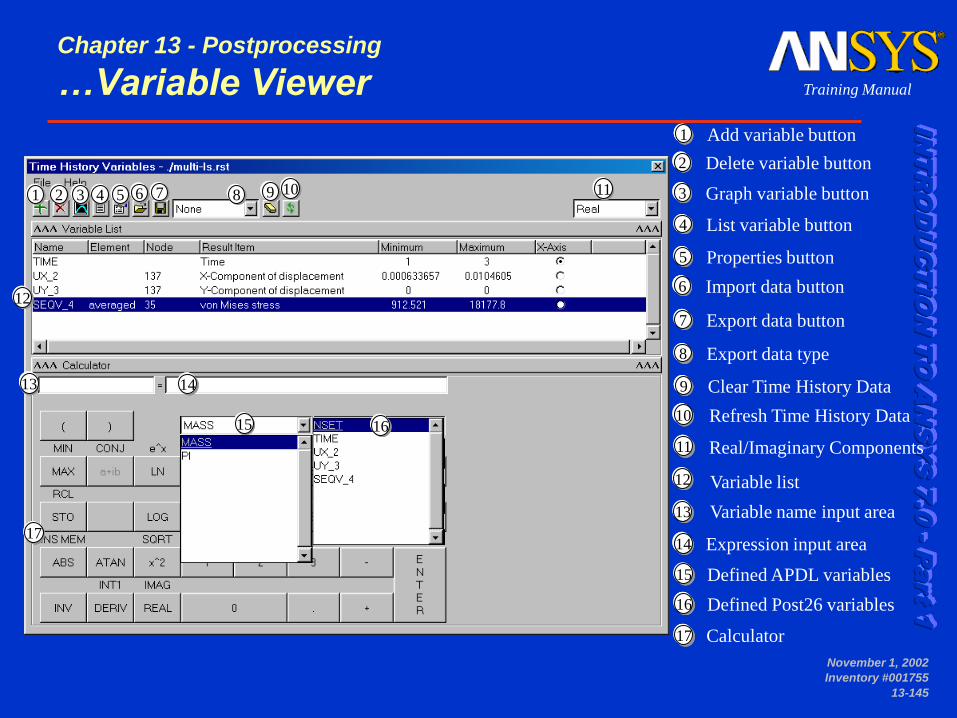
IN

TR

OD

UC

TIO

N T

O A

NS

YS

7

.0

- P

art 1

Training Manual

November 1, 2002

Inventory #001755

13-145

1 2 3 4 5 6 7 8 9 10 11

12

17

Add variable button 1

Delete variable button 2

Graph variable button 3

List variable button 4

Properties button 5

Import data button 6

Export data button 7

Export data type 8

Clear Time History Data 9

Refresh Time History Data 10

Variable name input area

11

Expression input area 14

Defined APDL variables 15

Defined Post26 variables 16

17 Calculator


…Variable Viewer

16

Real/Imaginary Components

Variable list

14

12

13

13

15

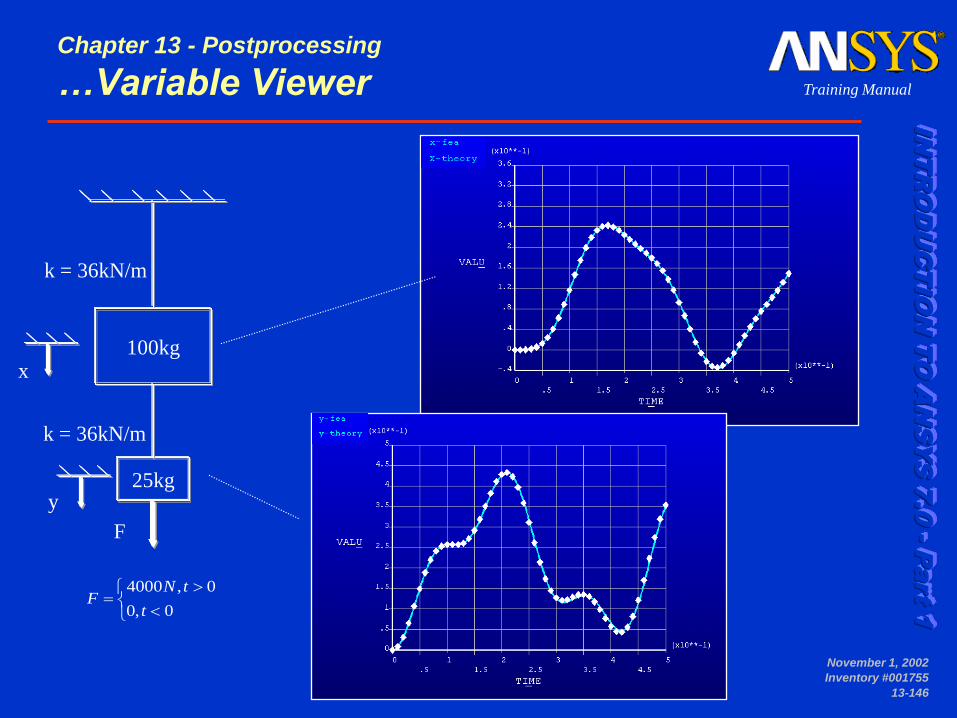
IN

TR

OD

UC

TIO

N T

O A

NS

YS

7

.0

- P

art 1

Training Manual

November 1, 2002

Inventory #001755

13-146

100kg

25kg

k = 36kN/m

F

0,0

0,4000

t

tNF

k = 36kN/m

x

y


…Variable Viewer

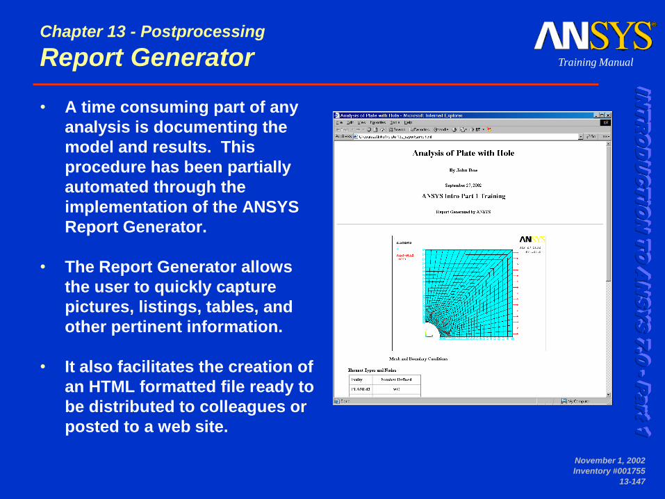
IN

TR

OD

UC

TIO

N T

O A

NS

YS

7

.0

- P

art 1

Training Manual

November 1, 2002

Inventory #001755

13-147

• A time consuming part of any

analysis is documenting the

model and results. This

procedure has been partially

automated through the

implementation of the ANSYS

Report Generator.

• The Report Generator allows

the user to quickly capture

pictures, listings, tables, and

other pertinent information.

• It also facilitates the creation of

an HTML formatted file ready to

be distributed to colleagues or

posted to a web site.


Report Generator

IN

TR

OD

UC

TIO

N T

O A

NS

YS

7

.0

- P

art 1

Training Manual

November 1, 2002

Inventory #001755

13-148

• Launching the Report Generator will

shrink the graphics window and set the

background to white.

• The “Capture Tool” will be opened

allowing the user to grab plots, listings,

and tables. – Utility Menu> File> Report Generator…

or

– ~eui,’euidl::report::toolbar::create’ or

– Select on the Icon Toolbar.

Capture Tool


…Report Generator

IN

TR

OD

UC

TIO

N T

O A

NS

YS

7

.0

- P

art 1

Training Manual

November 1, 2002

Inventory #001755

13-149

Image Capture

(single PNG file)

Animation Capture

(multiple PNG files)

Table

Capture

Settings

HTML Report

Assembler

Listing

Capture

The Log File records

all captures!

• Capture Tool


…Report Generator

IN

TR

OD

UC

TIO

N T

O A

NS

YS

7

.0

- P

art 1

Training Manual

November 1, 2002

Inventory #001755

13-150

HTML Assembler . . .

• A tool that allows quick

organization of ANSYS graphics,

tables, listings .

• Log file can be used as an HTML

template.

– utilize parameter substitution

• The generated HTML file can be

used with Netscape Composer,

Microsoft FrontPage, or any other

HTML editor to finalize the report.


…Report Generator

IN

TR

OD

UC

TIO

N T

O A

NS

YS

7

.0

- P

art 1

Training Manual

November 1, 2002

Inventory #001755

13-151

• Insert TEXT

• Insert any HTML FILE

– possibly created outside ANSYS

• Insert an IMAGE

– possibly one from an external

source like a digital photo

• Insert DYNAMIC DATA

– information specific to your current

ANSYS run like version, run time,

etc.

• Insert a Report Heading

– Including your name, analysis title,

date, and company name


…Report Generator

IN

TR

OD

UC

TIO

N T

O A

NS

YS

7

.0

- P

art 1

Training Manual

November 1, 2002

Inventory #001755

13-152

• Insert information grabbed using

the Capture Tool

• Report Images

– Contour plots, element plots,

volume plots, graphs

• Report Tables

– Material properties, reaction forces,

etc.

• Report Lists

– Stress along a path, constraints,

etc.


…Report Generator

IN

TR

OD

UC

TIO

N T

O A

NS

YS

7

.0

- P

art 1

Training Manual

November 1, 2002

Inventory #001755

13-153

• Preview the report

• Delete sections of the report

• Move sections of the report up or

down


…Report Generator

IN

TR

OD

UC

TIO

N T

O A

NS

YS

7

.0

- P

art 1

Training Manual

November 1, 2002

Inventory #001755

13-154


…Report Generator

2. fea and ansys - dokuz eylül Üniversitesi of... · the open ansys file icon can be used to open...

Documents