2-d symmetry: theory and filter design applications - circuits and

4 IEEE CIRCUITS AND SYSTEMS MAGAZINE 1540-7977/03/$17.00©2003 IEEE THIRD QUARTER 2003

In this comprehensive review article,we present the theory of symmetry intwo-dimensional (2-D) filter functionsand in 2-D Fourier transforms. It isshown that when a filter frequencyresponse possesses symmetry, therealization problem becomes relative-ly simple. Further, when the frequencyresponse has no symmetry, there is atechnique to decompose that fre-quency response into componentseach of which has the desired symme-try. This again reduces the complexityof two-dimensional filter design.A number of filter design examplesare illustrated.

*Paper invited for Circuits andSystems Magazine by Rui J. P. deFigueiredo, chair of the EditorialAdvisory Board.

Hari C. Reddy, I-Hung Khoo, and P. K. Rajan

2-D Symmetry:

Theory and FilterDesign Applications*

Abstract

©D

IGIT

AL

STO

CK

Feature

Introduction

The concept of symmetry is widely applied to geo-metrical figures and has been the subject mattersince the days of Euclid. In fact, symmetry is an

important aspect of nature [1]. During the last few cen-turies, this concept has been applied to abstract entitiessuch as mathematical functions [2] and also in the fields ofquantum mechanics and crystallography. One dimension-al systems and polynomials can only have a limited num-ber of symmetries such as even and odd functionsassociated with, say, filter magnitude and phase functions,respectively. A linear two-dimensional system has a trans-fer function consisting of polynomials in two independentcomplex variables say p1 and p2. In a similar way, three andhigher dimensional system functions can be defined interms of three or more complex variables. These multi-dimensional functions arise from many practical engineer-ing systems. For example, the pictorial signal in videotransmission systems is characterized by its brightnessfunction, which is a function of two spatial variables andthe time variable. Other occurrences of multi-dimensionalsignals that have to be processed or filtered are in theareas of digital imagery for medical x-rays, and in the analy-sis of satellite weather photos; enhancement of televisionpictures from lunar and deep space probes; etc. These two-and higher-dimensional systems may possess many typesof symmetries. During the past twenty years, muchresearch has been done to reduce the complexity of thedesign and implementation of multi-dimensional filters/systems possessing symmetry. Since the impulse (spatio-temporal) response and the two-dimensional frequencyresponse (2-D Fourier transform) are inter-related, it is tobe assumed that the symmetry in one function will inducesome form of symmetry on the other function.

The main aim of this tutorial article is to present theseinterdependencies and also develop conditions on 2-D fil-ter polynomials and functions to possess important sym-metries with application in mind. It will be shown that thecomplexity of the design and implementation could bereduced in 2-D filters, both 2-D infinite impulse response(IIR) as well as 2-D finite impulse response (FIR), by usingvarious types of symmetries in the frequency responsesof these filters [3–14]. It has been established that byusing the constraints arising out of quadrantal, diagonal,four-fold rotational, and octagonal symmetries, efficientfilter design algorithms could be developed [15–20].Some of those design techniques are illustrated in thepaper. In addition, the usefulness of symmetry in reduc-ing the complexity with regard to 2-D Fast Fourier Trans-

form (FFT) algorithm is also presented. The paper is con-cluded with a discussion on symmetrical decompositionof non-symmetric data and transformations. The follow-ing is the layout of the paper section by section.

In “Basic Symmetry Definitions and Understanding”, aunified expression in terms of five parameters is present-ed to represent the various symmetries and a number ofuseful symmetries listed. This is followed in the section“Two-Dimensional Fourier Transform Pairs with Symme-try” by a discussion of symmetry in 2-D Fourier transformpairs. In “Symmetry and 2-D Fast Fourier Transform”, theapplication of symmetry to speed up the fast Fouriertransform calculations for signals with some symmetriesis discussed. The section “Symmetry in 2-D MagnitudeResponse” explores symmetry in the magnitude respons-es of 2-D analog and digital filters and presents designtechniques that effectively utilize the symmetry condi-tions. The application of symmetry conditions developedearlier for the design and implementation of filters whoseresponses do not possess any symmetries is consideredin “Symmetrical Decomposition and Transformation”.The final section concludes the paper with a summary ofthe results presented in this paper.

Basic Symmetry Definitions and Understanding

To follow the symmetry concept, let us consider a realrational function f(x1, x2) in two independent variables x1

and x2. For each pair of values of x1 and x2, the function fassumes a unique value. This can be represented by athree-dimensional object with x1, x2 plane as the basewith height represented by the value of the function ateach point in the plane. This gives a three-dimensionalobject. “A thing is symmetrical if one can subject it to acertain operation and it appears exactly the same afterthe operation” [21]. Expanding on this definition, onemay say that the function f possesses symmetry if a pairof operations, performed simultaneously, one on the vec-tor of variables (constituting (x1, x2)-plane), and the otheron the value or height of the function, leaves the shape ofthe function f undisturbed. The existence of symmetry inf(x1, x2) implies the value of the function at (x1, x2) in aregion is some way related to the value of the function at(x1T , x2T ) where (x1T , x2T ) is obtained by some operationon (x1, x2), this condition being satisfied at all points inthe region. Using this idea, the T − ψ symmetry of a func-tion may be defined as follows [19]:

Definition: A function f(x) is said to possess a T − ψ sym-metry over a domain D if

5THIRD QUARTER 2003 IEEE CIRCUITS AND SYSTEMS MAGAZINE

Hari C. Reddy is with the Department of Electrical Engineering, California State University, Long Beach, California, USA. E-mail:[email protected]. I-Hung Khoo is with the Department of Electrical and Computer Engineering, University of California, Irvine, California,USA. P.K. Rajan is with the Department of Electrical and Computer Engineering, Tennessee Tech University, Cookeville, Tennessee, USA.

ψ[f(T [x]

)] = f(x)

for all x ∈ D (1)

where ψ is an operation on the value of f(x) and T is anoperation on x that maps D onto itself on a one-to-onebasis. Different T − ψ operations give rise to differentsymmetries and the symmetries derive their names, suchas x1 = x2 diagonal reflection anti-symmetry, 4-fold rota-tional conjugate symmetry, and so on, based on the T andψ operations.

In the T − ψ symmetry definition given above, if theregion D consists of all the points in the whole x domain,i.e., D = X, then the function is said to possess aglobal T − ψ symmetry. Here, we will restrict our atten-tion only to global T − ψ symmetries and the adjective“global” will be omitted in their descriptions. We will nextdiscuss the nature of ψ and T operations, and consider afew of the commonly found symmetries.

Nature of ψ -OperationsOf the many possible complex scalar operations, the fol-lowing definition for ψ covers many useful ones:

ψ[f(x)] = |f(x)|ej(δ�f(x)+β t x+φ)(2)

where δ = ±1, �f(x) denotes the argument of f(x), β is a(2 × 1) real constant vector and φ is a real constant. Fromequation (2), it may be seen that ψ does not alter themagnitude of f(x). The three parameters δ, β and φ alteronly the argument of f(x). From this, it is evident that if afunction possesses a T − ψ symmetry with respect to anyset of parameters (δ, β and φ) then the magnitude of thefunction possesses the T − ψ I symmetry, where ψ I rep-resents the identity operation represented by the param-eters δ = 1, β = 0 and φ = 0. Many of the commonlyoccurring symmetries have β = 0. The term β t has beenincluded in the ψ operation to account for some of thedelay type symmetries that may be present in some func-tions. We list in Table 1 four specific ψ -operations used invarious symmetry descriptions along with the commonlyused names and the proposed symbols.

Nature of T-OperationsSimple T -operations that find application in symmetrystudies can be represented by the transformation (knownas affine transformation in geometry):

T[x] = A · x + b (3)

where A is a nonsingular (2 × 2) real square matrix and bis a (2 × 1) real vector.

T is said to be an equiaffine transformation if |A| = ±1in which case corresponding regions in the transformedand the original domains have the same area. T is said tobe a congruent transformation if the Euclidean distancebetween any two points in the original region is equal tothat between the corresponding (image) points in thetransformed region. This will be so if and only if the matrixA is orthogonal, i.e., A = (A−1

)t . It is to be noted that thecompounding of two transformations, T1T2, refers to anoperation T consisting of operation T2 followed by T1. Thecompounding of transformations always obey the asso-ciative law, i.e., T1(T2T3) = (T1T2)T3. In addition, if T1 andT2 are two nonsingular transformations, then T1T2 andT2T1 are also nonsingular transformations.

Some of the well-known T -transformations are: (i) dis-placement transformation; (ii) rotational transformation;and (iii) reflection transformation. In Table 2, we list a fewof the basic transformations involving only reflection androtation.

Here, b = 0 and the A matrices are formed using 1 or−1 as elements on the diagonal or off the diagonal. Thisresults in altogether eight different combinations. One ofthese is the identity operation I, which is a trivial case.The remaining seven operations are shown in Table 2. Ofthese operations, only five are needed as the product ofthese will give the remaining two. As such, in the rest ofthis paper, we will use only the first five operations (i)–(v)listed in Table 2.

It is easy to see that the transformations in Table 2 areequiaffine and congruent. In addition, the following aresome interesting properties:

(a) T1 = −T2 = T7 · T2

(b) T3 = −T4 = T7 · T4

(c) T1 · T2 = T2 · T1 = − I = T7

(d) T3 · T4 = T4 · T3 = − I = T7

(e) T 25 = − I = T7

Further, the T -operations can be clas-sified by the number of cycles. A T -operation is said to be k-cyclic if krepeated T -operations on x yields thesame original x. That is: Tk[x] = x orstated in another way Tk = I (where I

6

δ β φ ψ-operations Symmetry Name Symbol

1 0 0 ψ[f(x)] = f

(x)

Identity symmetry ψI

1 0 π ψ[f(x)] = −f

(x)

Anti-symmetry ψA

−1 0 0 ψ[f(x)] = [

f(x)]∗

Conjugate symmetry ψC

−1 0 π ψ[f(x)] = − [

f(x)]∗

Conjugate anti-symmetry ψCA

Table 1. ψ-operations and the names of the resulting symmetries.

IEEE CIRCUITS AND SYSTEMS MAGAZINE THIRD QUARTER 2003

Type of Symmetry Conditions

Quadrantal Symmetry f(x) = f(T1[x]) = f(T1T2[x]) = f(T2[x])

Diagonal Symmetry f(x) = f(T3[x]) = f(T3T4[x]) = f(T4[x])

Four-Fold (90◦) Rotational Symmetry f(x) = f(T5[x]) = f(T2

5[x]) = f

(T3

5[x])

Octagonal Symmetry f(x) = f(T1[x]) = f(T2[x])= f(T3[x]) = f(T4[x])= f(T5[x]) = f

(T2

5[x]) = f

(T3

5[x])

is the identity matrix). For example, T21 = I and T4

5 = I.So, operations (i)–(iv) listed in Table 2 are 2-cyclic, while(v) is 4-cyclic.

Composite Symmetry Operation andSymmetry ParametersWe now combine the T and ψ operations and define acomposite symmetry operation λ as λ = (T, ψ) =(A, b, δ, β, φ) where T[x] = A · x + b and ψ[f(x)] =|f(x)|ej(δ�f(x)+β t x+φ) .

In terms of λ, the symmetry definition can be given as

λ[f(x)] = f(x), ∀ x ∈ D (4)

The five parameters (A, b, δ, β, φ) describe the symmetryoperation completely and they will hereafter be calledsymmetry parameters and be used to specify the varioussymmetries.

Various T−ψI SymmetriesEmploying the various T and ψ operations, one can gen-erate various symmetries. For example, using the T -oper-ations (i)–(v) in Table 2 and assuming the identity ψ I , wehave the following standard symmetries. (Note that thecorresponding anti-symmetry, conjugate-symmetry, andconjugate-anti-symmetry can be obtained by applying theψA, ψC , and ψCA operations respectively).

(i) Reflection about x1-axis symmetry: f(x) = f(T1[x]).(ii) Reflection about x2-axis symmetry: f(x) = f(T2[x]).(iii) Reflection about x1 = x2 diagonal symmetry:

f(x) = f(T3[x]).(iv) Reflection about x1 = −x2 diagonal symmetry:

f(x) = f(T4[x]).(v) 90◦ clockwise rotational symmetry: f(x) = f(T5[x]).

This also implies f(T5[x]) = f(T25 [x]) and f(T2

5 [x]) =f(T3

5 [x]), through repeated substitution of x = T5[x].

7

A b Name of operation Symbol

(i)

[1 00 −1

]0 Reflection about x1-axis T1

(ii)

[−1 00 1

]0 Reflection about x2-axis T2

(iii)

[0 11 0

]0 Reflection about x1 = x2 diagonal T3

(iv)

[0 −1

−1 0

]0 Reflection about x1 = −x2 diagonal T4

(v)

[0 1

−1 0

]0 90◦ clockwise rotation about origin T5

(vi)

[0 −11 0

]0 90◦ anti-clockwise rotation about origin T6

(vii)

[−1 00 −1

]0 180◦ rotation about origin T7

Table 2. Basic T-operations.

THIRD QUARTER 2003 IEEE CIRCUITS AND SYSTEMS MAGAZINE

Table 3. Definitions of compound T−ψ I symmetries.

(vi) Centro (180◦ rotation) symmetry: f(x) = f(−x). Thiscan also be expressed as f(x) = f(T2

5 [x]) orf(x) = f(T1T2[x]) or f(x) = f(T3T4[x]).

These symmetries are shown in Figures 1 (a)–(f). It isto be noted that the function values in the colored regionsare the same, since we assumed ψ I . For example, in Fig-ure 1(b), the function values in the regions denoted byf(x) and f(T2[x]) are the same. This is clearly the result ofx2-axis reflection symmetry.

The number of cycles in a symmetry determines thenumber of regions in its figure with the same functionvalues. Reflection symmetries about x1-axis, x2-axis,x1 = x2 diagonal, x1 = −x2 diagonal, as well as centrosymmetry, are all 2-cyclic symmetries. So they have tworegions of symmetry in the X -plane. 90◦ clockwise rota-tional symmetry is 4-cyclic. So it has four regions of sym-metry in the X -plane (although only two are shown inFigure 1(e)). For this reason, we usually call it four-fold(90◦) rotational symmetry.

In addition to these basic symmetries, more complexsymmetries can be generated using a combination of dif-

ferent T -operations. For example, using a combination ofT1 and T2 operations, we can obtain quadrantal symme-try. Diagonal symmetry can be obtained using both T3

and T4 operations. These compound symmetries are list-ed in Table 3. (Once again, for illustration, we show onlythe symmetries resulting from the ψ I operation.)

From “Nature of T-Operations,” we can make someimportant observations on the compound symmetries inTable 3:

(a) Quadrantal symmetry is a combination of x1-axisreflection, x2-axis reflection, and centro symmetries. Thepresence of any two of the symmetries implies the exis-tence of the third, i.e. T1 · T2 => − I, − I · T1 => T2, and− I · T2 => T1. So only two of the three symmetries areneeded to ensure quadrantal symmetry. Also, each equa-tion in the quadrantal symmetry condition defines a sym-metry region in the X -plane. Since there are fourequations in the symmetry condition, there will be fourregions of symmetry in the X -plane. Finally, in terms ofcycles, quadrantal symmetry is a double 2-cyclic symme-try (T1 · T2) · (T1 · T2) = I . Because of the cyclical proper-ty, the operation Tm

1 Tn2 , where m and n are integers,

8 IEEE CIRCUITS AND SYSTEMS MAGAZINE THIRD QUARTER 2003

1x

2x

( )f x

[ ]( )4f T x

1 2x x

Diagonal

= −

0

2x

1x( )f x[ ]( )2f T x

0

2x

1x[ ]( )1f T x

( )f x

01x

2x

( )f x

[ ]( )3f T x

1 2x x

Diagonal

=

0

1x

2x

( )f x

( )f x− 01x

2x

( )f x

[ ]( )5f T x

0

Figure 1(b). x2-axis reflection sym-metry.

Figure 1(a). x1-axis reflectionsymmetry.

Figure 1(f). Centro (180◦ rotation)symmetry.

Figure 1(e). −90◦ clockwise rota-tion symmetry.

Figure 1(c). x1 = x2 diagonal reflec-tion symmetry.

Figure 1(d). x1 = −x2 diagonalreflection symmetry.

corresponds to one of the following four possibilities: I,T1T2, T1, or T2.

(b) Diagonal symmetry is a combination of x1 = x2

diagonal, x1 = −x2 diagonal, and centro symmetries. Thepresence of any two of the three symmetries implies theexistence of the third and is enough to ensure diagonalsymmetry. Diagonal symmetry is a double 2-cyclic sym-metry. The operation Tm

3 Tn4 , where m and n are integers,

corresponds to one of the following four possibilities: I,T3T4, T3, or T4. This results in four regions of symmetry inthe X -plane.

(c) Four-fold (90◦) rotational symmetry is a 4-cyclicsymmetry. It is formed by four repeated application of T5.As such, there are four regions of symmetry in the X -plane for 4-fold rotational.

(d) Octagonal symmetry is a combination of quadran-tal, diagonal and 4-fold rotational symmetries. The pres-ence of any two of the three symmetries implies theexistence of the third, and is sufficient to guarantee octag-onal symmetry. More specifically, octagonal symmetrycan result from the presence of 4-fold rotational symmetryand one of the following symmetries: x1-axis reflection, x2-axis reflection, x1 = x2 diagonal reflection, or x1 = −x2

diagonal reflection. So, we can classify octagonal symme-

try as a combination of 4-cyclicand 2-cyclic symmetries. Alterna-tively, octagonal symmetry canalso result from the presence ofany three of the following sym-metries: x1-axis reflection, x2-axisreflection, x1 = x2 diagonalreflection, or x1 = −x2 diagonalreflection. Thus, octagonal sym-metry can also be classified as atriple 2-cyclic symmetry. Finally,since eight equations are in-volved in the symmetry condi-tion, there are eight regions ofsymmetry in the X -plane foroctagonal.

To aid in understanding, Fig-ures 2(a)–(d) show the graphicalinterpretation of the quadrantal,diagonal, rotational, and octago-nal symmetries. Once again, thevalues of the function in the col-ored regions are related to oneanother in the manner specifiedby the ψ operation (i.e. identity,negative, conjugate, or negativeconjugate). From the figures, oneshould be able to confirm, aspreviously discussed, that there

are four regions of symmetry in the X -plane for quadran-tal, diagonal, and 4-fold rotational symmetries, and eightregions for octagonal symmetry. Note that

f(T1T2[x]) = f(T3T4[x]) = f(

T25 [x]

)

= f(−x)

Two-Dimensional Fourier Transform Pairs with Symmetry

Two-dimensional (2-D) Fourier transform plays an impor-tant role in the analysis and design of 2-D linear systems.The transform uniquely relates the impulse or unit sam-ple response of a linear system with its frequencyresponse. Hence, symmetry in one response (eitherimpulse or frequency response) may be expected toinduce some form of symmetry in the other response.The existence of such symmetries can be utilized to sim-plify the analysis and design of these systems. Such uti-lization and the resulting simplification have beenreported in the design and analysis of two and higherdimensional digital filters. Here, we present, in a unifiedmanner, the type of symmetry induced in one function(Fourier transform or inverse Fourier transform) as aresult of a particular symmetry in the other function forboth continuous and discrete-time signals.


1x

2x

( )f x

[ ]( )3f T x

[ ]( )4f T x

[ ]( )3 4f TT x0

Figure 2(b). Diagonal Symmetry.

2x

1x[ ]( )1f T x

( )f x[ ]( )2f T x

[ ]( )1 2f TT x0

1x

2x

( )f x

[ ]( )1f T x

[ ]( )2f T x

[ ]( )3f T x

[ ]( )4f T x

[ ]( )35f T x

[ ]( )25f T x

[ ]( )5f T x

0

Figure 2(d). Octagonal Symmetry.

1x

2x

( )f x

[ ]( )35f T x

[ ]( )25f T x

[ ]( )5f T x

0

Figure 2(c). 4-fold Rotational Symmetry.

Figure 2(a). Quadrantal Symmetry.

Continuous-Time Continuous-Frequency CaseLet g(l) = g(l1, l2), where l1, l2are real numbers, be a two-dimensional signal andG(ω) = G( jω1, jω2) be the two-dimensional Fourier transformof g(l). In general, we assumeg(l) and G(ω) to be complexfunctions of real variables andg(l) is such that its 2-dimension-al Fourier transform G(ω)

exists. If g(l) is the impulseresponse of a stable continuousdomain system, the conditionsfor the existence of its Fouriertransform will always be satis-fied. The Fourier transform pairconnecting g(l) and G(ω) are asfollows:

G(ω) =∫

l∈L

g(l) · e− jωt l · dl (5)

and

g(l) = 1

(2π)2

∫ω∈W

G(ω) · ejltω · dω (6)

where dl �= dl1 · dl2 and dω�= ω1 · dω2.

As g(l) and G(ω) are functions of 2 variables, they maypossess some of the T − ψ symmetries described in thesection “Basic Symmetry Definitions and Understanding.”We next state a theorem which gives the nature of a T − ψ

symmetry that will be present in g(l), given a symmetry inG(ω) and vice-versa. The proof of this theorem can befound in [22].

Theorem 1: Let g(l) and G(ω) form a 2-dimensional Fouri-er transform pair. Then G(ω) possesses a T − ψ symme-try with parameters (A, b, δ, β, φ), |A| = ±1, if and only ifg(l) possesses a T − ψ symmetry with parameters(δ · (A−1

)t, δβ, δ,−δb, btβ + φ) where A, b, δ, β, φ are asdefined in the section “Basic Symmetry Definitions andUnderstanding.”

Observations: Next we make the following observationsbased on Theorem 1.

(i) If (A, b, δ, β, φ)ω and (A, b, δ, β, φ)l are respectivelythe ω-domain and the l-domain symmetry parameters,the corresponding l and ω domain parameters areobtained by the following relations:

(A, b, δ, β, φ)ω ⇒ (δ · (A−1)t, δβ, δ,−δb, btβ + φ)l (7)

and

(A, b, δ, β, φ)l ⇒ (δ · (A−1)t,−δβ, δ, δb, btβ + φ)ω (8)

One can easily verify the compatibility of the two rela-tions by noting that one relation is the inverse of theother relation. The reason for the appearance of the neg-ative sign in front of δb in (7) whereas it is in front of δβ in(8) may be attributed to the differing signs in e± jωt l in thedefinitions of Fourier and inverse Fourier transforms (5)and (6).

(ii) Theorem 1 and the observation (i) also illustratethe duality present in ω and l domain symmetries.

(iii) Further, it may be noted that the nature of sym-metry transformation, such as rotation, reflection, etc., asidentified by the A-matrix remains the same in both the ωand l domains.

(iv) Identical symmetries resu1t in both ω and ldomains if δ = 1, b = 0 and β = 0.

We next illustrate the application of Theorem 1 usingan example.

Example 1: Let G(ω) possess a centro-conjugate symme-try specified by the parameters: (A, b, δ, β, φ)ω =([−1 0

0 −1

],

[00

],−1,

[00

], 0

). Then, as per Theorem 1, the

parameters of the T − ψ symmetry of g(l) will be([1 00 1

],

[00

],−1,

[00

], 0

). Substituting these parameters in the

definition of T − ψ symmetry, we get:


-FFT2

N

[ ]0x

[ ]2x•••

[ ]– 2x

•••

•••

•••

[ ]0 0S

[ ]0 1S

[ ]0 2 –1NS

0NW

–1NW

( )2– 2N

NW –

[ ]0X

[ ]1X

[ ]2 –1NX

[ ]2NX

[ ]2 +1NX

[ ]– 2X

[ ]2X[ ]0 2S

( )2–1N

NW ––1 [ ]– 1X

•••

–1

–1

–1

N

N

N

Figure 3. Symmetry-based FFT Diagram.

∣∣g(l)∣∣ ej{−�g(l)} = g

(l)

i.e.,[g

(l)]∗ = g

(l)

or in other words g(l) possesses an identity conjugatesymmetry. This can only be satisfied if g(l) has real coef-ficients.

Example 2: Let g(l) possess a 4-fold rotational anti-sym-metry specified by the parameters: (A, b, δ, β, φ)l =([

0 −11 0

],

[00

], 1,

[00

], π

). Then, as per Theorem 1, the parame-

ters of the T − ψ symmetry of G(ω) will be([0 −11 0

],

[00

], 1,

[00

], π

). It can be seen that G(ω) possesses

the same 4-fold rotational anti-symmetry, which agreeswith observation (iv).

Example 3: Let a one-dimensional signal g(l) possess atranslation symmetry (periodicity) specified by theparameters: (A, b, δ, β, φ)l = ([1], [L], 1, [0], 0). Then, asper Theorem 1, the parameters of T − ψ symmetryof G(ω) will be ([1], [0], 1, [L], 0). The resulting con-straint on G(ω) is given by

G(ω) · ejLω = G(ω)

It may be noted that this equation will be satisfied only ifG(ω) = 0 for all ω except those discrete frequencies cor-responding to ωk = 2kπ/L. It may be noted that this cor-responds to Fourier transform of periodic signals (i.e.Fourier series).

Continuous-Time Discrete-Frequency Case (Fourier Series)Let h(l) = h(l1, l2) be a 2-D continuous-time periodic sig-nal with periods L1 and L2, respectively in l1 and l2 direc-tions. Let H[k] = H[k1,k2] be the two-dimensionalFourier series coefficients of h(l1, l2). The relationsbetween h(l) and H[k] are given by

H [k] = 1L1 · L2

·L1∫

l1=0

L2∫l2=0

h(l) · e− j·kt ·V·l · dl (9)

and

h(l) =∑

k

H [k] · ej·kt ·V·l (10)

where

V =[

V1 00 V2

]=

[ 2·πL1

0

0 2·πL2

]

represents the fundamental frequencies in the two direc-tions. It may be verified that h(l) is a doubly periodic func-tion indicating the existence of displacement symmetries.In the following, we will consider the general T − ψ sym-metry relations.

Theorem 2: Let H[k] be the Fourier series representationof a periodic function h(l). Then h(l) possesses a T − ψ

symmetry with parameters (A, b, δ, β, φ), |A| = ±1, if andonly if H[k] possesses a T − ψ symmetry with parame-ters (δ · (A−1

)t,−δ · V−1 · β, δ, δ · V · b, btβ + φ) whereA, b, δ, β, φ are as defined in the section “Basic SymmetryDefinitions and Understanding.”

It may be noted that the overall nature of the symme-try parameters in Theorem 1 and 2 are the same except inTheorem 2, the normalizing fundamental frequencymatrix appears. It should also be noted that b and−δ · V−1 · β are integer vectors. The observations made atthe end of the discussions in the continuous domain caseare applicable here also. Consequently, the relationsbetween k and l domain parameters are given by

(A, b, δ, β, φ)l

⇒(δ · (A−1)t,−δ · V−1 · β, δ, δ · V · b, btβ + φ

)k

(11)

and

(A, b, δ, β, φ)k

⇒(δ · (A−1)t, δ · V−1 · β, δ, −δ ·V · b, btβ + φ

)l

(12)


( )1Im z ( )2Im z( )1 Biplanez ,z2

( )1Re z ( )2Re z

θ1 θ20 0

Figure 5. (z1, z2) biplane. (The frequency response is evalu-ated on the unit circles, zi = ejθi .)

1jω

1σ

2jω

2σ

( )1, Biplanes

00

s2

Figure 4. (s1, s2) biplane. (The frequency response is eval-uated on the imaginary axes, si = jωi.)

In the application of this theorem, it should be noted thath(l) is periodic and H[k] is a discrete domain function.

Discrete-Time Continuous-Spectrum CaseLet h(n) = h(n1,n2), where n1, n2 are integers, be a two-dimensional discrete domain signal and H(θ) =H(e− jθ1, e− jθ2) be the two-dimensional Fourier transformof h(n). When h(n) represents the unit sample response ofa discrete domain system, H(θ) will represent its fre-quency response. The Fourier transform pair connectingh(n) and H(θ) are given by:

H(θ) =∑

n∈N2

h(n) · e− jθ tn (13)

and

h(n) = 1(2π)2

∫

θ∈θp

H(θ) · ejntθ · dθ (14)

where θp = {θ | − π ≤ θ1 ≤ π,−π ≤ θ2 ≤ π} and dθ =dθ1 · dθ2.

It may easily be verified from (13) that H(θ) is a peri-odic function of θ with a period of 2π in the θ1 and θ2

directions. As h(n) and H(θ) are functions of two vari-ables, they may possess some of the T − ψ symmetriesdescribed in “Basic Symmetry Definitions and Under-standing.” Because of the periodic nature of H(θ), dis-placement symmetries in θ1 and θ2 directions arealways present. This is due to the discrete nature ofh(n). We will consider the effects of the remaining sym-metries that will be present in h(n), given a symmetry inH(θ) and vice-versa. This is presented in the followingtheorem.

Theorem 3: Let h(n) and H(θ) be a two-dimensional Fouri-er transform pair. Then H(θ) possesses a T − ψ symme-try with parameters (A, b, δ, β, φ), |A| = ±1, if and only ifh(n) possesses a T − ψ symmetry with parameters(δ · (A−1

)t, δβ, δ,−δb, btβ + φ) where A, b, δ, β, φ are asdefined in “Basic Symmetry Definitions and Under-standing.”

The similarity between Theorem 3 and Theorem 1should be obvious. As such, the observations made at theend of the discussion in the continuous domain case areapplicable to the discrete domain case as well. Conse-quently, the relations between θ and n symmetry param-eters are given by:

(A, b, δ, β, φ)θ ⇒ (δ · (A−1)t, δβ, δ,−δb, btβ + φ)n (15)

and

(A, b, δ, β, φ)n ⇒ (δ · (A−1)t,−δβ, δ, δb, btβ + φ)θ (16)

12

Stopband (Gain = 0)

Passband (Gain = 1)

1θ

2θ

π

π

π–

== –

π–

aθ

bθ

aθ bθaθbθ

aθ

bθ

= 2bθ

= 1aθ

0

θ θ2121θ θ

– –

–

–

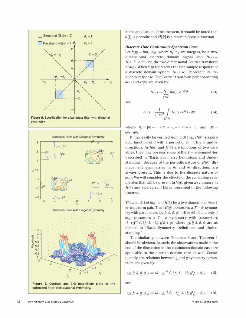
Figure 6. Specification for a bandpass filter with diagonalsymmetry.

– 4– 2

02

4 – 4

– 2

0

2

40

0.20.40.60.81

1.21.4

2

Bandpass Filter With Diagonal Symmetry

1

Mag

nitu

de

θθ

– 3 – 2 – 1 0 1 2 3– 3

– 2

– 1

0

1

2

30.2

0.2

0.2

0.2

0.2

0.2

0.2

0.2

0.2

0.20.2

0.20.4

0.4

0.6

0.6

0.8

0.8

1

1

1

1

1

2

Bandpass Filter With Diagonal Symmetry

θ

θ

Figure 7. Contour and 3-D magnitude plots of the optimized filter with diagonal symmetry.

IEEE CIRCUITS AND SYSTEMS MAGAZINE THIRD QUARTER 2003

In the application of this theorem, it should be notedthat h(n) is a function of discrete domain variable n andh(n) = 0 if n is not an integer vector.

Discrete-Time Discrete-Frequency Case(Discrete Fourier Transform)Let h[n] = h[n1,n2] be a two-dimensional discrete-domain signal defined over 0 ≤ n1 ≤ (N1 − 1) and0 ≤ n2 ≤ (N2 − 1). Then its (N1, N2) length 2-D discreteFourier transform is given by

H [k] = H [k1,k2] =N1−1∑n1=0

N2−1∑n2=0

h [n] · e− j·k t ·V·n,

0 ≤ k1 ≤ (N1 − 1)

0 ≤ k2 ≤ (N2 − 1) (17)

where

V =[ 2·π

N10

0 2·πN2

]

The inverse discrete Fourier transform is given by

h [n] = h [n1,n2]

= 1N1 · N2

·N1−1∑k1=0

N2−1∑k2=0

H [k] · ej·k t ·V·n (18)

It may be noted that even though h[n1,n2] andH[k1,k2] are defined in the square [0, N1 − 1] ×[0, N2 − 1], they satisfy the doubly periodic relationsh [n1 + r1 · N1,n2 + r2 · N2] = h [n1,n2] for any integer r1 and r2 and similarlyH [k1 + r1 · N1,k2 + r2 · N2] = H [k1,k2] for any integer r1

and r2. The symmetry relations between h and H are givenin terms of T − ψ parameters next.

Theorem 4: Let H[k] be the discrete Fourier transform ofh[n]. Then h[n] possesses a T − ψ symmetry withparameters (A, b, δ, β, φ) if and only if H[k] possesses aT − ψ symmetry with parameters(δ · (A−1

)t,−δ · V−1 · β, δ, δ · V · b, btβ + φ) whereA, b, δ, β, φ are as defined in “Basic Symmetry Defini-tions and Understanding.”

As in the previous cases, the symmetry parameters of nand k domains can be written as

(A, b,δ, β, φ)n

⇒ (δ · (A−1)t,−δ · V−1 · β, δ, δ · V · b, btβ + φ)k

(19)and(A, b,δ, β, φ)k

⇒ (δ · (A−1)t, δ · V−1 · β, δ,−δ · V · b, btβ + φ)n

(20)


Stopband (Gain = 0)Passband (Gain = 1)

1θ

2θ

π

( )

π–

( )( )

( ), 0.5–

π– π0

π π

π π–

, 0.5π π

π π0.5–,0.5–,

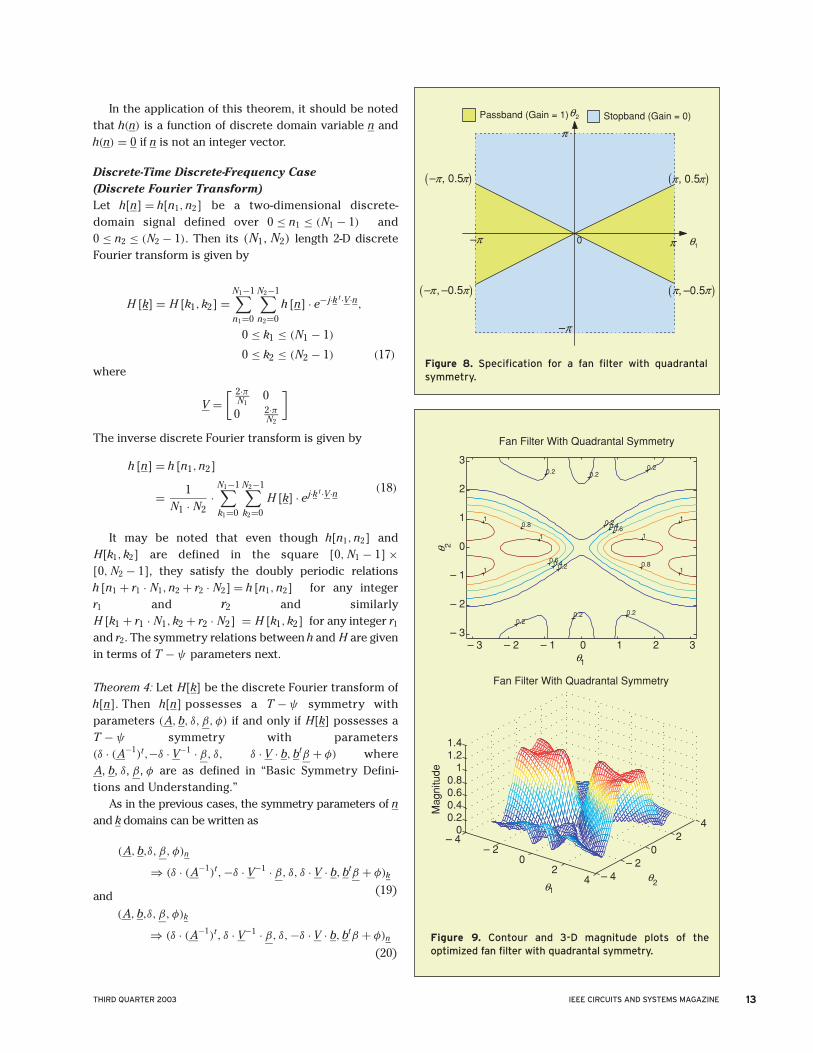
Figure 8. Specification for a fan filter with quadrantalsymmetry.

– 3 – 2 – 1 0 1 2 3– 3

– 2

– 1

0

1

2

30.2

0.2

0.2

0.2

0.2

0.2

0.2

0.20.4

0.4

0.6

0.60.8

0.8

1

1

1

1

1 1

1

2Fan Filter With Quadrantal Symmetry

θ

θ

– 4– 2

02

4 – 4– 2

02

40

0.20.40.60.8

11.21.4

2

Fan Filter With Quadrantal Symmetry

1

Mag

nitu

de

θθ

Figure 9. Contour and 3-D magnitude plots of the optimized fan filter with quadrantal symmetry.


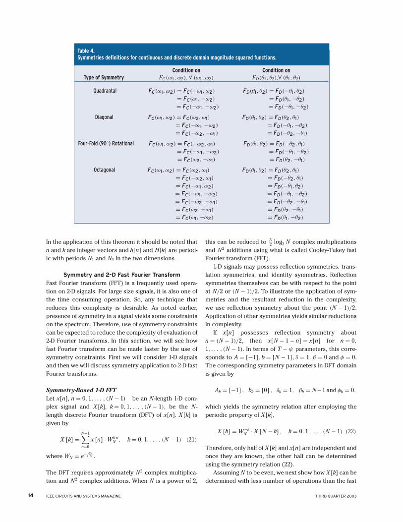
Condition on Condition on Type of Symmetry FC (ω1, ω2),∀ (ω1, ω2) FD(θ1, θ2),∀ (θ1, θ2)

Quadrantal FC(ω1, ω2) = FC(−ω1, ω2)

= FC(ω1,−ω2)

= FC(−ω1,−ω2)

FD(θ1, θ2) = FD(−θ1, θ2)

= FD(θ1,−θ2)

= FD(−θ1,−θ2)

Diagonal FC(ω1, ω2) = FC(ω2, ω1)

= FC(−ω1,−ω2)

= FC(−ω2,−ω1)

FD(θ1, θ2) = FD(θ2, θ1)

= FD(−θ1,−θ2)

= FD(−θ2,−θ1)

Four-Fold (90◦) Rotational FC(ω1, ω2) = FC(−ω2, ω1)

= FC(−ω1,−ω2)

= FC(ω2,−ω1)

FD(θ1, θ2) = FD(−θ2, θ1)

= FD(−θ1,−θ2)

= FD(θ2,−θ1)

FC(ω1, ω2) = FC(ω2, ω1)

= FC(−ω2, ω1)

= FC(−ω1, ω2)

= FC(−ω1,−ω2)

= FC(−ω2,−ω1)

= FC(ω2,−ω1)

= FC(ω1,−ω2)

FD(θ1, θ2) = FD(θ2, θ1)

= FD(−θ2, θ1)

= FD(−θ1, θ2)

= FD(−θ1,−θ2)

= FD(−θ2,−θ1)

= FD(θ2,−θ1)

= FD(θ1,−θ2)

Table 4. Symmetries definitions for continuous and discrete domain magnitude squared functions.

In the application of this theorem it should be noted thatn and k are integer vectors and h[n] and H[k] are period-ic with periods N1 and N2 in the two dimensions.

Symmetry and 2-D Fast Fourier Transform

Fast Fourier transform (FFT) is a frequently used opera-tion on 2-D signals. For large size signals, it is also one ofthe time consuming operation. So, any technique thatreduces this complexity is desirable. As noted earlier,presence of symmetry in a signal yields some constraintson the spectrum. Therefore, use of symmetry constraintscan be expected to reduce the complexity of evaluation of2-D Fourier transforms. In this section, we will see howfast Fourier transform can be made faster by the use ofsymmetry constraints. First we will consider 1-D signalsand then we will discuss symmetry application to 2-D fastFourier transforms.

Symmetry-Based 1-D FFTLet x[n], n = 0, 1, . . . , (N − 1) be an N -length 1-D com-plex signal and X [k], k = 0, 1, . . . , (N − 1), be the N -length discrete Fourier transform (DFT) of x[n]. X [k] isgiven by

X [k] =N−1∑

n=0

x [n] · Wk·nN , k = 0, 1, . . . , (N − 1) (21)

where WN = e− j 2πN .

The DFT requires approximately N2 complex multiplica-tion and N2 complex additions. When N is a power of 2,

this can be reduced to N2 log2 N complex multiplications

and N2 additions using what is called Cooley-Tukey fastFourier transform (FFT).

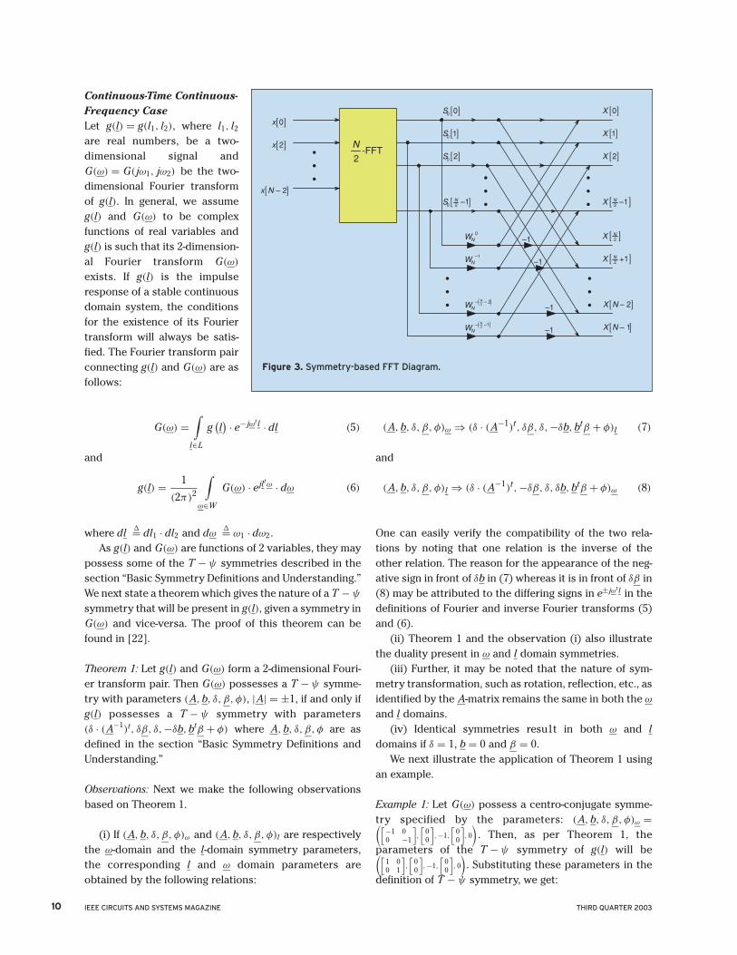
1-D signals may possess reflection symmetries, trans-lation symmetries, and identity symmetries. Reflectionsymmetries themselves can be with respect to the pointat N/2 or (N − 1)/2. To illustrate the application of sym-metries and the resultant reduction in the complexity, we use reflection symmetry about the point (N − 1)/2.Application of other symmetries yields similar reductionsin complexity.

If x[n] possesses reflection symmetry aboutn = (N − 1)/2, then x[N − 1 − n] = x[n] for n = 0,

1, . . . , (N − 1). In terms of T − ψ parameters, this corre-sponds to A = [−1], b = [N − 1], δ = 1, β = 0 and φ = 0.The corresponding symmetry parameters in DFT domainis given by

Ak = [−1] , bk = [0] , δk = 1, βk = N −1 and φk = 0,

which yields the symmetry relation after employing theperiodic property of X [k],

X [k] = W−kN · X [N − k] , k = 0, 1, . . . , (N − 1) (22)

Therefore, only half of X [k] and x[n] are independent andonce they are known, the other half can be determinedusing the symmetry relation (22).

Assuming N to be even, we next show how X [k] can bedetermined with less number of operations than the fast

Octagonal

Fourier transform. Using even and odd sample decompo-sition we can write X [k] as

X [k] =N−1∑

n = 0n even

x [n] · Wk·nN +

N−1∑n = 0n odd

x [n] · Wk·nN

=N2 −1∑r=0

x [2r] · Wk·2rN +

N2 −1∑r=0

x [2r + 1] · Wk·(2r+1)

N (23)

= S0 [k] + WkN · S1 [k]

where S0 and S1 are N/2 point DFTs. Now using the sym-metry properties x[N − 1 − n] = x[n], we can write S1 [k]in terms of S0[k] as

S1 [k] = W−2kN · S0

[ N2 − k

](24)

So for k = 0, 1, 2, . . . , N2 − 1,

X [k] = S0 [k] + WkN · W−2k

N · S0[ N

2 − k]

= S0 [k] + W−kN · S0

[ N2 − k

]

X[ N

2 + k] = S0 [k] − W−k

N · S0[ N

2 − k]

(25)

Thus X [k] for k = 0, 1, 2, . . . , (N − 1) can be determinedusing N/2 even indexed samples. This is illustrated in theflow diagram shown in Figure 3 on page 10.

It is noted that we need only one N2 -point FFT instead

of the normal two. As a result, the total number of com-plex multiplications needed is reduced to N

4 log2

( N2

) + N2

instead of N2 log2 N in the non-symmetrical case. Thus use

of symmetry results in approximately 50% reduction inthe computational complexity.

2-D SymmetriesAs in the 1-D case, symmetry can be utilized to reducethe computational complexity of 2-D discrete Fouriertransforms. In the following, we illustrate the symmetryapplication for centro symmetry and quadrantal symme-try cases.

As in the 1-D case, the reflection and rotation sym-metries can be defined with respect to

( N2 , N

2

)point or( N−1

2 , N−12

)point. Because of periodicity of h, the sym-

metries with respect to ( N

2 , N2

)will also correspond to

symmetries with respect to the origin (0, 0) for theperiodically extended signal. On the other hand, withthe choice of

( N−12 , N−1

2

)point for reflection or rotation,

the various symmetries will occur for h[n] with respectto the center of the given data. In the following,( N−1

2 , N−12

)is chosen in the definition of various sym-

metries for h[n].

Centro symmetry about (N−1

2 , N−12

)

An N × N array 2-D signal x[m,n] is said to possess cen-

tro symmetry about ( N−1

2 , N−12

)if

x[N −1−m, N −1−n] = x[m,n] for 0 ≤ m,n ≤ N −1

The corresponding symmetry relation for its 2-D discreteFourier transform X [k, l] is given by

X [N − k, N − l] = Wk+lN · X [k, l] (26)

Now employing the even-indexed and odd-indexed sam-ples decomposition, X [k, l] can be written as

X [k, l] = S00 [k, l] + WkN · S10 [k, l]

+ WlN · S01 [k, l] + Wk+l

N · S11 [k, l](27)

where

S00 [k, l] =N2 −1∑p =0

p even

N2 −1∑q = 0q even

x [2p, 2q] · Wk·p+l·qN2

S10 [k, l] =N2 −1∑

p=0

N2 −1∑

q=0

x [2p + 1, 2q] · Wk·p+l·qN2

S01 [k, l] =N2 −1∑

p=0

N2 −1∑

q=0

x [2p, 2q + 1] · Wk·p+l·qN2

S11 [k, l] =N2 −1∑

p=0

N2 −1∑

q=0

x [2p + 1, 2q + 1] · Wk·p+l·qN2

Now applying the symmetry relation we can write

S01 [k, l] = W−2(k+l)N · S10

[ N2 − k, N

2 − l]

and

S11 [k, l] = W−2(k+l)N · S00

[ N2 − k, N

2 − l]

Then,X [k, l] = S00 [k, l] + Wk

N · S10 [k, l]+ W−2k−l

N · S10[ N

2 − k, N2 − l

]

+ W−(k+l)N · S00

[ N2 − k, N

2 − l] (28)

From the above expression it is seen that when the cen-tro symmetry relation is employed, we need to computeonly two

(N2 × N

2

)size 2-D FFTs instead of four

(N2 × N

2

)

size 2-D FFTs. Thus there is a 50% reduction in the com-putational complexity.

Quadrantal symmetryA 2-D array x[m,n] is said to possess quadrantal symme-try if the following condition is satisfied:

x [m,n] = x [N − 1 − m,n] = x [m, N − 1 − n]

= x [N − 1 − m, N − 1 − n] (29)



Discrete domain(Note that xi = zi + z−1

i and yi = zi − z−1i ,

Continuous domain i = 1, 2)

Centro Symmetry Centro SymmetryP (s1, s2) · P (−s1,−s2)

=m1∑

i=0

n1∑

j=0

aijs2i1 s2j

2 + s1s2

m2∑

i=0

n2∑

j=0

bijs2i1 s2j

2

Q (z1, z2) · Q(z−1

1 , z−12

)

=m1∑

i=0

n1∑

j=0

cijxi1x

j2 + y1y2

m2∑

i=0

n2∑

j=0

dijxi1x

j2

Quadrantal Symmetry Quadrantal Symmetry

P (s1, s2) · P (−s1,−s2) =m1∑

i=0

n1∑

j=0

aijs2i1 s2j

2 Q (z1, z2) · Q(z−1

1 , z−12

) =m1∑

i=0

n1∑

j=0

cijxi1x

j2

Diagonal Symmetry Diagonal SymmetryP (s1, s2) · P (−s1,−s2)

=m1∑

i=0

n1∑

j=0

aijs2i1 s2j

2 + s1s2

m2∑

i=0

n2∑

j=0

bijs2i1 s2j

2

Q (z1, z2) · Q(z−1

1 , z−12

)

=m1∑

i=0

n1∑

j=0

cijxi1x

j2 + y1y2

m2∑

i=0

n2∑

j=0

dijxi1x

j2

where aij = aji and bij = bji. where cij = cji and dij = dji.

Four-Fold (90◦) Rotational Symmetry Four-Fold (90◦) Rotational SymmetryP (s1, s2) · P (−s1,−s2)

=m1∑

i=0

n1∑

j=0

aijs2i1 s2j

2 + s1s2

m2∑

i=0

n2∑

j=0

bijs2i1 s2j

2

Q (z1, z2) · Q(z−1

1 , z−12

)

=m1∑

i=0

n1∑

j=0

cijxi1x

j2 + y1y2

m2∑

i=0

n2∑

j=0

dijxi1x

j2

where aij = aji and bij = −bji. where cij = cji and dij = −dji.

Octagonal Symmetry Octagonal SymmetryP (s1, s2) · P (−s1,−s2) =

m1∑

i=0

n1∑

j=0

aijs2i1 s2j

2 Q(z1, z2) · Q(z−1

1 , z−12

) =m1∑

i=0

n1∑

j=0

cijxi1x

j2

where aij = aji. where cij = cji.

Table 5. Spectral forms of magnitude squared function for various symmetries.

It may be noted that quadrantal symmetry is defined herewith respect to the center of the array,

( N−12 , N−1

2

). In the

expression (29) for X [k, l], S10[k, l], S01[k, l] and S11[k, l]can be expressed in terms of S00[k, l] as shown next.

S10 [k, l] =N2 −1∑

p=0

N2 −1∑

q=0

x [2p + 1, 2q] · Wp·k+q·lN2

= W−2kN · S00

[ N2 − k, l

]

S01 [k, l] = W−2lN · S00

[k, N

2 − l]

and

S11 [k, l] = W−2(k+l)N · S00

[ N2 − k, N

2 − l]

Then X [k, l] can be written in terms of S00 solely as

X [k, l] = S00 [k, l] + W−kN · S00

[ N2 − k, l

]

+ W−lN · S00

[k, N

2 − l]

+ W−(k+l)N · S00

[ N2 − k, N

2 − l] (30)

It is then noted that evaluation of X [k, l] require the eval-uation of four N

2 × N2 size 2-D FFT’s when x[m,n] does not

possess any symmetry whereas only one N2 × N

2 size 2-DFFT is required when the quadrantal symmetry is presentin x[m,n]. In other words, utilization of the quadrantalsymmetry in x[m,n] reduces the computational com-plexity by approximately 75%. It may also be noted that

quadrantal symmetry in x[m,n] as defined in (29) resultsin a form of quadrantal symmetry in X [k, l] as

X [k, l] = W−kN · X [N − k, l] = W−l

N · X [k, N − l]= W−(k+l)

N · X [N − k, N − l](31)

Symmetrical Decomposition ForData Without SymmetryIn many situations, signals do not possess any symme-tries. In those cases, symmetry results cannot be appliedif we process the signals as they are. One way of dealingwith this situation is to decompose the signal into signalspossessing symmetries and anti-symmetries. For exam-ple, x[m,n] can be decomposed as

x [m,n] = x00 [m,n] + x10 [m,n]+ x01 [m,n] + x11 [m,n]

(32)

where x00 possesses quadrantal symmetry, x10 possessesquadrantal anti-symmetry of type 1 (anti-symmetry w.r.t.m and symmetry w.r.t. n), x01 possesses quadrantal anti-symmetry of type 2 (symmetry w.r.t. m and anti-symme-try w.r.t. n), and x11 possesses quadrantal anti-symmetryof type 3 (anti-symmetry w.r.t. both m and n).

Then each component can be processed using appro-priate symmetry properties. While this method may not

reduce the overall complexity, it will facilitate parallelprocessing of major computations.

Symmetry in 2-D Magnitude Response

In the design of two-dimensional filters, the design speci-fications are usually given in terms of the magnitude spec-trum which possesses certain symmetries, while thephase characteristic is either not known or is not impor-tant. In such cases, it is desirable to know the types oftransfer functions that can support the specified symme-try in the magnitude response. In this section, we willpresent the constraints on the numerator and denomina-tor polynomials of the transfer function, in order for themto possess the required symmetry and stability.

2-D Magnitude Response—Continuous and DiscreteRecall that the ψ operation only affects the phase of thefrequency response and not the magnitude. Hence, whendealing with magnitude symmetry, we assume ψ = ψ I

and call our T − ψ symmetry as simply T -symmetry.Now, in order for the magnitude response of a transferfunction to possess a particularly symmetry, both thenumerator and denominator polynomials have to pos-sess the symmetry individually. In other words, whenstudying the symmetry constraints on the transfer func-tion, one need only focus on the polynomial symmetryconstraints on the numerator and denominator. Thisobservation is a consequence of the following theorem.

Theorem 5: Let FC (ω) = P(ω)/D(ω) be a magnitudesquared function where P(ω) and D(ω) are relativelyprime polynomials. If FC (ω) possesses a T−symmetry,then P(ω) and D(ω) should possess the same T -symme-try individually.

It is to be noted that Theorem 5 also holds for discrete-domain cases, with appropriate change of variables.

Continuous-domain magnitude responseLet P(s1, s2) be a continuous domain polynomial. Then itsfrequency response P( jω1, jω2) is obtained by evaluatingthe polynomial on the imaginary axes of the (s1, s2)

biplane as shown in Figure 4 on page 11. Here, ω1 and ω2

denote the real frequency variables in the two-dimen-sional frequency plane: W 2 = W1 × W2.

If P(s1, s2) only has real coefficients, then the magni-tude-squared function FC (ω1, ω2), defined over the entireW 2 plane, is given by:

FC (ω1, ω2) = |P( jω1, jω2)|2= P( jω1, jω2) · P(− jω1,− jω2) (33)

From (33), it is easy to see that the magnitude squaredfunction is an even function in both ω1 and ω2, i.e.FC (ω1, ω2) = FC (−ω1,−ω2). So it should always be

expressible as the following general form:

FC (ω1, ω2) = FC 1(ω2

1, ω22

) + ω1ω2FC 2(ω2

1, ω22

)(34)

Applying analytic continuation to (33) and (34), we canwrite:

P(s1, s2) · P(−s1,−s2) = FC 1(s2

1, s22

) + s1s2FC 2(s2

1, s22

)(35)

One can observe that the magnitude squared function isa rational function in s1 and s2. This is the reason why wechoose to work with the magnitude squared functionrather than the magnitude function which is not rational.

Discrete-domain magnitude responseFor the discrete domain case, assuming that the polyno-mial is Q(z1, z2), its frequency response Q(e− jθ1, e− jθ2) isobtained by evaluating the polynomial on the boundaryof the unit circles in the (z1, z2) biplane as shown in Figure 5 on page 11. The discrete-domain frequency vari-ables θ1 and θ2 are related to the continuous-domain onesthrough θ1 = ω1 · T and θ2 = ω2 · T , where T is the sam-pling period in both directions.

If Q(z1, z2) possesses only real coefficients, then themagnitude-squared function FD(θ1, θ2) is obtained by:

FD(θ1, θ2) = |Q(e− jθ1, e− jθ2)|2= Q(e− jθ1, e− jθ2) · Q(ejθ1, ejθ2) (36)

Once again, it is easy to see that the magnitude squaredfunction is an even function, i.e. FD(θ1, θ2) =FD(−θ1,−θ2). As such, it should be expressible as:

FD(θ1, θ2) =FD1(cos θ1, cos θ2)

+ sin θ1 · sin θ2 · FD2(cos θ1, cos θ2) (37)

It should be obvious that, in the above, cos(θi) is even andsin (θi) is odd.

Using analytic continuation, we have:

Q(z1, z2) · Q(z−1

1 , z−12

)

= FD1(z1 + z−1

1 , z2 + z−12

) + (z1 − z−1

1

) · (z2 − z−12

)

· FD2(z1 + z−1

1 , z2 + z−12

)(38)

Equations (35) and (38) give the spectral forms of themagnitude squared functions for the continuous domainand discrete domain cases respectively.

Bilinear transformation between 2-D continuous anddiscrete variablesThe double bilinear transformation si = (1 − zi)/(1 + zi),i = 1, 2 is often used to generate a 2-D discrete domainfunction from a 2-D continuous domain function. Theadvantage of this method is that the symmetry present in


the continuous domain magnitude response is carriedover to the discrete domain magnitude response. The fol-lowing is a simple proof. Assume,

FD(z1, z2) = FC (s1, s2)|si=(1−zi)/(1+zi), i = 1, 2

In terms of the frequency variables, this can be expressedas:

FD(θ1, θ2) = F (ω1, ω2)|ωi=tan(θi/2), i = 1, 2

Now if FC (s1, s2) possesses, say, 4-fold rational symmetry,then

FC (ω1, ω2) ≡ FC (−ω2, ω1)

So,

FD(θ1, θ2) ≡ FC (− tan(θ2/2), tan(θ1/2))

≡ FD(−θ2, θ1)

Therefore, the discrete domain magnitude squared func-tion obtained through bilinear transformation possessesthe same 4-fold rational symmetry present in the originalcontinuous domain function. It can be shown that thisresult holds for the other symmetries as well. We sum-marize in Table 4 on page 14 the symmetry conditions forour magnitude squared functions in both continuous anddiscrete domains.

Spectral FormsIn this section, we present the constraints on the magni-tude squared function in order for it to possess the vari-ous symmetries. Recall that for a continuous or discretedomain transfer function with real coefficients, its magni-tude squared function is always an even function. Focus-ing on the continuous domain case, this meansFC (ω1, ω2) = FC (−ω1,−ω2). As such, the magnitudesquared function always possesses centro symmetry, andis expressible as (34). Now, if FC (ω1, ω2) also possessesquadrantal symmetry, then FC (ω1, ω2) = FC (ω1,−ω2).Using (34), this can be written as:

FC 1(ω2

1, ω22

)+ω1ω2FC 2(ω2

1, ω22

)

=FC 1(ω2

1, ω22

) − ω1ω2FC 2(ω2

1, ω22

)(39)

The above is only possible if FC 2(ω21, ω

22) = 0. Thus,

FC (ω1, ω2) = FC 1(ω21, ω

22). So the spectral form for the

magnitude squared function that possesses quadrantalsymmetry is:

P(s1, s2) · P(−s1,−s2) = FC 1(s2

1, s22

)

=m1∑

i=0

n1∑

j=0

aijs2i1 s2 j

2 (40)

We can use the same procedure to obtain the spectralforms for the other symmetries in continuous as well asdiscrete domains. These spectral forms are listed in Table 5 on page 16.

Polynomial SymmetryIn order for a transfer function to possess various magni-tude symmetries, the numerator and denominator poly-nomials have to possess the same symmetriesindividually. So, we now consider the symmetry con-straints on the polynomials. We first introduce the fol-lowing key theorem:

Theorem 6 (Unique factorization theorem for multivariablepolynomial) [23]: A multivariable polynomial can be fac-tored into a set of irreducible polynomials and the factorsare unique within a multiplicative constant. In otherwords, let P(ω) be factored in two ways as the left-, andright-hand sides of the following identity:

K1

I1∏

i=1

Pi(ω) ≡ K2

I2∏

i=1

Qi(ω)

where all Pi(ω)’s and Qi(ω)’s are irreducible polynomials.Then, it is required that I1 = I2 = I and for each Pi(ω),i = 1, 2, . . . , I, there exists a unique Qj(ω) (i may be equalto j) such that

Pi(ω) = kjQj(ω)

where kj’s are constants such that K2 = K1

I∏j=1

kj.

Using the unique factorization theorem, we can obtainthe polynomial factors that satisfy the various symme-tries. For example, for quadrantal symmetry, its magni-tude squared function has to satisfy FC (ω1, ω2) =FC (ω1,−ω2), i.e.

P( jω1, jω2) · P(− jω1,− jω2) = P( jω1,− jω2) · P(− jω1, jω2)

Using analytic continuation, this becomes:

P(s1, s2) · P(−s1,−s2) = P(s1,−s2) · P(−s1, s2) (41)

If we assume P(s1, s2) to be irreducible, the unique factor-ization theorem of multivariable polynomials states thatP(s1, s2) should satisfy one of the following two conditions:

(i)P(s1, s2)=k1 · P(s1,−s2)wherek1 is a real constant. (42)

(ii)P(s1, s2)=k2 ·P(−s1, s2)where k2 is a real constant. (43)

It is easy to see that for case (i), P needs to be even in s2,and for case (ii), P needs to be even in s1. Therefore, the


polynomial factors satisfying quadrantal symmetry are:P(s1, s2

2

)and P

(s2

1, s2). More factors can be derived if we

assume P to be reducible. These are P(s1, s2) · P(s1,−s2)

and P(s1, s2) · P(−s1, s2).In Table 6 above we state the continuous and discrete

domain polynomial factors that posses the various sym-metries. These factors are derived using the procedurejust discussed. It is to be noted that for the polynomial

factors listed under each symmetry, their products pos-sess the same symmetry as well. For example, P1

(s1, s2

2

)

and P2(s2

1, s2)

each possess quadrantal symmetry. So theirproduct P1

(s1, s2

2

) · P2(s2

1, s2)

possesses quadrantal sym-metry as well.

Symmetry and StabilityFor a transfer function to possess symmetry, the denom-


Discrete domain(Note that xi = zi + z−1

i and yi = zi − z−1i

Continuous domain for i = 1, 2)

Quadrantal Symmetry Quadrantal Symmetry

a) P(s1, s2

2

)a) Q (z1, x2)

b) P(s2

1 , s2)

b) Q (x1, z2)

c) P (s1, s2) · P (s1,−s2) c) Q (z1, z2) · Q(z1, z−1

2

)

d) P (s1, s2) · P (−s1, s2) d) Q (z1, z2) · Q(z−1

1 , z2)

Diagonal Symmetry Diagonal Symmetry

a) P1 (s1, s2) a) Q1 (z1, z2)

b) P2(s2

1 , s22

) + s1s2P3(s2

1 , s22

)b) Q2 (x1, x2) + y1y2Q3 (x1, x2) + y1Q4 (x1, x2)

+ s1P4(s2

1 , s22

) − s2P4(s2

2, s21

) − y2Q4 (x2, x1)

c) P (s1, s2) · P (s2, s1) c) Q (z1, z2) · Q (z2, z1)

d) P (s1, s2) · P (−s2,−s1) d) Q (z1, z2) · Q(z−1

2 , z−11

)

where where

P1 (s1, s2) = P1 (s2, s1) and Q1 (z1, z2) = Q1 (z2, z1) and

Pk(s2

1 , s22

) = Pk(s2

2, s21

)for k = 2, 3. Qk (x1, x2) = Qk (x2, x1) for k = 2, 3.

Four-Fold (90◦) Rotational Symmetry Four-Fold (90◦) Rotational Symmetry

a) P1(s2

1 , s22

) + s1s2 · (s21 − s2

2

) · P2(s2

1 , s22

)a) Q1 (x1, x2) + y1y2 · (x1 − x2) · Q2 (x1, x2)

b) (s2

1 − s22

)P1

(s2

1 , s22

) + s1s2P2(s2

1 , s22

)b) (x1 − x2) Q1 (x1, x2) + y1y2Q2 (x1, x2)

c) P (s1, s2) · P (−s2, s1) c) Q (z1, z2) · Q(z−1

2 , z1)

d) P (s1, s2) · P (s2,−s1) d) Q (z1, z2) · Q(z2, z−1

1

)

e) P (s1, s2) · P (−s2, s1) e) Q (z1, z2) · Q(z−1

2 , z1)

× P (−s1,−s2) · P (s2,−s1) ×Q(z−1

1 , z−12

) · Q(z2, z−1

1

)

where where

Pk(s2

1 , s22

) = Pk(s2

2, s21

)for k = 1, 2. Qk (x1, x2) = Qk (x2, x1) for k = 1, 2.

Octagonal Symmetry Octagonal Symmetry

a) (s2

1 − s22

)α · P1(s2

1 , s22

), where α = 0 or 1. a) (x1 − x2)α · Q1 (x1, x2), where α = 0 or 1.

b) P(s2

1 , s2) · P

(s2

2, s1)

b) Q (x1, z2) · Q (x2, z1)

c) P(s2

1 , s2) · P

(s2

2,−s1)

c) Q (x1, z2) · Q(x2, z−1

1

)

d) P(s1, s2

2

) · P(−s2, s2

1

)d) Q (z1, x2) · Q

(z−1

2 , x1)

e) P2 (s1, s2) · P2 (−s1, s2) e) Q2 (z1, z2) · Q2(z−1

1 , z2)

f) P2 (s1, s2) · P2 (s1,−s2) f) Q2 (z1, z2) · Q2(z1, z−1

2

)

where where

P1(s2

1 , s22

) = P1(s2

2, s21

)and Q1 (x1, x2) = Q1 (x2, x1) and

P2 (s1, s2) = P2 (s2, s1). Q2 (z1, z2) = Q2 (z2, z1) .

Table 6. Continuous and discrete domain polynomial factors possessing symmetry.

inator polynomial D(s1, s2) has to satisfy the conditionsfor the symmetry as well as stability. So there is an addi-tional stability constraint on the denominator polynomialcompared to the numerator polynomial. It has beenshown in [17, 24–26] that the sufficient condition for 2-Dcontinuous domain filters to be stable is that their trans-fer functions do not have any poles in the region of the(s1, s2) biplane defined by Re(s1) ≥ 0 and Re(s2) ≥ 0,including infinite distant points. Similarly, a sufficient con-dition for the stability of 2-D discrete domain filters is thattheir transfer functions do not have any poles in theregion of the (z1, z2) biplane defined by |z1| ≤ 1 and|z2| ≤ 1. Continuous domain and discrete domain stabili-ty results are related by the double bilinear transforma-tion, si = (1 − zi)/(1 + zi), i = 1, 2. Applying thesestability conditions on the polynomial factors that pos-sess the various magnitude symmetries, the conditionson the denominator polynomials of 2-D filters areobtained. These are listed in Table 7 on page 25. The inter-ested reader may refer to [20] for the details and theproof.

IIR Filter DesignThe design of filters involves the determination of the fil-ter coefficients such that the resulting magnituderesponse approximates the ideal specifications to a cer-tain tolerance. Design of 2-D digital filters is more compli-cated than 1-D digital filters because the increase indimension brings about an exponential increase in thenumber of coefficients. Fortunately, 2-D frequencyresponses possess many types of symmetries and thepresence of these symmetries can be used to reduce thecomplexity of the design. Symmetry present in the fre-


– 3 – 2 – 1 0 1 2 3– 3

– 2

– 1

0

1

2

3

0.2

0.2

0.2

0.2

0.2

0.2

0.2

0.2

0.4

0.4

0.4

0.4

0.4

0.4

0.6

0.6

0.6

0.6

0.6

0.6

0.6

0.6

0.6

0.6

0.6

0.6

0.6

0.8

0.8

0.8

0.8

1

1

1

1

1

1

1

1

1

θ

2θ

– 4– 2

02

4 – 4– 2

02

40

0.20.40.60.8

11.21.4

2

Fan Filter With 4-Fold Rotational Symmetry

1

Mag

nitu

de

θθ

Fan Filter With 4-Fold Rotational Symmetry

Figure 11. Contour and 3-D magnitude plots of the opti-mized fan filter with 4-fold rotational symmetry.

Stopband (Gain = 0) Passband (Gain = 1)

1θ

2θ

π

π– π

π–

0

( ), 0.5–π π

( )π π

( )0.5 ππ,

( )ππ –,

0.5–,

0.5–

Figure 10. Specification for a fan filter with 4-fold (90◦)rotational symmetry.

Stopband (Gain = 0)

Passband (Gain = 1)

1θ

π

π

π– π

1

1–1–22

2

0

–1

–2

θ2

Figure 12. Specification for a bandpass filter with octago-nal symmetry.

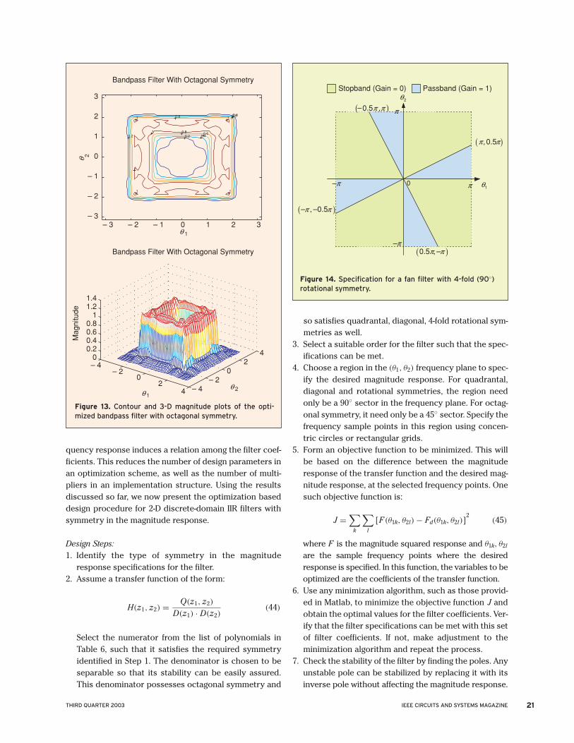
quency response induces a relation among the filter coef-ficients. This reduces the number of design parameters inan optimization scheme, as well as the number of multi-pliers in an implementation structure. Using the resultsdiscussed so far, we now present the optimization baseddesign procedure for 2-D discrete-domain IIR filters withsymmetry in the magnitude response.

Design Steps:1. Identify the type of symmetry in the magnitude

response specifications for the filter.2. Assume a transfer function of the form:

H(z1, z2) = Q(z1, z2)

D(z1) · D(z2)(44)

Select the numerator from the list of polynomials inTable 6, such that it satisfies the required symmetryidentified in Step 1. The denominator is chosen to beseparable so that its stability can be easily assured.This denominator possesses octagonal symmetry and

so satisfies quadrantal, diagonal, 4-fold rotational sym-metries as well.

3. Select a suitable order for the filter such that the spec-ifications can be met.

4. Choose a region in the (θ1, θ2) frequency plane to spec-ify the desired magnitude response. For quadrantal,diagonal and rotational symmetries, the region needonly be a 90◦ sector in the frequency plane. For octag-onal symmetry, it need only be a 45◦ sector. Specify thefrequency sample points in this region using concen-tric circles or rectangular grids.

5. Form an objective function to be minimized. This willbe based on the difference between the magnituderesponse of the transfer function and the desired mag-nitude response, at the selected frequency points. Onesuch objective function is:

J =∑

k

∑

l

[F (θ1k, θ2l) − Fd(θ1k, θ2l)]2

(45)

where F is the magnitude squared response and θ1k, θ2l

are the sample frequency points where the desiredresponse is specified. In this function, the variables to beoptimized are the coefficients of the transfer function.

6. Use any minimization algorithm, such as those provid-ed in Matlab, to minimize the objective function J andobtain the optimal values for the filter coefficients. Ver-ify that the filter specifications can be met with this setof filter coefficients. If not, make adjustment to theminimization algorithm and repeat the process.

7. Check the stability of the filter by finding the poles. Anyunstable pole can be stabilized by replacing it with itsinverse pole without affecting the magnitude response.


– 3 – 2 – 1 0 1 2 3– 3

– 2

– 1

0

1

2

3

0.2 0.2

0.4

0.4

0.6

0.6

0.8

0.8

1

1

1

1

1

1

1

2Bandpass Filter With Octagonal Symmetry

θ

θ

– 4– 2

02

4 – 4– 2

02

40

0.20.40.60.8

11.21.4

Bandpass Filter With Octagonal Symmetry

Mag

nitu

de

21θ

θ

Figure 13. Contour and 3-D magnitude plots of the opti-mized bandpass filter with octagonal symmetry.

Stopband (Gain = 0) Passband (Gain = 1)

1θ

2θ( )

π

π–

( )

( )

π

π–

( )

0

0.5–π π–

0.5 ππ –,

0.5ππ,

0.5 ππ ,–

,

Figure 14. Specification for a fan filter with 4-fold (90◦)rotational symmetry.

Example 4: Using the procedure just discussed, we nowdesign a bandpass filter with the filter specificationshown in Figure 6.

It can be seen that the filter possesses diagonal sym-metry. So we select the numerator to be Q(z1, z2) =Q(z2, z1), which is Case (a) in the list of polynomialswith diagonal symmetry in Table 6. We pick the order of

the filter to be 4×4. The following are the forms for thenumerator and denominator. It can be seen that thenumerator coefficient matrix has diagonal symmetry. Asa result, the number of variables to optimize is reducedfrom 50 (25 for the numerator and 25 for the denomina-tor) to 19 (15 for the numerator and 4 for the denomina-tor), a 62% reduction.

z02 z1

2 z22 z3

2 z42

Q(z1, z2) =

z01

z11

z21

z31

z41

a00 a01 a02 a03 a04

a01 a11 a12 a13 a14

a02 a12 a22 a23 a24

a03 a13 a23 a33 a34

a04 a14 a24 a34 a44

(46)

and

D(zi) = b0 + b1zi + b2z2i + b3z3

i + z4i , i = 1, 2

We use the “lsqnonlin” routine in Matlab 5.3’s Optimiza-tion Toolbox to minimize the objective function. Becauseof symmetry, we need only specify the desired responsein a reduced region (90◦ sector) in the frequency plane.The transfer function coefficients of the optimized filterare listed on page 23, with the contour and 3-D magnitudeplots given in Figure 7 on page 12. We verified that the fil-ter is stable and meets the specification.


– 3 – 2 – 1 0 1 2 3– 3

– 2

– 1

0

1

2

3

0.2

0.2

0.2

0.2

0.2

0.2

0.2

0.2

0.4

0.4

0.40.4

0.6

0.6

0.6

0.6

0.8

0.8

0.8

0.8

1

1

1

1

1

2

FIR Fan Filter With 4-Fold Rotational Symmetry

θ

θ

– 4– 2

02

4 – 4

– 2

0

2

40

0.2

0.4

0.6

0.8

1

1.2

1.4

FIR Fan Filter With 4-Fold Rotational Symmetry

Mag

nitu

de2

1θθ

Figure 15. Contour and 3-D magnitude plots of the optimized FIR filter with 4-fold rotational symmetry.

Stopband (Gain = 0)Passband (Gain = 1)

1θ

2θ

π

( )

π–

( )( ),

( )

ππ– 0

π–π– / 3

,ππ– / 3

, π–π / 3

,ππ / 3

Figure 16. Fan filter specification.


a00 = 0.05691572886174

a01 = −0.02461862190217

a02 = 0.00986568924226

a03 = −0.01034804473379

a04 = 0.05820287661798

a11 = −0.02118017629239

a12 = −0.00404160157329

a13 = 0.03303916563349

a14 = −0.01033357674522

a22 = 0.00255022502754

a23 = −0.00398097317269

a24 = 0.00985123577827

a33 = −0.02118784417373

a34 = −0.02462035270181

a44 = 0.05691802180139

b0 = 0.45583704915947

b1 = −0.09763672454601

b2 = 0.87533799314168

b3 = −0.03923759607499

Other types of filters can be designed using the sameprocedure. The following are some more examples.

Example 5: The filter specification in Figure 8 on page 13possesses quadrantal symmetry. So we select the transferfunction numerator to beQ1(z1, z2 + z−1

2 ) · Q2(z1 + z−11 , z2). This is the product of

Case (a) and (b) in the list of polynomials with quadrantal

symmetry in Table 6. The filter order is chosen to be 4 × 4.The transfer function can be expressed as:

The following are the optimized filter coefficients.Because of the quadrantal symmetry constraints, thenumber of independent variables to optimize is reducedfrom 50 to 16 (12 for the numerator and 4 for the denom-inator), a 68% reduction. The resulting contour and 3-Dplots are shown in Figure 9 on page 13.

a00 = −0.36223343641959

a10 = 0.73781886914067

a20 = −0.35115585228984

a01 = 0.18001689678736

a11 = −0.23263738256684

a21 = 0.18813447360982

b00 = 0.49109027165487

b01 = 0.31981445338169

b02 = 0.49120885907429

b10 = −0.11409694648059

b11 = −0.38504269416613

b12 = −0.11398910827760

d0 = −0.02550110734351

d1 = −0.01599046367101

d2 = 0.37661874629072

d3 = −1.06746935205100

Example 6: It can be observed that the filter specificationin Figure 10 on page 20 possesses 4-fold (90◦) rotationalsymmetry. So, we select the transfer function numeratorto be Q(z1, z2) · Q(z2, z−1

1 ), which is Case (d) for polyno-mials with 4-fold rotational symmetry in Table 6. The fil-ter order is chosen to be 5×5 and the transfer functioncan be written as:

H(z)

=Q1

(z1, z2 + z−1

2

)· Q2

(z1 + z−1

1 , z2

)D(z1) · D(z2)

=

(2∑

m=0

1∑n=0

amn · zm1 ·

(z2 + z−1

2

)n)

·(

1∑m=0

2∑n=0

bmn ·(z1 + z−1

1

)m · zn2

)(

z41 +

3∑i=0

dizi1

)·(

z42 +

3∑i=0

dizi2

)

= 0

= 0.5

1θ

2θ

( )

( )( )

( )

( )( )

( )( )

π

ππ–

π–

0

,π– π/ 3

,ππ / 3

, π–π / 3

,π π–/ 3,π– π–/ 3

, π–π– / 3

,ππ– / 3

,π π/ 3

Figure 17. Octagonally symmetrical component ofresponse.

H(z) = Q(z1, z2) · Q(z2, z−1

1 )

D(z1) · D(z2)

=

(4∑

m=0

1∑n=0

amn zm1 zn

2

)·(

4∑m=0

1∑n=0

amn zm2 z−n

1

)(

z51 +

4∑i=0

d i zi1

)·(

z52 +

4∑i=0

d i zi2

)

The following are the optimized filter coefficients. Here, thenumber of independent variables to optimize is reducedfrom 72 to 15 (10 for the numerator and 5 for the denomi-nator), a 79% reduction. The resulting contour and 3-D per-spective plots are shown in Figure 11 on page 20.

a00 = 0.20294324476412

a01 = −0.48163632801449

a10 = 0.36932528231741

a11 = 0.18286723039587

a20 = −0.60107454130023

a21 = 0.57969763481886

a30 = −0.08314333950507

a31 = −0.32680233587436

a40 = 0.12928331110133

a41 = −0.02087010625653

d0 = 0.03480848557051

d1 = −0.34376565481538

d2 = 0.76070962863907

d3 = −0.08613899671423

d4 = −1.31455055755094

Example 7: In this example, we are required to design afilter to meet the specifications given in Figure 12 onpage 20.

It can be seen that the response possesses octagonalsymmetry. So using Table 6 and assuming the filter orderto be 6 × 6, we can write the transfer function as:

The transfer function numerator chosen is Case (b) in thelist of polynomials with octagonal symmetry.

Here, the advantage of employing the symmetry con-straints is that the number of independent coefficients tooptimize is reduced from 98 to 16 (10 for the numeratorand 6 for the denominator), an 84% reduction. Also,because of octagonal symmetry, the optimization needonly be done in a reduced 45◦ degree sector in the fre-quency plane, which gives further reduction in computa-tional time. The optimized filter coefficients are shownbelow. The contour and 3-D plots of the optimized filterare shown in Figure 13 on page 21.

a00 = −0.02676667082778

a01 = −0.30824801305310

a02 = −0.61338664353594

a03 = −0.54784348150223

a04 = −0.23052991083493

a10 = −0.08712047342727

a11 = 0.10230094916767

a12 = 0.44881705473037

a13 = 0.53311155984782

a14 = 0.28348672960777

d0 = 0.07858008457571

d1 = −0.10704620692704

d2 = 0.66811506285393

d3 = −0.19413076009780

d4 = 1.15029323700482

d5 = −0.09513351068716


= 0

= 0.5

1θ

2θ

( )

( )( )

( )

( )( )

( )( )

ππ–

π

π–

= – 0.5

0

,π– π/ 3 ,π π/ 3

,ππ / 3

, π–π / 3

,π π–/ 3,π– π–/ 3

, π–π– / 3

,ππ– / 3

Figure 18. Octagonally antisymmetrical component ofresponse.

H(z) =Q

(z1 + z−1

1 , z2

)· Q

(z2 + z−1

2 , z1

)D(z1) · D(z2)

=

(1∑

m=0

4∑n=0

amn ·(z1 + z−1

1

)m · zn2

)·(

1∑m=0

4∑n=0

amn ·(z2 + z−1

2

)m · zn1

)(

z61 +

5∑i=0

dizi1

)·(

z62 +

5∑i=0

dizi2

)


Continuous domain Discrete domain

Quadrantal Symmetry Quadrantal SymmetryD (s1, s2) = D1 (s1) · D2 (s2) D (z1, z2) = D1 (z1) · D2 (z2)

where D1 and D2 are stable 1-D polynomials. where D1 and D2 are stable 1-D polynomials.

Diagonal Symmetry Diagonal SymmetryD(s1, s2) = D(s2, s1) where D is stable. D(z1, z2) = D(z2, z1) where D is stable.

Four-Fold (90◦) Rotational Symmetry Four-Fold (90◦) Rotational SymmetryD (s1, s2) = D1 (s1) · D1 (s2) D (z1, z2) = D1 (z1) · D1 (z2)

where D1 is a stable 1-D polynomial. where D1 is a stable 1-D polynomial.

Octagonal Symmetry Octagonal SymmetryD (s1, s2) = D1 (s1) · D1 (s2) D (z1, z2) = D1 (z1) · D1 (z2)

where D1 is a stable 1-D polynomial. where D1 is a stable 1-D polynomial.

Table 7. Polynomial factors possessing symmetry and stability.

– 3 – 2 – 1 0 1 2 3– 3

– 2

– 1

0

1

2

3

0

0

0

0

0.1

0.1

0.1

0.1

0.2

0.2

0.2

0.2

0.3

0.3

0.3

0.3

0.3

0.4

0.4

0.4

0.4

0.5

0.5

0.5

0.5

1

2

Octagonally Symmetric Component

θ

θ

– 4– 2

02

4 – 4– 2

02

4– 0.1

00.10.20.30.40.50.6

Octagonally Symmetric Component

21θ

θ

Figure 19. Contour and 3-D plots of the symmetric component.

FIR Filter DesignJust like for IIR filters, symmetry can also be used toreduce the complexity in the design of 2-D finite impulseresponse (FIR) filters. The transfer function of a 2-D FIRfilter has the form

∑

m

∑

nhmn · zm

1 · zn2 , where the coeffi-

cients hmn are the impulse response samples. An FIR filtercan be designed to possess linear phase which makes itattractive in certain applications. However, the disadvan-tage is that it often requires a much higher filter order tosatisfy the same specification compared to an IIR filter.

In the following, we present an FIR design example uti-lizing symmetry. We use basically the same design stepspresented previously for IIR filters, except that step 7 isnot needed here since an FIR filter is always stable.

Example 8: The filter specification shown in Figure 14 onpage 21 possesses 4-fold (90◦) rotational symmetry. So,using Table 6, we write the filter transfer function as:

H(z1, z2) ={Q1(x1, x2) + y1y2 · (x1 − x2) · Q2(x1, x2)} · zα

1 · zα2 (47)

where Qk(x1, x2) = Qk(x2, x1) for k = 1, 2.This is Case (a) in the polynomials with rotational

symmetry. (The zα1 and zα

2 factors are included to ensurethe polynomial nature of H(z1, z2)). The polynomial in(47) is the result of the symmetry conditionH(z1, z2) = H(z−1

2 , z1) · zN2 . Consequently, the coeffi-

cients have to satisfy the condition hmn = hn,N−m, which

means that the coefficient matrix has to possess 4-fold(90◦) rotational symmetry. The coefficient matrix isshown below for a filter of impulse response (coefficient)size of 7×7. It can be seen that only the boxed coefficientsare independent, and the other coefficients can beobtained by rotating the boxed coefficients in steps of 90◦

around the mid-point of the whole matrix.

Because of the symmetry constraint, the number of inde-pendent coefficients is 13, a 73% reduction from the original49. The optimized filter coefficients are shown below and theresulting filter response is shown in Figure 15 on page 22.

a00 = −6.2016 × 10−3

a01 = −52.534 × 10−3

a02 = 45.586 × 10−3

a03 = 7.3391 × 10−3

a10 = 23.106 × 10−3

a11 = −32.25 × 10−3

a12 = 66.891 × 10−3

a13 = 52.406 × 10−3

a20 = −13.519 × 10−3

a21 = −78.678 × 10−3

a22 = −68.031 × 10−3

a23 = 49.386 × 10−3

a33 = 0.23983

It is to be noted that the choice of transfer functionhere results in a filter with linear phase. This is becauseon substituting zi = e− jθi into the transfer function, we get

H(θ1, θ2) = {Q1(cos θ1, cos θ2) + sin θ1 · sin θ2

× (cos θ1 − cos θ2) · Q2(cos θ1, cos θ2)}× e− jα·θ1 · e− jα·θ2

The expression {Q1(cos θ1, cos θ2) + sin θ1 · sin θ2·(cos θ1 − cos θ2) · Q2(cos θ1, cos θ2)} is real. Thus,�H(θ1, θ2) = −α · (θ1 + θ2) + k · π , where k is an integer,and so the phase is linear.

Symmetrical Decomposition and Transformation

Among the methods used in the design of 2-D FIR filters,optimization, window techniques, and transformation arethe most popular. In this section, we first present tech-niques to improve the efficiency and versatility of thetransformation method by making use of the symmetryproperties of the transformation functions. After that, wedescribe a procedure to extend the application of sym-metry properties to the design of filters that do not pos-sess identifiable symmetry in their frequency responses.The approach that is followed is to decompose the givenspecification into a number of components each possess-ing some form of symmetry.

1-D to 2-D TransformationAmong the various methods available for the design of 2-D FIR filters, transformation method has been found tobe the simplest and most efficient one for many specifi-cations. Introduced by McClellan in 1973, this methodhas been studied extensively by a number of researchworkers in this field. Here, we present techniques toimprove the efficiency and versatility of this method bymaking use of the symmetry properties of transforma-tion functions.

Let G(u) represent the frequency response of a 1-D FIR filter. Then G(u) can be written as

G(u) = g(0) +N∑

n=1

2 · g(n) · cos(nu) (48)


Name of Symmetry Condition on Symmetry Condition on Antisymmetry

Quadrantal bmn = 0 akl = 0

Diagonal akl = alk akl = −alk

bmn = bnm bmn = −bnm

Four-Fold (90◦) rotational akl = alk akl = −alk

bmn = −bnm bmn = bnm

Octagonal akl = alk i) akl = 0, bmn = bnm

bmn = 0 ii) akl = −alk, bmn = 0iii) akl = 0, bmn = −bnm

Table 8. Coefficient conditions for various symmetries on polynomial P (θ)in (52).

z02 z1

2 z22 z3

2 z42 z5

2 z62

H(z1, z2) =

z01

z11

z21

z31

z41

z51

z61

a00 a01 a02 a03 a20 a10 a00

a10 a11 a12 a13 a21 a11 a01

a20 a21 a22 a23 a22 a12 a02

a03 a13 a23 a33 a23 a13 a03

a02 a12 a22 a23 a22 a21 a20

a01 a11 a21 a13 a12 a11 a10

a00 a10 a20 a03 a02 a01 a00

where g(n) is the impulse response sequence of the 1-DFIR filter. Expressing cos(nu) in terms of cos(u), we canrewrite (48) as

G(u) =N∑

n=0

bn · (cosu)n = G(cosu) (49)

The generalized McClellan transformation which con-verts the 1-D zero phase FIR filter into a 2-D zero phaseFIR filter is given by

cosu = P(θ) = P(cos θ1, cos θ2, sin θ1, sin θ2) (50)

where P(θ) can be considered as the frequency responsefunction of a 2-D zero phase FIR filter. Substitution of (50)in (49) gives a 2-D zero phase frequency response func-tion as

H(θ) = G(P(θ)) = H(cos θ1, cos θ2, sin θ1, sin θ2) (51)

It may be easily verified that the response of H(θ) at apoint θ i is given by G(cos−1[P(θ i)]), i.e., the response ofG(u) at u = cos−1[P(θ i)]. This means that all those pointsin the (θ1, θ2) plane where P(θ) = P(θ i), the response willhave a constant value and the line joining these pointswill constitute a constant value contour. In other words,the response of the 1-D function G(u) is carried over tothe 2-D plane by the transformation (50). The actualresponse values of these contours are determined byG(u). Very often, the specified 2-D response possessessome form of symmetry in addition to being real, and theutilization of this symmetry will reduce the complexity ofthe filter design.

Symmetry constraints on transformation functionsFrom the previous discussion on the generation of 2-Dfunctions using transformation functions, it should beapparent that the symmetry properties of the generated 2-D function will depend on the symmetry properties of the1-D base function G(u) and the 2-D transformation functionP(θ). We will now investigate the natures of G(u) and P(θ)

such that the generated function H(θ) possesses a desiredT -symmetry or T -antisymmetry. In this context, we state anumber of theorems that outline these properties.

Theorem 7: If P(θ) possesses a T -symmetry, thenH(θ) = G(P(θ)) possesses the same T -symmetry inde-pendent of the nature of G(u).

Theorem 8: If P(θ) possesses a T -antisymmetry andG(u) = G(π − u), i.e., G(u) possesses a reflection symme-try about u = π/2, then H(θ) = G(P(θ)) possesses the T -symmetry. It is to be noted that G(u) = G(π − u) if it can be expressed as G(u) = ∑N

n=0 cn(cosu)2n.

Theorem 9: If P(θ) possesses a T -antisymmetry andG(u) = −G(π − u), i.e., G(u) possesses a reflection anti-symmetry about u = π/2, then H(θ) = G(P(θ)) possessesthe T -antisymmetry. It is to be noted that G(u) =−G(π − u) if it can be written as G(u) =∑N

n=0 cn(cosu)2n+1.The above three theorems give sufficient conditions

for H(θ) to possess T -symmetry or T -antisymmetry.Therefore, based on the symmetry of the desiredresponse, one can choose suitable forms of P(θ) andG(u). The following is an example to illustrate the appli-cation of Theorem 8.

Example 9: Let G(u)= 1 − 2 · (cosu)2 and P(θ)=0.5 cos θ1 − 0.5 cos θ2. Then

H(θ) = 1 − 2 · (0.5 cos θ1 − 0.5 cos θ2)2

= 1 − 0.5 cos2 θ1 − 0.5 cos2 θ2 + cos θ1 cos θ2

It is verified that G(u) = G(π − u) and P(θ) possessesx1 = x2 diagonal reflection antisymmetry and as expectedH(θ) possesses x1 = x2 diagonal reflection symmetry.

We next consider the constraints on P(θ) explicitly forsome types of T -symmetries and antisymmetries. Wenote that the zero phase transformation function P(θ) canbe written as:

P(θ) =K∑

k=0

L∑

l=0

akl · (cos θ1)k · (cos θ2)

l

+ sin θ1 · sin θ2 ·M∑

m=0

N∑

n=0

bmn · (cos θ1)m · (cos θ2)

n

(52)

Different types of symmetries and antisymmetries imposeconstraints on the coefficients akl and bmn. These con-straints are listed in Table 8 on page 26.

It often happens that a desired specification possessesmore than one form of symmetry. In this case, applyingTheorems 7 to 9, one can develop the properties of P(θ)

and G(u) such that the generated function H(θ) possess-es the required symmetries. Along these lines, the follow-ing two theorems present useful results.

Theorem 10: For a transformed function H(θ) to possessTk-identity, k = 1, . . . ,n, symmetries, either of the follow-ing choices may be made

(i) P(θ) possesses T1, T2, . . . , Tn identity symmetriesand no constraint is placed on G(u).

or

(ii) G(u) = G(π − u) and P(θ) possesses T1, T2, . . . , Tn

identity or antisymmetries, i.e., each Tk symmetrycan be either identity or antisymmetry.


Theorem 11: For a transformed function H(θ) to possessTk-identity/ antisymmetry, k = 1, . . . ,n, (some or all ofthem can be antisymmetries), the following choice willmeet the requirement: P(θ) possesses the designated Tk-identity/antisymmetries of H(θ) for k = 1, . . . ,n, andG(u) = −G(π − u).

Application of the symmetry constraintsThe different constraints established for the base andtransformation functions will find their application in theproper choice of G(u) and P(θ). This proper choice inturn will lead to a reduction in the number of unknownsto be determined by the design methods such as opti-mization. In this connection, Table 8 will help one tochoose a proper P(θ). For example, if 4-fold rotationalsymmetry is desired for P(θ), we have from Table 8,

akl = alk and bmn = −bnm. In the lowest order case, we canwrite P(θ) as

P(θ) = a + b · (cos θ1 + cos θ2) + c · cos θ1 · cos θ2

+ d · sin θ1 · sin θ2 · (cos θ1 − cos θ2)

where a, b, c, and d are to be determined to give the nec-essary contour shapes. This choice thus results in areduction of the number of unknowns from 8 to 4.

Symmetrical DecompositionIf the specified 2-D response does not possess any eas-ily identifiable symmetry, then the above propertiescannot be made use of. A solution to this problem is todecompose the given specification into a number ofcomponents each having some form of symmetry [27,28]. As the complexity of the design of the components


– 4– 2

02

4 – 4– 2

02

4– 0.2

00.20.40.60.8

11.2

Sum of Symmetric and Antisymmetric Components

21θ

θ– 3 – 2 – 1 0 1 2 3– 3

– 2

– 1

0

1

2

30

0

0

0

0.2

0.2

0.4

0.4

0.6

0.6

0.8

0.8

1

1

1

2

Sum of Symmetric and Antisymmetric Components

θ

θ

Figure 21. Contour and 3-D plots of the total response.

– 3 – 2 – 1 0 1 2 3– 3

– 2

– 1

0

1

2

3

– 0.6

– 0.6

– 0.4

– 0.4

– 0.2

– 0.2

0

0

0.2

0.2

0.4

0.4

0.6 0.6

1

2Octagonally Antisymmetric Component

θ

θ

– 4– 2

02

4 – 4– 2

02

4– 0.8– 0.6– 0.4– 0.2

00.20.40.60.8

Octagonally Antisymmetric Component

21θ

θ

Figure 20. Contour and 3-D plots of the antisymmetric component.

with symmetry is lower than that of the original specifi-cation, the design based on symmetric decompositionis more efficient than the conventional design. Thedesign procedure then consists of the following threesteps.

1. The given 2-D specification is decomposed into a num-ber of symmetrical components such as quadrantalsymmetric and antisymmetric components, diagonalsymmetric and antisymmetric components, etc.

2. Each symmetrical component is designed separatelyusing a design procedure such that the symmetryproperties are used effectively.

3. The designed filters corresponding to the differentcomponents are combined either in the transfer func-tion level or in the implementation level to obtain thetotal filter.

We will next consider the steps 1 and 2 in moredetail.

Decomposition techniqueTo utilize the symmetry properties discussed, a functionf(x) needs to have a symmetry or an antisymmetry withrespect to an operation T . When f(x) does not meet thisrequirement, we can still employ symmetry propertiesin their design if we are able to decompose f(x) into T -symmetric and T -antisymmetric components. We willnext consider under what conditions such a decomposi-tion exists and how a given f(x) can be decomposed.

Let us assume that with respect to a symmetry opera-tion T , f(x) is decomposable as

f(x) = f+(x) + f−(x) (53)

where

f+(x) = f+(T[x]), (symmetric component) (54)

and

f−(x) = − f−(T[x]), (antisymmetric component) (55)

then

f(T[x]) = f+(T[x]) + f−(T[x]) = f+(x) − f−(x) (56)

Now from (53) and (56) we can find f+(x) and f−(x) as

f+(x) = 12 · {f(x) + f(T[x])}

and

f−(x) = 12 · {f(x) − f(T[x])}

Now to verify that such a decomposition is possible, f+(x)

and f−(x) should satisfy (54) and (55), i.e.,

f+(T[x]) = 12 · {f(T[x]) + f(T[T[x]])}

= 12 · {f(T[x]) + f(T2[x])}

As f+(x) = f+(T[x]),

12 · {f(x) + f(T[x])} = 1

2 · {f(T[x]) + f(T2[x])},i.e.,f(x) = f(T2[x]) (57)

Similarly substituting

f−(T[x]) = 12 · {f(T[x]) − f(T2[x])}

in (55) we get

12 · {f(x) − f(T[x])} = 1

2 · {f(T2[x]) − f(T[x])}i.e., f(x) = f(T2[x]) (58)

The conditions (57) and (58) may be satisfied if and onlyif either i) T2 is an identity operation or ii) f(x) has T2-iden-tity symmetry. This can be stated in the form of a theorem.

Theorem 12: With respect to a symmetry operation T ,f(x) can be decomposed into two components as

f(x) = f+(x) + f−(x)

where f+(x) possesses T -identity symmetry and f−(x)

possesses T -antisymmetry if and only if either T is a 2-cyclic operation or f(x) possesses T2-identity symme-try. Then the components are given by

[f+(x)

f−(x)

]= 1

2

[1 11 −1

] [f(x)

f(T[x])

]

The following are examples to illustrate this.

Example 10: Let f(x) = 1 + 2x1 + 3x2 + 4x1x2 andT = T1 =

[ 1 00 −1

]. From “Nature of T-Operations,” we

know that T1 represents reflection about the x1-axis, a 2-cyclic operation. So using Theorem 12, we can decom-pose f(x) into f+(x) = 1 + 2x1 and f−(x) = 3x2 + 4x1 x2 ,where f+(x) and f−(x) possess T1-identity symmetry andT1 antisymmetry respectively.

Example 11: Let f(x) = 1 + 2x1x2 + 3x21 + 4x2

2 andT = T6 =

[0 −11 0

]. T6 represents 90◦ anti-clockwise rota-

tion about the origin, which is a 4-cyclic operation andnot 2-cyclic. So, in order to apply Theorem 12, f(x) needsto possess T2

6 -identity symmetry. It is easy to verify


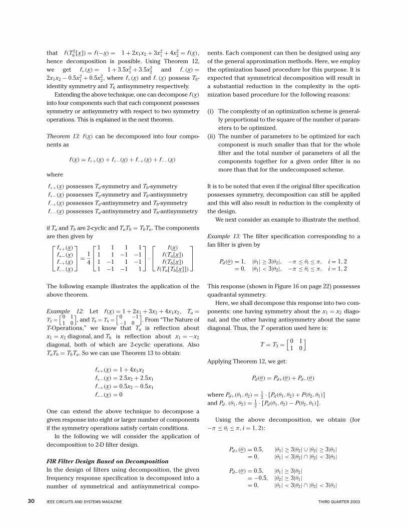
that f(T26 [x]) = f(−x) = 1 + 2x1x2 + 3x2

1 + 4x22 = f(x),

hence decomposition is possible. Using Theorem 12, we get f+(x) = 1 + 3.5x2

1 + 3.5x22 and f−(x) =

2x1x2 − 0.5x21 + 0.5x2

2 , where f+(x) and f−(x) possess T6-identity symmetry and T6 antisymmetry respectively.

Extending the above technique, one can decompose f(x)

into four components such that each component possessessymmetry or antisymmetry with respect to two symmetryoperations. This is explained in the next theorem.

Theorem 13: f(x) can be decomposed into four compo-nents as

f(x) = f++(x) + f+−(x) + f−+(x) + f−−(x)

where

f++(x) possesses Ta-symmetry and Tb-symmetryf+−(x) possesses Ta-symmetry and Tb-antisymmetryf−+(x) possesses Ta-antisymmetry and Tb-symmetryf−−(x) possesses Ta-antisymmetry and Tb-antisymmetry

if Ta and Tb are 2-cyclic and TaTb = TbTa. The componentsare then given by

f++(x)

f+−(x)

f−+(x)

f−−(x)

= 1

4

1 1 1 11 1 −1 −11 −1 1 −11 −1 −1 1

·

f(x)

f(Ta[x])f(Tb[x])

f(Ta[Tb[x]])

The following example illustrates the application of theabove theorem.

Example 12: Let f(x) = 1 + 2x1 + 3x2 + 4x1x2 , Ta =T3 =

[ 0 11 0

], and Tb = T4 =

[ 0 −1−1 0

]. From “The Nature of

T-Operations,” we know that Ta is reflection aboutx1 = x2 diagonal, and Tb is reflection about x1 = −x2

diagonal, both of which are 2-cyclic operations. AlsoTaTb = TbTa. So we can use Theorem 13 to obtain:

f++(x) = 1 + 4x1x2

f+−(x) = 2.5x2 + 2.5x1

f−+(x) = 0.5x2 − 0.5x1

f−−(x) = 0

One can extend the above technique to decompose agiven response into eight or larger number of componentsif the symmetry operations satisfy certain conditions.

In the following we will consider the application ofdecomposition to 2-D filter design.

FIR Filter Design Based on DecompositionIn the design of filters using decomposition, the givenfrequency response specification is decomposed into anumber of symmetrical and antisymmetrical compo-

nents. Each component can then be designed using anyof the general approximation methods. Here, we employthe optimization based procedure for this purpose. It isexpected that symmetrical decomposition will result ina substantial reduction in the complexity in the opti-mization based procedure for the following reasons:

(i) The complexity of an optimization scheme is general-ly proportional to the square of the number of param-eters to be optimized.

(ii) The number of parameters to be optimized for eachcomponent is much smaller than that for the wholefilter and the total number of parameters of all thecomponents together for a given order filter is nomore than that for the undecomposed scheme.

It is to be noted that even if the original filter specificationpossesses symmetry, decomposition can still be appliedand this will also result in reduction in the complexity ofthe design.

We next consider an example to illustrate the method.

Example 13: The filter specification corresponding to afan filter is given by

Pd(θ) = 1, |θ1| ≥ 3|θ2|, −π ≤ θi ≤ π, i = 1, 2= 0, |θ1| < 3|θ2|, −π ≤ θi ≤ π, i = 1, 2

This response (shown in Figure 16 on page 22) possessesquadrantal symmetry.

Here, we shall decompose this response into two com-ponents: one having symmetry about the x1 = x2 diago-nal, and the other having antisymmetry about the samediagonal. Thus, the T operation used here is:

T = T3 =[ 0 1

1 0

]

Applying Theorem 12, we get:

Pd(θ) = Pd+(θ) + Pd−(θ)

where Pd+(θ1, θ2) = 12 · [Pd(θ1, θ2) + P(θ2, θ1)]

and Pd−(θ1, θ2) = 12 · [Pd(θ1, θ2) − P(θ2, θ1)].

Using the above decomposition, we obtain (for−π ≤ θi ≤ π, i = 1, 2):

Pd+(θ) = 0.5, |θ1| ≥ 3|θ2| ∪ |θ2| ≥ 3|θ1|= 0, |θ1| < 3|θ2| ∩ |θ2| < 3|θ1|

Pd−(θ) = 0.5, |θ1| ≥ 3|θ2|= −0.5, |θ2| ≥ 3|θ1|= 0, |θ1| < 3|θ2| ∩ |θ2| < 3|θ1|


The responses of Pd+(θ) and Pd−(θ) are shown in Figures17 and 18, respectively, on pages 23 and 24. Pd+(θ) pos-sesses octagonal symmetry and Pd−(θ) possessesoctagonal antisymmetry. We next design these twocomponents using optimization.

For Pd+(θ), which has octagonal symmetry, we knowfrom Table 8 that akl = alk and bmn = 0. So assuming aimpulse response size of 5×5 for our filter, its frequencyresponse function will be:

P+(θ1, θ2) =2∑

k=0

2∑

l=0

akl · (cos θ1)k · (cos θ2)

l

with akl = alk.

Hence, there are 6 independent coefficients here. Thesecoefficients are determined by minimizing the objectivefunction:

J+ =∑∑

[P+(θ1, θ2) − Pd+(θ1, θ2)]2

The optimization required 129 function evaluations. Thefollowing are the optimized coefficients. The contour and3-D plots are shown in Figure 19 on page 25.

a00 = −0.07304

a01 = 0.1184

a02 = 0.4669

a10 = 0.1184

a11 = −0.2486

a12 = −0.02676

a20 = 0.4669

a21 = −0.02676

a22 = −0.5287

Next, we design the component, Pd−(θ), which pos-sesses octagonal antisymmetry of type 2 in Table 8. So,the frequency response function will be:

P−(θ1, θ2) =2∑

k=0

2∑

l=0

αkl · (cos θ1)k · (cos θ2)

l,

with αkl = −αlk and αkk = 0

Here there are 3 independent parameters, which aredetermined by minimizing the objective function

J− =∑∑

[P−(θ1, θ2) − Pd−(θ1, θ2)]2

The optimization required 60 function evaluations. Theoptimized parameters are given below and the resultingcontour and 3-D plots are shown in Figure 20 on page 28.

a00 = 0

a01 = 0.3612

a02 = 0.1949

a10 = −0.3612

a11 = 0

a12 = 0.09579

a20 = −0.1949

a21 = −0.09579

a22 = 0

The total frequency response function is obtained byadding P+(θ1, θ2) and P−(θ1, θ2), i.e.,

P(θ1, θ2) = P+(θ1, θ2) + P−(θ1, θ2)

The resulting contour and 3-D plots are given in Figure 21 on page 28.

So, by using decomposition, the design required129 + 60 = 189 function evaluations to determine a total of9 independent parameters. In comparison, the design with-out decomposition is found to require 246 function evalua-tions to determine 9 independent parameters. So theadvantage of using decomposition is clearly shown in theexample.

Conclusion

The objective of this paper is to present the variousresults available in the literature on the symmetries andtheir applications for two-dimensional signals and sys-tems. Specifically, a unified way of expressing the variouscommonly occurring symmetries is first presented andthen the interdependencies resulting from various sym-metries on signals and their Fourier transforms are devel-oped using the unified symmetry representation. Theapplication of symmetry conditions to speed up the fastFourier transform algorithms is then discussed. Analysisof the magnitude responses of filters shows that utiliza-tion of their symmetries will considerably simplify thecomplexity of the design and implementation of these fil-ters. Finally, techniques for the application of symmetryresults even for functions that do not possess symmetriesby using symmetrical decomposition are presented. Thevarious results and techniques presented in this papershow that a knowledge and application of the varioussymmetries in the responses of 2-D systems will consid-erably reduce the complexity of the design and imple-mentation of these systems. Symmetry with complexpolynomials will also provide similar advantage. Further,it may be noted that symmetry results can be extended tothree and higher dimensional systems [29, 30]. Althoughthe paper dealt with the symmetry in magnitude func-


tion, similar advantages can be obtained by identifyingphase symmetries. Due to lack of space these are not pre-sented in this paper. The more recent research in thesymmetry theory and its application to 2-D filter design isthrough the use of the delta operator. The main advan-tage with regard to the theory is that it unifies the resultsof 2-D analog and discrete-time case. From the point ofview of design, there is a major advantage in the coeffi-cient sensitivity for narrowband filters [31–36].

References[1] J. Rosen, Symmetry Discovered. Cambridge, England: Cambridge Uni-versity Press. 1975.[2] A.V. Shubinov and V.M. Koptsik, Symmetry in Science and Art. NewYork: Plenum Press. 1974.[3] A. Fettweis, “Symmetry requirements for multidimensional digital fil-ters,” Int. Journal Circuit Theory Appl., vol. 5, pp. 343–353, 1977.[4] M. Narasimha and A. Peterson, “On using symmetry of FIR filters fordigital interpolation,” IEEE Tran. Acoust., Speech, Signal Processing, vol.ASSP-26, pp. 267–268, 1978.[5] P. K. Rajan and M.N.S. Swamy, “Symmetry conditions on two-dimen-sional half-plane digital filter transfer functions,” IEEE Trans. Acoust.,Speech, Signal Processing, vol. ASSP-27, pp. 506–511, October 1979.[6] D.M. Goodman, “Symmetry Conditions for Two-dimensional FIR Fil-ters”, Lawerence Livermore Lab Rep. UCID-311, 1979.[7] S.A.H. Aly, J. Lodge and M.M. Fahmy, “The design of two-dimensionaldigital filters with symmetrical or anti-symmetrical specifications,” Proc.1980 Eur. Conf Circuit Theory Des., Warsaw, pp. 145–150, 1980.[8] D.M. Goodman, “Quadrantal symmetry calculations for nonsymmet-ric half-plane filters,” Proc. 14th Asilomar Conf, vol. 14, 1980.[9] S.A.H. Aly and M.M. Fahmy, “Symmetry exploitation in the design andimplementation of two-dimensional rectangularly sampled filters,” IEEETrans. Acoust., Speech, Signal Processing, vol. ASSP-29, pp. 973–982, 1981.[10] J.H. Lodge and M.M. Fahmy, “K-cyclic symmetries in multidimen-sional sampled signals,” IEEE Trans. Acoust., Speech, Signal Processing,vol. ASSP-31, pp. 847–860, 1983.[11] D.E. Dudgeon and R.M. Merserau, Multidimensional Digital SignalProcessing. Englewood Cliffs, NJ: Prentice-Hall, 1984.[12] B.P. George and A.N. Venetsanopoulos, “Design of two-dimensionalrecursive digital filters on the basis of quadrantal and octagonal sym-metry,” Circuits Syst. Signal Processing, vol. 3, pp. 59–78, 1984.[13] J. Pitas and A.N. Venetsanopoulos, “The use of symmetries in thedesign of multidimensional digital filters,” IEEE Trans. Circuits Syst., vol.CAS-33, pp. 863–873, 1986.[14] A. Fettweis, “Multidimensional digital filters with closed loss behav-ior designed by complex network theory approach,” IEEE Trans. CircuitsSyst., vol. CAS-34, pp. 338–344, 1987.[15] P.K. Rajan and M.N.S. Swamy, “Quadrantal symmetry associatedwith two-dimensional digital filter transfer functions”, IEEE Trans. Cir-cuits Syst., vol. CAS-25, pp. 340–343, June 1978.[16] P.K. Rajan, H.C. Reddy, and M.N.S. Swamy, “Further results on 4-foldrotational symmetry in 2-D functions”, Proc. 1982 IEEE Int. Conf. Acoust.,Speech, Signal Processing, Paris. May 1982.[17] P.K. Rajan, H.C. Reddy and M.N.S. Swamy, “Fourfold rotational sym-metry in two-dimensional functions”, IEEE Trans. Acoust., Speech, SignalProcessing. vol. ASSP-30, pp. 488–499, June 1982.[18] V. Rajaravivarma, P.K. Rajan and H.C. Reddy, “Symmetry study on 2-D complex analog and digital filter functions,” Multidimensional Sys-tems and Signal Processing, vol. 2, pp. 161–187, 1991.[19] M.N.S. Swamy and P.K. Rajan, “Symmetry in 2-D filters and its appli-cation,” in Multidimensional Systems: Techniques and Applications S.G.Tzafestas, Ed. New York: Marcel Dekker, 1986, Ch. 9.[20] H.C. Reddy, I.H. Khoo and P.K. Rajan, “Symmetry and 2-D FilterDesign”, The Circuits and Filters Handbook W. K. Chen, Ed. Boca Raton,FL: CRC Press, 2002.[21] H. Weyl, Symmetry. Princeton: Princeton University Press, 1952.[22] P.K. Rajan, H.C. Reddy, M.N.S. Swamy, “Symmetry relations in two-dimensional fourier transforms,” in Proc. 1984 IEEE-ISCAS, vol. 3, pp 1022–1025, 1984.

[23] G.A. Bliss, Algebraic Functions. New York: Dover, 1966.[24] P.K. Rajan, H.C. Reddy, “A test procedure for 2-D discrete scatteringHurwitz polynomials,” IEEE Transactions on Acoustics, Speech and SignalProcessing, vol. ASSP-37, pp. 118–120, January 1989.[25] H.C. Reddy, P.K. Rajan, “A comprehensive study of two-variableHurwitz polynomials,” IEEE-Trans. on Education, pp. 198–209, Aug. 1989.[26] H.C. Reddy, “Theory of two-timensional Hurwitz polynomials,” The Cir-cuits and Filters Handbook W. K. Chen, Ed. Boca Raton, FL: CRC Press, 2002.[27] P.K. Rajan and H.C. Reddy, “Symmetrical decomposition and Trans-formation,” Mathematics and Computers in Simulation, vol. 27, no 5/6, pp. 585–598, Oct. 1985.[28] V. Rajaravivarma, P.K. Rajan and H.C. Reddy, “Design of multidi-mensional FIR digital filters using symmetrical decomposition tech-nique,” IEEE Transactions on Signal Processing, vol. 42, no. 1, pp.164–174, Jan. ‘94.[29] V. Rajaravivarma, P.K. Rajan, H.C. Reddy, “Study of phase symmetryin 3-D filters,” Proc. Southeast Conference 1989, Columbia, South Carolina,April 1989.[30] V. Rajaravivarma, P.K. Rajan, H.C. Reddy, “Planar symmetries in 3-Dfilter responses and their application in 3-D filter design,” IEEE Transac-tions on Circuits and Systems II, vol. 39. no. 6, pp 356–368, June 1992.[31] H.C. Reddy, P.K. Rajan, G.S. Moschytz and A.R. Stubberud, “Study ofvarious symmetries in the frequency response of two-dimensional deltaoperator formulated discrete-time systems,” Proc. 1996 IEEE-ISCAS,vol. 2, pp. 344–347, May 1996. [32] H.C. Reddy, I.H. Khoo, G.S. Moschytz and A.R Stubberud, “Theoryand test procedure for symmetries in the frequency response of complextwo-dimensional delta operator formulated discrete-time systems,” Proc.the 1997 IEEE-ISCAS, vol. 4, pp. 2373–2376, June 1997. [33] H.C. Reddy, I.H. Khoo, P.K. Rajan, “Symmetry in the frequencyresponse of two-dimensional delta operator formulated discrete-timesystems,” Proc. the 1997 ECCTD, vol. 3, pp. 1118–1123, Aug 1997. [34] H.C. Reddy, I.H. Khoo, P.K. Rajan and A.R. Stubberud, “Symmetry inthe frequency response of two-dimensional (γ1, γ2) complex plane dis-crete-time systems,” Proc. 1998 IEEE-ISCAS, vol. 5, pp. 66–69, May 1998. [35] I.H. Khoo, H.C. Reddy and P.K. Rajan, “Delta operator based 2-D fil-ter design using symmetry constraints,” Proc. 2001 IEEE-ISCAS, vol. 2, pp781–784, May 2001. [36] I.H. Khoo, H.C. Reddy and P.K. Rajan, “Delta operator based 2-D fil-ters: Symmetry, stability, and design,” Proc. 2003 IEEE-ISCAS, May 2003.

Hari C. Reddy received the B.E. degreein electrical engineering in 1964 from SriVenkateswara University, Tirupati, India;the M.E. degree in electrical engineeringfrom M.S. University of Baroda, Baroda,India in 1966; and the Ph.D. degree inelectronics and communication engi-

neering, from Osmania University, Hyderabad, India in1974. He then did two years of post doctoral researchwork at the Concordia University, Montreal, Canada,1975–1977.

Professor Reddy has been with the Department ofElectrical Engineering, California State University, LongBeach (CSULB), as a tenured professor since 1987. Dr.Reddy was with the Department of Electrical Engineer-ing at Tennessee Technological University, Cookeville,Tennessee associate professor from 1980–1983 and astenured professor from 1983–1987. Before joining Ten-nessee Tech, Dr. Reddy held teaching and research posi-tions at the State University of New York College atBuffalo; Concordia University, Montreal, Canada; Osma-


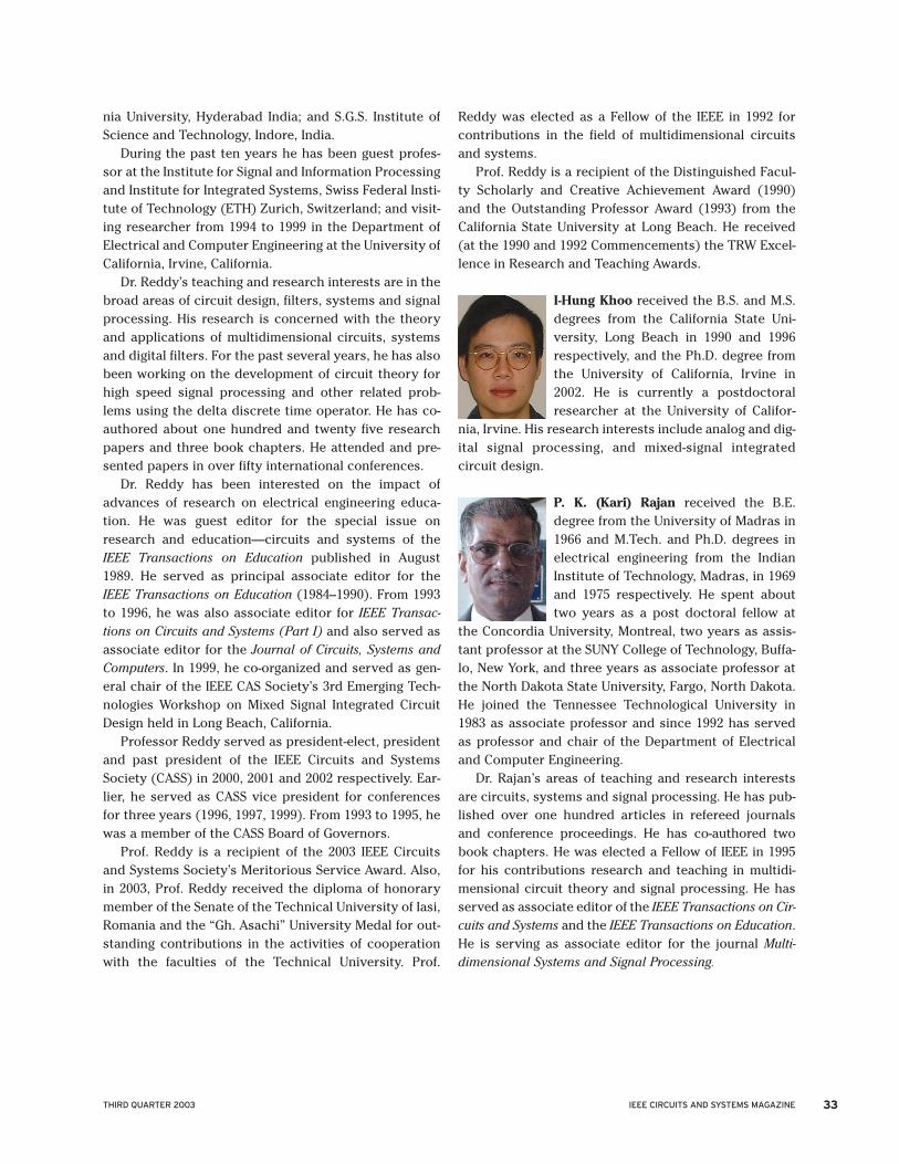
nia University, Hyderabad India; and S.G.S. Institute ofScience and Technology, Indore, India.

During the past ten years he has been guest profes-sor at the Institute for Signal and Information Processingand Institute for Integrated Systems, Swiss Federal Insti-tute of Technology (ETH) Zurich, Switzerland; and visit-ing researcher from 1994 to 1999 in the Department ofElectrical and Computer Engineering at the University ofCalifornia, Irvine, California.

Dr. Reddy’s teaching and research interests are in thebroad areas of circuit design, filters, systems and signalprocessing. His research is concerned with the theoryand applications of multidimensional circuits, systemsand digital filters. For the past several years, he has alsobeen working on the development of circuit theory forhigh speed signal processing and other related prob-lems using the delta discrete time operator. He has co-authored about one hundred and twenty five researchpapers and three book chapters. He attended and pre-sented papers in over fifty international conferences.

Dr. Reddy has been interested on the impact ofadvances of research on electrical engineering educa-tion. He was guest editor for the special issue onresearch and education—circuits and systems of theIEEE Transactions on Education published in August1989. He served as principal associate editor for theIEEE Transactions on Education (1984–1990). From 1993to 1996, he was also associate editor for IEEE Transac-tions on Circuits and Systems (Part I) and also served asassociate editor for the Journal of Circuits, Systems andComputers. In 1999, he co-organized and served as gen-eral chair of the IEEE CAS Society’s 3rd Emerging Tech-nologies Workshop on Mixed Signal Integrated CircuitDesign held in Long Beach, California.

Professor Reddy served as president-elect, presidentand past president of the IEEE Circuits and SystemsSociety (CASS) in 2000, 2001 and 2002 respectively. Ear-lier, he served as CASS vice president for conferencesfor three years (1996, 1997, 1999). From 1993 to 1995, hewas a member of the CASS Board of Governors.

Prof. Reddy is a recipient of the 2003 IEEE Circuitsand Systems Society’s Meritorious Service Award. Also,in 2003, Prof. Reddy received the diploma of honorarymember of the Senate of the Technical University of Iasi,Romania and the “Gh. Asachi” University Medal for out-standing contributions in the activities of cooperationwith the faculties of the Technical University. Prof.

Reddy was elected as a Fellow of the IEEE in 1992 forcontributions in the field of multidimensional circuitsand systems.

Prof. Reddy is a recipient of the Distinguished Facul-ty Scholarly and Creative Achievement Award (1990)and the Outstanding Professor Award (1993) from theCalifornia State University at Long Beach. He received(at the 1990 and 1992 Commencements) the TRW Excel-lence in Research and Teaching Awards.

I-Hung Khoo received the B.S. and M.S.degrees from the California State Uni-versity, Long Beach in 1990 and 1996respectively, and the Ph.D. degree fromthe University of California, Irvine in2002. He is currently a postdoctoralresearcher at the University of Califor-

nia, Irvine. His research interests include analog and dig-ital signal processing, and mixed-signal integratedcircuit design.

P. K. (Kari) Rajan received the B.E.degree from the University of Madras in1966 and M.Tech. and Ph.D. degrees inelectrical engineering from the IndianInstitute of Technology, Madras, in 1969and 1975 respectively. He spent abouttwo years as a post doctoral fellow at

the Concordia University, Montreal, two years as assis-tant professor at the SUNY College of Technology, Buffa-lo, New York, and three years as associate professor atthe North Dakota State University, Fargo, North Dakota.He joined the Tennessee Technological University in1983 as associate professor and since 1992 has servedas professor and chair of the Department of Electricaland Computer Engineering.

Dr. Rajan’s areas of teaching and research interestsare circuits, systems and signal processing. He has pub-lished over one hundred articles in refereed journalsand conference proceedings. He has co-authored twobook chapters. He was elected a Fellow of IEEE in 1995for his contributions research and teaching in multidi-mensional circuit theory and signal processing. He hasserved as associate editor of the IEEE Transactions on Cir-cuits and Systems and the IEEE Transactions on Education.He is serving as associate editor for the journal Multi-dimensional Systems and Signal Processing.


2-d symmetry: theory and filter design applications - circuits and

Documents