2. a theory of current account determination - holger · pdf filechapter 2. a theory of...

Chapter 2. A Theory of Current Account Determination

2. A Theory of Current Account Determination

Small Open Economy

Decisions at home don’t affect world prices and interest rates (r = r∗)

2 periods; goods can’t be stored; households consume or save by buyingbonds

Endowment economy: production (GDP) Q is given (as well as initial NIIP)

Period 1 budget constraint: C1 + B∗1 − B∗

0 = r0B∗0 + Q1

Period 2 budget constraint: C2 + B∗2 − B∗

1 = r1B∗1 + Q2

Combining the budget constraints and noting B∗2 = 0: life time budget constraint

C1 +C2

1 + r1= (1 + r0)B∗

0 + Q1 +Q2

1 + r1(1)

Professor Dr. Holger Strulik Open Economy Macro 1 / 31


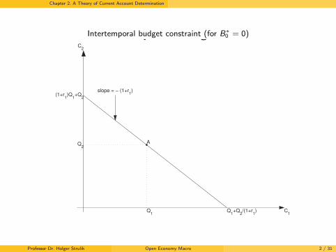
Intertemporal budget constraint (for B∗0 = 0)The intertemporal budget constraint

Q1+Q

2/(1+r

1)

(1+r1)Q

1+Q

2

C1

C2

slope = − (1+r1)

A

Q1

Q2



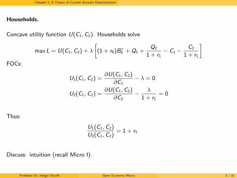
Households.

Concave utility function U(C1,C2). Households solve

max L = U(C1,C2) + λ

[(1 + r0)B∗

0 + Q1 +Q2

1 + r1− C1 −

C2

1 + r1

]FOCs:

U1(C1,C2) =∂U(C1,C2)

∂C1− λ = 0

U2(C1,C2) =∂U(C1,C2)

∂C2− λ

1 + r1= 0

Thus:

U1(C1,C2)

U2(C1,C2)= 1 + r1

Discuss: intuition (recall Micro I).



Equilibrium.

Suppose identical individuals

individual variables are interpreted as country aggregates

thus no borrowing within economies; individual budget constraint is the economy’sresource constraint

B∗t is net foreign asset position (world market interest rate r∗)

Equilibrium is a consumption bundle (C1,C2) that satisfies

C1 +C2

1 + r1= (1 + r0)B∗

0 + Q1 +Q2

1 + r1U1(C1,C2)

U2(C1,C2)= 1 + r1

r = r∗

given the exogenous variables {r0,B∗0 ,Q1,Q2, r

∗}.



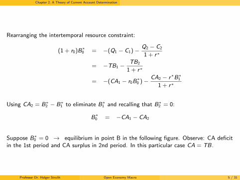
Rearranging the intertemporal resource constraint:

(1 + r0)B∗0 = −(Q1 − C1)− Q2 − C2

1 + r∗

= −TB1 −TB2

1 + r∗

= −(CA1 − r0B∗0 )− CA2 − r∗B∗

1

1 + r∗

Using CA2 = B∗2 − B∗

1 to eliminate B∗1 and recalling that B∗

2 = 0:

B∗0 = −CA1 − CA2

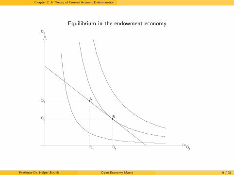
Suppose B∗0 = 0 → equilibrium in point B in the following figure. Observe: CA deficit

in the 1st period and CA surplus in 2nd period. In this particular case CA = TB.



Equilibrium in the endowment economy

C1

C2

A

Q1

Q2

B

C1

C2



How do shocks affect the CA?

Consider negative income shock:

Temporary shock only in period 1 (or only period 2)

Permanent shock, i.e. here in both periods

Notice: in period 1 the shock is observed, in period 2 it is expected

Response of CA will depend largely on the nature of the shock...



1. Temporary income shock in period 1

Budget constraint after a temporary negative output shock in period 1

C1

C2

A

Q1

Q2

A′

Q1−∆



Equilibrium after a temporary negative output shock in period 1

C1

C2

A

Q1

Q2

A′

Q1−∆

B

C1

C2

B′

C1

′

C2

′

Observe: Larger trade deficit in period 1 and larger surplus in period 2 due toconsumption smoothing. Adjustment runs via the CA.



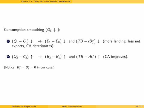
Consumption smoothing (Q1 ↓ ):

1 (Q1 − C1) ↓ → (B1 − B0) ↓ and (TB − rB∗0 ) ↓ (more lending, less net

exports, CA deteriorates)

2 (Q2 − C2) ↑ → (B2 − B1) ↑ and (TB − rB∗1 ) ↑ (CA improves).

(Notice: B∗0 = B∗

2 = 0 in our case.)



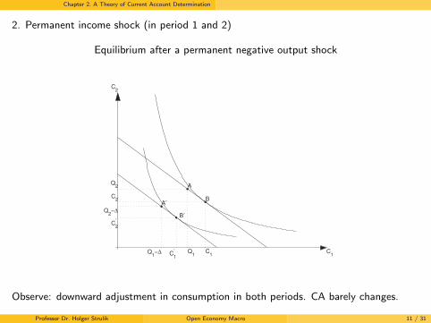
2. Permanent income shock (in period 1 and 2)

Equilibrium after a permanent negative output shock

C1

C2

A

Q1

Q2

A′

Q1−∆

Q2−∆

B

C1

C2

B′

C1

′

C2

′

Observe: downward adjustment in consumption in both periods. CA barely changes.



General principle:

adjust to temporary output shocks by running CA deficits or surpluses

adjust to permanent output shocks by changing spending

But then: how did global imbalances accumulate?



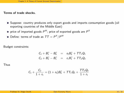
Terms of trade shocks.

Suppose: country produces only export goods and imports consumption goods (oilexporting countries of the Middle East)

price of imported goods PM ; price of exported goods are PX

Define: terms of trade as TT = PX/PM

Budget constraints:

C1 + B∗1 − B∗

0 = r0B∗0 + TT1Q1

C2 + B∗2 − B∗

1 = r1B∗1 + TT2Q2

Thus

C1 +C2

1 + r1= (1 + r0)B∗

0 + TT1Q1 +TT2Q2

1 + r1



Observe:

TT shocks work like shocks to output

Temporary negative TT shock → CA decreases and consumption smoothing

Permanent negative TT shock → permanent decrease in consumption, CA barelychanges.

The Role of Expectations:Does observation of

little change of CA after a temporary shock

large change of CA after a permanent shock

contradict the theory?

→ not necessarily, if individuals predicted the nature of the shock wrongly.



World interest rate shock (r∗ ↑ )

Observe:

Substitution effect and income effect

Suppose: substitution effect dominates (savings increase)

C1

C2

Y1 C1

C2

Y2

Adjustment to a world interest rate shock

B

B′

A

C1′

C2′

slope = −(1 + r′ + ∆)



Example Log-Utility.

U(C1,C2) = logC1 + logC2

Define discounted total wealth of households Q̄ = (1 + r0)B∗0 + Q1 + Q2

1+r∗

From Log-utility

U1(C1,C2) =1

C1U2(C1,C2) =

1

C2

Budget constraint:

Q̄ − C1 −C2

1 + r∗= 0

Implied FOC:

1

C1= (1 + r∗)

1

C2.

Thus from FOC and budget constraint:

C1 =1

2Q̄.



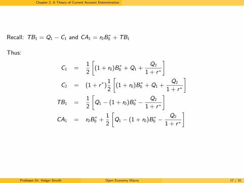
Recall: TB1 = Q1 − C1 and CA1 = r0B∗0 + TB1

Thus:

C1 =1

2

[(1 + r0)B∗

0 + Q1 +Q2

1 + r∗

]C2 = (1 + r∗)

1

2

[(1 + r0)B∗

0 + Q1 +Q2

1 + r∗

]TB1 =

1

2

[Q1 − (1 + r0)B∗

0 −Q2

1 + r∗

]CA1 = r0B

∗0 +

1

2

[Q1 − (1 + r0)B∗

0 −Q2

1 + r∗

]



Observe (by taken derivatives):

Temporary output shock: If Q1 falls by one unit, TB1 and CA1 decrease by 1/2 dueto consumption smoothing

Permanent shock: If both Q1 and Q2 fall by one unit then TB1 and CA1 decline byr∗/(2 + 2r∗), i.e. only little for moderate r∗.

For increase in the world interest rate r∗ we see that C1 falls such that CA1 andTB1 improve

The latter effect is independent of B∗0 (whether the country is a debtor or a

creditor).

Discuss: why?



Capital controls.

Assume: government wants to reduce the CA deficit and imposes capital controls

e.g. taxes on capital imports

here drastic control: prohibition of international foreign borrowing

Only consumption at the endowment point

Thus C1 = Q1 and C2 = Q2 such that CA1 = 0 and TB1 = 0

Optimality condition

U1(Q1,Q2)

U2(Q1,Q2)= 1 + r1

with one unknown endogenous variable r1.

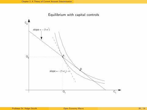
Observe:

r1 > r∗

the smaller Q1/Q2 the higher r1

capital controls make households unhappy (in the short-run)



Equilibrium with capital controls

slope = − (1+r1) →

C1

C2

A

Q1

Q2

B

slope = − (1+r*)



Uncertainty and the Current Account.

During Great Moderation output volatility decreased

3 possible explanations:

I good luck (no big wars, no oil price crises,...)I good monetary policy (Greenspan and the Taylor-Rule)I structural change (less manufacturing, more IT, and less need for inventory

management; financial innovations(?) )

At the same time the CA deteriorated in the US

Is there a connection?



(a) Real Per Capita U.S. GDP Growth 1947Q2-2015Q4

1950 1960 1970 1980 1990 2000 2010−3

−2

−1

0

1

2

3

4

Year

100×ln

(

yt

yt−

1

)

← 1984

std

(

lnytyt−1

)

= 0.012 std

(

lnytyt−1

)

= 0.006



(b) U.S. Current Account to GDP Ratio 1947Q1-2015Q4

1950 1960 1970 1980 1990 2000 2010−7

−6

−5

−4

−3

−2

−1

0

1

2

3

4

Year

100×

(

cat

yt

)

← 1984

mean

(

catyt

)

= 0.004 mean

(

catyt

)

= -0.03



Model with Uncertainty

Idea:

Precautionary savings motive

Great Moderation → lower uncertainty (lower std.dev. of output σ). Does it leadto a deteriorating CA?

Reference Situation: Certainty

Q1 = Q2 = Q

U = logC1 + logC2

B∗0 = 0

r∗ = 0

Max logC1 + log(2Q − C1). FOC:

1/C1 = 1/(2Q − C1) ⇒ C1 = Q = C2

Thus CA1 = Q1 − C1 = 0. No int. borrowing/lending.



New Situation: Q2 is uncertain.

Let Q1 = Q and

Q2 =

{Q + σ with probability 1/2

Q − σ with probability 1/2

Notice: σ is the standard deviation of Q2 ( → why?)

Expected utility function: U(C1,C2) = logC1 + E logC2

Budget constraints:

C2 = 2Q + σ − C1 in the good state

C2 = 2Q − σ − C1 in the bad state

Implied expected lifetime utility:

logC1 +1

2log(2Q + σ − C1) +

1

2log(2Q − σ − C1).



FOC:1

C1=

1

2

[1

2Q + σ − C1+

1

2Q − σ − C1

]Households equate marginal utility of period 1 consumption to expected marginal utilityof period 2 consumption

Is the certainty solution (C1 = C2 = Q) optimal? This would imply

1

Q=

1

2

[1

Q + σ+

1

Q − σ

]⇒ 1 =

Q2

Q2 − σ2

→ only for σ = 0; impossible for σ > 0.



Observe:

LHS < RHS of the FOC (verify that ∂RHS/∂σ > 0)

Thus households can increase utility by lowering C1 (below Q)

The larger uncertainty is (the higher σ), the smaller C1

This is precautionary saving

It leads to a TB surplus

Intuition:

concave utility function (convex marginal utility)

σ units of extra consumption increase utility less that σ units less consumptionreduce utility...



A

Q

1

Q

B

Q− σ

C

Q+ σ

D1

2

1

Q− σ+

1

2

1

Q+σ

C1

← 1/C1

Note. The solid line plots the marginal utility of consumption in period

1, 1/C1. In the case that C1 = Q, point D indicates the expected

marginal utility of consumption in period 2 and point A indicates the

marginal utility of consumption in period 1.



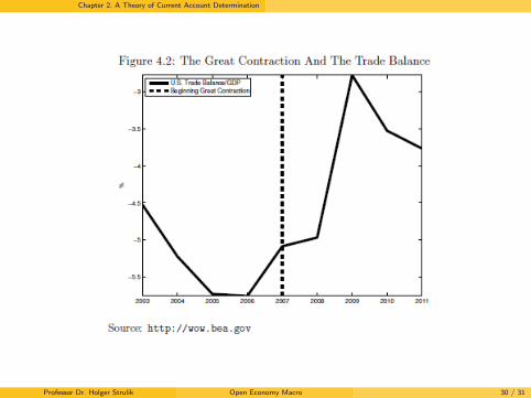
Great Moderation: σ ↓ . Model predicts deterioration of TB.

A test of the model would be to assess it for the current economic andfinancial crisis

σ increased in the US after 2007

The model would predict an improvement of the trade balance.

This is what happened. The trade balance improved by around 2%age points.



Discuss:

Can the great moderation really motivate permanent TB deficits?

great moderation → overconfidence → the great recession?

Robert Lucas (2003): “The central problem of depression-prevention has beensolved, for all practical purposes.”


2. a theory of current account determination - holger · pdf filechapter 2. a theory of...

Documents