2-2-11

2-2-22

Chapter Two

Descriptive Statistics

McGraw-Hill/Irwin Copyright © 2004 by The McGraw-Hill Companies, Inc. All rights reserved.

2-2-33

Descriptive Statistics

2.1 Describing the Shape of a Distribution

2.2 Describing Central Tendency

2.3 Measures of Variation

2.4 Percentiles, Quartiles, and Box-and-Whiskers Displays

2.5 Describing Qualitative Data

*2.6 Using Scatter Plots to Study the Relationship Between Variables

*2.7 Misleading Graphs and Charts

2-2-44

2.1 Stem and Leaf Display: Car Mileage

Example 2.1: The Car Mileage Case

1 29 8 5 30 1344 12 30 5666889 21 31 001233444 (11) 31 55566777889 17 32 0001122344 7 32 556788 1 33 3

2-2-55

Stem and Leaf Display: Payment Times

Example 2.2: The Accounts Receivable Case

1 10 0 2 11 0 4 12 00 7 13 000 11 14 0000 18 15 0000000 27 16 000000000 (8) 17 00000000 30 18 000000 24 19 00000 19 20 000 16 21 000 13 22 000 10 23 00 8 24 000 5 25 00 3 26 0 2 27 0 1 28 1 29 0

2-2-66

Histograms

Example 2.4: The Accounts Receivable Case

Frequency Histogram Relative Frequency Histogram

2-2-77

The Normal Curve

2-2-88

Skewness

Right SkewedLeft Skewed Symmetric

2-2-99

Dot Plots

Scores on Exams 1 and 2Scores on Exams 1 and 2

2-2-1010

2.2 Population Parameters and Sample Statistics

A population parameter is number calculated from all the population measurements that describes some aspect of the population.

The population mean, denoted , is a population parameter and is the average of the population measurements.

A point estimate is a one-number estimate of the value of a population parameter.

A sample statistic is number calculated using sample measurements that describes some aspect of the sample.

2-2-1111

Measures of Central Tendency

Mean, σ The average or expected value

Median, Md The middle point of the ordered measurements

Mode, Mo The most frequent value

2-2-1212

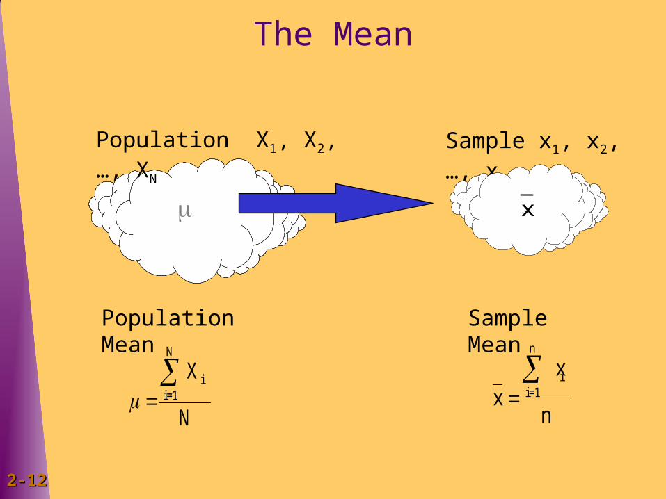
The Mean

Population X1, X2, …, XN

Population Mean

N

X

N

1=ii

Sample x1, x2, …, xn

Sample Mean

n

xx

n

1=ii

x

2-2-1313

The Sample Mean

The sample mean is defined asx

n

xxx

n

xx n

n

ii

...211

and is a point estimate of the population mean, .

2-2-1414

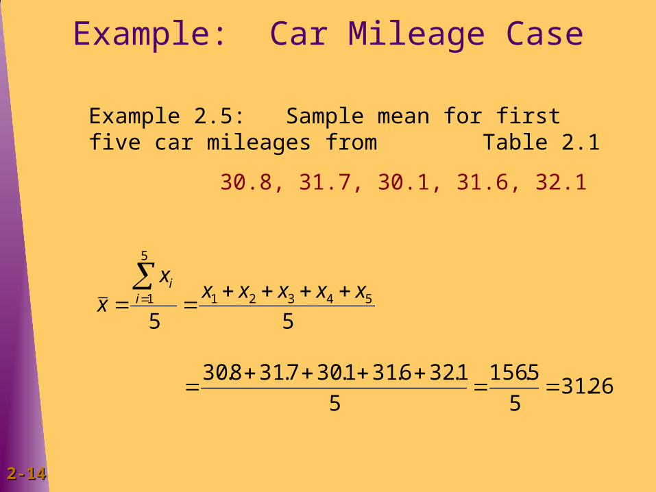
Example: Car Mileage Case

Example 2.5: Sample mean for first five car mileages from Table 2.1

30.8, 31.7, 30.1, 31.6, 32.1

26.315

5.156

5

1.326.311.307.318.30

5554321

5

1 xxxxxx

x ii

2-2-1515

The Median

The population or sample median is a value such that 50% of all measurements lie above (or below) it.

The median Md is found as follows:

1. If the number of measurements is odd, the median is the middlemost measurement in the ordered values.

2. If the number of measurements is even, the median is the average of the two middlemost measurements in the ordered values.

2-2-1616

Example: Sample Median

Example 2.6: Internists’ Salaries (x$1000)

127 132 138 141 144 146 152 154 165 171 177 192 241

Since n = 13 (odd,) then the median is the middlemost or 7th measurement, Md=152

2-2-1717

The Mode

The mode, Mo of a population or sample of measurements is the measurement that occurs most frequently.

2-2-1818

Example: Sample Mode

Example 2.2: The Accounts Receivable Case

1 10 0 2 11 0 4 12 00 7 13 000 11 14 0000 18 15 0000000 27 16 000000000 (8) 17 00000000 30 18 000000 24 19 00000 19 20 000 16 21 000 13 22 000 10 23 00 8 24 000 5 25 00 3 26 0 2 27 0 1 28 1 29 0

The value 16 occurs 9 times therefore:

Mo = 16

2-2-1919

Relationships Among Mean, Median and Mode

2-2-2020

2.3 Measures of Variation

Range

Largest minus the smallest measurement

Variance

The average of the sum of the squared deviations from the mean

Standard Deviation

The square root of the variance

2-2-2121

The Range

Example:

Internists’ Salaries (in thousands of dollars)

127 132 138 141 144 146 152 154 165 171 177 192 241

Range = 241 - 127 = 114 ($114,000)

Range = largest measurement - smallest measurement

2-2-2222

The Variance

Population X1, X2, …, XN

Population Variance

(X - )

N2

i2

i=1

N

σ2

Sample x1, x2, …, xn

Sample Variance

1-n

)x - (x =s

n

1=i

2i

2

s2

2-2-2323

The Standard Deviation

Population Standard Deviation, s: 2

Sample Standard Deviation, s:2ss

2-2-2424

Example: Population Variance/Standard Deviation

Population of annual returns for five junk bond mutual funds:

10.0%, 9.4%, 9.1%, 8.3%, 7.8%

m= 10.0+9.4+9.1+8.3+7.8 = 44.6 = 8.92%

5 50

22 2 2 2 210 0 8 92 9 4 8 92 91 8 92 8 3 8 92 7 8 8 92

5

( . . ) ( . . ) ( . . ) ( . . ) ( . . )

= 1.1664+.2304+.3844+1.2544 = 3.068 = .6136 5 5

2 6136 7833. .

2-2-2525

Example: Sample Variance/Standard Deviation

26.31 x

4

)26.311.32()26.316.31()26.311.30()26.317.31()26.318.30(=s

222222

s2 = 2.572 4 = 0.643

8019.0643.2 ss

Example 2.11: Sample variance and standard deviation for first five car mileages from Table 2.1

30.8, 31.7, 30.1, 31.6, 32.1

1-5

)x - (x =s

5

1=i

2i

2

2-2-2626

The Empirical Rule for Normal Populations

If a population has mean m and standard deviation s and is described by a normal curve, then

68.26% of the population measurements lie within one standard deviation of the mean: [m-s, m+s]

95.44% of the population measurements lie within two standard deviations of the mean: [m-2s, m+2s]

99.73% of the population measurements lie within three standard deviations of the mean: [m-3s, m+3s]

2-2-2727

Example: The Empirical Rule

Example 2.13: The Car Mileage Case

2-2-2828

Chebyshev’s Theorem

Let m and s be a population’s mean and standard deviation, then for any value k>1,

At least 100(1 - 1/k2 )% of the population measurements lie in the interval:

[m-ks, m+ks]

2-2-2929

2.4 Percentiles and Quartiles

For a set of measurements arranged in increasing order, the pth percentile is a value such that p percent of the measurements fall at or below the value and (100-p) percent of the measurements fall at or above the value.

The first quartile Q1 is the 25th percentile

The second quartile (or median) Md is the 50th percentile

The third quartile Q3 is the 75th percentile.

The interquartile range IQR is Q3 - Q1

2-2-3030

Example: Quartiles

20 customer satisfaction ratings:

1 3 5 5 7 8 8 8 8 8 8 9 9 9 9 9 10 10 10 10

Md = (8+8)/2 = 8

Q1 = (7+8)/2 = 7.5 Q3 = (9+9)/2 = 9

IRQ = Q3 - Q1 = 9 - 7.5 = 1.5

2-2-3131

Box and Whiskers Plots

2-2-3232

2.5 Describing Qualitative Data

2-2-3333

Population and Sample Proportions

Population X1, X2, …, XN

p

Population Proportion

Sample x1, x2, …, xn

Sample Proportion

n

xˆ

n

1=ii

p

p̂

xi = 1 if characteristic present, 0 if not

2-2-3434

Example: Sample Proportion

Example 2.16: Marketing Ethics Case

117 out of 205 marketing researchers disapproved of action taken in a hypothetical scenario

X = 117, number of researches who disapprove

n = 205, number of researchers surveyed

Sample Proportion: 117

p .57n 205

X

2-2-3535

Bar Chart

Percentage of Automobiles Sold by Manufacturer,1970 versus 1997

2-2-3636

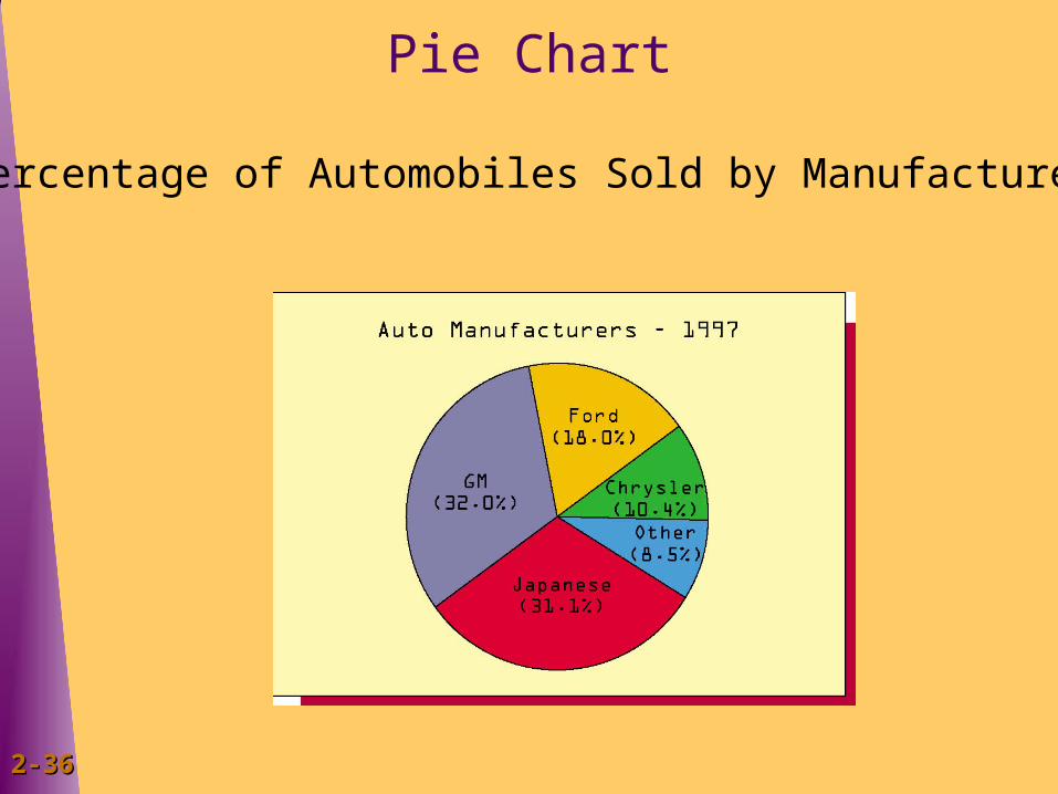
Pie Chart

Percentage of Automobiles Sold by Manufacturer,1997

2-2-3737

Pareto Chart

Pareto Chart of Labeling Defects

2-2-3838

2.6 Scatter Plots

Restaurant Ratings: Mean Preference vs. Mean Taste

2-2-3939

2.7 Misleading Graphs and Charts: Scale Break

Mean Salaries at a Major University, 1999 - 2002

2-2-4040

Misleading Graphs and Charts:Horizontal Scale Effects

Mean Salary Increases at a Major University, 1999-2002

2-2-4141

Descriptive Statistics

2.1 Describing the Shape of a Distribution

2.2 Describing Central Tendency

2.3 Measures of Variation

2.4 Percentiles, Quartiles, and Box-and-Whiskers Displays

2.5 Describing Qualitative Data

*2.6 Using Scatter Plots to Study the Relationship Between Variables

*2.7 Misleading Graphs and Charts

Summary: