1VFOR-TR- 82-0367 TR-312

STUDY OF TURBULENT BOUNDARY LAYERS OVER ROUGHSURFACES, WITH EMPHASIS ON THE EFFECTS OF

ROUGHNESS CHARACTER AND MACH NUMBER

4Pto Report

by

X. L. Finson

February 1982

Sponsored by

Air Force Office of Scientific Research (AFSC)United States Air Force

Under Contract No. F49620-80-C-0015

PHYSICAL SCIENCES INC.30 COMMERCE WAY, WOBURN, MASS. 01801

82 05 05 018hppwove6 for puble U10a.oMOdistributitol ... * d

The views and conclusions contained in this document are those of theauthors and should not be interpreted as necessarily representing the officialpolicies or endorsements, either expressed or impled, of the Air Force Officeof Scientific Research of the U. S. Government.

TR-312

STUDY OF TURBULENT BOUNDARY LAYERS OVER ROUGHSURFACES, WITH EMPHASIS ON THE EFFECTS OF

ROUGHNESS CHARACTER AND MACH NUMBER

-- T/ Report

by

j M. L. Finson

February 1982

Sponsored by

Air Force Office of Scientific Research (AFSC)United States Air Force

.0

Under Contract No. F49620-80-C-0015 n

. . ..F" .... ...

Al 7tro-7 C7

npprc,

MATTHEW J.Chief, Teclnical Iformation Division

" iiiii r ~~~~...- . . r,.. . . . .

3 ACKNOWLEDGEMENT

This research was sponsored by the Air Force Office of Scientific Re-search (AFSC), United States Air Force, under Contract #P49620-80-C-0015. The3 United States Gnvernment is authorized to reproduce and distribute reprintsfor governmental purposes notwithstanding any copyright notation hereon.

IoTU R

ITC RI.1nopoIutfcairn

ITG b

* *I~::II~i~ Avat)SbilitY C0648I Avbjl and/orDie Spc"

W;.

UNCLASSIFIEDSECURITY CLASSIFICATION OF T0415 PAGE (Wh"oe. &*.two*M

REPORT DOCUMENTATION PAGE B 3ADI COhI;ETING PQ

AFOSR-TR- 8 2 03 6 rJIJ4. TIT LE (OW Ss&MUI.) 0. MYEO RPR & PERGO CoVERED

Study of Turbulent Boundary Layers over Rough INTERIM (ANNUAL)Surfaces, with Emphasis on the Effects of 1 NOV 80 - 30 SEP 81Roughness Character and Mach Numb~er 6. Pe~rORMIN ORG. R&PORT NUMBER.

AUTNR(.)S. -CONTRACT oRt CRn&T "U"WPive

M. L. Finson F49620-80C0015

ZMAFIRMING CRANIZ'44ION NAME AND ADDRESS 10. PPOGRAM EtLFMCUT. PROJECT. TASKAREA & WORK %OITS ONUNRERS

PHYSICAL SCIEIACES INC.30 Commerce WA761102FWoburn, MA olsrbi 2307/AlCONTROLLING OFFICE NAME AND ADDRESS 12. REPORT OAT6

Air Force Office of Scientific Research/NA February 1982

Boiling AFB, D.C. 20332 1"7NUMBER OF PAGES

rrMONITtPRING AGENCY NAME 11 AODRIESS(If Olifewovs hef CosnbWflbm 0Mg.e) - I. SECURITY CLASS. .- 1 040 #VEWof)

Unclass ified

III& DECLASS Pica ri~n/ miH(rsaetcIUG

SCHEDULE

10 DISTRIBUTION STATEMENT fofli. Repot)l

Approved for public release; distribution unlimited.

17. DISTRIBUTION STATEMENT (of Ihe ahefrogI mInioi Urn Block20 If ~ltero bou Ro..t)

IS. SUPPLEMENTARY NOTES

Is. Key WORDS (Ceone an "ve@ide It neeS0aeww miden~ify 6? blok tMS r

Turbulent Boundary LayersTurbulent Heat TransferRe-entry Heating

20. ASISTMACT (Conu.Ida roR w DW siade it necess~ar o nU to by week sbc

A Reynolds stress model for turbulent boundary layers on roughwalls is used to investigate the effects of roughness character andcompressibility. The flow around roughness elements is treated asform drag. A method is presented for deriving the required roughnessshape and spacing from profilometer surface measurements. Calculationsbased on the model ccmnpare satisfactorily with low speed data onroughness character and hypersonic measurements with grit roughness

DD I jA 7 1473 90DIotIO or INov 05 is OmsoLcT

SECURITY CL;AMIIATIN P hIS atE60Sa.3o

UNCLASSIFIEDmuaabuyy CL MSPicAVWU OF "MS PAuMm be" ,

'' "

The computer model is exercised systematically over a wide range ofparameters to derive a practical scaling law for the equivalent rough-ness. In contrast to previous correlations, for most roughnesselement shapes the effective roughness is not predicted to show apronounced maximum as the element spacing decreases. The effect ofroughness tends to be reduced with increasing edge Mach number, primarilydue to decreasing density in the vicinity of the roughness elements.It is further shown that the required roughness Reynolds number for fullyrough behavior increases with increasing Mach number, explaining thesmall roughness effects observed in some hypersonic tests.

UNCLASSIFIED

ms~y hamNSY--i

I

ABSTRACT

A Reynolds stress model for turbulent boundary layers on rough walls

I is used to investigate the effects of roughness character and compressibility.

The flow around roughness elements is treated as form drag. A method is pre-

I sented for deriving the required roughness shape and spacing from profilometer

surface measurements. Calculations based on the model compare satisfactorily

with low speed data on roughness character and hypersonic measurements with

grit roughness. The computer model is exercised systematically over a wide

range of parameters to derive a practical scaling law for the equivalent

I roughness. In contrast to previous correlations, for most roughness element

shapes the effective roughness is not predicted to show a pronounced maximum

Ias the element spacing decreases. The effect of roughness tends to be reduced

with increasing edge Mach number, primarily due to decreasing density in the

I vicinity of the roughness elements. It is further shown that the required

roughness Reynolds number for fully rough behavior increases with increasing

Mach number, explaining the small roughness effects observed in some hyperson-

ic tests.

I

IIII

I

iI I

~~~~~~~~~~. .. ... . . . . . . . . . . . . ..... ;. '.... ... . ' , - ,......... ... .. . ..... ... . .

W

I TABLE OF CONTENTS

Section Page

Abstract i

1. Introduction I

2. Rough Wall Boundary Layer Model 9

3. Specification of Roughness Characteristics 13

1 4. Comparisons with Roughness Character Data 16

5. Comparisons with Compressible Roughness Data 24

1 6. Roughness Scaling Law 37

6.1 Incompressible Fully-Rough Flow 396.2 Compressible Flows-Fully Rough 486.3 Rough/Smooth Transition 546.4 Rough Wall Prandtl Number 57

I List of Symbols 61

11I111

1 -iii-

1ILIST OF FIGURES

Figure Page

1. Simpson's correlation for the effect of roughnessdensity. 6

2. Sketch of typical profilometer trace. 14

1 3. Comparison of present model with Schlichting's measure-ments for spherical roughness as a function of spacing. 17

4. Comparison of present model with Schlichting's measure-ments for spherical segment roughness as a function ofspacing. 18

1 5. Comparison of present model with Schlichting's measure-ments for conical roughness as a function of spacing. 19

6, Comparison of present model with Schlichting's measure-ments for short angle roughness as a function of spacing. 20

1 7. Comparison of present model with the measurements of.Raupach, Thom and Edwards for cylindrical roughnesselements at various spacings. 21

1 8. Comparison of present model with the measurements ofMiragaoker and Charlu on stones at various spacings. 22

1 9. Average roughness elements for Holden's "4 mil"roughness, for two methods of application. 25

1 10. Comparison of present model with Holden's heat transferdata on 4-mil tape model roughness. 26

11. Roughness descriptions derived from profilometer tracesfor the grit roughnesses of Hill and Holden. 28

u 12a. Comparison of computed skin friction versus distance

with Holden's data on a 60 cone at Me - 9.4, no angle

of attack. 29

12b. Comparison of computed heat transfer versus distancewith Holden's data on a 60 cone at Me - 9.4, no angle

of attack.

I 12c. Comparison of computed skin friction versus distancewith Holden's data on a 60 cone at Me = 6.3, 80 angleof attack. 31

-iv-

I

1 LIST OF FIGURES (CONT.)

Figure Page

12d. Comparison of computed heat transfer versus distancewith Holden's data on a 60 cone at Me = 6.3, 80 angle

I of attack. 32

12e. Comparison of computed skin friction versus distancewith Holden's data on a 60 cone at Me = 4.4, 160

I angle of attack. 33

12f. Comparison of computed heat transfer versus distance

1 with Holden's data on a 60 cone at Me = 4.4, 160angle of attack. 34

I 13. Comparison of computed heat transfer versus distancewith Hill's data on 70 cones at Me = 8.1. 35

14. Computed mean velocity profile for a typical case

(closely packed spherical segments). 38

15. Computed skin friction versus k/6 for three spacings,1 along with classical variation predicted with sand-grain roughness law. 41

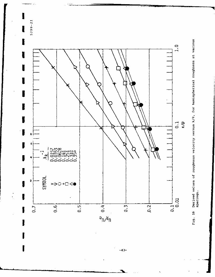
16. Derived values of roughness velocity versus k/6, for1 hemispherical roughness at various spacings. 43

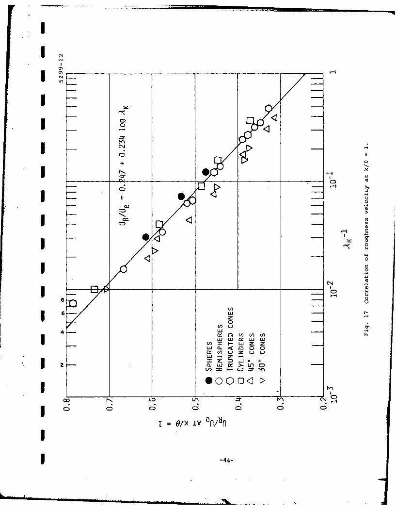
17. Correlation of roughness velocity at k/B = 1. 44

18. Comparisrn of predicted versus actual roughness forpresent result. 461

19. Comparison of predicted versus actual roughness forSimpson's correlation. 47

1 20. Roughness temperature or density scaling law versusvalues from computer model. 50

1 21. Correlation of roughness velocity at k/B = I forcompressible cases. 52

t 22. Computed rough-smooth transition behavior in low

speed flow. 55

1 23. Computed rough-smooth transition behavior versus Machnumber. 56

11v-

I

I

LIST OF FIGURES

Figure Page

1 24. Computed departure from fully-rough behavior for con-

ditions of Holden's experiment (Me =9.4). 58

25. Computed heat transfer augmentation versus skin frictionaugmentation. 60

11111111I

I

-vi-

1

1 1. INTRODUCTION

Surface roughness can play an important role in increasing friction

and heat transfer under turbulent boundary layer conditions. Roughness ef-

fects have been studied extensively over the past fifty years, in connection

1 with applications such as head losses in pipes and other hydraulic equipment,

ship hull drag, airplane drag, and high speed missile drag and heating. This

study emphasizes the effects of roughness character and the behavior of rough-

wall boundary layers under supersonic and hypersonic conditions. Hypersonic

boundary layers tend to be quite thin, which naturally increases the likeli-

hood that roughness will be important. There have been few experimental or

theoretical investigations of rough wall turbulent boundary layers at high

1 Mach numbers. Furthermore, many high speed flight vehicles, such as re-entry

vehicles, are fabricated from composite materials. Since these typically in-

1 volve woven fibers filled with a resin, they present a different roughness

character than would be found on, say, a metallic surface.

1 One cannot adequately discuss the behavior of flows over rough sur-

faces without recalling the classic experiments of Nikuradse,1 in which water

1 was flowed through pipes roughened by sand. In the "fully rough" regime, the

measured friction factor A was found to depend only on the ratio of roughness

1 height k. and pipe radius

1 ) = [1.74 + 2 log10 R/ks]- 2 • (1)

(A list of symbol definitions is given on page 61). This result holds for ks+

1 = UTks/v greater than about 70. Smooth wall behavior prevails for ks+4 5, and

Nikuradse presented a correlation for the intermediate transition regime.

1 Analogous experiments were performed by Dipprey and Sabersky 2 to extend

Nikuradse's results to heat transfer at various Prandtl numbers. Although

1Nikuradse's sand grains were carefully sifted to obtain a relatively uniformsize (diameter = ks), we have no detailed information on the statistics of the

roughened surface that resulted from adhesively bonding the sand grains to the

I smooth surface.

I Some very detailed measurements were obtained by Moffat and co-

workers 3- 5 on the low speed flow of air over a flat plate covered by closely

t ! -1-

packed spheres. Their data include skin friction, heat transfer, and profiles

1 of mean and fluctuating quantities. These results are quite useful for vali-dating theoretical models. However, only one roughness was investigated.

1 Another important class of experiments involves "two-dimensional"

roughness, such as machined grooves or square rods, normal to the flow direc-

1 tion. Betterman6 varied the relative rod spacing by a factor of about three,

and Antonia and Luxton7 made detailed surveys of the turbulence parameters in

1 the boundary layer over this type of roughness. While several authors have

correlated 2-D roughness data along with 3-D or distributed roughness data,

1 2-D roughness will not be considered here. We might expect substantial dif-

ferences in the nature of the flows. With 2-D roughness, the flow is likely

to be dominated by cavities in the grooves between elements, whereas separa-

1 tion should be. less important with distributed roughness. The model presented

below is aimed entirely at distributed roughness, appropriate to the vast

1 majority of practical applications.

1 The available data base on roughness effects in compressible flows is

considerably smaller than that for low speeds. The most extensive set of ex-

periments were those of the Passive Nosetip Technology (PANT) program,8 in

1 which roughened hemispherical models were placed in NSWC Tunnel 8 at a free-

stream Mach number Ma = 5. Heat transfer was measured by calorimeter methods.

1 The roughness, which varied over two orders of magnitude in height, was creat-

ed by grit blasting or by bonding grit particles; a considerable quantity of

1 data were obtained on both roughness augmentation of turbulent heating as well

as roughness-induced transition. It should be emphasized that these tests

1 were performed on blunt nose regions, where the boundary layer edge Mach num-bers are subsonic or modestly supersonic. While there is a substantial varia-

tion of density and temperature across the boundary layer in these conditions,

they certainly are not representative of high Mach number boundary layers.

Holden9 has run tests in the hypersonic shock tunnel at Calspan

(Mo. - 11-13) on 450 cones to which grit was bonded; the boundary layer edge

I Mach number is about 1.8. Higher edge Mach numbers, about 4.8, were obtainedin NSWC Tunnel 2 by Keel,10 on 50cones with sand grains attached by epoxy.

1 -2-

1

In the same facility, Voisinet11 measured the combined effects of roughness

I and mass addition. He created the roughness by covering a porous section of

the tunnel wall with a screen. This provides a questionable simulation of

1 distributed roughness, but is undoubtedly necessitated by the extreme diffi-

culty in fabricating a rough porous surface with controlled permeability.

1 Truly hypersonic tests have been performed by Hill 12 (NSWC Hyperveloc-

ity Tunnel) and Holden 13 (Calspan hypersonic shock tunnel), using grit bonded

1 to the surface of slender cones. Hill's experiments, on a 70 cone at Me =8.1, used three different roughness heights. Holden employed a single rough-

i ness on a 60 cone but introduced varying angles of attack to thin the boundary

layer on the windward side, effectively increasing the roughness effect (Me =

4.4 - 9.4). Despite the general similarity of the conditions for these two

experiments, there are differences in the results that deserve further discus-

sion below.1Investigations on the effects of roughness character, where the shape

and spacing of roughness elements are varied, are rather limited. The classic

experiment was performed by Schlichting,14 on one wall of a water channel.

Various arrangements of roughness elements were used, including spheres,

spherical segments, cones, and short angles, at several relative spacings.

Results were presented in terms of the wall shear and equivalent sand grain

1 roughnesses. Several others have investigated the roughness character effect

over more limited ranges, mostly by changing the spacing for a given shape.

1 Chen and Roberson 15 studied three relative spacings of hemispheres, for air

flow through a pipe. Raupach, Thom and Edwards 16 varied the relative spacing

1 over a factor of four for cylindrical elements (k/D = 1) in a wind tunnel. In

water channel flume experiments, Mirajgaoker and Charlu 17 used stones at six

spacings and Sayre and Albertson18 used baffles (similar to Schlichting's

short angles, but with width = 4 x height), again with six spacings. O'Lough-

lin and Annambhotla 19 used cubes at three spacings, in a wind tunnel. Mul-

l hearn and Finnigan20 examined gravel at one spacing in a wind tunnel. To sim-

ulate plant crop canopy flow, Thom21 and Seginer et al. 22 studied tall, thin

rods (k/D - 100), which provide a major variation in aspect ratio of the

roughness elements.I

I -3-

I

I One series of roughness character tests under supersonic conditions

has recently been conducted by Acurex Corp.2 3 in AEDC Tunnel F. The models

I were 450 cones, with an edge Mach number of 1.7. Seven surfaces were used:

essentially smooth, grit blasted, bonded grit, and four chemically-etched

roughness patterns (two heights, two spacings each). The accuracy of the

measured heating rates may be limited by the fact that Tunnel F was an arc

heated, hot-shot type, with pressure decreasing continuously during the test

time, and by the fact that the roughness characteristics varied over the model

surface.1A great number of methods of varying degrees of empiricism have been

1 developed to predict rough wall drag and heating. The soundest methods start

with Nikuradse's observation that the logarithmic portion of the mean velocity

is shifted downward by roughness. This downward shift, AUI/U., is also di-

rectly related to the roughness-induced inczease in fric tion by the fcllowing

relation (at least for low speed flows)12 )21/2 AU (2

1 )fsjU' (2)1/ s

The velocity shift depends on wall conditions, and thus is a function only of

k+ . The smooth wall friction coefficient generally depends on the Reynolds

number based on some measure of the thickness of the viscous zone (e.g. Ree),

1 as well as on pressure gradient and other geometrical factors (boundary layer

vs. pipe, etc.). In the fully rough regime, however, the dependence of C• Cfsm

on Ree combines with dependence of AUI/U. on k+ to yield a dependence only on

the ratio k/O (or k/R in a pipe), independent of Reynolds number. Note that

I Eq. (2) is transcendental in Cf, since k+ involves Ut = VTw-l p. Also, the

above equation cannot be applied directly to compressible flows.

1 For sand grain roughness, the velocity shift in the fully rough regime

is

II

I

I -4-

NU11-=5.6 log ks+ - 3 . (3)

1UDvorak 2 4 ,25 first extended this relation to describe variations in roughness

1 character

AU1

1 - 5.6 log k+ + f(X) , (4)UT

1 so that the equivalent sand grain roughness (k.) is related to the actual

roughness height (k) by

1 5.6 log ks/k = f(X) + 3 * (5)

Here. f(X) is some measure of the roughness density. Dvorak correlated the

available data with X-1 being the fraction of the surface covered by roughness

(the base area of roughness elements per unit underlying smooth surface area).

Simpson26 obtained improved results in terms of Xk, the inverse of the pro-

jected frontal area of the elements per unit surface area, and others2 7 ,28

1 have used similar variations of the Dvorak approach.

1 Figure I shows Simpson's roughness dens4ty correlations. The two

straight line segments are the same as Dvorak's (in terms of X rather than

Y). Note that the roughness effect has a maximum at Xk = 4.70, which corres-

ponds to spherical elements with an average separation of 1.9 diameters. Note

also that nearly all of the data to the left of this maximum, for more closely

1 packed elements, are for two-dimensional roughness. Simpson notes that the

flow in this regime may be dominated by cavity flow between the elements, and

1 speculates that this decrease in roughness effect with decreasing spacing may

not occur for 3-D roughness. We shall return to this matter in some depth be-

1 low.

For compressible flows, Dvorak2 5 applied the same compressibility fac-

I tor used for smooth walls (these are surveyed in Ref. 29). Equation (2) is

I-II -5-

1 lC1 C-)

< -0LLJ z m (n z ,

C 00

I- :j,01(/44

(i~~-0

-

U 0

2 - 0

46-4

1

!used to compute an incompressible friction coefficient, with Cfsm based on

1 Fe.Ree and AUj/U T based on the actual wall conditions; the compressible fric-

tion coefficient is then obtained by dividing the incompressible value by FC.

However, this procedure is not necessarily logically consistent with the in-

compressible behavior. If AUi/UT really depends on local wall conditions,

then Eq. (2) would apply directly to compressible situations, simply by in-

serting the appropriate compressible value of Cfsm* But Dvorak found this al-

ternative to yield poor agreement with data.!A number of investigators have developed more empirical methods for

1 reentry applications. One of these, which is well-known and has been derived

from both low speed and high speed measurements, is the version developed by

1 Acurex Corp. and contained in the ABRES Shape Change Code. 30 The roughness

augmentation of skin fricticn is described by an influence coefficient, by

which the smooth wall value should be multiplied, independent of compressibil-I ity:

If = 1 + 0.5 fl(k/e)g1 (x) (6)

1 fl(k/e) = 1 + 0.09 k/e + 0.53(1-e-k/e)

g1X) -v + 1.5(1-e-X) for X > 0

1 =0 for X 4 0

X = log(k+/15.5) (Based on smooth wall Cf).1While this relation provides a smooth transition between smooth and rough wall

1 behavior, it does not obviously reduce to the dependence observed by Nikuradse

An the fully rough regime, in that the drag is predicted to depend on both k+

and k/8. Dahm31 has recently developed a new correlation for roughness ef-

fects, involving a "two-layer" model.

1 Another issue of considerable uncertainty is the relation between heat

transfer and skin friction. For smooth walls, the mechanisms of turbulent

1 heat and momentum transfer are quite similar and the heat transfer and skin

friction coefficients are closely related. But with rough walls, form drag

11-7-

on the elements has no analogous thermal mechanism. This provides an intui-

1 tive explanation f or the common observation that roughness causes smaller in-creases in heating than in friction. Owen and Thompson32 developed a correla-

1 tion for roughness-dominated heat transfer, following lines suggested by as-suming cavity flow between the elements. However, the result involves prima-

rily k+ and it is not clear whether this behavior is consistent with the well

1 known dependence of skin friction on k/6 rather than k+. The heat transfer

correlation used in the ABRES Shape Change Code30 is simple and pragmatic - the

1 numerical factor 0.5 in Eq. (6) is replaced by 0.3.

I The analyses to be presented below are based on a fairly basic model

for rough wall boundary layers, wherein a Reynolds stress turbulence model is

combined with a form drag 'description for the effect of roughness elements on

thto flow. The computer itodel is used ir- two ways; 1) it is compared againstrelevant data to establish the validity and accuracy of the theory and to of-

1 fer explanations for observed trends; and 2) it is used to develop correla-

tions for engineering applications by suggesting scaling laws and by providing

1 numerical data to be correlated. In previous papers,3 3'34 we showed compari-

sons with a good portion of the available measurements and presented some pre-

1 liminary scaling laws. Here we will analyze some of the most important dataon roughness character and compressibility, and shall present correlations

1 that should have widespread utility.

1

I2. ROUGH WALL BOUNDARY LAYER MODEL

The basic model for rough wall turbulent boundary layers is the same

I as that used previously, 33 ,34 and we shall only outline the most relevant fea-

tures here. The turbulence model is a Reynolds stress or second-order closure

1 method, which computes both mean and fluctuating velocities and temperatures.

The dependent velocity variables are the mean velocity vector Ui, the Reynolds

S-tress tensor uiuj', and the isotropic dissipation rate 0. The analogous

thermal variables (temperature or, more precisely, enthalpy h) are the mean

I enthalpy h, the mean square fluctuating enthalpy h '2, and the Reynolds heat

flux vector ui'h'. Under the boundary layer approximation, this set of vari-

I ables reduces to U, V, u ' , v ' , w' 2 , u1, 0, h, h- 2, u-h', and vh'. The

closure approximations that are used to derive the required equations are

somewhat standard at this time. The formulation has been successfully applied

to a variety of smooth wall boundary layer and free sheaz flows. Predicted

smooth wall skin friction coefficients are generally within 10-15% of accepted

values, except for a few cases with very large density differences, to be

noted below.1Our model makes the basic assumption that the force on roughness ele-

1 ments can be viewed as form drag. This implicitly requires that the flow ap-

proaching an individual element be attached. As already noted, cavity flow is

likely to prevail with 2-D roughness; for this reason the present model should

be more appropriate for distributed roughness.

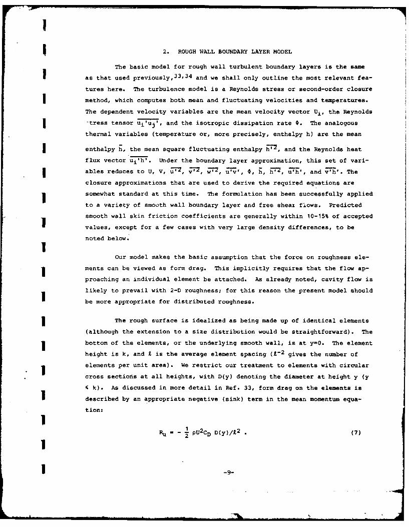
1 The rough surface is idealized as being made up of identical elements

(although the extension to a size distribution would be straightforward). The

1 bottom of the elements, or the underlying smooth wall, is at y=0. The element

height is k, and £ is the average element spacing (L-2 gives the number of

elements per unit area). We restrict our treatment to elements with circular

cross sections at all heights, with D(y) denoting the diameter at height y (y

4 k). As discussed in more detail in Ref. 33, form drag on the elements is

1 described by an appropriate negative (sink) term in the mean momentum equa-

tion:

11Ru pU2 (~

R pU2 CD D(y)/X2 (7)

1 -9-

I

A drag coefficient value of CD 0.6 is roughly appropriate for elements such

1 as cones or hemispheres. In addition, there should be source terms for turbu-

lent kinetic energy and dissipation, describing the tendency of roughness to

1 increase velocity fluctuations. These terms, which are discussed in Ref. 33,

are not very important compared to the indirect effect of roughness to in-

crease the turbulent energy by increasing the mean shear.

Except in the Stokes flow regime, heat transfer to an element should

1 be small. Therefore, the only roughness term appearing in the thermal equa-

tions is a source term for the mean static enthalpy. This term is constructed

1 so that, in combination with Eq. (7), form drag does not alter total enthal-

py.

1Rh = + 1/2pU 3CDD(y)/. 2

. (8)

1It is also necessary to account for the blockage effect of the rough-

ness elements. At a given height, the fraction of the flow area normal to the

x direction is 1-D(y)/I. Terms that act in the streamwise direction, such as

the convective operator pua/ax, are multiplied by this factor. Terms that act

1on planes normal to the y direction, or that act on a unit volume, should be

maodified by I--D2/4X2. However, tae ioughness term disnusred above arr al-

1 ready based on the total volume, rather than the available flow volume, and

need no such factor. If the entire equation is divided by B(y) = 1-wD2/412, a

1 relatively simple result is obtained. For example, the mean momentum equation

becomes

f(y)pu 2-u + pV u - f(y) B + - auax ay ax Bay ay

a . u . lpU2CD B1(9)ay -10

I -i0-

1

Iwheref(y) = 1-DI/4 (10)

1-irDZ/41Z

1 The function f(y) contains the main effect of blockage and may be ab-

sorbed in the definition of the stream function that is introduced to elimi-

1 nate the normal velocity

If(y)PU PVay ' , - pV . (11)

I Note that if the elements are packed so tightly that they are touching over

some range of y, then D = I and f(y) = 0 over that range. Our formulation

1 forces the velocity to remain zero up to the height where D < £ and the flow

is unblocked. Of course, common sense would dictate redefining y = 0 as the

lowest point where the flow is unblocked.

A major advantage of this model is that solutions are obtained for

both velocity and thermal variables. Heat transfer is obtained directly,

without invoking a Reynolds analogy. Finite difference solutions are obtained

S1 using the obvious boundary conditions. Fluctuating quantities are zero at the

base of the wall, y = 0. At the outer edge, fluctuating quantities are zero

for a boundary layer or obey a symmetry condition for a channel flow. For

numerical solutions, the equations are first transformed to the stream func-

tion coordinate, guaranteeing mass conservation and eliminating the normal

1 velocity, V.

1 The transverse coordinate is normalized by the edge value of the

stream function so that additional mesh points need not be carried in the free

stream to allow for boundary layer growth. For proper resolution of the

region near the wall, a linear mesh in the logarithm of the stream function is

used. The finite-difference equations are solved with a block tridiagonal

1 Newton-Raphson technique.

1

1

1

1 -11-

It should be noted that the use of such a model is not unique to this

study. Lin and Bywater35 have used the present form drag treatment in a two-

equation TKE model, and generally obtained results superior to those obtained

I from lower level approaches. A very similar model has been developed by Wil-

son and Shaw3 6 to analyze transport processes in plant canopies. A crop of

I corn plants, or a stand of trees, represents an attractive geometry for the

form drag model. For such applications, it may be necessary to account for

the effect of plant motion on the turbulent energy budget.

112

I3. SPECIFICATION OF ROUGHNESS CHARACTERISTICS

An important aspect of predicting or analyzing roughness effects is

the proper specification of the roughness characteristics. For laboratory ex-

periments in which identical elements of a simple shape (spheres, cones, etc.)

are attached to a smooth surface in a regular pattern, the required element

height, shape and average spacing are obvious. Such is not necessarily the

case for grains of sand or grit, sifted to a narrow size range and applied to

the surface with an adhesive. The details of the bonding technique and the

departure from sphericity of the particles can affect the roughness param-

eters. Real surface materials introduce even greater uncertainties. Here we

present the method for deriving the roughness specifications, required for our

model, from profilometer surface measurements.

1 A profilometer measurement of the surface in question is required.

This consists of an irregular trace of height y, above some reference, as a

function of distance along the line over which the stylus was traced. It will

1 be assumed here that all elements are identical in size and shape - one could

derive a more sophisticated analysis for situations where a significant varia-

I tion in element sizes is expected. It is also assumed that location of rough-

ness elements has at least a moderate degree of randomness.

Figure 2 sketches a typical profilometer curve. From this curve, it

is necessary to form a probability of exceedance distribution, P.E.(y), which

is simply the fraction of the trace with heights greater than y. one must al-

so identify peaks and compute the average spacing between peaks, LP. Finally,

one must define the height y = 0, corresponding to the effective floor of the

roughness.

1Now, any element located within a roughness element base radius on

either side of the profilometer line should be detected and counted as a peak.USince L-2 is the number of elements per unit area, a profilometer trace of

length Lt should detect D(O)Lt/X 2 peaks. The number detected is Lt/L, by

1 definition of the average peak spacing. Equating these two quantities gives

1 2 =D(O)Lp (12)

11-13-

(N

re

04

4CEn

sm..dm. Il

Since the roughness statistics are taken to be uniform, the probabil-

ity of exceedance of height y along a profilometer trace must equal the frac-

tion of the surface area above that height. The latter fraction is simply the

cross-sectional area of an element at the height, r/4 D2 (y), multiplied by the

density of elements, X-2 .

P.E.(y) = D2 (y)/L 2 (13)

Equations (12) and (13) are sufficient to reconstruct the roughness

characteristics. From the P. E. value at y = 0 (which should be less than

w/4 to allow D(O) < £), Eqs. (12) and (13) yield D(O) and £. Equation (13)

can then be used to obtain D(y) for greater heights.

Some examples of the roughness specifications that result from this

process will be given below, for grit-bonded surfaces. In practice, some

judgement is required to identify the "floor" of the surface (y = 0) as well

as to identify peaks in the profilometer curves. With sufficient statistics

(e.g., the profilometer traces should intersect on the order of 100 or more

elements), the practical effects of such uncertainties is small, because the

portions of the elements near the base do not contribute greatly to the total

drag.

-15-

I

4. COMPARISONS WITH ROUGHNESS CHARACTER DATA

As indicated in the Introduction, the most extensive experiment on

roughness character is the Schlichting14 study of various roughness patterns

on one wall of a water channel. In Ref. 34 we made some preliminary analyses

of Schlichting's data, using boundary layer solutions at the proper value of

Re6. Here in Figs. 3-6, we show more appropriate solutions for the proper

channel geometry.

For spheres, Fig. 3, the rough wall boundary layer model agrees ac-

ceptably with the measured friction coefficients, the worst error being about

25% at Xk = 3 or X/D - 1.5. At the closest packing, we specified hemispheres,

since the bottom half of spheres would be completely blocked. This is done

for numerical convenience, to avoid singularities associated with f(y) = 0 in

Eq. 9. According to our calculations, blockage of the bottom half-sphere is

responsible for most of observed reduction in drag as L/D + 1. For compari-

son, the Dvorak/Simpson correlations (which are identical for spheres) are

also plotted.

For spherical segments, which are somewhat less than hemispheres, pro-

bably to simulate rivets, the computer code gives excellent results (Fig. 4).

Note that the code shows only a very modest maximum in Cf, in contrast to the

Dvorak and Simpson correlations. Good agreement was also obtained with Chen

and Roberson's 15 data on hemispheres, although they investigated only very

large roughness spacings.

For Schlichting's cones, shown in Fig. 5, our model is slightly low.

Closely packed cones were not tested, but again the present model shows no

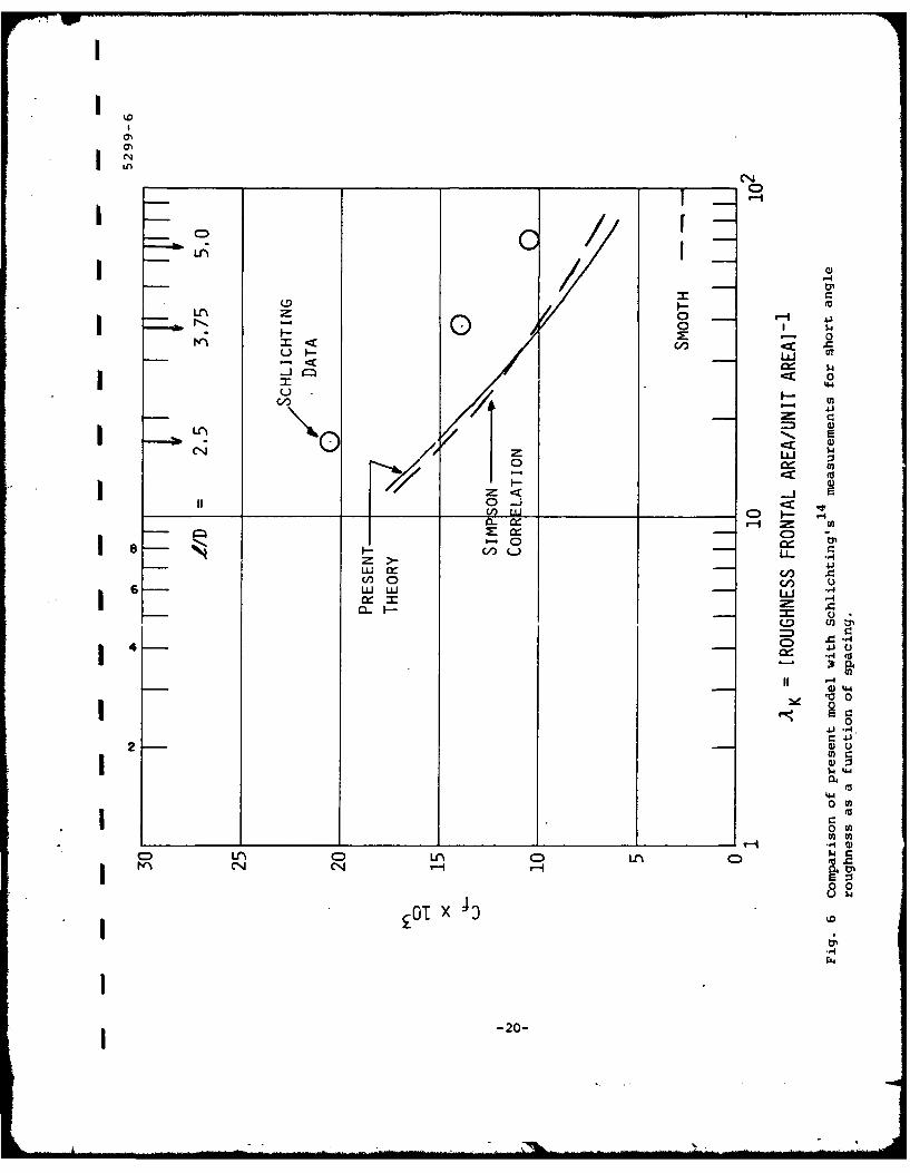
pronounced peak. The short angles of Fig. 6 were simulated as cylinders of

the same height and width in our calculations. The model is noticeably low

here, for unknown reasons. However, we would expect less accuracy for cases

with non-circular roughness, and similar errors would be expected for the baf-

fles of Sayre and Albertson."8 Generally good agreement was achieved with the

data of Raupach, Thom and Edwards, 16 on cylinders (height ± diameter), as

shown in Fig. 7.

Figure 8 compares our results with the observations of Mirajgaoker and

Charlu.17 We used the channel flow version of our model to simulate their

I -16-

000

zn w

0 0

--0

-41

~4

LUL a).~ e

0~ /U- U

8 a_-2:

0 w0C

t;

- 0 0

~OT X 4

-17-

Ln

C14

C/ -4

I--

/0.

-L 0

CN/ j

C:)

cn

8) 00j

41

44

I0 le 4

00

CL 0t7

LA u <A c A 0

I~ £0$44-18-

CN

Ln

I - 4LA 0

0

I-L

LLi

6 Lo

Ul

LLJ

0 02

41~C)4

op CD -4

0(

II

LA 00 -40LA0

CN c 0

w 4) uLOT Mr

-19- :

I",

CD

-4

(0 =U OT.0 v-I

4.4

41N C:

C4 z 0$00CNJ z

x C)

p.--

u L;

0

0

44 .-4.

2 (

%&4

.

U0

-200

C14 0

01) 0

0'I cr C

(n 0LLJ LLI 0

04

I-4

(1)0 0_act

UL U

0) u

+-

I-0) 018 LL 4

4J

40)

0 0)2

0

w) .14.. 4 I$4I54'

OUTX

-21-

Iw-

0

4

IL (0

+

LLI C-

ID 9

0 L 0

X:' 0 J

< 2U

18 rr = - C- r.

0 cc - % L

4J to

04

4-44 040 t

*2 01>z

F- C-1)0

0~~~ 0 )0

OT1 X

-22-

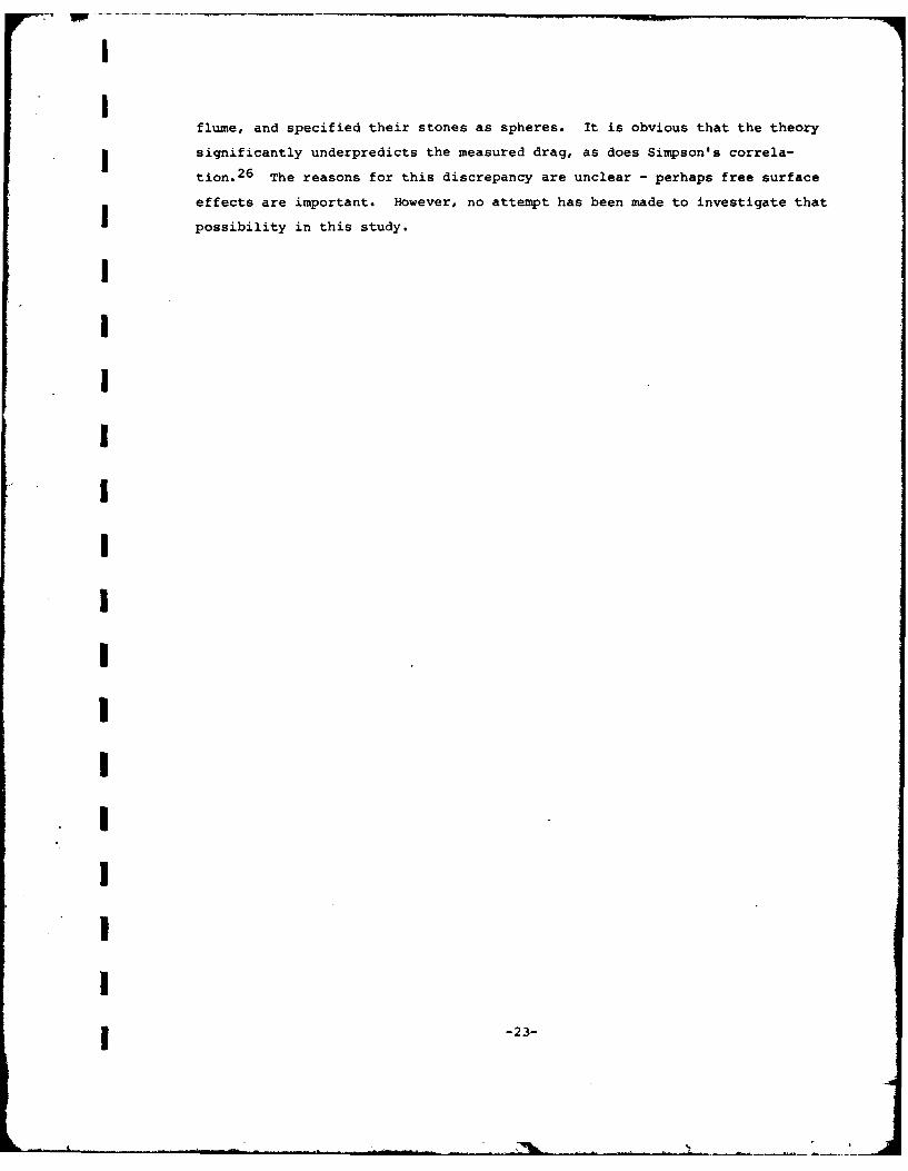
I

Iflume, and specified their stones as spheres. It is obvious that the theory

g significantly underpredicts the measured drag, as does Simpson's correla-

tion.2 6 The reasons for this discrepancy are unclear - perhaps free surface

effects are important. However, no attempt has been made to investigate that

I possibility in this study.

I

I

I

I

r° I

I

I

III

I1

I

i -23-

nI 5. COMPARISONS WITH COMPRESSIBLE ROUGHNESS DATA

The effect of surface roughness in compressible flow conditions re-

mains poorly understood, perhaps largely because the available data base is

rather fragmentary. In Ref. 33 we showed extensive comparisons with the PANT

I data on hemispherical nosetips at supersonic velocities, and we also demon-

strated 34 satisfactory agreement with Keel's data 10 at Me = 4.8. Here we

shall present analyses of the recent measurements of Holden and Hill. Some

preliminary comparisons were given in Ref. 34, but the diagnostic techniques

and roughness characterizations have recently been extended and refined, per-

mitting more definitive analyses at this time.

I One interesting series of tests by Holden9 were performed on 450

cones, at an edge Mach number of 1.8. These tests illustrate the importance

of the method of applying grit to the model surface. Holden's most recent

studies used a two-sided tape to apply the particles, whereas earlier methods

used Krylon spray adhesive. Holden 9 kindly supplied us with profilometer

traces of the surfaces prepared in each way from identical "4 mil" grit.

Figure 9 shows the average elements derived by the method presented in Section

m 3. There is clearly a significant difference, with the two-sided tape yield-

ing greater roughness height and density. Subsequent discussions with Holden

m led to the conclusion that various effects such as agglomeration can affect

the bonding pro-ess. It is not sufficient to use the nominal grit or sand

grain size as a measure of the roughness size.

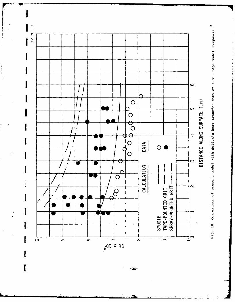
In Fig. 10 we compare the present model with Holden's measured heat

transfer data for the 4-mil tape mounted roughness. A significant error is

seen in the absolute level of the smooth and rough wall computations. This

1 error seems to be appreciable for cases with low values of Tw/Te, at modest

edge Mach numbers. At hypersonic speeds, viscous dissipation maintains high

1 teperatures.throughout most of the boundary layer and no such overprediction

is found. This error, then, occurs for cases with extreme density or tempera-

1 ture variations across the boundary layer. Despite careful examination, we

have not been able to remedy this discrepancy. Numerical accuracy does not

seem to be the issue, and we can only speculate that existing turbulence clo-

sure approximations are inadequate in situations with large density gradi-I ents.

1 -24-

-4

I:3 ~ 00 F-- - 0

0

U)

tr.

0

-r-

0

E

0

$~4

I _ _ _ _

t;.

-25-

I0

_____ ___________ __________ O

U4

C:))

Q)

04

Url 0

C> LJ cc

Ii. 0- w ~ ,

C) H

___~O X_ IS -

L260

I

IIf one were to scale down the magnitude of the calculations, the ex-

tent of the predicted roughness augmentation would agree rather well with

Holden's data for spray-mounted roughness. As also indicated, the model pre-

dicts less increase in heating for the Krylon-mounted roughness.

Two very significant experiments under similar hypersonic conditions

were performed by Holden 13 and Hill, 12 on slender cones at Me = 8-10. Holden

used a single 10 mil (nominal) grit, and obtained measurements on the wind-

ward ray at angles of attack from 0o to 160. To confirm earlier results with

thin film gages, he used calorimeter heat transfer gages, in addition to skin

friction gages. Hill used three different roughnesses, from nominal grit

sizes of 11, 37 and 65 mils. Both experimenters provided us with profilometer

traces, from which we derived the roughness parameters.

Figure 11 shows the roughness element specifications derived from the

profilometer traces. Hill's method of application appears to result in ele-

ments that are more vertically aligned and more closely spaced on a relative

basis. For three of these surfaces, the derived roughness height is close to

the average grit diameter, but is very much less for Hill's "65 mil" grit.

This finding emphasizes the need to perform careful characterizations of actu-

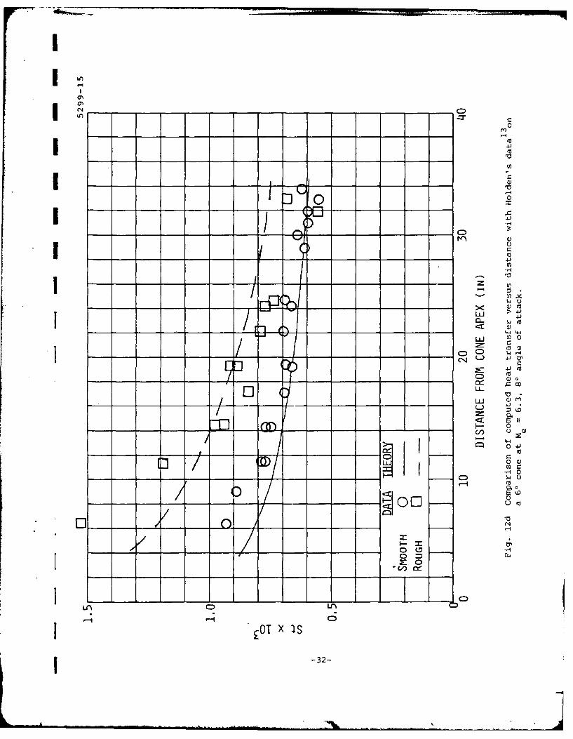
al rough surfaces.!Figure 12 compares the present model with Holden's measurements. For

the cases at angle of attack, we used an equivalent cone approximation to de-

scribe angle of attack effects, which might be less accurate at higher angles.

Several trends are evident in Fig. 12. Roughness causes a greater increase in

skin friction than in heat transfer. At a = 00, Holden's results show little

roughness effect at the larger downstream distances, whereas a modest effect

Iis predicted. Greater increases, and better agreement between theory and

data, are seen with increasing angle of attack.IThe corresponding comparisons with Hill's heat transfer data are shown

in Fig. 13. The predicted roughness heating is similar for all three of

Hill's roughness. The 11 mil case is somewhat over-predicted, while the other

two cases are underpredicted at greater downstream distances. Both theory and

data indicate slightly higher heating values at 37 mils than at 65 mils. This

behavior is compatible with the derived roughness characteristics shown in

Ii -27-

II

N.N$4

0)

0)

C:)C C

L1C-4

- -~ 1 --28-

0

- - - 0

'0

IV

Liii

.14cmi 1-

________

____ ___ ___ 0.. LI)m

00 0

S0V/) LL

-j --.J-1

00--- - _ - _ - _ -- 4J-4

0

00

to)

04-

0-4)

-r( D00 Lo_0 C

-29-

HC'(N

41

In-

COs

bo -'T X

0LLU Q) 0

44

L-))

CN0 CN/0 Z .)

LL a

)D LU Q

4-1

000 0

U o

-: 00 LO _-x CN

O T x I -30-

IDI

~~0

'U4J

Zo L

g 0 -Lr n4

C I

0 0 u

0.

U ODIn

(N

-3.1-

IX

0 MM0

-1-II-- -- - 1 C:)

0

_ IIt

CC)

z 4 u

Li.J u40

LU) C) )$

04

- - I- 0

w-44

0 4

(n s

- - 00 0

0 C~

LOT I S

-32-

0u

00

14

00

-41

-a

U-'

Ll

LU ~.0.

CD U4

LL 0

() 0

44 3~~7L~~ V - z.-

-% 0

04~ r-4-C

4

-33-

1 41

-toCL

o

1 4)C/ o

mlC 0 0 4C=) 0

CN 0

o Q 44).-

X0

OT IS

-34-)

00

o< 0

LL-4

__ 'dO 1-4

U- 0-~ a)~

S U)

Oi 1 4)

to

4-4

CD'

I -4tO__IS

443

-35-

I!

Fig. 11, which showed the same height but greater spacing for the 65 mil grit.

One puzzling aspect of Hill's data is the tendency of the rough wall heating

rates to be essentially independent of distance. If anything, we would expect

the rough wall measurements to decay at a greater rate than the smooth wall

data, since k/6 decreases with increasing distance.

The 10 mil data of Holden at 00 angle of attack and the 11 mil data of

Hill are significant, in that very little effect of roughness is evident in

either case. The present theory and most existing correlations predict at

least a moderate effect. It is suggested below that relatively modest rough-

ness Reynolds numbers are responsible for this behavior. The quantity k+ is

50-70 for either case, but is much larger for Holden's cases at nonzero angles

of attack and for Hill's cases at larger roughness. Such k+ values are only

slightly below the fully-rcugh requirement of k+ = 70 for incompressible

flows, However, careful examination of our computer results indicates that the

transition values should increase with increasing Mach number, to be discussed

more extensively below.

-36-

6. ROUGHNESS SCALING LAW

While the model presented above yields good general agreement with the

available data, it is not particularly useful for engineering purposes. The

computational cost of running the computer code is modest. However, it is im-

practical to expect other users to become familiar with the program, which in-

volves finite difference solution of many simultaneous, stiff partial differ-

ential equations. What is needed is an algebraic recipe that can be readily

understood and applied to practical problems. our computer model can be use-

ful in developing such an engineering method in two ways: 1) numerical solu-

tions can be examined to determine the dominant physical processes and 2) the

code can be exercised to generate a base of numerical data covering the range

of input parameters far more thoroughly than do the available experiments.

The key to developing scaling laws for roughness effects lies in the

computed mean velocity profiles. For the vast majority of cases considered,

the mean velocity is quite uniform over much of the range y < k. An example

is shown in Fig. 14, from our solution for Schlichting's closely pac1red spher-

ical segments. Near the top of the elements the velocity profile increases

and blends into the log region, and the velocity must decrease towards zero as

y +* 0. But the velocity is remarkably constant for most of the region y < k.

The exceptional cases, in which a range of uniform velocity is not evident,

generally involvi such short or sparse rouc,-hnesses that the smooth wall pro-

file is hardly altered.

It must be admitted that this velocity behavior was not anticipated in

our model development. Physically, for y < k the turbulence is simply diffus-

ing toward the base of the wall and dissipating. Perhaps an approximate model

could be developed, for example by a three-layer approach (the constant veloc-

ity region, the log region, and the outer region). There is little experi-

mental evidence to confirm or deny the predicted behavior, since it is gen-

erally not feasible to measure flow properties between roughness elements.

Chen and Roberson15 show a profile that increases by only 10-20% in the range

0.2 < y/k < 1, for hemispheres at an average spacing of 4.5 diameters. This

velocity profile behavior is apparently well known in the study of turbulence

-37-

CN 4

3 04

-4

0

04

tw

0

-~ -4

0

0

1-n-4

-38-

I7II

in plant canopies, and Raupach and Thom3 7 quote two measured wind profiles in

plant canopies (a pine forest and a maize field) that are quite similar to

that of Fig. 14.

The wall shear is given by

k 2Cf =Cfsm + f pU2 C D f(y) D() dy , (14)

0 PeUe L2

(the blockage factor f(y), defined in Eq. (10) , enters through the stream

function). Now let us approximate U as a constant U = UR. For compressible

cases, p will be related to U, and hence is also constant p = PR. The block-

age factor generally varies slowly with height and will be approximated by its

value at k/2. Since the integral of D(y) is simply the frontal area of the

roughness element, Eq. (14) reduces to

Cf =Cf + P 7 ' (15)ee

which is the basis for deriving the appropriate scaling laws.

6.1 Incompressible Fully-Rough Flow

Equation (15) may be contrasted to Eq. (2)

(2 )1/2 = /2 - _U,- 9

(2)

-39-

I For sand grain roughness, the velocity shift in the fully rough regime is

5- = 5.6 log k,+ - 3 .(3)

1*

The smooth wall skin friction involves the Reynolds number based on some meas-

ure of the width of turbulent layer. We shall select the momentum thickness e* as the appropriate thickness. * To a very good approximation

( 2) 12= 5.6 log Ree + C,(6

* where C depends on flow geometry and pressure gradient. Putting Eqs. (3) and

(16) into Eq. (2) shows that the skin friction is solely a function of k/e for* fully rough conditions

* (2)1/2 -5.6 log (2)/

-3+ C -5.6 log k5 / (17)

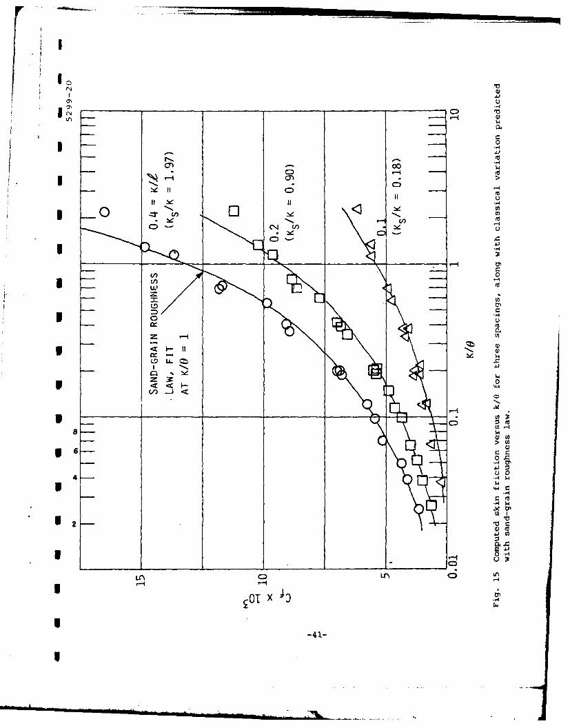
We have run our computer code over a wide range of parameters such ac

roughness shape and spacing. We first confirmed that Cf is a function only of

k/e, within the available numerical accuracy. Figure 15 shows an example of

the computed behavior, for hemispherical roughness elements at three relative

U spacings; k"" varies substantially. The spread of the computed points for each

spacing is indicative of the numerical accuracy. The curves represent Eq.

5 (17), with k. chosen to match the computed values at k/e = 1.

U 'The boundary layer thickness is most analogous to the radius of a pipe or

half-height of a channel. However, boundary layer models compute 6 inaccu-rately (in our case) or not at all (in most integral methods). The displace-

3 ment thickness 6* is also not a good measure for compressible situations, forwhich it becomes quite sensitive to the density ratio e-rss the boundarylayer.

1 -40-

Mom

C)-

30)C)

CD'-* 41-4

I00'

4-)

< Q0

40'

0 0

,4 $.4

I ~4

C L- -

LOT X 4

I

Equations (15) and (17) represent two alternate views of roughness ef-

fects. Equation (17) explicitly shows the dependence on ks/0, but contains no

information on roughness character; Eq. (15) is useful for displaying rough-

ness character. If Cf is to depend only on k/6 and roughness character, then

UR must depend on the same quantities and must also depend weakly on Re8 in

such a fashion as to cancel the weak dependence of Cfsm on Rea. In practice,

we have correlated UR from computed values of Cf at any Ree and k+ in the

I fully rough regime, specifying Cfsm as the flat plate value at Re8 = 105. So

long as the same value of Cfsm is retained, the resulting correlations for UR

3 can be used at any Re8 or k+ in the fully rough regime.

i we have developed a numerical data base for roughness character ef-

fects from boundary layer runs with a variety of roughness shapes and spac-

ings. The shapes considered were hemispheres, spheres, cylinders (diameter

I = height), 300 (half-angle) cones, 450 cones, and truncated 300 cones (top

diam = base diam/2). Spacing was generally varied from k/k = 0.1 to as close-

ly packed as numerically feasible. From the computed values of Cf, along with

CD = 0.6, PR/Pe = 1, Cfsm = 1.81 x 10- 3 for our flat plate solution at Re8

5 = 105 , and the appropriate values of f(k/2) and Xk, we then solved Eq. (15)

for UR/Ue . An example of the derived values is shown in Fig. 16 for hemi-

3 spheres. The straight lines are drawn as an aid to the eye; UR/Ue cannot be

precisely linear in log k/6 and still have consistency betwsen Eqs. (15) End

(17.)

The other shapes investigated yield plots quite similar to that of

5 Fig. 16. In fact, if one were to approximate the numerically derived values

of UR with straight lines as indicated in Fig. 16, the height and slope of the

lines are almost solely a function of Xk and quite insensitive to elementIIshape. Such a correlation for UR as a function of k/6 and Xk could then be

I used in Eq. (15) as a useful engineering tool. However, it is more precise

and more compatible with existing methods to correlate UR vs. Xk at a fixed

value of k/6 (such as unity) and then use Eqs. (15) and (17) to derive the ef-

fective sand grain roughness. In Fig. 17 we show the derived values of UR at

k/6 = 1 for all of the shapes considered. A modest shape dependence may be

II -42-

C'44

L)

0

"-4

6 J-4

Iuf _ _4_ __L __ _ _ __r-- U,->u8Hz C5C -Nr,

4--

C: C)C )CUDC

I 02 tN00 -

Z-;-:~ MX>O +0 LC vI

0000D CDC) DC

-43-4

CNq

1 01

r-r_o0

040

6 - w

041 0

(nN4- -4

m 0 muIU - 4

2 CI w 0:> N)C

I W-44-

I

Idetected, with conical elements tending to fall below the more blunt shapes.

I The correlation suggested in the figure best fits the more blunt shapes, which

may be more representative of actual surface roughnesses; also, our theory

i tends to underpredict the roughness effect observed for cones by Schlicht-

ing. 14

9 If one inserts the indicated correlation

UR- = 0.247 + 0.234 log Ak (18)e

along with Cfsm = 1.81 x 10- 3 , C = 5.24, and CD = 0.6 into the above equa-

tions, the following equations result for the ratio of sand grain to actual

5 roughness height,

Cf[ = 1.81 x 10 - 3 + 0.6(0.247 + 0.234 log Xk)2 f(h) _L (19a)

I 5.6 log ks/k = 8.50 - + 5.6 log (19b)fi) \ fi/

p Figure 18 compares the value of ks/k predicted by Eq. (19) with the

actual observed values, for a number of experiments involving roughness char-

i acter. Two sets of data are seriously underpredicted by the present correla-

tion (as well as by the computer model - cf. Figs. 6 and 8): Schlichting's

short angles 14 (baffles) and the stones of Mirajgoaker and Charlu. 17 We have

I no explanation for these discrepancies. The tall rods of Seginer et al. 2 2 and

Thom21 are rather substantially underpredicted.IFor comparison, Fig. 19 shows a similar comparison for the correlation

i of Simpson,26 a refinement of Dvorak's correlation. 24 The general degree of

correlation is comparable to that of the present result. The short angles of

Schlichting and stones of Mirajgoaher and Charlu are again underpredicted; the

rods of Seginer are handled decently, but those of Thom could not even be

plotted on the figure. It is most important to note that the Simpson (and

I Dvorak) correlation is not accurate for closely packed roughness elements.

I

I -45-

. . . .-L. . _ . . . . . .. . . . . . . . . . . , . .

10 5299-23

I ±20% I NI Cf (APPROX)

*L 00

L 1 0

U)j 1 0

0.1 LEGEND8 00 SCHLICHTING - VARIOUS

6 - 0 RAUPACH - CYLINDERS0 0'LAUGHLIN - CUBES

4 CHEN - HEMISPHERES

0 -- SAYRE - BAFFLES5 0 MIRAJGAOKER - STONES

2 -7 MULHEARN - GRAVEL

5 0SEGINER - RODS

>THOM - RODS

0.01 011 24 6 -8I10

5(KS/1K) Observed

5 Fig. 18 Com~parison of predicted versus actual roughness for present

reut

-46-

1 5299-2410

+ I l 20% IN

E Cf (APPROX)

I0

1 0 0

4 -J

SCLCTN 0 AIU

0.1 0 CHLN G - VARIOSES

-J SAYRE - BAFFLESZIsMARAJGAOKER - STONES

2 17MULHEARN - GRAVEL

(j JSEG INER - RODS

01 D THOI - RODS

S 0.1 1 i 10

I(K s/K) Observed

Fig. 19 Comparison of predicted versus actual roughness forI Simpson 's correlation.

-47-

I

The points for Schlichting's closely packed spheres, spheres with L/D - 1.5,

and closely packed spherical segments all fall outside the indicated ± 20%

error band in Fig. 19. Most of the available experimental data on roughness

character have been obtained with relatively sparse roughness patterns. The

Simpson/Dvorak correlations are fine tuned to the data base, but do not have

the benefit of sufficient distributed roughness data at greater roughness den-

sities. Use of the straight line segment with positive slope in Fig. 1 leads

to the poor results cited and Simpson questioned the validity of that portion

of the correlation for 3-D roughness. Hence, for relatively closely-packed

roughness (say X/k 4 1.5), which corresponds to most surfaces of practical in-

terest, the correlation derived here should be the more reliable.

6.2 Compressible Flows-Fully Rough

Compressibility effects generally reduce friction on both smooth and

rough walls. Smooth wall friction coefficients are generally computed from

"transformation functions," Fe and Fc . As reviewed in Ref. 29, an equivalent

incompressible coefficient is computed at the effective Reynolds number Fe*

Re8 , and is then divided by Fc to obtain the compressible coefficient:

Cfsm = Cf (Fe * Re8 ) (20)

As noted above, Dvorak 24' 2 5 used Eq. (2) to obtain a rough wall incom-

pressible friction coefficient, evaluating Cf sm at Fe * Ree and AUj/U T at the

actual value of k+; he then divides by Fc according to Eq. (20). Note that Fe

plays a very small role - Fe is usually near unity and Cfsm is insensitive to

Reynolds number. If Fe plays no role, then this procedure guarantees that the

percentage increase of friction is independent of compressibility, at fixed

k/O. Our model, however, predicts a rather different result - that the rela-

tive effect of roughness decreases with increasing Mach number.

In the present model, one obvious effect of compressibility is through

the density. At high Mach numbers, viscous dissipation causes high tempera-

tures within the boundary layer. Because roughness reduces velocities within

II

~-48-

I

the boundary layer, even higher temperatures can be expected. To estimate the

roughness density, we evaluated the relation between total enthalpy and veloc-

ity in the output from a large number of computer runs at edge Mach numbers

between 0 and 10. A linear relationship was found to be quite accurate

H-hw U (21)h Ue- w e

as it is with nearly any turbulent situation. Then, with perfect gas rela-

tions it follows easily that

T -1

Y-1 M2 R (22 eU2 (22)Ie U

5 iFigure 20 compares this equation with the values of PR (at y = k/2) and UR

from several runs of the computer model. Except at Me = 10, Tw/Te = 0.74,

where Eq. (22) is perhaps 20% high, the equation provides a simple and accu-

raze repzesentation of the density.

I The roughness density term can obviously significantly reduce the mag-

nitude of the friction predicted by Eq. (15). This reduction is similar to,

but not precisely the same as, that obtained by dividing an incompressible

value by Fc. To a good approximation (as in the Sommer-Short method29 ), Fc is

given by the reference temperatureTw

*Tref 05+ Tw 2F T-e 0.55 + 0.45 - + 0.035 M (23)• c T T- - e

e e

III1 -49-

L -

1 5299-25

SYMBOLS - CODE VALUES AT Y = K/2______- CALCULATED WITH H-hW= U - - -

9 Heh% Ue

8 xMe 0

X T /Te = 4

17 e

3~ IWTe =0.74

I Me

J 0 0.1 0.2 0.3 0,4~ 0.5 0.6 0.7

j UR/Ue

Fig. 20 Roughness temperature or density scaling law versus values1 from computer model.

1 -50-

!

The value of Tref tends to be somewhat below the values of TR given by Eq.

(22) or Fig. 20 - for Tw/Te = 0.74 they agree at UR/U e = 0.23; at Tw/Te - 4,

they agree at UR/Ue = 0.12. However, the computer model indicates an addi-

tional effect, in that UR is affected by compressibility.

A careful examination of the values of UR/Ue derived from our computer

solutions, over a wide range of Mach numbers and/or wall temperature ratios,

indicates that the roughness velocity scales with PRlk/Pe, as indicated in

Fig. 21. Note that most of the scatter about the incompressible correlation

results from cases where the wall temperature ratio was varied; our computer

code has inherent inaccuracies for cases with Tw/Te very small or large, even

for smooth walls. Otherwise, Fig. 21 shows a rather solid correlation for the

effect of compressibility on UR. Note, however, that this correlation

U R = 0.247 + 0.234 log(P) Ak (24)

e e

is a transcendental equation for UR, since PR depends on UR through Eq. (22).

I But, PR is typically insensitive to UR, and one can iterate to a solution very

quickly.

Computaion ot the conmpressible skin friction requires firsc the com-

I pressible coefficient at k/6 = 1, analogous to the incompressible value given

by Eq. (19a):

1.81 x 10 - 0. +S"81P + 0.6 -- 0.247 + 0.234 log

(25

IThe friction coefficient at general values of k/6 is then given by

-51

C_ __ C)

ca a)ca (L) F.

ca U)

1- > J -

w wI >

w LL

C LL w ~

0

0

CU 0

00

C) - W

00

16 0

Lo Ur C%

-52-

A A4

I(FI 1/2 (21/2..2_(~3) - 5.66F c og()12 ()

- 5.6F" log - 5.6F- log (26)c fc7 cI

1 Again, we have a transcendental equation, but one that is easily solved itera-

tively.

If one prefers to express the answer in terms of an equivalent sand-

i grain roughness (from incompressible data or Eqs. (19)), then there must be an

upward shift in the velocity

1 2 = ( _2 ) 1 / 2 _ c A U , ( k ) + *U ( 2 7 1cfsm T

1 Here, Cfsm is the actual compressible smooth wall value and AUI/UT is calcu-

lated from the low speed relation (Eq. 3) using the actual wall conditions for

k+. The "compressibility shift" depends on roughness character and compress-

1 ibility conditions (Me, Tw/Te):

jAU 1/2 2 1/2, = 5.6/- o (c) '

I- 8.5 /F- + 5.6/F logL - , (28)c cI

7where Cf comes from Eq. (25).

IT -53-

.. .. -. . --. , .

This shift can be substantial - for example, for hemispheres at k/1

-0.4, Me =10, Tw/Te = 0.74, the value is 14.3.

16.3 Rough/Smooth Transition

With Nikuradse's sand grain roughness, the transition between rough

I and smooth wall behavior occurs in the range 5 < k5+4 < 70. It is questionable

whether the sand grain behavior could be applied to cases with varying rough-

1 ness character or Mach number. Dvorak2 4 presents an interpolation method for

the transitional regime, but there is very little supporting data for 3-D

I roughness. We have investigated this issue with our computer model, recogniz-

ing the likely limitations of the theory. The form drag assumption is basic-

f ally a high Reynolds number concept. Viscous drag on the elements is simply

lumped into the underlying smooth wall friction, and there is-no reason to be-

1 lieve that our computer model accurately describes drag on roughness elements

at lower Reynolds numbers. Interference between neighboring elements also be-

-, comes more important with decreasing Reynolds numbers. However, the results

are certainly interesting.

Figure 22 shows the values of Nikuradse's quantity B (-3 is replaced

by 5.5-B in Eq. (3)) derived from our computer calculations for hemispherical

j roughness at three spacings. The derived values depart from the fully rough

behavior (B = 8.5) at approximately the same value of k,+ for all three spac-

ings. The more dense patterns show a transitional behavior similar to that

observed by Nikuradse, at least within the accuracy of our calculations. How-

ever, the solutions for wide spacing show a completely different behavior.

The transitional behavior is even more complex for supersonic flows.

j Our solutions consistently indicate that minimum k+ value for fully rough be-

havior increases with increasing Mach number. In Fig. 23 we show curve fits

through the derived values of B with increasing edge Mach number, for hemi-

spheres at k/1 0.4 (the scatter of the computer data is substantial, but the

trends are clear). Two effects are apparently involved here. First, the

smooth wall solution tends to shift to increasing valtes of k+ with increasingMach number, as the compressibility term AU3/UT increases. Second, as dis-

I cussed above with regard to fully rough behavior, the effective temperature in

1 -54-

C

') WI

1i cs CS) 0-.

LL~ Lij m, w : 14

W: 0

U.. 01 -

C".

A+C ) CC

00Ii

LL 0

w 0

4$

0N

I I;

'- )00 .0Lf)

+ Tnv

-55

CD.

'.4

00'-4

0

41)

0

C)'

C)&

01 C= ( 00(0

S' + S)N bOl 9'S - 9+ Tn v

-56-

the vicinity of the roughness elements should reflect the substantial viscous

I dissipation that occurs at high edge Mach numbers. Even for relatively low

values of k+, according to our solutions, the fluid properties at y = k/2 or

y = k will differ significantly from wall conditions, upon which k+ is based.

For example, for the Mach 10 case shown in Fig. 23 at ks'* 300, where thesolution shows definite departure from the fully rough regime, the temperature

I at y = k/2 is about 3.6 Te or 4.8 Tw. With properties based on this temper-

ature, rather than Tw, the resulting value of ks+ would be reduced by a factor

I of 6, bringing it into reasonable alignment with the low speed curve.

Figure 24 shows the computed velocity shif . for conditions correspond-

I ing to Holden's experiments at zero angle of attack, plotted against k+ (k

= 10 mil, k5 22 mil from Eq. (19b)). As indicated, the test conditions cor-

respond to k+ - 50-70, wheze the solution definitely departs from the fully

rough solution. The computer model yields a Cf value about 35% below the ful-

ly rough value for the same k/6. The fact that Holden's measurements are vir-

tually indistinguishable from smooth wall values suggests that the true depar-

ture from fully rough behavior is even greater than predicted at k+ = 50-70.

The conditions for Hill's 11 ml roughness are very much the same. Thus, we

I conclude that a combination of compressibility and transitional (smooth/rough)

effects combine to cauise the minimnal augmentation observed in both cases.

However, it would be foolhardy to attempt to derive a detailed description of

K the rough/smooth transition zone from the present model, and a much better

data base is clearly needed.

6.4 Rough Wall Prandtl Number

j It is commonly observed that roughness causes a smaller augmentation

of heat transfer than of skin friction. in terms of the present model, this

Jresults from the fact that there is no thermal analogy to form drag. We pre-

viously33'34 noted that all components of the fluctuating velocity are in-

f creased proportionally by roughness, while the fluctuating temperature is es-

sentially unchanged from the smooth wall value. This reasoning suggests that

the augmentation in the heat flux (-v'h') is the square root of that of the

friction (-ulvl)

1 -57-

41

C)

x

C)

-, C',C)

U)

0 '-4

L-) - )i 0

"-4

0

t.0 :0

16- 0

'..J 0jC

4-J

'-4

11

ii 4J

CD0 0 0:

(N 4-N1T

-58-

1 /

ISt C (Cf /2(29)

fs

Alternatively, the empirical result of Dahm et al. 30 is

1 + 0.6 (_~ )(30)I Sm fsm

In Fig. 25 we show the computed Stanton numbers and skin friction co-

efficients for various cases spanning variations in roughness height, rough-

ness shape and Mach number. The scatter of computer points may be partially

indicative of the inherent numerical accuracy of our computer model, although

the points showing the largest departure from the mean generally correspond to

upstream locations, where the solution still reflects initial conditions.

The Dahm result, Eq. (30), is seen to provide an excellent fit to the

computer solutions, particularly at small augmentation ratios. The square

root law of Eq. (29) has an appropriate functional dependence, but consistent-

ly underpredicts the computed heating augmentation. A better curve fit to the

various computed points shown in Fig. 25 is a combination of the functional

dependence of Eqs. (29) and (30):

St 1 + 1.45 Cf I). (31)St Cf

I

1

I

-59-

Li

I 5299-30

101114

DAHMI CORRELATION

CORLTO

4-,,

CO RofCRELTO4-2muE

VAUE

I 0,1 -2 4 6 6 1

0. 1f!10

I Fig. 25 Computed Laat transfer augmentation versus skin friction augmentation.

I -60-

LIST OF SYMBOLS

B Rough/smooth transition parameter

B(y) I- D2/4£2

C Constant in Eq. (16)

CD Drag coefficient

Cf Local skin friction coefficient

D Roughness element diameter

f(X) Roughness density function [Eq. (5)]

J f(y) Roughness blockage function (Eq. (10)]

Fc,Fe Compressibility transformation factors [Eq. (20)]

h Static enthalpy

H Total enthalpy

k Roughness element height

ks Sandgrain roughness height

k+ Utk/vw

£ Roughness element spacing

SAverage peak separation in profilometer trace

M Mach number

p Static pressure

R Pipe radius

Re Reynolds number

St Stanton number, q/PeUe(He-hw )

T Temperature

U Streamwise velocity

UR Roughness plateau velocity

bU1 Shift in logarithmic velocity due to roughness

AU3 Shift in logarithmic velocity due to compressibility

UT Friction velocity, Vw/pw

V Normal velocity

X Streamwise coordinate

y Normal coordinate

-61-

I9 LIST OF SYMBOLS (Cont.)

j Ratio of specific heats

6 Boundary layer thickness

6 * Boundary layer displacement thickness

6 Boundary layer momentum thickness

Piper flow friction factor [Eq. (1)]

[Roughness base area/unit areal-1

Xk Roughness frontal area/unit area] -1

p Dynamic viscosity

V - Kinematic viscosity, p/p

p Density

Dissipation function

T Stream function

Subscripts

e Boundary layer edge

i Incompressible

ref Reference

sm Smooth

w Wall

c Free stream

Superscripts

* Based on k/6= 1

I

I

I-62-

IREFERENCES

1. Nikuradse, J., "Stromungsgesetze in rauhen Rohren," VDI Forschungsheft,

No. 361, SerB, Vol. 4, (1933); English Translation, NACA TM1292, 1950.

2. Dipprey, D. F. and Sabersky, R. H., "Heat and Momentum Transfer in Smoothand Rough Tubes at Various Prandtl Numbers," International Journal of

I Heat and Mass Transfer, Vol. 6, 1963, pp. 329-353.

3. Healzer, J. M., Moffat, R. J. and Kays, W. M., "The Turbulent BoundaryLayer on a Rough, Porous Plate: Experimental Heat Transfer with UniformBlowing," Thermosciences Division, Department of Mechanical Engineering,Stanford University, Report No. HMT-18, May 1974.

4. Moffat, R. J. and Kays, W. M., "The Turbulent Boundary Layer on a PorousPlate: Experimental Heat Transfer with Uniform Blowing and Suction," Re-port No. HMT-1, Thermosciences Division, Dept. of Mech. Eng., Stanford

University, 1967.

5. Pimenta, M. M., "The Turbulent Boundary Layer: An Experimental Study ofthe Transport of Momentum and Heat with the Effect of Roughness," Ph. D.Dissertation, Dept. of Mech. Eng., Stanford University, 1975.

6. Bettermann, D., "Contribution a l'Etude de la Connection Forces Turbu-

lente le Long de Plaques Rugueuses," Int. J. Heat & Mass Transfer 9, 153-164 (1966).

7. Antonia, R. A. and Luxton, R. E., "The Response of a Turbulent BoundaryLayer to a Step Change in Surface Roughness. Part 1. Smooth to Rough,"Journal of Fluid Mechanics, Vol. 48, 1971, pp. 721-761. Also, Vol. 53,

1972, pp. 737-757.

8. Jackson, M. D. and Baker, D. L., "Passive Nosetip Technology (PANT) Pro-gram Interim Report," Vol. III, Part I, SAMSO-TR-74-86, Jan. 1974, AcurexCcrp., Mountain View, Calif.

9. Holden, M. S., private communication, 1981.

10. Keel, A. G., Jr., "Influence of Surface Roughness on Skin Friction and

Heat Transfer for Compressible Turbulent Boundary Layers," AIAA Paper 77-178, (1977).

11. Voisinet, R. L. P., "Combined Influence of Roughness and Mass Transferon Turbulent Skin Friction at Mach 2.9," AIAA Paper 79-0003, 1979.

12. Hill, J. A. F., "Measurements of Surface Roughness Effects in the HeatTransfer to Slender Cones at Mach 10," AIAA Paper 80-0345 (1980).

13. Holden, M. S., "Experimental Studies of Sur-face Roughness, EntropySwallowing and Boundary Layer Transition Effects on the Skin Friction andHeat Transfer Distribution in High Speed Flows," AIAA Paper 82-0034,1982.

-63-

REFERENCES (Cont.)

14. Schlichting, H., "Experimental Investigation of the Problem of Surface

Roughness," NACA TM823 (1937). Also Boundary Layer Theory, McGraw-Hill,New York (1968).

15. Chen, C. K. and Roberson, J. A., "Turbulence in Wakes of Roughness Ele-ments," Proceedings of the ASCE, Vol. 100, No. HYl, 1974, pp. 53-67.

16. Raupach, M. R., Thom, A. S., and Edwards, I., "A Wind-Tunnel Study of

Turbulent Flow Close to Regularly Arrayed Rough Surfaces," Boundary-LayerMeteorology, Vol. 18, 1980, pp. 373-397.

17. Mirajgaoker, A. G. and Charlu, K. L., "Natural Roughness Effects inRigid Open Channels," Proceedings of the ASCE, Vol. 89, No. HY5, 1963,pp. 29-44.

18. Sayre, W. W. and Albertson, M. L., "Roughness Spacing in Rigid Open Chan-nels," Proceedings of the ASCE, Vol. 87, No. HY3, 1961, pp. 121-150.

19. O'Loughlin, E. M. and Annambhotla, V. S. S., "Flow Phenomena Near Rough

Boundaries," Journal of Hydraulic Research, Vol. 7, 1969, pp. 231-250.

20. Mulhearn, P. J. and Finnigan, J. J., "Turbulent Flow Over a Very Rough,Random Surface," Boundary-Layer Meteorology, Vol. 15, 1978, pp. 109-132.

21. Thom, A. S., "Momentum Absorption by Vegetation," Quarterly Journal ofthe Royal Meteorology Society, Vol. 97, 1971, pp. 414-428.

22. Seginer, I., Mulhearn, P. J., Bradley, E. F., and Finnigan, J. J., "Tur-bulent Flow in a Model Plant Canopy," Boundary-Layer Meteorology, Vol.10, 1976, pp. 423-453.

23. Foster, T., Read, D., and Murray, A., "Reduced Data Report: SurfaceRoughness Heating Augmentation Tests in AEDC Tunnel F., Vol. II,"Acurex Report TR-79-183 (1979).

24. Dvorak, F. A., "Calculation of Turbulent Boundary Layers on Rough Sur-faces in Pressure Gradient," AIAA Journal, Vol. 7, No. 9, Sept. 1969, pp.1752-1759.

25. Dvorak, F. A., "Calculation of Compressible Turbulent Boundary Layerswith Roughness and Heat Transfer," AIAA Journal, Vol. 10, No. 11, Nov.1972, pp. 1447-1451.

26. Simpson, R. L., "A Generalized Correlation of Roughness Density Effectson the Turbulent Boundary Layer," AIAA Journal, Vol. 11, No. 2, Feb.1973, pp. 242-244.

27. Chen, K. K., "Compressible Turbulent Boundary-Layer Heat Transfer to

Rough Surfaces in Pressure Gradient," AIAA Journal, Vol. 10, No. 5, May1972, pp. 623-629.

-64-

Al

REFERENCES (Cont.)

28. Dirling, R. B., Jr., "A Method for Computing Rough-Wall Heat TransferRates for Reentry Nosetips," AIAA Paper 73-763, 1973.

29. Hopkins, E. J., and Inouye, M., "An Evaluation of Theories for Predict-ing Turbulent Skin Friction and Heat Transfer on Flat Plates at Superson-ic and Hypersonic Mach Numbers," AIAA Journal, Vol. 9, No. 6, June 1971,pp. 993-1003.

30. Dahm, T. J. et al., "Passive Nosetip Technolo-gy (PANT II) Program,"SAMSO-TR-77-11, Oct. 1976, Acurex Corp., Mountain View, Calif.

31. Dahm, T. J., "Analysis of AEDC Heat Transfer and Shear Data from Rough-

ened RV Nosetip Models in Hypersonic Flow, Reentry Vehicle TechnologyProgram, Final Report, Vol. III, Part IV," BMO/TR-80-52, Acurex ReportFR-80-36/AS, 1980.

32. Owen, P. R. and Thomson, W. R., "Heat Transfer Across Rough Surfaces,"J. of Fluid Mech., Vol. 15, 1963, pp. 321-334.

33. Finson, M. L. and Wu, P. K. S., "Analysis of Rough Wall Turbulent Heat-ing with Applications to Blunted Flight Vehicles," AIAA Paper 79-008(1979).

34. Finson, M. L. and Clarke, A. S., "The Effect of Surface Roughness Char-acter on Turbulent Reentry Heating," AIAA Paper 80-1459, 1980.

35. Lin, T. C. and Bywater, R. J., "The Evaluation of Selected TurbulenceModels for High-Speed Rough-Wall Boundary Layer Calculations," AIAA PaperNo. 80-0132 (1980).

36. Wilson, N. R. and Shaw, R. H., "A Higher Order Closure Model for CanopyFlow," Journal of Applied Meteorology, Vol. 16, Nov. 1977, pp. 1198-1205.

37. Raupach, M. R. and Thom, A. S., "Turbulence in and Above Plant Cano-pies," Annual Review of Fluid Mechanics, Vol. 13, 1981, pp. 97-129.

-65-