1e8: introduction to engineering introduction to image …ack/teaching/1e8/lecture2.pdf · 1e8:...

Pixel and Spatial Operations

1E8: Introduction to Engineering

Introduction to Image and Video Processing

Dr. Anil C. Kokaram,

Electronic and Electrical Engineering Dept.,

Trinity College, Dublin 2, Ireland,

[email protected]

1 Overview

Before we being looking at applications and challenges in Image and Video Processing, there aresome basic tools and terminology that need to be introduced. As far as images are concerned, thereare two classes of processes that can be applied. The Handout covers the following.

1. Point or Pixel Operations

• Image intensity difference, addition, scaling.

• What does ‘noise’ mean for image processing?

• Contrast stretching, Gamma correction

• Image Histograms and Histogram manipulation

• Image Comparison: Simple Change Detection

2. Spatial Operations

• Image filters as masks.

• Averaging and weighted average filters and their effects.

• Noise reduction with averaging filters.

• Differencing and weighted differencing and its effect.

• The median filter. An example of a Non-Linear filter.

• Removal of non-Gaussian noise.

2 Point Operations

• Idea is to transform each pixel in the image to achieve some effect

1

2.1 Digital Image as a Matrix 2 POINT OPERATIONS

• g(h, k) = f(I(h, k)) Where f(·) is some pointwise operation on the data at a single pixel site,and g(·) is the output of the operation at that site.

g[u, k] = I[h, k] + m

g[u, k] = I[h, k] ∗m

(1)

• A zero memory operation, input range [0, 255] output range [0, 255] for grey scale

• Contrast Stretching, ‘Gamma’ correction, thresholding, clipping are all pointwise operations

2.1 Digital Image as a Matrix

I =

I(0, 0) I(0, 1) . . . I(0,M − 1)I(1, 0) I(1, 1) . . . I(1,M − 1)

...... . . .

...I(N − 1, 0) I(N − 1 + 1, 1) . . . I(N − 1,M − 1)

(2)

So using Matlab notation, G = 2.0 ∗ I scales image by a factor of 2. G = I + 10 increases allintensities by 10. Pointwise operations are easy (and fast!) in Matlab if you treat the image like amatrix.

Many companies build ‘computational blocks’ that perform functions like these in hardwareand software. Alot of the times more complicated image processing algorithms can be assembledby joining up these blocks. Shifting, Clipping, Thresholding, Scaling are all very useful re-usableblocks.

2.2 Basic

g[u, k] = I[h, k] + m

+ 50 =

g[u, k] = I[h, k] ∗m

1E8 Introduction to Engineering 2 Anil Kokaram www.mee.tcd.ie/∼sigmedia

2.3 Thresholding 2 POINT OPERATIONS

× 1.2 =

2.3 Thresholding

• Sometimes it is required to extract a part of an image which contains all the information. Thisis a part of the more general segmentation problem.

• IF this information is contained in an upper or lower band of intensities then we can thresholdthe image to expose the location of this data

g(h, k) =

{0 For I(h, k) < t

255 Otherwiseg(h, k) =

{0 For I(h, k) < t

I(h, k) Otherwise(3)

Input Image Intensity0

255Output Image Intensity

T

Pixels having an intensity lower than t are set to 0 and otherwise the pixels are set to 255 orleft at their original intensity depending on the effect that is required.

2.4 Intensity Slicing (Intensity based segmentation)

• IF relevant information is contained in a mid-band of intensities then we can slice the image


2.4 Intensity Slicing (Intensity based segmentation) 2 POINT OPERATIONS

50 100 150 200 250 300 350

50

100

150

200

250

Snooker Frame

0 50 100 150 200 250 300 350 4000

0.02

0.04

0.06

0.08

0.1

0.12

Hue

Nor

mal

ised

freq

.

Histogram of Hue

t1 = 100 t2 = 11050 100 150 200 250 300 350

50

100

150

200

250

Extracted Pixels

to expose the location of this data

g(h, k) =

0 I(h, k) < t1

255 t1 < I(h, k) < t2

0 Otherwise

g(h, k) =

0 I(h, k) < t1

I(h, k) t1 < I(h, k) < t2

0 Otherwise

(4)

Input Image Intensity

2T

1

0

255Output Image Intensity

T

Pixels having an intensity between t1 and t2 are set to 255 or kept at their original values, andall other intensities are set to 0 (effectively discarded).

Problems: lots of ‘single’ pels being flagged wrongly, segmented area not ‘coherent’. This is dueto noise in the image, and also due to the fact that you have not used a realistic model for the‘texture’ of the table. [Using intensity slicing you have assumed that the table is just a constant (or


2.5 Intensity Slicing: Matlab 2 POINT OPERATIONS

near) constant intensity (hue).] Need to know about statistics and filtering. What about using Hand S at the same time?

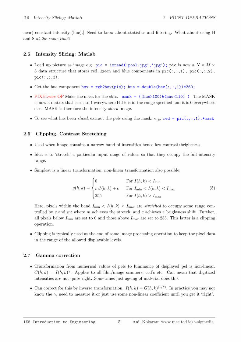
2.5 Intensity Slicing: Matlab

• Load up picture as image e.g. pic = imread(’pool.jpg’,’jpg’); pic is now a N ×M ×3 data structure that stores red, green and blue components in pic(:,:,1), pic(:,:,2),

pic(:,:,3).

• Get the hue component hsv = rgb2hsv(pic); hue = double(hsv(:,:,1))*360;

• PIXELwise OP Make the mask for the slice. mask = ((hue>100)&(hue<110) ) The MASKis now a matrix that is set to 1 everywhere HUE is in the range specified and it is 0 everywhereelse. MASK is therefore the intensity sliced image.

• To see what has been sliced, extract the pels using the mask. e.g. red = pic(:,:,1).*mask

2.6 Clipping, Contrast Stretching

• Used when image contains a narrow band of intensities hence low contrast/brightness

• Idea is to ‘stretch’ a particular input range of values so that they occupy the full intensityrange.

• Simplest is a linear transformation, non-linear transformation also possible.

g(h, k) =

0 For I(h, k) < Imin

mI(h, k) + c For Imin < I(h, k) < Imax

255 For I(h, k) > Imax

(5)

Here, pixels within the band Imin < I(h, k) < Imax are stretched to occupy some range con-trolled by c and m; where m achieves the stretch, and c achieves a brightness shift. Further,all pixels below Imin are set to 0 and those above Imax are set to 255. This latter is a clippingoperation.

• Clipping is typically used at the end of some image processing operation to keep the pixel datain the range of the allowed displayable levels.

2.7 Gamma correction

• Transformation from numerical values of pels to luminance of displayed pel is non-linear.C(h, k) = I(h, k)γ . Applies to all film/image scanners, ccd’s etc. Can mean that digitizedintensities are not quite right. Sometimes just ageing of material does this.

• Can correct for this by inverse transformation. I(h, k) = G(h, k)(1/γ). In practice you may notknow the γ, need to measure it or just use some non-linear coefficient until you get it ‘right’.


2.8 Image Histogram 2 POINT OPERATIONS

• I(h, k) = G(h, k)γ Matlab syntax: I =G.^0.5

• Matlab Demo: imadjdemo

• Adobe Photoshop allows you to do many different kinds of non- linear pixel mappings.

2.8 Image Histogram

An image histogram records the number of pixels which have a particular intensity value. Typicallyit is displayed as a graph showing the number of pixels that occupy each of a range of intensity values.It is often shown as a bar chart with the horizontal axis being the intensity values and the verticalaxis showing the number of pixels occupying each particular intensity ‘bin’. An image histogram istherefore just a bar chart showing the number of pixels that have a particular intensity or intensityrange. For an 8 bit histogram, the range of the horizontal axis would be typically 0 . . . 255 in stepsof unity. It is possible to have histogram using coarser ‘bin sizes’ for instance, 0− 4, 5− 9, 10− 14etc.

• Typically displayed as a plot of frequency Vs. intensity (or level, or value).

• Shows the distribution of intensities across the WHOLE image. Could be normalised so thatintegrates to 1 (an approximation of the Probability Density Function of the image intensities)by dividing by total pixels in image.

• Useful for working out where most of the information is and designing enhancement operations.

• Very useful for comparing images on the basis of overall ‘look’ or ‘feel’. Content retrieval onbasis of redness etc etc.

−50 0 50 100 150 200 250 3000

200

400

600

800

1000

1200

1400

Intensity

Fre

quen

cy

0 50 100 150 200 250 3000

2000

4000

6000

8000

10000

12000

14000

Intensity

Fre

quen

cy

2.9 Histogram Equalisation

• A powerful technique for image enhancement. But a bit of a loose cannon.

• Idea is to redistribute the assignment of intensities to the pixels in the image so that they areall equiprobable. Thus if image contains alot of information in a narrow band of intensities,this is stretched out over all the usable intensity range.

• See ppt. example


2.9 Histogram Equalisation 2 POINT OPERATIONS

• Problem is how to assign intensities to pels in the image. Got to choose! If you choose wrongyou could be making matters worse, and you can’t be consistent from image to image. UseCumulative Distribution to design mapping instead.

• Say image is N ×M pels. The p.d.f of an image with uniformly distributed pels will have aconstant value at 1

NM . This implies a Cumulative Distribution Function which is a straightline, having a gradient 1/256, a maximum of 1 and min of 0.

• Idea is now to transform the image intensities so that the CuF of the transformed imagematches the target CuF i.e. as close as possible to the straight line.

• Works for any target distribution. See ppt example.

• There is a quantitative proof (involving probability theory) that using the CuF will give theoptimal transformation for images with continuous grey scales i.e. analogue pictures. But thiswill not be covered here.

• Matlab function histeq.


2.9 Histogram Equalisation 2 POINT OPERATIONS

Left: Original image, Middle: Histogram Equalised Image, Right: Original Image ×1.2

−100 0 100 200 3000

1

2

3

4

5

6x 104

Intensity

Fre

quen

cy

−100 0 100 200 3000

1

2

3

4

5

6x 104

Intensity

Fre

quen

cy

−100 0 100 200 3000

1

2

3

4

5

6x 104

Intensity

Fre

quen

cy

Left: Histogram of Original image, Middle: Histogram of Equalised Image, Right: Histogram ofOriginal Image ×1.1

Left: Original image, Middle: Histogram Equalised Image, Right: Original Image ×1.1

−100 0 100 200 3000

200

400

600

800

1000

1200

1400

Intensity

Fre

quen

cy

−100 0 100 200 3000

200

400

600

800

1000

1200

1400

Intensity

Fre

quen

cy

−100 0 100 200 3000

0.5

1

1.5

2x 104

Intensity

Fre

quen

cy

Left: Histogram of Original image, Middle: Histogram of Equalised Image, Right: Histogram ofOriginal Image ×1.1

0 100 200 3000

2

4

6

8

10x 104

Intensity

CU

MU

LAT

IVE

Fre

quen

cy

0 100 200 3000

2

4

6

8

10x 104

Intensity

CU

MU

LAT

IVE

Fre

quen

cy

0 100 200 3000

2

4

6

8

10x 104

Intensity

CU

MU

LAT

IVE

Fre

quen

cy

Left: CUMULATIVE Histogram of Original image, Middle: CUMULATIVE Histogram ofEqualised Image, Right: CUMULATIVE Histogram of Original Image ×1.1


2.10 Summary 3 SPATIAL OPERATIONS

2.10 Summary

1. An image can be thought of as a matrix

2. There are some useful point wise or pixel wise operations for images that all are related to thefunction of scaling (contrast modification).

3. Histograms are useful for describing image content

4. Histogram modification can be used to perform non-linear image enhancement: HistogramEqualisation

5. These are very common image processing blocks. Often Pixel operations are assigned to specifichardware or software modules as they are used often.

6. Most of the pixel operations can be implemented as Look Up Tables since the input data istypically 8 bit. This is very important for fast, simple and reprogrammable moduledesign (whether hardware or software).

7. References

• Lim Pages 453–458

• Jain [Fundamentals of Digital Image Processing] Pages 235–244

3 Spatial Operations

Images are by their nature spatial processes It is sensible that more useful effects can be achievedby treating groups of pixels together. This section covers the following ideas

1. Masks and filters: averaging, weighted average

2. Masks and filters: differencing, weighted differencing

3. The Median Filter: A Non-Linear Filter

Note that the ideas discussed here are founded in sound principles of filter design and signalprocessing which you will meet in your 3rd year. In this course the idea is not to give you all thedetails, just enough for you to get a feel for what these things can be used for.

3.1 Averaging filter

• We will consider one type of filter : Finite Impulse Response (FIR) filters that can be moreeasily visualised through the use of a convolution mask.

• In general the output of a 2D averaging filter can be written as

g[h, k] =1

NM

M∑

m=−M

N∑

n=−N

I[h + m, k + n]


3.2 Weighted Average 3 SPATIAL OPERATIONS

Output depends on pixels at the current site as well the neighbourhood of that site. Thosepixels are all around the current site.

• To solve this difference equation for g1(·) we need I(h, k) (of course), but we also need BOUND-ARY conditions at all boundaries of the input I(h, k).

• In other words to process I(h, k) with this filter, we really ought to know the values of I(h, k)everywhere.

• In practice we need to assume some kind of boundary conditions at image edges.

• Rather than thinking of the filtering operation as arising from equation 6; it is convenient tothink of it as filtering the image with a geometric shape that has different weights for each pel:a filter mask.

Odd sized masks

−1−1 4 −1

−1

1 1 11 1 11 1 1

× 1

9

• Output value at a site is calculated by positioning the ‘centre’ of the mask over the site. Thenthe products between the various mask weights and the corresponding pels in the input imageare calculated and summed to give the output of the system at that site.

3.1.1 Manual Example

Calculate the output image when the image below is filtered with a 3× 3 averaging filter. State anyboundary conditions you assume.

10 10 20 10 1010 10 20 10 1020 20 20 20 2010 10 20 10 1010 10 20 10 10

3.2 Weighted Average

A weighted average filter is a generalisation of the averaging idea. These are low pass filtersbecause they remove the high frequency content in an image. Edges and texture generally representthe high frequency content in images. Hence they are attenuated by this kind of filter. Low passfilters therefore BLUR an image because they REMOVE image detail.

In order for these filters not to affect the average brightness of an image, theircoefficients must sum to UNITY. Understand this by thinking about what would happen if youfilter a flat picture with this kind of filter.



1 2 12 4 21 2 1

× 1

16

0.0125 0.0264 0.0339 0.0264 0.01250.0264 0.0559 0.0718 0.0559 0.02640.0339 0.0718 0.0922 0.0718 0.03390.0264 0.0559 0.0718 0.0559 0.02640.0125 0.0264 0.0339 0.0264 0.0125

A popular low pass filter for images is the GAUSSIAN filter, which is derived from the Gaussianexpression.

f(x) =1√

2πσ2exp

(−x2

2σ2

)

The filter on the right above is a Gaussian filter. The images below show the mask of an 11× 112D Gaussian filter with σ2 = 4.

02

46

810

12

0

2

4

6

8

10

120

0.01

0.02

0.03

0.04

0.05

0.06

0.07

0.08

1 2 3 4 5 6 7 8 9 10 111

2

3

4

5

6

7

8

9

10

11

What would the contours of an Averaging filter look like?


Calculate the output image when the image below is filtered with the filter having a mask as follows.

1 2 12 4 21 2 1

× 1

16

State any boundary conditions you assume.

10 10 20 10 1010 10 20 10 1020 20 20 20 2010 10 20 10 1010 10 20 10 10

3.2.2 Pictures

To process pictures with these filters you would have to write some computer program because thereare too many pixels for you to be doing this automatically. In Matlab there is an in-built functioncalled conv2 that does this for you.



Top: Original Lenna, Filtered with Gaussian filter 21× 21 mask, σ2 = 1,Difference g[h, k]− I[h, k] + 128 (shifted by 128 so that mid- gray is zero)

Top: Original Lenna, Filtered with Gaussian filter 21× 21 mask, σ2 = 42,Difference g[h, k]− I[h, k] + 128

Top: Original Lenna, Filtered with Average filter 11× 11 mask,Difference g[h, k]− I[h, k] + 128

The averaging filter is not a very good image blurring filter.


3.3 Separable Filters 3 SPATIAL OPERATIONS

3.2.3 Computation

• Say we have a filter mask with R × C taps, and a N × M input image. At each site tocalculate the output we need to do R × C multiply/adds [= 1 instruction on most modernDSPs]. Therefore assuming a MADD is 1 operation, using this mask requires N ×M ×R×C

operations. This could be huge if the mask is large.

• A largeish low pass filter can be say 11×11 taps, so lets say you were processing video data at576× 720 pels per frame with 25 frames per second. Then that’s 414720× 11× 11 ≈ 50Mops

per frame. This means about 50× 25 = 1.2Gops per second for TV. A Texas Instruments C60could probably just not do this as it can give at most 1Gop. But recent C60’s at higher clockrates probably could.

• FPGA and IC designs however, can achieve these rates.

• Filter building blocks are quite important for real time image/video processing.Hence general purpose processors like Pentia, ARM and even DSPs like C6x and TriMedia allattempt to include architectures which can achieve ‘real time’ performance for these blocks byusing VLIW and even wider data paths/pipelines.

• Several research laboratories around the world are now looking at Graphics Processors inMobile Phones for filtering images....

• Remember Real Time is a very subjective thing. When people say ‘We can do “blah-blah” inreal time’, you need to know what the input data rate is before you can really appreciate theclaims being made. I could say that a 300 MHz pentium can do filtering with a 11× 11 filtermask, and histogram computation and scene cut detection in real time for video1. But if youask “What are the size of the processed images?” The answer would be 176× 1442 (approx).

3.3 Separable Filters

• It turns out that some filters can be implemented by cascading TWO operations using 1-DFILTERS!

• These are called Separable Filters and they are implemented by filtering along rows then alongcolumns (or vice-versa, it does not matter).

•

Using

1 2 12 4 21 2 1

× 1

16(6)

Is the same as[

1 2 1]× 1

4followed by

121

× 1

4(7)

1This is true.2This size of image is called QCif in the image processing industry



• Really useful if you can spot that your 2D filter is separable since you can reduce computationenormously. Computation for a cascade of a row and column filter with sizes R and C tapsrespectively is N ×M ×R+N ×M ×C = N ×M × [R+C]. For 11×11 example computationis reduced by a factor of 5 !!

NMRC

NM(R + C)=

12122

= 5.5 (8)

Now you can definitely do the filtering in real time for TV on a C60. If the filteringoperation is separable.

• Gaussian Filters can be implemented in a separable fashion.

3.3.1 Check if you understand

The filter mask below is separable using the same 1-D filter along rows and columns. What is the1-D filter?

0.0048 0.0595 0.00480.0595 0.7432 0.05950.0048 0.0595 0.0048

3.3.2 Noise and Noise Reduction

Low Pass filters are useful for removing noise in an image. Noise is found in most images recordedusing some measuring apparatus. The value of the noise at a particular pixel is a random variable.It cannot be known exactly. It is only possible to say that the value of the noise at a particularpixel is for instance, 5, with a particular probability. We can write many kinds of noise corruptionas follows.

g[h, k] = I[h, k] + e[h, k] (9)

where we say that e[h, k] is drawn from a particular probability distribution pe(e). The look andfeel of the noise depends on this probability distribution as well as the correlation in the noise. Herewill assume that the noise is uncorrelated. This means that the noise value at one pixel does notinfluence the noise value at a nearby pixel. This is not true for film grain noise, where the noise iscorrelated because of the image formation process there. Uncorrelated noise is a pretty good guessfor Digital Cameras in general.

The pictures below show Lenna corrupted with additive noise where e[h, k] is zero mean anddrawn from a Gaussian Probability Density Function as follows.

pe(e = x) =1√2πσ2

e

exp(

x2

2σ2e

)(10)

For a Gaussian distribution, there is a shorthand for writing this which is e[h, k] ∼ N (0, 100). TheN stands for Nnormal Distribution (Gaussian is Normal). The first argument is the mean and thesecond is the variance of the random variable e[h, k].



Left to Right: Original Lenna, e[h, k] ∼ N (0, 100) shifted by 128 so mid-gray is zero,g[h, k] = I[h, k] + e[h, k]

−100 0 100 200 3000

200

400

600

−50 0 500

1000

2000

3000

Left to Right: Original Lenna Histogram, Histogram of e[h, k] ∼ N (0, 100)

To give some idea of how badly corrupted an image is, we can use the Peak Signal to Noise Ratiowhich was defined in the previous handout as

PSNR = 10 log10

(2552

1NM

∑k

∑h(g[h, k]− I[h, k])2

)(11)

PSNR is measured in dB. For the corrupted image above, the PSNR is 28 Decibels or 28 dB.

The pictures below show corruption with three different noise levels again where the noise isGaussian and independent.

Corrupted versions of Lenna with additive Gaussian Noise Left to Right: e[h, k] ∼ N (0, 10) PSNR= 38 dB, e[h, k] ∼ N (0, 100) PSNR = 28 dB, e[h, k] ∼ N (0, 1000) PSNR = 18.1 dB



If one picture has a higher PSNR than another, is its relative picture quality worse or better?Why?

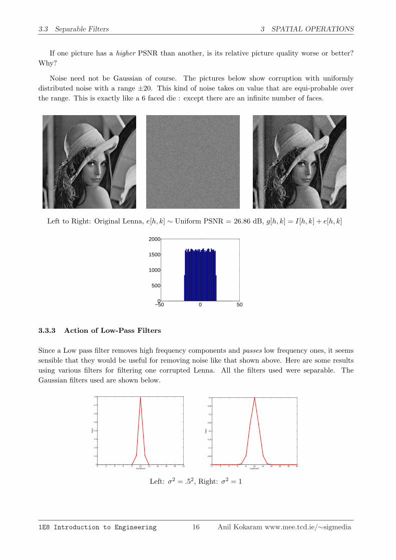
Noise need not be Gaussian of course. The pictures below show corruption with uniformlydistributed noise with a range ±20. This kind of noise takes on value that are equi-probable overthe range. This is exactly like a 6 faced die : except there are an infinite number of faces.

Left to Right: Original Lenna, e[h, k] ∼ Uniform PSNR = 26.86 dB, g[h, k] = I[h, k] + e[h, k]

−50 0 500

500

1000

1500

2000

3.3.3 Action of Low-Pass Filters

Since a Low pass filter removes high frequency components and passes low frequency ones, it seemssensible that they would be useful for removing noise like that shown above. Here are some resultsusing various filters for filtering one corrupted Lenna. All the filters used were separable. TheGaussian filters used are shown below.

0 2 4 6 8 10 12 14 16 18 200

0.1

0.2

0.3

0.4

0.5

0.6

0.7

0.8

Coefficient

Val

ue

0 2 4 6 8 10 12 14 16 18 200

0.05

0.1

0.15

0.2

0.25

0.3

0.35

0.4

Coefficient

Val

ue

Left: σ2 = .52, Right: σ2 = 1



Left to Right: Corrupted Lenna PSNR = 28dB, Filtered with 21 tap Gaussian filter; PSNR=30.5dB, g[h, k]− I[h, k]

Left to Right: Corrupted Lenna PSNR = 28dB, Filtered with Gaussian filter (σ2 = 1.52)PSNR=27.8dB, g[h, k]− I[h, k]

Left to Right: Corrupted Lenna PSNR = 28dB, Filtered with 9 tap Average filter PSNR=24.8dB,g[h, k]− I[h, k]

Does this result really look good? Is anything wrong? What can be done to improve this kindof noise reduction operation?

It turns out that to do a really good job of noise reduction, you have to incorporate the knowledgeof the statistics of the noise in your algorithm. Since in this case we know the p.d.f. of the noise, and


3.4 The Median Filter 3 SPATIAL OPERATIONS

we can make some assumptions about the original image, it is possible to derive an optimal filterto remove noise. One of the simplest filters of this kind is called the Wiener filter. Its a bit trickyto explain, but it exploits the frequency domain to work its magic. Even then the result isn’t thatgreat and some further intuition has to be applied to get very good pictures. The pictures belowshow the result of noise reduction when this kind of special optimal, adaptive filter is used.

Noisy Lena PSNR=28dB Wiener Filter result Gaus. 11 tap, σ2 = 1.5

3.4 The Median Filter

The Median filter is very useful in image processing for treating impulsive distortion. Idea is todefine some N × N filter geometry and then the output of the filter is the median of the pixels inits window.

It was invented in the 60’s by a guy called Tukey. He used it for smoothing out the data fromseismic surveys. For a simple filter it is surprisingly effective.

Given the image below, work out the output when a median filter with a 3× 3 window is used.


3.4 The Median Filter 3 SPATIAL OPERATIONS

10 10 20 10 1010 100 20 10 1020 20 20 0 2010 0 20 255 1010 10 20 10 10

10 10 20 10 1010 100 100 100 1020 100 100 100 2010 100 100 100 1010 10 20 10 10

Left to Right: Lenna corrupted with Impulsive noise, Filtered with 5×5 median filter, Filtered with5× 5 average filter

Why does the median filter remove impulsive noise well? Does it damage any of the underlyingimage detail?

• Problem is that median filter preserves gross image edges but ejects fine texture. Causes akind of flattening of detail.

• This filter is one from the class of Order statistic filters. The output of this general class issome kind of statistic measure of the pels in its window e.g. Upper Quartile, Lower Quartileetc. Need to calculate histogram of pels in the window then select the pel at Q1 or Q3 etc.

• Around 1990 a few researchers (Arce et al) spotted that you could improve the performanceof the median operator by cascading filter geometries. These are called multistage medianfilters.


3.5 Differencing and Gradients 3 SPATIAL OPERATIONS

Median

� ��

� ��

� ��

� ��

� � ��

� � ��

� � ��

� ��

� ��

� ��

� ��

� ��

� ��

� ��

� ��

� ��

� �� 14

14 14

14

3

15

200

101

Median filter output = 14

Median Median Median

Many people have studied these kinds of filters, and in the late 1990’s they were extended foruse in video and film. Those structures are now being used in the film and video industry.

3.5 Differencing and Gradients

If we define the spacing between each pixel to be unity, then the horizontal gradient at each pixelin an image can be calculated with

gx[h, k] = I[h, k]− I[h− 1, k]

and the vertical gradient isgy[h, k] = I[h, k]− I[h, k − 1]

This is the same as filtering with a filter having a mask [−1, 1] and [−1, 1]T respectively

These kinds of filters are known as High Pass filters because they attenuate or suppress LowFrequency information. See the examples below to see how this is so. They can be used to enhancedetails in an image.


Calculate the output image when the image below is filtered with gradient filters [−1, 1] and [−1, 1]T

State any boundary conditions you assume.

10 10 20 10 1010 10 20 10 1020 20 20 20 2010 10 20 10 1010 10 20 10 10



3.5.2 Pictures

Left: Original Mayaro, Filtered with [−1, 1], Difference g[h, k]− I[h, k]

Left: Original Mayaro, Filtered with [−1, 1]T , Difference g[h, k]− I[h, k]

3.5.3 Edge Detection

We can use the gradient filters above to detect edges in an image. This is important for imageanalysis e.g. object recognition, face detection. The simplest method is simply to define edges asthose image features having large gradient magnitude gmag.

gmag[h, k] =√

gx[h, k]2 + gy[h, k]2 (12)

Thresholding this magnitude yields edges.



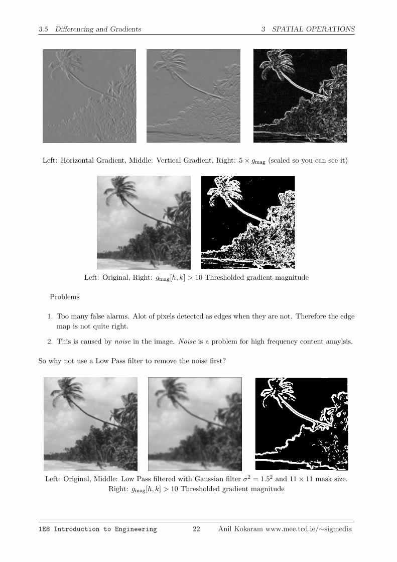
Left: Horizontal Gradient, Middle: Vertical Gradient, Right: 5× gmag (scaled so you can see it)

Left: Original, Right: gmag[h, k] > 10 Thresholded gradient magnitude

Problems

1. Too many false alarms. Alot of pixels detected as edges when they are not. Therefore the edgemap is not quite right.

2. This is caused by noise in the image. Noise is a problem for high frequency content anaylsis.

So why not use a Low Pass filter to remove the noise first?

Left: Original, Middle: Low Pass filtered with Gaussian filter σ2 = 1.52 and 11× 11 mask size.Right: gmag[h, k] > 10 Thresholded gradient magnitude


4 SUMMARY

4 Summary

In this section we have dealt with the following

• 2D FIR Filters and their implementation as Filter Masks

• Implementation and speed

• Noise and noise reduction with filters

• Relating dB to image appearance

• Gradient filters and edge detection

• The Median filter


1e8: introduction to engineering introduction to image …ack/teaching/1e8/lecture2.pdf · 1e8:...

Documents