'. fMAXTR-76-11 I, Vol I (of sev4n9)

W APPLICATIONS OF .iaw MXsM W YNW SvIC LZ1E 7HEORY

C44TOTHEFRICTONOFCABLE fC(MJ~W~

O ~ýUjticondutctr Traissmisslon Linec Theory

I A~~~pqr~ fo,,, public riae

1'A004MMCR

GRO AM FOW W-4iVFW YSmI13441RlEPRODUCED BY

NATIONAL TECHINICALI : ONFORMAMIN SERVICE

IUls bpncha bees rr-lad by cbms UIt'C lforustlo Of fiaz (01) jagis rlsasibis to the matcta.r- %tedchnal InfrruionsService WU i AtnTII,,* will be nolsmt I*e to the gin&Inl public tacludins foreign mastlos.

This rupprr has be.. rsflmsid ad is approved for' pubiS -Fiton.

JAM0 Cx. sauurr

Alef. IJMAtfliy &Camecibitiy Dtutstoc

Pt IST CSMBM fl: 2. -Ze

Po not tetlkrn 04_44v ,-opy Ma sia or &osLitc1,

SMACURITY CLASSIrt'.AION OF THIS 04PJ% (When D08g Ruldtld)_______________________

REDINSTRUCTIONSREPORT DOCUMENTATION PAGr,, 827FORE COMPLETING FORMoff. REkN JUM aUA - - Q4 ACC~FSSION NO- I- I'~T CATALOG NUMBER

RADC-TR--76-lO1, Vol I (of seven) ---i______4. TiTLi fad SUhelule.) i. T7%:v FSP ~P9T&P~APPLICATIONS OF MULTICONDUCTOR TRANSMISSION LIINE Final Technic,7, ReportTHEORY TO THE PREDICTION OF CABLE C3UPLING ______________

Vol I -~ Multiconducror Tranooission Line Iteory 0. PERFORMIN4G ORG. RERCIRY NUMUEPn

____ ____ - __ ____ ____ ___ N/AV. AUTHOReo) -U.COi 1RACT ORGRXN-YNjIM0EERI

Clayto.i R. Paul F30602--72-C--0418

T. -PERFORMING ORGANIZATIOtJ NAS.IE AND ADDRESS tO rpczGPAM ELEMEN4T. PROJECT, TASKAREA A WORK UNIT NUMIRFRS

D.,iversity of KentuckyDepartment of Electrical Engineering 62702FLexington ICY 40506 45400130 ____

11. CONTROLLING OFPICIK NAME AND AD0111511 12. REPORT DATE-

April 1976Rome Air Development Center (RBCT) 13. NIUMSIFP OW PAGES

Grif fiss AFB NY 13441 _________ 23r4F. NMOr~ffTORING AGENC~Y N.AME & ADDR183(ti'iEIIoret from, Conltrol~ling Office) .. SECURITY CLASS. (ofteeol

Same UNCLASSIFIEDI E(.a-. DL!3IICATiOcN7aiOWNOIRADitNO

* Ii" G1STVr-IuTION STATEMAENT (of this flewit)N/

Approved for public release; distribution unlimited.

PKsSWBJL"IE TO CHAN'GEE17. DISTAIR U T~o T o h btatonodi lv 0 dhiseuUt howl Roepot)

Same

WS SUPPLEMENTAR'Y NOTES(

RADC Project Engineer: James Brodock (RBCT)

1S. KEY WORDS (Contirnua on revevsidea itd lnave##" and ld-..ulf' ky block .anumber)

Electromagnetic Comnpatibility Wire-to-wire CouplingCable Coup]ling Rlbbon CableTransmission Lines Flat Pack CebleHulticonductor Transmission lines

ao.A9ZTRACTW(C, 111nuW-a itS nIe Ufamacmv and hft*nt fty -hy blook mornbor)

This report io the firat volinmo in a series of reports documenting theApplicntion of Multiconductor Transmission Line Theory to the Prediction of

K Cable Coupling. Modern avionics systems are becoming increasingly complex.Thece systems generally contain large numbers of wires connecting the variouselectronic equipr-santo. Thie T,2jority of the wirc are in very close proxiLmity

L to each other in ebither random cabla bundle6 (in which the relative wirepoitiono are not known or controlled) or in ribbon cables (in which the

DI 1473 IO umyl .7 C'3OV0, a@ is UNCLASSIFIED9E0CUtnT'V CLASSi iATIOU OP T"ItS PArif (WThen Date Enteralf,

UNCLASS IFIEDSECUR17Y CLASSIFICATION OV THIS PAGCrW?,W Dpat £nrat )______________________

Stelative wire positions are known and controlled). The prediction of oire-coupled interference in these cable bundles is of considerable importance in6h9 prediction of overall system compatibility. It in the purpose of thioseries of reports to examine the application of multic3nd:ctor trausminoionline theory to this problem.

Thi first volume is intended to provide a com?rehensive discusnion ofmulticonductor transmission line theory on which the remaining volumen willbe based. The remaining volumes will investigate the application of thistheory to specific classes of problems. Considerable experimental. verificationwill be included in the later volumes to indicate the degree of confidencewhich can be placed in these models when they are applied to specific situations

Vol%ýmes I, II, and III have been completed at this time and Voluie IVis iv pqeýaration. Other volumes covering shielded wires, twisted pairsand ter:inal currents induced by external incident fields will be included.The completed volumes and thoseo in preparation are:

Volume I MiULTICONDUCTOR TWISMISSION LINE THEORY

Volume II COMPUTATION Or THE CAPACITANCE MATRICES FOR RIBBON CABLES

Voltuae III - PREDICTION OF CROSSTALK IN RAbj 'M CABLE BUNDLES

Volume IR - PREDICTION OF CR'OSSTALK IN RIBBON CABLES

UNCLASSIFIrD

SFCU-ITY CLASSIFICATIOnt 01C Yt4jS PAG'f1,on biw enter'od)

PREFACE

The Post-Doctoral Program at Rome Air Development Center is pursued viaProject 9567 under the direction of Mr. Jacob Scherer. The Post-Doctoral

Program is a cooperative venture between RADC and the participating univer-

sities: Syracuse University (Department of Electrical and Computer Engineer-

ing), the U.S. Air Force Academy (Department of Electrical Engineering),

Cornell University (School of Electrical Engineering), Purdue University

(School of Electrical Engineering), University of Kentucky (Department of

Electrical Engineering), Georgia Institute of Technoloqy (School of Electrical

Engineering), Clarkson College of Technology (Department of Electrical

Engineering), State University of New York at Buffalo (Department of Electri-

cal Engineering), Korth Carolina State University (Department of Electrical

Engineering), Florida Technological University (Department of Electrical

Engineering), Florida Institute of Technology (College of Engineering), Air

Force Institute of Technology (Department of Electrical Engineering), and the

Universitý of Adelaide (Department of Electrical Engineering) in South

Australia. The Post-Doctoral Progr~m provides, via contract, the opportunity

for faculty and visiting faculty at the participating universities to sp -nd

a year full-time on exploratory development and operational problem-solving

efforts with the post-doctorals splitting their time between RADC (or the

ultimate customer) and the educational institutions.

The Post-Doctoral Program is totally customer-funded with current

projects being undertaken for Air Defense Comnmend (NORAD), Air Force Communi-n

cations Service, Federal Aviation Administration, Defense Commuinications

Agency, Aeronautical Systems Division (AFSC), Aero-Propulsion Laboratory

(AFSC), and Rome Air Development Center (AFSC). This effort was funded by

Rome Air Development Center Electromagnetic Compatibility Branch under

Project 4540, Contract F30602-72-C-0418.

Clayton R. Paul received the BSEE degree from the Citadel (1963),

the MSEE degree from Georgia Institute of Technology (1964), and the PhD

degree from Purdue University (1970). He served as a graduate assistant

(1963-64) and as an instructor (1964-65) on the faculty of Georgia Institute

of Technology. As a graduate instructor at Purdue UJ,,verbiLy (1965-70) he

taught courses in linear system theory, electrical circuits and electronics.

From 1970-71 he was a Post Doctoral Fellow with RADC, working in the area I

of Electromagnetic Compatibility. His areas of research interests are in

linear multivariable systems and electrical network thscory with emphasis

on distributed parameter networks and multiconductor transmission lines.

9

ii

I

TABLE OF CONTENTS

PAGE

I. INTRODUCTION ----------------------------

I1. THE TEM MODE FORMULATION FOR

MULTICONDUCTOR LINES 5--------------------5

III. SOLUTION OF THE TRANSMISSION LINE EQUATIONS ----- 31

3.1. Transmission Lines ina Homogeneous Medium ------ 483.2. Transmission Lines in Inhomogeneous Media----- --- 533.3. Cyclic-Symmetric Matrices,5 -...... -- --- 56

IV. INCORPORATING THE TERMINATION NETWORKS--- - - ---- 61

4. 1. Lumped-Circuit Iterative Approximations - ----------- 69

V. THE PER-UNIT-LENG'..i PARAMETERS -----------. - ------ 82

5.1. The Per-Unit-Length External Parameters for

Lines in a Homogeneous Medium----------------- ---- 835.2. The Per-Unit-Length External Parameters for

Lines in an Inhomogeneous Medium ---- - ------------- 101

VI. SUMMARY - ---------------------------------------------- 123

APPENDIX A- - ------------------------- --125

APPENDIX B----------------------------------------- ----130

APPENDIX C- - ------------------------ ----133

APPENDIX D- - ------------------------ ----157

APPENDIX E- ------------------------------------------ 163

REFERENCES ------------------------------------------- 169

iii

LIST OF ILLUSTRATIONS

FIGURE PAGE

1. An (nil)-conductor uniform tranlsmission line.

Sheet 1 of 2 .........-.............-- ------------------- 6Sheet 2 of 2 ........- ...........-- ----- ---------------- 7

2. Multiconductor transmission lines in a homogeneoua medium- - _ 12

3. Multiconductor transmission lines inan inhomogeneous medium.

Sheet I of 2 -- ------------------------------------------------- 13Sheet 2 of Z -. ------------------------------------------------- 14

4. Two-conductor t'ansmission lines in a homogeneous medium. 15

5. Two-conductor transmission lines in an inhomogeneous medium.Sheet 1 of 2 -------------------------------------------------- 16Sheet 2 of 2 -------------------------------------------------- 17

6. The termination-networks and equivalent

circuits for two-conductor transmission lines.Sheet 1 of 3 -------------------------------------------------- 20Sheet 2 of 3 -- - - - - - - - - - - - - - - - - - - - - - - - - - - - -21

Sheet 3 of 3 - - ----------------------------------------------- 22

7. The per-unit-length equivalent circuit for multiconductortransmission lines .-- ---------------------------------------- 23

8. Cyclic-symmetric structures -------------------------------- 57

9. The termination-networks for multiconductor transmission lines -62

10. The termination-netkvorks for multiconductor transmission lines -64

11. Lumped-circuit iterative models of multiconductor transmissionlines.

Sheet 1 of 4 -------------------------------------------------- 71Sheet 2 of 4 ........---------------------------- --- 72Sheet 3 of 4 -------------------------------------------------- 73Sheet 4 of 4 -------------------------------------------------- 74

12. The geometry of the charge distribution problem--------- --- 86

iv

FIGURE PAGE

13. Multiconductor transmission lines above a ground planeand the use of image distributions. - - - --------------------- 93

I,'. The replacement of the wires and the shield with infinitesiLial

line charges for shielded, n-.ilticonductor lines with largeseparations in homogeneous media. W-00

15. The geometry for Table I. - - ------------------------------ 104

16. Computed results for two dielectric-insulated wires.--- - - --- 107

17. Computed results for a five-wire ribbon cable.----- 109 A

18. Dielectric-insulated wires above a ground planeand the image distributions- - ---------------- -- ---- 0

19. A two-wire line and the selection of the match noints. -l-- -113

20. A two-wire line above a ground plane and the

selection of the match toints.-- --- ----------- ---- - -- 118

GC-I. A multiconductor line with incident field illumination ------- 134

C-2. The per-unit-length equivalent circuit for Fig. C-I. --------- 135

C-3. The problem geometry for the calculation of the entries Iin the per-unit-length inJuctance matrix -------------------- 149

C-4. The geometry for the example.- - ------------------ 152

C-5. Multiconductor lines above a ground plane. - - -------------- 155

E-1. The geometry for the derivation of the potential expression,. - -164

vI

*i

IVt

I. INTRODUCTION

Coupled tran, inission lines have continually rec,-ived much attention in

many diverse areas of application. Multiconductor transmission lines have

been investigated in early power system studies and continue to receive

attention in this area with regard to the transient behavior of power lines

under fault and lightning induced conditions [1-13]. Modern emphasis on

multilayer distributed circuits, strip lines and microstrip associated with

integrated-circuit technology has produced e renewal of interest [14-19, 68]

as has the interest in predicting transients induced on cables by external

electromagnetic field sources such as high power radars or an electromag-

netic pulse (EMP) from nuclear detonations [20-27]. Determining cross-

talk in communication circuits [28-30] and digital computer wiring inter-

ference [30-32] are examples of other areas in which the subject of multi-

conductor transmission lines consistently arise.

Of particular interest within the electromagnetic compatibility (EMC)

community is the prediction of coupling between wires and their associated

termination-networks in c]osely coupled, high density cable bundles and

flat pack (ribbon) cables on modern electronic systems. Control of intr,*-

system electromagnetic compatibility for systems within the Department of

Defense is generally governed by MIL-STD-461 and 462. These are general

documents which prescribe limits on emissions and susceplibilities of the

individual subsystems and equipments with regard to undesired signals

(interference) and do not in themselves consider the coupling paths between

C -1-

the equipments and subsystems within systems. The undesired signals as

used in this context are with respect to the particular equipment or sub-

system, not all , which are undesired from the overall system standpoint.

For example, the undesired signals may be truly undesir.•d ones, such as

transmitter harmonics, or may be the result of an essential signal, such as

the fundamental frequr, t of a transmitter, coupling to a receptor for which

such coupling is not intended.

Even if all the equipments and subsystems within a system conform to

the limits in MIL-STD-461, it is, of course, not necessarily true that over-

all system compatibility will be achieved. Since these limits do not take

"I into account the various coupling mechanisms and proximities of the equip-

ments, a systen whose equipments and subsystems meet ML-STD-461 may

prove to be incompatible and numerous instances of required retrofit and

interference suppression measures on systems meeting these lirnits illus-

trate this fact. Thus overall ,;ystem compatibility may not l:Ie achiev'ed

unless all signals (d~esired and undesired) and actual coupli'rg paths within

A• the system are considered, analytically. This deficiency has led to the

development of various computer-aided intra-systern (as :,pposed to inte.-

system) cormpatibility prediction programs which mathen',atic lly model the

systems and take into accotut the various coupling path, for unintentional

energy transfer (interference) as well as intentional energy transfer [33. 31],.

The various coupling paths can generally be classified into combina tions

of wire, antenna and raetallic box coupling, e.g., wire- to-wire, anterm.a-

) :i•'ff•• •':~~~~~~~~~~~~~~~~.... :•''..............::4' i• ..... ' • •- • -... .. •. • iJ.•. • •J.ki

S to-antenna, antenna-to- wire, box-tL -box, etc. In the case of wire-to-wire

coupled interference in cable bundles, this undesired coupling of energy

between circuits sharing a common bundle may be more severe than one

rnaý eaiize. For example, numerous cases (both experihlental and analyti-

cal) may be shown where, for certain frequencies, the ratio of the received

interference voltage across the terminals of a device to the voltage emitted

by another device, which is coupled -via wire-to-wire coupling mechanisms,

exceeds unity. The two devices are not directly connected by a common

pair of wires; the wires connected to each device are only in close proximity

in a common cable bundle. Rarely does one encounter voltage transfer

functions with magnitudes greater than unity in antenna-to-antenna inter-

ference coupling problems and this illustrates the importance of considering

the mechanism of wire-coupled interference transfer.

It is the purpose of this report to provide a co.nplete -- id unified discus-

Ssion of multiconductor transmission line theory as it applies to the predic-

tion of wire-coupled interference. The common approaches and assumptions

which are either explicitly or implicitly used in the problem formulations

which appear throughout the literature are discussed. In addition to provid-

ing a discussion of the limitations and advantages of each of these techniques,

some numerically stable and efficient techniques for solving the multicon-

ductor tranumission line problem for large numbers of closely coupled,

dielectric-insulated wires will be presented. Methods for computing the

per-unit-length parameters will also be given. Some of the results can be

-3-

Ifound in various places in the literature although the treatments of the sub-

ject of multiconductoor lines generally either discuss the solution of the

equations describing the transmission line and associated termination-net-

works with the entries in the transmission line equations (the per-unit-length

parameters) assumed to be obtainable or they discuss the derivation of the

per-unit-length parameters without regard to the solution of the equations

describing the line. The purpose of this report is to provide a comprehen-

sive discussion of the complete problem solution and in addition present

sonme new techniques for considering large numbers of closely coupled,

dielectric-insulated wires.

Throughout this report, the emphasis will be on the frequency respons-e

of the transmission lines rather than the transient response since EMC con-

trol documents currently apply predominantly to the frequency domain. If

one assumes linear termination networks (no hysteresis, etc.) and assumes

no nonlinear effects associated with the transmission lines such as corona

discharge, then the equations describing the problem (the transmission lines

and associated terminations) will be linear and thus the freque.-cv response

provides a comr~etely general characterization.

Mlatrix formulation of the equations and other results of matrix analysis

will be used where necessary for a logical and concise development and the

reader is referred to [38) or other texts on linear algebra listed in the refer-

ences.

-4-

S I•II. THE TEM MODE FORMULATION FOR MULTICONDUCTOR LINES

I

Consider a Ax length section of an (n+l)-conductor, uniform transmis-

sion line in a homogeneous medium shown in Fig. 1 lying parallel to the x

direction in a rectangular coordinate syetem. The line is said to be uniform

if there is no cross-sectional variation with x either in the conductors or the

characteristics of the mediurm, i.e.. "end-on" or' crosL- sectional views in

planes perpendicular to x are identical for all x. The medium surrounding

the conductors and contained within the zero-th conductor is assumed to b,

linear and isotropic and therefore is describable by the scalars e (permit-

tivity), U (permeability), and a (conductivity) which are independent of the

electric and magnetic fields in the medium but may be functions of frequency.

If e, u and a are independent of position in the medium, i.e., independent of

x, y and z, the medium is said to be homogeneous. Thus for uniform lines,

all (n+l) conductors have uniform cross sections along their lengths and are

parallel to each other and the x direction and in the case of an inhorno-

geneous medium, the characteristics of the medium (e, L1, a) exhibit no

cross-sectional variation with x and are therefore independent of x.

The conventional distributed-parameter, transmission line model, of

course, describes only the TEM (Transverse Electro-Magnetic) mode of

propagation on the line and higher order modes are not considered. The

-4elec-tric £ield intensity vector, e (x, y, z, t), and the magnetic field intensity

vector, X ýx, y, z, t), for the TEM mode of propagation both lie in planes (y, z)

transverse or perpendicular to the direction of propagation (the x direction)

0 ,-

lel

I _

Figure 1. An (n+1)-conductor uniformtransri iission line (cont..

I~1. -

y

( b)

J (X,t) 0

0 0V ' (X,t) 0 1(4t

iS

?fOx(0) 0

x x+&x

r-igure 1. An (n+l)-conductor uniformtransmission line.

-7-

and t is the time variable. Thus it has been shown a number of times that,

assuming (n+l) perfect ccnductors, a homogeneous medium and the TEM ' Imode of propagation, the nouzero components of the field vectors (the trans..

verse electric field, eT(x, y, z, t), and the transverse magnetic field,

XT(xy, z, t)) at each x along the line satisfy the same spatial distributions as

static fields [40]. Therefore one can meaningfully define voltages between II

the conductors and currents flowing on the conductors [40]. For further

clarification, see Appendix A.

The emphasis in this report will be upon determining the frequency

response of the transrrdssion lines and associated termination-networks.

Therefore sinusoidal excitation is assumed with the field vectors written as

P(x, y, z, t) = E(x, y, z)eJ(ot and X(x, y, z, t) = H(x, y, z)e where E(x, y, z) andH(x,y, z) are complex-valued vectors independent of time t and w is• the

radian frequency of excitation ( = 2rr if). To characterize lines in a homo-

geneous medium such as in Fig. 1 under the TEM mode assumption, the

potentialYr(x, t), of the i-th conductor with respect to the reference con.-

ductor (the zero conductor) and the current, Ji(x, t), associated with the

i-th conductor are defined for i=l,--,n (see Fig. Ic). The currents are

directed in the positive x direction and t:.e current in the reference conduc-

ntor satisfies J0 (x, t) = - 4 i(x, t) [40]. Voltages and currents for- sin-

i;1

usoidal excitation aze written asl/0(x, t) = Vi(x)eJWt and J.(x t) = li(x)eJu)t

where Vi(x) and Ii(x) are the phasor voltages and currents respectively and

are complex-valued scalars independent of time, t. In the cross-sectional

-8-

ri

view of Fig. lb. the voltage of the i-th conductor with respect to the zero-th4l

conductor chosen as a reference is defined as the lir' integral of P T along

contour Ci in the y, z plane ard the current associated with the i-th conductor

+ Ais defined as the line integral of N T along the closed contour Ci in the y, z

plane. The assumption of TEM rgode propagation precludes the existence of

cornponent of the magnetic field intensity vector in the longitudinal direc-

tion (the x direction). This assumption coupled with the assumption of per-

fect conductors insures that the definition of the voltagcd is unique [40]. The

assumption of a rEM fields structure also precludes the existencz of a longi-

tudinal component of the electric field intensity vector. Therefore, no longi-

tudinal condr!-tion or displacement current in the dielectric is considered

and any current flow in the dielectric will be coonfined to the transvorse

plane. This assumption coupled with the assumption of perfect cohductors

insures that the definition of the Akne cu:rents is unique [40]. Therse results,

of course, provide tho basis for repre'senting transmission lines for the TETI

mode of propagation over "electrically short" Ax lengths with lumped equiva-

lent circuits whose parameters, which are per-unit-length qu•antities and are-9. .4

derived under the condition that the transverse iLeld vectors, rT and X T, at

each x along the line satisfy static distributions, represent vhe TEM mode

of propagation for non-static excitation [40]. These important conclusion,

are demonstrated in Appendix A.

Imperfect conductors, inhomogeneous media and electrically large

cross-sectional line dimensions preclude the existence of only the TEM

-9-

Imode for the following reasons. With lessy conductors, there will neces-

sarily be a longitudinal component of the electric field in the x direction due

to the nonzero surface impedance of the conductors [401. If the surrounding

medium is inhomogeneous, then wave propagation can no longer be TEM as

a result of the different phase velocities in the different homogeneous por-

tions of the media. Imperfect conductors and inhomogeneous media are

nevertheless considered with tho; d(istributed-parameter, transmission Aine

model under the assumption that the conductor losses and the inhomogenei-

ties in the media do not significantly perturb the field disLribution from a

TEM structure. The inclusion of inhomogeneous media which is termed the

"quasi-TEM mode"l assumption is particularly important in rmicrastrip

problems and other associated integrated-circuit structures [14-18,68].

Electrically large cross-sectional dimensions of the line (conductor separa-

tion, wire radius, etc.) evideuitly are also capable of producing higher order Imodes a., this can be surmised from the 'act that the ifinite parallel-plate

transmissio.n line, which is rigorously solvable and capable of supporting

the TEM mode of propagation, will support only the TEM mode for frequen-

cies such that the plate spacing is less th•,.n on,.-half wavelength. Also, it

can be shown that a two-conductor coaxial line will support nigher or'3er

modes when the mean circumference of the annular space between tEle two

conduztors is greater than one wavelength. Thus throughout this report,

the cross- sectb.nal dimensions of the line will be as..iumed to be electri-

cally small, i.e., much less than a wavelength, so that transmiss ion line

-10-

I

I

theory applies, i. e., the TEM mode is the dominant mode of propagation.

The specific cases of interest to be considered in this report are shown

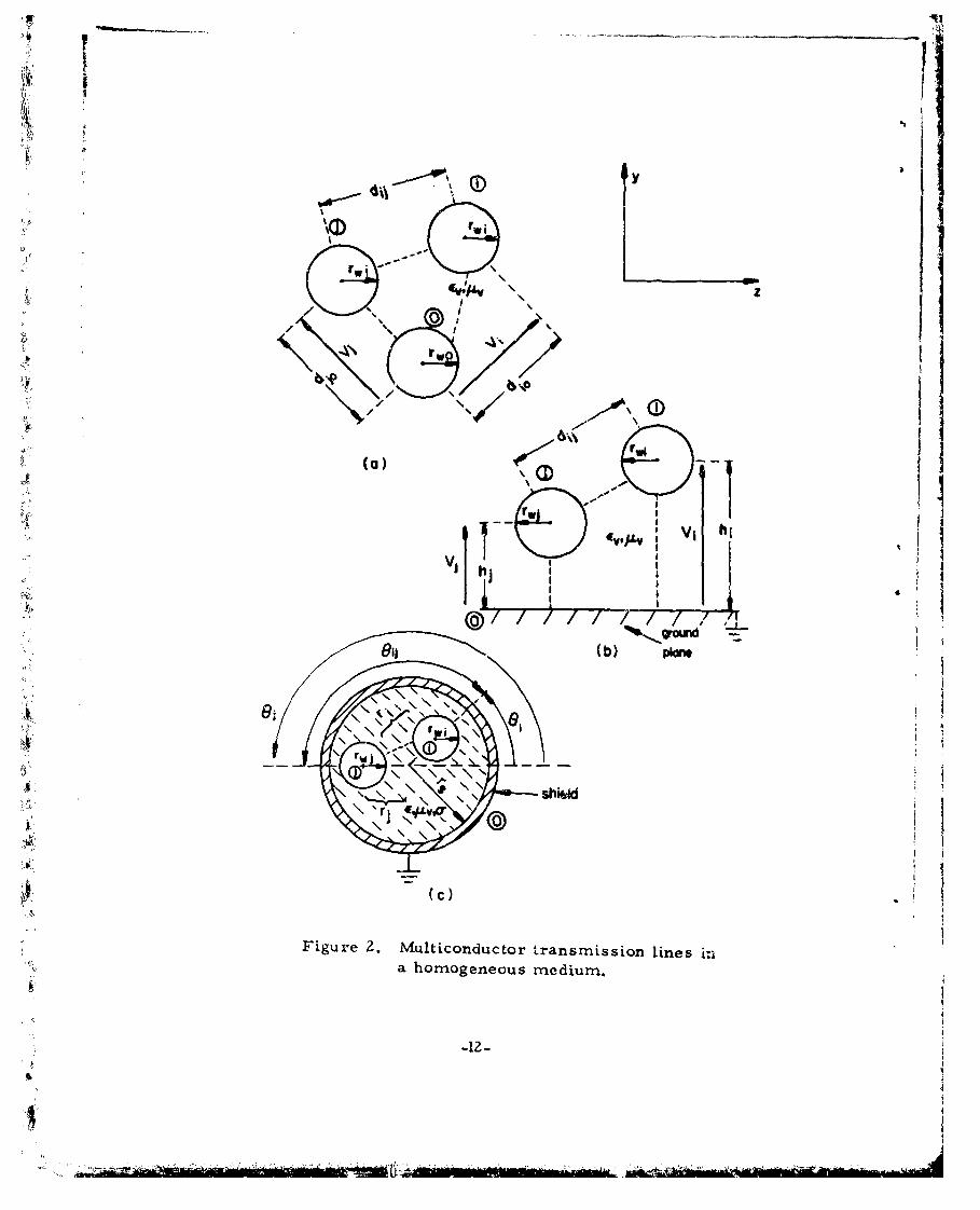
as cross-sectional views in the y, z plane in Fig. 2 and Fig. 3. In rig. 2,

n wires: (circular conductors) are shown with another conductor, the refer-

ence conductor, denoted as the zero-th conductor. In Fig. Za, the reference

conductor is also a wire whereas in Fig. 2b and Fig. 2c the reference con-

ductors are an infinite ground plane and an overall circular shield respec-

tively. These lines are uniform and the surrounding medium is hoinogen-

eous. In Fig. Za and Fig. 2b, the surrounding medium is free space with

parameters ev and uv. In Fig. 2c, the medium within the circular shield is

homogeneous with parameters e, uv and a. (The permeability of all dielec-

trics in this report will be considered to be that of free space, Uv.)

In Fig. 3, similar cases are shown with the wires having circular

dielectric insulations (an obviously very common situation). Thus the

medium in each of these cases is inhomogeneous although the lines are

nevertheless uniform. The permeabilities of the dielectric insulations are

considered to be that of free spa-ce, L± v, as is typical of diole':ff'ics. Each

dielectric insulation is described by the scalars permittivit., £,, ard con-

ductivity, ai, i=0, l, ---- ,n and the space surrounding the dielectr., "

tions is considered to be free epace.

The corresponding cases for the more familiar two-conductor lines-¢ t

(n=l) are shown in Fig. 4 and Fig. 5. Note in Fig. 4 that the lines of E and

4'H are shown perpendicular to each other. This is a natural consequence of

A-11-

S. . . . . ..... . .

pJ

i: Vi

I--

I'

MI

"\ ~

J[

• "••;'(a)-

I v h•2f _ _

I 4,

4'"

•.;

(c)

>> Figure 2. Multiconductor

transmission lines i,:i

c, ~ a homogeneous

medium.

L

- 12-

__ _ I

I'.' I'.

i/

I

0Ev,/.Lv

7 / / © b) ground

Figure 3. Multiconductor transmission lines in aninhomogeneous medium (cont.).

-13-

I

ii•I

Shield

© ~I

I(C)

iii

Figure 3. Multiconductor transmission lines in aninhornogeneous medium.

-14-

a~i

: ty

*, -, -r -WI:

rH

- FI

I IX=O X.

(a)

ly E.

, fX=.01

" 4 (b)

z Yground pae

(c)

z II

F:gure 4. Two-conductor transmission linesin a homogeneous mnediumn.

-15-

S.... ., ' "~i~ i:'a"i"shiel ...

4 ~

d IvII'v

I I

x=O (a) X=

h "ii•///// X, o0')®////,,/

ground plone 9

(b) .)) 9

, v

"" 0(c) Microstrip grudpae /

S ii

!''Figure 5. Two-conductor transmission lines

in an inhomogeneous medium (cont.).

-1I6- '"1

::. ;:•,.•._,;::• , i•i ' '• • :'•:J = -, •: . ,•i'•,; €:• -. -,,I.•••; .• :':l •• • :: = , •' • '-: ._: • • • " i -.•' .:: " '••;, • : ; •=',-:• :I I•,' ..' :,

- *rr 'w - . - re ' - - - -

Ir

r s

shield

Figure 5. Two-.concluctor tranarnjission linest irn an inhOrnogeneous niedium.

-17-

the TEM mode assumption [40].

If the medium is homogeneous as in Fig. 1 and Fig. 2 and all (n+l) con-

ductors are perfect conductcrs, then losses in the medium can be included

without violating the TEM mode assumption or the uniqueness of the voltage

and current definitions [40]. However, in the case of a homogeneous me-

dium in Fig. 2, it is only logical to consider a lossy medium for the case in

Fig. 2c since the surrounding medium in Fig. 2a and Fig. 2b is considered

to be free space. Dielectric losses can be introduced through a finite, non-

zero ohmic conductivity, a d' (which generally will be quite small for typi-

cal insulation materials) and also through dipole relaxation effects [30]. To ]

include both of these effects, we may consider the material to be charac-

terized by a complex, effective permittivity (which is frequency dependent)

instead of a real permittivity. To include dipole relaxation losses, the per-

mittivity may be considered to be complex as [30] e = d -je". Ampere's

law in a homogeneous medium possessing both of these loss quantities be-

4 -4 4C + W ll -1

comes VXH = ad E + jW CE = [(d + we") + jwe']E = jw ' [ 1-j (d+ve").

The real part of the complex permittivity is expressed as E' = ev Cr where

ev is the permittivity of free space and c r is the relative dielectric constant.

The effective conductivity of the ho ogeneous medium ther. becomes

a = ad + w ". Thus the losses of the medium may be accounted for by using

a complex effective permittivity ceff = e (l-j tan 6) instead of a real per-

mittivity and tan 6 = a/(w ev Cr) is the loss tangent of the material [40].

Ordinarily, the loss tangent and the relative dielectric constant Cr zrer8

given for materials as a function of freque,3cy. Therefre, it is quite clear

that for (n+l) perfect conductors in a homogeneous medium, losses in the

medium, i.e., q #0, can be included without violating the TEM mode

assumption or the uniqueness of the voltage and current defiDitions since the

real permittivity for the lossless case (c, =0) is merely replaced by a corn-moe ei f to account for losses in the medium.Se

tmode assumption is legitimate for the lossless, homogeneous case, there is

no reason why the use of a complex permittivity instead of a real permit-

tivity should change this.

The lumped-circuit model for a 6x length section of the two-conductor

lines in a homogeneous medium in Fig. 4 are shown in Fig. 6. The linesI

have a total length £ and Thevenin equivalents of the linear terminations at

the ends of the line are shown.

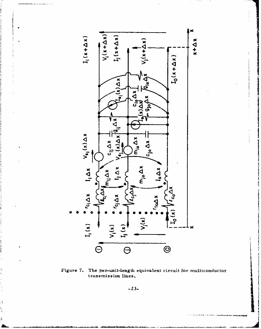
The lumped-circuit model describing the TEM mode of propagation for

a &x length section of any of the multiconductor lines in a homogeneous

medium in Fig. 1 and Fig. 2 is shown in Fig. 7. All & x length models for

other sections of the line will be identical since the line is uniform. Since

the cross-sectional dimensions of the line (conductor spacing, wire radius.

etc.) are all assumed to be "electrically small" and &x is assumed to be

"electrically short", then it is valid to characterize a &x section of the line

with a lumped equivalent circuit.

Resistance elements rc r ci r cj and conductance elements gi0s gj 0 ,

gij are included to represent losses associated with the conductors and

-19-

'4-

N • ,

"iu T" ts

(20) zo-

~~y-~-- •.

K I ''K 4

4

+ 31 +4PC 410

00

040

"-"o "o

-m 0_ 0

. 1C

L

I-I M

VT-op

Figure 6. The termnination-networksaneqilntcrusfotv' -cc.nductor transmission lines (cont.).

M$

- 21.

I V(

VO I() I t() , .

,•6v~o•- A',, tax

II~ i

(C) I

I a~l

(d)

Figure 6. The termination-networks and equivalent cir,-uits for

two-conductor transmission lines.

S~.22-

-1S

K Kx PC K

- '1%+

x PC

0 0

Figure 7. The per-unit-length equivalent circuit for multiconductor

transmission lines.

-23-

medium respectively. The inclusion of a surrounding medium having a

finite, nonzero conductivity and dipole relaxation losses with these sI,,nt

conductances is consistent with the assumption of TEM mode propagation

whereby no longitudinal conduction or dieplacement current can flow in the

dielectric and any current flow in the mediuri i.s confined to the transverse

plane. The shunt conductances account for the portio-as of the transverse

currents associated with conductive and dipole re)axation losses of the

medium, i.e., the transverse displacement and cor.ductic currents due to

the imaginary part of £eff* Similarly, shunt capacitances account for the

transverse displacement currents associated with the real part of eff.

Also self inductance terms for the conductors, lot Ai R.; mutual inductances

between the conductors, mn., r inm..; and mutual capacitances between theoi, 0

conductors, ci 0 , c , c.., are shown [ 3 9). Lcjsy conductors also produce a

portion of the self inductances due to skin effect which is represented by the

elements Ic0, , c which are internal self inductances produced by cur-Co c1 cj

rents internal to the lossy conductors [2, 3, 30]. The infinite ground plane

and circular shield in Fig. 2b and Fig. 2c are considered to be perfect

conductors and for these cases rc0 0 = 0. A method of including a lossy0

ground plane is given in [29] and is frequently used to represent the earth

return path in power systems [13].

Some care must be exercised in interpreting the elements g,' lip P

and m 0 , rn- 0 , mij as strictly "self inductances" and "mutual inductances"ioLi

respectively in the conventional sense. This interpretation relies on the

-24-I :

property that the surn of the currents (at a particular x) associated with all

n(n+l) conductors is zero, i.e., 'F I.(x) = 0. An excellent discussion of this

is presented in reference [3], Chapter 1 and the reader is referred to this

for further clarification. Our results will not rely on this interpretation

since we will not determine these individual external inductance parameters

but will instead obtain the per-unit-length external inductance matrix, L, of

the line directly. The entries in L, which are the essential items in our ,

analysis, will be linear combinations of these per-unit-length "inductances"

and once L is determined, there is no need to separate its entries.

All of the terms resulting from losses, rc0, r ci, rc, 0 gi 0, gijo ta€0

Lc are, in general, functions of frequency. The external parameters,

Io P0 P lip' mij* m0r ,. 0 , cij, ci0, cJ0, gi0, gj0. gij. are derived assuming

perfect conductors such that the transverse fields satisfy a static distribution

"k at each x along the line [39]. These external parameters will also be func-

tions of frequency if the permeability, permittivity or conductivity of the

surrounding medium is a function of frequency. In this case, the parameters

are recomputed for each frequency assuming the transverse fields satisfy a

static distribution at each x along the line. All parameters are per-unit-

length quantities and therefore the total value of each parameter for a &x

length model in Fig. 7 is the per-unit-length value multiplied by the section

length, 6 x.

It is important to note that this is an exact representation of the TEM

mode of propagation for (n+l) perfect conductors in a homogeneous medium

-. 5-

. ..... ........ . . ........ . ..... . . . . . . . . . .-..--- . .

1

as in Fig. 1 and Fig. 2. Imn-perfect conductors are considered as an approxi-

mation throughr0, rc, rc "O / £ under th,. issumption that thematio0 thog rcri Ci, O 0 J'il1

conductivities of the conductors are very large and much greater that the

conductivity of the dielectric medium so that the fields structure is essen-

tially TEM. Although the presence of an inhomogeneous medium as in Fig.

3 precludes the existence of the TEM mode except perhaps in the limiting

case of zero frequency, the equivalent-circuit representation in Fig. 7 will

be assumed to be an adequate representation for the quasi-TEM mode for the

lines in an inhomogeneous medium in Fig. 3. The parameters for thit case

will also be computed at each frequency by assuming (as a first-order

approximation) that the field vectors are entirely transverse and satisfy a

static distribution at each x along the line.

For the two-conductor cases in Fig. 4, the transmission line equations

can be derived from the A x equivalent circuits in Fig. 6 for the sinusoidal,

steady state in the limit as Ax -+ 0 as a pair of coupled, first-order, ordi-

nary, complex differential equations [2, 3]

d V(x)[ x + (r +jWAt +jwt,) I(X)=0 (la)

+ (g + jw1c) V(x) =0 (lb)dxY

where Z and Y are the per-unit-length impedances and admittances of the

line respectively. For each of these cases, rc rcl rc0, + 1,Cl Jc0,

= L1 + £ 2l0c c10 and g = gl 0 . If an incident electromagnetic field

illuminates the line of Fig. 4a, the equations in (1) are modified to include

the effects of the incident field and become [20]

-26-

d V(x)4 Z~'. I V (x) Ve , "---dx 8 ~ )=V ()(a

d I(x)+ Y V(x) I W) (2b)

where Vs(x) and Is(x) are distributed sources along the line induced by the

spectral components of the incident field and are given by [ZO]

•d (inc)

Vx) = jwu Hz(yx)dy (3a)0

•:: d (inc)

3 Is(X) = -Y E (y,x)dy (3b)0

The two wires in Fig. 4a lie in the x, y plane with wire 0 at y = 0 and wire I

at y = d. The components of the incident magnetic and electric field intensi-

A (inc)ties at the radian frequency W in the z and y directions are denoted by HZ(y,'

(inc)and.y, x), respectively.

Similarly for multiconductor lines, the transmission line equations can

be derived from the equivalent circuit in Fig. 7 for the sinusoidal, steady

state in the limit as Ax -+ 0 as a pair ol n coupled, first-order, ordinary,

complex differential equations in matrix form as (see Appendix B)

(x) + Z(x) vs(x) (4a)

i(x) + Y V(x) =I (x) (4b)

which may be written in an alternate form as a set of 2n coupled equations

in partitioned form as

V(x) V(x) [V 1X+ 00

S0 (x) x)

-27-

'7lii

A matrix, M,, with m rows and n columns is said to be m y n and the ele-

ment in the i-th row and j-th colur.'a is designaated [MI.. with i=l,---, m

and j=l, --- n. The dot (o) denotes first derivative with respect to x, i.e.,

d_[r(x)]i = -•- V (x), and 0 is the mn ) n zero matrix with zeros in every

position, i.e., [ O0 ij = 0 for il, --- , rn and j=l, --- ,n. The elements of

the n 'X 1 complex column vectors V(x), I(x), Vs(x), _Is(x) are [V(x)]i = Vi(x),

if(x)]i = I i(x), [V~s(x)]i = Vs (x), [Is(X)], = Is i(x) where the element of an n -X 1

column vector V with n rows in the i-th row is denoted by [V]I for i-l, --- , n.

The per-unit-length series voltage sources, V. (x), and shunt current

sources, Isi(x), are induced by the spectral components of the incident

field and are complex-valued and functions of frequency and position, x,

along the line. For (n+l) wires in a homogeneous medium in Fig. 2a, these 4sources are shown in Appendix C and in [27) to be

d 0 (inc)(x) = Hni (ti. x) dti (5a)

0

{ n .•ioE

Isi~x) = W (gi0 + jwV c.0) + SZ (gij + jE i ) .x) di (5b)j~l0

n f gj+jWcj djo (inc)+t F , E x ) d

where ti is a straight-line contour between wire 0 and wire i and perpendic-ular to wire 0 and wire i. i (tx) and Einc)

(o)ni (ti (ix) are the components of

the incident field vectors normal to a plane formed by thi. two wires and

-28-

parallel to g (transverse field) respectively. Solutions for V8 (x) and [a(x)1 1

for 'he other configurations are discussed in [22, 24, 251 and Appendix C.

The n n complex-valued matrices Z and Y are the per-unit-length

impedance and admittance matrices respectively and are symmetric, i. e.,

Z = Zt and Y = Y where the transpose of an n n matrix Mis denoted as

Mt. These matrices are independent of x since the lines are uniform and

are separable as

Z =R +,j•L +jUL (6a)

Y=G + j C (6b)

where R and L are the per-unit-length conductor resistanct and conductor

internal inductance matrices respectively and are real, symmetric. The

external parameter matrices, G, L and C, are real and can also be shown

to bt symmetric (for linear, isotropic media) regardless of whether the

medium is homogeneous or inhomogeneous thus permitting the equivalent

circuit representation in Fig. 7. [39]. The matrices G, L and C are the

per--unit-length external conductance, inductance and capacitance matrices

respectively. The entries in these matrices are obtained in Appendix B

and are given by

[4[R 1,j r (7a)

0

i~j[L + [L I..= n..r.-n (7b)

IJ 0 1 0i~j

[L]ii=£ + O am0 [L]L =j A0 + m.~j mi0- m0 (7 c)

14j

_29-

n[G = + E 9 [G.ij = -g.. (7d)

j 1Ji~j i~j

ntn

[C C co + F c.. [I[] - c.. (7e)j=l

i Vj i#j

for ij = 1, --- ,n. C and G are said to be hyperdominant since each term on

the main diagonal is greatei than the sum of the elements in that row [39]

and they can therefore be shown to be positive definite meanini: that a)l n

eigenvalues of C and all n eigenvalues of G are positive and nonzero [41].

4 The derivation of the :)er-.unit-length parameters will be discussed in Section

,•V,

-30-.

.I

Ill. SOLUTION OF THE TRANSNIlSSION LINE EQUATIONS

The set of 2n first-order, complex-valued, ordinary differential equa-

tions in (4c) which describe the transmission line for the TEM mode of pro-

pagation and the sinusoidal, steady state are in the form of state variable

equations [38,42]. Systems of first-order differential equations in the state

variable form have received considerable attention in recent years in the

general area of linear systems and the solution to (4c) is

V~)Y(xo) A (x

[x) (X,x [i( 0 + ,(x, ) di (8)T' x0x.

where O(x,x 0 ) is the 2n X Zn comple.c-valued state transition matrix which is

the solution to (4c) withVs(x) = Is(x) = n1 and the parameter x 0 is some

arbitrary fixed point along the line [38, 42]. .

Obviously the difficult portion of the analysis (aside from the difficulty

in computing the per-unit-length parameters and equivalent field excitation

"sources in V (x) and I (x)) is the determination of the state transition-s

matrix or chain parameter matrix, .(xx 0 )" Fortunately, for uniform lines

where Z and Y are not functions of x, the solution is fairly simple as will be

shown (although there are some important computational problems when

losses are included). For nonuniform lines where Z and Y are functions of

x, i.e., Z(x) and Y(x), (4c) becomes a set of nonconstant-coefficient differen-

tial equations (Bessel's eqaation is an exa.nple of a nonconstant-coefficient

differential equation) [43-46]. For these types of lines, (8) holds but the

ultimate difficulty is the determination of the state transition matrix and

-31-

- -

except for some very special structures one must resort to numerical

methods and approximations to obtain 0(x,xO) [42]. If the line is "abruptly

nonuniform" as with branched cables, i.e., consists of uniform subsections

in cascade, then the overall chain parameter matrix, I (xo), is the pro-

duct (in the appropriate order) of the chain matrices of the individual

uniform subsections between x and x0 and thus is straightforward to obtain.

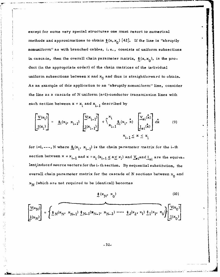
As an example of this application to an "abruptly nonuniform" line, consider

the line as a cascade of N uniform (n+l)-conductor transmission lines with

each section between x x. and x. described by

r [A

V(xj) V(x._ li A Z .(x) A: L1'+ xiil) + (xi, x) dx (9)

I~~Xxl I (X xi X.s i

for i=l,---, N where §i(xi x. is the chain parameter matrix for the i-th

section between x xi and x =xi (xi_1.c x< xj) andVliand Is are the equiva-

lentlinduced source vectors for the i- th section. By sequential substitution, the

overall chain parameter matrix for the cascade of N sections between x and0

xN (which are not required to be identical) becomes

i(xN, x0) (10)

YvxNil Y [(xoi

=) [N(XN" XN.I) N.I(xN-l' xN.2) ..... I 2 (x 2 , xV) • 1 (xl, x0

II I-32-

iI

V!

N-1 6 A

V I.

0(AA

}i " N(~'4 * xN. , ,XN.) •N SlXN~, XN.) *.. .. •~ (X ..l, x.) C •(i,•

is+x. (

!;(•xN 3~ N x] A

XN I

The overall chain parameter matrix for this cascade of nonidentical line

sections between x = x0 and x = xN is identified in (10) as the matrix product

V(xN, x0 ). Note that the indicated order of multiplication of the individual

chain parameter matrices must be preserved since they do not generally

commute. Lumped-element networks at discrete points along the line can

"also be incorporated into the problem by writing the n2atrix chain pararne-

ters of these networks and including them appropriately into the product of

the chain parameter matrices of the individual uniform sections in the above

manner,When the line is uniform (as is being considered here) where Z and Y

are independent of x, the state transition matrix, t(x,x 0 ), can be shown to

be a function of only one variable; the difference quantity (x-x0 ) r421. Thus

for uniform lines, we may denote the state transition or chain parameter

matrix as O(x- x0 ). The state transition matrix has the property that

S(xO, xO) 1In where 'Zn is the Zn y 2n identity matrix with [,2n'ii l and

[12nij 0 for i,j = 1, --- , 2n and i~j [38]. This should be clear from (8) by

setting x equal to x0 . Additionally, it may be shown that •-(x,x 0 ) =(x 0 , x)

where the inverse of an n n matrix M is denoted by M and therefore the

"-33-

inverse of the chain parameter matrix may be trivially determined [42].

This is quite obvious from (8) for VX(x) = I (x) = 0 by interchanging the

roles of x and zoo

For two-conductor lines (n=1) the transmission line equations become a

set of two complex-valued, ordinary differential equations given in (1). The

solution of the transmission line equations for two-conductor lines can be

obtained quite easily by differentiating (lb) with respect to x and substituting

(la) to yielddl I(x)dx2 Y Z I(X) (I

= V2 I(x)

where the propagation constant, v, is

TY Z (12)

The solution to (11) becomes

M(x) = eVx I+ - eVx T" (13)

where I+ and I- are complex, undetermined constants. Substituting (13) into

(lb) yields

v(X) in tesli I+ + I z ; ;1: (14)

where the characteristic impedance, ZC, is given by (

F." =Z/Y =/Z . (15) I

To find the solutions in the time domain, multiply (13) and (14) by ej t to"

obtain l., (j11t + Vx) "!••.• '(,t) Z [ C e 0jtot - y-X) I+] + Z C e -](16a)

S "•'+xt (, t)

-34-

4'

i J ~(x,t 0 le 0jjt -x) +].[o ,,t + Yx) -](16b)

Therefore the total solution consists of waves traveling in the +x direction

!(forward-traveling waves) denoted b•y 7/(x, t) and j +(x, t.) and waves traveling

in the -x direction (backward-traveling wavez) denoted byif(x, t) and J(x, t).

SThe characteristic impedance, ZC, is the rati', of the voltage and current in

the respective waves.

k For two-conductor lines, the chain par, ..ýter imatrix is Z -X 2 and can

easily be shown to be [2, 3]

~(xx~)= osh tv(x-xO)} -ZC sinh fy(x-xo{'(x xO)(17)

[~~sinhfllV(x-xoq cosh {Y(x-x0 )lJ

where cosh and sinh are the hyperbolic cosine and sine respectivey.

Note that the determinant of the chain parameter matrix is unity. Knowing

this quantity, the solution for the voltage and current at any point, x, along

the line can be found from (8) in terms of the voltage and current at some

reference point, x0 , as

V(x) = cosh fY(x-xO) IV(xo)- ZC sinhf1v(x-xO)]l(x0j) (18a)

+ cs x*)V 8(x') - Z C sinhvXA)J I s(X)] d

1W - sinh y(xxO) V(x) + cosh fy(x-,x I(x-x) (18b)z-c

-Z B inh [Y(x-X')' V5 (X') + cosh fY(x- X)j .~(A), d.ýc CJ

-35-

I*

For multiconductor lines, the equations in (4c) may be thought of as

"strongly-coupled" state variable equations since the bluck off-diagonal

terms, Z and Y, are nonzero whereas the block main-diagonal terms are

zero, 0 . The chain parameter matrix, I(xx 0 ), however, may be dater-n-n

mined in the following manner which is similar to the method for solving the

two-conductor line employed above [18, 26, 471. Assuming for the moment

that Vs(x) =1 (x) = n 2 1, differentiating the second set of equations (4b) again

with respect to x, I(x) = -Y V(x), and substituting the first set (4a), Mx) =

-ZI(x), one obtains the set of n second-order differential equations

Irix) = Y ZI(x) .(19)

Note that even though Y and Z are symmetric, it is not necessarily true

that the matrix product Y Z (or Z Y) will be symmetric.

The solution of (19) is usually obtained with similarity transformations

[13, 18, 26, 38, 41,42,47, 48], which is referred to in the power transmission

literature as "modal decomposition" [13]. Define a change of variables,

I(x) = TIm(x) where T is an n-Xn nonsingular, complex-valued matrix and

_I-(x) is an nXl complex-valued vector of "mode currents". Substituting

this change of variables into (19) yields

I .T.YZT1 (20)

Suppose there exists an nyn similarity transformation, T, which dia-

gonalizes Y Z, i.e.,

T-1 YZT (21)

where y 2 is an nxn diagonal ni-%trix with

-36-

Ii

•]i= ",i(•ZZa)

(22b)

and the terms, y•, i 1, --- ,n are complex-valued scalars. Then (20)becomes a set of n uncoupled differential equations with the simple solution

(18.26.47]

!(x) = TIm(x) (Ž3)

T eYX + YX-

where ý is an n)(n, diagonal rmtrix with Y!ei x (24a)

0j (24b)nd + I•andI and U are nyl vectors of 2 n complex, undetermined constants,

1± -[1 +1i and I*: = [,I ]iw which will, in general, be functions of frequency[47). These undecern-ined constants will be evaluated by considering the

boundary conditions or terzination-networks at the ends of the line. Sincefrom (4b) fix) - Y V�x), one may obtain from (23)

. y x (x)x) x (25)clx

-(e + ex

-37-

_ _ _ _ _ _

where y is an nxn diagonal complex-valued matrix with

[]. - -. (26a)

[y.. =0 (26b)

i~j

One can easily show from (21) the identity y 1 Ty = ZT y 1 which is used in

(25).

The solution ir, the time domain can be found since V(x, t) = V(x)eJ t

and J(x, t) =I(x)eJI1~t by multiplying (23) and (25) by et. It should then be

clear that the total solutions consist of forward-traveling waves, t+(x, t)

J +(x, t), and backward-traveling waves, 3" (x, t), 2 (x, t), on the line with

[18]

_+X_.(x, t) L/ y(x, t) + ""(x, t) (2 7a)

J_(x, t) = J•(x, t) - .- (x, t) (27b)

where -tJ_(x, t) = T e"Ix I + ejWt (2 8a)

J-(x,t) = T e'x I e jWt (28b)

4--

N.%,, t) = Zc _ t) (28c)

7e"- (x, t) = Zc C; (x, t) (2 8d)

and ZC is the "characteristic-impedance matrix" relating the voltages and

currents in the waves with Zc defined from (23), (25) and (28) as

SZ=Y-1 T T-1 =Z T Y- T-1 (Z29a)

z ~y Z(F V *r (2 9b)

-38-

v'I

The symbolic notation in (29b) conforms to the scalar characteristic imped-

ance for two-conductor lines discussed above. It can be shown that [18]

T Y T-1 (30a)

7Z27 Y/i Y (30b)

-Y/Z. Y 1 (30c)

The relations in (30) may be easily shown [18] by forming =Z) ) =

•Z,-,Y. Note thatz i y and the order of multiplication of the matrices

cannot be interchanged si.nce Z and Y do not~in general, commute.

If the mode currents, I.(x), are defined as in (23) and the mode vol-

tages are defined from (25) as V(x) = Z; TVM(x), then it is clear that the

mode quantities consist of n uncoupled waves and each mode has the propa-1 ' gation constant Yi. The velocities, vi, and attenuation constants, •i asso-

ciated with each mode are found by writing Yi = ni + j(w/vi) where ni and vi

are real scalars. Thus one might think of these "mode" quantities as beingIIso1Llewhat basic quantities in the overall propagation of the waves since the

total voltages and currents are linear combinations of the mode voltages and

mode currents rospectively. This concept, however, is not particularly

useful in obtaining numerical solutions to a given problem via machine corn..

putation and is only offered as a link to the more familiar two-conductor

case discussd above. There are, however, instances where this concept,

when related to matrix scattering parameters, can prove useful in certain

synthesis problems [19].

_39-

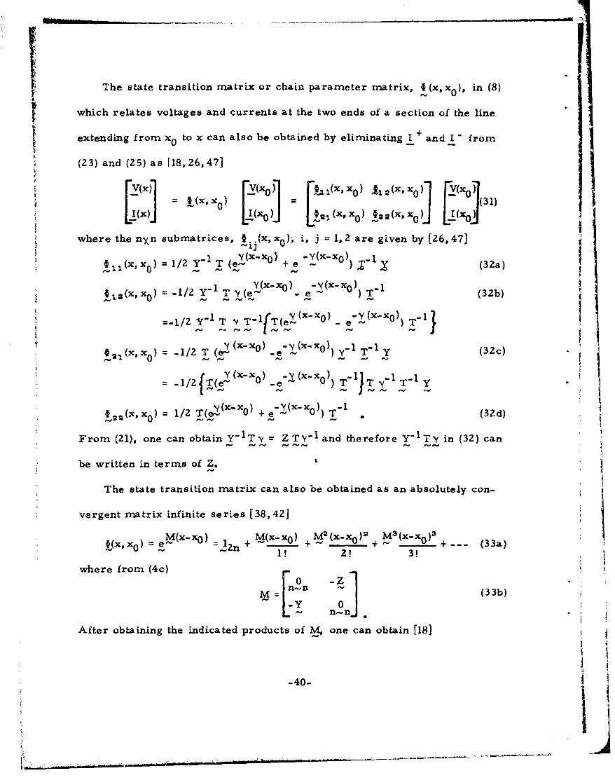
The state transition matrix or chain parameter matrix, 0(x, x0 ), in (8)

which relates voltages and currents at the two ends of a section of the line

extending from x 0 to x can also be obtained by eliminating I + and I - from

(23) and (25) as [18, 26, 47)

X XOj1A - I(X(, xO) 2aa(XiO xO0 (31)I(X L!X :2(IO L L- IX21

where the nxn submatrices, • .(x,x 0 ), i, j = 1, 2 are given by [26, 47]) ~ij

(x, X 1/2N Y-1T (eX-X) -1~e ,T" Y (32a)

X 1 xx) -12Y1 (-o) -Y(x Oo 1/2 (e - e (32b)

ig<xx")e-llx-Y0) -

1=-/2 Y-T1ý T y(xx 0 ) - e T"I

-Y .e-O -Y (X- Xo)) Y09=(x,x -1/2 T -(e-. ., T, 1 Y (32c)

- o/ T -e "

{ l/ (X'Xo)_e- •0 X-XO))

x = 1/2 T(eY(xx) +e(x(x0))T 1 d)

From (21), one can obtain Y-ITY ZTY 1 and therefore Y- 1 Ty in (32) can

be written in terms of Z.

The state transition matrix can also be obtained as an absolutely con-

vergent matrix infinite series [38,42]

( eM(x-x) = + M(xxo) +M 2 (x-xo) 2 M 3 (x-x 0 )3

Xx)-e~ 1z+ + + + (33a)"" 1! 2! 3!

where from (4c)

M =(33b)

n-,nj

After obtaining the indicated products of one can obtain [18] 3

-40-

i.U- .i- ~ -- -

+XX) (x-xo)4

(xxO) I n z Y+ + (,17 (345!

Y_~ ~ + Z+ , Za

(xXrP (x-x0 )5!12xsx -Z(iXO) Z Y XO y+ ( ZY)

+ 3 ~ ~ ) (34b))

=(_o +F IT(x- ) 3T!

+ 5(~5

(XXo) + ZX3(4!

+ )-t5 XX Y-1

-411

(XX (x x Z ( -X )3 (Y )2 Y (4c

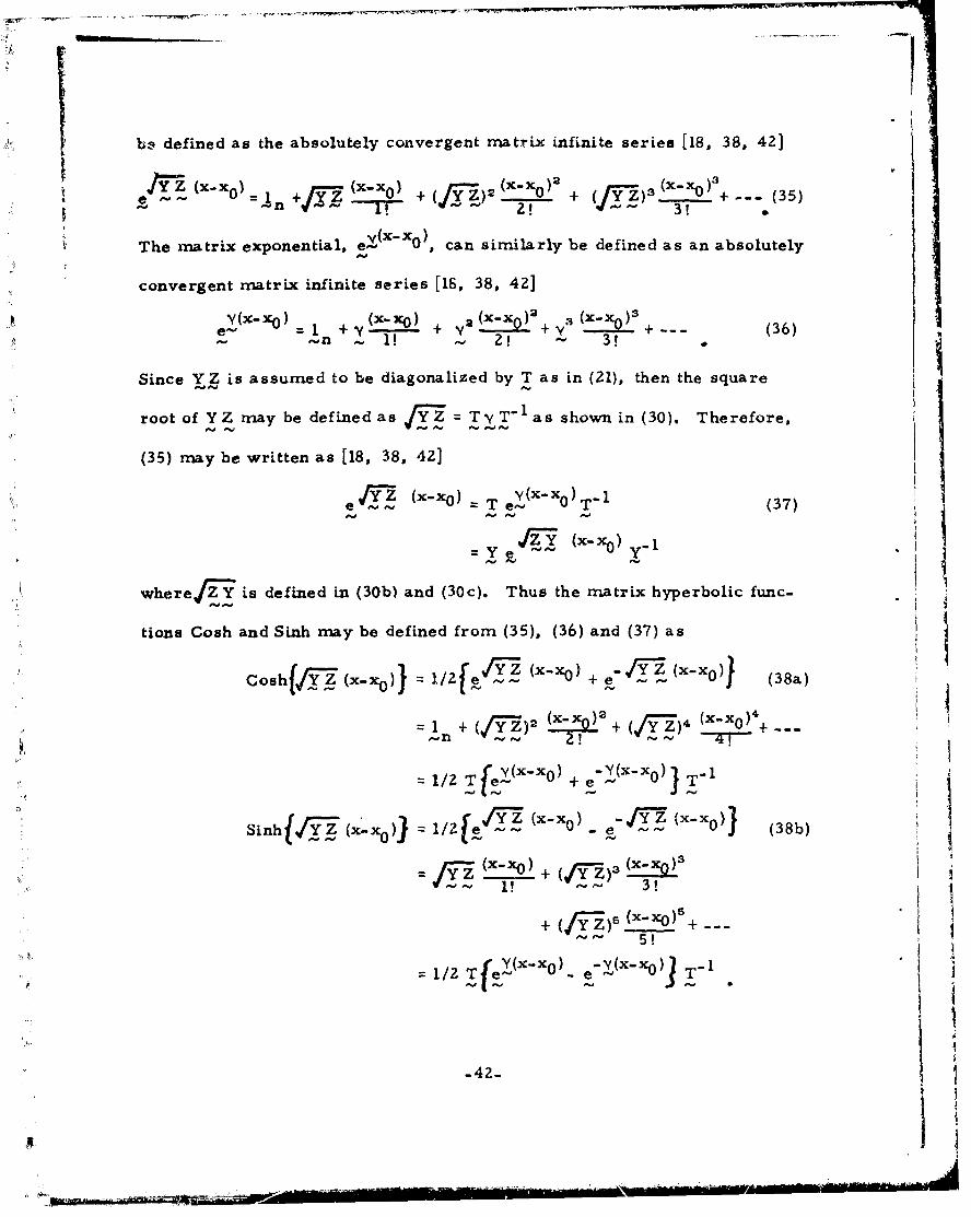
qbe defined as the absolutely convergent rmatdrix infinite series [18, 38, 42]

S(X-Xo) + ((/7) )2x (XX (X-xo) (35)

SThe matrix exponential, eX(xxO), can similarly be defined as an absolutely

convergent matrix infinite series [16, 38, 42]

Y(X-x 0 ) (x-xNO) 2 (xxo)2+ Y 3(

)= + ' ' + -+- (36)-n 1 2! 3! 3,

Since YZ is assumed to be diagonalized by T as in (21), then the square

root of YZ may be defined as T= T -T as shown in (30). Therefore,

(35) may be written as [18, 38, 42]

-' (x- )-Ye (x-x 1

where/ZY is defined in (30b) and (30c). Thus the matrix hyperbolic func-

tions Cosh and Sinh may be defined from (35), (36) and (37) as

e/i71-Y (x-xo)J (8a

Coshf/ (x-XO)J i./Zf ev Y Z 0x + e3a

= + ( 2•,/7z - X. ()T+ z), (xxo)4

~n -. , +2!T ( 2 !-Y(x-xo-

1/2 T +e T-1

Sinh( ý/7Z~ (x.'xo)J = /2?e - (x-x0) - ly Z (x'Xo) (38b)

r (x-xo)+(/'Z)(

+ (y-Z)3 (x-xo)+.

5!

1=I/2 TeY(x-x0)- eYT(xx01)TT"

-42-

Therefore, it should be clear by utilizing the relations in (35), (36), (37)

and (38) that the expressions for the chain parameter submatrices In (32) and

(34) are equivalent and may be written symbolically as [18]

§11(~xo =Goshf,/T71 (x-xo)l Y-1 Gosh f1/77Z (x~xO)I Y (39za)

0 yyZ) 1Sinh{/?(x- xO) SihV7 (x-xo)J VT:T

021 (X, Zc Sinh/~ (xx)TY = (-SinhSih //T : (x x0 )} ~ z VZ)'

S~(39c)Z z-1C S(/ ['/E Si Xf/Z (x~x 0 -Sinh{1 (39c)Xxo

Cosh f T(x-xo)} X Gosh f/ X7 xOx)} Y_ 09d)

where the characteristic-impedance matrix, Z., its defined in (29) and (30).

(Note that these reduce to the scalar elements for two-conductor (n=l) lines

in (17).) For numerical machine computation, however, one would use the

forms of the submatrices given in (32) since the equivalent expressions in

(34) and (39) would be of little practical value in obtaining numerical results.

Also one can show certain fundamental matrix identities involving the

subrnatrices of wne chain parameter matrix [18]:

Identity 1: t' = A92 =In (40a)

Identity 2: 2 1 2 9 1 4n, ~1

Identity 3: ý12 2 012 = (40c)

Identity 4: (40d)

tIdentity 5: Oil = 22 (4 0e)

-43-

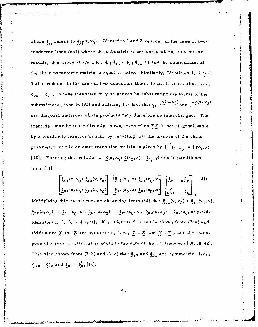
where L • refers to ýij(x, x0). Identities I and 2 reduce, in the case of two-SAl, ,j

conductor lines (n=1) where *-,e. submatrices become scalars, to familiar

results, described above i.e., 4, a III- =2 09, = land the determinant of

the chain parameter matrix is equal to unity. Similarly, Identities 3, 4 and

5 also reduce, in the case of two-conductor lines, to familiar results, i.e.,

= t These identities may be proven by substituting the forms of the

Y (x-x 0 ) -Y(x-x 0 )submatrices given in (32) and utilizing the fact that y, e-'- and e

are diagonal matrices whose products may therefore be interchanged. The

identities may be more directly shown, even when Y Z is not diagonalizable

by a similarity transformation, by recalling that the inverse of the chain

parameter matrix or state transition matrix is given by 1-1(x, x0 ) =(xX)

[42]. Forming this relation as ý(x, x0 ) !(x 0 ,x) 1 Znyields in partitioned0 &Z

form [18]

[.l(xxO) x i 2 (xx0 •,i(XoX) 2(XO nX)°1 0 (41)

L~(X, X I 2 &xj L21(XO'X) §22(XOPxjo Xj 021 0 _ 2''- - -noJMultiplying thit result out and observing from (34) that (.(xx0 ) = (x' x),

•(ý -. (x 0 ,x), X 20(x,x 0 ) = - 2 (x0 ,x), I 2 (x,x 0 ) - I2(x 0 ,x) yields

Identities 1, 2, 3, 4 directly [18]. Identity 5 is easily shown from (34a) and

(34d) since Y and Z are symmetric, i.e.,, Z = Zt and Y ytP and the trans-

pose of a sum of matrices is equal to the sum of their transposes [18, 38, 42].

This also shows from (34b) and (34c) that 1 and 21 are symmetric, i.e.,

t t= 2and § 1-.1 [18].

-44-

"j

Thus the result conforms (symbolically) to the two-conductor case in

which Y and Z are complex scalars instead of matrices. This use of sym-

bolic notation for the square root of a matrix and the matrix hyperbolic func-

tions Cosh and Sinh of course makes sense because it was assumed that the

matrix product Y Z was diagonalizable by the similarity transformation, T.

It is not necessarily true that the matrix product Y Z (and also Z Y) will be

diagonalizable by a similarity transformation [41, 42•]. If the product is not

diagonalizable, then a sirmilarity transformation may be found to place Y Z in

the Jordan Canonical form and this result is found in [47] although numerical

results become more complicated to obtain.

Thus one of the important simplifying assumptions is that YZ is diago-

nalizable by a similarity transformation as in (21). It is often assumed that

YZ can be diagonalized by a similarity transformation regardless of the

numerical entries in Y and Z and this ispof course,not necessarily true

[41, 42]. To more completely investigate the problem, determine the eigen-

values of Y Z as roots of the n-th order complex polynomial in ve [18, 41, 42]

det yZ 0(42)

where det denotes the determinant. If the resulting eigenvalues, Y?, are

distinct, then diagonalization of Y Z is assured and the n x 1 columns of T =

[T _' , --- , Tn], Ti, are eigenvectors of YZ sati fyingQ T= 01?1 n-l 1 (43)i n rr-i

for i = 1, .. , n r18, 41, 4Z]. But.,ef course~one does not generally know a'

priori if the eigenvalues will be distinct and considerable computation may

-45-

~.

be required to determine this. If there exist repeated eigenvalues, then it

may or may not be possible to determine n linearly independent eigenvectors

via (43). If n linearly independent eigenvectors can be found, then diagona-

lization is assured [18, 41, 42]. It can be shown that the eigenvalues of Y Z - ~ iare the same as the eigenvalues of Z Y (see [42], pp. 101-102). When either

Y or Z are nonsingular, this can be easily shown by forming [18]

det (y2 1n -yZ det 2 1n - y-1) det f 2

det n -ZY since the determinant of a product of square matrices is ]equal to the product of their determinants and det (Y) det _Yl

det (Z') det (Z) = 1. Also one can form (43) as Y(y? 1 Z Y)•] T)

and Z-1 (y2 I _Z Y)(ZT.) T n201 so that if Y is nonsingular then each of

the eigenvectors of Z Y is equal to the product of Y-1 and each of the eigen-

vectors oi YZ (within a scalar constant), and if Z is nonsingular, then each

of the eigenvectors of ZY is equal to the product of Z and each of the eigen-

vectors of Y Z (within a scalar constant) 18]. These facts can be used to

form the relations in (23),(25) and (32) in terms of JýTand its eigenvectors.

When discussing the question of distinct eigenvalues in numerical com-

putation, it is important to consider the question of "how distinct". For

example, if two of the eigenvalues are distinct only after the 16-th digit,

then although they are technically distinct, the two eigenvectors from (43)

associated with these two "almost-distinct" eigenvalues may be very nearly

collinear causing T to be an ill-conditioned matrix with a very small deter-

minant, i.e., T will be "almost singular". Thus numerical instabilities

-46-

L .... . - • i ' • : ~ - . . • .• . :. . .!. . .. • =_ __ = ,•,,' --• i, _: • _'• .. . .

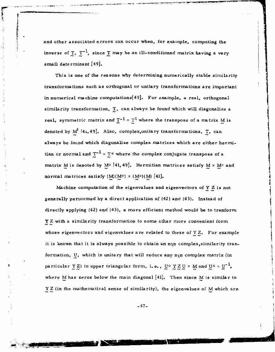
-• . -- ,,, , ,, .. .. .V.M"and other associated errors can occur when, for example, computing the

inverse of T, T-1, since T may be an ill-conditioned matrix having a very

small determinant [49].

This is one of the reasons why determining numerically stable similarity

transformations such as orthogonal or unitary transformations are important

in numerical machine computations[49]. For example, a real, orthogonal

similarity transformation, T, can always be found which will diagonalize a

real, symmetric matrix and T-1 = Tt where the transpose of a natrix M is

denoted by Mt f4L,49]. Also, complexunitary transformations, T, can

always be found which diagonalize complex matrices which are either hermi-

tian or normal and T-1 = T* where the complex conjugate transpose of a

o9 matrix M is denoted by M" [41, 49]. Hermitian matrices satisfy M = M- and

normal matrices satisfy (M)(M*) = (M':)(M)L4 [41].

Machine computation of the eigenvalues and eigenvectors of Y Z is not

generally periormed by a direct application of (42) and (43). Instead of

directly applying (42) and (43), a more efficient method would be to tranform

Y Z with a similarity transformation to some other more convenient form

whose eigenvectors and eigenvalues are related to these of Y Z. For example

it is known that it is always possible to obtain an n)(n complexsimilarity tran-

formation, U, which is unitary that will reduce any nxn complex matrix (in

particular YZ) to upper triangular form, i.e., U:-" YZU = Mand U: = U-

where M has zeros below the main diagonal [41]. Then since M is similar to

Y Z (in the mathematical sense of similarity), the eigenvalues of M which are

-47-

1'

the elements on the main diagonal of Mare the same as the eigenvalues of

Y Z r41,49]. A commonly-used algorithm ii the QR transformation [49]. The

eigenvecto-s of Y Z, T., are related to the eigenvectors of M, S., byT. =

US. where S. is in nxl eigenvector of M associated with the eigenvalue .y! and

corresponds to the eigenvector Ti associated with eigenvalue y? [41,49]. The

transformation to Hessenberg form is also commonly employed [49].

In addition to the question of the existence of a numerically stable simi-

larity trant-formation which diagonalizes the matrix product Y Z, there is

the problem of recomputing the eigenvalues and eigenvectors at each fre-

quency being considered. Since the matrix product Y Z is a function of

frequency, then one is, in general, required to repeat the determination of

the eigenvalues and eigenvectors of this complex-valued matrix product,

Y Z, at each frequency and this can be a very time-consuming task when the

response at a large number of frequencies is desired. There are, however,

certain practical cases where Y Z can be diagonalized by a numerically

stable transforrmaition and, moreover, for these cases, T is independent of

frequency and need only be computecd once. These important cases will now

be discussed.

3.1 Transmission Lines in a Homogeneous Medium

This section will consider the (n+l)-conductor lines in a homogeneous

medium represented in Fig. 2. Although the lines in Fig. 2a and Fig. 2b

can only logically be considered immersed in free space which is considered

lossless, the formulation which will be investigated will assume losses in

-48-

the medium in order that the situation in Fig. Zc may be considered. The

following important relations which are well known in the case of two-con-

ductor lines in a homogeneous medium are shown in Appendix A for the

case of (n+l)-conductor lines in a homogeneous medium which is assumed to

be characterized by U, C, a:

L C = C L = We (44a)

L G = G L = laI (44b)

When the dielectric medium is lossy as in Fig. Zc, the conductivity in (44b)

refers to the effective conductivity as a = ad + (1)" =W Cv Cr tan 6 and includes

the combined losses due to ohmic conductivity, ad, and dipole relaxation

effects. The loss tangent of the medium is denoted by tan 8, cv is the per-

mittivity of free space and er is the relative dielectric constant. The per-

mittivity, e, refers to the real part of the complex effective permittivity,

i. e., e = ev C r' and the permeability, ", will typically be that of free space,

~v. In addition, since the medium is homogeneous it can aI-o be shown [54]

that C = c K and from (44) it follows that

C = eK (45a)

L = "K- 1 (45b)

G = aK (45c-l

where K is an nXn real, symmetric, positive definite matrix independent of

e(and therefore frequency) and is dependent only upon the cross-sectional

structure of the line (conductor separations and wire radii). The matrix

product Y Z with the relations in (44) and (45) becomes

-49- S~I

YZ (a+ jwe) K (Rc + jt) L) + (jhua- W, U)O 1 (46)

aa.d if perfect conductori. are assumed, then all n mode velocities and

attenuation constants degenerate into one set, which represents the true

TEM mode of propagation.

If perfect conductors are assumed, i.e., R = L 0 , then from (46)"-c c n, n

T n and V? = (j~ti Uar- W2 uc) in (?,) where In is the n'yn identity matrix

with ones on the main diagonal and zeros elsewhere. Thus, the matrix

chain parameters for the homogeneous-medium case with (n+l) perfect con-

ductors become from (32)

§-= x 0 cosh y {(X- Xo0 )}In (47a)

=1 -x sinh {v(x-x0 )} [Wt/y) L) (47b)

- sinh {V(X-Xo)}[(jw-Iy)L]• 1 (47c)

§2XX0 cos (-X Ii (47d)

where v=Ijwu (+ jje) and the characteristic impedance matrix becomes

from (29a) G(

ZC =17-(, j)U K- 1(48)

- (jw/v) L

For a lossless medium, a = 0, y = jWmand (47) becomes [26]

=Cos $(X-XOf' (49a)

§12,(x,xo) =-j sin {$(x-X )}[uLI (49b)

§,,(x,xo) = - j sin $(x-x 0)I[uL]-1 (49c)

-5 co-s (x-X0 )f.n (49d)

- 50-

where the wave number, PR, is given by T= Zrr/X, X U/f, u l/d'• and the

characteristic-impedance matrix is real and becomes ZC L.

If perfect conductors cannot be assumed, then from (46) it is sufficient

to find a T which diagonalizes K (R + jWVLc), i.e.,

T-1 {ýK( + jwL~} ) T A'() (50)

2where A(W) is an nxn diagonal matrix with [A 2 (w)]ii, = A2 (cv) and [A2(w)].. = 0

for i Vj. The eigenvalues can then be found from (46) and (50) as

yý = (a + j•pe) A• (,,) +(j (10a - w2je) . (51)LL

In general, diagonalization as in (50) is not assured since K (R + jtLc) is a

complex matrix with no particular structural properties which would be

useful in determining a' priori whether the matrix is diagonalizable, i. e.,

hermitian or normal.

If one neglects the internal inductance of the conductors, i.e., Lc

0o, or neglects the resistance of the conductors, i.e., Rc = 0 , thenn-nn - n-n

numerically stable transformations can be found which diagonalize each of

these cases but not both, i.e. , there exists a T such that [13]

T-1 K Rc T A"(Uj)"• 0 (52),'C ,- -,•C n n l

or there exists a T such that

-T 1 K L T ' (W)n (53)

ý:i but the same T will not necessarily simultaneously diagonalize both. That

this can be done relies only on the fact that K is real, symmetric, positive

definite and that R and L are real symmetric [13, 41, 421. The construc-

tion of a numerically stable transformation, T, which will diagonalize the

-51- Ii: 'i

product of a real, symmetric, positive definite matrix and a real, symrn-et- '

ric matrix will be shown in Section 3.2 and may be com.puted very effi-

ciently with the subroutine NROOT in the IBM Scientific Subroutine Package

(SSP) [50]. Generally for high frequencies, the entries in Lc are much less

than the corresponding entries in Land the approximation in (52) would be

relatively accurate [13]. However, in either case, since both Rc and Lc

are functions of frequency, the transformation matrix, T, and the eigen-

"values must be recomputed at each frequency under consideration and this

increases the overall computation time.

There are cases where one can include both resistance and internal

inductance of the conductors and obtain a numerically stable, frequency-

independent transformation. For example, consider Fig. Za in which all

(n+l) wires are assumed to be identical. In this case, (50) becomes (see (6)

and (7))

(rc+ C) Tc) K Il n + U.n .T= A^(w) (54)

where the (n+l) conductors (including the reference wire) have resistance,

rc, and internal inductance, Yc, and Un is the nxn unit matrix with one's in

tevery position, i.e., [Un]ij = 1 i, j = 1, --- , n. Note that even though K and

-n _njeach are symmetric, it is not necessarily true that their productwill be symmetric. Since K is real, symmetric and positive definite and

{ln n is real, symmetric then, as discussed before, the product can be

diagonalized and NROOT in SSP can be used to perform the reduction [50].

Furthermore, T will be independent of frequency and need be computed

"-52-

-Ems

only once in the frequency response solution and the eigenvalues can be re-

computed very simply at each frequency from (51). Assuming that the n

wires in Fig. 2b and Fig. 2c are identical, then this technique applies since

U does not appear in (54) because the ground plane and circular shield are

assumed to be perfect conductors. In this case one only needs to diagonal-

ize K which can be accomplished with the subroutine EIGEN in SSP [501 since

K is real, symmetric.

3.2 Transmission Lines in Inhomogeneous Media

One of the main problems under consideration in this report is the case

of circular wires with circular, dielectric insulation as shown in Fig. 3 which

appear in the form of bundles of closely coupleddielectric-coated wires.

These commonly occur in electronic systems in the form of densely packed

cable bundles and flat pack or woven cables [51]. The inhomogeneity in the

surrounding medium (free space and insulation dielectric) makes the identi-

ties in (44) no longer true. However, it is always possible to diagonalize

the matrix product Y Z with a numerically stable transformation, T, when

perfect conductors and dielectrics are considered regardless of the entries

in C and L.

First consider the case where losses are neglected, i.e., G = R = Lc =

non. The matrix product becomes

YZ =-U)2 CL . (55)

Recall that L and C will be real, symmetric and C will be positive definite

even for this inhomogeneous medium case [39]. Since C is real, symmetric,

-53-

then there always exists an nxn real, orthogonal transformation U such

thatu1C cU= D (56)

where D is an nxn real, diagonal matrix and U- 1 = Ut [41, 49]. Further-

more, since C is positive definite, the eigenvalues of C which are the ele-

ments of the diagonal matrix D are all positive, real and nonzero. Thus

one can quite easily (and meaningfully) form the square root of the matrix

1/2D, DI, and write

1/2 U-1 1/2 1/2 -1 1/2 1/2 t 1/2

which is real, symmetric. Thus (57) may be diagonalized again by an nxn

real, orthogonal transformation, S, such that 1

St Dl/? Ut L U D1/2 S = A2 (58) 4

and one can identify the transformation matrix T in (21) as

T = U DI/Z S (59)

and propagation matrix .' in (21) becomes

2 -W 2 2A (60)

The propagation constants become from (60), y. = JtA. where [A 2 ].. ,

[A21] = 0, i # j and it is a simple matter to verify that

T-1 = Tt C- 1 (61)

The matrix chain parameters for this case are giveii in (32) and [26] and the

subroutine NROOT in SSP will again perform this type of reduction [50]. If

the real parts of the permittivities of the insulations are independent of fre-

quency (or assumed to be) then this reduction need be performed only once

and if the real parts of the permittivities vary significantly with frequency,

-54-

one must recompute T and y2 (as well as C) at each frequency. In either

case, T will be real-valued and nunmerically stable.

Bp In the general case, the matrix product Y Z becomes

Y =(G + jwC) (R +jf)L )+(G +jwC) (jwL) . (62)

Even if perfect conductors are assumed, i.e., Rc =Lc nn0, diagonaliza-

tion of Y Z would require the diegonalization of the complex matrix jwGL 4WO ~CL. However, .G in general bears no simple relationship to ~L or NC such

as in (45) since the fields associated with conduction current or dipole

relaxation losses will be confined to the insulation dielectrics whereas the

fields associated with the real parts of the complexeffective permittivities

of the dielectrics can fringe into the surrounding free space medium. Thus

the diagonalization of Y Z is not assured a priori. If diagonalization is

possible, T would in general be complex and a function of frequency.

If the dielectrics are assumed to be perfect (no ohmic conductivity or

dipole relaxation effects), then assuming all n conduckors are identical

(including the reference conductor in Fig. 3a) Y Z becomes for Fig. 3a

I YZ = jft,(rc + j ) C G + . (63)

For a real, frequency independent transformation, T, which diagonalizes

q Y Z to exist, it would be required in general that the same T diagonalize

both C (In + Un) and C L. This is, in general, not possible. Even if the

reference conductor is assumed lossless, i.e., U = 0 in (63) for Fig. 3b£ n n-n

and Fig. 3c, the existence of a real, frequency-independent transforimation

which diagonalizes Y Z would imply

, -55-

1 *i

T-' C T (64a)

El LT =.,T= 2 T-1 L T = (64b)

where A2 and A are n)(n diagonal matrices. This would therefore imply

that the same T would diagonalize both C and L and this is generally not

possible.

Therefore, the inclusion of losses generally requires that a complex

transformation T be obtained. The existence of a numerically stable trans-

formatiou is not guaranteed, in general, when losses are included. T is

also a function of frequency which requires that it be recomputed at each

frequency which increases the overall computation time.

3.3 Cyclic-Symmetric Matriceu

If the n conductors and dielectric insulations are identical and if the

cross- sectional structure of the line exhibits certain physical symmetry

with respect to each of the n conductors and the reference conductor, then

the matrix product Y Z can be diagonalized a"priori with a transfor M.a t.on.

matrix, T, which although complex, is independent of frequency even when

lossy conductors and lossy, inhomogeneous media are considered. For

example, if the n conductors are identical with identical dielectrics all of

the same thickness, and are equally spaced with respect to each other, on

a ring symmetrical about the reference wire or are equally spaced with

:•,, respect to each other on a ring concentric with the circular-shield reference

conductor as shown in Fig. 8, then Y Z is always diagonalizable by a fre-

quency independent trantiformati-. T.

-56-

2 -- --~ -----

idle

gA&ij

tot

r nfw/

/ X--shiel

-57-

For each of the lines in Fig. 8, Z and Y will quite obviously be of the

fo rm

Z2 Z" Z Z Y1 Y2Yq 3 Y . Y 2

z Pz•1 z 2 z Z3 Y 2 Y 1 Y2 Y3 Y 3

Szs ••., Ys Y•

S. . .. . . .Z = 1.jY ~ 3 2 *** ~ (65)

z3wh er..... Z. Z ZI YY . .... Y1 YY

Matrices with this special structure are cyclic-symmetric matrices and the

general nxn cyclic-symmetric matrix, M, is defined by [Mlij = M li-i 1 +1Mwhere M. M., Mn+ .j = M. and indices greater than n and less than 1

vihre~n j' n+ J

are defined by thc convention n+j = j and n+i = i [52, 6' ". Because of the

special structure of the matrices, there always exists a transformation, T,

which is independent of frequency and the numerical entries in Z and Y

which will diagonalize both Z and Y, i.e., T-1 Y T = -Y2, T- ZT = y 2 and-Y - ,Z

y 2 YZ y2 where v and y2 are nyn diagonal matrices [1, 5, 52, 651. The

elements of T which diagonalize any cyclic-symmetric matrix: of the form in

(65) are [5, 52, 65]

where a complex number c with magnitude c and angle 0 m is written as

I:. •T is unitary such that T- = T* an "yclic-syrnmetric matricesidef

-58-

.. .-._.-.:. ...

can be shown to be normal matrices, i.e., MM" = M*: M, since it can be

shown that the product of auy two cyclic-symmetric matrices of the same

order commute under multiplication [5Z]. The eigenvalues, of the product

of two cyclic-symmetric matrices of the form in (65), YZ, can be shown to

be f5, 52]

= p~-'lp2r ~.l il) q~jX~q~Fql (i-Il} (67)

where [Z]I and [Y]l are the elements in tI,. first row and p-th column of

Z and Y in (65) respectively, p=l,---,n.

Thus if the line consists of n identical conductors with identical insula-

tions and thicknesses and exhibits certain cross-sectional symmetry, then

the matrix product Y Z can always be diagonalized regardless of the numeri-

cal entries in Y and Z and the transformation matrix is independent of fre-

quency. Neither the transformation matrix T, T- nor the eigenvalues need

be computed since they are known a' priori through (66), (67) and T- 1 = T'-.

Cyclic-symmetric matrices are obviously quite desirble fruni a cum-

putational standpoint and have been used in modeling cable bundles under

the assumption that the conductors are arranged symmetrically about the

axis of an overall shield or occupy all possible positions within the shield

randomly [52]. Special cases of cyclic-symmetric matrices are encountered

throughout the power transmission literature under the assumption that the

power line is balanced or completely transposed and the transformation

matrix is often referred to as a symmetrical-component transformation

[6, 13].

-59-

This method cannot generally be applied when the reference conductor

is an infinite ground plane since the special structures of Y and Z in (65)

will not result unless the system of n wires and the n images used to re-

place the ground plane possess the required symmetry. However, for the

case of a three-conductor line (n=2) consisting of two identical wires both

at the same height above a ground plane, i.e. , rw = rw2 , t1 = t2 , Ci = 2,Iy = 02, hi = h. in Fig. 2b and Fig. 3b, then Y and Z will be cyclic-symmet-

ric regardless of the wire spacing, d1 •, or any form of transposition. In

this case, the elements of the eigenvectors become real as T1 IIT2 iI/1, T 1 a = I/f, T.2 = -I//Tand the eigenvalues are easily shown

to be v2 = (Z + Zm)(Y + Ym), =(Z- Z )(Y- Ym) where Z= rZ]t =

[z]o, Zn = [z].2 [z], and Y = r = [Y1 22, m [1,1"

, "W•

-60-

.• .~

W., IV. INCORPORATING THE TERMINATION NETWORKS

Note that in (23) and (25), the only unknowns are the 2n undeterrrined

constants in I + and I -. These will be determined by the boundary conditions

(termination networks) at x = 0 and x = for a line of total length f (see

Figure 9). The incorporation of the termination-networks can consume con-

siderable computation time for large numbers of mutually coupled conductors

and this necessary step in the total problem solution is generally dismissed

as a trivial, straightforward problem. It is straightforward (conceptually)

I.'•.-•-but is certainly not trivial when a large number of mutually coupled con-

ductors are involved.

For two-conductor lines, the terminations (which are assumed to be

linear) are represented by Thevenin equivalents as shown in Fig. 6. The£ terminal equations become

V(O) = V0 - Z0 1(0) (68a)

V(P. V9+ ZS 1(9) (68b)

a - where V0 and V are equivalent open-circuit port voltages with respect to

001 the reference conductor.

For multiconductor lines, the termination-networks are similarly con-

sidered to be linear n-ports and are characterizable by "Generalized

Thevenin Equ; ralents" as

V(O)V - Z 1(0) (69a)- ' -0 0-o-

V(9) =V + Z 1 (1) (0b)-6

-61-

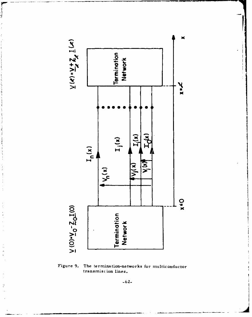
xIx

*-45 X

>1x30CI?

. ..0 0Z

>1>

Figure 9. The termination-networks for multiconductortransrnist. ion lines.

-62-

where V and V are nxl complex-valued vectors of equivalent open-circuit

port excitation voltages with respect to the reference conductor and Z0 and

2ý are n'Xn complex-valued, symmetric matrices. The linear n ports can

quite obviously be characterized by (69) and [VO] - Voij, [V ] : V as shown

in Fig. 10. For arbitrary termination-networks, the entries in (69) can be

quite easily obtained by treating V(0) and V(f1) as independent voltage sources

and writing the loop current equations of the networks. The currents 1(0) and

I(Z) will comprise subsets of the loop currents for the networks and the

remaining loop currents can be eliminated to yield (69). If the i- th conduc-

tor is connected to the reference conductor only through impedances Z0 i and

Z i, then the entries in Z0 and Z are easily obtained as [Ojjii = Zo0 i [Z 0 ]ij

= 0, [Zr].i = Zi, , = 0 for i,j = 1,---,n and i/j.

Combining (23), (25) and (69) one can obtain straightforwardly [26, 48]

us sian- - YO(,70)LZ+-'-T yle~- f'XI'YV2

Since T- Y Z T = y2 , then Y- T y in (70) can be replaced by Z T y-

Once this set of 2n equations in the 2n unknowns, I + and I -, are solved (by

GZLussian elimination and back substitution, for example, [49]) then the

response, V(x) andI(x), at any point on the line can be determined from (23)

and (25). For two-conductor lines, the matrices and vectors in (70) become

scalars and T becomes 1 (see (13) and (14)).

It is also possible to indirectly solve for the response via the matrix

chain parameters. With x = Zand x0 = 0 in (31) and (32) and using (69) one

-63-

i•',•L.,s -. . .if',;•k ,, j'-111", - • _• ,. • -. ..... b--•p ,m . " - ••

i ' \!,. I

C S

I 0 0 , 0

L..+ .- ! *I

>

t I00 ©0

I.I

Figure 10. The termLnation-networks for multiconductortransmission lines.

-64-

4-I

a.•

•. =---••. -'i: • '• .... • -'...I Oi~!#tl. - i9"i

can straightforwardly obtain [26, 48]

21() ,• •(Z) ,.V0 + 1£1.,•()Z ].(O) (71b)

where Vt., 0) Y i(. V(x) and I(x) can be obtained for any x from (8) with

1(0) from the solution of (71a) and V(0) determined from (69a). Here one

need only solve n equations in n unknowns, equation (71a), as opposed to Zn4I

equations in 2n unknowns in (70). However, certain matrix multiplications

are required in forming both (70) and (71).

Using the matrix chain parameter identities in(40), it can be shown

tha t (71) may be written in an alternate form [18]

=O )-- (72)

which has a highly sparse (large number of zero elements) coefficient

matrix with 2(n 2 - n) of the 4n 2 elements identically zero. Equation (72)

can also be solved explicitly for_1(0) andI(X) as [18]

I V - ý 20')Ji(0) +S 1 ) b (73b)

The advantage of the formulation in (73) as opposed to (71) is that only two

of the matrix chain parameters, IR, and .,g need be determined in solving

for 1(0) andI(X) via (73) (see (32)).

The most efficient method of solving n linear, algebraic equations in n

unknowns is Gaussian elimination with back substitution (LU decomposition)

-65-

which requires (n1/3 + n2 n/3) operations (multiplications and divisions)

or on the order of n'/3 for large n [49]. Thus solving (70) instead of (71a)

or (73a) requires on the order of (2n)-1/3 or 8 times the number of operations

and the complete solution of the problem requires, at a minimum, the solu-

tion of n complex equations in n unknowns. The impact of this requirement

on the overall solution times for large cable bundles can be illustrated as

follows. The time required to solve 50 complex equations with a standardI

Gaussian elimination subroutine with full pivoting (DGELG in SSP [50] which

was converted for complex arithmetic) was 12. 6 seconds on an IBM 360 /65

computer. So if it is required to solve for 100 frequencies, then the overall

computation time would be, at a minimum, on the order of 21 minutes. It

k is not uncommon to find 100 conductors in cable bundles on modern avionics

systems and since the number of operations required increases on the order

of n 3 then solutions for 100 conductors and 100 frequencies ~Vuld require,

at a minimum, 2. 8 hours! Of course, additional time will be required for

matrix multiplications (as well as the computation of Y and Z and diagonali-

zation of YZ) as indicated in (70), (71), (72) and (73). This could be quite

substantial since n 3 multiplications are required to multiply two "full" n-Xn

matrices which is precisely the number of operations required to invert an

nx(n matrix which is "full" [49].

Using the matrix chain parameter formulation in (71) and (73) has an

additional advantage over (70). It allows a straightforward incorporation of

incident electromagnetic fields into the solution. Consider (4) and (8) where

-66-

the effects of an incident field are included as distributed sources along the

line, Vs(x) and 1s(x). From (8) and (31), define equivalent sources

A A AA A A ~A_v(r) = § 1 Q ,x) _Vs(x) + ~ 2(£,x) I s(X) dx (74a)

0

A rf A) VA) A A )jdAI (') = IV() + •g 2 (£, dx (74b)

A

One can modify (71) and (73) to include these sources by simply adding I S(£)A

to the right-harid side of (71b) and (73b) and replacing V£ with V- V S(£) +

I S (S) on the right-hand side of (71a) and (73a). This is quite obvious

A

since (8) shows that for x = £ and x0 - 0, I(S) is increased byir(£) and \j£)

A

is to be increased by Vs(£) over the case without incident field illuminatin.

Fronm the boundary conditions (69b), ag=: VY£) - Z£I(£), then.V£on the right -

A A

hand side of k7la) and (73a) is to be decreased byVs(Z) - Z£IA£) and I(£) is

to be increased byIs (£) in (71b) and (73b). Thus equations (71) and (73) are

quite easily modified to consider incident fields and the final equations

become [26] a the

[z !2 (Y)- ? 02JL) zo - ,§12(•) + -01 ZoI(o) (

I. 1(.2)- S t•j(£)1 V o - V 2A A+--V (£) - zt x sI M-S -s

A

I(7) = g 1 (S') V + 10a,(£-) §21(r) Z OI](o) +Is(£) (75b1)

or [18]

[1zn - (£)) ,1 (r)o - Sa(£)}]I(0) =- Y,'(£)V£ (76a)

n iv0 k,(Z) ýý -1 ~2(y) 12 1(Z) Y-0

-67-

"" . ._M.

A A.I-S

I(:G) -- Y. *0 + [,!2 2() - §2-aP) Zo]-_(O) +-Ia(F') • (76b)

A more detailed discussion of' efficient incorporation of the boundary condi-

tions is given in [26].

The equations in (75) become particularly simple for the multiconductor

line in Fig. Za consisting of (n+l) perfectly-conducting wires in free space

illuminated by an incident electromagnetic field. It is shown in Appendix

C that (75) reduces for the case of Fig. Za with incident field illumination

to

+ .£+jsn(1 Z Z-1 7,,}]_j(O) =(77a)[cos(•, {Z•0 +Z_}+isinos£{Zc +Z _ 7_a 0L•0

V+ [j sin(Z) ZrZC + cos(s.2) i ]VO(icn-O (irnc)

+ (Z{[cos (e(8., + j sin(g. , .) ft(011)} dý

I I(inc) {[cos( Y -1n (inc(

- I(£) - j sin(B£) ZC X + [cos($£) In + j sin(B1) - ] -(

(inc) A

- Isin(a(£- x) (X) dx

-l (incIS {sin(Z) Et(o)

•'(inc) (inc) (inc)

where EE(x), E (Z) and E (0) are ny 1 column vectors with the entries in the-t -tB. i-th rows given by

(inc) (m (inc)[E (x X) E" x) - E (0.x) (77c)

$ (inc di0 (minc)-- t (ti d% (77d)

0

-68-

(inc) (1.0 (c)f .t (0)]. = ti(gi, 0) di (77&)

an0{inc) inc.for i=l,---,n io, x) and 0,i (00 x) are the components oif the incident

electric field intensity vector in the longitudinal (x) directiun along the

(inc) inc)axis of wire i and wire 0 respe'tively. The terms Eti (g', 0) and Eti (i S)

are the transverse components (lying in the y, z plane) of the incident elec-

tric field intensity vector at x = 0 and x = X respectively along the contour

•i between wire i and wire 0. The contour % is a straight-line path between

wire i and wire 0 and perpendicular to these wires. The entries $ and Z

are the wave number and characteristic-impedance nmatrix respectively

with X = v/f, v =/Fvc and Z vC = ,L. The correspondling solu-

tion for Fig. 2b is also discussed in Appendix C.

4.1 Lumped-Circuit Iterative Approximations

In deriving (4), "electrically short" &x sections of the line were con-

sidered and since the line was assumed to be uniform, all Ax sections will

be identical. Requiring that the Ax sections be "electrically short" for all

frequencies, the transmission line equations in (4) are obtained in the limit

as Ax -, 0. Alternateljy, one can construct lumped-circuit models fur the

line consisting of N identical sections of length .V'/N so that each of the sec-

tions would in itself be "electrically short", e.g., the section would be no

more than, for example, 1/10 of a wavelength long for the frequency under

consideration. Note that since f/N is assumed to be "electrically short"

and the cross-sectional dimensions of the line are assumed to be "electri-4

-69-

cally small" so that transmission line theory applies, then a lumped-circuit

representation of this portion of the line is valid. Perhaps the m)re common

models of the transmission line are the lumped-circuit iterative approxima-

tions which use this philosophy. Models are shown for (n+l)-conductor linesjIin Figure 11 as the lumped r model, lumped"? rn, .el, lumped Pi (TT) mocdel

and lumped Tee model. The lumpedIsection is similar to the circuit in

Figure 7 but with Ax replaced by IYN. The lumped I' section is the opposite,

i.e., the capacitance and conductance elements appearing at the end of the

lumped' 1 section appear at the beginning of the lumped .rsection. The lumped

Pi section is eimilar to the lumpedrlsection but has half the values of the

capacitance and conductance parameters placed at the beginning and at the

end of the sectiun. The lumped Tee section is again similar to the lumped

Isection but has half the values of resistance and inductance (self and

mutual) elements placed at the beginning and at the end of the section. The

lumped '1 model has been used in the program STRAP [361; the lumped Pi

model has been used in the program IVEMCAP [341, and lumped Pi and Tee

models have been used in power transmission line studies [9].

The 2nX 2n chain parameter matrix of a section of line of length £/N

characterized by any of the lumped iterative approximations can easily be

shown in terms of Z and Y to be (see Appendix D)

-k {}(Lumpedr1) (78a)+ Y Z(£/N) 2

[{-~u} n + J

-70Z=-7

dI

zz

01

uU

(azh leuvaetcrut

rigure 11~~. L meic i ~r tv id l fr-ilio d cu

tra sm;ssin ine (cnt

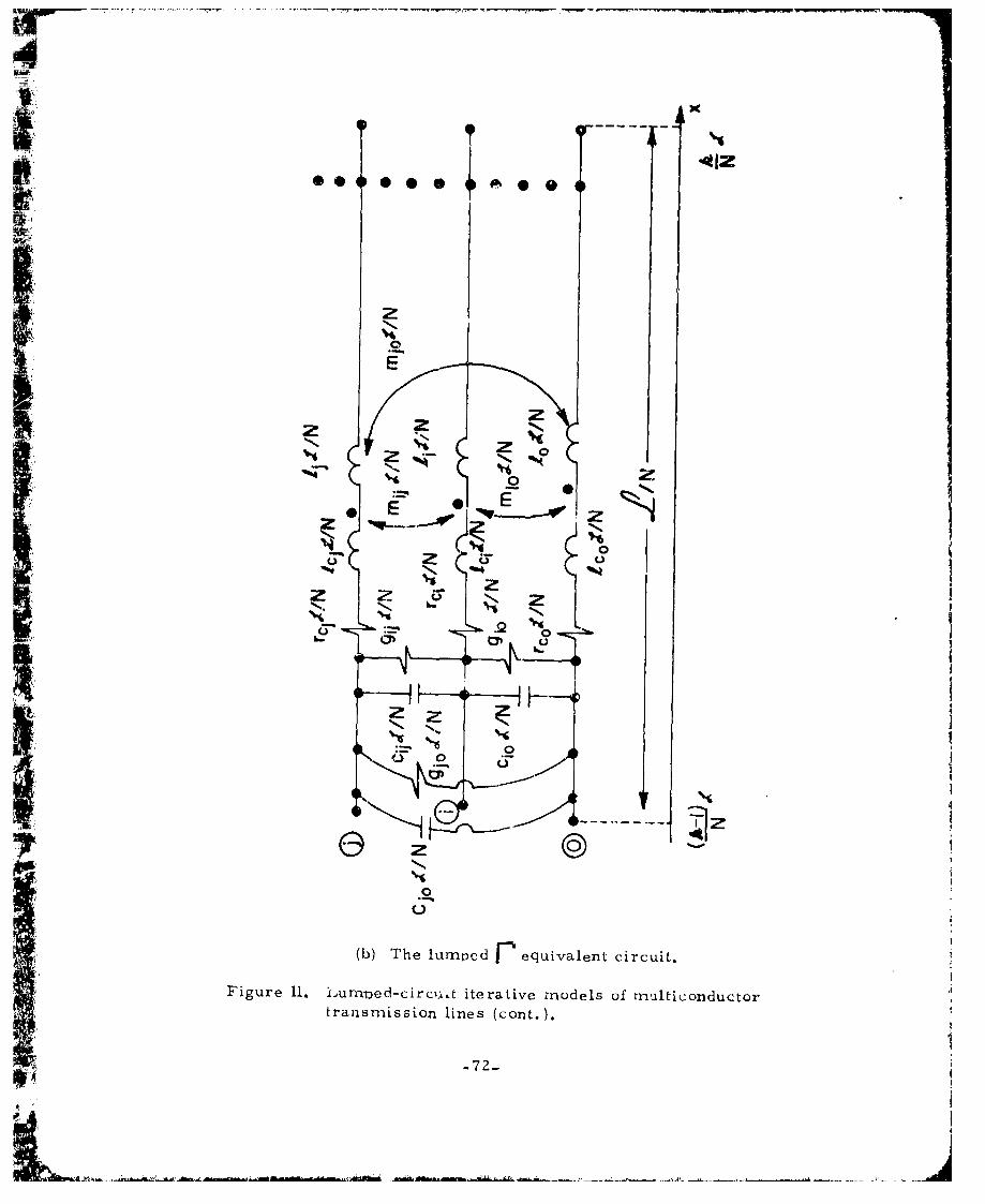
-4Z

0 0z 2

"-' - " *--- " -- .

of 2r,

00

zN z

S0ilj(b) The lumped equivalent circuit.

Figure 11. humoed-circut, iterative models of multiconductortransmission lines (cont.).

-72-01k'

UP

I0 Mzz

CI"

o~0 ©0 L0

I z(c)TelupdP euvlntcrut

-737

-Z --

D

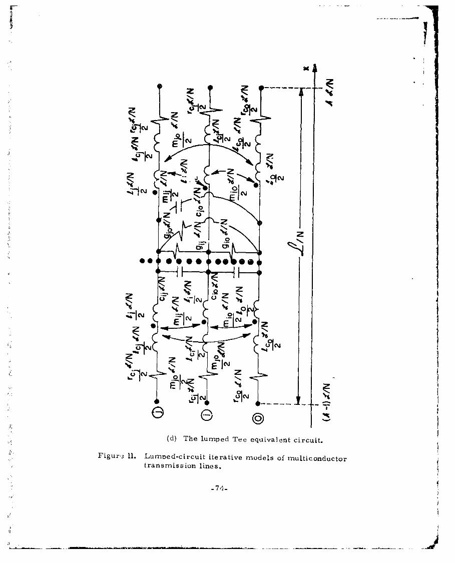
319

F 1- -

zN0

z0N

zz

L) Z'a c 0(d) h lM pe e qiaetcrut

Figur' ~ ~ ~ ~ C 11zu~dcrutieaiemdl fmliodco

transmssionlines

-7)

fl + Z YG 1 Z.},,=i /N {}](Lumped F) (78b)

n 1/2 Z Y(:/N )(} IN)

Zk Y-1 / (Lumped Pi) (78c)

Y(./N) - 1/4 Y Z YS/~ l+12YZS/

< +{- 1/,Z, Y(.,/N)2} {,Z(./N) - 1/4 Z+.,N Y )3}-k-" {-'<,,,} {f,0 1 1,2 Y'S,/N)2} J (Lumped Tee) (78d)

These models are referred to as lumped-circuit iterative approximations

since the overall matrix chain parameters for the line of length £ and N

N.sections (all of the same type) is quite obviously , ( i.e., multiply

the chain parakAteter matrices in (78) together N times, since the chain para-

meters for each section only relate the voltages and currents at the two ends

of each section as

=F t k2 ~~~79)

where each submatrix k1 1' 12kl' 2 k21' ýk2q is ny n and corresponds to

submatrices in (78) and k = 1, 2, ,N.

Generally an N section lumped-circuit iterative approximation is solved

(the boundary conditions or termination-networks are incorporated) as

strictly a lumpedelectrical circuits problem with circuit analysis jrograxyms

such as ECAP, SCEPTRE, TRAFFIC, etc. [531. The node-vottage equations

-75-

MWm

or loop-current equations of the network of N sections with termination-

networks are written and solved via these programs. It is possible to write,

for example, the node-voltage equations directly from the matrix chain

parameters without employing a circuit diagram. Using (69) and (79), one

can straightforwardly obtain (see Appendix D)

-Y 1° V(0-1 _n non. . .n V_.o) nk1 ~o-0o

A1 Y 1 0 V(£/N) n

n ~n n-n n-i

0 0

* -•n fl \ n-

0 ..... 0 1_ YN+ v(,.1,,n-,,i n - --

where

Y£= (80b)

V(N 11-Y -'LI .Z

"n~ n -lNn-

w h e r e Y (81da)

-0 -0YZ ' ,k1 2 (8Zlb)

A A

chair. parameter matrix in (79) by writing (79) from the nodal-admittance-

matrix characterizing the Zn-port and invoking synimetry of this nodal

admittance matrix via reciprocity.

In (78a), (78b) and (78c), ~k1-I = - (N/£)V and in (78d) 0k;g= f) +

1/4 Y Z (ZIN)21 {(N/Z)Z-1}. Therefore when writing the node-voltage

equations in this fashion, it appears that the inverse of the per-unit-length

impedance matrix, Z, is required. The inverse of Z is needed when

writing node-voltage equations strictly from a circuit diagram when inutual

inductances are present [53]. However, one can show from (78) that

~k2,k~~1 =tk~ (83)A

which can be used in forming Y and YN4.1 in (80) as

At

{!Lki N2 (8 4a)

Y N+1 I !k 2 Y g3t (84b)

Thus the inverse of Z is not needed when writing the node-voltage equations

in this fashion as in (80).

It should be noted that the formulation in (80) provides an additional

method of obtaining the exact, distributed-parameter solution for V(0) and

V(£). For example, taking N=l and using the distributed matrix chain

parameters 011, §, 2 §, and §2 from (31) and (32) one obtains a set of

2n equations in the 2n unknowns, V(0) and V(Y), which can be solved for the

exact, distributed-parameter solution instead of using (70), (71), (72) or ('73).

For the distributed case, one can also show,! 2 l~z1 "!21 = 1 (see (40)).

In addition, one can show that = I (see (40)) and this can be

-77-

/

used in fortning YNil in ($1). Thus, for the distributed case, j80) becomes

Iz V(O) C(.Z) Z0 V

S-- -L~ -0 -0 (85)

and (85) may be explicitly solved for V(0) and V(S!) as was done in obtaining

(73) from (72). Note the similarity of (85) to (7Z).

An important consideration in using the lumped-circuit iterative approxi-

mations is that to obtain correlation with the distributed-parameter formula-

tion described by (4) (which these models are intended to approximate), each

section must be electrically short and therefore the number of sections used

to represent the line must be increased for increasing frequency. For an

(n+l)-conductor line with N sections, (N+l)n simultaneous, complex equations

in terms of the node voltages, V(0), V(£/N),---, _V(Z) must be solved at

each frequency as is evident from (80). For N>l, i.e., using more than one

section to represent the entire line, the equations become sparse (large

number of zero entries) which is clear from (80) and the fact that each

section interacts directly with only its two iieighboring sections. This high

degree of sparsity can be used to drastically reduce the storage and compu-

tation times over that which would be required if the nodal-admittance

matrix were treated as "full" and no advantage taken of the zero entriee.

These considerations are implemented in the program, TRAFFIC [53].

Even if only one section were used to represent the entire line, i.e., N=1,

(80) shows that 2n complex equations in 2n unknowns must be solved at each

frequency. However, these equations can be solved explicitly for V(0) or

-78-

V(s) so that for N=I a minimum of n simultaneouu equations in n unknowns,

V(O) or V(Z) need be solved. In obtaining the solution of the distributed-

parameter, transmission line equations directly rather than approximating

the line with lumped-circuit iterative models, urve is also required to solve

2n simultaneous equations in 2n unknowns through a solution of (70), (72) or

(85) or n equations in n unknowns through a solution of (71a) or (73a) and the

number of simultaneous equations which must be solved need not be

increased with increasing frequency as is required with the lumped-circuit

iterative approximations.

Incident fields may also be incorporated into the solution via the lumped-

circuit iterative approximations. Define from (8)

(kZ/N) V(~~ (k-i1) Z IN1k./[ Vkk/N ](k 1).C IN ) IN)1 V5 x A

I (k9/) IN) I(( I£N) 1 -).1~/N [ W

(86)

f T(k J (k)£/N 1) 4ASfor k = 1, 2,---,N since it is assumed that (x:/N, (k-I) r

'• trically short sections, Thus, for electrically short sections, the lumped-

IF _

i• circuit iterative models can logically be modified to include incident fields

• by adding appropriate voltage and cdrrent sources to the beginning of each

7kkii.•.'.•section as indicated by (86). The r~ode-voltage equations in (80) will be

::•,.i•:modified by adding appropriate additional forcing functions to the right-hand

;J'i~iis side vector and the coefficient matrix will remain unchanged.

"-79-

[ ,-

The question of convergence of the lumped-circuit iterative approxi-

mations to the distributed-parameter solution is difficult to answer quanti-

tatively. A preliminary indication can be obtained by observing the con-

vergence of the overall chain parameter m-atrix for an N section represen-

Ntation, *k to the distributed-parameter chain matrix (or state transition

matrix), 0. The state transition matrix f(S) (equations (31), (32)and (33)

with x = £ and x0 = 0) can be expanded into an absolutely convergent

infinite series as shown in (34) as"(87)

n n-n 'F -n-n, +C3 +

Expadi-th++ ~- -

Expanding the chain parameter matrices for the lumped iterative approxi-

mations in (78) one obtains for the lumped mo nodel:

Lln1 1 n Ln~

n nn n-n . ~-n n-n

Zk 0% 1 -Y 0 0 Y z

n-n -a n n-n ondn

and for the lumped Te model:

1 0 z Y 0

nk n n 1 [ 0] n n,-njN

4 (88b)

0 0n-n 2n, L- n- n.n n -n,and for the lumped Pi model:

1~ 0-n ~ ,n (8 8c)~nnn+[10 Z/() Y-~ nn 1/2(X)3

0l~ 1~J- JN0.+[ N LYZYO0 N

and for the lumped Tee model1:

-80-

I-k n Z ~n] -Xn~ [1/4(- n-

(88d)

Note that for N 1. i.e.. one section is itsed w represent the entire lint.

the lumped Pi and lumped Tee models appear to be better approxim.tions to

the distributed solution. V(1) in (87) than do the lumped T" and lumped r1

models in tP sense that the first three terms of (88c) and (88d) are identi-

cal with tWe first three terms of O(P) and the fourth term is only partially

the fourth term in §(2). In the expansions (88a) and (88b), only the first

two terms agree with the first two terms of O(Z) and the third term partially

agrees with the third term in §(1).

There are c•trtain other lumped approximations which at first glance

seem to be not included in this discussion but are, in reality, versions of

J lumped-circuit iterative models using only one section to represent the

entire line and with certain circuit elements neglected r35]. In addition,

with these approximations the rapacitivo and inductivp coupling are cornx-

puted independently of each other and added together which is generally only

valid for weakly-coupled lines (see reference 130], pp. 287-291).

LI

-81-

V. THE PER-UNIT-LENGTH PARAMETERS

Derivations of the per-unit-length parameters of internal resistance and

internal self inductance, i.e., the entries in Rc and L., which account for

skin effect associated with imperfect conductors are well known for solid,

round-wire conductors and are found in numerous texts r2, 3, 301. These

internal parameters are derived by assuming that the currents internal to

the conductors are symmetric with respect to the centers of the conductors.

However, for closely-spaced conductors, this assumption may not be valid

since proximity effect can alter the internal current distributions (see

reference r4 0 ], Chapter 9).

The de 'vations of the per-unit-length external parameters, i.e., theIi~l'entries in G, L and C, assume all (n+l) conductors are perfect conductors

and are more involved especially for close conductor spacings. These

parameters generally only exist in closed form for the simple cases of two-

conductor lines in homogeneous media in Fig. 4 consisting kf two bare wires

in an infinite, homogeneous medium in Fig. 4a (reference [55], pp. 133-136),

one bare wire in an infinite homogeneous medium above an infinite ground

plane in Fig. 4b (reference [55], pp. 183-185), and one wire within a circu-

lar shield which is homogeneou,,y filled with a dielectric in Fig. 4c (ref-

erence [55], pp. 125-133).

Having accurate values for the entries in the per-unit-length parameter

matrices, especially the external inductance arnd capacitance matrices L and

C, is obviously important in obtaining accurate solutions and the per-unit-

*: -82-

lengt.h pa r.t nieters nust bhe old)ainfed evn when using lflu)ed-( ircuil iteret-

tive appr(iximations discussed in Section 4.1. It is important to remember

that with the assumption of TEM modc propagation on the line, the trans-

verse fields at each x along the line satisfy a static distribution and there-

fore the per-unit-length external parameters, i.e.o, entries in G, L and C,

are obtained as the solution to a two-dimensional static fields proble'n [39].

This also is implied in the inhomogeneous medium case under th. "quasi..

TEM mode" assumption.

5.1 The Per-Unit-Length External Parameters for Lines in a Homogenutmui

Medium

The per-unit-length parameter matrices, C, Land G for lines imrmers-

ed in a homogeneous medium possess the important properties given in (44),

LC = CL= ui and LG = G L =ual . It can be shown 154] that, for an_ -4 1,

homogeneous medium, each of these matrices is related to an nXn nmatrix,

K, which is independent of the parameters of the medium and dependent'0

only -,n the cross-sectional structure of the line as

C =cK (89a)

G " K - (a. /e) C (89b)

L uK e C1 (89C)

For two-conductor lines in a homnogeneous medium, the per-unit-length

parameters in the transnmis ,ion line equations in (1) ar,. obtainable, exactly

in closed form even for close conductor spacings where proximity effect

produces a nonuni"uorm charge distribut:ion around the conductor peripherios

155]. The rr-atri. •( in (89) becomes a scalar K and the parameters in (1)

-83-

Arm

become c eK, g = IK, = uK

For two wires in a homogeneous medium in Fig. 4a, the per-unit-length

capacitance becomes [56]

Crr (90

cosh 1 (d"a - ra,- r2)/(Z rwi rw (90)

For widely-separated conductors, (90) can be approximated by [31

2cT C -(91)

\r 1 r• ,

where in is the natural logarithm. For identical wires with rwl = rw0 = rw0

(91) yields less than 5% error for (d/rw) > 5 [55, 56]. For the case of one

wire in a homogeneous medium above an infinite ground plane as in Fig. 4b,

the per-unit-length capacitance becomes [55]

C 2rr E: (92)cosh"1 (h/r

and for (2h/rw) > 5, (92) can be approximated by [55]

c Z e" (93)

For the case of one wire within and centered on the axis of a circular shield

which is homogeneously filled with a dielectric as in Fig. 4c, the per-unit -

length capacitance becorr'•s [55]

C2r c(94)'n (rs /rw)

In all of the above cases, c = K and K is easily identified. In addition,

I uv K' and g = aK. For Fig. 4a and Fig. 4b, e= v and c= 0.

-84-

IThe p'irarneters for lines consisting of more than two conductors are,

in general, not obtainable in closed form for closely-spaced conductors and

numerical approximations must be used. These techniques generally fall

into two classes; the methud-of-moments techniques [56-62, 22, 66.-68] or

ini.ging techniques [63, 64, 65]. A particularly successful technique is the

use of harmonic expantion functions to describe the charge distribution

around the conductor peripheries [56, 57].

Consider the system of (n+l) bare wires in Fig. 2a. With the moMent

method using harmonic expansion functions, the free-charge distribution,

around the cross..sectional perime ter of the i-th conductor por unit of

length in the x direction is described as a Fourier series with respect to ai

cylindrical coordinate system at the center of the i- th conductor as shown in

Fig. IZa, i.e.,

A i Bi

Pi (0j) = ai0 4. ait cos Ynf9, + T b sin 111 (95)O , 1,---,n.

The absolute potential, 0 (rp, S.), at an arbitrary point P located at aP p j

radius r and angle p shown in Fig. 12a due to this charge dist ribu(ion over

the i-th isolated conductor is [56, 57J

13(r {ajO I1d (lei ,(96)

Ai •27r 13i 2rr+in aim 0 cos(rnei) I((t + 0sin(

1. The tert-n "absolute potential" re'ors to the potential with vespect to infin-ity and the reference potential ternis are oinitted in (96). 'liiis is validi"for a system with zero not charge and is demonstrated in Appcondix E.

•) -85-

The parameters for lines consisting of more than two conductors are,

in general, not obtainable in closed form for closely-spaced con luctors and

numerical approximations must be used. These techni ques generally fall

into two classes; the rmethod-of-moments techniques [56-62, 22, 66-68] or

imaging techniques [63, 64, 65]. A partkculai ;uccessful technique is the

use of harmonic expansion functions to describe the charge distribution

around the coiiductor peripheries [56, 57].

Consider the system of (n+l) bare wires in Fig. Za. With the moment

method using harmonic expansion functions, the free-charge distribution,

pi. around the cross-sectional perimeter of the i-th conductor per unit of

length in the x direction is described as a Fourier series with respect to a

cylindrical coordinate system at the center of the i-th conductor as shown in

Fig. l2a, i.e.,

Ai Bi

pi (0i) = a + E aim cos mei + F b. sin nmP (95)m=l m=l IT i 0: 1,,-- ,n

. 1

The absolute potential, p (rp, a }, at an arbitrary point P locared at ap p

radius r and angle 0( shown in Fig. 12a due to this charge distribution k, vc,Sp

the i-th isolated conductor is [56,5712T,

tp(rp, ep) =- 4r,---a-• o

Ai 2('TT i2+ >2 aim cos (m ai) I (0i) dO. + F' b. sin(m Ei) I(il (dBim=l m 0m im j

1. The term "absolute potential" refers to the potential with respect to infin-

ity and the reference potential terms are omitth-d in (96). This is valid

for a system with zero net charge and is riemonstrated in Anpendix E.

-85-

~1

#P P

i - th conductor 4r

rwi

(a) (

I

S"---8 i (ri

/* "i c , 'C 9PP I

(b)

Figure 1Z. The geometry cf the charge distribution problem.

-8M-

where I(O) t,') ,. ri. - rp rwi cos (Ei - 6F)4rwi. [h. , inte. r-IlI- W1 p

can be evaluated in closed form yielding 156, 571 (See Appendix E

(e+ 1)

, - tr n (r ) Ai rw. cos(me

(r = -a(+ ai Zmr / (97)

p(m+l)

Bi r * sin(me+ b.

m=1 im m. rm

p

Associated with each conductor in Fig. Za there are A. + B. + 1 un-

knowns; the expansion coefficients a 0 , a i b. in (95), These unknowns

will be determined by enforcing the boundary conditions that each conductor

(including the reference) is at an absolute potential ,i, i=0, 1,---n. A total

nof E (A. + B. + 1) match points will be chosern on the (n+l) conductors at

i=O I

which the potential due to all charge distributions in the system (including

the charge distribution on the conductor associated with the match point)

nwill be enforced. This results in a set of 'E (A. + B. + 1) equations in

the same number of unknowns and can be written as [56, 57]

P P= 5 (98)

n

where p is a vector of length *7 (A. + B. + i) containing a 4 of the unknown

expansion coefficients aj 0 , aim, bhn and OS is a vector of the assumned con-

ductor potentials as

-87-

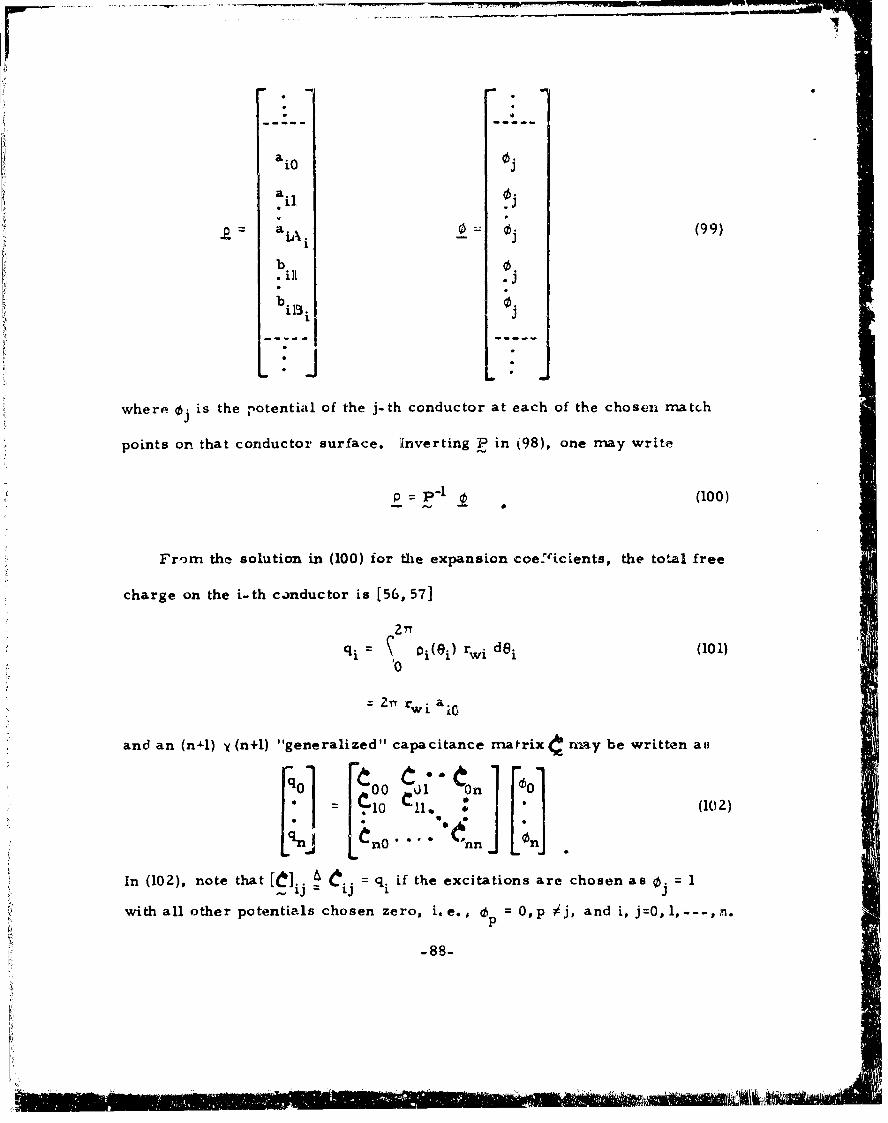
a0 0 j (99)

b

b 0~

points on that conductor surface. Inverting P in (98), one may write

P P-1(100)

From the solution in (100) for the expansion coe-'iclents, the tot.al free

charge on the i-th canductor is [56, 57]

2TY

Fl .

1 . .1 r Ii [8n1 (10•)

b ~ ~Zi ,we a m e

in(0 no e that [cndct su "geeralzed taep citanti ons are mchenay wriaten

10 11.I• (IOO)

In(0r) om the sution t n q0 ifo the exciansions are choentasteotlfe

1j 3

with all other potentials chosen zero, i. e. , b O,]p ij, and i, j=0,

-88-

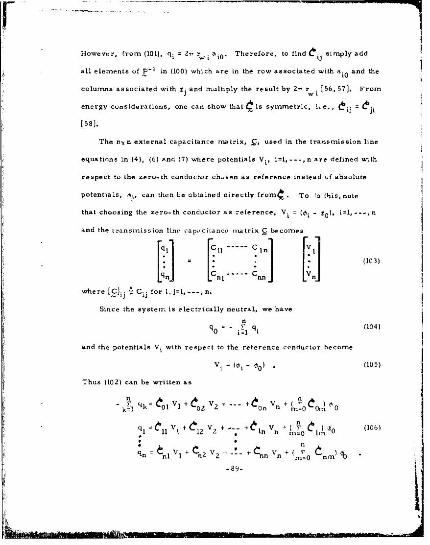
However, from (101), qi = 2r r ' a. Therefore. to find .ij simply add

all elements of P-1 in (100) which are in the row associated with a. and the

colurmns associated with tj and rrmultiply the result by 2,- rw [56, 57]. From

energy considerations, one can show that iis symmetric, i.e., ij =&ji

[(58].

The nyn external capacitance matrix, C, used in the transmission line

equations in (4), (6) and (7) where potentials Vi, il,---,n are defined with

"respect to the zero-th conductor chusen as reference instead uf absolute

potentials, ej, can then be obtained directly fromil. To !o this, note

that choosing the zero-th conductor as reference, Vi (0i - 00). i=l,---,n

and the transmission line capicitance tm-atrix C becomes

11 i(103)

Sinenhe' [.nI l ~ n LVnJ

where [C].j : cj for i, jl, --- ,n.

Since the systerr, is electrically neutral, we have

n- n (q04)

and the potentials Vi with respect to the reference conductor become

V. : (0.- 0) (105)

Thus (102) can be written as

- q 4 k 01 Vl +6 0 1 V2 + +e'On Vn +( _ C' •o

ql:'I Vt +Cl 1 V2 + +J& ± nVn-7(rn O'l (106)

* a

nl I n2 V2 nin n0

-89-

/A

Adding all equations in (106) together we obtain

or n n n

W.0 - v iv+Q'c )v2 + -- + U~~f (107)

1~~i- on- ml 1U r2) z(.V

or in (-"0nn~l ~i~0n (108)1

n si0 c tr an

+ F- (F tnt ( 1 0

or~i [J (m =0 ~ m i - M= I ~ m

Noetuatios[ the dforrmnao of (103 ) y ie s ml the sutrifsall the ee-ntle engtht ns -o!

Theio lnueraatoroa (0)c anri bewite as ,nn n

Ci~ L,~o inko [(mJ ,=j (\ Ornk >i k1% m)(10

-0 n n (108)

I '

Noe that-osi the f~onnorm of (1039) y ie s s l the entriesain the ee-ntle enghtrans-

misio line capeactanc mari C19 c a s ewitna

rm~j rn/i

M= -90-

ij ij. n noII .

*

= M

-w ~ ~~~ ~~~ E•--••• • • "......m-.-..

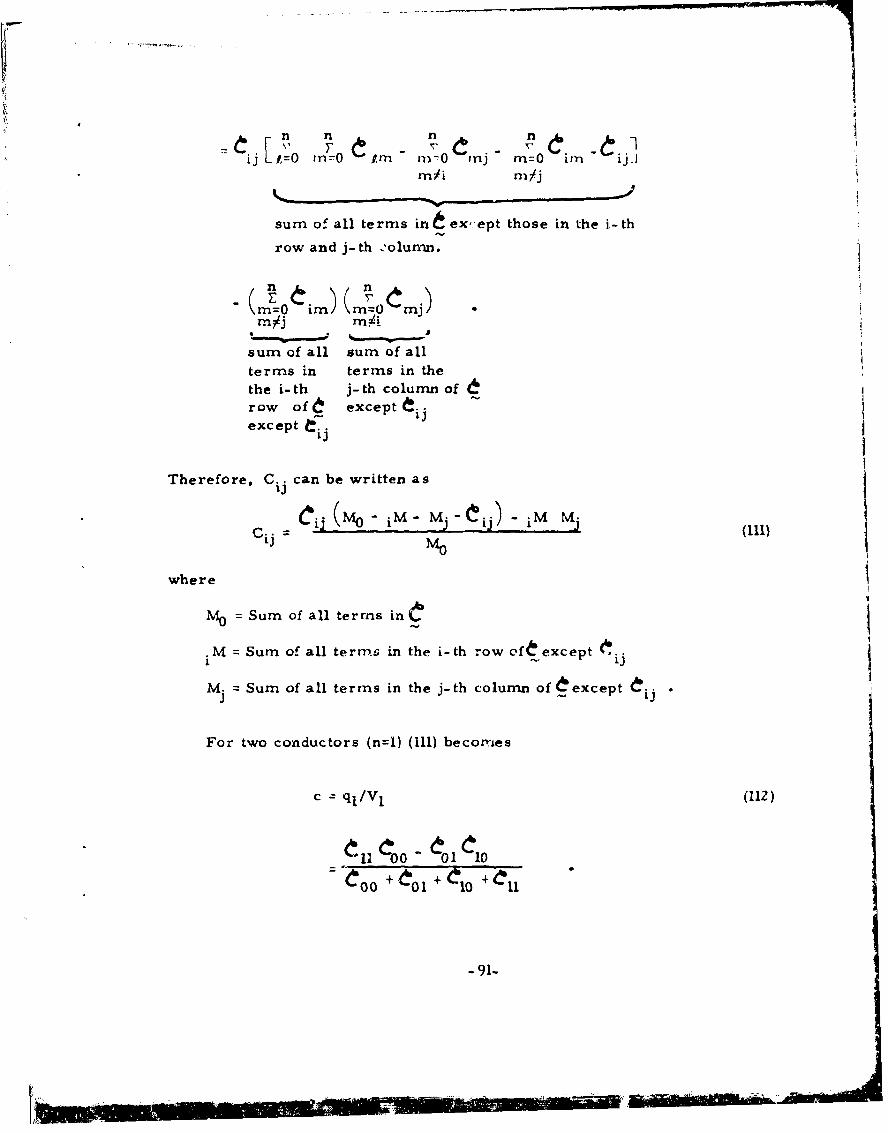
in n n n

"ij L/,0 --.O -- ,rn -M -O inj m=O irn iji1rnmi rn/j

sum of all terms ini ex,.ept those in the i-th

row and j-th column.

(n 0rn)(m O j) ( 6(rn;4

m Jj MA

sum of all sum of all

terms in terms in the

the i- th j- th column ofrow of I& except d..

except Oij

Therefore, C can be written as

C= 1 IV -i ij M M. 11Cij=

cij -MO

where

M0 Sum of all terms in

M Sum of all terms in the i-th row oft except ij

AM. Sum of all terms in the j-th column of &except •

For two conductors (n=l) (ill) becomes

c ql/Vl (112)

tll00 ÷ 01 10l +l~oo+ 'to, + Clo +e 11l

-91-

-MIS

S~This result for n--I is also obtained in rof•erence 1581, pp. 211-213.

This numerical technique can also be applied to the systems in Fig. 2b

by replacing the ground plane with the conductor images having equal but.,1

opposite charge distributions. As an example, consider the system of n

bare wires above an infinite ground plane in Fig. 2b. Replacing the ground

plane with images results in Fig. 13. Note that the oriezitation for 8. on the

image of the i-th conductor is the same as the orientation for ei on the i-th

conductor however, the charge distribution on the i-th conductor image is

-p. (-8.). Also, note that the potential of t.he i-th image conductor is taken

to be - 0 By symmetry and the use of image dietributions, the voltage of

the i-th conductor with respect to the ground plane, Vi, is equal to 0 since

iithe potential di'ler'ence between the i- th conductor and its image is 6•i-(-),

20i. Therefore, we only need to enforce the potential iat match points on

the n conductors above t.Le ground plane due to all charge distributions in the

system (those on the n wires and on the n image wires). Thus a set of

nA, i~l (Ai + B. + 1) equations can be written as in (98). However, these equa-

tions will differ from those in (98) in that the expansion coefficients for the

zero-th conductor (the ground plane), a 00, a0m b will not be included

"in the vector P and the potentials 60 will not be included in the vector 0n n

These vectors will be of length E (A. + B, + 1) instead of T (A. + B. +1).iz=1 I i0 =

Furthermore, we may replace 6i in ( by V1 . Inverting P we then may obtain

the entries in the transmission line capacitance matrix directly without the

need for (11) since V. ,V. Therefo're, C.. is simply the sum of all elements

lift,

2..1

rwi

hi~

:iV r601

vi0-1 h-2jrwj

IlkI!:\/ I I/ \

:i+ - •(-O, \\ /

IhL.L

Figure 13. Malticonductor transmission tines above e- ground Diane

ari the use of image distributions.

-93-

NOW___-,-

:''I

in P1which are in the row associated with ai and the columns associated

wi ch o. = V. multiplied by 2rrr .for i=l,---,n and j-l,---,n.

Consider the case of n wires within a circular shield shown in Fig.. 2c.

Rather than imaging the conductor charge distributions across the shield

boundary, one may expand the per-unit-length free-charge distributions

around the n conductor peripheries in a Fourier series and also expand

the per-unit-length free-charge distribution around the interior periphery of

the shield. Note that in this case, the voltages of the n wires with respect

to the sh;.eld, Vi, will be Vi = Oi - 00. Thus Ill) can be used to obtain C.

Note that for all these cases, once qis determined, L and Q are

obtained through (89) as L =uve ,.1 and G = (ale) C. For Fig. 2a and

Fig. 2b, E = ev and a = 0.

It is also possible to obtain closed-form approximations for Q, L and

under the assumption that the conductors are widely spaced and these

formulas represent the predominant method of computing the entries in

these per-unit-length matrices [55, 57]. If it is assumed that the wires in

Fig. Za are sui~iciently separated so that the charge distributions around

the wire peripheries are constant, i.e., proximity effect [55, 56, 57, 58]

is not a factor, then only one expansion function is needed in (95), ai 0 . In

this case there are only (n+l) unknowns , aj0, i=0, 1,---, n. Further-

more, since the wires are assumed to be widely spaced, then rp in (97)

can be taken to be dio, dj 0 or dij, whichever is appropriate, when compu-

ting the contribution to the potential of a conductor due tn the charge on

.- 94-

41

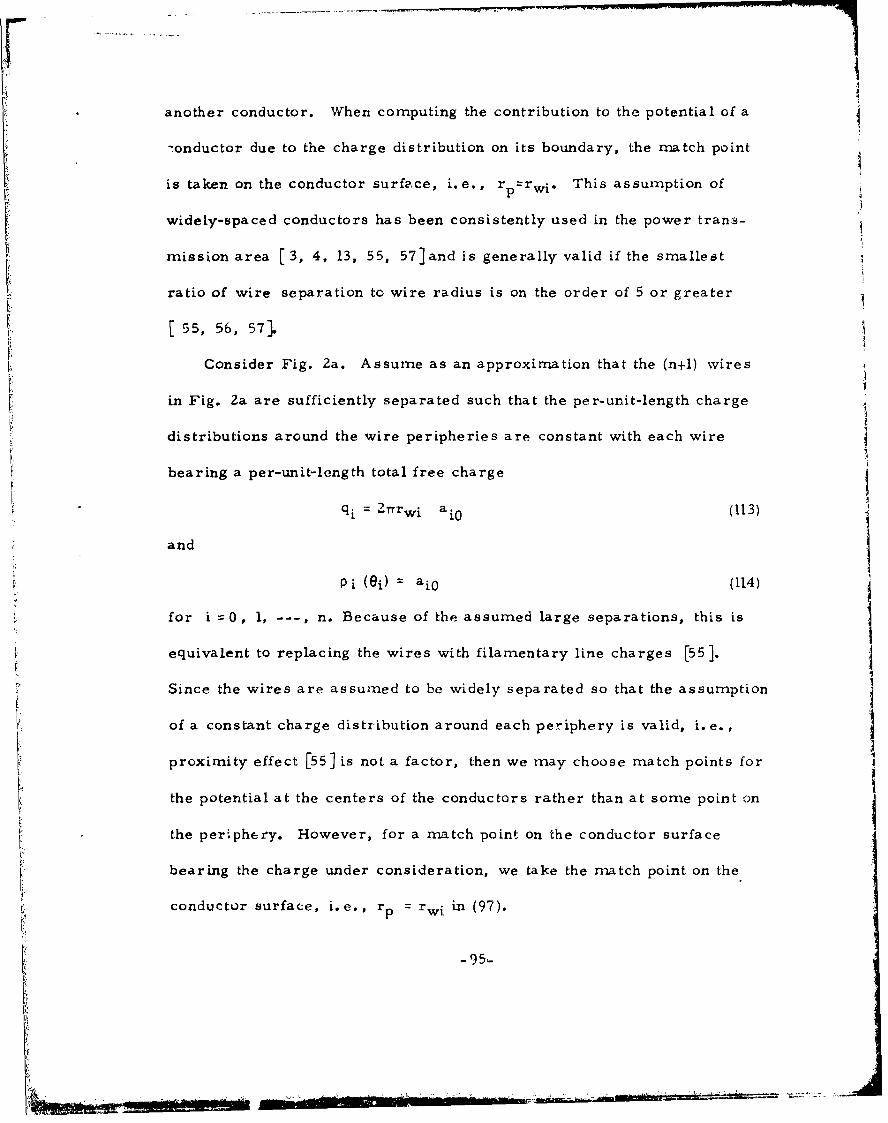
another conductor. When computing the contribution to the potential of a

-onductor due to the charge distribution on its boundary, the match point

is taken on the conductor surface, i.e., rp=rwi. This assumption of

widely-spaced conductors has been consistently used in the power trans-

mission area [3, 4, 13, 55, 57]and is generally valid if the smallest

ratio of wire separation to wire radius is on the order of 5 or greater

[55, 56, 57].

Consider Fig. 2a. Assume as an approximation that the (n+l) wires

in Fig. 2a are sufficiently separated such that the per-unit-length charge

distributions around the wire peripheries are constant with each wire

bearing a per-unit-length total free charge

qi 2rrwi a.o (113)

and

P i (ei) = aio (114)

for i =0, 1, --- , n. Because of the assumed large separations, this is

equivalent to replacing the wires with filamentary line charges [55].

Since the wires are assumed to be widely separated so that the assumption

of a constant charge distribution around each periphery is valid, i.e.,

proximity effect [55] is not a factor, then we may choose match points for

the potential at the centers of the conductors rather than at some point on

the periphery. However, for a match point on the conductor surface

bearing the charge under consideration, we take the match point on the

conductor surface, i.e., rp = rwi in (97).p '

NEW -

From the previous results and (113), we may then write (utilizing the

first term in (97))

>1--(115)

€0 Pn(rwo) tn(djo)•. 0 .*n(dn 0 ) q0ml •n(dlo) In(rw, ) n(dl2) q Il,

Applying (105) to (115) results in a typical equation

= ~InZ• { :n/i-L- q0 +'-4 Inll0 (:-0rwi qi (116)

S- - -0-d- d n

0 0 0

Aorppl ing (105) to (15) resus idtya

Vi = I .=n qrw+rwO (117)

+ n q%(1rw16 d j ( Inb)

- - U- i +Ln =n~ q+ + idin\ n

,4dwo)

for i, j=1, - . .---, n.

-96-

•-•; .; ._ .,.i_ _.:__.•il_ ' • 7 -iii:i=' : : '< ' + ...... 2 n ÷w i' w +-":•# .... -:•';l..- (117)::; :.. . ,::•-• ••:L •... ,;-,,;... . .i- •, " .,:•..: •• .. :"

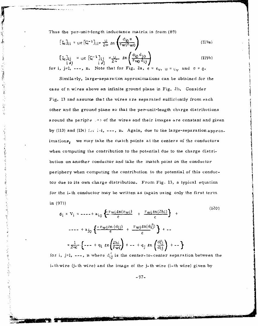
FIThus the per-unit-length inductance matrix is from (89)

[Mii =ue [Q- 1]ii Inriw) fa

[0 u[Q -IL- In (119b)i 1j •.'rrr

for i, j-l, --- , n. Note that for Fig. 2a, e = ev, u uv and a = 0.

Similarly, large-separaltion approximation.- can be obtained for the

case of n wires above an infinite ground plane in Fig. 21. Consider

Fig. 13 and assume that the wires are separated sufficiently from each

other and the ground plane so that the per-unit-length charge distributions

around the periple ,: of the wires and their images are constant and given

by (113) and (114) t-Jk -,i, --- , n. Again, due to tne large-separationapprox-

imatione, we may take the match points at the centers of the conductors

when computing the contribution to the potential due to the charge distri-

bution on another conductor and take the match point on the conductor

periphery when computing the contribution to the potential of this conduc-

tor due to its own charge distribution. From Fig. 13, a typical equation

for the i-th conductor may be written as (again using only the first term

in (97))

"- - - - - - - -- - {rwitn(rwi) + rwin(2hi)} + (120),, i=Vi a-i + ai0(2 i) +

L- r' rwj ýn (dij

.aj 0 _{rwit (dij) + ij 4-

+ q n- +-- +qn - --Zrewi,)+-- I dij

for i, j=l, --- , n where 26. is the center-to-center separation between the

i-thwire (j-th wire) and the image of the j-th wire (i-th wire) given by

-97-

.. "• J _ __ ,,2

d. + 4 hihj

Comparing (120) Wo (103) and using (89), we obtain

~1

[IL] - U Eh: hQ 2 U In 2 (121a)

EL [c- E: (122 b)i ij Vj _n i j L

for i, j=l, --- , n. Note that for Fig. 2b, F,=cv, u =uv and a= 0.

Large-separation approximations may also be obtained for the system

of n wires within a circular ahield in Fig. 2c. We assume that all n wires

are sufficiently separated from each other and the shield so that the wires

-ay be replaced by filamentary line charges. The circular shield

(assumed to be perfectly conducting), may then be replaced by filamentary

line charg3 images. Each filamentary line charge has an image on a

line joining the line charge and the center of the shield and is at a din-

tance of rs/ri from the shield center where rs is the shield radius and

ri is the radial distance of the i-tn wire from. the shield center [58]. One

can then straightforwardly derive, by superposition

In I (12 3a)[•'l~ qi q-1" ___,-- qi-1, qi+l,-' qn= 0

= I rn ( r s r 12

,j j- ' I qj+l" q = (123b)

1 - T 1 rir i)2 + rJ 4 - 2rirircosj=FT rij' + rj' - Zrirj3 o' e

where Bij is given in Fig. 2c.'=• - 9,3-

I98

..............

F!To derive (123), consider an infinitesimal line charge of radius r

w

bearing a total per-unit-length free charge q. The potential at a point

r >r with respect to the line charge surface as reference is (see reference

[58], page 92)V =)n (124)

2rrev

Equation (123a) can then be derived from Fig. 14a with (124) and q.z- 0 asqi i r__ r_ _

q. (r2/ ri-r ) /,r2 JrLrs fr- r\)

V -- I Ln (-r§ rI -n (Irn) + Sn Wi/r ~ i wi

q .Cv (125)

Equation (123b) can be derived from Fig. 14b by making use of the result in

(124) and the law of cosines. With qi= 0, we obtain

,,d 2d22 _s_

Vi 1 , ( dld 1 1

•In d2=r + s/j An ri/j cIn •Ij (17b

" r(126)

2TTev 2 d

Utilizing the law of cosines, one may obtainj

(r s

d 2 r 2 + (r~i 4 2 -r ) (2r rirj) COS (127b)2 2 S2 \2 /d r.. + (2r~ r) Zrr/ cos i (127b)

S: r2d = r 2 + r (2rir.) cos Oij (127d)

Substituting (127) into (126) yields (123b).

"-99-

r

ti

i C-4 IIIV -

C'I

Figure 14. The replacement of the wires ard the shield withinfinitesimal line charges for shielded, multicon-ductor lines with large separations in homogeneousmedia.

- 100-

IA m 11lm m

5.2 The Per-Unit-Length External Parameters for Lines in aa lnhonio-geneous Medium

Derivations of the entries in G, I. and Q for the lines in Fig. 3 are

complicated by the inhornogeneity of the surrounding medium introduced

by the interface between the dielectric insulations aihd free space. The

inhomogereity is introduced through the permittivities and conductivities

of the insulations since the dielectric insulations are characterized by

free space permeability, Uv. Therefore, the per-unit-length external

inductance matrix, , can be found as L=uv C where C61 is determined

as in Section 5. 1 with the dielectric insulations removed and may be ob-

tained accurately with moment methods and harmonic expansion func-

tions or may be approximated for large conductor spacings by (119), (122),

or (123).

The computation of the entries in Gintroduces some conceptual dif-

ficulties for the inhomogeneous medium cacc.. Consider the computation of

Sfor static excitation (reference F391 Chapter 6). The transverse con-

duction current density ;T, is related to the transverse electric field,

9T, in each dielectric as =T =di •'T. The boundary conditions on the

potential function (A where PT = -grad 0, is that •tanmust vanish over the

conductor surfaces (perfect conductors are assumed for this computation)

and the derivative of Onormal to the dielectric-free space boundaries

must vanish at the boundary (see reference F391 chapter 6). The latter

requirement insures that the normal component of ;T is zero at ,aese

-1I01-

boundaries, i. e. no current flow into the free space nredium. The con-

sequence of this is that if none of the dielectric insulations touch each

other or the ground plane or circular shield, then Qcomputed for static

conditions with a straightforward applicat'on of the above boundary con-

ditions would be identically zero since no conductive path between the

conductors would exist for nontouching dielectrics. However, dipole

relaxation effects will nevertheless produce certain losses even for a

transverse field distribution and nonstatic excitation since the trans-

verse displacement current will have a portion in phase with the transverse

electric field. Therefore, equivalent shunt conductarAces should be de-

termined to represent these non-static losses.

Assuming perfect dielectrics, however, one can compute the en-

tries in C in a straightforward fashion. A moment method of solution

with harmonic expansion functions as in Section 5." can be used for this

problem [56, 57] Consider the system of (n+l) dielectric-insulated

wires in Fig. 3a. Represent the bound-charge distributions at the di-

electric-free space botndaries with Fourier series as [56, 57]

A A

Ai A Bi APL 09d = li0 + E a ir cos m~i + r bim. sin m~t(18

~i~a +~am c i=0, 1, --- , n.

Represent the charge distributions at the conductor-dielectric boundaries

(which is total charge, bound plus free for this case) with Fourier series

as in (95). The contributions ýo the potential and electric field at a point

P in Fig. 12b due to each of the components of the charge distributions

are given in Table I with respect to Fig. 15 [56, 57].-102-

TABLE I

Contributions to the Potential and Electric Field at a Point P in Fig. 15

due to Harmonic Expansion Functions on a Circular Boundary.

Expansion Contribution to the Contribution to theFunction Potential at P Electric Field at P

rb ln(ru) rb- _ _ _r

ev evrp

(re+l) /r) m+l

Cin m91 (b bn /~ 2 ,, Lsi+sin rnkg

(re+l) rp+lsin m Ob rb sin ms (rb,/ lts)in m(9,) r

2ev rn r " 2 ev f-cos Mr1p

(a) rp > rb

Expansion Contribution to the Contribution to the

Function Potential P Electric Field at P

1 rb Zn (rb) 0

ev

r M COS rr•,, (rp/rb)rn- .rn cosn-Icos mcb Z svrn (r b)m_ 2(v f

-sin me"6(

2 e•, m(rb) ;- 2meDrv +Cos ME

(b) r <rb

)-i --0--

--.. -q . .. ... . ... - e n• -L-- J--. ~ - -: • - --- - In nI. - * I I , . P I il m Iq n

INI

cicub' bmw~ary

{COS MObi

Figure 15. The geometry for Table 1.

-104-I

J

A AThus there are 2 + A. + B. + Ai + B. unkknowns associated with each

I I

A A Awire, aiO, aim, b aio, aim, bim. The boundary conditions will be

enforced by requiring that the potential on the i-th conductor due to all

source distribitions be dq and the normal component of the displacement

vector due all source distributions be continuous at the dielectric-free

space boundarie~s. Generally I+Ai + Bi match points are selected on the

A Ai-th conductor and I + Ai + Bi match points are selected on the interface

between the i-th dielectric and free space. The component of the total

electric field (from all source distributions) normal to and just i-side

the Iielectric-free space surface at each match point on this surface is 4

multiplied by ci and set equal to the product of ev and the component of

the total electric field (due to all source distributions) normal to and justn A Aoutside the boundary at this match point. A set of .30(2 +A, + Bi +A, + t•)

simultaneous equations can be written to enforce these conditions as

[56, 57]

LP L----- L(l (19)

where .1•and are defined in (99) and 2is a column vector of the expansion

coefficients in (128) arranged as in p and 0 is a colurrm vector of zeros of

n A A

length 57 (1 + Ai. + Bi).1=0

Inverting Q in (129), one can obtain [56, 57]

L~i Li pj(130)

-105-

zJ15

L.I

The total free charge on the i-th conductor (which defines the general-

ized capacitance matrix) is given by [56, 57]

qfi = qi + qi= P (0i) rwi d0ý + S i(1(6) (rwi + ti) d~i (131)0 0

Z-rwi a 0 + 2-r (rwi + ti )aj0

since qi is the total charge at the conductor-dielectric boundary which is

the sum of the total free charge and bound charge with the bound charge

being identical in magnitude but opposite in sign to the bound charge on the

dielectric-free space suirface, 4i, i. e., qi = qfi - 4i, and ti is the thick-

ness of the i-th dielectric. The generalized capacitance matrix can be

written as in (102) where qi in (102) is replaced by qfi from (131). By

using the excitation dj = 1, Op O,p ij, [!t]ij equals the sum of two terms.

One term is 2r rwi multiplied by the sum of all elements in P'- which are

in the row associated with ai0 and columns associated with 6j and the

other term is Z2T (rwi + ti) multiplied by the sum of all elements in F.7

which are in the row associated with Ajo and the columns associated with

Oj [56, 571 The entries in the n xn per-unit-length capacitance matrix, C

used in the transmission line equations can then be straightforwardly ob-

tained from the (n+1) X (n+l) generalized capacitance rair,, C&, as in

(111). 1

Typical computed results for two dielectric-insulated wires ai.

shown in Fig. 16. By symmetry, the coefficients of the terms in (95) a;a.:

(128) are zero, i. e. bim = 0 and =im 0. Therefore the expansion func-

-106-

0I

E -

SI + Dlictric - rFm SpaceS, Coundtry •jBoundary

Mi~.Er 3.0, rw1, LOtaI.O

z1

0.00 90.00 60000 270.00 36.000

9 (Degiees)

(a)*1

* Dielectric Present+ Dielectric Removed

0

4 0

0

0010.00 5.00 10.00 15.00 20.00

Number of Exponsion Functions Per Boundary

(b)

Figure 16. ComTouted results for two dieleztric-insulated wires.

-,107-

all

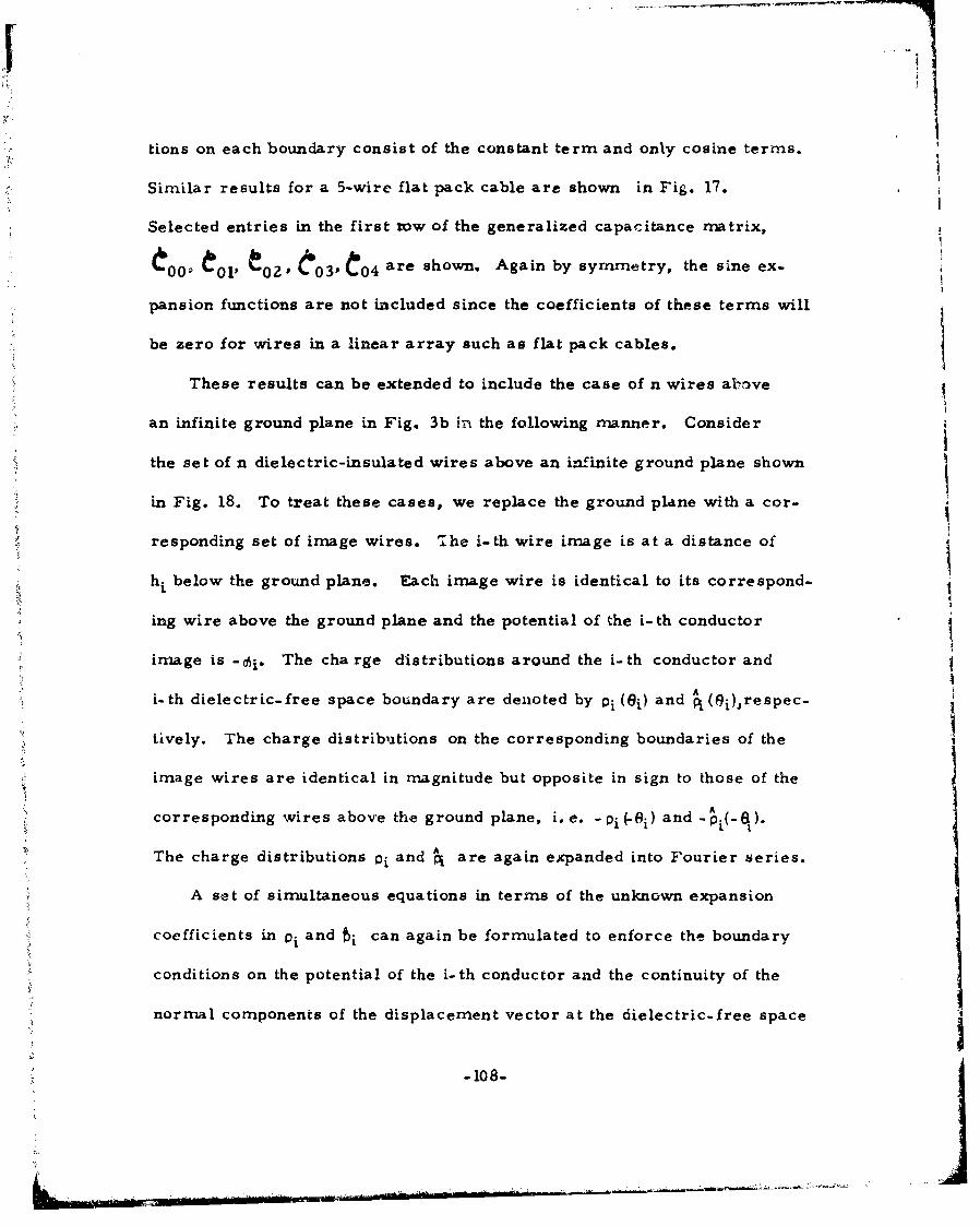
tions on each boundary consist of the constant term and only cosine terms.

Similar results for a 5-wire flat pack cable are shown in Fig. 17.

Selected entries in the first tow of the generalized capacitance matrix,

too0 •0o' •02' t03' o04 are shown. Again by symmetry, the sine ex-

pansion functions are not included since the coefficients of these terms will

be zero for wires in a linear array such as flat pack cables.

These results can be extended to include the case of n wires above

an infinite ground plane in Fig. 3b in the following manner. Consider

the set of n dielectric-insulated wires above an infinite ground plane shown

in Fig. 18. To treat these cases, we replace the ground plane with a cor-

"responding set of image wires. "ihe i-th wire image is at a distance of

hi below the ground plane. Each image wire is identical to its correspond-

ing wire above the ground plane and the potential of the i-th conductor

image is -a0i. The cha rge distributions around the i-th conductor and

Ai-th dielectric-free space boundary are denoted by oi (8i) and pi (ei),respec-

tively. The charge distributions on the corresponding boundaries of the

image wires are identical in magnitude but opposite in sign to those of the

corresponding wires above the ground plane, i.e. -pi(9i) and -Oi(-t)V

The charge distributions 0Land • are again expanded into Fourier series.

A set of simnultaneous equations in terms of the unknown expansion

coefficients in pi and hi can again be formulated to enforce the boundary

conditions on the potential of the i-th conductor and the continuity of the

normal components of the displacement vector at the dielectric-free space

-108-

Er 3.0

t-I1.0

I1

I'/

.5-

.44

S00x-c 00

I • + -c 03-,-C 04

.2-4

SNumber Of Harmonic Expansin Functions

S Per Bowdary

•'Figure 17. Compouted results for a five-wire, ribbon cable.

+ - 109-

.2 7

-0____

hii2 hi

/4 /gr[und

777T71-tlT117I7 o

Figure 18. Dielectric-. insulated wires above a ground plazie and

the image distributions.

_ aI

I °boundaries of each wire due to all charge distributions in the system

(the distributions on the wires and their irnagesl. By symmetry and then A A

use of image distributions,we only need to write ! (2 + Ai+Bi + Ai+B.)i=l I

equations to enforce these boundary conditions on only the original n wires

above the ground plane. Once these equations are solved, the per-unit-A

length transmission line capacitance matrix, C, can be directly obtained

as before since, for this case, oi=vi where Vi are the transmission line

voltages with respect to the ground plane as shown in Fig. 18. Thus for

this case as for Fig. 2b, there is no need to reduce the generalized capa-

citance matrix to the transmission line capacitance matrix via (111).

The per-unit-length transmission Y V inductance matrix, L, can be

obtained accurately by repeating this solution with the insulation dielectrics

removed and using (89ý as indicated in Section 5.1 or using the large-separa-

tion approximation in (122).

The solution for n wires in a circular shield in Fig. 3c can be ob-

tained in the same fashion as discussed in Section 5. 1 for the case of

Fig. 2c.

The above discussion of the solution for C assuming perfect dielec-

trics indicates a method for incorporating dielectric loss and therefore

obtaining an equivalent per-unit-length conductance matrix, G, to repre-

sent these losses. If each dielectric permittivity is considered to be

complex, i.e., ei = e{- iJi - J((di/i.) then (129) can be formulated as

above with the only difference being that P will now be complex. In

- ii

A A

particular, the last I + A. + Bi rows of P will be complex. Thus the nX n

curnplexcapacitance matrix can be obtained as above as Q =9% +JGlso

tha t j, C- = JR" we•and the imaginary part of C can be identified as

= - w CIO The real part, CR, is identified as the usual capacitance ma-.

trix and will of course not be the same as the n-rtrix which would be corn- *1

puted assuming a perfect dielectric.

Large-separation approximations can also be obtained in a fashion

similar to Section 5. 1 by requiring that the separation between all wires

be large enough so that the charge distributions around the dielectric-free

space boundaries and the conductor- Uelectric boundaries are essentially

constant. I-{owever. this is generally not the problem of interest since

wires are closely-coupled in densely-packed cable bundles and flat pack\-1

and ribbon cables and it is to be expected that the charge distributions

around the boundaries will exhibit large variations.

However, to illustrate the application of the technique, the per-unit-

length capacitance between two dielectric-insulated wires which are widely

separated will be derived. Consider the case of two dielectric-insulated

wires shown in Fig. 19. Because of the assumption of large separations,

we may assume that the charge distributions around the conductor-dielec-

tric boundaries and the dielectric-free space boundaries are constant.

Therefore, only four expansion terms are needed in (95) and (128), a 0 0 ,

Aa 0 0 , al 0 , A10 . To facilitate the derivation and provide an upper bound on

the per-unit-length capacitance, we will take the match points at the

.,:, -112-

-- ~--- ---- '

-. - - *c,~ -- 0

-- -0

4 KFigue 1. Atwowir lie ad te slecionof h- atc nonts

-113-

boundaries on a line joining the centers of the wires as shown in Fig. 19.

From the previous results and Table I, one may obtain

0= a 0 0 (ýrw0 'nlrwl) "al0( rwi Ln(d'rw0) (132a)

A A(rw0+to tn ( (rwl + tl) In (d-rw0)"ao0 e v "a1 O ---- v

a ar

rwo tn (d- rwi)___ rwJ (rw 1 )ao0 alo (132b)

ev ev(r0 0 rw +n~ -__t

"(rwo + to)n (d- rwl) A (rw + (r] + t1 ))

Irwo (Cr -1 wlerl)132ao0 CrwO' + to) (alO R (rw0 -. T )A Ao l ~ (rwi + ti) (qr'0 L) 0*4 ao0 i -alO (d-rwO - to) 0

____rw0 (rl- (erl -1) (132d)ao0 ((d-rwl -t 1 ) "alo (rwl + tl) d

+Ts(0 ((drwO +tO)(e.rI'rw t ) + (1) = 0

where CrO = o / Cv and rrl / ev.

These equations may be solved for numerical values of the parameters

as outlined previously. However, in literal notation, the solation is quite

complicated. Therefore, to simplify the solution and obtain a closed forrmi

expression for the per-unit-length capacitance, we will assume that the

wires are identical, i.e.,

-114-

rwo rwl =rw (133a)

to tI t (133b)

C0 = el = C (133c)

Pr = CiCv (133d)

With this assumption we may take the charge distributions on wire 0 to be

identi,'al to the charge distributions on wire I by symmetry. Furthermore,

ql = Zrrrw a10 (134a)

qt

qo Zyraoo0 (134b)

A ,

q 2nr (rw + t) at0 (134c)=q

-ii

40 ZT ( + t) A4O (134d)

Substituting (133) and (134) into 1132) yields II nrw •nr w+t' A

(b r r t(CTr q + In (r Wt) q ~ (135a)

Ji_

" € I - • ¢ '0- q + t ~n W 1 3 b

I Z tT r ( Wc + r(1 F. ) qj (135b)(q,-)) + (er-) ( 'r -1) - 1 ) 4= 0 (135c)

'!i(rw +0) (d- rW- t0 q (d- rw - t) (r w 7+t)

+ ( A+--) ( w -t) -+ q 0. (135d)

\.(d-rw-t) (r t (d- rw -t) (rw +

Note that (135a)and (135b) show that

0 -(136)

and (135 c) and (135d)are identical. Therefore

"V = (1to (0 37)

2 -15-

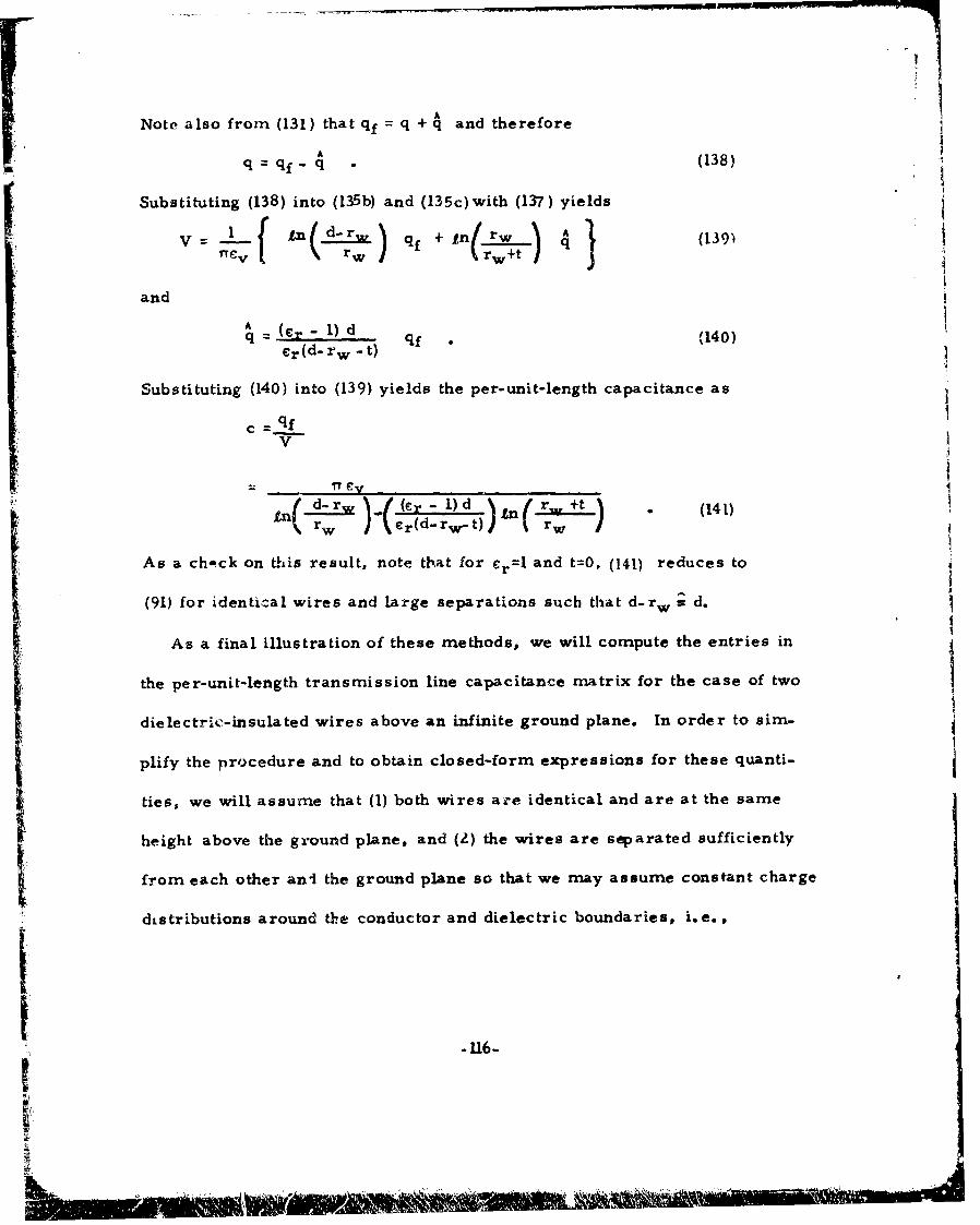
ANote also from (131) that qf =q + qi arnd therefore

A qf.- q (138)

Substituting (138) into (135b) and (13 5c)with (137) yieldsV =i Ln(d-rw.) qf + 1,n(rw )q (1391

ITC tre \ w rw+t

and

A dq (=r - 1) qf (140)Cr (d- rw - t)

Substituting (140) into (139) yields the per-unit-length capacitance as

C =qf-V-

- reyd-rw). .(e'n r)d +t

nd- r" 1cr -wI) d (141)

As a chock on this result, note that for cr=l and t=0, (141) reduces to

(91) for identical wires and large separations such that d-rw w d.

As a final illustration of these methods, we will compute the entries in

the per-unit-length transmission line capacitance matrix for the case of two

dielectrics-insulated wires above an infinite ground plane. In order to sim-

plify the procedure and to obtain closed-form expressions for these quanti-

ties, we will assume that (1) both wires are identical and are at the same

height above the ground plane, and (2) the wires are separated sufficiently

from each other an- the ground plane so that we may assume constant charge

distributions around the conductor and dielectric boundaries, i.e.,

-116-I

q, 2Tr wa 10 (142a)

A A

rdalO (rd rw + t) (142b)

q 2 = 27r rwa 2 0 (142c)

A A

q 2 = 2rda 20 (rd rw + t) (142d)

The ground plane will be replaced by images as shown in Fig. 20. We

A Achoose the match pointsl, t, 2, and 2 on a line joining the two wireg

(other ch.oices are of course possible).

Applying the results of this section and utilizing symmetry we onlyA

need to write constraint equations at i-natch points 1 and 1. The equation for

the potential at 1 becomes (see Table I)

=- v n(rw) q, + in (r) q (143)

+ ln (d-rw)q2 + tn(d-rw)N 2wA

+ In(dl)(.-q 1) + Ln(dl)(-q 1 )

+ tn(d 2 )(-q 2 ) + fn(dz)(-z)qAA

The distances dr, dl, d2 and d2 in Fig. 20 are given by

d,= 4h7+r (144a)dI = 1 4h2 + 2w

d1 =14hZ + rd (144b)

d2 =/40 + (d-r ) (144 c)

d 2 = Ahv+/d-rd2 (144 d)

The equation for the continuity of the normal component of the displace-

ment vector at f becomes (see Table I)

I IA I A

rd r % E. q r q2 (145)

-117-

L *1A" d

4v, 1dlV2

Figure 20. A two-wire line above a ground tdlane and the selectionof the ma~tch pointSo41-

68-2

*~-9 A, -- .- -q2-

q 4.

+ 1 (rd ? ~~ (.+ k ,(d -r ) Ad) 2

"= Cr ('iq ) - C-V.•.. -. •(d q2) A

Collecting terms, (145) can be written a~s

7~) -q 2 )

+ 1 rd A rq 2r) A

(r d.r)drd rd)

/ ~ q 1 e___ ____ (d-rd)A

" (d) + ) + (dr) - ' -) ' 2 0 IS~Since the wires are assumed to be sufficiently separated from each

i other and the ground plane, we may make the following approximations:

Sd1 -•2h

(147a)

i,•. l •'2h({47b)

i : d • h 2 + d 2( 1 4 7 c )

re•

d q

-19

Collctin tems, 145 canbe rittn a

rd r d1 16

d2. dz (147d)

d- r d (14 7e)

d-rd d (147f)*d1

Utiizing these relations in (143) and (146) we obtain (V1 =

2T7O V1 {tfln(• ql + A (148a)

S+ In q2 + An A qz

{ r d I A (148b)

7d d 4

1o-) ((,)z .- ) q2 °

{(Er- d)~ 2 q2 =0 .

The total free charges on the conductors are given by

q =q +q (149a)fl 1 1

f2 = q2 + q2 (149b)

Therefore (148) (along with similar equations at match points 2

A

and 2 ) may be written as

~ [ I LA B [cqiJ + q 3 [ (150)

LVj A Lq 2

C + [A-C) (B-D)]D L q f + jB-D) (A-C)] q2

and.ad] EF] [rqJ + [A n]1 (151)

01 2- G -q2.(11

- 120-

if -

H +

p1

5-,

"C.] qfz [F- (F-H)E- c)

where from (148)

A ILn(4-) (152a)

w

B = In(152b)

C0= In (2h) (152c)

rd

D= B (152d)E dE = ( 1-I) ( 4h 2 Idr (152e)

hdI

F = - ( 1r-) (152f)

r d 1G = ( 1r-l) 4h + r- (152 g)

H =F . (152h)

The variables ql and q 2 can be easily eliminated from equations (150) and

(151) since D=B and H=F and the result is

C~Lqz D (,.-C))f2T~J v ff r--C (A HC G rJIU fJ (153)

Therefore the entries in the inverse of the per-unit-length trans-

mission line capacitance matrix are given by

[C - C (A-C) G (154a)[c-Iu =•r•• C (E-cO

I + rd n .d 1 (( ) rd=•In +-d rd r+ rd- 1C 4

S• e, ÷( )rd I I

Sri. r

for i, j=l, 2 and d' is given by

d 14h+ dZ (155)

For this case, we assumed that (1) the two wires are identical,

(2) they are at the same height above the ground plane and (3) the wires

are sufficiently separated from each other and the ground plane such that

the assumption of constant charge distribution is valid. When these assump-

tions are no longer valid, the expression for the entries in C"i or Q cannot

be easily obtained in closed form and a digital computer must be used.

The expressions in (154) for the entries in C- 1 will be used in a later

publication in the analysis of certain experimental data for which this

approximation is reasonably accurate. It should be noted that an approx-

imantion for c1 2 for this specific example has been obtained in [33] although

the derivation is not presented and evidently relies on certain empirical

data.

im

" ~- 122-

VI. SUMMARY

A complete and unified discussion of multiconductur transmission line

theory has been presented. The general solution of the problem under the

assumption of TEM mode propagation in the case of a homogeneous medium

or quasi - TEM mode propagation in the case of an inhomogeneous medium

has been presented along with parameter derivations and lumped-c;_rcuit

approximations. If losses can be neglected, then it appears to be as efficient

to solve the transmission line equations directly and incorporate the terrnina-

tion networks through the solution of (70), (75) or (76) as it is to use lumped-

circuit iterative approximations described in Section 4. 1. The matrix chain

parameters for the distributed-parameter approach can be easily obtained in

closed form suitable for numerical computation so that "abruptly" nonuniform

lines can be handled and the per-unit-length parameters must be obtained for

either the distributed-parameter or the lumped-circuit iterative approach.

When solving the transmission line equations directly, one is not required to

solve an increasingly-large (although sparse) set of equations for increasing

frequencies when the line is not electrically short as is required with the

lumped-circuit iterative approxim& rions. For ýhe homogeneous-medium case,

a lossy dielectric can also be included with no additional computational dif-

ficulties. Lossy conductors will also present no additional computational

problems for the homogeneous-medium case if tht n conductors are assumed

to be identical. When losses cannot be neglected in the case of an inhomo-

geneous medium, the question becomes more difficult to answer since

-123-

i diagonalization of YZ, whi(h is roequired in a direct solution of the. trans- jmission line equations, is, in general, required to be performed at each

frequency and is not necessarily guaranteed except in the case of cyclic

symmetry matrices which assume certain structural symmetries of the

line as described in Section 3. 3. For this case, it may be preferable to use

one of the lumped-circuit iterative models for frequencies where the line is

electrically short, e.g., X< 10 X and approximate the line with only one10

section, i.e., solve (80) with N=l. For frequencies such that £> / 0 ,x it

may be preferable to solve the transmission line equations directly rather .

than increasing the number of lumped-circuit sections to approximate the

line since no quantitative criterion for determining the required number of

sections for a given approximation accuracy can evidently be obtained.

Numerical techniques for obtaining the per-unit-length parameters for

bundles of closely-coupleddielectric- coated wires as well as large-

separation approximations for wires in a homogeneous medium are also

given.

-124- A

RLI

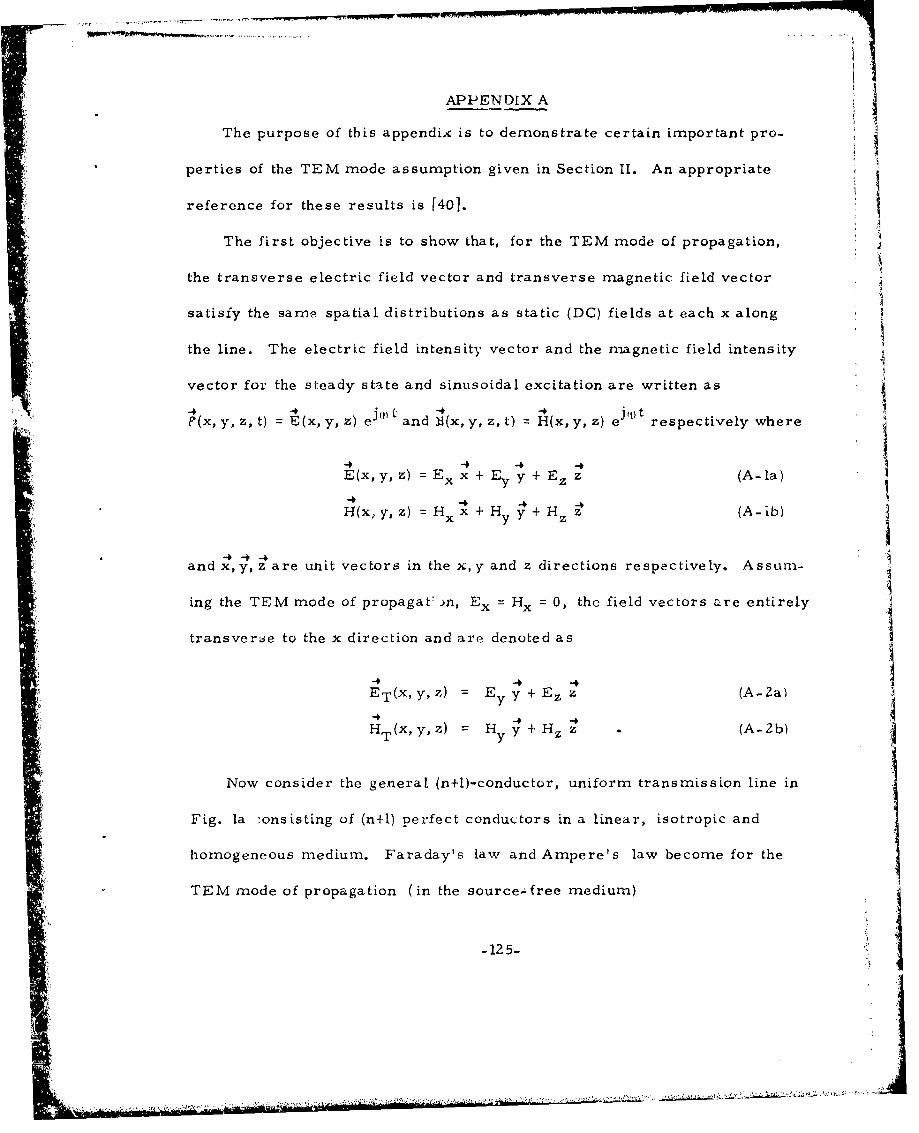
APPENDIX A

The purpose of this appendix is to demonstrate certain important pro-

perties of the TEM mode assumption given in Section II. An appropriate

reference for these results is [40].

The first objective is to show that, for the TEM mode of propagation,

the transverse electric field vector and transverse magnetic field vector A

satisfy the same spatial distributions as static (DC) fields at each x along

the line. The electric field intensity vector and the magnetic field intensity

vector for the steady state and sinusoidal excitation are written as

('(x, y, z, t) = E(x, y, z) e and JI(x,y,z, t) = H(x,y, z) respectively where

E(x,y,z) = E x + Ey y + EZ z (A-la)

._•:J{ (x, y, Z) = H x• + H y y + Hz z• (A- 1b)

and x,y,z are unit vectors in the x,y and z directions respectively. Assum-

ing the TEM mode of propagat'• n, Ex = Hx = 0, the field vectors are entirely

transverse to the x direction and are denoted as

ET(x,y,z) = Ey y + Ez z (A-2a)

HT(x,y,z) = Hy y + Hz (A 2b)

Now consider the general (n+l)-conductor, uniform transmission line in

Fig. la "onsisting of (n+l) perfect conductors in a linear, isotropic and

homogeneous medium. Faraday's law and Ampere's law become for the

TEM mode of propagation (in the source-free medium)

-125-.

.~~~~~ .~~- .- .

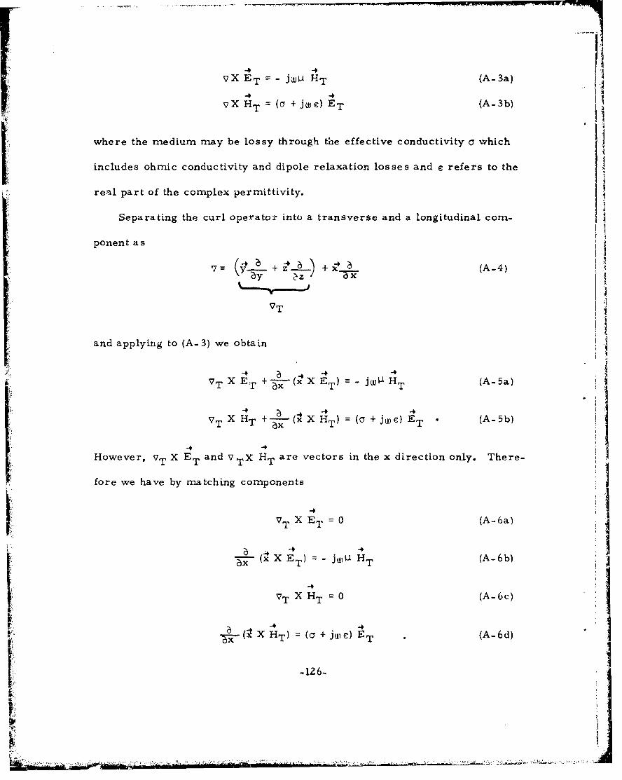
"4 "4

vX ET = - .HVk NT (A-3a)

vX HT= (a + juve) E(AT3b)

where the medium may be lossy through the effective conductivity a which

includes ohmic conductivity and dipole relaxation losses and e refers to the

real part of the complex permittivity.

Separating the curl operator into a transverse and a longitudinal corm-

ponent as

"7= + 2S" + Xz (A4

VT H

and applying to (A-3) we obtain

4 44

T XrE +T )X +T( = - jUj HT (A-5a)

"4 4 4 4

VT X HT +-(x X HT) =(a +jue) ET • (A-5b)

However, VT X ET and VTX HT are vectors in the x direction only. There-

fore we have by matching components jLii

• 41T X ET (A-6a)

(x€ X ET)= jau" HT (A-6b)

T XHT =0 (A-6c)

a 4 40 X HT) = (a + ju)C) ET (A-6d)

-126-

I

I I

Note also from V.D= p and V.B= 0 so that

,VETVT.ET = (A-7a)

-4 4 #v- HT VT.HT 0 (A-7b)

(since Ex = H= 0) where p is the free-charge density in the surrounding

medium (which will decay to zero with time cons#-ant c/l). Therefore,

equations (A-6a), (A-6c), (A-7a) and (A-7b) show that the transverse field

vectors ET and HT satisfy the same spatial distributions as static fields in

any transverse plane (y, z) at each x along the line. 4

This may be more easily seen if we write Faraday's law and Ampere's

law in integral form by applying Stokes' theorem to V XE = - jjIH and

44

SVXH =r (+ j(#)e) E + as

E Ui jwi H" da (A-8a)

gH dt= ea +. (a+ jwj ) E. d~ (A-8b).S S

where C is a closed contour enclosing the open surface S. Taking C to be a

contour in the transverse (y, z) plane denoted by Cyz and S to be a flat

surface in the transverse plane denoted by Sgz which is bounded by Cyz then

(A-8) beccmes

S(Ey dy + Ez dz + Ex dx) =j,,, Hx dy dz (A-9a)G-yz Syz

S(H dy+ Hz dz +Hx dx) Jx dydz +(a + We Ex dydz(A-9b)"C Cy Syz syz

1_ -127-

?I .

v.here Jx is any source current in the x direction penetratiT.2 , HS-'e'.et,

unde" the TEM mode assumption E. = Hx = 0 and (A-9) becorues i

d + Ez z) = ET " (•d z + -4 dy) 0 -taS (E d ~E dz)= ET(d dy= (f\- Lea)

cyz cvz

(H d y+ Hz dz) ~ HT (dz + yd 5)S x~~l? AldCyz Cyz Syz

4 4which are of course indicates that E.,. and HT are no longer coupled iogolter

::s is the case for static electromagnetic fields.

Thus we may uniquely define the voltage of the i.-th conductor ant' i'.,

.irrent associated with the i-th conductor as

Vi(x) = Ci ET di (A-II)

Ai(X) HC^ T •di, iA, - I L)

A',.here C. and C. are shown in Fig. lb as contours in the transvo'rse M,'n,,

u. particular x along the line.

The second objective is to demonstrate that for (r+!) perfect cond~U,.

" r.. . n' ou, mledil.,lr , t, ' r- uni te :- i,, ", ".' : . '',, .

i. .l y the important relatjun- T il .4". , : "v'. ' - t',,

-* r, y oltai_ by takinng the p,3ar t, d r, ,,v i - c ' . .. IY and taking the curl of x with each equation.

iI' '

't . .

SHT = (jw - I2 uie) HT (A-12a)

- Tw2 ET =- ue)ET (A-lb)

From equation (19) assuming perfect conductors

dx2 Y Z I(x) = (jwGL- (12 CL) 1(x) (A-13a)

dX(x) = Z Y V(x) (j., wLG - w2,LC) V(x) (A-13b)

Performing the operations indicated in (A-Il) on (A-12) one obtains two sets

of n equations

d2I.d"-& Ii (x) = (juoUa" vu¢ i (A-14a)

d----VL I X) =(j W Lr _ W2 U C) Vlx) (A-14b)

Arranging these fo(r i 1, - n as in (A-13) shows, by matching real and

imaginary parts, that

LG = G L = u a (A-15a)

LC =C L = uc (A-15b)

-12 9-

il -ail-

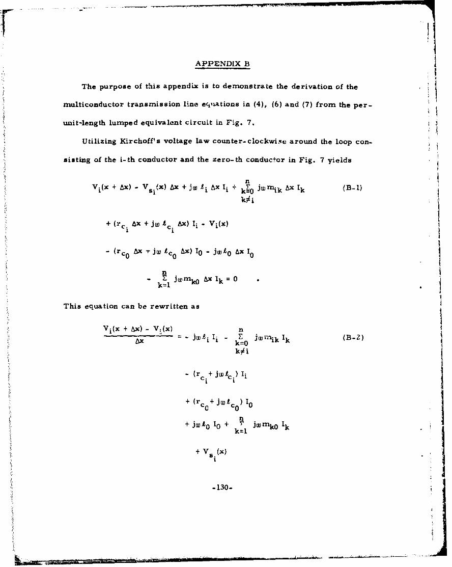
APPENDIX B

The purpose of this appendix is to demonstrate the derivation of the

multiconductor transmission line equations in (4), (6) and (7) from the per-

unit-length lumped equivalent circuit in Fig. 7.

Utilizing Kirchoff's voltage law counter-clockwise around the loop con-

sisting of the i-th conductor and the zero-th conductor in Fig. 7 yields

nVi(x + &x) - Vi/x) &x +j(" i t'x I + kro jWrnikA Ik (B-I)

k~i

+ (rc x +jW I Ax) I - Vi(x)

- (rco 6x iwj 0 t1x) 10- jL 0 Ax 10

n

-~k &x jmxIk 0-k=1S tm0 • i =

This equation can be rewritten as

Vi(x + Wx) - V-lx) n•.• =-jW~i Ii E jrnaik 'k (B-2)Ax k=0 (

k# i

(r+ JW•c) Ii

+ (rc+ jWt I

C0n

+ jW10 10 + 5 jWmkO Ikk=1

"+V (x) I-130-

L.

and the current in the reference conductor satisfies

nI0 r I k (B-3)

k=l

Substituting (B-3) into (B-2) one obtains

Vi(x + 6x) - Vi(x) (B. 4)

&x " i Ii . Jw(-rnio -I -n 1 0 In + Iron LI+''" +rmin In)

- (rci + jigii ) I.

+ (rc + J (1, i + J (vto)Co 0I ... n)

+ j w(m1 0 I +.... + mno In )

+ Vsi(x)

which may be rewritten as

Vi(x + Ax) - Vi(x)- - (rc 0 + jW'c 0 + j -o jwm(0 " Jwmio + jwomil) I1 (B-5)

S.... (rc. + jnif + jwLti + r + jWUc +jWL 0t

jum - jWmi0) -i ....

.. (rc 0 + jWIL, + jW1.0 - jWnn0 - Jwmi + jWm

+ Vs. (x)1.

Arranging these equations for i=l,---,n and taking the limit as Lx -. 0 yields

(4a)and the per-unit-length impedance matrix, Z, can be separated as in

-131-

I~iin~mm

(6a) with the entries given in (7a), (7b). (7c).

The derivation of the second transmission line equation, (4b), proceeds

similarly. Utilizing Kirchoff's current law for the i-th conductor in Fig. 7,

we may write1

11(x + Ax) = li(x) - (gi x + jwci0 Ax) Vi(x + Ax) (B-6)

nE {gik Ax + jw•ik Ax)(Vi(x + Ax) - Vk(x + Ax))k=l

k i

+ Isix) W x

which may be rewritten as

Ii(x + 6N) - i(x)

&x = (gil + jWC i) VI (x + Ax) (B-71

+ ... (gio + jwcio + k=1 (gk + jwcik)) Vi(x + &x)

k i

+ + (gin + Jwcin) Vn (x + Ax) + s i (x) .

Arranging for i=l,---n and taking the limit as Ax 4 0 yields (4b) and the

per-unit-length admittance matrix, Y, can be separated as in (6b) with the

entries given in (7d) and (7e).

-132-

4

t' , . •......,• ',o.,-.•.'., -•.,, . .. , r ,:•••.-"- """0 •'••''•'a:'-' •'-'••'

• I

APPENDIX C

The purpose of this appendix is to derive the expressions for the per-

unit-length equivalent sources in (5) which are induced by an incident elec-

tromagnetic field on the uniform transmission line in Fig. 2a consisting of

(n+l) perfect conductors in a lossless, homogeneous meuium (see Fig. C-I).

The expression for the currents induced in termination networks given in

(77) will also be obtained. The solution for Fig. 2b is also discussed.

The solution for the special case of a two-conductor line (n=l) was

obtained by Taylor, Satterwhite and Harrison in rZO] and later in a more

convenient form by Smith in r2i]. The solution for the case of a uniform

plane wave incident on a three-conductor line in the transverse direction

(perpendicular to the system's longitudinal (x) axis) with the electric field

intensity vector polarized parallel to the line axis was obtained in [24].

Procedures for extending this result to multiconductor lines were indicated.

It is convenient to consider the effects of the spectral components of

the incident field as per-unit-length distributed sources along the line [26].

The sources appear as series voltage sources and shunt current sources as

indicated in Fig. C-a for an "electrically small" 6x section of the line. The

multiconductor transmission line equations may then be derived for the

&.x subsection and are given in equation (4). The termination networks are

given in the form of generalized Thevenin equivalents as in equation (69) and

the solution for the termination currents is given in equation (75). Substitu-

ting the expressions for the matrix chain parameters given in (49) into (75)

for this case of

-133-Kr

rr

I

W I_ ri , ¶-

E,1

d if(X) I In Vi(X+ A~X)

4 I

SAx X+Ax

Figure C-i. A multiconductor line with incident field illumination.

-134-

L,

________________________________________________ II 1

r+

+ ++ +

On

K _ _ _ _ _

K0

-< x

K E

#A _

Figure C-2. The Der-himit-length equivalent, circuit for Fig. C-1.I' -135-

perfect conductors in a lossless. homogeneous medium (free space)

described by e and Li , we obtain

rcsoIfz+ z + j ssin(e~ {Z1a 1 c ()(-~)

0 -1 4 + coz( Z) 'Zn] 1r (0

- + [J sin(O PZ ze + c o(B)nJV0

A A+ - z1(•)

I!(Mr) = -j )z + rcos(1) I + j s9W(01) ZcZ 1o](0 ) (C-lb)

where the wave number is ; = Zrr/X, X = u/f. u = 1/411 -c, 3 x 108 m/sec.

The characteristic-impedance matrix ZC becomes

Zc uL (c-2)

AA

and V,(S!) and [a(Z) are obtained by substitutLng (49) into (74) as

V W '{cos(B(Z-,A)) V () - j sin(o-)) (I ()} dXla (C-3a)

AA-1 A A\ cos(O (.C- A)) I - j sin(8 (Z- x)) Z V x (C-3b)0

Solution of (C-la) for the termination current vector, 1(0), requires the

solution of n complex equations in n unknowns (1i(0)). Once (C-la) is solved,

(C-lb) yields the termination currents.I(Z) directly.

Although the equations may appear formidable, they are in a compact

form and can be straightforwardly programmed on a digital computer.

-136-

Furthermore, the form is not restricted to any particular value of n. The

A Aonly difficulties are in determining L and determining .Vs and I1 (which

require that we determine Vs(x) and I (x)). The determination of the equiva-

lent sources Vsi(x) and Ii(x) induced by the incident field will be the next

objective.

C. 1. Def:ermining the Equivalent Induced Sources

In order to determine the equivalent induced sources, Vs (x) and Is (x),L I

consider Figure C-1. The method used in [2zo can be adapted here in a

similar fashion. Faraday's law in integral form becomes

E de jwLv H • ida (C-4).. Si

where S. is a flat, rectangular surface in the x,y plane between wire i andL4

wire 0 and between x and A + &x as shown in Figure C-I. The unit normal n

is n z where z is the unit vector in the z direction, da = dx dy and C. is a

contour encircling Si in the proper direction (counter-clockwise according to

the right-hand rule). Equation (C-4) becomes for the indicated integration

di[Et.(y, x+x) - Et(y, x)Idy (C- 5)

0 1x+Ax

[E.(dx)- EL (O,x)]dx

X+6x dio

S"x 0 11. In integrating from y=O to y:-dio, we are implicity assuming that rwi and

r"o are much less than dio, i.e., the wires are sufficiently separated so

that they may be replaced by filaments.

-137-

where Et. is the component of the total electric field (incident plus scattered)

transverse to the line axis and lying along a straight line joining the two

conductors, i.e., E4* Ey; E is the component of the total electric fieldLt y' I

along the longitudinal axis of the line, i.e., .7 E x aid Hni ia the com-

ponent of the total magnetic field perpendicular to the plane formed by ithe

two wires, i.e., Hn. = Hz.

Defining the voltage between the two wires as

Vi(x) - Et (yx)dy (,C-6)0 ,i

then

P ~dVi(x) I •ao= -I'V1 L)ý Ft (y, x+x) - Et (y, x)]dy (C- 7)

dx x-irn 0 0 t.

The total electric field along the wire surfaces is zero since we assume

perfect conductors. (One can straightforwardl]y include finite conductivity

conductors through a surface impedance as w-as done in f201). Therefore

(C.-5) becomes in the limit as Ax4 0

dVi(x) •dio

dx J- v "0 Hni (y, x) dy (C-8)

The total magnetic field is the surn of an incident and a scattered field:

Hni, Hz (y, x) (C- 9)

(rca t) (inc): 1 HZ(Y, x) + H Z (y " x)

scattered incident

-133- i

and the scattered field here is produced by the transmiseion line currents.

The scattered flux passing between the two conductors per unit of line lent

is directly related to the scattered magnetic field and the per-unit-length

inductance matrix, L, as

(scat) d (scat)1.x) = " dv Hnj(Y' x)dySti o

H~f (yxld

II(x)12 W

In(X)

where i= L]j" Substituting (C-10) and (C-9) into (C-8) and arranging for

S -----, n yields

.d (inc)

(x) +LI(x) Hn(y, x)dy (C- I)* 0

and the source vector V (x) in (4) is easily identified by comparing (4a) and

?;• (0-11).

d For transmission line theory to apply, the cross-sectional dimensions

of the line (wire spv cing, etc.) must be electrically small, i.e., dio << 1

and dj << 1. Thus the result indicates that the voltage, Vsi, induced in

the loop between the i-th conductor and the zero-th conductor and bet'ween x

and x+Ax is equal to the rate of change of the incident flux penetrating this

"I"electrically small" loop which, of course, makes sense.

"•:" ~-1-39-

npe-'e's law yields

E j (C-l1Z)y=- wex z a]

E will consist of scattered and incident field components and is written as

Et.(Y. X= Ey(Y. x) (C-13)

(scat) (inc)

=E (yx) + E, (y.x)

scattcred incident

il iSubstituting (C-12) into (C-6) we have

(scat) (inc)doI dio f a Hz(y, x) a Hz(y, x) .

V. (X) E (Ey, x) dy = j+(C- 14)

1 0 v jw O(scat) (inc)

- Hx(y, x) b Hx(y, x)

Utilizing (C-10) we obtain

d 11(x))

jw e c ill i2 dio (inc ()G

ii If we assume that the currents on the wires are directed only in the x

",direction i. e., (there are no transverse components of the currents on theI

dl (scat)

wire surfaces), then Hx(y,x) = 0 and (C-15) becomes

je - 14 O-

v 0 t

d.d

-- dio (inc)C0' Et(yx)dy

Arranging these equations for i = 1, --- , n we obtain the second transmission

line equation

I d 0 " (inc)

i(x) + jwev L 1 V(x) = e L- x)dy (C- 17)V0 :

Utilizing the important relation for a homogeneous medium, C = 4vev L-IL in

(C-17) we obtain by comparing (C-11) and (C-17) to (4)

d (inc)

(s = W . Hni(y, x)dy (C- 18a)v0 .

L •

iis (x) =- juu C Et. (y. x) dy ( C- 18b)S0 • 0

I "

The shunt current sources in I S(x) are therefore a result of the line voltage

iI induced by the incident electric field being applied across the per-unit-lengthil ~line-to-line capacitances which, of course, satisfies our intuition.

[ .~141 -

-. . . . .. . . . .. . .. .. .. ....... .... . .. . .-

A A

C.2. Solution for V (x) and I (x)

The final problem remaining is to obtain simplified versions of V and

AI in (C-3) to be directly used in (C-I). First consider the determination of

AV5 (1). Substituting (C-18) into (C-3a) yields

A d. * ý(c)0s 1 " 0 0

i£ -d 0 .(inc) A A

S- sin((- x) E (YX)dYy dx0 0 *L j

From Faraday's law we obtain

(inc) (inc)(inc) 1 aEIi rEti

=---- -Wv y; (C- ZO)

Substituting this into (C-19) yields

A (inc) (inc)V = fcos((£-_) A)) - ELi (0,f CIA (C-21)LI

0 ax

6 .

{cos( (£- x)) y-d2

I.• 142-

B-+

- ~~ (inc)A 1fs i (.CX"))Et. (Y.x) dy d

0*0

Utilizing Leibnitz's rule,(C-Zl1) is equivalent to

A 4A (inc) (illc)

S(eo s(~) E; (di E E(OAc) }.4 (C- 22)

- 'a fCSO ) d. (inc) d

ox x t(. d I

and this m-ay be written as

A er A (inc) *(inc)A

-s (.)= fcosB x)) E (d10 & - EL (0,X) d.c (C-23)

d.o (inc) ýdio (mc)

-t E(y,9) dy + cos(OX) \ Et.(y, o) dy

-143-

SimilarilyIs (£l may be obtained as

-(inc) .(mnc)

_f-i( (i- x)) Eti(dio, x) - . l (C-24)

1'.o (mnc)3-z L~ in Z1) E~ (y,O0) dy

0. i

A AThe important quantity in (C- la) is V ( Z Combining (C-23)iand (C-24), thia becomes

V(1) - X ~~ f~o((4 )) I + j sin((S-c)Z 1 (C-.2 5)

F •

X z Z-8 0 n(m) n•.) 0 zc

Ir

(ic.(ic, A Ado (icThe Irprat qu(dtity X in (C- X) isVa(£ .0 t£i(y,• Zo)iin (C2

- 144-

vn C 24,ti btne

0 ti•dio ic

+[cos¢•£1n +j sin( Z) Z£ Z (y, ( )nc)

Note that the equivalent forcing function on the righthand side of (C-la),A A

V.(Z) - Z I.(), given in (C-25) is simply determined as a convolution of

differences of the incident electric field vector along the wire axes,Oinc) (inc)

Efi(dio,x) - Ei(Ox), and a Fnear combination of integrals of components of

the electric field vectors at the endpoints of the line which are transverse to(inc) (inc)

the line, Eti(y.Z) and Eti(yO). This is, of course, precisely the result

obtained by Smith [Z1] for two conductor lines. Substituting (C-25) into (C-la)

and settingV n= V0 V = 0 , i.e., no independent sources in the termina-n-1 n-l

tion-networks, one can verify that the result reduces for two-conductor lines

(n=l) to the result given by Smith [21] since ZC, Z , Z become scalars for

two-conductor lines and (C-la) becomes one equation in only one unknown

1(0). Por uniform plane wave illumination of the line (which is usually the

case of interest), (C-25) reduces to a much simpler form although the result

allows for the more general case.

The final equations for the line currents then become (substituting (C-25)

into (C- 1))

rsZ)z+ ZZr +j s in($ ) Z +Z ZZ Z };Z 1 (0) (C-26a)

-145-

V,

10_ C

- v•+ rjsn(s•) z• Zc- + cos(B•)1!]VX

(inc) (inc)- ~IZ)+ {rco0 (O) 1 + jsin(B 1) Z cJ.t(0)}

L(Z) j- s in(Z) ZC' V 4 [cos(.Z) lI +j sin(P.Z) Z Z 0)I(0) (C-Z6b)

I (inc)-jZ

1 s {in (5(Z-) Eji) }dxc

(inc)- szi- {si• ),( _E (O)}

( i oc ) ( o c ) ( o c )where EI (x), .Et(Z) and E t(0) are n y I column vectors with the entries in the ii-th rows given by

(inc) (inc) (inc) "-ýE •z (X)]= E• (d i0,X) - E 1. (0, X) (C-26c)

(inc) dio (inc)[Et(a)]i=. Et (9i,£ ) dt, (C-26d)

"0

LEt(0)]i E• Et. 0,) dý i (C-26e)

for i = 1, ---- , n which are equations(77).

A word of caution in the interpretation of the notation is in order.

Although it should be clear from the derivation, the reader should neverthe-

(inc)less be reminded that the integration path for the component Et is in the yi

direction when the i-th conductor is concerned. When other conductors areii concerned, the integration path is a straight line in the y, z plane which

-146-

•:.

-.... .'

joins the conductor and the zero-th conductor and is perpendicular to these

two conductors. This is designated as ýi in (C-26) and replaces the y vari-

able for the path associated with conductors i and 0. The notation may be

cumbersome but the idea and implementation is quite simple.

C. 3. The Per-Unit-Length Inductance Matrix, L

One final calculation remains; the determination of the per-unit-length

inductance matrix, L. Ordinarily this is a difficult calculation as discussed

in Section V. However, if we assume that the conductors are separated

sufficiently such that the charge distribution around the periphery of each

4' conductor is constant, then the conductors can be replaced by filamentary

lines of charge. Typically, this will be quite accurate if the smallest ratio

of conductor separation to wire radius is greater than 5 r56]. In this case,

the entries in L are shown in Section V to be

= - 2n ( ) (C-27a)

vu vv' i 7 (r rdrw two

;'• For closer conductor spacings, proximity effect will alter the charge distri-

,• butions from constant onaes and numerical appreoximations must be employed

to find L as was discussed in Section V.

The entries in the per-unit-length inductance matrix

for large wire spacing given in (C-27) can be derived in an alternate manner

-147-

wp PIW•

.,1

which more clearly illustrates its relation to the total scattered flux passing

(scat)between the wires. The matrix L relates the scattered flux 0 passing

between the wires to the wire currents as

'.(seat)-...el II"" ln Il

(scat)- . - .. . (C-28)

(scat)On .Lnl" . . . n

The respective entries are determined as

(scat)

Ii Iil, I i+I. In 0 (C-29a)

(scat)

and Ii =ji" Large wire separations are assumed so that the wires may be

replaced by filaments of current.

Consider Fig. C-3a. The magnitude of the magnetic field intensity

vector due to Ii on wire i at a distance r > rwi away from wire i isII

H = -- (C-30)r 2rrr

and the total flux passing between wire i and wire 0 due to both currents is

-148-

!I•

Hir iIjI

(a)

IIjGd

dddj

H-H

(b)

Figure C-3. The oroblem geometry for the calculation of the entriesin the oer-wnit-length inductance matrix.

-149-

(scat) fdio I drdr + dr (C-31)

r wir

2rI rwi nwo

Thus L.. is easily identified as in (C-27a). fIL

(scat)Consider Fig. C-3b. The portion of the flux passing between

wire i and wire 0 due to -I in the reference conductor is as above

(scat) uv~i (Oi0 =n (C- 32)

and the portion of the flux passing between wire i and wire 0 due to I. in the

j-th conductor can be found to be

(scat) = diod -~~ (P - PO)(C3

i-. Combining (C-32) and (C-33) we obtain

bI

Comsince

snd.. =i 0 + (d - 001P (C-35a)

-ISO--150-

E)I

do02 = to+ p (C-35b)

and zij is easily identified as given in (C-27b).

C.4. Computed Results

To show the simplicity of the result and indicate its equivalence to the

result obtained by Harrison in [241, Example I considered in [7_141 will be

computed by this method. Three wires all of radius 10"3m lie in the x, -

plane as shown in Figure C-4. A uniform plane wave with an electric field

intensity magnitude of IV/m is propagating in the y direction and 500Dl

(purely resistive) loads connect each line to common nodes. The various

distances in Figure C-1 are d10 10 m, d2 0 = 2 x 10-2 m and d12 10 M.

and Z can be easily shown to be

- 1000 500¾7d= z° = 0° O

The characteristic-impedance matrix, using the values for the per-unit-

length inductance matrix given in (C-27), becomes*1in(lOO) Ln(20)

Z =uL 60, [n(20) �n(4 00)

i (inc)

Et = 0 in (C-26) and the electric field intensity of the wave is

(inc)E (y.x) = E -joY

£ x

}.: - 151-

50041 5004___ __

V2(O))

50092 Ijý(O) 500iL

50O0n)+()~ ,O 10-2 m 500PQ

Uniform Plane ~ 3

Wave Propagating/Z in +- y Direction

ExzI V/rn jy

Figure C-4. The geometry for the example.

-15 2-

From this, one can determine

(inc) (inc) B1 -EN (d 0 ,x) - EL (0,x) = e"810 -1

(inc) (inc) -j210-2EY2 (dz0, x)- EL(0,x) e-1-

Two frequencies are considered in [24] in terms of x; 1-- 1.5, Z 3.0.

Equations (C-26) with the above items were programmed on an IBM 370/165

computer in double precision arithmetic. The execution time (cpu time)

was .01 seconds (1/100 sec) and the results are

"JIo(O)I= 1.7662556E - 5A /I0(0) 70.770

0.- 1.5 lIl(0)j = 9.0756083E - 8A /I.(0) = -13.9o{I2(0)1= 1.7671218E - 5A /I(0) =-109.520

110(0)I= 5.4543875E - 5A = 9.8450

OS= 3.0 11 (0)I = 7.7363155E - 7A 11(0) = -75.80

S111I 201 5.4608110E -5A /I()= -170. 96o

The computed results obtained by Harrison' method and given in r 24] are

if(0 1. 766E -5A

0,£= 1.5 1i (0)I =9.076E- 8A

11 2(0)I = 1. 767E - 5A

-153-

JIIIf0(0)l : 5.454E- 5A

e£- 3.0 11 (0)I= 7.7.36E - 7A

]12(o)1 = 5. 461E -A 2IThe results computed by this method are exacti? those computed by

Harrison's method in [24]. However, with this method only 2 simultaneous

equations in the 2 unknowns, 11(0) and I1(0), are required to be solved

(1 (0) -1i(0) - 1 (0)). Harrison's method required the solution of 10 simul-

taneous equations in 10 unknowns. Furthermore, Harrison's method was

restricted to uniform plane wave illumination of the line with the wave inci-

dent perpendicular to the line. Since Z Z 0 for this example and since theI

uniform plane wave is propagating broadside to the line, 1(0) = I(Z).

C-5. Extension of the Method to Wires Above a Ground Plane.

Consider the system of n wires in free space above an infinite

ground plane shown in Fig. 2(b). The result for (n+l) wires given in (C-26)

can be extended to this case with the following observations. Consider Fig.

C-5. Clearly we may apply Faraday's law in (C-4) and the previous devel-

opment to the flat, recfangular surface in the x,y plane shown in Fig. C-5b

between the ground plane and the i-th wire and between x and x+&x. This

flat, rectangular surface Si lies in the x, y plane. Equations (C-26a) and

(C-26b) will again be obtained. Equations (C-Z6c), (C-26d) and (C-26e) be-

"come for this case

(inc (inc) (inc)[Ee(x) i = E ,. (hix) - E9 . (0,x) (C- 36a)

-154-

'-- -- - . . .14g

-* ... .. . -,.. , •~I~ E i I EI IF!B -4inc)t tj

zS7 / /L /, / / / "ground

hiplne

(a)LII

yzh

yVhi ( ) )

/ / / I / /Io., Ij+Ax

plane

I I II Ii I I

,%I / ,

(b)

Figure C- 5. Multiconductor lines above a ground Dlane.

-155-

"L-:-- ••,v "tM- ''' -- ': " -''- 5•1 !••''•-- " •" ° •~ - - -"--•

[ (inc) hi (Inc)[Et M)i = Eti i,) dti (C- 36b)

S(inc). (hi (Inc)[Et ()]i \ Et, (ti, 0 ) dti (C-36c)(0c) \0I(c)3c

where %is a straight-line contour in the x, y plane between the position

of the ground plane, y=O, and the i..th wire which is perpendicular to the Vground plane, i.e. ti =y. This is indicated in Fig. C-5a.

(Inc)E P'. (hi, x) is the component of the incident electric field parallel

(Inc)to the axis of the i-th wire at y=hi and Eti (0,x) is the component of the

incident field parallel to the ground plane directly beneath the i-th wire.

Et. is the component of the incident electric field parallel to gi andEti

directed in the +y direction.

The per-unit-length inductance matrix, L, can be obtained in a

fashion similar to Section C. 3 by determining the scattered magnetic flux

passing through the surface Si between the i-th wire and the position of the

ground plane--(the ground plane is replaced by image wires) and is given

in (122) as .sS-Uv ,,n .2hi], (C- 37a)

[L v in dij(C-37b)

for i, j=l, --- , n where

d I._~+ 4h.h. (-38)ii j i IiL

-156-

[,I

__ _/

-"----- - --- --nn .. . .....

APPENDIX D

The purpose of this appendix is to derive the simplified form of the

nodal-admittance matrix for the lumped-circuit iterative approximations

given in (80) and the forms of the matrix chain parameters given in (78).

To derive the first equation in (80) consider the equations for the termin-

ation-networks in (69):

v(0) V_0 - Zo_1( 0 ) (D-la)

v() z• + Zz• I. (D- !b)

and the matrix chain parameter equations for the lumped-circuit iterative

models given in (79) for a line of N sections:

V (k£) = V (LL Z) + -- 1 I (-L£) (D-ka)

-) = t) D-?.b)-N~z N-Z (Dc2

For the first subsection rewrite (D-la) as

1(0) = Y V - Y 0 v(o) (D-3)

whe.ie YO = •0 and substitute into (D-2a) with k=l to yield

V(/ IN) !•kl V(O) + !kI2. (Yo -10 - Y0 V(O)) (D-4)

= (k4 - !kIZ o0 ) V(o) + U1 -YoJXO

which is the first equation in (80).

••. - 157-

To derive the last equation in (80), rewrite (D-lb) as

_ = :_(X).y Y (D- 5)

Niiwhere Y£ z Z•I Substitute this into (D-2b) for k =N to obtain 1

Y(Z- Y Y:, & I (- + !k2 I) (D-6)

Substitute (D-2a) for k = N into (D-6) to obtain

(D-7)Y£V(£, .v _V1 = I/j~ V(-Nl + V({1 ) -1 •N2 I- +l- I V , II

which can be rewritten as

&.21 -JZ - kZ 41 kZZ N &i I= -ZY~~ D8

However, one can easily prove the identity in (8 Z

i- L21 !k2 -'l2 kll k12(D- 9)

associated with the forms of the lumped iterative matrix chain parameters

in (78). Therefore, substituting (D-9) into (D-8) and multiplying on the left

by "tk2 yields the last equation in (80).

The derivation of the intermediate equations proceeds similarly.

Substituting (D- Zb) for k=m into (D-2a) for k=m+l yields

(MI

Nkll +-kl2{ -012+ N + k22 ( ) D

Writing (D-2a) for k=m as

-158-

•of

(D-1l

and substituting into (D-10) yields

(D- 12)

l{kll + 412 -42 2 kZ - N}

. M+l 0 ~-v-

Again substituting the identity in (D.9) into (D-12) we obtain

4 kl !Q2&2 1 IV Z) 0 (D- 13)

which is the form of any of the intermediate equations in (80).

In addition, it can easily be verified from the forms of the matrix chain

parameters for the lumped-circuit iterative models given in (78) that

k1Z !k( Z 1k2Z -(Z (D-14a)

or o1(

-7-k12 -(2 2 ;-k11 7,22=.(D1b

Substituting (D-14b) into (D-8) (along with the identity in (D-9)) and substi-

tuting (D-14b) into (D-13) along with (D-4) yield the final nodal-admittance

matrix equations in (80):

(1kl2 XO 0,IMP V.(o) + VV(r/N) ',kl2 Y (D-1)

-159-

JJi-V N + (Ikll+ k22 (YZ ) + ( £ i= n4

for re=l, .... , N-i.

The forms of the matrix chain parameters for the lumped-circuit

iterative approximations given in (78) can be derived in the following

manner.

IE For the lumped •7 model, the terminal equations are (see Fig. 11(a))

(k_ (D- 16a)

Equation (D-16a) corresponds to the first matrix chain parameter equation

in (78a). Substituting (D-16a) into (D-16b) yields

NI --- N,, N -- N (D- 17)

which is the second matrix chain parameter equation in (78a).

For the lumped r model, the terminal equations are (see Fig. 11(b))

-'K_ 4)y+ I z (D-18b)

Equation (D-18b) is the second matrix chain parameter equation in (78b).

Substituting (D-18b) into (D-18a) yields

V +Te z N )-ZN (D- 19)

which is the first matrix chain param-tter equation in (78b).

For the lumped Pi model, the terminal equations are (sec- Fig. 12(c))-160-

77k k-i 1 k 1 1 £ k I

v

Equation (D-20a) is the first matrix chain parameter equation in (78c). Sub-

stituting (D-X0a) into (D-Z0b) yields-Q~) i. %N) kin) V, k Z) D-1

£ I

which is the second matrix chain parameter equation in (78c)°

For the lumped Tee model, the terminal equations are (see Fig. 11(d))

su gkito 1 ,ik-i (D-22a)

I2,I

3I

- ~ ~ 4 -D + 1)~2 ' N2

L.

:~- 161-

z k

Equation (D-22b) is the jiecond m-atrix chain parameter equation in (78d).

SUbl3tituting (D-22b) into (D-22a) yields

v(J~.~) {i+ T~v( L~)(D- 2 3)

which is the first matrix chain parameter equation in (78d).

-162-

APPENDIX E

The purpose of this appendix is to provide justification for omitting

the reference potential terms in the potential expressionas in Chapter V.

Consider Fig. E-l(a) in which infinitesinmal line charges lHe on a cylindrical

aurface of radius rw. The ootential 4 (r 0 ) with resVpect to the potential

reference point due to one of 'the line charges is (reference [58], pip. 91-92)

0,(r, ep) = Z--! Ln (E- 1

where the distances from the line charge to the votential and reference

points are given by2 2 2

d = r + rw - 2r r, cos (1- 01) (E-2a)p p w p

2 w 2 + 2 rr rwcoa (6- Or) *(E- 2b)

If the cylindrical surface supports a per-unit-length charge distribution of

the formA B

a(6) 0 +I a cos m@ + • b sin mA (E-3)m=l m Yr=l rm

then the potential 0p (r p, p) can be obtained as the limiting case uf an

infinite number of infinitesimal line chargers with appront-iate weighting

given in (E-3) as [56]

Op (rp, Op) Z-t- Tr fto o(-4

A 2, TT•.

1 A cos mO in (-dE)r d

B ZTl2. _- b sinme fn -r ,

-163-

MIN O R Ii

dvi

Ivo

0&.~~ J Pr-6

4 b

Fiur s.Te eoety fo r Sr eiatoio teDtniaexrso.

pw"I

rr

*- Substituting the expressions for and dr given in (E-2) into (E-4) yield

integrals which can be evaluated in closed form. The result is [561

(bP (rp, Op) = a0Do (rI3, Or, rw - ao )0D(r r, *r , rw) (E- 5)

A+ mi=amD (rp. 9p, r)amD$rpr, r

B

+ b Ds (rT1 rw)" bnDJrr, rrrw)}

whe re

.rwD 0(rp P p r wl =p -v r

.rw n rw (E-6a)

*(rw)rn+l cos mo6 r >. r2 e m(r 1)m pn w

IDmF (rlIm (rp, w (E-6b)

UrDm CSm rp .< rw

mp (r,) - si r

2 e n( 'r w )n _1 I C o s t O U

(rw)m+m sin mO r ,rw

D (rpp rw) =(E-m2 p P{p

The third argument in the expressions of (E-G) will designate the radius

of the boundary supporting the charge distribution. The term,• D0 (rr, &t, rw).

Dc (rr, Oro rw) and Ds (rr' r rw) in (E-5) are the reference potentialtn r,9

terms which were omitted from the polentia.,I expressions in (96) and (97).

- 165.--

Consider a typical system of (nil) wires shown in Fig. E-l(b)

bearing per-unit-length charge distributions of the form

Ai B.pi(1i) = aio +r, aim cos rn6i + Z bimt sin mrni (E-7)

for i = 0, 1, --- , n. A typical expression for' the potential at a match

point on the i-th conductor in Fig. E-l(b) is

ti = a 0 0 D0 ( rp 0 , OpO, rw0) - a 0 0 D0 (rr0 Ir0, rw) (E;-8)

m-I { 0 r Drn(rp. 0 9;)'rw 0)a 0 n Dm (r0 r0 wO)}

+-l r)-a D (r 0 rO~ o0m m oPrO' w

B

+ai0 {O(wbzi ri)-0 DDO rr 'rb Dmrwi)

+ 0fa. Ds (r . *r -ab Dc (r

m=l m w O ji M r i) m l ri1' ri' rw)

+m Do Dmrwi, O pi, rwi )-n bim-n Dri, r, ri)

+ao DO (rj ,ofj, rw-a -a1 o DI (rrj ,rj, rw1 )

l C j ,pj, Opj, vjO jDo rn v rj r wj )

B.

m : 2 ~ ~ b 5 ( 0 . r . b. D S (r W j ,r .jrl- tm j Oj wj jrn m rrj r j )

- 166 -

- ---- rr PO -n P

If we allow the reference Doint for the Dotentials to move to infinity,

the reference. potential terms for the aimcos meO and hb i S~trs

i. e. , Dc (rri ,e r.)and D5 (r , sri r .)go to zero for i=O, 1,---, n

as is clear fromr (E-6b) and (E-6c). In addition, if the total Der-unit-length

charge on the system of (n+l) conductors is zero, then the reference poten-

tial terms due to the constant expansion terms aj 0 , i. e. , Do (rri , Ori' , w)

mia :also be removed for all i=O, 1, -- n. This can be shown in the following

manner. The total per-unit-length charge on the i-th conductor is

q r(0j r,.i de9i (E- 9)0

and the Portion of the p~otential exp~ression in (E-8) consisting of the refer-

ence potential terms due to the constant charge expansion terms is

--- Do(rier

-ajO Ib (rrj , 9 rj rwj) --

n

1oakoDO(rrk,Ork,rwk)

'Utilizing the expression for D of the form given in (E-6a), equation (E-10)0

can "e written asIn~ a)~~kn (rrk) (-l

k-=0 kO £ )

With the expression for the total per-unit-length charge on the i-th conductor

-167-

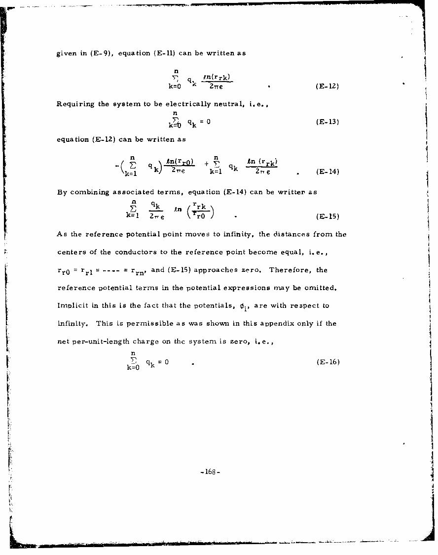
-'_ -.• -- --- r 7

given in (E-9), equation (E-11) can be written as

nn qk .n(r rk)k--02Tre (E- 12)

Requiring the system to be electrically neutral, i.e.,n

k--b k q 0 (E-13)

equation (E-12) can be written as

S 'n(rr) + ' qk rk)"" k 2 re k=l 2TT C (E- 14)

By combining associated terms, equation (E-14) can be writter ask• qk¶ rk

I ~nk1l 2Ze rO /0 (E- 15)

As the reference potential point moves to infinity, the distances from the

centers of the conductors to the reference point become equal, i.e.

rr0 rrl-- - rrn, and (E-15) approaches zero. Therefore, the

reference potential terms in the potential expressions may be omitted.

Implicit in this is the fact that the potentials, OP are with respect to

infinity. This is permissible as was shown in this appendix only if the

net per-unit-length charge on thc system is zero, i.e.,

n

q~ 0~= (E- 16)k=0

-168- j

REFERENCES

fi] S. Hayashi, Surges on Transmission Systems. Kyoto, Japan: Denki-Shoin, Inc., 1955.

rZ] W. C. Johnson, Transmission Lines and Networks. New York:McGraw-Hill, 1950.

[3] J. Zaborszky and J. W. Rittenhouse, Electric Power Transmission.New York: Ronald Press, 1954.

[4] L. A. Pipes, "M.atrix Theory of Multiconductor Transmission Lines",Phil. Mag., Vol. 24, No. 159, pp. 97-113, July 1937.

[5] L. A. Pipes, "Steady-State Analysis of Multi-Conductor Transmis-sion Lines", Jour. Appl. Phys., Vol. 12, No. 11, pp. 782-789,November 1941.

[6] H. W. Dommel and W. S. Meyer, "Computation of ElectromagneticTransients", Proc. IEEE, Vol. 62, No. 7, pp. 983-993, July 1974.

[7] R. H. Galloway, W. B. Shorrocks, and L. M. Wedepohl, "Calcula-tion of Electrical Parameters for Short and Long Polyphase Trans-mission Lines", Proc. IEE, Vol. l11, No. 12, pp. 2051-2059,December 1964.

[8] D. E. Hedman, "Propagation on Overhead Transmission Lines I -

Theory of Modal Analysis 11 - Earth-Conduction Effects and PracticalResults", Trans. IEEE, Vol. PAS-84, pp. 200-211, March 1965.

[9] W. I. Bowman and J. M. McNamee, "Development of EquivalentPi and T Matrix Circuits for Long Untransposed Transmission Lines",IEEE Trans. on Power Apparatus and Systems, pp. 625-632, June

1964.

[10] M. Ushirozawa, "High- Frequency Propagation on NontransposedPower Line", Tranis. IEEE , Vol. 83, pp. 1137-1145, November, 1964.

[il] P.Chowdhuri and E. T. B. Gross, "Voltages Induced on OverheadMulticonductor Lines by Lightning Strokes", Proc. IEE, Vol. 116,No. 4, pp, 561-565, April 1969.

[12] L. M. Wedepohl, "Application of Matrix Methods to the Solution ofTraveling Wave Phenomena in Polyphase Systems", Proc. LEE,Vol. 110, No. 12, pp. 2200-2212, December 1963.

-169-

• -J

[13] C. R. Paul, "Solution of the Transmission Line Equations for LossyConductors and Imperfect Earth," Proc. IEE(London), VoL 122,

No. 2, pp. 177-182, February 1975.

[14] F. Y. Chang and 0. Wing, "Multilayer RC Distributed Networks",IEEE Trans. Circuit Theory, Vol. CT-17, pp. 32-40, February 1970.

[15] F. Y. Chang, "Transient Analysis of Lossless Coupled TransmissionLines in Inhomogeneous Dielectric Medium", IEEE Trans. MicrowaveTheory and Tech., Vol. MTT-18, No. 9, pp. 616-626, September 1970.

[16] K. D. Marx, "Propagation Modes, Equivalent Circuits, and Charac-teristic Terminations for Multiconductor Transmission Lines with

Inhomogeneous Dielectrics", IEEE Trans. Microwave Theory andTech., Voi. MTT-21, No. 7, pp. 450-457, July 1973.

[17] C. W. Ho, "Theory and Computer-Aid d Analysis of Lossless Trans-mission Lines", IBM J. Research and Develop., pp. 249-255, May

1973.

[18] C. R. Paul, "Useful Matrix Chain Parameter Identities for theAnalysis of Multiconductor Transmission Lines", IEEE Trans. on

Microwave Theory and Techniques, Vol. MTT-23, No. 9, pp. 756-

760, September 1975.

fI0] E. Ott, A Network Approach to the Design of Multi-line ZN-PortDirectional Couplers, Rome Air Development Center, Griffiss AFB,

New York, RADC-TR-65-41, April 1965. (AD614 650)

[20] C. D. Taylor, R. S. Satterwhite and C. W. Harrison, Jr., "The

Response of a Terminated Two-Wire Transmission Line Excited bya Nonuniform Electromagnetic Field", IEEE Trans. on Antennas and

Propagation, pp. 987-989, November 1965.

[21] A. A. Smith, "A More Convenient Form of the Equations for the

Response of a Transmission Line Excited by Nonuniform Fields",IEEE Trans. Electromagnetic Compatibility, Vol. EMC-15, pp. 151-152, August 1973.

[22] Electromagnetic Pulse Handbook for Missles and Aircraft in Flight,Sandia Laboratories, SC-M-710346, Albuquerque, N. M., September1972.

-170-

... I,

I

[23] Aeronautical Systems EMP Technology Review (Chapter 5), The

Boeing Con pany, Aerospace Group, Boeing Document D224-10004-1,April 15, 1972.

(24] C. W. Harrison, Jr., "Generalized Theory of Impedance Loaded Mul-ticonductor Transmission Lines in an Incident Field," IEEE Trans.on Electromagnetic Compatibility, Vol. EMC-14, No.2, pp. 56-63, May

' ~197Z.

[25] S. Frankel, "Terminal Response of Braided-Shield Cables to Exter-nal Monochromatic Electromagnetic Fields", IEEE Trans. on

Electromagnetic Compatibility, Vol. EMC-16, No. 1, pp. 4-16,

February 1974.

[26] C. R. Paul, "Efficient Numerical Computation of the Frequency

Response of Cables Illuminated by an Electromagnetic Field", IEEE

Trans. on Microwa-ve Theory and Tech., Vol. MTT-2Z, No. 4,pp. 454-457, April 1974.

[27] C. R. Paul, "Frequency Response of Multiconductor Transmission

Lines Illuminated by an Electromagnetic Field", 1975 IEEE Interna-

tional Symposium on Electromagnetic Compatibility, San Antonio,

Texas, October 1975.

[28] J. C. Isaacs, Jr. and N. A. Strakhov, "Crosstalk in Uniformly

Coupled Lossy Transmission Lines", Bell System Tech. J., Vol. 52,

No. 1, pp. 101-115, January 1973.

[291 J. R. Carson, "Wave Propagation in Overhead Wires With Ground

Return", Bell Syst. Tech. J. , Vol. 5, pp. 539-559, 1926.

[30] R. E. Matick, Transmission Lines for Digital and CommunicationNetworks. New York: McGraw-Hill, 1969.

[31] W. T. Weeks, "Mathematical Analysis of Ferrite Core Memory

Arrays", IEEE Trans. on Computers, Vol. C-18, No. 5, pp. 409-

416, May 1969.

[32] K. A. Chen, "Computer-Aided Memory Design Using TransmissionLine Models", IEEE Trans. on Computers, Vol. C-17, No. 7,pp. 640-648, July 1968.

[33] B. L. Carfson, W. R. Marcelja and D. A. King, Computer Analysisof Cable Coupling for Intra-syste Electromagnetic Compatibility

AFAL-TR-65-142, Wright Patterson AFB, Ohio, The Boeing Com-

pany, May 1965.

-171-

itA

[34] J. Bogdanor, M. Siegel and G. Weinstock, Intra-vehicle Electro-magnetic Compatibility Analysis, AFAL Contract No.F33615-70-C-1333, Wright Patterson AFB, Ohio. The McDonnell-Douglas Corporation, April 1971.

[35] W. R. Johnson, A. K. Thomas, et. al., Development of a SpaceVehicle Electromagnetic Interference /Comrratibilit- Specification,NASA Contract Number 9-7305, The TRW Company08900-6001-TOOO, June 1968.

[36] Digital Computer Program for EMR. Effects on Electronic Systems,Test and Reliability Evaluation Laboratory, U. S. Army MissleCommand, Contract DAA HOI-69-C-1381, GTE Sylvania Incorporated,June 1972.

[37] J. L. Bogdanor, R. A. Pearlman and M. D. Siegel, IntrasystemElectromagnetic Compatibility Analysis Program, Technical Report,RADC-TR-74-342 Rome Air Development Center, Griffiss AFB,N.Y., December 1974. Vols I - III (AD A008 526 - A008528)

[38] C. R. Paul, Linear Systems, Technical Report, RADC-TR-71-134,

Rome Air Development Center, Griffiss AFB, N. Y., July 1971.(AD728 631)

[39] R. M. Fano, L. J. Chu and R. B. Adler, Electromagnetic Fields,Energy and Forces. New York: Wiley, 1960.

[40] R. B. Adler, L. J. Chu and R. M. Fano, Electromagnetic EnergyTransmission and Radiation. New York: Wiley, 1960.

[41] F. E. Hohn, Elementary Matrix Algebra. New York: Macmillan,Second Edition, 1964.

[42] K. Ogata, State Space Analysis of Control Systems. EnglewoodCliffs, N. J.: Prentice-Hall, 1967.

[43] E. N. Protonotarios and 0. Wing, "Analysis and Intrinsic Propertiesof the General Nonuniform Transmission Line", IEEE Trans. onMicrowave Theory Tech., Vol. MTT-15, No. 3. pp. 142-150, March1967.

[44] K. Singhal and 0. Wing, "Network Functions of a Class of Non-uniform Multi-layer Distributed Networks", IEEE Trans. CircuitTheory, Vol. CT-17, No. 2, pp. 275-277, May 1970.

-172-

-Hmmmlw -&0101

145] H. Hagiwara and S. Okugawa, "Time-Domain Analysis of Multicon-ductor Exponential Lines", Proceedings IEEE, pp. 1111-1112, June

1968.

[46] E. C. Bertnolli, "Analysis of the N-Wire Exponential Line",

Proceedings IEEE, pp. 1225, June 1967.

[47] C. R. Paul, "On Uniform Multimode Transmission Lines", IEEETrans. Microwave Theory and Techniques, Vol. MTT-21, No. 8,

pp. 556-558, August 1973.

[48] C. R. Paul and J. C. Clemenfs, "Coupled Transmission Lines",1972 IEEE SOUTHEAST-CON, Louisville, Ky., May 1972.

[49] A. Ralston, A First Course in Numerical Analysis. New York:McGraw-Hill, 1965.

[50] System/360 Scientific Subroutine Package, Version III, Fifth Edition,International Business Machines Curporation, TeLhnical PublicationsDepartment, 112 East Post Road, White Plains, New York, August

1970.

r51] R. L. Goldberg, "Focus on Flexible Flat Cable and PC's", Electron-ic Design, Vol. 20, No. 25, pp. 60-68, December 7, 1972.

[52] D. F. Strawe, Analysis of Uniform Symmetric Transmission Lines,The Boeing Company, Boeing Document, D2-19734-1, August 1971.

[53] A. ML Erisman and G. E. Spie(s, "Exploiting Problem Characteristics

in the Sparse Matrix Approach to Frequency Domain Analysis",

IEEE Trans. Circuit Theory, Vol. CT-19, No. 3, pp. 260-264, May1972.

[54] W. T. Weeks, "Multiconductor Transmission Line Theory in theTEM Approximation", IBM J. Research and Development, pp. 604-611, November 1972.

[55] W. B. Boast, Vector Fields. New York: Harper & Row, Second

Edition, 1964.

[56] J. C. Clements and C. R. Paul, Computation of the CapacitaxhceMatrix for Dielectric-Coated Wires, Technical Report, TR-'t4-59,Rome Air Development Center, Griffiss AFB, N. Y., March 1974.

(AD 778 '4.8)

-173-

IArm

[57] J. C. Clements, C. R. Paul and A. T. Adams, "Computation of theCapacitance Matrix for Systemns of Dielectric-Coated CylindricalConductors", IEEE Trans. on Electromagnetic Compatibility, Vol.

EMC-17, No. 4, pp. 238-248, November 1975.

f58] A. T. Adams, Electromagnetics for Engineers. New York: RonaldPress, 1971.

r59] A. T. Adams and J. R. Mautz, "Computer Solution of ElectrostaticField Problems by Matrix Inversion", Proceedings 1969 NationalElectronics Conference, pp. 198-201.

160] M. P. Sarma, "Application of Moment Methods to the Computationof Electrostatic Fields-Part I - Parallel Cylindrical ConductorSystems", IEEE PES Summer Meeting, San Francisco, CA., July9-14, 1972.

[61] D. W. Kammler, "Calculation of Characteristic Admittances andCoupling Coefficients for Strip Transmission Lines", IEEE Trans.Microwave Theory Tech., Vol. MTT-16, No. 11, pp. 925-937,November 1968.

[62] J. W. Craggs, "The Determination of Capacity for Two-DimensionalSystems of Cylindrical Conductors", Quarterly J. of Mathematics(Oxford Series), Vol. 17, pp. 131-137, 1946.

[63] M. P. Sarma and W. Janischewskyj, "Electrostatic Field of a Systemof Parallel Cylindrical Conductors", IEEE Trans. on Power Apara-tus and Systems, Vol. PAS-88, No. 7, pp. 1069-1079, July 1969.

[64) M. S. Abou - Seada and E. Nasser, "Digital Computer Calculation ofthe Potential and its Gradient of a Twin Cylindrical Conductor",IEEE Trans. on Power Apparatus and Systems, Vol. PAS-88, No. 12,pp. 1802-id14, December 1969.

[65] A. Mattumoto, Network Synthesis with Multiwire Lines, RADC-TDR-63- 369, Rome Air Development Center, Griffiss AEB, N. Y., Auguist1963. (AD 417 757)

[66] J. W. Craggs and C. J. Tranter, "The Capacity of Two-DimensionaluSystems of Conductors and Dielectrics With Circular Bou)daries",

SQuarterly J. of Mathematics (Oxfoad Series), Vol. 17, pp. 138-144,1946.

-174-

OK~

II

[671 W. T. Weeks, "Calculation of Coefficients of Capacitance of Multi-conductor Transmission Lines in the Presence of a Dielectric Inter-

face, " IEEE Trans. Microwave Theory Tech., Vol. MTT-18, p. 35,19"0.

[68] L. Young, Parallel Coupled Lines and Directional Couplers. Dedham,Mass: Artech House, 1972.

A17

-175-

MIS:S:ION

BMWa Air Devmiopwweant Cenier

XADC as the FrInaljoil AFSC ormAnj adt la cierged tiPlannzt; &Mi ocat lg the VL.A explorabm-fj wWadM nvdava.aadwt pad:m faor inhigma tion sci@Awex. inal . . I-

k~-iwitv a~nd servicvs aximinted to tiW ne..d of the L5F.Primary 5AW misio ga &~ Zve are ca0.u"J C i WW, e-Dog tic quild-n and owatrl. sur liaIKcv 0.C qro~a'&d~acop AOXWWOCjjCt&, int4UIilgW* datJa Co.J4,Ci"ki &4bMndliig, istfaou~tio syst.m t~chwaojxogV, iane wjactkx\ýaUr*Iidb4Zity, awlataintbility anad C a bia.RA.CA

S has makaicm re.pwnaibii 1t y asu -asi gnoc b4 AFSC fc~r cia-monstxrstion and ac.qwstaa.niv of sa.Iected Azhevst &ftsyatin IA the Lnt.*llqmmw-o, mopping, chkrawri, "Mai4,omtzwJ n ~ lcat lme xreas.