©1999 crc press llc - freeebrary.free.fr/mesh generation/handbook_of_grid_ generation,1999... ·...

Acquiring Editor: B. SternProject Editor: Sylvia WoodMarketing Manager: J. Stark


Cover design: Dawn BoydManufacturing Manager: Carol Slatter

Library of Congress Cataloging-in-Publication Data

Thompson, Joe F.Handbook of Grid Generation / Joe F. Thompson, Bharat Soni, Nigel

Weatherill, editors. p. cm.

Includes bibliographical references and index.ISBN 0-8493-2687-7 (alk. paper)1. Numerical grid generation (Numerical analysis) I. Thompson,

Joe F. II. Soni, B.K. III. Weatherill, N.P.QA377.H3183 1998519.4--dc21 98-34260

CIP

This book contains information obtained from authentic and highly regarded sources. Reprinted material is quoted withpermission, and sources are indicated. A wide variety of references are listed. Reasonable efforts have been made to publishreliable data and information, but the author and the publisher cannot assume responsibility for the validity of all materialsor for the consequences of their use.

Neither this book nor any part may be reproduced or transmitted in any form or by any means, electronic or mechanical,including photocopying, microfilming, and recording, or by any information storage or retrieval system, without priorpermission in writing from the publisher.

All rights reserved. Authorization to photocopy items for internal or personal use, or the personal or internal use ofspecific clients, may be granted by CRC Press LLC, provided that $.50 per page photocopied is paid directly to CopyrightClearance Center, 27 Congress Street, Salem, MA 01970 USA. The fee code for users of the Transactional Reporting Serviceis ISBN 0-8493-2687-7/99/$0.00+$.50. The fee is subject to change without notice. For organizations that have been granteda photocopy license by the CCC, a separate system of payment has been arranged.

The consent of CRC Press LLC does not extend to copying for general distribution, for promotion, for creating newworks, or for resale. Specific permission must be obtained in writing from CRC Press LLC for such copying.

Direct all inquiries to CRC Press LLC, 2000 Corporate Blvd., N.W., Boca Raton, Florida 33431.

Trademark Notice: Product or corporate names may be trademarks or registered trademarks, and are used only foridentification and explanation, without intent to infringe.

© 1999 by CRC Press LLC

No claim to original U.S. Government worksInternational Standard Book Number 0-8493-2687-7Library of Congress Card Number 98-34260Printed in the United States of America 1 2 3 4 5 6 7 8 9 0Printed on acid-free paper

Foreword


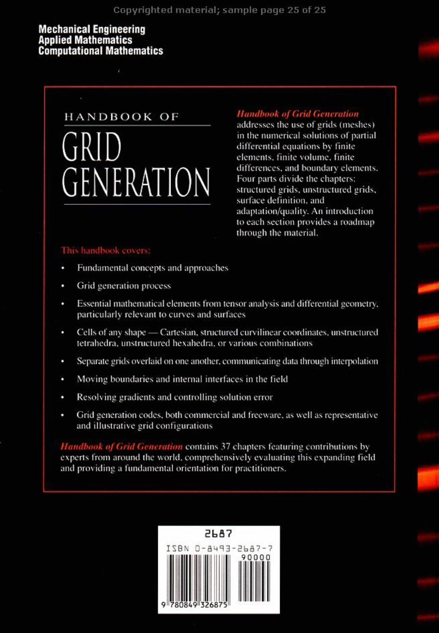
Grid (mesh) generation is, of course, only a means to an end: a necessary tool in the computationalsimulation of physical field phenomena and processes. (The terms grid and mesh are used interchangeably,with identical meaning, throughout this handbook.)

And grid generation is, unfortunately from a technology standpoint, still something of an art, as wellas a science. Mathematics provides the essential foundation for moving the grid generation process froma user-intensive craft to an automated system. But there is both art and science in the design of themathematics for — not of — grid generation systems, since there are no inherent laws (equations) ofgrid generation to be discovered. The grid generation process is not unique; rather it must be designed.There are, however, criteria of optimization that can serve to guide this design.

The grid generation process has matured now to the point where the use of developed codes — freewareand commercial — is generally to be recommended over the construction of grid generation codes byend users doing computational field simulation. Some understanding of the process of grid generation— and its underlying principles, mathematics, and technology — is important, however, for informedand effective use of these developed systems. And there are always extensions and enhancements to bemade to meet new occasions, especially in coupling the grid with the solution process thereon.

This handbook is designed to provide essential grid generation technology for practice, with sufficientdetail and development for general understanding by the informed practitioner. Complete details for thegrid generation specialist are left to the sources cited. A basic introduction to the fundamental conceptsand approaches is provided by Chapter l, which covers the state of practice in the entire field in a verybroad sweep. An even more basic introduction for those with little familiarity with the subject is givenby the Preface that precedes this first chapter. Appendixes provide information on a number of availablegrid generation codes, both commercial and freeware, and give some representative and illustrative gridconfigurations.

The grid generation process in general proceeds from first defining the boundary geometry as discussedin Part III. Points are distributed on the curves that form the edges of boundary sections. A surface gridis then generated on the boundary surface, and finally, a volume grid is generated in the field. Chapter 13,although directed at structured grids, gives a general overview of the entire grid generation process andthe fundamental choices and considerations involved from the standpoint of the user. Chapter 2, thoughalso largely directed at structured grids, covers essential mathematical elements from tensor analysis anddifferential geometry relevant to the entire subject, particularly the aspects of curve and surfaces.

The other chapters of this handbook cover the various aspects of grid generation in some detail, butstill from the standpoint of practice, with citations of relevant sources for more complete discussion ofthe underlying technology. The chapters are grouped into four parts: structured grids, unstructured grids,surface definition, and adaptation/quality. An introduction to each part provides a road map throughthe material of the chapters.

A source of fundamentals on structured grid generation is the 1985 textbook of Thompson, Warsi,and Mastin, now out of print but accessible on the Web at www.erc.msstate.edu. A recent comprehensivetext of both structured and unstructured grids is that of Carey 1997 from Taylor and Francis publishers.

http://www.erc.msstate.edu

The first step in generating a grid is, of course, to acquire and input the boundary data. This boundarydata may be in the form of output from a CAD system, or may simply be sets of boundary points acquired


from drawings. CAD boundary data are generally in the form of some parametric description of boundarycurves and surfaces, typically consisting of multiple segments for which assembly and some adjustmentsmay be required. Point boundary data may be in the form of 1D arrays of points describing boundarycurves and 2D arrays for boundary surfaces, or could be an unorganized cloud of points on a surface.In the latter case, conversion to some surface tessellation or parametric description is required. Theseinitial steps of boundary definition are common in general to both structured and unstructured gridgeneration. And, unfortunately, considerable human intervention may be necessary in this setup phaseof the process.

The setup of the boundary definition from the CAD approach is discussed in general in Chapter 13,while details of application, together with procedures for boundary curve and surface parametric repre-sentations, are covered in Part III. There is then the fundamental choice of whether to use a structuredor unstructured grid. Structured grids are covered in Part I, and unstructured grids are covered in Part II.

The next step with either type of grid is the generation of the corresponding type of grid on theboundary surfaces — preceded, of course, by a distribution on points on the curves that form the edgesof these surfaces. This surface grid generation is covered in Chapters 9 and 19 for structured andunstructured grids, respectively.

Finally, the quality of the grid, with relation to the accuracy of the numerical solution being done onthe grid, and the adaptation of the grid to improve that accuracy are covered in Part IV.

Grid generation is still under active research and development, particularly in regard to automation,adaptation, and hybrid combinations. This handbook is therefore necessarily a snapshot in time, espe-cially in these areas, but much of the material has matured now, and this collection should be of enduringvalue as a source and reference.

Bharat K. SoniJoe F. Thompson

Nigel P. Weatherill

Starkville, MS, and Swansea, Wales, UK

Contributors

Michael J. AftosmisNASA Ames Research CenterMoffett Field, CA

Timothy J. BakerPrinceton UniversityPrinceton, NJ

Mark W. BeallRensselaer Polytechnic InstituteTroy, NY

Marsha J. BergerCourant InstituteNew York University

William M. ChanMCAT, Inc. at NASA Ames

Research CenterMoffett Field

Zheming ChengProgram Development

CorporationWhite Plains, NY

Hugues L. de CougnyRensselaer Polytechnic InstituteTroy, NY

Luís EçaTechnical University of LisbonLisbon, Portugal

Peter R. EisemanProgram Development CorporationWhite Plains, NY

Austin L. EvansNASA Lewis Research CenterCleveland, OH

Gerald FarinArizona State UniversityTempe, AZ

David R. FergusonThe Boeing CompanySeattle, WA

Luca FormaggiaEcole Polytechnique Federale de

LausanneLausanne, Switzerland

Timothy GatzkeThe Boeing CompanySt. Louis, MO

Paul-Louis GeorgeINRIALe Chesnay Cedex, France

Bernd HammannUniversity of California at DavisDavis, CA

O. HassanUniversity of Wales SwanseaSwansea, UK

Jochem HäuserCLE Salzgitter BadSalzgitter, Germany

Frédéric HechtINRIALe Chesnay Cedex, France

Sergey A. IvanenkoComputer Center of the Russian

Academy of SciencesMoscow, Russia

Olivier-Pierre JacquotteResearch Directorate (DRET)Paris, France

Brian A. JeanU.S. Army Corps of Engineers

Waterways Experiment StationVicksburg, MS

Yannis KallinderisUniversity of TexasAustin, TX

O.B. KhairullinaUrals Branch of the Russian

Academy of SciencesEkaterinburg, Russia

Ahmed KhamaysehLos Alamos National LaboratoryLos Alamos, NM

Andrew KupratLos Alamos National LaboratoryLos Alamos, NM

Kelly R. LaflinNorth Carolina State UniversityRaleigh, NC

Kunwoo LeeSeoul National UniversitySeoul, Korea

David L. MarcumMississippi State UniversityStarkville, MS

C. Wayne MastinNichols Research CorporationVicksburg, MS


D. Scott McRae

North Carolina State UniversityRaleigh, NC

E. J. Probert

University of Wales SwanseaSwansea, UK

Joe F. Thompson

Mississippi State UniversityStarkville, MS


Robert L. MeakinArmy Aeroflightdynamics

Directorate (AMCOM)Moffett Field, CA

John E. MeltonNASA Ames Research CenterMoffett Field, CA

David P. MillerNASA Lewis Research CenterCleveland, OH

K. MorganUniversity of Wales SwanseaSwansea, UK

Robert M. O’BaraRensselaer Polytechnic InstituteTroy, NY

Sangkun ParkInformation Technology R&D

CenterSeoul, Korea

J. PeraireMassachusetts Institute

of TechnologyCambridge, MA

J. PeiróImperial CollegeLondon, UK

Anshuman RazdanArizona State UniversityTempe, AZ

Robert SchneidersMAGMA Giessereitechnologie

GmbHAachen, Germany

Jonathon A. ShawAircraft Research AssociationBedford, U.K.

A.F. SidorovUrals Branch of the Russian


Mark S. ShephardRensselaer Polytechnic InstituteTroy, NY

Robert E. SmithNASA Langley Research CenterHampton, VA

Bharat K. SoniMississippi State UniversityStarkville, MS

Stefan P. SpekreijseNational Aerospace Laboratory

(NLR)Emmeloord, The Netherlands

O.V. UshakovaUrals Branch of the Russian


Zahir U.A. WarsiMississippi State UniversityStarkville, MS

Nigel P. WeatherillUniversity of Wales SwanseaSwansea, UK

Yang XiaCLE Salzgitter BadGermany

Tzu-Yi YuChaoyang University of TechnologyWufeng, Taiwan

Paul A. ZegelingUniversity of UtrechtUtrecht, The Netherlands

Acknowledgments


Grid (mesh) generation is truly a worldwide active research area of computation science, and thishandbook is the work of individual authors from around the world. It has been a distinct pleasure, andan opportunity for professional enhancement, to work with these dedicated researchers in the course ofthe preparation of this book over the past two years. The material comes from universities, industry, andgovernment laboratories in 10 countries in North America, Europe, and Asia. And we three are fromthree different countries of origin, though we have collaborated for years.

The attention to quality that has been the norm in the authoring of these many chapters has madeour editing responsibility a straightforward process. These chapters should serve well to present thecurrent state of the art in grid generation to practitioners, researchers, and students.

The assembly and editing of the material for this handbook from all over the world via the Internethas been a rewarding experience in its own right, and speaks well for the potential for worldwidecollaborative efforts in research.

Our thanks go to Mississippi State University and the University of Wales Swansea for the encourage-ment and support of our efforts to produce this handbook. Specifically at Mississippi State, the work ofRoger Smith in administering the electronic communication is to be noted, as are the efforts of AlishaDavis, who handled the word processing.

Bob Stern of CRC Press has been great to work with and appreciation is due to him for recognizingthe need for this handbook and for his editorial guidance and assistance throughout its preparation. Hisefforts, and those of Sylvia Wood, Suzanne Lassandro and Dawn Mesa, also at CRC, have made this apleasant process.

We naturally are especially grateful for the support of our wives, Purnima, Emilie, Barbara, and ourfamilies in this and all our efforts. And finally, Mississippi and Wales — two great places to live and work.

Bharat K. SoniJoe F. Thompson

Nigel P. WeatherillAuthor/Editors

Preface:


An Elementary Introduction

Joe F. Thompson, Bharat K. Soni, and Nigel P. Weatherill

This first section is an elementary introduction provided for those with little familiarity with grid (mesh)generation in order to establish a base from which the technical development of the chapters in thishandbook can proceed. (The terms grid and mesh are used interchangeably throughout with identicalmeaning.) The intent is not to introduce numerical solution procedures, but rather to introduce the ideaof using numerically generated grid (mesh) systems as a foundation of such solutions.

P-1 Discretizations

The numerical solution of partial differential equations (PDEs) requires first the discretization of theequations to replace the continuous differential equations with a system of simultaneous algebraicdifference equations. There are several bifurcations on the way to the construction of the solution process,the first of which concerns whether to represent the differential equations at discrete points or overdiscrete cells. The discretization is accomplished by covering the solution field with discrete points thatcan, of course, be connected in various manners to form a network of discrete cells. The choice lies inwhether to represent the differential equations at the discrete points or over the discrete cells.

P-1.1 Point Discretization

In the former case (called finite difference), the derivatives in the PDEs are represented at the points byalgebraic difference expressions obtained by performing Taylor series expansions of the solution variablesat several neighbors of the point of evaluation. This amounts to taking the solution to be represented bypolynomials between the points. This can be unrealistic if the solution varies too strongly between thepoints. One remedy is, of course, to use more points so that the spacing between points is reduced. This,however, can be expensive, since there will then be more points at which the equations must be evaluated.

This is exacerbated if the points are equally spaced and strong variations in the solution occur overscattered regions of the field, since numerous points will be wasted in regions of small variation. Analternative, of course, is to make the points unequally spaced.

P-1.2 Cell Discretization

The other possibility of this first bifurcation is to return the PDEs to their more fundamental integralform and then to represent the integrals over discrete cells. Here there is yet another bifurcation —whether to represent the solution variables over the cell in terms of selected functions and then to integrate


these functions analytically over the volume (finite element), or to balance the fluxes through the cellsides (finite volume).

The finite element approach itself comes in two basic forms: the variational, where the PDEs arereplaced by a more fundamental integral variational principle (from which they arise through the calculusof variations), or the weighted residual (Galerkin) approach, in which the PDEs are multiplied by certainfunctions and then integrated over the cell.

In the finite volume approach, the solution variables are considered to be constant within a cell, andthe fluxes through the cell sides (which separate discontinuous solution values) are best calculated witha procedure that represents the dissolution of such a discontinuity during the time step (Riemann solver).

P-2 Curvilinear (Structured) Grids

The finite difference approach, using the discrete points, is associated historically with rectangularCartesian grids, since such a regular lattice structure provides easy identification of neighboring pointsto be used in the representation of derivatives, while the finite element approach has always been, by thenature of its construction on discrete cells of general shape, considered well suited for irregular regions,since a network of such cells can be made to fill any arbitrarily shaped region and each cell is an entityunto itself, the representation being on a cell, not across cells.

P-2.1 Boundary-Fitted Grids

The finite difference method is not, however, limited to rectangular grids and has long been applied onother readily available analytical coordinate systems (cylindrical, spherical, elliptical, etc.) that still forma regular lattice. albeit curvilinear, that allows easy identification of neighboring points. These specialcurvilinear coordinate systems are all orthogonal, as are the rectangular Cartesian systems, and they alsocan exactly cover special regions (e.g., cylindrical coordinates covering the annular region between twoconcentric circles) in the same way that a Cartesian grid fills a rectangular region. The cardinal featurein each case is that some coordinate line is coincident with each portion of the boundary.

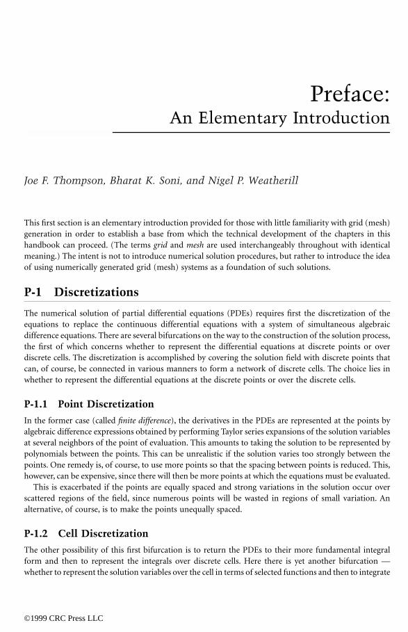
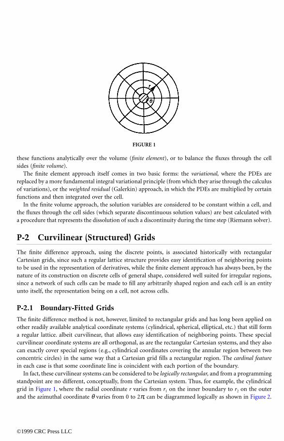
In fact, these curvilinear systems can be considered to be logically rectangular, and from a programmingstandpoint are no different, conceptually, from the Cartesian system. Thus, for example, the cylindricalgrid in Figure 1, where the radial coordinate r varies from r1 on the inner boundary to r2 on the outerand the azimuthal coordinate θ varies from 0 to 2π, can be diagrammed logically as shown in Figure 2.

FIGURE 1


The continuity of the azimuthal coordinate can be represented by defining extra “phantom” columnsto the left of 0 and to the right of 2π and setting values on each phantom column equal to those on thecorresponding “real” columns inside of 2π and 0, respectively. This latter, logically rectangular, view ofthe cylindrical grid is the one used in programming anyway, and without being told of the cylindricalconfiguration, a programmer would not realize any difference here from programming in Cartesiancoordinates — there would simply be a different set of equations to be programmed on what is still alogically rectangular grid, e.g., the Laplacian on a Cartesian grid (with ξ = x and η = y),

becomes (with ξ = θ and η = r)

on a cylindrical grid. The key point here is that in the logical (i.e., programming) sense there is reallyno essential difference between Cartesian grids and the cylindrical systems: both can be programmed asnested loops; the equations simply are different.

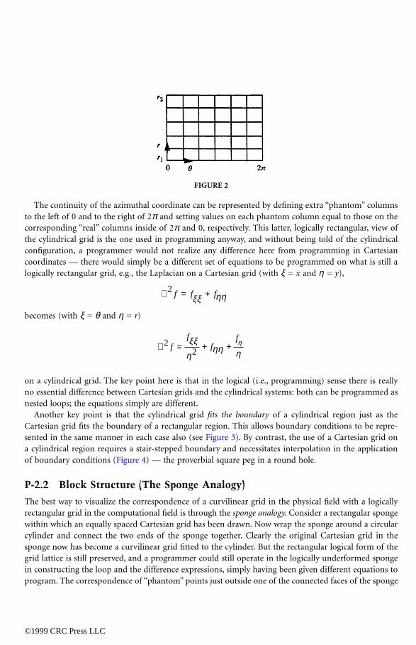
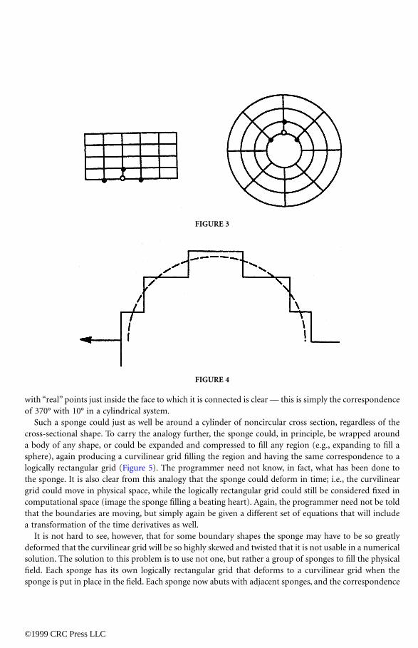
Another key point is that the cylindrical grid fits the boundary of a cylindrical region just as theCartesian grid fits the boundary of a rectangular region. This allows boundary conditions to be repre-sented in the same manner in each case also (see Figure 3). By contrast, the use of a Cartesian grid ona cylindrical region requires a stair-stepped boundary and necessitates interpolation in the applicationof boundary conditions (Figure 4) — the proverbial square peg in a round hole.

P-2.2 Block Structure (The Sponge Analogy)

The best way to visualize the correspondence of a curvilinear grid in the physical field with a logicallyrectangular grid in the computational field is through the sponge analogy. Consider a rectangular spongewithin which an equally spaced Cartesian grid has been drawn. Now wrap the sponge around a circularcylinder and connect the two ends of the sponge together. Clearly the original Cartesian grid in thesponge now has become a curvilinear grid fitted to the cylinder. But the rectangular logical form of thegrid lattice is still preserved, and a programmer could still operate in the logically underformed spongein constructing the loop and the difference expressions, simply having been given different equations toprogram. The correspondence of “phantom” points just outside one of the connected faces of the sponge

FIGURE 2

∇ = +2f f fξξ ηη

∇ = + +22f

ff

fξξη

ηη ηη

with “real” points just inside the face to which it is connected is clear — this is simply the correspondenceof 370° with 10° in a cylindrical system.

Such a sponge could just as well be around a cylinder of noncircular cross section, regardless of thecross-sectional shape. To carry the analogy further, the sponge could, in principle, be wrapped arounda body of any shape, or could be expanded and compressed to fill any region (e.g., expanding to fill asphere), again producing a curvilinear grid filling the region and having the same correspondence to alogically rectangular grid (Figure 5). The programmer need not know, in fact, what has been done tothe sponge. It is also clear from this analogy that the sponge could deform in time; i.e., the curvilineargrid could move in physical space, while the logically rectangular grid could still be considered fixed incomputational space (image the sponge filling a beating heart). Again, the programmer need not be toldthat the boundaries are moving, but simply again be given a different set of equations that will includea transformation of the time derivatives as well.

It is not hard to see, however, that for some boundary shapes the sponge may have to be so greatlydeformed that the curvilinear grid will be so highly skewed and twisted that it is not usable in a numericalsolution. The solution to this problem is to use not one, but rather a group of sponges to fill the physicalfield. Each sponge has its own logically rectangular grid that deforms to a curvilinear grid when thesponge is put in place in the field. Each sponge now abuts with adjacent sponges, and the correspondence

FIGURE 3

FIGURE 4


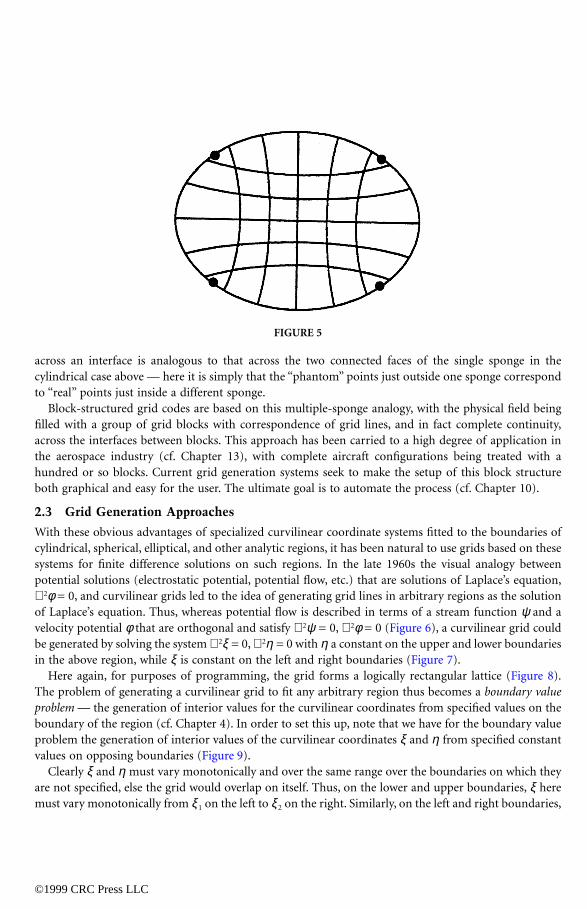
across an interface is analogous to that across the two connected faces of the single sponge in thecylindrical case above — here it is simply that the “phantom” points just outside one sponge correspondto “real” points just inside a different sponge.

Block-structured grid codes are based on this multiple-sponge analogy, with the physical field beingfilled with a group of grid blocks with correspondence of grid lines, and in fact complete continuity,across the interfaces between blocks. This approach has been carried to a high degree of application inthe aerospace industry (cf. Chapter 13), with complete aircraft configurations being treated with ahundred or so blocks. Current grid generation systems seek to make the setup of this block structureboth graphical and easy for the user. The ultimate goal is to automate the process (cf. Chapter 10).

2.3 Grid Generation Approaches

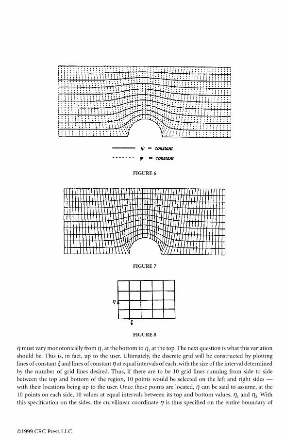
With these obvious advantages of specialized curvilinear coordinate systems fitted to the boundaries ofcylindrical, spherical, elliptical, and other analytic regions, it has been natural to use grids based on thesesystems for finite difference solutions on such regions. In the late 1960s the visual analogy betweenpotential solutions (electrostatic potential, potential flow, etc.) that are solutions of Laplace’s equation,∇ 2φ = 0, and curvilinear grids led to the idea of generating grid lines in arbitrary regions as the solutionof Laplace’s equation. Thus, whereas potential flow is described in terms of a stream function ψ and avelocity potential φ that are orthogonal and satisfy ∇ 2ψ = 0, ∇ 2φ = 0 (Figure 6), a curvilinear grid couldbe generated by solving the system ∇ 2ξ = 0, ∇ 2η = 0 with η a constant on the upper and lower boundariesin the above region, while ξ is constant on the left and right boundaries (Figure 7).

Here again, for purposes of programming, the grid forms a logically rectangular lattice (Figure 8).The problem of generating a curvilinear grid to fit any arbitrary region thus becomes a boundary valueproblem — the generation of interior values for the curvilinear coordinates from specified values on theboundary of the region (cf. Chapter 4). In order to set this up, note that we have for the boundary valueproblem the generation of interior values of the curvilinear coordinates ξ and η from specified constantvalues on opposing boundaries (Figure 9).

Clearly ξ and η must vary monotonically and over the same range over the boundaries on which theyare not specified, else the grid would overlap on itself. Thus, on the lower and upper boundaries, ξ heremust vary monotonically from ξ 1 on the left to ξ 2 on the right. Similarly, on the left and right boundaries,

FIGURE 5



η must vary monotonically from η1 at the bottom to η2 at the top. The next question is what this variationshould be. This is, in fact, up to the user. Ultimately, the discrete grid will be constructed by plottinglines of constant ξ and lines of constant η at equal intervals of each, with the size of the interval determinedby the number of grid lines desired. Thus, if there are to be 10 grid lines running from side to sidebetween the top and bottom of the region, 10 points would be selected on the left and right sides —with their locations being up to the user. Once these points are located, η can be said to assume, at the10 points on each side, 10 values at equal intervals between its top and bottom values, η1 and η2. Withthis specification on the sides, the curvilinear coordinate η is thus specified on the entire boundary of

FIGURE 6

FIGURE 7

FIGURE 8


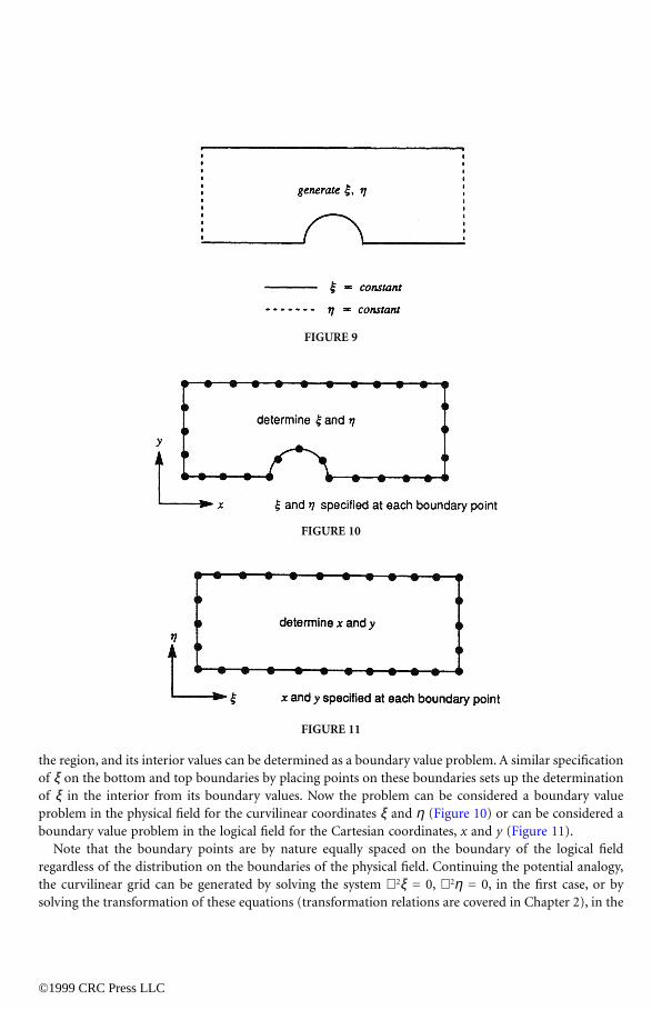
the region, and its interior values can be determined as a boundary value problem. A similar specificationof ξ on the bottom and top boundaries by placing points on these boundaries sets up the determinationof ξ in the interior from its boundary values. Now the problem can be considered a boundary valueproblem in the physical field for the curvilinear coordinates ξ and η (Figure 10) or can be considered aboundary value problem in the logical field for the Cartesian coordinates, x and y (Figure 11).

Note that the boundary points are by nature equally spaced on the boundary of the logical fieldregardless of the distribution on the boundaries of the physical field. Continuing the potential analogy,the curvilinear grid can be generated by solving the system ∇ 2ξ = 0, ∇ 2η = 0, in the first case, or bysolving the transformation of these equations (transformation relations are covered in Chapter 2), in the

FIGURE 9

FIGURE 10

FIGURE 11


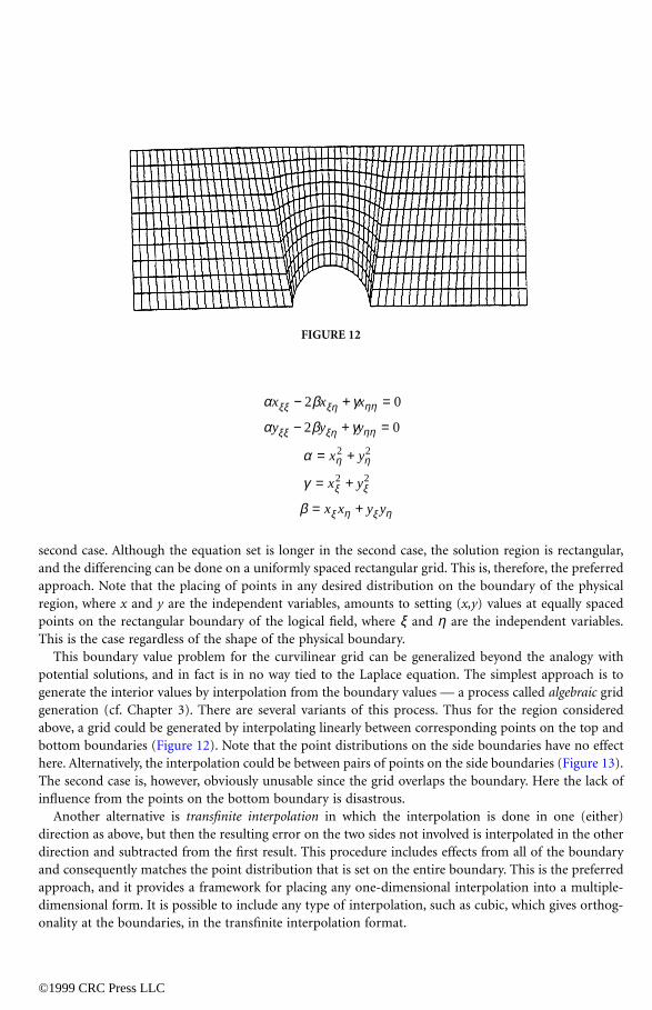
second case. Although the equation set is longer in the second case, the solution region is rectangular,and the differencing can be done on a uniformly spaced rectangular grid. This is, therefore, the preferredapproach. Note that the placing of points in any desired distribution on the boundary of the physicalregion, where x and y are the independent variables, amounts to setting (x,y) values at equally spacedpoints on the rectangular boundary of the logical field, where ξ and η are the independent variables.This is the case regardless of the shape of the physical boundary.

This boundary value problem for the curvilinear grid can be generalized beyond the analogy withpotential solutions, and in fact is in no way tied to the Laplace equation. The simplest approach is togenerate the interior values by interpolation from the boundary values — a process called algebraic gridgeneration (cf. Chapter 3). There are several variants of this process. Thus for the region consideredabove, a grid could be generated by interpolating linearly between corresponding points on the top andbottom boundaries (Figure 12). Note that the point distributions on the side boundaries have no effecthere. Alternatively, the interpolation could be between pairs of points on the side boundaries (Figure 13).The second case is, however, obviously unusable since the grid overlaps the boundary. Here the lack ofinfluence from the points on the bottom boundary is disastrous.

Another alternative is transfinite interpolation in which the interpolation is done in one (either)direction as above, but then the resulting error on the two sides not involved is interpolated in the otherdirection and subtracted from the first result. This procedure includes effects from all of the boundaryand consequently matches the point distribution that is set on the entire boundary. This is the preferredapproach, and it provides a framework for placing any one-dimensional interpolation into a multiple-dimensional form. It is possible to include any type of interpolation, such as cubic, which gives orthog-onality at the boundaries, in the transfinite interpolation format.

FIGURE 12

α β γ

α β γ

α

γ

β

ξξ ξη ηη

ξξ ξη ηη

η η

ξ ξ

ξ η ξ η

x x x

y y y

x y

x y

x x y y

− + =

− + =

= +

= +

= +

2 0

2 0

2 2

2 2


It is still possible in some cases for the grid to overlap the boundaries with transfinite interpolation, andthere is no control over the skewness of the grid. This gives incentive to now return to the grids generatedfrom solving the Laplace equation.

The Laplace equation is, by its very nature, a smoother, tending to average values at points with thoseat neighboring points. It can be shown from the calculus of variations, in fact, that grids generated fromthe Laplace equation are the smoothest possible. There arises, however, the need to concentrate coordinatelines in certain areas of anticipated strong solution variation, such as near solid walls in viscous flow.This can be accomplished by departing from the Laplace equation and designing a partial differentialequation system for grid generation: designing because, unlike physics, there are no laws governing gridgeneration waiting to be discovered.

The first approach to this, historically, was the obvious: simply replace the Laplace equation withPoisson equations ∇ 2ξ = P, ∇ 2η = Q and leave the control functions on the right-hand sides to be specifiedby the user (with appeal to Urania, the muse of science, for guidance). This does in fact work but theapproach has evolved over the years, guided both by logical intuition and the calculus of variations, touse a similar set of equations but with a somewhat different right-hand side. Also, the user has beenrelieved of the responsibility for specifying the control functions, which are now generally evaluatedautomatically by the code from the boundary point distributions that are set by the user (cf. Chapter 4).These functions may also be adjusted by the code to achieve orthogonality at the boundary and/or toreduce the grid skewness or otherwise improve the grid quality (cf. Chapter 6).

Algebraic grid generation, based on transfinite interpolation, is typically used to provide an initialsolution to start an iterative solution of the partial differential equation for this elliptic grid generationsystem that provides a smoother grid, but with selective concentration of lines, and is less likely to resultin overlapping of the boundary.

This elliptic grid generation has an analogy to stretching a membrane attached to the boundaries(cf. Chapter 33) Grid lines inscribed on the underformed membrane move in space as the membrane isselectively stretched, but the region between the boundaries is always covered by the grid. Another formof grid generation from partial differential equations has an analogy with the waves emanating from astone tossed into a pool This hyperbolic grid generation uses a set of hyperbolic equations, rather thanthe Poisson equation, to grow an orthogonal grid outward from a boundary (cf. Chapter 5). This approachis, in fact, faster than the elliptic grid generation, since no iterative solution is involved, but it is notpossible to fit a specified outer boundary. Hyperbolic grid generation is thus limited in its use to openregions. As with the elliptic system, it is possible to control the spacing of the grid lines, and theorthogonality helps prevent skewness.

FIGURE 13

The control of grid line spacing can be extended to dynamically couple the grid generation systemwith the physical solution to be performed on the grid in order to resolve developing gradients in the


solution wherever such variations appear in the field (cf. Chapter 34 and 35). With such adaptive grids,certain solution variables, such as pressure or temperature, are made to feed back to the control functionsin the grid generations system to adjust the grid before the next cycle of the physical solution algorithmon the grid.

P-2.4 Variations

Structured grids today are typically generated and applied in the block-structured form described abovewith the multiple-sponge analogy. A variation is the chimera (from the monster of Greek mythology,composed of disparate parts) approach in which separate grids are generated about various boundarycomponents, e.g., bodies in the field, and these separate grids are simply overlaid on a background gridand perhaps on each other in a hierarchy (cf. Chapter 11). The physical solution process on this compositegrid proceeds with values being transferred between grids by interpolation. This approach has a numberof advantages: (1) simplicity in grid generation since the various grids are generated separately, (2) bodiescan be added to, or taken out of, the field easily, (3) bodies can carry their grids when moving relativeto the background (think of simulating the kicking of a field goal with the ball and its grid tumbling endover end), (4) the separate grids can be used selectively to concentrate points in regions of developinggradients that may be in motion. The disadvantages are the complexity of setup (but this is being attackedin new code development) and the necessity for the interpolation between grids.

Another approach of interest is the hybrid combination with separate structured grids over the variousboundaries, connected by unstructured grids (cf. Chapter 23). There is great incentive to use structuredgrids over boundaries in viscous flow simulation because the boundary layer requires very small spacingout from the wall, resulting either in very long skewed triangular cells or a prohibitively and unnecessarilylarge number of small cells when unstructured grids are used. This hybrid approach is less well developedbut can be expected to receive more attention.

P-2.5 Transformation

The use of numerically generated nonorthogonal curvilinear grids in the numerical solution of PDEs isnot, in principle, any more difficult than using Cartesian grids: the differencing and solution techniquescan be the same; there are simply more terms in the equations. For instance, the first derivative fx couldbe represented in difference form on a Cartesian grid as

or if the spacing is not uniform, though the grid is still rectangular, by

ff f

xx iji j i j( ) =

−∇

+ −1 1

2, ,

ff f

x xx iji j i j

i j i j( ) =

−−

+ −

+ −

1 1

1 1

, ,

, ,

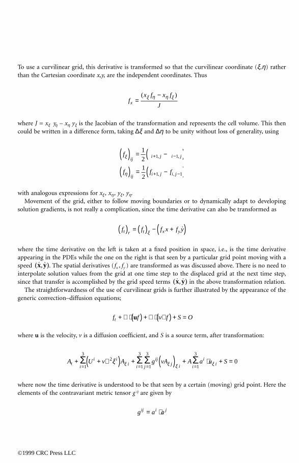
To use a curvilinear grid, this derivative is transformed so that the curvilinear coordinate (ξ,η) ratherthan the Cartesian coordinate x,y, are the independent coordinates. Thus


where J = xξ yη – xη yξ is the Jacobian of the transformation and represents the cell volume. This thencould be written in a difference form, taking ∆ξ and ∆η to be unity without loss of generality, using

with analogous expressions for xξ , xη , yξ , yη.Movement of the grid, either to follow moving boundaries or to dynamically adapt to developing

solution gradients, is not really a complication, since the time derivative can also be transformed as

where the time derivative on the left is taken at a fixed position in space, i.e., is the time derivativeappearing in the PDEs while the one on the right is that seen by a particular grid point moving with aspeed . The spatial derivatives (fx , fy ) are transformed as was discussed above. There is no need tointerpolate solution values from the grid at one time step to the displaced grid at the next time step,since that transfer is accomplished by the grid speed terms in the above transformation relation.

The straightforwardness of the use of curvilinear grids is further illustrated by the appearance of thegeneric convection–diffusion equations;

where u is the velocity, v is a diffusion coefficient, and S is a source term, after transformation:

where now the time derivative is understood to be that seen by a certain (moving) grid point. Here theelements of the contravariant metric tensor g ij are given by

fx f x f

Jx =−( )ξ η η ξ

f

f f f

iji j i j

ij i j i j

ξ

η

( ) = −( )( ) = −( )

+ −

+ −

1

21

2

1 1

1 1

, ,

, ,

f f f x f yt r t x y( ) = ( ) − +( )ξ˙

( ˙, ˙ )x y

( ˙, ˙ )x y

f f v f S Ot + ∇ ⋅ ( ) + ∇ ⋅ ∇( ) + =u

A U v A g vA A a u Sti

i ii

i j

ijj i i

ii+ + ∇( ) + ( ) + ⋅ + =

= = = =Σ Σ Σ Σ

1

32

1

3

1

3

1

3

0ξ ξ ξ ξ ξ

g a aij i j= ⋅

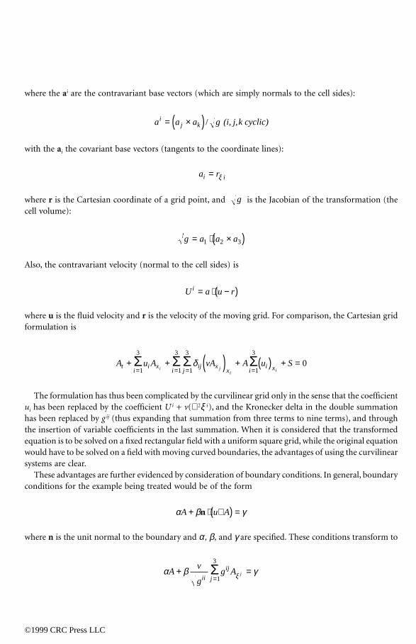
where the ai are the contravariant base vectors (which are simply normals to the cell sides):


with the ai the covariant base vectors (tangents to the coordinate lines):

where r is the Cartesian coordinate of a grid point, and is the Jacobian of the transformation (thecell volume):

Also, the contravariant velocity (normal to the cell sides) is

where u is the fluid velocity and r is the velocity of the moving grid. For comparison, the Cartesian gridformulation is

The formulation has thus been complicated by the curvilinear grid only in the sense that the coefficientui has been replaced by the coefficient U i + v(∇ 2ξ i), and the Kronecker delta in the double summationhas been replaced by g ij (thus expanding that summation from three terms to nine terms), and throughthe insertion of variable coefficients in the last summation. When it is considered that the transformedequation is to be solved on a fixed rectangular field with a uniform square grid, while the original equationwould have to be solved on a field with moving curved boundaries, the advantages of using the curvilinearsystems are clear.

These advantages are further evidenced by consideration of boundary conditions. In general, boundaryconditions for the example being treated would be of the form

where n is the unit normal to the boundary and α, β, and γ are specified. These conditions transform to

a a a gij k= ×( ) / (i, j,k cyclic)

a ri i= ξ

g

g a a a= ⋅ ×( )1 2 3

U a u ri = ⋅ −( )

A u A vA A u Sti

i xi j

ij xx i

i xi ji i

+ + ( ) + ( ) + == = = =Σ Σ Σ Σ

1

3

1

3

1

3

1

3

0δ

α β γA u A+ ⋅ ∇( ) =n

α β γξAv

gg A

ii j

ijj+ =

=Σ

1

3

for a boundary on which ξ i is constant. For comparison, the original boundary conditions can be writtenin the form


The transformed boundary conditions thus have the same form as the original conditions, but withthe coefficient nj replaced by g ij/ . The important simplification is the fact that the boundary to whichthe transformed conditions are applied is fixed and flat (coincident with a curvilinear coordinate surface).This permits a discrete representation of the derivative Aξ j along the transformed boundary without theneed for interpolation. By contrast, the derivative Axj in the original conditions cannot be discretizedalong the physical boundary without interpolation since the boundary is curved and may be in motion.

Although the transformed equation clearly contains more terms, the differencing is the same as on arectangular grid, i.e., it is done on the logically rectangular computational lattice, and the solution fieldis logically rectangular. Note that it is not necessary to discover and implement a transformation for eachnew boundary shape — rather the above formulation applies for all, simply with different values of (x,y, z) at the grid points.

The transformed PDE can also be expressed in conservative form as

for use in the finite volume approach. For more information on transformations, see Chapter 2.

P-3 Unstructured Grids

P-3.1 Connectivities and Data Structures

The basic difference between structured and unstructured grids lies in the form of the data structurewhich most appropriately describes the grid. A structured grid of quadrilaterals consists of a set ofcoordinates and connectivities that naturally map into elements of a matrix. Neighboring points in amesh in the physical space are the neighboring elements in the mesh matrix (Figure 14).

Thus, for example, a two-dimensional array x(i,j) can be used to store the x-coordinates of points ina 2D grid. The index i can be chosen to describe the position of points in one direction, while j describesthe position of points in the other direction. Hence, in this way, the indices i and j represent the twofamilies of curvilinear lines. These ideas naturally extend to three dimensions.

For an unstructured mesh the points cannot be represented in such a manner and additional infor-mation has to be provided. For any particular point, the connection with other points must be definedexplicitly in the connectivity matrix (Figure 15).

α β γA v n Ai

j x j+ =

=Σ

1

3

gii

gA g U A v g A gSt i

i

i

ijj

i

( ) + +

+ == =Σ Σ

1

3

1

3

0ξξ


A typical form of data format for an unstructured grid in two dimensions is

Number of Points,Number of Elements

x1, y1

x2, y2

x3, y3

…n1, n2, n3

n4, n5, n6

n7, n8, n9

…

where (x1, y1) are the coordinates of point i, and ni, 1=1,N are the point numbers with, for example, thetriad (n1, n2, n3) forming a triangle.

Other forms of connectivity matrices are equally valid, for example, connections can be based uponedges. The real advantage of the unstructured mesh is, however, because the points and connectivities

FIGURE 14

FIGURE 15

do not possess any global structure. It is possible, therefore, to add and delete nodes and elements as thegeometry requires or, in a flow adaptivity scheme, as flow gradients or errors evolve. Hence the unstruc-


tured approach is ideally suited for the discretization of complicated geometrical domains and complexflowfield features. However, the lack of any global directional features in an unstructured grid makes theapplication of line sweep solution algorithms more difficult to apply than on structured grids.

P-3.2 Grid Generation Approaches

In contrast to the generation of structured grids, algorithms to construct unstructured grids are frequentlybased upon geometrical ideas. There are now many techniques available, many of which are describedwithin this Handbook. For this elementary overview it is not appropriate to discuss details but tocomment on general procedures.

P-3.2.1 Triangle and Tetrahedra Creation by Delaunay Triangulation

The Delaunay approach to unstructured grid generation is now popular. The basic concepts go back asfar as Dirichlet, who in a paper in 1850 discussed the basic geometrical concept. Dirichlet proposed amethod whereby a given domain could be systematically decomposed into a set of packed convexpolygons. Given two points in the plane, P and Q, the perpendicular bisector of the line joining the twopoints subdivides the plane into two regions, V and W. The region V is closer to P than it is to Q.Extending these ideas, it is clear that for a given set of points in the plane, the regions Vi are territoriesthat can be assigned to each point so that Vi represents the space closer to Pi than to any other point inthe set. This geometrical construction of tiles is known as the Dirichlet tessellation. This tessellation ofa closed domain results in a set of non-overlapping convex polygons, called Voronoï regions, coveringthe entire domain.

From this description, it is apparent that in two dimensions, the territorial boundary that forms a sideof a Voronoï polygon must be midway between the two points it separates and is thus a segment of theperpendicular bisector of the line joining these two points. If all point pairs that have some segment ofa boundary in common are joined by straight lines, the result is a triangulation of the convex hull of theset of points Pi. This triangulation is known as the Delaunay triangulation.

Equivalent constructions can be defined in higher dimensions. In three dimensions, the territorialboundary that forms a face of a Voronoï polyhedron is equidistant between the two points it separates.If all point pairs that have a common face in the Voronoï construction are connected, then a set oftetrahedra is formed that covers the convex hull of the data points.

For the number of points which may be required in grid for computational analysis, it might appearthat the above procedure would be difficult and computationally expensive to construct. However, thereare several algorithms that can form the construction in a very efficient manner. These are discussed atlength in Chapters 1, 16 and 20. The approach is very flexible in that it can automatically create gridswith the minimum of user interaction for arbitrary geometries.

P-3.2.2 Triangle and Tetrahedra Creation by the Advancing Front Method

A grid generation technique based on the simultaneous point generation and connection is the advancingfront method. Unlike the Delaunay approach, advancing front methods are not based on any geometricalcriteria. They encompass the logical procedure of starting with a boundary grid of edges, in two dimen-sions, triangular faces, in three dimensions, and creating a point and constructing an element. Slowingthe initial boundary advances into the domain until the domain is filled with elements. The placing of

points within the domain is, like the Delaunay approach, controlled by a combination of a backgroundmesh and sources that provides the required data to ensure adequate resolution of the domain. The


algorithms that generate grids in this way are based on fast geometrical search routines. Details are tobe found in Chapter 17.

It is possible to combine techniques from both the Delaunay and the Advancing Front methods toproduce effective grid generation procedures – a sort of combination that tries to utilize the advantagesof both approaches. Chapter 18 discusses one such approach.

The Delaunay triangulation produces elements that are isotropic in nature. Although the AdvancingFront method can produce elements with stretching, it cannot produce high quality meshes with stretch-ing factors applicable to some problems, such as high Reynolds number viscous flows. Hence, it isnecessary to augment the standard procedures outlined above. In general, this is done by introducing amapping that ensures that regular isotropic grids can be generated but once mapped back to the physicalspace are distorted in a well defined manner to give appropriate element stretching. Such a method isdescribed in detail in Chapter 20.

P-3.2.3 Unstructured Grids of Quadrilaterals and Hexahedra

The preference of some developers for quadrilateral or hexahedral element based unstructured mesheshas resulted in effort devoted to the generation of such meshes. In two dimensions, it is possible tomodify the Advancing Front algorithm to construct quadrilaterals, although the additional complexityin extending this approach to three dimensions has not yet been overcome for practical geometries. Analternative approach that has seen some success is that of “paving.” This approach relies upon iterativelylayering or paving rows of elements in the interior of a region. As rows overlap or coincide they arecarefully connected together. It is fair to conclude that almost without exception the methods for theconstruction of unstructured hexahedral based grids are heuristic in nature, requiring considerable effortto include the many possible geometrical occurrences. Chapter 21 discusses in detail aspects of this kindof grid generation.

P-3.2.4 Surface Mesh Generation

The generation of unstructured grids on surfaces is, in itself, one of the most difficult and yet importantaspects of mesh generation in three dimensions. The surface mesh influences the field mesh close to theboundary. Surface meshes have the same requirement for smoothness and continuity as the field meshesfor which they act as boundary conditions, but in addition, they are required to conform to the geometrysurfaces, including lines of intersection and must accurately resolve regions of high curvature.

The approach usually taken to generate grids on surfaces is to represent the geometry in parametriccoordinates. A parametric representation of a surface is straightforward to construct and provides adescription of a surface in terms of two parametric coordinates. This is of particular importance, sincethe generation of a mesh on a surface then involves using grid generation techniques developed for twospace dimensions. A full description of these procedures is given in Chapter 19.

P-3.3 Grid Adaptation Techniques

To resolve features of a solution field accurately it is, in general, necessary to introduce grid adaptivitytechniques. Adaptivity is based on the equidistribution of errors principle, namely,

wi dsi = constant

where wi is the error or activity indicator at node i and dsi is the local grid point spacing at node i.Central to adaptivity techniques and the satisfaction of this equidistribution principle is to define an


appropriate indicator wi. Adaptivity criteria are based on an assessment of the error in the solution ofthe governing equations or are constructed to detect features of the field. These estimators are intimatelyconnected to the analysis equations to be solved. For example, some of the main features of a solutionof the Euler equations can be shock waves, stagnation points and vortices, and any indicator shouldaccurately identify these flow characteristics. However, for the Navier-Stokes equations, it is importantnot only to refine the mesh in order to capture these features but, in addition, to adequately resolveviscous dominated phenomena such as the boundary layers. Hence, it seems likely that, certainly in thenear future, adaptivity criteria will be a combination of measures, each dependent on some aspects ofthe flow and, in turn, on the flow equations.

There is also an extensive choice of criteria based on error analysis. Such measures include, a compar-ison of computational stencils of different orders of magnitude, comparison of the same derivatives ondifferent meshes, e.g., Richardson extrapolation, and resort to classical error estimation theory. Nogenerally applicable theory exists for errors associated with hyperbolic equations, hence, to date combi-nations of rather ad hoc methods have been used.

Once an adaptivity criterion has been established, the equidistribution principle is achieved througha variety of methods, including point enrichment, point derefinement, node movement and remeshing,or combinations of these. For more information on grid adaption techniques, see Chapter 35.

P-3.3.1 Grid Refinement

Grid refinement, or h-refinement, involves the addition of points into regions where adaptation isrequired. Such a procedure clearly provides additional resolution at the expense of increasing the numberof points in the computation.

Grid refinement on unstructured grids is readily implemented. The addition of a point or pointsinvolves a local reconnection of the elements, and the resulting grid has the same form as the initial grid.Hence, the same solver can be used on the enriched grid as was used on the initial grid.

It is important that the adaptivity criteria resolve both the discontinuous features of the solution (i.e.shock waves, contacts) and the smooth features as the number of grid points are increased. A desirablefeature of any adaptive method to ensure convergence is that the local cell size goes to zero in the limitof an infinite number of mesh points.

Grid refinement on a structured or multiblock grids is not so straightforward. The addition of pointswill, in general, break the regular array of points. The resulting distributed grid points no longer naturallyfit into the elements of an array. Furthermore, some points will not “conform” to the grid in that theyhave a different number of connections to other points. Hence grid refinement on structured gridsrequires a modification to the basic data structure and also the existence of so-called non-conformingnodes requires modifications to the solver. Clearly, point enrichment on structured grids is not as naturala process as the method applied on unstructured grids and hence is not so widely employed. Work hasbeen undertaken to implement point enrichment on structured grids and the results demonstrate thebenefits to be gained from the additional effort in modifications to the data structure and the solve.

P-3.3.2 Grid Movement

Grid movement satisfies the equidistribution principle through the migration of points from regions oflow activity into regions of high activity. The number of nodes in this case remains fixed. Traditionally,algorithms to move points involve some optimization principle. Typically, expressions for smoothness,

orthogonality and weighting according to the analysis field or errors are constructed and then an opti-mization is performed such that movement can be driven by a weight function, but not at the expense


of loss of smoothness and orthogonality. Such methods are in general, applicable to both structured andunstructured grids.

An alternative approach is to use a weighted Laplacian function. Such a formulation is often used tosmooth grids, and of course the formal version of the formulation is used as the elliptic grid generatorpresented earlier.

P-3.3.3 Combinations of Node Movement, Point Enrichment and Derefinement

An optimum approach to adaptation is to combine node movement and point enrichment with dere-finement. These procedures should be implemented in a dynamic way, i.e., applied at regular intervalswithin the simulation. Such an approach also provides the possibility of using movement and enrichmentto independently capture different features of the analysis.

P-3.3.4 Grid Remeshing

One method of adaptation which, to date, has been primarily used on unstructured grids, is adaptiveremeshing. As already indicated, unstructured meshes can be generated using the concept of a backgroundmesh. For an initial mesh, this is usually some very coarse triangulation that covers the domain and onwhich the spatial distribution is consistent with the given geometry. For adaptive remeshing, the solutionachieved on an initial mesh is used to define the local point spacing on the background mesh which wasitself the initial mesh used for the simulation. The mesh is regenerated using the new point spacing onthe background mesh. Such an approach can result in a second adapted mesh that contains fewer pointsthan that contained in the initial mesh. However, there is the overhead of regeneration of the mesh whichin three dimensions can be considerable. Nevertheless, impressive demonstrations of its use have beenpublished.

Contents


Foreword

Contributors

Acknowledgments

Preface: An Elementary Introduction Joe F. Thompson, Bharat K. Soni, and Nigel P. Weatherill

1 Fundamental Concepts and Approaches Joe F. Thompson and Nigel P. Weatherill

PART I Block-Structured Grids

Introduction to Structured Grids Joe F. Thompson

2 Mathematics of Space and Surface Grid Generation Zahir U.A. Warsi

3 Transfinite Interpolation (TFI) Generation Systems Robert E. Smith

4 Elliptic Generation Systems Stefan P. Spekreijse

5 Hyperbolic Methods for Surface and Field Grid GenerationWilliam M. Chan

6 Boundary Orthogonality in Elliptic Grid GenerationAhmed Khamayseh, Andrew Kuprat, and C. Wayne Mastin

7 Orthogonal Generation Systems Luís Eça

8 Harmonic Mappings Sergey A. Ivanenko

9 Surface Grid Generation Systems Ahmed Khamayseh and Andrew Kuprat

10 A New Approach to Automated Multiblock Decomposition for GridGeneration: A Hypercube++ Approach Sangkun Park and Kunwoo Lee

11 Composite Overset Structured Grids Robert L. Meakin


12 Parallel Multiblock Structured Grids Jochem Häuser, Peter R. Eiseman, Yang Xia, and Zheming Cheng

13 Block-Structured Applications Timothy Gatzke

PART II Unstructured Grids

Introduction to Unstructured Grids Nigel P. Weatherill

14 Data Structures for Unstructured Mesh Generation Luca Formaggia

15 Automatic Grid Generation Using Spatially Based TreesMark S. Shephard, Hugues L. de Cougny, Robert M. O’Bara, and Mark W. Beall

16 Delaunay–Voronoï Methods Timothy J. Baker

17 Advancing Front Grid Generation J. Peraire, J. Peiró, and K. Morgan

18 Unstructured Grid Generation Using Automatic Point Insertion and Local Reconnection David L. Marcum

19 Surface Grid Generation J. Peiró

20 Nonisotropic Grids Paul Louis George and Frédéric Hecht

21 Quadrilateral and Hexahedral Element Meshes Robert Schneiders

22 Adaptive Cartesian Mesh Generation Michael J. Aftosmis, Marsha J. Berger, and John E. Melton

23 Hybrid Grids Jonathon A. Shaw

24 Parallel Unstructured Grid Generation Hugues L. de Cougny and Mark S. Shephard

25 Hybrid Grids and Their Applications Yannis Kallinderis

26 Unstructured Grids: Procedures and Applications Nigel P. Weatherill

PART III Surface Definition


Introduction to Surface Definition Bharat K. Soni

27 Spline Geometry: A Numerical Analysis View David R. Ferguson

28 Computer-Aided Geometric Design Gerald Farin

29 Computer-Aided Geometric Design Techniques for Surface Grid Generation Bernd Hamann, Brian Jean, and Anshuman Razdan

30 NURBS in Structured Grid Generation Tzu-Yi Yu and Bharat K. Soni

31 NASA IGES And NASA-IGES NURBS Only Standard Austin L. Evans and David P. Miller

PART IV Adaptation and Quality

Introduction to Adaptation and Quality Bharat K. Soni

32 Truncation Error on Structured Grids C. Wayne Mastin

33 Grid Optimization Methods for Quality Improvement andAdaptation Olivier-Pierre Jacquotte

34 Dynamic Grid Adaptation and Grid Quality D. Scott McRae and Kelly R. Laflin

35 Grid Control and Adaptation O. Hassan and E. J. Probert

36 Variational Methods of Construction of Optimal Grids O. B. Khairullina, A. F. Sidorov, and O. V. Ushakova

37 Moving Grid Techniques Paul A. Zegeling

Appendix A: Grid Software and Configurations Bharat K. Soni

Appendix B: Grid Configurations Bharat K. Soni

©1999 crc press llc - freeebrary.free.fr/mesh generation/handbook_of_grid_ generation,1999... ·...

Documents