18. constrained optimization i: first order conditions

18. Constrained Optimization I: First

Order Conditions

The typical problem we face in economics involves optimization under constraints.From supply and demand alone we have: maximize utility, subject to a budget constraintand non-negativity constraints; minimize cost, subject to a quantity constraint; minimizeexpenditure, subject to a utility constraint; maximize profit, subject to constraints onproduction. And those are just the basic supply and demand related problems. Thenthere are other types of constrained optimization ranging from finding Pareto optimagiven resource and technology constraints to setting up incentive schemes subject toparticipation constraints.

The generic constrained optimization problem involves a thing to be optimized, theobjective function, and one or more constraint functions used to define the constraints.

It often looks something like this.

maxx

f(x)

s.t. gi(x) ≤ bi, for i = 1, . . . , k

hj(x) = cj, for j = 1, . . . , ℓ

Here f is the objective function, the equations gi(x) ≤ bi are referred to as inequalityconstraints, while the equations hj(x) = cj are called equality constraints.1

1 The letters “s.t.” can be read as “subject to”, “such that”, or “so that”.

2 MATH METHODS

18.1 Two Optimization Problems of Economics

Sometimes a problem will have only one kind of constraint. An example is the followingconsumer’s problem defining the indirect utility function v(p,m). It only has inequalityconstraints.

v(p,m) = maxx

u(x)

s.t. p·x ≤ m

x ≥ 0.

Here p is the price vector, u is the utility function, and m is income. All the constraintshere are inequality constraints. The constraints xi ≥ 0 (x ≥ 0) are known as non-negativity constraints. The solutions depend on the prices of consumer goods p andconsumer income m. We write the solution as x(p,m), and refer to them as theMarshallian demands.

Another example is the firm’s cost minimization problem which defines the costfunction c(w, q).

c(w, q) = minz

w·z

s.t. f(z) ≥ q, z ≥ 0.

Here q is the amount produced, w is the vector of factor prices, and f is the productionfunction. The solutions, now dependent on factor prices w and output q are theconditional factor demands, z(w, q).

18. CONSTRAINED OPTIMIZATION I: FIRST ORDER CONDITIONS 3

18.2 A Simple Consumer’s Problem

We start by examining a simple consumer’s problem with two goods and a singleequality constraint, the budget constraint. This consumer’s problem is

maxx

u(x1, x2)

s.t. p1x1 + p2x2 = m.

We’re dropping the usual non-negativity constraints in the interest of simplifying theproblem.

Consider the geometry of the solution. As we teach in undergrad micro, the indif-ference curve must be tangent to the budget line at the utility maximum. That is, theslopes of the two curves must be the same. This is illustrated in Figure 18.3.1. We haveextended the budget line because we are not imposing any non-negativity constraints.

u3

u2

u1

b x∗

x1

y1

Figure 18.2.1: Three indifference curves are shown in the diagram. Indifference curve u2

is the highest indifference curve the consumer can afford. This happens at x∗ where theindifference curve is tangent to the budget line.

4 MATH METHODS

18.3 Solution to the Simple Consumer’s Problems

Aligning the tangents for the budget line and indifference curve can be accomplishedby making sure they have the same slope. Both slopes are negative. The absolute slopeof the budget line is the relative price p1/p2 while the absolute slope of the indifferencecurve is the marginal rate of substitution, MRS12 = (∂u/∂x1)

/

(∂u/∂x2). It follows thatat the utility maximum x∗,

p1

p2=

∂u/∂x1

∂u/∂x2.

Another way to think about this is that we are lining up the tangent spaces of boththe budget constraint and the optimal indifference curve. Both the budget line and theindifference curves are level sets of functions. As such, their tangent spaces are the nullspaces of their derivatives.

The tangents v to the budget line obey (p1, p2)v = 0 and the tangents w to theoptimal indifference curve obey [Du(x∗)]w = 0. Since this is in R

2, the normal vectors∇u(x∗) and p = (p1, p2)T must be collinear. Thus ∇u(x∗) = µp for some µ ∈ R.

We could alternatively write the problem as maximizing u over the line −p·x = −m.It is the same set, but has a different derivative. We could use αp·x = αm for anyα 6= 0. Each α gives a different derivative to the constraint.

We don’t have the freedom to alter the direction of ∇u(x∗) because it points in thedirection of maximum increase of u. Reversing the direction would reverse consumerpreferences. What was better would become worse and vice-versa.

u2

bx∗

p

∇u(x∗)

p·x=m

u2

bx∗

−p

∇u(x∗)

−p·x

=−m

Figure 18.3.1: Here x∗ is the consumer’s utility maximum. At the maximum, the vectors pand ∇u(x∗) are collinear, with the heavier arrow being ∇u(x∗). With an equality constraint,it doesn’t matter whether the vectors point in the same or opposite directions. It will matterfor inequality constraints. The right panel writes the budget constraint as −p·x = −m. Eitherway, there is a µ ∈ R with ∇u(x∗) = µp.


18.4 More on the Simple Consumer’s Problem

If the tangents (or gradients) don’t align, the choice x∗ does not maximize utility. In thatcase there is a v with p·v = 0 and ∇u(x∗)·v > 0. Travelling along the tangent to thebudget constraint (the budget constraint itself) in the direction v will increase utility.

u3u2

bx∗

p′

∇u(x∗)

p′·x

=m

v

Figure 18.4.1: Here the prices have been changed to p′ so that the indifference curve andbudget line are no longer tangent. With the new prices, we can move along the budget linein the direction v to increase utility above u2 and even u3.

The situation is similar when x∗ is a minimum.The argument above is a key part of the proof of the upcoming Tangent Space

Theorem.

6 MATH METHODS

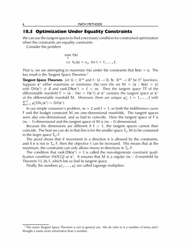
18.5 Optimization Under Equality Constraints

We can use the tangent spaces to find a necessary condition for constrained optimizationwhen the constraints are equality constraints.

Consider the problem

maxx

f(x)

s.t. hj(x) = cj, for i = 1, . . . , ℓ.

That is, we are attempting to maximize f(x) under the constraints that h(x) = c. Thekey result is the Tangent Space Theorem.2

Tangent Space Theorem. Let U ⊂ Rm and f : U → R, h : Rm → R

ℓ be C1 functions.Suppose x∗ either maximizes or minimizes f(x) over the set M = {x : h(x) = c}with Df(x∗) 6= 0 and rankDh(x∗) = ℓ < m. Then the tangent space TF of thedifferentiable manifold F = {x : f(x) = f(x∗)} at x∗ contains the tangent space at x∗

of the differentiable manifold M. Moreover, there are unique µ∗

j , i = 1, . . . , ℓ with∑ℓ

j=1 µ∗

jDhj(x∗) = Df(x∗).

In our simple consumer’s problem, m = 2 and ℓ = 1, so both the indifference curveF and the budget constraint M are one-dimensional manifolds. The tangent spaceswere also one-dimensional, and so had to coincide. Here the tangent space of F is(m− 1)-dimensional and the tangent space of M is (m− ℓ)-dimensional.

Because the dimensions are different if ℓ > 1, the tangent spaces cannot thencoincide. The best we can do in that line is for the smaller space Tx∗M to be containedin the larger space Tx∗F.

The proof shows that if movement in a direction v is allowed by the constraints,and if v is not in Tx∗F, then the objective f can be increased. This means that at themaximum, the constraints can only allows moves in directions in Tx∗F.

The condition that rankDh(x∗) = ℓ is called the non-degenerate constraint quali-fication condition (NDCQ) at x∗. It ensures that M is a regular (m − ℓ)-manifold byTheorem 15.26.1, which lets us find its tangent space.

Finally, the numbers µ∗

1, . . . , µ∗

ℓ are called Lagrange multipliers.

2 The name Tangent Space Theorem is not in general use. We do refer to it a number of times and Ithought a name more informative than a number.


18.6 Proof of the Tangent Space Theorem

Proof of Tangent Space Theorem. Suppose x∗ is a maximum. Because rankDh(x∗) =ℓ, there is a neighborhood U of x∗ where rankDh(x) = ℓ. By Theorem 15.26.1, wecan define a chart (U,ϕ) from U ∩ M to R

m−ℓ. It follows that the tangent spaceTx∗M = kerDh(x∗) is (m− ℓ)-dimensional.

Similarly, F is a (m − 1)-dimensional differentiable manifold, with an (m − 1)-dimensional tangent space Tx∗F.

By way of contradiction, suppose there is v ∈ Tx∗Mwith v /∈ Tx∗F. ThenDh(x∗)v =0 and Df(x∗)v 6= 0. The latter is a real number, so if Df(x∗)v < 0, we may replace vby −v, ensuring Df(x∗)v > 0.

Take a curve x(t) from (−1, 1) to M with x(0) = x∗ and x′(0) = v ∈ Tx∗M. This ispossible because the tangent space Tx∗M can also be defined as the set of tangents atx∗ of curves in M through x∗.

Use the continuity of Df(x) to pick ε > 0 so that Df(x)v > 0 for x ∈ Bε(x∗) ⊂ U∩M.By the Mean Value Theorem applied to φ(t) = f

(

x(t))

and the Chain Rule

f(

x(t))

= f(x∗) + Dfc(t)

(

x′(t))

for some c(t) ∈ ℓ(

x(t), x∗)

. For t small enough that x(t) ∈ Bε(x∗), we have

f(

x(t))

= f(x∗) + Dfc(t)v > f(x∗),

showing that x∗ is not a maximum, contradicting our hypothesis. This establishes thatTx∗M ⊂ Tx∗F.

Now for any pair of sets in Rm, A ⊂ B implies B⊥ ⊂ A⊥, where A⊥ denotes the

orthogonal complement, the set of vectors perpendicular to every vector in A.Applying this to the tangent spaces, we find (Tx∗F)⊥ ⊂ (Tx∗M)⊥. This impliesDf(x∗) ∈

(Tx∗M)⊥. Since Df is in the span of Dh, there are µ∗

j , j = 1, . . . , ℓ, with

Df(x∗) =ℓ∑

j=1

µ∗

jDhj(x∗).

Since rankDh(x∗) = ℓ, the Dhj are linearly independent, implying that the µ∗

j areunique.

8 MATH METHODS

18.7 The Lagrangian

The first order conditions for an optimum are usually written using the Lagrangian,

L(x,µ) = f(x) − µT(

h(x) − c)

= f(x) −ℓ∑

j=1

µj

(

hj(x) − cj)

.

This allows us to rewrite the key conclusions of the Tangent Space Theorem as follows:

Theorem 18.7.1. Let U ⊂ Rm and f : U → R, h : Rm → R

ℓ be C1 functions. Supposethat x∗ solves

maxx

f(x)

s.t. hj(x) = cj, for i = 1, . . . , ℓ

or

min x f(x)

s.t. hj(x) = cj, for i = 1, . . . , ℓ

and that rankDh(x∗) = ℓ holds, the non-degenerate constraint qualification (NDCQ).Then there are unique multipliers µ∗ such that (x∗,µ∗) is a critical point of the LagrangianL:

L(x,µ) = f(x) − µT(

h(x) − c)

.

That is,

∂L

∂xi(x∗,µ∗) = 0 for i = 1, . . . ,m

∂L

∂µj

(x∗,µ∗) = 0 for j = 1, . . . , ℓ.

Proof. If Df(x∗) 6= 0, this follows immediately from the Tangent Space Theorem.If Df(x∗) = 0, the fact that rankDh(x∗) = ℓ means that the ℓ rows of Dh are linearly

independent, so µ∗ = 0 is the unique vector with Df(x∗) = (µ∗)TDh(x∗).


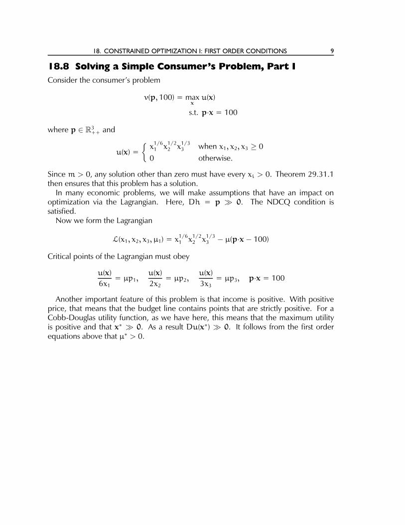
18.8 Solving a Simple Consumer’s Problem, Part I

Consider the consumer’s problem

v(p, 100) = maxx

u(x)

s.t. p·x = 100

where p ∈ R3++ and

u(x) =

{x

1/61 x

1/22 x

1/33 when x1, x2, x3 ≥ 0

0 otherwise.

Since m > 0, any solution other than zero must have every xi > 0. Theorem 29.31.1then ensures that this problem has a solution.

In many economic problems, we will make assumptions that have an impact onoptimization via the Lagrangian. Here, Dh = p ≫ 0. The NDCQ condition issatisfied.

Now we form the Lagrangian

L(x1, x2, x3, µ1) = x1/61 x

1/22 x

1/33 − µ(p·x− 100)

Critical points of the Lagrangian must obey

u(x)

6x1= µp1,

u(x)

2x2= µp2,

u(x)

3x3= µp3, p·x = 100

Another important feature of this problem is that income is positive. With positiveprice, that means that the budget line contains points that are strictly positive. For aCobb-Douglas utility function, as we have here, this means that the maximum utilityis positive and that x∗ ≫ 0. As a result Du(x∗) ≫ 0. It follows from the first orderequations above that µ∗ > 0.

10 MATH METHODS

18.9 Solving a Simple Consumer’s Problem, Part II

We can rewrite the first three equations by dividing them in pairs, eliminating both µand u(x). Thus

x2

3x1=

p1

p2,

x3

2x1=

p1

p3,

3x3

2x2=

p2

p3

The third equation is redundant, leaving us with

p2x2 = 3p1x1 and p3x3 = 2p1x1.

Substituting in our remaining equation, the budget constraint, we find

p·x = p1x1 + 3p1x1 + 2p1x1 = 6p1x1 = 100.

Then

x1 =100

6p1, x2 =

100

2p2, x3 =

100

3p3

This implies the indirect utility function is

v(p, 100) = u(x∗) =100

(6p1)1/6(2p2)1/2(3p3)1/3

The multiplier µ∗ is also easily calculated.

µ∗ =u(x∗)

100=

1

(6p1)1/6(2p2)1/2(3p3)1/3.

◭

How to Attack Such Problems. The basic steps used here were:

1. Rewrite the first order conditions as MRSij = pi/pj to eliminate the multiplierµ.

2. Express spending on each good in terms of spending on good one.3. Substitute into the budget constraint so that everything is in terms of good one.4. Solve for x1, then substitute back to solve for the other xj.

This often suffices to solve the problem, provided the equations involved are tractable.


18.10 Inequality Constraints: Binding or Not

Although our simple consumer’s problem in R2 involved only a single equality con-

straint, that is not typical. The consumer’s problem in R2 usually involves three in-

equality constraints—two non-negativity constraints and the budget constraint. Othereconomics problems, such as the firm’s cost minimization problem, or the consumer’sexpenditure minimization problem also use inequality constraints.

It will be helpful to distinguish cases where a particular constraint matters and whereit does not. We say that a constraint g(x) ≤ b binds at x∗ if g(x∗) = b. Otherwise theconstraint is non-binding.

12 MATH METHODS

18.11 A Single Inequality Constraint

Let’s start by investigating the case of a single inequality constraint. We will write themaximization problem in the following form:

maxx

u(x)

s.t. g(x) ≤ b

Figure 18.11.1 illustrates two possibilities that we need to consider. It shows that thesign of the multiplier matters when we have an inequality constraint. Both Du and Dgmust point in the same direction, otherwise we find ourselves minimizing utility overthe constraint set as in the right panel of Figure 18.11.1.

u1

u2

u3

g(x) ≤ b

b

x∗

∇g(x∗)

∇u(x∗)

u1

u2

u3

g(x) ≤ b

bx∗

∇g(x∗)

∇u(x∗)

Figure 18.11.1: Here x∗ is the consumer’s utility maximum with u(x∗) = u2. At themaximum, the vectors ∇g(x∗) and ∇u(x∗) are collinear, with the heavier arrow being ∇u(x∗).With an inequality constraint, like we have here, the two vectors must point in the samedirection. Then ∇u(x∗) = λ∇g(x∗) for some λ ≥ 0.

If ∇g(x∗) pointed in the opposite direction, it would mean that the region above u2 wouldhave lower values of g, as shown in the right panel. In that case utility is not maximized atx∗, since higher indifference curves such as u3 can be attained.

Another way to think about it is that when ∇u(x∗) = λ∇g(x∗), a small move inthe ∇u(x∗) direction will reduce g, and move into the interior of the constraint setwhile increasing utility. As in the proof of the Tangent Space Theorem, the Mean ValueTheorem can be used to show this.


18.12 Inequality Constraints: Complementary Slackness

The Tangent Space Theorem can be easily modified to ensure that the multiplier isnon-negative. However, there is another issue that might arise. The point x∗ could bein the interior of the constraint set, where g(x∗) < b. The Tangent Space Theorem doesnot apply there. However, x∗ is then an interior point, so Du(x∗) = 0.

This can be interpreted as the multiplier being zero, just as we did in the equalityconstraint case when Df(x∗) = 0.

There is a useful condition that lets up package this up using the Lagrangian frame-work. We impose the complementary slackness condition that

λ(

g(x) − b)

= 0.

If the constraint g(x) ≤ b binds, the complementary slackness condition tells us noth-ing. It’s already zero. If the constraint doesn’t bind, so g(x) − b < 0, it forces thecorresponding multiplier to be zero. This trick also works if we have several inequalityconstraints.

14 MATH METHODS

18.13 Maximization with Complementary Slackness

11/4/21

We sum up our discussion of complementary slackness in the following theorem.

Theorem 18.13.1. Let U ⊂ Rm and suppose f : U → R and g : U → R

k are C1

functions. Suppose that x∗ solves

maxx

f(x)

s.t. gi(x) ≤ bi.

and that k ≤ k constraints bind at x∗. Let g be the vector of functions defining thebinding inequality constraints at x∗ and b the corresponding constant terms. Form theLagrangian L:

L(x,λ) = f(x) − λT(

g(x) − b)

.

If rankDg(x∗) = k < m holds (NDCQ), then there are multipliers λ∗ such that

(a) The pair (x∗,λ∗) is a critical point of the Lagrangian:

∂L

∂xi(x∗,λ∗) = 0 for i = 1, . . . ,m

∂L

∂λj

(x∗,λ∗)hj(x∗) − cj = 0 for j = 1, . . . , k,

(b) The complementary slackness conditions hold:

λ∗

i

[

gi(x∗) − bi

]

= 0 for i = 1, . . . , k

(c) The multipliers are non-negative:

λ∗

1 ≥ 0, . . . , λ∗

k ≥ 0,

(d) The constraints are satisfied: g(x∗) ≤ b.


18.14 Failure of Constraint Qualification I

Now that we have a new tool, inequality constraints, you might be tempted to view anequality constraint as two inequality constraints. For example, you can write

p1x1 + p2x2 = m

as

p1x1 + p2x2 ≤ m

−p1x1 − p2x2 ≤ −m.

This doesn’t work. It runs afoul of the NDCQ. When both bind, as they must if bothare obeyed, we have

Dg =(

p1 p2

−p1 −p2

)

.

This has rank 1 when it needs rank 2. In this case, the failure of constraint qualificationis minor. If you do this with Cobb-Douglas utility, you won’t be able to uniquelydetermine the two multipliers. However, you can determine their difference.

16 MATH METHODS

18.15 Solving a Cobb-Douglas Consumer’s Problem I

The key to understanding how to use Theorem 18.13.1 is that complementary slack-ness conditions are a way of checking all the possible cases where some, but not all,constraints bind. Let’s look at a concrete problem in R

2 to see how this works.

maxx

x1/31 x

2/32

s.t. p1x1 + p2x2 ≤ m

x1 ≥ 0, x2 ≥ 0.

Where p1, p2,m > 0.We form the Lagrangian by first rewriting the non-negativity constraints in the proper

form: −x1 ≤ 0, −x2 ≤ 0. The Lagrangian is

L = u(x) − λ0(p1x1 + p2x2 −m) − λ1(−x1) − λ2(−x2)

= u(x) − λ0(p1x1 + p2x2 −m) + λ1x1 + λ2x2.

Non-negativity constraints always yield terms of the form +λixi.


18.16 Solving a Cobb-Douglas Consumer’s Problem II

We now turn to constraint qualification. Consider

Dg =

(

p1 p2

−1 00 −1

)

Now if only constraint i binds, we must have Dgi(x∗) 6= 0, and we do. If twoconstraints bind, the matrix Dg(x∗) obtained by deleting the non-binding row must beinvertible, which it is. It is not possible for all three constraints to bind at once as wewould have p1(0) + p2(0) = m > 0. The NDCQ condition is satisfied.

p1x1 + p2x2 < m

x1 = 0 & p·x = m

x2 = 0 & p·x = mx1 = 0 & x2 = 0

b

bx2 = 0

x1

=0

p1 x

1 +p2 x

2 =m

x1

x2

Figure 18.16.1: Without complementary slackness, we would have to check separately formaxima eight ways: at each of the three corner points, in the relative interior of each of thethree boundary segments of the budget set, and in the interior of the budget set.

18 MATH METHODS

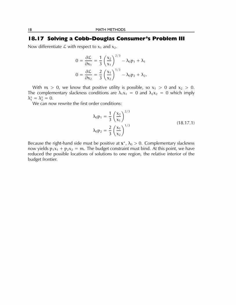
18.17 Solving a Cobb-Douglas Consumer’s Problem III

Now differentiate L with respect to x1 and x2.

0 =∂L

∂x1=

1

3

(

x2

x1

)2/3

− λ0p1 + λ1

0 =∂L

∂x2=

2

3

(

x1

x2

)1/3

− λ0p2 + λ2.

With m > 0, we know that positive utility is possible, so x1 > 0 and x2 > 0.The complementary slackness conditions are λ1x1 = 0 and λ2x2 = 0 which implyλ∗

1 = λ∗

2 = 0.We can now rewrite the first order conditions:

λ0p1 =1

3

(

x2

x1

)2/3

λ0p2 =2

3

(

x1

x2

)1/3(18.17.1)

Because the right-hand side must be positive at x∗, λ0 > 0. Complementary slacknessnow yields p1x1 + p2x2 = m. The budget constraint must bind. At this point, we havereduced the possible locations of solutions to one region, the relative interior of thebudget frontier.


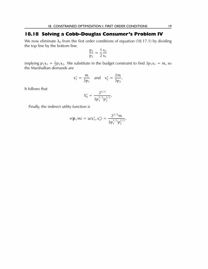
18.18 Solving a Cobb-Douglas Consumer’s Problem IV

We now eliminate λ0 from the first order conditions of equation (18.17.1) by dividingthe top line by the bottom line.

p1

p2=

1

2

x2

x1

implying p1x1 = 12p2x2. We substitute in the budget constraint to find 3p1x1 = m, so

the Marshallian demands are

x∗1 =m

3p1and x∗2 =

2m

3p2.

It follows that

λ∗

0 =22/3

3p1/31 p

2/32

.

Finally, the indirect utility function is

v(p,m) = u(x∗1, x∗

2) =22/3m

3p1/31 p

2/32

.

20 MATH METHODS

18.19 Complementary Slackness Gone Wild: I

Let’s try to maximize a linear utility function in R3+. One thing that’s different about

this problem is that it is purely an exercise in the use of complementary slackness.The problem is:

maxx

u(x) = a1x1 + a2x2 + a3x3

s.t. p1x1 + p2x2 + p3x3 ≤ m

x1 ≥ 0, x2 ≥ 0, x3 ≥ 0.

Where p ≫ 0, m > 0, and each ai > 0. Theorem 29.31.1 guarantees that the problemhas a solution.

We next check constraint qualification. Here

Dg =

p1 p2 p3

−1 0 00 −1 00 0 −1

.

It is impossible for all four constraints to bind. If they did, we would have x1 = x2 =x3 = 0 and 0 = p·x = m > 0. Any collection of 1, 2, or 3 rows of Dg is linearlyindependent, so constraint qualification (NDCQ) is satisfied.


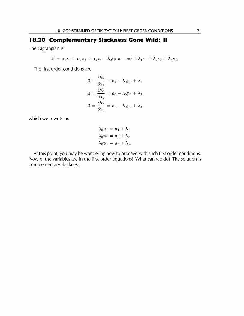
18.20 Complementary Slackness Gone Wild: II

The Lagrangian is

L = a1x1 + a2x2 + a3x3 − λ0(p·x−m) + λ1x1 + λ2x2 + λ3x3.

The first order conditions are

0 =∂L

∂x1= a1 − λ0p1 + λ1

0 =∂L

∂x2= a2 − λ0p2 + λ2

0 =∂L

∂x3= a3 − λ0p3 + λ3

which we rewrite as

λ0p1 = a1 + λ1

λ0p2 = a2 + λ2

λ0p3 = a3 + λ3.

At this point, you may be wondering how to proceed with such first order conditions.Now of the variables are in the first order equations! What can we do? The solution iscomplementary slackness.

22 MATH METHODS

18.21 Complementary Slackness Gone Wild: III

To recapitulate, we have the following first order conditions:

λ0p1 = a1 + λ1

λ0p2 = a2 + λ2

λ0p3 = a3 + λ3.

(18.21.2)

Now λ1 ≥ 0, so λ0p0 ≥ a1 > 0. This implies λ0 > 0. Complementary slacknesstells us that λ0(p·x−m) = 0. Since λ0 > 0, that means p·x = m > 0. The consumerspends their entire budget.

Dividing each line of equation (18.21.2) by pi tells us

λ0 = a1/p1 + λ1/p1 ≥ a1/p1

λ0 = a2/p2 + λ2/p2 ≥ a2/p2

λ0 = a3/p3 + λ3/p3 ≥ a3/p3.

(18.21.3)

Thenλ0 ≥ max

i=1,2,3{ai/pi}.

If λ0 > maxi=1,2,3{ai/pi}, then each λi > 0 for i = 1, 2, 3. Complementary slacknessrequires that λixi = 0 for i = 1, 2, 3, implying that x1 = x2 = x3 = 0. But this isimpossible because we know p·x = m > 0. At least one xi must be positive, and forthat i, λ0 = ai/pi. So we can write

λ0 = maxi=1,2,3

{ai

pi

}

.


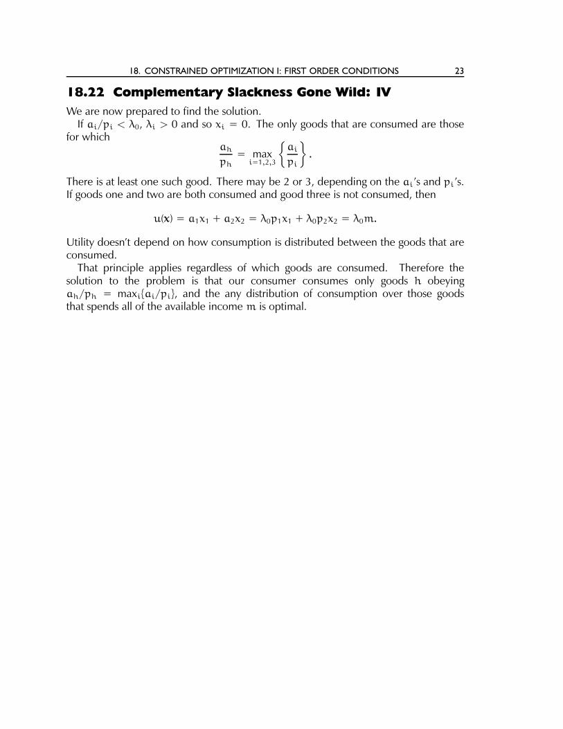
18.22 Complementary Slackness Gone Wild: IV

We are now prepared to find the solution.If ai/pi < λ0, λi > 0 and so xi = 0. The only goods that are consumed are those

for whichah

ph

= maxi=1,2,3

{ai

pi

}

.

There is at least one such good. There may be 2 or 3, depending on the ai’s and pi’s.If goods one and two are both consumed and good three is not consumed, then

u(x) = a1x1 + a2x2 = λ0p1x1 + λ0p2x2 = λ0m.

Utility doesn’t depend on how consumption is distributed between the goods that areconsumed.

That principle applies regardless of which goods are consumed. Therefore thesolution to the problem is that our consumer consumes only goods h obeyingah/ph = maxi{ai/pi}, and the any distribution of consumption over those goodsthat spends all of the available income m is optimal.

24 MATH METHODS

18.23 Example: Quasi-linear Utility I SKIPPED

Now consider maximizing the quasi-linear utility function u(x, y) = x +√y. We

must solve:

maxx

u(x) = x +√y

s.t. pxx + pyy ≤ m

x ≥ 0, y ≥ 0.

As in the last two problems, anxd most standard consumer’s problems, the NDCQcondition is satisfied. The Lagrangian is

L = x +√y− λ0(pxx + pyy−m) + λxx + λyy

yielding first order conditions

0 =∂L

∂x= 1 − λ0px + λx

0 =∂L

∂y= − 1

2√y

+ λy.(18.23.4)


18.24 Example: Quasi-linear Utility II SKIPPED

We rewrite equation (18.23.4) as

λ0px = 1 + λx

λ0py =1

2√y

+ λy.(18.24.5)

The top line of equation (18.24.5) implies λ0 ≥ 1/px > 0. By complementaryslackness, the budget constraint must bind: pxx + pyy = m. This is also the usualresult in standard consumer’s problems.

There are now three cases to consider, depending on which constraints bind. Weorganize these based on the variables. This is usually better than trying to organizebased on the multipliers because when a multiplier is zero, that constraint may stillbind. The values of the multipliers do not translate nicely into information about whichconstraints bind.

The cases are (I) x > 0 and y = 0, (II) x = 0 and y > 0, and (III) x > 0 and y > 0.By using complementary slackness, we have reduced the original eight cases to three.

26 MATH METHODS

18.25 Example: Quasi-linear Utility III SKIPPED

Our first order conditions are

λ0px = 1 + λx

λ0py =1

2√y

+ λy.(18.24.5)

Case I: Here x > 0 and y = 0. The complementary slackness condition λxx = 0tells us that λx = 0. By the top line of equation (18.24.5), λ0 = 1/px. The secondequation of equation (18.24.5) becomes

py/px =1

2√y

+ λy.

But this is impossible to satisfy since y = 0. Case I is out.Case II: Here x = 0 and y > 0. The complementary slackness condition λyy = 0

implies λy = 0, so the bottom line of equation (18.24.5) becomes

λ0py =1

2√y

The budget constraint tells us y = m/py. It follows that λ0 = 1/2√pym. By the top

line of equation (18.24.5),px

2√pym

= 1 + λx ≥ 1.

This solution works if p2x ≥ 4pym.


18.26 Example: Quasi-linear Utility IV SKIPPED

Case III: Here x, y > 0. By complementary slackness λx = λy = 0, so the first orderconditions (18.24.5) are

λ0px = 1

λ0py =1

2√y.

Then λ0 = 1/px and py/px = 1/2√y. It follows that y = p2

x/4p2y. Using the budget

constraint, we find pxx = m− pyy = m− p2x/4py. The non-negativity constraint for

x requires m− p2x/4py ≥ 0 or equivalently, 4pym ≥ p2

x.Collecting the results together, we find

(x, y) =

(

0, mpy

)

when p2x ≥ 4pym

(

mpx

− px

4p2y

, p2x

4py

)

when p2x ≤ 4pym.

When p2x = 4pym, the two cases agree.

28 MATH METHODS

18.27 Failure of Constraint Qualification II

In some cases, the failure of constraint qualification is quite serious, serious enough thatit prevents us from solving the problem as advertised. Consider this example borrowedfrom section 19.5 of Simon and Blume.

max(x,y)

x

s.t. x3 + y2 = 0.

Suppose we blindly charge ahead, setting up the Lagrangian

L = x− µ(x3 + y2).

The critical points of the Lagrangian solve

1 = 3µx2, 0 = 2µy, and x3 + y2 = 0.

There are no solutions. If y = 0, x = 0 by the constraint, so 1 = 3µx2 = 0, which isimpossible. If µ = 0, we again have 1 = 0, another impossibility. But 0 = 2µy so oneof µ or y must be zero, but neither can be zero. Our method has failed!


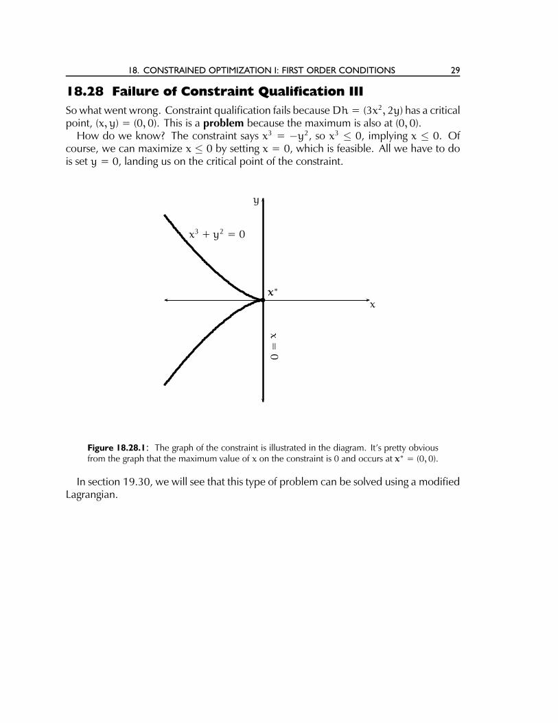
18.28 Failure of Constraint Qualification III

So what went wrong. Constraint qualification fails because Dh = (3x2, 2y) has a criticalpoint, (x, y) = (0, 0). This is a problem because the maximum is also at (0, 0).

How do we know? The constraint says x3 = −y2, so x3 ≤ 0, implying x ≤ 0. Ofcourse, we can maximize x ≤ 0 by setting x = 0, which is feasible. All we have to dois set y = 0, landing us on the critical point of the constraint.

x3 + y2 = 0

x=

0bx∗

x

y

Figure 18.28.1: The graph of the constraint is illustrated in the diagram. It’s pretty obviousfrom the graph that the maximum value of x on the constraint is 0 and occurs at x∗ = (0, 0).

In section 19.30, we will see that this type of problem can be solved using a modifiedLagrangian.

30 MATH METHODS

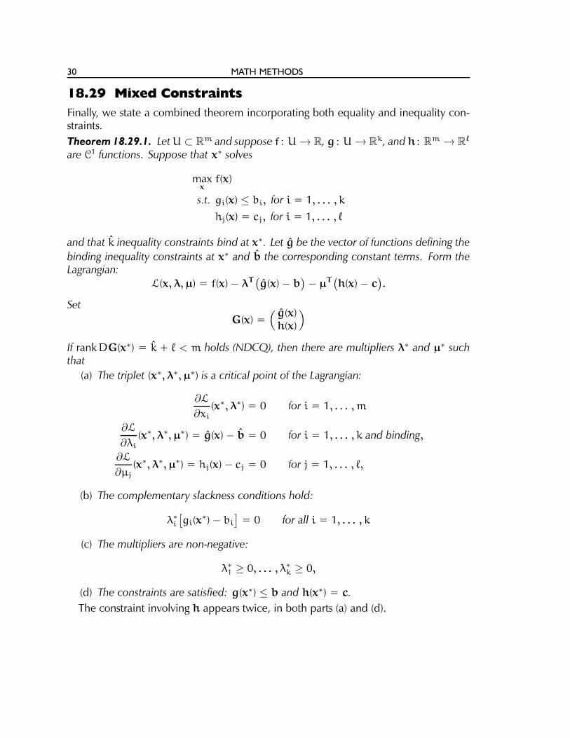
18.29 Mixed Constraints

Finally, we state a combined theorem incorporating both equality and inequality con-straints.

Theorem 18.29.1. LetU ⊂ Rm and suppose f : U → R, g : U → R

k, and h : Rm → Rℓ

are C1 functions. Suppose that x∗ solves

maxx

f(x)

s.t. gi(x) ≤ bi, for i = 1, . . . , k

hj(x) = cj, for i = 1, . . . , ℓ

and that k inequality constraints bind at x∗. Let g be the vector of functions defining the

binding inequality constraints at x∗ and b the corresponding constant terms. Form theLagrangian:

L(x,λ,µ) = f(x) − λT(

g(x) − b)

− µT(

h(x) − c)

.

Set

G(x) =(

g(x)h(x)

)

If rankDG(x∗) = k + ℓ < m holds (NDCQ), then there are multipliers λ∗ and µ∗ suchthat

(a) The triplet (x∗,λ∗,µ∗) is a critical point of the Lagrangian:

∂L

∂xi(x∗,λ∗) = 0 for i = 1, . . . ,m

∂L

∂λi

(x∗,λ∗,µ∗) = g(x) − b = 0 for i = 1, . . . , k and binding,

∂L

∂µj

(x∗,λ∗,µ∗) = hj(x) − cj = 0 for j = 1, . . . , ℓ,


λ∗

i

[

gi(x∗) − bi

]

= 0 for all i = 1, . . . , k


λ∗

1 ≥ 0, . . . , λ∗

k ≥ 0,

(d) The constraints are satisfied: g(x∗) ≤ b and h(x∗) = c.

The constraint involving h appears twice, in both parts (a) and (d).


18.30 Example with Mixed Constraints I

Consider the problem

maxx

f(x, y) = x2 − y2

s.t. x ≥ 0, y ≥ 0

x2 + y2 = 4.

The constraint set is compact, and the function is continuous, so it will have bothmaxima and minima by the Weierstrass Theorem.

The matrix Dg will be a submatrix of

( 2x 2y−1 00 −1

)

.

Any 2×2 submatrix of this has rank 2 and all rows are non-negative because x2 +y2 = 4and x, y ≥ 0. Finally, it is impossible for all three constraints to bind, implying the NDCQcondition is satisfied.

Form the Lagrangian

L = x2 − y2 − µ(x2 + y2 − 4) + λxx + λyy.

The first order conditions are

0 =∂L

∂x= 2x− 2xµ + λx

0 =∂L

∂y= −2y− 2yµ + λy

0 =∂L

∂µ= −x2 − y2 + 4

The last one is the equality constraint. The solution must also obey the two comple-mentary slackness conditions

λxx = 0, λyy = 0

and the non-negativity constraints

x ≥ 0, y ≥ 0, λ ≥ 0.

32 MATH METHODS

18.31 Example with Mixed Constraints II

We rewrite the first order conditions

2x + λx = 2µx

2y + 2µy = λy

Multiply the first equation by x and the second by y, obtaining

2x2 + λxx = 2µx2

2y2 + 2µy2 = λyy

Apply complementary slackness to both: λxx = 0 and λyy = 0. Then

2x2 = 2µx2

2y2 + 2µy2 = 0.

From the first equation, if x > 0 then µ = 1, while according to the second equation,if y > 0, µ = −1. At least one of x and y must be zero. They can’t both be zero dueto the constraint x2 + y2 = 4.

That gives us two cases to consider: (1) x > 0, y = 0, and (2) y > 0, x = 0.Case I: x > 0 and y = 0. Here µ = +1, λx = 0 and λy = 0. Since x2 + y2 = 4 and

x ≥ 0, this solution is (2, 0) with f(2, 0) = 4.Case II: x = 0 and y > 0. Here µ = −1, λx = 0 and λy = 0. Since x2 + y2 = 4

and y ≥ 0, this solution is (0, 2) with f(0, 2) = −4.Based on these results, (2, 0) is the maximum point and (0, 2) is the minimum point.


18.32 Minimization with Inequality Constraints

When we only had equality constraints, the same conditions found critical points forboth maxima and minima. That is no longer true when there are inequality constraintsas the sign of the associated multipliers depends on whether we are maximizing orminimizing.

There are various ways to handle minimization problems with inequality constraints.One of the more obvious is to maximize −f instead of minimizing f. That yieldsLagrangian

L(x,λ,µ) = −f(x) − λT(

g(x) − b)

− µT(

h(x) − c)

.

Multiplying by −1, we obtain

f(x) + λT(

g(x) − b)

+ µT(

h(x) − c)

.

Since the sign of µ doesn’t matter, this is equivalent to using the Lagrangian

L1(x,λ,µ) = f(x) + λT(

g(x) − b)

− µT(

h(x) − c)

.

where λ ≥ 0 or using

L2(x,λ,µ) = f(x) − λT(

g(x) − b)

− µT(

h(x) − c)

.

with λ ≤ 0. Yet another method is the one favored in the book, writing the inequalityconstraints the opposite way, setting g′ = −g and b′ = −b, yielding constraintsg′(x) ≥ b′ instead of g(x) ≤ b. We will state the result in this form, which is morenatural when thinking about duality.

It doesn’t really matter which form of Lagrangian you use. Just be sure not to mixthem!

34 MATH METHODS

18.33 Minimization with Mixed Constraints

We state a version Theorem 18.29.1 that works for minimization problems.

Theorem 18.33.1. LetU ⊂ Rm and suppose f : U → R, g : U → R

k, and h : Rm → Rℓ

are C1 functions. Suppose that x∗ solves

minx

f(x)

s.t. gi(x) ≥ bi, for i = 1, . . . , k

hj(x) = cj, for i = 1, . . . , ℓ

and that k constraints bind at x∗. Let g be the vector of binding inequality constraints at

x∗ and b the corresponding constants. Form the Lagrangian L:

L(x,λ,µ) = f(x) − λT(

g(x) − b)

− µT(

h(x) − c)

.

If

rankD(

g(x∗)h(x∗)

)

= k + ℓ < m

holds (NDCQ), then there are multipliers λ∗ and µ∗ such that

(a) The triplet (x∗,λ∗,µ∗) is a critical point of the Lagrangian:

∂L

∂xi(x∗,λ∗) = 0 for i = 1, . . . ,m

∂L

∂λi

(x∗,λ∗,µ∗) = gi(x) − bi = 0 for binding i = 1, . . . , k,

∂L

∂µj

(x∗,λ∗,µ∗) = hj(x∗) − cj = 0 for j = 1, . . . , ℓ,


λ∗

i

[

gi(x∗) − bi

]

= 0 for all i = 1, . . . , k


λ∗

1 ≥ 0, . . . , λ∗

k ≥ 0,

(d) The constraints are satisfied: g(x∗) ≥ b and h(x∗) = c.

November 14, 2021

Copyright c©2021 by John H. Boyd III: Department of Economics, Florida InternationalUniversity, Miami, FL 33199

18. constrained optimization i: first order conditions

Documents