M. Pettini: Introduction to Cosmology — Lecture 17

THE COSMIC DISTANCE LADDER

17.1 Introduction

In 1929, the Carnegie astronomer Edwin Hubble, working with data ob-tained at the Mount Wilson Observatory in California, published the firstplot showing that galaxies are receding from us with a radial velocity pro-portional to their distance. The logical conclusion is that our Universe is ina state of expansion, and Hubble’s discovery stands as one of the most pro-found of the twentieth century. This result had been anticipated two yearsearlier by Lemaıtre, who found a mathematical solution for an expandinguniverse and noted that it provided a natural explanation for the observedreceding velocities of galaxies. His results were published (in French) inthe Annals of the Scientific Society of Brussels and were not widely knownuntil 1931 when they were highlighted by Eddington.

As can be appreciated from inspection of Figure 17.1, the slope of the orig-inal ‘Hubble diagram’ implies a value of the Hubble constant, H0 = v/dwhich is one order of magnitude greater than the value generally acceptedtoday, H0 ' 70 km s−1 Mpc−1 with an uncertainty of about 10%. While itis relatively straightforward to measure the recession velocities of galaxies

Figure 17.1: The original Hubble diagram, reproduced from Freedman & Madore 2010,ARAA, 48, 673.

1

from the redshifts of emission and/or absorption lines in their spectra, thedetermination of distances to astronomical objects is fraught with difficul-ties and plagued by systematic uncertainties.

Indeed, the history of the determination of the Hubble constant does notshow astronomers in a good light: for decades there were two ‘camps’, oneclaiming H0 = 50 km s−1 Mpc−1 and the other double that value; bothgroups estimated their error to be about 10% and were generally unwillingto concede that systematic uncertainties could significantly inflate theirerror estimates. The issue was finally resolved in the mid-1990s, largelythanks to observations performed with the Hubble Space Telescope. Giventhe central importance of an accurate measure of the Hubble constant forthe whole of cosmology, you will not be surprised to learn that this was oneof the original scientific motivations for building the Hubble Space Telescopeand that a great deal of observing time was devoted to this ‘Key Project’in the first few years of operation of HST.

Measuring the Hubble constant requires constructing what is referred to a‘cosmic distance ladder’. Distances to objects at cosmological distances areestablished step by step, identifying classes of astronomical sources who actas ‘standard candles’ over ever increasing distances. The calibration of one

Figure 17.2: The cosmic distance ladder.

2

class of sources at nearby distances, for example a particular type of star, isused to calibrate the intrinsic luminosity of another type of source, whichbeing intrinsically more luminous (but also rarer), can then be followedto larger distances, and so on. Clearly systematic errors can build veryquickly!

In general terms, to measure H0 distance measurements must be obtainedfar enough away to probe the smooth Hubble expansion (that is, at suffi-ciently large distances that the random velocities induced by gravitationalinteractions with neighboring galaxies are small relative to the Hubblevelocity), and nearby enough to calibrate the absolute, not simply the rel-ative, distance scale. The objects under study also need to be sufficientlyabundant that their statistical uncertainties do not dominate the errorbudget. Ideally the method should have a solid physical underpinning andhigh internal accuracy, amenable to empirical tests for systematic errors.

Over the years, many classes of astronomical sources have been exploredwith a view to establishing their suitability as standard candles (see Fig-ure 17.2). Here we shall briefly review some of the main ones.

17.2 Cepheids

Chepeids are the first rung in the extragalactic distance ladder and hold aspecial place in the subject because they were used by Hubble in his firstradial velocity vs. distance plot that led to the discovery of the expandingUniverse. Cepheids are a class of variable stars located in the upper H-R di-agram (see Figure 17.3); they are evolved, core helium-burning stars whoseprogenitors are thought to have been B- or late O-type main sequence stars.Their visual magnitudes vary in a regular fashion with amplitudes of be-tween a few tenths of magnitude and ∼ 2 magnitudes, with periods rangingfrom a few days to a few weeks (see right-hand panel of Figure 17.3).

The key role that Cepheids have played in the determination of the extra-galactic distance scale stems from the existence of a tight period-luminosityrelation: the longer the period of their variability, the brighter their ab-solute magnitude. Cepheids are supergiant stars with R ∼ 50 R andL >∼ 103 L, bright enough to be seen over intergalactic distances. Thus,by measuring the period of an extragalactic Cepheid star, it is possible to

3

deduce its distance modulus by comparing its observed magnitude withthe absolute magnitude, provided the period-luminosity relationship hasbeen calibrated with the known distances of nearby Cepheids in the MilkyWay. A later refinement of the calibration includes a colour term, givingthe period-luminosity-colour (PLC) relation:

MV = α logP + β(B − V )0 + γ

where α is a negative number and (B − V )0 is the intrinsic B − V colourobtained after correcting for interstellar extinction.

Cepheids stars undergo periodic radial pulsations that are at the root of thePLC relation via Stephan’s law: L = 4πR2σT 4. The change in luminosityis driven primarily by changes in surface temperature, while the period isrelated to the stellar radius via the mean density (for mechanical systemsit is well known that Pρ1/2 = Q, where Q is a structural constant).

Cepheid pulsation occurs because of the changing atmospheric opacity withtemperature in the helium ionization zone (the zone where He transitionsfrom He+ to He2+). This zone acts like a heat engine and valve mecha-nism. During the portion of the cycle when the ionization layer is opaqueto radiation, that layer traps energy, resulting in an increase in its internalpressure. This added pressure acts to elevate the layers of gas above it,

Figure 17.3: Left: Locations of different types of variable stars in the H-R diagram. Left:Light curve of δ Cephei, the prototype of the Cepheid variable stars.

4

resulting in the observed radial expansion. As the star expands, it doeswork against gravity and the gas cools. As it does so, its temperaturefalls back to a point where the doubly ionized helium layer recombines andbecomes transparent again, thereby allowing more radiation to pass. With-out that added source of heating the local pressure drops, the expansionstops, the star recollapses, and the cycle repeats. The alternate trappingand releasing of energy in the helium ionization layer ultimately gives riseto the periodic change in radius, temperature, and luminosity seen at thesurface. Not all stars are unstable to this mechanism. The cool (red) edgeof the Cepheid instability strip is thought to be controlled by the onsetof convection, which then prevents the helium ionization zone from driv-ing the pulsation. For hotter temperatures, the helium ionization zone islocated too far out in the atmosphere for significant pulsations to occur.

There are complications, of course. Stars spend only a short fraction oftheir lives in the so-called ‘instability strip’ of the H-R diagram. Therefore,Cepheids are relatively rare and we have to go a long way from the Sunbefore we encounter one. Consequently, there are just ten Cepheids withaccurately measured trigonometric parallaxes.1 The resulting error in theCepheid zero point is ±0.06 mag ( ±3%). This error will be reduced con-siderably when data from the on-going Global Astrometric Interferometerfor Astrophysics (GAIA) mission are gathered and analysed.

Further complications are: interstellar reddening, which can be mitigatedby observations at infrared wavelengths; crowding of stellar images (this iswhere HST played a key role with its superior spatial resolution); and thedependence of the PLC relation on the metallicity of the stars. Concerningthis last point, it should be clear from your Stellar Structure and Evolutioncourse that metallicity has an impact on the opacity of stellar layers. Sinceit is changes in opacity that drive stellar pulsations, it is reasonable toexpect that there will be a metallicity dependence of the PLC relation.However, predicting the magnitude (and even simply the sign of the effect)at either optical or infrared wavelengths, has proved challenging. Differenttheoretical and empirical studies have led to a range of conclusions, andthe effect of metallicity on the observed properties of Cepheids is still anactive and on-going area of research.

1Other methods to calibrate the Cepheid zero point have been proposed, but none is as reliable asaccurately measured parallaxes.

5

17.3 The Distance to the Large Magellanic Cloud

The next rung in the cosmic distance ladder, and the first one outside theMilky Way, is our nearest companion galaxy, the Large Magellanic Cloud(LMC). Given its importance as a stepping stone to extragalactic distancesand its proximity to our Galaxy, there have been numerous attempts atmeasuring the distance to the LMC.

One of the most direct uses the light echoes of SN 1987A, the closest su-pernova since the invention of the telescope. Approximately 240 days afterthe supernova explosion, a ring of circumstellar material, ejected duringan earlier phase in the evolution of the supernova progenitor, became vis-ible as the flash of UV radiation accompanying the SN explosion reachedit and ionised it. (This is the inner ring in Figure 17.4; the origin of thetwo outer rings is still unclear.) For the inner ring, we know its physicalradius, R = c∆t with ∆t = 240 days, and its angular radius on the sky,θ = 0.85 arcsec,2 and we can therefore solve for the distance to the SN:

DLMC =c∆t

θ= 1.51× 1023 cm = 48.9 kpc

which corresponds to a distance modulus (m−M)LMC = 18.45.2The ring is actually inclined to our line of sight which is why we see it as an ellipse, but this geometric

effect can be accounted for.

Figure 17.4: Images of SN1987A and its immediate surroundings recorded with the HubbleSpace Telescope on 6 February 1996 (Left) and 6 December 2006 (Right). The inner ringhas been brightening in clumps as the shock front from the supernova began collidingwith the slower moving material ejected by the SN progenitor during its red supergiantphase.

6

Figure 17.5: Probability distributions of 180 distance modulus estimates to the LMC.Individual estimates are shown by unit-area Gaussians with a dispersion set to theirquoted statistical errors (thick blue lines). The thin solid purple line represents therenormalized sum of those Gaussians. The thick broken red line represents the value(m−M) = 18.39 mag with a systematic error of ±0.03 mag based on the Galactic paral-lax calibration of Cepheids (see Section 17.2) and corrected for the LMC metallicity by−0.05 mag. The circled dot with error bar shows the median value of the non-Cepheiddistance determinations. Note that a distance modulus m −M = 18.40 corresponds toa distance of 47.9 kpc. (Figure reproduced from Freedman & Madore 2010, ARAA, 48,673).

Several thousand Cepheids have been identified and cataloged in the LMC,all at essentially the same distance. As can be seen from Figure 17.5,the calibration of the period-luminosity relation based on the trigono-metric parallaxes to the ten Galactic Cepheids discussed in Section 17.2,with a small adjustment to allow for the subsolar metallicity of the LMC(ZLMC ' 0.5Z), results in distance modulus to the LMC that is statisti-cally indistinguishable from the value deduced from the combined analysisof the highly heterogeneous set of determinations based on other methods.

17.4 Tip of the Red Giant Branch Method

A completely independent method for determining distances to nearbygalaxies, and one that has comparable precision to the Cepheids, is to

7

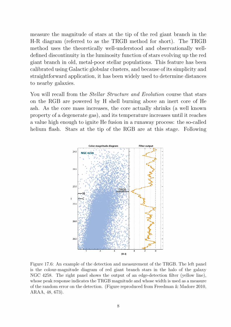
measure the magnitude of stars at the tip of the red giant branch in theH-R diagram (referred to as the TRGB method for short). The TRGBmethod uses the theoretically well-understood and observationally well-defined discontinuity in the luminosity function of stars evolving up the redgiant branch in old, metal-poor stellar populations. This feature has beencalibrated using Galactic globular clusters, and because of its simplicity andstraightforward application, it has been widely used to determine distancesto nearby galaxies.

You will recall from the Stellar Structure and Evolution course that starson the RGB are powered by H shell burning above an inert core of Heash. As the core mass increases, the core actually shrinks (a well knownproperty of a degenerate gas), and its temperature increases until it reachesa value high enough to ignite He fusion in a runaway process: the so-calledhelium flash. Stars at the tip of the RGB are at this stage. Following

Figure 17.6: An example of the detection and measurement of the TRGB. The left panelis the colour-magnitude diagram of red giant branch stars in the halo of the galaxyNGC 4258. The right panel shows the output of an edge-detection filter (yellow line),whose peak response indicates the TRGB magnitude and whose width is used as a measureof the random error on the detection. (Figure reproduced from Freedman & Madore 2010,ARAA, 48, 673).

8

the He flash, the star quickly settles on the core He-burning horizontalbranch. The transition from the red giant to the horizontal branch occursrapidly, so that observationally the TRGB can be treated as a physicaldiscontinuity.

The tip of the red giant branch is best identified from colour-magnitudediagrams normally involving the near-infrared I-band, using a quantitativedigital filter technique, as illustrated in Figure 17.6.

The advantage of the TRGB method is its observational efficiency because,unlike Cepheid variables, there is no need to follow stars through a vari-able light cycle: a single-epoch observation through two filters is sufficient.Consequently, there are ∼ 5× more galaxies with distances determined bythe TRGB method than via the period-luminosity relation of Cepheids. Onthe other hand, red giant branch stars are not as bright as Cepheids, andtherefore cannot be seen as far. The two methods have been used togetherfor galaxies with distances d <∼ 20 Mpc, providing important consistencychecks.

17.5 The Maser Galaxy NGC 4258

The acronym Maser stands for Microwave Amplification by StimulatedEmission of Radiation, but a more accurate definition would substitute“Molecular” for “Microwave”. The first maser was built in a physics lab-oratory in the US in the mid 1950s, and it was the precursor to the laser.Masers have also been observed in astrophysical environments, in particu-lar in circumstellar regions, in the interstellar medium near regions of starformation, and in the accretion disks surrounding the massive black holesat the centres of galaxies with Active Galactic Nuclei, where the densityof molecules and of infrared photons that can pump their energy levels areboth high.

The archetypal AGN megamaser is in the nucleus of the Seyfert 2 galaxyNGC 4258 (a.k.a. M 106) in the Virgo cluster. The maser is detected viathe 22 GHz emission line of ortho-H2O which arises from trace amounts ofwater vapor (< 10−5 in number density) in small density enhancements inin a very thin, slightly warped accretion disk (see Figure 17.7).

9

Figure 17.7: Schematic representation of masers in the molecular gas disk in the centreof the Seyfert galaxy NGC 4258. The positions of the masing clumps are shown as theyappear on the sky, and superimposed on a model of a nearly edge-on warped disk. Basedon their measured Doppler shifts, the velocities of the clumps on the right (approaching)and on the left (receding) of this sketch follow a Keplerian r−1/2 curve, indicating a massof 3.8×107 M for the central black hole. The proper motions of the clumps near the lineof sight to the centre can be tracked over time as they move from right to left on theircircular orbits. Comparison of their angular velocities to their physical velocities givesa direct measurement of the distance to the galaxy. (Figure reproduced from D. Maoz,Astrophysics in a Nutshell, Princeton University Press).

The masing clumps act as dynamical test particles. A rotation curve ismeasured along the major axis of the accretion disk by monitoring thechange of maser radial velocities over time from single-dish radio obser-vations. Proper motions are measured on the near side of the disk minoraxis from observed changes in angular position in VLBI (very long base-line interferometry) images (a very high angular resolution, ∼ 300µarcsec)is required for this measurement). A comparison of the angular veloci-ties in the latter measurement with the absolute velocities in km s−1 inthe former then yields the distance to NGC 4258, d = 7.2 ± 0.2 Mpc (or(m −M) = 29.29 ± 0.06 mag). This value is in excellent agreement withthe distance to the galaxy deduced from the Cepheids and TRGB methods:(m−M) = 29.28± 0.04± 0.12 mag.

Attempts to measure distances to other megamasers have proved difficult sofar due to lack of sensitivity and the geometric constraint that the maserdisk be viewed nearly edge-on. However, the future looks promising forthis technique with the planned Square Kilometer Array, due to come intooperation in the next decade.

10

17.6 Tully-Fisher Relation

In 1977, Brent Tully and Richard Fisher found a strong correlation be-tween the total luminosity of a spiral galaxy (corrected to face-on inclina-tion to account for extinction) and the galaxy’s maximum (corrected toedge-on inclination) rotation velocity. In a general sense, the TF relationcan be understood in terms of the virial relation applied to rotationallysupported disk galaxies, under the assumption of a constant mass-to-lightratio. However, a detailed self-consistent physical picture that includes therole of dark matter in producing almost universal spiral galaxy rotationcurves still remains a challenge.

The TF relation is at present one of the most widely applied methodsfor distance measurements, providing distances to thousands of galaxiesboth in the general field and in groups and clusters. The scatter in thisrelation is wavelength-dependent, and appears to be greatly reduced atmid-IR wavelengths (see Figure 17.8). If the 3.6µm correlation stands thetest of time as additional calibrators enter the regression, a single galaxycould potentially yield a distance accurate to ±5%. All TF galaxies, whenobserved in the mid-IR, would then individually become precision probesof large-scale structure, large-scale flows, and the Hubble expansion.

Figure 17.8: Multiwavelength Tully-Fisher (TF) relations for all of the galaxies calibratedwith independently measured Cepheid moduli from the HST Key Project. Note thesignificantly reduced dispersion in the mid-IR dataset (panel d); however, a larger sampleof calibrators is needed to confirm the scatter and slope of the relation at the wavelengthof 3.6µm. (Figure reproduced from Freedman & Madore 2010, ARAA, 48, 673).

11

17.7 Type Ia Supernovae

One of the most accurate means of measuring cosmological distances outinto the Hubble flow utilizes the peak brightness of SNe Ia. The use ofType Ia SNe as standard candles was already discussed in Lecture 6 andwe will not repeat the relevant arguments here.

For Hubble constant determinations, the challenge in using SNe Ia remainsthat few galaxies in which SN Ia events have been observed are also closeenough for Cepheid distances to be measured. Hence, the calibration of theSN Ia distance scale is still subject to small-number statistical uncertain-ties. At present, the numbers of galaxies for which there are high-qualityCepheid and SN Ia measurements is limited to six objects (see Figure 17.9).Each of the six galaxies has between 13 and 26 Cepheids observed with HSTin the near-IR H-band.

Figure 17.9: A comparison of Cepheid and Type Ia supernovae distances. The authorsof this study (Riess et al. 2009) used the maser distance to NGC 4258 to calibrate theCepheids PL relation, and then adopted NGC 4258 as the calibrating galaxy for thesupernova distance scale.

12

17.8 Other Methods

Among other methods that have been used to determine H0 we brieflymention the following.

• Surface Brightness Fluctuations. In distant galaxies, the unre-solved stellar light within a given small solid angle is produced by Nstars. The fluctuations in surface brightness between adjacent smallareas is Poissonian, i.e. σ ∝ 1/

√N . Since the number of stars included

per unit solid angle increases with distance to a galaxy, N ∝ d2gal, we

have σ ∝ 1/dgal. The proportionality constant can be calibrated innearby galaxies with well-determined distances.

• Gravitational Lens Time Delay. The pathlengths to two imagesof the same source produced by a foreground gravitational mass aredifferent. If the source is variable, such as a quasar or a supernova,the delay in the arrival time of light from one image compared to theother is proportional to H−1

0 , and less dependent on other cosmologicalparameters, such as Ωm,0 and ΩΛ,0.

Initially, the practical implementation of this method suffered from anumber of difficulties, the most important being incomplete knowledgeof the mass distribution of the lens. However, more recent carefulstudies of, for example, the quadruple lens system B1608+656, haveresulted in improved precision, giving H0 = 71± 3 km s−1 Mpc−1.

• The Sunyaev-Zel’dovich Effect in X-ray Galaxy Clusters. Wealready discussed the S-Z effect in Lecture 10, where it was shown thatthe S-Z decrement (produced by the redistribution of CMB photonsfrom the Raleigh-Jeans to the Wien side of the blackbody spectrumthrough inverse Compton scattering off hot electrons in the intraclus-ter medium) is distance independent (see Figure 10.13). Since themeasured X-ray flux from a cluster is distance dependent, the combi-nation of CMB and X-ray observations can be used to deduce H0.

Again, the accuracy of this method has improved enormously in recentyears, with high signal-to-noise, high angular resolution, S-Z imagesobtained with ground-based interferometric arrays and high-resolutionX-ray spectra.

13

• Luminosity of Giant H ii Regions. It has been shown that theluminosity of a star-forming galaxy in the Hβ emission line, L(Hβ),is well correlated with the velocity dispersion, σ, measured from thesame spectral feature. While this technique is not yet competitivewith the others mentioned in this section, it could (with better obser-vations) be used to probe cosmic expansion to the highest redshifts,since the Hβ emission line is one of the strongest spectral features ofstar-forming galaxies.

• Cosmic Microwave Background and Baryonic Acoustic Os-cillations. As we saw in Lectures 10 and 14 respectively, statisticalmeasures of the CMB temperature and polarization fluctuations, andof the large-scale distribution of galaxies encode a number of cos-mological parameters. H0 is involved in combination with Ωm,0 andΩbaryons,0, so that an accurate independent determination of H0 canhelp break degeneracies.

17.9 Concluding Remarks

The long-standing debate as to the value of the Hubble constant has largely,but not completely, been resolved in the 21st century. In their comprehen-sive 2010 review, Freedman & Madore concluded that:

H0 = 73± 2 (random)± 4 (systematic) km s−1 Mpc−1

(see Figure 17.10). For comparison, the final (2015) analysis of the Planckobservations of the CMB gives H0 = 67.5±1 km s−1 Mpc−1. So, the issue isnot totally settled, although the two determinations agree to within ±1σ(if the systematic errors have been estimated correctly). Recently, thegeometric maser distance to NGC 4258 has been revised to 7.60 ± 0.17 ±0.15 Mpc which lowers H0 by ∼ 3 km s−1 Mpc−1, but also produces sometension with the zero-point of the Galactic Cepheids PL relation. Mostworks now adopt h ≡ H0/100 km s−1 Mpc−1 = 0.7 with an accuracy of5–10%.

Looking ahead, there are still strong motivations for improving furtherthe precision of the determination of the Hubble constant: not only doesH0 set the scale for all cosmological distances and times, but its accurate

14

determination is also needed to take full advantage of the increasinglyprecise measurements of other cosmological quantities. The on-going GAIAmission, and the imminent launch of the James Webb Space Telescopein particular, are expected to reduce the systematic uncertainty of thezero point of the Cepheid PL relation which underpins many subsequentastronomical distance measures. All of the other methods briefly reviewedin Section 17.8 have undergone major improvements in recent years andwill undoubtedly continue to improve in the years ahead.

Figure 17.10: Final results from the Hubble Space Telescope Key Project to measure theHubble constant. The lower panel shows the galaxy-by-galaxy values of H0 as a functionof distance. The vertical dashed line is drawn at 5 000 km s−1, beyond which the effects ofpeculiar motions are thought to be small. (Figure reproduced from Freedman & Madore2010, ARAA, 48, 673).

15