168 cover ii en - whycos portal (@ wmo)€¦ · 7.1.2 hydrological forecast operations a...

7.1 INTRODUCTION TO HYDROLOGICAL FORECASTING [HOMS J]

7.1.1 Scope

A hydrological forecast is the estimation of future states of hydrological phenomena. They are essen-tial for the effi cient operation of water infrastructure and the mitigation of natural disasters such as fl oods and droughts. In addition, they are becom-ing increasingly important in supporting integrated water resources management and reducing fl ood-induced losses.

Describing and predicting future water states can be categorized on the basis of how far into the future the event is forecast to occur. For instance, forecasts for various hydrological elements such as discharges, stages and velocities can be made from the start of the forecast up to different times in the future. The Technical Regulations provide the following classifi cation:(a) Short-term hydrological forecasts, which cover

a period of up to two days;(b) Medium-range hydrological forecasts, which

apply to a period ranging from 2 to 10 days;(c) Long-range hydrological forecasts, which refer

to a period exceeding 10 days.

This section discusses the importance and necessity of establishing an end-to-end hydrological forecast-ing programme, while 7.1.5 provides an introduction to the communications technology used to collect data and distribute critical forecasts and warnings to its users, and 7.2 describes the data requirements for hydrological forecasting. An overview is provided in 7.3 of the various forecasting techniques available, from simple index models to robust hydrological forecasting systems. Forecasting of fl ash fl oods (see 7.4) and snowmelt (see 7.6) have been dealt with in greater detail because there is a need for guidance material on those issues. Finally, water supply fore-casts are covered briefl y in 7.5. The discussion of hydrological forecasts in this chapter will be limited to predicting quantities of water.

7.1.2 Hydrological forecast operations

A hydrological forecasting service is composed of trained hydrological forecasters working with a

combination of real-time and historical data inputs, which can include use of radar and satellite as well as in situ data, communications hardware and software, hydrological models or modelling systems, meteorological models or model product or inputs and computer hardware. There are many ways to configure a hydrological forecasting service. There are, however, a critical number of factors that are necessary to ensure reliable delivery of a service meeting the needs of a diverse user community.

The operations concept of a hydrological forecast-ing service defi nes how the operational forecast service will operate on a day-to-day basis, as well as during fooding conditions. It covers the following points:(a) The mission and legal mandate of the

organization;(b) The users and the required products or

services;(c) Deadlines for dissemination;(d) How the hydrological forecasting service is

organized;(e) The hydrometeorological data network and

how it operates;(f) How the hydrologist will interact with the

meteorological forecasting offi ce;(g) Communications hardware and software used

to receive data and information as well as disseminate forecasts;

(h) How forecast products are produced;(i) What policies and standard operating proce-

dures will be followed to ensure best practices during routine and emergency conditions;

(j) The outreach of the hydrological forecasting service through the education and training of policymakers, emergency operations staff and the general public.

Sample products should be readily available for potential customers.

The mission and legal mandate of the hydrologi-cal forecasting service needs to be clearly defined. It is important that only one official source of forecast and warnings be authorized by law. Multiple sources of forecasts can result in conflicting information that produces confusion and reduces the possibility of effective response.

CHAPTER 7

HYDROLOGICAL FORECASTING

GUIDE TO HYDROLOGICAL PRACTICESII.7-2

The principal users of warning products are national, regional and local emergency management or civil defence organizations, the media, agriculture, industry, hydropower organizations, fl ood control managers, water transportation and municipal water supply organizations and the public. The requirements of hydrological data, forecast prod-ucts and warnings vary according to the targeted user community. It is essential for the hydrologist to understand user requirements so that data and forecast products can be tailored to meet their needs. There are many segments of a national econ-omy, such as transportation, emergency management, agriculture, energy and water supply, that have unique needs for such information. Recognizing these needs and providing data, fore-casts and products to meet them ensures that the hydrological forecasting service is of greatest bene-fi t to the community. Sophisticated users, such as hydropower organizations, require hydrometeoro-logical data, forecasts, inflow hydrographs and analyses to support the generation of electricity, while emergency management operations require simpler but more urgent forecasts and warnings.

The network, including stream gauges, precipita-tion gauges and the associated meteorological network, should be defi ned, taking into account the availability of data from all sources, such as the radar network and satellite downlink products. However, the continuous availability of such prod-ucts must be established before they are used on a regular basis in national hydrological forecasting services. Close cooperation between meteorological forecasting services and hydrological forecasting services is essential. The procedure, or system defi -nition, for the acquisition of data and forecasts, as well as analysis, are needed as input to hydrological forecasts and should be defi ned in the operations concept. Communications hardware and software used in fl ood forecasting systems depend on the infrastructure available in the country concerned. However, modern data communication systems, such as satellite and the Internet, provide a variety of choices and should be utilized appropriately.

It is important to assess staff requirements such as the number of technicians or professionals needed to run the centre during routine and emergency operations. Their roles and responsibilities, work-ing hours and the continuous training needs of forecasters should also be addressed.

Hydrological forecasting programmes must be reli-able and designed to operate during the most severe fl oods. The greatest benefi ts for an effective hydro-logical forecasting programme occur when fl ooding

is severe, widespread and/or sudden. Normally, there is a greater strain on resources during extreme events such as fl oods. The operation of the centre during extreme events must be well defi ned. In such instances, there is generally an increase in data fl ow and staffi ng needs, as more products must be delivered to more users with short deadlines. Frequently the hours of operation must be expanded to meet higher demands for service.

During routine conditions, the staff of a hydrologi-cal forecasting service collect data and quality-control information, receive and analyse meteorological forecasts, run hydrological models and forecasting systems, assess present and future hydrological conditions and produce forecast prod-ucts for distribution to users. During non-forecasting portions of the day, hydrologists update data such as rating curves, evaluate operational performance, re-calibrate models and seek further means of improving the accuracy and timeliness of future forecasts.

It is never possible to achieve continuous,100 per cent reliability of hardware, software and/or power for operations even with dependable maintenance programmes. Therefore, a hydrological forecasting service must establish backup procedures to safe-guard future operations of all components: data collection; forecasting system operations, including backup of hardware, software and data; forecast dissemination and other communications systems; power, uninterruptible power supply and backup generators; and provision of an alternate site for operations if the location of forecast centre itself is damaged.

The key to making a forecast centre operationally reliable is to establish a robust maintenance programme. Unfortunately this can be an expensive undertaking, especially if the network is spread out and diffi cult to access. All hardware and software must be routinely maintained, otherwise the system may not function when most needed. In some countries, the hydrological forecasting service includes a system administrator, who is responsible for maintaining the communications and forecasting system.

7.1.3 End-to-end hydrological forecasting systems

Today’s hydrological forecasting systems are affordable and powerful. The degree of success in using these systems generally depends on the amount of training received by the hydrologists employing them. These systems are capable of

CHAPTER 7. HYDROLOGICAL FORECASTING II.7-3

producing forecasts for fl oods that occur in a few hours to seasonal probabilistic outlooks many months in advance for larger river basins.

Establishing a viable hydrological forecasting and warning programme for communities at risk requires the combination of meteorological and hydrological data, forecast tools and trained fore-casters. Such a programme must provide suffi cient lead time for individual communities in the fl ood-plain to respond. In case of fl ood forecasts, lead time can be critical in reducing damage and loss of life. Forecasts must be sufficiently accurate to promote confi dence so that communities and users will take effective action when warned. If forecasts are inaccurate, credibility is reduced and an adequate response is not made.

Experience and lessons from the past have demon-strated that an end-to-end hydrological forecasting and response system (see Figure II.7.1) consists of the following steps, which must be linked to achieve reduction in fl ood losses:(a) Data collection and communication;(b) Hydrological forecasting and forecast product

generation;(c) Dissemination of forecasts to users;(d) Decision-making and support;(e) Action taken by users.

The interaction of the technological components of the integrated end-to-end hydrological forecasting system can be represented as a chain composed of many links. Each link must be fully functional to benefi t the user community or population at risk. As with links in a chain, should one link not be func-tioning properly, the entire system breaks down. In other words, if a perfect fl ood forecast is generated but does not reach the population at risk, or no capa-bilities to take preventive action exist, then the forecast system does not serve its desired purpose.

7.1.4 Uncertainity and probabilistic forecasts

In general, the primary objective of hydrological forecasting is to provide maximum lead time with suffi cient accuracy so that users may take appropriate action to mitigate losses or optimize water management decisions. All forecasts contain uncertainty and one of the most successful ways of dealing with this is the use of ensembles. The uncertainty associated with a hydrological forecast starts with the meteorology. Given that all mesoscale atmospheric models attempt to model an essentially chaotic atmosphere, meteorology has been seen as the primary source of uncertainty for some years. In addition, hydrological model parameters and the model mechanics also contribute to the associated uncertainty or error in forecasts. Adequacy of data is generally the main limiting factor. If only observed hydrological data are used to generate forecasts, lead times may be so short that the utility of forecasts to users is of little value. By coupling hydrological models with meteorological forecasts that are the result of meteorologists implementing global and regional numerical weather prediction models and accounting for local climatological conditions, streamfl ow forecasts can be extended from many days to weeks in the future. Although coupling of models can indeed extend the lead time for users, it also increases forecast uncertainty.

Climatological or seasonal forecasting has now become a useful tool for managing water and reduc-ing the risk of flooding. Extreme events are correlated with major changes in atmospheric and ocean circulation patterns; once such patterns can be identifi ed, the potential for a lesser or greater degree of storm activity can be forecast. This infor-mation can then be used to improve emergency response and increase the degree of readiness of forecasting agencies.

Figure II.7.1. Integrated fl ood forecasting, warning and response system in integrated water resources management: a critical chain of events and actions

GIS toolsMathematical models

Sense wateravailability

Get datawhereneeded

Futurewater

availability

Watermanagement

and floodcontrol

decisions

Appropriateindividuals

andgroups

Tasks fromresponse

plansOrganizationsCivil society

RelocationSand bagging

Other responses

Data Communication Forecast Decisionsupport Notification Coordination Actions


When the probability of an extreme fl ooding event is forecast to be greater than normal, certain measures can be taken in anticipation of the events, for example, stockpiling sandbags, emer-gency food and water supplies, and moving high-value stored crops or goods from flood-prone areas. This is also a good time to create awareness among the public as to the potential for fl ooding, highlighting the actions that the public and others should take, and to carry out emergency-response exercises to test the degree of readiness. In some cases, emergency measures such as the temporary raising of fl ood protection barriers may be warranted. Recent developments in computing power have allowed global and regional atmospheric models to increase their spatial resolution. Local area non-hydrostatic models, for instance, have been successfully reduced to a spatial scale of approximately one kilometre. In addition, smaller-scale processes, such as convection and orographic enhancement, have been modelled more effectively.

Probability forecasting should not be confused with forecast error. The latter is internal to the model and data, and represents the error caused by model inadequacy and data error. Perhaps the best way to distinguish between them is to view probability forecasting as an expression of the range of outcomes that are possible in light of the conditions that may arise before the fore-cast date, whereas forecast error is a totally undesirable feature of the shortcomings of the state of forecasting science and of the available data.

The primary mechanism used to incorporate uncertainty directly has been to perturb the initial conditions of the non-linear partial differential equations describing the atmosphere using mesos-cale convective system approaches. However, most methods currently in use are suboptimal and still rely on a judicious choice being exer-cised by the forecaster. The ensemble Kalman fi lter is widely used to propagate and describe forecast uncertainty. The European Centre for Medium-Range Weather Forecasting (http://www.ecmwf.int) and other international agencies have been investigating the use of mesoscale convec-tive system-based ensembles in recent years and a large-scale intercomparison hydrological ensem-ble prediction experiment, which was launched in 2005. While this approach is indeed promis-ing, it has yet to be proven, and a considerable amount of work will be required to develop proce-dures for the propagation of uncertainty through complex model systems.

7.1.5 Dissemination of forecasts and warnings

Forecasts lose value with time. The faster data and forecasts can be sent to users, the more time can be applied to response, thereby saving lives, reducing property damage and enhancing the operation of water resources structures. Dissemination of fore-casts and warnings to communities and villages at risk of fl ooding is frequently a weak link in the end-to-end chain. Signifi cant progress in commu-nications technology allows for the rapid transmission of data, forecasts and information over large distances and to remote locations.

The delivery of hydrological products from a fore-cast service can be categorized as normal daily forecasts and non-routine urgent forecasts. Many users require the routine transmission of data and forecasts on a daily basis, in the form of a hydrolog-ical bulletin. Information is generally given for key rivers, reservoirs and other water bodies of interest to the region. Daily bulletins vary in their composi-tion and frequently include information about current values and trends of stages, discharges, tendency of stages and discharges, water tempera-ture, reservoir data such as pool and discharge, precipitation, hydrological forecasts and ice condi-tions, if prevalent. Figure II.7.2 provides an example of such a bulletin.

Many routine hydrological products can be produced based on user needs. Water supply fore-casts and fl ow summaries can be issued on a weekly and monthly basis. These summaries frequently provide fi gures and data for key locations in river basins that may include medium- and long-range forecasts with lead times of weeks, months, or seasons. Distribution of routine hydrological prod-ucts should be as widespread as possible, since many types of users can benefi t from data and fore-casts. Opening up data and forecasts to many users enhances the value of forecasting services and builds a constituency for such services, which is necessary if they are to sustain operations in the future.

The Internet is the best means of disseminating information. Although communication is hindered by bandwidth limitations in many developing countries, its use and accessibility is improving. Hydrological forecasting systems can make use of this channel of communication in their dissemination strategies for hydrological products. Other means of distributing products are the public media, use of continuous radio broadcasts and fax.


Figure II.7.2. Example of a hydrological bulletin (Finnish Environment Institute)


The composition and distribution of forecast and warning products for medium-term extreme events require that input data be assembled rapidly and that forecasts be made and reach the population at risk in enough time to trigger response measures that will minimize the impacts. Hydrological fore-casting centres should explore all available communication channels to reach the specific population at risk. Communication media commonly used are direct transmission lines, satel-lite, radio and landline to emergency operation centres and radio and television stations.

Under emergency conditions such as flooding, warning products should clearly identify the type of hydrological threat, the location of the predicted event, namely the rivers and streams involved, the magnitude of the event expected, such as the peak fl ood level at critical locations, the forecast time of occurrence of the peak and, if possible, when the river is expected to fall below warning or danger level. Further details, such as what portion of the infrastructure will be affected by the event, should be provided, if possible. Such information provides emergency response units with locations where action needs to be taken to conduct evacuations and road closures. As more data and information become available, fl ood-warning products should be updated and disseminated to the media and emergency-response offi cials.

Advances in coupling hydrological models with expanding geographical information datasets have resulted in the development and implementation of high-visual hydrological forecasting products.

This new class of hydrological products shows fl ood inundation produced by models linked to high-resolution digital elevation model data. By linking that data with hydrological model forecast eleva-tions computed for river channels, the area of fl ood inundation for the fl ood plain can be overlaid on top of detailed digital maps of human infrastruc-ture showing how forecast fl ooding will impact a given location. An illustration of a fl ood map prod-uct is provided in Figure II.7.3.

7.1.6 Decision support

Organizations responsible for water resources management use decision-support tools to provide guidance for the operation of infrastructure. Forecasts for water management are needed to plan effective use of water, ranging from hydroelectric power generation to water supply and irrigation. Measures taken by managers can have signifi cant negative consequences if future water availability is not considered. If hydrological forecasts are availa-ble, water resources managers can operate water supply systems to better meet water demand and minimize the potential for confl ict.

Flood losses can be reduced if communities and countries invest in fl ood preparedness and response planning prior to the occurrence of the event. Emergency service organizations are responsible for establishing fl ood-response plans that outline the role of various national, provincial and local organ-izations in protecting life and property. This link in the end-to-end chain includes setting up evacua-tion routes, educating the population at risk of the

Figure II.7.3. Flood map inundation forecast for Hurricane Mitch fl ood in Tegucigalpa, Honduras


flood hazards and establishing procedures and training personnel to respond well in advance of the occurrence of a fl ood.

The perfect fl ood forecast has no value unless steps are taken to reduce losses. In the end-to-end proc-ess, data and forecasts must be produced as quickly as possible to give users time to take action. In the case of fl ooding, especially fl ash fl ooding, time is critical. Understanding users’ needs and how fore-casts are used is important. There are a wide variety of users, ranging from federal response agencies to local governments, that have different roles and needs in responding to and mitigating losses. Users must understand the forecast or warning message for appropriate response to occur.

7.1.7 Cooperation with the National Meteorological Service

Although a few countries have a combined meteor-ological and hydrological service, in most cases the meteorological and water management authorities are separate. Indeed, they are seldom within the same government department or ministry. The provision of good weather forecast information, particularly in relation to severe precipitation events, is a vital part of a fl ood forecasting and warning operation. It is therefore important that close cooperation be developed between the National Meteorological Service and the fl ood fore-casting service.

Generalized meteorological forecasts are of little use to hydrologists; therefore, an initial step in developing cooperation should be taken to decide where value can be added to the meteorological information and how it can be structured to meet hydrological requirements. This will be largely a matter of improving the information on rainfall forecasts in terms of quantity – quantitative precip-itation forecasts – timing and geographic distribution. Typical forecast products are as follows:(a) Routine forecasts made on a daily basis, giving

information on rainfall, temperature and weather for 24–48 hours, and an outlook period of some 3–5 days;

(b) Event forecasts, particularly forecasts and warnings of severe events, such as heavy rain-fall, snow and gales, which have hydrological impacts. These should provide good quantita-tive and areal information over a lead time of 12–36 hours;

(c) Outlook forecasts for periods of weeks or months, or particular seasons. These are useful for planning purposes, especially with regard

to drought or cessation of drought conditions. Some national meteorological services, such as those of South Africa, Australia and Papua New Guinea, provide forecasts of El Niño activity where this is known to have direct impacts on weather patterns.

The national meteorological service and the hydro-logical agency must agree on the structure and content of forecast and warning products. This is usually achieved by an evolutionary or iterative process over time.

It is also useful for other weather service products to be provided to the hydrological agency. The most common products are satellite imagery and rainfall radar information. The information is transferred by dedicated data feeds, which will have a higher degree of reliability than informa-tion transferred through public service networks or available from Websites. A direct arrangement for data transfer by the national meteorological service also should ensure that updates are auto-matically provided, for example, every 3–6 hours for satellite imagery and every 5–10 minutes for radar scans. By using satellite and radar informa-tion, hydrological agency staff can make their own assessment and judgement of the current and immediate future weather situation. It is impor-tant that staff be adequately trained to do this; the national meteorological service has an important role in providing the necessary training through introductory and updating courses.

The aforementioned arrangements and facilities should be covered by a formal service agreement defi ning levels of service to be achieved in timeli-ness of delivery and accuracy of forecasts. The service agreement should also include the costs of service provision. In this manner, both parties can defi ne the economic costs and benefi ts in providing the service, and the value that the service may have in impact management.

7.2 DATA REQUIREMENTS FOR HYDROLOGICAL FORECASTS

7.2.1 General

Data requirements for hydrological forecasting depend on many factors:(a) Purpose and type of forecast;(d) Basin characteristics;(b) Forecasting model;(c) Desired degree of accuracy of forecast;


(e) Economic constraints of the forecasting system.

Data requirements vary considerably according to the purpose of the forecast. Operating a reservoir requires reservoir infl ow forecasts relating to short intervals of time and the volume of water likely to enter the reservoir fl ow as a result of a particular storm fl ood. Water-level forecasts relating to large, slow-rising rivers can be estimated easily by meas-uring the water level of upstream stations. Therefore, the data input in such cases will be the water level at two or more stations on the main river or its trib-utaries. However, for small, fl ashy rivers, apart from the observations of water level and discharge at relatively small intervals, the use of rainfall data practically becomes unavoidable.

Various considerations, discussed in subsequent sections, go into deciding what type of forecasting model should be used. Input data requirements for calibration and operational forecasts vary signifi -cantly from model to model. For example, in case of a simple gauge-to-gauge co-relation model which may be suitable for large rivers, the only data requirement may be water level at two or more stations. However, the use of a suitable comprehen-sive catchment model requires a number of other data.

Although the accuracy of the forecasts is of primary concern, the constraints in respect of economy and the relative importance and purpose of forecasting may permit a lesser degree of accuracy. In such situ-ations a model may be selected where data requirement may be less rigorous. However, for forecasts at critical sites, such as those located near densely populated areas or otherwise highly sensi-tive areas, greater accuracy is essential.

Apart from the type of data to be used for forecast-ing purposes, the information regarding data frequency, the length of record of data and data quality are equally important, and should be duly accounted for in any fl ood forecasting system plan-ning. Care must be taken to ensure that there is no bias between the data used to develop the forecast procedure or to calibrate models and data used for operational forecasting.

On the whole, the availability and quality of data needed to produce a forecast is improving. The number of automated gages and radars is increasing, while the quality of new satellites and rainfall estimation algorithms is producing enhanced inputs to hydrological forecasting procedures and forecast systems. A key issue in achieving data

reliability in hydrological forecasts is the maintenance of the data platforms and the communications system.

7.2.2 Data required to establish a forecasting system

Realistic hydrological forecasts cannot be produced without data. Data required for hydrological fore-casting, as discussed in the previous sections, can be broadly categorized as:(a) Physiographic;(b) Hydrological;(c) Hydrometeorological.

Data relating to Geographical Information Systems (GISs) are required for both calibration and for visu-alization of model states and outputs. The data consist of many types of land cover information such as, soils, geology, vegetation and digital eleva-tion model elevations. Hydrological forecasting system performance will depend on the quality and quantity of the historical data and GIS data used to establish parameters.

Hydrological data relating to river water levels, such as discharges, ground water level, water quality and sediment load, and hydrometeorological data deal-ing with evaporation, temperature, humidity, rainfall and other forms of precipitation, such as snow and hail, are key to hydrological forecasting. Some or all of the above data may be needed either for model development or for operational use, depending on the model. Over the past ten years, databases and database-processing software have been coupled with hydrological models to produce hydrological forecasting systems which utilize hydrological and or meteorological data and proc-ess the data to be used by hydrological models. The latter then produce outputs used by the hydrologist to forecast river fl ow conditions, including fl oods and droughts.

An adequate hydrometeorological network is the main requirement for fl ood forecasting. In most cases, the operational performance of the data network is the weakest link within an integrated system. In particular, for the forecasting of fl oods and droughts, there needs to be at least adequate precipitation and streamfl ow/stream-gauge data. If snowmelt is a factor, measurements of snow-water equivalent, extent of snow cover and air tempera-ture are also important. Therefore, when establishing a hydrological forecasting system, it is important to ask the following questions:(a) Are the rainfall and stream-gauge networks

satisfactory for sampling the intensity and


spatial distribution of rainfall and the stream-fl ow response for the river basin?

(b) Are the stream gauges operating properly, and are they providing accurate data on the water level and streamfl ow?

(c) Are the data communicated reliably between the gauge sites and the forecast centre?

(d) How often are observations taken, and how long does it take for them to be transmitted to the forecast centre?

(e) Are data available to users who need the infor-mation for decision-making?

(f) Are the data archived for future use? (g) Are the data collected according to known

standards, and is the equipment properly maintained and calibrated and the data quality controlled?

Analysing the existing network is the fi rst step. An inventory of available monitoring locations, param-eters, sensors, recorders, telemetry equipment and other related data should be made and presented in graphical form. In low relief basins, monitoring sites from adjacent basins should also be listed, as data from those sites can be very useful. An evalua-tion should be performed to identify sub-basins that are hydrologically or meteorologically similar. The main objective is to take advantage of existing hydrometeorological networks operated by various government agencies and the private sector that are relevant for the basin. In some respects, it is prefer-able that the network serve many purposes, as this may lead to broader financial support of the network.

The suffi ciency of networks can be determined according to forecasting needs, and required modi-fi cations should be noted. These could include new stream gauges, raingauges and other sensors in the headwaters, or additional telemetry equip-ment. In some cases, network sites may not be well suited for obtaining fl ow measurements or other data under extreme conditions. Structural altera-tions may be required. Interagency agreements may be needed for the maintenance and operation of the network.

There are many sources of such data, ranging from in situ manual observations to automated data collection platforms and remote-sensing systems. Automated data systems consist of meteorological and hydrological sensors, a radio transmitter or computer – data logger – and a downlink or receiver site that receives and processes data for applica-tions. There are many types of automated hydrometeorological data systems that utilize line-of-sight, satellite or meteor-burst communications

technology. The rapid transmission of hydromete-orological information is extremely useful to water stakeholders and users because it can be accessed instantaneously by many users by downlinks and/or the Internet. Radar is a very popular and power-ful, yet expensive, tool that can be used to estimate precipitation over large areas. The use of geostation-ary and polar orbiting satellites to derive large volumes of meteorological and hydrological prod-ucts is advancing rapidly. Remotely sensed data can now be used to provide estimates of precipitation, snow pack extent, vegetation type, land use, evapotranspiration and soil moisture, and to delin-eate inundated areas.

For information on the instruments to be used in collecting, processing, storing and distributing hydrological and related data, see Volume I of this Guide.

7.2.3 Data required for operational purposes

The basic parameters that control hydrological processes and runoff are initial conditions and future factors. Initial conditions are conditions existing at the time the forecast is made and which can be computed or estimated on the basis of current and past hydrometeorological data. Future factors are those which influence the hydrological forecast after the current time. It can be claimed that the most severe resource management issues exist under extreme condi-tions: in time, during fl oods and droughts; and in space, in arid, semi-arid and tropical areas and in coastal areas.

A key variable to be established is the time step needed to adequately forecast a fl ood for a given location. If the time step is six hours, for example, the data must be collected every three hours or even more frequently. In many cases, supplement-ing a manual observer network with some automated gauges may provide an adequate opera-tional network. The use of more and more data may become necessary to improve the model effi -ciency, which will most likely increase the costs. This is a major factor governing the choice for observation, collection and analysis of data to be used for development of a suitable model and for operational fl ood forecasting. More data entail more expenditure and more time in collection and analysis and man power, for example. Cost-effec-tiveness of the model vis-à-vis relative accuracy and consequences resulting therefrom should be duly considered when determining the data requirements.


Remote-sensing plays an important role in collect-ing up-to-date information and data in both the spatial and temporal domains. The use of remote-sensing techniques is vital in areal estimation, in particular of precipitation and soil moisture. Such techniques enhance seasonal forecasting capabili-ties; contribute to the development of storm-surge forecasting, drought and low-fl ow forecasting; and help improve risk management.

The rapid spread of the Internet throughout the world has not only produced an excellent mecha-nism to distribute hydrological data and forecasts to a diverse user community, but has also produced a rich source of data, forecasts and information of use to National Meteorological and Hydrological Services. The Internet provides a source of valuable information for hydrological forecast services. This may include meteorological and hydrological models, hydrological forecasting documentation, geographical information system data, real-time global meteorological forecasting products, hydro-meteorological data and hydrological forecasting information. A vast amount of data, software and documents are available for use, and these sources are growing daily. Some sample URLs, or uniform resource locators, are provided at the end of the chapter for reference.

7.3 FORECASTING TECHNIQUES [HOMS J04, J10, J15, J80]

7.3.1 Requirements for fl ood forecasting models

Given the recognized variability of climate and its expected infl uence on the severity, frequency and impact of fl oods and droughts, the importance of forecasting has increased in recent years. This section descibes the basic mathematical and hydro-logical techniques forming the component parts of any forecasting system. A brief discussion of the criteria for selecting the methods and determining the parameters is also provided. Examples of the use of these components for particular applications are given in 7.4 to 7.6.

Flood forecasting operations are centred around time and the degree of accuracy of the forecast. In fact, a professional assigned with formulating a forecast has to race against time. Clearly, the models to be used by forecasting organizations must be reliable, simple and capable of providing suffi cient warning time and a desired degree of accuracy. Model selection depends on the

following factors: amount of data available; complexity of the hydrological processes to be modelled; reliability, accuracy and lead time required; type and frequency of fl oods that occur; and user requirements.

A comprehensive model involving very detailed functions which may provide increased warning time and greater degree of accuracy may have very elaborate input data requirements. All input data for a specifi c model may not be available on a real-time basis. Therefore, from a practical point of view, a fl ood forecasting model should satisfy the follow-ing criteria:(a) Provide reliable forecasts with suffi cient warn-

ing time;(b) Have a reasonable degree of accuracy;(c) Meet data requirements within available data

and fi nancial means, both for calibration and for operational use;

(d) Feature easy-to-understand functions; (e) Be simple enough to be operated by operational

staff with moderate training.

Indeed, the choice should never be restricted to a specifi c model. It is always desirable to select and calibrate as many models as possible with a detailed note on suitability of each of the models under different conditions. These models should be applied according to the conditions under which they are to be operated.

Comprehensive models, which are rather compli-cated, generally require computational facilities such as computers of a suitable size. At many places, however, such facilities are not available. Sometimes suitably trained staff are not available; what is more, these machines cannot be operated because of recurring problems such as electricity failures. Therefore, both computer-based comprehensive models and simple types of model can be devel-oped. A computer-based technique can be used in general, and in case of emergency, conventional techniques, which are generally of a simple type, may be adopted.

Apart from the selection of different models, it is desirable to have a calibration of the models under different conditions. For example, a model may be calibrated with a suitably large data network; however, at the same time, a model must be cali-brated for a smaller network and give due consideration to the possible failures in observation and real-time transmission of some of the data. This will be helpful in utilizing the model even in emer-gency situations in which the data are not available from all the stations. This will require different sets


of parameters to be adopted under different conditions.

7.3.2 Flood forecasting methods

On the basis of the analytical approach used to develop a forecasting model, fl ood forecasting methods can be classifi ed as follows:(a) Methods based on a statistical approach;(b) Methods based on a mechanism of fl ood forma-

tion and propagation.

Forecasting methods in the form of mathematical relationships produced with the help of historical data and statistical analysis have been widely used in the past. These include simple gauge-to-gauge relationships, gauge-to-gauge relationships with some additional parameters and rainfall–peak stage relationships. These relationships can be easily developed and are most commonly used as a start-ing point while establishing a fl ood forecasting system. The use of artifi cial neural networks to fore-cast fl ood fl ows is another modelling approach that has recently gained popularity.

Increasingly, forecast procedures are based on more complete physical descriptions of fundamental hydrological and hydraulic processes. In many instances when forecast fl ows and stages are needed along rivers, hydrologists use rainfall-runoff models coupled with river-routing models. If precipitation is in the form of snow, snowmelt models are applied. These models vary in accuracy and complexity, ranging from simple antecedent index models to multi-parameter conceptual or process models. With advances in computing and telemetry devel-opments, forecasting models are now more fl exible in providing information and allowing new data and experience to be incorporated in real time.

There are many varieties of these basic categories of models, and most differ according to how hydro-logical processes are parameterized. Models can range from simple ones featuring a statistical rainfall-runoff relationship combined with a rout-ing equation to others characterized by a much higher degree of complexity.

Hydrological models can be classifi ed as lumped, semi-distributed or distributed. Models are either event driven or continuous. If a model is capable of estimating only a particular event, for example the peak fl ood resulting from a storm, it is known as as event driven. A continuous model is capable of predicting the complete fl ood hydrograph at a spec-ifi ed time interval. Model selection requirements include the following factors:

(a) Forecast objectives and requirements;(b) Degree of accuracy required;(c) Data availability;(d) Availability of operational facilities;(e) Availability of trained personnel for develop-

ment of the model and its operational use;(f) Upgradeability of the model.

Signifi cant progress over the past two decades has been made in improving the science and perform-ance of such models. However, performance usually varies according to the type of river basin character-istics being modelled, the availability of data to calibrate models and the experience and under-standing of the model by the operational hydrologist. There are a large number of public domain and proprietary models available for use in fl ood forecasting. Chapter 6 of this Guide reviews a wide range of currently available hydrological models.

7.3.2.1 Statistical method

The correlation coeffi cient measures the linear asso-ciation between two variables and is a widely used mathematical tool at the root of many hydrological analyses. Regression is an extension of the correla-tion concept that provides formulae for deriving a variable of interest, for example, seasonal low fl ow, from one or more currently available observations, such as maximum winter groundwater level (see Draper and Smith, 1966).

The formula for calculating the correlation coeffi -cient r between n pairs of values of x and y is as follows:

r =( x i − x )( yi − y )

i=1

n∑

( x i − x )2

i=1

n∑ ( yi − y )

2

i=1

n∑

(7.1)

where x =1

nx i and y =

1

nyii=1

n∑i=1

n∑

A lack of correlation does not imply lack of associa-tion, because r measures only linear association and, for example, a strict curvilinear relationship would not necessarily be refl ected in a high value of r. Conversely, correlation between two variables does not mean that they are causatively connected. A simple scatter diagram between two variables of interest amounts to a graphical correlation and is the basis of the crest-stage forecast technique (see 7.3.4 for verifi cation of forecasts).

If either x or y has a time-series structure, especially a trend, steps should be taken to remove this


structure before correlating, and caution should be exercised in interpreting its signifi cance. Time-series techniques may be applied (see 7.5.3) when previ-ous values of a variable such as river discharge are used to forecast the value of the same variable at some future time.

Likewise, regression equations have many applica-tions in hydrology. Their general form is as follows:

Y = bo + b1X1 + b2X2 + b3X3 + ... (7.2)

where X refers to currently observed variables and Y is a future value of the variable to be forecast. Regression coeffi cients estimated from observed Y and X values are indicated by b. The X variables may include upstream stage or discharge, rainfall, catchment conditions, temperature or seasonal rainfall. The Y variable may refer to maximum or minimum stage. The multiple-correlation coeffi -cient measures the degree of explanation in the relationship. Another measure of fi t, the standard error of estimate, measures the standard deviation of departures from the regression line in the calibra-tion set. The theory is explained in all general statistical texts.

Linear combinations of the variables are sometimes unsatisfactory, and it is necessary to normalize either the X or Y. A powerful transformation method

can be used to transform Y to YT by the following equations:

YT = (YT – 1)/T T ≠ 0YT = ln(Y) if T = 0

(7.3)

which encompasses power, logarithmic and harmonic transformations on a continuous T scale. A suitable T value can be found by trial and error as that which reduces skewness or graphically by using diagrams such as Figure II.7.4.

Non-linearity can also be accommodated in a regression by using polynomials, for example, by using Xi, Xi

2 or Xi3. Alternatively, non-linear regres-

sion using function-minimization routines offers a simply applied route to fitting parameters of strongly non-linear equations. The selection of a useful subset from a large potential set of explana-tory variables calls for considerable judgement and, in particular, careful scrutiny of the residuals, the differences between observed and estimated values in the calibration dataset. The circumstances giving rise to large residuals are often indicative of adjust-ments that need to be made. Advantage should be taken of computer facilities and graphical displays of residuals to explore a number of alternative combinations. The exclusive use of wholly auto-matic search and selection procedures, such as stepwise, stagewise, backward and forward selec-tion and optimal subsets should be avoided.

Figure II.7.4. Flow-duration curve of daily discharge

100

80

6050

40

30

20

10

8

6

4

3

2

10.5 1 2 5 10 20 50 80 90 95 98 99 99.5 99.8 99.9

Per cent of time daily discharge exceeded

Dis

char

ge (

m3

s–1 )


Examples of the application of regression to fore-casting problems are given in 7.3.2.3 and 7.4.7.

7.3.2.2 Soil moisture index models

The antecedent precipitation index is described in 6.3.2.2. This method has been a primary tool for operational forecasting in many countries. As a measure of the effect of precipitation occurring prior to the time of the forecast, it provides an index to the moisture in the upper level of the soil. The most frequently encountered indices are the ante-cedent precipitation index and the antecedent moisture condition. The moisture index methods have two main features with respect to their appli-cation to hydrological forecasting. First, because the index is updated daily, it is suited to an event type of analysis rather than continuous modelling. Thus, to apply this method to most forecasting, it is necessary to divide a precipitation period into events or to divide an event into separate precipita-tion periods. For example, during extended periods of precipitation interrupted by brief periods of little or no rainfall, the decision as to whether one or several storms are involved may be diffi cult.

The second feature is that the computed surface-runoff volume, when applied to a unit hydrograph, produces a hydrograph of surface runoff only. In order to synthesize the total runoff hydrograph, the base flow must be determined by some other method. The technique is of operational use only if event runoff is of importance and a simple approach is all that can be justifi ed.

7.3.2.3 Simplifi ed stage-forecasting methods

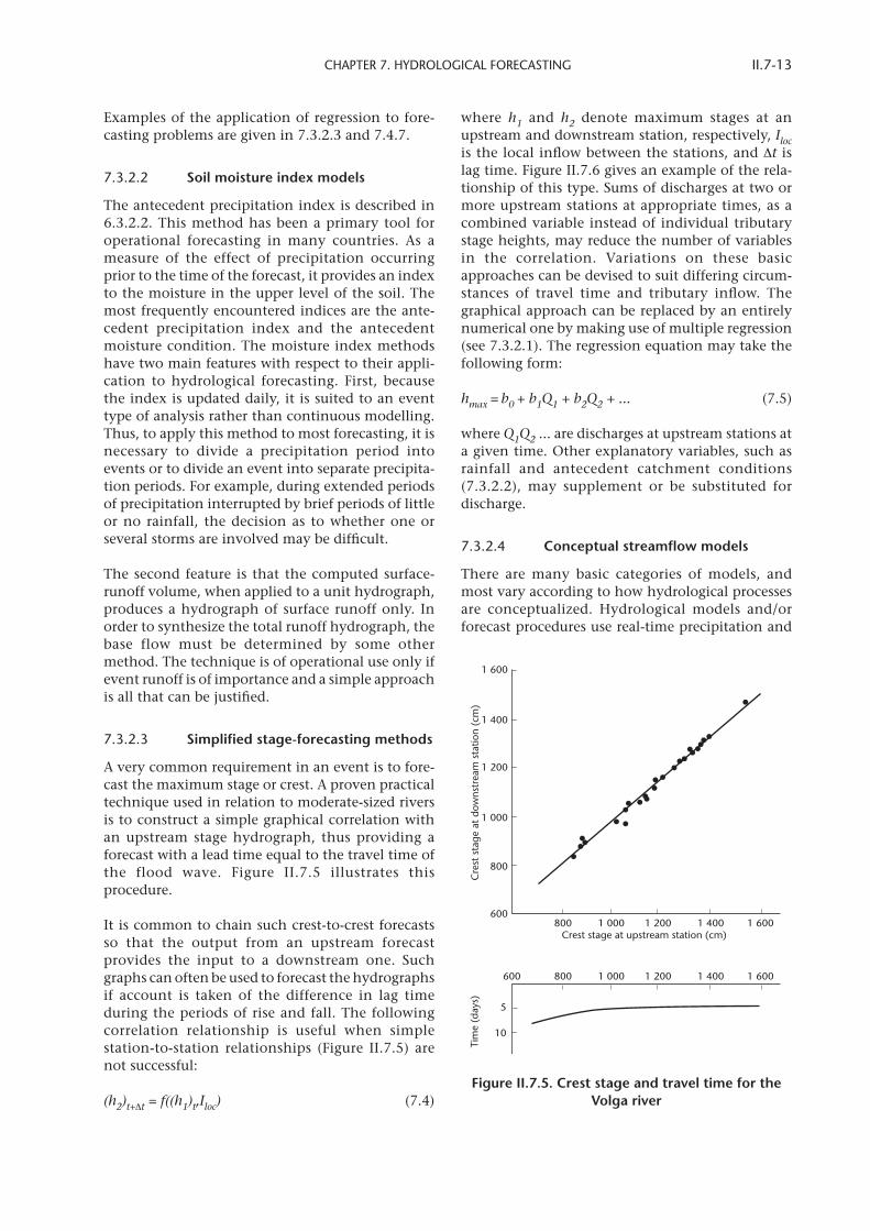
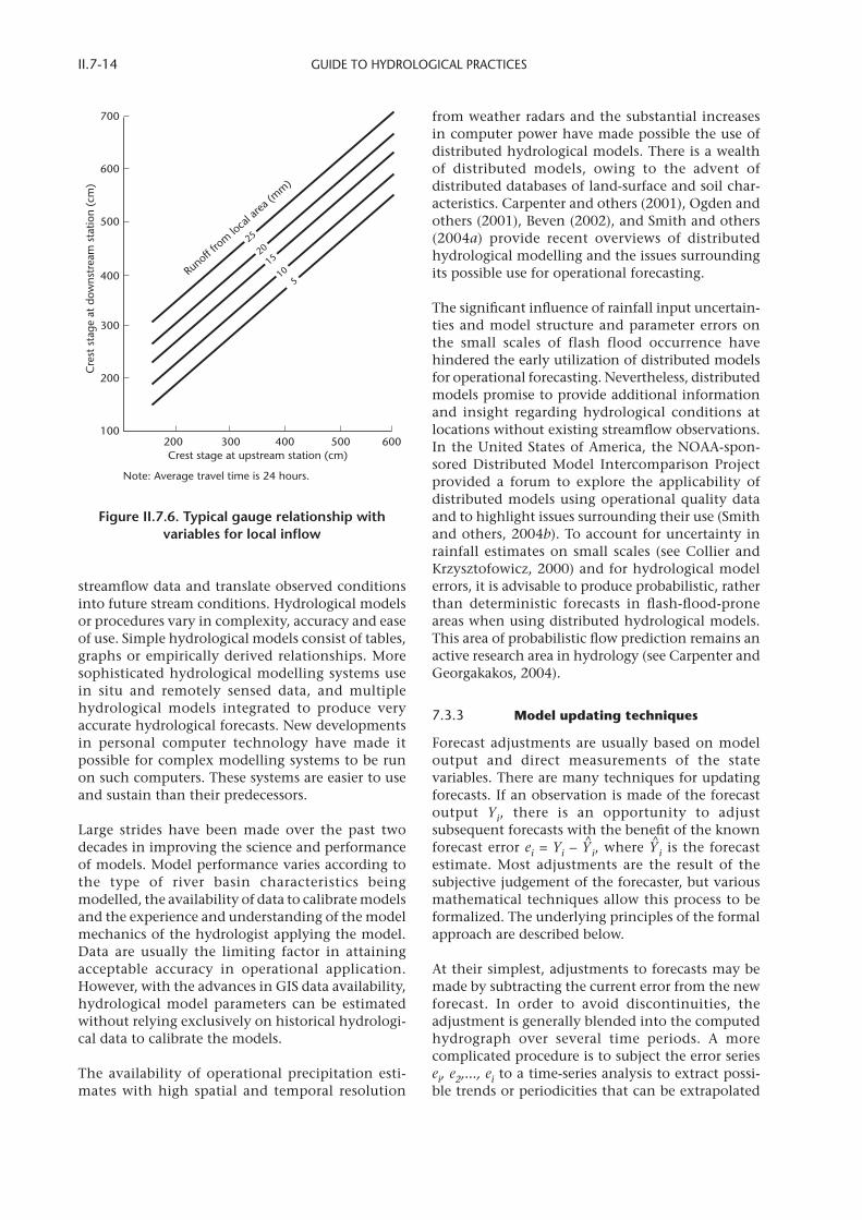
A very common requirement in an event is to fore-cast the maximum stage or crest. A proven practical technique used in relation to moderate-sized rivers is to construct a simple graphical correlation with an upstream stage hydrograph, thus providing a forecast with a lead time equal to the travel time of the flood wave. Figure II.7.5 illustrates this procedure.

It is common to chain such crest-to-crest forecasts so that the output from an upstream forecast provides the input to a downstream one. Such graphs can often be used to forecast the hydrographs if account is taken of the difference in lag time during the periods of rise and fall. The following correlation relationship is useful when simple station-to-station relationships (Figure II.7.5) are not successful:

(h2)t+Δt = f((h1)t,Iloc) (7.4)

where h1 and h2 denote maximum stages at an upstream and downstream station, respectively, Iloc is the local infl ow between the stations, and Δt is lag time. Figure II.7.6 gives an example of the rela-tionship of this type. Sums of discharges at two or more upstream stations at appropriate times, as a combined variable instead of individual tributary stage heights, may reduce the number of variables in the correlation. Variations on these basic approaches can be devised to suit differing circum-stances of travel time and tributary infl ow. The graphical approach can be replaced by an entirely numerical one by making use of multiple regression (see 7.3.2.1). The regression equation may take the following form:

hmax = b0 + b1Q1 + b2Q2 + ... (7.5)

where Q1Q2 ... are discharges at upstream stations at a given time. Other explanatory variables, such as rainfall and antecedent catchment conditions (7.3.2.2), may supplement or be substituted for discharge.

7.3.2.4 Conceptual streamfl ow models

There are many basic categories of models, and most vary according to how hydrological processes are conceptualized. Hydrological models and/or forecast procedures use real-time precipitation and

Figure II.7.5. Crest stage and travel time for the Volga river

1 600

1 400

1 200

1 000

800

600

5

10

800 1 000 1 200 1 400 1 600

600 800 1 000 1 200 1 400 1 600

Crest stage at upstream station (cm)

Cre

st s

tage

at

dow

nstr

eam

sta

tion

(cm

)Ti

me

(day

s)


streamfl ow data and translate observed conditions into future stream conditions. Hydrological models or procedures vary in complexity, accuracy and ease of use. Simple hydrological models consist of tables, graphs or empirically derived relationships. More sophisticated hydrological modelling systems use in situ and remotely sensed data, and multiple hydrological models integrated to produce very accurate hydrological forecasts. New developments in personal computer technology have made it possible for complex modelling systems to be run on such computers. These systems are easier to use and sustain than their predecessors.

Large strides have been made over the past two decades in improving the science and performance of models. Model performance varies according to the type of river basin characteristics being modelled, the availability of data to calibrate models and the experience and understanding of the model mechanics of the hydrologist applying the model. Data are usually the limiting factor in attaining acceptable accuracy in operational application. However, with the advances in GIS data availability, hydrological model parameters can be estimated without relying exclusively on historical hydrologi-cal data to calibrate the models.

The availability of operational precipitation esti-mates with high spatial and temporal resolution

from weather radars and the substantial increases in computer power have made possible the use of distributed hydrological models. There is a wealth of distributed models, owing to the advent of distributed databases of land-surface and soil char-acteristics. Carpenter and others (2001), Ogden and others (2001), Beven (2002), and Smith and others (2004a) provide recent overviews of distributed hydrological modelling and the issues surrounding its possible use for operational forecasting.

The signifi cant infl uence of rainfall input uncertain-ties and model structure and parameter errors on the small scales of flash flood occurrence have hindered the early utilization of distributed models for operational forecasting. Nevertheless, distributed models promise to provide additional information and insight regarding hydrological conditions at locations without existing streamfl ow observations. In the United States of America, the NOAA-spon-sored Distributed Model Intercom parison Project provided a forum to explore the applicability of distributed models using operational quality data and to highlight issues surrounding their use (Smith and others, 2004b). To account for uncertainty in rainfall estimates on small scales (see Collier and Krzysztofowicz, 2000) and for hydrological model errors, it is advisable to produce probabilistic, rather than deterministic forecasts in fl ash-fl ood-prone areas when using distributed hydrological models. This area of probabilistic fl ow prediction remains an active research area in hydrology (see Carpenter and Georgakakos, 2004).

7.3.3 Model updating techniques

Forecast adjustments are usually based on model output and direct measurements of the state variables. There are many techniques for updating forecasts. If an observation is made of the forecast output Yi, there is an opportunity to adjust subsequent forecasts with the benefi t of the known forecast error ei = Yi – Y^ i, where Y^ i is the forecast estimate. Most adjustments are the result of the subjective judgement of the forecaster, but various mathematical techniques allow this process to be formalized. The underlying principles of the formal approach are described below.

At their simplest, adjustments to forecasts may be made by subtracting the current error from the new forecast. In order to avoid discontinuities, the adjustment is generally blended into the computed hydrograph over several time periods. A more complicated procedure is to subject the error series ei, e2,..., ei to a time-series analysis to extract possi-ble trends or periodicities that can be extrapolated

Figure II.7.6. Typical gauge relationship with variables for local infl ow

700

600

500

400

300

200

100200 300 400 500 600Crest stage at upstream station (cm)

Note: Average travel time is 24 hours.

Runoff f

rom lo

cal a

rea (m

m)

25

2015

105

Cre

st s

tage

at

dow

nstr

eam

sta

tion

(cm

)


to estimate the potential new error e i+1, which can be used to modify the new forecast Y^ i+1.

There are two major types of real-time model updating:(a) Parameter updating, where the estimates of

some, and possibly all, of the model parameters are updated regularly on the basis of incoming data such as rainfall and fl ow. These data are obtained from conventional telemetry or the more modern supervisory control and data acquisition systems, also known by their acro-nym, SCADA;

(b) State updating, where estimates of the state vari-ables in the model, such as fl ow or water level, are updated regularly on the basis of incoming data.

Sometimes these updating operations are carried out in a fully integrated manner by using some form of parameter-state estimation algorithm such as the extended Kalman filter. Alternatively, they are carried out concurrently but in separate algorithms. These algorithms are normally known as recursive estimation algorithms because they process data in a recursive manner whereby new estimates are func-tions of previous estimates, plus a function of the estimated error. Examples of these algorithms are the recursive least squares algorithms, widely used in operational hydrology (see Cluckie and Han, 2000) and the recursive instrumental variables algo-rithm, as described in Young (1993).

The Kalman fi lter and the extended Kalman fi lter are recursive estimation techniques that have been applied to hydrological forecasting, but they require considerable mathematical and hydrological skills to ensure that the forecast model is in a suitable form for analysis.

The generic form of the recursive parameter estima-tion algorithm is as follows:

While the generic form of the state estimation algo-rithm is:

where y = g{xt} is the observed data that is related to the state variables of the model in some defi ned manner and Gt is a time variable matrix, often called the system gain, that is also computed recur-sively and is a function of the uncertainty in the parameter or state estimates. An algorithm that combines these two recursive estimation operations is often called a data assimilation algorithm (see Young, 1993).

However, a more conceptual technique for adjust-ing the output of a hydrological model may also be used. The method does not require any changes in the model structure or in the algorithms used in the model. Rather, this approach adjusts the input data and, consequently, the state variables in such a way as to reproduce more closely the current and previ-ous fl ows. These adjusted values are then used to forecast the hydrograph.

Forecast adjustments need not be based solely on the output of the model. It may also be accom-plished by using measurements of state variables for comparison with the values generated by the model. For example, one such technique uses observed measurements of the water equivalent of the snow cover as a means of improving the seasonal water supply forecasts derived from a conceptual model. Direct substitution of fi eld measurements for numerically generated values of the state varia-bles of the model would be incorrect because, in practice, model simplifi cations can result in such state variables loosing their direct physical identity.

7.3.4 Forecast verifi cation

Forecast verifi cation characterizes the correspond-ence between a set of forecasts and a corresponding set of observations. No forecast system is complete without verifi cation procedures in place to conduct administrative, scientifi c and user oriented verifi ca-tion of the forecasts.

A variety of statistics can be computed to evaluate forecast skill. The statistics to be used will depend on the type of forecast and the purpose of the fore-cast and of the verifi cation. A study of the utility of proposed metrics to effectively characterize the forecast skill should be conducted prior to imple-menting a verifi cation programme.

To be effective, a verifi cation system must include a forecast archive and the observations against which the forecasts are to be measured. In addition, a baseline forecast must be included to assist with the interpretation of the computed verification

Innovations process (one-step-ahead prediction)

a t = a t–1 + Gt{yt – y t|t–1}; y t|t–1 = f {a t–1, y

t–1} (7.6)

Model equation

Prediction: x t|t–1 = f {x t–1, a t–1}

Innovations process

Correction: x t = x t|t–1 + Gt{yt – y t|t–1} (7.7)


measures. Selection of the baseline forecast will depend on the forecast type to be verifi ed and the forecast process used to develop the forecasts. For short-term deterministic forecasts of less than two days, persistence is a useful baseline.

For longer-term forecasts and for probabilistic forecasts, climatological distributions or lagged climatology are more appropriate baselines. If the forecast process consists of several steps, additional intermediate data must also be archived to enable validation of each step in the forecast process. If possible, the input data used to compute the fore-casts should be archived to enable hindcast studies of possible forecast process updates. The data to be archived should include the observations, the input forecasts, such as precipitation and tempera-ture, and the model parameters, including rating curves. Joliffe and Stephenson (2003) are an excel-lent reference, providing more detailed information. In 1995, WMO developed MOFFS, the management overview of fl ood forecasting systems, to seek an internationally applicable basis for providing fast, focused information on the performance of fl ood forecasting systems based on exceedence of specifi ed trigger levels on rivers. The objective of MOFFS is to swiftly identify and high-light defi ciencies in the facilities and performance of individual fl ood forecasting systems in order that appropriate management action may be taken to remedy the defects before the next fl ood event occurs.

7.4 FORECASTING FLASH FLOODS [HOMS J04, J10, J15]

Flash fl oods are rapidly rising fl ood waters that are the result of excessive rainfall or dam break events. Rain-induced fl ash fl oods are excessive water fl ow events that develop within a few hours – typically less than six hours – of the causative rainfall event, usually in mountainous areas or in areas with exten-sive impervious surfaces such as urban areas. Although most of the fl ash fl oods observed are rain induced, breaks of natural or human-made dams can also cause the release of excessive volumes of stored water in a short period of time with cata-strophic consequences downstream. Examples are the break of ice jams or temporary debris dams.

7.4.1 National fl ash fl ood programmes

Prior to the advent and availability of high-resolution spatially extensive digital data from weather radars and from satellite platforms, and of

high-resolution digital terrain elevation data, forecasting of flash floods, as well as with the required spatio-temporal resolution, was not possible on a national scale. In recent years, however, high-resolution data have become available in most countries, and expanded computer capabilities have made it possible to develop national fl ash fl ood forecasting programmes.

7.4.1.1 Cooperation between hydrologists and meteorologists

Owing to the short concentration times of fl ash fl oods, the timely and accurate detection and short-term prediction of rainfall and streamfl ow and/or water levels are important ingredients of a success-ful fl ash fl ood forecast and warning system. This renders fl ash fl ood forecasting a truly hydrometeor-ological endeavour, which benefi ts much from close collaboration between meteorologists and hydrolo-gists in national and regional forecasting centres. In addition, the local nature of rain-induced fl ash fl oods requires detailed regional and local observa-tions, understanding and modelling of the heavy rainfall and the runoff-production/channel-routing processes in the fl ash-fl ood-prone areas, supported by databases of high resolution in both space and time.

7.4.1.2 Cooperation between national and regional or local agencies

Even when national flash flood forecasting programmes are in place, regional and local involve-ment is necessary for the operation of the systems to succeed. Individual regional and local physical settings signifi cantly affect fl ash fl ood genesis and development. The meteorological and hydrological situation may change from the time of data input at the national level to the time when regional and local response to forecasts is required. The error levels in the measurements by weather radar and satellite data vary considerably from place to place. Finally, individual end-users at the local level – the public at large, individual industries, water resources management agencies and so forth – are likely to have different requirements for fl ash fl ood warn-ings that may not all be addressed by the national fl ash fl ood forecast programme. This national and regional or local collaboration ideally involves regional forecast offi ces, local response agencies and end-users.

It may be necessary for end-users to develop addi-tional products that utilize the national fl ash fl ood forecasts and other ancillary information produced by the national forecast centres to address their


individual needs at the local level. For instance, this may include procedures for further refi nement of the forecasts for certain fl ood-stage levels not addressed by the national products, or installation and operation of local automated networks of raingauges and special-purpose radars in areas where national weather radars and satellites do not provide reliable data. In such cases, the national fl ash fl ood programme provides fl ash fl ood guidance.

7.4.1.3 Cooperation with end-users

For fl ash fl ood forecasts that are highly resolved in space and time, it is desirable to establish a significant forecaster-user collaboration programme that will serve several purposes: inform the users – the regional weather service offi ces, the local response agencies, the public at large or other end-users – as to what the national fl ash fl ood forecasts mean; provide information about forecast validation and the limitation of the national systems implemented; support decision-making at the local level; develop guide-lines for appropriate user action when warnings are issued; identify ways to receive feedback from the end-users as to the performance of the opera-tional system; and other purposes. This collaborative programme will in the long term help improve the local effectiveness of national fl ash fl ood forecast products.

In several countries, fl ash fl ood forecasts are dissem-inated by means of watches and warnings. If meteorological conditions conducive to heavy rain-fall are observed or foreseen for an area, a watch is issued on radio and/or television. This alerts resi-dents in the area to the potential occurrence of rainfall that could produce fl ooding. When fl ood-producing rainfall is reported, the watch is followed by a warning advising the residents in the area to take necessary precautions against fl ooding.

7.4.2 Local fl ash fl ood systems

There is a wide variety of fl ash fl ood forecasting and warning approaches implemented for specific gauged sites. They range from self-help procedures based on local networks of automated stream gauges to more sophisticated procedures that include local short-term rainfall and flow forecasting. These procedures are designed to provide early warning for local communities, utility companies and other regional or local organizations so that they can act immediately on receiving the warning. A few repre-sentative site-specific approaches are discussed below.

7.4.2.1 Self-help forecast programmes

Self-help fl ash fl ood warning systems are operated by the local community to minimize delays in the collection of data and dissemination of forecasts. A local fl ood warning coordinator is trained to prepare fl ash fl ood warnings based on pre-planned proce-dures or models prepared by qualified forecast authorities. The procedures are employed when real-time data and/or forecast rainfall indicate a potential for fl ooding. Multiple regression equa-tions provide an operationally simple fl ash fl ood forecasting technique that is summarized in a simple fl ood advisory table. The procedure is suita-ble for a range of different flood-producing conditions of rainfall, soil moisture and temperature.

The growing availability of microprocessors has led to an increased tendency to automate much of the data collection and processing that are required to produce fl ash fl ood warnings. Automatic rainfall and stage sensors can be telemetered directly to the computer that will monitor the data-collection system, compute fl ood potential or a fl ood forecast, and even raise an alarm. The most critical compo-nent in the self-help system is maintenance of active community participation in the planning and operation of the system.

7.4.2.2 Alarm systems

A fl ash-fl ood alarm system is an automated version of the self-help type of warning programme. A stage sensor is installed upstream of a forecast area and is linked by land or radio telemetry to a reception point in the community such as a fi re or police station that is staffed around the clock. This recep-tion point contains an audible and visual internal alarm and relay contacts for operating an external alarm. The alarm is activated when the water level at the sensor reaches a pre-set critical height.

7.4.2.3 Integrated hydrometeorological systems

These systems are more sophisticated state-of-the-art systems and are generally implemented by utilities and other regional or local organizations that maintain in-house hydrometeorological exper-tise. In most cases these systems provide the most reliable fl ash fl ood forecasts for specifi c locations. Typical implementations involve integrated hydrometeorological models, either conceptual or process based (see Georgakakos, 2002). The compo-nents of these models consist of a regional interpolator of operational numerical weather


prediction information to the scale of analysis, 100 km2 or less, a soil-water accounting model and a channel-routing model. To account for uncertain-ties in real-time numerical weather predictions and sensor-data configurations, state estimators or assimilators provide feedback to model states from available real-time observations. Various forms of the extended Kalman fi lter and non-linear fi lters have been used in these systems.

An example of the implementation and use of inte-grated hydrometeorological systems is the Panama Canal watershed fl ash fl ood forecast system: more information may be found in Georgakakos and Sperfslage (2004). The 3 300-km2 Canal watershed has been subdivided into 11 sub-catchments based on topography, stream gauge availability, reservoir location and local hydrometeorology (see Figure II.7.7). Short-term forecasts covering one- to six-hour periods are necessary to mitigate damage to Canal equipment and operations. A meteorolo-gist and a hydrologist operate the system and interpret the rainfall and fl ow forecasts.

There is a 10-cm weather radar and more than 35 automated ALERT-type raingauges in the region. The computational grid of the US National Weather Service operational numerical weather prediction

model ETA covers the region with an 80-km resolu-tion and provides large-area forecasts of atmospheric state twice daily with six-hourly resolution and a maximum lead time of several days.

The rainfall forecast component uses information from the 80-km ETA model and upper-air radio-sonde and surface meteorological data. The precipitation model produces sub-catchment rain-fall forecasts that are compared to the merged radar gauge estimates to produce a forecast error. These rainfall forecasts are fed into the soil water account-ing model of each sub-catchment that generates runoff and feeds the channel-routing model. A separate state estimator is used to update the soil water model states from real-time discharge observations.

An important aspect of local hydrometeorological systems is forecast validation for signifi cant fl ash fl ood events. This activity provides useful informa-tion to forecasters to assist them with the interpretation of the system forecasts and the trans-lation of these forecasts into warnings and watches. Typical least squares performance measures may be used, such as residual mean, residual variance, mean square error and coeffi cient of effi ciency, together with other measures of performance

Figure II.7.7. The Panama Canal watershed showing terrain elevation (1 km digital terrain model) and sub-catchments (Georgakakos and Sperfslage (2004))

Longitude °W

Latit

ude

°N

80.1 80 79.9 79.8 79.7 79.6 79.5 79.4 79.3

9.5

9.4

9.3

9.2

9.1

9

8.9

8.8

8.7

900

800

700

600

500

400

300

200

100

0


produced in collaboration with the forecast users, including errors in forecast water volume over a given duration, peak hourly fl ow timing and magni-tude. Figure II.7.8 is an example of a fl ash fl ood warning.

7.4.3 Wide-area fl ash fl ood forecasts

The ability to measure precipitation routinely with high spatial and temporal resolution and the avail-ability of high-resolution spatial databases for the land surface and subsurface have led to the emer-gence of fl ash-fl ood-scale, operational, wide-area forecasts produced by national agencies. Two main approaches may be identifi ed for the production of wide-area fl ash fl ood forecasts with high resolution: (a) those that use the concept of fl ash fl ood guid-ance and (b) those that are based on spatially distributed hydrological models. In either case, rainfall observations and forecasts highly resolved in space and time are necessary.

To obtain rainfall estimates on the scales required for fl ash fl ood forecasting, dense raingauge networks are needed. For national fl ash fl ood forecasting over large areas with high resolution, rainfall estimation on such small scales includes data from automated raingauges complemented by data from regional weather radars and/or satellite sensors. Different sensors measure different attributes of rainfall and a merged product is often computed as a best esti-mate that combines all available data. It is often useful to produce measures of uncertainty in the rainfall estimates because measurement errors vary from sensor to sensor and region to region.

Many studies discuss operational quantitative rain-fall estimation achieved by merging raingauge and weather radar data, ranging from the early results of Collinge and Kirby (1987) in the United Kingdom of Great Britain and Northern Ireland to more recent results reported in the United States by Fulton and others (1998) and Seo and Breidenbach (2002). In such cases, the spatial variability of the rainfall fi eld on fl ash fl ood occurrence scales is obtained mainly from weather radar data, while use of the automated raingauges is made to correct fi eld-mean or range-dependent bias of the weather radar estimates using a variety of procedures, as described, for example, by Cluckie and Collier (1991), Braga and Massambani (1997) and Tachikawa and others (2003).

Satellite rainfall data are often calibrated with weather radar data existing in similar hydroclimatic regions and/or any sparse local or regional auto-mated raingauge networks. Combinations of

polar-orbiting and geostationary satellite products are also under development (see Bellerby and others, 2001).

7.4.4 Flash fl ood guidance

The concept of fl ash fl ood guidance has been used for wide area forecasts of fl ash fl ood occurrence since the mid 1970s in the United States (Mogil and others, 1978). Flash fl ood guidance is the volume of rainfall of a given duration, for example, one to six hours, over a given small catchment that suffi ces to cause minor fl ooding at the outlet of the draining stream. The volume estimate is updated frequently and is used to assess the potential for fl ooding when compared with volumes of observed or forecast rainfall of the same duration and over the same small catchment.

Determination of fl ash fl ood guidance in an opera-tional environment requires the development of the following tools:(a) Estimates of threshold runoff volume of vari-

ous durations, done offl ine;(b) A soil moisture accounting model to establish

the curves that relate threshold runoff to fl ash fl ood guidance for various estimated soil mois-ture defi cits (Sweeney, 1992).

Early fl ash fl ood guidance operations used statisti-cal relationships to develop the required threshold runoff estimates from a variety of regional and local data, such as topographic and climate data. Using existing digital spatial databases of land-surface properties such as terrain, streams and land use or land cover, together with GIS, Carpenter and others (1999) set the threshold runoff estimation problem on a physical basis and provide methods for devel-oping objective threshold runoff estimates on a national scale with high resolution. For a given small catchment, the basic threshold runoff rela-tionship is as follows:

Qfl ood = Qp(R,tr) (7.8)

where Qfl ood is the fl ow that is considered likely to cause minor fl ooding at the catchment outlet, and Qp is the peak of the surface runoff over the catch-ment caused by the effective rainfall volume R, the threshold runoff, of the given duration, tr. The Qfl ood may be estimated by the fl ow of a given return period, for example, two or four years, or by hydrau-lic formulae for uniform steady flow at stream bankfull and at the catchment outlet. Synthetic or geomorphologic unit hydrograph formulations may be used to estimate Qp from R and tr. The use of bankfull fl ow and geomorphologic unit hydrograph


Figure II.7.8. Flash fl ood warning sign


formulations requires no calibration and produces threshold runoff estimates that are conservative in terms of fl ood damage.

Channel cross-sectional properties at the catch-ment outlet are required in order to estimate bankfull flow and the geomorphologic unit hydrograph runoff peak. Such estimates are typi-cally obtained from regional regressions of channel cross-sectional properties, that is, bankfull width, or hydraulic depth that use GIS-estimated catch-ment properties – area, stream length and average stream slope – as predictors. These regional regres-sions are based on data obtained from surveys of natural streams in the region of interest and are used to provide estimates of channel cross-sectional parameters in all of the small catchments of the region.

The resolution of the digital terrain elevation data limits the size of the smallest catchments for which threshold runoff analysis may be made. For instance, a 90-m resolution terrain database may be used to produce catchment properties, such as area and stream location, length and slope, with relative errors between +/–10 per cent and +/–25 per cent for catchments greater than 5 km2. For such catch-ments, up to a maximum size of 50 km2, typical errors of threshold runoff estimates based on GIS analysis of digital terrain elevation data can reach +/–30 per cent of the value estimated at sites with a full complement of hydrometeorological data.

Threshold runoff is the volume of effective rainfall of a given duration generated over a small catch-ment that is suffi cient to cause minor fl ooding at the outlet of the draining stream. Once the thresh-old runoff estimates have been obtained for the regions of interest or for the entire country, they are used in conjunction with real-time estimates of soil water deficit to produce threshold runoff. The procedure is outlined below (see Georgakakos, 2004).

Typically, the national forecast services run a hydro-logical model operationally over basins of area in the order of 1 000 km2 to produce streamfl ow esti-mates and forecasts at each of several forecast preparation times. Upon completion of these oper-ational forecast runs, the current estimates of the soil water indices, valid at the forecast preparation time, are stored. To support fl ash fl ood computa-tion under these initial conditions, the hydrological model is run offl ine in “what if” scenario runs with increasing amounts of rainfall volumes of the same given duration. These “what if” runs use the same initial soil water estimates produced by the model

during a normal operational run. The surface runoff volume produced by these runs is plotted against the volume of required rainfall of a given duration. This plot may then be interpreted as the relation-ship of threshold runoff (effective rainfall or surface runoff volume) to fl ash fl ood guidance (actual rain-fall volume). It is used with the estimated value of threshold runoff for the catchment to obtain the required fl ash fl ood guidance volume, both of the same given duration.

Estimates of most recent catchment rainfall volume of duration equal to the fl ash fl ood guidance dura-tion may then be used to determine whether a fl ash fl ood is imminent in a certain catchment. Likely fl ash fl ooding occurrence is indicated when the observed rainfall volume is greater than the fl ash fl ood guidance estimate. Following this procedure, maps of entire regions highlighting catchments with a high potential for fl ash fl ooding may be produced on regional and national scales. Similar maps may be produced showing the future poten-tial of catchments for fl ash fl ooding using forecast, rather than observed, catchment rainfall volumes of a given duration. The US National Weather Service uses a national operational implementation of fl ash fl ood guidance for forecasts of wide area fl ash fl oods. A regional implementation of fl ash fl ood guidance is operated for the countries of Central America. National programmes for collect-ing the necessary fl ash fl ood occurrence data to validate the fl ash fl ood forecasts produced on the basis of fl ash fl ood guidance are a necessary comple-ment to the operational forecast programmes.

7.4.5 Dam-break fl ash fl ood forecasting

Catastrophic fl ash fl ooding results when a dam fails and the outfl ow passes through the breach in the dam and inundates the downstream valley. Methods used to predict the fl oods that result from such fail-ures are described in 6.3.5.4.

In recent years, the development of GIS and digital terrain elevation data of high resolution has led to the production of risk maps for specifi c areas down-stream of existing dams. These inundation maps indexed with fl ood wave travel time information are useful when distributed to local offi cials down-stream of a dam site for the development of contingency evacuation plans.

7.4.6 Storm surges in rivers

Storm surges in the open sea are produced by wind and atmospheric pressure and can generate gravity waves that propagate upstream into rivers. Suitable


techniques to forecast the development and propa-gation of the storm surge in the open sea, such as the US National Weather Service SPLASH model (Jelesnianski, 1974) and its propagation into bays – as presented by Overland (1975) – are required to defi ne the surge at the river mouth, where it is then routed upstream via a suitable dynamic-routing technique. As the upstream movement of the grav-ity wave is opposed by the downstream fl ow, routing of the storm surge upstream may best be accom-plished by dynamic-routing techniques (see 6.3.5). Hydrological routing techniques or kinematic-hydraulic routing techniques are not suited to prediction of wave motions that propagate upstream. Also, the inertial components of the gravity wave that are ignored in the diffusion-hydraulic routing techniques are too important to be neglected in the case of a storm surge. A number of papers on tidal rivers have been published by the United Nations Educational, Scientifi c and Cultural Organization (1991). More recent applications involve the use of GIS to produce risk maps for areas prone to fl ooding by combined storm surge and fl ood waves (see publications of the WMO Tropical Cyclone Programme).

7.4.7 Urban fl ooding

Continued urbanization of natural fl ood plains has contributed to a sharp increase in loss of life and damage to property. Rapid demographic and social changes, coupled with increasing land prices and environmental concerns relating to water pollution and potential climate change characterized by increased variability and extreme magnitude, make advances in urban water management worldwide all the more urgent (Pielke and Downton, 2000; Dabberdt and others, 2000).

There are two types of urban fl ooding. First, urban areas can be inundated by rivers overfl owing their banks – this is fl uvial fl ooding. Areas of inundation are forecast from the specifi c river-stage forecasts. Second, urban fl ooding can occur in local drainage as a special case of fl ash fl ooding.

A considerable volume of literature has been published on urban hydrology and water manage-ment, for example, reviews in Urbonas and Roesner, 1993; Kovar and Nachtnebel, 1996; and Dabberdt and others, 2000. Unique characteristics of urban hydrology are large areas of impervious or near-impervious areas and the co-existence of both natural and technological drainage systems: sewers, levees, pumps, detention basins and the like. As a result, surface runoff production from rainfall is highly variable and non-homogeneous, and the

flow of water and contaminants is accelerated toward higher peaks of outlet hydrographs. High spatial-temporal variability in rainfall translates into high spatial-temporal variability in runoff, as the urban catchments do not signifi cantly dampen such fl uctuations. The technological drainage and improvements to the natural drainage make for earlier and higher peak flows. With respect to hydrological impacts, the flood prediction and control problem becomes severe for events with 5 to 100 years’ return period, while the water quality problem can be acute with storms occurring with short return periods of even less than two years.

Owing to the characteristics of the urban response to rainfall and contaminant forcing, very high spatial and temporal resolutions are required in data, models and controls over large urban areas in order to ensure effective water resources manage-ment (Dabberdt and others, 2000). Thus, digital terrain elevation data, distributed hydrological models and weather radar data – combined with in situ automated raingauge data and GIS – can be used to develop urban runoff forecast and manage-ment systems. (Cluckie and Collier, 1991; Braga and Massambani, 1997; Georgakakos and Krajewski, 2000; Kovar and Nachtnebel, 1996; Riccardi and others 1997). In areas where significant urban growth is combined with mountainous terrain and convective weather regimes (Kuo, 1993), there is a great need to develop urban water resources management systems capable of very high resolu-tion over large urban areas.

7.4.8 Flooding from local drainage

In this case, intense rainfall over the urban area may cause fl ash fl ooding of streets and property in low-lying areas or built-up areas in old waterways, underpasses and depressions in highways. Such fl oods arise primarily from inadequate storm-drain-age facilities, and are invariably aggravated by debris clogging inlets to pipes and channels or outlets of retention basins. Flood warning schemes similar to those outlined for fl ash fl oods can be employed. These usually consist of local automated fl ash fl ood warning systems or generalized warnings that are based on national fl ash fl ood guidance operations. It is also possible to target the fl ash fl ood guidance esti-mates for the urban environment on the basis of very high resolution digital spatial databases of terrain, drainage network, both natural and techno-logical, and existing hydraulic works.

On causeways subject to fl ooding, traffi c can be alerted by using lights activated in the same manner as the fl ash fl ood alarm system. Urban fl ooding


usually affects sewer systems, even when waste water and storm sewerage are piped separately. Forecasts of urban runoff can be helpful in the treat-ment of sewage and the handling of polluted fl ood water in combined systems. The opposite problem is the high level of pollution accompanying urban runoff. Since this is ultimately discharged into natu-ral watercourses, it leads to increased pollution with problems for downstream water users. The forecast-ing of pollution loads depends on forecasting urban fl ood runoff.

7.5 LONG-TERM FORECASTING

7.5.1 Water supply forecasting

Water supply forecasts are essential for the opera-tion of domestic, industrial, irrigation and hydroelectric water supply systems. Forecasts commonly take the form of fl ow volumes over specifi c durations: annual, seasonal or monthly. The duration depends on the nature of the demand and the amount of storage in the system. Since water supply forecasts cover a wider time span than meteorological forecasts, errors will always be inher-ent because of climatic events during the forecasting period. Therefore, it is recommended that several forecast values with probabilities of exceedance be issued (see 7.3.4).

The choice of the forecasting technique is governed by the character of the drainage basin, available data and user requirements. Water supply forecasts may be made by using three basic techniques:(a) Snowmelt forecasts;(b) Conceptual models;(c) Time-series analysis.

Snowmelt methods are used in basins where snowmelt runoff dominates the flow regime. Forecasting of snowmelt is described in 7.6. Normally, some measures of the snow-water equiv-alent and the basin losses can be related empirically to total seasonal runoff by regression techniques. Satellite measurements of snow cover have been related to the discharge of the Indus river, for exam-ple, and reasonable results have been obtained in this basin, where conventional ground data are very scarce. These methods are primarily suited to forecasts of total runoff volume and do not describe the time distribution of the runoff.

Conceptual models can be used for water supply forecasting by running the model repeatedly and using a number of historical climate time series as

inputs. The output becomes a range of forecasted values to which probabilities of exceedance can be assigned. Models used for water supply forecasts should be calibrated so that deviations between observed and simulated runoff volumes are mini-mized. Since short-term variations are of minor importance, simple model structures may yield satisfactory results.

Time-series methods may be useful for water supply forecasts, where discharge is a valid measure of the state of the basin. The forecast relationships are generally very simple to apply. Regression models in which seasonal runoff is forecast from previous hydrological and climatic variables may be regarded as a special case of time-series methods.

Long-term forecasts, especially of seasonal runoff, are often expressed in probabilistic terms: a statisti-cal distribution of possible runoff volumes is contingent on rainfall subsequent to the date when the forecast is made. One source of uncertainty is the future weather between the date of preparing the forecast and the operative date of the forecast. For example, if a regression-based forecast gives the following equation:

Qsummer = b0 + b1Rautumn + b2Rwinter

+ b3Rspring + b4Rsummer (7.9)

a less informative, probabilistic forecast can be issued after only receiving the rainfall data for the previous autumn and winter. The probabilistic component must take into account the distribution of possible spring and summer rainfalls that might occur.

Unless the forecast model is very simple, it is almost certain that it will be necessary to simulate possible Qsummer values either by repeated sampling from the distribution of Rspring and Rsummer values or by repeti-tively applying the model to the historical traces of Rspring and Rsummer. If the sampling approach is adopted, it will be necessary to incorporate any correlation that might be present between the inde-pendent variables. If the historical approach is used, at least 30 years of record is desirable to obtain a representative range of combinations. The applica-tion of this technique is not limited to regression models. Any hydrological forecasting model can be perturbed retrospectively by real or synthetic data to construct a distribution of possible outcomes. A more realistic description of the distribution of actual values is obtained if a noise term is included in the model. This can be accomplished by adding to each forecast a random number whose standard


deviation is equal to the standard error of the model estimate. A more detailed discussion is provided in Long-range Water-supply Forecasting (WMO-No. 587, Operational Hydrology Report No. 20).

7.5.2 Flow recession forecasting

Long periods without rain are a feature in many parts of the world, particularly where continental and highly seasonal tropical and subtropical climates prevail. The occurrence of prolonged dry periods is signifi cant for agriculture, which can be adapted to suit conditions by using particular prac-tices, growing crops adapted to the conditions or providing irrigation. Drought takes place when the period without rain extends beyond the normal duration, placing stress on plants and further depleting water resources. It is therefore important form an operational point of view to forecast drought or to provide projections on how long drought conditions will last.

There is no single, simple defi nition of drought, as its nature will vary with the climate type, and the impact of the drought, for example, water supply, irrigation and stock rearing. Where drought is a regular occurrence, its severity, which is a factor of duration and temperature, becomes important. Drought extremes may result from an early start relative to the normal dry season or a delay in the return of wet conditions, or a combination of both. A simple means of recording drought duration can be defi ned as follows:(a) Drought begins after a period of 14 days with-

out rain;(b) Drought ends after a period of 20 days during

which rainfall is recorded on 11 or more days;(c) As well as duration, intensity of drought can be

recorded by cumulative temperature, that is, in degree days.

The Palmer Drought Severity Index (Palmer, 1965) is widely used in the United States as a means of defining drought conditions. The method uses current and recent measurements of temperature and rainfall, which are mathematically related through local mean values to provide an index of severity between –4, very dry, to +4, very wet. The method lends itself very well to mapping and GIS displays and is routinely published on the Web by the Drought Information Center of the National Oceanic and Atmospheric Association (www.drought.gov).

The characteristic behaviour of a river and, catch-ment to drought can be expressed as a fl ow-duration curve and a recession curve. A fl ow-duration curve

is clearly a probability relationship taken over the whole of the historic record, and it is therefore possible to equate a current fl ow to a probability level, and thus project the situation for more extreme fl ows. A fl ow-recession curve is constructed by plotting the relationship between fl ows at set interval separations, for example daily, 5 days or 10 days; the size of interval is infl uenced by the total length of the dry season and size of catch-ment. Thus plotting Q at t0 and t–5 throughout the period of declining fl ow, a curve of the form:

Q(t) = Q0e–C(t–t0) (7.10)

is produced. Successive years of recession curves can be combined by eye to give a full recession rela-tionship. This allows the current situation to be assessed in terms of the overall catchment recession and to provide an estimate of possible future dura-tion and severity of projected conditions, for example, one or two months ahead.

Meteorological forecasts can be of value in drought management. Most major forecast services now give a long-range forecast for durations of two to six months. These are broad in their approach, and are usually expressed in terms related to average or extreme conditions.

Analysis of the falling limbs of hydrographs, or river recessions, is an important component of fl ood and low-fl ow analysis; in forecasting, however, its use is largely confi ned to low-fl ow forecasting. Some low-fl ow forecasting is achieved by analysing master recession curves on the large river basins, thus making it possible to forecast weeks or even months ahead. This type of forecasting is of value to hydro-power and irrigation schemes where the long-term supply of water is vital to optimal management practice. In addition, there is a highly specialized area where the principle long-term forecasts are produced by meteorologists using sophisticated global climate models. The subsequent hydrologi-cal work then focuses principally on the development of forecasts of fl ow and aquifer levels for use with reservoir control rules and water allocation strategies.

The most direct method is probably to perform a graphical correlation between the current fl ow or stage and flow or stage n days ago where n = 1, 2, 4, . . . (see 7.3.2.1). The defi ned relation-ship can be used to extrapolate forward in time if there are no disturbing infl uences, such as precipi-tation events. Departures from the most characteristic line can often be associated with natural or man-made phenomena, and this


information can also be brought to bear on any particular forecast.

7.5.3 Time-series analysis

A set of observations that measures the variation in time of a particular phenomenon such as the rate of fl ow in a river or the water level in a well or lake is described as a time series. A time series can be speci-fi ed in continuous or discrete time, depending on whether observations of a system state variable such as fl ow are made continuously or quantized into a discrete set of measurements which approxi-mate the variation of the state variable over time (see Kottegoda, 1980).

Since runoff is an indicator of the state of the drain-age basin, univariate time-series analysis may be used to establish forecast relationships. One such approach is to use autoregressive moving average models, (Box and Jenkins, 1976) that are well suited for use in basins with limited precipitation data, because only antecedent discharge is needed to make a forecast of this type:

Qt+1 = a0Qt + a1Qt–1 + aiQt–2 + ... + b (7.11)

where Qt+1 is the forecast with unit lead time and Qt–i are the measured values earlier than i time increments. Coeffi cients ai and b are estimated in the time-series analysis. In addition to the forecast value Qt+1, a time-series model can yield the distri-bution of possible deviations from the forecast value so that an estimate of forecast error is readily available. If a time-series forecast of monthly fl ows is to be reliable, then autocorrelation in the monthly time series must be large. This is the case in large rivers and in streams draining large aquifers and lakes. As a rule, however, forecasts are feasible only one to four months ahead. It is possible to include meteorological variables in a time-series model but, if such data are available, it is often preferable to make forecasts by using regression or a conceptual model. Time-series models may also be fi tted to the error series as discussed in the next section.

7.6 SNOWMELT FORECASTS

7.6.1 General

Many countries use forecast methods based on conceptual models of snowmelt runoff (see 6.3.3). Such methods make it possible to forecast snowmelt from observational and forecast meteor-ological data. Short- and medium-term forecasts are

possible for rivers and lowlands, and medium- and long-term forecasts, for streams in mountainous areas. Seasonal volume forecasts may be prepared for lowland and mountain basins, where snowmelt runoff produces a signifi cant portion of the total streamfl ow.

Snowmelt runoff is a characteristic feature of the regime of lowland rivers in temperate and cold climates and of some of the world’s largest rivers, even in tropical zones. Snowmelt runoff of many rivers accounts for 50–70 per cent of the annual runoff, and in dry regions the corresponding fi gure may reach 80–90 per cent. Runoff estimates are used in reservoir management and planning for consumptive use, power generation, public works and land development. As a result, a number of snowmelt hydrological models have been devel-oped to predict snowmelt runoff with a focus on capturing or predicting peak fl ows and volumes for engineering design and reservoir management purposes.

7.6.2 Snowmelt runoff processes in lowland and mountain rivers

During snowmelt, many of the processes that govern runoff in lowland and mountain river basins are similar, for example, snowmelt, water retention of snow, snowmelt infl ow to a basin, snowmelt runoff losses, water yield of a basin and time lag of snowmelt runoff to the outlet. However, some of the processes differ in two cases. For example, the year-to-year variation in the snowmelt runoff losses from snow and free water are signifi cantly greater in the plain regions than in mountainous river basins. More importantly, higher relief regions will have very different snow-covered distributions, with elevation playing an important role in the amount, redistribution and sublimation of the snowcover.

The total snowmelt runoff from lowland basins depends on the water equivalent of the snow cover at the time the snow begins to melt – the volume of precipitation occurs after the snow has begun to melt – and on the amount of water lost by infi ltra-tion and evaporation over the river basin. The fi rst factor can be determined to some degree by meas-urement; however, these measurements are highly landscape dependent (see Volume I, Chapter 3, of this Guide). The second factor, the subsequent amount of precipitation and the water losses during the runoff period, must be handled by a forecast procedure, either probabilistically or by assuming climatological average values. The possibility of using numerical weather prediction for short-term


forecasts is becoming a viable option in forecasting meteorological forcing. The third factor, snowmelt runoff loss from the basin, is controlled by the infi l-tration capacity of the soil and surface-depression storage, including large non-capillary pores in the upper soil layer. Evaporation losses are relatively small and vary little from year to year. Snowpack accumulation and ablation, especially during the spring thaw, are signifi cant inputs into daily hydro-logical forecasting systems, which in turn, are extremely useful for fl ood prevention and hydroe-lectric generation. The measurement and characterization of the distribution of snow within a catchment are critical to the prediction of subse-quent melt.

Volume I, Chapter 3, of this Guide states that catch-ment-based assessments of snow are typically derived from snow surveys and snow courses and, as a rule, recommends that in high relief regions, snow courses be at elevations and exposures where there is little or no melting until peak accumulation is achieved. In mild to low relief regions, these surveys need to represent the average snow condi-tions within a given catchment, and should be carried out on a variety of landscapes in order to properly depict the natural variability of the landscape.

Infi ltration of water into the soil during the snow-melt period is a factor that varies greatly from year to year, depending on the soil conditions. The rate of infi ltration into frozen soil and the total amount of water absorbed depend on the soil moisture content prior to freezing, the temperature, the depth of freezing and the soil’s physical properties. The size of the area covered by depression storage can be expressed mathe-matically as distribution functions of the depth of water required to fi ll these depressions. Such functions are relatively stable characteristics for each river basin.

7.6.3 Short- and medium-term snowmelt runoff forecasts

Short- and medium-term snowmelt runoff fore-casts for large river basins may be developed as follows:(a) Lowland river basins are divided into small,

partial basins, which are assumed to be hydrometeorologically homogeneous, each with an area of up to 15 000 km2, and the river system is divided into sections beginning with the upper reaches;

(b) Mountainous basins are divided into altitude zones. The number of zones depends on the

difference in altitude between the head and the mouth of the river system, as well as the variability of hydrometeorological condi-tions with the zone. In the experience of some hydrologists, the optimum altitude range for such zones is 200 to 400 metres with the number of zones around 20;

(c) The models are calibrated with hydrometeoro-logical data from preceding years;

(d) The forecast fl ows for the partial basins, or alti-tude zones for mountain areas, are routed to a downstream forecast point (see 6.3.5).

7.6.4 Long-term snowmelt forecasts

To devise a method for long-term forecasting of snowmelt runoff, it is necessary to establish water-balance relationships. This is preceded by the following tasks:(a) Determination of the relevant characteristics of

the river basin, such as topography, land-cover distribution and the nature of the soils;

(b) Determination of any factors governing the way in which water is absorbed by the soil and retained on the surface of the drainage area;

(c) Defi nition of the basic factors governing the loss of water in the river basin and the extent to which such factors vary from year to year;

(d) Determination of the role of precipitation occurring after the snowmelt has begun, in relationship to runoff, and of the variability of such precipitation;

(e) Evaluation of the accuracy of data for runoff, snow-water equivalent and precipitation.

Snowmelt runoff forecasts may be improved and extended by including probabilistically representative data and/or quantitative meteor-ological forecasts for the subsequent snowmelt period.

7.6.4.1 Seasonal snowmelt forecasts for the plains regions

The relationship between total snowmelt runoff Qn and the snow-water equivalent for plains areas may be expressed theoretically as:

Qn = (wn − f ) f ( yd ) d yd −o

wn−f

∫ f ( yd )d ydo

wn−f

∫ yd (7.12)

where wn is the snow-water equivalent and f is the total infi ltration during the snowmelt period, both expressed in millimetres. The function ƒ(yd) is the area distribution function in relation to the depth


of water, (yd), that is necessary to fi ll depressions on the river basin surface.

In the absence of infi ltration or when its intensity is potentially greater than the rate of snowmelt, equa-tion 7.12 can be simplifi ed as follows:

Qn = wn f ( yd ) d yd −o

wn

∫ f ( yd )d ydo

wn

∫ yd (7.13)

In this case, the runoff becomes a function of the snow-water equivalent and the infi ltration capacity of the basin.

The amount of water contributing to the seasonal snowmelt runoff is calculated for each year as the sum:

W = w– n + P– (7.14)

where w– n is the mean snow-water equivalent for the basin at the end of winter and P

– is the mean precipi-

tation during the runoff period, both expressed in millimetres.

The mean snow-water equivalent for the basin may be calculated as either an arithmetic mean or a weighted mean. The arithmetic mean method is used when the number of snow-measuring stations in the basin is suffi ciently large and when the spatial distribution of these stations is good. The weighted mean method is used when observation points are unevenly distributed over the area and/or when the distribution of the snow cover is irregular. To calcu-late the weighted mean of the snow-water equivalent, a map showing snowcover average distribution in the area is drawn.

In regions where a thaw may take place in winter, an ice crust often forms on the ground. If measure-ments are available, the amount of water contained in such crusts should be added to the snow-water equivalent. Very often, direct determination of soil-moisture conditions throughout the river basin, particularly in winter, is not feasible because of the lack of adequate data. This is the main reason why indirect indices are so common.

In dry steppe regions, the difference between precipitation and evapotranspiration characterizes the potential rate of infi ltration. In the humid forest zone where every year the autumn soil-moisture content is equal to, or greater than, fi eld capacity, this difference represents changes in the storage of the basin as a whole. The runoff caused by late autumn precipitation can also be used as an index of the retention capacity of river basins in these regions.

7.6.4.2 Seasonal snowmelt forecasts for mountainous regions

In mountainous areas, there tend to be consider-able differences in climate, soil and vegitation because of the range of altitudes. These features determine the nature of the snowmelt runoff and fl ow regime of the streams. Therefore, the most important characteristic of a mountain basin is its area–elevation distribution. The main sources of runoff are seasonal snow, which accumulates in the mountains during the cold season, and precipitation that occurs during the warm season of the year.

Owing to the long period between the beginning and end of the snowmelt period, long-term fore-casts of the seasonal fl ow of mountain rivers are feasible. The most favourable conditions for such forecasts exist where seasonal snow is the main source of runoff and the amount of summer precip-itation is relatively small.

Steep slopes, rocks and an extensive, highly perme-able deposit of rough rubble in mountainous basins create conditions in which the water fi nds its way into channels, mainly through layers of rubble and clefts in the rocks. Under such conditions, water losses do not vary greatly from year to year, and there should be a good relationship between seasonal runoff and the amount of snow in the basin. This relationship can be established empiri-cally if measurements are available for a number of years. However, in practice, determining such rela-tionships is often diffi cult.

7.7 FORECASTS OF ICE FORMATION AND BREAK-UP [HOMS J45]

7.7.1 General

Many rivers and lakes in middle latitudes freeze over in winter. The most important ice regime phases for which forecasts are made are as follows:(a) The fi rst appearance of ice;(b) The formation of complete ice cover;(c) The break-up of the ice cover; (d) The fi nal disappearance of all ice.

The ice regime of rivers is closely related to weather conditions. Thus, the dates of the appearance of fl oating ice and those of the formation and break-ing of the ice cover vary over a wide range from year to year. Ice forecasts are of great practical value


for navigation, but many other users apart from those in inland navigation are interested in these forecasts as well.

Exact relationships for calculating thermal and ice regimes are available; however, their application to ice forecasting is severely limited by the stochastic nature of parameters governing the equations, which vary over the time span between the forecast and the event predicted. This subsection discusses the different ice-regime forecasts that exist and short-term forecasts of ice formation and ice break-up.

Modern approaches to the short-term forecasting of ice phenomena are based on thermal balance (Buzin and others, 1989). For forecasts of autumn ice phenomena, formulae for the thermal balance at the boundary between a unit of surface of water and the adjacent atmosphere are used. Factors include direct heat exchange, solar radiation, turbu-lent heat and moisture exchange with the atmosphere, effective radiation, infl ow of heat from the Earth’s surface and groundwater, dissipation of stream energy as heat and the infl ow of thermal energy from precipitation which falls on the water surface and from the discharge of industrial and household waste waters. While the role of each of these factors in the thermal balance is different, the most important one is the exchange of heat through the open water surface.

Forecasts of the time when the ice cover breaks up are based on calculations of the tensile strength of the melting snow-ice cover, using formulae for the thermal balance and the derivation of a ratio between the durability of an ice cover and the destructive force at which the ice sheet is fractured. The latter is a function of the stream discharge, its water level and the rate at which they have changed over time.

Methods of modelling the formation and break-up of ice are covered in 6.3.6.3 of the present Guide.

7.7.2 Long-term ice forecasts

The development of methods for long-term fore-casting of ice phenomena usually includes the following tasks:(a) Consideration of the dates of ice formation

and break-up on rivers across the area under consideration, for example, average dates, vari-ability of the annual dates and the delineation of regions with uniform ice phenomena, the main mathematical instrument being statistical analyses;

(b) Synoptic analysis of conditions leading to freeze-up or ice break-up, in which the north-ern hemisphere is divided into typical regions, the main mathematical instrument here being discriminant analyses;

(c) Analysis of the distribution of stores of heat in the surface layers of oceans, such as the North-ern Atlantic and the northern Pacifi c Ocean; identifying the principles areas of interest, stores of heat within the limits of which render the greatest infl uence on processes leading to the formation and destruction of an ice cover on the rivers, the main mathematical instru-ment again being discriminant analyses;

(d) Determination of quantitative variables for atmospheric processes and ocean fi elds, such as expanding meteorological and ocean fi elds by orthogonal functions;

(e) Use of correlation analyses to determine the relationship between the time of ice occurrence and the variables representing the appropriate meteorological and ocean fi elds.

7.7.3 Ice jams and methods of forecasting high water levels

Dangerous rises in water level and resulting fl oods may occur during the formation of an ice cover or ice jam, and as a river’s ice cover or ice dam breaks up. Jam fl oods are especially hazardous because they occur in a cold season and sometimes remain for a long time. This causes sheets of water freeze to form an ice fi eld that can cover populated areas and can be almost impossible to remove. Often a sharp fall in water level occurs below the ice jam, starving intakes of water and interrupting water supplies.

On many rivers, maximum ice dam water levels exceed the highest water levels of spring and summer fl oods. Ice dams can form quickly and cause very rapid increases in water level, without any signifi cant increase in fl ow.

Ice jams arise more often in those reaches of rivers where ice cover grows out from each bank towards the middle and in an upsteam direction. The more slowly this process develops, the more ice is brought by the current under the frozen ice cover, causing contraction of the fl ow channel and raising the water level at the approach of the ice fi eld. Such characteristics of freezing are typical of large rivers fl owing towards the poles and rivers fl owing out of large lakes and after-bays of hydroelectric power stations.

River discharge during freezing, conditions for heat exchange, including air temperature, and the


position of the ice edge in relation to the cross-section are the primary factors to be taken into account in forecasting water levels from ice dams.

For a number of rivers where dangerous jams are frequently observed, physical–statistical relation-ships have been developed to account for these factors. The following example relates to the Neva river at Saint Petersburg (Buzin and others, 1989):

Hjam = 1.29HX1 + 0.53L + 0.24HG – 404 (7.15)

where HX1 is the average level of the Ladozhskoye lake in centimetres in November; L is the distance of the ice edge in kilometres from the Gorniy Institute station; HG is the water level at that station in centimetres.

Interestingly, by knowing only HX1, it is possible to issue good warnings of high water levels from ice jams more than one month in advance and to update these for three- to fi ve-day short-term fore-casts using equation 7.15.

A generalized method is available for deriving short-term forecasts of the maximum water level resulting from ice jams at critical locations on a river, includ-ing those for which there are no long time series of hydrological observations. Initial data required are the gradient of the given reach of the river, water discharge on the day that ice appears (Q0), air temperature during the freezing ice over the last few days and the curve Q = f(H) at the free ice chan-nel. For a forecast, it is necessary to defi ne a value of the critical gradient l’ given by:

l’ = 0.0154 g/c2 (1 – e) (7.16)

where g is the acceleration due to gravity; c is the Chezy coeffi cient; e is the porosity of ice fi elds esti-mated according to air temperature, where e = 0.25 at θ = –10°C and e = 0.55 at θ = –2°C.

If equation 7.16 is applied, the difference between I’ and the gradient of the open surface can be used with a special table developed for each hydrological post using the data of hydrological observations to defi ne a conversion factor kp, the winter dimension-less factor, between winter water discharge and the corresponding open channel discharge. The value of the discharge Qkr is calculated using the follow-ing equation:

Qkr = Q0e–k0Tice (7.17)

where k0 depends on the weather conditions during freezing; Tice is the duration of the ice run in days.

For example the coeffi cient k0 for the Amur river can be calculated using the following equation:

k0 = 0.005 – 0.00333TXI (7.18)

TXI is the average air temperature in Chabarovsk in October.

The maximum water level for an ice jam is deter-mined by using the reduced discharge Q’ (a hypothetical summer water discharge which raises water levels and would create an ice jam in winter) and summer curve Q = f(H). In this case it is neces-sary to calculate the reductioned discharge Q’ which can be estimated roughly as:

Q =Qkr

kp

' (7.19)

Spring ice dams that build up on rivers break-up downstream under the infl uence of spring fl ood waves from the upper part of the basin. This phenomena is particularly important for south-north-fl owing rivers in Canada and the northern parts of Europe and the Russian Federation. The ice break-up on these rivers takes the shape of a chain reaction of the consecutive formation and destruc-tion of ice dams of varying magnitude.

The maximum ice dam water level on a given river reach depends on many factors, which can be divided into those related to the process of ice cover formation and those related to its destruction. The most powerful dams and catastrophic fl oods arise when high water levels occur during ice cover formation. This can arise when high flows in autumn meet a channel constricted by ice slush, especially if the freezing of the river is accompanied by some movement of the ice cover (Buzin and others, 1989). It can also occur when a rapid rise during a spring fl ood in the upper reaches coincides with a sharp cooling at the limit of the ice cover in the reach under consideration so that the ice becomes particularly durable and forms an ice dam in a downstream reach.

The factors of the fi rst group make it possible in some river reaches, for example, on the Amur, Angara and Sukhona rivers, to predict maximum ice-dam water levels over periods of one to four months, using the following equation:

Ht,dam = 180 + 2.18 Hx (7.20)

where Ht,dam is maximum ice dam water level in centimetres; Hx is the water level at the period of ice cover formation in centimetres.


The addition of ice cover formation characteristics as parameters linked to the peculiarities of the spring processes has made it possible in the Lena river basin to predict the probability of occurrence of dangerous ice dam water levels during the ice break-up period for each of the four basic sections of the river with forecast lead times of 20 to 40 days. Using the relationship between ice thickness over the main part of the river and ice thickness at the main city within this part, it is possible to predict whether an ice dam will threaten the city or will form at another location. The probability of a correct prediction of dangerous levels is 80 per cent.

However, for many rivers where ice dams pose a particular risk, the development of methods for long-term forecasting is problematic and, where such forecasts are made, they frequently require correc-tion. For this reason, a number of methods have

been devised to provide short-term forecasts where ice dams occur each year. These forecasts are based on the physical and statistical relationships which take into account the major factors listed above. In a number of cases, a weather forecast for three to fi ve days is taken into account to estimate the character-istics of ice durability and probability of cooling.

Some recommended methods relate to the forecast-ing of ice dam water levels for any part of the river, even in the absence of long observation series. In such cases, it is possible to use the discharge curve, Q = f(H), and local meteorological data to calculate the relevant ice durability characteristics. The maxi-mum water level at an ice dam is determined from Q = f(H) and an appropriate Q’ is calculated from equation 7.19. In this case, Q’ is a conditional summer discharge, which could cause such a rise of water level, which occurs in ice dam formation. In equation 7.19, kp is the winter factor for the period

Figure II.7.9. River reach with an ice dam


of ice dam formation. This coeffi cient kp is derived from the link with characteristics of an ice cover expressed by the following equation:

kp = 8.13ϕhice

B⎛⎝

⎞⎠0.38

( k ice − 1) + 1 (7.21)

where ϕ is the relationship between ice durability on the last day before ice cover break-up and ice durability on the day when snow disappears from the surface of the ice, which can be derived using techniques described in a number of publications (Buzin and others,1989); hice is the thickness of ice in metres before ice cover break-up; B is the width of the river in metres; kice is the winter factor at a maximum water level at the beginning of freezing in the autumn (for various river catchments, kice = 0.65 0.85). The winter factor can also be calculated as follows:

k ice = 1 −1

1 .1 − 1 log g F (7.22)

where F is the catchment area in km2 located above an ice dam.

Where there is a river reach without tributaries above an ice dam, and there is a hydrological gauge in this part of the river (Figure II.7.9), it is possible to use the method of equivalent on ice phases discharges for the forecast of discharge at the ice dam (Qkr1):

Qkr1 = kp2 Qkr2 F1/F2 (7.23)

where kp2 is the winter factor for the date of ice dam formation in the upper section, Qkr2 is the discharge in the upper section, appropriated for a maximum ice dam level in the upper section according to summer curve discharges Q = f (H), and F1 and F2 are the areas of the basin closed by the lower and upper sections of the reach, F1 = F2 + ΔF.

The following Websites provide valuable informa-tion for hydrological forecasting services:http://edc.usgs.gov/http://k12science.ati.stevens-tech.edu/curriculum/

drainproj/reference.htmlhttp://nsidc.org/snow/http://snr.unl.edu/niwr/http://ulysses.atmos.colostate.edu/~odie/snowtxt.

htmlhttp://water.usgs.gov/http://water.usgs.gov/listurl.htmlhttp://www.afws.net/http://www.cpc.ncep.noaa.gov/products/expert_

assessment/threats.shtmlhttp://www.cpc.ncep.noaa.gov/products/fews/

http://www.dartmouth.edu/artsci/geog/fl oods/http://www.epa.gov/ebtpages/water.htmlhttp://www.hpc.ncep.noaa.gov/nationalfl oodout-

look/http://www.ibwc.state.gov/wad/rtdata.htmhttp://www.iwr.usace.army.mil/http://www.msc.ec.gc.ca/crysys/http://www.ncdc.noaa.gov/ol/climate/climateex-

tremes.htmlhttp://www.nohrsc.nws.gov/http://www.nws.noaa.gov/oh/hads/http://www.nws.noaa.gov/ohd/hdsc/http://www.nwstc.noaa.gov/HYDRO/RFS/

NWSRFS.htmlhttp://www.pecad.fas.usda.gov/cropexplorer/

global_reservoir/http://www.sce.ait.ac.th/programs/courses/IWRM/

Online_references.htmhttp://www.worldclimate.com/http://www.wri.org/watersheds/

References and further reading

Anderson, E. A., 1973: National Weather Service River Forecast System: Snow Accumulation and Ablation Model, Programs and Test Data. NOAA NWSHYDRO Technical Memorandum 17.

Appolov, B. A., G.P. Kalinin and V.D. Komarov, 1974: Course on Hydrological Forecasting. Leningrad, Gidrometeoizdat, 418 pp.

Barrett, C.B., 1999: Successful Development and Engineering of Global Integrated Water Management Systems, American Society of Civil Engineers, International Activities Committee, Roundtable Discussion paper, Washington, DC, 1999.

———, 2003: WMO-NOAA Hydrologic Forecasting Course, 14 October–7 November 2003, Kansas City, Kansas.

Barrett, C.B. and others, 1985: Hydrology Subcommittee of the Interagency Advisory Committee on Water Data, Guidelines on Community Local Flood Warning and Response Systems, Springfield, 1985.

Bellerby, T., M. Todd, D. Kniveton and C. Kidd, 2001: Rainfall estimation from a combination of TRMM precipitation radar and GOES multispectral satel-lite imagery through the use of an artificial neural network. Journal of Applied Meteorology, 39(12):2115–2128.

Bergstroem, S., 1976: Development and Application of a Conceptual Runoff Model for Scandinavian Catchments. SMHI Rapporter No. RH07, Hydrological Oceanography.

Beven, K., 2002. Towards an alternative blueprint for a physically based digitally simulated hydrologic response modelling system. Hydrological Processes, 16:189–206.


Borovikova, L.N., Y.M. Denisov, E.B. Trofimova and I.D. Shencis, 1972: Matematicheskoe modelirovanie processa stoka gornyh rek (Mathematical modelling of the runoff formation for mountain rivers). Trudy Sredaznigmi, Vyp. 61(76).

Borsch S.V. and T.P. Silantjeva, 1987: Method of the short-term and medium-term forecast of open-ing of the rivers on the basis of the generalized dependence. The methodical instructions. Moscow, Hydrometeorological center of USSR, pp. 28.

———, 1989: The improvement of the method of account of an ice cover destruction at the rivers and reservoirs. Report of the Hydrometeorological Center of USSR. v. 309, pp. 113–120. (in Russian).

Box, G.E.P. and G.M. Jenkins, 1976: Time-series analysis: Forecasting and Control. San Francisco, Holden-Day.

Braga, B., Jr. and O. Massambani, (eds.) 1997: Weather Radar Technology for Water Resources Management. Montevideo, UNESCO Press, 516 pp.

Brier, G.W. and R.A. Allen, 1951: Verification of Weather Forecasts. Compendium of Meteorology, (T.F. Malone, ed.) American Meteorological Society, pp. 841–848.

Brun, E., P. David, M. Sudak and G. Brunot, 1992; A numerical Model to Simulate snow-cover stratigra-phy for operational avalanche forecasting, Journal of Glaciology, 38(128):13–22.

Buzin V.A., G.I. Bolotnikov and A.M. Filippov, 1989: Ice jams on the rivers – methods of study, account and forecast. In book: Problems of nowadays of hydrol-ogy. Leningrad, Hydrometeoizdat, pp. 220–231 (in Russian).

Carpenter, T.M. and K.P. Georgakakos, 2004: Impacts of parametric and radar rainfall uncertainty on the ensemble streamflow simulations of a distributed hydrologic model. Journal of Hydrology (in press).

Carpenter, T.M., K.P. Georgakakos and J.A. Sperfslage, 2001: On the parametric and NEXRAD-radar sensi-tivities of a distributed hydrologic model suitable for operational use. Journal of Hydrology, 254:169–193.

Carpenter, T.M., J.A. Sperfslage, K.P. Georgakakos, T. Sweeney and D.L. Fread, 1999: National thresh-old runoff estimation utilizing GIS in support of operational flash flood warning systems. Journal of Hydrology, 224:21–44.

Carroll, T. R.,1995: Remote-sensing of snow in the cold regions. 1995. First Moderate Resolution Imaging Spectroradiometre (MODIS) Snow and Ice Workshop; NASA/Goddard Space Flight Center, Greenbelt, Maryland. 3–14.

Chagnon, S.A., 1999: Record flood-producing rainstorms of 17–18 July 1996 in the Chicago metropolitan area. Part III, Impacts and responses to the flash flooding. Journal of Applied Meteorology, 38:273–280.

Cluckie, I.D. and C.G. Collier, eds, (1991): Hydrological Applications of Weather Radar, Environmental

Management, Science and Technology Series, Chichester, Ellis Horwood, 644 pp.

Cluckie, I.D. and D. Han, 2000: Fluvial Flood Forecasting, Journal of Water and Environmental Management. 14(8) Chartered Institution of Water and Environmental Management (CIWEM).

Colbeck, S.C. (ed), 1980: Dynamics of Snow and Ice Masses. New York, Academic Press, pp. 305–395.

Collier, C.G. and R. Krzysztofowicz, 2000: Special Issue on Quantitative Precipitation Forecasting. Journal of Hydrology, 239:1–337.

Collinge, V.K. and C. Kirby (eds), 1987: Weather Radar and Flood Forecasting. New York, Wiley, 296 pp.

Dabberdt, W.F., J. Hales, S. Zubrick, A. Crook, W. Krajewski, J. Christopher Doran, C. Mueller, C. King, R.N. Keener, R. Bornstein, D. Rodenhuis, P. Kocin, M.A. Rossetti, F. Sharrocks and E.M. Stanley Sr, 2000: Forecast issues in the urban zone, Report of the 10th Prospectus Development team of the U.S. Weather Research Program. Bulletin of the American Meteorological Society, 81(9):2047–2064.

Donald J.R., E.D. Soulis, N. Kouwen and A. Pietroniro, 1995: A land cover-based snow cover representation for distributed hydrologic models. Water Resources Research, 31:(4):995–1009.

Draper, N.R. and H. Smith, 1966: Applied Regression Analysis. New York, Wiley.

Evensen, G., 1994: Sequential data assimilation with a non-linear quasi-geostrophic model using Monte Carlo methods to forecast error statistics, Journal of Geophysical Research, 90(C5):10143–10162.

Finnerty, B.D., M.B. Smith, D.-J. Seo, V. Koren and M.G. Moglen, 1997. Space-time sensitivity of the Sacramento model to radar-gage precipitation inputs, Journal of Hydrology, 203:21–38.

Fleming, G., 1975: Computer Simulation Techniques in Hydrology. New York, Elsevier.

Fulton, R.A., J.P. Breidenbach, D.-J. Seo and D.A. Miller, 1998: The WSR-88D rainfall algorithm. Weather and Forecasting, 13(2):377–395.

Georgakakos, K.P., 2002: US corporate technology trans-fer in hydrometeorology. Journal of Hydroinformatics, 4(1):3–13.

Georgakakos, K.P., 2004: Analytical results for opera-tional flash flood guidance. Journal of Hydrology (in review).

Georgakakos, K.P. and J.A. Sperfslage, 2004: Operational rainfall and flow forecasting for the Panama Canal watershed. Chapter 16 in Rio Chagres, A Multidisciplinary Profile of a Tropical Watershed (R.S. Harmon (ed.)). Dordrecht, Kluwer Academic Publishers, 16.1–16.13 (in press).

Georgakakos, K.P. and W.F. Krajewski (eds.), 2000: Hydrologic Applications of Weather Radar. Special Issue of Journal of Geophysical Research – Atmospheres, 105(D2):2213–2313.


Ginzburg B.M., S.V. Borsch and N.D. Efremova, 2001: Methods of the background long-range and medium-range forecasting of dates of opening of the rivers of the European territory of Russia. Journal of Meteorology and Hydrology, 11:67–78.

Ginzburg B.M., S.V. Borsch, N.D. Efremova and M.I. Silnitskaya, 1998: A method for backgraund long-term prediction of ice appearance dates for rivers and reservoirs in European Russia and Byelorussia. Journal of Meteorology and Hydrology, 6:84–91.

Ginzburg B.M., S.V. Borsch, N.D. Efremova, M.I. Silnitskaya and K.N. Polyakova, 2002: Methods of long-range and medium-range forecasting of dates of the spring flood maximal level on rivers on European territory of Russia. Journal of Meteorology and Hydrology, 11:81–92.

Ginzburg B.M. and M.I. Silnitskaya, 2000: Influence of the oceans surface of temperature distribution on the on terms of opening of the rivers of the European territory of Russia. Journal of Meteorology and Hydrology, 6:86–91.

Gray, D.M. and D.H. Male (Eds.), 1981: Handbook of Snow: Principles, Processes, Management and Use. Toronto, Pergamon Press.

Hedstrom, N.R. and J.W. Pomeroy, 1998: Measurements and modelling of snow interception in the boreal forest. Hydrological Processes, 12(10–11):1611–1625.4.

Hydrometeoizdat, 1989: Guide on the hydrological fore-casts. The ice forecasts. Vol. 3. Leningrad, 168 (in Russian).

Jelesnianski, C.P., 1974: SPLASH II: General Track and Variant Storm Conditions. NOAA Technical Memorandum, NWS, TDL-S2. US Department of Commerce, March.

Joliffe, T. Ian and B.D. Stephenson, 2003: Forecast Verification A Practitioner’s Guide in the Atmospheric Sciences. Wiley, 240 pp.

Jones, H.G., J. Pomeroy, D.A. Walker and R.W. Hoham, 2001: Snow Ecology: an interdisciplinary examination of snow-covered ecosystems. Cambridge University Press, 377 pp.

Koren, V.I., B.D. Finnerty, J.C. Schaake, M.B. Smith, D.-J. Seo and Q.Y. Duan, 1999: Scale dependencies of hydrology models to spatial variability of precipita-tion. Journal of Hydrology, 217:285–302.

Kottegoda, N.T., 1980: Stochastic Water Resources Technology, London, Macmillan Press.

Kovar, K., and H.P. Nachtnebel (eds), 1996: Application of Geographic Information Systems in Hydrology and Water Resources Management. IAHS Publication No. 235. Wallingford, IAHS Press, Institute of Hydrology, 711 pp.

Krzysztofowicz, R., 1992: Bayesian correlation score: a utilitarian measure of forecast skill. Monthly Weather Review,120:208–219.

Kummerow, C., W. Barnes, T. Kozu, J. Shiue and J. Simpson, 1998: The Tropical Rainfall Measuring Mission (TRMM) sensor package. Journal of Atmospheric and Oceanic Technology, 15(3):809–817.

Kuo, C.Y. (ed.), 1993: Engineering Hydrology. American Society of Civil Engineers, New York, pp. 989–994.

Mogil, H.M., J.C. Monro and H.S. Groper, 1978: NWS flash flood warning and disaster preparedness programs. Bulletin of the American Meteorological Society, 59:690–699.

Munich Re, 2001: Topics, Annual Review: Natural Catastrophes 2000, Munich.

Murphy, A.H. and R.L. Winkler, 1987: A general frame-work for forecast verification. Monthly Weather Review, 115:1330–1338.

Murphy, A.H., 1988: Skill scores based on the mean square error and their relationships to the corre-lation coefficient. Monthly Weather Review, 116:2417–2424.

Murphy, A.H., 1996: General decompositions of MSE-based skill scores: measures of some basic aspects of forecast quality. Weather and Forecasting, 124:2353–2369.

National Oceanic and Atmospheric Administration and the United Nations Department of Economic and Social Affairs, 2004: Guidelines for Reducing Flood Losses, 87 pp.

National Research Council (NRC), 1991: Opportunities in the Hydrologic Sciences. Washington, DC, National Academy Press, 348 pp.

Ogden, F.L., J. Garbrecht, P.A. DeBarry and L.E. Johnson, 2001: GIS and distributed watershed models, II, Modules, interfaces and models. Journal of Hydrologic Engineering, 6(6):515–523.

Overland, J.E., 1975: Estimation of Hurricane Storm Surge in Apalachicola Bay, Florida. NOAA Technical Memorandum, NWS-17, US Department of Commerce, March.

Palmer, W.C., 1965: Meteorological Drought, Research Paper No. 45, US Weather Bureau. Washington, DC.

Pielke, R.A., Jr and M.W. Downton, 2000: Precipitation and damaging floods, Trends in the United States, 1932-1997. Journal of Climate, 13:3625–3637.

Pomeroy, J.W. and D.M. Gray (eds.), 1995: Snowcover Accumulation, Relocation and Management. National Hydrology Research Centre, Saskatoon, Sask. Canada. NHRI Science Report No. 7, 144 pp.

Pomeroy, J.W. and E. Brun, 2001: Physical Properties of Snow. In: Snow Ecology: An Interdisciplinary Examination of Snow-covered Ecosystems. (H.G. Jones, J.W. Pomeroy, D.A. Walker, R.W. Hoham, eds). Cambridge, Cambridge University Press, pp. 45–126.

Rango, A., J. Martinec, J. Foster and D. Marks, 1983: Resolution in operational remote-sensing of snow cover. Hydrological Applications of Remote-sensing and Remote Data Transmission, Proceedings of the


Hamburg Symposium, August 1983. IAHS Publ. No. 145.

Riccardi, G.A., E.D. Zimmermann and R.-A. Navarro, 1997: Zonification of areas with inundation risk by means of mathematical modelling in the Rosario region Argentina. In: Destructive Water, Water-Caused Natural Disasters, their Abatement and Control (G.H. Leavesley, H.F. Lins, F. Nobilis, R.S. Parker, V.R, Schneider, F.H.M. van de Ven, eds). IAHS Press, Institute of Hydrology, Wallingford, 123–135.

Seo, D.-J. and J.P. Breidenbach, 2002: Real-time correc-tion of spatially nonuniform bias in radar rainfall data using rain gauge measurements. Journal of Hydrometeorology, 3(2):93–111.

Shi, J.C., J. Dozier and H. Rott, 1994: Snow Mapping in Alpine Regions with Synthetic Aperture Radar. IEEE Transcations on Geoscience and Remote-sensing, 31(1):152–158.

Sittner, W.T. and K.M. Krouse, 1979: Improvement of Hydrologic Simulation by Utilizing Observed Discharge as an Indirect Input (Computed Hydrograph Adjustment Technique – CHAT). NOAA Technical Memorandum NWS HYDRO-38, February, US Department of Commerce.

Sittner, W.T., C.F. Schauss and J.C. Monro, 1969: Continuous hydrograph synthesis with an API-type hydrological model. Water Resources Research, 5(5).

Smith, M.B., K.P. Georgakakos and X. Liang, (eds), 2004a: The Distributed Model Intercomparison Project (DMIP). Special Issue of Journal of Hydrology (in press).

Smith, M.B., D.-J. Seo, V.I. Koren and co-authors, 2004b: The Distributed Model Intercomparison Project (DMIP): An Overview. Journal of Hydrology (in press).

Sweeney, T.L., 1992: Modernized areal flash flood guid-ance. NOAA Technical Report NWS HYDRO 44, Hydrology Laboratory, National Weather Service, NOAA, Silver Spring, MD, October, 21 pp. and an appendix.

Tachikawa, Y., B.E. Vieux, K.P., Georgakakos and E. Nakakita (eds), 2003: Weather Radar Information and Distributed Hydrological Modelling. IAHS Publications No. 282. Wallingford, IAHS Press, 323 pp.

Todini, E. and J.R. Wallis, 1978: A Real-time Rainfall Runoff Model for an On-line Flood Warning System. AGU Chapman conference on applications of kalman filtering theory and techniques to hydrol-ogy, hydraulics and water resources, Pittsburgh, Pennsylvania, 22–24 May 1978.

Twedt, T.M., J.C. Schaake and E.L. Peck, 1977: National Weather Service extended streamflow predic-tion. Proceedings of the western snow conference, Albuquerque, New Mexico, 19–21 April 1977.

US Bureau of Reclamation, 1960: Design of Small Dams. Appendix A, Washington, DC, pp. 413–431.

US Department of Commerce, 2002: Final Report on Hurricane Reconstruction Program, Central American and the Dominican Republic, May 2002.

United Nations Educational, Scientific and Cultural Organization (UNESCO), 1991: International Workshop on Storm Surges, River Flow and Combined Effects. 8–12 April 1991, Hamburg, A contribution to the UNESCO-IHP project H-2-2.

Urbonas, B.R. and L.A. Roesner, 1993: Hydrologic design for urban drainage and flood control. In: Handbook of Hydrology (D.R. Maidment, ed.), New York, McGraw-Hill Inc., 28.1–28.52.

Weaver, J.F., E. Gruntfest and G.M. Levy, 2000: Two floods in Fort Collins, Colorado, Learning from a natural disaster. Bulletin of the American Meteorological Society, 81(10):2359–2366.

World Bank, 2002: 2002 World Development Indicators. Washington, DC, World Bank, 405 pp.

World Meteorological Organization, 1969: Hydrological Forecasting, Technical Note No. 92, WMO-No. 228, Geneva.

———, 1975: Intercomparison of Conceptual Models Used in Operational Hydrological Forecasting. Operational Hydrology Report No. 7, WMO-No. 429, Geneva.

———, 1982: Long-range Water-supply Forecasting, edited by M. Dyhr-Nielsen. Operational Hydrology Report No. 20, WMO-No. 587, Geneva.

———, 1986: Intercomparison of Models of Snowmelt Runoff, WMO-No. 646, Geneva, Switzerland.

———, 1990: Hydrological Models for Water Resources System Design and Operation. Operational Hydrology Report No. 34, WMO-No. 740, Geneva.

———, 1992: Simulated Real-time Intercomparison of Hydrological Models. Operational Hydrology Report No. 38, WMO-No. 779, Geneva.

———, 1994: Guide to Hydrologic Practices, Fifth Edition, WMO-No. 168. Geneva, pp. 721–724.

——— and the United Nations Educational, Scientific and Cultural Organization, 1997: The World’s Water, Is there enough?.

Young, P.C., 1993: Concise Encyclopaedia of Environmental Systems, Pergamon Press, pp. 22.

168 cover ii en - whycos portal (@ wmo)€¦ · 7.1.2 hydrological forecast operations a...

Documents