1

1

16.513 Control Systems (Lecture note #7)

A big picture: one branch of the course

The linear algebra tools will also be useful for other objectives.

Vector spacesmatrices

Algebraic equations

EigenvaluesEigenvectors

Diagonal formCanonical form

Matrix functions,such as eAtDuCxy Bu;Axx

: toSolutions

• Last Time: – Generalized eigenvectors, Jordan form

– Polynomial functions of a square matrix, eAt

2

Review: diagonal form and Jordan form

All eigenvalues of A are distinct diagonalizable There are repeated eigenvalues,

e.gi with multiplicity k.• If (A-i I)= n - (A-i I)=k,

there exist k LI solutions to (A-i I)v=0 and theyare all eigenvectors. If this is the case for all repeated eigenvalues diagonalizable

• If (A-i I)=n - (A-i I) < k,there exist generalized eigenvectors, not diagonalizable, there exist Jordan blocks

2

3

Definition. A vector v is a generalized eigenvectorof grade k associated with if

,0vIA k

– What is the new representation w.r.t. {v1, v2, ., vk}? i.e.,

A[v1 v2 … vk] = [v1 v2 … vk]Ā

0vIAbut 1k

v, vDenote k ,vIAvIAv k1k

,vIAvIAv 1k2

2k

,vIAvIAv 21k

1

,0vIAvIA k1 11 vAv

212 vvAv

1k2k1k vvAv

k1kk vvAv

A Jordan block

..00

1::

0..0

0..1

A

4

Polynomial functions of a square matrix

Let f()=i=1kiAi be a polynomial function of A.

If A=QĀQ-1, then f(A) = Qf(Ā)Q-1. Let () be the characteristic polynomial of A.

Cayley-Hamilton Theorem: (A) = 0

Any polynomial can be expressed as a polynomial of degree n-1

3

5

Theorem. Given ACnn and a polynomial f) Let the

distinct eigenvalues of A be i, i=1,2,...,m, each with

multiplicity ni, (n1+n2+…+nm= n). Let

)f(λ)(λf ,dλ

λfdλfwhere ii

(0)

λλ

i

i

l

ll

1n1n10 λβλββ)g( λ

f(l)(i) = g(l) (i), l = 0, 1, ..,ni -1, i = 1, .., m

Then f(A)=g(A) iff

Under the above condition, the coefficients i’s can be determined

6

Definition: Given ACnn . Let the distinct eigenvalues of A

be i, i=1,2,...,m, each with multiplicity ni, (n1+n2+…+nm= n).

Let f() be a general function with {f(l)(i)} well defined.

Suppose that g() is a polynomial satisfying

f(l)(i) = g(l) (i), l = 0, 1, ..,ni -1, i = 1, .., m

Then f(A) g(A).

Generally, g is a polynomial of degree n-1.

General functions of a square matrix:

4

7

• Some properties of eAt;• Solution to a continuous-time system

DuCxyBu;Axx

Today:

Du[k]Cx[k]y[k]Bu[k];A[k]1]x[k

• Solution to the discrete-time system

• Equivalent state equations

8

Some properties for eAt

3!

tA

2

tAAtI

k!

tAe

3322

0k

kkAt

From the definition,

The following can be verified

;ee

;eee

I;e

1AtAt

AtAt)tA(t

0

2121

Caution: eA+B usually does not equal to eAeB. We only have eA+B=eAeB when AB=BA

5

9

More properties:

?

dted At

1k

1kkAt

!1k

tA

dt

ed

1k

1k1k

!1k

tAA AtAe AeAt

tt

edted

AeAe

dted AtAt

At

3!

tA

2

tAAtI

k!

tAe

3322

0k

kkAt

1-kkLet

0k

kk

!k

tAA

10

More properties:

?dτet

0

Aτ

0k

kkAt

!ktA

e

0k

1kkt

0

Aτ

!1k

tAdτe

0k

1k1k1

!1k

tAA

IeA At1 1At AIe

1k

kk1 II

k!

tAA

~ Assuming that A-1 exists

BI)A(eBdτeBdτe 1Att

0

Aτt

0

Aτ

This will be used to compute the output responseunder constant inputs.

k k1

k 1

A t=A

k!

kk 1

6

11

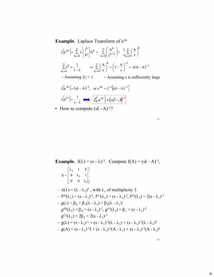
Example. Laplace Transform of eAt

k

0k

kAt A

!kt

e LL

0k1k

k

s

A

11

0k

k

~ Assuming || < 1

k

0k sA

s1

1k

0k sA

IsA 1AsIs

1 AsIeL At

~ Assuming s is sufficiently large

s

1e tL

,AsIe 1At L 11At AsIeor L

• How to compute (sI - A)-1?

12

Example. f() = (s - )-1. Compute f(A) = (sI - A)-1,

.

00

10

01

A

1

1

1

– () = ( - 1)3 , with 1 of multiplicity 3

– f(0)(1) = (s - 1)-1, f(1)(1) = (s - 1)-2, f(2)(1) = 2(s - 1)-3

– g() = 0 + 1( - 1) + 2( - 1)2

g(0)(1) = 0 = (s - 1)-1, g(1)(1) = 1 = (s - 1)-2

g(2)(1) = 22 = 2(s - 1)-3

– g() = (s - 1)-1 + (s - 1)-2( - 1) + (s - 1)-3( - 1)2

– g(A) = (s - 1)-1I + (s - 1)-2(A - 1) + (s - 1)-3(A - 1)2

7

13

1

211

31

211

1

λs

100

λs

1

λs

10

λs

1

λs

1

λs

1

g(A)A)(sI

000000100

I)λ(A,000100010

IλA 211

000000100

)λ(s000100010

)λ(s100010001

)λ(sg(A) 31

21

11

tλ

tλtλ

tλ2tλtλ

At

1

11

111

e00

tee0

/2ettee

L)L(e

14

• We will compute eAt;• Some of its properties; Solution to a continuous-time system

DuCxyBu;Axx

Today:

Du[k]Cx[k]y[k]Bu[k];A[k]1]x[k

• Solution to the discrete-time system

• Equivalent state equations

8

15

State-Space Solutions and Realizations

• Consider a linear system:

Solutions of Dynamic Equations

DuCxyBu;Axx

– A: nn real matrix; B: np real matrix

– C: qn real matrix; D: qp real matrix– Given x(t0) = x0 and u() A unique solution x(), y()– What is the solution?

x: n1u: p1 y: q1

16

• Recall that earlier we derived the solution for the input/output description based on superposition:

,τ)u(τ)dτG(ty(t)t

t0

τ)-(tgτ)-(tgτ)-(tg

τ)-(tgτ)-(tgτ)-(tgτ)-(tgτ)-(tgτ)-(tg

τ)G(t

qpq2q1

2p2221

1p1211

Questions:– Given system matrices, A,B,C,D, what is G(t)?

– What is the response due to initial state?

• Another approach is by using Laplace transform:

(s)uD]BA)[C(sIx(0)A)C(sI(s)y 11

─A downside: the Laplace transform of u(t) may be not available, you may need to approximate it.

9

17

State-Space Solutions

DuCxyBu;Axx The system:

Given x(0) and u(t) for t ≥ 0. The solution for x and y is

Du(t))d(BuCex(0)Cey(t)

;)d(Buex(0)ex(t)t

0

τ)A(tAt

t

0

τ)A(tAt

─ Clearly two parts: zero-input resp. + zero-state resp.─ Linearity also obvious. ─ We know how to compute eAt. The integration can

be done numerically through discretization.

1k

0i

i)ΔA(kk

0

τ)A(t )Bu(ie)d(Bue

G(t-)=CeA(t-)B

18

We first consider the state x: (*) Bu(t);Ax(t)(t)x

Recall that AeAeedt

d AtAtAt

dtd Bu(t)ex(t)e AtAt

)x(edt

dxe AtAt

Integrate from 0 to t; )dBu(e)x(e A

00 A

tt

)dBu(e)0x()x(e A

0

A tt t

Premultiplying eAt to both sides, noting eAte-At = I

)dBu(e)0x()x( )-A(t

0tAtet

The key part

AxeeAxe xedt

d AtAtAtAt BuPlug (*) into (**)

xedt

d At (**) Ax exe AtAt

BuAte

10

19

)dBu(e)0x()x( )-A(t

0tAtet

Bu(t);Ax(t)(t)x

We verify that the solution

satisfies

)dτBu(ex(0)e

dt

d(t)x τ)-A(tt

0

At τ

tττ)-A(tτ)-A(tt

0

At |)Bu(e)dτBu(eAx(0)Ae ττ

)Bu()dτBu(ex(0)eA τ)-A(tt

0

At tτ

Bu(t)Ax(t)

Also, it is clear that the initial condition is satisfied.

u(t))dBu(eC)0x(

Du(t)Cx(t))y(

)-A(t

0DCe

ttAt

Finally,

20

Different ways to compute eAt:

computer for suitable ,k!

tAe

0k

kkAt

• From Definition 1: – Form (), and find {i} and (et)(l)|i

– Construct an (n - 1)th order polynomial such that

g(l)(i) = (et)(l)|i for all i and l

– eAt = g(A)

• From Definition 2:

• Use Jordan form A=QĀQ-1, eAt= QeĀtQ-1

• Use the inverse Laplace transform of (sI-A)-1.

eAt=L-1(sI-A)-1

11

21

Example: An LTI system:

0]x [1y u(t);10x(t)32

10(t)x

)dBu(e)0x()y( From )-A(t

0t

At CCet

2ttt

02τ2tt

0τt-

t

0

τ)2(tτ)(tt

0

τ)A(t

e2

1e

2

1][ee

2

1][ee

dτ)e(e)dτu(10e01y(t)

τ

Given x(0)=0; u(t)=1, for t ≥ 0. Compute y(t), t ≥ 0.

Step 1: Compute eAt. Eigenvalues of A are Let g() = a+b; f()=et.

From g(-1)=-a+b=e-t; g(-2)=-2a+b=e-2t. a=e-t-e-2t; b=2e-t-e-2t;

2tt2tt

2tt2tt

2tt2ttAt

2ee2e2eeee2e

1001)e(2e32

10)e(ebIaAe

Step 2:

22

Some properties about the zero-input response

0Atxex(t)

Consider a Jordan block

t

tt

t2tt

t3t2tt

At

e000

tee00

!2ettee0

!3et!2ettee

e

For a general A, the terms of eAt are linear combinations of

m,1,2,i,et,,et,te,e tλ1ntλ2tλtλ iiiii

Re(i) <0, for all .i, then as t , all terms converges to 0, eAt 0, x(t) always converges to 0. Stable system.

Re(i) > 0, for some .i, then as t , some terms diverge.There exist x0 such that x(t) grows unbounded. Unstable

Re(i≤ 0 for all .i, all eigenvalues with 0 real parts are simple, eAt is bounded for all t but not converge to 0. critical case Re(i) ≤ 0 for all .i, some eigenvalues with 0 real parts are

repeated, eAt unbounded; x(t) unbounded for some x0. unstable

12

23

• We will compute eAt;• Some of its properties;• Solution to a continuous-time system

DuCxyBu;Axx

Today:

Du[k]Cx[k]y[k]Bu[k];A[k]1]x[k

Solution to the discrete-time system

• Equivalent state equations

Discretization

DuCxyBu;Axx A continuous-time system

We use discretization for • Digital simulation with computer;• Implementation through a digital controller

Approach 1: Suppose we know x(kT). If T is small enough,

Bu(kT))T(Ax(kT)(kT)Txx(kT)T)x(kT

x((k 1)T) x(kT) ATx(kT) BTu(kT) (I AT)x(kT) BTu(kT)y(kT) Cx(kT) Dy(kT)

u(kT):u[k]

x(kT);:x[k]

Du[k]Cx[k]y[k]

BTu(k)AT)x[k](I1]x[k

Simple but not accurate.

x(t) x(T), x(2T), … ,x(kT), …

13

25

Approach 2:Real situation: control u implemented by computer anda digital-analog converter. During a holding period,

u(t) = u(kT) for all t [kT, (k+1)T), k=0,1,2,…

)dτBu(ex(0)eT)x(:x[k] τ)-A(kTkT

0

AkT τk

Solution at kT and (k+1)T,

dτ)Bu(ex(0)e1]k[x1)T(k

0

τ)-1)TA((k1)TA(k τ

dτ)Bu(ex(0)e

1)T(k

0

τ)-A(kTAkTAT τe

dτ)Bu(edτ)Bu(ex(0)eeTkT

kT

τ)-1)TA((kkT

0

τ)-A(kTAkTAT

ττ

dτBu[k]ex[k]eT

0

τ)-A(TAT

Bu[k]dτex[k]eT

0

τ)-A(TAT

u[k]Bx[k]A: dd

26

The discretized system:

u[k]Dx[k]Cy[k]

u[k]Bx[k]A1]x[k

dd

dd

DDC,CB,dτeB,eA where dd

T

0

τ)-A(Td

ATd

This exactly describes the input-state, input-output relationship at instants T, 2T, … , kT, …

For Bd, notice that

dτee dτeT

0

AτATT

0

τ)-A(T dτ)Ae(e T

0

Aτ1AT A

TAeAA 01ATT

0

Aτ1AT edee I][AAIeAe d

1AT1AT BI][AAB d

1d

14

27

u[k]Dx[k]Cy[k]

u[k]Bx[k]A1]x[k

dd

dd

DDC,CI]B,[AAB,eA ddd1

dAT

d

From CT sys. to DT sys.

DuCxyBuAxx

Let the sampling period be T. Then

Example:0.1T,

100

B,321

100010

A

Use matlab: Ad=expm(A*T); Bd=inv(A)*(Ad-eye(3))*B;

0.9998 0.0997 0.0045-0.0045 0.9908 0.0861-0.0861 -0.1767 0.7325

0.00020.00450.0861

Ad Bd

28

Solution of Discrete-time Equations

The DT system:

Du[k]Cx[k]y[k] Bu[k]Ax[k]1]x[k

The solution is derived in a straightforward way:

x[1]=Ax[0]+Bu[0]x[2]=Ax[1]+Bu[1]=A(Ax[0]+Bu[0])+Bu[1]

=A2x[0]+ABu[0]+Bu[1]x[3]=Ax[2]+Bu[2]=A3x[0]+A2Bu[0]+ABu[1]+Bu[2]

Du[k]Bu[m]CAx[0]CAy[k]

Bu[m]Ax[0]Ax[k]

1k

0m

1mkk

1k

0m

1mkk

15

29

Some properties about the zero-input response

0xAx[k] kConsider a Jordan block

For a general A, the terms of Ak are linear combinations of

m,1,2,i,,1)λk(k,kλ,λ ki

ki

ki

• |i| < 1, for all .i, then as k , all terms converges to 0, Ak 0, x[k] always converges to 0. Stable system.

• |i| > 1, for some .i, then as k , some terms diverge.There exist x0 such that x[k] grows unbounded. Unstable

• |i≤ 1 for all .i, all eigenvalues with unit magnitude are simple, Ak is bounded for all k but not converge to 0. Critical case

• |i| ≤ 1 for all .i, some eigenvalues with unit magnitude are repeated, Ak unbounded; x[k] unbounded for some x0 Unstable

k

kk

kkk

kkkk

k

λ000

kλλ00

2!1)λk(kkλλ0

3!2)λ1)(kk(k2!1)λk(kkλλ

A

30

An Earlier Example: Interest and Amortization

How to describe paying back a car loan over

four years with initial debt D, interest r, and

monthly payment p?

� Let x[k] be the amount you owe at the

beginning of the kth month. Then

x[k+1] = (1 + r) x[k] p

� Initial and terminal conditions: x[0] = D and final condition x[48] = 0� How to find p?

By solving the system, x[48]=a1 D+a2 p → p

16

31

x[k+1] = (1 + r) x[k] + (1) p

The system:

Solution: A B u

pr

1r)(1Dr)(1pr)(1Dr)(1

1)p(r)(1x[0]r)(1

Bu[m]Ax[0]Ax[k]

kk

1k

0m

1mkk

1k

0m

1mkk

1k

0m

1mkk

Given D=20000; r=0.004; x[48]=0;

p0.004

1)004.0(100002)004.0(10

4848

p=458.7761

Your monthlypayment

32

• We will compute eAt;• Some of its properties;• Solution to a continuous-time system

DuCxyBu;Axx

Today:

Du[k]Cx[k]y[k]Bu[k];A[k]1]x[k

• Solution to the discrete-time system

Equivalent state equations

17

33

Equivalent state equations

(*) Du CxyBu;Axx Given state-space description:

Let P be a nonsingular matrix. xPx then Px,x Define -1

PBuPAxxPx PBuxPAP 1

DuxCPDuCxy 1

DD ,CPC PB,B ,PAPA Denote -1-1 (**) u DxCyu;BxAx

(*) and (**) are said to be equivalent to each otherand the procedure from (*) to (**) is called anequivalent transformation

Note: For DT systems, the equivalent transformation is the same.

34

Recall: othereach similar to areA and PAP-1A

They have same eigenvalues. Same stability perf.

What do we expect from the two transfer functions:

DBA)C(sIG(s) 1 DB)A(sIC(s)G 1 and

(s)GG(s)

To verify,

DB)A(sIC(s)G 1

1111 XYZXYZ)(

DPB)PAP(sPPCP 111-1

DPB)A)P-(P(sI CP -1-1-1

DPBPA)P(sICP 111 DBA)C(sI 1

18

35

Bu,Axx

1

1

1

1

B,

1234

1011

0001

0010

A

xQz Define exist). inverse (the QLet -132 BAABBAB

uBzAz such that B and A Compute

Example: Given a state equation

BBQ

AAQQ1-

-1

Solution: .aaaaALet 4321

BABABAABBAABBABAAQ 42332

Immediately, .

0

0

1

0

a,

1

0

0

0

a ,

0

1

0

0

a 321

How to get a4?

4

324

43

323

2

232

23

132

1

aBAABBABQaBA ;aBAABBABQaBA

;aBAABBABQaBA ;aBAABBABQaAB

BQB

AQAQ

4321 QaaQaQaQAQ

36

a4 has to satisfy

(*) aBA 4324 BAABBAB

Let a4=[k1 k2 k3 k4]’, (*) can be written as

(**) BAkABkBAkBkBA 343

221

4

From Cayley-Hamilton’s theorem: (A)=0.

2)21)(s(s|AsI|Δ(s) 23422 sssss

02AAAAΔ(A) 234 I

BAABBA2BBA 324 k1= 2, k2= k3=k4 =1

a4=[2 1 1 1]’,

1010

1001

1100

2000

A

BBAABBA BB

satisfiesit ,BFor 32

0

0

0

1

B

1

1

1

1

B,

1234

1011

0001

0010

A

02ABAAA 234 BBBB

19

37

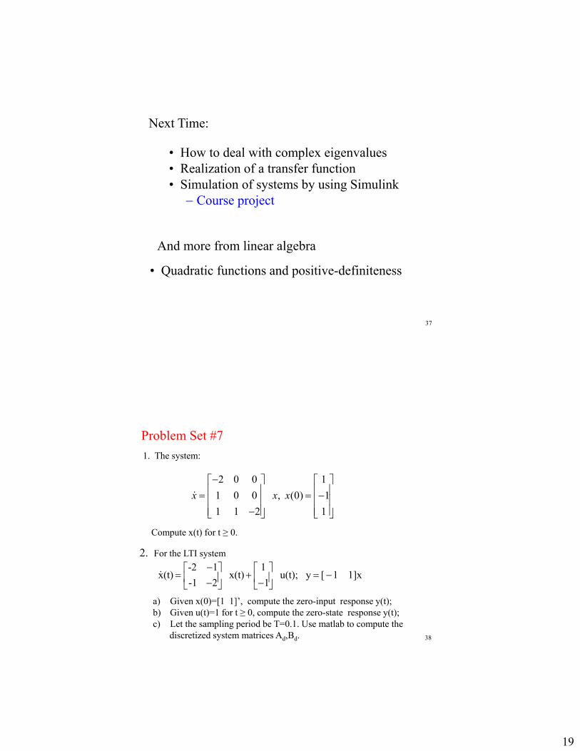
Next Time:

• How to deal with complex eigenvalues• Realization of a transfer function• Simulation of systems by using Simulink

Course project

And more from linear algebra

• Quadratic functions and positive-definiteness

38

Problem Set #7

1. The system:

2 0 0 1

1 0 0 , (0) 1

1 1 2 1

x x x

Compute x(t) for t ≥ 0.

-2 1 1x(t) x(t) u(t); y [ 1 1]x

-1 2 1

2. For the LTI system

a) Given x(0)=[1 1]’, compute the zero-input response y(t);b) Given u(t)=1 for t ≥ 0, compute the zero-state response y(t);c) Let the sampling period be T=0.1. Use matlab to compute the

discretized system matrices Ad,Bd.

20

39

Midterm Review (Lecture #1-Lecture #6)

Modeling of LTI systems Linear algebra

─ Vector spaces: LI, LD, basis, inner product, orthogonal─ Linear algebraic equation: range space, null space,

conditions for the existence of solution, all solutions─ Eigenvalues, eigenvectors, diagonal form─ Generalized eigenvectors, Jordan from─ Polynomial functions of a matrix─ eAt

40

Model of a circuit:• State variables?

– i1, i2, and v,

++

- - - u(t) R2 C

L1

+ y

L2 R1i1

v

• State and output equations?

1L1

1 vdt

diL

Cidt

dvC

21

22

2

22

111

1

11

iC

vi

C

1

dt

dv

vL

1i

L

R

dt

di

uL

1v

L

1i

L

R

dt

di

u

0

0L

1

v

i

i

0C

1

C

1L

1

L

R0

L

10

L

R

dt

dvdt

didt

di

1

2

1

22

2

11

1

2

1

i2

2L2

2 vdt

diL

v

i

i

0R0iRy 2

1

222

viRu 11

22iRv

21 ii

xx DuCxy

BuAxx

21

41

• What are the state variables?

• Select output of integrators as SVs

2

1/s 1/s+

-u(t)

y(t)

x1

x2

• What are the state and output equations?

21 xx

12 x2ux y = x2

u1

0

x

x

02

10

x

x

2

1

2

1

u0x

x10y

2

1

A B C D

12 xx

Integrators + amplifiers

42

Example

u2 y

+ +

++ 1/s1/s

1/s

a1

a2

a3

a4

u1 +

+

+

+

+

22

43

Elementary operations that preserve determinant

Elementary operations that preserve rank

Use elementary operation to transform a matrix into upper or lower triangular form

Linear Algebra Basics

44

Linear Independence

A set of vectors {x1, x2, .., xm} in Rn is LD if {1, 2, .., m} in R, not all zero, s.t.

1x1 + 2x2 + .. + m xm = 0 (*) If the only set of {i}i=1 to m s.t. the above holds is

1 = 2 = .. = m = 0then {xi}i=1 to m is said to be LI

Given {x1, x2, .., xm}, form 1 2 mA x x ... x

If A=0 has a unique solution, LI;If A=0 has nonunique solution, LD.

If rank(A)=m, the solution is unique LIIf rank(A)<m, the solution is not unique LD.

23

45

Examples: are the following sets of vectors LI, or LD?

,21,1

1,11 ,1,1 ,1

1,11 ,2,1

a

a

4,

3,2,

001

,3

,02,

001

ec

db

f

acba

310

,121

,011

,3

,02,

0

1cba

a

• LI if the rank of the matrix equals the number of columns

46

Basis and Representations• A set of LI vectors {e1, e2, .., en} of Rn is said to be a

basis of Rn if every vector in Rn can be expressed as a unique linear combination of them– For any x Rn, there exist unique {1, 2, .., n} s.t.

n

1iiinn2211 ee..eex

n

2

1

n21 :e...eex

n21 e...eex

– : Representation of x with respect to the basis

Theorem: In an n-dimensional vector space (or subspace), any set of n LI vectors qualifies as a basis

24

47

Change of basis:

;e...ee n21• Given a basis

• Let the new basis be:

Qe...eee...ee n21n21

• For x such that

βe...eex n21

βQe...eex 1n21

-We have

-1n21n21 Qe...eee...ee

Then,

48

– If (A) ([A : y]) (i.e., y R(A)), then the equations are inconsistent, and there is no solution

– If (A) = ([A : y]), then at least one solution

• If (A) = ([A : y]) < n (i.e., (A) > 0), then there are infinite number of solutions

• If (A) = ([A : y]) = n (i.e., (A) = 0), then there is a unique solution

─ For an nn matrix, Ax = y has a unique solution y Rm iff A-1 exists, or |A| 0

Linear algebraic equation Ax = y

25

49

Key concepts: Assume ARmn.

Range space R(A): {yRm: exists xRn s.t. y=Ax}• subspace of Rm, • dimension = (A), rank of A• basis: formed by the maximal number of LI

columns of ANull space N(A): {xRn: Ax=0}

• subspace of Rn,• dimension (A)=n-(A) • basis: formed by (A) LI solutions to Ax=0.

50

Example:

43 2 1 a a a a 100022104321

A

The range space R(A) is spanned by {a1,a2,a3,a4}What is the relationship among the vectors?What are (A), (A)? The dimension of R(A)? The basis of R(A)? The null spaces?

26

51

Parameterization of all solutions

Theorem: Given mn matrix A and a m1 vector y.─ Let xp be a solution to Ax = y. ─ Let (A)=k.─ Suppose k>0 and the null space is spanned by

{n1,n2,…nk}

The set of all solutions is given by {x = xp+1n1+2n2+…+knk: iR}

52

Eigenvalues, eigenvectors and diagonal form

Case 1: All eigenvalues are distinct

A scalar is called an eigenvalue of ACnn if a nonzero x Cn, such that Ax = x and x is the eigenvector associated with .

Theorem: the sets of eigenvectors {v1,v2,….,vn} is LI.Let Q=[v1 v2 … vn], then

n

2

1

1-

λ..00:::0..λ00..0λ

AQQ

27

53

Definition. A vector v is a generalized eigenvectorof grade k associated with if

,0vIA k

– What is the new representation w.r.t. {v1, v2, ., vk}? i.e.,

A[v1 v2 … vk] = [v1 v2 … vk]Ā

0vIAbut 1k

v, vDenote k ,vIAvIAv k1k

,vIAvIAv 1k2

2k

,vIAvIAv 21k

1

,0vIAvIA k1 11 vAv

212 vvAv

1k2k1k vvAv

k1kk vvAv

A Jordan block

……01 . …..

..00

1::

0..0

0..1

A

54

• Polynomial functions of a square matrix.

• Computation of eAt .

Today’s material will not be included in the midterm.

Questions?

28

55

Good luck!

Open book, open notes

Midterm exam: 6.30-9:30 pm, Oct 20 (Thursday)

No calculator, No Laptop