1644 ieee transactions on mobile …yuksem/my-papers/2017-tmc-2d...abstract—free-space-optical...

GPS-Free Maintenance of A Free-Space-OpticalLink Between Two Autonomous Mobiles

Mahmudur Khan,Member, IEEE, Murat Yuksel, Senior Member, IEEE,

and Garrett Winkelmaier,Member, IEEE

Abstract—Free-Space-Optical (FSO) communication has the potential to provide optical-level wireless communication speeds. It can

also help solve the wireless capacity problem experienced by the traditional RF-based technologies. Despite its capacity advantages,

FSO communication is prone to mobility. Since the FSO transceivers are highly directional, they require establishment and

maintenance of line-of-sight (LOS) between each other. We consider two autonomous mobile nodes, each with one FSO transceiver

mounted on a movable head capable of rotating 360 degree. We propose a novel scheme that deals with the problem of automatic

maintenance of LOS alignment between the two nodes with mechanical steering of the FSO transceivers. We design protocols to

maintain an FSO link between the mobiles satisfying a minimum received power or signal-to-noise ratio (SNR). We also present a

prototype implementation of such mobile node with FSO transceivers. The effectiveness of the alignment protocol is evaluated by

analyzing the results obtained from both simulations and also experiments conducted using the prototype. The results show that, by

using such mechanically steerable transceivers and a simple auto-alignment mechanism, it is possible to maintain optical wireless links

in a mobile setting with nominal disruption.

Index Terms—Free space optical communication, line of sight, autonomous mobiles, prototype

Ç

1 INTRODUCTION

FREE-SPACE-OPTICAL (FSO), a.k.a. optical wireless, com-munication has recently attracted significant interest

from telecommunication research and industry, mainly dueto the increasing capacity crunch faced by the radio fre-quency (RF) wireless technologies [2]. The heavily saturatedRF bandwidth is becoming more scarce as cellular capacityhas mostly hit its limits. FSO communication (FSOC) hasthe potential to complement the traditional RF networks. Ituses the unlicensed optical spectrum and mostly uses thesame basic optoelectronic technology as the fiber optic com-munications. FSOC can easily reach very high modulationspeeds (up to 10 Gbps [3]). Compared to RF, it can providemuch higher bandwidth channel to trasnfer large volumesof data. It can also provide connectivity in unfavorable con-ditions, e.g., presence of RF jamming or interception [4]. Ahighly useful feature of FSOC is its inherent signal securitydue to the containment of FSO signals behind walls andtheir low probability of interception and detection [5], [6].Also, high directionality of FSOC provides high spatialreuse and larger network capacity.

Applications of the existing FSO communication hasbeen mostly in immobile settings and at high altitudes (e.g.,space, satellite, building tops). Fixed FSOC techniques have

been studied to remedy small vibrations [7], swaying of thebuildings [8], interference and noise [9]. Line-of-sight (LOS)scanning, tracking and alignment have also been studiedfor years in satellite FSOCs [10], [11], [12]. These works con-sidered the use of mechanical auto-tracking [13], [14] orbeam steering [15]. There are also several scenarios involv-ing mobile nodes that can benefit from the various advan-tages offered by FSOC. Secure command and control ofmobile units in combat, sharing of high-resolution imageryand guidance data in next-generation air-traffic control, air-borne internet, and rapid communication deployment indisaster recovery are a few examples of these scenarios [16].

FSOC is very useful for signal security and RF challengedenvironments. So, equipping military robots like PackBotswith FSO/VLC (VLC stands for visible light communication)transceivers is a potential application area for FSOC. UsingFSOC/VLC with PackBots [17] instead of RF communicationcan prevent RF interception and jamming from enemies inwar zones. Another potential application of FSOC can beequipping robots like the NASA K10 robots [18] with suchtransceivers for Lunar/Mars exploration. Two K10 robots cancommunication with each other using FSOC at a lot morefaster speed than that using RF communication. UnmannedAerial Vehicles (UAVs) can also be equipped with such high-speed FSO/VLC transceivers that enables a large set of appli-cations involving transfers of very large wireless data [19].UAVs can be applied in both military or civil missions whichrequire many sensors and can generate large amounts of datato be transferred to other UAVs or a ground station. CurrentlyUAVs communicate through RF which offers a maximumcapacity of around 274 Mbps [20]. The higher data raterequired for communication links to transmit more informa-tion between UAVs can be provided by equipping themwithFSO/VLC transceivers.

� M. Khan and M. Yuksel are with the Department of Electrical and Com-puter Engineering, University of Central Florida, Orlando, FL 32816.E-mail: [email protected], [email protected].

� G. Winkelmaier is with the Department of Electrical and BiomedicalEngineering, University of Nevada, Reno, NV 89557.E-mail: [email protected].

Manuscript received 7 Dec. 2015; revised 27 July 2016; accepted 11 Aug.2016. Date of publication 25 Aug. 2016; date of current version 3 May 2017.For information on obtaining reprints of this article, please send e-mail to:[email protected], and reference the Digital Object Identifier below.Digital Object Identifier no. 10.1109/TMC.2016.2602834

1644 IEEE TRANSACTIONS ON MOBILE COMPUTING, VOL. 16, NO. 6, JUNE 2017

1536-1233� 2016 IEEE. Personal use is permitted, but republication/redistribution requires IEEE permission.See http://www.ieee.org/publications_standards/publications/rights/index.html for more information.

Despite the advantages over RF communication, the majorchallenge faced by FSOC is its vulnerability against mobility[2], [21]. Mobile FSOC requires effective maintenance of LOS.Since the optical beam is highly focused, the existence of LOSis not enough. The transmitter and the receiver must bealigned; and the alignmentmust bemaintained to compensatefor any sway or mobility in the nodes. In this paper, we pro-pose a novel scheme showing the feasibility of maintainingoptical wireless communication in amobile setting with mini-mal disruption using mechanically steered transceivers and asimple auto-alignment mechanism. We consider two autono-mous nodes/robots moving in random directions, each ini-tially unaware of the location of the other. We focus on thecase where the mobiles have an FSO transceiver each,mounted on a mechanically steerable head (which could aswell be a simple arm) capable of rotating 360 degree. In thispaper, we also present a prototype implementation of suchmobile FSOnodes.We show that using suchmechanical steer-ing capability to control the rotation of the transceivers, theproblem of LOS maintenance can be dealt with effectivelywithout global positioning system (GPS) but merely with an orien-tation device such as compass.

Maintaining a directional communication link would betrivial if a location service like GPS is available. However,for RF-challenged or indoor environments, solutions that donot utilize RF signals or GPS are needed. Within this con-text, our major contributions include:

� a theoretical framework for GPS-free maintenance ofFSO links so that calculation of mechanical steeringparameters (e.g., angular speed of the rotating arm)is feasible,

� a protocol for maintaining the FSO link at a desiredminimumSignal-to-Noise Ratio (SNR) or link quality,

� an approach that uses only the optical signals with-out any usage of RF signals for exchanging informa-tion among the mobiles, and

� an approach that does not need multiple transceiversor elements to detect the movement direction of theother mobile.

The rest of the paper is organized as follows: In Section 2,we review the literature for wireless link maintenancebetween multiple mobiles or in robot teams. Then, in Sec-tions 3, 4 and 5, we describe our proposed method for main-taining communication link between two autonomousmobiles using FSOC. Sections 6 and 7 presents a simulation-based evaluation of our approach. In Section 8 we describethe prototype in detail. In Section 8.1, we provide some initialexperimental results. Finally, we conclude in Section 9.

2 RELATED WORK

Maintaining wireless communication links between mobileshas been an attractive problem to both research and indus-try because of its desirability in many application areas,ranging from robotics to vehicular systems. In [22], FSOcommunication between two unmanned aerial systems(UASs) hovering in a given location and orientation is con-sidered. The authors developed a novel alignment modeland analyzed against simulated and multirotor platforms.In [23], the capabilities of a mechanical gimbal is investi-gated for use in a ground-to-UAV FSO communicationslink. In both of these works, laser transmitters are

considered and also either one or both nodes are stationary.while our work considers infrared VCSEL/LED transmit-ters, and communication between two mobile nodes.

A method for establishing a free-space optical-communi-cation link among nearby balloons with the aid of GPS, RF,camera, and communication with a ground station is pre-sented in [24]. In [25], a similar method is proposed thatuses predicted movement for maintaining optical-commu-nication lock with nearby ballons. In both [24] and [25], LOSalignment between the communicating nodes is firstachieved using GPS information or using a camera to local-ize the neighbor node. During this phase, RF communica-tion is used. Only after locating the neighbor node, apointing mechanism is used to align the FSO transceivers ofthe neighboring nodes. Then optical wireless communica-tion is used only for exchanging data. The optical wirelesslink is not used for maintaining the link.

A hybrid RF-FSO system is presented in [26], where, theauthors developed a system consisting of an MRR(Modulat-ing Retro-Reflector)-FSO link with a tracking optical terminal,a conventional RF link and a deployable pod to provide arelay node bridging the FSO link to the operator and the RFlink to the robot. This is a hybrid approach consisting of bothRF and FSO. Also the FSO communication is achieved usinglaser. Our approach consists pure optical wireless communi-cation, andwe consider LEDs andVCSELs as transmitters.

In terms of localizing and tracking, [27] presented experi-mental studies of strategies for maintaining end-to-end com-munication links for search-and-rescue and surveillance to abase station. The multi-robot team used in the experimentconsisted of four unmanned ground vehicles (UGVs) builtfrom radio-controlled scale model trucks each equipped witha laptop computer, odometry, stereo camera, GPS receiver,and a small embedded computer with 802.11b wireless con-nectivity, called the Junction Box (JBox). Likewise, Parkeret al. [28] deployed a team ofmobiles to form an indoor sensornetwork. In their approach the mobile sensors use differenttechniques such as acoustic sensing, laser scanning and avision system (such as, a camera) for localization. Shoval et al.[29] measured the relative position and orientation betweentwomobile robots using a dual binaural ultrasonic sensor sys-tem. Each robot was equipped with a sonar transmitter thatsends signals to two receivers mounted on the other robot. In[30], a laser-based pedestrian tracking system in outdoors ispresented using GPS-enabled mobile robots. In this trackingmethod, all the robots share the tracking data with each other,so that individual robots always recognize pedestrians thatare invisible to other robots.

Our approach considers absence of accoustic or ultrasonicsensing, vision system like camera, laser scanning, radio com-munication, and a central base station. It assumes FSOCbetween two mobile nodes, without any form of GPS, and onlyuses point-to-point distance measurement. We consider only FSOcommunication for both establishing/maintaining the link andexchanging information/data. It also assumes autonomy forthemobiles andworks in a completely distributedmanner.

3 TECHNICAL APPROACH

3.1 Problem Statement and Assumptions

For the problem of maintaining an FSO link between twomobiles, we make the following assumptions that the nodes:

KHAN ET AL.: GPS-FREE MAINTENANCE OF A FREE-SPACE-OPTICAL LINK BETWEEN TWO AUTONOMOUS MOBILES 1645

� are in a GPS-free environment with no medium ofcommunication available other than the FSO link;

� are mobile and completely autonomous;� move on both straight lines and curved lines;� are each equippedwith an Internal Measurement Unit

(IMU). The IMU consists of an accelerometer, gyro-scope and a compass/magnetometer giving them thesense of their own direction andmovement; and

� are each equipped with a mechanically steerablehead (with which they can scan the entire 360degree) that is mounted with a full-duplex FSOtransceiver.

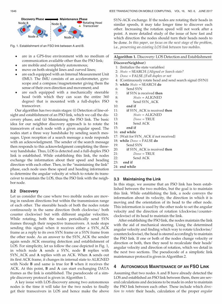
Our algorithm has twomain stages: (i) Detection of line-of-sight and establishment of an FSO link, which we call the dis-covery phase, and (ii) Maintaining the FSO link. The basicidea for our neighbor discovery approach is to rotate thetransceivers of each node with a given angular speed. Thenodes start a three way handshake by sending search mes-sages. Upon reception of a search message a node respondswith an acknowledgment. The sender of the search messagethen responds to this acknowledgment completing the three-way handshake. Thus, LOS is detected and a full-duplex FSOlink is established. While establishing this link, the nodesexchange the information about their speed and headingdirection with each other. Then, in the “maintaining the link”phase, each node uses these speed and heading informationto determine the angular velocity at which to rotate its trans-ceiver to maintain the LOS, thus the FSO link with the neigh-bor node.

3.2 Discovery

Let us consider the case where two mobile nodes are mov-ing in random directions but within the transmission rangeof each other. The steerable heads of both the nodes rotatecontinuously in the same direction (both clockwise/ bothcounter clockwise) but with different angular velocities.While rotating, both the nodes periodically send SYNframes through their respective transceivers. A node stopssending this signal when it receives either a SYN_ACKframe as a reply to its own SYN frame or a SYN frame fromthe other node. As an answer to the SYN_ACK the senderagain sends ACK ensuring detection and establishment ofLOS. For simplicity, let us follow the case depicted in Fig. 1,in which node A sends a SYN, node B replies withSYN_ACK and A replies with an ACK. When A sends outits first ACK frame, it changes its internal state to ALIGNEDwith Node B and same is true for B when it receives theACK. At this point, B and A can start exchanging DATAframes as the link is established. The pseudocode of a sim-ple discovery protocol is given in Algorithm 1.

A key issue with LOS discovery among two autonomousnodes is the time it will take for the two nodes to finallyget their transceivers in LOS and hence make the above

SYN-ACK exchange. If the nodes are rotating their heads insimilar speeds, it may take longer time to discover eachother. Increasing the rotation speed will not work after apoint. A more detailed study of the issue of how fast andwhich direction the nodes should turn their heads needs tobe done. In this paper, we focus on the next stage of the problem,i.e., preserving an existing LOS link between two mobiles.

Algorithm 1. Discovery: LOSDetection andEstablishment

DiscoverNeighbor()1: {Initialize the state variables}2: State = SEARCH //Aligned or Search state?3: Done = FALSE //Full duplex or not4: {Continuously rotate head and send search signal (SYN)}5: while State = SEARCH do6: Send SYN7: if SYN is received then8: State = ALIGNED9: Send SYN_ACK10: end if11: if SYN_ACK is received then12: State = ALIGNED13: Done = TRUE14: Send ACK15: end if16: end while17: {Wait for SYN_ACK if not received}18: whileDone = FALSE do19: Send SYN20: if SYN_ACK is received then21: Done = TRUE22: Send ACK23: end if24: end while

3.3 Maintaining the Link

In this stage, we assume that an FSO link has been estab-lished between the two mobiles, but the goal is to maintainthis link. While establishing the link, a node conveys theinformation about its velocity, the direction in which it ismoving and the orientation of its head to the other node.This information is used by the other node to set the angularvelocity and the direction of rotation (clockwise/counter-clockwise) of its head to maintain the link.

After establishing the FSO link, the nodesmaintain the linkwith the aid of mechanical steering. Using the determinedangular velocity and finding which way to rotate (clockwise/counterclockwise), the head is steered accordingly tomaintainthe FSO link. If one or both of the nodes change velocity ordirection or both, then they need to recalculate their heads’angular velocity and direction of rotation, which we detail inthe next two sections. The pseudocode of a simplistic linkmaintenance protocol is given inAlgorithm 2.

4 AUTONOMOUS MAINTENANCE OF AN FSO LINK

Assuming that two nodes A and B have already detected theLOS and established an FSO link between them, there are sev-eral calculations anddecisions to bemade in order tomaintainthe FSO link between each other. These include which direc-tion to rotate their heads, calculation of the proper angular

Fig. 1. Establishment of an FSO link between A and B.


velocity of the rotation, and calculation of the distance betweenthe nodes. Last but not the least, the nodes should know howfrequent and which specific information to exchange amongeach other so that the calculations and decisions could bemade in a timelymanner.We address these issues below.

Algorithm 2. Maintenance: Tune Angular Velocity of theHead

{Global variables}Dist Nodes //Distance between the two mobiles in metersRmax //Maximum communication range of the transceiver in meters{Head rotation variables}AngularVelocity //Degrees per secondAngularDirection //CW or CCW

{My movement/mobility variables}Velocity //My speed and direction of movementOrientation //Head’s orientation

{Neighbor’s movement/mobility variables}NVelocity //Neighbor’s speed and direction of movementNOrientation //Head’s orientation

{Periodically exchange velocity, direction & head orientation}{Called every tx seconds}ExchangeInfo()1: Send < Velocity; Orientation >2: Receive < NVelocity;NOrientation >{Periodically check the link and re-tune the angular velocity ofthe head}{Protocol A: Called every tx seconds}Maintain(amax)1: a ¼< Angle of Deviation > =u2: {Check if the link is still up}3: ifDist Nodes > Rmax then4: DiscoverNeighbor()5: else6: {Check if the link has deviated more than amax}7: if a > amax then8: Recalculate AngularVelocity9: Recalculate AngularDirection10: end if11: end if

4.1 The Angular Velocity: Three Cases

There are three cases according to the relative directions andpositions of the nodes. We detail these cases for

autonomously calculating the angular velocity of the nodes’heads so that the link can be maintained.

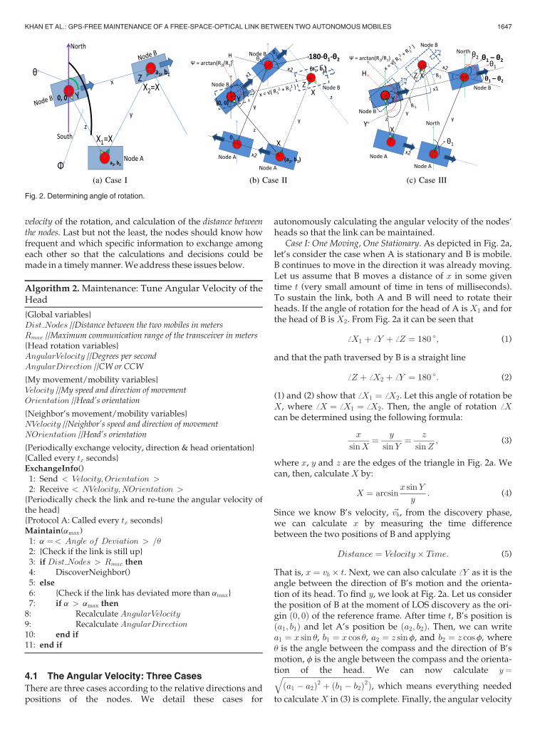
Case I: One Moving, One Stationary. As depicted in Fig. 2a,let’s consider the case when A is stationary and B is mobile.B continues to move in the direction it was already moving.Let us assume that B moves a distance of x in some giventime t (very small amount of time in tens of milliseconds).To sustain the link, both A and B will need to rotate theirheads. If the angle of rotation for the head of A isX1 and forthe head of B isX2. From Fig. 2a it can be seen that

ffX1 þ ffY þ ffZ ¼ 180 �; (1)

and that the path traversed by B is a straight line

ffZ þ ffX2 þ ffY ¼ 180 �: (2)

(1) and (2) show that ffX1 ¼ ffX2. Let this angle of rotation beX, where ffX ¼ ffX1 ¼ ffX2. Then, the angle of rotation ffXcan be determined using the following formula:

x

sinX¼ y

sinY¼ z

sinZ; (3)

where x, y and z are the edges of the triangle in Fig. 2a. Wecan, then, calculateX by:

X ¼ arcsinx sinY

y: (4)

Since we know B’s velocity, ~vb, from the discovery phase,we can calculate x by measuring the time differencebetween the two positions of B and applying

Distance ¼ Velocity� Time: (5)

That is, x ¼ vb � t. Next, we can also calculate ffY as it is theangle between the direction of B’s motion and the orienta-tion of its head. To find y, we look at Fig. 2a. Let us considerthe position of B at the moment of LOS discovery as the ori-gin ð0; 0Þ of the reference frame. After time t, B’s position isða1; b1Þ and let A’s position be ða2; b2Þ. Then, we can writea1 ¼ x sin u, b1 ¼ x cos u, a2 ¼ z sinf, and b2 ¼ z cosf, whereu is the angle between the compass and the direction of B’smotion, f is the angle between the compass and the orienta-tion of the head. We can now calculate y ¼ffiffiffiffiffiffiffiffiffiffiffiffiffiffiffiffiffiffiffiffiffiffiffiffiffiffiffiffiffiffiffiffiffiffiffiffiffiffiffiffiffiffiffiffiffiffiffiffiða1 � a2Þ2 þ ðb1 � b2Þ2Þ

q, which means everything needed

to calculateX in (3) is complete. Finally, the angular velocity

Fig. 2. Determining angle of rotation.


for A’s head will be ffX=t, since we know that

Angular Velocity ¼ Angular Displacement

Time: (6)

We will describe how to find z later in Section 4.2.Case II: One Node Eastbound, One Node Westbound. Fig. 2b

portrays another case where A is going westbound and Beastbound. Let u1 be the angle between the compass axisand the direction of motion of the first node, A and u2 be theangle between the compass axis and the direction of motionof the second node, B. Then, eastbound representsu2 ¼ ½0 �; 179 �� and westbound represents u1 ¼ ½180 �; 359 ��.Assume that B moves x1 and A moves x2 after discoveringLOS between each other. Similar to Case I, we can assumeA as stationary and B as moving with relative velocity~va þ ~vb which gives B’s relative displacement, x, as

~x ¼ ~x1 þ ð�~x2Þ. Here, x ¼ ffiffiffiffiffiffiffiffiffiffiffiffiffiffiffiffiffiR2

1 þR22

pand c ¼ arctanðR2=

R1Þ, where R1 ¼ x1 þ x2 cos ð180 � � u1 � u2Þ, R2 ¼ x2 sinð180 � � u1 � u2Þ, and c is the angle between the originaldirection and the relative direction of B’s motion. Similar toCase I, considering B’s position at the moment of LOS dis-covery as the origin ð0; 0Þ of the global reference frame, wecan calculate A’s position ða2; b2Þ at the moment of LOSdetection and B’s apparent position ða1; b1Þ at distance x.

This would give us y ¼ffiffiffiffiffiffiffiffiffiffiffiffiffiffiffiffiffiffiffiffiffiffiffiffiffiffiffiffiffiffiffiffiffiffiffiffiffiffiffiffiffiffiffiffiffiffiða1 � a2Þ2 þ ðb1 � b2Þ2

q. And ffY ¼

ffH � u2 � c. Here, ffH represents the orientation of thehead of Node B with respect to the compass axis. Finally,we then again use (3), (4), (5) and (6) to determine the angu-lar velocity, ffX=t.

Case III: Both Nodes Eastbound or Westbound. The last caseis portrayed in Fig. 2c, where A and B are both going east-bound, with velocities ~va and ~vb, respectively. Again, simi-larly to Case II, we can assume A as stationary and B asmoving with velocity ~vb � ~va. Here ~x ¼ ~x1 þ ð�~x2Þ, where

x ¼ffiffiffiffiffiffiffiffiffiffiffiffiffiffiffiffiffiR2

1 þR22

pand c ¼ arctanðR2=R1Þ. Here, R1 ¼ x1 � x2

cos ðu1 � u2Þ and R2 ¼ x2 sin ðu1 � u2Þ. Here, u1 ¼ anglebetween the compass axis and the direction of motion ofNode A. And u2 = angle between the compass axis and thedirection of motion of Node B. Similar calculations asin Cases I and II give us y. We then calculateffY ¼ ffH � u2 þ c. Finally, we apply (3), (4) and (5) and (6)to find the angular velocity, ffX=t.

These calculations for determining the angular velocityare applicable for nodes moving on both straight lines andcurves. We assume the curve to be a concatenation of a largenumber of very small straight lines. The distance x ¼ vbXtwould be very small since we assume t to be very small(10 ms� 1s). Although it is possible to further improve thiscalculation for curvature movements, we leave that forfuture work.

4.2 Determination of z

We represent the distance between the two mobile nodes atthe moment they discover the LOS as z. This distance (z) ismeasured only at the start of the maintenance phase. Tofind z, we assume availability of an optical distance mea-surement device, which are available in three categories:interferometry, time-of-flight (TOF) and triangulation meth-ods [31]. The FSO transceivers can use the TOF technique to

measure z. TOF refers to the time it takes for a pulse ofenergy to travel from its transmitter to an observed objectand then back to the receiver. If light is used as energysource, the relevant parameter involved in range countingis the speed of light, i.e., roughly 30 cm/ns. A TOF systemmeasures the round trip time (RTT) between a light pulseemission and the return of the pulse echo resulting from itsreflectance off an object. When LOS is established betweenthe two nodes, this technique is applicable.

Another method may be to measure the time betweensending a “Hello” packet to the neighbor and receiving aresponse for that packet. For this case, while calculating theRTT, we also need to consider the processing time ofthe receiving node (ms to ns) and transmission time of (ms)the control packet. We assume that processing time of thereceiver is constant and known to the sender or the process-ing time can be included in the response packet. The trans-mission time or time to insert the control packet into thepropagation medium can be calculated by dividing the sizeof the control message by the line rate (upto 155 Mbps [2]for VCSELS and LEDs). Since RTT is representative of trav-eling twice the distance and must therefore be halved tofind the actual range to the target [31]. In this case, RTT is

RTT ¼ trecv � tsend � tproc � ttrans; (7)

where, trecv is the time when response is received from thereceiver (Node B), tsend is the time when initial signal wassent by sender (Node A), tproc is the processing time of thenodes and ttrans is the time to insert the control packet intothe propagation medium.

4.3 Rotation: Clockwise (CW) or Counterclockwise(CCW)?

Another important decision to make for the nodes is whichway to rotate: clockwise or counterclockwise. Consideringtwo nodes A and B again, the decision depends on twoparameters: orientation of the heads and the direction ofmotion of the nodes. Fig. 3 depicts an example. Assume that,Node A was at location ð0; 0Þ and Node B was at locationða2; b2Þ at the start of the “Maintaining The Link” phase. Aftera given time, Node A moves to ða1; b1Þ and Node B Moves toða3; b3Þ. Here ffP is the orientation of the head of node A withrespect to the compass axis at the start of the “MaintainingThe Link” phase. ffQ is the orientation of the head of nodeA with respect to the compass axis after a given time.If ffP < ffQ, then rotation should be Counterclockwise.

Fig. 3. Rotation direction: Neighbor in northeast quadrant.


If ffP > ffQ, then rotation should be Clockwise and ifffP ¼ ffQ, there is no need for the nodes to rotate theirheads. Tables 1 and 2 show all the possible cases which aidsin deciding whether the rotation should be clockwise orcounterclockwise.

5 EXCHANGE PROTOCOLS TO MAINTAIN THE LINK

A crucial part of establishing the nodes’ autonomy is to letthe nodes decide how fast to turn their heads autonomously.We assume that the nodes will exchange their velocity andsignal quality values periodically over the FSO link itself.These periodic exchanges will allow the nodes to recalculatehow fast they should turn their heads so that the FSO linkstays up. We considered two different simplistic protocolsfor recalculating the angular velocity of the rotating head.

5.1 Protocol A: Maximum Angle of Deviation

Every time the nodes exchange their information, the receivernode will see if it has deviated greater than a preset threshold.If so, the receiver nodewill recalculate the angular speed of itshead.We assume that the nodes can turn their heads as fast asneeded, which is realistic since we only consider walkingspeeds.

Let tx be the time period of information exchangesbetween the two nodes. Further let a be the ratio betweenthe Angle of Deviation (ud) of the receiver from the the nor-mal of the other node’s beam and the Divergence Angle (u),and amax be the maximum allowed a before recalculation ofrotational speed is performed. At every tx, a is checked, andif a > amax then the angle of rotation (X) for the mobileFSO nodes are recalculated using (4), (5), (6).

During simulations, it was observed that ud >>Xwhen a > amax. So instead of updating X by directlyadding=subtracting ud, it is updated as follows:

ffX ¼ ffX 1� ud

u

� �: (8)

Also, a value of a > 1means that the link is down. Algo-rithm 2 lays down one particular implementation of Proto-col A as a pseudocode.

5.2 Protocol B: Minimum SNR

In this protocol, every time the nodes exchange their informa-tion, the receiver node will see if its received Signal-to-Noise

Ratio is less than a preset threshold. If so, the receiver nodewill recalculate the angular speed of its head. This design isparticularly useful if quality of the FSO link is important.

Let g be the difference (in dB) between the received SNRof the receiver and the receiver’s minimum required SNR,and gmin be the minimum allowed g before recalculation ofrotational speed is performed. At every tx, g is checked, andif g < gmin then the angle of rotation ðXÞ for the mobileFSO nodes are recalculated. A value of g < 0 means thatthe link is down. The angle of rotation is updated using (8).

6 SIMULATION SETUP

To gain insight into effectiveness of our approach, we per-formed simulations using MATLAB [32]. We consideredwalking speeds and reasonably capable robots for our nodes,e.g., Packbots [17]. We concentrated on the “Maintaining theLink” phase, and assumed that the nodes had discoveredeach other. We detail our simulation setup and assumptions,followed by results below. Table 3 lists the meanings of eachmathematical symbolwe used in ourmodels.

6.1 Transceiver Coverage Model

A key part of the simulation is to model transmission andfield-of-view areas of an FSO transceiver, which follow theLambertian law. To ease the computations, we approxi-mated an FSO transceiver’s coverage area L as the combina-tion of a triangle and a half circle, which was shown toapproximate the Lambertian coverage with a negligibleerror in [33]. Fig. 4 illustrates the key parameters: R, theheight of the triangle; u, the divergence angle and Rmax, themaximum reachable range. The radius of the half circle isR tan u, and R can be found by Rmax ¼ RþR tan u. Then,the coverage area of the transceiver, L, can be derived as

L ¼ R2 tan u þ 1

2pðR tan uÞ2: (9)

TABLE 1Neighbor in Northern Quadrants

Condition Rotation

ffP < ffQ CWffP > ffQ CCWffP ¼ ffQ None

TABLE 2Neighbor in Southern Quadrants

Condition Rotation

ffP < ffQ CCWffP > ffQ CWffP ¼ ffQ None

TABLE 3Mathematical Notations

Symbol Meaning

u Angle of Divergence (degrees)a Angle of Deviation / uamax Maximum allowed ag Received SNR - Minimum required SNR (dB)gmin Minimum allowed g (dB)tx Time period of information exchange(s)Nrec No. of RecalculationsRmax Maximum transmission range of transceiver (m)z Radius of receiver (cm)Pt Transmitter’s source power (dBm)S Receiver’s sensitivity (dBm)

Fig. 4. Coverage area of an FSO transceiver as “Triangle + Half Circle”.


The received power of an FSO transceiver is subject toLambertian loss due to radial distance from the axis of prop-agation (see Fig. 4), atmospheric attenuation and geometricattenuation [33]. The maximum communication range of anFSO transceiver is affected by these losses. The maximumrange Rmax that can be reached by an FSO transceiver (orthe maximum reachable range) is dependent on the trans-mitter’s source power P dBm, the receiver’s sensitivity SdBm, the radius of the transmitter b cm, the radius of thereceiver (on the other receiving FSO node) z cm, the diver-gence angle of transmitter u mRad, the visibility V km, andthe optical signal wavelength � nm. The maximum solutionof the following inequality gives us Rmax

�ðPt þ SÞ < 10log 10e�sR þ 10log 10

z

g þ 200Ru

� �2

: (10)

6.2 Divergence Angle

During our simulations, we tried different divergenceangles for the transceivers. We assumed that, for a trans-ceiver, both the transmitter’s divergence angle and thereceiver’s field-of-view are the same. Lasers operate with0.5 mRad (0.0286 degree) to 2.5 mRad (0.1432 degree) diver-gence angles, while VCSELs with 2.5 mRad (0.1432 degree)to 75 mRad (4.2972 degree) and LEDs with 60 mRad (3.4377degree) to 200 mRad (11.4592 degree) [33]. For our simula-tions, we considered VCSELs and LEDs as transmitters andconsidered 3, 5, 7.5, and 10 degree as divergence angles.

6.3 Minimum SNR in Protocol B

Protocol B aims to keep the quality of the FSO link above athreshold. The performance of a receiver degrades as aresult of several factors, including line-width, relative inten-sity noise (RIN) of the source, and receiver noise. Theseeffects have an impact on the maximum transmission dis-tance and signal coverage area. The performance of an opti-cal digital link is measured by the bit error rate (BER).Conversely, in an analog optical link, the performance ofthe receiver is measured by SNR. An example of such ananalog system is the optical wireless CATV system [34],where multiple analog or digital TV signals (or both) arecombined by means of subcarrier multiplexing (SCM) into asingle analog signal, which is then transmitted over an opti-cal link. To provide good picture quality, the analog signalmust have an SNR much greater than typical (e.g., 14 to 17dB) for non-return-to-zero (NRZ) signal. For analog TVchannels, the National Association of Broadcasters (NAB)recommends an SNR > 46 dB. For a digital TV channelwith QAM-256 modulation and forward error correction(FEC), a typical SNR > 30 dB is required [34], [35]. For oursimulation purposes, we chose the minimum required SNRof 30 dB for Protocol B.

6.4 Node Size and Configuration

Our main simulation scenario is to evaluate two Packbotsexploring a region of interest while maintaining an FSO linkbetween each other. So, we considered the nodes as Pack-bots having length and width of 75 cm and 40 cm respec-tively [17]. We considered a fixed value of Rmax (100 meters)for different values of the divergence angle. We consideredreceiver’s sensitivity of -43 dBm, visibility of 20 km, optical

signal wavelength of 1550 nm, transmitter radius of 0.3 cmand receiver radius of 3.75 cm. The required source powerfor the transmitter was calculated from (10).

6.5 Sensor Reading Errors

We consider both nodes to be equipped with an InternalMeasurement Unit (IMU) each. An IMU consists of an accel-erometer, gyroscope and a magnetometer. These sensors areused by the nodes to measure their own speed and headingdirection that they share with each other. These sensors aresensitive and contains measurement errors like noise, abias, scale factor error, g-sensitivity, cross-axis sensitivityetc. Disturbances in the magnetic field near the magnetome-ter can induce errors. This disturbances include power lines,motors, residual magnetism in the vehicle’s chassis etc. [36].We considered the presence of these errors in our simula-tions and associated different error values to the measure-ment of initial distance [31], speed [37] and heading [38] ofthe nodes. We denoted the different error values as follows:

� NE:No error was considered.� EC1: Error values between �0:25 m=s and 0:25 m=s

were randomly chosen from a truncated Gaussiandistribution and added to the speed measurement.

� EC2: Error values between �0:50 m=s and 0:50 m=swere added to the speed measurement.

� EC3: Error values between �0:75 m=s and 0:75 m=swere added to the speed measurement.

Moreover, for EC1, EC2 and EC3, error values between �3�

and 3� were added to the headingmeasurements and error val-ues between�0:25 m and 0:25 mwere added to the initial dis-tancemeasurements (determination of z) between the nodes.

7 SIMULATION RESULTS

We evaluated the performance of our approach using thetwo exchange Protocols A and B for recalculating the angleof rotation autonomously. We compare the percentage oftime the FSO link was down during our simulations. Weevaluated Protocols A and B under various ranges for theparameters shown in Table 3. We performed simulationsfor different values of the divergence angle u (2.5, 5, 7.5 and10 degree), amax (0.25, 0.5 and 0.75), gmin (5 dB, 6 dB, and7 dBb), and tx (10ms to 1s). We first considered Packbotsmoving on straight lines with speeds between 0m/s to2.5 m/s (or 9 km/h) [17]. We randomly chose the initialpositions of the nodes. We also randomly picked their initialspeed and heading direction for each simulation run. Foreach simulation run, after every two seconds, the speed ofthe nodes were increased by 10 percent of its current speedfor the first ten seconds. For the next ten seconds, the speedof the nodes were reduced by 10 percent of its currentspeed. If the link duration reached twenty seconds or if thenodes were out of each others’ communication range thesimulation was ended. For calculating the percentage oftime the link was down for each simulation run, we checkedevery 10 ms if a receiver node was within the coverage areaof the transmitting node, i.e., for protocol A we checked ifa > 1 and for protocol B we checked if g < 0. The valuesa > 1 and g < 0 were counted as misses. Dividing thecount of misses by the link duration value gave us thepercentage of link down value. For each parameter


combination, we calculated the average percentage of linkdown time and the number of message exchanges over 400simulation runs.

7.1 Using Protocol A

We simulated the protocol for different values of amax (0.25,0.5 and 0.75), and tx (10ms to 1s). In this section, we reportthe results where angle of deviation is used as the metric fordeciding when to re-tune the angular speed of the head’srotation (i.e., Protocol A). We simulated with two mobilityscenarios: (i) both nodes moving on straight lines and(ii) one node on a curve and the other on a straight line.

7.1.1 Both Nodes on Straight Lines

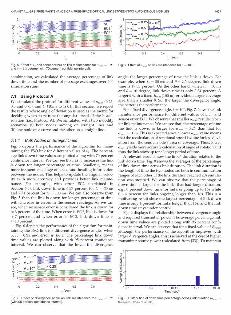
Fig. 5 depicts the performance of the algorithm for main-taining the FSO link for different values of tx. The percent-age link down time values are plotted along with 70 percentconfidence interval. We can see that, as tx increases the linkis down for longer percentage of time. Smaller tx meansmore frequent exchange of speed and heading informationbetween the nodes. This helps to update the angular veloc-ity with more accuracy and provides better link mainte-nance. For example, with error EC2 (explained inSection 6.5), link down time is 6.57 percent for tx ¼ 30 msand 7.71 percent for tx ¼ 100 ms. We can also observe fromFig. 5 that, the link is down for longer percentage of timewith increase in errors in the sensor readings. As we cansee, when no sensor error is considered the link is down for 5 percent of the time. When error is EC2, link is down for 7 percent and when error is EC3, link down time is 10 percent.

Fig. 6 depicts the performance of the algorithm for main-taining the FSO link for different divergence angles whenamax ¼ 0:25 and error is EC1. The percentage link downtime values are plotted along with 95 percent confidenceinterval. We can observe that the lower the divergence

angle, the larger percentage of time the link is down. Forexample, when tx ¼ 50 ms and u ¼ 2:5 degree, link downtime is 19.33 percent. On the other hand, when tx ¼ 50 msand u ¼ 10 degree, link down time is only 3.34 percent. Alarger u with a fixed Rmaxð100 mÞ provides a larger coveragearea than a smaller u. So, the larger the divergence angle,the better is the performance.

For a fixed divergence angle, u ¼ 10�, Fig. 7 shows the linkmaintenance performance for different values of amax andsensor errorEC1. We observe that smaller amax results in bet-ter link maintenance. We can see that, the percentage of timethe link is down, is larger for amax ¼ 0:25 than that foramax ¼ 0:75. This is expected since a lower amax value meansthat the recalculation of rotational speed is done for less devi-ation from the sender node’s area of coverage. Thus, loweramax yieldsmore accurate calculation of angle of rotation andthus the link stays up for a longer period of time.

A relevant issue is how the links’ duration relates to thelink down time. Fig. 8 shows the averages of the percentageof link down time across link duration. The link duration isthe length of time the two nodes are both in communicationranges of each other. If the link duration reached 20s simula-tion was stopped. We can observe that the percentage ofdown time is larger for the links that had longer duration,e.g., 0 percent down time for links ongoing up to 16s while0� 4 percent for links ongoing longer than 16s. This is amotivating result since the largest percentage of link downtime is only 4 percent for links longer than 16s, and the linkdown time stays under control.

Fig. 9 displays the relationship between divergence angleand required transmitter power. The average percentage linkdown time values are plotted along with 95 percent confi-dence interval. We can observe that for a fixed value of Rmax,although the performance of the algorithm improves withlarger divergence angles, this is achieved at the cost of highertransmitter source power (calculated from [33]). To maintain

Fig. 5. Effect of tx and sensor errors on link maintenance for amax ¼ 0:25and u ¼ 7:5 degree (with 70 percent confidence interval).

Fig. 6. Effect of divergence angle on link maintenance for amax ¼ 0:25(with 95 percent confidence interval).

Fig. 7. Effect of amax on link maintenance for u ¼ 100.

Fig. 8. Distribution of down time percentage across link duration ðamax ¼0:25; u ¼ 10o; tx ¼ 50 msÞ.


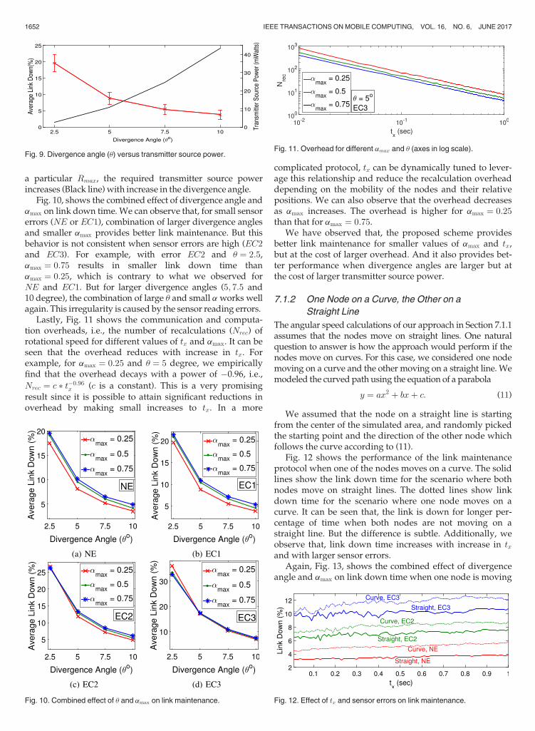
a particular Rmax, the required transmitter source powerincreases (Black line)with increase in the divergence angle.

Fig. 10, shows the combined effect of divergence angle andamax on link down time. We can observe that, for small sensorerrors (NE or EC1), combination of larger divergence anglesand smaller amax provides better link maintenance. But thisbehavior is not consistent when sensor errors are high (EC2and EC3). For example, with error EC2 and u ¼ 2:5,amax ¼ 0:75 results in smaller link down time thanamax ¼ 0:25, which is contrary to what we observed forNE and EC1. But for larger divergence angles (5; 7:5 and10 degree), the combination of large u and small aworks wellagain. This irregularity is caused by the sensor reading errors.

Lastly, Fig. 11 shows the communication and computa-tion overheads, i.e., the number of recalculations (Nrec) ofrotational speed for different values of tx and amax. It can beseen that the overhead reduces with increase in tx. Forexample, for amax ¼ 0:25 and u ¼ 5 degree, we empiricallyfind that the overhead decays with a power of �0.96, i.e.,

Nrec ¼ c t�0:96x (c is a constant). This is a very promising

result since it is possible to attain significant reductions inoverhead by making small increases to tx. In a more

complicated protocol, tx can be dynamically tuned to lever-age this relationship and reduce the recalculation overheaddepending on the mobility of the nodes and their relativepositions. We can also observe that the overhead decreasesas amax increases. The overhead is higher for amax ¼ 0:25than that for amax ¼ 0:75.

We have observed that, the proposed scheme providesbetter link maintenance for smaller values of amax and tx,but at the cost of larger overhead. And it also provides bet-ter performance when divergence angles are larger but atthe cost of larger transmitter source power.

7.1.2 One Node on a Curve, the Other on a

Straight Line

The angular speed calculations of our approach in Section 7.1.1assumes that the nodes move on straight lines. One naturalquestion to answer is how the approach would perform if thenodes move on curves. For this case, we considered one nodemoving on a curve and the other moving on a straight line. Wemodeled the curved path using the equation of a parabola

y ¼ ax2 þ bxþ c: (11)

We assumed that the node on a straight line is startingfrom the center of the simulated area, and randomly pickedthe starting point and the direction of the other node whichfollows the curve according to (11).

Fig. 12 shows the performance of the link maintenanceprotocol when one of the nodes moves on a curve. The solidlines show the link down time for the scenario where bothnodes move on straight lines. The dotted lines show linkdown time for the scenario where one node moves on acurve. It can be seen that, the link is down for longer per-centage of time when both nodes are not moving on astraight line. But the difference is subtle. Additionally, weobserve that, link down time increases with increase in txand with larger sensor errors.

Again, Fig. 13, shows the combined effect of divergenceangle and amax on link down time when one node is moving

Fig. 9. Divergence angle (u) versus transmitter source power.

Fig. 10. Combined effect of u and amax on link maintenance.

Fig. 11. Overhead for different amax and u (axes in log scale).

Fig. 12. Effect of tx and sensor errors on link maintenance.


on a curve. We again observe that, for no sensor errors (NE),combination of larger divergence angles and smaller amax

provides better link maintenance. But this behavior is notconsistent when sensor errors are present (EC1, EC2 andEC3). The combination of large u and small a works wellfor larger divergence angles (u > 2:5 degree for EC1, u > 5degree for EC2 and u > 7:5 degree for EC2).

7.2 Using Protocol B

In this section, we report the results where SNR is used as themetric for re-tuning (i.e., Protocol B). We again consideredwith twomobility scenarios: (i) both nodesmoving on straightlines and (ii) one node on a curve and the other on a straightline.We simulated this protocol also for different values of thedivergence angle, gmin (5dB, 6dB and 7dBb), and tx.

7.2.1 Both Nodes on Straight Lines

Fig. 14 depicts the performance of the algorithm for main-taining the FSO link for different values of tx using ProtocolB. Again, the percentage link down time values are plottedalong with 70 percent confidence interval. We can see that,

similar to the case using Protocol A, increase in tx causesthe link to be down for longer percentage of time. As dis-cussed earlier, smaller tx helps to update the angularvelocity with more accuracy and provides better link main-tenance. We can also observe from Fig. 14 that, the link isdown for longer percentage of time with increase in errorsin the sensor readings. As we can see, the link down time issmaller when there is no sensor error, compared to whensensor error is EC2 or EC3.

In Fig. 15, the effect of divergence angle of the trans-ceivers on link maintenance is shown when Protocol B isused for re-tuning the angular velocity of the node’s heads.Once again, we observe that, link maintenance is better per-formed with larger divergence angles.

For a fixed divergence angle, u ¼ 10 degree, Fig. 16 showsthe link maintenance performance for varying gmin. Weobserve that increasing gmin improves the performance.This is also an expected result because for a higher value ofgmin, the recalculation of angular speed is done for higherdifference between the receiver SNR and the thresholdSNR. Higher gmin means more accurate calculation of angleof rotation angle and thus better maintenance of the FSOlink is achieved.

Fig. 17 displays the combined effect of u and gmin, aver-aged over all possible values of tx. It can be seen thatincreasing the divergence angle yields better link mainte-nance. Also, increasing the gmin improves the performance.As we can observe, combination of a high divergence angle(u ¼ 10o) and a high gmin ¼ 7 dB, with error EC1, providesbetter ( 3 percent down time) link maintenance than that( 17 percent down time) obtained using a combination of(u ¼ 2:5 degree) and gmin ¼ 5 dB. Unlike the cases in proto-col A, increase in sensor error does not affect this largeu�high gmin combination.

Finally, Fig. 18 shows the communication and computa-tion overhead (i.e., the number of recalculations of rota-tional speed). Although higher gmin and smaller tx provides

Fig. 13. Combined effect of u and amax on link maintenance.

Fig. 14. Effect of tx and sensor errors on link maintenance forgmin ¼ 7 dB and u ¼ 10� (with 70 percent confidence interval).

Fig. 15. Effect of u on link maintenance for gmin ¼ 7 dB (with 95 percentconfidence interval).

Fig. 16. Effect of gmin on link maintenance for u ¼ 10 degree.


better link performance (Fig. 14), this is achieved at the costof higher overhead. Again we see that overhead reduceswith with increase in tx. So, it is possible to attain significantreductions in overhead by making small increases to tx.

7.2.2 One Node on a Curve, theOther on a Straight Line

We performed simulations using Protocol B also for the sce-nario where one node moves on a curve and the othermoves on a straight line. We again observe in Fig. 19 that,the link down time is slightly higher when one node is mov-ing on a curve compared to when both nodes are moving on

straight lines. Similar to the simulation results in Sections7.1.1, 7.1.2, and 7.2.1, we see that the FSO link is bettermaintained for smaller sensor errors. Also, the link mainte-nance is performed better with smaller tx (Fig. 19), largerdivergence angle, and higher gmin (Fig. 20).

8 PROOF-OF-CONCEPT PROTOTYPE

We designed and built a prototype of the mobile node witha mechanically steerable FSO transceiver by employingcommercially available off-the-shelf electronic components.The prototype and a block diagram of it are shown inFigs. 21 and 22, respectively. The main parts of the proto-type are: a robot car, a mechanically steerable head, a mag-netometer, and IR transceiver. All of these parts arecontrolled by a Raspberry Pi [39] using separate threads:head control, car control, compass readings, and transmitor receive data. Due to UART compatibility issues of Rasp-berry Pi, we added an Arduino [40] to handle the

Fig. 17. Combined effect of u and gmin on link maintenance.

Fig. 18. Overhead for different gmin and u (axes in log scale).

Fig. 19. Effect of tx and sensor errors on link maintenance.

Fig. 20. Combined effect of u and gmin on link maintenance.

Fig. 21. Bird’s eye view of the prototype.


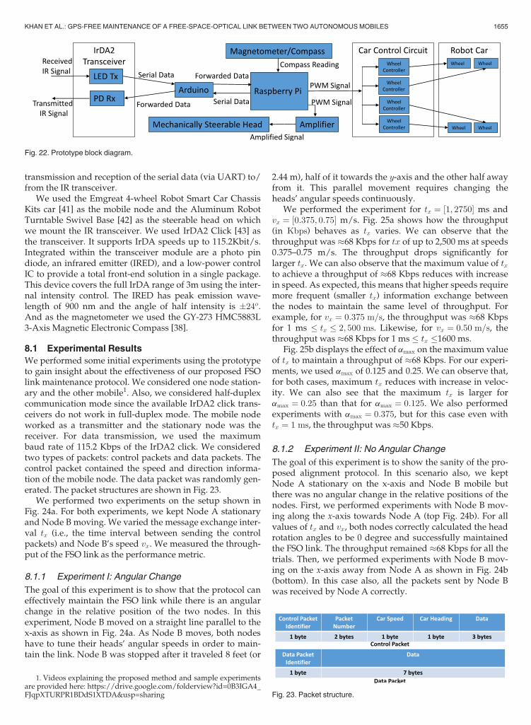
transmission and reception of the serial data (via UART) to/from the IR transceiver.

We used the Emgreat 4-wheel Robot Smart Car ChassisKits car [41] as the mobile node and the Aluminum RobotTurntable Swivel Base [42] as the steerable head on whichwe mount the IR transceiver. We used IrDA2 Click [43] asthe transceiver. It supports IrDA speeds up to 115.2Kbit/s.Integrated within the transceiver module are a photo pindiode, an infrared emitter (IRED), and a low-power controlIC to provide a total front-end solution in a single package.This device covers the full IrDA range of 3m using the inter-nal intensity control. The IRED has peak emission wave-length of 900 nm and the angle of half intensity is �24o.And as the magnetometer we used the GY-273 HMC5883L3-Axis Magnetic Electronic Compass [38].

8.1 Experimental Results

We performed some initial experiments using the prototypeto gain insight about the effectiveness of our proposed FSOlink maintenance protocol. We considered one node station-ary and the other mobile1. Also, we considered half-duplexcommunication mode since the available IrDA2 click trans-ceivers do not work in full-duplex mode. The mobile nodeworked as a transmitter and the stationary node was thereceiver. For data transmission, we used the maximumbaud rate of 115.2 Kbps of the IrDA2 click. We consideredtwo types of packets: control packets and data packets. Thecontrol packet contained the speed and direction informa-tion of the mobile node. The data packet was randomly gen-erated. The packet structures are shown in Fig. 23.

We performed two experiments on the setup shown inFig. 24a. For both experiments, we kept Node A stationaryand Node B moving. We varied the message exchange inter-val tx (i.e., the time interval between sending the controlpackets) and Node B’s speed vx. We measured the through-put of the FSO link as the performance metric.

8.1.1 Experiment I: Angular Change

The goal of this experiment is to show that the protocol caneffectively maintain the FSO link while there is an angularchange in the relative position of the two nodes. In thisexperiment, Node B moved on a straight line parallel to thex-axis as shown in Fig. 24a. As Node B moves, both nodeshave to tune their heads’ angular speeds in order to main-tain the link. Node B was stopped after it traveled 8 feet (or

2.44 m), half of it towards the y-axis and the other half awayfrom it. This parallel movement requires changing theheads’ angular speeds continuously.

We performed the experiment for tx ¼ ½1; 2750� ms andvx ¼ ½0:375; 0:75� m/s. Fig. 25a shows how the throughput(in Kbps) behaves as tx varies. We can observe that thethroughput was 68 Kbps for tx of up to 2,500 ms at speeds0.375–0.75 m/s. The throughput drops significantly forlarger tx. We can also observe that the maximum value of txto achieve a throughput of 68 Kbps reduces with increasein speed. As expected, this means that higher speeds requiremore frequent (smaller tx) information exchange betweenthe nodes to maintain the same level of throughput. Forexample, for vx ¼ 0:375 m=s, the throughput was 68 Kbpsfor 1 ms � tx � 2; 500 ms. Likewise, for vx ¼ 0:50 m=s, thethroughput was 68 Kbps for 1 ms � tx �1600 ms.

Fig. 25b displays the effect of amax on the maximum valueof tx to maintain a throughput of 68 Kbps. For our experi-ments, we used amax of 0.125 and 0.25. We can observe that,for both cases, maximum tx reduces with increase in veloc-ity. We can also see that the maximum tx is larger foramax ¼ 0:25 than that for amax ¼ 0:125. We also performedexperiments with amax ¼ 0:375, but for this case even withtx ¼ 1 ms, the throughput was 50 Kbps.

8.1.2 Experiment II: No Angular Change

The goal of this experiment is to show the sanity of the pro-posed alignment protocol. In this scenario also, we keptNode A stationary on the x-axis and Node B mobile butthere was no angular change in the relative positions of thenodes. First, we performed experiments with Node B mov-ing along the x-axis towards Node A (top Fig. 24b). For allvalues of tx and vx, both nodes correctly calculated the headrotation angles to be 0 degree and successfully maintainedthe FSO link. The throughput remained 68 Kbps for all thetrials. Then, we performed experiments with Node B mov-ing on the x-axis away from Node A as shown in Fig. 24b(bottom). In this case also, all the packets sent by Node Bwas received by Node A correctly.

Fig. 22. Prototype block diagram.

Fig. 23. Packet structure.

1. Videos explaining the proposed method and sample experimentsare provided here: https://drive.google.com/folderview?id=0B3IGA4_FJqpXTURPR1BDdS1XTDA&usp=sharing


9 SUMMARY AND FUTURE WORK

We presented a novel approach to overcome the problem ofmaintaining an FSO link between two autonomous mobilenodes. Each of the nodes is equipped with a mechanicallysteerable head (or arm) on which an FSO transceiver ismounted. Using the proposed algorithm to control themechanically steered head, the FSO transceivers on the nodescan maintain a communication link successfully. We outlinedall possible cases for calculating the angular velocity of thenodes’ heads and the direction of the heads’ rotation so as tomaintain the FSO link. We also presented two different proto-cols for deciding when to recalculate the angular velocity.One is based on the deviation of the receiver node from thetransmitter’s coverage area, the other based on a minimumreceived SNR.We also presented a prototype implementationof the abovementionedmobile FSO nodes. For evaluating ourproposed algorithm, we performed MATLAB simulationsand real experiments using the developed prototype. Weshowed through both simulation and experimental resultsthat, using a simple protocol to control themechanically steer-able head, the FSO transceivers on the nodes can maintain acommunication link successfully.

We assumed the height of the FSO transceivers to besame, i.e., we considered the nodes traveling at the sameheight. For nodes positioned at different heights or non-flatterrains, heads capable of rotating both in horizontal andvertical planes can be considered [19]. Nodes with fastertraveling speeds can also maintain FSO links using suchtransceivers as long as they are in each others’ communica-tion range for adequate duration of time. Also, we consid-ered FSOC between two mobile nodes. More future work isneeded to explore the scenarios involving more than twosuch nodes. Interference from multiple neighbor nodeswould be an interesting problem to tackle in this case.

In our prototype, the current communication speed is lim-ited by the IrDA2 Click (maximum 115.2 Kbps). This limitsthe speed of the data transfer between the nodes regardlessof the IR transceivers capabilities. Also, the maximum rangeof the IR transceiver is limited to three meters. Further, in theexperiments, we considered one stationary and one mobilenode with a half-duplex transceiver on each. To reap the fullpotential of the proposed FSO link maintenance protocol,full-duplex transceivers are required. As future work, weplan to develop full-duplex optical transceivers for improv-ing the prototype. The prototype can be further improved bycombining the circuits for the robot car, the mechanical head

and the transceiver in a single PCB board. Another possibleline of future work is to exploremulti-transceiver designs forthe mobile nodes. It is possible to equip each node with mul-tiple transmitters and/or receivers and use them for detect-ing the movement direction of the other node [2]. Suchredundancy will help both during the discovery andmainte-nance phases of our approach.

ACKNOWLEDGEMENTS

This work was supported in part by NSF awards 1321069and 1422354, ARO DURIP W911NF-14-1-0531, and NASASpace Grant NNX10A. During most of this work, theauthors were with the University of Nevada, Reno, NV89557. An earlier version of this work appeared in IEEEWCNC 2014 [1].

REFERENCES

[1] M. Khan and M. Yuksel, “Maintaining a free-space-optical com-munication link between two autonomous mobiles,” in Proc. IEEEWireless Commun. Netw. Conf., 2014, pp. 3154–3159.

[2] A. Sevincer, M. Bilgi, and M. Yuksel, “Automatic realignmentwith electronic steering of free-space-optical transceivers in MAN-ETs: A proof-of-concept prototype,” Ad Hoc Netw., vol. 11, no. 1,pp. 585–595, Jan. 2013.

[3] MRV optical communication systems, 2011. [Online]. Available:http://www.mrv.com/

[4] E. Leitgeb, J. Bregenzer, M. Gebhart, P. Fasser, and A. Merdonig,“Free space opticsbroadband wireless supplement to fiber net-works, in free-space laser communication technologies XV,” Proc.SPIE, vol. 4975, pp. 57–68, 2003.

[5] D. Zhou, P. G. LoPresti, and H. H. Refai, “Enlargement of beamcoverage in fso mobile network,” J. Lightw. Technol., vol. 29,pp. 1583–1589, 2011.

[6] S. Trisno, T.-H. Ho, S. D. Milner, and C. C. Davis, “Theoretical andexperimental characterization of omnidirectional optical links forfree space optical communications,” in Proc. IEEE Military Com-mun. Conf., 2004, vol. 3, pp. 1151–1157.

[7] S. Arnon and N. S. Kopeika, “Performance limitations of free-space optical communication satellite networks due to vibrations-analog case,” SPIE Opt. Eng., vol. 36, no. 1, pp. 175–182, Jan. 1997.

[8] S. Arnon, “Effects of atmospheric turbulence and building swayon optical wireless-communication systems,” OSA Opt. Lett.,vol. 28, no. 2, pp. 129–131, Jan. 2003.

[9] A. J. C. Moreira, R. T. Valadas, and A. M. O. Duarte, “Opticalinterference produced by artificial light,” ACM/Springer WirelessNetw., vol. 3, pp. 131–140, 1997.

[10] R. Gagliardi and S. KARP, “Optical Communications,” New York,NY, USA: Wiley, 1976.

[11] S. G. Lambert and W. L. Casey, Laser Communications in Space.Norwood, MA, USA: Artech House, 1995.

[12] S. Arnon and N. Kopeika, “Laser satellite communication net-work-vibration effect and possible solutions,” Proc. IEEE, vol. 85,no. 10, pp. 1646–1661, 1997.

Fig. 24. Experiment scenarios.

Fig. 25. Effect of tx and amax on throughput for different car speed.


[13] E. Bisaillon, et al., “Free-space optical link with spatial redun-dancy for misalignment tolerance,” IEEE Photonics Technol. Lett.,vol. 14, no. 2, pp. 242–244, Feb. 2002.

[14] M. Naruse, S. Yamamoto, and M. Ishikawa, “Real-time activealignment demonstration for free-space optical interconnections,”IEEE Photonics Technol. Lett., vol. 13, no. 11, pp. 1257–1259, Nov.2001.

[15] Y. E. Yenice and B. G. Evans, “Adaptive beam-size control schemefor ground-to-satellite optical communications,” SPIE Opt. Eng.,vol. 38, no. 11, pp. 1889–1895, Nov. 1999.

[16] D. Zhou, P. G. LoPresti, and H. H. Refai, “Evaluation of fiber-bun-dle based transmitter configurations with alignment control algo-rithm for mobile FSO nodes,” J. Lightw. Tech., vol. 31, pp. 249–356,2013.

[17] iRobot. (2015). [Online]. Available: http://www.irobot.com/us/learn/defense/packbot

[18] Nasa k10 robots. (2015). [Online]. Available: http://www.nasa.gov/centers/ames/K10/

[19] M. Khan and M. Yuksel, “Autonomous alignment of free-space-optical links between UAVs,” in Proc. 2nd Int. Workshop Hot TopicsWireless., 2015, pp. 36–40.

[20] D. Weatherington and U. Deputy, “Unmanned aircraft systemsroadmap, 2005–2030,” Deputy, UAV Planning Task Force, OUSD(AT&L), 2005.

[21] A. Ashok, M. Gruteser, N. Mandayam, J. Silva, M. Varga, and K.Dana, “Challenge: Mobile optical networks through visualmimo,” in Proc. MobiCom, 2010, pp. 105–112.

[22] A. Kaadan, D. Zhou, H. H. Refai, and P. G. LoPresti, “Modeling ofaerial-to-aerial short-distance free space optical links,” in Proc.IEEE Integr. Commun. Navigation Surveillance Conf., 2013, pp. 1–12.

[23] A. Harris, J. J. Sluss, H. H. Refai, and P. G. LoPresti, “Alignmentand tracking of a free-space optical communications link to aUAV,” in Proc. 24th Digital Avionics Syst. Conf., 2005, pp. 1–C.

[24] R. W. DeVaul, E. Teller, C. L. Biffle, and J. Weaver, “Establishingoptical-communication lock with nearby balloon,” US PatentApp. 13/346,645, Jan. 9, 2012.

[25] R. DeVaul, E. Teller, C. Biffle, and J. Weaver, “Using predictedmovement to maintain optical-communication lock with nearbyballoon,” US Patent App. 14/108,542, Dec. 17, 2013.

[26] J. L. Murphy, M. S. Ferraro, W. S. Rabinovich, P. G. Goetz, M. R.Suite, and S. H. Uecke, “Control of a small robot using a hybridoptical modulating retro-reflector/RF link,” Proc. SPIE, vol. 9080,2014, Art. no. -90 801F–12. [Online]. Available: http://dx.doi.org/10.1117/12.2052942

[27] M. A. Hsieh, A. Cowley, V. Kumar, and C. J. Taylor, “Networkconnectivity and performance in robot teams,” J. Field Robot.,vol. 25, pp. 111–131, 2008.

[28] L. E. Parker, B. Kannan, X. Fu, and Y. Tang, “Heterogeneousmobile sensor net deployment using robot herding and line-of-sight formations,” in Proc. IEEE/RSJ Int. Conf. Intell. Robots Syst.,2003, pp. 2488–2493.

[29] S. Shoval and J. Borenstein, “Measuring the relative position andorientation between two mobile robots with binaural sonar,” inPresented at the ANS 9th Int. Topical Meet. Robot. Remote Syst.,Seattle, Washington, 2001.

[30] M. Ozaki, M. Hashimoto, T. Yokoyama, and K. Takahashi, “Laser-based pedestrian tracking in outdoor environments by multiplerobots,” in Proc. 37th Annu. Conf. IEEE Ind. Electron. Soc., 2011,pp. 197–202.

[31] M.-C. Amann, T. Bosch, M. Lescure, R. Myllyla, and M. Rioux,“Laser ranging: A critical review of usual techniques for distancemeasurement,” Opt. Eng., vol. 40, no. 1, pp. 10–19, 2001.

[32] Matlab. (2015). [Online]. Available: http://www.mathworks.com/products/matlab/

[33] M. Yuksel, J. Akella, S. Kalyanaraman, and P. Dutta, “Free-space-optical mobile ad hoc networks: Auto-configurable buildingblocks,”Wireless Netw., vol. 15, no. 3, pp. 295–312, Apr. 2009.

[34] R. Ramirez-Iniguez, S. M. Idus, and Z. Sun, Optical Wireless Com-munications: IR for Wireless Connectivity. New York, NY, USA: CRCPress, 2008.

[35] W. Ciciora, J. Farmer, and D. Large, Modern Television Technology–Video, Voice and Data Communications. San Francisco, CA, USA:Morgan Kaufmann, 1999.

[36] E. Abbott and D. Powell, “Land-vehicle navigation using GPS,”Proc. IEEE, vol. 87, no. 1, pp. 145–162, Jan. 1999.

[37] H. H. Liu and G. K. Pang, “Accelerometer for mobile robot posi-tioning,” IEEE Trans. Ind. Appl., vol. 37, no. 3, pp. 812–819, Jun.2001.

[38] 3-axis digital compass ic hmc58831. (2015). [Online]. Available:https://www.parallax.com/downloads/hmc5883l-3-axis-digital-compass-ic-datash

[39] Raspberry pi. (2015). [Online]. Available: https://www.arduino.cc/en/reference/servo

[40] Ieik uno R3 board atmega328p. (2015). [Online]. Available: http://www.amazon.com/IEIK-Board-ATmega328P-Cable-Arduino/

[41] Emgreat 4-wheel robot smart car. (2015). [Online]. Available: http://www.amazon.com/Emgreat-4-wheel-Chassis-Encoder-Arduino/

[42] Aluminium robot turntable swivel base. (2015). [Online]. Available:http://www.ebay.com/itm/Aluminium-Robot-Turntable-Swivel-Base-2-DOF-PTZ-2pcs

[43] Irda2 click. (2015). [Online]. Available: http://www.mikroe.com/click/irda2/

Mahmudur Khan received the BSc degree inelectrical and electronic engineering from the Ban-gladeshUniversity of Engineering and Technology,in 2011 and the MS degree in computer scienceand engineering from the University of Nevada atReno (UNR), in 2015. He is currently workingtowards the PhD degree in the ECE Department atthe University of Central Florida. His research inter-ests include the area of free-space-optical commu-nications, wireless communications, and UAVcommunications. He is amember of the IEEE.

Murat Yuksel received the BS degree in com-puter engineering at Ege University, Izmir, Tur-key, in 1996, and the MS and PhD degrees incomputer science from RPI in 1999 and 2002,respectively. He is an associate professor in theECE Department at the University of CentralFlorida (UCF), Orlando, FL. Prior to UCF, he waswith the CSE Department at the University ofNevada—Reno (UNR), Reno, NV, as a facultymember until 2016. He was with the ECSEDepartment at the Rensselaer Polytechnic Insti-

tute (RPI), Troy, NY, as a postdoctoral associate and amember of adjunctfaculty until 2006. He worked as a software engineer at Pepperdata, Sun-nyvale, CA and a visiting researcher at AT&T Labs and Los AlamosNational Lab. His research interests are in the area of networked, wire-less, and computer systems with a recent focus on big-data networking,UAV networks, optical wireless, public safety communications, device-to-device protocols, economics of cyber-security and cybersharing, routingeconomics, network management, and network architectures. He hasbeen on the editorial board of Computer Networks, and published morethan 100 papers in peer-reviewed journals and conferences and is a co-recipient of the IEEE LANMAN 2008 Best Paper Award. He is a seniormember of the IEEE, and a senior and life member of the ACM.

Garrett Winkelmaier received the BS degree inelectrical engineering from the University ofNevada, Reno, in 2016. His research interestsinclude unmanned autonomous systems andmathematics. He is currently working withAboveNV as an engineer designing custom UAVsfor land surveying. He is amember of the IEEE.

" For more information on this or any other computing topic,please visit our Digital Library at www.computer.org/publications/dlib.


1644 ieee transactions on mobile …yuksem/my-papers/2017-tmc-2d...abstract—free-space-optical...

Documents