General rights Copyright and moral rights for the publications made accessible in the public portal are retained by the authors and/or other copyright owners and it is a condition of accessing publications that users recognise and abide by the legal requirements associated with these rights.

Users may download and print one copy of any publication from the public portal for the purpose of private study or research.

You may not further distribute the material or use it for any profit-making activity or commercial gain

You may freely distribute the URL identifying the publication in the public portal If you believe that this document breaches copyright please contact us providing details, and we will remove access to the work immediately and investigate your claim.

Downloaded from orbit.dtu.dk on: Feb 11, 2020

Climate Change Adaptation and Mitigation in Ecosystems - Benefits, Barriers andDecisionMaking

Møller, Lea Ravnkilde

Publication date:2016

Document VersionPublisher's PDF, also known as Version of record

Link back to DTU Orbit

Citation (APA):Møller, L. R. (2016). Climate Change Adaptation and Mitigation in Ecosystems - Benefits, Barriers and DecisionMaking. UNEP DTU Partnership.

Climate Change Adaptaon andMigaon in Ecosystems – Benefits, Barriers and Decision-Making

PhD DissertaonLea Ravnkilde MøllerNovember 2016

   

i  

 

 

 

 

 

 

   

   

ii  

PhD thesis        UNEP DTU Partnership    30 November11 2016 

Lea Ravnkilde Møller 

 

Author    Lea Ravnkilde Møller 

 

Title     Climate Change Adaptation and Mitigation in Ecosystems  

– Benefits, Barriers and Decision‐Making   

 

Supervisors  Anne Olhoff (principal supervisor) 

  Head of Programme, Climate Resilient Development   

UNEP DTU Partnership (UDP), Department of Management Engineering, Technical University of Denmark 

 

  Jette Bredahl Jacobsen (co‐supervisor) 

  Professor 

Department  of  Food  and  Resource  Economics,  and  the  Center  for Macroecology, Evolution and Climate,  

University of Copenhagen  

 

Financed by  UNEP DTU Partnership (UDP), Department of Management Engineering, Technical University of Denmark 

 

 

 

 

 

 

 

 

 

 

 

 

 

 

 

 

 

 

Front page: ‘Natural regeneration of mangrove forest’. Photo taken by the author in Peam Krasaop, 

Koh Kong Province, Cambodia, January 2014. 

 

   

iii  

                 

 

Preface  

This PhD thesis  is a result of my curiosity as to how synergies between climate change adaptation and mitigation can be achieved  in  the management of ecosystems, combined with my  fascination with getting lost in an ocean of data and making it tangible.    

The PhD thesis meets the requirements for the PhD degree at the Technical University of Denmark (DTU).  It  is  the  product  of  the  three‐year  PhD  programme  at  the UNEP DTU  Partnership  (UDP), Department  of  Management  Engineering,  DTU.  The  project  has  run  from  December  2011  to November 2016,  interrupted by  two maternity  leaves  from  January 2012  to December  2012  and from October 2014  to September 2015. The project has been supervised by Anne Olhoff, Head of Programme at the Climate Resilient Development, UDP, DTU, and Professor Jette Bredahl Jacobsen, Section  for  Environment  and  Natural  Resources,  Department  of  Food  and  Resource  Economics, University of Copenhagen. 

Essential  for  the  project  was  the  collaboration  with  Henrik Meilby  (University  of  Copenhagen), Santosh Rayamajhi  (Tribhuvan University, Nepal), Martin Drews  (DTU), Morten A. D. Larsen  (DTU), Jens Erik Lyngby (DHI), Tue K. Nielsen and other co‐authors. 

The thesis includes the following papers: 

Paper 1  Bakkegaard, R.K., Møller, L.R. & Bakhtiari, F. (2016). Joint Adaptation and Mitigation in  Agriculture  and  Forestry.  UDP  working  paper  series.  Climate  Resilient Development Programme. Working paper 2:2016.  

Paper 2  Møller,  L.R.  &  Jacobsen,  J.B.  (submitted  2016).  Estimating  the  Benefits  of  the Interrelationship between Climate Change Adaptation and Mitigation – A Case Study of Replanting Mangrove Forests in Cambodia. Scandinavian Forest Economics.  

Paper 3  Møller,  L.R.,  Smith‐Hall,  C.,  Larsen,  H.O., Meilby,  H.,  Nielsen,  Ø.J.,  Rayamajhi,  S., Herslund, L.B. & Byg, A. (manuscript to be submitted). Empirically Based Analysis of Households  Coping  with  Unexpected  Shocks  in  the  Central  Himalayas  Regional Environmental Change. 

Paper 4  Møller,  L.R., Drews, M. &  Larsen, M.A.D.  (submitted 2016). Simulation of Optimal Decision‐Making under the impacts of Climate Change. Environmental Management. 

 

   

   

iv  

Acknowledgements  

This PhD would not have been possible without the endless support of my husband Anders Jensen and our children Vilfred and Karla, to whom I dedicate this thesis in the hope that their future will be bright and that optimal decisions will be evident to them. 

I also owe many thanks to friends and family, especially my mother Lone Møller who has been very supportive  and  helped  with  the  family  logistics,  and  to  our  neighbours  Susanne  Nielsen,  Bente Østergaard Madsen  and  Nils  Boesen,  who  have  helped  us  in many  ways  and  contributed  with reflective discussions, offering perspectives on issues of development and constructive feedback. 

Next,  I  want  to  thank my  colleagues  at  the  UNEP  DTU  Partnership  for  fruitful  discussions  and constructive  feedback,  especially  Caroline  Schaer,  Sara  Lærke  Meltofte  Trærup,  Riyong  Kim Bakkegaard and Lars Christiansen  for  invitations  to coffee and  lunch breaks, addressing  the world situation  and  providing  encouraging  pep  talks  when  needed.  I  also  want  to  thank  peers  and colleagues at the University of Copenhagen for their hospitality during my research stay which made it a great learning experience that resulted in Paper 3 of this thesis.   

Furthermore, I want to thank the people of Peam Krasaop who allowed me to conduct fieldwork in their community, the project team behind the Cambodia Climate Change Alliance Programme, Jens Erik Lyngby from DHI and Tue Kell Nielsen for supportive information. A special thanks to Chea Leng and  Sun  Try, my  interpreter  and  chauffeur, whose  efforts made  the  fieldwork  possible.  Paper  2 would not have been possible had it not been for all of you. 

My dyslexia was of great concern to me before I started working on the PhD project, but with great support  from Roskilde Municipality, which made  it possible  for me  to hire professional assistance through Marie Lauritzen and Vision Editing, this was one thing that  I did not have to worry about. Their support has been an important part in my work on the thesis. Thank you. 

That  said,  there  would  not  have  been  a  thesis  to  submit  if  it  had  not  been  for my  two  great supervisors Anne Olhoff and Jette Bredahl Jacobsen, their willingness to answer my endless stream of questions regarding Matlab and STATA coding as well as their comments, clarifying questions and encouragement on rainy days. Thank you so much. It has been fun. 

 

   

   

v  

Popular Science Summary of the PhD Thesis, in English 

 

PhD student        Lea Ravnkilde Møller 

 

Title of the PhD thesis  Climate Change Adaptation and Mitigation in Ecosystems – Benefits, Barriers and Decision‐Making   

 

PhD school/department     UNEP DTU Partnership, DTU Management Engineering 

  

Science Summary 

Ecosystems are central to the livelihoods of many people and at the same time highly vulnerable to climate change. This  research, which  focuses on ecosystems and  land use,  investigates  linkages  in joint climate change adaptation and mitigation (JAM)  in ecosystems. The research exemplifies how different,  empirical  and  theoretical  models  for  decision‐making  can  be  applied  under  risk  and uncertainty, focusing on rural households  in developing countries. The thesis consists of four peer‐reviewed papers.  

The  first  paper  is  a  review  of  JAM  initiatives  in  the  forestry  and  agricultural  sectors,  highlighting current  barriers  and  opportunities  and  providing  insight  into  areas where  the  further  and  future development of  JAM  activities  can be ensured by  focused efforts.   The paper  concludes  that  the opportunities for achieving JAM are good, especially at landscape‐level.  

The  second  paper  analyses  the  economic  benefits  of  replanting  mangrove  forest  –  as  a  JAM initiative, simulated over a 100‐year period. The benefit of  this adaptation  initiative  is  reflected  in the avoided damage costs of storms. The benefits of climate change mitigation are estimated for the replanted area, i.e. a monetary value is projected based on different estimations of the social costs of  carbon.  The paper  concludes  that  combining  adaptation  and mitigation  can  improve  the  cost‐effectiveness of actions and increase their attractiveness to stakeholders and funding agencies.  

The  third paper  considers Nepalese households’ dependence on agricultural production and  their preferred coping strategies when faced with unexpected climate change shocks. A statistical model is  used  to  describe  the  households’  preferred  coping  strategies.  The  main  finding  is  that  poor households generally choose coping strategies that give them immediate access to cash as gap filler rather  than  income  and  resources  from  the  forests  and  the  environment  –  contrary  to  the assumptions of previous research. 

In  the  fourth  paper  a  framework  is  developed which  applies  Bayesian  updating within  decision‐making  in  a  forward‐looking  fashion.  The  focus  is  on  farmers’  choices  of  agricultural  system  as adaptation  to climate changes compared  to  their beliefs and  the  impact of  future climate change, simulating  the  consequences  of  farmers’  choices  of  adaptation  strategies  combined  with  their knowledge of climate change impacts for optimal decision‐making. 

The  overall  conclusion  of  this  PhD  project  is  that  combining  adaptation  and  mitigation  in  the agriculture  and  forestry  ecosystems  holds  significant  advantages  especially  from  a  landscape perspective. However, the  list of barriers  is  long, and therefore  it  is  important to acknowledge the links between adaptation, mitigation and development.   

 

   

   

vi  

Abstract  

Ecosystems are central to the livelihoods of many people and at the same time highly vulnerable to climate  change.  This  research,  which  focuses  on  ecosystems  and  land  use,  investigates  how households dependent on ecosystems can benefit from climate change adaptation and mitigation.  

Adaptation  and mitigation  are  two  different  approaches  to minimising  the  impact  and  extent  of climate change. The possible synergy between adaptation and mitigation is a topic that is currently attracting increasing attention, but which remains relatively understudied in the academic literature.    

The thesis consists of four peer‐reviewed papers, each of which considers a subject that contributes with increased knowledge as to how decision‐makers prioritise their choices to fight climate change, to  maximise  welfare  and  to  secure  better  decisions  when  facing  uncertainty  and  incomplete information.  

Paper 1  Joint Adaptation and Mitigation  in Agriculture and Forestry  takes a general approach  to synergies and  trade‐offs between adaptation and mitigation of climate change within  forestry and agriculture  in developing countries and considers previous experiences described  in  the  literature. The paper offers a summary of the described barriers and opportunities for achieving synergy. This is treated in more detail in each of the following papers: 

‐ Empirical  welfare  economic  benefits  of  climate  change  adaptation  leading  to mitigation (Paper  2.  Estimating  the  Benefits  of  the  Interrelationship  Between  Climate  Change Adaptation and Mitigation – A Case Study of Replanting Mangrove Forests in Cambodia) 

‐ Choice  of  coping  strategy  when  rural  households  dependent  on  agricultural  production experience  substantial,  unexpected  shocks  (Paper  3.  Empirically  Based  Analysis  of Households Coping with Unexpected Shocks in the Central Himalayas) 

‐ Simulation  of  decision  and  reaction  patterns  in  relation  to  the  belief  in  future  climate changes  and  trajectory  of  decisions  when  knowledge  about  future  climate  is  gradually increased  (Paper 4. Simulation of Optimal Decision‐Making under the  Impacts of Climate Change) 

Overall,  the PhD  thesis concludes  that  the opportunities  to achieve synergies between adaptation and  mitigation  of  climate  change  are  good,  especially  from  a  landscape  perspective.  Paper  1 concludes  that  there  is a need  for more empirical knowledge on  synergy, cost‐efficiency,  risk and uncertainty as well as the complexity of combining adaptation and mitigation. Joint adaptation and mitigation hold significant advantages especially from a landscape perspective. 

Paper  2  considers  such  empirical  knowledge  and  suggests how  incentives  to  increase  adaptation action can be achieved through carbon payments and a carbon credit scheme. Paper 2 highlights the importance of  considering  the  strategies  and options  for  tackling  climate  change,  and how  these may change over time. An important aspect hereof is the freedom of action and possible choices by those who  feel  the  impact  of  climate  change.  There  is  great  uncertainty  about  the  scale which increases the uncertainty about the actual benefits of adaptation and mitigation of climate change and complicates the process of deciding how to act.  

Paper  3  provides  a more  in‐depth  empirical  analysis  of  actual  decision‐making,  considering  rural Nepalese  households  dependent  on  agricultural  production.  Paper  3  finds  that  households  that experience substantial, unexpected shocks choose coping strategies that give them access to cash to 

   

vii  

overcome the shocks. Paper 4 exemplifies how freedom of action and optimal decisions can change over time, as knowledge increases.  

A  policy  recommendation  of  the  PhD  thesis  is  that when  striving  to  achieve  synergies  between climate change adaptation and mitigation  it  is necessary to understand that those who are hit the hardest typically are those with the  least resources. Thus, these people have  limited resources and freedom  of  action  to manage  possible  crises  and  do  not  have  resources  to  consider  long‐term strategies.  This  underlines  the  importance  of  linking  development with  the  fight  against  climate change  in order  to secure  increased  freedom of action  for  the world’s poorest,  thereby  increasing their ability to adapt and make optimal decisions for the future. Because climate change is a global issue, mitigation  should  be  included  in  decisions  to maximise  global welfare  and  the  PhD  thesis exemplifies situation of this.  

Summaries of the individual papers are available on page 23. 

   

   

viii  

Danish Summary – dansk resumé 

Denne afhandling tager udgangspunkt i muligheden for synergi mellem tilpasning til og reduktion af klimaændringer  i økosystemer med fokus på udviklingslande. Økosystemer er oftest yderst sårbare over  for  klimaændringer, hvilket gør de husstande, der er afhængige af økosystemerne, ekstremt sårbare.  Denne  afhandling  belyser,  hvordan  sådanne  husstande  vil  kunne  drage  nytte  af  en tilpasning til og en reduktion af klimaændringer, samt hvilke synergieffekter der kan opnås herved.  

Reduktion af og  tilpasning  til klimaændringer er  to  forskellige  tilgange  til at mindske omfanget og effekterne af klimaændringer. Synergi mellem reduktion og tilpasning er et emne, der tiltrækker sig øget opmærksomhed, men som stadig er relativt underbelyst i litteraturen.  

Afhandlingen består af fire artikler, der hver især omhandler et emne, der bidrager til øget viden om, hvordan  forskellige  beslutningstagere  bedst  prioriterer  indsatsen mod  klimaændringer  og  derved maksimerer  velfærden  og  træffer  bedre  valg  i  en  situation  med  usikkerhed  og  ufuldstændig information. 

Artikel 1  Joint Adaptation and Mitigation  in Agriculture and Forestry  tager en generel  tilgang  til synergierne mellem  tilpasning  til og reduktion af klimaændringer  inden  for skovbrug og  landbrug  i udviklingslande og ser på, hvilke erfaringer der er beskrevet  i  litteraturen. Artiklen opsummerer de beskrevne barrierer og muligheder for at skabe synergi. Dette bliver behandlet mere konkret i de tre efterfølgende artikler, der omhandler: 

‐ Empirisk,  velfærdsøkonomisk  estimering  af  nytten  ved  tilpasning  til  og  reduktion  af klimaændringer  (Artikel  2.  Estimating  the  Benefits  of  the  Interrelationship  Between Climate Change Adaptation and Mitigation – A Case Study of Replanting Mangrove Forests in Cambodia) 

‐ Beslutningsmuligheder og råderum for bønder i tilfælde af uforudsete klimarelaterede chok (Artikel 3. Empirically Based Analysis of Households Coping with Unexpected Shocks in the Central Himalayas) 

‐ Simulering  af  beslutnings‐  og  reaktionsmønstre  i  relation  til  troen  på  fremtidige klimaændringer og den udvikling, der sker i forbindelse med tilføring af ny viden om klimaets udvikling (Artikel 4. Simulation of Optimal Decision‐Making under the  Impacts of Climate Change) 

Overordnet konkluderer denne afhandling, at mulighederne for at opnå synergi mellem reduktion og tilpasning er gode,  især på  landskabsniveau. Artikel 1 konkluderer også, at det er nødvendigt med større empirisk viden om synergi, omkostningseffektivitet, usikkerhed og risici samt kompleksiteten ved at kombinere tilpasning til og reduktion af klimaændringer. Der er specielt gode muligheder for at  opnå  synergi mellem  tilpasning  og  reduktion  på  landskabsniveau.  Artikel  2  omhandler  netop denne empiriske viden. Artiklen viser, hvordan der kan opnås et  incitament  til øget  tilpasning ved udbetaling fra kulstof, svarende til de kreditter, der kan opnås i et kulstofkreditsystem. Derfor er det vigtigt  at  se  på  bredden  af  handlemuligheder  og  undersøge,  hvordan  strategierne  for handlemuligheder ændres over tid. Netop dette understreges  i den anden artikel. Råderummet og handlemulighederne  for  dem,  der  er  påvirket  af  klimaændringer,  er  et  vigtigt  aspekt,  fordi  der hersker stor usikkerhed om omfanget (påvirkningsgraden) af klimaændringerne og derved også stor usikkerhed omkring nytten  af  tilpasning  til og  reduktion  af  klimaændringerne. Dette  vanskeliggør beslutningsprocessen. Vigtigheden af dette bekræftes  i Artikel 3, hvor vi  ser, hvordan nepalesiske bønders valg  i tilfælde af uforudsete kriser er styret af muligheden for at få adgang til penge for at 

   

ix  

overvinde  krisen.  Artikel  4  eksemplificerer,  hvordan  optimale  valg  i  forbindelse  med  aktuelle råderum og handlemuligheder kan ændres, efterhånden som der opnås øget viden. 

De politiske anbefalinger i ph.d.‐afhandlingen er, at man ‐ for at skabe synergi mellem tilpasning til og reduktion af klimaændringer  ‐ er nødt til at forstå, at de, der rammes af klimaændringer, oftest har  de  færreste  ressourcer  og  derfor  rammes  ekstra  hårdt.  Dette  betyder  også,  at  de  har  et begrænset  råderum  til at klare sig  igennem eventuelle kriser og oftest  ikke har de  ressourcer, der skal  til  for  at  tænke  i  langsigtede  strategier. Dette  understreger  vigtigheden  af  at  sammenkæde udvikling med kampen mod klimaændringer  for på denne måde at  sikre verdens  fattigste et øget råderum. Det vil gavne deres  tilpasningsevne over  for klimaændringer og  sætte dem  i  stand  til at træffe bedre beslutninger for fremtiden. Da der er tale om et globalt problem, bør beslutninger om at  maksimere  velfærden  ved  en  reduktion  af  klimaændringer  træffes  på  globalt  plan,  og afhandlingen konkretiserer situationer, hvor dette vil give mening.   

 

Danish Summary of the Individual Papers ‐ dansk resumé af de enkelte artikler 

Artikel 1 (Joint Adaptation and Mitigation in Agriculture and Forestry) tager en overordnet tilgang til  tilpasningen  til og reduktionen af klimaændringer og ser på, hvilke erfaringer der er beskrevet  i litteraturen inden for skovbrug og landbrug i udviklingslande. Vi opsummerer de beskrevne barrierer og muligheder for at opnå synergi. Yderligere konkluderer artiklen, at synergi mellem reduktion og tilpasning  ikke  bør  tilstræbes  blot  for  at  gavne  begge,  men  at  den  mest  optimale  løsning  bør vurderes i hvert enkelt tilfælde ‐ lokalt og globalt. Artiklen understreger desuden vigtigheden af øget samarbejde mellem  lovgivende  institutioner  både  lokalt  og  globalt  for  at  skabe  synergi mellem klimatilpasninger og reducerede klimaændringer. 

Artikel 2 (Estimating the Benefits of the Interrelationship Between Climate Change Adaptation and Mitigation  –  A  Case  Study  of  Replanting Mangrove  Forests  in  Cambodia)  undersøger,  hvordan genplantning af mangroveskov kan være et middel  til klimatilpasning, der beskytter  fattige  fiskere bosat i området. Vi beregner tilpasningsgevinsterne ved at betragte de marginale, forventede, men hindrede skadesomkostninger for levevilkårene pr. genplantet hektar mangroveskov og gevinsterne ved  at  afværge  CO2‐binding  i  skoven.  Disse  to  potentielle  gevinster  sammenholdes  med etableringsomkostningerne for mangroveskov. Artiklen konkluderer, at ud fra et velfærdsøkonomisk perspektiv  så  er  nytten  ved  tilpasning  positiv  på  tværs  af  en  række  klimascenarier  og tilplantningsintensiteter. Denne virkning  forstærkes, hvis man  indregner gevinsten ved at reducere udledningen af drivhusgasser. Sidstnævnte vil føre til en højere grad af optimal tilplantning.  

Artikel 3 (Empirically Based Analysis of Households Coping with Unexpected Shocks in the Central Himalayas): På basis af data fra husstandsundersøgelser ser artiklen specifikt på, hvilke beslutninger nepalesiske  bønder  tager  for  at  komme  igennem perioder med uforudsete,  klimarelaterede  chok (positive eller negative), hvordan de tidligere har håndteret et klimarelateret tab eller en gevinst, og hvad de forventer at gøre, hvis en klimarelateret hændelse finder sted inden for det kommende år. Denne  analyse  anvendes  til  at  udforske,  hvilke  handlemuligheder  bønderne  har,  og  hvilke  de  vil vælge, hvis tabene som forventeligt bliver større i fremtiden på grund af klimaforandringer. Specifikt analyserer  vi  betydningen  af  deres  aktiver  (såsom  indkomst,  antal mænd  i  familien  og  husdyr)  i forhold  til  de  valg,  de  træffer,  ved  hjælp  af  en  ’multinomial  logit  regression’.  Resultaterne  af analysen er, at bøndernes  foretrukne  strategi  i  forbindelse med  tab er at  få hjælp  fra andre eller optage  lån.  I  forbindelse med  en  gevinst  vælger  de  hyppigst  opsparing.  Artiklen  konkluderer,  at bønderne oftest har et begrænset råderum til at komme igennem en krise, hvilket begrænser deres evne til at tilpasse sig fremtidige klimaændringer samt den nuværende klimavariabilitet.   

   

x  

Artikel  4  (Optimal Decision‐Making  – Adaptation  to  Climate  Change  in  the Agricultural  Sector) anvender  ’Bayesian  updating’  til  at  illustrere,  hvilke  handlemuligheder  man  har  i  forhold  til tilpasning,  og  hvilke  muligheder  der  er  for  at  modstå  fremtidige  klimaændringer.  Artiklen demonstrerer, hvordan det optimale valg kan ændre sig over tid, efterhånden som mere information bliver tilgængelig. Vi bruger et eksempel med repræsentative, ghanesiske  landmænd. Vi viser, at jo mere viden, der bliver tilgængelig over tid, jo bedre valg kan landmanden træffe. Dette viser værdien af at træffe beslutninger, som er fleksible, og som dermed kan tilpasses den usikkerhed, der ligger i klimaændringer. 

   

   

xi  

Table of Contents 

 

Preface            Acknowledgements          

Popular Science Summary of the PhD Thesis in English         Abstract              Danish Summary – dansk resumé     

Danish Summary of the Individual Papers ‐ dansk resumé af de enkelte artikler 

Table of Contents 

 

Part 1: Synopsis

 

1. Introduction                       1 

2. The Complexity of Climate Change Adaptation and Mitigation         3 

3. Research Objectives and Design                 5 

3.1 Research Objectives                  5 3.2 Delineation of Topics Covered by the Research           6 3.3 Research Design                   7 

4. Analytical Framework                   9  

4.1 Empirical Context ‐ Data Collection Methods and  Case Studies                     9 

Cambodia                   9   Nepal                   10   Ghana                   11 

4.2 Theoretical Approaches, Methods and Analyses         12 Paper 1: Literature Review of JAM           12 Method and Analysis               12 Discussion of Alternative Approaches           13 Paper 2: Estimating the Joint Benefit of  Adaptation and Mitigation             13 Method and Analysis               13 Discussion of Alternative Approaches           16 Paper 3: Multinomial Logit Regression for Analysis of Household  Resources Method and Analysis            18 Method and Analysis               19   Discussion of Alternative Approaches           19 Paper 4: Bayesian Updating ‐ An Adaptive  Approach to Management Decisions           20  Method and Analysis               21 Discussion of Alternative Approaches           22 

   

   

xii  

5. Extended Abstracts of the Papers               23  5.1 Paper 1                   23 5.2 Paper 2                   24 5.3 Paper 3                   25 5.4 Paper 4                   26 

6. Discussion                     28  

  6.1 Main Findings                 28 

6.2 Adaptation and Mitigation in an Ecosystem Services Perspective     29   

6.3 Linking Adaptation, Mitigation and Development         29 

6.4 Barriers to Decision‐Making               31 

7. Conclusion                     33 

   7.1 Further Research                  34 

8. References                     36       

 

Part 2: Papers 

 

Paper 1                       41   

Paper 2                       92 

Paper 3                     132 

Paper 4                     150 

   

   

1  

1. Introduction  

 

The main research objective of the PhD thesis is to explore the relationship between climate change 

mitigation and adaptation in ecosystems, focusing on barriers, opportunities and decision‐making at 

management unit  level. Ecosystems  are  central  to  the  livelihoods of many people,  and  some  are 

highly  vulnerable  to  climate  change.  It  is  generally  acknowledged  that  combining  adaptation  and 

mitigation  can  increase  the  effect  of  actions  (Chia  et  al.  2016; Mbow  et  al.  2014). However,  the 

existing conceptual and empirical knowledge base is too limited to fully assess such potential, and it 

is also questioned whether combining adaptation and mitigation is suboptimal (Duguma et al. 2014; 

Watkiss et al. 2015). Following the ratification of the Paris Agreement ‐ the first global agreement on 

climate change ‐ and the move towards its implementation, there are strong arguments in favour of 

increased  research  into  this  field.  Many  submissions  by  countries  (Nationally  Determined 

Contributions) specifically emphasise the linkages between mitigation and adaptation and the need 

to pursue mitigation, adaptation and development jointly. In addition, we are starting to see severe 

impacts  of  climate  change,  and  evidence  points  to  a  further  increased  impact  in magnitude  and 

scale. More  research  is  required  to  improve  our  understanding  of  ways  to  link  adaptation  and 

mitigation and of the possible benefits and optimal ways of doing so. The PhD thesis focuses on this 

issue of adaptation and mitigation in ecosystems.  

Ecosystems  refer  to  ecological  communities which  contribute  to  ecosystem  services  (Fisher  et  al. 

2009)  ‐  defined  as  the  benefits  that  people  and  communities  obtain  from  ecosystems  (UNISDR 

2009).  The  PhD  thesis  specifically  considers  situations  where  adaptation  and mitigation  can  be 

considered  as ecosystem  services  arising  from  ecosystem  impulses or ecosystem management  to 

deliver  the services  in an optimal manner. Ecosystem valuation  is a key element  in environmental 

decision‐making, making it possible to give ecosystem services a monetary value which can create a 

foundation for decisions (Fisher et al. 2009). The advantage of an ecosystem approach is that it gives 

us  the  freedom  to  look  at  interactions  between  ecosystem  complexity  and  structure  on  the  one 

hand and at people’s practices, values and regulation of ecosystems on the other (Termansen et al. 

2015). 

Sometimes it is not enough to know what the optimal response to climate change is. We also need 

to know whether  it  is possible  to make  the optimal decision, what conditions are  required  for  the 

optimal decision and who  is  taken  the decision. Optimal  responses will depend on what  is  found 

   

2  

desirable  for  the  future of  the  individual based upon  the existing  knowledge  level. The notion of 

capabilities  is central to decision‐making at farmer and household  levels.  Individual capabilities are 

determined by a person's freedoms of action, related to e.g. level of education, literacy and income 

level (Sen 2003). Low  levels of development will often be correlated with  low  levels of capabilities 

and can be a barrier to future  improved decision‐making on how to cope with or adapt to climate 

change. Capabilities can be increased through sustainable development. Sustainable development is 

intrinsically linked to adaptation, vulnerability reduction and enhanced climate change resilience and 

can be supported by local stakeholder involvement, acknowledging local knowledge – and scientific 

knowledge  –  in  a  learning  process  (Laukkonen  et  al.  2009).  It  is  therefore  important  to  consider 

relationships between adaptation and mitigation  in the context of decision‐making and sustainable 

development (Locatelli et al. 2015; Matocha et al. 2012; Watkiss et al. 2015).  

The following sections provide an overall framing for the research carried out under the PhD project 

and  the approaches and methods employed  in  the  four papers encompassed by  the PhD project. 

Section 1 is an introduction to the main research objective of combining climate change adaptation 

and mitigation  in ecosystems and  the  link  to development.  Section 2 discusses  the  complexity of 

climate change adaptation and mitigation, their differences and consistencies  in goals,  impacts and 

effects.  

Section 3 describes the overall and specific research objectives of the PhD thesis and how these have 

been  addressed.  This  is  followed  by  a  delineation  of  topics  covered  under  the  thesis  and  by  an 

account of the research design of the  individual papers, addressing the specific research objectives 

of the PhD thesis.  

Section 4 outlines the analytical framework, presents the empirical context of the individual papers 

and  considers  the applied  forms of data  collection and  case  study methods. This  is  followed by a 

presentation  of  the  theoretical  approaches, methods  and  analyses  applied  in  each  paper  and  a 

discussion of alternative methods that might have been used to achieve the research objectives.  

Section 5 provides an extended abstract of each of  the  four papers, while section 6 discusses  the 

main findings across the individual papers. Section 7 concludes the PhD thesis, including a discussion 

of the research contribution, interpretations of the contribution of scientific methods and empirical 

knowledge  and  the  possibilities  of  a  policy  implication  that may  facilitate  international  scientific 

consultancy and options for further research and perspectives. 

 

   

3  

2. The Complexity of Climate Change Adaptation and Mitigation 

 

The above introduction highlights the need for further research into climate change adaptation and 

mitigation and the possible disaster consequences if adaptation and mitigation are not achieved in a 

cost‐effective  manner.  It  also  highlights  the  need  to  gain  the  required  knowledge  about  the 

differences  and  consistencies  between  adaptation  and mitigation,  linking  it  to  development  and 

decision‐making. Thus, the complexity needs to be understood. 

The IPCC defines mitigation as an ‘anthropogenic intervention to reduce the sources or enhance the 

sinks of greenhouse gases’ (Klein et al. 2007). Adaptation is defined as an ‘[a]djustment in natural or 

human systems in response to actual or expected climatic stimuli or their effects, which moderates 

harm or exploits beneficial opportunities’ (Klein et al. 2007). 

Adaptation and mitigation differ at both  temporal and  spatial  scales, which  complicate  their  joint 

pursuit.  Firstly,  the  benefits of mitigation  are  typically  viewed  in  a  global,  long‐term perspective, 

given the time lag between greenhouse gas emission reductions and the achievement of equilibrium 

of  the concentration  in  the atmosphere. Furthermore, climate change  is a global  issue with public 

good  characteristics,  and  therefore,  it  does  not  matter  where  emission  reductions  or  sink 

enhancements  take  place  (Watkiss  et  al.  2015).  On  the  other  hand,  climate  change  adaptation 

contributes with disaster risk reduction and increased resilience and is therefore generally viewed at 

a local scale and in a short‐term perspective (Landauer et al. 2015; Watkiss et al. 2015).  

Secondly,  adaptation  and mitigation differ  in  terms of  the  actors who  are  involved. Mitigation  in 

ecosystems can be achieved through three main categories (Smith et al. 2014): reduction/prevention 

(conservation  of  existing  carbon  pools  to  avoid  emission  to  the  atmosphere),  sequestration 

(enhancing  the  carbon uptake  in  trees  and plants  in ecosystems,  thus  removing  carbon  from  the 

atmosphere  and  reducing  emissions)  and  substitution  (biological products used  as  substitutes  for 

fossil  fuels).  This  is  what  is  referred  to  as  the  supply  side  of  mitigation,  dependent  on  the 

management  behaviour. Mitigation  can  also  be  approached  from  the  demand  side,  considering 

changes in human lifestyle, behaviour, diet and consumption which are difficult to manage. This falls 

outside  the  scope  of  the  PhD  thesis. Mitigation  can  be  achieved  at many  different  levels:  from 

governments  and  national  institutions  trying  to  fulfil  their  national  commitments  to  the  Paris 

Agreement to private and individual stakeholders who recognise the business opportunities of new 

technologies or carbon payments.  

   

4  

Adaptation  can  also  involve different  levels of  institutions  and  actors  reacting  to  climate  change, 

either through planned or unplanned actions. Planned actions can be proactive, i.e. occurring before 

the  effects  of  climate  change  are  experienced,  or  reactive,  i.e.  occurring  after  changes  have 

occurred. Unplanned or autonomous adaptation to change (Tschakert &Dietrich 2010; Watkiss et al. 

2015) can be an unconscious response to changed conditions, thus improving the situation (Smit et 

al. 2001). Coping also  refers  to  reactive  responses  to climate change  impacts,  i.e.  initiatives which 

are based on the available resources and  implemented  in situations where shocks are unexpected 

and  short‐term,  immediate  reactions  are  necessary  to  overcome  the  situation  (UNISDR  2009). 

Coping is adaptation to a shock and how to get through a crisis, but does not minimise the long‐term 

effect of climate change as climate change adaptation.  

Considering adaptation and coping, there  is a risk that short‐term actions  implemented  in order to 

overcome  unexpected  shocks  increase  the  vulnerability  in  the medium  to  long‐term  perspective 

(Olhoff  &  Schaer  2010).  In  some  situations,  actions  necessary  to  cope  with  unexpected  shocks 

compromise  the  long‐term  perspective  of  adaptation.  Such  situations  can  be  defined  as 

maladaptation.  More  precisely,  maladaptation  is  defined  by  the  OECD  as  ‘business‐as‐usual 

development  which,  by  overlooking  climate  change  impacts,  inadvertently  increases  exposure 

and/or vulnerability to climate change. Maladaptation also includes actions undertaken to adapt to 

climate change impacts that do not succeed in reducing vulnerability but increase it instead’ (OECD 

2009).  

 

   

   

5  

3. Research Objectives and Design  

 

3.1 Research Objectives 

The main objective of  the  PhD  thesis  is  to  explore  and  assess  the  relationships between  climate 

change adaptation and mitigation  in  forestry and agriculture  in developing  countries with a main 

focus on barriers and decision‐making.  

The main objective  is addressed through the following three research focus areas,  including a brief 

summary of how the focus area in question is addressed in the thesis: 

I. Explore options for  joint benefits of climate change adaptation and mitigation, and 

how such benefits can be assessed.  

Prior  to  empirically  exploring  the  options  for  joint  benefits  of  climate  change 

adaptation and mitigation, Paper 1 contributes with a literature review and analysis 

of ways  in which mitigation  activities  can  generate  adaptation  benefits  and  vice 

versa. It also considers the integrated and synergetic effects that can be derived.  

Paper 2 contributes with an assessment of how benefits of JAM can be obtained. It 

includes a welfare economic analysis of the marginal economic benefits of replanting 

mangrove  forest  –  as  a  JAM  initiative  –  simulated  over  a  100‐year  period.  The 

benefits  of  adaptation  are  reflected  in  the  marginal,  avoided  damage  costs  of 

replanting an extra hectare. The marginal benefits of climate change mitigation are 

estimated  for  the  replanted  area.  A monetary  value  is  estimated  on  the  basis  of 

different estimations of carbon values – ranging from a likely price in the market to 

possible estimates of the social costs of carbon.  

 

II. Explore how decision‐makers make decisions  in order to cope with climate change, 

and how forward‐looking adaptation methodologies may improve such decisions. 

The  PhD  thesis  takes  two  approaches  to  investigating  the  second  research  focus. 

Paper 3 analyses agricultural production‐dependent Nepalese households’ preferred 

choices  of  coping  strategies  in  the  past  and  in  the  expected  future.  It  uses  a 

multinomial logit model to describe the households’ preferences of coping strategies.  

Paper  4  takes  a  forward‐looking  approach  through  Bayesian  updating.  The  paper 

presents  a  simulation  of  the  consequences  of  farmers’  choices  of  adaptation 

strategies  combined with  their  knowledge  of  climate  change  impacts  for  optimal 

   

6  

decision‐making.  Both  papers  discuss  the  options  to  improve  decisions  made  by 

decision‐makers. A  combination of  the  contributions of Papers 3 and 4 provides a 

perspective as to how the decision‐making can be  improved at a management unit 

level. 

 

III. Explore  current  barriers  to  implementation  of  climate  change  adaptation  and 

mitigation measures in forestry and agriculture, and how they can be overcome.   

The barriers are derived  from  the overview and analysis  in  the  four papers, which 

also discuss options to overcome these, e.g. the complexity of estimating the welfare 

benefits  of  local  adaptation  and  global mitigation  combined  (Paper  2),  and  rural 

households’  dependence  on  agriculture  and  their  choices  for  coping with  climate 

change, addressing the capacity barriers  in developing countries (Paper 3). Paper 4 

contains a  simulation of decision and  reaction patterns  in  relation  to  the belief  in 

future  climate  changes  and  a  trajectory  of  decisions when  the  knowledge  about 

future climate is gradually increased. 

 

3.2 Delineation of Topics Covered by the Research  

A main objective of the PhD thesis is to explore the management of ecosystems within the land use 

sector, focusing especially on agriculture and forestry and the links between these. Other key sectors 

for obtaining  JAM  include waste management, construction, planning and  infrastructure  (Illman et 

al. 2012), which, however,  fall outside  the  scope of  this  thesis. Similarly, governance and political 

decision‐making, bioenergy and migration are not included in the thesis, but play an important role 

for the choices of analyses  in the thesis. Hopefully, the thesis can contribute to  increased evidence 

of the situations where joint adaptation and mitigation should be pursued.  

Further discussion of the applied IPCC guidelines (IPCC 2006 and IPCC 2014) regarding calculation of 

the amount of carbon sequestrated through the replanting of mangrove forest and the possible risks 

and uncertainties of applying these methods also falls outside the scope of the thesis. The amount of 

carbon  sequestrated and emitted  for  replanting and destruction of mangrove  forest  in Paper 2  is 

calculated based on IPCC's guidelines.  

 

   

   

7  

3.3 Research Design  

Table 1 below provides a detailed outline of  the  research objectives and  the methods,  theoretical 

approaches, cases and examples applied in the four papers comprising the PhD thesis.   

Table 1 illustrates how research objectives I and II are divided between the four papers and how all 

four papers  contribute  to meeting  the  third  research objective  (III).  The  table  also  illustrates  the 

importance of decision analysis and its relation to climate change adaptation and mitigation.  

 

   

8  

Table 1 Interlinkages between the research objectives of the PhD thesis and the research questions and relations of the individual papers  Paper  Research 

objectives of the PhD thesis 

Research question(s) of the individual paper Methods Cases or examples Decision‐making analysed  

1  I + III  How does the literature define joint benefits between climate change adaptation and mitigation?   

What are the barriers to obtaining these benefits? 

Literature review of the underlying concepts of JAM.  

Applying a snowballing process to identify publications used and cited by others.   

Multiple examples drawn from existing literature regarding practices within agriculture and forestry in developing countries that create benefits for adaptation and mitigation. 

N/A

2  I + III  Does approaching adaptation and mitigation as complementary actions allow us to assess whether a combination of climate change adaptation and mitigation at a local case level can contribute to greater welfare compared to initiatives in which adaptation and mitigation are addressed separately in response to climate change?  

Explanatory interviews with households. 

Estimation of expected damage costs. 

Social cost of carbon. 

Replanting of mangrove forest in Peam Krasaop, Koh Kong Province, Cambodia. 

Analysis of the welfare benefits of joint adaptation and mitigation.   

3  II + III  Which coping responses have rural households utilised in the past to overcome unexpected shocks, and which coping responses do they expect to use in the future? 

How do households differ in their responses and how is this linked to their livelihood strategies and assets? 

 

Household surveys. 

Multinomial logit regression. 

Rural households level information on unexpected shocks, Mustang District, Nepal. 

PEN income survey. 

Analysis of rural households’ dependence on agricultural production choice as coping strategy in case of unexpected shocks (positive and negative). 

4  II + III  How fast should we adapt, or more precisely, when should farmers shift focus from one agricultural system to another to adapt to climate change? 

Bayesian updating.  

Climate realisation based on model combinations from the Coordinated Regional Climate Downscaling Experiment (CORDEX)  

Exemplifying Ghanaian farmers' choice of agricultural production as adaptation to climate change.  

The three climate scenarios: one global/regional climate model combination and two future scenarios (RCP4.5 and RCP8.5), representing the GHG reduction policy, moderate and unsustainable. 

Analysis of exemplified farmers’ choice of adaptation strategy and how it developed as the information of the future climate trajectory is revealed. 

 

   

9  

4. Analytical Framework  

 

The analytical and conceptual understandings of synergy between adaptation and mitigation and the 

important links to development, decision‐making, agriculture and forestry were outlined in sections 

1 and 2. The present section accounts for the empirical data (section 4.1) and the methodologies and 

theories applied (section 4.2) in the four papers to address the research questions and objectives of 

the individual papers.   

 

4.1 Empirical Context – Data Collection Methods and Case Studies 

The  following  sections  describe  the  empirical  examples,  cases  and  data  applied  in  the  individual 

papers. To a great extent, existing data is applied in the four papers. The countries used as cases and 

examples are developing countries found north of the equator. Paper 1 is a literature review and is 

therefore not considered in this specific section.  

 

Cambodia 

Exploratory  interviews  and  observations  were  conducted  by  me  in  Cambodia  from  January  to 

February  2014.  The  following  cities  and  rural  districts were  visited:  Phnom  Penh, Mondol  Seima 

District, Koh Kong Province and Prey Nob District, Sihanoukville Province, Cambodia. The purpose of 

the interviews was to get an overall impression and understanding of the living conditions of farmers 

and  fishermen  in  the  rural  districts  of  Cambodia.  Focus  was  on  the  two  projects  ‘Vulnerability 

Assessment and Adaptation Programme  for Climate Change within  the Coastal Zone of Cambodia 

Considering Livelihoods Improvement and Ecosystems’ (VAPP under the Least Developed Countries 

Fund (LDCF) project) and the ‘Coastal Adaptation and Resilience Planning Project’ (the CARP project), 

supporting  Cambodia’s  ‘National  Adaptation  Programmes  of  Action’  (NAPA)  strategy.  Partnering 

organisations  and  staff  at ministries  associated with  the projects were  interviewed  to obtain  key 

information  and  interviews  of  fishermen  and  farmers  implementing  integrated  farming.  Project 

documents and reports have been used to gain in‐depth knowledge about the CARP project and the 

cost  and  income  options  of  fishermen  in  Peam  Krasaop  (CCCA  2012).  The  CARP  project  is  being 

implemented alongside the longer running LDCF project. 

The Peam Krasaop community is located inside the Peam Krasaop Wildlife Sanctuary on the coast of 

Cambodia in the Koh Kong Province and is part of the CARP project. In October 2013, 15 hectares of 

   

10  

mangrove forest were replanted just outside the community border of Peam Krasaop ‐ as a climate 

change adaptation initiative.  

For simulation of wind damage caused by climate change and the ability of the mangroves to protect 

the  community  from  storm  damage,  historical  data  is  applied.  It  is  the  experience  that  damage 

occurs when the wind speed reaches 12 m/sec (CCCA 2012). Therefore, this has been referred to as 

a storm, even if it is not defined as such in technical terms. From 1979 to 2012, wind speeds over 12 

m/sec were measured at two points outside Cambodia's coast. These historical data have provided 

us with  an  opportunity  to  calculate  the  daily  probability  of  storms  for  each month  of  the  year 

(Nielsen 2013)  and  assess  the  community’s  vulnerability  to  climate  changes  and  cost of damages 

caused by wind  in 2011 (CCCA 2012). The data  is used to simulate day‐specific risk of wind speeds 

higher than 12 m/sec for a 100‐year period. Data from that CARP project and historical wind data are 

used as an empirical case in Paper 2.  

 

Nepal 

The data applied  in Paper 3 are  from Nepal,  focusing on  the Lete and Kunjo Village Development 

Committees  (VDCs  –  the  smallest,  local  administrative  unit  in  Nepal)  in  the  lower  part  of  the 

Mustang District  in  the Western Development Region of Nepal. Data originate  from  two different 

surveys, both of which were conducted from December 2008 to November 2009. The first stream of 

data consists of a time series of all environmental, farm and non‐farm income and asset data surveys 

originating from CIFOR’s Poverty Environment Network1 (PEN), following the PEN protocol (Angelsen 

et al. 2011; Larsen et al. 2014) (n=186). The second survey is a not previously published elaboration 

of the PEN survey, where household level information on unexpected shocks (negative or positive) is 

investigated. Data are obtained by asking the rural households about their behaviour in the past and 

their  expected  behaviour  in  the  future,  elaborating  on  affected  crop  types  in  the  agricultural 

production, the value of losses or gains and the expected standard value of the crop production that 

year, thus making  it possible to calculate the  lost or gained percentage and to specify whether the 

shock  in question was moderate  (< 50 per  cent) or  substantial  (> 50 per  cent). The  cause of  the 

losses or gains was also  registered as  closed‐ended questions. A  sequence of up  to  three  chosen 

coping  strategies  applied  by  the  households  in  case  of  unexpected  shocks  was  specified.  The 

households were also asked to specify how much a given coping strategy contributed to covering the 

unexpected loss or gain in production – within the range of 0‐20 per cent, 20‐80 per cent or 80‐100 

per  cent.  In  addition,  they  were  asked  to  assume  that  they  would  experience  a  substantial 

                                                       1 http://www.cifor.org/pen 

   

11  

unexpected  increase  or  loss  in  total  agricultural  production  in  the  coming  year  (moderate  or 

substantial). 

 A number of households were excluded as they did not complete all the  income surveys or could 

not be located at the time of interview (n= 112).  The survey is a subset sample of the PEN dataset. 

The two surveys were composed by Øystein Juul Nielsen and Santosh Rayamajhi, respectively. Paper 

3 contributes with a detailed description and the characteristics of the study area.  

 

Ghana 

Paper 4 uses Ghanaian farmers’ choices of agricultural systems as adaptation to climate change as 

an example of the behaviour of farmers. The basis is a representative farmer. The functions used to 

estimate  the  net  revenue  of Ghanaian  farmers’  income  from  the  three  agricultural  systems  are: 

dryland  crops,  irrigation  crops  and  livestock.  These  net  revenue  functions  originate  from 

Kurukulasuriya et al.  (2006). The  functions  contributing with  the marginal  climate  impacts on net 

farm revenues per farm (in USD) which are determined through a Ricardian model and ordinary least 

squares regression. The results of Kurukulasuriya et al. (2006) are based on more than 9,000 surveys 

conducted in 11 different countries. The coefficients applied for the net revenue functions are found 

to  be  biased  towards  irrigated  farming,  which  Kurukulasuriya  et  al.  (2006)  explain  as  an 

overrepresentation of data on  irrigated  farming  from Egypt, whereas  the  crop  in Ghana  is mostly 

rainfed. Therefore, we are not  just considering the mean coefficients, but also their minimum and 

maximum values for the net revenue functions. 

The main advantage of the data from Kurukulasuriya et al. (2006) is that the net revenues revealed 

by  their  analyses  reflect  the benefits  and  costs of  autonomous  adaptation  and  coping  strategies, 

such as the preference for more heat‐tolerant goats over cattle.  Autonomous adaptation includes a 

variety of contributions and the introduction of substitute actions, which farmers have incorporated 

in order to adapt to the current climate variabilities (Kurukulasuriya et al. 2006). 

 The  focus  of  Paper  4  is  to  show  how  the  farmers’  belief  in  climate  change  can  influence  the 

management decision. The exact results in quantitative terms are of less importance.  

The  second  data part of  Paper  4  is  a  detailed  analysis of  state‐of‐the‐art  regional  climate model 

projections  for  Ghana,  analysing  the  changes  in  inter‐annual  variations  of  temperature  and 

precipitation  in  chosen  climate  scenarios  and  trajectories  of  climate  realisations.  Paper  4  applies 

three climate scenarios to represent different, possible climate realisations, using precipitation and 

   

12  

(near  surface  air)  temperature  output  from  model  combinations  in  the  COordinated  Regional 

climate Downscaling EXperiment (CORDEX) database (Nikulin et al. 2012). 

The climate data is based on seven model combinations of output from where three global/regional 

climate model combinations and two future scenarios (RCP4.5 and RCP8.5), representing moderate 

and unsubstantial GHG reduction policies, respectively, were selected. The first scenario  is the RCA 

model, downscaling  the RCP4.5  scenario  (hereafter  titled C1)  to  constitute a  ‘baseline’  climate of 

minimal change. The second scenario (HIRHAM, RCP8.5 – titled C2) was chosen as it was wetter than 

most, representing a temperature increase in the lower range of the included models and exhibiting 

a positive temperature and precipitation. Conversely, the third scenario (MPI‐CCLM, RCP8.5 – titled 

C3) was  selected  for being  the driest, having  the highest  temperature  increase by  the end of  the 

century and a strong, negative temperature and precipitation correlation. 

 

4.2 Theoretical Approaches, Methods and Analyses 

The following provides an overview of the methods and analyses applied  in the different papers. It 

includes a discussion of why  these methods are applied and what alternative methods could have 

been selected. 

 

Paper 1: Literature Review of JAM 

In order  to  fulfil  the  research objective,  it  is necessary  first  to provide an overview of  the existing 

literature  on  JAM,  and  how  this  subject  has  previously  been  treated  within  the  ecosystem 

management  literature,  focusing on  land use sectors –  forestry and agriculture especially – with a 

large potential for JAM.  

 

Method and Analysis 

The  complex  connections between  climate  change  adaptation  and mitigation were  captured  in  a 

literature  review, which  applied  a  snowballing  process  to  identify publications used  and  cited by 

others. This approach was specifically chosen as a result of the  lack of consistently used keywords 

within  JAM  and  the  very  fragmented  literature.  The  literature  search was  conducted  during  the 

period  December  2015  to  March  2016.  The  starting  point  for  the  literature  search  was  peer‐

reviewed  papers,  however,  due  to  the  fragmentation  of  the  literature  also  grey  literature  was 

included. 

Paper 1  thus contributes with a necessary overview of  JAM. With  this  information  in hand,  it was 

possible to identify the research gaps and to use this knowledge to further develop the study area. 

   

13  

This study does not claim to be a complete review of all existing literature on the topic, as its focus 

has  been  on  forestry  and  agriculture.  However,  we  believe  that  the  study  covers  the  topic 

adequately  to provide an analysis of where  JAM can be  found within agriculture and  forestry, and 

also where the barriers to obtaining joint benefits are currently found. These findings shed light on 

new research directions that can contribute with new knowledge and fill in the research gaps in the 

fight against climate change.  

  

Discussion of Alternative Approaches 

Meta‐analysis might have been an alternative approach to conducting the  literature review of JAM 

in  the  land  use  sectors.  A meta‐analysis  enables  the  researcher  to  identify  and  gather  research 

findings  across  studies  that  examine  clearly  defined  subjects  through  identification  of  common 

effects.  Typically,  it  adopts  a  statistical  (meta‐regression  model)  approach  to  interpreting  and 

explaining  the  results  (Hunter & Schmidt 2004). However,  it was not possible  to  conduct a meta‐

analysis in Paper 1 as the literature on JAM is fragmented, the complexity of the subject high and the 

approach  to  the  subject  exploratory.  Existing  studies  do  not  have  adequate  information  and 

characteristics, and the current and general lack of empirical examples of JAM makes it impossible to 

treat the gathered information in a regression or similar, statistical analysis.   

 Paper 2: Estimating the Joint Benefits of Adaptation and Mitigation  

The main research question we wish to answer  in Paper 2  is whether a combination of adaptation 

and mitigation can lead to higher welfare. The focus of the paper is a marginal valuation of avoided, 

expected  damage  cost  (EDC)  and  the  possible  benefits  of  carbon  sequestration  from mangrove 

forest.  The  following  describes  how  EDC  may  be  used  to  estimate  the  value  of  the  potential 

contribution of ecosystems to joint adaptation and mitigation.   

 

Method and Analysis  

The approach takes the perspective of a social planner.  It assumes a utility function Ui(A,M,H,Z) of 

the services from an ecosystem under the impact of climate change in scenario i. U is a function of A, 

M and H, where A represents the benefits of climate change adaptation, M represents the benefits 

of climate change mitigation, and H represents the possible co‐benefits of combining adaptation and 

mitigation. Finally, Z  is the cost of enabling, establishing or  increasing the area of the ecosystem to 

contribute with mitigation and adaptation. If we allow U and the parameters within it to depend on 

time t, then the utility of the ecosystem services can be written as: 

   

14  

, , , ,       (1) 

where r is the discount rate, and subscript t denotes the time.  

Assuming that the utility is linear in input, we can write equation 1 as follows:  

, ,      (2) 

We assume that At, Mt and Ht are functions of the area of the entire ecosystem (St). This can e.g. be 

the  case where  the  ecosystem  has  erosion‐protective  or  carbon  sequestration  effects,  increasing 

with area size. We also assume that Z solely depends on the change of the size of the ecosystem (st) 

at time t.   Thus, we assume that the cost of changing the size of the ecosystem  is  independent of 

whether we  look at climate change mitigation or adaptation  initiatives. Thus,  if  the cost has been 

accounted for when estimating the benefits of adaptation, it is not necessary to account for the cost 

again when estimating the benefits of mitigation.  

The decision to be made  is how much of an ecosystem should be re‐established (st).  In Paper 2 we 

assume  that  the  re‐established  and  the  existing  ecosystems  have  the  same  value,  which  is  a 

reasonable  assumption  by  the  margin.  This  could  be  modelled  differently  if  the  health  of  the 

ecosystems, i.e. their ability to regenerate (Pramova & Locatelli 2013), was included explicitly in the 

valuation.  

We now look at how A and M can be estimated. The benefits achieved in addition to the benefits of 

adaptation  and mitigation  are  referred  to  as  co‐benefits  (H)  of  replanting mangrove  forest  (see 

Equation 1). H is assumed to be zero (Ht = 0) in the applied case of Paper 2.  

 

The Use of the Expected Damage Cost Approach to Estimating the Benefits of Adaptation (A) 

We estimate the increased welfare benefits of adaptation as the area increase (st) in relation to the 

ability  of  the  overall  area  (St)  to  contribute with  adaptation  of  climate  change.  This may  e.g.  be 

coastal  protection  as  in  Paper  2.  For  this  estimate,  we  need  to  look  at  the  expected  damage 

occurring for a given size of ecosystem. We do so by using the framework of an Expected Damage 

Function (EDF) based on Barbier (2007) and Hanley & Barbier (2009).  

The EDF has been used regularly in risk assessments and health economics looking at how changes in 

assets affect the probability of the occurrence of a damaging event. The method requires use of the 

ecosystem as  input, developing a ‘production function’ (Dupont 1991) for the ability of ecosystems 

   

15  

to adjust and  increase  the  resistance of  the community against  impacts  from climate change. The 

EDC is generally considered to be a valid approach to estimating the lower boundary of the value of 

avoided damage costs by mitigation of damages  (Boutwell & Westra 2015), as  it captures  the  full 

value of  an  ecosystem providing  a  service.  The  strength of  applying  the  EDC  is  that  it  allows  for 

careful evaluation of the assumptions behind it and thereby points out knowledge gaps. Boutwell & 

Westra (2015) highlight that errors may appear  if the case  is not well‐defined or the quality of the 

data is poor (Boutwell & Westra 2015). In Paper 2, the case is a well‐defined and very narrow – the 

case of Peam Krasaop in Cambodia. However, it is also a developing country context, where data is 

often  limited, as  is  the case here. Nevertheless, decisions are  still made – more or  less  informed. 

Consequently, judging the reliability of the assumptions is crucial, and possible caveats are discussed 

in Paper 2. Here the emphasis is on the setup. 

The expected cost of the damage is a measure of the welfare loss caused by changes in the minimum 

number of  acquired  goods  in  their  expenditure  function, which  again  is  a  result of  the  expected 

damage to the households due to climate change. This can be estimated as the minimum income for 

a  household  in  order  to maintain  the  utility  level  from  a  no‐change  scenario  in  a  given  climate 

scenario.  This  difference  is  called  the  compensating  surplus.  This  difference  in  utility  can  be 

expressed  as  a  marginal  willingness  to  pay  (USD/ha)  (the  expected  gain  from  changing  a 

wetland/mangrove  area  by  one  unit)  and  is  analogous  to  the  Hicksian  compensated  demand 

function for market goods (Freeman III et al. 2014). 

Discounting  and  aggregating  the  value  of  the  compensating  surplus  for  the  establishment  of  an 

ecosystem area can be calculated as the  integral of the reduced damage at all points  in time. This 

makes  it  possible  to  estimate  the marginal  value  (in  present  value  terms)  of  the  last  replanted 

hectare of mangrove forest in the context of climate change adaptation. It can be expressed as the 

marginal, avoided EDC. 

 

Estimating the Benefits of Mitigation (M) 

The underlying assumption of the ability of ecosystems to mitigate climate change is their ability to 

sequestrate CO2 from the air through plant growth and to capture it in organic material, e.g. wood, 

roots, dead organic matter. The benefits of mitigation may be calculated as the monetary value of 

the carbon sequestration  in the ecosystem at  time  t. As we have a social planner perspective, the 

monetary value can be seen as the social cost of carbon.  

   

16  

The benefits of mitigation at time Mt can be expressed as a function of  over the time period we 

are considering: 

                (3) 

Here L is the function for captured CO2 in the ecosystem. 

Aggregating and discounting over  time, we have  the contribution  to Equation 1, and  the marginal 

value of mitigation can be obtained  in a manner which for the  last established hectare  is similar to 

the marginal value of the avoided EDC.  

In Paper 2 the focus  is on replanting mangrove. Another example where the same approach could 

be used  is  the possible benefit of adaptation and mitigation  found through avoided deforestation. 

Deforestation (or clear cutting) can create an actual threat to a community due to an increased risk 

of  land  slides  and  flooding  combined  with  increased  precipitation  levels  from  climate  change 

(Matocha et al. 2012).  In that case A, M and Z from equation 2 could be defined as followed: A could 

be the benefit of adaptation, i.e. the economic value of the avoided damage to the community from 

landslides. M could be the benefits of mitigation, i.e. the amount of carbon stored above and below 

ground which  is at risk of being emitted to the atmosphere  in case of forest clearance. Z would be 

the  cost  per  hectare  of  avoided  deforestation,  i.e.  the  opportunity  cost,  and will  depend  on  the 

driver of the deforestation (e.g. deforestation caused by cattle farming or small scale slash‐and‐burn 

agriculture).  

 

Discussion of Alternative Approaches 

Considering  alternative  approaches  to  fulfilling  the  research  objective  of  Paper  2,  one  must 

remember the complexity of modelling the joint benefits of adaptation and mitigation. 

An alternative to the EDC approach is to consider the provision of A and M as a joint production2. In 

that case, the approach of Vincent and Binkley (1993) can be used, i.e. considering the production of 

two  goods  or  products  in  two  stands.  The  Production  Possibility  Frontier  (PPF)  summarises  the 

information regarding the benefits of the two products when sharing the management effort of the 

stands. Based on the classical theories of microeconomics with diminishing marginal return (Gravelle 

& Rees 2004),  it  is assumed  that  the PPF will be concave. However,  it may  take other  forms. The 

products  that Vincent and Binkley  (1993)  consider  are  timber  (T) and non‐timber  forest products 

                                                       2 A similar distinction is the concept of land sparing and land sharing. Here I choose to refer to joint production as it emphasises the value, as does the EDC approach. 

   

17  

(NT), two independent products. The production of T and NT is considered for two stands and jointly 

produced  in each  stand,  sharing  the management effort per hectare. They  show how  the  leading 

product can be superior to joint production by allocating the management effort to the product that 

does best under  the  specific  conditions of  the  stand. They highlight how products  can  contribute 

with a higher (economic or ecological) value.  

Joint production was not applied, as the production of adaptation and mitigation in the specific case 

of mangrove  replanting  is  not  a  trade‐off  between  the  two  objectives.  Carbon  sequestration  is 

inevitable when mangrove  is  replanted  for climate change adaptation. The marginal curve  for  the 

welfare benefits of adaptation and mitigation was estimated. This makes  it possible to  identify the 

optimal  level  for  replanting  mangrove  forest  in  three  climate  scenarios  and  two  replanting 

strategies.  These  scenarios  and  strategies  reflect  a  broad  range  of  results  and  visualise  the 

uncertainty which must be considered in future decision‐making. 

Vo  et  al.  (2012)  and  De  Groot  et  al.  (2002)  review  different  valuation  methods  for  mangrove 

ecosystems,  and  both  suggest  applying  avoided  cost  in  the  form  of  indirect market  pricing  as  a 

disturbance  regulator where  the ecosystems provide protection  from environmental disturbances. 

However,  avoided  cost  approaches  are  normally  static.  When  we  add  the  level  of  replanting 

scenarios  and  different  damage  regimes  from  climate  change  scenarios,  the  evaluation  becomes 

dynamic. Therefore, we further elaborate on it by applying the theory of the EDC (Hanley & Barbier 

2009).   

However,  it  is possible  to apply  joint production  in other cases where adaptation  is  included as a 

trade‐off for mitigation initiatives or vice versa. An example is a forest that contributes with timber 

production and protection  from soil erosion.  If  the harvest regime  is  increased,  the erosion of  the 

soil will increase and vice versa. Therefore, it is necessary to determine what has the highest priority. 

It is also possible to make the principle of joint production dynamic by discounting the different net 

revenues over time.   In the case of this PhD thesis it reflects how adaptation and mitigation benefits 

are most suitable across the landscape as a multi‐functional space (Scherr et al. 2012). 

If we had broadened the evaluation to also include the co‐benefits of replanting mangrove forest as 

mentioned above, this could have been  included by the preference‐based methods to capture e.g. 

non‐use values. However, as the case considered focuses on poor households, we consider it of less 

relevance to measure non‐use values.   

   

18  

The valuation of the mitigation benefits is expressed as an indirect use value that benefits society on 

a global  scale.  It originates  from  the  fact  that  forests  sequester  carbon. As mentioned,  the paper 

does not go  into details with  the accounting  rules, however,  it  is highly  relevant  to discuss which 

carbon prices should be applied. The results of Paper 2 clearly show that an increase in carbon prices 

changes the optimal level for replanting mangrove forest, increasing the benefits of adaptation. The 

paper  applies  carbon prices  in  the  range of USD 0.54 per  tCO2e  to USD 13.18 per  tCO2e. Critical 

voices are  likely to argue that we should apply a social cost of carbon (SCC) of about USD 200 per 

tCO2e. The SCC  is  the net present value of one more or one  less  tonne of CO2e emitted  (van den 

Bergh & Botzen 2015). SCC  is obtained from  integrated assessment models (IAM), but  it  is outside 

the scope of this PhD thesis to discuss the details hereof (see van den Bijgaart 2016, Tol 2008 and 

Nordhaus 2014, for a discussion of the topic).     

The argument for applying the low carbon prices was that they should reflect prices that could likely 

be  obtained  in  a market  for  quotas  and  thus  rely  on  the  political will  to  reach  agreements  that 

maximise  global  welfare.  An  optimal,  global  policy  would  lead  to  a  traded  carbon  price 

corresponding to the SSC. Paper 2, Appendix C, Figures C1 and C2, shows similar results as Figures 4 

and 5 in Paper 2, but with substantially higher carbon prices (CP1 = USD 50 per tCO2e, CP2 = USD 100 

per tCO2e, CP3 = USD 200 per tCO2e) with a discount rate of four and 12 per cent, respectively. What 

both  figures  show  is  that  regardless of  the damage  regime of  the different climate scenarios,  it  is 

beneficial to replant mangrove forest  in the case studied, and a higher carbon price makes  it even 

more  beneficial.  This  supports  the  original  conclusion  in  Paper  2  that  from  a  social  planner 

perspective,  there are benefits by replanting mangroves even when you only consider adaptation. 

The benefits are even higher when mitigation is included.  

The caveats stated in the paper are fully acknowledged. However, the above section argues in favour 

of the theoretical approach applied in Paper 2, which I believe to be well selected for the objective 

of the paper.  

 

Paper 3: Multinomial Logit Regression for Analyses of Household Resources  

The objective of the third paper is to increase existing knowledge about rural households dependent 

on  agricultural  production  and  their  choices  of  coping  strategies  when  faced  with  unexpected 

shocks, positive and negative, in the past as well as in the future. 

 

   

   

19  

Method and Analysis 

In Paper 3,  a multinomial  logit  (MNL)  regression  is  applied  to  analyse household  resources,  their 

choices of coping strategies  in the past and their expected future behaviour. When there are more 

than two choices, it is ‐ following the argumentation in Gebrehiwot & van der Veen (2013) ‐ correct 

to apply the multinomial regression model. For the specific study in Paper 3 of households’ choices 

of coping options, we estimated the likelihood of a certain choice characterised by a set of response 

variables. Thus we assume  that households’  responses are  rational and  that  they will  choose  the 

coping response that maximises their utility (McFadden 1973). The most preferred coping responses 

are used as the base category, as they are assumed to be available to all household types regardless 

of characteristics. The households’ resources are applied as explanatory variables. 

In this way it is possible to analyse the probabilities of the households’ choices of coping responses 

over the reference category compared to the households’ resources.  

 

Discussion of Alternative Approaches 

Alternative  approaches  to  the  data  analysis  method  of  Paper  3  include  a  hierarchical  MNL 

regression, able to handle the prioritisation of coping strategies which the households were asked to 

make  as  well  as  the  degree  to  which  the  coping  strategy  was  able  to  cover  the  loss  or  gain 

experienced by the household. It would presumably have required a larger dataset to maintain a fair 

degree of freedom.  

However, it might have been very interesting to apply the hierarchical MNL regression as this would 

allow  an  analysis  in  case  of  differences  between  the  'most  common'  and  'first  choice'  coping 

responses.  It  could  potentially  show  differentiation  between  coping  response  appearances,  e.g. 

where households would make a 'first choice' to cushion the impact of a shock and then later realise 

the  impact  and  apply  another  coping  response.    However,  in  the  MNL  model  there  were  no 

significant difference between moderate (< 50 % loss or gain) and substantial (> 50 %) shocks, so it is 

unlikely that there would be significant differences between 'most common' and 'first choice' coping 

responses in a hierarchical MNL regression. 

Another  issue  that might  have  been  interesting  to  capture  is  the  degree  to  which  households 

diversify their  income. In the survey this could have been  investigated by  looking at the number of 

crops species that the  individual household was growing, as this could  increase the resistance and 

ability to overcome shocks (cf. Branca et al. 2013; Jacobi et al. 2015; Linger 2014). This might also be 

considered as increased capabilities of the household and might have been investigated by means of 

   

20  

questions regarding adaptation (e.g. intercropping, wind breaks, agroforestry or having an orchard) 

and autonomous adaptation (e.g. change in crop species, increased irrigation, change in planting and 

sowing dates). However, these questions were not asked  in the survey. An  indication that  it might 

have been relevant is the fact that the MNL regression actually showed that households which spend 

money on  irrigation choose  to  reduce consumption  rather  than selling  livestock or  land or getting 

loans or assistance for coping with shocks (Table 6, Paper 3).  

Exploratory interviews might have been of huge interest in order to see how the households would 

reply  if  they were  asked  specifically  how  they would  react  to  a  devastating  natural  disaster  like 

earthquake or  landslides and they plan to spend the money saved from positive shock. Exploring  if 

the households’  reaction pattern and  coping  strategy would be different depending on  the  shock 

type they are hit by. The fear ‐ as in Wunder et al. (2014) – might be that the questionnaire does not 

capture  shocks  sufficiently  severe  to  capture  the  coping  strategies  that  really matter,  the  deep‐

uncertainty, high‐consequence, low‐probability events that can be devastating for a household. 

A conclusive question that needs to be asked in relation to this analysis is regarding people's ability 

to recall what they did five years back.   Rayamajhi et al. (2012) highlight that the ability of recall  is 

one of the limitations of quantitative forest income studies, as one‐year recall periods suffer from a 

serious underestimate of  forest  income  (Lund et al. 2008).   The  income survey applied  in Paper 3 

includes  annual  surveys  (at  survey  start  and  end)  and  four  quarterly  income  surveys  in  order  to 

accommodate  this  limitation.  The  second  part  of  the  data  set  applied  in  Paper  3  considers 

substantial and unexpected shocks which the households have experienced and which they must be 

expected to be able to recall ‐ otherwise they would not be substantial. There  is a small difference 

between  the households’ past and  future behaviour. A critical voice might  interpret  this as  if  they 

choose  to  remember  what  they  were  expected  to  do.  An  alternative  interpretation  is  that 

households  are  capable  of  critically  judging  how  they  got  through  past  shocks  and  consequently 

judging  how  they  expect  to  handle  future  shocks.  This  would  indicate  that  the  questionnaire 

exploring the households’ choices of coping is well defined for the past and the future. 

Based on  this evaluation of methods and approaches  for  the analysis  in Paper 3,  it  is  found well 

selected for Paper 3. 

 Paper 4: Bayesian Updating – An Adaptive Approach to Management Decisions 

Paper 4 deals with  the way  in which we make decisions and how we update  the decisions as we 

acquire new  information.  In  fact, we make subjective decisions about  the  future every single day. 

   

21  

When we  plant  trees  in  the  forest, we  assume  that  they will  be  able  to  survive  despite  climate 

change – if we consider climate change at all. If we buy a house by the coast, we evaluate whether 

the house will be affected by  rising  sea  levels during  the  time  that we will be  living  there. These 

decisions are irreversible in the short term due to the high costs associated with changing them, but 

they may  be  reversible  in  the  long  term  as we  gain more  knowledge  about  the  development  of 

climate  change.  If we  change our beliefs  concerning  climate  change, we will  likely plant different 

species.  If  new  information  emerges,  e.g.  new  flood  risk maps, we will make  different  decisions 

regarding housing. In Paper 4 we simulate this pattern of decision‐making based on our beliefs, and 

how the decisions may change as we gain more knowledge. Consequently, using Bayesian updating 

can simply be seen as a way of formalising decision‐making processes. It enables us to systematically 

analyse decisions and make  recommendations  that  reach  further  than decisions based on current 

beliefs. 

 

Method and Analysis 

We  apply  Bayesian  updating  of  beliefs  concerning  climate  change.  Basically,  a  set  of  subjective 

beliefs about  the  likelihood of various climate scenarios  is  identified. These may be based on past 

experience, on current observations, on rumours in society or on scientific evidence. Consequently, 

they may be considered to be subjective (Jacobsen et al. 2010). As time passes, a proactive decision‐

maker will observe the development of the climate (temperature and precipitation) and increase his 

knowledge of the realised climate scenario, changing the likelihood of the various climate scenarios, 

enabling  him  to  gradually  adapt  his  choices  in  order  to make  an  optimal  decision. Assuming  the 

decision‐maker makes  rational decisions, he updates  the beliefs of  the probability of outcomes – 

conditional  on  the  initial  belief.  Bayesian  updating  uses  Bayes’  theorem  (Bayes  and  Price  1763), 

which is given by (Equation 4):  

)(

)(AA

BP

APBPBP      (4) 

The equation states that  the probability of outcome A given another outcome B can be estimated 

based on the probability of B given A and the unconditional probabilities for each. In our setting, A is 

the probability of a given climate scenario and B  the current beliefs of probabilities. This makes  it 

possible to express a change in the probability as new data is observed (Skovgaard et al. 1999).  

 

   

22  

Discussion of Alternative Approaches 

The  ecosystem  services management  literature  on  estimation  of  future  optimal  decisions  adopts 

either  a  static  approach  (as  the  theory  of  joint  production  previously  described)  or  a  dynamic 

approach.  Bayesian  updating  belongs  to  the  dynamic  approach  which  takes  into  account  that 

conditions may change over time. 

Traditional  approaches  to  characterising  such  uncertainty  are  based  on  past  experiences.  This 

includes  e.g.  the  real  option  literature,  where  you  estimate  the  value  gained  from  additional 

information before making an irreversible investment (Arrow & Fischer 1974; Simal & Ortega 2011). 

Such  approaches  are  not  suitable  in  this  context  though,  because  they  are  based  on  known 

probability distributions which are not present when dealing with climate change (Yousefpour et al. 

2014). Using Bayesian optimisation makes  it possible to establish  if the optimal choice will differ  in 

accordance with the different beliefs  in climate change and realised climate change. However,  it  is 

not possible to identify the initially optimal decision. 

Applying  the  results  in Paper 4  to  the  applied Bayesian updating we  see  an example of how  the 

simulations reveal that the optimal choice actually does not change when using the mean coefficient 

from Kurukulasuriya et al. (2006) (Table 5, Paper 4), even when influenced by huge variabilities from 

the applied climate scenarios. The simulations show how the expected net revenue changes based 

on  the decision‐maker’s beliefs  in  the  future climate scenario, but  the optimal agricultural  system 

does not change. So even though the decision‐maker will not get the net revenue he expected based 

on his belief, the truth will prevail in this specific simulation.  

When applying the Bayesian updating, it is also interesting to reflect on the apparent 'nervousness' 

connected with  the choice of optimal agricultural systems, applying the minimum coefficient  from 

Kurukulasuriya et al. (2006) (Table 5, Paper 4).  Such vagueness is likely because of the variabilities in 

the climate scenarios, making  it difficult for the decision‐maker to  identify what climate scenario  is 

the  realised  one.   Here,  this  approach  gets  interesting  as  it means  that  it would  be  possible  to 

simulate the ambiguity of people's beliefs in climate change and the consequences hereof and at the 

same  time  simulate how  the decision‐maker’s  information of  the  realised  climate  increases,  thus 

enabling the decision‐maker to make the optimal choice ‐ something which is not possible applying 

in the real option theory.  

In  the  current  approach  we  have  assumed  a  risk  neutral  decision‐maker.  It  would  actually  be 

possible  to  include  risk  aversion  in  the  optimisation  process  within  the  Bayesian  updating 

framework, but we will leave this for future research.    

   

23  

5. Extended Abstracts of the Papers 

 

5.1 Paper 1 

Joint Adaptation and Mitigation in Agriculture and Forestry 

Authors: Riyong Kim Bakkegaard, Lea Ravnkilde Møller and Fatemeh Bakhtiari.   

UNEP DTU Partnership Working Paper series, Climate Resilient Development Programme, Working 

Paper 2: 2016.  

Keywords: Climate Change, Adaptation, Mitigation, Agriculture, Forestry. 

 

Introduction and Objective 

This working  paper  starts with  an  overview  of  the  underlying  concepts  of  joint  adaptation  and 

mitigation  (JAM).  It  captures  how  literature  has  defined  the  concept  as  benefits,  synergies, 

integration,  interlinkages  and  interrelationships  and  analyses  of  how  mitigation  activities  can 

generate adaptation benefits and vice versa, and which synergetic effects might be derived from the 

pursuit of  joint activities  in the forestry and agricultural sectors. This  is  illustrated by practices and 

actions in agriculture and forestry in developing countries which are creating benefits for adaptation 

and mitigation.  

 

Main Findings and Contributions 

The paper outlines current barriers and opportunities for the pursuit of JAM within agriculture and 

forestry, offering guidance on where efforts should be focused to ensure the future development of 

JAM activities. These can among others include institutional and capacity barriers and opportunities, 

knowledge barriers and, importantly, funding barriers and opportunities.  

For  example,  the  historical  and  traditional  way  of  separating  adaptation  and mitigation  creates 

barriers  at  institutional  and  governance  levels.  The  lack  of  adequate  metrics  for  measuring 

adaptation is also a major barrier to the success of joint activities and to the further development of 

JAM  activities.  Likewise,  the  lack  of  funding  is  a  barrier  to  both  adaptation  and mitigation.  The 

prospect  identified  in  JAM  at  landscape  level  is  the  opportunity  to  increase  biodiversity  and 

sustainable  solutions.  Furthermore,  by  including  carbon  income  from mitigation  it  is  possible  to 

   

24  

create  incentives  for  adaptation  and  opportunities  to  overcome  the  underfunding  of  adaptation, 

making projects cost‐efficient. The synergetic and individual effects of adaptation and mitigation are 

often felt at different times and places.  

In  conclusion,  the  most  optimal  results  from  JAM  are  achieved  through  a  holistic  landscape 

approach, seeing the  landscape as a multi‐functional space supporting food production, ecosystem 

conservation  and  rural  livelihood.  However,  steering  specifically  after  win‐win  situations  of 

adaptation and mitigation, may be at risk of trade‐offs for the sake of doing so and may jeopardise 

important solely adaptation or mitigation benefits.  

 

5.2 Paper 2  

Estimating the Benefits of the Interrelationship between Climate Change Adaptation and 

Mitigation – A Case Study of Replanting Mangrove Forests in Cambodia 

Authors: Lea Ravnkilde Møller and Jette Bredahl Jacobsen (IFRO, KU). 

Submitted October 2016 to Scandinavian Forest Economics. 

Keywords: Synergies, Adaptation, Mitigation, Expected Damage Costs, Climate Change. 

 

Introduction and Objective 

The paper demonstrates the welfare benefits of climate change adaptation leading to mitigation in a 

case  study  of mangrove  forest  replanting  in  a  part  of  the  coastal wetland  of  the  Peam  Krasaop 

Wildlife Sanctuary  in Cambodia. The community  is suffering from storm damage which  is expected 

to  increase with climate change. Replanting of mangrove forests  is a means of adapting to climate 

change by protecting  the  local community  from  storm damage. Based on  information on  income, 

climate change and expected changes  in  the mangrove area, we simulate  the development of  the 

mangrove  forest area and  the associated welfare economic consequences  in  terms of  income  loss 

and mitigation benefits. We estimate  the adaptation benefits based on an expected damage  cost 

approach and the mitigation benefits based on the amount of carbon sequestrated in the replanted 

area as well as the carbon price. 

 

   

   

25  

Main Findings and Contributions 

For  a wide  range of  scenarios  and  assumptions  the paper  concludes  that  the welfare benefits of 

replanting are positive  if one  looks at adaptation alone, and even more so  if mitigation  is  included. 

Consequently,  considering  adaptation  and  mitigation  benefits  jointly  leads  to  higher  replanting 

intensities than considering adaptation alone. Payment for mitigation needs to be implemented if it 

is to attract private decision‐makers. The paper contributes with empirical knowledge of the benefits 

of JAM when replanting mangrove forest. 

 

5.3 Paper 3  

Empirically Based Analysis of Households Coping with Unexpected Shocks in the Central 

Himalayas 

Authors: Lea Ravnkilde Møller1, Carsten Smith‐Hall2, Henrik Meilby2, Santosh Rayamajhi3, Lise Byskov 

Herslund4, Helle Overgaard Larsen2, Øystein Juul Nielsen5, Anja Byg6. 

1  UNEP  DTU  Partnership,  DTU  Management  Engineering,  Technical  University  of  Denmark, 

Marmorvej 51, DK‐2100 Copenhagen, Denmark  

2 Department of  Food and Resource Economics, University of Copenhagen, Rolighedsvej 25, 1958 

Frederiksberg C, Denmark 

3 Institute of Forestry, Tribhuvan University, 33700 Pokhara, Nepal 

4  Department  of  Geosciences  and  Natural  Resource  Management,  University  of  Copenhagen, 

Rolighedsvej 23, 1958 Frederiksberg C, Denmark 

5 International Woodland Company, Amalievej 20, 1875 Frederiksberg C, Denmark 

6Social,  Economic  and  Geographical  Sciences  Group,  The  James  Hutton  Institute,  Craigiebuckler, 

Aberdeen AB15 8QH, Scotland, UK 

Manuscript to be submitted to Regional Environmental Change. 

Keywords: Coping, livelihoods, Vulnerability, Nepal. 

 

Introduction and Objective 

The focus of the paper is rural households’ decisions in relation to income loss or gain in agricultural 

production  due  to  substantial,  unexpected  shocks  caused  by  climate  change.  Empirical  data  on 

   

26  

household resources is derived from randomly selected households in the high mountains of central 

Nepal (n=112).  

The  paper  applies  a MNL  regression  to  analyse  households’  coping  responses.  The  households’ 

choices of coping responses are used as response variables and the explanatory variables are based 

on an elaboration of the PEN survey, thus including household resources: demographics, debt, assets 

(agricultural  land,  livestock),  value  of  other  assets  (such  as  furniture,  bicycles  and  agricultural 

implements), and income sources (wage income, forest and environmental resources, remittances). 

 

Main Findings and Contributions 

With respect to both past and expected future behaviour respondents are significantly more likely to 

choose  the  coping  capability of obtaining  a  loan or  getting monetary  assistance  than  they  are  to 

reduce household consumption. Comparing the results, ‘save cash’ is the dominant choice of coping 

capability in the case of both past and future income gains. 

More specifically, we  find  that poor households generally choose coping strategies  that give  them 

access to cash as a gap‐filler rather than income and resources from the forests and environment.  

 

5.4 Paper 4 

Optimal Decision‐Making – Adaptation to Climate Change in the Agricultural Sector 

Authors: Lea Ravnkilde Møller, Martin Drews (DTU) and Morten Andreas Dahl Larsen (DTU). 

Submitted November 2016 to Environmental Management. 

 Key words: Bayesian Updating, Monte Carlo Simulation, Climate Change, Adaptation, Agriculture, 

Uncertainty. 

 

Introduction and Objective 

This  paper  presents  a  novel  approach  to  the  handling  of  decision‐making  under  uncertainty  and 

simulates actual decision‐making. We develop a framework for the application of Bayesian updating 

to study decision‐making, reaction patterns and updating and changing of beliefs among farmers in a 

   

27  

developing  country, when  they are  faced with  the  complexity of adapting  agricultural  systems  to 

climate change. 

This  is exemplified by a Ghanaian  farmer who has  to  choose between  three agricultural  systems: 

livestock, irrigated crop and dryland crop. The farmer makes rational decisions based on the climate‐

depending, expected net revenue from the agricultural system, determined by his belief  in climate 

change. We simulate how the farmer updates his belief in climate change as he experiences changes 

in temperature and precipitation. Then we simulate how the farmer's choice of agricultural system 

changes  over  time,  as  his  knowledge  about  realised  climate  scenario  and  the  optimal  choice  of 

agricultural system increases. 

The paper applies three climate scenarios based on global/regional climate model combinations and 

two  future  scenarios  (RCP4.5  and  RCP8.5)  representing  the GHG  reduction  policy, moderate  and 

unsustainable, respectively.  

 

Main Findings and Contributions 

The paper  is  a  first  attempt  to bridge  the  gap between modelling of management decisions  and 

climate change. It does so by simulating the consequence of decision‐making under uncertainty.  

The  results  show  that when  the  beliefs  of  the  farmer  (the  decision‐maker)  are  contrary  to  the 

direction of the realised climate development, Bayesian updating of beliefs allows for an adjustment 

of such beliefs, as more information becomes available to the farmer, helping him make the optimal 

choice between agricultural systems as he is considering the influence of climate change.  

     

   

28  

6. Discussion  

 

6.1 Main Findings  

The main findings and contributions of each of the four papers are as follows: Paper 1 contributes 

with an overall focus on possible JAM initiatives in agriculture and forestry, specifically barriers and 

opportunities for future JAM initiatives. Paper 2 finds that joint adaptation and mitigation can 

improve the cost‐effectiveness of actions and increase their attractiveness to stakeholders and 

investors. Paper 3 finds that access to cash is an important element, and that for rural households it 

is more important than income from forestry and the environment when it comes to coping with 

unexpected shocks due to climate change. Finally, Paper 4 shows how farmers may benefit from 

having the option to update their decisions as they learn more about climate change. 

The PhD thesis concludes that the opportunities for JAM in ecosystems are good. Paper 3 finds that 

cash plays  a  significant  role  for households  to overcome unexpected  shocks,  and  in Paper 2  it  is 

shown that payments  from carbon can  increase the  level of adaptation  in the area replanted with 

mangrove  forest.  Combined,  these  present  a  strong  argument  for  the  potential  benefits  of 

introducing carbon payments in JAM initiatives.  

A finding across Papers 3 and 4  is that the knowledge  level on which farmers make decisions may 

have a  significant  impact on  their net  income  (Paper 4), drawing  lines  to  the  findings  concerning 

household behaviour  in Paper 3  ‐ which does not seem  to change over time,  indicating that more 

knowledge  is needed about future consequences  in order to ensure better adaptation at farm and 

household level.  

A  cross‐cutting  finding  for  the  PhD  is  that  while  it  is  important  to  recognise  knowledge  about 

development, adaptation and mitigation ‐ and how they support each other – it is equally important 

to  be  able  to  address  barriers,  benefits  and  decision‐making  in  respect  of  climate  change.  The 

following discussion  is based on  such  cross‐cutting  findings.  Section 6.2 discusses  adaptation  and 

mitigation  in an ecosystem perspective and  the option of valuing adaptation and mitigation as an 

ecosystem  service, estimating a possible benefit. Section 6.3 discusses adaptation, mitigation and 

development  and  how  development  can  contribute with  knowledge  about  overcoming  barriers, 

contributing to better decisions for the future. Finally follows a discussion of how the perspective on 

decision‐making can be a barrier (section 6.4). 

 

   

29  

6.2 Adaptation and Mitigation in an Ecosystem Services Perspective 

In  this  thesis  I have  treated  adaptation  and mitigation  as ecosystem  services. Hereby  it becomes 

possible  to consider  the complexity of ecosystems on  the one hand and people’s practices, values 

and regulation of ecosystems on the other (Termansen et al. 2015). It is not unproblematic though. 

Due to the complexity of ecosystems and the services they provide, there may be price changes for 

the services which do not reflect the  importance or scale of the service provided. For example, the 

payment for irrigation may not reflect the quantities of water needed for the delivery of the service, 

or the service of groundwater may be scarce (Fisher et al. 2009). Furthermore, an assessment of the 

value  relies on environmental  valuation methods, and often  stated preferences are  criticised and 

may be inconsistent and biased (Fisher et al. 2009) or ‐ more importantly ‐ may only capture certain 

aspects of the value. Thus, the EDC approach  is  likely not to capture the full value of an ecosystem 

(Boutwell & Westra 2015). Understanding  the valuation used  in an ecosystem services  framework 

may help highlight which services are not included – and also where potential double counting may 

take place.  

Chia et al. (2016) highlight some challenges of JAM, similarly to the barriers listed in Paper 1: a lack 

of  metrics  or  quantification  of  adaptation  for  comparison  with  mitigation  or  other  adaptation 

initiatives.  This may be eased by  considering  adaptation  from  an ecosystem  services perspective, 

using  its  systematic  approach of breaking down  the  services  into marginal  changes which  can be 

valued based on a business‐as‐usual scenario and thus make  it possible to quantify adaptation and 

mitigation in relation to not doing anything.  

 

6.3 Linking Adaptation, Mitigation and Development 

It  is  recognised  that  a  comprehensive  response  to  climate  change  requires  both mitigation  and 

adaptation actions  (Magnan et al. 2016; Watkiss et al. 2015), but also sustainable development  in 

order to enable individuals, communities and countries to address climate change (Laukkonen et al. 

2009).  However,  there  are  currently  barriers  at  policy,  institutional  and  investment  levels which 

must be overcome  if  JAM  initiatives are  to be  successful. Consider  some of  the  findings  from  the 

literature review in Paper 1, such as the problematic issue of not being able to compare adaptation 

and mitigation benefits, also formulated as a lack of a metrics for adaptation, to be able to compare 

adaptation with mitigation (Watkiss et al. 2015). The barrier for implementing JAM initiatives at farm 

and household  level  is  formed by  lack of  knowledge,  tradition  and  social  acceptance  that hinder 

transition and  implementation  (Smith and Olesen 2010) and  the general  separation of adaptation 

and mitigation at  institutional and policy  level  (Mbow et al. 2014). The need  for up‐front payment 

   

30  

for initiatives, have created a barrier and the traditional separation of adaptation and mitigation that 

have created silos  in  the  implementation of projects  (Schaletek et al. 2012),  reinforce  the  funding 

barrier. 

The need  for development  to  increase  the  knowledge  for better decision‐making  is  supported by 

Paper 3.   Paper 3 emphasises  the need  for development  in order  to  improve  the  capabilities  for 

better  decision‐making  for  the  future  and  also  improve  awareness  of  adaptation  in  a  long‐term 

perspective.  Duguma et al. (2014) find that there is a need both for a more holistic approach to JAM 

and  for a  shift  in  focus  from  individual projects  to  the  synergies  found across ecosystems and at 

landscape level. This PhD supports this finding, but emphasises that in order to fight climate change 

and  the  challenges  that  it  will  bring,  it  is  equally  important  to  recognise  the  knowledge  about 

development, adaptation and mitigation and the way in which they support each other. 

If we  are  to meet  the  agreement made  in  Paris  in  2015  of  staying  below  a  two  degrees  Celsius 

warming, we  need  to  think  of  development  as  an  integrated  part  of  adaptation  and mitigation 

(Magnan 2016). Therefore, it is crucial that the adaptation measures and initiatives in agriculture are 

not just a cover‐up for development aid, but that the development motivates people to make better 

decisions for the future, including adaptation and mitigation of climate change. This is supported by 

scholars  who  are  highlighting  that  common  metrics  are  lacking  to  monitor  if  agriculture  is 

environmentally sustainable, as  it  is currently being evaluated at different  levels (Sachs et al. 2010; 

Steenwerth et al. 2014). Yields of a field are not enough,  in a  long term perspective, as  it does not 

say  anything  about  the  sustainability  of  the  crop  or  address  environmental  sustainability,  food 

security, human health, economic and social well‐being, factors which sustainable agriculture should 

grasp (Sachs et al. 2010). The factors limiting the creation of sustainable agriculture are similar to the 

ones in favour of  promoting JAM at landscape level (Harvey et al. 2014), e.g. poverty, clear tenure 

rights, institution capacity, market access, education and cultural factors. Referring to the findings of 

this  PhD  thesis,  a  development  contributing  with  increased  knowledge  and  awareness  could 

overcome  these  limiting  factors. Development will  strengthen  the  capabilities  as  defined  by  Sen 

(2003) and enable the decision‐maker to make better decisions for the future, including coping and 

adaptation strategies.  

 

   

   

31  

6.4 Barriers to Decision‐Making  

Linking adaptation and sustainable development could be of significance  if donors of development 

aid want to help people in developing countries make optimal decisions when faced with the threats 

of climate change in the near and far future.  

However, recognising the complexity of adaptation and mitigation described in section 2, things may 

not be as simple as they seem. The decision to implement climate change adaptation, mitigation or 

JAM has  to be discussed and  considered  from  the perspective of  the person making  the decision 

(public or private decision‐maker). Adaptation can be both a private, club, common and public good. 

Mitigation  is  a public  (global)  good which only  considers  the benefit of  reducing  climate  change, 

however, there may be significant private and social co‐benefits. Furthermore,  if the co‐benefits of 

carbon emission are institutionalised, e.g. through carbon payments, there may be private benefits ‐ 

depending on who is entitled to the payments.  Therefore, the optimal decision as to how to address 

climate  change  is  not  evident,  as  in many  situations  it  is  unclear who  is  entitled  to  the  carbon 

payments. Thus, it creates a barrier to the decision of creating a JAM initiative. One way to visualise 

this differences in perspective is the way a discount rate is applied ‐ when the benefits of adaptation, 

mitigation and JAM are given a monetary value, as illustrated in Paper 2. The application of discount 

rates  reflects  the  choice  that  the decision‐makers have  to make and  their priorities  (Arrow et al. 

1996), while also reflecting the time frame of the decision‐maker. A public decision‐maker  is  likely 

to have a long‐term horizon, whereas private decision‐makers will typically have a shorter horizon to 

ensure that they receive a return on the investment made. Public decision‐makers’ decisions should 

also reflect the possible damage cost and the increase in damage cost if nothing is done to stop the 

impact  of  climate  change.  Thus,  in  theory  the willingness  to  invest  in  adaptation  and mitigation 

should be at  least equal  to  the expected damage cost  (Halsnæs et al. 2016), however, a  situation 

where there is no money to invest in adaptation or mitigation is very likely. Still, keeping the pending 

damage  cost  for  the public decision‐maker  in mind  if no  action  is  taken,  it may be  an  attractive 

solution  to motivate  the  private  decision‐maker  through  various  benefits  of  adaptation  and  co‐

benefits of mitigation  (carbon payment)  if we want  to  see adaptation and mitigation  in action  to 

minimise damage cost. The costs of an initiative will in most situations occur in the early stage of the 

project.  Thus,  the willingness  to pay  for  these  costs  is determined by  the  future perspective  and 

possible income options and costs from the impact of climate change. The costs may therefore seem 

much  higher  in  relation  to  the  possible  return  for  a  private  decision‐maker  than  a  public.  This 

explains how the decision‐making can be a barrier, when the perspective on the initiative is viewed 

from  different  angles.  Paper  2  demonstrates  how  combining  adaptation  and mitigation  can  help 

   

32  

overcome  this  barrier  by  including  carbon  payment,  making  the  initiative  more  cost‐efficient, 

motivating  both  private  and  public  decision‐makers.  Increased  awareness  and  knowledge  are 

needed to achieve this target while not ignoring the need for a carbon market. 

 

   

   

33  

7. Conclusion  

 

It  is  the  overall  conclusion  of  this  PhD  project  that  combining  adaptation  and  mitigation  in 

agriculture  and  forestry  ecosystems  holds  significant  advantages,  especially  from  a  landscape 

perspective.  However,  the  list  of  barriers  is  long.  In  order  to  understand  the  complexity  behind 

benefits,  barriers,  decision‐making  and  their  influence  on  the  fight  against  climate  change,  it  is 

important to acknowledge the links between the included adaptation, mitigation and development. 

For a more nuanced picture of the research contributions, the following has been divided into three 

parts: Contributions  to Scientific Methods, Empirical Knowledge and Policy  Implication,  concluding 

with section 7.1: Further Research. 

 

Contribution to Scientific Methods 

Paper 1 creates an overview of the complexity of the joint pursuit of mitigation and adaptation and 

an indication of effective ways to approach JAM in agriculture and forestry. 

Paper 2 contributes to the scientific research methods by applying a marginal valuation approach to 

estimating the possible benefit of JAM. 

Paper 3 contributes with an analysis of past and future choices for coping with unexpected shocks. 

Previously, this has been only sporadically described in livelihood literature.  

Paper 4 contributes with a novel approach for simulation of management decision‐making under the 

uncertainty of climate change, and how this topic might be addressed in the future.  

 

Empirical Knowledge  

Paper 1  creates an overview of management practices and actions which  include adaptation and 

mitigation benefits in agriculture and forestry and a method to maximise these benefits in a holistic 

landscape approach, seeing the landscape as a multifunctional space.  

Paper 2 shows how incentives to increase adaptation can be achieved through carbon payments for 

mitigation. This may advance both development and adaptation, demonstrating the benefits of JAM. 

Taking a dynamic approach, Paper 2 demonstrates how things can change over time, which few case 

studies in the categories of adaptation and mitigation take into consideration.  

   

34  

Paper  3  confirms  how  important  the  issue  of  decision‐making  is,  considering  rural  Nepalese 

households  dependent  on  agricultural  production.  The  paper  finds  that  households  which 

experience substantial, unexpected shocks choose coping options that give them access to cash to 

overcome the shocks. Furthermore, it is shown that forest and environmental resources do not have 

any significant influence on the coping response – which has previously been assumed. 

Paper  4  exemplifies  how  decision‐making  and  the  optimal  choice  can  change  over  time  as 

knowledge  increases.  It  shows  the  importance  of  considering  such  adaptation  options when  the 

future climate is unknown. 

 

Policy Implications  

The  link between adaptation and development must be acknowledged  if  it  is the  intention to help 

those who need it the most in the face of climate change impacts. As often said, it is the poorest and 

weakest  who  are  hit  the  hardest,  and  their  resilience  needs  to  be  strengthened.  The  policy 

implications should therefore to steer towards increasing the capabilities of those who have to make 

decisions  under  the  uncertainties  of  climate  changes,  to  increase  the  freedom  of  actions  for  the 

world's poorest people and to acknowledge the findings  in this PhD thesis about barriers, benefits 

and decision‐making.   

A  further  development  of  JAM  would  be  especially  beneficial  from  a  social  planner  or  public 

perspective.  It  is also found to be most beneficial from a  landscape perspective. However, there  is 

still a need  for an overview, quantifying  the benefits of  the available practices and actions  for  the 

individual, and enabling the  individual decision‐maker to make better decisions for the future. This 

would  lead to the empowerment of the prospect of sustainable development  in the  long term and 

would probably enable farmers to increase their production based on better decisions. I argue that 

to  intensify  the  current  objectives  of  JAM  it  is  important  to  link  adaptation  and  development. 

Everything  is connected, and  this needs  to be  respected  if  impacts  from climate change are  to be 

hindered.  

 

7.1 Further Research  

An obvious choice for further research from the narrow perspective of this PhD thesis would be an 

extended analysis of the results of Paper 3, applying the theory of Bayesian updating used in Paper 

4. Furthermore, it would be interesting to return to Mustang to collect a new set of recall data with 

   

35  

existing  households  going  back  to  2009,  to  determining whether  their  strategies  for  coping with 

unexpected  shocks,  positive  or  negative,  have  changed  or  are  changing.  Including,  further 

investigation  of Meilby  et  al.  (2014)  documentation  of  that  forests  in  the  study  area  are  under‐

utilized  and  that  household  incomes  from  timber  trade  could  be  increased  three‐fold  within 

sustainable harvesting limits.    

In a broader perspective, a major limitation I have encountered during my work is the lack of data. 

More  empirical  knowledge  is  needed.  Paper  2  reflects what was  currently  possible,  but  further 

analysis and more accurate data are required. This goes  for case studies as applied  in  this  thesis  ‐ 

where  it  is  often  difficult  to  find  a  combination  of  data  from  different  disciplines  –  and  also  for 

obtaining data on a larger scale in order to evaluate the degree of generalisation of the case studies. 

Specifically,  the  landscape  approach  for  JAM  should  be  further  researched,  and  it  might  be 

interesting to investigate the potential of JAM for use in cities and urban settings as these are likely 

to contain some of the same dynamics that we recognise in the landscape. If the above‐mentioned 

policy implications should be achieved, the benefits of JAM need to be quantified for verification of 

the benefits of  the  landscape as multi‐functional  space, enabling poor people with a  low  level of 

capabilities to make better decisions and increase their capabilities through development.   

    

   

36  

8. References 

 

Angelsen, A., Jagger, P., Babigumira, R., Belcher, B., Hogarth, N.J., Bauch, S., Boerner, J., Smith‐Hall, C. & Wunder, S. (2014). Environmental Income and Rural Livelihoods: A Global‐Comparative Analysis. World Development, 64, pp. 12–28.  

Arrow K.J. & Fisher A.C. (1974). Environmental Preservation, Uncertainty and Irreversibility. Quarterly Journal of Economics, 88, pp. 312‐319. 

Arrow, K.J., Cline, W.R., Maler, K‐G., Munasinghe, M., Squitieri, R. & Stiglitz, J.E. (1996). Intertemporal equity, discounting, and economic efficiency. Climatic Change 1995: Economic and Social Dimensions of Climate Change, Second Assessment of the Intergovernmental Panel on Climate Change, pp. 129–144. 

Barbier, E.B. (2007). Valuing Ecosystem Services as Productive Inputs. Economic Policy, pp. 177–299. 

Bayes, T. & Price, M. (1763). An Essay towards solving a Problem in the Doctrine of Chances. Philosophical Transactions of the Royal Society of London, 53, pp. 370‐418. 

van den Bergh, J.C.J.M. & Botzen, W.J.W. (2015). Monetary valuation of the social cost of CO2 emissions: A critical survey. Ecological Economics, 114, pp. 33–46. Available at: http://linkinghub.elsevier.com/retrieve/pii/S0921800915001007. 

Boutwell, J.L. & Westra, J.V. (2015). Potential for Error in Valuing Ecosystem Services Using the Expected Damage Function Approach. In The Southern Agriculture Economics Association’s 2015 Annual Meeting, p. 17    

Branca, G., Lipper, L., McCarthy, N. & Jolejole, M.C. (2013). Food security, climate change, and sustainable land management. A review. Agronomy for Sustainable Development, 33(4), pp. 635–650. Available at: http://link.springer.com/10.1007/s13593‐013‐0133‐1. 

Brauman, K.A., Daily, G.C. & Duarte, T.K. (2007). The Nature and Value of Ecosystem Services: An Overview Highlighting Hydrologic Services. ANNUAL REVIEW OF ENVIRONMENT AND RESOURCES, 32, pp. 67–98. Available at: http://dx.doi.org/10.1146/annurev.energy.32.031306.102758. 

CCCA (2012). Assessment of Community Vulnerability and Risks from Climate Change in the Coastal Zone of Cambodia, Phnom Penh, Cambodia. Available at: http://www.czmcam.org/. 

Chia, E.L., Kalame, F. & Kanninen, M. (2015). Forest–climate nexus: linking adaptation and mitigation in Cameroon’s climate policy process. Climate and Development, 7(1), pp. 85–96. Available at: http://dx.doi.org/10.1080/17565529.2014.918867. 

De Groot, R.S., Wilson, M.A. & Boumans, R.M.J. (2002). A typology for the classification, description and valuation of ecosystem functions, goods and services. Ecological Economics, 41(3), pp. 393–408. 

Duguma, L. A., Minang, P. A. & Van Noordwijk, M. (2014). Climate change mitigation and adaptation in the land use sector: From complementarity to synergy. Environmental Management, 54(3), pp. 420–432. 

Dupont, D.P. (1991). Testing for input substitution in a regulated fishery. American Journal of Agricultural Economics, 73(1), pp. 155–164. 

Eriksen, S., Aldunce, P., Bahinipati, C.S., Martins, R.D., Molefe, J.I., Nhemachena, C. & O’Brien, K. (2011). When not every response to climate change is a good one: Identifying principles for sustainable adaptation. Climate and Development, 3(1), pp. 7–20. Available at: doi 10.3763/cdev.2010.0060. 

   

37  

Fisher, B., Turner, R.K. & Morling, P. (2009). Defining and classifying ecosystem services for decision making. ECOLOGICAL ECONOMICS, 68(3), pp. 643–653.  

Freeman III, A.M., Herriges, J.A. & King, C.L. (2014). The Measurement of Environmental and Resource Values: Theory and Methods, Routledge. 

Gebrehiwot, T. & van der Veen, A. (2013). Farm level adaptation to climate change: The case of farmers in the Ethiopian highlands. Environmental Management, 52(1), pp. 29–44.  

Gowdy, J., Erickson, J. (2005). Ecological economics at a crossroads. Ecological Economics 53(1), pp. 17–20. 

Gravelle, H. & Rees, R. (2004). Microeconomics (3rd edition). Harlow: Prentice Hall. 

Halsnæs, K., Kaspersen, P.S. & Trærup, S.L. (2016). Climate Change Risks – Methodological Framework and Case Study of Damages from Extreme Events in Cambodia. Chapter 5 in Sustainable Development and Disaster Risk Reduction, edited by J.I. Uitto and R. Shaw, pp. 71–85. Available at doi: 10.1007/978‐4‐431‐55078‐5_1. 

Hanley, N. & Barbier, E.B., 2009. Pricing nature: cost‐benefit analysis and environmental policy. Edward Elgar Publishing. 

Harvey, C. A., Chacón, M., Donatti, C.I., Garen, E., Hannah, L., Andrade, A., Bede, L., Brown, D., Calle, A., Chará, J., Clement, C., Gray, E., Hoang, M.H., Minang, P., Rodríguez, A.M., Seeberg‐Elverfeldt, C., Semroc, B., Shames, S., Smukler, S., Somarriba, E., Torquebiau, E., van Etten, J. & Wollenberg, E. (2014). Climate‐Smart Landscapes: Opportunities and Challenges for Integrating Adaptation and Mitigation in Tropical Agriculture. Conserv. Lett. 7, pp. 77–90. Available at doi: 10.1111/conl.12066. 

Hunter, John E., Schmidt & Frank L. (2004). Methods of meta‐analysis: Correcting error and bias in research findings. Second edition. Sage Publications, California, USA. p. 582 .  

Illman, J., Halonen, M., Rinner, P., Huq, S., Tveitdal, S. (2012). Scoping study on financing adaptation‐mitigation synergy activities, Nordic Working Papers. Copenhagen, Denmark, p. 51 .  Available at doi: 10.6027/NA2013‐902.  

IPCC, (2006). CHAPTER 7: Wetlands. In, Eggleston H.S., Buendia L., Miwa K., Ngara T. and Tanabe K eds., 2006 IPCC Guideline for National Greenhouse Gas Inventories. Prepared by the National Greenhouse Gas Inventories Programme. IGES, Japan., p. 24 .  Available at: http://www.ipcc‐nggip.iges.or.jp/public/2006gl/vol4.html. 

IPCC, (2014). CHAPTER 4: Coastal Wetlands. In T. Hiraishi et al., eds., 2013 Supplement to the 2006 IPCC Guidelines for National Greenhouse Gas Inventories: Wetlands. IPCC, Switzerland, p. 55.  Available at: http://www.ipcc‐nggip.iges.or.jp/public/wetlands/. 

Jacobi, J., Schneider, M., Mariscal, M.P., Huber, S., Weidmann, S., Bottazzi, P., Rist, S. (2015). Farm resilience in organic and non‐organic cocoa farming systems in Alto Beni, Bolivia. Agroecol. Sustain. Food Syst. 39, pp. 798–823. Available at doi: 10.1080/21683565.2015.1039158 

Jacobsen, J.B., Thorsen, B.J., Trasobares, A. & Bugmann, H. (2010). Modelling and simulating decision making in MOTIVE. A working paper by WPs 4 & 5. The MOTIVE project (EU‐FP7), p. 18 .  

Klein, R.J.T., Huq, S., Denton, F., Downing, T.E., Richels, R.G., Robinson, J.B. & Toth, F.L.  (2007). Inter‐relationships between adaptation and mitigation. Climate Change 2007: Impacts, Adaptation and Vulnerability. Contribution of Working Group II to the Fourth Assessment Report of the Intergovernmental Panel on Climate Change, M.L. Parry, O.F. Canziani, J.P. Palutikof, P.J. van der Linden and C.E. Hanson, eds., Cambridge University Press, Cambridge, UK, pp. 745‐777.  

   

38  

Kurukulasuriya, P., Mendelsohn, R., Hassan, R., Benhin, J., Deressa, T., Diop, M., Eid, H. M., Fosu, K. Y., Gbetibouo, G., Jain, S., Mahamadou, A., Mano, R., Kabubo‐Mariara, J., El‐Marsafawy, S., Molua, E., Ouda, S., Quedraogo, M., Séne, I., Maddison, D., Seo, S. N. & Dinar, A. (2006). Will African Agriculture Survive Climate Change? The World Bank Economic Review, 20(3), pp.  367‐388. Available at doi: 10.1093/wber/lhl004. 

Landauer, M., Juhola, S. & Söderholm, M. (2015). Inter‐relationships between adaptation and mitigation: a systematic literature review. Climatic Change, 131(4), pp. 505–517.  

Larsen, H. O., Rayamajhi, S., Chhetri, B. B. K., Charlery, L. C., Gautam, N., Khadka, N., Puri, L., Leigh, R. R., Shivakoti, T., Thorsen, R. S., Walelign, S. Z., (2014). The role of environmental incomes in rural Nepalese livelihoods 2005–2012: contextual information. Frederiksberg: Department of Food and Resource Economics, University of Copenhagen (IFRO Documentation; No. 2014/4), p. 302 .  

Laukkonen, J., Blanco, P. K., Lenhart, J., Keiner, M., Cavric, B. & Kinuthia‐Njenga, C. (2009). Combining climate change adaptation and mitigation measures at the local level. Habitat International, 33(3), pp. 287‐292. Available at: http://dx.doi.org/10.1016/j.habitatint.2008.10.003. 

Linger, E. (2014). Agro‐ecosystem and socio‐economic role of homegarden agroforestry in Jabithenan District, North‐Western Ethiopia: implication for climate change adaptation. Springer Plus, 3(1), p. 154.  

Lund, J.F., Larsen, H.O., Chhetri, B.B.K., Rayamajhi, S., Nielsen, Ø.J., Olsen, C.S., Uberhuaga, P., Puri, L. & Prado, J.P.P. (2008). When theory meets reality–how to do forest income surveys in practice. Forest & Landscape Working Paper No. 29‐2008. Centre for Forest, Landscape and Planning, University of Copenhagen, Copenhagen, p. 49 . 

Locatelli, B., Pavageau, C., Pramova, E. & Gregorio, M.D. (2015). Integrating climate change mitigation and adaptation in agriculture and forestry: opportunities and trade‐offs. Wiley Interdisciplinary Reviews: Climate Change 6(6), pp.  585‐598. Available at: http://doi.wiley.com/10.1002/wcc.357. 

Magnan, A.K. (2016). Metrics needed to track adaptation. Nature 530, p. 160. Available at doi: 10.1038/530160d. 

Matocha, J., Schroth, G., Hills, T. & Hole, D. (2012). Integrating climate change adaptation and mitigation through agroforestry and ecosystem conservation, pp. 105‐126, in Agroforestry ‐ The Future of Global Land Use, eds., Nair, P. K. R. & Garrity, D., Springer, Dordrecht, Netherlands. Available at: http://link.springer.com/10.1007/978‐94‐007‐4676‐3. 

Mbow, C., Smith, P., Skole, D., Duguma, L. & Bustamante, M. (2014). Achieving mitigation and adaptation to climate change through sustainable agroforestry practices in Africa. Current Opinion in Environmental Sustainability, 6(1), pp. 8–14. Available at: http://dx.doi.org/10.1016/j.cosust.2013.09.002. 

McFadden, D. (1973). Conditional logit analysis of qualitative choice behaviour, pp. 105‐142. 

Meilby H, Smith‐Hall C, Byg A, Larsen HO, Nielsen ØJ, Puri L, Rayamajhi S (2014) Are Forest Incomes Sustainable? Firewood and Timber Extraction and Productivity in Community Managed Forests in Nepal. World Development 64(S1): S113–S124. 

Nikulin G, Jones C, Giorgi F. et al. (2012). Precipitation Climatology in an Ensemble of CORDEX‐Africa Regional Climate Simulations. Journal of Climate, 25, pp. 6057–6078. Available at doi: 10.1175/JCLI‐D‐11‐00375.1. 

Nielsen, T.K. (2014). Personal communication; e‐mail: tuekellnielsen@gmail.com [Accessed April 25, 2014]. 

Nordhaus, W.D. ( 2014). Estimates of the Social Cost of Carbon: Concepts and Results from the DICE‐2013R Model and Alternative Approaches. Journal of the Association of Environmental and Resource Economists, 1(1), pp. 273–312. 

   

39  

OECD (2009). Integrating Climate Change Adaptation into Development Co‐operation.  Paris. 

Olhoff, A. & Schaer, C. (2010). Screening tools and guidelines to support the mainstreaming of climate change adaptation into development assistance: A stocktaking report, New York: United Nations Development Programme (UNDP). 

Pramova, E. & Locatelli, B. (2013). Guidebook on Integrating Community‐Based Adaptation into REDD+ Projects: Lessons from Indonesia and the Philippines; CIFOR: Bogor, Indonesia. 

Rayamajhi, S., Smith‐Hall, C. & Helles, F. (2012). Empirical evidence of the economic importance of Central Himalayan forests to rural households. Forest Policy and Economics, 20, pp. 25–35. 

Sachs, J., Remans, R., Smukler, S., Winowiecki, L., Andelman, S.J., Cassman, K.G., Castle, D., DeFries, R., Denning, G., Fanzo, J., Jackson, L.E., Leemans, R., Lehmann, J., Milder, J.C., Naeem, S., Nziguheba, G., Palm, C.A., Pingali, P.L., Reganold, J.P., Richter, D.D., Scherr, S.J., Sircely, J., Sullivan, C., Tomich, T.P., Sanchez, P.A. (2010). Monitoring the world’s agriculture. Nature, 466, pp. 558–60. Available at  doi: 10.1038/466558a. 

Schalatek, L., Stiftung, H.B., Nakhooda, S., Barnard, S., Caravani, A. (2012). Climate Finance Thematic Briefing: Adaptation Finance. Climate Funds Update. 3, p. 2 .  

Scherr, S.J., Shames, S., Friedman, R. (2012). From climate‐smart agriculture to climate‐smart landscapes. Agriculture & Food Security, pp. 1‐15. Availble at doi: 10.1186/2048‐7010‐1‐12. 

Sen, A. (2003). Development as capability expansion. Readings in human development, pp. 3‐16. 

Simal P.D. & Ortega S.T. (2011). Option and quasi‐option value. An approach to deal with climate change effects in coastal areas. Oceans, 2011 IEEE – Spain, pp.  1‐7. 

Skovgaard, I., Stryhn, H. & Rudemo, M. (1999). Basal Biostatistik Del 1, Den Kgl. Veterinær ‐ & Landbohøjskole. 

Smit, B., Pilifosova, O., Burton, I., Challenger, B., Huq, S., Klein, R.J.T. and Yohe, G. (2001). Adaptation to climate change in the context of sustainable development and equity. In McCarthy, J.J., Canziani, O., Leary, N.A., Dokken, D.J. and White, K.S., eds., Climate change 2001: impacts, adaptation and vulnerability. IPCC Working Group II. Cambridge: Cambridge University Press, pp. 877–912. 

Smith P., M. Bustamante, H. Ahammad, H. Clark, H. Dong, E. A. Elsiddig, H. Haberl, R. Harper, J. House, M. Jafari, O. Masera, C. Mbow, N. H. Ravindranath, C. W. Rice, C. Robledo Abad, A. Romanovskaya, F. Sperling, and F. Tubiello (2014). Agriculture, Forestry and Other Land Use (AFOLU). In: Climate Change 2014: Mitigation of Climate Change. Contribution of Working Group III to the Fifth Assessment Report of the Intergovernmental Panel on Climate Change [Edenhofer, O., R. Pichs‐Madruga, Y. Sokona, E. Farahani, S. Kadner, K. Seyboth, A. Adler, I. Baum, S. Brunner, P. Eickemeier, B. Kriemann, J. Savolainen, S. Schlömer, C. von Stechow, T. Zwickel and J.C. Minx (eds.)]. Cambridge University Press, Cambridge, United Kingdom, and New York, NY, USA. 

Smith, P., Olesen, J.E. (2010). Synergies between the mitigation of, and adaptation to, climate change in agriculture. Journal of Agriculture Science, 148, pp. 543–552. Availble at: doi:10.1017/S0021859610000341. 

Steenwerth, K.L., Hodson, A.K., Bloom, A.J., Carter, M.R., Cattaneo, A., Chartres, C.J., Hatfield, J.L., Henry, K., Hopmans, J.W., Horwath, W.R., Jenkins, B.M., Kebreab, E., Leemans, R., Lipper, L., Lubell, M.N., Msangi, S., Prabhu, R., Reynolds, M.P., Sandoval Solis, S., Sischo, W.M., Springborn, M., Tittonell, P., Wheeler, S.M., Vermeulen, S.J., Wollenberg, E.K., Jarvis, L.S., Jackson, L.E. (2014). Climate‐smart agriculture global research agenda: scientific basis for action. Agric. Food Secur. 3, 11. Available at doi: 10.1186/2048‐7010‐3‐11 

   

40  

Termansen, M., Levin, G., Hasler, B., Jacobsen, J., Lundhede, T. & Thorsen, B.J. (2015). Status for kortlægning af økosystemer, økosystemtjenester og deres værdier i Danmark. Aarhus Universitet, DCE – Nationalt Center for Miljø og Energi, Videnskabelig rapport fra DCE ‐ Nationalt Center for Miljø og Energi nr. 147, p. 128 . Available at: http://dce2.au.dk/pub/SR147.pdf. 

Tol, R.S.J., 2008. The Social Cost of Carbon: Trends, Outliers and Catastrophes. Economics The Open‐Access, Open‐Assessment E‐journals, 2(25), pp. 1–24.  

Tschakert, P. & Dietrich, K.A. (2010). Anticipatory learning for climate change adaptation and resilience. Ecology and Society, 15(2), p. 11. 

United Nations International Strategy for Disaster (UNISDR) (2009). Terminology: Basic Terms of Disaster Risk Reduction. Geneva, Switzerland. 

Vincent, J. R. & Binkley, C. S. (1993). Efficient multiple‐use forestry may require land‐use specialization. Land economics, 69, pp. 370‐370. 

Vo, Q.T., Kuenzer, C., Vo, Q.M., Moder, F. & Oppelt, N. (2012). Review of valuation methods for mangrove ecosystem services. Ecological Indicators, 23, pp. 431–446. Available at: http://dx.doi.org/10.1016/j.ecolind.2012.04.022. 

Watkiss, P., Benzie, M. & Klein, R.J.T. (2015). The complementarity and comparability of climate change adaptation and mitigation. Wiley Interdisciplinary Reviews: Climate Change, 6, pp.  541‐557. Available at: http://doi.wiley.com/10.1002/wcc.368. 

Wunder, S., Börner, J., Shively, G. & Wyman, M. (2014). Safety Nets, Gap Filling and Forests: A Global‐Comparative Perspective. World Development, 64, pp. 29–42. 

Yousefpour, R., J.B. Jacobsen, H. Meilby and B.J. Thorsen, 2014: Knowledge update in adaptive management of forest resources under climate change: a Bayesian simulation approach. Annals of Forest Science, 71, pp. 301‐312. 

 

 

41  

Paper 1 

 

Joint Adaptation and Mitigation in Agriculture and Forestry 

 

Riyong Kim Bakkegaard, Lea Ravnkilde Møller and Fatemeh Bakhtiari   

UNEP DTU Partnership Working Paper series; Climate Resilient Development Programme, Working 

Paper 2: 2016.  

Keywords: Climate change, Adaptation, Mitigation, Agriculture, Forestry. 

Abstract This working paper aims to provide an overview of joint adaptation and mitigation (JAM) concepts and practices in the forest and agriculture sectors of developing countries in tropical and temperate regions. The approach used for this study was a literature review, analysing in what ways mitigation activities can derive adaptation benefits and vice versa. It also considered the integrated and synergetic effects that could be derived from pursuing joint activities in the forest and agricultural sectors.  

The paper outlines current barriers and opportunities for pursuing JAM within agriculture and forestry, which provides guidance on where efforts should be focused to ensure future development of JAM activities. These can include institutional and capacity barriers and opportunities, knowledge barriers, and importantly funding barriers and opportunities, among others.  

The synergetic and individual effects of adaptation and mitigation can often be felt at different times and places.  In conclusion, a holistic landscape approach is necessary and an urgent need to understand the enabling condition that can pursuit join activities, but JAM activities should not be pursued for the sake of doing so.  

 

   

42  

LIST OF ABBREVIATIONS 

CDM  Clean Development Mechanism 

CO2  Carbon dioxide 

GHG  Greenhouse gas  

INDC  Intended Nationally Determined Contribution 

JAM   Joint Adaptation and Mitigation  

NAMA  Nationally Appropriate Mitigation Actions 

NAPA  National Adaptation Plans of Action 

PES   Payment for Environmental Services 

REDD+   Reducing Emissions from Deforestation and forest Degradation, including the role of 

sustainable forest management and enhancement of carbon stocks 

SDG  Sustainable Development Goal 

UNFCCC  United Nations Framework Convention on Climate Change 

 

   

45  

LIST OF FIGURES 

Figure 1 Relationships between adaptation and mitigation conceptualised in three main categories       48 

Figure 2 Overview of the effects of and relations between food security potential and mitigation potential     57  

LIST OF TABLES 

Table 1 General differences between adaptation and mitigation                        45  

Table 2 Overview of agricultural practices and actions with adaptation and mitigation benefits           62 

Table 3 Overview of practices and actions in forestry with adaptation and mitigation benefits             75 

 

 

 

 

 

LIST OF BOXES 

Box 1 Basic concepts in JAM    51 Box 2 Climate‐smart agriculture   52 Box 3 Agroforestry     54                  Box 4 What are Payments for Environmental Services?      58 Box 5 JAM at the Landscape Level                  60 Box 6 Ecosystem‐based Adaptation   70    

Contents 

1.  Introduction .............................................................................................................................. 45 

1.1  Scope and Objective.............................................................................................................. 47 

1.2  Review of JAM Concepts ....................................................................................................... 48 

2  JAM Agriculture ......................................................................................................................... 51 

2.1   Agricultural Mitigation Activities that Lead to Adaptation Benefits ..................................... 55 

2.2  Agricultural Adaptation Activities that Lead to Mitigation Benefits ..................................... 55 

2.3  Integrated and Synergetic Activities ..................................................................................... 56 

3.  JAM in Forestry ......................................................................................................................... 67 

3.1  Forest‐Related Mitigation Activities that Lead to Adaptation Benefits ................................ 68 

3.2  Forest‐Related Adaptation Activities that Lead to Mitigation Benefits ................................ 69 

3.3  Integrated and Synergetic Activities ..................................................................................... 71 

4.  Barriers and Opportunities to Joint Activities in Agriculture and Forestry ............................... 78 

4.1  Institutional and Policy Barriers and Opportunities ............................................................. 78 

4.2  Knowledge and Capacity Barriers and Opportunities ........................................................... 79 

4.3  Funding and Other Barriers and Opportunities .................................................................... 80 

5.  Conclusion ................................................................................................................................. 82 

6.  Acknowledgements ................................................................................................................... 83 

7.  References ................................................................................................................................ 83 

 

   

45  

1. Introduction 

 

Adaptation and mitigation are both processes aimed at  reducing  the  risks and  impacts of  climate 

change,  although  this  can  happen  across  different  temporal  and  spatial  scales  (Felgenhauer  and 

Webster, 2014; Locatelli et al., 2015; Watkiss et al., 2015). Put simply, mitigation reduces the risk of 

climate  change  from  a mostly  global  and  long‐term  perspective  (Watkiss  et  al.,  2015), whereas 

climate change adaptation contributes by reducing vulnerability and  increasing resilience, often at 

the local scale and in a near‐term perspective (Landauer et al., 2015; Tol, 2005; Watkiss et al., 2015) 

(see Table 1). A broad overview of the general differences between climate change adaptation and 

mitigation  is  given  in  Table  1,  but  these  broad  differences  are  increasingly  being  challenged,  as 

adaptation  can occur  at  the  broader  level  for  relatively  longer  term  perspectives  and  vice  versa. 

Furthermore,  the  co‐occurrence  of  adaptation  and  mitigation  is  evident  in  sectors  that  would 

traditionally  involve  one  or  the  other  but  not  both.  For  example,  adaptation  in  transport  is 

increasing, with new design  standards being developed  to minimise  the  risk of  flooding  to metro 

stations in Copenhagen, Denmark (EEA, 2014).  

 

TABLE 4 GENERAL DIFFERENCES BETWEEN ADAPTATION AND MITIGATION (ADAPTED FROM LOCATELLI, 2011).  

  Mitigation  Adaptation 

Spatial scale  Primarily global  Primarily local  

Time scale  Long term  Short term 

Metric  GHG emissions (CO2 

equivalent) 

Various, according to 

intervention 

Main sectoral focus  Energy supply, transport, 

industry, waste and 

wastewater management 

Water, health, coastal zones 

                                   Forestry and agriculture 

 

Several  characteristics  of  mitigation  and  adaptation  create  opportunities  and  challenges  for 

implementing  both  processes  simultaneously  and  with  displaced  benefits  both  temporally  and 

spatially. First,  in many sectors mitigation and adaptation are  inextricably  linked, as the amount of 

adaptation needed depends on the success of international mitigation efforts and vice versa to some 

extent  (Watkiss et al., 2015). Second, mitigation has had  little  impact  in  the  short  term, whereas 

adaptation could play a greater role. Third,  the scale of  implementation often differs, which has a 

46  

bearing on how the costs and benefits of adaptation and mitigation are distributed. Mitigation  is a 

public good, and  its benefits are enjoyed at the global  level. For adaptation, the costs and benefits 

are  local, with potential contributions to  improvements globally (Harvey et al., 2014; Moser, 2012; 

Watkiss  et  al.,  2015).  This  simple  spatial  division  is  not  without  exceptions,  however,  since 

adaptation might  have  global  consequences  (e.g. more  resistant  crops  are  grown  globally),  and 

mitigation actions might have local consequences (e.g. less air pollution  locally by closing coal‐fired 

power plants, or the effect of biofuels on local food security; Swart and Raes, 2007,  Moser, 2012). 

Fourth, income generation from mitigation initiatives can be used to achieve adaptation benefits, a 

field that is largely underfunded (Matocha et al., 2012).  

Even though adaptation and mitigation share the ultimate goal of reducing the unwanted effects of 

climate change, they have been addressed differently by scholars, institutions and politicians (Ayers 

and  Huq,  2009).  Mitigation  has  been  promoted  as  especially  relevant  to  developed  countries, 

adaptation as imperative to developing countries (Ayers and Huq, 2009; Somorin et al., 2012). JAM is 

currently receiving  increased interest from scientific scholars (Duguma et al., 2014; Landauer et al., 

2015; Watkiss  et  al.,  2015), who  are  producing  examples  of  the  complementary  and  synergetic 

effects  of  adaptation  and mitigation  globally,  nationally  and  locally  and  their  integration  at  the 

landscape level.  

In  2015  several  international milestones were  achieved,  each with  a  bearing  on  climate  change 

action, and highlighting the need to link climate change adaptation and mitigation action: countries 

have formulated their Intended Nationally Determined Contributions (INDC) towards climate action; 

the global goal for adaptation  in the Paris Agreement, adopted  in November 2015, directly  links to 

the  target  for mitigation  to  staying below  two degrees Celsius  (Magnan, 2016);  and  the new UN 

Sustainable Development Goals were also adopted  (UN, 2016  ).  Indeed, adaptation and mitigation 

share  several  common  elements  that  advance  the  sustainable  development  agenda,  including 

poverty reduction and ecosystem resilience locally (Somorin et al., 2012).   

To this end, some are arguing that there is a window of opportunity for the development of policies 

to  promote  both mitigation  and  adaptation  as  complementary  rather  than  direct  substitutes.  – 

where  adaptation  is  cost  effective,  and  mitigation  contributes  to  avoiding  threatening  climate 

change  (Watkiss  et  al.,  2015)  –  and  that mitigation  and  adaptation  should  be  pursued  equally 

(Felgenhauer and Webster, 2013; Laukkonen et al., 2009; Warren et al., 2012). 

 

   

47  

1.1 Scope and Objective 

Land use is one of the key sectors with great potential for creating synergies between mitigation and 

adaptation actions, potentially achieving both objectives at little or no extra cost. Other key sectors 

include waste management,  construction, planning and  infrastructure  (Illman et al., 2012).  In  this 

working paper, we focus on land use and discuss agroforestry, climate‐smart agriculture, ecosystem‐

based  adaptation  and  reduced  emissions  from  deforestation  and  forest  degradation  (REDD+)  as 

some  of  the  important  approaches  to  capturing  both  climate  change  adaptation  and mitigation. 

These approaches are often aligned with  sustainable development objectives, with  significant  co‐

benefits for local communities (Locatelli et al., 2015; Matocha et al., 2012; Watkiss et al., 2015).  

While  JAM shows potential  in terms of cost‐effectiveness, the existing evidence and knowledge of 

the measurement, operationalisation and  implementation of JAM need to be enhanced  in order to 

provide  input to  improving the design of synergetic projects (Locatelli et al., 2015). The aim of this 

working paper is therefore to gather knowledge of and insights into the current use of JAM both as a 

concept and  in practice. The paper  is based on a  literature review, using a snowballing process  to 

identify publications used and cited by others. This approach was chosen especially as a result of the 

lack of keywords that can capture the complex connections between climate change adaptation and 

mitigation. The literature search was conducted between December 2015 and March 2016. 

This working paper starts by providing an overview of  the underlying concepts of  joint adaptation 

and mitigation (JAM) and captures how the literature has defined the concept as benefits, synergies, 

integration,  interlinkages,  interrelationships  and  linkages between  climate  change  adaptation  and 

mitigation.  This  is  illustrated  by  current  examples  and  practices  in  agriculture  and  forestry  in 

developing countries that are creating benefits for adaptation and mitigation. Specifically, the paper 

highlights current barriers within agriculture and forestry to pursuing JAM by providing insights as to 

where efforts can be focused to ensure the further development of JAM activities. The remainder of 

this working paper  is organised under the  following headings: overview and  importance of  JAM  in 

climate  action,  outline  of  basic  JAM  concepts,  sectoral  overviews  linking  mitigation  to  deriving 

adaptation and adaptation to deriving mitigation, as well as integrated and synergetic practices and 

activities in the sectors of agriculture and forestry, barriers and solutions to joint activities in the two 

sectors, and the conclusion to the working paper.      

   

48  

1.2 Review of JAM Concepts 

 One  way  of  categorising  JAM  was  suggested  by  Locatelli  et  al.  (2015),  who  used  a  deductive 

approach  involving 274 cases. JAM activities were put  into three broad groups (see Figure 1). First, 

joint  outcome  activities  are  activities  with  non‐climatic  primary  objectives  (e.g.  development  or 

recreation)  that  deliver  joint  outcomes  for  adaptation  or  mitigation.  Secondly,  activities  with 

unintended side effects are characterised as activities that are aimed at only one climate objective – 

either  adaptation  or mitigation  –  but  also  affect  the  other  objective.  Finally,  activities with  joint 

objectives are activities with combined adaptation and mitigation objectives that in turn may lead to 

interactions  strengthening or weakening outcomes,  that  is,  synergies or  trade‐offs.  It  is  this  final 

group  of  activities  that we  define  as  JAM  in  this working  paper  (see  Landauer  et  al.,  2015  for  a 

further review of the concepts used in the literature).   

 

 

FIGURE 1 RELATIONSHIPS BETWEEN ADAPTATION AND MITIGATION CONCEPTUALISED IN THREE MAIN 

CATEGORIES (LOCATELLI ET AL., 2015). 

 

This followed on from earlier classifications by the IPCC Fourth Assessment Report, which included a 

specific chapter on  interactions  involving adaptation and mitigation and  the potential value‐added 

that  joint actions could offer. Klein et al.  (2007a)  identified  four  types of  JAM, which were  further 

elaborated on by Watkiss et al. (2015). These are described below with some examples. 

49  

a. Adaptation actions that have consequences for mitigation: (i) positive mitigation consequences, 

for example, when crop residue is returned to the field to improve its water‐holding capacity, which 

also  sequesters  carbon;  or  (ii)  negative mitigation  consequences,  for  example,  increased  use  of 

nitrogen fertiliser to prevent falling yields can lead to increased nitrous oxide emissions. 

b. Mitigation actions that have consequences for adaptation: (i) positive adaptation consequences, 

for  example,  carbon  sequestration  projects  can  lead  to  greater  access  to  forest  products;  or  (ii) 

negative adaptation consequences, for example, when  land  is taken over for carbon sequestration, 

thus negatively affecting livelihoods and food security. 

c. Decisions  that  include  trade‐offs or  synergies between adaptation and mitigation:  Trade‐offs 

between adaptation and mitigation, as defined by Klein et al. (2007), represent a way of prioritising 

or balancing between adaptation and mitigation. However, there are many examples of negative or 

conflicting  trade‐offs  that  need  to  be  avoided,  for  example, when  adaptation  leads  to  increased 

carbon emissions.  Specifically,  the pursuit of one objective negatively affects  the outcome of  the 

other  (Moser,  2012;  Landauer  et  al.,  2015).  Synergies  between  adaptation  and  mitigation  are 

defined  in  the  IPCC  Fourth Assessment Report  (Klein  et  al.,  2007a,  p.  749)  as  the  ‘interaction  of 

adaptation and mitigation so  that  their combined effect  is greater  than  the sum of  their effects  if 

implemented separately’ (see Box 1).  Indeed, the main motives for applying a synergetic approach 

are  to  increase  effectiveness, minimise  costs  and  ensure  continuity  of  production  and/or  service 

provision through adaptation, mitigation or mitigation combination of the two, thereby minimising 

the risk of failure in fighting climate change (Duguma et al., 2014). This suggests that the benefits of 

an integrated approach are greater than those of two independent, parallel strategies. Importantly, 

striving for both adaptation and mitigation may also optimise  investments – for example, reducing 

climate change by reducing the transaction costs of  implementing projects separately (Matocha et 

al., 2012).  

d. Processes that have consequences  for both adaptation and mitigation, or that contribute with 

both adaptation and mitigation,  for example,  trees  in an urban  setting  that provide  shade during 

heat waves and simultaneously contribute with carbon sequestration. 

The  concepts  of  substitutability  and  complementarity  are  also  increasingly  being  discussed  in 

relation to climate policy development and economic theory from a global perspective1 (Ingham et 

                                                            1 The two concepts are discussed especially in relation to Integrated Assessment Models (IAM), estimates of the Social Costs of Carbon (SCC) and the application of these results. IAM offers an ‘end to end’ modelling of climate change, summarising its positive and negative causes and effects (Nordhaus, 2013). SCC represents the 

 

50  

al., 2013; Kane and Shogren, 2000; Lecocq and Shalizi, 2007). Substitutability is the extent to which 

an agent can replace adaptation by mitigation or vice versa to produce an outcome of equal value. In 

general, adaptation and mitigation are often substitutes, particularly in the policy field at the global 

level, where large, long‐term investments in mitigation can lead to fewer investments in adaptation 

and, in theory, reduce the need for adaptation (Ingham et al., 2013; Kane and Shogren, 2000).  

Complementarity occurs when the outcome of one supplements  the outcome of the other (Klein et 

al.  2007a,  Watkiss  et  al.  2015).  However,  complementarity  can  also  occur  when  the  costs  of 

adaptation may depend on the amount of mitigation (Watkiss et al., 2015). Thus, a mix of adaptation 

and  mitigation  is  considered  the  optimal  approach,  depending  on  local  conditions,  values, 

preferences and uncertainties, and evidence of climate change supports the simultaneous pursuit of 

such a joint approach (Felgenhauer and Webster, 2013; Warren et al., 2012).  

While we may be able to justify the principles of JAM theoretically, the evidence  is  limited when  it 

comes to concrete estimates of its costs and benefits and to how such joint objective projects can be 

operationalised; thus, a critical gap has been identified  (Duguma et al., 2014; Locatelli et al., 2015; 

Steenwerth et al., 2014; Watkiss et al., 2015). Moreover, although there are many ways of pursuing 

JAM,  purposefully  seeking  such  synergies  may  lead  to  unnecessarily  complex  projects  that  are 

neither cost‐effective nor efficient in producing the adaptation and mitigation benefits they seek to 

harness (Klein et al., 2005). The risks and uncertainties on the level of adaptation and the spatial and 

temporal scale on which adaptation operates compared to mitigation pose challenges to the design 

and  implementation  of  synergetic  adaptation  and  mitigation  projects.  Conceptualising  and 

operationalising JAM is evidently highly complex for these reasons, and there is a critical need for a 

clear methodology and guidance in the implementation of JAM projects in order to secure the best 

outcome of any one investment and to avoid pitfalls and barriers (Laukkonen et al., 2009).  

  

                                                                                                                                                                                         present net value of the impact of an increase or decrease, aggregated over the period until 2200, caused by emitting one more or one less ton of CO2 (Stern, 2007). 

51  

 

 

2 JAM Agriculture 

 

Farmlands or lands used for agricultural production, consisting of cropland, managed grassland and 

permanent crops (including agroforestry and bioenergy crops), occupy about 40‐50 per cent of the 

earth’s  land  surface.  The  IPCC  estimates  that  in  2010  about  24  per  cent  of  the  anthropogenic 

emissions  of  GHGs  came  from  agriculture,  more  specifically  from  fuels,  deforestation,  shifting 

cultivation,  land‐use  changes,  synthetic  fertilizers and animal waste  (Smith et al., 2014). 13.7 per 

cent of global GHGs come directly  from agriculture, and 96 per cent of  the  latter  from Africa,  the 

Americas and Asia (Tubiello et al., 2013).  

Mitigation in agriculture can be divided into three types of initiative (Harvey et al., 2014; Jarvis et al., 

2011):  initiatives  that  increase  the  carbon  stock  and  sequestration  above  and below  ground, e.g. 

revegetation of degraded land and agroforestry initiatives (Smith et al., 2014); initiatives that reduce 

the  direct  emissions  from  agriculture,  e.g.  improved  feed  and  dietary  additives  for  livestock  and 

improved use of fire for sustainable grassland management (Smith et al., 2014); and initiatives that 

work  against  the  creation  of  a  new  type  of  farmland  by  causing  deforestation  and  degrading 

ecosystems. Most countries  include agriculture and other  land‐use sectors  in  their  INDCs  to  reach 

Box 2. Basic concepts in JAM 

Interrelationship,  interaction,  interlinkage: adaptation that has consequences for mitigation 

or vice versa, or processes that have consequences for both (Landauer et al., 2015).  

Synergy:  interaction  between  adaptation  and mitigation,  so  that  their  combined  effect  is 

greater than the sum of the effects derived from  implementing them separately (Klein et al., 

2007). 

Trade‐off:  balancing  adaptation  and mitigation  when  it  is  not  possible  to  carry  out  both 

activities  fully  at  the  same  time  (Klein et  al., 2007), or  ‘inadequate  conditions,  competition 

among  means  for  implementation  and  negative  consequences  of  pursuing  both 

simultaneously’ (Moser, 2012). 

Substitutability:  the extent  to which an agent  can  replace adaptation by mitigation or  vice 

versa to produce an outcome of equal value (Klein et al., 2007). 

Complementary:  the  interrelationship  between  adaptation  and  mitigation,  whereby  the 

outcome of one supplements or depends on the outcome of the other (Klein et al., 2007). 

52  

the goal of the UNFCCC (UNEP, 2015), and agriculture predominates in the adaptation actions taken 

in Asia and Africa (Ford et al., 2014). Emission reductions and mitigation in the agricultural sector can 

thus be a meaningful way for countries to contribute to minimising climate impacts. 

Agriculture  is  the human activity  that  is most vulnerable  to climate change  (Verchot et al., 2007), 

meaning  that  the  greatest percentage of  livelihoods depend on  agriculture  and will  inevitably be 

affected  by  climate  change  (Steenwerth  et  al.,  2014).  The  main  climate  vulnerabilities  in  the 

agricultural  sector  are  related  to  seasonal  weather  changes,  increased  precipitation  and 

temperatures, and extreme weather events,  leading  to decreases  in  crop yields  (Gustafson et al., 

2014) and disease and death among livestock (Steenwerth et al., 2014), which indirectly can have an 

impact  on  market  prices  and  farmers’  incomes.  Farmers  are  especially  vulnerable  to  recurrent 

droughts,  floods,  soil  degradation,  water  shortages,  limited  availability  of  inputs  and  improved 

seeds,  limited  technology  options,  and  limited  infrastructure  and  access  to  markets.  A  lack  of 

knowledge of the threats of climate change can further  increase their vulnerability  (Li et al., 2015; 

Mutabazi et al., 2015; UNEP, 2015).  

 

Climate  change  adaptation  in  agriculture  can  potentially  increase  the  resilience  and  adaptive 

capacity of farmers. Adaptation activities  in the agricultural sector can  include crop diversification, 

intercropping, use of  irrigation, water conservation activities, rainwater harvesting, reduced tillage, 

shifting cultivation, changes in livestock composition and diversification of incomes from kitchen and 

Box 2. Climate‐smart agriculture 

Climate‐smart agriculture (CSA), or climate‐related agriculture, is a term used widely in the 

academic literature and by multilateral agencies and practitioners who are trying to adapt to 

the climate‐related challenges facing agriculture. This is done by increasing farmers’ resilience 

to climate change and decreasing GHG emissions from agriculture, while at the same time 

supporting  sustainable development of the entire sector from small‐scale farmers to large 

agribusinesses (Steenwerth et al., 2014).   

The aim of CSA is to enhance the capacity of agricultural systems to meet the need for food 

security and poverty alleviation under conditions of a changing climate through science‐based 

actions. It incorporates the need for adaptation and the potential for mitigation into 

sustainable agricultural development strategies without jeopardising the sustainability of the 

production process (Harvey et al., 2014; Smith and Olesen, 2010; Steenwerth et al., 2014).  

53  

home gardens. These activities can also occur autonomously – introduced by the farmers themselves 

–  and  can  include  activities  such  as  changes  in  sowing,  planting  and harvesting dates,  and often 

several adaptation activities can be tried at the same time (Abid et al., 2015; Li et al., 2015; Rogé et 

al.,  2014;  Simelton  et  al.,  2015).  Moreover,  agricultural  extension  services  and  other  external 

supporting  initiatives  such  as  crop  and  index  insurance  can  be  important  in  supporting  farmers’ 

resilience  to  climate  change, but  these  services  are not  always  available  (Abid  et  al., 2015; C. A. 

Harvey et al., 2014; Nguyen et al., 2013; Steenwerth et al., 2014). 

The  agricultural  sector  can  combine  mitigation  and  adaptation  activities  to  contribute  with 

synergies,  as  is  evident  in  the  approaches  and  effects of  sustainable  agriculture or  climate‐smart 

agriculture  (see Box 2)  (Harvey et al., 2014). Likewise, agroforestry has the opportunity  to provide 

food  security  and  income  diversification  to  increase  households'  adaptive  capacities  in  cases  of 

climate  shocks  or  impacts,  as  well  as  achieve  significant  potential  GHG  reductions  through  the 

planting of trees (see Box 3; Pandey et al., 2016; Rahn et al., 2014).  

 

54  

 

Box 3. Agroforestry 

Agroforestry has been defined as a ‘land use system that seeks to deliver sustainable improvements to 

food security, through integrating trees with other components of agriculture in multifunctional 

landscapes’ (Mbow et al., 2014). Large areas of agroforestry are found in South America (3.2 million 

km2), Sub‐Saharan Africa (1.9 million km2) and Southeast Asia (1.3 million km2). Europe and North 

America also have large areas of agroforestry, despite having large commercial agricultural sectors 

(Zomer et al., 2009). Agroforestry systems in tropical and temporal regions tend to be tree‐based 

production systems, such as the jungle rubber system in Sumatra, Indonesia, the mixed cocoa and fruit 

tree plantations in Cameroon, the peach palm systems in Peru, the pine‐banana‐coffee system in Java, 

Indonesia (Verchot et al., 2007), the shade coffee systems in Nicaragua (Rahn et al., 2014) and the 

Grevillea agroforestry system in Kenya (Lott et al., 2009). However, agroforestry is also found on a 

smaller scale as tree‐based home gardens, contributing to household food security and income 

diversification (Linger, 2014; Nguyen et al., 2013). Agroforestry as an adaptive practice provides certain 

benefits. In general, farm profitability can be increased through improvement and diversification of the 

output per unit area of tree/crop/livestock. This is done through protection against the damaging effects 

of wind or water flow and by introducing new products, adding to the diversity and flexibility of the 

farming enterprise (Mbow et al., 2014). Agroforestry also provides households with fuel wood, livestock 

feed and hydrological services, thus increasing farmers’ and households’ resilience to climate variables 

(Branca et al., 2013). It can also substantially contribute to climate change mitigation (Smith, 2009; 

Thorlakson and Neufeldt, 2012; Verchot et al., 2007), as it increases the storage of carbon and carbon 

sequestration above ground. The positive and negative effects of mitigation and adaptation in 

agroforestry are shown in the table below (taken from Mbow et al., 2014).  

Adap

tation 

  Mitigation 

  Positive  Negative 

Positive 

Soil carbon sequestration  

Improving water‐holding capacity  

Use of animal manure and compost  

Mixed agroforestry for commercial products 

Income diversification with trees  

Fire management 

Dependence on biomass energy  

Overuse of ecosystem services  

Increased use of mineral fertilisers  

Poor management of nitrogen and manure  

Negative 

Limited (use) rights to agroforestry trees 

Forest plantation, excluding harvest 

Use of forest fires for pastoral and land management  

Tree exclusion on farmland  

 

 

55  

2.1   Agricultural Mitigation Activities that Lead to Adaptation Benefits

Mitigation  in  agriculture  can  include  practices  such  as  cropland management, management  and 

improvement of pastureland, management of organic soils, restoration of degraded  land,  livestock 

management,  manure  management  and  bioenergy  (Smith  et  al.,  2007).  Many  management 

strategies  can  also  contribute  to  adaptation  benefits,  as  they  can  result  in  better  plant  nutrient 

contents  and  increased water‐retention  capacities,  leading  to higher  yields  and  greater  resilience 

(Campbell‐Lendrum et al., 2014; Rosenzweig and Tubiello, 2007). However, Arslan et al. (2015) finds 

that activities such as a minimum of soil disturbance and crop rotation have no significant impact on 

maize  yields.  Other  examples,  including  manure  management  and  the  avoidance  of  methane 

production from biomass deterioration, particularly in rice farming and livestock management, have 

significant mitigation potential, while  also offering  adaptation benefits  through  food  security  and 

diversification,  enhanced  productivity,  the  reduced  risk  of  droughts  and  floods  and  improved 

livestock‐based  livelihoods  (Klein  et  al.,  2007a;  Linger,  2014;  Locatelli,  2011;  Pandey  et  al.,  2016; 

Steenwerth  et  al.,  2014). Moreover,  households with  tree‐based  home  gardens  in  Ethiopia  have 

higher species diversification compared to households with non‐tree gardens (Linger, 2014). Linger 

(2014) points out other benefits,  such as a  reduction  in  the  cost of  fertiliser, as well as  improved 

social  relationships  and  reduced  hunger  among  children  caused  by  direct  access  to  fruit  in  the 

garden,  all of which  increases  the  adaptive  capacity of  the household. Another example  in Brazil 

involves pasture rotation systems and  legume  intercropping, which can form part of the mitigation 

strategy for livestock GHG emissions and can also provide adaptation benefits by increasing farmers’ 

capacity through food security for livestock (Steenwerth et al., 2014). Finally, windbreaks are a well‐

known example of a mitigation contribution with adaptation benefits, as they are established in the 

fields  to  protect  crops  from  dehydration  and  contribute  organic  material  to  the  soil,  thereby 

increasing  soil  fertility  (Seck et al., 2005). To  sum up,  the examples of mitigation activities above 

contribute adaptation benefits  that  raise  the  socio‐economic and biophysical adaptive  capacity of 

communities, crops and the environment.  

2.2 Agricultural Adaptation Activities that Lead to Mitigation Benefits 

For  crops  like maize,  rice and wheat, which are grown  in  tropical and  temperate  regions,  climate 

change will mainly have negative  impacts on production  if  temperature  increases by  two or more 

degrees Celsius  (Porter et al., 2014). This will necessitate  farmers adjusting  the way  they manage 

crops and livestock to secure the long‐term stability of production (Havlik et al., 2014; Porter et al., 

2014; Tubiello and Velde, 2011). 

Several  adaptation  practices  can  positively  support  carbon  sequestration  in  relation  to  land 

management under specific conditions. Specific adaptation activities targeted at crop diversification 

56  

(such as home gardens with  trees,  legume  intercropping,  trees providing  shade  in  tea and  coffee 

plantations) can  increase  income options and  lead to mitigation benefits, such as  increased carbon 

sequestration below  and  above  ground  (Ashardiono  and Cassim,  2014;  Linger,  2014; Rahn  et  al., 

2014).  Improving soil fertility through  increased  inputs of organic matter will not only  improve the 

nutrient status and water.‐ holding capacity of the soil, it can also reduce soil erosion and sequester 

carbon (Blanco et al., 2009). Other agricultural practices, such as soil and water conservation, crop 

diversification and improved or no tillage practices, can also make agricultural systems more resilient 

to climate change and improve the organic material in the soil, its water‐holding capacity,  nutrient 

availability  and  carbon  sequestration  (Matocha  et  al.,  2012).  For  livestock  farmers,  adaptation 

strategies can include changing the composition of livestock from cattle to poultry and goats (Jacobi 

et al., 2015) or from cattle to camels, which are more adapted to periods of water scarcity and can 

provide milk  (Steenwerth et al., 2014). On  the other hand, certain adaptation activities may have 

negative outcomes. For example,  increasing  irrigation and  increased use of cooling and ventilation 

systems will require more energy, resulting  in more emissions, unless the energy comes from non‐

fossil fuel sources (Klein et al., 2007).  

 

2.3 Integrated and Synergetic Activities 

Agriculture has great potential for accomplishing both mitigation and adaptation (Smith and Olesen, 

2010), specifically activities such as reducing soil erosion, reducing GHG emissions from agricultural 

processes, conserving soil moisture (where species and crops are improved through assortment and 

rotation)  and  improving microclimate  to  protect  crops  from  temperature  extremes  and  provide 

shelter.  Other  synergetic  activities  related  to  land  use  could  be  re‐cultivating  abandoned  or 

exhausted farmland, avoiding cultivating new land, or even preventing the clearing or degradation of 

forests (Smith and Olesen, 2010). Examples of restoring exhausted soil, increasing food crop yields, 

household food security and  incomes,  increasing adaptive capacity and avoiding deforestation and 

the cultivation of new land can be found in Zambia, Niger and Burkina Faso (Garrity et al., 2010). 

Food security  is directly  linked to the adaptive capacity of farmers and households to bounce back 

from climate change shocks or  impacts. Agricultural activities can be categorised as contributing to 

high or  low food security and a high or  low mitigation potential, which results  in four categories of 

agricultural activities with varying food security and mitigation potentials (Figure 2). Activities with 

high  food  security  and  high mitigation  potential  include  restoring  degraded  and  exhausted  land, 

introducing agroforestry  to  increase  food and  income options and  increase  carbon  sequestration, 

and micro‐activities such as establishing tree‐based home gardens, mulching and the use of organic 

57  

fertiliser.  Activities  with  low  food  security  potential  and  low  mitigation  potential  include  the 

cultivation  of  fallow  and  bare  land,  overgrazing  by  livestock  and  ploughing  on  slopes, which  can 

result  in soil degradation and exhaustion. The possible  trade‐offs between biofuel production and 

food production should particularly be noted, as often these two compete for land, with increases in 

retail  food  prices  being  linked  to  increases  in  biofuel  production  as  a  result. Moreover,  biofuel 

production can conflict with food supply and water management specifically in the tropical areas of 

the world (Steenwerth et al., 2014). 

 

  Food Security Potential 

Mitigation Potential 

  High  Low 

High 

Restoring degraded and exhausted land 

 Lowering energy‐intensive irrigation 

Agroforestry and the use of cover crops to increase food and income options, and above‐ and below‐ground carbon  sequestration 

Establishing tree‐based home gardens 

Mulching  

Using organic fertiliser to increase yields and reduce GHG emissions 

 

 

 

Reforestation/afforestation 

Restoring/maintaining organic soils 

Expanding biofuel production 

Agroforestry options with limited impact on yield 

Low 

Expanding agriculture to marginal land 

Expanding energy‐intensive irrigation  

Expanding energy‐intensive mechanised systems 

Cultivation of fallow and bare land 

Overgrazing  

Slope ploughing   

FIGURE 2 OVERVIEW OF THE EFFECTS OF AND RELATIONS BETWEEN FOOD SECURITY POTENTIAL AND 

MITIGATION POTENTIAL (BRANCA ET AL., 2013; LINGER, 2014).  

The synergetic effects of JAM are in many ways already evident where sustainable agriculture or CSA 

is being  implemented,  because  the  activities  needed  for  achieving  adaptation  and mitigation  are 

similar  (Harvey et  al., 2014). As  already mentioned,  adaptation  and mitigation  are often pursued 

separately,  especially  in  agriculture,  where  there  are  several  examples  of  how  this  can  lead  to 

negative trade‐offs on both the temporal and spatial scales (Rosenzweig and Tubiello, 2007; Smith 

and Olesen, 2010). For example, increasing the use of agrochemicals in order to increase agricultural 

58  

Box 4. What are Payments for Environmental Services 

(PES)? 

PES, also known as Payments for Ecosystem Services, was 

originally defined by Wunder (2005: 3) as (1) a voluntary 

transaction  where  (2)  a  well‐defined  environmental 

service  (or  corresponding  land use)  (3)  is  ‘bought’ by  a 

(minimum  of  one)  buyer  (4)  from  a  (minimum  of  one) 

provider (5) if and only if environmental service provision 

is secured (conditionality).  

Essentially  PES  is  an  approach  designed  to  improve 

livelihoods  and  sustainable  environmental management 

in a cost‐effective way, rewarding custodians of the land 

for  the  provision  of  ecosystem  services,  such  as 

watershed  protection,  soil  stabilization  and  carbon 

sequestration.  

productivity when faced with climate change can  increase the crop yields, but  it may also  increase 

overall  GHG  emissions  (Kandji  et  al.,  2006).  Conversely,  increasing  the  use  of  fast‐growing  tree 

monocultures  or  using  biofuel  crops may  enhance  carbon  stocks  and  have  a  positive  effect  on 

emissions  reductions,  but  it  can  also  reduce water  availability  downstream  and  thereby  degrade 

areas appropriate for agriculture (Huettner, 2012.; Kongsager et al., 2013).   

Some of the trade‐offs can very well originate from the fact that climate change adaptation is often a 

result of the individual farmer’s attempt to support his or her family (Mbow et al., 2014), therefore 

other objectives, such as mitigation and sustainability, are prioritised  less or excluded. Short‐term 

objectives  such  as  these may  therefore  conflict with  the  longer  term  perspectives  needed when 

considering  sustainable  development 

(Mbow  et  al.,  2014).  Nevertheless, 

initiatives  such  as  payments  for 

environmental  services  (PES)  can  be 

one  way  to  pursue  climate  resilience 

and  sustainable  development.  Such 

payments contribute directly to farmers 

to  help manage  risk  and  at  the  same 

time  offer  incentives  to  invest  in  and 

protect  the  natural  resource  base, 

which  in  turn contributes  to mitigation 

potential  through  environmental 

services  such  as  carbon  sequestration 

and watershed regulation (see Box 4).  

Therefore, the potential synergetic effects of approaching adaptation and mitigation simultaneously, 

especially  at  the  landscape  level,  and  thus  avoiding  the  trade‐offs  above,  should not be  ignored. 

Approaching  JAM  at  the  landscape  level  can  catalyse  diversification  in  the  agricultural  landscape 

through  crop  diversification,  agroforestry,  the  restoration  of  riparian  areas,  including  natural 

habitats and  forest patches,  the  introduction of silvopastoral systems,  livestock diversification and 

management,  taking  into  consideration where  livestock  production  can  be  intensified,  and  land 

management, including avoiding fragile areas for cultivation or pastureland (see Box 5). Harvey et al. 

(2014)  specifically mention  the  potential  for  adaptation  and mitigation  at  the  landscape  level  in 

relation  to  the  implementation  of  Farmer‐Managed Natural  Regeneration  (FMNR)  practices  (also 

known as Faidherbia  farmland)  in several places  in Africa. Here  farmers encourage  the systematic 

59  

regeneration of  existing  trees  and  shrubs by  re‐growing  and managing  them  from  felled  stumps, 

sprouting root systems or self‐sown seeds. FMNR  is an agroforestry system that  involves nitrogen‐

fixing acacia trees. The trees only grow leaves during dry periods and drop them in wet periods, thus 

contributing to fertilising the soil. The adaptation benefits for farmers include income diversification, 

water  regulation  (improved  infiltration),  possible  protection  from  landslides,  increased  fodder 

production during critical  times and  fuel wood supply, while  the mitigation benefits are enhanced 

storage  of  carbon  both  above  and  below  ground  (Harvey  et  al.,  2014). A  similar  initiative  is  the 

Ngitili, a  traditional  fodder bank  system used  to conserve pasture  for  the dry  season  in Tanzania, 

where  it demonstrates both adaptation and mitigation effects, as  it  involves  the regeneration and 

conservation of trees on land for cropping and grazing (Pye‐Smith, 2010).  

60  

 

Box 5. JAM at the landscape level 

Integrated landscape management, or climate‐smart landscapes, is an effective solution to climate change 

(Hart et al., 2015;  Locatelli et al., 2015; Scherr et al., 2012), being an approach where  the  landscape  is 

increasingly  seen  as  a  multi‐functional  space  specifically  supporting  food  production,  ecosystem 

conservation and  rural  livelihood across  the entire  landscape  (Scherr et al., 2012). Locatelli et al.  (2015) 

describe  JAM  at  the  landscape  level  as  involving  social  adaptation,  ecological  adaptation  and  climate 

mitigation,  thus  identifying opportunities between adaptation and mitigation and minimizing  the  trade‐

offs between these outcomes.     

A holistic approach to JAM at the  landscape  level, based on the known  interactions between adaptation 

and mitigation  (see  Figure  1),  will  reduce  the  risk  of  climate  change  impacts  and  support  ecosystem 

services, as well as  increase biodiversity and carbon stocks at the  landscape  level. A  landscape approach 

can further prevent fragmentation of the landscape and enable connectivity for floral and faunal migration 

under climate change (Locatelli et al., 2011). In particular, the restoration of agriculture landscapes is seen 

as an effective solution to climate change. However, pursuing JAM at the landscape level should not only 

consider the agriculture  landscape, but the entire  landscape,  including the consideration and benefits of 

forest  and  riparian  areas, watershed managements  and  other  natural  habitats  contributing  ecosystem 

services and benefits that exist and co‐exist with the agricultural landscape.  

Further  JAM  at  landscape  level  captured  at  the  field,  farm  or  local  or  even  regional  levels  creates  the 

possibility to nurture a mosaic of habitats and ecosystems. This increases diversity, contributing to climate 

change  resilience,  adaptation  and  mitigation,  and  reducing  the  ecological  risk  otherwise  found  in 

homogeneous  crop  covers  in  an  agricultural  landscape  (Scherr  et  al.,  2012).  Achieving  JAM  at  the 

landscape  level  demands  changes  to  current  institutional  arrangements,  policies  and  funding  options 

designed  to  support  the  implementation  of  climate‐smart  approaches  in  agricultural  landscapes  (C.  A. 

Harvey et al., 2014; Locatelli et al., 2015; Mbow et al., 2014). It therefore requires management decisions 

or  strategies  to be made at  the  landscape  level, but with appropriate  care  to ensure  that  the decision‐

making  authority  and  influence  are  not  taken  away  from  the  individual  farmer.  Pursuing  JAM  at  the 

landscape  level  in a  thoughtful manner will also provide  the benefits of both adaptation and mitigation 

initiatives together to local beneficiaries, ensuring that negative trade‐offs between different initiatives are 

minimised, and balancing the level of intervention needed compared to costs and benefits. 

Scherr et al. (2012) finds three key benefits from focusing on the landscape approach: (1) through climate‐

smart practice,  increase  the benefits at  the  field  level;  (2) conservation of ecosystem  functions; and  (3) 

increasing climate change mitigation. To achieve  the optimal outcome of pursuing  JAM at the  landscape 

level,  it will  be  necessary  for  stakeholders  to  understand  the  opportunities  they  have  in  introducing  a 

landscape approach, and then to identify, negotiate, prioritise and manage the landscape in that direction 

(Scherr et al., 2012).  

A disadvantage of the landscape approach is that in some cases multi‐stakeholder involvement could slow 

the  implementation of  initiatives, unnecessarily  complicating  implementation and  creating  incentives  to 

pursue  joint  activities  at  any  cost,  thus  neglecting  fruitful  initiatives  that  deliver  only  one  outcome 

(Locatelli et al., 2015). Moreover, a lack of empirical knowledge and experience of the effects of JAM at the 

landscape  level  and  of  best  practice  in  overcoming  the  barriers  to  implementing  JAM  at  this  level  can 

create less‐effective outcomes until more experience on implementing activities at this level is acquired. 

61  

Table  2  provides  an  overview  of  the  different  practices  and  actions  in  agriculture,  outlining  the 

effects  in  three different  columns: 1)  Effect on agricultural adaptation,  explaining  the positive or 

negative  effects  of  the  practices  and  actions  on  agricultural  adaptation;  2)  Effect  on  people's 

adaptation,  explaining  the  positive  or  negative  effects  of  the  practices  and  actions  on  farmers' 

adaptation, that is, how they help farmers adapt to climate change impacts through agriculture; and 

3) effect on mitigation, explaining the positive or negative effects of these practices and actions on 

mitigation.  

In summary, table 2 shows that many of the agricultural practices and actions that are showcased in 

the  literature can have many positive effects on agricultural adaptation and farmers' adaptation as 

well  as  mitigation.  This  points  to  the  need  to  improve  understanding  of  the  barriers  to  and 

opportunities  for  operationalising  joint  activities  in  order  to  evaluate  the  cost‐effectiveness  and 

accelerate  the  pursuit  of  joint  activities  in  the  future.

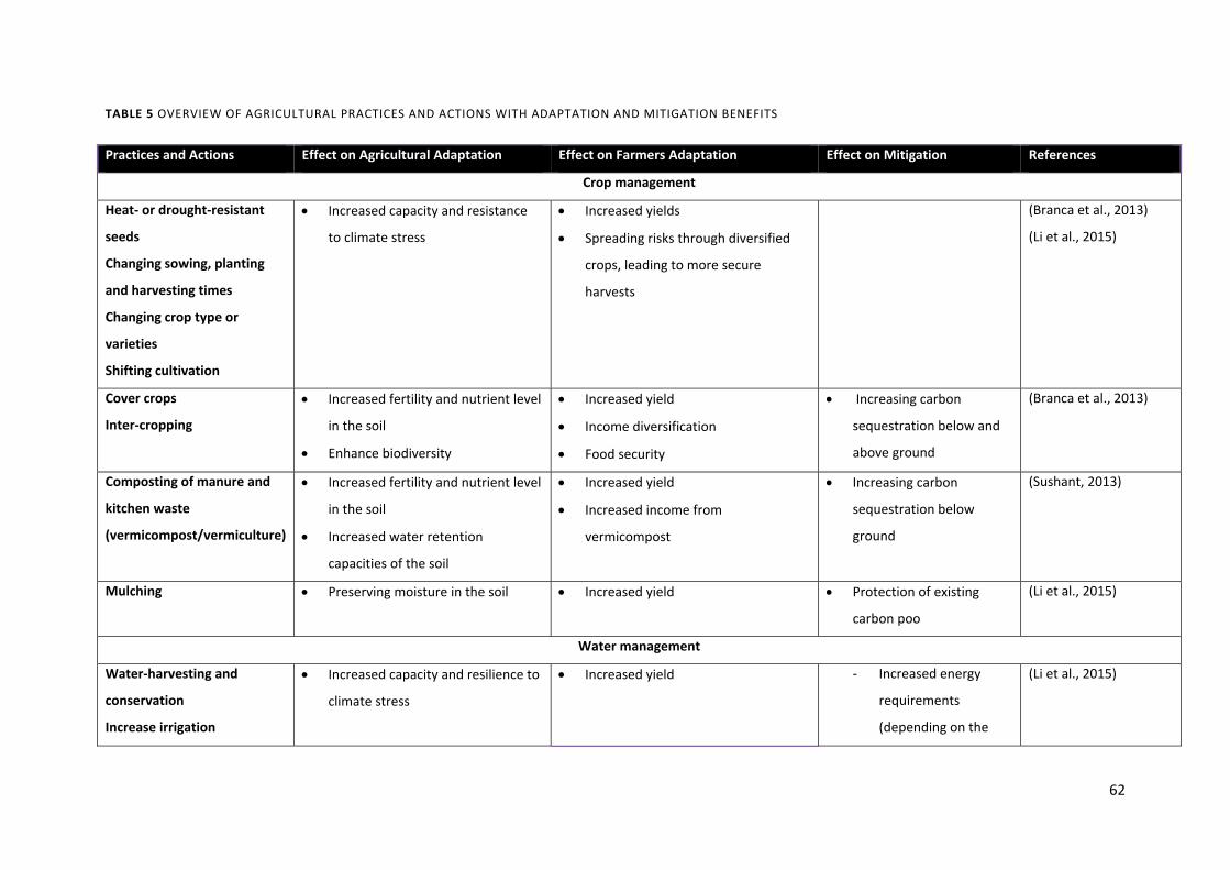
62  

TABLE 5 OVERVIEW OF AGRICULTURAL PRACTICES AND ACTIONS WITH ADAPTATION AND MITIGATION BENEFITS 

Practices and Actions Effect on Agricultural Adaptation Effect on Farmers Adaptation Effect on Mitigation References 

Crop management 

Heat‐ or drought‐resistant  

seeds 

Changing sowing, planting 

and harvesting times  

Changing crop type or 

varieties 

Shifting cultivation 

Increased capacity and resistance 

to climate stress 

Increased yields 

Spreading risks through diversified 

crops, leading to more secure 

harvests 

(Branca et al., 2013) 

(Li et al., 2015) 

Cover crops 

Inter‐cropping  

 

Increased fertility and nutrient level 

in the soil 

Enhance biodiversity 

Increased yield 

Income diversification 

Food security 

 Increasing carbon 

sequestration below and 

above ground 

(Branca et al., 2013) 

Composting of manure and 

kitchen waste 

(vermicompost/vermiculture) 

Increased fertility and nutrient level 

in the soil 

Increased water retention 

capacities of the soil 

Increased yield 

Increased income from 

vermicompost  

Increasing carbon 

sequestration below 

ground 

(Sushant, 2013) 

Mulching  Preserving moisture in the soil  Increased yield  Protection of existing 

carbon poo 

(Li et al., 2015) 

Water management 

Water‐harvesting and 

conservation 

Increase irrigation 

Increased capacity and resilience to 

climate stress 

 

Increased yield  ‐ Increased energy 

requirements 

(depending on the 

(Li et al., 2015) 

63  

Groundwater exploration for 

irrigation 

 

‐ unsustainable, if groundwater 

is a finite resource  

energy sources)

 

 

Landscape and land management

Management of organic soils 

Restoration of degraded land 

Better plant nutrient content  

Increased water retention 

capacities of the soil,  

Increased yield 

Greater adaptation capacity 

Protection of existing 

carbon pool 

(Campbell‐Lendrum et 

al., 2014) 

(Rosenzweig and 

Tubiello, 2007) 

Soil‐conservation techniques 

(organic fertilizer, reduced 

tillage and deep ploughing) 

Better plant nutrient content 

Increased water‐retention 

capacities of the soil 

‐ decreased yield in (short term) Increased carbon 

sequestration below 

ground 

 

(Branca et al., 2013) 

Diversification of the 

agricultural landscape  (e.g. 

crop diversification, 

agroforestry, tree cover, crop 

rotation) 

Including natural habitats 

and forest patches 

Risk reduction in relation to climate 

change impacts 

Enhance the availability of 

ecosystem services 

Resilience to pest and diseases 

among crops and livestock 

Enhance biodiversity  

Income diversification 

Food security 

 

Increase landscape carbon 

stock 

Increased carbon 

sequestration above and 

below ground 

Protection of existing 

carbon pool 

(C. A. Harvey et al., 

2014) 

(Branca et al., 2013) 

Planting of windbreaks and 

shade trees 

Protections of crops and livestock 

from climate stress 

Increased soil quality and fertility 

reduce Soil erosion and risk of 

landslides 

Income diversification 

Food security 

Protect people from climate stress 

 

Reduce carbon loss  

Increased carbon 

sequestration above and 

below ground 

Protection of existing 

(C. A. Harvey et al., 

2014) 

(Seck et al., 2005) 

(Jacobi et al., 2015) 

(Matocha et al., 2012) 

64  

Enhance biodiversity  carbon pool

Tree based home garden   protecting of smaller crops in the 

home garden from climate stress; 

sun, rain, wind etc. 

Enhanced biodiversity 

Income diversification  

Food security 

Protect people from climate stress 

Reduce hunger among children, 

because of the direct access to fruit  

Increased carbon 

sequestration above and 

below ground 

(Linger, 2014) 

Livestock

Silvo‐pastural system 

Rotation pasture 

The natural resources of the 

landscape are included as a 

measure of adaptation 

Enhanced biodiversity 

Climate‐tolerant legumes can be an 

alternative fodder source 

Food security 

Income diversification 

Reduction in cost of fertilizer for the 

fields, because of access to manure 

Protection of existing 

carbon pool 

Increasing carbon 

sequestration below 

ground 

Elimination of use of fire in 

pasture management  

(Jarvis et al., 2011) 

(Linger, 2014) 

(Steenwerth et al., 

2014) 

Converting livestock to more 

heat‐ or drought‐tolerant 

species 

Diversification of livestock  

Changing from crops to 

livestock  

Increased adaptive capacity to 

climate stress 

increased mobility 

Food security 

Income diversification 

Increased mobility for the household 

if they are forced to move 

Faster income reliefs in case of 

climate shocks  

 

Manure management to 

avoid emissions 

Mortality reduction of 

animals 

Reduction of deforestation 

and pasture burning 

through PES 

 

(Steenwerth et al., 

2014) 

(Li et al., 2015) 

 

Manure used for fertilizer  Increased fertility and nutrient level 

in the soil 

Increased crop yield 

Cost savings on fertilizer,  

Increased carbon 

sequestration below 

(Steenwerth et al., 

2014) 

65  

Increased water‐holding capacity,   ground

External support 

Farmers organisations Increased knowledge and 

knowledge sharing 

 

Social capital 

Increased capacity and resilience 

(Steenwerth et al., 

2014) 

Insurance of crops and 

livestock 

Create incentives for investment 

and income diversification 

‐ Risk of corruption among 

insurance verifiers 

Capital relief   Avoid exhausting soils 

Avoid deforestation and 

invasions of new land for 

agricultural areas 

protection of existing 

carbon pool 

(Jarvis et al., 2011) 

(Steenwerth et al., 

2014) 

Subsidies  Create incentives for investment 

and income diversification 

 

‐ Risk of corruption among 

program implementers 

Increased adaptive capacity and 

resilience  

Avoid exhausting soils 

Avoid deforestation and 

invasions of new land for 

agriculture  

protection of existing 

carbon pool 

(Steenwerth et al., 

2014) 

Extension services Increased knowledge and 

knowledge sharing 

Create incentives for new initiatives 

‐ Risk of corruption among staff 

implementing the extension 

services 

Increased adaptive capacity and 

resilience 

Increased awareness 

Avoid exhausting soils 

Avoid deforestation and 

invasions of new land for 

agriculture 

protection of existing 

carbon pool 

(Steenwerth et al., 

2014) 

PES or other income  Enhanced biodiversity  income diversification  Avoid exhausting of soils  (Steenwerth et al., 

66  

generating carbon schemes   

 

‐ Risk of corruption among 

program implementers 

Increased adaptive capacity and 

resilience 

Avoid deforestation and 

invasions of new land for 

agriculture 

 

2014)

3. JAM in Forestry  

 

Forests cover 31 per cent of the earth’s land surface (FAO, 2010), and climate change is likely to have 

a  wide  range  of  impacts  on  the  socio‐economic  systems  that  surround  forests  and  the  natural 

ecosystems of forests. In terms of biophysical  impacts, forests are  likely to experience range shifts, 

changes  in patterns of  tree  growth,  changes  in  insect  and disease  susceptibility  and distribution, 

changes in disturbance regimes such as fire, and changes in soil properties (Evans and Perschel, n.d.; 

Yuan  et  al.,  2011).  This will  reduce  the  capacity  of  natural  sinks  to  absorb  carbon  and  increase 

natural sources of CO2. Agriculture, Forestry and Other Land Use (AFOLU) activities have a feedback 

link  to  climate  change  in  that  these  activities  can  reduce  or  accelerate  climate  change,  affecting 

biophysical processes such as evapotranspiration and albedo (Yuan et al., 2011). Studies reviewed by 

the IPCC show that climate change may increase the frequency and severity of droughts in peatlands 

in particular and become a source of GHG (Yuan et al., 2011). 

In terms of socio‐economic impacts, shifts in natural ecosystems will influence how communities use 

and  depend  on  forests.  The  potential  for  forest  resources  to  contribute  to  rural  households  is 

becoming  increasingly apparent, as  studies of  the  contribution of  forest and wild products  to  the 

household income porfolio show that forest products on average represent 22 per cent of household 

incomes  (Angelsen  et  al.,  2014).  Indeed,  in  general  forests  can  fulfil  three  important  roles:  (1) 

support  current  consumption;  (2) provide  a  safety net  in  cases of  shocks  and  crises  and  fill  gaps 

during seasonal shortfalls; and (3) represent a means to accumulate assets and provide a path out of 

poverty (Angelsen et al., 2014). Furthermore, today the livelihood of millions of people, particularly 

the rural poor, are inextricably linked to forests (Angelsen and Wunder, 2003; Cammack, 2004). The 

consequences of shifting ranges and the distribution of forests and their products, as well as other 

disturbances, can thus leave the forest‐dependent poor particularly vulnerable.  

The  IPCC  has  calculated  that  forestry  and  other  land  uses  accounted  for  about  one  third  of 

anthropogenic CO2 emissions from 1750 to 2011 and for 12 per cent of emissions from 2000 to 2009, 

with a large proportion of that coming from changes to land use, mainly deforestation (Smith et al., 

2014).  Forest‐related mitigation  activities  are  therefore  a  relatively quick win  in  the  race  to  slow 

down the rate of carbon emissions. However, the socio‐economic and biophysical impacts of climate 

change  on  forests  and  vice  versa  significantly  affect  forests’  ability  to  function  as  a  carbon  sink. 

According to the latest Emissions Gap Report by the UNEP (2015), forest‐related mitigation activities, 

which  include  avoiding  deforestation  and  reducing  degradation,  afforestation  and  reforestation, 

 

68  

have  the  technical potential  to mitigate up  to 9 GtCO2 by 2030  if all  forest‐related activities  that 

degrade or clear the carbon sink were stopped today.  

Several characteristics specific to this sector can also have a bearing on the pursuit of JAM activities 

in this sector. First, the gestational period of forestry projects from idea to implementation tends to 

be quite long, and the benefits of mitigation cannot be harvested until many years later. This affects 

the permanence of  carbon  stocks, but  it  also makes  it more  susceptible  to  issues of  land‐tenure 

security,  particularly  since  forests  are  often  formally  owned  by  states,  but  managed  by  local 

communities (Ravindranath, 2007). As mentioned above, forests are also a source of food, shelter, 

medicine and  income, but  returns are often  low, and  forest‐based  livelihoods  rely heavily on  the 

subsistence use of resources   (Elias et al., 2014; Ravindranath, 2007). Hence, although challenging, 

achieving JAM in this sector is both socially and economically important.  

 

3.1   Forest‐Related Mitigation Activities that Lead to Adaptation Benefits 

Forests play a particularly  important role  in mitigation, mainly due to their capacity to sequestrate 

and store carbon. Deforestation and  forest degradation are believed  to have contributed 12.5 per 

cent  to global GHG emissions  from 1990  to 2010  through  tropical deforestation  (Houghton et al., 

2012).  The main mitigation  activities within  forestry  are  afforestation,  reforestation  and  avoiding 

deforestation  (IPCC,  2000).  Nevertheless,  mitigation  projects  have  the  potential  to  facilitate 

adaptation  by  reducing  pressure,  conserving  biodiversity  (through  conservation)  and  enhancing 

connectivity (Locatelli et al., 2011). 

Forestry mitigation projects, largely in the form of forest conservation, can facilitate the adaptation 

of  forests  to  climate  change  by  reducing  the  anthropogenic  pressure  on  forests,  enhancing  the 

connectivity between  forest  areas  and  conserving biodiversity hotspots  (Locatelli, 2011).  Forestry 

mitigation  projects  can  also  reduce  vulnerability  and  promote  adaptation  through  forest 

conservation, protected area management and  sustainable  forest management, but  they  can also 

have consequences for adaptive responses and/or the development objectives of other sectors (for 

example,  expansion  of  farm  land)  (Smith  et  al.,  2014).  Importantly,  forestry mitigation  activities, 

including  conservation  actions,  are  relatively  more  cost‐effective,  safe  and  easy  than  other 

mitigation  actions  (in  other  sectors)  and  are  therefore  seen  as  a  critical  strategy  in  reducing 

emissions (Nabuurs et al., 2007; Ravindranath, 2007; Turner et al., 2009). Given the limited need to 

rely on  technological development,  it has been argued  that ecosystem  restoration will  remain  the 

only realistic large‐scale climate change mitigation mechanism for the coming decades (Turner et al., 

2009). However, strict conservation alone can also have negative effects, such as restricting access 

 

69  

to  land  and  forest  resources,  as well  as  encouraging  dependence  on  external  funding  (Locatelli, 

2011).  The  resilience  of  a  natural  diversified  forest  ecosystem  is  much  greater  than  that  of  a 

monoculture  plantation,  as  the  former  is more  resilient  to  disturbances  and  provides  important 

ecosystem services, such as water and microclimate regulation (Turner et al., 2009). 

Plantation  establishment  through  afforestation  or  reforestation  can  also  be  an  effective way  of 

sequestering carbon and preventing other environmental disasters, such as desertification, just as it 

can represent a useful source of income. The Carbon Farming Initiative, developed by the Australian 

government,  is a voluntary  carbon offset  scheme  rewarding  farmers and  landholders  through  the 

carbon credits system for actions to store carbon on their land (afforestation or reforestation) or to 

reduce  GHG  emissions  (Commonwealth  of  Australia,  2013).  However,  other  concerns  related  to 

plantation  establishment,  such  as  preserving  biodiversity,  are  only  incorporated  as  safeguarding 

measures  (van Oosterzee, 2012).  Indeed,  ,  if plantations  reduce biological diversity,  they may also 

reduce  the  capacity of people  to  adapt  to  climate  change.  Furthermore, monocultures  are often 

more vulnerable to climate change than other cultures (Campbell‐Lendrum et al., 2014). 

 

3.2   Forest‐Related Adaptation Activities that Lead to Mitigation Benefits 

Forests  play  an  important  role  in  adaptation.  ‘Adaptation  for  forests’  refers  to  the  adaptation 

needed for forests to maintain their function (Locatelli et al., 2011). Such adaptation strategies for 

forests can include the anticipatory planting of species along latitudes and altitudes, assisted natural 

regeneration,  mixed‐species  forestry,  species‐mix  adapted  to  different  temperature  tolerance 

regimes, fire protection and management practices, thinning, sanitation and the  intensive removal 

of  invasive  species,  surplus  seed  banking,  altering  harvesting  schedules  and  other  silvicultural 

practices. Moreover, it can include the in‐situ and ex‐situ conservation of genetic diversity, drought 

and  pest  resistance  in  commercial  tree  species,  the  adoption  of  sustainable  forest management 

practices, increasing protected areas and linking them, when possible, to promote the migration of 

species,  forest  conservation  and  reduced  forest  fragmentation  enabling  species  migration,  and 

finally  energy‐efficient  fuelwood  cooking devices  to  reduce  the pressure on  forests  (Millar  et  al., 

2007)).  

 

70  

Box 6. Ecosystem‐based adaptation (EbA)  

EbA projects are characterised by integrating the use of biodiversity and ecosystem services into an 

overall strategy  to help people adapt  to  the adverse  impacts of climate change, can contribute  to 

mitigation  by  increasing  or maintaining  carbon  stocks  in  forests  (Colls  et  al.,  2009).  Though  EbA 

encompasses many different types of ecosystems, forests play a central role as they are often major 

providers of ecosystem services (Locatelli et al., 2010). The costs of maintaining ecosystems may be 

lower and the end results can be more effective than for more sophisticated adaptation measures. 

Although  clearly  a  human‐oriented  adaptation  strategy,  there  are  clear  mitigation  benefits  of 

conserving forests and avoiding emissions. Within EbA, mitigation approaches such as REDD+ or PES 

can also be utilised to ensure that project objectives also focus on mitigation (Rizvi et al., 2015).  

EbA  can also be used  to ensure  the provision of particular ecosystem  services  that are  crucial  for 

human  adaptation,  for example water  regulation  (Locatelli et  al., 2010).  For example,  sustainable 

watershed management  is recognised as crucial  in stabilising water supplies to African cities, which 

will face water scarcity in the future (Mafuta et al., 2011). At the same time, conservation of forested 

areas  ensures  the  preservation  of  carbon  stocks.  Further  examples  of  EbA  can  be  found  in  the 

tsunami‐affected areas of South and Southeast Asia, where coastal ecosystems were  rehabilitated 

with mangroves  and  other  coastal  vegetation,  increasing  the  carbon  storage  potential  (Wetlands 

International Report, 2011). Mangroves also dissipate wave energy, rendering the  impact of storms 

and other climatic events  less severe  for both people and the coastline. Another example  is  forest 

fire management in West Arnhem Land in Northern Australia. Mitigation benefits include limiting or 

preventing wildfire  emissions, but  the  initiative  also  increases  the  adaptive  capacity of  forests  to 

extreme climatic events, which may lead to increased fire frequency and intensity (ProAct, 2008). 

Strengthening the resilience of forests also increases the permanence of carbon (Malhi et al., 2009).  

’Forests for adaptation’ refers to how forests can support households in their adaptation to climate 

change and in coping with climatic change by acting as safety nets, gap‐fillers and providers of local 

environmental  services  in  response  to  climate‐related  fluctuations  with  lower  food  availability 

(Locatelli et al., 2011). Ecosystem‐based adaptation is one example of this (see Box 6). Pramova et al. 

(2012) provide  an overview of  five  cases where  forests  and  trees  contribute  to  adaptation.  First, 

forests and trees can represent goods to local communities facing climate impacts. Second, trees on 

farms can regulate the soil, water and microclimate, thus facilitating more climate‐resilient forms of 

production. Third,  forested watersheds  regulate  the water and protect  the soil. Fourth, mangrove 

forests  can protect  coastal areas.  Fifth, urban  forests  can  regulate  the  temperature and water of 

 

71  

cities. Rural households  are destined  to be  among  those  that  are most  affected by  the  changing 

climate,  including  impacts  such  as  decreased  rainfall  and  increased  storms  and  damage  that 

threaten  resource‐based  livelihoods,  including  agriculture.  With  intensified  impacts  of  climate 

variability in other sectors such as agriculture, water and energy, forests may come to play an even 

more important role as safety nets (Angelsen et al., 2014; Nkem et al., 2010). For example, ‘trees on 

farm’ systems are used to provide shade, reduce temperatures and lessen the impact of hard rainfall 

and  wind,  both  for  certain  crops  (agroforestry  systems)  and  livestock  (silvipastoral  practices) 

(Verchot  et  al.,  2007).  Conversely,  climate  shocks  can  enhance  people’s  harvesting  of  forest 

products,  thereby degrading  the  forest base, particularly  if climate  shocks become more  frequent 

and  intense    (Locatelli,  2011).  Adaptation  and  forestry  mitigation  projects  can  be  linked  by 

incorporating  standards  for  adaptation  into  forest  carbon  certification  and  strengthening  the 

capacities of project developers to accommodate both components (Kongsager and Corbera, 2015). 

National and  international policies can also create conditions to facilitate the development of JAM 

activities (Locatelli, 2011). 

 

3.3   Integrated and Synergetic Activities 

Activities  contributing  to  conservation  and  reduced  deforestation  can  have  mitigation  benefits 

through  carbon  sequestration  and  carbon  storage,  as well  as  a  range of  adaptation benefits.  For 

example,  reduced  deforestation  can  be  achieved  by  reducing  the  dependence  on  land‐based 

economic  sectors  (for  example,  agriculture  and  livestock)  and  by  creating  environments  that 

facilitate  such development  (for example,  removing  the  subsidies  that encourage aggressive  land‐

clearing). REDD+ aims  to  reduce carbon emissions  from deforestation and  forest degradation and 

covers both sustainable forest management and the enhancement of carbon stocks. It has become 

an important policy tool that will allow forest‐rich countries to offset their carbon emissions. REDD+ 

has gained increasing traction, but it was only in the recently signed Paris Agreement (2015) that it 

was    recognised  as  a  viable  path  to  reductions  in  CO2  emissions.  Though  REDD+ was  originally 

envisioned as an international PES scheme (see Box 1 for example,  Angelsen et al., (2009), it is now 

apparent that emerging REDD+  initiatives are continuing  integrated conservation and development 

strategies  (Sunderlin  et  al.,  2014a).  Indeed,  less  than  half  of  the  23  incipient  REDD+  projects 

reviewed by Sills et al. (2014) were making conditional payments for actions to reduce deforestation 

and degradation. Nevertheless, adaptation benefits from such payment programmes can contribute 

to  enhancing  households’  economic  resilience,  while  also  achieving mitigation  benefits  through 

preserving  carbon  stocks.  In  the  cases  reviewed  by  (Caplow  et  al.,  2011),  positive  income  and 

 

72  

employment benefits were found; particularly in the Noel Kempff Mercado Climate Action Project in 

Bolivia, mitigation  activities  have  produced  positive  livelihood  impacts  through  the  promotion  of 

livelihood  activities  supporting  conservation  and  sustainable  management.  The  same  project, 

however, suffered from poor inclusion and project coordination, largely due to the scale of the area 

involved,  similar  to  the  issues  that  concern  conservation  and    development  projects  (May  et  al., 

2004).  Another  example  is  the  Bolsa  Floresta  programme  (also  known  as  the  Forest  Allowance 

programme) in the Amazon, which emphasises sustainable livelihood development, while achieving 

mitigation benefits through forest conservation (Börner et al., 2013). 

Expanding or establishing protected areas  can also  lead  to mitigation and adaptation benefits  for 

forests,  biodiversity  and  people.  For  instance,  conservation  corridors  enable  wildlife  to migrate 

between areas  for  food and  shelter.  Intact  forests  lead  to  increased ecosystem  resilience and  the 

provision of  regulating environmental  services,  such as water‐cycling and microclimate  regulation. 

Finally, greater ecosystem  resilience achieved  through conservation can  conserve biodiversity and 

reduce susceptibility to disturbances such as fire. People also benefit from such activities by being 

less affected by disturbances, having access  to a  resource base and  regulating ecosystem  services 

that can help them adapt to climate change. Indeed, conservation actions are  increasingly relevant 

to  forest‐dwelling communities, which may  rely on  forest products  to diversify  income  streams  in 

times of need or on forests for current consumption. Another coping strategy is harvesting of forest 

products (Fisher et al., 2010), which may serve an important function in the face of the increasingly 

unstable  climate  and  its  impact  on  food  supply.  Enhanced  soil  fertility  and  soil  protection  can 

increase the productivity of small‐scale agriculture, which may in turn lead to reduced land‐clearing. 

Nevertheless,  overharvesting  and  forest  degradation  can  become  problematic  if  the  severity  and 

frequency  of  climate  shocks  increase  (Locatelli  et  al.,  2011).  On  the  other  hand,  designating 

protected  areas  and  placing  restrictions  on  forest  use may  limit  the  consumption  of  forests  and 

forest products, as well as restrict access to resources that people may depend on (Streck, 2009). 

Activities aimed at reducing degradation may focus on sustainable forest management activities or 

practices that reduce the risk of disturbances such as fires or pests. Sustainable forest management, 

defined as  ‘a dynamic and evolving concept aiming  to maintain and enhance  the economic, social 

and environmental values of all types of forests for the benefit of present and future generations’ 

(UN, 2008), represents a holistic approach to forest management. The failure to manage forests in a 

sustainable way drastically reduces their adaptive capacity; this includes benefits such as increasing 

ecosystem resilience to climate change, soil erosion protection, soil fertility enhancement and even 

watershed  and microclimate  regulation,  depending  on  the  degree  of  restoration  (Locatelli  et  al., 

 

73  

2010). Clearly, a reduction  in forest disturbances will positively benefit people’s ability to adapt to 

climate  change  and  reduce  the  impact  of  that  on  household  economy  and  productivity.  Fire 

management practices  can have  important adaptation benefits, especially  in  the hotter and drier 

climates  of  fire‐prone  areas,  as  well  as  mitigation  benefits,  as  carbon  stocks  are  preserved  or 

maintained  (Matocha et  al., 2012). However,  some adaptive measures,  such as  reducing  rotation 

times or suppressing fires, can jeopardise the permanence or decrease carbon stocks in the long run. 

Sustainable forest management can also be implemented with mitigation as the main objective, for 

instance,  in  fire management. While  fires  are  necessary  for  some  ecosystems  to maintain  their 

function,  in  others  the  results  can  be  devastating,  leading  to  slow  regrowth,  lost  biomass  and 

reduced ecosystem services (Elias et al., 2014). More frequent and  intense fires can make systems 

such as the Amazon rainforest reach a tipping point beyond which the forest cannot bounce back, 

resulting in a transition to grassy savannah‐type environments (Nepstad et al., 2008). 

 

Activities associated with afforestation and reforestation can lead to the direct mitigation benefits of 

restoring carbon stocks. Adaptation benefits for people  include the provision of wood fuel to meet 

current  resource  demands  and  thereby  reduce  pressure  on  other  natural  forest  areas. 

Environmental services such as water regulation,  flood and erosion control can result  in  improved 

water availability and water regulation, soil conservation and increased arable land (Somorin et al., 

2012). This  is particularly  true of water‐abundant  regions or areas  that experience  intense  rainfall 

seasons  interspersed with  long dry spells  (Locatelli et al., 2011). Such soil and water conservation 

benefits can reduce the impacts on tree growth. For forests, short‐rotation species in commercial or 

industrial  forestry  or  silvicultural  practices,  for  example,  sanitation  harvests,  can  reduce 

susceptibility to pests and disease. However, afforestation and reforestation activities have certain 

negative effects. In semi‐arid and arid regions, the demand for water can be high and will increase in 

hotter climates, while  forestry is more water‐demanding than other land uses (FAO, 2008; Klein et 

al.,  2007a).  Other  concerns  are  land  use  and  availability.  For  instance,  reforestation  plans may 

conflict with  future demands  for  land  for  cultivation  in  the  face of  climate  changes and,  thereby, 

land  productivity  (arable  land).  Biodiversity  can  also  be  affected  through  monocultures  in 

afforestation  and  reforestation, which  promote  fast‐growing  alien  species  (Klein  et  al.,  2007).  To 

minimise  trade‐offs,  afforestation  and  reforestation  activities  can  ensure  the  use  of  diverse  tree 

species or native  tree species  (Ravindranath, 2007) or planting  in degraded or marginalised  lands, 

thus enhancing sustainable forest management (Duguma et al., 2014). 

Overall several synergetic or integrated activities can be achieved within forestry, leading to greater 

cost and project efficiency (Somorin et al., 2012). An overview of integrated and synergetic practices 

 

74  

and actions in forestry that result in mitigation and adaptation benefits is given in Table 3. The three 

columns  note  the  positive  and  negative  effects  of  these  practices  and  actions  on  1)  forest 

adaptation, that is, how practice contributes to or detracts from building forest resilience to climate 

change impacts; 2) people's adaptation, that is, how practice contributes to or detracts from building 

people's  resilience  to  climate  change  impacts,  particularly  forest‐dependent  people;  and  3) 

mitigation.

 

75  

TABLE 6 OVERVIEW OF PRACTICES AND ACTIONS IN FORESTRY WITH ADAPTATION AND MITIGATION BENEFITS 

Practices and Actions Effect on Forest Adaptation Effect on People's Adaptation  Effect on Mitigation Reference

Conservation and reduced deforestation

Avoided/reduced 

deforestation of forests, e.g. 

changes in policies, 

economic growth sectors 

Increase in ecosystem resilience 

to climate changes 

Soil erosion protection and soil 

fertility enhancement 

Watershed regulation 

Microclimate regulation 

Microclimatic regulation for 

people, livestock, crops and 

wildlife 

Coastal area protection 

Increase in crop resilience 

Increase and enhance carbon 

sequestration above and 

below ground   

 

Protecting against watersheds 

can benefit hydropower and 

clear energy 

(Locatelli et al., 2015) 

(Malhi et al., 2009) 

 

Avoided deforestation 

through REDD+/payments 

for environmental services 

Payments can contribute to 

household welfare, improve 

economic resilience 

 

(Campbell, 2009) 

(Jarvis et al., 2011) 

Expansion or formation of 

protected areas 

Linking areas through corridors  

Reduced impact logging 

Conserving biodiversity  

Reducing disturbances, e.g. fire 

Preserving resource base as 

household safety net 

Preserving ecosystem services, 

e.g. water regulation 

Diversify livelihoods and incomes 

‐ Competition for land/ 

decreased access to land 

‐ overuse of forest resources 

for coping with climate shock, 

can lead to degradation of the 

forest  

(Brown et al., 2011) 

(Mustalahti et al., 2012) 

(Alexander et al., 2011) 

 

 

(Locatelli et al., 2011) 

(Athanas and 

McCormick, 2013) 

(Stromberg et al., 2011) 

 

 

76  

Reduced degradation 

Fire management and 

protection 

‐ Shortened rotation times to adapt 

to CC can decrease carbon stocks 

‐ Fire suppression can jeopardise 

permanence of carbon stocks 

Early warning and improved fire 

fighting 

Microclimatic regulation for 

people and crops 

Increase in crop resilience 

Preserving resource base as 

household safety net 

Preserving ecosystem services, 

e.g. water regulation 

Diversify/uphold livelihoods and 

incomes 

‐ Decrease in carbon 

stocks 

‐ Permanence of carbon 

stocks 

 

Reduced/limited GHG 

emission as a result of 

reduced intensity 

(Couture and Reynaud, 

2009) 

(ProAct, 2008) 

(Swart and Raes, 2007) 

Sustainable forest 

management, including 

pest/disease management 

Restoring degraded natural 

forest land through regeneration 

of native species and natural 

regeneration of degraded land 

Increase in ecosystem resilience 

to climate change 

Reduce disturbances, e.g. 

through fire‐protection regimes 

Soil‐erosion protection and soil‐

fertility enhancement 

Watershed regulation  

Microclimate regulation 

Increase and enhance carbon 

sequestration, and carbon storage 

above and below ground 

 

(Ravindranath, 2007) 

(Duguma et al., 2014) 

Sequestration

Afforestation 

 

Reduce susceptibility to 

pest/disease through e.g. short 

Meeting current resource 

demands, e.g. wood fuel 

Increase and enhance  (Ravindranath, 2007) 

(Duguma et al., 2014) 

 

77  

 

 

 

 

 

 

 

 

rotation species in commercial 

or industrial forestry or 

silvicultural practices, e.g. 

sanitation harvests  

Reduce adverse impacts on tree 

growth through e.g. soil and 

water conservation measures 

 

‐ Reduced ecological adaptation 

(fast‐growing monocultures are 

more vulnerable) 

 

Regulation of environmental 

services, e.g. water 

Stabilise slopes and reduce 

flooding 

Lower vulnerability to heat stress 

carbon sequestration, and 

carbon storage above and 

below ground 

‐ Some trees may not be as 

effective in sequestering 

carbon 

(Dang et al., 2003) 

(Klein et al., 2007a) 

Reforestation ‐ Decreased food security 

‐ Compete for land 

‐ Short‐term benefits for few 

‐ Reduction in water availability in arid 

regions  

‐ Reduced ecosystem resilience 

resulting from monocultures 

 

 

 

 

 

 

 

(Stringer et al., 2012) 

(Beymer‐Farris and 

Bassett, 2012) 

(Schrobback et al., 

2009) 

(D’Amato et al., 2011) 

 

 

78  

4. Barriers and Opportunities to Joint Activities in Agriculture and Forestry 

 

4.1   Institutional and Policy Barriers and Opportunities

Institutional and policy barriers and opportunities can both hinder and facilitate the development of 

JAM  activities.  At  the  national  level,  Locatelli  et  al.  (2011)  found  that  in  Latin  America  national 

policies are rarely set up to accommodate the integration of adaptation and mitigation activities, the 

strongest focus still being on mitigation activities. They also found that in CDM projects in Colombia 

the government recognised  the  lack of an adaptation requirement  in  the approval process. At  the 

national  level,  adaptation  and  mitigation  were  managed  by  separate  ministries  or  institutions, 

largely due to differences in sectoral focus and geographical scales of implementation. Policies that 

are uncoordinated and, at times, conflict  in the areas of climate change mitigation and adaptation, 

food security and economic development can generate perverse incentives that can unintentionally 

lead to the unsustainable use and overuse of resources  and conflicting goals, hindering a more all‐

inclusive  approach  to  joint  activities  (Campbell  et  al.,  2011;  Hoffmann,  2011).  For  example,  the 

fragmentation  of  mandates  and  tasks  by  different  government  agencies  is  one  of  the  main 

challenges in moving REDD+ projects ahead in Vietnam and Indonesia (Thuy et al., 2014). 

At the international level, the story is similar to the country‐specific one above. The UNFCCC treats 

mitigation and adaptation as separate policy measures (Duguma et al., 2014), though recognition of 

joint adaptation and mitigation measures has been growing.  International agreements have had a 

strong focus on mitigation, for example, setting emissions targets under Kyoto (Locatelli et al., 2010), 

while adaptation is viewed as a means to achieve mitigation (Duguma et al., 2014). Adaptation and 

mitigation  are  addressed  through  different  processes  and  are  discussed  in  corresponding  policy 

debates  that  are  rarely  linked  and  that  can  involve  different  constituencies  and  funding  sources 

(Harvey et al., 2014; Verchot et al., 2007).  

Reasons  for  this  may  be  because  in  many  cases  policy  planning  is  short  term,  whereas  the 

integration  of  adaptation  and  mitigation  goals  requires  long‐term  planning  as  a  result  of  their 

varying time scales for implementation and effect (Harvey et al., 2014). For instance, in some cases 

policies supporting conventional agricultural practices predominate over those supporting climate‐

smart  agriculture. However, promoting multi‐stakeholder  planning  across  local,  regional,  national 

and business interests could avoid this barrier by raising awareness among policy‐makers and other 

decision‐makers about activities with adaptation and mitigation goals – for  instance, (i) developing 

NAPAs,  NAMAS  and  REDD+  strategies  that  include  JAM  practices,  or  (ii)  securing  high‐level 

commitments to conservation agriculture, agroforestry and other climate‐smart agriculture practices 

 

79  

(Harvey  et  al.,  2014),  as  well  as  incorporating  JAM  objectives  directly  into  sector  policies  (e.g. 

forestry  (Locatelli et al. 2015).  

 

4.2   Knowledge and Capacity Barriers and Opportunities  

The fundamental divide between mitigation and adaptation also affects the way project developers 

think of their projects, as is evident from the large number of projects that can potentially contribute 

win‐win outcomes for both adaptation and mitigation, but fail to do so (Locatelli et al., 2011). 

Empirical studies of the synergies in forestry and agriculture are few, and more research is needed to 

explore  these  linkages  in  forests at  the  levels of  landscapes, projects,  countries and  international 

agreements  (Naidoo et al., 2008). Methods  for assessing the magnitude of  the ecosystem services 

that are generated  through  forest conservation and  reforestation are needed, as are methods  for 

measuring  the  role of ecosystem  services  in  reducing  the vulnerability of  communities  to  climate 

change  (Locatelli et al., 2011; Naidoo et al., 2008). The difficulty associated with documenting and 

collecting data on the benefits of ecosystem services amongst users often plays a central role (FAO, 

2015) (FAO, 2015). 

Moreover, at the individual level, farmers may face another  level of   barriers, namely tradition and 

the  social  acceptability  of  change,  which  can  ultimately  affect  their  willingness  to  adopt  new 

initiatives. This results in the need for awareness and communication of the need for and benefits of 

climate  change  adaptation  initiatives  (Smith  and Olesen,  2010).  Related  to  this, capacity  barriers 

have  become  increasingly  relevant.  The  failure  of  extension  services  in  some  African  countries 

restricts the ability to upscale  innovations  in agroforestry for  improved  land‐use systems (Mbow et 

al.,  2014).  Specifically,  knowledge  of  advanced  cultivation  methods  and  technical  support  is 

necessary before farmers can add trees to cropping systems and/or animal production, and  it may 

also promote the swift adoption of agroforestry techniques (Matocha et al., 2012).   

There  is  a  technical  difference  between  mitigation  and  adaptation  concerning  their  physical 

evaluation, where single‐metric GHG emissions exist for mitigation, but not for adaptation (Watkiss 

et al., 2015). Moreover, there are no metrics for evaluating the synergetic benefits of mitigation and 

adaptation (Duguma et al., 2014). The synergetic effects have only recently begun to be described, 

and there is still some scientific uncertainty as to what constitutes the optimal mix of adaptation and 

mitigation, when the goal is to achieve the best benefits of different kinds of synergies (Klein et al., 

2005). Moreover,  both  adaptation  and mitigation  suffer  from  other methodological  challenges: 

there are high levels of uncertainty and large costs involved in measuring and monitoring emissions 

 

80  

reductions,  including  complications  in  establishing  a  baseline.  REDD+  projects  in  particular  face 

significant  methodological  challenges  with  regard  to  linking  co‐benefits  to  carbon  benefits,  as 

common measures  for  evaluating  biophysical  and  welfare  outcomes  still  need  to  be  developed 

(Caplow  et  al.,  2011). At  the  landscape  level  it  is  essential  to  track  and monitor  the  diversity  of 

farming    and  the  changing  impacts  and  threats  facing  farming  (e.g.  of  agricultural  production, 

ecosystem services and human welfare) in order to monitor the synergies and trade‐offs of different 

agricultural development scenarios and inform future sustainable agricultural development (Sachs et 

al., 2010). 

To solve the existing technical, knowledge and capacity‐building barriers, Harvey et al. (2014) have 

argued that it is necessary to develop tools for policy‐makers and other decision‐makers to visualise 

the  potential  outcomes  of  different  joint  strategies  concerning mitigation  and  adaptation,  food 

production, energy,  incomes and other related objectives. More analytical assessments of ongoing 

JAM  initiatives  and  projects  can  therefore  provide  the  evidence  for  when  and  where  pursuing 

adaptation and mitigation  simultaneously  is more beneficial and cost‐effective  than  implementing 

them  separately. Also  knowing  the  impact  of  future  climate  change  on  current  joint  activities  is 

essential,  for  example,  knowing  how  tree  species  distributions  will  change  in  future  climate 

scenarios, particularly if agroforestry relies on a certain tree species. Importantly, there is a large gap 

in our knowledge of how mitigation can benefit from adaptation (and vice versa) and of the added 

value of  integrated  strategies. Also,  certain  contextual  factors  should be  in place  that  can  largely 

determine whether mitigation and adaptation should be pursued separately or combined, but this 

knowledge also needs to be acquired (Locatelli et al., 2015). 

 

4.3   Funding and Other Barriers and Opportunities 

Funding  bodies  often  look  at  mitigation  and  adaptation  separately,  and  current  funding  of 

adaptation  and  mitigation  projects  rarely  takes  synergies  into  account  (Duguma  et  al.,  2014; 

Kongsager et al., 2015). In addition, many mitigation and adaptation projects have been on a small 

to medium scale; hence,  identifying  the project‐level capacity of  JAM can perhaps be achieved by 

first  identifying the adaptation co‐benefits of mitigation projects or vice versa (Illman et al., 2012). 

Project  standards  such  as  the Voluntary Carbon  Standard only  consider  the  livelihood  impacts of 

mitigation activities, not of adaptation. However, a concept  like PES and payment schemes such as 

REDD+  and  co‐investment  schemes  (Namirembe  et  al.,  2014)  show  increasing  potential when  it 

comes  to  incorporating  adaptation  activities.  The Climate Gold  Level of  the CCB  Standards’ Third 

Edition  adopts  an  optional  criterion,  which  can  be  used  to  identify  and  promote  projects  that 

 

81  

provide  significant  support  to  communities  and/or  biodiversity  with  regard  to  adapting  to 

anticipated climate change impacts and risks (Namirembe et al., 2014). This is a starting point for the 

joint funding of JAM activities. 

Even though there are indications that certain climate management practices generate savings over 

their  lifecycle, many also  involve upfront  costs and  short‐term  risks  (FAO, 2009; Hoffmann, 2011; 

McKinsey, 2009). For example, soil and water conservation infrastructures can require large upfront 

costs in terms of labour and external efforts (FAO, 2009). Although the financial incentives for some 

mitigation  practices  may  take  the  form  of  agricultural  carbon  credits,  and  some  only  benefit 

smallholders, a number of  issues need to be taken  into consideration here to enhance the options 

for carbon  incomes to create  incentives for adaptation  initiatives and thus overcome the barrier of 

underfunded adaptation initiatives. 

The lack of joint coordinated funding streams for adaptation and mitigation is another key constraint 

(Buchner et al., 2013; FAO, 2013). The private sector and carbon finance represent the main sources 

of funding for mitigation activities, whereas public funds, NGOs and donors often prioritize poverty 

alleviation, food security or disaster relief, which tends to complement adaptation priorities (Lobell 

et  al.,  2013;  Schalatek  et  al.,  2012).  This  traditional  separation  of  funding  sources  (and  funding 

eligibility criteria) has created silos in the implementation of adaptation and mitigation measures on 

the ground (Schalatek et al., 2012), as well as hindering the adoption of  integrated  landscape‐level 

approaches (Harvey et al., 2013; FAO, 2013). 

In REDD+ projects, tenure security poses a major barrier  (Kongsager and Corbera, 2015; Sunderlin et 

al.,  2014a). Without  secure  tenure  and  rights  to  use  forest  resources,  the  potential of  forests  to 

support local communities and our chances of further developing REDD+ will be limited (Sunderlin et 

al., 2014a). Recent evidence has shown that transfers of ownership of large areas of forest commons 

to  communities  coupled with  carbon  payments  can  both  contribute  to mitigation  and  introduce 

livelihood  improvements  (Chhatre  and Agrawal,  2009). Moreover,  the  twenty  to  thirty‐year  time 

scale of REDD+ projects creates uncertainty when it comes to evaluating whether such projects will 

indeed have positive outcomes (Caplow et al., 2011). 

   

 

82  

 

5. Conclusion 

 

The present  review of  the concepts and practices of  joint adaptation and mitigation  in agriculture 

and forestry highlights the complexity and challenges involved in both defining and operationalising 

joint activities.  Issues such as the differences between adaptation and mitigation activities in terms 

of scale of  implementation,  time horizon  for  implementation, availability of  funding  for mitigation 

versus  adaptation  and  the  metrics  to  measure  mitigation  versus  adaptation  pose  significant 

challenges to the pursuit of joint activities.  

Land use is one of the key sectors that has great potential for creating synergies between mitigation 

and adaptation actions, potentially achieving both objectives at  little or no extra cost.  Importantly, 

mitigation  and  adaptation  in  two  of  the  major  land  uses  –  agriculture  and  forestry  –  have 

interconnected  effects on  agriculture or  forest  ecosystems  and on  society, making  the pursuit of 

joint  activities  even more  complex,  but  at  the  same  time  offering mutual  benefits.  The  positive 

benefits  of  adaptation  can  also  be  mutually  beneficial  for  development,  and  often  positive 

development  benefits  are  likely  to  contribute  to  positive  effects  on  people's  adaptive  capacity. 

Moreover, the positive nature of these benefits, showcased by empirical studies  in Tables 2 and 3, 

emphasises the need to pursue  joint activities and further research to understand the barriers and 

opportunities to operationalisation. 

The current coverage of joint adaptation and mitigation in the literature has also been piecemeal, as 

there is no one definition of a joint adaptation‐mitigation activity. At best, scholars have attempted 

to describe  the  linkages,  interrelationships, complementarity, substitutability, synergies and  trade‐

offs that currently exist  in empirical examples  in agriculture and forestry, among others. From this 

we  have  compiled  the  major  activities  that  can  be  categorised  into  mitigation  activities  with 

adaptation benefits, adaptation activities with mitigation benefits, integrated or synergetic activities, 

and importantly their effects on agriculture or the forest ecosystem and on society.  

The paper has also highlighted existing barriers and opportunities within agriculture and forestry in 

pursuing JAM – this is the first step in highlighting the specific areas that suffer from policy, financial, 

knowledge  and  capacity  barriers  and  opportunities  that  hinder  or  facilitate  the  pursuit  of  JAM 

activities.  This  also  provides  insights  into  where  efforts  can  be  focussed  to  ensure  the  further 

development  of  JAM  activities  and  the  tools  necessary  for  succeeding.  Examples  include making 

funding available for joint adaptation and mitigation activities, encouraging collaboration in order to 

 

83  

challenge  the  current  policy  division  between mitigation  and  adaptation,  and  promoting  further 

documented  research measuring  the  impacts  of  joint  activities,  their  cost‐effectiveness  and  their 

synergies within the complex setting of risks and uncertainty concerning the magnitude of climate 

change impacts. 

Moving forward, in the pursuit of joint adaptation and mitigation activities, it is important to keep in 

mind  the  objectives  of  pursuing  JAM  activities  simultaneously  in  order  to  provide  cost‐effective, 

sustainable solutions that capitalise on the mitigation and adaptation effects of a particular activity 

to the mutual benefit of both. Simply striving for win‐win outcomes for the sake of doing so may put 

at risk other activities which may achieve important adaptation‐ or mitigation‐only benefits, thereby 

diminishing the effective use of limited climate funding (Klein et al., 2005). 

Indeed,  identifying an optimal mix of adaptation and mitigation  is a slow and tedious process, one 

that is likely to vary between countries and over time (Klein et al., 2015). Thus, country‐specific and 

context‐adapted  responses are vital  to  the design of  JAM activities and  their eventual  success.  In 

particular,  the enabling conditions  that can  facilitate  the pursuit of  joint activities also need  to be 

understood, enhanced and/or established in order to support the full pursuit of joint activities where 

relevant and thus complement the fulfilment of national ambitions highlighted in the INDCs, as well 

as  in  global  targets  such  as  the  Sustainable  Development  Goals  and  the  Paris  Agreement,  thus 

ultimately setting the world on track to a low‐carbon and climate‐resilient future.  

 

6. Acknowledgements 

 

We would like to thank Rico Kongsager, Lars Christiansen, Anne Olhoff and Jette Bredahl Jacobsen 

for review comments. 

 

7. References 

  

Abid, M., Scheffran, J., Schneider, U.A., Ashfaq, M., 2015. Farmers’ perceptions of and adaptation strategies to climate change and their determinants: the case of Punjab Province, Pakistan. Earth Syst. Dyn. 6, 225–243. doi:10.5194/esd‐6‐225‐2015 

Alexander, S., Nelson, C.R., Aronson, J., Lamb, D., Cliquet, A., Erwin, K.L., Finlayson, C.M., De Groot, R.S., Harris, J.A., Higgs, E.S., Hobbs, R.J., Robin Lewis, R.R., Martinez, D., Murcia, C., 2011. Opportunities and Challenges for Ecological Restoration within REDD+. Restor. Ecol. 19, 683–689. doi:10.1111/j.1526‐100X.2011.00822.x 

 

84  

Angelsen, A., 2009. Realising REDD+: National strategy and policy options, realising REDD+: national strategy and policy options. CIFOR. doi:361 

Angelsen, A., Jagger, P., Babigumira, R., Belcher, B., Hogarth, N.J., Bauch, S., Börner, J., Smith‐Hall, C., Wunder, S., 2014. Environmental Income and Rural Livelihoods: A Global‐Comparative Analysis. World Dev. 64, 12–28. doi:10.1016/j.worlddev.2014.03.006 

Angelsen, A., Wunder, S., 2003. Exploring the Forest — Poverty Link: Key Concepts, Issues and Research Implications. Economist 68. 

Arslan, A., Mccarthy, N., Lipper, L., Asfaw, S., Cattaneo, A., Kokwe, M., 2015. Climate Smart Agriculture? Assessing the Adaptation Implications in Zambia. J. Agric. Econ. 66, 753–780. doi:10.1111/1477‐9552.12107 

Ashardiono, F., Cassim, M., 2014. Climate Change Adaptation for Agro‐forestry Industries: Sustainability Challenges in Uji Tea Cultivation. Procedia Environ. Sci. 20, 823–831. doi:10.1016/j.proenv.2014.03.100 

Athanas, A.K., McCormick, N., 2013. Clean energy that safeguards ecosystems and livelihoods: integrated assessments to unleash full sustainable potential for renewable energy. Renew. Energy 49, 25–28. doi:10.1016/j.renene.2012.01.073 

Ayers, J.M., Huq, S., 2009. The Value of Linking Mitigation and Adaptation: A Case Study of Bangladesh. Environ. Manage. 43, 753–764. 

Beymer‐Farris, B.A., Bassett, T.J., 2012. The REDD menace: resurgent protectionism in Tanzania’s mangrove forests. Glob. Environ. Chang. 22, 332–341. doi:10.1016/j.gloenvcha.2011.11.006 

Blanco, P.K., Lenhart, J., Keiner, M., Cavric, B., Kinuthia‐Njenga, C., Laukkonen, J., Blanco, P.K., Lenhart, J., Keiner, M., Cavric, B., Kinuthia‐Njenga, C., 2009. Combining climate change adaptation and mitigation measures at the local level. Habitat Int. 33, 287–292. doi:10.1016/j.habitatint.2008.10.003 

Börner, J., Wunder, S., Reimer, F., Bakkegaard, R.K., Viana, V., Tezza, J., Pinto, T., Lima, L., Marostica, S., 2013. Promoting Forest Stewardship in the Bolsa Floresta Programme: Local Livelihood Strategies and Preliminary Impacts. 

Branca, G., Lipper, L., McCarthy, N., Jolejole, M.C., 2013. Food security, climate change, and sustainable land management: a review. Agron. Sustain. Dev. 33, 635–650. doi:10.1007/s13593‐013‐0133‐1 

Brown, D.R., Dettmann, P., Rinaudo, T., Tefera, H., Tofu, A., 2011. Poverty Alleviation and Environmental Restoration Using the Clean Development Mechanism: A Case Study from Humbo, Ethiopia. Environ. Manage. 48, 322–333. doi:10.1007/s00267‐010‐9590‐3 

Buchner, B., Falconer, A., Hervé‐Mignucci, M., Trabacchi, C., 2013. The landscape of climate finance. Int. Clim. Financ. 14–31. 

Cammack, P., 2004. What the World Bank means by poverty reduction, and why it matters. New Polit. Econ. 9, 189–211. doi:10.1080/1356346042000218069 

Campbell, B.M., 2009. Beyond Copenhagen: REDD+, agriculture, adaptation strategies and poverty. Glob. Environ. Chang. 19, 397–399. doi:10.1016/j.gloenvcha.2009.07.010 

Campbell, D., Barker, D., McGregor, D., 2011. Dealing with drought: small farmers and environmental hazards in southern St. Elizabeth, Jamaica. Appl. Geogr. 31, 146–158. doi:10.1016/j.apgeog.2010.03.007 

Campbell‐Lendrum, D., Chadee, D.D., Honda, Y., Qiyong, L., Olwoch, J.M., Revich, B., Sauerborn, R., 2014. Ch 11 Human Health: Impacts, Adaptation, and Co‐Benefit. Clim. Chang. 2014 Impacts, Adapt. Vulnerability. Part A Glob. Sect. Asp. Contrib. Work. Gr. II to Fifth Assess. Rep. Intergov. Panel Clim. Chang. 709–754. doi:10.1017/CBO9781107415379.016 

Caplow, S., Jagger, P., Lawlor, K., Sills, E., 2011. Evaluating land use and livelihood impacts of early forest 

 

85  

carbon projects: lessons for learning about REDD+. Environ. Sci. Policy 14, 152–167. doi:10.1016/j.envsci.2010.10.003 

Chhatre, A., Agrawal, A., 2009. Trade‐offs and synergies between carbon storage and livelihood benefits from forest commons. Proc. Natl. Acad. Sci. U. S. A. 106, 17667–17670. doi:10.1073/pnas.0905308106 

Colls, A., Ash, N., Ikkala, N., 2009. Ecosystem‐based Adaptation: a natural response to climate change, Iucn. 

Commonwealth of Australia, 2013. No Title [WWW Document]. URL http://www.environment.gov.au/climate‐change/emissions‐reduction‐fund/carbon‐farming‐initiative‐project‐transition (accessed 1.14.16). 

Couture, S., Reynaud, A., 2009. Forest Management under Fire Risk when Forest Carbon Sequestration Has Value. Ecol. Econ. 70, 2002–2011. 

D’Amato, A.W., Bradford, J.B., Fraver, S., Palik, B.J., 2011. Forest management for mitigation and adaptation to climate change: insights from long‐term silviculture experiments. For. Ecol. Manage. 262, 803–816. doi:10.1016/j.foreco.2011.05.014 

Dang, H.H., Michaelowa, A., Tuan, D.D., 2003. Synergy of adaptation and mitigation strategies in the context of sustainable development: the case of Vietnam. Clim. Policy 3, 37–41. doi:10.1016/j.clipol.2003.10.006 

Duguma, L. a., Minang, P. a., Van Noordwijk, M., 2014. Climate change mitigation and adaptation in the land use sector: from complementarity to synergy. Environ. Manage. 54, 420–432. doi:10.1007/s00267‐014‐0331‐x 

European Environment Agency (EEA), 2014. Adaptation of transport to climate change in Europe. EEA Report no.8. 64. 

Elias, P., Leonard, S., Cando, L., Fedele, G., Gaveau, D.L. a, Locatelli, B., Martius, C., Murdiyarso, D., Sunderlin, W.D., Verchot, L. V, 2014. Synergies across a REDD+ landscape: non‐carbon benefits, joint mitigation and adaptation, and an analysis of submissions to the SBSTA 8p. 

Evans, A.M., Perschel, R., n.d. A review of forestry mitigation and adaptation strategies in the Northeast U.S. Clim. Change 96, 167–183. 

FAO, 2015. Global Forest Resources Assessment 2015, Change. Rome. 

FAO, 2013. The state of food and agriculture, 2013., Lancet. doi:ISBN: 978‐92‐5‐107671‐2 I 

FAO, 2010. Global Forest Resources Assessment 2010. Main Report. FAO For. Pap. 163, 350 pp. doi:ISBN 978‐92‐5‐106654‐6 

FAO, 2009. Food Security and Agricultural Mitigation in Developing Countries: Options for Capturing Synergies. October 82. 

FAO, 2008. Forests and water: a thematic study prepared in the framework of the Global Forest Resources Assessment 2005. Food and Agriculture Organization of teh United Nations, Rome. 

Felgenhauer, T., Webster, M., 2014. Modeling adaptation as a flow and stock decision with mitigation. Clim. Change 122, 665–679. doi:10.1007/s10584‐013‐1016‐9 

Felgenhauer, T., Webster, M., 2013. Multiple adaptation types with mitigation: a framework for policy analysis. Glob. Environ. Chang. 23, 1556–1565. 

Fisher, M., Chaudhury, M., McCusker, B., 2010. Do forests help rural households adapt to climate variability? Evidence from southern Malawi. World Dev. 38, 1241–1250. 

Ford, J.D., Berrang‐Ford, L., Bunce, A., McKay, C., Irwin, M., Pearce, T., 2014. The status of climate change adaptation in Africa and Asia. Reg. Environ. Chang. 801–814. doi:10.1007/s10113‐014‐0648‐2 

 

86  

Garrity, D.P., Akinnifesi, F.K., Ajayi, O.C., Weldesemayat, S.G., Mowo, J.G., Kalinganire, A., Larwanou, M., Bayala, J., 2010. Evergreen agriculture: a robust approach to sustainable food security in Africa. Food Secur. 2, 197–214. doi:10.1007/s12571‐010‐0070‐7 

Gustafson, D.I., Collins, M., Fry, J., Smith, S., Matlock, M., Zilberman, D., Shryock, J., Doane, M., Ramsey, N., 2014. Climate adaptation imperatives: global sustainability trends and eco‐efficiency metrics in four major crops – canola, cotton, maize, and soybeans. Int. J. Agric. Sustain. 12, 146–163. doi:10.1080/14735903.2013.846017 

Hart, A.K., McMichael, P., Milder, J.C., Scherr, S.J., 2015. Multi‐functional landscapes from the grassroots? The role of rural producer movements. Agric. Human Values. doi:10.1007/s10460‐015‐9611‐1 

Harvey, C. a., Chacón, M., Donatti, C.I., Garen, E., Hannah, L., Andrade, A., Bede, L., Brown, D., Calle, A., Chará, J., Clement, C., Gray, E., Hoang, M.H., Minang, P., Rodríguez, A.M., Seeberg‐Elverfeldt, C., Semroc, B., Shames, S., Smukler, S., Somarriba, E., Torquebiau, E., van Etten, J., Wollenberg, E., 2014. Climate‐Smart Landscapes: Opportunities and Challenges for Integrating Adaptation and Mitigation in Tropical Agriculture. Conserv. Lett. 7, 77–90. doi:10.1111/conl.12066 

Havlik, P., Valin, H., Herrero, M., Obersteiner, M., Schmid, E., Rufino, M.C., Mosnier, A., Thornton, P.K., Bottcher, H., Conant, R.T., Frank, S., Fritz, S., Fuss, S., Kraxner, F., Notenbaert, A., 2014. Climate change mitigation through livestock system transitions. Proc. Natl. Acad. Sci. 111, 3709–3714. doi:10.1073/pnas.1308044111 

Hoffmann, U., 2011. Assuring Food Security in Developing Countries under the Challenges of Climate Change : Key Trade and Development Issues of a Fundamental Transformation of Agriculture. EADI Sept. 2011 Conf. 

Houghton, R.A., House, J.I., Pongratz, J., Van Der Werf, G.R., Defries, R.S., Hansen, M.C., Le Quéré, C., Ramankutty, N., 2012. Carbon emissions from land use and land‐cover change. Biogeosciences 9, 5125–5142. doi:10.5194/bg‐9‐5125‐2012 

Huettner, M., 2012. Risks and opportunities of REDD+ implementation for environmental integrity and socio‐economic compatibility. Environ. Sci. Policy 15, 4–12. 

Illman, J., Halonen, M., Rinner, P., Huq, S., Tveitdal, S., 2012. Scoping study on financing adaptation‐mitigation synergy activities, Nordic Working Papers. Copenhagen. doi:10.6027/NA2013‐902 

Ingham, A., Ma, J., Ulph, A.M., 2013. Can adaptation and mitigation be complements? Clim. Change 120, 39–53. 

Jacobi, J., Schneider, M., Mariscal, M.P., Huber, S., Weidmann, S., Bottazzi, P., Rist, S., 2015. Farm resilience in organic and non‐organic cocoa farming systems in Alto Beni, Bolivia. Agroecol. Sustain. Food Syst. 39, 798–823. doi:10.1080/21683565.2015.1039158 

Jarvis, A., Lau, C., Cook, S., Wollenberg, E., Hansen, J., Bonilla, O., Challinor, A., 2011. An Integrated Adaptation and Mitigation Framework for Developing Agricultural Research: Synergies and Trade‐Offs. Exp. Agric. 47, 185–203. doi:10.1017/s0014479711000123 

Kandji, S.T., Verchot, L. V, Mackensen, J., Palm, C., 2006. Opportunities for linking climate change adaptation and mitigation through agroforestry systems. World Agrofor. into Futur. 92, ‐. 

Kane, S., Shogren, J.F., 2000. Linking adaptation and mitigation in climate change policy. Clim. Change 45, 75–102. doi:10.1023/A:1005688900676 

Klein, R.J.T., Huq, S., Denton, F., Downing, T.E., Richels, R.G., Robinson, J.B., Toth, F.L., 2007a. Inter‐relationships between adaptation and mitigation. Climate Change 2007: Impacts, Adaptation and Vulnerability. Contribution ofWorking Group II to the Fourth Assessment Report of the Intergovernmental Panel on Climate Change. 

 

87  

Klein, R.J.T., Huq, S., Denton, F., Downing, T.E., Richels, R.G., Robinson, J.B., Toth, F.L., 2007b. Inter‐relationships between adaptation and mitigation. 

Klein, R.J.T., Schipper, E.L., Dessai, S., 2005. Integrating mitigation and adaptation into climate and development policy: three research questions. Environ. Sci. Policy 8, 579–588. 

Kongsager, R., Corbera, E., 2015. Linking Mitigation and Adaptation in Carbon Forestry Projects: Evidence from Belize. World Dev. 76, 132–146. doi:10.1016/j.worlddev.2015.07.003 

Kongsager, R., Locatelli, B., Chazarin, F., 2015. Addressing Climate Change Mitigation and Adaptation Together: A Global Assessment of Agriculture and Forestry Projects. Environ. Manage. doi:10.1007/s00267‐015‐0605‐y 

Kongsager, R., Napier, J., Mertz, O., 2013. The carbon sequestration potential of tree crop plantations. Mitig. Adapt. Strateg. Glob. Chang. 18, 1197–1213. doi:10.1007/s11027‐012‐9417‐z 

Landauer, M., Juhola, S., Söderholm, M., 2015. Inter‐relationships between adaptation and mitigation: a systematic literature review. Clim. Change 131, 505–517. doi:10.1007/s10584‐015‐1395‐1 

Laukkonen, J., Blanco, P.K., Lenhart, J., Keiner, M., Cavric, B., Kinuthia‐Njenga, C., 2009. Combining climate change adaptation and mitigation measures at the local level. Habitat Int. 33, 287–292. doi:10.1016/j.habitatint.2008.10.003 

Lecocq, F., Shalizi, Z., 2007. Balancing Expenditures on Mitigation of Adaptation to Climate Change: An Exploration of Isuues relevant to Developing Countries. World Bank, Policy Res. Work. Pap. 1–48. 

Li, S., An, P., Pan, Z., Wang, F., Li, X., Liu, Y., 2015. Farmers’ initiative on adaptation to climate change in the Northern Agro‐pastoral Ecotone. Int. J. Disaster Risk Reduct. 12, 278–284. doi:10.1016/j.ijdrr.2015.02.002 

Linger, E., 2014. Agro‐ecosystem and socio‐economic role of homegarden agroforestry in Jabithenan District, North‐Western Ethiopia: implication for climate change adaptation. Springerplus 3, 154. doi:10.1186/2193‐1801‐3‐154 

Lobell, D.B., Baldos, U.L.C., Hertel, T.W., 2013. Climate adaptation as mitigation: the case of agricultural investments. Environ. Res. Lett. 8, 015012. doi:10.1088/1748‐9326/8/1/015012 

Locatelli, B., 2011. Synergies between adaptation and mitigation in a nutshell. 

Locatelli, B., Brockhaus, M., Buck, A., Thompson, I., 2010. Forests and adaptation to climate change: Challenges and opportunities. For. Soc. – Responding To Glob. Drivers Chang. 19–42. 

Locatelli, B., Evans, V., Wardell, A., Andrade, A., Vignola, R., 2011. Forests and Climate Change in Latin America: Linking Adaptation and Mitigation. Forests 2, 431–450. doi:10.3390/f2010431 

Locatelli, B., Pavageau, C., Pramova, E., Di Gregorio, M., 2015. Integrating climate change mitigation and adaptation in agriculture and forestry: opportunities and trade‐offs. Wiley Interdiscip. Rev. Clim. Chang. 6, n/a–n/a. doi:10.1002/wcc.357 

Lott, J.E., Ong, C.K., Black, C.R., 2009. Understorey microclimate and crop performance in a Grevillea robusta‐based agroforestry system in semi‐arid Kenya. Agric. For. Meteorol. 149, 1140–1151. doi:10.1016/j.agrformet.2009.02.002 

Mafuta, C., Formo, R.K., Nellemann, C., Li, F., 2011. Green Hills, Blue Cities: An Ecosystems Approach to Water Resources Management for African Cities, preventionweb.net. 

Magnan, A.K., 2016. Metrics needed to track adaptation. Nature 530, 2016. doi:10.1038/530160d. 

Malhi, Y., Aragao, L.E.O.C., Galbraith, D., Huntingford, C., Fisher, R., Zelazowski, P., Sitch, S., McSweeney, C., Meir, P., 2009. Exploring the likelihood and mechanism of a climate‐change‐induced dieback of the 

 

88  

Amazon rainforest. Proc. Natl. Acad. Sci. 106, 20610–20615. doi:10.1073/pnas.0804619106 

Matocha, J., Schroth, G., Hills, T., Hole, D., 2012. Integrating Climate Change Adaptation and Mitigation Through Agroforestry and Ecosystem Conservation, Agroforestry: The Future of Global Land Use. Springer Netherlands, Dordrecht. doi:10.1007/978‐94‐007‐4676‐3 

May, P.H., Boyd, E., Veiga, F., Chang, M., 2004. Local sustainable development effects of forest carbon projects in Brazil and Bolivia: a view from the field 05, 1–132. 

Mbow, C., Smith, P., Skole, D., Duguma, L., Bustamante, M., 2014. Achieving mitigation and adaptation to climate change through sustainable agroforestry practices in Africa. Curr. Opin. Environ. Sustain. 6, 8–14. doi:10.1016/j.cosust.2013.09.002 

McKinsey, 2009. Pathways to a Low‐Carbon Economy. doi:10.1016/j.enpol.2010.01.047 

Millar, C.I., Stephenson, N.L., Stephens, S.L., 2007. Climate change and forests of the future: managing in the face of uncertainty. Ecol. Appl. 17, 2145–2151. doi:10.1890/06‐1715.1 

Moser, S.C., 2012. Adaptation, mitigation, and their disharmonious discontents: an essay. Clim. Change 111, 165–175. doi:10.1007/s10584‐012‐0398‐4 

Mustalahti, I., Bolin, A., Boyd, E., Paavola, J., 2012. Can REDD+ Reconcile Local Priorities and Needs with Global Mitigation Benefits? Lessons from Angai Forest, Tanzania. Ecol. Soc. 17, art16. doi:10.5751/ES‐04498‐170116 

Mutabazi, K.D., Amjath‐Babu, T.S., Sieber, S., 2015. Influence of livelihood resources on adaptive strategies to enhance climatic resilience of farm households in Morogoro, Tanzania: an indicator‐based analysis. Reg. Environ. Chang. 15, 1259–1268. doi:10.1007/s10113‐015‐0800‐7 

Nabuurs, G.J., Masera, O., Andrasko, K., Benitez‐Ponce, P., Boer, R., Dutschke, M., Elsiddig, E., Ford‐Robertson, J., Frumhoff, P., Karjalainen, T., Krankina, O., Kurz, W.A., Matsumoto, M., Oyhantcabal, W., Ravindranath, N.H., Sanz Sanchez, M.J., Zhang, X., 2007. Forestry, in: Climate Change 2007: Mitigation. Contribution of Working Group III to the Fourth Assessment Report of the Intergovernmental Panel on Climate Change. pp. 543–584. 

Naidoo, R., Balmford,  a, Costanza, R., Fisher, B., Green, R.E., Lehner, B., Malcolm, T.R., Ricketts, T.H., 2008. Global mapping of ecosystem services and conservation priorities. Proc. Natl. Acad. Sci. U. S. A. 105, 9495–9500. doi:10.1073/pnas.0707823105 

Namirembe, S., Leimona, B., Van Noordwijk, M., Bernard, F., Bacwayo, K.E., 2014. Co‐investment paradigms as alternatives to payments for tree‐based ecosystem services in Africa. Curr. Opin. Environ. Sustain. 6, 89–97. doi:10.1016/j.cosust.2013.10.016 

Nepstad, D.C., Stickler, C.M., Filho, B.S.‐, Merry, F., 2008. Interactions among Amazon land use, forests and climate: prospects for a near‐term forest tipping point. Philos. Trans. R. Soc. Lond. B. Biol. Sci. 363, 1737–1746. doi:10.1098/rstb.2007.0036 

Nguyen, Q., Hoang, M.H., Öborn, I., van Noordwijk, M., 2013. Multipurpose agroforestry as a climate change resiliency option for farmers: An example of local adaptation in Vietnam. Clim. Change 117, 241–257. doi:10.1007/s10584‐012‐0550‐1 

Nkem, J., Kalame, F.B., Idinoba, M., Somorin, O.A., Ndoye, O., Awono, A., 2010. Shaping forest safety nets with markets: adaptation to climate change under changing roles of tropical forests in Congo Basin. Environ. Sci. Policy 13, 498–508. doi:http://dx.doi.org/10.1016/j.envsci.2010.06.004 

Nordhaus, W.D., 2013. Integrated Assesment Models: Introduction (I) and Uncertainty (II). 

Pandey, S.S., Cockfield, G., Maraseni, T.N., 2016. Assessing the roles of community forestry in climate change mitigation and adaptation: a case study from Nepal. For. Ecol. Manage. 360, 400–407. doi:10.1016/j.foreco.2015.09.040 

 

89  

Porter, J.R., Xie, L., Challinor, A.J., Cochrane, K., Howden, S.M., Iqbal, M.M., Lobell, D.B., Travasso, M.I., 2014. Food Security and Food Production Systems. Clim. Chang. 2014 Impacts, Adapt. Vulnerability ‐ Contrib. Work. Gr. II to Fifth Assess. Rep. 485–533. 

Pramova, E., Locatelli, B., Djoudi, H., Somorin, O. a., 2012. Forests and trees for social adaptation to climate variability and change. Wiley Interdiscip. Rev. Clim. Chang. 3, 581–596. doi:10.1002/wcc.195 

ProAct, 2008. The role of environmental management and eco‐engineering in disaster risk reduction and climate change adaptation, The Role of Environmental Management and Eco‐Engineering in Disaster Risk Reduction and Climate Change Adaptation. ProAct Network; Finland. Ministry of the Environment; UN. International Strategy for Disaster Reduction; Gaia Group. 

Pye‐Smith, C., 2010. A rural revival in Tanzania: how agroforestry is helping farmers to restore the woodlands in Shinyanga Region. 

Rahn, E., Läderach, P., Baca, M., Cressy, C., Schroth, G., Malin, D., van Rikxoort, H., Shriver, J., 2014. Climate change adaptation, mitigation and livelihood benefits in coffee production: where are the synergies? Mitig. Adapt. Strateg. Glob. Chang. 19, 1119–1137. doi:10.1007/s11027‐013‐9467‐x 

Ravindranath, N.H., 2007. Mitigation and adaptation synergy in forest sector. Mitig. Adapt. Strateg. Glob. Chang. 12, 843–853. doi:10.1007/s11027‐007‐9102‐9 

Report, A., 2011. Wetlands International Annual Report and Accounts Introduction to the organisation. 

Rizvi, A.R., Baig, S., Barrow, E., Kumar, C., 2015. Synergies between Climate Mitigation and Adaptation in Forest Landscape Restoration 75. 

Rogé, P., Friedman, A.R., Astier, M., Altieri, M.A., 2014. Farmer Strategies for Dealing with Climatic Variability: A Case Study from the Mixteca Alta Region of Oaxaca, Mexico. Agroecol. Sustain. Food Syst. 38, 786–811. doi:10.1080/21683565.2014.900842 

Rosenzweig, C., Tubiello, F.N., 2007. Adaptation and mitigation strategies in agriculture: an analysis of potential synergies. Mitig. Adapt. Strateg. Glob. Chang. 12, 855–873. doi:10.1007/s11027‐007‐9103‐8 

Sachs, J., Remans, R., Smukler, S., Winowiecki, L., Andelman, S.J., Cassman, K.G., Castle, D., DeFries, R., Denning, G., Fanzo, J., Jackson, L.E., Leemans, R., Lehmann, J., Milder, J.C., Naeem, S., Nziguheba, G., Palm, C.A., Pingali, P.L., Reganold, J.P., Richter, D.D., Scherr, S.J., Sircely, J., Sullivan, C., Tomich, T.P., Sanchez, P.A., 2010. Monitoring the world’s agriculture. Nature 466, 558–60. doi:10.1038/466558a 

Schalatek, L., Stiftung, H.B., Nakhooda, S., Barnard, S., Caravani, A., 2012. Climate Finance Thematic Briefing: Adaptation Finance. Clim. Funds Updat. 3, 1 – 2. 

Scherr, S.J., Shames, S., Friedman, R., 2012. From climate‐smart agriculture to climate‐smart landscapes. Agric. Food Secur. doi:10.1186/2048‐7010‐1‐12 

Schrobback, P., Adamson, D., Quiggin, J., 2009. Turning Water into Carbon: Carbon Sequestration vs. Water Flow in the Murray‐Darling Basin. North 1–14. 

Seck, M., bou Mamouda, M.N., Wade, S., 2005. Case study 4: Senegal adaptation and mitigation through 'produced environments': the case for agriculture intensification in Senegal. Ids Bull. 36, 71–86. doi:10.1111/j.1759‐5436.2005.tb00235.x 

Sills, E.., Atmadja, S., da Sassi, C., Duchelle, A.E., Kweka, D.L., Resosudarmo, I.A.P., Sunderlin, W.D., (eds.), 2014. REDD+ on the ground: A case book of subnational initiatives across the globe, REDD+ on the ground: a case book of subnational initiatives across the globe. Center for International Forestry Research (CIFOR). doi:10.17528/cifor/005202 

Simelton, E., Dam, B.V., Catacutan, D., 2015. Trees and agroforestry for coping with extreme weather events: experiences from northern and central Viet Nam. Agrofor. Syst. 89, 1065–1082. doi:10.1007/s10457‐015‐9835‐5 

 

90  

Smith, P., 2009. Synergies Among Mitigation, Adaptation, and Sustainable Development. 

Smith, P., M. Bustamante, Ahammad, H., Clark, H., Dong, H., Elsiddig, E.A., Haberl, H., Harper, R., House, J., Jafari, M., Masera, O., C. Mbow, N. H. Ravindranath, C. W. Rice, C. Robledo Abad, A. Romanovskaya, F. Sperling,  and F.T., 2014. Agriculture, Forestry and Other Land Use (AFOLU). Clim. Chang. 2014 Mitig. Clim. Chang. Contrib. Work. Gr. III to Fifth Assess. Rep. Intergov. Panel Clim. Chang. [Edenhofer, O., R. Pichs‐Madruga, Y. Sokona, E. Farahani, S. Kadner, K. Seyboth, A. Adler, 811–922. doi:10.1016/j.phrs.2011.03.002 

Smith, P., Martino, D., Cai, Z., Gwary, D., Janzen, H., Kumar, P., McCarl, B., Ogle, S., O’Mara, F., Rice, C., Scholes, B., Sirotenko, O., 2007. Agriculture, in: Climate Change 2007: Mitigation: Contribution of Working Group III to the Fourth Assessment Report of the Intergovernmental Panel on Climate Change. pp. 497–540. 

Smith, P., Olesen, J.E., 2010. Synergies between the mitigation of, and adaptation to, climate change in agriculture. J. Agric. Sci. 148, 543–552. doi:10.1017/S0021859610000341 

Somorin, O.A., Brown, C.P.H., Visseren‐Hamakers, I.J., Sonwa, D.J., Arts, B., Nkem, J., 2012. The Congo basin forests in a changing climate: policy discourses on adaptation and mitigation (REDD+). Glob. Environ. Chang. 22, 288–298. doi:10.1016/j.gloenvcha.2011.08.001 

Steenwerth, K.L., Hodson, A.K., Bloom, A.J., Carter, M.R., Cattaneo, A., Chartres, C.J., Hatfield, J.L., Henry, K., Hopmans, J.W., Horwath, W.R., Jenkins, B.M., Kebreab, E., Leemans, R., Lipper, L., Lubell, M.N., Msangi, S., Prabhu, R., Reynolds, M.P., Sandoval Solis, S., Sischo, W.M., Springborn, M., Tittonell, P., Wheeler, S.M., Vermeulen, S.J., Wollenberg, E.K., Jarvis, L.S., Jackson, L.E., 2014. Climate‐smart agriculture global research agenda: scientific basis for action. Agric. Food Secur. 3, 11. doi:10.1186/2048‐7010‐3‐11 

Stern, N., 2007. The Economics of Climate Change: The Stern Review, Cambridge, UK: Cambridge University Press. doi:10.1257/jel.45.3.703 

Streck, C., 2009. Rights and REDD, in: Angelsen, A. (ed.), Realising REDD+: National Strategy and Policy Options. CIFOR, p. 151. 

Stringer, L.C., Dougill, A.J., Thomas, A.D., Spracklen, D. V., Chesterman, S., Speranza, C.I., Rueff, H., Riddell, M., Williams, M., Beedy, T., Abson, D.J., Klintenberg, P., Syampungani, S., Powell, P., Palmer, A.R., Seely, M.K., Mkwambisi, D.D., Falcao, M., Sitoe, A., Ross, S., Kopolo, G., 2012. Challenges and opportunities in linking carbon sequestration, livelihoods and ecosystem service provision in drylands. Environ. Sci. Policy 19‐20, 121–135. doi:10.1016/j.envsci.2012.02.004 

Stromberg, P.M., Esteban, M., Gasparatos, A., 2011. Climate change effects on mitigation measures: the case of extreme wind events and Philippines’ biofuel plan. Environ. Sci. Policy 14, 1079–1090. doi:10.1016/j.envsci.2011.06.004 

Sunderlin, W., Ekaputri, A., Sills, E., 2014. The challenge of establishing REDD+ on the ground: insights from 23 subnational initiatives in six countries, Occasional Paper. doi:10.17528/cifor/004491 

Sunderlin, W.D., Pratama, C.D., Bos, A.B., Avitabile, V., Sills, E.O., de Sassi, C., Joseph, S., Agustavia, M., Pribadi, U.A., Anandadas, A., 2014a. REDD+ on the ground: the need for scientific evidence, REDD+ on the ground: A case book of subnational initiatives across the globe. 

Sushant, 2013. Impact of Climate Change in Eastern Madhya Pradesh, India. Trop. Conserv. Sci. 6, 338–364. 

Swart, R., Raes, F., 2007. Making integration of adaptation and mitigation work: mainstreaming into sustainable development policies? Clim. Policy 7, 288–303. doi:10.1080/14693062.2007.9685657 

Thorlakson, T., Neufeldt, H., 2012. Reducing subsistence farmers’ vulnerability to climate change: evaluating the potential contributions of agroforestry in western Kenya. Agric. Food Secur. 1, 15. doi:10.1186/2048‐7010‐1‐15 

   

 

91  

Thuy, P., Moeliono, M., Locatelli, B., Brockhaus, M., Gregorio, M., Mardiah, S., 2014. Integration of Adaptation and Mitigation in Climate Change and Forest Policies in Indonesia and Vietnam. Forests 5, 2016–2036. doi:10.3390/f5082016 

Tol, R.S.J., 2005. Adaptation and mitigation: trade‐offs in substance and methods. Environ. Sci. Policy 8, 572–578. doi:10.1016/j.envsci.2005.06.011 

Tubiello, F.N., Salvatore, M., Rossi, S., Ferrara, A., Fitton, N., Smith, P., 2013. The FAOSTAT database of greenhouse gas emissions from agriculture. Environ. Res. Lett. 8, 015009. doi:10.1088/1748‐9326/8/1/015009 

Tubiello, F.N., Velde, M. Van Der, 2011. Land water use options for climate change adaptation and mitigation in agriculture. state world’s L. water Resour. food Agric. ‐ Manag. Syst. risk 1–38. 

Turner, W.R., Oppenheimer, M., Wilcove, D.S., 2009. A force to fight global warming. Nature 462, 278–279. doi:10.1038/462278a 

UN, 2016. Sustainable Development Goals [WWW Document]. URL https://sustainabledevelopment.un.org/sdgs (accessed 6.2.16). 

UN, 2008. Resolution adopted by General Assembly, in: Resolution 62/98 on Non‐Legally Binding Instrument on All Types of Forests (Forest Instrument). UN. 

UNEP, 2015. The Emission Gap Report 2015. A UNEP Synthesis Report. 

van Oosterzee, P., 2012. The integration of biodiversity and climate change: a contextual assessment of the carbon farming initiative. Ecol. Manag. Restor. 13, 238–244. doi:10.1111/emr.12001 

Verchot, L. V., van Noordwijk, M., Kandji, S., Tomich, T., Ong, C., Albrecht, A., Mackensen, J., Bantilan, C., Anupama, K. V., Palm, C., 2007. Climate change: linking adaptation and mitigation through agroforestry. Mitig. Adapt. Strateg. Glob. Chang. 12, 901–918. doi:10.1007/s11027‐007‐9105‐6 

Warren, R., Benzie, M., Arnell, N., Nicholls, R., Hope, C., KLein, R., Watkiss, P., 2012. Scoping study: modelling the interaction between mitigation and adaptation for decision making. 

Watkiss, P., Benzie, M., Klein, R.J.T., 2015. The complementarity and comparability of climate change adaptation and mitigation. Wiley Interdiscip. Rev. Clim. Chang. 6, n/a–n/a. doi:10.1002/wcc.368 

Yuan, J.M., Sun, C., Butler, L.M., 2011. Tea and cancer prevention: epidemiological studies. Pharmacol. Res. doi:10.1016/j.phrs.2011.03.002 

Zomer, R.J., Trabucco, A., Coe, R., Place, F., 2009. Trees on Farm: Analysis of Global Extent and Geographical Patterns of Agroforestry. ICRAF Work. Pap. No. 89, Nairobi, Kenya, World Agroforesty Cent. 72. 

 

92  

Paper 2 

 Estimating  the  Benefits  of  the  Interrelationship between  Climate  Change  Adaptation  and Mitigation   ‐  A  Case  Study  of  Replanting  Mangrove  Forests  in Cambodia  Lea Ravnkilde Møller1 and Jette Bredahl Jacobsen2 

1PhD candidate at UNEP DTU Partnership, DTU Management Engineering, Technical University of 

Denmark, Marmorvej 51, DK‐2100 Copenhagen, Denmark 

2Professor at the Department of Food and Resource Economics and Centre for Macroecology, 

Evolution and Climate, University of Copenhagen, Rolighedsvej 23, DK‐1958 Frederiksberg C, 

Denmark 

Submitted, October 2016, to Scandinavian Forest Economics. 

Keywords: Synergies; Adaptation, Mitigation; Expected Damage Costs; Climate Change 

 

Abstract  The paper demonstrates welfare benefits of  climate  change adaptation  leading  to mitigation  in a case study of mangrove forest replanting  in part of the coastal wetland areas of the Peam Krasaop Wildlife Sanctuary  in Cambodia. The community  is suffering from storm damage which  is expected to  be  increased  by  climate  change.  Replanting mangrove  forests  is  a means  to  adapt  to  climate change, which protects the  local community. Based on  information on  income, climate change and expected changes in the mangrove area, we simulate development in the mangrove forest area and the associated welfare economic consequences in terms of income loss and mitigation benefits. We estimate  the adaptation benefit based on an expected damage  cost approach and  the mitigation benefit based on the amount of carbon sequestrated in the replanted area as well as a carbon price. 

For  a wide  range of  scenarios  and  assumptions,  the paper  concludes  that  the welfare benefit of replanting  is positive  if one  looks at adaptation alone and even more  so  if mitigation  is  included.  Consequently,  considering  adaptation  and  mitigation  benefits  jointly  leads  to  higher  replanting intensities than considering adaptation alone. Payment for mitigation needs to be implemented if it is to attract private decision makers.  

93  

1 Introduction 

 Climate  change  adaption  and mitigation  are  two  different  approaches  to  handle  climate  change; 

mitigation is mostly seen as a global public good, reducing the cost of adaptation,  and adaptation is 

mostly seen as a local and also often private good (Ingham et al. 2013; Kane & Shogren 2000), that 

reduce  the need  for  (and  thereby  the marginal cost of) mitigation. As  they are  interrelated,  if we 

want to maximise welfare, we need to  look at both – assuming that climate change stays below a 

threshold where a mix of adaptation and mitigation is possible. (Watkiss et al. 2015).   

Technologies for adaptation and mitigation have largely been advanced individually due to the large 

variation of the spatial and temporal characteristics and different stakeholders and implementation 

approaches (Watkiss et al. 2015). Consequently, also much of the  literature focuses on only one of 

them  (Canadell  &  Raupach  2008;  McGray  et  al.  2007;  IPCC  2007)  as  does  the  United  Nations 

Framework  Convention  on  Climate  Change  (UNFCCC)  and  policy‐oriented  programmes  in  this 

framework  such  as  the  clean development mechanism  (CDM),   Nationally Appropriate Mitigation 

Action  (NAMA), National Adaptation programmes of Action  (NAPA),  and Reduced emissions  from 

deforestation  and  forest  degradation  in  developing  countries  (REDD+).  IPCC  (2014b)  finds  that 

research  into  interrelationships between climate change mitigation and adaptation  is  fragmented, 

and  examples  from  real  life  (Matocha  et  al.  2012;  Verchot  et  al.  2007;  Laukkonen  et  al.  2009) 

question  the  findings  in  the  theoretical  approaches  (Felgenhauer & Webster 2013) highlighting  a 

need  for  research  regarding  interrelationships between  climate  change adaptation and mitigation 

(Klein et al. 2007; Locatelli et al. 2011; Ingham et al. 2013; Kane & Shogren 2000; Watkiss et al. 2015; 

Locatelli et al. 2015).  

Therefore,  the  area  is  still  in need of  in‐depth,  empirical  and  local  knowledge  to understand  the 

interrelationships and complexity of climate change adaptation and mitigation and for methodologic 

development and tools for  implementation. This requires case specific  information, which  in many 

cases is not available. In this paper we illustrate how far we can get with establishing such a model, 

based  on  empirical  data  when  available,  and  otherwise  reasonable  assumptions. We  do  so  by 

looking  at  a  local  case  study  of  adaptation  by  replanting mangrove  (Rhizophora  apiculqator  Bl.)  

forest  in Cambodia. We quantify the possible welfare economic benefits of replanting and address 

unintended  side‐effects  of  interrelationship  between  climate  change  adaptation  and  mitigation 

(Locatelli et al. 2015). We do so by looking at two different replanting strategies – a fast and a slow – 

and  three different  climate  change  scenarios and estimate  the avoided expected damage  cost by 

replanting. 

94  

The  underlying  assumption  is  that  adaptation  is  the  main  objective  of  local  decision  makers. 

However  adaptation  in  the  form  of  replanting may  also  contribute  to mitigation  as  unintended 

benefits. This can ideally promote investment in adaptation through carbon funding and ecosystems 

services, which thereby potentially  increases welfare. This  is a situation  in which the two measures 

complement each other. If a drop  in the cost of adaptation or mitigation occurs, the  ideal reaction 

will be to increase both (Ingham et al. 2013). This definition comes from Klein et al. (2007). Whether 

adaptation and mitigation are substitutes or complements  is a much discussed area (Ingham et al. 

2013; Kane &  Shogren 2000;  Felgenhauer & Webster 2013). Economic models have  found  that a 

mixture of adaptation and mitigation tends to be optimal from a substitution perspective (Ingham et 

al. 2013) while the policy literature reports that adaptation and mitigation tend to be complements 

(Locatelli et al. 2015).    

Approaching adaptation and mitigation as complements allows us to assess whether a combination 

of climate change adaptation and mitigation at a  local case  level can contribute to greater welfare 

compared to  initiatives in which adaptation and mitigation are addressed separately in response to 

climate change. If this is the case, there may be situations in which adaptation is not worth pursuing 

itself, but it may be worth pursuing if mitigation is also considered.  

 

2 Literature on the Quantification and Valuation of Adaptation and Mitigation 

 

One of the great barriers to understanding the interrelationships between adaptation and mitigation 

is the lack of quantitative indicators for adaptation (Lecocq & Shalizi 2007; Warren et al. 2012). One 

approach  is  the  ‘expected  damage  cost’  (EDC)  approach  (Hanley &  Barbier  2009;  Barbier  2007), 

which looks at values directly. The EDC approach values storm protection in terms of the avoidance 

of  future  damage  from  storms  (Barbier  2007)  and  falls  in  the  category  of  ecosystem  services 

valuation.  Fisher  et  al.  (2009)  conclude  that  the  number  of  papers  addressing  ecosystem  service 

valuation  is  increasing exponentially. However, a search of the  literature has shown that there are 

relatively  few  case  studies  based  on  the  EDC  approach  even  though  some  of  the  integrated 

assessment models  (IAM)  (Warren et al. 2012),  such as  the Dynamic  Integrated Climate‐Economy 

model  (DICE)  and  the  Regional  Integrated model  of  Climate  and  the  Economy  (RICE)  (Nordhaus 

2014; Nordhaus 2011), are based on it. A number of studies refer to the ability of mangrove forests 

to  protect  communities  and  inland  areas  from  storms  and  surges  (Brauman  et  al.  2007;  Das  & 

Vincent 2009; Quisthoudt et al. 2012; Quisthoudt et al. 2013; Khan & Amelie 2015; Brisson et al. 

2014;  Sanford 2009) or  they  refer  to  the production  function  as  an option  for ecosystem  service 

95  

valuation (Fenichel et al. 2013; Liu et al. 2010; Sauer & Wossink 2013; Brauman et al. 2007; Jenkins 

et  al.  2010).  Barbier  (2007)  also  mentions    that  the  method  have  been  used  regularly  in  risk 

assessment  and  health  economics  ‐  looking  at  how  changes  in  assets  affect  the  probability  of  a 

damaging event occurring. This method requires us to use the ecosystem as an input, developing a 

"production  function"  (Dupont 1991)  for  the mangrove’s ability  to protect  the community against 

storms. EDC is generally considered a valid approach for estimating the lower boundary of the value 

of avoided damages cost by mitigation of damages (Boutwell & Westra 2015), as it captures the full 

value of an ecosystem providing a service.  It  is not dependent on consumer preferences  like other 

ecosystem service valuation methods (Brauman et al. 2007). Errors may appear with this method if 

the  case  is  not well‐defined  or  the  quality  of  the  data  is  poor  (Boutwell & Westra  2015).  In  the 

current  paper, we will  use  the  EDC  approach;  and,  because we  focus  on  a  very  narrow  case  (as 

opposed to the  larger climate models), the method of our study allows us to evaluate carefully the 

assumptions behind  it and thereby point out knowledge gaps. This  is of particular  importance  in a 

developing country context where data is often limited, but where decisions area, of course, made. 

Consequently,  judging  the  reasonability  of  the  assumptions  is  crucial. We  will  return  to  this  in 

section 6.  

In  this paper,  the replanting of mangrove  forests as a mitigation of climate change activity will be 

addressed  through  an  estimation of  the  carbon  sequestrated  and  emitted  in  the  replanted  area, 

based on  the  IPCC  (2014b) guidelines  for calculating carbon  sequestration  in coastal wetlands. To 

estimate a value hereof, the social cost of carbon (SCC)1  is appropriate. The SCC  is the net present 

value of one more or one  less tonne of CO2e emitted  (van den Bergh & Botzen 2015). SCC can be 

found from IAM (Warren et al. 2012). Hope (2013) suggests an SCC of USD 106 per tonne of CO2e for 

2010, which  is a mean estimate of an  integrated assessment model (IAM) and considerably higher 

than the  USD 81, which is used by the Stern review (Stern 2007). As Hope (2013) highlights, one has 

to  be  aware  of  the  assumptions  behind,  e.g.,  discount  rates,  equity  weight  assumptions, 

socioeconomic scenarios, and climate  sensitivity. Nordhaus  (2011) estimates a cost of USD 12 per 

tonne of CO2e at 2015 prices,  including uncertainty, equity weighting, and  risk aversion, based on 

the IAM RICE‐2011 model, and the DICE‐2013R model suggests USD 18.6 per tonne of CO2e at 2005 

prices (Nordhaus 2014). Tol (2008) did a meta‐study based on 200 estimates of SCC with a mean of 

USD 25 per tC or USD 6.8 per tCO2e, followed by other studies (Tol 2013; van den Bergh & Botzen 

2014; van den Bergh & Botzen 2015). Van den Bergh and Botzen (2014) conclude that a cost of USD 

                                                       1 Sometimes, a price per unit is used; sometimes, per unit CO2e. One can be obtained from the other by recalculating the price based on the molecular weight of CO2 compared to a carbon molecule.   

96  

125 per  tonne of CO2e  represents  the  lower bound  if one gives weight  to  the potential  impact of 

climate change. As see, there is wide variation among these authors of the cost level – based among 

other things on disagreements of  how to handle data (see, e.g., the editorial note in the vol. 29, no. 

1 of the Journal of Economic Perspective (Anonymous 2015)).   

An alternative to using SCC is to use the price of carbon traded on one of the existing markets. In an 

ideal world, where politicians  take  future generations  fully  into account and can agree on a social 

optimal amount of credits, this marketed price should reflect SCC. Though this  is highly unlikely,  it 

can be argued that it is the value current politicians can agree on assigning to it. Furthermore, such a 

market price is closer to potential compensation paid to local communities for the global public good 

of carbon sequestration, and may thereby better reflect potential local complements of adaptation. 

Consequently, we will use a range of such market prices from related markets, thereby obtaining a 

conservative estimate of the value of carbon mitigation – from a welfare economic point of view. 

 

3 Mangrove Forests and Climate Change  

 

The mangrove forest  is a   forest type with the ability to survive  in salty and brackish waters under 

influence of tidal water and an ability to colonize in a large range of habitats along ocean coastlines 

and estuaries throughout the tropics with a rather monoculture and inaccessible nature (Tomlinson 

1986; Donato et al. 2011; Alongi 2008)  

Mangrove  forests  play  a  key  role  for  the  livelihood  of  people  living  there,  as  a  supplier  of  food, 

timber, fuel, and medicine (Alongi 2008). Mangrove forests also contribute to global biodiversity as a 

breeding and nursing ground for marine organisms (Gilman et al. 2008). The mangrove forest is one 

of  the major carbon pools  in  the  tropics,  four  to  six  times higher  than boreal and  tropical upland 

forests (Donato et al. 2011).  

Climate change that impacts the mangrove forest may be such things as rising sea‐level, increase in 

temperature,  change  in  precipitation  pattern,  increase  in  storm  frequency  and  intensity,  and 

increased  atmospheric  CO2  concentration  (Gilman  et  al.  2008).  The  impact  on  the  mangrove 

ecosystem is diverse;  an increase in storm intensity and frequency can lead to increased damage to 

and  mortalities  of  the  forest  (Alongi  2008),  and  other  impacts  may  increase  productivity  and 

dynamics  in  the  stand  (Gilman  et  al.  2008;  Alongi  2008).  Mangrove  forest  ecosystems  can  be 

vulnerable to rising sea levels (Gilman et al. 2008). If the system cannot keep pace with the changing 

sea  level  compared  to  the  change  in elevation of  the mangrove  sediment,  it  can  cause  increased 

97  

mortality among the trees (Gilman et al. 2008). Donato et al. (2011) state that it is unclear whether 

mangroves manage to keep pace with the sea‐level rise, and Alongi (2008) argues that the mangrove 

can cope with rising sea levels by moving inland and that deforestation is more likely to exterminate 

mangrove  forest.  To  know  the  scale  of  the  devastation  from  a  rise  in  sea  level,  site‐specific 

knowledge  is necessary  (Gilman et al. 2008). The mangrove  forest’s  response  to climate change  is 

very much dependent on the  landscape dynamics and other ecosystem factors such as salinity and 

the level of nutrients; and, in many cases, it will respond positively (Alongi 2008).  

In this paper we use the increased frequency of storms as a measure of the impact of climate change 

on the mangrove forest. Damage will be determined as hectares (ha) of destroyed mangrove forest. 

We do not consider the rise in sea level since data at the local level were not available. 

The argument for considering the replanting of mangrove forests as adaptation is that it is very likely 

that increasing the area of mangrove forests will strengthen the resilience of the local community by 

protecting them from storm surges and natural hazards. Replanting will also contribute with a global 

mitigation benefit by carbon sequestration.   

 

3.1 The Case 

The case study for this paper  is the Peam Krasaop community  located on the coast of Cambodia  in 

the Koh Kong province, close  to  the border of Thailand. The Peam Krasaop community contains a 

mangrove forest (2,324.4 ha) and open water (2,300 ha). In addition, there are 5 ha of villages on the 

mainland,  16  ha  of  floating  villages,  and  15  ha    of  open  land,  which  is  being  managed  by  5 

households,  which  support  themselves  on  agriculture.  The  Peam  Krasaop  community  is  located 

inside the Peam Krasaop Wildlife Sanctuary, which is an area of approximately 26,000 ha. We focus 

on two townships within the Peam Krasaop community, the floating village and the new village. Both 

villages belong to the Peam Krasaop community.  

Peam Krasaop has a population of 1,318 people distributed among 277 households  (CCCA 2012). 

Their main occupations are based on ecosystem services from the mangrove forest such as coastal 

fishing, selling souvenirs, and providing tour guides. 

The  community  in  Peam  Krasaop  is  very  vulnerable  to  storms,  and  by  climate  change  the  storm 

frequency  is expected  to  increase. Salt water  is  intruding on  the  freshwater supply  in  the villages, 

damaging their livelihoods and threatening human safety. Another threat is flooding of the floating 

villages that are built on stilts near preferred fishing areas ‐ on the edge of the mangrove forest and 

close  to  the open  sea but,  at  the  same  time,  close  to  the mainland.  (CCCA  2012). Both  types of 

98  

villages will benefit from storm protection. The threats from storms have forced many to move from 

the floating village to the new village on the mainland. Many fishermen prefer to stay in the floating 

villages when they go fishing ‐ to save money on fuel, but in periods with less fishing intensity they 

stay  in the village on the mainland. The  local fishermen are dependent on their boats for access to 

fishing grounds and to transport tourists. Not all the fishermen own their own boat. Some rent boats 

from others (Nielsen 2014).  

The communities in Peam Krasaop are already exposed to the effects of storms and floods because 

of the vulnerability of their bad housing and fragile boats (CCCA 2012), and they have limited coping 

strategies with respect to storms. The community's vulnerability to storm  is  increased by the poor 

infrastructure  in  the area  (CCCA 2012). An  indication of  the size of  the problem can be seen  from 

data  from  2011 where  there were  11  incidents  of winds  above  12m/sec.  38  houses,  two  fishing 

boats, and 1.4 ha of mangrove forest were destroyed as a consequence hereof.    

The ecosystem services for the Peam Krasaop community are very sensitive to climate change since 

the sea grass beds and coral reefs in relation to the mangrove forest serves as breeding grounds for 

fish, mussels, crabs and other marine wildlife found  in the area, which are vulnerable to  increased 

sedimentation as a result of rising sea levels, storms, surges, and other natural hazards or changes in 

the ocean current. This leaves the entire local community extremely exposed if it does not adapt to 

climate change.  

In  October  2013,  15  ha  of mangrove  forest were  replanted  just  outside  the  boundary  of  Peam 

Krasaop as a climate change adaptation initiative to protect and increase the community’s resilience 

to  climate  change.    The  project was  financed  by  the  European Union,  national  development  aid 

programmes  from  Sweden  and  Denmark  (SIDA  &  DANIDA)  and,  United  Nation  Environmental 

Programme (UNEP), and United nation Development Programme (UNDP) as a part of a larger project 

of  vulnerability  assessment  and  adaptation  programmes  in  the  coastal  zone  of  Cambodia.    The 

initiative  is  to  replant 60 ha, which will not only strengthen  the community's  resilience  to climate 

change but also  improve the conditions for the ecosystems services on which the community  is so 

dependent. The  initiative was  implemented by hiring  local people  to gather mangrove  seeds and 

plant  them  in  the  designated  area.  Only  the  replanting  activities  and  damage  from  storms  are 

considered in the case study.  

 

In  the  following  we  will  describe  an  estimation  of  the  expected  damage  costs  to  assess  the 

adaptation and mitigation benefits. We do so by considering two different scenarios of replanting – 

one where a certain area is replanted at once (corresponding to a project approach), and one where 

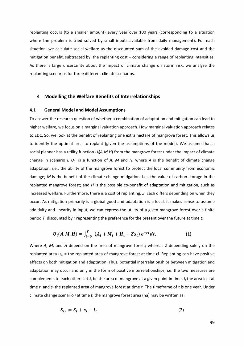
99  

replanting  occurs  (to  a  smaller  amount)  every  year  over  100  years  (corresponding  to  a  situation 

where  the  problem  is  tried  solved  by  small  inputs  available  from  daily management).  For  each 

situation, we  calculate  social welfare as  the discounted  sum of  the avoided damage  cost and  the 

mitigation benefit, subtracted by  the replanting cost – considering a range of replanting intensities. 

As  there  is  large  uncertainty  about  the  impact  of  climate  change  on  storm  risk, we  analyse  the 

replanting scenarios for three different climate scenarios.   

 

4 Modelling the Welfare Benefits of Interrelationships 

 4.1 General Model and Model Assumptions 

To answer the research question of whether a combination of adaptation and mitigation can lead to 

higher welfare, we focus on a marginal valuation approach. How marginal valuation approach relates 

to EDC. So, we look at the benefit of replanting one extra hectare of mangrove forest. This allows us 

to  identify  the optimal  area  to  replant  (given  the  assumptions of  the model). We  assume  that  a 

social planner has a utility function Ui(A,M,H) from the mangrove forest under the impact of climate 

change  in  scenario  i. Ui    is  a  function  of  A, M  and H, where  A  is  the  benefit  of  climate  change 

adaptation,  i.e.,  the ability of  the mangrove  forest  to protect  the  local community  from economic 

damage; M  is the benefit of the climate change mitigation,  i.e., the value of carbon storage  in the 

replanted mangrove  forest; and H  is  the possible co‐benefit of adaptation and mitigation, such as 

increased welfare. Furthermore, there is a cost of replanting, Z. Each differs depending on when they 

occur. As mitigation primarily  is a global good and adaptation  is a  local,  it makes sense  to assume 

additivity and  linearity  in  input, we can express the utility of a given mangrove forest over a finite 

period T, discounted by r representing the preference for the present over the future at time t: 

  

, , ,     (1) 

Where A, M,  and H depend on  the  area of mangrove  forest; whereas  Z depending  solely on  the 

replanted area (st, = the replanted area of mangrove forest at time t). Replanting can have positive 

effects on both mitigation and adaptation. Thus, potential interrelationships between mitigation and 

adaptation may occur and only  in the form of positive  interrelationships,  i.e. the two measures are 

complements to each other. Let St be the area of mangrove at a given point in time, lt the area lost at 

time t, and st the replanted area of mangrove forest at time t. The timeframe of t is one year. Under 

climate change scenario i at time t, the mangrove forest area (ha) may be written as:  

 

,              (2) 

100  

lt  is a  function  (g) of  the current overall area of  the mangrove  forest  (St)  impacted by  the climate 

change (Cit) in the current climate change scenarios (i) at time t: 

 , ,            (3) 

Notice that this implies that we assume that a replanted and an existing hectare of mangrove have 

the same value. Without a spatially‐specific model, this is a reasonable assumption at the margin. 

In the following section, we shall look at how A, M, H, and Z are estimated.  

 4.1.1  The Benefit of Adaptation (A) 

We estimate the increases of welfare benefit by replanting (st). This activity can increase the overall 

area of mangrove forest (St). 

To estimate the ability of the mangrove forest to protect the local community, we use an ‘expected 

damage  function’  (EDF), which will give us  the option of  calculating  the marginal EDC,  taking our 

point of departure  in Barbier  (2007) and Hanley and Barbier  (2009). The EDF  is derived  from  the 

‘production function’ (PF) by which the environment  is valued as an  input  in the creation of assets 

that  increase  the  utility  for  the  local  community.  In  our  case,  the  EDF  describes  the  relationship 

between damage caused by  storm and  the  loss of  the mangrove  forest and,  thereby, production. 

Whereas Barbier (2007) and Hanley and Barbier (2009) deal with a static model, we have a dynamic 

model because this better captures the key attributes of climate change – the continuous change in 

conditions. 

We  use  the  aggregated  households  from  this  study  site  to  represent  the  entire  community  and, 

thereby, the preferences of the social planner. The aggregated households’ expenditure function  is 

expressed as m(P,Ci,Ui).  Ui   is the utility level for a given climate scenario i, and Ui

0 indicates that no 

replanting  is done  in climate scenario  i. Notice that, with climate change, the utility may vary over 

time  and,  thus, will not  reflect  today’s  consumption possibilities.  P  is  a price  vector  for  acquired 

goods consumed by the householdss. Ci represents the impact of climate change under the climate 

scenario i. 

The  EDC,  E[D(C)],  is  the welfare  loss  caused by  changes  in  the  number of  acquired  goods  in  the 

expenditure function, i.e., the minimum income needed to offset the change. This is a result of the 

expected damage to the households due to the shift of C. If we let C0 denote the consequences of a 

‘no  change’  scenario and K(C)  the minimum  income  for a household  to maintain  the  initial utility 

level, then we can say: 

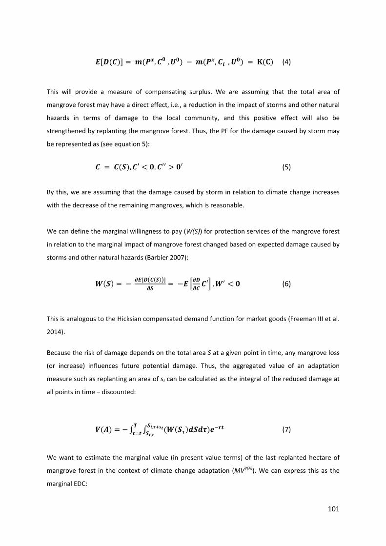
101  

 

, , , ,   (4) 

 

This  will  provide  a  measure  of  compensating  surplus. We  are  assuming  that  the  total  area  of 

mangrove forest may have a direct effect, i.e., a reduction in the impact of storms and other natural 

hazards  in  terms  of  damage  to  the  local  community,  and  this  positive  effect  will  also  be 

strengthened by replanting the mangrove forest. Thus, the PF for the damage caused by storm may 

be represented as (see equation 5): 

  , ′ , ′′ ′          (5) 

 By this, we are assuming that the damage caused by storm  in relation to climate change  increases 

with the decrease of the remaining mangroves, which is reasonable. 

 

We can define the marginal willingness to pay (W(S)) for protection services of the mangrove forest 

in relation to the marginal impact of mangrove forest changed based on expected damage caused by 

storms and other natural hazards (Barbier 2007): 

 

′ ,       (6) 

 

This is analogous to the Hicksian compensated demand function for market goods (Freeman III et al. 

2014). 

Because the risk of damage depends on the total area S at a given point in time, any mangrove loss 

(or  increase)  influences  future  potential  damage.  Thus,  the  aggregated  value  of  an  adaptation 

measure such as replanting an area of st can be calculated as the integral of the reduced damage at 

all points in time – discounted: 

 

,

,        (7) 

 We want  to estimate  the marginal value  (in present value  terms) of  the  last  replanted hectare of 

mangrove  forest  in  the context of climate change adaptation  (MVV(A)). We can express  this as  the 

marginal EDC:    

102  

 

             (8) 

 

4.1.2 The Benefit of Mitigation (M) 

The benefit  of mitigation  is  calculated  as  the monetary  value  of  the  carbon  sequestration  in  the 

replanted mangrove  forest at  time  t, as  the  trees  sequestrate CO2  from  the air and  capture  it as 

carbon in the wood. From a social planner perspective, the monetary value could be seen as the SCC.  

The benefit of mitigation at time Mt can be expressed as a function of  over the time period we are 

considering:  

 

,               (9) 

 

where L is the function for captured CO2e in the mangrove forest. 

This can be rewritten as equation 10; St  is reduced out of the function, since we are assuming that 

the  existing mangrove  forest  is  a  closed  system  that  does  not  contribute  any  additional  carbon 

sequestration or emission. The mitigation benefit will be calculated on basis of the area of mangrove 

forest lost at time t (lt) and the replanted area at time t (st):  

 

             (10) 

 Aggregating and discounting over  time, we have  the contribution  to equation 1, and  the marginal 

value of mitigation can be obtained in a manner similar to equation 8 for adaptation.  

 

4.1.3 Co‐benefits in Relation to Replanting the Mangrove Forest (H) 

The  benefits  that  are  achieved  in  addition  to  the  benefits  of  climate  change  adaptation  and 

mitigation  are  referred  to  as  the  co‐benefits of  replanting  the mangrove  forest  (see  equation 1). 

These co‐benefits are related  to the  increased welfare that may be a result of an  improvement of 

the breeding conditions and  the natural habitat  for  fish, dolphins, coral, etc.,  for  this specific case 

study.  It  is a welfare gain because of the enhanced economic activities that are dependent on the 

mangrove forest for the local community/fishery and tourism. The case we are considering is coastal 

fishery and open access fishery. Therefore, the fishery in the area is not optimally managed and also 

suffers from unsustainable fishing. The consequence of open access is that, if any profit is apparent, 

103  

it will draw the attention of new fishermen, who will then establish themselves  in the community, 

which will equalise any producer surplus. However, it will still affect the welfare through its influence 

on  consumer  surplus  (Barbier  2007).  We  are  assuming  that  the  co‐benefits  are  positive  and 

increasing with St. However, the data required to estimate the  influence of co‐benefits  is  limited  in 

our case. Therefore, they are assumed to be zero (Ht=0) in our case study, but the model could easily 

be expanded.  

 

4.1.4 Replanting Costs (Z) 

The cost of replanting the mangrove area, Z, is assumed to be constant per hectare. We assume that 

the  cost  of  replanting  the  mangrove  forest  as  an  adaptation  initiative  is  equal  to  the  cost  of 

replanting mangrove  forest  as  a mitigation  initiative.  Thus,  if  the  cost has been  accounted  for  in 

estimating  the  benefit  of  adaptation,  it  will  not  be  necessary  to  account  for  the  cost  again  in 

estimating the benefit of mitigation.  

 

4.2 Simulation  

With the utility function described above and specification of the components, we can now describe 

the  simulations  performed.  To  analyse  the welfare  consequences  under  different  scenarios  and 

strategies for adaptation to and mitigation of climate change, we are operating with three damage 

scenarios  and  two  replanting  strategies.  We  carried  out  the  simulations  in  the  MATLAB2013 

environment. 

 

4.2.1. Damage Scenarios as a Consequence of Climate Change  

When  the wind speed reaches 12 m/sec, damage occurs  (CCCA 2012). Therefore,  in the  following, 

we shall refer to this as a storm even  if  it  is not defined so  in technical terms. From 1979 to 2012, 

wind speeds over 12 m/sec were measured at two points outside Cambodia's coast. These historical 

data  have  provided  us with  an  opportunity  to  calculate  the  daily  probability  of  storms  for  each 

month of each year (Nielsen 2013).   It  is sometimes argued that storm frequencies and strength  in 

some  locations will  increase.  However,  according  to  IPCC  5th  assessment  report  (Hijioken  et  al. 

2014), there is currently no indication that the frequency of storms will increase or decrease off the 

coast of Cambodia; however, coastal and marine systems will suffer from climatic and non‐climatic 

drivers, as strength and impacts of storms. Therefore, we base our simulation on the historical data, 

simulating day‐specific risk of wind speeds higher than 12 m/sec for a 100 year period. Developing 

three damage scenarios  illustrating how the PF for a damaged mangrove forest will develop under 

104  

the  influence of the storms. The PF  for the damage scenarios, equation  (5),  is partly based on the 

assessment of the destroyed mangrove area in Peam Krasaop from 2011(CCCA 2012), assuming that 

ecosystem services do not respond linearly to changes in habitat size (Barbier et al. 2008).    

To comply with the uncertainty regarding the expected climate change for the study area, and that 

no detailed  data  exist,  consequently we  set up  three  scenarios  that  can  demonstrate  a  range of 

possible  changes.  The  first  is  a  baseline  scenario,  reflecting  the  climate  of  today;  the  second 

contemplates greater destruction; whereas the third has stronger storm occurrences once in a while, 

damaging the resilience of the system. The three damage scenarios are described by equation 11:  

∗ ,            (11) 

      

Damage Scenario 1: Is based on our knowledge of storm occurrences in 2011, and we simulate the 

start of the first storm by removing 0.08 ha of mangrove forest, based on equation 11, where a = ‐

0.001770 and b=5. This  reflects an almost  ‘no change’ scenario  (as compared  to  today). However, 

the amount of mangrove  forest  removed per storm  increases slowly but exponentially because of 

the assumption made in equation 5. 

Damage Scenario 2:  Is based on  that 1 hectare of mangrove  forest will be  removed each  time  a 

storm occurs to start with, and then it develops exponentially. Equation 11 was fitted based on this 

assumption: a = 0.00099 and b=10. The destruction of the mangroves develops exponentially. 

Damage Scenario 3: Is based on damage scenario 1 and an obstruction of, for each 30 storms, one 

typhoon will occur. The  typhoon  is assumed  to destroy 50 ha of mangrove  forest each  time. The 

typhoon’s destruction of  50 ha  is not  influenced  by  the  replanting  strategies of mangrove  forest 

under the simulation, as damage scenarios 1 and 2 are. The simulated typhoon’s destruction reflect 

a severe incident but without causing complete destruction.   

Figure 1  shows how  the  three damage  scenarios will destroy  the existing 2,324.4 ha of mangrove 

forest over time, assuming there is no replanting to delay the destruction. Under damage scenario 1, 

the destruction is minimal compared to damage scenario 2 in which everything will be destroyed by 

year 60 and damage scenario 3 in which everything will be destroyed by year 63. The reason the two 

curves  cross  is  that  the  obstruction  in  damage  scenario  3  over  time  delays  the  total  destruction 

compared to damage scenario 2. From around year 50, damage scenario 2 start to go beyond 50 ha 

of destruction. It is assumed that no regeneration of the storm‐damaged areas will occur. 

 

105  

 Figure 1 the destruction of the mangrove forest from year 1 to 100 in the three damage scenarios without any replanting of the mangrove forest.   

 4.2.2. Replanting Strategies  

We operate with two replanting strategies for adaptation that differ in terms of the time when the 

replanting occurs.  The  replanting  strategies  are meant  to  reflect  two  extreme  approaches. While 

early replanting is, ceteris paribus, favoured compared to later because of the increasing destruction 

rate,  it may  not  always  be  feasible  due  to  limitations  in  the  availability  or  access  to  knowledge, 

capital, and labour. The two replanting strategies for simulations are defined as follows: 

Replanting Strategy A: One‐shot replanting of mangrove forest at intervals of 1 ha from 0 to 500 ha, 

where replanting is only carried out in year 1 of the 100 year period of the simulations. This reflects 

the fastest possible action.   

Replanting Strategy B: Continuous replanting of mangrove forest at intervals of 0.25 ha from 0 to 15 

ha, where  replanting  is  carried  out  each  year  in  the  100‐year  simulation  period.  This  reflects  a 

situation  in which, e.g.,  labour availability  is  limited and,  therefore,  constrains  the magnitude per 

year. 

 

4.3 Data and Functional Forms 

In  this  section, we  describe  the  data  and  various  assumptions  for  the  concrete  simulation.  The 

Cambodia Climate Change Alliance (CCCA) carried out a vulnerability assessment of the community's 

risks  from  climate  change  in 2012.  The CCCA obtained data  through  informal questionnaires  and 

facilitated group discussions with  the communities concerned.  In  January 2014, we visited  the 15‐

106  

hectare replanting site and the community of the fishermen just outside the city of Koh Kong in the 

Peam Krasaop Wildlife Sanctuary. Exploratory  interviews with fishermen and other member of the 

community  were  conducted  in  which  the  information  obtained  through  the  CCCA  (2012)  was 

confirmed. For  the  simulations,  the  replanted mangrove area  is assumed  to be  located  inside  the 

Peam  Krasaop  community  border.  Areas  in  which  climate  change  is  having  an  impact  on  the 

mangrove forest were also visited along with two park rangers and an interpreter. Information about 

cost  and  expenses  in  relation  to  the  replanting  site  was  also  obtained  through  the  project 

coordinator  (VAAP  LDCF  2013)  along  with  additional  information  about  the  fishermen's  use  of 

equipment, commodities, and belongings (Nielsen 2014).    

 

4.3.1 Replanting Cost 

The cost of replanting was obtained through the CCCA, which was responsible for replanting the 15 

ha  of mangrove, costs include gathering seeds for new plants, renting boats, hiring people from the 

community for seed‐gathering and planting mangrove seedlings, monitoring, and later replanting, if 

necessary. The cost also include an event to raise awareness of the project in the community (CCCA 

2012). The cost does not include soil preparation. The total cost of replanting 15 ha was USD 16,441 

(or USD  1,096  per  hectare).  The  cost  of  replanting  the mangrove  forest  used  in  the  simulation, 

excluding the awareness event, is estimated to be USD 896 per hectare.  

 

4.3.2 EDC 

The annual EDC is calculated based on the income lost. Thus, apart from the information on the area 

of damaged mangrove depending on  the  remaining area, we also need  information of household 

income  and  assets.  The  277  households  in  the  community  can  be  divided  into  three  different 

categories of poverty, where 51% belongs to the two poorest groups2. The community’s aggregated 

income as USD 445,416 per year (CCCA 2012).  

To assess the annual damage costs as a function of remaining mangrove, data from tree situations 

were considered. The first one is an estimated cost of USD 49,4003 of storm damage in 2011 where 

2023  ha mangrove was  left  (CCCA  2012).  The  second  one  is  an  estimation  of  the  loss  of  a  total 

destruction of the community, which we assume will occur when 2/3 of the mangrove is destroyed 

                                                       2 the two lowest income groups are characterized by not having their own home, living on land illegally, having their own house but very far from the main road or having a very low income but living close to the main road (CCCA 2012). Other indicators of these groups are that they have lost family income, faced food shortages, have sold properties, or borrowed money from people within the last 12 months (CCCA 2012). 3 This is an aggregated value for the whole community. It is biased towards the poorer income groups due to their low‐quality houses and boats. 

107  

(770 ha is left). Here the fishing options present around the mangrove forest are no longer assumed 

sufficient  to  sustain  livelihood. The  average household earns 1608 USD/year  (CCCA 2012),  so  the 

aggregated  income for the 277 households  is USD 445416. Adding the value of their assets4 (taken 

from (Nielsen 2014), results  in a  loss of UDS 1.2 million. Finally, we use a  lower bound estimate of 

damage of USD 1,800 as it is unlikely that storm damage can be completely avoided because of the 

poor quality of houses and boats. Based on these three points, an exponential function of the EDC 

depending the area (ha) of mangrove forest remaining each year is estimated as:   

∗               (12) 

 

where c = 14,726,276.0915 and g = ‐0.00291. To avoid extraordinary large damage costs when little 

mangrove is left, we set an upper boundary of USD 1.6 million. 

The expected damage cost  is calculated on an annual basis. When no mangrove  is  left,  livelihood 

options corresponding to the annual income are lost – every year, forever. This is of course only true 

to the extent that people cannot move away and find other ways to sustain themselves. In the other 

extreme, we  can  assume  that  they  just  find  another  living,  and  thereby  there  is  no  income  loss 

present  once  people  move  away.  Given  the  limited  livelihood  options  in  the  area,  and  the 

importance of the mangrove not only in this village but for larger areas, this may also be unrealistic. 

Consequently, we use  the one  extreme  –  calculating  the  annual  loss  as present  every  year  after 

destruction. The other extreme, zero cost once the mangrove  is destroyed was also calculated but 

results are not shown. But we will refer briefly to these results in the result section. 

 

4.3.3 Calculating Carbon Sequestration under the Influence of the Damage Scenarios and 

Replanting Strategies  

The IPCC tier 1 guidelines have been used (IPCC 2014a; IPCC 2006) to estimate the possible carbon 

sequestration and emission  in  the mangrove  forest, with  respect  to  the  remaining,  replanted and 

damaged mangrove forest. 

                                                       4 This is not equally distributed. But as we work with aggregated values, the distributional aspect does not matter for the estimation. 

108  

The  area of mangrove  forest destroyed under  the  three damage  scenarios will  count  for  the  full 

destruction  in  the year  it occurs,  creating an emission of 129  tonnes of  carbon per ha/year  (IPCC 

2014a). 

The time span for calculating the carbon sequestration in the replanted mangrove forest is based on 

Alongi  (2008).  Alongi  (2008)  uses  long‐term  data  from  French  Guinea,  which  indicates  that  a 

mangrove  forest  stand  follows  a  series of  successive  stages:  rapid  early development,  a maturity 

stage,  and,  finally,  a  stage  of  senescence  in  which  the  stand  breaks  down  and  a  new  stand  is 

regenerated  and  colonised.  In  the  calculation  of  the  possible  carbon  sequestration, we  limit  the 

influence of gap dynamics only to consider how much of the mangrove forest is left in each scenario 

of the simulations.  

At  first,  the  replanted mangrove  forest will  create carbon emissions of 1.62  tonnes ha/year  (IPCC 

2014a), this stage of rapid early development will lasts five years (Alongi 2008; Fromard et al. 1998). 

After  that,  the  replanted mangroves will  reach  the maturity stage and create sequestration  in  the 

amount of  6.65  tons  carbon ha/year  (IPCC  2014a), which we  estimate will  last  approximately  65 

years in the replanted area (Alongi 2008).  

Replanting strategy B  in which replanting  is done every year will contribute consistently  to carbon 

sequestration  from  year 6 until 0 ha  is  left, but  the  act of  replanting will only be done until  the 

threshold of 770 ha  left mangrove  forest  is  reached. However, even  if  the  threshold of 770 ha  is 

reached, CO2 emission will continue from mangrove destruction until 0 ha mangrove  is  left none  is 

left. 

Human  collection of  fuel wood  and other wood  removal  leading  to deforestation  should  also be 

included in the estimation of the carbon sequestrated for the area. Data availability on this subject is 

very poor for the Peam Krasaop community. Therefore, the net emissions from fuel wood and wood 

removal have not been included in the calculation.  

The  benefit  of  climate  change  mitigation  is  estimated  on  the  basis  of  the  amount  of  carbon 

sequestrated and converted to tons CO2‐equivalent (tCO2e) under the constraints and assumptions 

mentioned  above  for  the  calculation  of  the  amount  of  tCO2e, which we  then  assign  a monetary 

value. We are using three different CPs to give the carbon sequestration a monetary value; we use 

prices from existing markets, to reflect what  local decision‐makers will take  in to account. The first 

CP  (CP1)  represents  the  price  for  the  ‘certified  emission  reductions’  (CERs)  under  the  ‘clean 

109  

development mechanism’  (CDM),  under  the  Kyoto  protocol.    The  price  for  trading  CERs  on  10 

February 2014 was USD 0.545 per tCO2e (Fenhann 2014). The second carbon price (CP2) refers to the 

social cost of tCO2e. We apply the very low SCC price of USD 6.8 per tCO2e, referring to Tol (2008)6, 

who bases this estimate on over 200 estimates of the SCC. The third CP (CP3) is the average price of 

CERs traded between 21 May 2007 and 10 February 2014 (Fenhann 2014), which is EUR 9.66 or USD 

13.18  (XE 2014).   The CPs are multiplied by  the amount of  tCO2e sequestrated or emitted  for  the 

specific year and  in  the specific  replanting stage  for each of  the  replanting strategies and damage 

scenarios.  Therefore,  they  will  have  a  negative  monetary  value  if  more  CO2e  is  emitted  than 

sequestrated. Appendix C illustrates the consequence of SCC in the range of USD 50‐200 (not part of 

the submitted paper). 

   4.3.4 Calculation of the Marginal Value of Climate Change Adaptation, Mitigation and 

Replanting Cost  

If  we  know  the  annual  EDC  for  the  three  different  damage  scenarios  combined  with  the  two 

replanting  strategies,  including  the  cost  of  replanting  for  each  adaptation  initiative,  and  the 

monetary  value  of  the mitigation  initiative  (carbon  sequestrated  and  emitted  in  the  mangrove 

forest), it is possible to calculate the present value of each adaptation and mitigation initiative under 

each of the replanting strategies. In this way, we can calculate the expected marginal EDC for each 

replanting  and  damage  scenario  and,  thereby,  evaluate  the  different  strategies.  To  reflect  the 

preference  for the present over the  future, we made the simulations with  four7 different discount 

rates: 4% and 12% is presented in the paper. This reflects the choice that the decision‐makers have 

to take, and what priorities they have (Arrow et al. 1996). The four discounts rates contribute to a 

sensitivity  test of  the  expected marginal  EDC  for  each  replanting  and  damage  scenario. Discount 

rates at 4% or  lower reflect a private planner or an alternative  investment  in a developed country, 

whereas 12% or higher reflect the private actor  in a developed country. Specific for Cambodia can 

the discount rates for micro‐loans reach 2‐3.5% per month, cumulative equivalent to close to 50% 

per annum (CCCA 2012).  Therefore, the discount rate most commonly used in developing countries 

is applied.  

For each damage scenario and replanting strategy (and discount rate), we first calculate the present 

value of the cash flow of the EDC. Then, we summarise the present values over the 100‐year period 

                                                       5 The CP for CERs on February 10 2014 was EUR 0.40 (for exchange rates, see XE (2014)). 6 Converted to tCO2e from his reporting of USD 25 per tC 7 The marginal EDC and mitigation values in relation to the replanting cost under influence of 2% and 20% discount rates is available in Appendix B.  

110  

in each of  the different  stages of  the  replanting  strategies. This  is used  to  calculate  the marginal 

value  as  given  by  equation  8.  Because  storms  are  random,  the  exponential  development  of  the 

strengths  and  destructive  power  of  the  storms  in  the  three  damage  scenarios,  the  estimated 

expected  damage,  is  not  smooth.  So,  to  calculate  the  slope,  different  approaches  were  used, 

depending on what fitted best. The model fitted for the adaptation under the replanting strategy A 

was a  two‐term exponential  function by which  the derivative  function gives  the marginal value of 

one extra ha mangrove forest replanted. This fitted poorly for adaptation, mitigation and replanting 

costs8 under replanting strategy B and mitigation under replanting strategy A. So, here, we used a 

moving average of 5 adjacent points of the present value, where the marginal value is found as the 

difference between two adjacent points of the moving average.  

 

5  Results 

 

5.1  Annual Values for Adaptation and Mitigation 

In  this  section, we will  first present  the annual EDC, At,  for  the adaptation  strategy  for  replanting 

strategies A and B, and the corresponding annual mitigation benefit (figures available in appendix A), 

Mt for the 100 year periode that we run the simulations over. These form the basis for the marginal 

curves for EDC and CP1, CP2, and CP3, which may be compared with the marginal replanting cost. 

Figure 2 below shows the annual EDC, At, over time for replanting strategy A at three different levels 

of replanting ‐ 0 ha, 250 ha, and 500 ha ‐ and for the three different damage scenarios. It is seen that 

At  increases over time as fewer mangroves remain but also that replanting delays destruction and, 

thereby,  increases  At. When  the  forest  is  total  destroyed,  At  will  be  equal  to  USD  1.6 million, 

corresponding  to  the  opportunity  cost  of  the  mangrove  forest  and  the  communities  complete 

destruction. Under damage scenario 1, At  is  low compared  to  the  two other damage scenarios.  In 

fact,  it  is close to zero, and total damage will not occur. If replanting  is done, At decreases from an 

average of USD 21,015 at 0 ha to USD 9,847 at 250 ha and USD 4,997 at 500ha – a change that is not 

visible  in  figure2.  In damage  scenario 2,  total destruction will occur  in  year 52  if no  replanting  is 

done,  and  replanting  250  and  500  ha,  respectively,  may  postpone  this  for  17  and  37  years, 

respectively. For scenario 3, total destruction will occur in year 51, and replanting 250 or 500 ha may 

                                                       8 Notice that, because replanting in scenario B occurs over time, the marginal cost of one extra hectare is not constant – e.g., replanting stops in the scenarios when the mangroves are completely destroyed. 

111  

postpone this for 10 and 18   years, respectively. Thus, the more severe the damage, the smaller  is 

the effect of major replanting now.    

Figure 3 shows a similar picture as figure 2, just for replanting strategy B. For replanting strategy B, 

the  replanting  cost  is  incurred  each  year  as  the  mangroves  are  replanted  until  only  770ha  of 

mangrove forest are left. The no‐replanting strategies are identical to Figure 2, and we also find that 

replanting under damage scenario 1 has a small effect, though larger than under replanting strategy 

A. In damage scenario 2, replanting 15 ha per year may delay the increase in annual damage cost, so 

that  total destruction  is not reached. For damage scenario 3, replanting 15 ha a year will result  in 

total destruction in year 89. The overall the picture for figure 3 is that replanting delays the increase 

in At  and that replanting of 15 ha  a year makes a significant difference in this regard, especially  in 

damage  scenario 2  in which  the mangrove  forest  is not destroyed within  the 100‐year  simulation 

period.     

The  results  for  the annual mitigation values show  that,  for  replanting strategy A  for all  three CPs, 

damage scenario 1 has a positive mitigation value  from year 6 to 76. After year 76, the mitigation 

value becomes slightly negative, which  is caused by  the  limited destruction of mangrove  forest  in 

damage scenario 1 and further slowed down due to the termination of replanting.  For the damage 

scenarios 2 and 3, it is clear that the destruction of the mangrove forest has a negative impact on the 

annual carbon sequestration (see figure A1, A3 and A5 available in appendix A). 

Mitigation  values  for  replanting  strategy  B,  damage  scenario  1,  is  the  one  less  influenced  by 

destruction, whereas damage scenarios 2 and 3 are both heavily influenced by the destruction of the 

mangrove  forest, which creates a  large amount of emissions  that  influence  the monetary value of 

mitigation negatively. Similar to the annual damage costs (At)(figures 2 and 3),  it  is possible to see 

that replanting has a significant influence on the mitigation in damage scenarios 2 and 3, as it delays 

the point of complete destruction. When no forest is left, no carbon is sequestrated or emitted (see 

figure A2, A4 and A6 available in appendix A).     

  

112  

         

 Figure 2.  Simulated annual expected damage cost, At (x‐axis), over the 100‐year period (y‐axis) for replanting strategy A and three different levels of replanting (0 ha, 250 ha, and 500 ha) influenced in the three damage scenarios.   

 

 Figure 3 Simulated annual expected damage costs, At (x‐axis), over the 100‐year period (y‐axis) for replanting strategy B and three different levels of replanting (0 ha, 5 ha and 15 ha) influenced in the three damage scenarios. 

 

5.2  Marginal Values 

Figure 4 shows the aggregated present value of damage costs as the marginal EDC (i.e., the damage 

costs avoided by replanting one more hectare) at a discount rate of 4% for replanting strategies A 

and B along with  the present value of  the marginal mitigation value   and  the marginal  replanting 

113  

costs  at  the  three CPs. We  see  that,  for both  replanting  strategies,  the marginal  EDC  in damage 

scenario  1  is  around  the  same  size  as  the marginal  replanting  cost  –  they  intersect  at  68  ha  for 

replanting strategy A and 2.25 ha for replanting strategy B. However, if mitigation is included, it will 

be worth doing the replanting.  If the price  is high (CP2 or 3), the curves never  intersect; but,  if the 

price  is  low,  we  see  that  looking  at  mitigation  and  adaptation  jointly  will  lead  to  an  optimal 

replanting of 209 ha in replanting strategy A and 5 ha per year in replanting strategy B. For damage 

scenarios 2 and 3, the EDC is well above the marginal replanting cost. So, replanting is beneficial. If 

mitigation were considered as a single product, it would only be worthwhile to do replanting if prices 

were above the low price scenario (CP1). A similar pictures may be seen if we apply a discount rate 

of 2% (see appendix B, figure B1). 

 Figure 4 The marginal avoided EDC for the two replanting strategies A and B (adaptation initiatives) in each of the three damage scenarios (the black solid lines with dots), together with marginal mitigation values for the three CPs: CP1 = USD 0.54 per tCO2e, CP2 = USD 6.8 per tCO2e, CP3 = USD 13.18 per tCO2e (the dashed lines). The thin black line shows the marginal replanting costs. All assume a discount rate of 4%. 

114  

These results assume a 4% discount rate –reflecting the discount rate of a social planner. A higher 

discount  rate might  reflect  the decisions of a private actor –  if  incentives are provided  for public 

good mitigation. Figure 7 shows the results for a 12% discount rate. Here, we see that,  in damage 

scenario 1, the marginal EDC is considerably below the marginal replanting costs, and only CP2 and 

CP3 are high enough  to  justify replanting.  In damage scenarios 2 and 3, however, we see that  the 

EDC and  the  replanting  cost  intersect,  so  that,  looking at adaptation alone  in damage  scenario 2, 

optimal  replanting  intensities  are  243  ha  under  replanting  strategy  A  and  10  under  replanting 

strategy B.  In damage  scenario 3, we  see  that,  for  replanting  strategy B,  replanting more  than 15 

ha/year is optimal; whereas, for replanting strategy A, the optimal replanting is 132, i.e., below the 

optimal for damage scenario 2. This is because the benefit of replanting is higher in damage scenario 

2. This can also be seen from Figure 2, where the integral of the difference between replanting 250 

ha and 500 ha is larger in damage scenario 2 than damage scenario 3.  

Looking at mitigation, we see that, for the lower discount rate, price scenarios CP2 and CP3 pay off 

the replanting costs fully – it is more pronounced than for lower discount rates. If the discount rate 

is increased to 20%, the replanting costs exceed the mitigation values (see appendix B, figure B2).  

 

115  

 Figure 5 The marginal avoided EDC for the two replanting strategies A and B (adaptation initiatives) in each of the three damage scenarios (the black solid lines with dots), together with marginal mitigation values for the three CPs: CP1 = USD 0.54 per tCO2e, CP2 = USD 6.8 per tCO2e, CP3 = USD 13.18 per tCO2e (the dashed lines). The thin black line shows the marginal replanting costs. All assume a discount rate of 12%. 

Two assumptions are crucial for the above shown results, namely the choice of assuming continued 

loss once  the mangrove  is  left, and  the  choice of using  relatively  low  carbon prices  compared  to 

many  of  the  SCC  estimates which  should  be  used  in welfare  economic  analyses.  Assuming  that 

people  just  find other  livelihood options  if  the mangrove  is destroyed would  reduce  the expected 

damage cost.  In the case of a 4% discount rate this would still result  in the expected damage cost 

being  larger  than  the  replanting  costs  for damage  scenario  2  and  3.  For  a  discount  rate of  12%, 

damage scenario 2 and replanting strategy A, the EDC and the replanting costs, would intersect each 

other  at  220  ha,  i.e.  around  100  ha  less  than  in  the  scenarios  shown.  For  the  corresponding 

replanting strategy B, the benefits from around 8 ha of replanting will offset the costs.  This pattern 

is repeated for the other scenarios. Consequently, while the area optimal to replant  is reduced, an 

effort  is still beneficial. And  if mitigation benefits are  included  it  is even more so. This  leads to the 

116  

second  sensitivity  –  namely, what  is  a  high  SCC  of  carbon was  used:  in  that  case,  it  would  be 

beneficial  from  a welfare  economic  point  of  view  to  replant  the maximum  area  analysed  for  all 

scenarios. 

 

6 Discussion 

 

 6.1   Main Findings  

The  aim  of  this  paper  was  to  analyse  the  interrelationships  of  the  benefits  of  climate  change 

adaptation and mitigation. We do so by  looking at the marginal value of replanting  in a small case 

study in which causes and effects are visible and, thereby, possible to interpret in a broader context.   

The  overall  assumption  is  that  there  is  a  joint  benefit  from  climate  change  adaptation  and 

mitigation;  thus,  they  complement  each other.  From  a  social planner’s point of  view,  adaptation 

alone  makes  replanting  mangroves  beneficial  as  the  adaptation  benefits  are  larger  than  EDC. 

Mitigation emphasises this. Our results show that even for the highest replanting intensities we have 

analysed  (500  ha  from  the  beginning  or  15  ha  per  year  over  100  years),  replanting  is worth  the 

effort.  If  the discount rate  is high, 12%, we  find  that adaptation by replanting  is only beneficial  to 

some extent –  in damage scenario 2, replanting 250 ha from the beginning or 10 ha per year over 

the next 100 years is optimal, and in damage scenario 3, replanting 140 ha from the beginning or 15 

ha per year over the next 100 years. So,  in conclusion, the study shows that,  looking at adaptation 

alone only makes replanting the mangroves worth the effort if increases in storm frequency occur. If 

mitigation  is  included,  prices  as  low  as  in CP2  (6.8 USD per  tCO2e) makes  the highest  replanting 

intensity  worth  the  effort.  Consequently,  looking  at  both  adaptation  and  mitigation,  makes 

replanting worth  the effort even  if  there  is no  increase  in  storm  frequency. Notice  that  this  cost 

estimate is well below most estimates of SCC. van den Bergh and Botzen (2014) indicate that an SCC 

should  not  go  below  USD  125  per  tonne  CO2e.  Applying  such  high  values would  just make  the 

emphasis  on  including  mitigation  in  adaptation  more  pronounced,  as  the  marginal  mitigation 

benefits in Figures 4 and 5 would be very much above the marginal replanting cost (see Appendix C, 

not part of  the submitted paper).  If we are  thinking of paying  for carbon sequestration  through a 

market price in a carbon emission trading scheme, it is much more likely that we lie in the lower end 

of CPs – unless there is political will to have the amount of quotas to reflect the SCC.  

From a private decision maker’s point of view, only adaptation is relevant – unless mitigation is paid 

for. And a higher discount rate would very  likely also apply.  In the study here, we operated with a 

117  

12% (real) discount rate; and, in that case, the area it would be optimal to replant would be smaller 

than  in  the  social  planner  case  for  all  damage  scenarios.  However,  if  payment  for mitigation  is 

implemented  to  reflect  an  increase  in  public  good  provisions  together  with  the  adaptation 

component, replanting would still be optimal – also from a private decision maker’s point of view.  

An increase to 20% makes the whole thing a bit more impervious for investors, since the replanting 

cost exceeds the marginal benefits of mitigation and the EDC.  

Comparing  the  two  replanting  strategies, we  see  that,  if we  assume  that  storms  always destroys 

mangroves, a continuous replanting (replanting strategy B) may,  in many  instances, be beneficial – 

as  it can halt ongoing destruction. Replanting strategy A delays destruction of  the mangrove. But, 

will still lead to total destruction. Consequently, a mixture of the two strategies is probably best – a 

large replanting initially to reduce the risk level and, then, continued replanting of what is destroyed 

to make sure that the high risk levels are not reached again. 

Boutweel and Westra  (2015) argue  that  the values  revealed by  the EDC method are at  the  lower 

boundary compared to other ecosystem valuation methods. Consequently, the adaptation estimates 

in this study may be considered conservative, even though we do not consider alternative livelihood 

options.  

   6.2  Policy Implications 

The complexity of climate change will also need a complex response; a benefit from  implementing 

both adaptation and mitigation is shown, and a mix of the two replanting strategies is suggested.   

A mixture of  the  two  replanting strategies  is suggested as  the optimum  for  interlinkages between 

adaptation and mitigation  from a social planner perspective,  thereby reducing risk by replanting a 

large area to start with and then continuously replanting to maintain the acquired  level of reduced 

risk. If payment for mitigation were included, this might motivate private investors to pledge money 

to replant  in a manner similar to replanting strategy A. The  investment should avoid being a "one‐

time wonder" in which the level of risk reduction from adaptation is seen long before the impact of 

climate  change. By  creating  a mixture of  the  replanting  strategies,  it  is possible  to  see  long‐term 

results  from the  investment, enforced by  including stakeholder  involvement and awareness of  the 

mangrove  forest  and  climate  change.  This  could  create  the  motivation  for  the  community  to 

continue  replanting  the mangrove  forest  (similar  to  replanting  strategy  B)  and  strengthen  their 

resilience to climate change by learning to recognise the importance of natural resources to sustain 

their livelihoods, an aspect already reflected in the high replanting costs from the CCCA project. This 

118  

is  an  investor opportunity  to  signal  social  responsibility  that would be beneficial both  locally  and 

globally and, from a long‐term perspective reduce risk. 

The arguments for pursuing both climate change adaptation and mitigation for maximising welfare, 

is reinforced by that there is a limit for climate change adaptation, therefore a threshold for the mix 

of adaptation and mitigation (Watkiss et al. 2015). If climate change exceed this threshold, the cost 

of adaptation will only be a burden to future generations (Laukkonen et al. 2009). This enhances the 

arguments for the mixture of replanting strategies suggested, since the benefits of both adaptation 

and mitigation will have the large impact now but secure future risk reduction on a local scale.  

Laukkonen  et  al.  (2009)  argue  that  local  stakeholders  should  be  persuaded  to  enhance  their 

response  to  climate  change.  To  do  this,  not  only  academic  information  but  also  the  empirical 

knowledge ‐ such as fishermen's knowledge about tidal water and the mangrove forest ‐ is needed. 

From the exploratory interviews of fishermen in Peam Krasaop, it was easy to track awareness of the 

mangrove forest, since the forest sustains their  livelihoods. However, there  is a  large gap between 

this awareness and the knowledge of how they could participate in protecting the mangrove forest 

and the co‐benefits they derive from it. For example, when the tide is high, fishing is possible in the 

replanted area, so boats propellers destroy new seedlings, which delays the developing of the newly 

planted seedlings. Laukkonen et al. (2009) underline that stakeholder  involvement should not be a 

top‐down process but a process that strengthens the feeling of collective responsibility. Through this 

process,  it will also be possible to address other factors that cause damage and degradation to the 

mangrove  forest.  For  example,  the  community  has  recognised  the  income  opportunities  from 

tourists visiting  the mangrove  forest. This  is an  important  issue  to address  since  the  fight against 

climate change is not always the first priority among local communities (Warren et al. 2012; McGray 

et al. 2007). Therefore, it is  also important to support sustainable development, which is necessary 

since climate change will continuously provide challenges (Laukkonen et al. 2009). The use of  local 

initiatives may, in the long run, strengthen and reinforce regional or national strategies (Laukkonen 

et al. 2009).   

This strengthens the argument to pursue climate change adaptation and mitigation simultaneously 

from  a  social  planner  perspective.  For  this  specific  case,  one  could  argue  that  adaptation  and 

mitigation  are  complementary  but  with  a  known  contradictory  example  (Matocha  et  al.  2012; 

Laukkonen et al. 2009):  it  is easy to  imagine situations with a free‐rider effect  ‐ fishermen who do 

not participate in the replanting or who damage newly planted seedlings. Once again, this underlines 

the need to make awareness and sustainable development a part of the adaptation and mitigation 

project.       

119  

 6.3  Caveats  

This paper  is based on a  case  study  in Cambodia  in which data have been  collected  from  locally‐

available  knowledge.  The  quality  of  such  an  approach  lies  in  its  connection  to  decisions  actually 

being taken. It can also be seen as a starting point for stakeholder involvement. However, there are 

some  obviously  caveats  to  the  estimation.  The  economic  data  are  based  on  the  best  available 

knowledge, and it is not considered whether, e.g., replanting costs could be lower. Another element 

it would be relevant to include is other threats from climate change ‐ especially, rising sea levels but 

also temperature increases and changes in precipitation. Adapting to an increased number of storms 

may be worthless  if  the mangrove  forest  is  flooded by  rising  sea  levels. However,  for  the current 

study, this data was not available. Therefore, we leave it to future research. 

The EDC approach is also  applied in large climate change models and IAM (Warren et al. 2012) such 

as the RICE and DICE models (Nordhaus 2014; Nordhaus 2011). An advantage of using  it on a  local 

scale, such as here, is that its limitations become quite clear: results are not better than the data and 

assumptions behind them. Nevertheless, using it at a local level, where processes are clear, makes it 

possible  to  identify  drivers  affecting  the  trade‐offs  between  costs  occurring  now  and  damage 

avoided  in  the  future.  In  the current case,  it has been demonstrated  to be highly  sensitive  to  the 

intensity of  storm  risks. Another consequence of  the assumption  is  that  replanting  strategies  that 

are not continuous will,  in the  long run,  lead to destruction. While this may be correct  in the near 

future, one could hope that, as the ecosystem becomes resilient, it will no longer be the case.   

    

7 Conclusion 

  Methodological  developments  for  handling  the  interrelationships  between  climate  change 

adaptation  and  mitigation  demand  innovative  thinking.  The  paper  combines  general  economic 

theory  with  case‐specific  knowledge  obtained  from  stakeholders,  contributing  with  empirical 

knowledge.  This  paper  is  a  step  on  the way  towards  developing  a methodology  to  estimate  the 

interrelationships between  climate  change adaptation and mitigation. Thus,  it  illustrates how, we 

can evaluate different strategies for adaptation and mitigation.   

This case from Cambodia shows that, from a social planner perspective, there are positive benefits 

from  replanting  mangroves  taking  only  adaptation  into  consideration  but  even  more  when 

mitigation  is  included.  Consequently,  looking  at  adaptation  and mitigation  jointly  leads  to  higher 

120  

replanting  intensities  than  looking  at  adaptation  alone.  For  this  to motivate  for  private  decision 

makers to pledge money for investment, payment for mitigation needs to be implemented. But the 

price levels do not need to be very high for replanting to be beneficial.  To avoid private investment 

from becoming "one‐time wonders", it is argued that private investments should include a learning 

element  and  involve  stakeholders  from  the  local  community  if we  are  to  see  a  long‐term  effect 

through  sustainable development,  since  the preference  is  to mix  the  two  replanting  strategies  in 

order to reduce risk and secure the level of risk obtained.   

 

8 Acknowledgements 

  We would like to thank the people of Peam Krasaop, who allowed us to conduct field work in their 

community,  the project  team behind  the Cambodia Climate Change Alliance programme, Mr.  Jens 

Erik Lyngby at DHI, Mr. Tue Kjell Niels for supportive information, and Anne Olhoff and colleagues for 

comments and  fruitful discussions. A special thanks to Mr. Chea Leng and Mr. Sun Try, who made 

the field work possible.    

 

9 References 

  Alongi, D.M., 2008. Mangrove forests: Resilience, protection from tsunamis, and responses to global 

climate change. Estuarine, Coastal and Shelf Science, 76(1), pp.1–13. Available at: http://linkinghub.elsevier.com/retrieve/pii/S0272771407003915. 

Anonymous, 2015. Editoral Note: Correction to Richard S. Tol “The economic effects of climate change.” Journal of economic perspective, 29(1), pp.217–220. 

Arrow, K.J. Cline, W.R., Maler, K‐G., Munasingue, M., Squitieri, R., & Stiglitz, J.E., 1996. Intertemporal equity, discounting, and economic efficiency. Climatic Change 1995: Economic and Social Dimensions of Climate Change, Second Assessment of the Intergovernmental Panel on Climate Change, pp.129–144. 

Barbier, E. B., Koch, E. W., Silliman, B. R., Hacker, S. D., Wolanski, E., Primavera, J., Granek, E.F., Polasky, S., Aswani, S., Cramer, L.A. & Stoms, D. M. (2008). Coastal ecosystem‐based management with nonlinear ecological functions and values. science, 319 (5861), pp. 321‐323. 

Barbier, E.B., 2007. Valuing Ecosystem Services as Productive Inputs. Economic Policy, pp.177–299. 

 van den Bergh, J.C.J.M. & Botzen, W.J.W., 2014. A lower bound to the social cost of CO2 emissions. Nature Climate Change, 4(4), pp.253–258. Available at: http://www.nature.com/doifinder/10.1038/nclimate2135. 

van den Bergh, J.C.J.M. & Botzen, W.J.W., 2015. Monetary valuation of the social cost of CO2 

121  

emissions: A critical survey. Ecological Economics, 114, pp.33–46. Available at: http://linkinghub.elsevier.com/retrieve/pii/S0921800915001007. 

Boutwell, J.L. & Westra, J.V., 2015. Potential for Error in Valuing Ecosystem Services Using the Expected Damage Function Approach. In The Southern Agriculture Economics Association’s 2015 annual Meeting, p. 17.  

Brauman, K.A., Daily, G.C. & Duarte, T.K., 2007. The nature and Value of Ecosystem Services: An Overview Highlighting Fydrologic Services. ANNUAL REVIEW OF ENVIRONMENT AND RESOURCES, 32, pp.67–98. Available at: http://dx.doi.org/10.1146/annurev.energy.32.031306.102758. 

Brisson, C.P., Coverdale, T.C. & Bertness, M.D., 2014. Salt marsh die‐off and recovery reveal disparity between the recovery of ecosystem structure and service provision. BIOLOGICAL CONSERVATION, 179, pp.1–5.  

Canadell, J.G. & Raupach, M.R., 2008. Managing Forests for Climate Change Mitigation. Science, 320(5882), pp.1456–1457. Available at: http://www.ncbi.nlm.nih.gov/pubmed/18556550. 

CCCA, 2012. Assessment of Community Vulnerability and Risks from Climate Change in the Coastal Zone of Cambodia, Phnom Penh, Cambodia. Available at: http://www.czmcam.org/. 

Das, S. & Vincent, J.R., 2009. Protected Villages And Reduced Death Toll During Indian Super Cyclone. PNAS, 106(18), pp.7357–7360.  

Donato, D.C. et al., 2011. Mangroves among the most carbon‐rich forests in the tropics. Nature Geoscience, 4(5), pp.293–297. Available at: http://www.nature.com/doifinder/10.1038/ngeo1123. 

Dupont, D.P., 1991. Testing for input substitution in a regulated fishery. American Journal of Agricultural Economics, 73(1), pp.155–164. 

Felgenhauer, T. & Webster, M., 2013. Multiple adaptation types with mitigation: A framework for policy analysis. Global Environmental Change, 23(6), pp.1556–1565. 

Fenhann, J. V., 2014. Excel sheet with historical carbon prices, gathered from Point carbon’s homepage from November 30th, 2006 until February 10th, 2014 ( e‐mail: jqfe@dtu.dk). 

Fenichel, E.P., Gentner, B. & Arlinghaus, R., 2013. Normative considerations for recreational fishery management: A bioeconomic framework for linking positive science and normative fisheries policy decisions. Fisheries Management and Ecology, 20(2‐3), pp.223–233. 

Fisher, B., Turner, R.K. & Morling, P., 2009. Defining and classifying ecosystem services for decision making. ECOLOGICAL ECONOMICS, 68(3), pp.643–653.  

Freeman III, A.M., Herriges, J.A. & King, C.L., 2014. The Measurement of Environmental and Resource Values: Theory and Methods, Routledge. 

Fromard, F., Puig, H., Mougin, E., Marty, G., Betoulle, J. L., & Cadamuro, L. (1998). Structure, above‐ground biomass and dynamics of mangrove ecosystems: new data from French Guiana. Oecologia, 115(1‐2), 39‐53. 

Gilman, E. L., Ellison, J., Duke, N. C., & Field, C. (2008). Threats to mangroves from climate change 

122  

and adaptation options: a review. Aquatic botany, 89(2), 237‐250. Available at: http://linkinghub.elsevier.com/retrieve/pii/S030437700800003X. 

Hanley, N. & Barbier, E.B., 2009. Pricing nature: cost‐benefit analysis and environmental policy, Edward Elgar Publishing. 

Hijioka, Y., E. Lin, J.J. Pereira, R.T. Corlett, X. Cui, G.E. Insarov, R.D. Lasco, E. Lindgren, and A. Surjan, 2014: Asia. In: Climate Change 2014: Impacts, Adaptation, and Vulnerability. Part B: Regional Aspects. Contribution of Working Group II to the Fifth Assessment Report of the Intergovernmental Panel on Climate Change [Barros, V.R., C.B. Field, D.J. Dokken, M.D. Mastrandrea, K.J. Mach, T.E. Bilir, M. Chatterjee, K.L. Ebi, Y.O. Estrada, R.C. Genova, B. Girma, E.S. Kissel, A.N. Levy, S. MacCracken, P.R. Mastrandrea, and L.L. White (eds.)]. Cambridge University Press, Cambridge, United Kingdom and New York, NY, USA, pp. 1327‐1370. 

Hope, C., 2013. Critical issues for the calculation of the social cost of CO2: why the estimates from PAGE09 are higher than those from PAGE2002. Climatic Change, 117(3), pp.531–543. Available at: http://link.springer.com/10.1007/s10584‐012‐0633‐z. 

Ingham, A., Ma, J. & Ulph, A.M., 2013. Can adaptation and mitigation be complements? Climatic Change, 120(1‐2), pp.39–53. Available at: http://link.springer.com/10.1007/s10584‐013‐0815‐3. 

IPCC, 2014a. CHAPTER 4: Coastal Wetlands. In T. Hiraishi et al., eds. 2013 Supplement to the 2006 IPCC Guidelines for National Greenhouse Gas Inventories: Wetlands. IPCC, Switzerland, pp. 1–55. Available at: http://www.ipcc‐nggip.iges.or.jp/public/wetlands/. 

IPCC, 2014b. Summary for policymakers. In: Climate Change 2014: Impacts, Adaptation, and Vulnerability. In C. B. Field et al., eds. Part A: Global and Sectoral Aspects. Contribution of Working Group II to the Fifth Assessment Report of the Intergovernmental Panel on Climate Change. Cambridge University Press, Cambridge, United Kingdom and New York, NY, USA, pp. 1–44. Available at: http://www.ipcc.ch/report/ar5/wg2/. 

IPCC, 2007. Summary for Policymakers. In L. A. M. B. Metz, O.R. Davidson, P.R. Bosch, R. Dave, ed. Climate Change 2007: Mitigation. Contribution of Working Group III to the Fourth Assessment Report of the Intergovernmental Panel on Climate Change. University Press, Cambridge, United Kingdom and New York, NY, USA., pp. 1–19. Available at: http://www.ipcc.ch/publications_and_data/publications_ipcc_fourth_assessment_report_wg3_report_mitigation_of_climate_change.htm. 

IPCC, 2006. Wetlands. In E. H.S. et al., eds. 2006 IPCC Guideline for National Greenhouse Gas Inventories. Prepared by the National Greenhouse Gas Inventories Programme. IGES, Japan., pp. 1–24. Available at: http://www.ipcc‐nggip.iges.or.jp/public/2006gl/vol4.html. 

Jenkins, W. A., Murray, B. C., Kramer, R. A., & Faulkner, S. P. (2010). Valuing ecosystem services from wetlands restoration in the Mississippi Alluvial Valley. Ecological Economics, 69(5), 1051‐1061. 

Kane, S. & Shogren, J.F., 2000. Linking Adaptation and Mitigation in Climate Change Policy. Climatic Change, 45, pp.75–102. 

Khan, A. & Amelie, V., 2015. Assessing climate change readiness in Seychelles: implications for ecosystem‐based adaptation mainstreaming and marine spatial planning. REGIONAL ENVIRONMENTAL CHANGE, 15(4), pp.721–733. 

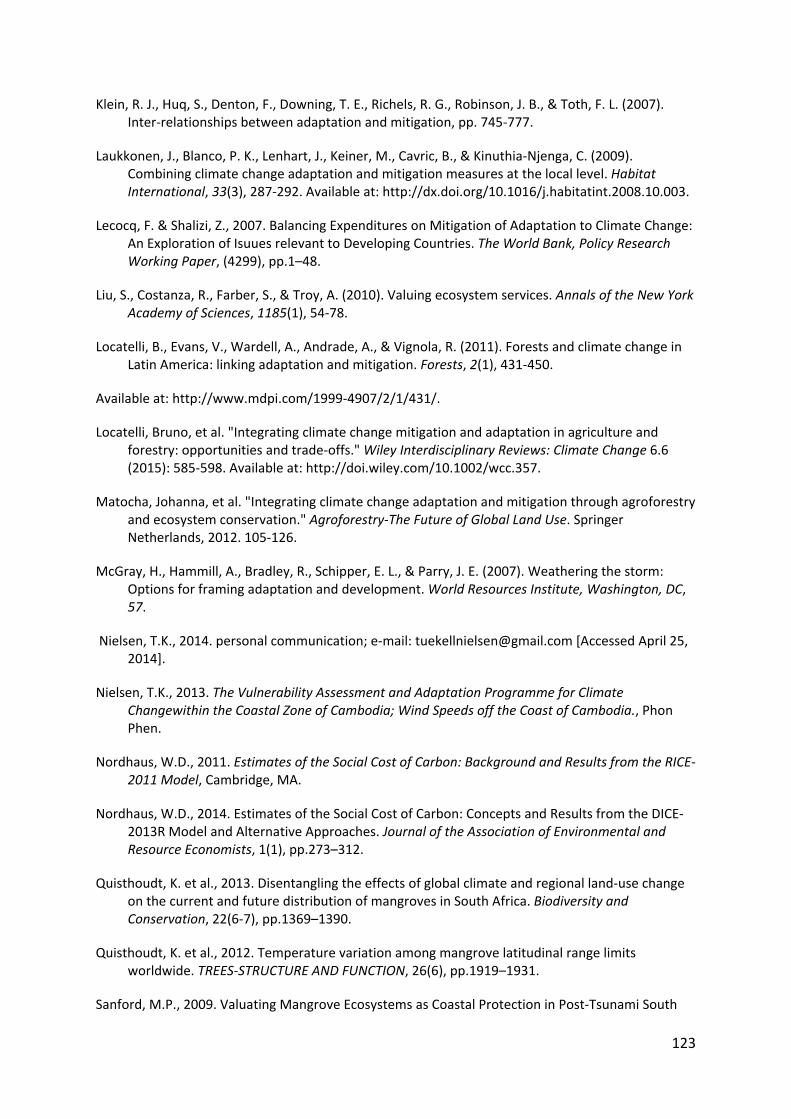
123  

Klein, R. J., Huq, S., Denton, F., Downing, T. E., Richels, R. G., Robinson, J. B., & Toth, F. L. (2007). Inter‐relationships between adaptation and mitigation, pp. 745‐777. 

Laukkonen, J., Blanco, P. K., Lenhart, J., Keiner, M., Cavric, B., & Kinuthia‐Njenga, C. (2009). Combining climate change adaptation and mitigation measures at the local level. Habitat International, 33(3), 287‐292. Available at: http://dx.doi.org/10.1016/j.habitatint.2008.10.003. 

Lecocq, F. & Shalizi, Z., 2007. Balancing Expenditures on Mitigation of Adaptation to Climate Change: An Exploration of Isuues relevant to Developing Countries. The World Bank, Policy Research Working Paper, (4299), pp.1–48.   

Liu, S., Costanza, R., Farber, S., & Troy, A. (2010). Valuing ecosystem services. Annals of the New York Academy of Sciences, 1185(1), 54‐78. 

Locatelli, B., Evans, V., Wardell, A., Andrade, A., & Vignola, R. (2011). Forests and climate change in Latin America: linking adaptation and mitigation. Forests, 2(1), 431‐450. 

Available at: http://www.mdpi.com/1999‐4907/2/1/431/. 

Locatelli, Bruno, et al. "Integrating climate change mitigation and adaptation in agriculture and forestry: opportunities and trade‐offs." Wiley Interdisciplinary Reviews: Climate Change 6.6 (2015): 585‐598. Available at: http://doi.wiley.com/10.1002/wcc.357. 

Matocha, Johanna, et al. "Integrating climate change adaptation and mitigation through agroforestry and ecosystem conservation." Agroforestry‐The Future of Global Land Use. Springer Netherlands, 2012. 105‐126. 

McGray, H., Hammill, A., Bradley, R., Schipper, E. L., & Parry, J. E. (2007). Weathering the storm: Options for framing adaptation and development. World Resources Institute, Washington, DC, 57. 

 Nielsen, T.K., 2014. personal communication; e‐mail: tuekellnielsen@gmail.com [Accessed April 25, 2014]. 

Nielsen, T.K., 2013. The Vulnerability Assessment and Adaptation Programme for Climate Changewithin the Coastal Zone of Cambodia; Wind Speeds off the Coast of Cambodia., Phon Phen. 

Nordhaus, W.D., 2011. Estimates of the Social Cost of Carbon: Background and Results from the RICE‐2011 Model, Cambridge, MA. 

Nordhaus, W.D., 2014. Estimates of the Social Cost of Carbon: Concepts and Results from the DICE‐2013R Model and Alternative Approaches. Journal of the Association of Environmental and Resource Economists, 1(1), pp.273–312. 

Quisthoudt, K. et al., 2013. Disentangling the effects of global climate and regional land‐use change on the current and future distribution of mangroves in South Africa. Biodiversity and Conservation, 22(6‐7), pp.1369–1390. 

Quisthoudt, K. et al., 2012. Temperature variation among mangrove latitudinal range limits worldwide. TREES‐STRUCTURE AND FUNCTION, 26(6), pp.1919–1931.  

Sanford, M.P., 2009. Valuating Mangrove Ecosystems as Coastal Protection in Post‐Tsunami South 

124  

Asia. Natural Areas Journal, 29(1), pp.91–95. 

Sauer, J. & Wossink, A., 2013. Marketed outputs and non‐marketed ecosystem services: the evaluation of marginal costs. EUROPEAN REVIEW OF AGRICULTURAL ECONOMICS, 40(4), pp.573–603.  

Stern, N., 2007. The Economics of Climate change: the Stern review, Cambridge University press. 

Tol, R.S.J., 2013. Targets for global climate policy: An overview. Journal of Economic Dynamics and Control, 37(5), pp.911–928. Available at: http://linkinghub.elsevier.com/retrieve/pii/S0165188913000092. 

Tol, R.S.J., 2008. The Social Cost of Carbon: Trends, Outliers and Catastrophes. Economics The Open‐Access, Open‐Assessment E‐journals, 2(25), pp.1–24.  

Tomlinson, P.B., 1986. The Botany of Mangroves P. S. Ashton et al., eds., Cambridge University Press. 

VAAP LDCF, 2013. Commune project proposal 2013; Mangrove Restoration, Peam Krasaob, Cambodia. 

Verchot, L.V. et al., 2007. Climate change: linking adaptation and mitigation through agroforestry. Mitigation and Adaptation Strategies for Global Change, 12(5), pp.901–918.  

Warren, R. et al., 2012. Scoping Study: Modelling the interaction between mitigation and adaptation for decision making, Available at: http://www.nature.com/doifinder/10.1038/nature08823. 

Watkiss, P.,  Benzie,M. and Klein, R.T.J., "The complementarity and comparability of climate change adaptation and mitigation." Wiley Interdisciplinary Reviews: Climate Change 6.6 (2015): 541‐557. 

 XE, 2014. XE Currency Table : USD ‐ US Dollar. Available at: http://www.xe.com/currencytables/?from=USD&date=2014‐02‐10 [Accessed October 2, 2014]. 

 

   

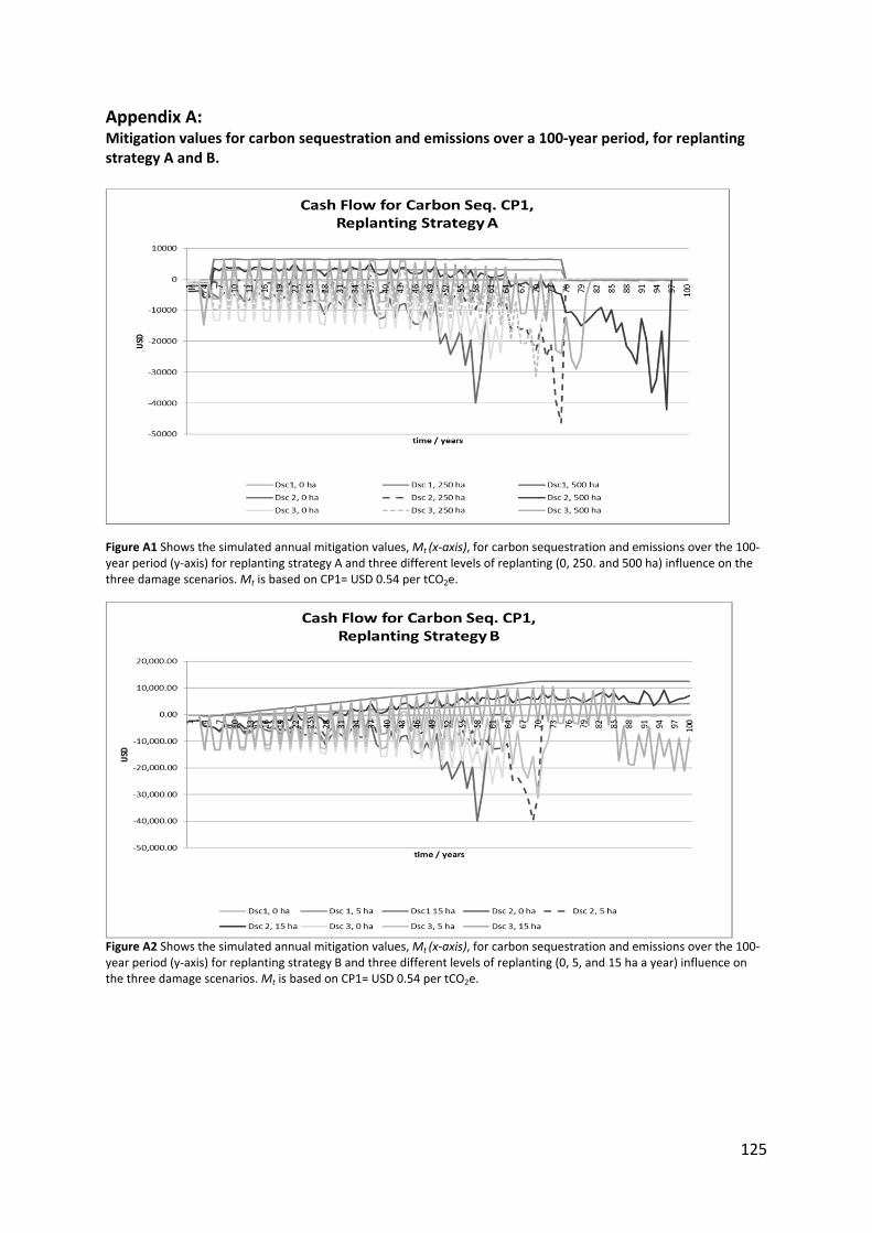
125  

Appendix A: Mitigation values for carbon sequestration and emissions over a 100‐year period, for replanting strategy A and B.  

 

Figure A1 Shows the simulated annual mitigation values, Mt (x‐axis), for carbon sequestration and emissions over the 100‐year period (y‐axis) for replanting strategy A and three different levels of replanting (0, 250. and 500 ha) influence on the three damage scenarios. Mt is based on CP1= USD 0.54 per tCO2e.  

 Figure A2 Shows the simulated annual mitigation values, Mt (x‐axis), for carbon sequestration and emissions over the 100‐year period (y‐axis) for replanting strategy B and three different levels of replanting (0, 5, and 15 ha a year) influence on the three damage scenarios. Mt is based on CP1= USD 0.54 per tCO2e. 

   

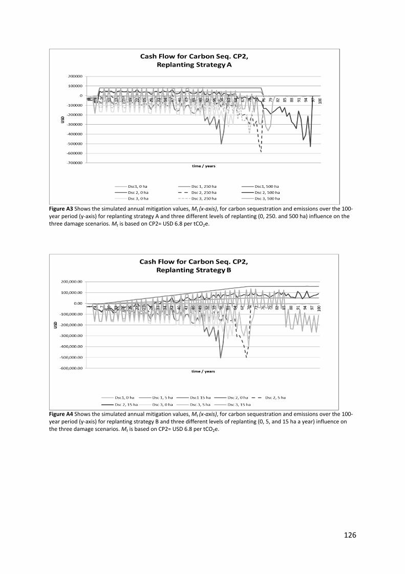
126  

 Figure A3 Shows the simulated annual mitigation values, Mt (x‐axis), for carbon sequestration and emissions over the 100‐year period (y‐axis) for replanting strategy A and three different levels of replanting (0, 250. and 500 ha) influence on the three damage scenarios. Mt is based on CP2= USD 6.8 per tCO2e.  

  

 Figure A4 Shows the simulated annual mitigation values, Mt (x‐axis), for carbon sequestration and emissions over the 100‐year period (y‐axis) for replanting strategy B and three different levels of replanting (0, 5, and 15 ha a year) influence on the three damage scenarios. Mt is based on CP2= USD 6.8 per tCO2e. 

  

127  

 

Figure A5 Shows the simulated annual mitigation values, Mt (x‐axis), for carbon sequestration and emissions over the 100‐year period (y‐axis) for replanting strategy A and three different levels of replanting (0, 250. and 500 ha) influence on the three damage scenarios.  Mt is based on CP3= USD 13.18 per tCO2e.  

  

 Figure A6  Shows the simulated annual mitigation values, Mt (x‐axis), for carbon sequestration and emissions over the 100‐year period (y‐axis) for replanting strategy B and three different levels of replanting (0, 5, and 15 ha a year) influence on the three damage scenarios. Mt is based on CP3= USD 13.18 per tCO2e. 

    

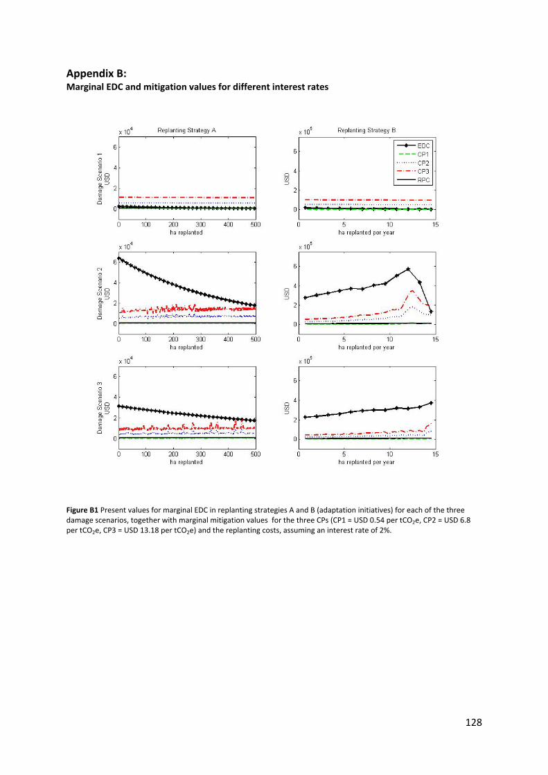
128  

Appendix B: Marginal EDC and mitigation values for different interest rates  

 Figure B1 Present values for marginal EDC in replanting strategies A and B (adaptation initiatives) for each of the three damage scenarios, together with marginal mitigation values  for the three CPs (CP1 = USD 0.54 per tCO2e, CP2 = USD 6.8 per tCO2e, CP3 = USD 13.18 per tCO2e) and the replanting costs, assuming an interest rate of 2%. 

129  

 

 Figure B2 Present values for marginal EDC in replanting strategies A and B (adaptation initiatives) for each of the three damage scenarios, together with marginal mitigation values  for the three CPs (CP1 = USD 0.54 per tCO2e, CP2 = USD 6.8 per tCO2e, CP3 = USD 13.18 per tCO2e) at an interest rate of 20%. 

     

130  

Appendix C: Not part of submitted paper  Marginal EDC, extreme carbon prices and mitigation values for 4% and 12% interest rates  

 Figure C1 The marginal avoided EDC for the two replanting strategies A and B (adaptation initiatives) in each of the three damage scenarios (the black solid lines with dots) together with marginal mitigation values for the three CPs CP1 = USD 50 per tCO2e, CP2 = USD 100 per tCO2e, CP3 = USD 200 per tCO2e (the dashed lines). The thin black line shows the marginal replanting costs. All assume a discount rate of four per cent. 

 

131  

 Figure C2 The marginal avoided EDC for the two replanting strategies A and B (adaptation initiatives) in each of the three damage scenarios (the black solid lines with dots) together with marginal mitigation values for the three CPs CP1 = USD 50 per tCO2e, CP2 = USD 100 per tCO2e, CP3 = USD 200 per tCO2e (the dashed lines). The thin black line shows the marginal replanting costs. All assume a discount rate of 12 per cent. 

 

132

Paper 3 

 

Empirically Based Analysis of Households Coping with Unexpected Shocks in the Central Himalayas   

Lea Ravnkilde Møller1*, Carsten Smith‐Hall2, Henrik Meilby2, Santosh Rayamajhi3, Lise Byskov 

Herslund4, Helle Overgaard Larsen2, Øystein Juul Nielsen5, Anja Byg6 

 

1 UNEP DTU Partnership, DTU Management Engineering, Technical University of Denmark, 

Marmorvej 51, DK‐2100 Copenhagen, Denmark  

2 Department of Food and Resource Economics, University of Copenhagen, Rolighedsvej 25, 

1958 Frederiksberg C, Denmark 

3 Institute of Forestry, Tribhuvan University, 33700 Pokhara, Nepal 

4 Department of Geosciences and Natural Resource Management, University of 

Copenhagen, Rolighedsvej 23, 1958 Frederiksberg C, Denmark 

5 International Woodland Company, Amalievej 20, 1875 Frederiksberg C, Denmark 

6Social, Economic and Geographical Sciences Group, The James Hutton Institute, 

Craigiebuckler, Aberdeen AB15 8QH, Scotland, UK 

 

Manuscript to be submitted, to Regional Environmental Change.  

 

Key words: Coping, livelihoods, vulnerability, Nepal 

 

Abstract Climate  change may  significantly  impact  the  large number of households  in developing  countries depending on agricultural production, not least through changes in the frequency and/or magnitude of  climatic  hazards  resulting  in  household  income  shocks.  This  paper  analyses  rural  households’ responses to past experience of and future expectations to substantial and unexpected negative and positive agricultural  income shocks. Empirical data  is derived  from an environmentally‐augmented structured  household  (n=112)  survey  in  the  high mountains  of  central  Nepal. Multinomial  logit regression, using data on rural household demographics, assets (agricultural land, livestock), value of other assets such as  furniture, bicycles, and agricultural  implements), and  income sources showed that household  coping  choices  are determined by opportunities  to  generate  cash. We  argue  that 

133

public  policies  should  enhance  the  ability  of  rural  household  to  generate  cash  income,  including through environmental products. 

 

Introduction 

Evidence of climate change  is beginning to show. Developing countries are especially vulnerable to 

climate change due  to a combination of substantial projected biophysical changes, strong  reliance 

on climate‐sensitive sectors such as agriculture, and widespread poverty (Adger et al. 2003, Dodman 

et  al.  2009,  Hijioken  et  al.  2014,  Huq  and  Reid  2004).  However,  even  without  climate  change, 

households engaged  in agriculture experience weather related shocks – e.g. from draughts, floods, 

frost and hail storms,  irregular snow, pest and diseases –  resulting  in production  losses  leading  to 

lower total household income and possibly an increase in expenditures, e.g. to purchase new seeds. 

While rural households often have established strategies for coping with known challenges (Dodman 

et al. 2009) climate change is expected to represent additional challenges in the form of new climatic 

phenomena and/or changes in the frequency or magnitude of existing climatic hazards (Hijioka et al. 

2014). 

Coping constitutes the use of available skills, resources, and opportunities to address, manage, and 

overcome adverse conditions, with  the aim of achieving basic  functioning  in  the  short  to medium 

term; while coping capacity is the ability of people, organizations, and systems, again using available 

skills,  resources,  and  opportunities,  to  address, manage,  and  overcome  adverse  conditions  (IPCC 

2012).  A  defining  feature  of  coping  is  the  focus  on  the  short  to  medium  term  in  contrast  to 

adaptation, which  refers  to  longer  term  responses.   The  two  concepts  are, however,  related  and 

Smit and Wandel  (2006) define adaptation as  the expansion of coping ranges. On  the other hand, 

short‐term coping strategies can also undermine or prevent longer‐term adaptation and reduce the 

coping  range,  for  example where  shock  responses,  such  as  the  sale  of  productive  assets,  leave 

households more vulnerable to future shocks (e.g. Smit and Wandel 2006). Coping may be proactive, 

e.g. when households reduce risk by diversifying  income generating activities, avoid profitable but 

potentially hazardous actions, or pool risk through social and  institutional networks (Wunder et al. 

2014).  Reactive  coping  responses  depend  on  the  size  of  the  shock  and  include  actions  such  as 

income and consumption smoothing, assets sales, resource reallocation (e.g. finding work off‐farm, 

increasing labour time, taking children out of school that can contribute more labour) (Wunder et al. 

2014). Household coping responses and choices of coping strategies are shaped by  their access  to 

resources and  liberty of actions (Eriksen 2005, Sen 2003). Household resources can be divided  into 

134

human,  natural,  financial,  social,  and  physical  capitals  according  to  the  sustainable  livelihood 

framework (e.g. DFID 1999). Liberty of actions is inter alia influenced by households’ priorities, past 

experiences, expectations for the future, and social and cultural norms limiting which responses are 

considered  possible,  appropriate,  and  acceptable  (e.g.,  Adger  et  al.  2009,  Coulthard  2008,  2012, 

Nielsen and Reenberg 2010).  

In this paper, we analyse rural households’ coping responses in relation to unexpected negative and 

positive shocks to their income from agricultural production in the high mountains of central Nepal, 

and  relate  their  responses  to  household  resources.  We  define  negative  shocks  as  substantial 

unexpected shortage from agricultural production, e.g. due to drought, too much rain, landslides, or 

irregular  snowfall,  causing  an  income  loss.  Positive  shocks  are  defined  as  an  unexpected  large 

income  from agricultural production as compared  to a normal year. Rural households  in  the study 

area  generally  have  limited  economic  resources,  low  levels  of  technology,  low  skill  levels,  poor 

infrastructure,  and  weak  institutions  (Rayamajhi  et  al.  2012)  –  factors  which  are  expected  to 

contribute to high  levels of vulnerability (Wunder et al. 2014). Their  liberty of actions (Sen 2003)  is 

arguably limited by the low asset levels and macro‐level constraints, including political instability and 

low  levels of economic growth, even  if new opportunities also emerge, such as  through migration 

(Walelign et al. 2016).     

We answer the two questions: 

1. Which coping responses have rural households utilised  in the past to overcome unexpected 

shocks, and which coping responses do they expect to use in the future? 

2. How  do  households  differ  in  their  responses  and  how  is  this  linked  to  their  livelihood 

strategies and assets? 

We hypothesise that: 1. Households choose coping responses that are complementary, and 2. 

Households’ coping responses are shaped by their assets and livelihood strategies. 

 

Methods 

 Study Area 

The Lete and Kunjo Village Development Committees (VDCs – the smallest local administrative unit 

in Nepal) lie in the lower part of Mustang District (28°34'‐28°41' N and 83°33'‐83°44' E) in the 

Western Development Region of Nepal. The villages are located at an altitude of above 2,000 metres 

135

in a temperate to sub‐alpine climate with occasional windstorms, hail, and snow. The annual 

average precipitation was 1242 millimetres and the yearly average temperature was 11.7°C (in 2006, 

unpublished data from Dept. of Hydrology and Meteorology). The study area is situated within the 

Annapurna Conservation Area (ACA), world famous for trekking tourism, and was recently connected 

to an all‐weather road (Baral et al. 2007, Larsen et al. 2014). Land use is characterised by upper and 

higher elevation subsistence production type systems (Metz 1989, 1990, Olsen 1996): large areas of 

rain‐fed fields, whose fertility is maintained through use of composted manure. Average per 

household land holding was 1.1 ha and the main crops are maize, barley, buckwheat, potato, and 

beans. Average livestock holding was 8.7 Tropical Livestock Units (TLU) dominated by cattle, sheep, 

and goats. About 5,017 ha are covered with forest, including natural forests, plantations, and shrubs; 

a similar area of grassland under community‐based management was available (Larsen et al. 2014). 

Forests are dominated by Pinus wallichiana and some old‐growth Tsuga dumosa, two valuable 

timber species. The main forest products are grass, bamboo, firewood, pine needle, and timber and 

can be collected or purchased on the basis of rules and restrictions made by the forest user groups 

(FUGs); only minor extraction of timber was permitted (Larsen et al. 2014).  

The  study  area  is  characterised  by  low  income  levels  and widespread  poverty, with  ca.  13 %  of 

average total household income derived from crops, 16 % from livestock, 26 % from environmental 

sources, and 42 %  from non‐farm activities, e.g.  remittances and gifts, self‐owned businesses, off‐

farm wage  labour, or government pensions  (Rayamajhi et al. 2012). Environmental  income plays a 

main  role,  especially  for  poor  households, who  collect  non‐timber  forest  products  for  sale while 

better off households  rely on non‐farm  income  (Rayamajhi et al. 2012). Recent  research  from  the 

study  area  (Walelign  et  al.  2016)  indicates  that  a  common  pathway  out  of  poverty  is  household 

accumulation of assets through farming, petty trading, and migratory work. Environmental  income 

has also been shown to reduce  income  inequality (Chhetri et al. 2015) while establishment of road 

infrastructure increased household incomes and decreased income inequality (Charlery et al. 2016).  

 Climate Change in Nepal 

The  few  existing  studies  of meteorological  records  for  Nepal  show  an  increase  in  annual mean 

temperature  over  the  past  30‐50  years,  with  higher  increases  at  higher  elevations  (Khan  2005, 

Marahatta 2009, McSweeney 2008, Shrestha et al. 1999). Analyses of precipitation patterns over the 

past 50 years show mixed results (Ichiyanagi et al. 2007, Kansakar et al. 2004, Khan 2005, Marahatta 

2009, McSweeney 2008,  Shrestha  et  al. 2000).  The  average  temperature  is predicted  to  increase 

from 1.3 to 4.3 C by the middle of the 21st century with the mountainous north experiencing the 

136

highest increase. With regard to precipitation, models tend to predict a summer monsoon increase 

and a winter precipitation decrease  (Khan 2005, McSweeney 2008).  Importantly,  the  likelihood of 

‘heavy  rainfall’ events  is also predicted  to  increase. Future climate change  risks  in  the  study area, 

while uncertain and difficult  to quantify, are  thus  increases  in extreme event  frequency and  intra‐

annual rainfall variability. The latter may not be as dramatic as the former, but can make it difficult 

for farmers to plan activities such as sowing and harvesting or what to plant.  

 

Data Collection 

Data  was  collected  using  two  survey  instruments,  both  administered  in  2009.  The  first  was  a 

structured  household  (n=186)  survey  using  the  Poverty  Environment  Network  (PEN)  protocol 

(Angelsen et al. 2011, Larsen et al. 2014) including annual surveys (at survey start and end) and four 

quarterly income surveys. The data collection period spanned a complete year from December 2008 

to November 2009. The annual surveys  registered asset data while  the quarterly surveys  included 

recording of all environmental, farm, and non‐farm incomes. Allocation of own labour into different 

activities  is difficult to disaggregate – a common phenomenon  in the development  literature – and 

was not  subtracted  from net  incomes  (Nielsen et al. 2013, Rayamajhi et al. 2012).  In most  cases, 

market prices were used to calculate income values; in cases with thin or missing markets, standard 

methods  for  estimating  subsistence  product  values  were  applied  (Rayamajhi  and  Olsen  2009, 

Wunder et al. 2011).  

The second  instrument was administered, alongside  the survey end annual questionnaire,  to elicit 

household‐level  responses  to  substantial unexpected  shocks  (negative or positive)  in  the past  five 

years as well as  their expected  coping  responses  to a hypothetical  shock  in  the  coming year  (the 

instrument  is  provided  in  Appendix  1).  A  number  of  households were  excluded  as  they  did  not 

complete  all  the  income  surveys  or  could  not  be  located  at  the  time  of  interview;  the  survey 

included 112 households. Specifically, for the past five years, the survey recorded shocks and their 

impact on crop production (loss or gain) compared to the expected normal value for each year; we 

distinguished moderate  shocks  (< 50 %  loss or gain) and  substantial  shocks  (> 50 %), and used a 

discrete  range  (0‐20  %,  21‐80  %  or  81‐100  %)  to  measure  the  importance  of  responses,  each 

counting  as  an  observation.  A  similar  approach  was  used  to  elicit  responses  to  hypothetical 

situations taking place next year. This produced 663 and 501 observations  for  loss and gain  in the 

past, and 795 and 787 observations for next year responses.   

 

   

137

Data Analysis 

To enable comparison between households, including the different predicted variables’ influence on 

households’ choices of coping  responses, we accounted  for household size and possible effects of 

economics  of  scale  by  reporting  all  monetary  values  per  adult  equivalent  unit  (AEU)  following 

common practice  (Cavendish 2002). The percentage of  income  loss or gain was calculated on  the 

basis of the value that was obtained as the normal income value. The households’ total income per 

AEU was calculated by summarising all net  income types per household. Based on Rayamajhi et al. 

(2012),  it  is  assumed  that  income  level  and  quartile membership  have  a  significant  influence  on 

choice of coping responses.  

We applied multinomial logit (MNL) regression to analyse households’ past behaviour and expected 

future  behaviour  in  response  to  unexpected  positive  and  negative  shocks  to  agricultural  income. 

Following  the argumentation  in Gebrehiwot and van der Veen  (2013),  the multinomial adaptation 

model is the correct choice when there are more than two alternatives. We assume that households’ 

responses  are  rational  and  that  they will  choose  the  coping  response  that maximises  their utility 

(McFadden  1973).  This makes  it  possible  to  identify  determinants  of  the  households’  choice  of 

coping responses through discrete choice modelling. Assume that farmer  i aims to maximise utility 

through his choice of coping response j (j = 1, 2,… j). He will choose coping response j rather than k, if 

the  perceived  benefit  of  j  is  larger  than  for  k.  The  relative  probability  of  the  coping  response 

variables is given by the log odds ratio (Eq. 1) (Green 2003): 

 

     (1) 

 

where xi is a vector of household characteristics and βj are the corresponding coefficients. The most 

preferred coping response is used as the base category for normalization, k. These coping responses 

are  used  as  reference  groups  as  they  are  assumed  available  to  all  households  regardless  of 

characteristics and status, e.g.  income,  land ownership, or debt. Reduced consumption and saving 

cash are used as references in the MNL regressions for loss and gain in income, respectively. 

 

We account for clusters among the households by allowing for  intragroup correlation, relaxing the 

requirement  that  the  observations  must  be  independent.  We  assume  that  observations  are 

independent  across  households,  but  not  within  households,  as  our  data  contain  repeated 

information on households’ past and expected  future behaviour  in  relation  to  income  loss or gain 

from unexpected shocks. 

138

 

 The  individual explanatory variables were tested using a Type  III (Wald chi2) test. MNL regressions 

were carried out using the statistical software, StataIC 11. 

 

Results 

 Household Income and Asset Data 

The overview of household  income and asset values (Table 1) documents widespread poverty, e.g. 

the average total income is 1.6 USD/AEU/day (below the global poverty line of 1.9 USD/capita/day), 

ranging from 0.5 – 3.5 across the quartiles. Agricultural land is limited as is the number of livestock. 

The best‐off quartile households own the most land; 9.9 % of households do not own any land and 

mainly belong  to  the  ‘Poorest’  income quartile.  Environmental  income  and wage  income  are  the 

most  important  to  the  two  poorer  quartiles,  while  business  income  and  remittances  are more 

dominant  for  higher  income  households.  When  it  comes  to  the  size  and  composition  of  the 

households  – male,  female,  children,  elderly  –  households  in most  well‐off  quartile  tend  to  be 

smaller  than  in  the other  three quartiles. Furthermore,  literacy  is high  (83 %) and  the mean adult 

educational level is 6.6 years of schooling (Rayamajhi et al. 2012).    

 

Households’ Coping Responses 

The questionnaire on coping with unexpected loss or gain included 12 coping response options. To 

use the data in the MNL regressions, the response variables were aggregated in seven and eight 

groups, for loss and gain respectively, as specified in Tables 2‐5 that also present the sequence of 

households’ chosen coping responses. 

Table 2 presents an overview of household coping responses to shocks reducing agricultural income. 

The most  common  first  coping  choice  is  to  reduce household  consumption  (A, 37%),  followed by 

obtaining  loans or assistance (B, 38%) and spending savings (C, 51%). The most common responses 

are consumption reduction (done by 32% of households), spend savings (27%), and obtaining loans 

and assistance (21%).  

139

Table 1 Household absolute mean asset and income across income quartiles. Net income figures in parentheses are share of annual total household income.  

  Poorest  Poor  Medium  Less poor  Sample mean (SD)  Min.‐max. range 

  Lowest 25%  25‐50%  50‐75%  top 25%  n=112 

Description  Units  n=28  n=28  n=28  n=28 

Household size   AEU  4.2  4.2  3.8  3.5  3.9 (1.1)  1‐8 

No. of adult females in HH    1.7  2.0  1.5  1.7  1.7 (1.0)  0‐5 

No. of adult males in HH    2.2  2.1  1.9  1.2  1.8 (1.2)  0‐5 

No. of children in HH    1.4  1.1  1.0  0.7  1.1 (1.1)  0‐4 

No. of elderly in HH    0.5  0.5  0.5  0.9  0.6  (0.8)  0‐2 

Farmland owned   Ha  0.7  0.9  1.2  1.5  1.1 (0.8)  0‐3.4 

Livestock  TLU per AEU   

0.5  0.8  1.5  2.9  1.4 (2.6)  0‐18.2 

Net environmental income   USD per AEU  48.5 (24.6%)  74.8 (21.5%)  79.1 (14.8%)  132.3 (10.2%)  83.7 (95.3) (14%)  ‐237.6‐648.7 

Income: land rented out   USD per AEU  0.7 (0.3%)  2.0 (0.6%)  5.1 (0.9%)  12.8 (1.0%)  5.2 (22.1) (0.9%)  0‐219.4 

Net income from livestock  USD per AEU  63.8 (32.5%)  107.9 (31.0%)  137.5 (25.7%)  560.6 (43.3%)  217.5 (627.1) (36.6)  ‐107.3 

Net income from crops  USD per AEU  21.8 (11.1%)  56.6 (16.3%)  78.8 (14.7%)  126.5 (9.8%)  70.9 (87.3) (12%)  ‐16.6 

Net business income   USD per AEU  14.1 (7.2%)  27.7 (8.0%)  157.6 (29.5%)  301.5 (23.3%)  125.2 (233.9) (21.1%)  ‐30.4‐1304.2 

Net wage income   USD per AEU  24.6 (12.5%)  38.3 (11.0%)  21.7 (4.1%)  20.9 (1.6%)  26.4 (45.6) (4.4%)  0‐225.5 

Pension, support from NGO 

or government  USD per AEU  4.4 (2.2%)  11.1 (3.2%)  7.9 (1.5%)  3.4 (0.3%)  6.7 (23.5) (1.1%)  0‐148.3 

Remittance   USD per AEU  18.8 (9.5%)  29.4 (8.5%)  46.9 (8.8%)  136.8 (10.6%)  58.0 (136) (9.8%)  0‐767.8 

No remittanceA 

0‐1  0.8  0.7  0.7  0.7  0.7 (0.4)  0‐1 

Net Total Income   USD per AEU  196.7 (100%)  347.8 (100%)  534.4 (100%)  1,294.9 (100%)  593.5 (736.6) (100%)  79.4‐7,032 

Savings in bank and jewellery  USD per AEU  346.0  314.9  585.6  1,775.7  755.6 (1,481.9)  0‐12,348.4 

Value of all assets  USD per AEU  1,496.5  1,537.8  3,025.4  5,786.9  2,961.7 (3,846.2)  ‐569.5‐24,815 

Cost of power for irrigation   USD per AEU  3.0  1.5  0.9  3.3  2.2 (5.3)  0‐45.3 

Debt   USD per AEU  179.7  290.5  410.1  384.1  316.1 (361)  0‐1,695 

Total expenditure   USD per AEU  337.0  344.6  477.1  711.7  467.6 (300)  144.2‐1,703 

A Dummy variable takes the value of 1 if the household does not receive remittance and 0 otherwise. 

140

 

Table 2 Rural households’ coping responses, over the past five years, following a substantial unexpected negative shock resulting in an agricultural income loss. 

No.  Response variables  A  B  C  Total  Description 

1  Spend savings  17%  11%  51%  27%  The HH spends savings and sells non‐agricultural assets. 

2  Remittance  3%  4%  2%  3% The HH decides that a member will work outside the community to generate remittance. 

3 Reduce consumption 

37%  29%  29%  32%  The HH reduces consumption. 

4  Loan or assistance  21%  38%  6%  21% The HH takes a loan from a money lender or bank or get assistance from NGO or others. 

5 Sell livestock or land 

7%  5%  3%  5%  The HH chooses to sell livestock or land. 

6  Work more  15%  13%  9%  12% The HH does extra casual work, or harvests, uses or sells more environmental products. 

  Total  100%  100%  100%  100%   

 

Household first choice in response to shocks increasing agricultural incomes (Table 3) is to increase 

consumption (A, 39%) followed by  loan repayment (B, 32%) and saving up cash (C, 61%). The most 

common  responses  are  to  save  cash  (done  by  31%  of  households)  followed  by  loan  repayment 

(25%), and increased consumption (24%). Other responses are not frequent.  

 

Table 3 Rural households’ coping responses, over the past five years, following a substantial unexpected positive shock resulting in an agricultural income gain. 

No.  Response variables  A  B  C  Total  Description 

1  Save cash  14%  14%  61%  31%  The HH saves cash. 

2  Remittance stop  1%  15%  1%  5% HH members stop sending remittances or return to the HH. 

3  Increase consumption  39%  24%  11%  24% The HH increases consumption and purchases goods. 

4  Pay loan back  32%  32%  11%  25% The HH pays back loans to money lender or bank, or sends gifts to others. 

5  Purchase agricultural assets  5%  4%  3%  4%  The HH invests in land and livestock. 

6  Reduce income activities  3%  3%  10%  5% The HH stops doing extra casual work or limits the extent of collecting, using or selling environmental products. 

7  Purchase other goods  7%  7%  4%  6% The HH chooses to purchase or invest in other goods. 

  Total  100%  100%  100%  100%   

 

Asked about their responses to a negative shock reducing income next year, households expected to 

reduce  consumption  (the  dominant  first  and  second  choice:  A,  30%  and  B,  30%)  followed  by 

spending  of  savings  (C,  40%)  (Table  4).  The  three  most  common  responses  are  consumption 

141

reduction (27% of all households), savings spending (23%), and obtaining loans or assistance (23%). 

This response pattern is similar to that for past behaviour (Table 2); however, there seems to be an 

increased interest in pursuing remittances as a coping response (7% vs. 3%). 

 

Table 4 Rural households’ anticipated choices of coping responses in reply to an imagined substantial unexpected negative shock in the coming year resulting in an agricultural income loss. 

No. Response variables 

A  B  C  Total  Description 

1  Spend savings  14%  13%  40%  23% The HH spends savings and sells other non‐agricultural assets. 

2  Remittance  11%  9%  2%  7% The HH decides that a member will work outside the community to send remittance. 

3 Reduce consumption 

30%  30%  20%  27%  The HH reduces consumption. 

4  Loan or assistance  25%  25%  20%  23% The HH chooses to take a loan from a money lender or bank or get assistance from NGO or others. 

5 Sell livestock or land 

7%  8%  8%  8%  The HH chooses to sell livestock or land. 

6  Work more  13%  15%  9%  12% The HH does extra casual work, or harvests, uses or sells more environmental products. 

  Total  100%  100%  100%  100%   

 

Table 5 shows the expected household responses to a positive shock resulting in an income gain. The 

most common first and second response choices are to  increase consumption (A, 25% and B, 26%) 

followed by saving cash (C, 32%). The most common responses are loan repayment (done by 24% of 

households) followed by increased consumption (22%) and cash saving (20%). Again, this is similar to 

the  past  response  pattern  (Table  3)  though  expected  responses  seem  more  evenly  distributed 

compared to past actual behaviour.  

 

   

142

Table 5 Rural households’ anticipated coping responses in reply to a substantial unexpected positive shock in the coming year resulting in an agricultural income gain. No.  Response variables  A  B C Total Description

1  Save cash  15%  11% 32% 20% The HH saves cash. 

2  Remittance stop  9%  3%  1%  4%  HH members stop sending remittance or return to the HH. 

3  Increase consumption  25%  26%  15%  22%  The HH  increases  consumption  and  purchases goods. 

4  Pay loan back  19%  23%  28%  24%  The  HH  pays  back  loan  to  money  lender  or bank, or sends gifts to others. 

5  Purchase agricultural assets  15%  16%  14%  15%  The HH chooses to invest in land and livestock. 

6  Reduce income activities  9%  12%  4%  9% The HH stops doing extra casual work or  limits the  extent  of  collecting,  using  or  selling environmental products

7  Purchase other goods  8%  8%  5%  7%  The HH chooses  to purchase or  invest  in other goods. 

  Total  100%  100% 100% 100%

 

Results of the MNL Regressions 

In  the MLN  regressions,  the  coefficients  reflect  the  effects  of  the  explanatory  variables  on  the 

likelihood of  the households  choosing  a  coping  response  relative  to  the  coping  response used  as 

reference. Each of the explanatory variables were tested against the response variables  in a minor 

MNL regression (not presented) to determine if they independently influenced households’ choice of 

coping response. If the probability of the chi2 test (P > chi2 < 0.10) for the MNL regression was equal 

to or below  10%,  the  explanatory  variable was  included. As  each  individual  household  answered 

questions with  several  answers, we  estimate  each of  the presented MNL  regression models  as  a 

cluster model with the household being the cluster. The Type III test was used to test each individual 

explanatory variable. Explanatory variables significant at the 10% level were included in the relevant 

final  model.  A  total  of  14  explanatory  variables  were  significant  to  the  households’  past  and 

expected  future choices of coping responses  in case of agricultural  income  loss or gain. Tables 6‐9 

show  the  significant  explanatory  variables  for  each of  the  four MNL  regressions;  the  explanatory 

variables are listed in the same order and left blank  if not relevant. Appendix 2  presents all results 

for the four MNL regressions (i.e. also insignificant explanatory variables).  

133

Table 6 MLN regression results for coping responses to past situations with an unexpected agricultural income loss 

   Coping responses 1 Spend savings   

2 Obtain remittance   

4 Loan or assistance   

5 Sell livestock or land   

6 Work more   

chi2 test  

Coef.   z  Coef.   z  Coef.   z  Coef.   z  Coef.   z  P > chi2 

No.  Explanatory variables             

1  Household size (AEU)  0.147  1.45  0.529  1.92*  ‐0.112  0.79  0.149  0.58  ‐0.0987  0.35  0.0788* 

2 No. of adult males in HH (AEU) 

‐0.337  3.2***  ‐0.0865  0.37  ‐0.229  1.68*  ‐0.117  0.47  ‐0.0493  0.27  0.0453** 

3  Farmland owned (ha)                                  

4  Livestock(TLU/AEU)             

5 

Net income from environmental products (USD/aeu)  

                                

6 Income from land rented out  

                    

7 Income quartile: ‘Less 

poor’ (4)A 

                                

8 Net business income (USD/AEU) 

                    

9 Pension, support from NGO or government (USD/AEU)  

‐0.007517  3.95***  0.0068381  0.58  ‐0.0189  3.06**  ‐0.009  0.56  ‐0.0018  0.28  0*** 

10  Remittance (USD/AEU)   ‐0.00135  2.44**  0.001958  2.02**  0.000  0.58  ‐0.005  1.97**  ‐0.0048  2.33**  0*** 

11 Value of all assets (USD/AEU)  

‐0.00004  2.08**  ‐0.000104  1.27  0.000  3.84***  0.000  1.06  ‐0.0004  3.83***  0.0002*** 

12 Cost of power for irrigation (USD/AEU)  

‐0.003424  0.41  ‐0.050797  0.77  ‐0.0550  2.29**  ‐0.271  1.91*  0.0088  0.34  0.0214** 

13  Debt (USD/AEU)                

14  Size of shock B                                  

Constant  0.1295677  0.41  ‐4.234237  3.88***  1.074  2.27**  ‐1.467  1.59  0.4951  0.48 

  Number of obs. = 663, Pseudo R2 = 0.0504 

* p<0.1, ** p<0.05, and *** p<0.01  A Dummy variable, takes a value of 1 if the household belongs to income quartile 4 (‘Less poor’) and 0 otherwise.  B Dummy variable, heavy loss (> 50 %) is 1 and moderate loss (< 50 %) is 0.   

134

Table 7 MNL regression results for coping responses to past situations with an unexpected agricultural income gain 

   Coping response 2 Save cash   

3 Increase consumption   

4 Pay loan back   

5 Purchase livestock   

6 Reduce income activities   

7 Purchase other goods   

chi2 test  

Coef.   z  Coef.   z  Coef.   z  Coef.   z  Coef.   z  Coef.   z  P > chi2 

No.  Explanatory variables     

1  Household size (AEU)                                        

2 No. of adult males in HH (AEU) 

‐0.663  2.75***  0.179  2.18**  0.0147  0.15  0.536  2.45**  0.0732  0.41  0.211  1.02  0.0002*** 

3  Farmland owned (ha)     

4  Livestock(TLU/AEU)                                        

5 

Net income from environmental products (USD/aeu)  

                  

     

6 Income from land rented out  

                                      

7 Income quartile: ‘Less 

poor’ (4)A                 

        

8 Net business income (USD/AEU) 

                                      

9 Pension, support from NGO or government (USD/AEU)  

0.0168  5.54***  ‐0.0119  1.91*  ‐0.001  0.27  0.00853  2.44**  0.00961  2.75***  ‐0.0026  0.28  0*** 

10  Remittance (USD/AEU)                                         

11 Value of all assets (USD/AEU)  

‐9.5E‐05 

1.43  1.9E‐05  1.08 ‐0.0001 

3.22***  0.00012  2.37** ‐3.3E‐05 

0.64  7.1E‐05  1.74*  0*** 

12 Cost of power for irrigation (USD/AEU)  

                                      

13  Debt (USD/AEU)     

14  Size of shock B                                        

Constant  ‐0.862  1.71*  ‐0.552  3.02***  0.0299  0.13  ‐3.55  5.15***  ‐1.86  4.31***  ‐2.255  4.62***    

  Number of obs. = 501, Pseudo R2 = 0.0286 

* p<0.1, ** p<0.05, and *** p<0.01  A Dummy variable, takes a value of 1 if the household belongs to income quartile 4 (‘Less poor’) and 0 otherwise.  B Dummy variable, heavy loss (> 50 %) is 1 and moderate loss (< 50 %) is 0.   

135

Table 8 MNL regression results for coping responses to future unexpected agricultural income loss 

   Coping responses 1 Spend savings   

2 Obtain remittance   

4 Loan or assistance   

5 Sell livestock or land   

6 Work more   

chi2 test  

Coef.   z  Coef.   z  Coef.   z  Coef.   z  Coef.   z  P > chi2 

No.  Explanatory variables             

1  Household size (AEU)                                  

2 No. of adult males in HH (AEU) 

                     

3  Farmland owned (ha)  0.0913  0.6  0.125  0.57  0.382  2.58***  ‐0.156  ‐0.72  ‐0.305  1.30  0.0031*** 

4  Livestock(TLU/AEU)  0.00606  0.18  ‐0.111  0.91  ‐0.0675  1  0.150  2.43**  0.0643  0.85  0.0004*** 

5 

Net income from environmental products (USD/aeu)  

‐0.00176  2.67***  ‐0.00577  3.1***  ‐0.00264  2.01**  0.000631  0.46  ‐0.000684  0.58  0.0001*** 

6 Income from land rented out  

0.00176  1.08  0.0124  2.26**  0.00160  0.16  ‐0.0488  1.20  0.0119  2.54***  0.0028*** 

7 Income quartile: ‘Less 

poor’ (4)A 

0.01765  0.1  0.557  1.52  0.0850  0.26  ‐0.594  1.51  ‐0.342  0.93  0.0781* 

8 Net business income (USD/AEU) 

0.000937  2.49**  0.000683  0.85  0.000864  1.45  ‐0.000132  0.13  ‐0.00214  1.60  0.03** 

9 Pension, support from NGO or government (USD/AEU)  

‐0.00312  1.07  ‐0.0152  2.21**  ‐0.00820  2.41**  0.00361  0.91  0.000523  0.15  0.0021*** 

10  Remittance (USD/AEU)                        

11 Value of all assets (USD/AEU)  

‐0.00009  2.78***  ‐0.000256  3.03*** ‐0.000297 

4.85***  ‐0.00012  1.32  ‐0.000246  2.39**  0*** 

12 Cost of power for irrigation (USD/AEU)  

                     

13  Debt (USD/AEU)  0.00004  0.2  ‐0.00079  1.57 ‐0.000394 

1.28  6E‐06  0.02  0.000444  1.42  0.0172** 

14  Size of shock B  ‐0.232  1.49  ‐0.652  2.33**  ‐1.32  7.59***  ‐0.819  2.99***  ‐0.0523  0.25  0*** 

Constant  0.166  0.87  0.229  0.61  1.202  4.95***  ‐0.421  1.28  0.0956  0.31    

  Number of obs. = 795, Pseudo R2 = 0.0656     * p<0.1, ** p<0.05, and *** p<0.01  A Dummy variable, takes a value of 1 if the household belongs to income quartile 4 (‘Less poor’) and 0 otherwise.  B Dummy variable, heavy loss (> 50 %) is 1 and moderate loss (< 50 %) is 0.   

136

Table 9 MNL regression results for coping responses to future unexpected agricultural income gain 

   Coping response 2 Save cash   

3 Increase consumption   

4 Pay loan back   

5 Purchase livestock   

6 Reduce income activities   

7 Purchase other goods   

chi2 test  

Coef.   z  Coef.   z  Coef.   z  Coef.   z  Coef.   z  Coef.   z  P > chi2 

No.  Explanatory variables     

1  Household size (AEU)                           

2 No. of adult males in HH (AEU) 

                                      

3  Farmland owned (ha)  ‐0.754  2.24**  ‐0.149  1.06  ‐0.0246  0.21  ‐0.0975  0.63  ‐0.591  1.96**  ‐0.0903  0.37  0.0994* 

4  Livestock(TLU/AEU)                           

5 

Net income from environmental 

products (USD/aeu)  ‐0.00129  0.69  0.00169  2.37**  ‐4.4E‐05  0.06  ‐0.00049  0.32 

‐0.00038 

0.18  ‐0.0031  2.6*  0.0015*** 

6 Income from land rented out  

0.0120  2.31**  ‐0.0116  2.5**  ‐0.00252  0.31  0.0026  1.33  0.00739  1.52  0.0046  1.01  0.0003*** 

7 Income quartile: ‘Less 

poor’ (4)A 

                                      

8 Net business income (USD/AEU) 

‐0.0012  0.9  ‐0.0004  0.72  ‐0.0005  0.75  ‐0.0012  1.91*  ‐0.0013  1.26  0.00107  3.57***  0.0046*** 

9 Pension, support from NGO or government (USD/AEU)  

                                      

10  Remittance (USD/AEU)                            

11 Value of all assets (USD/AEU)  

2.5E‐05  0.2  5.8E‐05  1.55  ‐9.7E‐05  1.71*  5.4E‐05  1.55 ‐2.5E‐05 

0.29  ‐4E‐05  0.9  0.0672* 

12 Cost of power for irrigation (USD/AEU)  

0.00545  0.14  0.0242  1.77*  ‐0.0222  0.82  ‐0.0687  2.17**  0.0191  0.59  ‐0.0222  0.74  0.0009*** 

13  Debt (USD/AEU)                                        

14  Size of shock B  2.19  4.5***  ‐0.0367  0.21  1.018  5.13***  0.772  3.78***  0.826  3.07**  0.418  1.47  0*** 

Constant  ‐2.15  4.11***  ‐0.0064  0.04  0.0653  0.33  ‐0.422  1.78*  ‐0.528  1.59  ‐0.915  3.3**    

  Number of obs. = 787, Pseudo R2 = 0.0456 

* p<0.1, ** p<0.05, and *** p<0.01  A Dummy variable, takes a value of 1 if the household belongs to income quartile 4 (‘Less poor’) and 0 otherwise.  B Dummy variable, heavy loss (> 50 %) is 1 and moderate loss (< 50 %) is 0.

137

In case of responses to agricultural income loss in the past five years (Table 6), ‘Household size’, ‘No. 

of  adult males  in  HH’,  ‘Pension,  support  from  NGO  or  government’,  ‘Remittance’,  ‘Value  of  all 

assets’, and  ‘Cost of power  for  irrigation’ were  found  to be significant explanatory variables. With 

increasing ‘Value of all assets’, the likelihood of choosing to obtain a loan or assistance, rather than 

reduce consumption,  increases,  reflecting  improved  repayment  likelihood. A high number of adult 

males  in  a  household  increases  the  likelihood  of  consumption  reduction  over  obtaining  loan  or 

assistance or spending savings. With increasing household size, households are more likely to choose 

to obtain remittances over reduction in consumption.  

In case of responses to agricultural  income gain the past five years (Table 7), ‘No. of adult males  in 

HH’,  ‘Pension,  support  from  NGO  or  government’,  and  ‘Value  of  all  assets’  were  found  to  be 

significant.  Households  with  a  high  ‘No.  of  adult  males  in  HH’  are  likely  to  choose  purchasing 

agricultural assets or  increasing household consumption over saving cash.  Increasing  income  from 

pension,  support  from NGO or government  is  likely  to  choose  to  stop  remittance over  the  saving 

cash  response;  such  households  are  also  likely  to  purchase  agricultural  assets  or  reduce  income 

activities over  saving cash.  Increasing wealth, measured as value of all assets per AEU,  is  likely  to 

make a household choose to purchase agricultural assets or other goods. 

In  case  of  responses  to  a  hypothetical  agricultural  income  loss  in  the  coming  year  (Table  8), 

households with  higher  livestock  assets  are  likely  to  sell  livestock  rather  than  reduce  household 

consumption. A high amount of  farmland owned makes  it more  likely  that households  choose  to 

obtain  a  loan  or  assistance.  However,  increasing  ‘Net  income  from  environmental  products’, 

‘Pension, support  from NGO or government’,  ‘Value of all assets’, and  ‘Size of shock’  increase  the 

likelihood of  reducing  consumption over obtaining a  loan or assistance. Households with  ‘Income 

from  land  rented  out’  are  likely  to  work  more  or  choose  to  obtain  remittance  over  reducing 

consumption.  Households  with  a  high  ‘Net  business  income’  are  likely  to  spend  savings  over 

reducing consumption.  

In case of responses to a hypothetical agricultural income increase in the coming year (Table 9), the 

higher  the  income  from  land  rented out,  the more  likely households are  to  stop  remittance over 

saving  cash.  The higher  the unexpected  income,  the higher  the  likelihoods of  choosing  ‘Pay  loan 

back’,  ‘Reduce  income  activities’,  and  ‘Purchase  agricultural  assets’  over  saving  cash. Households 

with  a  high  environmental  income  and  high  ‘Cost  of  power  for  irrigation’  prefer  to  increase 

household  consumption over  saving  cash. Households with  a high net business  income  are more 

likely to purchase agricultural assets or other goods over saving cash.  

138

Discussion  

The MNL regressions show that the preferred household coping response to agricultural income loss 

is  obtaining  a  loan  or  getting  assistance  from  an  NGO,  friends,  or  family  rather  than  reducing 

consumption.  The  preferred  coping  response  to  agricultural  income  gain  is  to  save  cash.  These 

findings support our first hypothesis that households choose complementary responses when facing 

agricultural  income  gains  and  losses:  loans  in  case  of  losses,  saving  up  in  case  of  gains,  both 

responses that enable cash spending. These results indicate that households try to save cash rather 

than make use of other response options such as environmental product harvesting, consumption, 

and sale. Saving cash can be seen as a flexible multi‐purpose response, e.g. allowing households to 

pay for weddings or contribute to coping with devastating negative shocks like earthquakes, illness, 

and unemployment. 

It should be noted that households may not have access to all response options, e.g. selling livestock 

requires  ownership  of  livestock.  There  are  also  limits  to  how  much  households’  can  reduce 

consumption, if they already live in deep poverty.  An overall impression from the MNL regressions is 

that  households  choose  among  the  coping  responses  available  given  their  asset  and  income 

situation. In addition, nominally similar options may differ in quality across households. For example, 

the  quality  of  non‐agricultural  employment  opportunities  differs  dependent  on  factors  such  as 

education, wealth and caste, with better educated, wealthier households belonging to upper castes 

typically  able  to  access  better  paid  non‐agricultural  jobs  compared  to  less  educated,  poorer 

households belonging to lower castes (e.g. Seddon et al 1998). Household choices amongst available 

options are also  likely to be  influenced by other factors such as past experiences and expectations 

for  the  future  (Coulthard  2012).  If  households  assume  that  climatic  or  other  shocks  are  only 

temporary and will be followed by a return to normal, coping strategies such as borrowing money 

may  be  seen  as  a  good  response  option  that  can  help  bridge  temporary  shortfalls  in  food  and 

income. The likelihood of increased frequencies and/or magnitude of climatic shocks may, however, 

mean that such strategies become maladaptive and risk leading households into spirals of deepening 

poverty where  loans  cannot be paid back and assets are eroded. For households which have  the 

necessary resources to choose amongst different response options providing more  information on 

expected climate changes may help them to avoid falling  into these traps. However, as mentioned 

above,  households may  be  limited  in  the  resources  and  options  available  to  them,  and  not  all 

existing options may be deemed acceptable (e.g., Coulthard 2008, Nielsen and Reenberg 2010).  

 

139

In  the  study  area,  environmental  income  in 2006 was  as  important  as  farm  income  for  the  rural 

households'  total  income,  especially  for  the  poorer  quartiles  (Rayamajhi  et  al.  2012). We  find, 

however,  that while  the Wald  chi2  test  for  environmental  income  show  significant  influence  on 

households’  responses  to  agricultural  income  loss  in  the  coming  year  (Table  8),  the  regression 

coefficients  are  negative  for  spend  savings,  remittances,  and  obtained  loans.  Households  with 

increasing  environmental  income would  choose  to  reduce  consumption  rather  than work more  ‐ 

only  households with  increasing  income  from  land  rented  out would  choose  to work more  over 

reducing  consumption.  This  limited  importance  of  environmental  income  on  coping  was  also 

reported  by Wunder  et  al.  (2014);  the  higher  environmental  income  reliance  of  poorer  quartiles 

(Table 1)  indicates  that  they are  less  susceptible  to agricultural  income  losses.  It  should be noted 

that  there  are  additional  important  issues  which  the  present  analysis  and MNL  regressions  are 

unable to analyses further due to lack of observations, e.g. if households with a large variety of crops 

are better able  to cope with shocks  than households practising monoculture  (each crop  is  treated 

individually in the MNL regressions which showed an insignificant Type III test). 

The above points  to  the  importance of enabling  rural households  to earn  cash  incomes. Previous 

research has argued that the way out of poverty for rural Nepalese mountain households is through 

obtaining a non‐farm income (Rayamajhi et al. 2012) and the positive household‐level income effect 

of establishing roads has been documented (Charlery et al. 2015). Hence rural development policies 

should continue to improve infrastructure, e.g. in relation to tourism in the area, and should seek to 

dismantle  barriers  to  trade.  This  includes  agricultural  marketing  and  through  allowing  trade  in 

environmental  resources,  e.g. Meilby  et  al  (2014) documented  that  forests  in  the  study  area  are 

under‐utilized and that household  incomes from timber trade could be  increased three‐fold within 

sustainable  harvesting  limits.  This  indicates  a  need  for  less  conservative  environmental  product 

management in the conservation area. This would enhance households’ ability to generate cash and 

thus cope with shocks, while also making non‐agricultural response options locally available.      

 

Conclusion 

The main objective of  the paper was  to analyse  rural households’ coping  responses  in  relation  to 

unexpected negative and positive  shocks  to  their  income  from agricultural production  in  the high 

mountains of  central Nepal,  and  relate  their  responses  to household  resources. MNL  regressions 

showed that obtaining a loan or getting assistance from others was the main coping response in case 

of an unexpected negative  shock while  saving  cash was  the main  coping  response  to unexpected 

140

positive  shocks  to  agricultural  production.  We  found  that  households  chose  complementary 

response options and that these are shaped by household assets. Findings complement other recent 

research  findings  in  the study area and emphasize  the  importance of allowing rural households  to 

generate cash incomes, not only through remittances and local business, such as in tourism, but also 

through enabling trade in environmental products such as timber.  

 

References 

Adger WN, Huq S, Brown K, Conway D, Hulme M (2003) Adaptation to climate change in the developing world. Progress in Development Studies 3(3): 179–195.  

Adger WN, Dessai S, Goulden M, Hulme M, Lorenzoni I, Naess LO, Wolf J, Wreford A (2009) Are there social limits to adaptation to climate change? Climatic Change 93: 335‐354. 

Angelsen A, Larsen HO, Lund JF, Smith‐Hall C, Wunder S (2011) Why measure rural livelihoods and environmental dependence? In Measuring Livelihoods and Environmental Dependence: Methods for Research and Fieldwork, Angelsen A, Larsen HO, Lund JF, Smith‐Hall C, Wunder S, Eds., Earthscan: London, UK: 1–16. 

Baral N, Stern MJ, Heinen JT (2007) Integrated conservation and development project life cycle in the Annapurna Conservation Area, Nepal: is development overpowering conservation? Biodiversity and Conservation 16: 2903‐2917. 

Cavendish BM (2002) Uncovering the hidden harvest: valuation methods for woodland and forest resources. In People and plants conservation manuals. London: Earthscan Publications :17–66. 

Charlery L, Qaim M, Smith‐Hall C (2015) Impact of infrastructure on rural household income and inequality in Nepal. Journal of Development Effectiveness 8(2): 266‐286. 

Charlery L, Nielsen MR, Meilby H, Smith‐Hall C (2016) Effects of New Roads on Environmental Resource Use in the Central Himalaya. Sustainability 8 (363):1‐20. 

Chhetri BBK, Larsen HO, Smith‐Hall C (2015) Environmental resources reduce income inequality and the prevalence, depth and severity of poverty in rural Nepal. Environment, Development and Sustainability 17(3): 513‐530. 

Coulthard S (2008) Adapting to environmental change in artisanal fisheries ‐ insights from a south Indian lagoon. Global Environmental Change 18: 479‐489. 

Coulthard S (2012) Can we be both resilient and well, and what choices do people have? Incorporating agency into the resilience debate from a fisheries perspective. Ecology & Society 17(1): 4. http://dx.doi.org/10.5751/ES‐04483‐170104 

DFID (1999) Sustainable Livelihoods Guidance Sheet. Department for International Development, London. 

141

Dodman D, Ayers J, Huq S (2009) Building resilience. Worldwatch Institute, State of the World: 75‐77. 

Eriksen SH, Brown K, Kelly PM (2005) The dynamics of vulnerability: Locating coping strategies in Kenya and Tanzania. Geographical Journal 171(4): 287–305. 

Gebrehiwot T., Van der Veen A (2013) Farm level adaptation to climate change: The case of farmer’s in the Ethiopian highlands. Environmental Management 52(1):29–44. 

Green WH (2000) Econometric analysis, 4th Edn. Prentice Hall, Upper Saddler River. 

Hijioka Y, Lin E, Pereira JJ, Corlett RT, Cui X, Insarov GE, Lasco RD, Lindgren E, Surjan A (2014) Asia. In: Climate Change 2014: Impacts, Adaptation, and Vulnerability. Part B: Regional Aspects. Contribution of Working Group II to the Fifth Assessment Report of the Intergovernmental Panel on Climate Change. Cambridge University Press, Cambridge, United Kingdom: 1327‐1370. 

Huq S, Reid H (2004) Mainstreaming Adaptation in Development. IDS Bulletin 35(3): 15–21. 

IPCC (2012) Managing the Risks of Extreme Events and Disasters to Advance Climate Change Adaptation. A Special Report of Working Groups I and II of the Intergovernmental Panel on Climate Change. Cambridge University Press, Cambridge, UK.  

Ichiyanagi K, Yamanaka MD, Muraji Y, Vaidya BK (2007) Precipitation in Nepal between 1987 and 1996. International Journal of Climatology 27: 1753‐1762. 

 Kansakar SR, Hannah DM, Gerrard J, Rees G (2004) Spatial pattern in the precipitation regime of 

Nepal. International Journal of Climatology 24: 1645‐1659. 

Khan AM (2005) Enhancement of National Capacities in the Application of Simulation Models for the Assessment of Climate Change and its Impacts on Water Resources and Food and Agricultural Production. 2005‐CRP1CMY‐Khan. Final Report for APN CAPaBLE Project.  

Larsen HO, Rayamajhi S, Chhetri BBK, Charlery LC, Gautam N, Khadka N, ... Walelign SZ (2014) The role of environmental incomes in rural Nepalese livelihoods 2005–2012: contextual information. Frederiksberg: Department of Food and Resource Economics, University of Copenhagen. (IFRO Documentation; No. 2014/4). 

Marahatta S, Dangol BS, Gurung GB (2009) Temporal and spatial variability of climate change over Nepal (1976‐2005). Practical Action Nepal Office.  

McFadden D (1973) Conditional logit analysis of qualitative choice behaviour, pp.105‐142. 

McSweeney C, New M, Lizcano G (2008) UNDP Climate Change Country Profiles: Nepal.  UNDP Climate Change Country Profiles.  

Meilby H, Smith‐Hall C, Byg A, Larsen HO, Nielsen ØJ, Puri L, Rayamajhi S (2014) Are Forest Incomes Sustainable? Firewood and Timber Extraction and Productivity in Community Managed Forests in Nepal. World Development 64(S1): S113–S124. 

Metz JJ (1989) A framework for classifying subsistence production types of Nepal. Human Ecology 17: 147‐176.  

142

Metz JJ (1990) Forest product use in upland Nepal. Geographical Review 80: 279‐287.  Nielsen JØ, Reenberg A (2010) Cultural barriers to climate change adaptation: a case study from 

northern Burkina Faso. Global Environmental Change 20: 142‐152. 

Nielsen ØJ, Rayamajhi S, Uberhuaga P, Meilby H, Smith‐Hall C (2013) Quantifying rural livelihood strategies in developing countries using an activity choice approach. Agricultural Economics (United Kingdom) 44(1): 57–71.  

Olsen CS (1996) A framework for integrating villages, vegetation and non‐timber forest products in Central Nepal. Forestry Discussion Paper 3, Royal Veterinary and Agricultural University, Copenhagen.  

PEN (2007) Technical guidelines. Poverty Environment Network, Center for International Forestry Research, Bogor. 

Rayamajhi S, Smith‐Hall C, Helles F (2012) Empirical evidence of the economic importance of Central Himalayan forests to rural households. Forest Policy and Economics 20: 25–35. 

Rayamajhi S, Olsen CS (2008) Estimating forest product values in Central Himalaya ‐methodological experiences. Scandinavian Forest Economics 42: 468‐488. 

Seddon D, Gurung G, Adhikari J (1998) Foreign labour migration and the remittance economy of Nepal. Himalaya 18(2): article 7. 

Sen A (2003) Development as capability expansion. Readings in human development: 3‐16. 

Shrestha AB, Wake CP, Mayewski PA, Dibb JE (1999) Maximum temperature trends in the Himalaya and its vicinity: an analysis based on temperature records from Nepal for the period 1971‐94. Journal of Climate 12: 317‐327. 

 Shrestha AB, Wake CP, Dibb JE, Mayewski PA (2000) Precipitation fluctuations in the Nepal Himalaya 

and its vicinity and relationship with some large scale climatological parameters. International Journal of Climatology 20: 317‐327. 

Smit B, Wandel J (2006) Adaptation, adaptive capacity and vulnerability. Global Environmental Change 16: 282‐292. 

Walelign SZ, Pouliot M, Larsen HO, Smith‐Hall C (2016) Combining household income and asset data to identify livelihood strategies and their dynamics. Journal of Development Studies accepted. http://dx.doi.org/10.1080/00220388.2016.1199856 

Wunder S, Luckert M, Smith‐Hall C (2011) Valuing the priceless: what are non‐marketed products worth? In Angelsen A, Larsen HO, Lund JF, Smith‐Hall C, Wunder S (eds.) Measuring livelihoods and environmental dependence, Earthscan, London: 127‐145. 

Wunder S, Börner J, Shively G, Wyman M (2014) Safety Nets, Gap Filling and Forests: A Global‐Comparative Perspective. World Development 64(S1): 29–42. 

World Bank (2015) World Development Indicators, http://data.worldbank.org/indicator/PA.NUS.FCRF?page=2 (accessed 18 November 2015). 

143

Appendix I Household level information on Risk/Shocks (negative and positive; actual and perceived)  A. negative shocks  HH # ____________  Name: _______________________ PID # ________ Date: __________  Enumerator’s name: _________________  In terms of agricultural production what was this year like? 

Worse than normal (production less by) Normal production  Better than normal (production higher by)

50‐100% less  10‐50% less 10‐50% high 50‐100% high

     

  In the last 5 years has your household suffered a substantial (unexpected) shortage/loss of agricultural product? 

Year  Crop type Quantification of value loss (in Rs) 

Causes of shortage/loss(Code, 1= drought, 2a= too much rain, 2b= land slides, 3= pest and diseases outbreak, 4 = frost and hailstorm, 5= any other ( specify), 6= storm, 7= irregular snow  

How did you cope? *1= spent savings, 2= reduced consumption, 3= sold livestock, 4= sold land, 5= sold other asset, 6= did extra casual labour work, 7= harvest, use or sold more forest products, 8= get loan from money lender, credit association, bank etc, 9= assistance from others (friends, relatives NGOs), 10= HH members work elsewhere sending remittance, 11=reduced unnecessary expenditure, 19= any other ( specify) 

loss value  normal value 

Rank 1 Rank 2 

Rank 1 Rank 2 Rank 3

     

     

     

     

     

     

     

     

     

     

* Specify how much each response contributed (a=0‐20%, b=20‐80%, c=80‐100 

144

 B. Negative shocks (hypothetical situation) Assuming in the coming year if household experience a substantial (unexpected) loss/decrease in total agricultural production? 

Type of loss 

Quantification of value loss (%, unit) 

How will you cope? *1= spend savings, 2= reduce consumption, 3= sell livestock, 4= sell land, 5= sell other asset, 6= do extra casual labour work, 7= harvest, use or sell more forest products, 8= get loan from money lender, credit association, bank etc, 9= assistance from others (friends, relatives NGOs), 10= HH members will go to work elsewhere for sending remittance, 11=reduced unnecessary expenditure, 19= any other ( specify)  

Rank 1 Rank 2 Rank 3

Moderate loss < 50%

Heavy loss  > 50%

* Specify how much each response would be likely to contribute (a=0‐20%, b=20‐80%, c=80‐100%)  C. Positive shock  In the last 5 years has your household collected unexpected (large) income from agricultural product than the normal year? 

Year  Crop type  Quantification of value increase  (in Rs) 

How did you respond (cope)? *1=saving, 2= increased HH consumption, 3= bought livestock, 4= bought land, 5= bought other assets, 6= stopped doing extra casual labour work, 7= reduced/stopped collecting, use or sell forest products, 8= payback  loan from money lender, credit association, bank etc, 9= sent away gift to others (friends and relatives), 10= HH members stop sending remittance/ returns home, 11=increase unnecessary expenditure, 19= any other ( specify) 

loss value normal value 

Rank 1 Rank 2 Rank 3

   

   

   

   

   

   

   

   

* Specify how much each response contributed (a=0‐20%, b=20‐80%, c=80‐100%) 

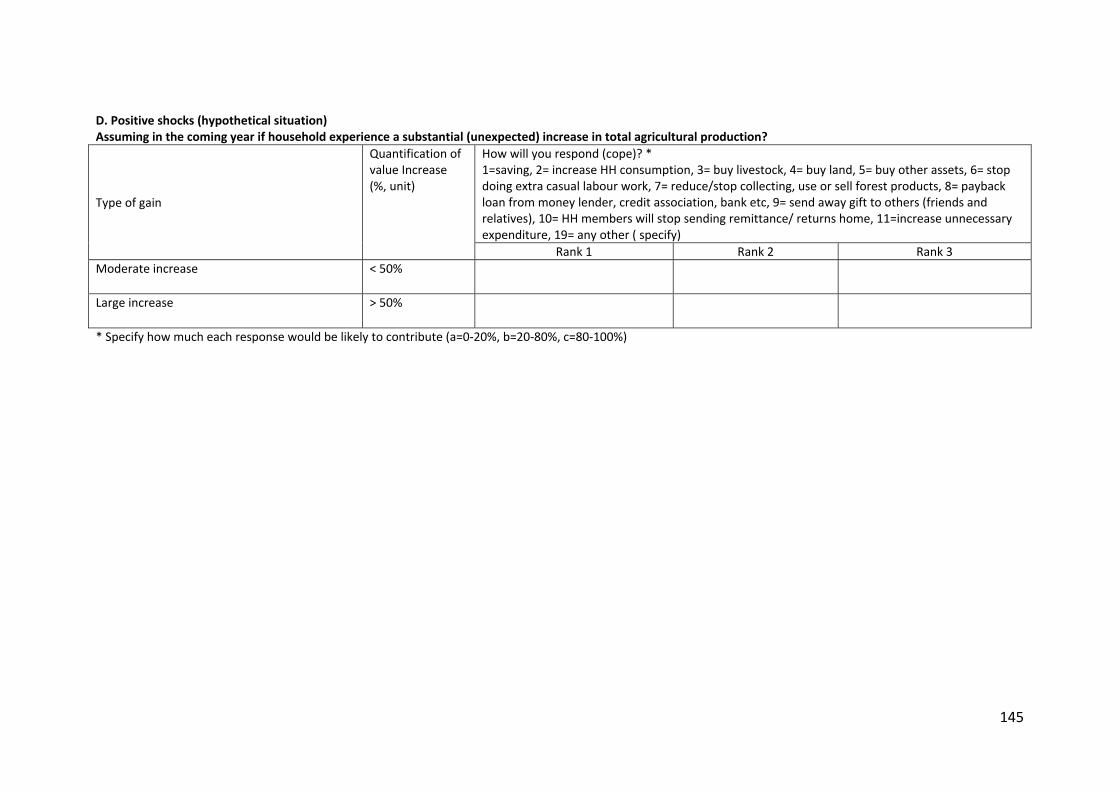
145

 D. Positive shocks (hypothetical situation) Assuming in the coming year if household experience a substantial (unexpected) increase in total agricultural production? 

Type of gain 

Quantification of value Increase  (%, unit) 

How will you respond (cope)? * 1=saving, 2= increase HH consumption, 3= buy livestock, 4= buy land, 5= buy other assets, 6= stop doing extra casual labour work, 7= reduce/stop collecting, use or sell forest products, 8= payback  loan from money lender, credit association, bank etc, 9= send away gift to others (friends and relatives), 10= HH members will stop sending remittance/ returns home, 11=increase unnecessary expenditure, 19= any other ( specify) 

Rank 1 Rank 2 Rank 3

Moderate increase < 50%

Large increase > 50%

* Specify how much each response would be likely to contribute (a=0‐20%, b=20‐80%, c=80‐100%) 

   

146

Appendix II Table AI MLN regression results for coping responses to past situations with an unexpected agricultural income loss 

  Coping responses  1 Spend savings 

  

2 Obtain remittance   

4 Loan or assistance   

5 Sell livestock or land   

6 Work more   

chi2 test  

  Coef.   z  Coef.   z  Coef.   z  Coef.   z  Coef.   z  P > chi2 

No.  Explanatory variables             

1  Household size (AEU)  0.172  1.48  0.703  2.56***  ‐0.0453  0.3  0.0815  0.28  ‐0.0387  0.15  0.0492 

2 No. of adult males in HH (AEU) 

‐0.322  3.09***  ‐0.0894  0.43  ‐0.222  1.64*  ‐0.0298  0.12  ‐0.0613  0.37  0.0615 

3  Farmland owned (ha)  0.0273  0.21  0.104  0.26  0.0293  0.14  ‐0.098  0.26  ‐0.165  0.59  0.973 

4  Livestock  (TLU/AEU)  ‐0.0562  1.45  0.0324  0.24  ‐0.0702  0.96  ‐0.0790  0.8  0.0485  0.42  0.649 

5 Net income from environmental products (USD/aeu)  

‐0.000142  0.19  0.00078  0.4  ‐0.000613 

0.55  ‐0.00584  1.57  0.000815  0.33  0.551 

6 Income from land rented out  

0.00122  0.75  ‐0.245  1.27  0.00381  1.22  ‐0.0416  1.12  ‐0.01478  0.39  0.525 

7 Income quartile: ‘Less poor’ (4)A 

0.386  1.28  ‐0.149  0.17  0.857  2.04**  1.933  2.76***  0.448  0.72  0.0851* 

8 Net business income (USD/AEU) 

0.000585  0.81  0.00164  0.83  ‐0.000416 

0.34  0.000368  0.24  ‐0.00120  0.69  0.221 

9 Pension, support from NGO or government (USD/AEU)  

‐0.00955  3.57***  0.00459  0.57  ‐0.0230  3.49***  ‐0.00945  0.58  ‐0.00277  0.49  0*** 

10  Remittance (USD/AEU)   ‐0.00172  2.7***  0.00242  1.54  ‐0.00148  1.58  ‐0.00704  2.37**  ‐0.00519  2.64***  0*** 

11 Value of all assets (USD/AEU)  

‐6.32E‐05  1.49  ‐3.58E‐05  0.16  ‐0.000200 

2.71***  ‐0.000147  1.02  ‐0.000323  2.01**  0.0695* 

12 Cost of power for irrigation (USD/AEU)  

‐0.0125  1.52  ‐0.0879  0.93  ‐0.0621  2.59***  ‐0.392  2.61***  0.000849  0.03  0.0052*** 

13  Debt (USD/AEU)  0.000318  1.39  0.000902  1.24  0.000136  0.38  0.000569  0.75  0.000495  1.28  0.268 

14  Size of shock B  0.259  1.63  0.00503  0.01  0.217  1.17  0.926  1.96**  0.0239  0.09  0.385 

Constant  ‐0.171  ‐0.42  ‐5.504  3.43***  0.791  1.49  ‐1.419  1.44  0.0974  0.1    

  Number of obs. = 663, Pseudo R2 = 0.0678 

* p<0.1, ** p<0.05, and *** p<0.01  A Dummy variable, takes a value of 1 if the household belongs to income quartile 4 (‘Less poor’) and 0 otherwise.  B Dummy variable, heavy loss (> 50 % ) is 1 and moderate loss (< 50 %) is 0. 

 

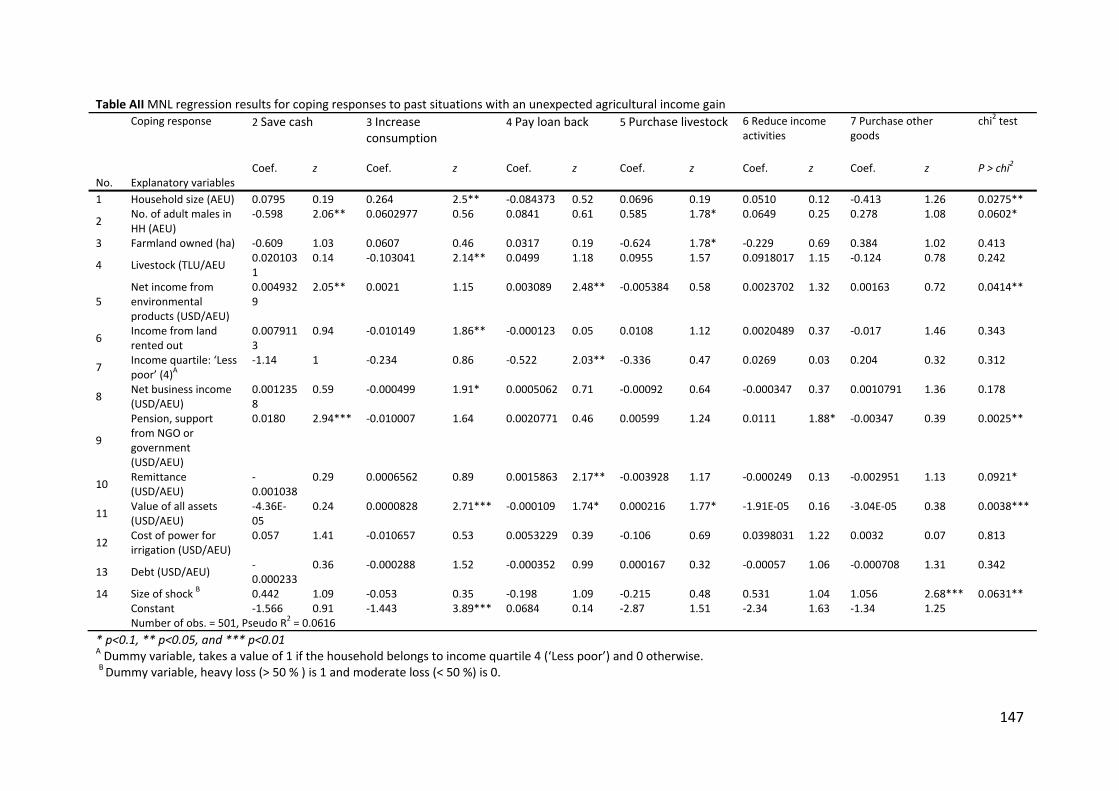
147

Table AII MNL regression results for coping responses to past situations with an unexpected agricultural income gain    Coping response  2 Save cash 

  

3 Increase consumption   

4 Pay loan back   

5 Purchase livestock   

6 Reduce income activities   

7 Purchase other goods   

chi2 test  

    Coef.   z  Coef.   z  Coef.   z  Coef.   z  Coef.   z  Coef.   z  P > chi2 No.  Explanatory variables     

1  Household size (AEU)  0.0795  0.19  0.264  2.5**  ‐0.084373  0.52  0.0696  0.19  0.0510  0.12  ‐0.413  1.26  0.0275** 

2 No. of adult males in HH (AEU) 

‐0.598  2.06**  0.0602977  0.56  0.0841  0.61  0.585  1.78*  0.0649  0.25  0.278  1.08  0.0602* 

3  Farmland owned (ha)  ‐0.609  1.03  0.0607  0.46  0.0317  0.19  ‐0.624  1.78*  ‐0.229  0.69  0.384  1.02  0.413 

4  Livestock (TLU/AEU 0.0201031 

0.14  ‐0.103041  2.14**  0.0499  1.18  0.0955  1.57  0.0918017  1.15  ‐0.124  0.78  0.242 

5 Net income from environmental products (USD/AEU)  

0.0049329 

2.05**  0.0021  1.15  0.003089  2.48**  ‐0.005384  0.58  0.0023702  1.32  0.00163  0.72  0.0414** 

6 Income from land rented out  

0.0079113 

0.94  ‐0.010149  1.86**  ‐0.000123  0.05  0.0108  1.12  0.0020489  0.37  ‐0.017  1.46  0.343 

7 Income quartile: ‘Less poor’ (4)

A ‐1.14  1  ‐0.234  0.86  ‐0.522  2.03**  ‐0.336  0.47  0.0269  0.03  0.204  0.32  0.312 

8 Net business income (USD/AEU) 

0.0012358 

0.59  ‐0.000499  1.91*  0.0005062  0.71  ‐0.00092  0.64  ‐0.000347  0.37  0.0010791  1.36  0.178 

9 

Pension, support from NGO or government (USD/AEU)  

0.0180  2.94***  ‐0.010007  1.64  0.0020771  0.46  0.00599  1.24  0.0111  1.88*  ‐0.00347  0.39  0.0025** 

10 Remittance (USD/AEU)  

‐0.001038 

0.29  0.0006562  0.89  0.0015863  2.17**  ‐0.003928  1.17  ‐0.000249  0.13  ‐0.002951  1.13  0.0921* 

11 Value of all assets (USD/AEU)  

‐4.36E‐05 

0.24  0.0000828  2.71***  ‐0.000109  1.74*  0.000216  1.77*  ‐1.91E‐05  0.16  ‐3.04E‐05  0.38  0.0038*** 

12 Cost of power for irrigation (USD/AEU)  

0.057  1.41  ‐0.010657  0.53  0.0053229  0.39  ‐0.106  0.69  0.0398031  1.22  0.0032  0.07  0.813 

13  Debt (USD/AEU) ‐0.000233 

0.36  ‐0.000288  1.52  ‐0.000352  0.99  0.000167  0.32  ‐0.00057  1.06  ‐0.000708  1.31  0.342 

14  Size of shock B  0.442  1.09  ‐0.053  0.35  ‐0.198  1.09  ‐0.215  0.48  0.531  1.04  1.056  2.68***  0.0631** Constant  ‐1.566  0.91  ‐1.443  3.89***  0.0684  0.14  ‐2.87  1.51  ‐2.34  1.63  ‐1.34  1.25    

  Number of obs. = 501, Pseudo R2 = 0.0616 

* p<0.1, ** p<0.05, and *** p<0.01  A Dummy variable, takes a value of 1 if the household belongs to income quartile 4 (‘Less poor’) and 0 otherwise.  B Dummy variable, heavy loss (> 50 % ) is 1 and moderate loss (< 50 %) is 0. 

148

 Table AIII MNL regression results for coping responses to future unexpected agricultural income loss 

   Coping responses 1 Spend savings   

2 Obtain remittance   

4 Loan or assistance   

5 Sell livestock or land   

6 Work more   

chi2 test  

Coef.   z  Coef.   z  Coef.   z  Coef.   z  Coef.   z  P > chi2 

No.  Explanatory variables             

1  Household size (AEU)  ‐0.142834  1.13  0.217  1.01  0.112  0.58  ‐0.167  0.84  ‐0.256763  1.77*  0.120 

2 No. of adult males in HH (AEU) 

0.0142  0.14  0.072  0.47  0.153  0.97  0.174  1.18  0.221994  2.06**  0.329 

3  Farmland owned (ha)  0.133  0.81  ‐0.029303  0.13  ‐0.270  1.25  ‐0.259  1.14  0.3559243  2.26**  0.0163** 

4  Livestock(TLU/AEU)  0.011  0.32  ‐0.176949  1.29  0.134771  2.14**  0.0494  0.64  ‐0.093048  1.31  0.0034*** 

5 Net income from environmental products (USD/aeu)  

‐0.001996  2.68**  ‐0.005789  3.24***  0.0007614  0.56  ‐0.001502  1.27  ‐0.003017  2.05**  0.0001*** 

6 Income from land rented out  

0.0005305  0.29  0.0131656  2.41**  ‐0.049394  1.16  0.0104  2.26**  ‐0.000806  0.09  0.0074*** 

7 Income quartile: ‘Less poor’ (4)A 

0.0377  0.18  0.9753947  2.63***  ‐0.389  0.94  0.124  0.34  0.28188  0.78  0.0724* 

8 Net business income (USD/AEU) 

0.0010611  2.55**  ‐4.49E‐05  0.05  ‐0.000705  0.73  ‐0.002319  1.74*  0.0007555  1.27  0.0219** 

9 Pension, support from NGO or government (USD/AEU)  

‐0.002878  0.92  ‐0.019173  2.56***  0.0032627  0.86  0.0002198  0.07  ‐0.007559  2.24**  0.0053*** 

10  Remittance (USD/AEU)   ‐0.000215  0.93  ‐0.000741  1.48  ‐0.000374  0.68  ‐0.00171  2.01**  ‐0.000396  1.32  0.211 

11 Value of all assets (USD/AEU)  

‐0.000106  2.91***  ‐0.000187  2.01**  ‐5.95E‐05  0.63  ‐0.000277  2.4**  ‐0.000288  4.29***  0.0003*** 

12 Cost of power for irrigation (USD/AEU)  

‐0.004869  0.4  ‐0.026651  0.87  ‐0.0239  0.67  ‐0.008243  0.3  ‐0.055282  2.03**  0.221 

13  Debt (USD/AEU)  ‐6E‐06  0.03  ‐0.000713  1.35  0.0001342  0.35  0.0003672  1.16  ‐0.000342  1.04  0.067* 

14  Size of shock B  ‐0.236061  1.51  ‐0.656  2.32**  ‐0.826  3.01***  ‐0.057856  0.27  ‐1.341154  7.66***  0 

Constant  0.7511756  1.57  ‐0.654  0.78  ‐1.15  1.52  0.614  0.73  1.98  3.44***    

  Number of obs. = 795, Pseudo R2 = 0.0747     * p<0.1, ** p<0.05, and *** p<0.01  A Dummy variable, takes a value of 1 if the household belongs to income quartile 4 (‘Less poor’) and 0 otherwise.  B Dummy variable, heavy loss (> 50 % ) is 1 and moderate loss (< 50 %) is 0.   

149

Table AIV MNL regression results for coping responses to future unexpected agricultural income gain   

Coping response 2 Save cash   

3 Increase consumption   

4 Pay loan back   

5 Purchase livestock   

6 Reduce income activities   

7 Purchase other goods   

chi2 test  

    Coef.   z  Coef.   z  Coef.   z  Coef.   z  Coef.   z  Coef.   z  P > chi2 

No.  Explanatory variables                           

1  Household size (AEU)  0.312  1.24  0.104  0.9  ‐0.071201  0.64  ‐0.033253  0.26  0.155  0.86  ‐0.301  1.65*  0.214 

2  No. of adult males in HH (AEU) 

‐0.147  0.64  ‐0.127  1.13  ‐0.011066  0.11  0.217  1.73*  ‐0.031443  0.24  0.082  0.57  0.278 

3  Farmland owned (ha) 

‐0.935  2.47  ‐0.190  1.3  0.0120  0.09  ‐0.128  0.77  ‐0.753  2.25**  0.0143  0.06  0.009*** 

4  Livestock (TLU/AEU)  ‐0.107  0.86  0.0198  0.6  ‐0.0116  0.26  ‐0.046514  1.21  ‐0.219  2.05**  ‐0.010676  0.2  0.362 

5  Net income from environmental products (USD/aeu)  

‐0.000524  0.22  0.0017254  2.14**  ‐0.000627  0.68  ‐0.000747  0.5  ‐0.000218  0.13  ‐0.003473  2.24**  0.0007*** 

6  Income from land rented out  

0.0139  2.25**  ‐0.011626  2.5**  ‐0.00375  0.47  0.0008113  0.35  0.0062052  1.36  0.0017984  0.35  0.0005*** 

7  Income quartile: ‘Less poor’ (4)A 

‐0.247  0.35  0.102  0.4  0.255  0.93  0.445  1.43  0.320  0.66  ‐0.292  0.72  0.610 

8  Net business income (USD/AEU) 

‐0.001875  1.11  ‐0.000452  0.8  ‐0.0005  0.67  ‐0.001627  2.3**  ‐0.002123  1.9*  0.0015093  3.59***  0.0002*** 

9  Pension, support from NGO or government (USD/AEU)  

‐0.002173  0.17  0.0052955  1.23  0.0020825  0.39  0.0016789  0.34  0.0065078  1.18  0.0071337  0.99  0.186 

10  Remittance (USD/AEU)  

‐0.000738  0.68  0.0001429  0.6  ‐0.000383  1.23  ‐0.001537  2.11**  ‐0.00063  0.89  ‐9.55E‐05  0.2  0.251 

11  Value of all assets (USD/AEU)  

0.0001304  1.02  0.000055  1.33  ‐0.000126  1.92*  0.0000842  1.89*  0.0000731  0.79  ‐6.63E‐05  1.4  0*** 

12  Cost of power for irrigation (USD/AEU)  

0.0061305  0.16  0.0235577  1.61  ‐0.02448  0.89  ‐0.068008  2.03**  0.0112  0.35  ‐0.032035  0.99  0.0049*** 

13  Debt (USD/AEU)  0.000372  0.6  ‐6.79E‐05  0.31  ‐0.000427  1.39  ‐0.000159  0.53  0.0001236  0.24  ‐0.000233  0.66  0.238 

14  Size of shock B  2.19  4.51***  ‐0.041701  0.23  1.021  5.11***  0.781  3.79***  0.827  3.05***  0.421  1.48  0*** 

  Constant  ‐3.13  3.28***  ‐0.204068  0.49  0.562  1.35  ‐0.602  1.39  ‐0.955  1.28  0.183  0.26   

  Number of obs. = 787, Pseudo R2 = 0.0569 

* p<0.1, ** p<0.05, and *** p<0.01  A Dummy variable, takes a value of 1 if the household belongs to income quartile 4 (‘Less poor’) and 0 otherwise.  B Dummy variable, heavy loss (> 50 % ) is 1 and moderate loss (< 50 %) is 0. 

150  

Paper 4  

  

Simulation of Optimal Decision‐Making under the Impacts of Climate Change  Lea Ravnkilde Møller1, Martin Drews2, and Morten Andreas Dahl Larsen2 

1UNEP  DTU  Partnership,  DTU  Management  Engineering,  Technical  University  of  Denmark, 

Marmorvej 51, DK‐2100 Copenhagen, Denmark  

2Department of Systems Analysis, DTU Management Engineering, Technical University of Denmark, 

Produktionstorvet, building 426, DK‐2800 Kgs. Lyngby, Denmark 

Submitted, November 2016, to Environmental Management. 

Key words: Bayesian updating, Monte Carlo simulation, climate change, adaptation, agriculture, 

uncertainty 

 Abstract  Climate change causes transformations to the conditions of existing agricultural practices appointing farmers  to  continuously  evaluate  their  agricultural  strategies  towards  optimizing  revenue.  In  this light,  this  paper  presents  a  framework  for  applying  Bayesian  updating  to  study  decision‐making, reaction patterns and updating of beliefs among farmers  in a developing country, when faced with the complexity of adapting agricultural  systems  to climate change. The approach  is applied on an example in which a farmer in Ghana, holding an initial belief, seeks to decide on the most profitable of three agricultural systems (dryland crops, irrigated crops and livestock) by a continuous updating of beliefs relative to realised trajectories of climate (change), using the variables of temperature and precipitation.  The  climate  data  is  based  on  combinations  of  output  from  three  global/regional climate model combinations and two future scenarios (RCP4.5 and RCP8.5) representing moderate and unsubstantial GHG reduction policies respectively.  The results show that the climate scenario (input) holds a significant influence to the development of beliefs,  net  revenues  and  thereby  optimal  farming  practice.  Also,  despite  uncertainties  in  the underlying net revenue functions, the results show that when the beliefs of the farmer (the decision‐maker)  opposes  the  direction  of  the  realised  climate  development,  Bayesian  updating  of  beliefs allows  for  an  adjustment  of  such  beliefs,  as more  information  becomes  available  to  the  farmer, helping  him make  the  optimal  choice  between  agricultural  systems  considering  the  influence  of climate change.  

 

151  

Introduction 

 

The UN Intergovernmental Panel on Climate Change (IPCC) states that the climate system is warming 

and  that  anthropogenic  drivers  are  extremely  likely  to  have  been  the  dominant  cause  of  the 

observed warming since the mid‐20th  (IPCC 2013). The evidence of climate change  is unequivocal, 

and it is likely that further warming will increase the "likelihood of severe, pervasive and irreversible 

impacts  for people and ecosystems"  (IPCC 2014). Thus, climate change represents a serious global 

risk, which demands an urgent global response (e.g. Stern 2006). Arguably, climate change will have 

the greatest effect on the poorest and most vulnerable developing countries and population groups 

(Das Gupta  2014,  IPCC  2014). Many  parts  of  the  developing world  are  thus  likely  to  experience 

climate‐induced declines  in  agricultural output, poorer health  conditions, modifications of  rainfall 

patterns,  and more  frequent  natural  disasters  e.g.  floods, droughts or  storms. As  a  consequence 

some  areas  will  be  rendered more  or  less  habitable  or  inhabitable,  and  poverty  reduction  and 

economic growth will be severely hindered. 

One characteristic of the changing climate is that projections of climate change even for short time 

horizons  are  associated with  a high  degree of uncertainty  (e.g. Refsgaard  et  al.  2013),  stemming 

from different sources such as model uncertainty (e.g. Hawkins and Sutton 2011, Larsen et al. 2013), 

scenario uncertainty (e.g. Yip et al. 2015), natural variations (e.g. Deser et al. 2012), and incomplete 

knowledge of the climate system (e.g. Oreskes et al. 1994). This aggregated uncertainty and the best 

responses  here  to,  are  not  easily  identified  through  observed  time  series  of  past  climate  and  its 

systemic  impacts, nor through more dynamic approaches,  including experiments of trial‐and‐error. 

Rather, we are likely to learn about the actual realization of climate change only as time passes, and 

in particular at the detailed  level. This  is true not only for changes  in, e.g. precipitation patterns or 

the severity of droughts, but also for drivers of these changes (e.g. greenhouses gas emissions), and 

the uncertainty of  these  factors.  Likewise,  the potential  impacts of  climate  change are associated 

with high uncertainty, e.g. the resulting agricultural yields are conditioned not only on climate but 

also on  the  installed adaptive measures, management practices and  technologies, etc. Conversely, 

traditional  economic  approaches  towards  characterising  such  uncertainty  rely  almost  entirely  on 

past  experiences,  e.g.  the  real  option  literature,  where  you  estimate  the  value  gained  from 

additional information before making an irreversible investment (Arrow and Fischer 1974; Simal and 

Ortega 2011).  

152  

Risk and uncertainty are central concepts for decision‐making on both mitigation and adaptation to 

climate  change. Where  'risk'  generally  refers  to  cases where  the  probability  of  outcomes  can  be 

ascertained  through well‐established  theories and  the availability of suitable data,  'uncertainty' as 

mentioned above  refers  to  situations where appropriate data may be  fragmentary or unavailable 

(Halsnæs et al. 2007). Climate change scenarios used by e.g.  the  IPCC  (2014) cannot  in general be 

assigned with accurate numerical probabilities. Instead conclusions are expressed in terms like "very 

likely", which may  again  be  transferred  to  an  approx. numerical  value  (e.g.  ">  90% probability"). 

Budescu,  Broomell  and  Por  (2009)  have  criticised  the  IPCC  for  not  explicitly  considering  the 

numerical probability of climate change, and they conclude that the consequence of this lack is that 

different  people  will  interpret  the  probability  terms  differently,  regardless  of  the  international 

guidelines.  This  in  turn may  skew  decisions  and  introduce  significant  ambiguity,  since  risk‐based 

methods are widely used to analyse decision‐making in connection with climate change (Vardas and 

Xepapadeas  2010;  Klibanoff,  Marinacci  and  Mukerji  2003).  As  a  result  the  decision‐maker's 

capabilities and personal bias can play a significant role  i.e.  in the  interpretation of the occurrence 

that are most  likely  to happen  in  the  future  (or  in  the decision‐makers' expectation of  the  future) 

and are often compounded by his/her level of 'risk aversion'.  

In the following we use the methodology of Yousefpour et al. (2014, 2015) to simulate an adaptive 

decision‐making, addressing  the abovementioned complexity of making  'optimal' decisions  for  the 

future under the  influence of climate change. This  includes the difficult  issue of timing, that  is, the 

process of determining when a decision‐maker  (here:  the  farmer)  should  shift his  focus  from one 

(agricultural)  system  to another. Basically,  the  idea  is  that a decision‐maker holds an  initial  set of 

subjective beliefs of  the  likelihood of various climate  realizations  that  for completeness add up  to 

one.  As  time  passes,  an  adaptive  decision maker  will  observe  the  development  of  the  climate, 

enabling  him  or  her  to  gradually  adapt  choices.  For  this  aim  Yousefpour  et  al.  (2014,  2015) 

introduces  a  Bayesian  methodology  for  updating  the  decision‐makers  beliefs  towards  different 

climate  realizations  based  on  observations.  The  framework  makes  it  possible  to  simulate  the 

trajectory of learning and reaction patterns among decision‐makers in examples where the situation 

does not develop as expected or predicted. An everyday example of a gradually adaptive decision‐

making, based on experience could be: should  I bring an umbrella when walking to work? To start 

with,  I might  always  bring my  umbrella,  but would  gradually  experience  that  it  is  rarely  needed 

thereby instigating an adaptation to how often, or even when, an umbrella should be brought.  

The  framework  for Bayesian updating we have applied matches  the process of choosing between 

agricultural  systems  as  climate  change  adaptation,  and  through  this  point  out  the  advantages  of 

153  

proactive adaptation (ex ante – avoid learning by shock [Tschakert and Dietrich 2010]) over reactive 

adaptation  (ex  post  –  learning  by  shock)  to  climate  change.  Several  authors  find  that  proactive 

adaptation  activities  can  provide  significant  welfare  gains  and  resilience  to  climate  change  at 

household level (Boko et al. 2007). Similarly, reactive adaptation can in the long run contribute with 

proactive initiatives by adding to the pool of knowledge on how to deal with climate change (Lecocq 

and Shalizi 2007). Fankhauser, Smith and Tol  (1999) also highlight  that  the  line between proactive 

and reactive adaptation can be blurred when working within a dynamic setting. Thus  in this paper 

we will also try to capture the  irreversible decisions that must be made to create more permanent 

adaptation  strategies,  as  opposed  to  temporary  coping  strategies  and  autonomous  adaptation 

initiatives.  

To  illustrate  the  methodological  aspects  of  decision‐making  we  have  used  the  example  of  a 

representative farmer's choice of agricultural system in Ghana as adaptation to climate change, e.g. 

simulating  reaction  patterns  among  farmers  as  a  response  to  observations  of  the  'real'  climate 

developments.  As  a  result  the  farmer may  opt  to  change  his  choice  of  agricultural  system,  as  a 

response to observations, and he builds confidence  in climate projections by experiencing changes 

over  time.  This makes  it  possible  to  determine which  future  choices  are  optimal, when  the  true 

climate trajectory is revealed over time.  

The  example  of  a  representative  farmer  represents  a  hypothetical  decision‐making  problem,  and 

indicates how every day (potentially irreversible) decisions can be biased by a wide range of factors. 

While  climate  change  impacts may  involve  adjustments  from  season  to  season  for  some  crops 

(autonomous  adaptation),  some  changes will  require  adjustments  to  the  agricultural  production 

system as such, which may not be easily reversible  in the short run. Technically  it may be possible, 

but  the  costs would be  too high  for  the  farmer  in  the  short  run, and any  changes  to agricultural 

systems can be said to be based on a medium‐ to long‐term strategy, at least implicitly. This may of 

course result in new pressures on common land for grassing and on water for irrigation, or it may be 

seen as an on‐going process of choosing which  land  should be allocated  to  the different  systems. 

Hence in real life farmers may use several agricultural systems on different pieces of land.   

 

   

154  

Adaptation to Climate Change in African Agriculture 

 

The potential impacts of climate change on African agriculture are expected to be severe and lead to 

significant  losses  in the aggregated production without the  implementation of effective adaptation 

(Challinor  et  al.  2014).  Hence  the  projected warming  combined with  e.g.  reduced  and/or  highly 

variable future rainfall patterns  is expected to have  large effects on select crop types. At the same 

time the adoption of modern technologies in many parts of Africa, including Ghana, is low, and the 

local economies highly dependent on agriculture. On  the other hand,  several  studies  suggest  that 

suitable adaptation measures may reduce these negative  impacts of climate change on agriculture 

and crop yields (Antwi‐Agyei et al. 2012; Antwi‐Agyei, Stringer and Dougill 2014; Antwi‐Agyei, Dougill 

and  Stringer  2015;  Benhin  2008;  Boko  et  al.  2007).  For  example  Boko  et  al.  (2007)  argue  that 

proactive adaptation may result in welfare gains and resilience to climate change on the household 

level,  as opposed  to Benhin  (2008) who  indicates  that without adaptation  the net  crop  revenues 

concentrated  in South Africa are  likely to fall by as much as 90 percent over the course of the 21st 

century, and that climate change will have the greatest impact on small‐scale farmers.  

In case studies  from north‐eastern Ghana, Antwi‐Agyei, Dougill and Stringer  (2015)  identify a poor 

development of the necessary infrastructure, prevention of market access and missing access to new 

drought‐tolerant  species  as  some  of  the  key  barriers  towards  climate  change  adaptation  in  the 

region.  Their  studies  further  show  how  the  barriers  can  be  as  simple  as  lack  of  information  on 

adaptation options and of understanding the need for implementing adaption initiatives. Hence not 

all farmers are aware of climate change and the consequences they can have in the long run. Antwi‐

Agyei, Dougill and Stringer (2015) conclude that it is critically important to address these barriers to 

be  able  to  successfully  implement  climate  change  adaptation  in  the  agricultural  sector.  In  this 

context  Boko  et  al.  (2007)  along with  Antwi‐Agyei,  Stringer  and  Dougill  (2014)  and  Antwi‐Agyei, 

Dougill  and  Stringer  (2015)  all  propose  that  proactive  approaches  enhances  the  adaptation  to 

climate change. Importantly, they also find that farmers are willing to implement on‐farm adaptation 

strategies  and  that  their  decisions  highly  depend  on  observations  of  present  climatic  conditions. 

Hence Boko et al.  (2007) show  that  farmers  in Africa  tend  to select crops  that are adapted  to  the 

current climate in their region, and that they tend to shift towards more heat‐tolerant crops, as the 

weather becomes warmer.  Likewise, an  increase or decrease  in precipitation makes  farmers  shift 

towards more water‐loving or drought‐tolerant species, assuming they are available to the individual 

farmer. 

155  

Evidently, the key to overcoming some of the barriers mentioned may be to find a balance between 

flexibility (e.g. the opportunity of switching to different types of crops), reducing the vulnerability of 

the agricultural systems and optimizing the returns obtained by  individual farmers. Different crops 

require different conditions to produce the highest returns. Switching from one agricultural system 

to another may involve cost and time lags before new crops yield a profit, causing some decisions to 

be effectively irreversible, and some crops may perform more inconsistently than others with regard 

to revenues in the face of climate change.  

How to address the trade‐offs between these different aspects in an evolving climate is the focus of 

this  paper.  In  the  paper  we  discuss  key  issues  related  to  adaptation  decision‐making  using  a 

probabilistic framework that simulates how to make an 'optimal' choice of agricultural system which 

may or may not change dynamically over time, as information about the future climate trajectory is 

revealed,  and  compounded by  the  initial  and  shifting  expectations of  the  farmer. Combined,  this 

yields a numerical simulation of the decision‐makers' learning trajectory, in this example a farmer's, 

to allow us to investigate explicitly the roles of learning and user preferences in adaptation decision‐

making, which may be critical  in  terms of designing effective adaptation  strategies, but which are 

often ignored by integrated decision‐support systems.   

 

Methods and Data  

 

To  simulate  how  management  decisions  may  change  when  new  and  potentially  improved 

information becomes available we employ the same methodology as Yousefpour et al. (2014, 2015). 

Yousefpour et al.  (2014, 2015)  introduces a Bayesian methodology  for modelling numerically how 

the  'beliefs' of  local  forest managers,  i.e.  in a certain  future climate development  (represented by 

three  different  climate  model  projections),  are  updated  as  simulated  observations  of  mean 

temperature, minimum  temperature  and mean  precipitation  are  drawn  from  the  'true'  climate 

trajectory  (initially  unknown  to  the  decision‐maker)  and  becomes  available  over  time.  Following, 

they then discuss best management strategies at three different points  in time conditioned by the 

managers' beliefs at  those points  in  time, whether  their behaviour  is  'actively‐adaptive' or not, as 

well  as  local  conditions  and  forest  characteristics,  e.g.  the  performance  of  select  tree  species  as 

defined by a forest  landscape model, the available management options and existing management 

schemes, ownership types, etc.   

156  

In this study we adopt a different approach to better reflect the reality of a Ghanaian farmer’s choice 

of  agricultural  system  under  climate  change.  The  farmer's  beliefs  are  here  updated  based  on 

simulated observations of annual mean temperature and precipitation. Since crops are annual and 

thus easier  to replace we consider short  five‐year  time slices as  the baseline  for decisions on new 

management strategies, which we simply define as a choice of 'dryland farming' (i.e. rain fed crops), 

'irrigated farming' or 'livestock' as in Kurukulasuriya et al. (2006) For this aim we initially carry out a 

detailed analysis of  state‐of‐the‐art  regional  climate model projections  for Ghana e.g.  to properly 

account also for changes in inter annual variations of temperature and precipitation in our choice of 

climate realizations, which may have profound  impacts on the agricultural performance and hence 

adaptation decisions on these time scales. Finally we use the net revenue per farm for each type of 

agricultural system, calculated using the Ricardian method of Kurukulasuriya et al. (2006), as the sole 

determinant of optimal decisions on adaptation. In line with this model we do not explicitly consider, 

e.g. crop characteristics as part of our decision‐space, and neither  local soil types, water resources 

availability, etc. as these are more or less implicit in the model by Kurukulasuriya et al. (2006).  

 

Updating Beliefs Using Bayesian Analysis  

As  in  Yousefpour  et  al.  (2015) we  simulate  how  the  farmer's  beliefs  concerning  three  different 

climate model projections, selected from a larger ensemble (see below), would change in the period 

from 2015 to 2085 as new annual observations of the actual climate development emerge. Let Wit 

indicate  the  farmer's  belief  that  a  particular  climate  projection  (i)  from  a  selection  of  (n  =  3) 

ensemble members will be realized in the year t, and that the sum of his beliefs is normalized to one 

as if they were probabilities (Equation 1): 

 

∑ 1 , 0forall , .            (1) 

 

Thus, if a farmer truly believes in specific climate projection j then his belief towards this realization 

is given by wjt=1 while wit=0 for ij. We assign the farmer's initial beliefs wi0 to the year 2015. 

We use Bayes’ theorem (Bayes and Price 1763)  iteratively to update the farmer's belief every year 

from 2016‐2085. Assuming xt0  to be an estimate  (observation) of  the  state of  the climate  (annual 

mean  temperature,  annual  mean  precipitation)  randomly  drawn  from  a  multivariate  normal 

distribution centred around the 'true' realized climate development (here: as simulated by a climate 

157  

model), then the updated beliefs (probabilities) at time t+1 related to the situation at time t for each 

of the n=3 different climate model projections is given by (Equation 2): 

 

n

iii

ot

iioto

tiotti

tx

txxxw

1

1,

),modelPr(modelPr

),modelPr(modelPrmodelPr)(

    (2) 

 

where  the  updated  belief  , Pr |   is  the  probability  of  climate  projection  i 

representing  the  true  realization  of  climate  change  given  the  observation  xt0  at  time  t, 

Pr |   is  the  probability  that  the  observation  xt0  is  drawn  from  the  distribution  centred 

around climate projection i at time t, and Pr ,  is the probability of modeli representing the 

real  climate  development  at  time  t. Using  Equation  2 we  can  update  our  beliefs  in  each  of  the 

alternative climate projections, provided we know  what the real climate development will be. In the 

present analysis we select each of  the  three different climate projections  in  turn  to  represent  the 

real  climate,  e.g.  a  'perfect' model  approach.  Realistically,  none  of  the  three  climate  projections 

however will mimic exactly  the  real climate and hence one could also have chosen an alternative 

approach, where e.g. a fourth projection would represent the actual climate.    

For simplicity, we assume that the simulated observations of annual mean temperature and annual 

mean precipitation are drawn  from a multivariate normal distribution centred on  the  real climate 

realization (Equation 3),  

 

~ ̅ , , ,           (3) 

 

where  temp  and  prec  in  Equation  3  are  calculated  from  running  30‐year  time  slices  of  projected 

annual  temperature  and  precipitation  produced  by  a  climate model  centred  on  the  consecutive 

observation points  (2020, 2025, …, 2085) used  for  the management analysis discussed below, and 

Cov(…)  is  the  symmetric and positive definite  covariance matrix  calculated  from  the annual mean 

temperature  and  precipitation  series.  Using  running  time  slices  rather  than  estimating  the 

covariance matrix  from  the  full  time  series  as  done  by  Yousefpour  et  al.  (2015)  allows  for  the 

simulated  climate  to exhibit natural  variations  consistent with  the  climate model projections  and 

158  

adequate  for  considering  five‐year  periods.    Hence  in  the  real  climate  system  decadal  or multi‐

decadal variations occur, e.g. extended periods of more or  less precipitation, which may partly or 

wholly overlap any five‐year period, used in this study to represent the observation time used by an 

African farmer to decide on changing his management practices. As a result his belief update which 

is based on new observations of  the present  climate  conditions  is  likely  to be  influenced by  such 

natural  climate variations.   Using a 30‐year  time  slice as  the basis  for estimating  the  inter annual 

covariance  is consistent with current practices amongst climate and weather modellers, where 20‐ 

or 30‐year averages are also considered as the base for calculating e.g. climate normal or changes to 

climate variables in a future climate (assuming approximate stationarity). 

The probability distribution of the multivariate normal distribution for annual mean temperature 

and precipitation is defined by Equation 4 with k=2 and the rest of the terms as defined above.  

 

Pr |, /

∙ exp 1/2 ̅ , ̅     (4) 

 

In our simulations we repeated the belief update from 2015 to 2085, performing random draws at 

every  annual  time  step,  a  total  of  200  times  (or  14000  annual  draws  all  together).  Additional 

repetitions > 200 were not found to change our results significantly. The Monte Carlo procedure was 

coded in Matlab, and the run time for a single experiment was less than a minute. 

  

Climate Scenarios  

To  represent  different  possible  climate  realizations  we  use  precipitation  and  (near  surface  air) 

temperature  output  from model  combinations  in  the  COordinated  Regional  climate Downscaling 

EXperiment (CORDEX) database (Nikulin et al. 2012). In CORDEX, output from a substantial number 

of  regional  climate models  (RCMs)  forced    on  the  boundaries  of  their model  domains  by  global 

climate models or earth system models (for simplicity here referred to jointly as GCMs), delivered by 

numerous climate research  institutes, are available across 14 different domains, which cover most 

regions  of  the  world.  To  select  three  members  representing  different  climate  realizations,  we 

assessed differences  in model performance  in  terms of absolute and  residual values,  inter annual 

variability,  year‐to‐year  amplitudes  and  projected  future  trajectories  from  each  of  the  available 

RCMs  over  the African model  domain,  covering  the  entire  continent.  For  RCM  driven  by  several 

GCMs, one  random RCM output was  chosen except  for one RCM  (CCLM4)  to here also  study  the 

influence of  the GCM.  This  resulted  in data being  extracted  from  the  seven model  combinations 

shown in table 1. Climate data for both the available historical period (1951‐2005) and the projected 

159  

future  (2006‐2100)  were  used.  Annual  mean  temperature  and  precipitation  anomalies  were 

calculated  using  a  reference  period  of  1979‐2005.  Both  the  (Representative  Concentration 

Pathways) RCP4.5  and RCP8.5  trajectories  (IPCC  2013) were  considered  in order  to  span  a wider 

range  of  climate  realizations  and  include  scenarios  of  both  intermediate  as  well  as  high  future 

greenhouse gas emissions (GHG). The gridded data were extracted on a yearly basis and processed 

into a spatial mean for Ghana based on grid cells from the CORDEX domain in the latitude‐longitude 

range of 5.7o N to 11.0 o N and 2.6o W to 0.4o E respectively.     

To assess also the sub‐annual scales, the climate data were further analysed for changes in monthly 

values (not shown) as opposed to the annual means. A very limited agreement between the models 

was seen except for temperature in the RCP8.5 scenario where the temperature increase (as seen in 

annual values for figures 1 and 2) is generally stronger in the months November‐June as opposed to 

July‐October.      

In  the  historical  period  annual mean  temperatures  generally  increase  from  approx.  25oC  around 

1950 to approx. 25.5 oC around 2005 (figure 1). Here the CRCM and RACMO models however differ 

with  absolute  values  of  approx.  24oC  and  23oC  increasing  to  approx.  25oC  and  23.5oC,  indicating 

systematic biases of a different order of magnitude than the other models. For the RCP4.5 scenario 

average values  increase steadily reaching approx. 27oC around 2070, followed by a generally  lower 

increase  reaching  approx.  27.5oC  in  2100.  The CRCM  and RACMO models  also  exhibit  systematic 

biases for the RCP4.5 scenario, showing lower values reaching approx. 26.5oC and 25oC in 2100 and 

with  CRCM  even  showing  a  slight  decrease  in  2070‐2100.  For  the RCP8.5  scenario, mean  annual 

temperatures  of  approx.  30oc  are  seen  by  2100 within  the  range  of  29‐31oC  except  for  RACMO 

reaching approx. 27oC. For both RCP scenarios the  largest amplitudes of  inter annual variations are 

found for the MPI‐CCLM model. 

 

160  

  

Figure 1 Mean annual temperature output (absolute and residual) over Ghana extracted from the CORDEX 

database as used to force the decision‐making model. Output from the available historical period (1951‐2005) 

and the RCP periods used (RCP4.5 and RCP8.5) (2006‐2100). The three scenarios used (C1‐C3) are highlighted 

in colours. 

 

 

 

Figure 2 Precipitation output, same as for figure 1, mm precipitation per year. 

 

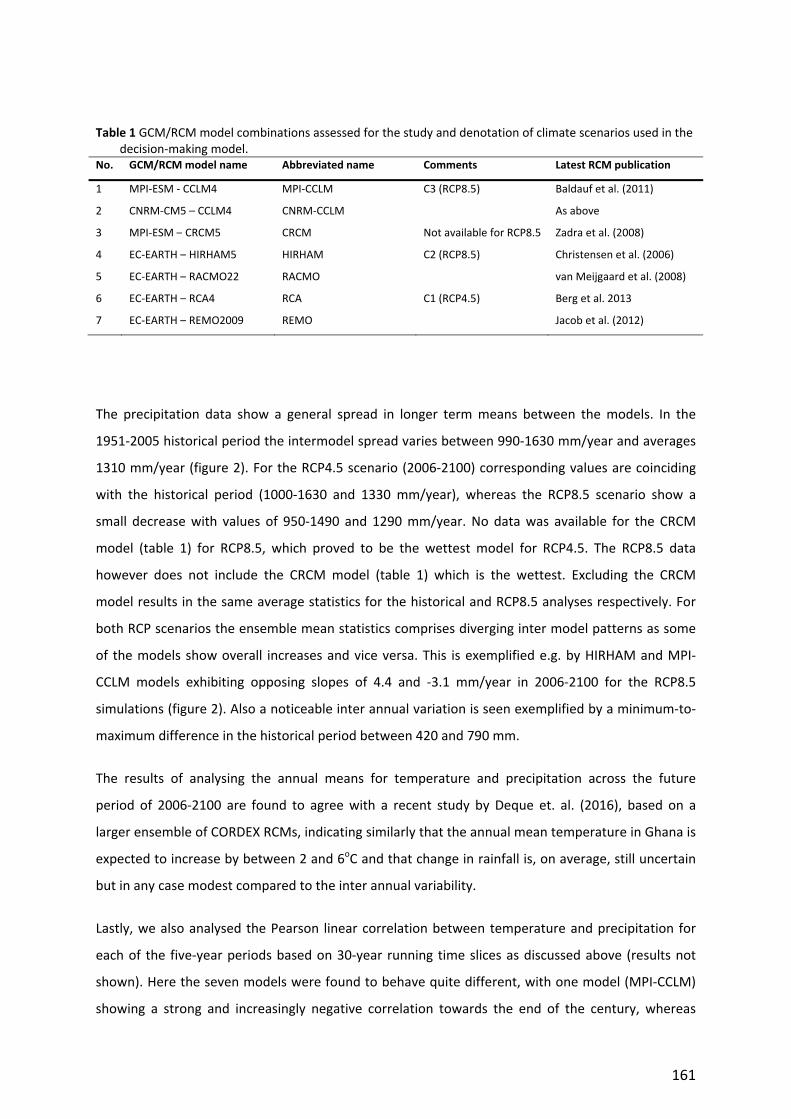
161  

 

Table 1 GCM/RCM model combinations assessed for the study and denotation of climate scenarios used in the decision‐making model. 

No.  GCM/RCM model name  Abbreviated name Comments Latest RCM publication

1  MPI‐ESM ‐ CCLM4  MPI‐CCLM  C3 (RCP8.5) Baldauf et al. (2011) 

2  CNRM‐CM5 – CCLM4  CNRM‐CCLM As above 

3  MPI‐ESM – CRCM5  CRCM  Not available for RCP8.5  Zadra et al. (2008) 

4  EC‐EARTH – HIRHAM5 HIRHAM  C2 (RCP8.5) Christensen et al. (2006)

5  EC‐EARTH – RACMO22 RACMO  van Meijgaard et al. (2008)

6  EC‐EARTH – RCA4  RCA  C1 (RCP4.5) Berg et al. 2013 

7  EC‐EARTH – REMO2009 REMO  Jacob et al. (2012) 

 

 

The precipitation data  show  a  general  spread  in  longer  term means between  the models.  In  the 

1951‐2005 historical period the intermodel spread varies between 990‐1630 mm/year and averages 

1310 mm/year (figure 2). For the RCP4.5 scenario (2006‐2100) corresponding values are coinciding 

with  the  historical  period  (1000‐1630  and  1330 mm/year), whereas  the  RCP8.5  scenario  show  a 

small decrease with values of 950‐1490 and 1290 mm/year. No data was available  for  the CRCM 

model  (table  1)  for  RCP8.5, which  proved  to  be  the wettest model  for  RCP4.5.  The  RCP8.5  data 

however  does  not  include  the  CRCM model  (table  1) which  is  the wettest.  Excluding  the  CRCM 

model results  in the same average statistics for the historical and RCP8.5 analyses respectively. For 

both RCP scenarios the ensemble mean statistics comprises diverging inter model patterns as some 

of  the models show overall  increases and vice versa. This  is exemplified e.g. by HIRHAM and MPI‐

CCLM models  exhibiting  opposing  slopes  of  4.4  and  ‐3.1 mm/year  in  2006‐2100  for  the  RCP8.5 

simulations (figure 2). Also a noticeable inter annual variation is seen exemplified by a minimum‐to‐

maximum difference in the historical period between 420 and 790 mm. 

The  results  of  analysing  the  annual means  for  temperature  and  precipitation  across  the  future 

period of 2006‐2100  are  found  to  agree with  a  recent  study by Deque et.  al.  (2016), based on  a 

larger ensemble of CORDEX RCMs, indicating similarly that the annual mean temperature in Ghana is 

expected to increase by between 2 and 6oC and that change in rainfall is, on average, still uncertain 

but in any case modest compared to the inter annual variability.   

Lastly, we also analysed  the Pearson  linear correlation between  temperature and precipitation  for 

each of  the  five‐year periods based on 30‐year running  time slices as discussed above  (results not 

shown). Here the seven models were found to behave quite different, with one model (MPI‐CCLM) 

showing  a  strong  and  increasingly  negative  correlation  towards  the  end  of  the  century, whereas 

162  

other models  showed positive  correlations or no  trend  at  all. Based on  the  combined  results we 

finally selected three climate projections to be used for the further analyses, reflecting the full span 

of possible climatic outcomes. As low emission and low impact scenario we selected the RCA model, 

downscaling the RCP4.5 scenario (hereafter entitled C1), to constitute a ‘baseline’ climate of minimal 

change. The second scenario (HIRHAM, RCP8.5 – entitled C2) was chosen due to being wetter than 

most,  representing  a  temperature  increase  in  the  lower  range  of  the models  included  here,  and 

exhibiting a positive temperature‐precipitation. Conversely, the third scenario (MPI‐CCLM, RCP8.5 – 

entitled C3) was selected for being the driest, having the highest temperature increase by the end of 

the century and a strong negative temperature and precipitation correlation. 

 

Agricultural Systems 

We assume for simplicity that the farmer's principal objective is to maximise the net revenue of his 

agricultural activities. For this aim we adopt the economic model developed by Kurukulasuriya et al. 

(2006) and apply this to Ghana.  In this cross‐sectional approach the relationships between climate 

and net revenues from three different agricultural systems: dry crops,  irrigated crops and  livestock 

are studied using a standard Ricardian model formulation for each agricultural system. Based on an 

ordinary  least  squares  regression  and  using  the  results  of  e.g.  more  than  9,000  farm  surveys 

conducted  in 11 different countries  in Africa (including  information on water flows,  local soil types 

and a variety of economic variables), the marginal climate impacts on net farm revenues per farm (in 

USD) as estimated by Kurukulasuriya et al. (2006) are reproduced in table 2. 

 Table 2 Marginal climate impacts on net revenue per farm (US Dollars/USD) based on data presented by Kurukulasuriya et al. (2006). Ordinary Least Square (OLS) numbers in parentheses are the maximum and minimum coefficients (95% confidence intervals).  ** p<0.05, and *** p<0.01. Marginal impact  Dryland crop Irrigated crop Livestock

OLS   

Temperature  ‐239*** (‐335, ‐142) 3005 (‐2040, 8048) ‐379 (‐775, 17)

Precipitation  15*** (5.1, 25) 301.3 (‐896.6, 1499.3) 19.9** (0.3, 39.5)

 

The marginal effect of changes in precipitation specified by the coefficients in table 2 corresponds to 

an  increase  in the annual mean precipitation of 1 mm  (calculated  from monthly means). Similarly, 

the marginal  effect  of  changes  in  temperature  corresponds  to  an  increase  in  the  annual mean 

temperature  of  1oC.  The  baselines  for  these  estimates  were  set  by  time  series  of  climate 

observations  spanning  1988‐2003  (temperature)  and  1977‐2000  (precipitation).  The  numbers  in 

parenthesis  indicate  the  95%  confidence  intervals  and  will  in  the  following  be  referred  to  as 

163  

minimum  respectively  the maximum  coefficients.  For more  details  about  the model  a  detailed 

description is provided in Kurukulasuriya et al. (2006). 

The main  advantage of  the  regression  type model by Kurukulasuriya  et  al.  (2006)  is  that  the net 

revenues revealed by their analyses  in a simple way reflects the benefits and costs of autonomous 

adaptation and coping strategies, such as the choice of sowing method and timing. This  includes a 

variety of contributions and the introduction of substitute actions, which farmers have incorporated 

in  order  to  adapt  to  the  current  climate  viabilities.  As  a  result  it  is  readily  possible  within  the 

framework  to  simulate  an  irreversible  decision,  as  autonomous  adaptation  is  already  included. 

Labour costs have not been  included, since  the shadow price of wages that  farmers apply to their 

own time cannot easily be measured.  

Conversely,  it  is also evident  that the Ricardian model also has  its obvious deficiencies. Given that 

the empirical data spans 11 countries across the entire African continent the coefficients  in table 2 

are  found  to  vary  considerably, which  is  perhaps most  evident  in  the  case  of  irrigated  farming. 

Similarly,  the  results  of modelling  net  farm  revenues  are  also  going  to  be  associated with  large 

spreads  depending  on  whether  the  minimum  coefficient  (which  is  negative)  or,  say,  the mean 

coefficient  (which  is  positive)  is  used.  If  one  considers  only  the  mean  coefficients  then  it  is 

furthermore clear that the model is strongly biased towards irrigated farming, which Kurukulasuriya 

et al. (2006) attributes to an overrepresentation of data on irrigated farming from Egypt; whereas in 

Ghana existing crops are mainly rain fed.  

Since, in this study, we will be mainly interested in demonstrating how the farmers' beliefs can have 

an impact on management and not to carry out a quantitative impact assessment, we have adopted 

the model by Kurukulasuriya et al. as  it  is, however, we will explore the span of possible outcomes 

by  considering  not  only  the  mean  coefficients  but  also  their  minimum  and  maximum  values. 

Conversely, for more quantitative and local studies the authors will endorse more realistic modelling 

approaches. 

In  the  following  sections  we  show  the  results  of  simulating  optimal  decision‐making  using  the 

described Bayesian methodology while evaluating the mean annual net revenues of his agricultural 

activities every five years starting in 2020 and ending in 2085. The latter is discussed in the context 

of choosing between the three types of agricultural system. For this aim we have made the following 

assumptions: The farmer makes rational decisions; the farmer  is not risk adverse; the farmer bases 

his  choice  of  agricultural  system  on  net  revenue;  the  farmer  has  access  to  information  about 

164  

agricultural systems on which he can base his decisions  in each step of the framework; the farmer 

can only use one agricultural system at a time.  

 

Results 

 

Presented  here  are  the  results  from  the  Bayesian  updating  framework.  The  development  of  the 

farmer’s updated belief developing  towards  the  realised  climate  trajectory over  time  is  shown  in 

figure 3 as described  in equations 1‐4 and  in Yousefpour et al. (2015). The updated belief  is shown 

for  four  combinations  of  initial  belief  (either  equally  distributed  or with  an  80%/10%/10%  belief 

towards a specific realised climate) and the three climate scenarios. The figure shows that all beliefs 

converge  towards  the  realised  climate,  albeit over  a much  varying duration  (from  a  few  years  to 

approx.  the 2015‐2080 period) and with diverging pathways. The convergence period  (after which 

the  belief  is  certain  on  the  realised  climate)  is  primarily  a  function  of  the  realised  climate with 

shorter convergence  times  from C1  through  to C3. The convergence periods are highly correlated 

with the (combined) climate signal seen  in the temperature and precipitation data (figures 1 and 2 

respectively).  Especially  the  lack  in  precipitation  signal  in  C1  is  likely  to  temporally  restrain  the 

certainty  in  climate  scenario  belief  whereas  the  combined  strong  decrease  in  precipitation  and 

strong increase in temperature in C3 leads to a swift convergence here. A minor influence from the 

initial belief  is seen with convergence times up to 5‐10 years faster when the  initial belief (80%)  is 

directed towards the specific scenario.   

 

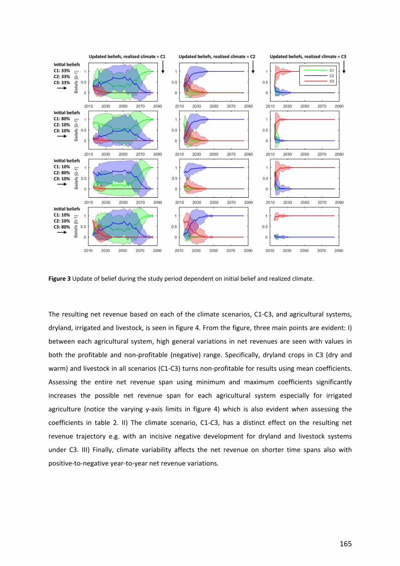
165  

 

 

Figure 3 Update of belief during the study period dependent on initial belief and realized climate.  

 

The resulting net revenue based on each of the climate scenarios, C1‐C3, and agricultural systems, 

dryland, irrigated and livestock, is seen in figure 4. From the figure, three main points are evident: I) 

between each agricultural system, high general variations  in net  revenues are seen with values  in 

both  the profitable and non‐profitable  (negative)  range. Specifically, dryland  crops  in C3  (dry and 

warm) and livestock in all scenarios (C1‐C3) turns non‐profitable for results using mean coefficients. 

Assessing  the  entire  net  revenue  span  using  minimum  and  maximum  coefficients  significantly 

increases  the  possible  net  revenue  span  for  each  agricultural  system  especially  for  irrigated 

agriculture  (notice  the  varying  y‐axis  limits  in  figure  4) which  is  also  evident when  assessing  the 

coefficients  in  table  2.  II)  The  climate  scenario,  C1‐C3,  has  a  distinct  effect  on  the  resulting  net 

revenue  trajectory  e.g. with  an  incisive  negative  development  for  dryland  and  livestock  systems 

under  C3.  III)  Finally,  climate  variability  affects  the  net  revenue  on  shorter  time  spans  also with 

positive‐to‐negative year‐to‐year net revenue variations.     

166  

 

 

Figure  4  Calculated  net  revenues  during  the  study  period  dependent  on  agricultural  system  practice  and realized climate. All results are plotted as minimum and maximum coefficients (95% confidence: coloured area – see  table 2) around  the mean net  revenue  functions  (Kurukulasuriya et al.  (2006). For easier comparison, results  are  sorted  for  both  agricultural  system  (left  column)  and  realized  climate  (right  column).  For  the realized climate, the y‐axis limits are specified to enable comparisons between dryland and livestock systems as the irrigated practice generates significantly higher net revenues.  

 

The  resulting  net  revenues  (USD/farm)  and  choice  of  agricultural  systems  (1‐3),  both  over  time 

(2020‐2085),  based  on  the  maximization  of  the  former,  is  shown  in  figure  5  using  mean  and 

minimum coefficients  for the combinations of the  four distributions of  initial beliefs and the three 

realised climates analysed. From figure 5 it is seen that employing irrigated agriculture is the optimal 

agricultural system regardless of the realised climate scenario when using mean coefficients. The net 

revenue  function  following  the  development  of  the  climate  trajectory,  for  C1  being  the  realised 

climate scenario, shows  large variation  in the net revenue  function when the decision maker have 

different  initial beliefs. The distance between  the curves also represent  the range of net revenues 

that the decision makers take decision upon, because of their  large variation  in  initial belief of the 

future climate development. When using minimum coefficients, dryland agriculture is preferred over 

the other agricultural systems  in 2025 and  from 2035 and onwards  for C1 and C2, whereas  for C3 

irrigated  agriculture  still  maximizes  net  revenue  (converged  from  2040  and  onwards).  For  all 

combinations of realised climate and coefficients, the influence of initial belief is seen to diminish or 

completely disappear within, most often, the first 5‐10 simulation years. Climate scenario C1, using 

167  

mean coefficients, is an exception. This is caused by the corresponding substantial shifts in belief for 

C1 throughout the analysis period as evident in figure 3.         

 

  

 

Figure 5 Choice of agricultural system (1‐3) based on net revenue maximization (USD/farm) dependent on the realized climate in the three climate scenarios (C1‐C3; temperature and precipitation) and the farmer's initial belief. Results are presented dependent on the use of mean or minimum (95% confidence) net revenue coefficients (table 2) as discussed above (as in Kurukulasuriyaet al. (2006)). 

  

   

168  

Concluding Discussion  

 

This  study presents a novel approach  to  simulate  the  consequence of decision making under  the 

impact  of  climate  changes,  simulating  how  a  decision  maker  can  change  behaviour  and  the 

consequence of the decisions as new knowledge  is revealed over time. The paper also adds to the 

discussion on how Bayesian updating can contribute  to  the development of adaptation  to climate 

change, and how the decision‐maker can handle the uncertainty of climate change. Therefore, the 

discussion  will  focus  on  the  Bayesian  updating  framework  developed  here,  its  relevance  and 

opportunities  for  improvement. The  results  regarding which agricultural  system  should be  chosen 

when and the possible net revenue will only be briefly touched upon, as the data and net revenue 

functions are judged too general; cf. the above section on Agricultural Systems. 

The  approach  helps  to  bridge  the  development  within  climate  change  and  the  management 

decisions  facing  farmers. The  latter  is often based on a combination of variables, e.g. sociological, 

economic  and  ecological.  This  paper  solely  considers  the  farmer’s  observation  of  the  climate 

variables  precipitation  and  temperature,  updating  his  belief  of  the  true  climate  development, 

followed by an observation of net  revenue  from  the agriculture  system based on his belief  in  the 

climate, and a decision based on these observations. Despite this limitation, the approach presented 

here  is useful  in that  it frames the different options available to farmers facing climate change and 

the consequence of having a misjudged initial belief.  

The main  finding of  this paper  is  that with  the method presented,  it  is possible  to simulate  future 

choices of the farmer, to contradict original beliefs and to highlight the consequences it can have to 

make  a wrong  choice. A  key  finding  is  that  irrigated  crops,  independently of  the  realised  climate 

development, is a main preferred choice of agricultural system due to the, upward‐sloping curve for 

net  revenue  (US  dollars  per  farm/year)    regardless  of  climate  scenario  (figure  3).  The  choice  of 

irrigated crops may, however, be too optimistic and unrealistic; as the  implementation of  irrigated 

crops will require making considerable  investments (depending on the way  irrigation  is established 

and  carried  out).  Irrigated  crops may be unrealistic  for many  farmers,  as  this  agricultural  system 

entails more intensive management, high costs for implementation and the system is therefore not 

necessarily available  to  the majority of  farmers. Further,  the mean  coefficients used  (table 2) are 

likely to be affected by, and therefore biased towards, countries where irrigation water available and 

therefore implemented into the agricultural system, here mainly Egypt Kurukulasuriya et al. (2006). 

Therefore,  the  results based on using  the minimum coefficients  (95% confidence), where also  the 

169  

dryland agricultural system  is preferred  for  two climate scenarios,  is  likely  to be more  realistic  for 

this Ghanaian example. The  right  column  in  figure 4  shows how  the agricultural  system becomes 

competitive with one another and the development through the three climate scenarios and time. 

By  applying  the minimum  coefficients  it  has  been  possible  to  show  how  the  decision‐maker  can 

change behaviour over time, as new  information  is revealed, contradicting his original beliefs. This 

proves  that  it  is possible  to  simulate a  change  in a  reaction patterns among  farmers  in examples 

where the climate does not develop as predicted and according to the farmers belief.  

The lack of opportunities to implementing irrigated farming, as highlighted above, also has another 

implication  regarding  the  remaining  two agricultural  systems. Dryland  crops are  cultivated on  the 

farmer’s privately owned land, whereas it is normal in many locations to use common or public land 

for livestock grazing (Kurukulasuriya et al. 2006; Kassahun and Jacobsen 2015). Consequently, there 

is no linear relationship between a farmer’s income from livestock and the amount of land he owns 

or has the right to cultivate. The choice between livestock and dryland crops is thus more a matter of 

where  to make an effort  in  terms of  required  investments  (e.g.  seeds, animals) and  labour. Also, 

livestock  covers  a  huge  range  of  animals,  and  it  should  be  taken  into  consideration  that  small 

livestock  such  as  goats  are  more  heat  tolerant  than  cattle.  This  has  to  some  extent  been 

incorporated into the net revenue for livestock, as the data from Kurukulasuriya et al. (2006) include 

a variety of contributions and alternative actions, which farmers have  introduced  in order to adapt 

to  current  climate  viabilities. The discussion  concerning where  to make  the effort  also  leads  to  a 

discussion  of  the  cost  of  labour,  as  the  cost  of  household  labour  has  not  been  included  in  the 

functions for the net revenue of the different agricultural systems. The results of Kurukulasuriya et 

al.  (2006)  indicate  that  growing  crops  is  more  management  intensive  than  keeping  livestock. 

Kurukulasuriya et al.  (2006) base  this assumption on  the  fact  that a  large household earns higher 

revenue from crops and lower revenue from livestock than smaller households. The function applied 

in figure 4 based on Kurukulasuriya et al. (2006) clearly shows that the net revenue generated from 

livestock are more sensitive  to climate change variabilities,  than dryland crops exemplified  though 

the large variabilities in the net revenue functions for irrigated crops compare to dryland crops. This 

then  indicates  that  the  farmer  is  likely  to be more willing  to update his beliefs  if changes concern 

precipitation  rather  than  temperature,  as  precipitation  has  a  greater  influence  on  growth.  The 

decision‐maker  may  erroneously  update  his  beliefs  on  precipitation,  as  there  can  be  huge 

fluctuations  in  precipitation.  And  further;  the  decision‐makers  (should)  therefore  require  a  solid 

knowledge base for updating his beliefs in a realistic way. This could be the explanation on why we 

see the frequent change among agriculture systems in figure 5, among for calculations on minimum 

coefficients  in  the  early  years  until  year  2040.  The  increasing  precipitation  patterns  for  C2  from 

170  

approx. 2040 and onwards causes the  farmer to choose dryland crops  from this point  in time. For 

the C3  scenario,  the decrease  in precipitation  causes  the opposite  towards  a  choice  for  irrigated 

crops. Some effect may further be seen for the stronger temperature increase for C3 over C2 (figure 

1).  

With regard to farmers’ ability to react in a proactive way in order to adapt to climate changes, we 

have considered  it  relevant  to compare  the  three agricultural systems within  this  framework, as a 

change  in  agricultural  system  is  at  some  level  an  irreversible  decision  towards  being  resilient  to 

climate change for the current period (5 years), compared to more untenable coping strategies such 

as reduced consumption, cash savings or  increase  in debt. However, we should not forget that the 

setting  is  highly  dynamic,  and  as  highlighted  above,  the  line  between  proactive  and  reactive 

behaviour can be blurred, meaning that what  is optimal today may not be optimal next year. One 

should  also  pay  attention  to  the  findings  of  Antwi‐Agyei, Dougill  and  Stringer  (2015)  concerning 

barriers to climate change adaptation: It can be difficult for the individual farmer to sell his crops if 

there is no market; this is a question of supply and demand and having access to a market – a barrier 

which not even this framework can overcome.   

Furthermore,  it may be relevant  to mention how most  farmers will  in  fact choose  to combine  the 

three  suggested  agricultural  systems.  Kurukulasuriya  et  al.  (2006)  also  mentioned  this  in  their 

description of  the data, assuming  that  the  farmer chooses  input and output  that optimise  the net 

revenue  of  these  three main  agricultural  systems  and minimise  the  risk,  something  the  current 

framework was not able to handle. 

The  approach  presented  here  helps  in  bridging  the  development within  climate  change  and  the 

management decisions farmers are facing. The latter in integrated decision support systems is often 

based on a combination of variables, e.g. sociological, economic and ecological. This paper focuses 

on  the  farmer’s observation of  the  climate  variables precipitation  and  temperature, updating  his 

belief  of  the  true  climate  development,  followed  by  an  observation  of  net  revenue  from  the 

agriculture system based on a belief in the climate, and a decision based on these observations. This 

may somewhat prove to be a  limitation of the approach although  facilitating the different options 

available to farmers facing climate change.  

In the approach presented here, we aim at applying a more thorough analysis and  implementation 

of the climate data component of this type of study. This, not only by applying the most recent set of 

regional  climate model  simulations available but also by  integrating  these  in a  fashion where not 

only the extreme end‐period outcomes are included (e.g. high temperature increases by 2100), but 

171  

also by analysing and  including much diverging  trajectories of both  temperature and precipitation 

and  the associated  correlations and variabilities. We  thereby enable  the assessment of a broader 

range  of  the  possible  span  of  resulting  outcomes  in  net  revenues  and  associated  agricultural 

decision‐making.  

The Bayesian updating  framework  is a  first  step  in developing a  theoretical approach  to updating 

beliefs  on  climate  change,  making  proactive  adaptation  possible,  whether  being  proactive  or 

reactive. Most  importantly however, we recognise the need to move from the current farm‐based 

level  of  advancement  to  working  in  a  village  or  country  setting,  when  the  issue  is  scarcity  of 

resources,  e.g. water,  as  it will  not  be  possible  for  all  farmers  to  irrigate  their  crops  under  the 

influence  of  climate  change,  even  if  the  results  of  the  Bayesian  framework  suggest  that  this 

agricultural  system  is  preferable.  Of  other  settings where  this  approach  could  be  relevant  is  in 

relation to the implementation of policies, decision support for a region or support from donors and 

NGO's, as this is often very time consuming to implement and can have similarities with irreversible 

decisions. 

Future research on this matter should focus on the possibility of merging individual decision‐making 

with available resources, based on more empirical knowledge of farmer's choice of climate change 

adaptation  or  coping  in  the  case  of  substantial  unexpected  shocks.  A more  specific  analysis  on 

sustainability aspects and consequences of decisions under a given climate change scenario should 

therefore be possible also highlighting  resilience.  In a wider perspective  it would be  interesting  to 

see  how  a  Bayesian  framework  could  contribute  to  revealing  and  identifying  opportunities  for 

adaptation and mitigation of climate changes and – if possible – how it may contribute to optimising 

farmers’ resilience to climate change and increased sustainable development. 

 

Acknowledgements 

 

Jette Bredahl Jacobsen, Anne Olhoff and colleagues at UNEP DTU partnership (UDP) are thanked for 

providing constructive criticism and feedback and Rasoul Yousefpour for giving the originally 

inspiration. 

    

172  

References   Antwi‐Agyei P, Dougill AJ, Stringer LC (2015) Barriers to climate change adaptation: evidence 

from northeast Ghana in the context of a systematic literature review. Climate and Development 7:297–309. doi: 10.1080/17565529.2014.951013 

Antwi‐Agyei P, Fraser EDG, Dougill AJ, et al (2012) Mapping the vulnerability of crop production to drought in Ghana using rainfall, yield and socioeconomic data. Applied Geography 32:324–334. doi: 10.1016/j.apgeog.2011.06.010 

Antwi‐Agyei P, Stringer LC, Dougill AJ (2014) Livelihood adaptations to climate variability: insights from farming households in Ghana. Regional Environmental Change 14:1615–1626. doi: 10.1007/s10113‐014‐0597‐9 

Arrow KJ, Fisher AC (1974) Environmental Preservation, Uncertainty and Irreversibility. Quarterly Journal of Economics 88:312‐319. 

Baldauf M, Seifert A, Förstner J, et al (2011) Operational Convective‐Scale Numerical Weather Prediction with the COSMO Model: Description and Sensitivities. Monthly Weather Review 139:3887–3905. doi: 10.1175/MWR‐D‐10‐05013.1 

Bayes T, Price M (1763) An Essay towards Solving a Problem in the Doctrine of Chances. Philosophical Transactions of the Royal Society of London. 53:370‐418. 

Benhin JKA (2008) South African crop farming and climate change: An economic assessment of impacts. Global Environmental Change 18:666–678. doi: 10.1016/j.gloenvcha.2008.06.003 

Berg P, Döscher R, Koenigk T (2013) Impacts of using spectral nudging on regional climate model RCA4 simulations of the Arctic. Geoscientific Model Development Discussions 6:495–520. doi: 10.5194/gmdd‐6‐495‐2013 

Boko M, Niang I, Nyong A, et al (2007) Africa. In: Climate Change 2007: Impacts, Adaptation and Vulnerability. Contribution of Working Group II to the Fourth Assessment Report of the Intergovernmental Panel on Climate Change. M. L. Parry, O. F. Canziani, J. P. Palutikof, P. J. van der Linden and C. E. Hanson (Eds.). Cambridge University Press, Cambridge, UK, pp. 433‐467. 

Christensen OB, Drews M, Hesselbjerg JC, et al (2007) The HIRHAM Regional Climate Model. Version 5 (beta). Danish Climate Centre, Danish Meteorological Institute 

Budescu DV, Broomell S, Por H‐H (2009) Improving communication of uncertainty in the reports of the Intergovernmental Panel on Climate Change. Psychological science 20:299–308. 

Challinor AJ, Watson J, Lobell DB, et al (2014) A meta‐analysis of crop yield under climate change and adaptation. Nature Climate Change 4:287–291. doi: 10.1038/nclimate2153 

Das Gupta M (2014) Population, Poverty, and Climate Change. World Bank Research Observer 29, No. 1: 83‐108. 

Deser C, Phillips A, Bourdette V, Teng H (2012) Uncertainty in climate change projections: the role of internal variability. Clim Dyn 38:527–546. doi: 10.1007/s00382‐010‐0977‐x 

Déqué M, Calmanti S, Christensen OB, et al (2016) A multi‐model climate response over tropical Africa at +2°C. Climate Services. doi: 10.1016/j.cliser.2016.06.002 

Field CB, Barros VR, Mastrandrea MD, et al (2014) Summary for policymakers. Climate change 2014: impacts, adaptation, and vulnerability Part A: global and sectoral aspects Contribution of Working Group II to the Fifth Assessment Report of the Intergovernmental Panel on Climate Change 1–32. 

173  

Frankhauser S, Smith JB, Tol RSJ (1999) Weathering climate change: some simple rules to guide adaptation decisions. Ecological Economics 30(1):67‐78. 

Halsnæs K, Shukla P, Ahuja D, et al (2007) Framing issues. In: Climate Change 2007: Mitigation. Contribution of Working Group III to the Fourth Assessment Report of the Intergovernmental Panel on Climate Change. Metz, B., Davidson, O. R., Bosch, P. R., Dave, R. and Meyer, L. A. (Eds.). Cambridge University Press, Cambridge, UK and New York, NY, USA, pp. 117‐167. 

Hawkins E, Sutton R (2011) The potential to narrow uncertainty in projections of regional precipitation change. Climate Dynamics 37:407–418. doi: 10.1007/s00382‐010‐0810‐6 

IPCC (2013) Climate Change 2013: The Physical Science Basis. Contribution of Working Group I to the Fifth Assessment Report of the Intergovernmental Panel on Climate Change. Stocker TF, Qin D, Plattner G‐K, et al (Eds.). Cambridge University Press, Cambridge, UK and New York, NY, USA. 

IPCC (2014) Summary for policymakers. In: Climate Change 2014: Impacts, Adaptation, and Vulnerability. Part A: Global and Sectoral Aspects. Contribution of Working Group II to the Fifth Assessment Report of the Intergovernmental Panel on Climate Change. Field CB, Barros VR, Dokken DJ, et al (Eds.). Cambridge University Press, Cambridge, United Kingdom and New York, NY, USA. 

Jacob D, Elizalde A, Haensler A, et al (2012) Assessing the Transferability of the Regional Climate Model REMO to Different COordinated Regional Climate Downscaling EXperiment (CORDEX) Regions. Atmosphere 3:181–199. doi: 10.3390/atmos3010181 

Kassahun HT, Jacobsen JB (2015) Economic and institutional incentives for managing the Ethiopian highlands of the Upper Blue Nile Basin: A latent class analysis. Land Use Policy 44:76–89. doi: 10.1016/j.landusepol.2014.11.017 

Klibanoff P, Marinacci M, Mukerji S (2005) A smooth model of decision making under ambiguity. Econometrica 73:1849–1892. 

Kurukulasuriya P (2006) Will African Agriculture Survive Climate Change? The World Bank Economic Review 20:367–388. doi: 10.1093/wber/lhl004 

Larsen MAD, Thejll P, Christensen JH, et al (2013) On the role of domain size and resolution in the simulations with the HIRHAM region climate model. Climate Dynamics 40:2903–2918. doi: 10.1007/s00382‐012‐1513‐y 

Lecocq F, Shalizi Z (2007) Balancing expenditures on mitigation of and adaptation to climate change: an exploration of issues relevant to developing countries.  

Nikulin G, Jones C, Giorgi F, et al (2012) Precipitation Climatology in an Ensemble of CORDEX‐Africa Regional Climate Simulations. Journal of Climate 25:6057–6078. doi: 10.1175/JCLI‐D‐11‐00375.1 

Oreskes N, Shrader‐Frechette K, Belitz, K (1994) Verification, Validation, and Confirmation of Numerical Models in the Earth Sciences. Science 263:641‐646. 

Refsgaard JC, Madsen H, Andréassian V, et al (2014) A framework for testing the ability of models to project climate change and its impacts. Climatic Change 122:271–282. doi: 10.1007/s10584‐013‐0990‐2 

Simal PD, Ortega ST (2011) Option and quasi‐option value. An approach to deal with climate change effects in coastal areas. Oceans, 2011 IEEE – Spain, pp. 1‐7. 

Stern N (2006) The Economist of Climate Change: The Stern Review. Cambridge University Press, Cambridge, UK and New York, NY, USA. 

174  

Stocker TF, Qin D, Plattner GK, et al (2013) IPCC, 2013: climate change 2013: the physical science basis. Contribution of working group I to the fifth assessment report of the intergovernmental panel on climate change.  

Tschakert P, Dietrich KA, others (2010) Anticipatory learning for climate change adaptation and resilience. Ecology and society 15:11. 

Van Meijgaard E, Van Ulft LH, Van de Berg WJ, et al (2008) The KNMI regional atmospheric climate model RACMO version 2.1.  

Vardas G, Xepapadeas A (2010) Model Uncertainty, Ambiguity and the Precautionary Principle: Implications for Biodiversity Management. Environmental and Resource Economics 45:379–404. doi: 10.1007/s10640‐009‐9319‐z 

Yip S, Ferro CAT, Stephenson DB, Hawkins E (2011) A Simple, Coherent Framework for Partitioning Uncertainty in Climate Predictions. Journal of Climate 24:4634–4643. doi: 10.1175/2011JCLI4085.1 

Yousefpour R, Didion M, Jacobsen JB, et al (2015) Modelling of adaptation to climate change and decision‐makers behaviours for the Veluwe forest area in the Netherlands. Forest Policy and Economics 54:1–10. doi: 10.1016/j.forpol.2015.02.002 

Yousefpour R, Jacobsen JB, Meilby H, Thorsen BJ (2014) Knowledge update in adaptive management of forest resources under climate change: a Bayesian simulation approach. Annals of Forest Science 71:301–312. doi: 10.1007/s13595‐013‐0320‐x 

Zadra A, Caya D, Côté J, et al (2008) The next Canadian regional climate model. Phys Can 64:75–83.