1596932341 intercept radar.pdf
TRANSCRIPT

7/17/2019 1596932341 Intercept Radar.pdf
http://slidepdf.com/reader/full/1596932341-intercept-radarpdf 1/891

7/17/2019 1596932341 Intercept Radar.pdf
http://slidepdf.com/reader/full/1596932341-intercept-radarpdf 2/891
Detecting and ClassifyingLow Probability of Intercept Radar
Second Edition

7/17/2019 1596932341 Intercept Radar.pdf
http://slidepdf.com/reader/full/1596932341-intercept-radarpdf 3/891
For a listing of recent titles in the Artech House Radar Library ,turn to the back of this book.
DISCLAIMEROFWARRANTY
The technical descriptions, procedures, and computer programs in this book have been developed with the greatest of care and they have been useful to theauthor in a broad range of applications; however, they are provided as is, with-out warranty of any kind. Artech House, Inc. and the author and editors of thebook titled Detecting and Classifying Low Probability of Intercept Radar, Second Edition make no warranties, expressed or implied, that the equations, programs,and procedures in this book or its associated software are free of error, or are
consistent with any particular standard of merchantability, or will meet yourrequirements for any particular application. They should not be relied upon forsolving a problem whose incorrect solution could result in injury to a person orloss of property. Any use of the programs or procedures in such a manner is atthe user’s own risk. The editors, author, and publisher disclaim all liability fordirect, incidental, or consequent damages resulting from use of the programs orprocedures in this book or the associated software.

7/17/2019 1596932341 Intercept Radar.pdf
http://slidepdf.com/reader/full/1596932341-intercept-radarpdf 4/891
Detecting and ClassifyingLow Probability of Intercept Radar
Second Edition
Phillip E. Pace

7/17/2019 1596932341 Intercept Radar.pdf
http://slidepdf.com/reader/full/1596932341-intercept-radarpdf 5/891
Library of Congress Cataloging-in-Publication Data A catalog record for this book is available from the Library of Congress.
British Library Cataloguing in Publication Data A catalogue record for this book is available from the British Library.
ISBN-13 978-1-59693-234-0
Cover design by Igor Valdman
© 2009 ARTECH HOUSE685 Canton Street Norwood, MA 02062
All rights reserved. Printed and bound in the United States of America. No part of this book may be reproduced or utilized in any form or by any means, electronic or mechanical, including pho-tocopying, recording, or by any information storage and retrieval system, without permission in
writing from the publisher. All terms mentioned in this book that are known to be trademarks orservice marks have been appropriately capitalized. Artech House cannot attest to the accuracy of this information. Use of a term in this book should not be regarded as affecting the validity of any trademark or service mark.
10 9 8 7 6 5 4 3 2 1
Disclaimer:
This eBook does not include the ancil lary media that was
packaged with the or iginal printed version of the book.

7/17/2019 1596932341 Intercept Radar.pdf
http://slidepdf.com/reader/full/1596932341-intercept-radarpdf 6/891
To my wif e,
Ann Marie Pace,
and
to our chi ldren,
Amanda, Zachary, and Molly

7/17/2019 1596932341 Intercept Radar.pdf
http://slidepdf.com/reader/full/1596932341-intercept-radarpdf 7/891
7/17/2019 1596932341 Intercept Radar.pdf
http://slidepdf.com/reader/full/1596932341-intercept-radarpdf 8/891
Contents
Foreword xix
Preface xxi
Acknowledgments xxix
PART I: FUNDAMENTALS OF LPI RADAR DESIGN 1
1 To See and Not Be Seen 3
1.1 The Requirement for LPI . . . . . . . . . . . . . . . . . . . . 31.2 Characteristics of LPI Radar . . . . . . . . . . . . . . . . . . 5
1.2.1 Antenna Considerations . . . . . . . . . . . . . . . . . 51.2.2 Achieving Ultra-Low Side Lobes . . . . . . . . . . . . 71.2.3 Antenna Scan Patterns for Search Processing . . . . . 101.2.4 Advanced Multifunction RF Concept . . . . . . . . . . 131.2.5 Transmitter Considerations . . . . . . . . . . . . . . . 141.2.6 Power Management . . . . . . . . . . . . . . . . . . . 161.2.7 Carrier Frequency Considerations . . . . . . . . . . . . 17
1.3 Pulse Compression—The Key to LPI Radar . . . . . . . . . . 18
1.4 Radar Detection Range . . . . . . . . . . . . . . . . . . . . . 241.5 Interception Range . . . . . . . . . . . . . . . . . . . . . . . . 271.6 Comparing Radar Range and Interception Range . . . . . . . 291.7 The Pilot LPI Radar . . . . . . . . . . . . . . . . . . . . . . . 311.8 Concluding Remarks . . . . . . . . . . . . . . . . . . . . . . . 36
References . . . . . . . . . . . . . . . . . . . . . . . . . . . . . 37Problems . . . . . . . . . . . . . . . . . . . . . . . . . . . . . 39
2 LPI Technology and Applications 41
2.1 Altimeters . . . . . . . . . . . . . . . . . . . . . . . . . . . . . 412.1.1 Introduction . . . . . . . . . . . . . . . . . . . . . . . 412.1.2 Fielded LPI Altimeters . . . . . . . . . . . . . . . . . 42
2.2 Landing Systems . . . . . . . . . . . . . . . . . . . . . . . . . 45
2.2.1 Introduction . . . . . . . . . . . . . . . . . . . . . . . 45
vii
7/17/2019 1596932341 Intercept Radar.pdf
http://slidepdf.com/reader/full/1596932341-intercept-radarpdf 9/891
viii Detecting and Classifying LPI Radar
2.2.2 Fielded LPI Landing Systems . . . . . . . . . . . . . . 462.3 Surveillance and Fire Control Radar . . . . . . . . . . . . . . 48
2.3.1 Battlefield Awareness . . . . . . . . . . . . . . . . . . 482.3.2 LPI Ground-Based Systems . . . . . . . . . . . . . . . 482.3.3 LPI Airborne Systems . . . . . . . . . . . . . . . . . . 56
2.4 Antiship Capable Missile and Torpedo Seekers . . . . . . . . 582.4.1 A Significant Threat to Surface Navies . . . . . . . . . 582.4.2 Fielded LPI Seeker Systems . . . . . . . . . . . . . . . 58
2.5 Summary of LPI Radar Systems . . . . . . . . . . . . . . . . 62References . . . . . . . . . . . . . . . . . . . . . . . . . . . . . 64Problems . . . . . . . . . . . . . . . . . . . . . . . . . . . . . 65
3 Ambiguity Analysis of LPI Waveforms 67
3.1 The Ambiguity Function . . . . . . . . . . . . . . . . . . . . . 683.2 Periodic Autocorrelation Function . . . . . . . . . . . . . . . 683.3 Periodic Ambiguity Function . . . . . . . . . . . . . . . . . . 69
3.3.1 Periodicity of the PAF . . . . . . . . . . . . . . . . . . 703.3.2 Peak and Integrated Side Lobe Levels . . . . . . . . . 70
3.4 Frank Phase Modulation Example . . . . . . . . . . . . . . . 713.4.1 Transmitted Waveform . . . . . . . . . . . . . . . . . . 713.4.2 Simulation Results . . . . . . . . . . . . . . . . . . . . 72
3.5 Reducing the Doppler Side Lobes . . . . . . . . . . . . . . . . 75References . . . . . . . . . . . . . . . . . . . . . . . . . . . . . 78Problems . . . . . . . . . . . . . . . . . . . . . . . . . . . . . 78
4 FMCW Radar 81
4.1 Advantages of FMCW . . . . . . . . . . . . . . . . . . . . . . 814.2 Single Antenna LPI Radar for Target Detection . . . . . . . . 83
4.3 Transmitted Waveform Design . . . . . . . . . . . . . . . . . 864.3.1 Triangular Waveform . . . . . . . . . . . . . . . . . . . 864.3.2 Waveform Spectrum . . . . . . . . . . . . . . . . . . . 894.3.3 Generating Linear FM Waveforms . . . . . . . . . . . 91
4.4 Receiver-Transmitter Isolation . . . . . . . . . . . . . . . . . 944.4.1 Transmission Line Basics . . . . . . . . . . . . . . . . 954.4.2 Single Antenna Isolation Using a Circulator . . . . . . 964.4.3 Single Antenna Isolation Using a Reflected Power
Canceler . . . . . . . . . . . . . . . . . . . . . . . . . . 974.5 The Received Signal . . . . . . . . . . . . . . . . . . . . . . . 1004.6 LPI Search Mode Processing . . . . . . . . . . . . . . . . . . 1014.7 Track Mode Processing Techniques . . . . . . . . . . . . . . . 1044.8 Eff ect of Sweep Nonlinearities . . . . . . . . . . . . . . . . . . 105
4.9 Moving Target Indication Filtering . . . . . . . . . . . . . . . 1074.10 Matched Receiver Response . . . . . . . . . . . . . . . . . . . 1084.11 Mismatched Receiver Response . . . . . . . . . . . . . . . . . 110

7/17/2019 1596932341 Intercept Radar.pdf
http://slidepdf.com/reader/full/1596932341-intercept-radarpdf 10/891
Table of Contents ix
4.12 PANDORA FMCW Radar . . . . . . . . . . . . . . . . . . . 1134.13 Electronic Attack Considerations . . . . . . . . . . . . . . . . 1154.14 Technology Trends for FMCW Emitters . . . . . . . . . . . . 115
References . . . . . . . . . . . . . . . . . . . . . . . . . . . . . 119Problems . . . . . . . . . . . . . . . . . . . . . . . . . . . . . 122
5 Phase Shift Keying Techniques 125
5.1 Introduction . . . . . . . . . . . . . . . . . . . . . . . . . . . . 1255.2 The Transmitted Signal . . . . . . . . . . . . . . . . . . . . . 1265.3 Binary Phase Codes . . . . . . . . . . . . . . . . . . . . . . . 1285.4 Polyphase Codes . . . . . . . . . . . . . . . . . . . . . . . . . 1335.5 Polyphase Barker Codes . . . . . . . . . . . . . . . . . . . . . 1345.6 Frank Code . . . . . . . . . . . . . . . . . . . . . . . . . . . . 1395.7 P1 Code . . . . . . . . . . . . . . . . . . . . . . . . . . . . . . 1485.8 P2 Code . . . . . . . . . . . . . . . . . . . . . . . . . . . . . . 1525.9 P3 Code . . . . . . . . . . . . . . . . . . . . . . . . . . . . . . 1525.10 P4 Code . . . . . . . . . . . . . . . . . . . . . . . . . . . . . . 1575.11 P olytime Codes . . . . . . . . . . . . . . . . . . . . . . . . . . 163
5.11.1 T1(n) Code . . . . . . . . . . . . . . . . . . . . . . . . 1635.11.2 T2(n) Code . . . . . . . . . . . . . . . . . . . . . . . . 1655.11.3 T3(n) Code . . . . . . . . . . . . . . . . . . . . . . . . 1695.11.4 T4(n) Code . . . . . . . . . . . . . . . . . . . . . . . . 169
5.12 Omnidirectional LPI Radar . . . . . . . . . . . . . . . . . . . 1795.13 Summary . . . . . . . . . . . . . . . . . . . . . . . . . . . . . 182
References . . . . . . . . . . . . . . . . . . . . . . . . . . . . . 182Problems . . . . . . . . . . . . . . . . . . . . . . . . . . . . . 183
6 Frequency Shift Keying Techniques 187
6.1 Advantages of the FSK Radar . . . . . . . . . . . . . . . . . . 1876.2 Description of the FSK CW Signal . . . . . . . . . . . . . . . 1896.3 Range Computation in FSK Radar . . . . . . . . . . . . . . . 1896.4 Costas Codes . . . . . . . . . . . . . . . . . . . . . . . . . . . 191
6.4.1 Characteristics of a Costas Array or Sequence . . . . . 1916.4.2 Computing the Diff erence Triangle . . . . . . . . . . . 1926.4.3 Deriving the Costas Sequence PAF . . . . . . . . . . . 1926.4.4 Welch Construction of Costas Arrays . . . . . . . . . . 193
6.5 Hybrid FSK/PSK Technique . . . . . . . . . . . . . . . . . . 1956.5.1 Description of the FSK/PSK Signal . . . . . . . . . . 195
6.6 Matched FSK/PSK Signaling . . . . . . . . . . . . . . . . . . 1996.7 Concluding Remarks . . . . . . . . . . . . . . . . . . . . . . . 201
References . . . . . . . . . . . . . . . . . . . . . . . . . . . . . 205
Problems . . . . . . . . . . . . . . . . . . . . . . . . . . . . . 206

7/17/2019 1596932341 Intercept Radar.pdf
http://slidepdf.com/reader/full/1596932341-intercept-radarpdf 11/891
x Detecting and Classifying LPI Radar
7 Noise Techniques 207
7.1 Historical Perspective . . . . . . . . . . . . . . . . . . . . . . 2077.2 Ultrawideband Considerations . . . . . . . . . . . . . . . . . . 2107.3 Principles of Random Noise Radars . . . . . . . . . . . . . . . 2127.4 Narayanan Random Noise Radar Design . . . . . . . . . . . . 215
7.4.1 Operating Characteristics . . . . . . . . . . . . . . . . 2167.4.2 Model of RNR Transmitter . . . . . . . . . . . . . . . 2197.4.3 Periodic Ambiguity Results . . . . . . . . . . . . . . . 219
7.5 Random Noise Plus FMCW Radar . . . . . . . . . . . . . . . 2227.5.1 RNFR Spectrum . . . . . . . . . . . . . . . . . . . . . 2237.5.2 Model of RNFR Transmitter . . . . . . . . . . . . . . 2257.5.3 Periodic Ambiguity Results . . . . . . . . . . . . . . . 225
7.6 Random Noise FMCW Plus Sine . . . . . . . . . . . . . . . . 2277.6.1 Model of RNFSR Transmitter . . . . . . . . . . . . . . 2297.6.2 Periodic Ambiguity Results . . . . . . . . . . . . . . . 230
7.7 Random Binary Phase Modulation . . . . . . . . . . . . . . . 2347.7.1 Model of RBPC Transmitter . . . . . . . . . . . . . . 2367.7.2 Periodic Ambiguity Results . . . . . . . . . . . . . . . 236
7.8 Millimeter Wave Noise Radar . . . . . . . . . . . . . . . . . . 2387.9 Correlation Receiver Techniques . . . . . . . . . . . . . . . . 238
7.9.1 Ideal Correlation . . . . . . . . . . . . . . . . . . . . . 2397.9.2 Digital-Analog Correlation . . . . . . . . . . . . . . . 2397.9.3 Fully Digital Correlation . . . . . . . . . . . . . . . . . 2417.9.4 Acousto-Optic Correlation . . . . . . . . . . . . . . . . 242
7.10 Concluding Remarks . . . . . . . . . . . . . . . . . . . . . . . 243References . . . . . . . . . . . . . . . . . . . . . . . . . . . . . 244Problems . . . . . . . . . . . . . . . . . . . . . . . . . . . . . 247
8 Over-the-Horizon Radar 2498.1 Two Types of OTHR . . . . . . . . . . . . . . . . . . . . . . . 2498.2 Sky Wave OTHR . . . . . . . . . . . . . . . . . . . . . . . . . 252
8.2.1 Characteristics of the Ionosphere . . . . . . . . . . . . 2538.2.2 Example of F2-Layer Propagation . . . . . . . . . . . 2598.2.3 Doppler Clutter Spectrum . . . . . . . . . . . . . . . . 2598.2.4 Example Sky Wave OTHR System . . . . . . . . . . . 2618.2.5 Sky Wave Processing . . . . . . . . . . . . . . . . . . . 261
8.3 Sky Wave LPI Waveform Considerations . . . . . . . . . . . . 2658.3.1 Phase Modulation Techniques . . . . . . . . . . . . . . 2658.3.2 Costas Frequency Hopping . . . . . . . . . . . . . . . 2668.3.3 Reducing the CIT . . . . . . . . . . . . . . . . . . . . 2668.3.4 Multiple Waveform Repetition Frequencies . . . . . . 266
8.3.5 Out-of-Band Emission Suppression . . . . . . . . . . . 2708.4 Sky Wave Maximum Detection Range . . . . . . . . . . . . . 2718.5 Sky Wave Footprint Prediction . . . . . . . . . . . . . . . . . 274

7/17/2019 1596932341 Intercept Radar.pdf
http://slidepdf.com/reader/full/1596932341-intercept-radarpdf 12/891
Table of Contents xi
8.6 Surface Wave OTHR . . . . . . . . . . . . . . . . . . . . . . . 2768.6.1 Example Surface Wave OTHR System . . . . . . . . . 281
8.7 Surface Wave LPI Waveform Considerations . . . . . . . . . . 2828.7.1 FMICW Characteristics . . . . . . . . . . . . . . . . . 2828.7.2 FMICW Ambiguity Space . . . . . . . . . . . . . . . . 287
8.8 Surface Wave Maximum Detection Range . . . . . . . . . . . 2888.9 Concluding Remarks . . . . . . . . . . . . . . . . . . . . . . . 295
References . . . . . . . . . . . . . . . . . . . . . . . . . . . . . 295Problems . . . . . . . . . . . . . . . . . . . . . . . . . . . . . 299
9 Case Study: Antiship LPI Missile Seeker 301
9.1 History of ASCM Seeker Technology . . . . . . . . . . . . . . 3019.2 The Future for ASCM Technology . . . . . . . . . . . . . . . 3029.3 Detecting the Threat . . . . . . . . . . . . . . . . . . . . . . . 3059.4 ASCM Target Scenario . . . . . . . . . . . . . . . . . . . . . . 306
9.4.1 Low RCS Targets . . . . . . . . . . . . . . . . . . . . . 3069.4.2 Sea Clutter Model . . . . . . . . . . . . . . . . . . . . 3089.4.3 Linear FMCW Emitter Power Management . . . . . 3109.4.4 Target-to-Clutter Ratio . . . . . . . . . . . . . . . . . 312
9.5 ASCM Ship Target Model . . . . . . . . . . . . . . . . . . . . 315References . . . . . . . . . . . . . . . . . . . . . . . . . . . . . 315Problems . . . . . . . . . . . . . . . . . . . . . . . . . . . . . 316
10 Network-Centric Warfare and Netted LPI Radar Systems 319
10.1 Network-Centric Warfare . . . . . . . . . . . . . . . . . . . . 31910.1.1 NCW Requirements . . . . . . . . . . . . . . . . . . . 32210.1.2 Situational Awareness . . . . . . . . . . . . . . . . . . 32310.1.3 Maneuverability . . . . . . . . . . . . . . . . . . . . . 323
10.1.4 Decision Speed and Operational Tempo . . . . . . . . 32410.1.5 Agility . . . . . . . . . . . . . . . . . . . . . . . . . . . 32510.1.6 Lethality . . . . . . . . . . . . . . . . . . . . . . . . . 326
10.2 Metrics for Information Grid Analysis . . . . . . . . . . . . . 32610.2.1 Generalized Connectivity Measure . . . . . . . . . . . 32610.2.2 Reference Connectivity Measure . . . . . . . . . . . . 32810.2.3 Network Reach . . . . . . . . . . . . . . . . . . . . . . 32910.2.4 Suppression Example . . . . . . . . . . . . . . . . . . 33110.2.5 Extended Generalized Connectivity Measure . . . . . 33310.2.6 Entropy and Network Richness . . . . . . . . . . . . . 33310.2.7 Maximum Operation Tempo . . . . . . . . . . . . . . 336
10.3 Electronic Attack . . . . . . . . . . . . . . . . . . . . . . . . . 33710.4 Information Network Analysis Using LPIsimNet . . . . . . . . 338
10.5 Netted LPI Radar Systems . . . . . . . . . . . . . . . . . . . 34210.5.1 Advantages of the Netted LPI Radar Systems . . . . . 34610.5.2 Netted LPI Radar Sensitivity . . . . . . . . . . . . . . 348

7/17/2019 1596932341 Intercept Radar.pdf
http://slidepdf.com/reader/full/1596932341-intercept-radarpdf 13/891
xii Detecting and Classifying LPI Radar
10.5.3 Signal Model . . . . . . . . . . . . . . . . . . . . . . . 34910.5.4 Netted Radar Electronic Attack . . . . . . . . . . . . 352
10.6 Netted Radar Analysis Using LPIsimNet . . . . . . . . . . . . 35310.6.1 Monostatic LPI Emitter and the SNR Contour Chart 35310.6.2 Three Netted LPI Emitters . . . . . . . . . . . . . . . 35410.6.3 Two Netted LPI Emitters with Jammer . . . . . . . . 358
10.7 Orthogonal Waveforms for Netted Radar . . . . . . . . . . . . 35810.7.1 Orthogonal Polyphase Codes . . . . . . . . . . . . . . 36210.7.2 Addressing Doppler Shift Degradation . . . . . . . . . 36510.7.3 Orthogonal Frequency Hopping Sequences . . . . . . . 37010.7.4 Noise Waveforms . . . . . . . . . . . . . . . . . . . . 374
10.8 Netted Over-the-Horizon Radar Systems . . . . . . . . . . . . 377References . . . . . . . . . . . . . . . . . . . . . . . . . . . . . 378Problems . . . . . . . . . . . . . . . . . . . . . . . . . . . . . 380
PART II: INTERCEPT RECEIVER STRATEGIES
AND SIGNAL PROCESSING 385
11 Strategies for Intercepting LPI Radar Signals 387
11.1 EW Intercept Receiver Techniques . . . . . . . . . . . . . . . 38711.1.1 Traditional Approach . . . . . . . . . . . . . . . . . . 38711.1.2 The Look-Through Problem . . . . . . . . . . . . . . . 38811.1.3 Modern Network-Centric Concepts Arriving . . . . . . 389
11.2 Detecting the LPI Radar with UAVs . . . . . . . . . . . . . . 39111.3 Noncooperative Intercept Receivers . . . . . . . . . . . . . . 392
11.3.1 Comparison of Classic Receiver Architecturesfor Detecting LPI Waveforms . . . . . . . . . . . . . . 392
11.3.2 Digital EW Receivers . . . . . . . . . . . . . . . . . . 396
11.3.3 Direct RF Sampling . . . . . . . . . . . . . . . . . . . 39811.4 Demodulation of the LPI Waveform . . . . . . . . . . . . . . 40011.5 EW Receiver Challenges . . . . . . . . . . . . . . . . . . . . . 40011.6 Concluding Remarks . . . . . . . . . . . . . . . . . . . . . . . 402
References . . . . . . . . . . . . . . . . . . . . . . . . . . . . . 403
12 Wigner-Ville Distribution Analysis of LPI Radar
Waveforms 405
12.1 Wigner-Ville Distribution . . . . . . . . . . . . . . . . . . . . 40612.1.1 Continuous WVD . . . . . . . . . . . . . . . . . . . . 40612.1.2 Example Calculation: Real Input Signal . . . . . . . . 40912.1.3 Example Calculation: Complex Input Signal . . . . . 41112.1.4 Two-Tone Input Signal Results . . . . . . . . . . . . . 414
12.2 F MCW Analysis . . . . . . . . . . . . . . . . . . . . . . . . . 41912.3 B PSK Analysis . . . . . . . . . . . . . . . . . . . . . . . . . . 42112.4 Polyphase Code Analysis . . . . . . . . . . . . . . . . . . . . 426

7/17/2019 1596932341 Intercept Radar.pdf
http://slidepdf.com/reader/full/1596932341-intercept-radarpdf 14/891
Table of Contents xiii
12.5 Polytime Code Analysis . . . . . . . . . . . . . . . . . . . . . 42912.6 Distinguishing Between Phase Codes . . . . . . . . . . . . . . 43112.7 FSK and FSK/PSK Analysis . . . . . . . . . . . . . . . . . . 43812.8 Summary . . . . . . . . . . . . . . . . . . . . . . . . . . . . . 438
References . . . . . . . . . . . . . . . . . . . . . . . . . . . . . 442Problems . . . . . . . . . . . . . . . . . . . . . . . . . . . . . 444
13 Choi-Williams Distribution Analysis of LPI Radar
Waveforms 445
13.1 Mathematical Development . . . . . . . . . . . . . . . . . . . 44613.2 LPI Signal Analysis . . . . . . . . . . . . . . . . . . . . . . . 448
13.2.1 FMCW Analysis . . . . . . . . . . . . . . . . . . . . . 44913.2.2 BPSK Analysis . . . . . . . . . . . . . . . . . . . . . . 44913.2.3 Polyphase Code Analysis . . . . . . . . . . . . . . . . 45513.2.4 Polytime Code Analysis . . . . . . . . . . . . . . . . . 45513.2.5 FSK and FSK/PSK Analysis . . . . . . . . . . . . . . 458
13.3 Summary . . . . . . . . . . . . . . . . . . . . . . . . . . . . . 458References . . . . . . . . . . . . . . . . . . . . . . . . . . . . . 464Problems . . . . . . . . . . . . . . . . . . . . . . . . . . . . . 464
14 LPI Radar Analysis Using Quadrature Mirror Filtering 467
14.1 Time-Frequency Wavelet Decomposition . . . . . . . . . . . . 46814.1.1 Basis Functions . . . . . . . . . . . . . . . . . . . . . . 46814.1.2 Short-Time Fourier Transform Decomposition . . . . . 46914.1.3 Wavelets and the Wavelet Transform . . . . . . . . . . 46914.1.4 Wavelet Filters . . . . . . . . . . . . . . . . . . . . . . 472
14.2 Discrete Two-Channel Quadrature Mirror Filter Bank . . . . 47414.3 Tree Structure to Filter the Lowpass Component . . . . . . . 476
14.4 Tree Structure to Filter the Highpass Component . . . . . . . 47714.5 QMFB Tree Receiver . . . . . . . . . . . . . . . . . . . . . . . 47814.6 Example Calculations . . . . . . . . . . . . . . . . . . . . . . 482
14.6.1 Complex Single-Tone Signal . . . . . . . . . . . . . . . 48214.6.2 Complex Two-Tone Signal . . . . . . . . . . . . . . . . 485
14.7 F MCW Analysis . . . . . . . . . . . . . . . . . . . . . . . . . 48714.8 B PSK Analysis . . . . . . . . . . . . . . . . . . . . . . . . . . 48914.9 Polyphase Code Analysis . . . . . . . . . . . . . . . . . . . . 49414.10 Polytime Code Analysis . . . . . . . . . . . . . . . . . . . . . 49514.11 Costas Frequency Hopping Analysis . . . . . . . . . . . . . . 49914.12 FSK/PSK Signal Analysis . . . . . . . . . . . . . . . . . . . 49914.13 Noise Waveform Analysis . . . . . . . . . . . . . . . . . . . . 49914.14 Summary . . . . . . . . . . . . . . . . . . . . . . . . . . . . . 506
References . . . . . . . . . . . . . . . . . . . . . . . . . . . . . 509Problems . . . . . . . . . . . . . . . . . . . . . . . . . . . . . 510

7/17/2019 1596932341 Intercept Radar.pdf
http://slidepdf.com/reader/full/1596932341-intercept-radarpdf 15/891
xiv Detecting and Classifying LPI Radar
15 Cyclostationary Spectral Analysis for Detection of LPI
Radar Parameters 513
15.1 I ntroduction . . . . . . . . . . . . . . . . . . . . . . . . . . . . 51315.1.1 Cyclic Autocorrelation . . . . . . . . . . . . . . . . . . 51415.1.2 Spectral Correlation Density . . . . . . . . . . . . . . 515
15.2 Spectral Correlation Density Estimation . . . . . . . . . . . . 51615.3 Discrete Time Cyclostationary Algorithms . . . . . . . . . . . 520
15.3.1 The Time-Smoothing FFT Accumulation Method . . 52015.3.2 Direct Frequency-Smoothing Method . . . . . . . . . . 522
15.4 Test Signals . . . . . . . . . . . . . . . . . . . . . . . . . . . . 52515.5 B PSK Analysis . . . . . . . . . . . . . . . . . . . . . . . . . . 52815.6 F MCW Analysis . . . . . . . . . . . . . . . . . . . . . . . . . 53115.7 Polyphase Code Analysis . . . . . . . . . . . . . . . . . . . . 53515.8 Polytime Code Analysis . . . . . . . . . . . . . . . . . . . . . 54015.9 Costas Frequency Hopping Results . . . . . . . . . . . . . . . 540
15.10 Random Noise Analysis . . . . . . . . . . . . . . . . . . . . . 54315.11 Summary . . . . . . . . . . . . . . . . . . . . . . . . . . . . . 545References . . . . . . . . . . . . . . . . . . . . . . . . . . . . . 547Problems . . . . . . . . . . . . . . . . . . . . . . . . . . . . . 548
16 Antiradiation Missiles 551
16.1 Suppression of Enemy Air Defense . . . . . . . . . . . . . . . 55116.1.1 The Beginning of SEAD . . . . . . . . . . . . . . . . . 55316.1.2 Early ARM Developments . . . . . . . . . . . . . . . . 55416.1.3 Vietnam . . . . . . . . . . . . . . . . . . . . . . . . . . 55516.1.4 Post Vietnam . . . . . . . . . . . . . . . . . . . . . . . 55616.1.5 Miniature Air-Launched Decoys . . . . . . . . . . . . . 558
16.2 Antiradiation Missile Seeker Design . . . . . . . . . . . . . . . 559
16.2.1 Antenna Design . . . . . . . . . . . . . . . . . . . . . . 55916.2.2 Receiver and Signal Processing . . . . . . . . . . . . . 56616.2.3 Dual-Mode Design . . . . . . . . . . . . . . . . . . . . 56716.2.4 Signal Processing . . . . . . . . . . . . . . . . . . . . . 57116.2.5 Future ARMs–Addressing the LPI Emitter . . . . . . 572
16.3 ARM Performance Metrics . . . . . . . . . . . . . . . . . . . 57716.4 Former Soviet Union and Warsaw Pact Allies . . . . . . . . . 578
16.4.1 AA-10 Alamo . . . . . . . . . . . . . . . . . . . . . . . 57816.4.2 AS-4 Kitchen . . . . . . . . . . . . . . . . . . . . . . . 57916.4.3 AS-5 Kelt . . . . . . . . . . . . . . . . . . . . . . . . . 58016.4.4 AS-6 Kingfish . . . . . . . . . . . . . . . . . . . . . . . 58116.4.5 AS-9 Kyle . . . . . . . . . . . . . . . . . . . . . . . . . 58216.4.6 AS-11 Kilter . . . . . . . . . . . . . . . . . . . . . . . 584
16.4.7 Kh-27 . . . . . . . . . . . . . . . . . . . . . . . . . . . 58516.4.8 AS-12 Kegler . . . . . . . . . . . . . . . . . . . . . . . 58516.4.9 AS-16 Kickback . . . . . . . . . . . . . . . . . . . . . . 587

7/17/2019 1596932341 Intercept Radar.pdf
http://slidepdf.com/reader/full/1596932341-intercept-radarpdf 16/891
Table of Contents xv
16.4.10A S-17 Krypton . . . . . . . . . . . . . . . . . . . . . . 58716.5 U nited States . . . . . . . . . . . . . . . . . . . . . . . . . . . 589
16.5.1 Shrike . . . . . . . . . . . . . . . . . . . . . . . . . . . 58916.5.2 Standard ARM . . . . . . . . . . . . . . . . . . . . . . 59116.5.3 HARM . . . . . . . . . . . . . . . . . . . . . . . . . . 59116.5.4 AARGM . . . . . . . . . . . . . . . . . . . . . . . . . 59216.5.5 Aff ordable Reactive Strike Missile . . . . . . . . . . . 59316.5.6 Sidearm . . . . . . . . . . . . . . . . . . . . . . . . . . 59316.5.7 Rolling Airframe Missile . . . . . . . . . . . . . . . . . 59416.5.8 Army UAVs . . . . . . . . . . . . . . . . . . . . . . . . 595
16.6 France . . . . . . . . . . . . . . . . . . . . . . . . . . . . . . . 59616.7 U nited Kingdom . . . . . . . . . . . . . . . . . . . . . . . . . 59716.8 Taiwan . . . . . . . . . . . . . . . . . . . . . . . . . . . . . . . 59816.9 Germany . . . . . . . . . . . . . . . . . . . . . . . . . . . . . 60016.10 Israel . . . . . . . . . . . . . . . . . . . . . . . . . . . . . . . 601
16.10.1 Harpy . . . . . . . . . . . . . . . . . . . . . . . . . . . 60116.10.2 STAR-1 . . . . . . . . . . . . . . . . . . . . . . . . . . 60316.11 China . . . . . . . . . . . . . . . . . . . . . . . . . . . . . . . 60416.12 Anti-ARM Techniques . . . . . . . . . . . . . . . . . . . . . . 606
16.12.1 Decoys . . . . . . . . . . . . . . . . . . . . . . . . . . 60716.12.2 Gazetchik . . . . . . . . . . . . . . . . . . . . . . . . 61016.12.3 AN/TLQ-32 ARM-D Decoy . . . . . . . . . . . . . . 611References . . . . . . . . . . . . . . . . . . . . . . . . . . . . . 612Problems . . . . . . . . . . . . . . . . . . . . . . . . . . . . . 616
17 Autonomous Classification of LPI Radar Modulations 619
17.1 Classification Using Time-Frequency Imaging . . . . . . . . . 62017.2 Classification Authority and Automation . . . . . . . . . . . . 621
17.2.1 Human-Computer Interface Considerations . . . . . . 62117.2.2 Automation and the Human Operator . . . . . . . . . 62217.2.3 Autonomous Modulation Classification . . . . . . . . . 623
17.3 Nonlinear Classification Networks . . . . . . . . . . . . . . . . 62417.3.1 Single Perceptron Networks . . . . . . . . . . . . . . . 62517.3.2 Multilayer Perceptron Networks . . . . . . . . . . . . 62917.3.3 Radial Basis Function . . . . . . . . . . . . . . . . . . 632
17.4 Feature Extraction Signal Processing . . . . . . . . . . . . . . 63417.4.1 Marginal Frequency Adaptive Binarization . . . . . . 63417.4.2 Classification Results with Multilayer Perceptron . . . 63817.4.3 Classification Results with Radial Basis Function
Network . . . . . . . . . . . . . . . . . . . . . . . . . . 64217.4.4 Discussion of Classification Results . . . . . . . . . . . 647
17.5 Modified Feature Extraction Signal Processing . . . . . . . . 64817.5.1 Lowpass Filtering for Cropping Consistency . . . . . . 64817.5.2 Calculating the Marginal Frequency Distribution . . . 651

7/17/2019 1596932341 Intercept Radar.pdf
http://slidepdf.com/reader/full/1596932341-intercept-radarpdf 17/891
xvi Detecting and Classifying LPI Radar
17.5.3 Principal Components Analysis . . . . . . . . . . . . . 65617.5.4 Classification Using Modified Feature Extraction . . . 66017.5.5 Classification Results with the Multilayer Perceptron . 66717.5.6 Classification Results with the Radial Basis Function . 674
17.6 Summary . . . . . . . . . . . . . . . . . . . . . . . . . . . . . 682References . . . . . . . . . . . . . . . . . . . . . . . . . . . . . 682Problems . . . . . . . . . . . . . . . . . . . . . . . . . . . . . 685
18 Autonomous Extraction of Modulation Parameters 687
18.1 Emitter Clustering . . . . . . . . . . . . . . . . . . . . . . . . 68718.2 Polyphase Parameters Using Wigner-Ville Distribution–Radon
Transform . . . . . . . . . . . . . . . . . . . . . . . . . . . . . 68818.2.1 Time-Frequency Algorithm Description . . . . . . . . 68918.2.2 Testing the Algorithm . . . . . . . . . . . . . . . . . . 694
18.3 Polyphase Parameters from QuadratureMirror Filtering . . . . . . . . . . . . . . . . . . . . . . . . . . 69518.3.1 Wavelet Decomposition Algorithm Description . . . . 69518.3.2 Testing the Algorithm . . . . . . . . . . . . . . . . . . 699
18.4 FMCW Parameters from Cyclostationary Bifrequency Plane . 69918.4.1 Cyclostationary Algorithm Description . . . . . . . . . 70018.4.2 Testing the Algorithm . . . . . . . . . . . . . . . . . . 703
18.5 Concluding Remarks . . . . . . . . . . . . . . . . . . . . . . . 705References . . . . . . . . . . . . . . . . . . . . . . . . . . . . . 705Problems . . . . . . . . . . . . . . . . . . . . . . . . . . . . . 705
APPENDIXES
A Low Probability of Intercept Toolbox 709
A.1 Introduction to the LPIT . . . . . . . . . . . . . . . . . . . . 709A.2 Naming Convention and Example . . . . . . . . . . . . . . . . 710
B Generating PAF Plots Using the LPIT Files 713
C Primitive Roots and Costas Sequences 715
C.1 Primes . . . . . . . . . . . . . . . . . . . . . . . . . . . . . . . 715C.2 Complete and Reduced Residue Systems . . . . . . . . . . . . 716C.3 Primitive Roots . . . . . . . . . . . . . . . . . . . . . . . . . . 717
D LPIsimNet 721
D.1 Overview of LPIsimNet Architecture . . . . . . . . . . . . . . 721D.1.1 Loading the Default Sensor Network . . . . . . . . . . 722
D.1.2 Building a Scenario File and Running the Simulation . 722D.2 Setting the Node Properties . . . . . . . . . . . . . . . . . . . 726D.3 Viewing the Simulation Results . . . . . . . . . . . . . . . . . 728

7/17/2019 1596932341 Intercept Radar.pdf
http://slidepdf.com/reader/full/1596932341-intercept-radarpdf 18/891
Table of Contents xvii
D.4 Adding a Moving Jammer to the Scenario . . . . . . . . . . . 731D.5 Netted Radar with a Jammer . . . . . . . . . . . . . . . . . . 733
E PWVD for FMCW with ∆F = 500 Hz 741
F PWVD for Frank Code with T = 64 ms 745
G PWVD Results for P1, P2, P3, and P4 Codes 749
G.1 P1 Code Analysis . . . . . . . . . . . . . . . . . . . . . . . . . 749G.2 P2 Code Analysis . . . . . . . . . . . . . . . . . . . . . . . . . 749G.3 P3 Code Analysis . . . . . . . . . . . . . . . . . . . . . . . . . 752G.4 P4 Code Analysis . . . . . . . . . . . . . . . . . . . . . . . . . 752
H PWVD Results for Polytime Codes T2, T3, and T4 759
H.1 T2(2) Polytime Code . . . . . . . . . . . . . . . . . . . . . . . 759H.2 T3(2) Polytime Code . . . . . . . . . . . . . . . . . . . . . . . 763
H.3 T4(2) Polytime Code . . . . . . . . . . . . . . . . . . . . . . . 763
I QMFB Results for FMCW with ∆F = 500 Hz 771
J QMFB Results for 11-Bit BPSK 773
K QMFB Results for Frank Signal with N c = 16 777
L QMFB Results for P1, P2, P3, and P4 781
L.1 P1 Analysis . . . . . . . . . . . . . . . . . . . . . . . . . . . . 781L.2 P2 Analysis . . . . . . . . . . . . . . . . . . . . . . . . . . . . 782L.3 P3 Analysis . . . . . . . . . . . . . . . . . . . . . . . . . . . . 782L.4 P4 Analysis . . . . . . . . . . . . . . . . . . . . . . . . . . . . 788
M QMFB Results for T2, T3, and T4 797
N Cyclostationary Processing Results with FMCW,
∆F = 500 Hz 805
O Cyclostationary Processing Results with Frank Signal,
N c = 16 809
P Cyclostationary Processing Results for P1, P2, P3,
and P4 813
P.1 P1 Code Analysis . . . . . . . . . . . . . . . . . . . . . . . . . 813P.2 P2 Code Analysis . . . . . . . . . . . . . . . . . . . . . . . . . 816P.3 P3 Code Analysis . . . . . . . . . . . . . . . . . . . . . . . . . 816
P.4 P4 Code Analysis . . . . . . . . . . . . . . . . . . . . . . . . . 816

7/17/2019 1596932341 Intercept Radar.pdf
http://slidepdf.com/reader/full/1596932341-intercept-radarpdf 19/891
xviii Detecting and Classifying LPI Radar
Q Cyclostationary Processing Results for T2, T3, and T4
Polytime Codes 821
Q.1 Polytime T2(2) Code Analysis . . . . . . . . . . . . . . . . . 821Q.2 Polytime T3(2) Code Analysis . . . . . . . . . . . . . . . . . 821Q.3 Polytime T4(2) Code Analysis . . . . . . . . . . . . . . . . . 823
List of Symbols 829
Glossary 841
About the Author 847
Index 849
7/17/2019 1596932341 Intercept Radar.pdf
http://slidepdf.com/reader/full/1596932341-intercept-radarpdf 20/891
Foreword
In the foreword of Detecting and Classifying Low Probability of Intercept
Radar, 1st Edition , I noted that there is considerable interest in radars that
can “see and not be seen,” commonly called low probability of intercept or
“LPI” radars. If anything, interest has grown in the intervening years and
this new book on the subject is both timely and welcome. The problem of LPI
radar design is difficult to solve for long range radars because the signal avail-
able to the listener is reduced by the square of the distance from transmitter
to listening receiver, whereas signal available to the radar receiver decreases
in proportion to the fourth power of the distance between the radar and its
target. Phillip E. Pace has included the many facets of LPI radar from his
earlier work and has added valuable insights in nearly every area. He has
also added much that is entirely new to this volume, including topics of noise
radar and network centric warfare and radar netting. He also considers theinterception problem and has added material on use of the Choi-Williams
distribution, as well as chapters on autonomous extraction and recognition
architectures. This coverage of both the radar and interception problems in
one volume provides a valuable reference work for this important technical
field.
As radar interception techniques evolved over the past half-century, the
generally high signal strength available to the intercept receiver led to inter-
cept receivers which detect each radar “pulse” using threshold detection and
then estimate parameters such as carrier frequency, angle of arrival, pulse du-
ration, time of arrival, polarization, and other single pulse parameters. These
form pulse descriptor words and are further sorted, “deinterleaved” and an-
alyzed to discern PRI patterns. This approach to signal interception and
threat recognition requires a high probability of detection for each individual
xix

7/17/2019 1596932341 Intercept Radar.pdf
http://slidepdf.com/reader/full/1596932341-intercept-radarpdf 21/891
xx Detecting and Classifying LPI Radar
pulse. Antiradiation missiles and other approaches to suppression of enemy
air defenses makes reduction of peak power a matter of radar survivability.
This in turn forces a reexamination of the single pulse detection approach for
signal interception as well as a reexamination of the use of high peak power
transmissions for performing radar functions.
Whether you are interested in techniques used in the design of LPI radar
or in techniques which may be useful for countering such LPI designs, this
book provides a good starting point for rethinking both the radar problem
and the interception problem.
Richard G. Wiley, Ph.D.
Vice President-Chief Scientist of Research Associates of Syracuse, Inc.
East Syracuse, New York
December, 2008

7/17/2019 1596932341 Intercept Radar.pdf
http://slidepdf.com/reader/full/1596932341-intercept-radarpdf 22/891
Preface
Introduction
The second edition of Detecting and Classifying Low Probability of Intercept Radar is designed to meet the needs of electrical engineering, physics, andsystems engineering students at the senior undergraduate and beginninggraduate levels and especially those of practicing engineers. A low proba-bility of intercept (LPI) radar course must present, as they say, both sidesof the story. Whereas radar proper has little appeal and seems even lesspointed to most of these students, the subject becomes highly significant tothem when it is presented along with the digital intercept receiver and signalprocessing techniques for counter-LPI. My experiences as a student, engineer,and teacher have led to the thought that a successful text for this study mustpresent both the radar design characteristics as well as the noncooperativedetection strategies and algorithms. In doing so, the course provides an inter-
esting opportunity to study the various trade-off
s that are involved not onlyin intercept receiver architectures but also in the design of LPI waveformmodulations.
This book has grown out of research and teaching in the field of network-centric radar electronic warfare, signal processing, and wideband digital re-ceiver technologies at the Naval Postgraduate School. Even though the firstedition of this book was published barely four years ago, based on the helpfulreviews published in the IEEE Aerospace and Electronic Systems Magazine and the feedback from the many students in industry and universities, it be-came evident that a new edition was needed to incorporate the suggestedtopics and changes to the contents.
LPI radar systems are seeing unprecedented levels of growth. In manycountries, new milestones are being established for streamlined acquisition of
these emitters for all types of applications. On the other hand, the recent
xxi
7/17/2019 1596932341 Intercept Radar.pdf
http://slidepdf.com/reader/full/1596932341-intercept-radarpdf 23/891
xxii Detecting and Classifying LPI Radar
advances in LPI radar technology have pushed the door open for the de-sign of extremely sensitive intercept receivers and high-speed signal proces-sors for autonomous LPI emitter detection, classification, and counter-LPIoperations.
What’s New
LPI radar techniques added to this second edition include; random noise radarwaveforms, their periodic ambiguity characteristics, and the diff erent typesof correlation receivers used (Chapter 7); sky wave and surface wave over-the-horizon radar systems and their move away from the traditional wave-forms to the incorporation of new LPI modulations (Chapter 8); netted LPIradar sensors and orthogonal polyphase modulations, network-centric warfareprinciples, frequency hopping waveforms, and information network analysis(Chapter 10).
New intercept receiver strategies and signal processing algorithms suppliedin the second edition include; the Choi-Williams time-frequency analysis of LPI waveforms (Chapter 13); antiradiation missiles and the new seeker de-signs for detecting LPI emitters (Chapter 16); autonomous featureextraction and classification algorithms for identifying the intercepted modu-lation (Chapter 17); and autonomous modulation parameter extraction signalprocessing (Chapter 18).
A distinguishing feature of this book is investigating the LPI techniquesthat go beyond the use of a single emitter and use a network to integrate sev-eral distributed sensors to provide additional aspects of the target. Employinga sensor network can unfold new capabilities in many important applications.Secondly, this book examines extending the detection and classification algo-rithms to execute autonomously , independent of any human interpretation tothe extent desired. Executing these modulation decisions autonomously candraw these techniques closer to providing the intercept receiver the real-timeresponse capability needed for fast, reactive counter-LPI.
Course Structure
The book is written to serve not only as a textbook, but also as a reference forthe practicing radar and digital intercept receiver design engineer. The layoutwas intended to be applicable to many diff erent course structures including,a one-semester (two quarters) course of study in low probability of interceptradar systems design (Part I) and the noncooperative detection and classifi-cation of these types of emitters (Part II). The book is especially appropriate
for 2-, 3-, and 4-day short courses. For the prerequisites, it is assumed thatthe student has at least senior-level academic experience in engineering and

7/17/2019 1596932341 Intercept Radar.pdf
http://slidepdf.com/reader/full/1596932341-intercept-radarpdf 24/891
Preface xxiii
mathematics, and has the ability to write and run computer programs. Acourse in radar and a course in signal processing would provide a very usefulbackground.
Overview of the Book
As with the first edition, this book is divided into two parts with the mainobjective in Part I being the unified presentation of the fundamental designprinciples of LPI radar. This includes a thorough treatment of the numeroustypes of wideband modulations that can be used to reduce the probabil-ity of a noncooperative intercept receiver’s ability to extract the waveformparameters (which may easily lead to an eff ective jammer response). Themain objective in Part II is to present the intercept receiver time-frequencyand bifrequency signal processing techniques that can extract the widebandwaveform parameters. Autonomous classification and parameter extraction
algorithms are also an objective such that a real-time jammer response can bedeveloped–just what we did not want to happen in Part I! In summary, a bal-anced coverage is provided of both LPI radar and waveform design concepts(Part I) and the signal processing techniques for LPI waveform detection andcharacterization for counter-LPI (Part II).
Each chapter ends with exercises that are an essential part of any courseusing the text. A key feature of this book is the extensive use of MATLAB.The CD accompanying this book contains many programs that should beused for the problem exercises in order to further the understanding of theconcepts, and also to generate new and useful results that are of specialinterest to the reader. The exercises are often used to complete the reader’sunderstanding of a concept or to present diff erent applications of ideas in thetext.
A distinguishing feature of this book is that it includes many graphicalillustrations of the results, especially in Part II. It is hoped that this will leadto a better understanding of the underlying principles of waveform design andwill provide a clearer visualization of how the waveform parameters can beextracted. As they say, “a picture is worth a thousand words.” Identificationof the waveform parameters is the first step to the development of autonomousclassification and parameter extraction algorithms.
The text contains sufficient mathematical detail to enable the averageundergraduate electrical engineering and physics student to follow, withouttoo much difficulty, the flow of analysis and design. A certain amount of analytical detail, rigor, and thoroughness allows many of the topics to beinvestigated further with the aid of many references. A brief overview of each
chapter is given below.
7/17/2019 1596932341 Intercept Radar.pdf
http://slidepdf.com/reader/full/1596932341-intercept-radarpdf 25/891
xxiv Detecting and Classifying LPI Radar
PART I:
Fundamentals of LPI Radar Design
In Chapter 1, an introduction to LPI radar is presented which provides thereasons for the LPI requirement that include advanced intercept receiversand the threat of antiradiation missiles. The characteristics of LPI radarthat distinguish them from conventional radar are also presented, as well asthe LPI radar architectures emphasizing continuous waveform (CW) radar.The detection range of the LPI radar is examined and the advantage of theLPI radar is quantified in terms of the intercept range and processing gain.To illustrate the analysis, several examples using the Pilot LPI radar arepresented.
In Chapter 2, an updated and comprehensive review of the applicationsthat utilize LPI radar technology is presented. Applications include altime-
ters, surveillance, navigation, and landing radar for unmanned aerial vehicles(UAVs). Also discussed are the tactical multimode airborne radar, antishipcapable missile (ASCM) seekers, and torpedo seekers.
In Chapter 3, the ambiguity analysis of LPI waveforms is introduced inorder to quantify their delay-Doppler properties. The concepts are usedthroughout Part I to examine the various waveforms being studied. Themathematical tools include the autocorrelation function (ACF), the periodicautocorrelation function (PACF), and the periodic ambiguity function (PAF).The eff ect of weighting functions on the PAF is also discussed. The low prob-ability of intercept toolbox (LPIT) is a collection of MATLAB routines thatenable the student to quickly design all of the LPI waveforms. The LPIT isintroduced in Appendix A. Appendix B discusses the download of MATLABcode from N. Levanon’s Web site in order to compute the ACF, PACF, and
PAF.Chapter 4 investigates the characteristics of frequency modulation CW
(FMCW) LPI radar. A detailed architecture is analyzed. Mathematical for-mulations of the transmitted waveform and the received signal are developed,and there is an analysis of the receiver-transmitter isolation problems beingovercome (single antenna systems). The search mode signal processing isdescribed, including the details of the system components (e.g., filter band-widths, analog-to-digital converter speeds, and so forth). Track mode process-ing techniques are also presented. Nonlinearities in the frequency sweep wave-form are addressed, and the PAF of the FMCW is analyzed. As an exampleof an FMCW LPI radar, details of the Parallel Array for Numerous Diff er-ent Operational Research Activities (PANDORA) are presented. Finally, thetechnology trends and latest developments in FMCW emitters are presented.

7/17/2019 1596932341 Intercept Radar.pdf
http://slidepdf.com/reader/full/1596932341-intercept-radarpdf 26/891
Preface xxv
In Chapter 5, phase shift keying (PSK) LPI radar is discussed. Detailson polyphase Barker sequences, Frank code, P1, P2, P3, and P4 codes arepresented, and their spectral and ambiguity properties investigated. Alsopresented are polytime codes T1(n), T2(n), T3(n), and T4(n). As an exampleof a phase coding LPI radar, the details of the Omnidirectional LPI radar arepresented.
Chapter 6 discusses frequency shift keying (FSK) radar waveform design.The design of Costas codes is presented. By combining Costas coding withPSK, an additional advantage is obtained for the LPI radar. Tailoring theFSK/PSK waveform to the power spectral density of a particular target of interest can improve detection probabilities by transmitting (randomly) atthose frequencies where the target resonates the most. This concept is alsopresented and examples of the waveform are given.
In Chapter 7, random noise radar concepts are introduced. Four types arepresented including random noise, random noise plus FMCW, random noise
FMCW plus sine, and random binary phase code modulation. The ambiguityanalysis of the waveforms is discussed and the correlation receiver techniquesused in the radar receiver are examined including an acousto-optic approach.
In Chapter 8, over-the-horizon radar concepts are discussed emphasizingthe new movement away from the traditional FMCW waveforms to the moreLPI type waveforms. Ionospheric eff ects are presented and both surface waveand sky wave emitter concepts are investigated. The maximum detectionrange is also quantified for both types of emitters.
In Chapter 9, the design of LPI seekers for antiship capable missiles isdiscussed. The design of a modern 9.3-GHz homodyne triangular-FMCWemitter for detection of low radar cross section (RCS) ships is described. Topredict target detection capability, clutter and target models are developedas the emitter is flown at 300 m/s in a scenario that starts at a range of 15
nmi from the target. To evaluate the feasibility of detecting low RCS shipsat the horizon, a low RCS ship design is examined. Each sea state (0-4) ischaracterized by using a second-order polynomial that describes the normal-ized mean sea backscatter coefficient as a function of the grazing angle. Theemitter transmit power is adapted in time to measure the target character-istics (power management). The emitter transmit power level is consistentwith the RCS and range to the target, while keeping a target-to-clutter powerratio at 20 dB. For detection analysis, 50, 100, and 500 m2 RCS values areconsidered.
In Chapter 10, the concept of network-centric warfare is introduced andthe use of a sensor network is analyzed. Performance of the informationgrid is quantified. Netted radar concepts are introduced and minimum inputminimum output techniques are reviewed. Sensor network and netted radar
performance are examined including their capabilities under electronic attackusing the MATLAB program LPIsimNet. The use of orthogonal polyphasemodulations and orthogonal frequency hopping waveforms is also discussed.

7/17/2019 1596932341 Intercept Radar.pdf
http://slidepdf.com/reader/full/1596932341-intercept-radarpdf 27/891
xxvi Detecting and Classifying LPI Radar
PART II:
Intercept Receiver Strategies and Signal
Processing
To begin Part II, Chapter 11 takes a look at (noncooperative) digital interceptreceiver strategies. The trend today is toward the all-digital receiver withthe analog-to-digital conversion taking place directly at the antenna (directconversion). Network-centric and swarm intercept strategies are discussed.The trade-off s of various receiver architectures is presented and a new digitalanalog-to-information receiver is discussed. Problems that intercept receiversmust deal with are presented as well as future trends in intercept receiverarchitectures. For the remaining chapters, it is assumed that the sampledsignal is available within bulk memory of the receiver, and used as input tothe signal processor.
Chapter 12 examines the Wigner-Ville distribution (WD) time-frequencyanalysis technique, including an efficient kernel transformation that helpsspeed up the computation time. Two small examples are carried through(real input signal and complex input signal) to demonstrate the WD time-frequency calculation. A two-tone input signal is analyzed to further the un-derstanding of the WD output and to demonstrate the presence of the crossterm. Although not an LPI waveform, the binary PSK (BPSK) signal is an-alyzed first for various signal-to-noise ratios (SNRs), so that the WD resultscan be verified and compared to other phase coding techniques. Extraction of the signal parameters such as code period, subcode period, number of phasecodes, carrier frequency, and signal bandwidth is developed. The LPI wave-forms developed in Part I are analyzed. These include the FMCW technique
and the phase coding techniques: Frank, P1, P2, P3, and P4. The advancedphase coding techniques where the subcode width is not uniform throughoutthe code period are examined next. These include the T1(n) through T4(n).Using the WD, it is shown that the numerous LPI signals can be distinguishedand the signal parameters can be extracted, even for moderately low SNR.The frequency coding techniques are examined last and include Costas se-quences (FSK), Costas sequences with phase modulation (FSK/PSK), andthe target matched FSK/PSK signals.
In Chapter 13, the Choi-Williams distribution is presented. Using an ex-ponential kernel and the same transformation as outlined for the Wigner-Villedistribution, the amplitude of the cross terms is significantly reduced makingthe identification of the modulation parameters easier. The LPI modulationsare calculated using the Choi-Williams to quantify the amplitude reduction
of the cross terms and to compare the results with those shown in Chapter12. LPI modulations examined include FMCW, BPSK and polyphase mod-ulations. Also examined are polytime, FSK, and FSK/PSK modulations.

7/17/2019 1596932341 Intercept Radar.pdf
http://slidepdf.com/reader/full/1596932341-intercept-radarpdf 28/891
Preface xxvii
Chapter 14 investigates the use of quadrature mirror fi lter banks (QMFBs)for the extraction of LPI radar waveform parameters. The introduction of time-frequency wavelets and the wavelet transform are presented first, fol-lowed by the development of the discrete two-channel quadrature mirror filterbank. This leads to a discussion on filtering the lowpass component and thehighpass component, and the arrangement of the filters into a tree structure.The QMFB tree is then considered, and the results for a complex single-tonesignal are shown as an example of the time-frequency output. A complextwo-tone signal is then considered, followed by the QMFB analysis of the LPIsignals. This investigation then examines the LPI waveforms and parallelsthe analysis carried out in Chapters 12 and 13, so a direct comparison of themethods can be made.
The fundamentals of cyclostationary signal processing are presented inChapter 15. Discrete time algorithms are presented to generate the spectralcorrelation density and include the time-smoothing fast Fourier transform
(FFT) accumulation method and the direct frequency smoothing method . Asingle-tone test frequency is used to illustrate the cyclostationary results onthe bifrequency plane for both methods. The extraction of the waveformparameters on the bifrequency plane provides some significant advantageswhen compared to the time-frequency methods discussed in Chapters 12—14.
Chapter 16 introduces the concept of suppression of integrated defensesystems using antiradiation missiles (ARMs). The ARM seeker and signalprocessing are detailed and the algorithms used to address the LPI threat areintroduced. Performance metrics are examined and the important ARMs of the world are presented. Anti-ARM techniques are also reviewed.
Chapter 17 examines the task of autonomously classifying the types of signal modulation using time-frequency imaging and detection. Classificationauthority and the human computer interface considerations are emphasized.
Feature extraction algorithms are presented and nonlinear neural networkclassification architectures are introduced. Classification results using theLPI emitter modulations discussed in Part I are presented.
Chapter 18 introduces the algorithms that can be used to autonomouslyextract the modulation parameters from the time-frequency and bifrequencyresults. The concept of emitter clustering is presented and the extractionof polyphase modulation parameters from a WD-Radon transform algorithmis discussed. Extraction of the polyphase modulation parameters from theQMFB are also discussed. An algorithm for extracting FMCW parametersfrom the cyclostationary bifrequency plane is presented. Results are shownto illustrate the performance of the techniques.
7/17/2019 1596932341 Intercept Radar.pdf
http://slidepdf.com/reader/full/1596932341-intercept-radarpdf 29/891
xxviii Detecting and Classifying LPI Radar
Final Message
Every attempt has been made to ensure the accuracy of all materials in this
book, including the many MATLAB programs contained on the CD. I would,however, appreciate readers bringing to my attention any errors that mayappear.
I have been extremely gratified by the tremendous success of this text.The many improvements and additions in the second edition have been madepossible by the feedback and suggestions of a large number of instructors andstudents at many companies and universities.
Finally, on a personal note, it continues to be very encouraging to learnthat many people working with or having to learn about detecting and clas-sifying LPI radar systems have found the first edition useful. It is still myhope that this second edition, with its new chapters and additional software,will be of value not only to new readers, but will also be worthwhile to thosewho have already read the first edition.

7/17/2019 1596932341 Intercept Radar.pdf
http://slidepdf.com/reader/full/1596932341-intercept-radarpdf 30/891
Acknowledgments
This book would not have been possible without the help, encouragement,
and support received during its preparation. First, I thank God for giving me
the strength and endurance to complete this work. I would also like to thank
my family Ann, Amanda, Zachary, and Molly. I could not have completed this
enormous task without their support, patience, sacrifice, and understanding
for the many hours of neglect during the completion of the first and second
editions of this book and it is to them to whom this book is dedicated.
I would also like to thank the following people who were invaluable in
reviewing the first edition of this work. Foremost, I would like to thank
Dr. David K. Barton, ANRO Engineering Inc., and Dr. Richard G. Wiley,
Research Associates of Syracuse, Inc., for taking the time to off er numerous
helpful suggestions that improved the quality of the manuscript. Many thanks
also go to Professor Nadav Levanon, Tel Aviv University, for working withme tirelessly on the ambiguity analysis, and to Professor Herschel H. Loomis
Jr., Naval Postgraduate School, for helpful discussions in cyclostationary sig-
nal processing. I am also grateful to Professor David Styer, University of
Cincinnati, for sharing his insights into the world of number theory.
Reviewers for various portions of this second edition include Dr. Carlo
Kopp, defense analyst and consulting engineer, Air Power Australia for his
insights into antiradiation weapons, Dr. Ram Narayanan, Penn State Uni-
versity for his help with noise radar concepts, Dr. Jeff rey B. Knorr, Naval
Postgraduate School, for his many years of experience in the HF world, and
again Dr. David Barton, and Dr. Richard Wiley. I would also like to thank
graduate students Fernando Taboada, Antonio Lima, Jen Gau, Pedro Jarpa,
xxix

7/17/2019 1596932341 Intercept Radar.pdf
http://slidepdf.com/reader/full/1596932341-intercept-radarpdf 31/891
xxx Detecting and Classifying LPI Radar
Siew-Yam Yeo, and Christer Persson, Taylan Gulum, You-Chen, Bin-Yi Liu,
You-Quan Chen, Teresa and Gary Upperman, Patrick Kistner, Eugene R.
Heuschel III, Micael Grahn, Jason Phillips, Pick Guan Hui, and Sharon Ai
Lin Tan for their eff ort in helping develop the software tools, and the many
graduate students who have contributed their valuable time to understanding
the results in the text.
I am also very grateful to the staff of Artech House, especially Mark
Walsh, senior acquisitions editor, for his interest, support, and cooperation
of this second edition; Barbara Lovenvirth, developmental editor, for helping
me along; Erin Donahue, production editor, for the production of the book;
and Igor Valdman, for managing the production of the cover. It has been a
satisfying but sometimes overwhelming task.
Phillip E. Pace
Naval Postgraduate School
Monterey, CA

7/17/2019 1596932341 Intercept Radar.pdf
http://slidepdf.com/reader/full/1596932341-intercept-radarpdf 32/891
PART I:
FUNDAMENTALS OF LPI RADAR DESIGN

7/17/2019 1596932341 Intercept Radar.pdf
http://slidepdf.com/reader/full/1596932341-intercept-radarpdf 33/891

7/17/2019 1596932341 Intercept Radar.pdf
http://slidepdf.com/reader/full/1596932341-intercept-radarpdf 34/891
Chapter 1
To See and Not Be Seen
This chapter addresses the questions: What is a low probability of inter-cept radar, and why is this capability needed? After answering these basicquestions, the radar design characteristics that make these type of sensorsdiff erent are presented. The radar range equation is used to quantify the de-tection performance of an LPI radar design. The range at which an interceptreceiver can detect the LPI radar emission is also addressed. The Pilot radaris used to illustrate a complete design, and its performance is also examined.
1.1 The Requirement for LPI
Many users of radar today are specifying a low probability of intercept (LPI)and low probability of identi fi cation (LPID) as an important tactical require-ment. As of 2008, the ANSI/IEEE Standard 686: Radar Terms and De fi ni-tions , does not address this type of radar. The term LPI is that property of aradar that, because of its low power, wide bandwidth, frequency variability,or other design attributes, makes it difficult for it to be detected by means of a passive intercept receiver. An LPID radar is an LPI radar with a waveformthat makes it difficult for an intercept receiver to correctly identify the para-meters and radar type. More formal definitions for LPI and LPID are off eredbelow:
Definition 1.1
A low probability of intercept (LPI) radar is defined as a radarthat uses a special emitted waveform intended to prevent a non-cooperative intercept receiver from intercepting and detecting itsemission.
3

7/17/2019 1596932341 Intercept Radar.pdf
http://slidepdf.com/reader/full/1596932341-intercept-radarpdf 35/891
4 Detecting and Classifying LPI Radar
Definition 1.2
Low probability of identification (LPID) radar is defined as a radarthat uses a special emitted waveform intended to prevent a non-cooperative intercept receiver from intercepting and detecting itsemission but if intercepted, makes identification of the emittedwaveform modulation and its parameters difficult.
According to the definitions 1.1 and 1.2 above, an LPID radar is an LPIradar but and LPI radar is not necessarily an LPID radar. It follows that theLPI and LPID radar attempts detection of targets at longer ranges than theintercept receiver can accomplish detection/jamming of the radar [1—3]. It is
important to note that de fi ning a radar to be LPI and/or LPID necessarily involves the de fi nition of the corresponding intercept receiver. That is, thesuccess of an LPI radar is measured by how hard it is for the intercept receiverto detect/intercept the radar emissions.
The LPI requirement is in response to the increase in capability of modernintercept receivers to detect and locate a radar emitter [4]. One thing is forcertain. For every improvement in LPI radar, improvements in intercept re-ceiver design can be expected (which is why this book addresses both areas).In applications such as altimeters, tactical airborne targeting, surveillance,and navigation, the interception of the radar transmission can quickly leadto electronic attack (or jamming) if the parameters of the emitter can bedetermined. Due to the wideband nature of these pulse compression wave-forms, however, this is typically a difficult task. The LPI requirement is also
in response to the ever-present threat of being destroyed by precision guidedmunitions and antiradiation missiles (ARMs). ARMs are designed to homein on active, ground-based, airborne or shipboard radars, and disable themby destroying their antenna systems and/or killing or wounding their opera-tor crews [4]. ARMs are typically used for suppression of enemy air defense(SEAD). The intercept receiver on board the aircraft (or the ARM systemitself) locates the victim radar. The victim radar is then designated to theARM if the parameters of the intercepted signal are correct. In Chapter16, a thorough treatment of the ARM threat and the new signal processingtechniques to counter the LPI emitter are presented.
The denial of signal intercept protects the emitters from most of thesetypes of threats and is the objective of using a low probability of interceptwaveform. Since LPI radar tries to use signals that are difficult to inter-
cept and/or identify, they have diff erent design characteristics compared toconventional radar systems. These characteristics are discussed below.

7/17/2019 1596932341 Intercept Radar.pdf
http://slidepdf.com/reader/full/1596932341-intercept-radarpdf 36/891
To See and Not Be Seen 5
1.2 Characteristics of LPI RadarMany combined features help the LPI radar prevent its detection by modernintercept receivers. These features are centered on the antenna (antennapattern and scan patterns) and the transmitter (radiated waveform).
1.2.1 Antenna Considerations
The antenna is the interface, or connecting link, between some guiding systemand (usually) free space. Its function is to either radiate electromagneticenergy (the transmitter feeds the guiding system) or receive electromagneticenergy (the guiding system feeds a receiving system). The antenna pattern isthe electric field radiated as a function of the angle measured from boresight
(center of the beam). The various parts of a radiation pattern are referredto as lobes that may be subclassified into main, side, and back lobes [5].The main lobe is defined as the lobe containing the direction of maximumradiation. The side lobe is a radiation lobe in any direction other than theintended lobe. A back lobe refers to a lobe that occupies the hemisphere ina direction opposite to that of the main lobe. The side lobe level is usuallyexpressed as a ratio of the power density in the lobe in question to that of themain lobe. That is, the side lobe level is amplitude of the side lobe normalizedto the main beam peak. The highest side lobe is usually that lobe closest tothe main beam. It is also convenient to use the side lobe ratio (SLR) whichis the inverse of the side lobe level.
The radiation intensity of an antenna is the power per unit solid angle.The power gain of an antenna’s main lobe is defined as 4π times the ratio of
the radiation intensity in the maximum direction to the net power acceptedby the antenna from the transmitter. The power gain can be estimated closelyusing Kraus’s approximation [5]
G = η 4π
θaθe(1.1)
where θa is the half-power beamwidth in the azimuth plane, θe is the half-power beamwidth in the elevation plane (in radians), and η is the antennaaperture efficiency
η = P rad
P in(1.2)
or the ratio of the radiated power of the antenna to the total input power.
The half-power beamwidth is the angle between two directions in which theradiation intensity is one-half the maximum value of the beam. The gain of the antenna can also be approximated using the physical aperture area A as
G ≈ 4πηA
λ2

7/17/2019 1596932341 Intercept Radar.pdf
http://slidepdf.com/reader/full/1596932341-intercept-radarpdf 37/891
6 Detecting and Classifying LPI Radar
For any antenna aperture, the antenna radiation pattern is obtained bytaking the Fourier transform of the field distribution across the aperture; forexample, in a rectangular aperture
θa, θe = 0.88λ
da, de(1.3)
where da is the aperture dimension in the azimuth plane and de is the aperturedimension in the elevation plane (same dimensions as λ).
There are two types of antenna beams that can be used. These are the pen-cil beam and the fan beam. The pencil beam antenna pattern has a beamwidthin the horizontal plane that is approximately equal to the beamwidth in thevertical plane (θe ≈ θa). The beamwidth for a radar pencil beam is generallyonly a few degrees, since a small angular resolution is usually desired. From(1.3), the resolution depends on the aperture size as well as the wavelength of operation. For the fan beam pattern, one angular dimension is smaller thanthe other (usually θa < θe to maintain good angular resolution in azimuth).
The bandwidth of the antenna is defined as the range of frequencies forwhich the performance of the antenna conforms to a specific standard. It isusually specified as a range of frequencies about the center frequency of radi-ation. The polarization of a radiated waveform is that property of the wavethat describes the time-varying direction and relative magnitude of the elec-tric field vector (the curve traced by the instantaneous electric field vector).Polarization of the radiation can be linear, circular, or elliptical. Polarizationmodulation can also reduce the probability of intercept.
A phased array is an array antenna whose beam direction or radiation
pattern is controlled primarily by the relative phases of the excitation coef-ficients of the radiating elements. A single multifunction phased array radarsystem can perform surveillance, fire control, communications, and electronicwarfare without requiring separate radars and antennas for these functions.Phased arrays generally have bandwidths less than 10% and are steered byusing passive phase shifters that are controlled over electrical paths (usuallyby digital signals).
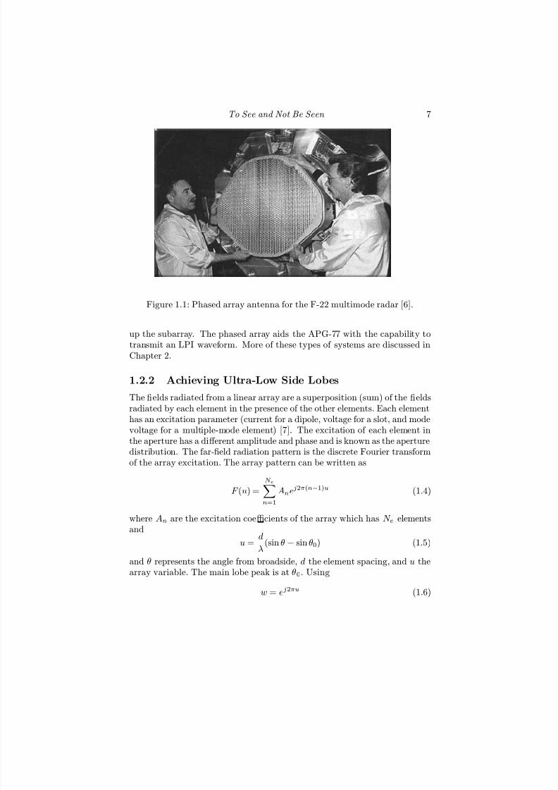
More advanced phased arrays are being developed where the transmit andreceive modules employ photonic switching (at optical frequencies), allowinghigh accuracy pointing and instantaneous beam positioning. They also al-low multiple pulse compression modulation signals to be scanned over largeangles. An example of a recent pioneering development is shown in Figure1.1. This figure shows the phased array used in the F-22 multimode fire
control radar [6]. The F-22’s AN/APG-77 electronically scanned array an-tenna is composed of several thousand transmit/receive modules, circulators,radiators, and manifolds assembled into subarrays and then integrated intoa complete array. The baseline design used thousands of hand-soldered flexcircuit interconnects to make the numerous radio frequency, digital, and di-rect current connections between the components and manifolds that make
7/17/2019 1596932341 Intercept Radar.pdf
http://slidepdf.com/reader/full/1596932341-intercept-radarpdf 38/891
To See and Not Be Seen 7
Figure 1.1: Phased array antenna for the F-22 multimode radar [6].
up the subarray. The phased array aids the APG-77 with the capability totransmit an LPI waveform. More of these types of systems are discussed inChapter 2.
1.2.2 Achieving Ultra-Low Side Lobes
The fields radiated from a linear array are a superposition (sum) of the fieldsradiated by each element in the presence of the other elements. Each elementhas an excitation parameter (current for a dipole, voltage for a slot, and modevoltage for a multiple-mode element) [7]. The excitation of each element inthe aperture has a diff erent amplitude and phase and is known as the aperturedistribution. The far-field radiation pattern is the discrete Fourier transformof the array excitation. The array pattern can be written as
F (u) =N en=1
Anej2π(n−1)u (1.4)
where An are the excitation coefficients of the array which has N e elementsand
u = d
λ(sin θ
−sin θ0) (1.5)
and θ represents the angle from broadside, d the element spacing, and u thearray variable. The main lobe peak is at θ0. Using
w = ej2πu (1.6)
7/17/2019 1596932341 Intercept Radar.pdf
http://slidepdf.com/reader/full/1596932341-intercept-radarpdf 39/891
8 Detecting and Classifying LPI Radar
(1.4) can be written as
F (u) =N en=1
Anwn−1 (1.7)
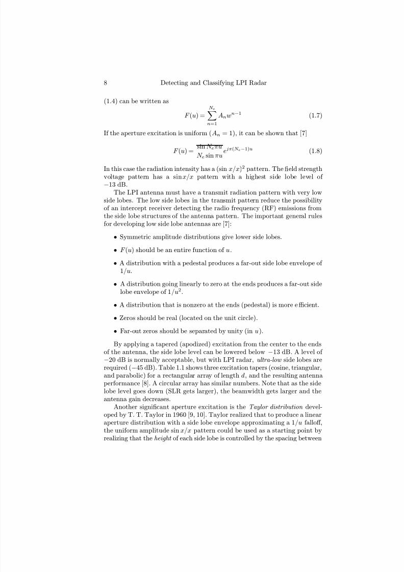
If the aperture excitation is uniform (An = 1), it can be shown that [7]
F (u) = sin N eπu
N e sin πuejπ(N e−1)u (1.8)
In this case the radiation intensity has a (sin x/x)2 pattern. The field strengthvoltage pattern has a sinx/x pattern with a highest side lobe level of −13 dB.
The LPI antenna must have a transmit radiation pattern with very low
side lobes. The low side lobes in the transmit pattern reduce the possibilityof an intercept receiver detecting the radio frequency (RF) emissions fromthe side lobe structures of the antenna pattern. The important general rulesfor developing low side lobe antennas are [7]:
• Symmetric amplitude distributions give lower side lobes.
• F (u) should be an entire function of u.
• A distribution with a pedestal produces a far-out side lobe envelope of 1/u.
• A distribution going linearly to zero at the ends produces a far-out sidelobe envelope of 1/u2.
• A distribution that is nonzero at the ends (pedestal) is more efficient.
• Zeros should be real (located on the unit circle).
• Far-out zeros should be separated by unity (in u).
By applying a tapered (apodized) excitation from the center to the endsof the antenna, the side lobe level can be lowered below −13 dB. A level of −20 dB is normally acceptable, but with LPI radar, ultra-low side lobes arerequired (−45 dB). Table 1.1 shows three excitation tapers (cosine, triangular,and parabolic) for a rectangular array of length d, and the resulting antennaperformance [8]. A circular array has similar numbers. Note that as the sidelobe level goes down (SLR gets larger), the beamwidth gets larger and the
antenna gain decreases.Another significant aperture excitation is the Taylor distribution devel-oped by T. T. Taylor in 1960 [9, 10]. Taylor realized that to produce a linearaperture distribution with a side lobe envelope approximating a 1/u falloff ,the uniform amplitude sin x/x pattern could be used as a starting point byrealizing that the height of each side lobe is controlled by the spacing between

7/17/2019 1596932341 Intercept Radar.pdf
http://slidepdf.com/reader/full/1596932341-intercept-radarpdf 40/891
To See and Not Be Seen 9
Table 1.1: Aperture Taper Functions and Resulting Characteristics3-dB Beamwidth Side Lobe Ratio Relative Full Null
Excitation (rad) (dB) Gain PositionCosineG(x) = cosN (πx/2); |x| < 1
N = 0 0.88λ/d 13.2 1.000 1.0λ/dN = 1 1.20λ/d 23.0 0.810 1.5λ/dN = 2 1.45λ/d 32.0 0.667 2.0λ/dN = 3 1.66λ/d 40.0 0.575 2.5λ/dN = 4 1.94λ/d 48.0 0.515 3.0λ/d
Triangular
G(x) = 1 − |x|; |x| ≤ 11.28λ/d 26.4 0.75 2.0λ/d
ParabolicG(x) = 1 − (1 −∆)x2; |x| < 1
∆ = 1.0 0.88λ/d 13.2 1.00 1.00λ/d∆ = 0.8 0.92λ/d 15.8 0.99 1.06λ/d∆ = 0.5 0.97λ/d 17.1 0.97 1.14λ/d∆ = 0 1.15λ/d 20.6 0.83 1.43λ/d
the aperture pattern factor zeros on each side of the side lobe. That is, sincethe sinc pattern has a 1/u side lobe envelope it is only necessary to modify theclose-in zeros to reduce the close-in side lobes. The shifting is accomplishedby setting zeros equal to
u =
n2 + B2 (1.9)
where B is a positive real parameter. The resulting pattern with the zerosshifted can be written as
F (u) = sinhπ
√ B2 − u2
π√
B2 − u2 (1.10)
for u ≤ B and
F (u) = sin π
√ B2 − u2
π√
B2 − u2 (1.11)
for u
≥B and is a modified sinc pattern where the one parameter B controls
all of the characteristics (side lobe level, beamwidth, directivity and so forth).Often known as the one-parameter Taylor scheme, the SLR (in decibels) canbe expressed as
SLR = 20 log sinhπB
πB + 13.2614 (1.12)

7/17/2019 1596932341 Intercept Radar.pdf
http://slidepdf.com/reader/full/1596932341-intercept-radarpdf 41/891
10 Detecting and Classifying LPI Radar
Table 1.2: Taylor Weighting Characteristics
Side Lobe Ratio (dB) B θ3 (rad)
13.26 0 0.8858λ/d15 0.3558 0.9230λ/d20 0.7386 1.0238λ/d25 1.0229 1.1160λ/d30 1.2762 1.2004λ/d35 1.5136 1.2782λ/d40 1.7415 1.3504λ/d45 1.9628 1.4182λ/d50 2.1793 1.4822λ/d
The SLR for the Taylor weighting as a function of the B parameter, and the3-dB beamwidth is shown in Table 1.2 as a function of the array length d andthe wavelength λ. Tables of circular aperture distributions and the designprocess for the Taylor scheme are given in [11].
1.2.3 Antenna Scan Patterns for Search Processing
LPI radar systems are often identified by the type of scanning the emitteruses. Scanning is the systematic movement of a radar’s antenna beam in aparticular pattern to search or track a target. The two methods of scanningan antenna beam are mechanically and electronically. The antenna can be
mechanically scanned by using gimbals to move the entire antenna aperture inany direction. Most often used are the two-dimensional arrays and parabolicreflectors (where instead of moving the reflector, the reflector feed can benutated to provide the scan coverage needed). The antenna can also be elec-tronically scanned by varying the phase between antenna elements (phasedarray).
The simplest case of a search radar scan is the use of a stationary pencilbeam that is fixed in elevation and rotated mechanically at a scan rate of ωr r s−1 to obtain an Ωa = 2π r coverage in azimuth and an Ωe = θe cov-erage in elevation. If range information is obtained for each beam positionin space, this is an example of a one-dimensional (1D) scan pattern. In thiscase the antenna searches or scans a solid angle field of view or scan volumeΩs = ΩaΩe = 2πθe sr (steradian). With a total solid angle coverage of the
sensor Ωs sr, the number of resolution elements is this value divided by theinstantaneous field of view of the antenna or
nr = Ωs
θaθe(1.13)
or 2π/θa. The elevation of the scan can also be changed after each complete

7/17/2019 1596932341 Intercept Radar.pdf
http://slidepdf.com/reader/full/1596932341-intercept-radarpdf 42/891
To See and Not Be Seen 11
Figure 1.2: LPI scan patterns: (a) conventional transmit-receive raster,(b) multibeam sector scan, and (c) omnitransmit multibeam receive.
rotation. This results in range, azimuth, and elevation information beingobtained from the field of view (e.g., a 2D scan pattern). To increase theefficiency of this 2D scan pattern, a set of n contiguous fixed pencil beamscan be stacked in elevation [12]. The azimuth scan can also be limited asshown in Figure 1.2(a) (azimuth dimension only) and, at the end of the limit,the elevation can be changed for the next azimuth scan (in the oppositedirection). This type of transmit-receive pattern is called a raster scan and isused frequently since it provides good coverage both in azimuth and elevation.An example of an LPI radar using this scan pattern is the Signaal’s SMART-L(mechanical scanning implementation) [13, 14]. The SMART-L is discussedfurther in Chapter 2.
The time T f s required to cover the solid angle of coverage Ωs is called
the frame time . For frame time T f , the dwell time (sometimes known astime-on-target) is
τ d = T f nr
s (1.14)
That is, for τ d s, energy is received from any point target at a range RT in

7/17/2019 1596932341 Intercept Radar.pdf
http://slidepdf.com/reader/full/1596932341-intercept-radarpdf 43/891
12 Detecting and Classifying LPI Radar
space that is illuminated by the transmitted radiation. The value of the dwelltime given by (1.14) is for one pencil beam scanning in azimuth and elevation.If the radar system uses a stacked beam configuration to scan in azimuth andelevation, the on target time will be increased by this factor
τ d = nT f
nr=
nT f θaθeΩs
s (1.15)
where n is the number of contiguous beams in the stack (usually six to 16[12]). Note that (1.15) does not include any scanning loss factor such as thetime necessary for the mechanically scanning antenna to move from the end-of-frame position to the beginning-of-frame position. Accounting for this lossLs > 1, the dwell time is expressed as
τ d = nT f θaθeΩsLs
s (1.16)
Phased arrays provide the ability to form multiple beams at diff erent frequen-cies to selectively search diff erent portions of the scan volume. In most cases,the transmit scan pattern of the LPI radar is controlled precisely to limit theillumination time to short and infrequent intervals (aperiodic scan cycle). Anexample of an LPI radar with this capability is described in the next section.
By subdividing the scan volume into N d sections, with every sector simul-taneously searched by a diff erent stack of beams using a diff erent frequency,the dwell time in each beam direction can also be increased by a factor of N d(see p. 530 in [15]) as
τ d = N dnT f θaθeΩsLs s (1.17)
Figure 1.2(b) shows the multibeam sector scan where the same scan volumeΩs is divided into N d sectors. For this technique (electronic scanning), eachsector has its own transmit-receive beam. Matching the coherent integrationtime to the dwell time, the power emitted in any one beam direction can bereduced by the factor 1/N d.
To electronically scan a phased array antenna a progressive phase shift istypically used [5]. To maintain a low side lobe level a method based on apattern search algorithm (PSA) has been recently proposed [16]. Instead of an amplitude taper (such as a Taylor excitation), low side lobe scanning canbe achieved using a phase taper . The PSA is a direct search algorithm. Bydefining a fitness function, the pattern search finds the best group of phase
variations to scan the main beam to the desired position while also reducingthe peak side lobe level [17].
Figure 1.2(c) shows a nonscanning single-beam transmit, multibeam re-ceive array where enough receive beams are formed to completely fill the scanvolume Ωs. This technique requires increased signal processing throughput

7/17/2019 1596932341 Intercept Radar.pdf
http://slidepdf.com/reader/full/1596932341-intercept-radarpdf 44/891
To See and Not Be Seen 13
and uses a single beamwidth nonscanning transmit antenna with many si-multaneous receive beams. Since no scanning is involved, the dwell time isequal to the frame time
τ d = T f s (1.18)
One important flexibility with this pattern is that the transmitter does notneed to be colocated with the receive array. An example of an LPI radar thatuses this technique is the omnidirectional LPI radar (OLPI) [18, 19]. TheOLPI is discussed further in Chapter 5.
As discussed in Part II (Chapter 11 through Chapter 18) of the text, inter-cept receivers use a variety of strategies to identify the LPI radar, includingangle of arrival, carrier frequency, scan rate, modulation period, bandwidth,and polarization. Randomly altering any of these parameters can therefore
provide confusion to the intercept receiver. Scan methodologies can be usedto help confuse identification if intercept occurs. For example, a scan tech-nique that attempts to confuse identification might include amplitude modu-lation of a monopulse array at conical scan frequencies that are not consideredthreatening. These types of scan methodologies require significant additionalprocessing requirements (and power) that limit the platforms that can carrythis type of capability.
1.2.4 Advanced Multifunction RF Concept
A radar that has the capability of forming multiple beams is the advanced multifunction RF concept (AMRFC). The AMRFC is a United States Navyprogram to investigate the capability to integrate radar (including an LPI
navigation radar in the high band 4.5—18.0 GHz), electronic warfare, andcommunication functions into a common set of wideband, low power levelRF apertures, where the functionality is mostly defined by the software [20].Consequently, the AMRFC reduces the number of topside RF system antennaapertures while increasing the eff ective functionality (through software), aswell as increasing the capability for ship signature control/reduction. TheAMRFC divides the frequency band into an optimal number of segments,based on cost and functionality, and then utilizes separate transmit and re-ceive apertures. The separate transmit and receive apertures allow full uti-lization of the entire time line for the transmitter as well as for the receiver.The transmit array is composed of dynamically allocable subarrays that aresectioned to form multiple simultaneous transmit beams . Since having morethan one signal present in a power amplifier is not currently feasible, each
transmit subarray is used by one function at a time. However, for the receivearray, more than one signal can be present simultaneously in a subarray.
The wideband arrays are electronically scanned and use solid state trans-mit and receive apertures. The use of the contiguous subarray architectureusing phase shifters at the element level and true time delays at the subar-

7/17/2019 1596932341 Intercept Radar.pdf
http://slidepdf.com/reader/full/1596932341-intercept-radarpdf 45/891
14 Detecting and Classifying LPI Radar
Figure 1.3: High band multifunction transmit array [22].
ray level results in high side lobes, due to subarray dispersion and gratinglobe generation [21]. The AMRFC phased arrays achieve side lobe reduc-tion by using an overlapping subarray architecture. Digital beamforming atthe subarray level makes it possible to generate multiple cluster beams andachieve pattern control or interference cancelation simultaneously. The over-lapping subarray allows the grating lobes to be pushed away from the mainlobe and shape the subarray patterns in such a way that all grating lobes aresuppressed in the subarray’s low side lobe region. The overlap architectureis further discussed in [21]. Figure 1.3 shows the high-band multifunction
transmit array that supports up to four simultaneous transmit beam con-figurations. Transmit array quadrants may also be combined to form largerapertures [22].
1.2.5 Transmitter Considerations
A conventional radar that uses a coherent pulse train has independent con-trol of both range and Doppler resolution. This type of radar waveformalso exhibits a range window that can be inherently free of side lobes. Themain drawback of a coherent pulse train waveform is the high peak-to-averagepower ratio put out by the transmitter. The average power is what deter-mines the detection characteristics of the radar. For high average power, ashort pulse (high range resolution) transmitter must have a high peak power,necessitating vacuum tubes and high voltages. The high peak power trans-missions can also easily be detected by noncooperative intercept receivers.The duty cycle dc for a pulsed emitter relates the average transmitted power
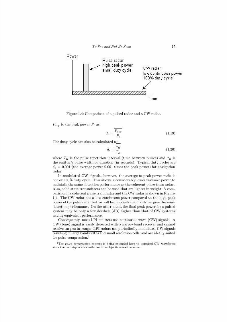
7/17/2019 1596932341 Intercept Radar.pdf
http://slidepdf.com/reader/full/1596932341-intercept-radarpdf 46/891
To See and Not Be Seen 15
Figure 1.4: Comparison of a pulsed radar and a CW radar.
P avg to the peak power P t as
dc = P avg
P t(1.19)
The duty cycle can also be calculated as
dc = τ R
T R(1.20)
where T R is the pulse repetition interval (time between pulses) and τ R isthe emitter’s pulse width or duration (in seconds). Typical duty cycles aredc = 0.001 (the average power 0.001 times the peak power) for navigationradar.
In modulated CW signals, however, the average-to-peak power ratio isone or 100% duty cycle. This allows a considerably lower transmit power tomaintain the same detection performance as the coherent pulse train radar.Also, solid state transmitters can be used that are lighter in weight. A com-parison of a coherent pulse train radar and the CW radar is shown in Figure1.4. The CW radar has a low continuous power compared to the high peakpower of the pulse radar but, as will be demonstrated, both can give the samedetection performance. On the other hand, the final peak power for a pulsedsystem may be only a few decibels (dB) higher than that of CW systemshaving equivalent performance.
Consequently, most LPI emitters use continuous wave (CW) signals. A
CW (tone) signal is easily detected with a narrowband receiver and cannotresolve targets in range. LPI radars use periodically modulated CW signalsresulting in large bandwidths and small resolution cells, and are ideally suitedfor pulse compression.1
1The pulse compression concept is being extended here to unpulsed CW waveformssince the techniques are similar and the objectives are the same.
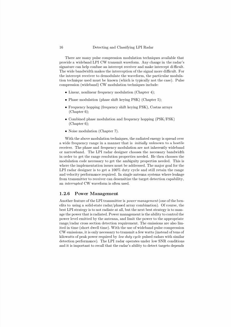
7/17/2019 1596932341 Intercept Radar.pdf
http://slidepdf.com/reader/full/1596932341-intercept-radarpdf 47/891
16 Detecting and Classifying LPI Radar
There are many pulse compression modulation techniques available thatprovide a wideband LPI CW transmit waveform. Any change in the radar’ssignature can help confuse an intercept receiver and make intercept difficult.The wide bandwidth makes the interception of the signal more difficult. Forthe intercept receiver to demodulate the waveform, the particular modula-tion technique used must be known (which is typically not the case). Pulsecompression (wideband) CW modulation techniques include:
• Linear, nonlinear frequency modulation (Chapter 4);
• Phase modulation (phase shift keying PSK) (Chapter 5);
• Frequency hopping (frequency shift keying FSK), Costas arrays(Chapter 6);
• Combined phase modulation and frequency hopping (PSK/FSK)(Chapter 6);
• Noise modulation (Chapter 7).
With the above modulation techniques, the radiated energy is spread overa wide frequency range in a manner that is initially unknown to a hostilereceiver. The phase and frequency modulation are not inherently widebandor narrowband. The LPI radar designer chooses the necessary bandwidthin order to get the range resolution properties needed. He then chooses themodulation code necessary to get the ambiguity properties needed. This iswhere the implementation issues must be addressed. The major goal for the
LPI radar designer is to get a 100% duty cycle and still retain the rangeand velocity performance required. In single antenna systems where leakagefrom transmitter to receiver can desensitize the target detection capability,an interrupted CW waveform is often used.
1.2.6 Power Management
Another feature of the LPI transmitter is power management (one of the ben-efits to using a solid-state radar/phased array combination). Of course, thebest LPI strategy is to not radiate at all, but the next best strategy is to man-age the power that is radiated. Power management is the ability to control thepower level emitted by the antenna, and limit the power to the appropriaterange/radar cross section detection requirement. The emissions are also lim-
ited in time (short dwell time). With the use of wideband pulse compressionCW emissions, it is only necessary to transmit a few watts (instead of tens of kilowatts of peak power required by low duty cycle pulsed radars with similardetection performance). The LPI radar operates under low SNR conditionsand it is important to recall that the radar’s ability to detect targets depends
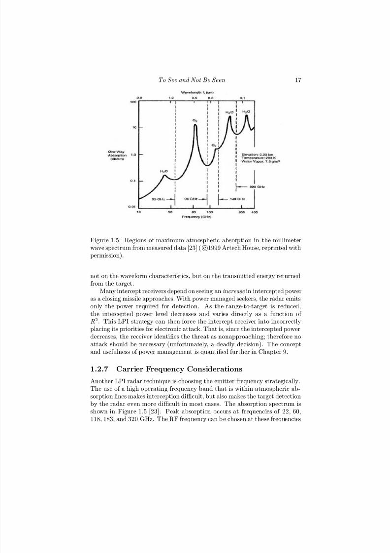
7/17/2019 1596932341 Intercept Radar.pdf
http://slidepdf.com/reader/full/1596932341-intercept-radarpdf 48/891
To See and Not Be Seen 17
Figure 1.5: Regions of maximum atmospheric absorption in the millimeterwave spectrum from measured data [23] ( c1999 Artech House, reprinted withpermission).
not on the waveform characteristics, but on the transmitted energy returnedfrom the target.
Many intercept receivers depend on seeing an increase in intercepted poweras a closing missile approaches. With power managed seekers, the radar emitsonly the power required for detection. As the range-to-target is reduced,the intercepted power level decreases and varies directly as a function of R2. This LPI strategy can then force the intercept receiver into incorrectlyplacing its priorities for electronic attack. That is, since the intercepted powerdecreases, the receiver identifies the threat as nonapproaching; therefore noattack should be necessary (unfortunately, a deadly decision). The conceptand usefulness of power management is quantified further in Chapter 9.
1.2.7 Carrier Frequency Considerations
Another LPI radar technique is choosing the emitter frequency strategically.
The use of a high operating frequency band that is within atmospheric ab-sorption lines makes interception difficult, but also makes the target detectionby the radar even more difficult in most cases. The absorption spectrum isshown in Figure 1.5 [23]. Peak absorption occurs at frequencies of 22, 60,118, 183, and 320 GHz. The RF frequency can be chosen at these frequencies

7/17/2019 1596932341 Intercept Radar.pdf
http://slidepdf.com/reader/full/1596932341-intercept-radarpdf 49/891
18 Detecting and Classifying LPI Radar
to maximize the attenuation in order to mask the transmit signal and limitreception by a hostile receiver (atmospheric attenuation shielding). Since thephysics of radar detection, however, depends only on the energy placed onthe target, LPI radars must still radiate sufficient eff ective radiated power(ERP) to accomplish detection. The loss for the radar due to atmosphericabsorption is over its total two-way path (out to the target and back), whilethe interceptor’s loss is over the one-way path (from the radar to the inter-cept receiver). Because of the high absorption of the emitter’s energy, thistechnique is always limited to short range systems. In the case of an inter-cept receiver on a radar target platform (such as a radar warning receiver),the advantage lies with the interceptor, since there is only one-half the pathloss. Another approach to achieving a lower probability of interception is tointerleave the LPI radar mode with an infrared sensor (dual mode approach),reducing the amount of time that the RF transmitter is radiating.
In summary, the important characteristics of LPI radar include widebandCW emission, low antenna side lobes with infrequent scan modulation, or theuse of a broad nonscanning transmitting beam combined with a stationary setof receive beams. Polarization modulation can also be used. The transmitteruses a wideband modulation technique (for the range resolution desired) incombination with power management and a strategic selection of frequencyto achieve the desired amount of atmospheric attenuation. That is, the wide-band signals are diff used in time, appearing in pseudorandom directions atpseudorandom times.
1.3 Pulse Compression—The Key to LPI Radar
The three general types of CW LPI radar architectures are the: (a) fre-quency modulating radar that includes FMCW and frequency shift keying(hopping), (b) the phase modulating radar that includes polyphase modula-tion (polyphase shift keying) and polytime modulation, and (c) the radar thatis a combination of both (a) and (b). The FMCW radar architecture is now inwidespread use. A block diagram of an FMCW radar is shown in Figure 1.6.The radar uses two antennas (one transmit and one receive). The transmittedwaveform for the FMCW radar is a linear (or nonlinear) frequency modulatedwaveform, and can be generated by using a direct digital synthesizer. Thereceived waveform is amplified by a low noise amplifier (LNA) and correlated(or mixed) with the transmit waveform in order to derive the target beat fre-quencies (homodyne detection). After the analog demodulation is used togenerate the intermediate frequency (IF) beat signals, they are digitized withan analog-to-digital converter. The digital signal with input signal-to-noiseratio SNRRi is processed by one or more fast Fourier transform signal proces-sors to derive the range (and possibly Doppler) profile. As shown in Figure1.6, a certain amount of integration is also commonly used to increase the

7/17/2019 1596932341 Intercept Radar.pdf
http://slidepdf.com/reader/full/1596932341-intercept-radarpdf 50/891
To See and Not Be Seen 19
Figure 1.6: Block diagram of an FMCW radar.
output signal-to-noise ratio SNRRo. Integration improves SNRRo since thenoise energy that accumulates in each range bin varies from one integrationperiod to the next, whereas the target return increases in direct proportion
to the integration time. Increasing the integration time can improve SNRRosignificantly. After integration, the target detection and tracking function isperformed.
The radar input SNRRi and output SNRRo are related by the processing gain of the signal processor as
P GR = SNRRoSNRRi
(1.21)
and depends on the time-bandwidth characteristics of the transmit signalmodulation as well as any noncoherent integration. The processing gain isalso referred to as the pulse compression ratio. A simple empirical formulacan also be used for the relationship between SNRRo and the probability of
detection P d, and the probability of false alarm P fa due to Albersheim isgiven as [12]SNRRo = A + 0.12AB + 1.7B (1.22)
where
A = ln
0.62
P fa
(1.23)

7/17/2019 1596932341 Intercept Radar.pdf
http://slidepdf.com/reader/full/1596932341-intercept-radarpdf 51/891
20 Detecting and Classifying LPI Radar
andB = ln
P d
1− P d
(1.24)
Here SNRRo is in linear units and not decibels.If the radar uses an FMCW waveform, the processing gain (excluding any
noncoherent integration) is the sweep or modulation period, tm, multipliedby the sweep (input) bandwidth, ∆F . That is,
P GR = tm∆F (1.25)
The modulation period tm in an FMCW radar plays the same role as T R ina pulsed radar and, in either case, both systems normally perform nonco-herent integration over as many such intervals as occupy the dwell time of
the beam. When noncoherent integration is performed for N I such intervals,the processing gain is increased by
√ N I . Also note that although Figure 1.6
shows an analog processing approach, the cross correlation (or homodyne de-tection) could also be done digitally. Additional details on FMCW LPI radardesign are discussed in Chapters 4, 7, 8, and 9.
A block diagram of a phase coded radar is shown in Figure 1.7. Thephase coded radar can also use a direct digital synthesizer to generate thetransmitted waveform. The phase coded radar transmit waveform is gener-ated using various phase modulations and/or frequency modulations. Thetarget return signal is amplified and downconverted using a local oscillator(LO), and digitized with an ADC. The digitized samples are then processedby a digital compressor, which cross correlates the transmitted code with thereceived signal. For phase modulation of a CW waveform using N c num-
ber of subcodes, the processing gain is the code period, T , multiplied by thetransmitted bandwidth, 1/tb, where tb is the subcode period. That is,
P GR = T (1/tb) = (N ctb)/tb = N c (1.26)
In the phase coded radar, the return signal is compressed using digital tech-niques, and noncoherent integration will also add to this processing gain.Additional details on phase shift keying radar are given in Chapter 5 and anexample of the processing gain distribution in a phase coded LPI radar isgiven in Section 5.12.
Note that in the FMCW radar example shown in Figure 1.6, the returnsignal from the target is compressed using an analog processor . AlthoughFigure 1.6 shows an analog processing approach, the processing could equally
well be digital. That is, the distinction between the two is the modulation , notthe method of processing or the location of the ADC in the receiver path. Forboth the frequency modulation and phase modulation LPI radar, the trans-mitted CW signal is coded with a reference signal to spread the transmittedenergy in frequency, to avoid detection and identification by the noncoop-erative intercept receiver. The reference signal can take the form of either
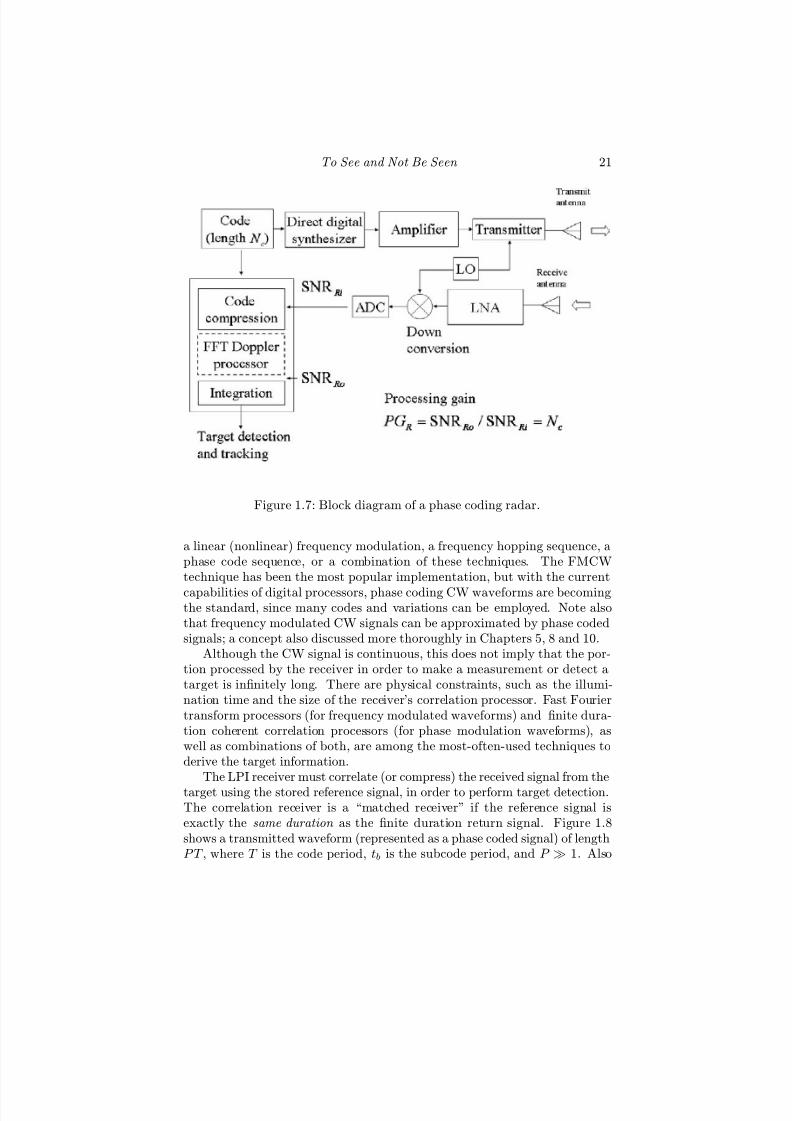
7/17/2019 1596932341 Intercept Radar.pdf
http://slidepdf.com/reader/full/1596932341-intercept-radarpdf 52/891
To See and Not Be Seen 21
Figure 1.7: Block diagram of a phase coding radar.
a linear (nonlinear) frequency modulation, a frequency hopping sequence, aphase code sequence, or a combination of these techniques. The FMCWtechnique has been the most popular implementation, but with the current
capabilities of digital processors, phase coding CW waveforms are becomingthe standard, since many codes and variations can be employed. Note alsothat frequency modulated CW signals can be approximated by phase codedsignals; a concept also discussed more thoroughly in Chapters 5, 8 and 10.
Although the CW signal is continuous, this does not imply that the por-tion processed by the receiver in order to make a measurement or detect atarget is infinitely long. There are physical constraints, such as the illumi-nation time and the size of the receiver’s correlation processor. Fast Fouriertransform processors (for frequency modulated waveforms) and finite dura-tion coherent correlation processors (for phase modulation waveforms), aswell as combinations of both, are among the most-often-used techniques toderive the target information.
The LPI receiver must correlate (or compress) the received signal from thetarget using the stored reference signal, in order to perform target detection.The correlation receiver is a “matched receiver” if the reference signal isexactly the same duration as the finite duration return signal. Figure 1.8shows a transmitted waveform (represented as a phase coded signal) of lengthP T , where T is the code period, tb is the subcode period, and P 1. Also

7/17/2019 1596932341 Intercept Radar.pdf
http://slidepdf.com/reader/full/1596932341-intercept-radarpdf 53/891
22 Detecting and Classifying LPI Radar
Figure 1.8: CW transmitted waveform and receiver reference signal [24, 25].
shown is the reference signal of length N T used in the receiver to compressthe received signal. Increasing the number of receiver reference waveformsN improves the target detection capabilities by increasing the resolution of the receiver response. The ambiguity analysis in Chapter 3 investigates thisconcept in more detail.
The LPI radar receiver can be modeled as a coherent correlation processorof finite duration N T as shown in Figure 1.9 [27]. The return signal is received
by the correlation receiver containing a reference signal which is the conjugateof N periods of the transmitted signal with N < P . The correlation receiverperforms a cross correlation between the received signal and a reference signal,whose envelope is the complex conjugate of N periods of the transmittedsignal envelope. To do this, the return signal (a binary phase coded signal inthis example) is first processed by a filter matched to a rectangular subcodeof length tb, followed by a detector that sends forward a one or a zero. Thedetected output signal is then piped through a tapped delay line where eachdelay D is tb s. The signal in the tapped delay line is first multiplied by thereference signal. The output of each multiplication is then summed separatelyfor each of the N code periods. The output of the sum block can then beweighted as C 1 through C N . With uniform weights, the first stage representsthe response of the receiver for a zero-Doppler shift signal (ν = 0), andis identical to the ideal autocorrelation function [26]. The response of thereceiver to a Doppler shifted signal ∆ν is obtained from the second stageby first multiplying the output (before addition) from the first stage with q 0
through q MN −1 where q = ej2π∆ν tb .In phase coded CW radar systems, return signals with Doppler do not cor-

7/17/2019 1596932341 Intercept Radar.pdf
http://slidepdf.com/reader/full/1596932341-intercept-radarpdf 54/891
To See and Not Be Seen 23
Figure 1.9: Doppler matrix correlation receiver matched to N periods of aphase coded signal of length M = 5 including weighting C i for Doppler sidelobe reduction [26] ( c1992 IEEE).

7/17/2019 1596932341 Intercept Radar.pdf
http://slidepdf.com/reader/full/1596932341-intercept-radarpdf 55/891
24 Detecting and Classifying LPI Radar
Figure 1.10: LPI radar and intercept receiver configuration.
relate perfectly because the Doppler shift changes the phase of the code acrossits period. This causes imperfect compression. Since the received signal isusually delayed and Doppler shifted, there is a special interest in the response
of a matched receiver, such as in Figure 1.9, to its own signal as a function of the two parameters delay and Doppler . To reduce the side lobes, weightingmay be factored into the reference signal. If the reference signal is weightedin order to reduce side lobes, the receiver is called a mismatched receiver . InChapter 3, the ambiguity response of these LPI receivers is discussed, as wellas the weighting functions.
1.4 Radar Detection Range
In this section, the maximum detection range for a CW radar is examined.The CW radar has a low continuous power with a 100% duty cycle. TheLPI radar and intercept receiver configuration is shown in Figure 1.10. To
determine the detection range of a CW radar, we start with the power densityat a range R m from an isotropic antenna given as [27]
P D = P CW 4πR2
W/m2 (1.27)
7/17/2019 1596932341 Intercept Radar.pdf
http://slidepdf.com/reader/full/1596932341-intercept-radarpdf 56/891
To See and Not Be Seen 25
where P CW is the average power of the CW transmitter in watts. Witha “directive” antenna having a transmit gain Gt along the boresight, thedirected power density at a range R from the radar is
P DD = P CW GtL1
4πR2 W/m2 (1.28)
The term L1(< 1) is the one-way atmospheric transmission factor
L1 = e−αRk (1.29)
where Rk is the range or path length in kilometers and α is the one-way extinc-tion coefficient or power attenuation coefficient in nepers per km (Np/km).The one-way attenuation coefficient as a function of frequency is shown inFigure 1.5 in more useful engineering units (dB/km). To convert dB/km intoNp/km, multiply the attenuation coefficient in Figure 1.5 by 0.23.
The reradiated power density reflected off a target with radar cross sectionσT (m2) at range RT and appearing back at the radar is
P DDR = P CW GtL2
4πR2T
σT
4πR2T
W/m2 (1.30)
where RT is the range between the LPI radar and the target. The termL2(< 1) is the two-way atmospheric transmission factor
L2 = e−2αRk (1.31)
The LPI radar captures the reflected energy with its receive antenna. Thereceived signal power at the radar receiver from the target is
P RT = P CW GtL2
4πR2T LRT LRR
σT
4πR2T
Ae (1.32)
where Ae is the eff ective area of the radar receive antenna and related to thereceive antenna gain Gr as
Ae = Grλ
2
4π (1.33)
and LRT is the loss between the radar’s transmitter and antenna, and LRRis the loss between the radar’s antenna and receiver. Substituting (1.33) into(1.32) gives the reflected power at the radar receiver as
P RT = P CW GtGrλ2L2σT
(4π)3R4T LRT LRR
(1.34)
It is often necessary to know the minimum input signal power at which areceiver can detect and process an incoming target signal. This is called the
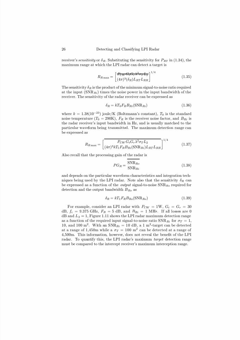
7/17/2019 1596932341 Intercept Radar.pdf
http://slidepdf.com/reader/full/1596932341-intercept-radarpdf 57/891
26 Detecting and Classifying LPI Radar
receiver’s sensitivity or δ R. Substituting the sensitivity for P RT in (1.34), themaximum range at which the LPI radar can detect a target is
RRmax =
P CW GtGrλ
2σT L2
(4π)3(δ R)LRT LRR
1/4(1.35)
The sensitivity δ R is the product of the minimum signal-to-noise ratio requiredat the input (SNRRi) times the noise power in the input bandwidth of thereceiver. The sensitivity of the radar receiver can be expressed as
δ R = kT 0F RBRi(SNRRi) (1.36)
where k = 1.38(10−23) joule/K (Boltzmann’s constant), T 0 is the standard
noise temperature (T 0 = 290K), F R is the receiver noise factor, and BRi isthe radar receiver’s input bandwidth in Hz, and is usually matched to theparticular waveform being transmitted. The maximum detection range canbe expressed as
RRmax =
P CW GtGrλ
2σT L2
(4π)3kT 0F RBRi(SNRRi)LRT LRR
1/4(1.37)
Also recall that the processing gain of the radar is
P GR = SNRRoSNRRi
(1.38)
and depends on the particular waveform characteristics and integration tech-
niques being used by the LPI radar. Note also that the sensitivity δ R canbe expressed as a function of the output signal-to-noise SNRRo required fordetection and the output bandwidth BRo as
δ R = kT 0F RBRo(SNRRo) (1.39)
For example, consider an LPI radar with P CW = 1W, Gt = Gr = 30dB, f c = 9.375 GHz, F R = 5 dB, and BRi = 1 MHz. If all losses are 0dB and L2 = 1, Figure 1.11 shows the LPI radar maximum detection rangeas a function of the required input signal-to-noise ratio SNRRi for σT = 1,10, and 100 m2. With an SNRRi = 10 dB, a 1 m2-target can be detectedat a range of 1,450m while a σT = 100 m2 can be detected at a range of 4,500m. This information, however, does not reveal the benefit of the LPI
radar. To quantify this, the LPI radar’s maximum target detection rangemust be compared to the intercept receiver’s maximum interception range.

7/17/2019 1596932341 Intercept Radar.pdf
http://slidepdf.com/reader/full/1596932341-intercept-radarpdf 58/891
To See and Not Be Seen 27
Figure 1.11: LPI radar maximum detection range for σT =1, 10, 100 m2.
1.5 Interception Range
From the configuration shown in Figure 1.10, the signal power available atthe intercept receiver from the LPI radar is
P IR = P CW G
tL1
4πR2I LRT LIR
GI λ
2
4π
(1.40)
where RI is the range from the LPI radar to the intercept receiver, and G
t isthe gain of the LPI radar’s transmit antenna in the direction of the interceptreceiver. Also, GI is the gain of the intercept receiver’s antenna, and LIRrepresents the losses from the antenna to the receiver. If the intercept receiverdetects the radar main lobe, G
t = Gt. If the intercept receiver detects theradar emission from the side lobes, G
t represents the gain of the antenna sidelobe in the intercept receiver direction. Replacing the signal power available,P IR , by the intercept receiver’s sensitivity, δ I , the maximum interceptionrange of the receiver can be defined as
RI max =
P CW G
tGI L1λ2
(4π)2LRT LIR(δ I ) (1.41)
where the sensitivity in the intercept receiver is similarly defined as
δ I = kT 0F I BI (SNRIi) (1.42)

7/17/2019 1596932341 Intercept Radar.pdf
http://slidepdf.com/reader/full/1596932341-intercept-radarpdf 59/891
28 Detecting and Classifying LPI Radar
Figure 1.12: Block diagram of an intercept receiver model showing both thepredetection stage and the postdetection stage.
where F I is the intercept receiver noise factor, BI is the bandwidth of theintercept receiver, and SNRIi is the SNR at the intercept receiver signalprocessor input. The maximum interception range can then be expressed as
RI max =
P CW G
tGI L1λ2
(4π)2LRT LIRkT 0F I BI (SNRIi) (1.43)
Also recall that the intercept receiver processing gain P GI is defined as
P GI = SNRIoSNRIi
(1.44)
Contrary to communication or radar system receiver design where the band-width is matched to the known transmitted signal, the intercept receiver doesnot know the exact nature of the threat signals. Figure 1.12 shows a blockdiagram of an intercept receiver model showing the predetection stage andthe postdetection stage. The three major components include the RF (prede-tection) amplifier with bandwidth BIR , the detector (e.g., square law), andthe postdetection video amplifier with bandwidth BIV .
In the intercept receiver design it is most often necessary to match thefront-end RF bandwidth BIR to the largest coherent radar bandwidth ex-pected, and to match the video bandwidth BIV to the inverse of the smallestradar coherent integration time expected tI . Exact analysis of intercept re-ceiver bandwidths and sensitivities is complicated. However, since the δ I in(1.42) is dependent on the intercept receiver’s overall bandwidth, it is desir-
able to have an approximate expression for BI that includes the eff ects of both the predetection and postdetection bandwidths. The approximate ex-pressions have been derived by Klipper [28]. The bandwidth of the interceptreceiver for BIR >> BIV (which is typically the case) can be expressed as
BI =
2BIRBIV (1.45)

7/17/2019 1596932341 Intercept Radar.pdf
http://slidepdf.com/reader/full/1596932341-intercept-radarpdf 60/891
To See and Not Be Seen 29
for a square law detector and
BI = 1
2
2BIRBIV (1.46)
for a linear detector. The time-bandwidth product or processing gain of theintercept receiver often takes the form of [3]
P GI = (tI BIR)γ (1.47)
and depends on the efficiency γ . The noncoherent integration efficiency ison the order of 0.5 ≤ γ ≤ 0.8 [3]. For example, if an FMCW radar has amodulation bandwidth of ∆F = 55 MHz, and a coherent integration timeof tm = 1 ms, the processing gain of the radar is P GR = tm∆F = 55,000,
whereas the processing gain of the intercept receiver is only P GI = √ tm∆F =234 (γ = 0.5). This is the real origin of the LPI radar .
Figure 1.13 shows the maximum interception range of the intercept re-ceiver as a function of the required input SNRIi . This is the maximum rangeat which the passive intercept receiver can intercept an LPI radar operatingat f c = 9.375 GHz with a transmitting antenna gain Gt = 1,000 and trans-mitter power P CW = 1W. The intercept receiver has an isotropic antennawith gain GI = 1, a noise figure F I = 5 dB, and LRT , LIR = 1. Both asquare law and linear detector configuration are considered with BIV = 1kHz (radar coherent integration time tm = 1 ms). The performance for pre-detection bandwidths of BIR = 60 MHz and 120 MHz is also compared. Notethat the smaller the required predetection RF bandwidth is, the larger themaximum interception range. The use of a square law detector over a lineardetector also gives a larger interception range.
1.6 Comparing Radar Range and Interception
Range
The radar sensitivity δ R (1.36) and intercept receiver sensitivity δ I (1.42) canbe used to quantify the benefit of the LPI radar. The ratio of the interceptreceiver sensitivity to the radar sensitivity is
δ = δ I
δ R=
kT 0BI F I kT 0BRiF R
SNRIiSNRRi
(1.48)
In terms of the processing gains and output signal-to-noise ratios, the ratioof sensitivities can be expressed as
δ = F I BI F RBRo
SNRIoSNRRo
P GRP GI
(1.49)
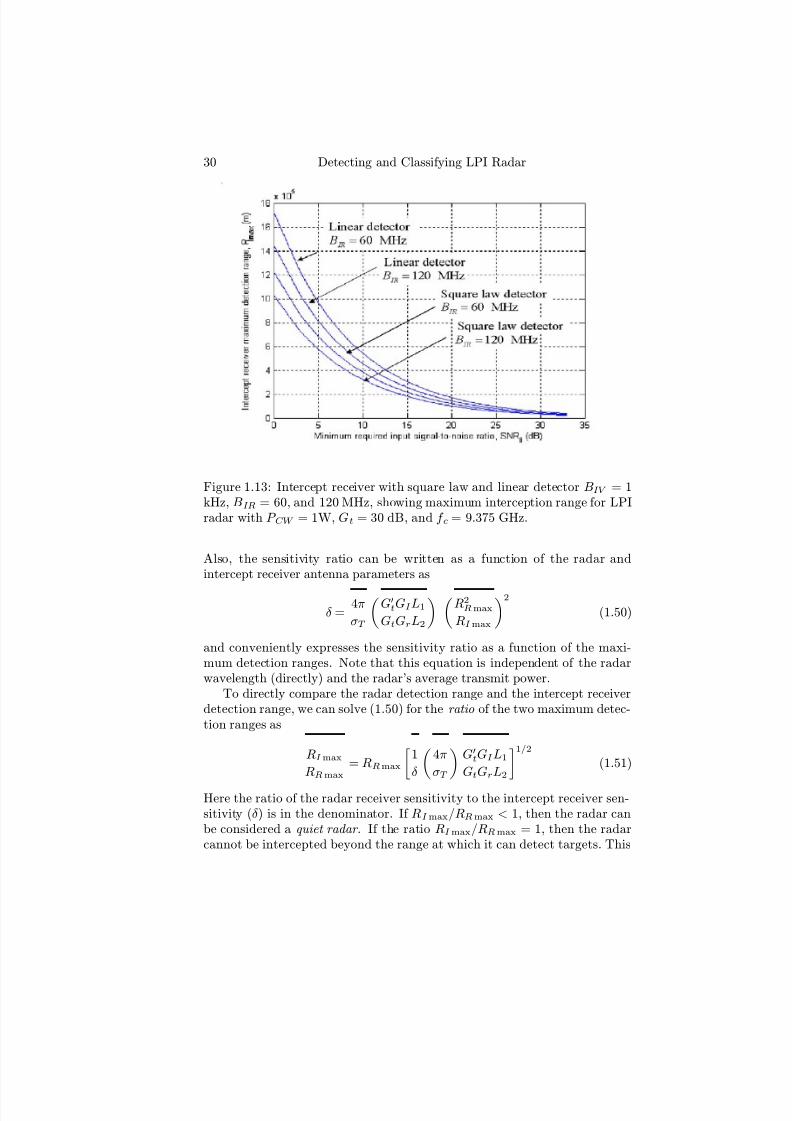
7/17/2019 1596932341 Intercept Radar.pdf
http://slidepdf.com/reader/full/1596932341-intercept-radarpdf 61/891
30 Detecting and Classifying LPI Radar
Figure 1.13: Intercept receiver with square law and linear detector BIV = 1kHz, BIR = 60, and 120 MHz, showing maximum interception range for LPIradar with P CW = 1W, Gt = 30 dB, and f c = 9.375 GHz.
Also, the sensitivity ratio can be written as a function of the radar andintercept receiver antenna parameters as
δ = 4π
σT
G
tGI L1
GtGrL2
R2Rmax
RI max
2
(1.50)
and conveniently expresses the sensitivity ratio as a function of the maxi-mum detection ranges. Note that this equation is independent of the radarwavelength (directly) and the radar’s average transmit power.
To directly compare the radar detection range and the intercept receiverdetection range, we can solve (1.50) for the ratio of the two maximum detec-tion ranges as
RI max
RRmax= RRmax
1
δ 4π
σT G
tGI L1
GtGrL2 1/2
(1.51)
Here the ratio of the radar receiver sensitivity to the intercept receiver sen-sitivity (δ ) is in the denominator. If RI max/RRmax < 1, then the radar canbe considered a quiet radar . If the ratio RI max/RRmax = 1, then the radarcannot be intercepted beyond the range at which it can detect targets. This

7/17/2019 1596932341 Intercept Radar.pdf
http://slidepdf.com/reader/full/1596932341-intercept-radarpdf 62/891
To See and Not Be Seen 31
is an important consequence. With RI max/RRmax = 1, from (1.51)
RRmax =
δ σT
4π
L2GtGrL1G
tGI
1/2(1.52)
Note that this is the maximum detection range of the LPI radar without being intercepted by the intercept receiver. This is also the noncooperativereceiver’s maximum intercept range. An example is developed next in orderto examine this result.
To illustrate (1.52), the detection of an LPI radar is considered with bothmain lobe detection (G
t = Gt = 1,000) and side lobe detection with sidelobes G
t = 0.1 (40 dB below main beam). The target RCS σT = 1m2 andwe consider that L2 = L1 = 1. The intercept receiver antenna gain GI = 1.
Figure 1.14 shows the sensitivity ratio as a function of the maximum detectionrange for both main lobe intercepts and side lobe intercepts. The figure showsthe large diff erence in the sensitivity ratio due to the diff erence of detectingthe radar in the side lobes versus the main lobes. The figure shows that asensitivity ratio of 60 dB is required for a maximum radar detection range,noncooperative intercept range of ≈ 104m (intercept receiver intercepting themain lobe). If the intercept receiver is required to intercept the radar in the side lobes at this range, the intercept receiver must decrease the sensitivityratio from 60 dB to 20 dB. From (1.49), one of the ways this can happenis when the intercept receiver increases its processing gain P GI which istypically difficult to do without sophisticated signal processing techniques(discussed in Part II).
1.7 The Pilot LPI Radar
During 1988, the Philips Research Laboratory developed a “quiet” radarknown as Pilot, which was marketed by the then Philips’ subsidiaries PEABin Sweden and Signaal in the Netherlands. With the sell-off of Philips’ de-fense assets, PEAB was taken over by Bofors (subsequently CelsiusTech andnow SaabTech), and maintained the name of Pilot for this radar. For itspart, Signaal was taken over by the then Thomson-CSF (now Thales), andmodified and improved the FMCW Pilot concept and changed the name of the radar to Scout.
The Pilot is a well-published example of an FMCW tactical navigationLPI radar [29—33]. It can easily be added on to an existing navigation radar,
retaining the original X-band antenna, transceiver, and display system. Ina tactical situation, the Pilot can be switched out and the pulsed radar canbe switched in when higher signal-to-noise ratios are required. It also hasstandard video output to simplify integration with standard pulsed navigationradar.

7/17/2019 1596932341 Intercept Radar.pdf
http://slidepdf.com/reader/full/1596932341-intercept-radarpdf 63/891
32 Detecting and Classifying LPI Radar
Figure 1.14: LPI radar maximum detection range as a function of thesensitivity ratio δ .
The Pilot uses an FMCW 1-kHz sweep repetition frequency with a lownoise figure (F R = 5 dB) and very low output power to ensure that it is un-
detectable by hostile intercept receivers. Other features include a 1,024-pointFFT (512 range cells) high range resolution (2.7m to 86m), high reliability,small lightweight designs, and ease of installation. The technical parame-ters are given in Table 1.3. Note that 1 nautical mile (nmi) = 1.852 km.Figure 1.15 shows the equipment that makes up the Pilot Mk3 version thatwas developed by Saab Bofors Dynamics AB (formerly CelsiusTech Electron-ics). The MK3 has an improved LPI performance by combining an FMCWwaveform with frequency agility . In this section we use the formulations inprevious sections to quantify the Pilot performance.
The most important LPI characteristics of the Pilot are that it uses onlyone low side lobe antenna, transmits a maximum CW power of only 1W, anduses an FMCW waveform with a variable modulation bandwidth ∆F to varythe range resolution. We will return to a detailed discussion of this type of
LPI radar modulation in Chapter 4. Below, several examples are shown toillustrate the performance of the radar and compare it with a conventionallow pulse repetition frequency (LPRF) navigation radar.
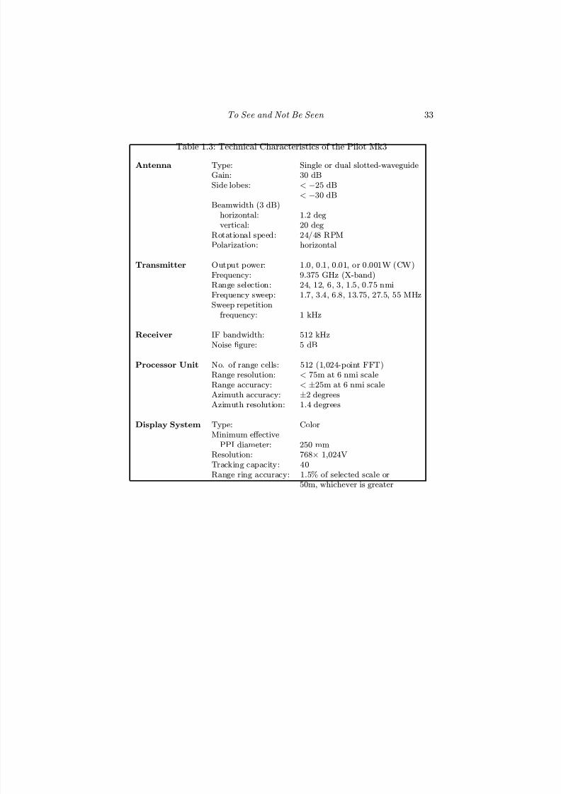
7/17/2019 1596932341 Intercept Radar.pdf
http://slidepdf.com/reader/full/1596932341-intercept-radarpdf 64/891
To See and Not Be Seen 33
Table 1.3: Technical Characteristics of the Pilot Mk3
Antenna Type: Single or dual slotted-waveguideGain: 30 dBSide lobes: < −25 dB
< −30 dBBeamwidth (3 dB)
horizontal: 1.2 degvertical: 20 deg
Rotational speed: 24/48 RPMPolarization: horizontal
Transmitter Output power: 1.0, 0.1, 0.01, or 0.001W (CW)
Frequency: 9.375 GHz (X-band)Range selection: 24, 12, 6, 3, 1.5, 0.75 nmiFrequency sweep: 1.7, 3.4, 6.8, 13.75, 27.5, 55 MHzSweep repetition
frequency: 1 kHz
Receiver IF bandwidth: 512 kHzNoise figure: 5 dB
Processor Unit No. of range cells: 512 (1,024-point FFT)Range resolution: < 75m at 6 nmi scaleRange accuracy: < ±25m at 6 nmi scaleAzimuth accuracy: ±2 degreesAzimuth resolution: 1.4 degrees
Display System Type: ColorMinimum eff ective
PPI diameter: 250 mmResolution: 768× 1,024VTracking capacity: 40Range ring accuracy: 1.5% of selected scale or
50m, whichever is greater

7/17/2019 1596932341 Intercept Radar.pdf
http://slidepdf.com/reader/full/1596932341-intercept-radarpdf 65/891
34 Detecting and Classifying LPI Radar
Figure 1.15: Equipment that makes up the Pilot Mk3.
Example 1: Sensitivity
It is known that the Pilot radar using only P CW = 1W has a maximumdetection range of RRmax = 28 km for a σT = 100m2 target. Using thesystem parameter values given in Table 1.3, determine the sensitivity δ R of the Pilot receiver. Using (1.35),
δ R = P CW GtGrλ
2σT L2
(4π)3(R4Rmax)LRT LRR
(1.53)
with Gt = Gr = 1,000, λ = 0.032m, and substitution of the Pilot parameters(assuming that L2 = LRT = LRR = 1)
δ R = 1 ∗ (1,000)2 ∗ (0.032)2 ∗ 100
(4π)3 ∗ (28,000)4 = 8.4 × 10⁻¹⁷ W (1.54)
or −130 dBm.

7/17/2019 1596932341 Intercept Radar.pdf
http://slidepdf.com/reader/full/1596932341-intercept-radarpdf 66/891
To See and Not Be Seen 35
Example 2: Required Input SNR
Figure 1.6 shows SNRRi is located at the output of the ADC (input to thesignal processor). Since the Pilot radar uses down conversion processing totranslate the received signal frequency to IF, BRi = 512 kHz which corre-sponds to the Pilot’s IF bandwidth in Table 1.3. To determine the inputsignal-to-noise ratio SNRRi we know from (1.36)
δ R = kT 0F RBRi(SNRRi) (1.55)
Using F R = 100.5, k T 0 = 4 × 10⁻²¹, and BRi = 512 kHz,
SNRRi = δ R
kT 0F RBRi= 0.013 (1.56)
or −19 dB.
Example 3: Processing Gain, Output SNR
For the maximum modulation bandwidth ∆F = 55 MHz, we can calculatethe processing gain P GR and the output SNRRo. The processing gain for a single sweep can be calculated from (1.25) as
P GR = tm∆F = 55,000 (1.57)
The corresponding output SNR is then
SNRRo = P GR(SNRRi) = 715 (1.58)
or 28 dB. The addition of noncoherent integration of more than one modula-tion period within the signal processor can increase the processing gain andthe SNRRo.
Example 4: Comparison with Conventional Pulsed Radar
If the emitter is a conventional low pulse repetition frequency (PRF) naviga-tion radar with a peak power of P t = 10 kW, pulse width of τ = 1 μs, andF R = 5 dB, neglecting losses, (a) determine the maximum detection range fora σT = 100m2 target if the minimum required receiver input signal-to-noise
ratio SNRRi = −1.7 dB and (b) for the intercept system above (δ I = −80dBmi), determine the maximum intercept range (main lobe intercepts). For(a), we can use (1.37) with P CW replaced by the peak power P t = 10 kW and

7/17/2019 1596932341 Intercept Radar.pdf
http://slidepdf.com/reader/full/1596932341-intercept-radarpdf 67/891
36 Detecting and Classifying LPI Radar
Table 1.4: Pilot Detection and Intercept Range CalculationsRadar Detection Intercept Range
Range (km) (km)Radar Intercept Intercept InterceptOutput 100 m2 1 m2
δ I δ I δ I
Power target target −40 dBmi −60 dBmi −80 dBmi
Pilot Mk21 W 28 8.8 0.25 2.5 2.50.1 W 16 5.0 0 0.8 8.010 mW 9.0 2.8 0 0.25 2.51 mW 5.0 1.5 0 0 0.8LPRF Radar10 kW 49.6 15.7 25 254 2.546
BRi = 1(106) = 1/τ .2
Rconv =
P tGtGrλ
2σT L2
(4π)3kT 0F RBRi(SNRRi)
1/4(1.59)
or
Rconv =
104 ∗ (1, 000)2 ∗ (0.032)2 ∗ 100
(4π)3 ∗ 4(10−21) ∗ 100.5 ∗ 1(106) ∗ 0.67
1/4(1.60)
or Rconv = 49.6 km. For (b), the maximum intercept range can be determinedfrom (1.41) as
RI max = P tGtGI L1λ
2
(4π)2δ I LRT LIR1/2
(1.61)
or
RI max =
10, 000 ∗ 1(103) ∗ (1) ∗ (0.032)2
(4π)2 ∗ 10−11.0
1/2(1.62)
or RI max = 2,546 km. A summary of the above results and other additionalcalculations are shown in Table 1.4. Note that we use dBmi to represent dBin mW with reference to a system containing an isotropic antenna GI = 1.
1.8 Concluding Remarks
LPI modulation techniques include frequency modulation such as FMCW andfrequency shift keying. Also used are phase modulations such as the polyphase
2A pulsed radar receiver usually has an input bandwidth that is matched to the transmit-ted pulse width τ at either the null-to-null bandwidth (BRi = 2/τ ) or the 3-dB bandwidth(BRi = 1/τ ).
7/17/2019 1596932341 Intercept Radar.pdf
http://slidepdf.com/reader/full/1596932341-intercept-radarpdf 68/891
To See and Not Be Seen 37
codes Frank, P1, P2, P3, P4, and polytime codes T1, T2, T3, and T4. Thereare several trade-off s in the design of LPI emitters. The LPI modulations arenot inherently wideband (or narrowband). The radar designer chooses theemitter bandwidth to achieve the range resolution properties needed. He alsochooses the particular code to get the ambiguity (delay Doppler frequency)code properties needed. Implementation issues must also be addressed (suchas digital versus analog). The major question is how to get a 100% duty factorand still get the desired range and velocity performance needed to performthe mission.
A larger processing gain can be obtained by wideband coding of the trans-mitted waveform with a modulation that is known only to itself. What isimportant is if the coding degrades the sensitivity of the intercept receiverrelative to the radar receiver. The coding may or may not have an eff ect onthe sensitivity ratio δ . For example, if the intercept receiver is a simple crys-tal video receiver, then the wideband coding has no eff ect on the interceptreceiver’s sensitivity. That is, the value of coding in LPI has to do with theeff ect imposed on the interceptor—not on the radar if it uses a matched filter.
The intercept receiver bandwidth BI is typically larger than the radar’scoherent bandwidth in order to maximize the detection of the unknown signalsand perform well against large time-bandwidth signals. Also, the interceptreceiver’s noncoherent integration time should match the radar’s coherentintegration time. The design of the modern intercept receiver, however, is acomplicated issue due to the combined capability of an electronic support (ES)receiver, radar warning receiver (RWR), and electronic intelligence (ELINT)receiver in a single system, and many architectures are possible. These issues
are addressed in further detail in Part II.
References
[1] Wiley, R. G., Electronic Intelligence: The Interception of Radar Signals ,Artech House, Dedham, MA, 1985.
[2] Schleher, D. C., “Low probability of intercept radar,” Record of the IEEE
International Radar Conference , pp. 346—349, 1985.
[3] Schrick, G., and Wiley, R. G., “Interception of LPI radar signals,” Record of
the IEEE International Radar Conference , Arlington, VA, pp. 108—111, May7—10, 1990.
[4] Ruff e, L. I., and Stott, G. F., “LPI considerations for surveillance radars,”Proc. of the International Conference on Radar , Brighton, U.K., pp. 200—
202, 1992.[5] Balanis, C. A., Antenna Theory Analysis and Design , Harper and Row, Pub-
lishers, New York, 1982.
[6] http://www.f22fighter.com/radar.htm andhttp://www.globalsecurity.org/military/systems/aircraft/f-22-avionics.htm(APG-77).

7/17/2019 1596932341 Intercept Radar.pdf
http://slidepdf.com/reader/full/1596932341-intercept-radarpdf 69/891
38 Detecting and Classifying LPI Radar
[7] Rudge, A. W., Milne, K., Olver, A. D., and Knight, P., The Handbook of Antenna Design, Vol. 2 , IET, 1983.
[8] Forrest, J. R., “Antenna design tradeoff s examined,” Microwave Systems
News , Vol. 13, No. 12, pp. 237-243, Nov. 1983.
[9] Taylor, T. T., “Design of circular apertures for narrow beamwidth and lowsidelobes,” IRE Trans. on Antennas and Propagation, AP-8, pp. 17—22,1960.
[10] Hansen, R. C., “Tables of Taylor distributions for circular aperture antennas,”IRE Trans. on Antennas and Progagation, pp. 23—26, Jan. 1960.
[11] Hansen, R. C., “A one parameter circular aperture distribution with narrowbeamwidth and low sidelobes,” IEEE Trans. on Antennas and Propagation,
pp. 477—480, July, 1976.
[12] Skolnik, M. I., Introduction to Radar Systems, 3rd Edition , McGraw-Hill,Boston, MA, 2001.
[13] http://www.naval-technology.com/contractors/weapon control/thales5/(SMART-L).
[14] Pietrasinski, J. F., Brenner, T. W., and Lesnik, C. J., “Selected tendenciesof modern radars and radar systems development,” 12th International Con-
ference on Microwaves and Radar , MIKON ’98 , Krakow, Poland, Vol. 1, pp.133—137, May 20-22, 1998.
[15] Stimson, G. W., Introduction to Airborne Radar, 2nd Edition , Scitech Pub-lishing Inc., Mendham, NJ, 1998.
[16] Ebadi, S., Forouraghi, K., and Sattarzadef, S. A., “Optimum low sidelobelevel phased array antenna design using pattern search algorithms,” IEEE
International Symposium on Antennas and Propagation , pp. 770—773, Vol.
1B, Washington DC, 2005.[17] Ebadi, S., Forouraghi, K., “Pattern scanning in low sidelobe phased array
antennas using pattern search algorithms,” Proceedings of the 4th European
Radar Conference , pp. 347—349, 2007.
[18] Wirth, W. D., “Long term coherent integration for a floodlight radar,” Record
of the IEEE International Radar Conference , pp. 698—703, 1995.
[19] Wirth, W. D., Radar Techniques Using Array Antennas, IEE Radar, Sonar,Navigation, and Avionics Series 10, 2001.
[20] Hughes, P. K., and Choe, J. Y., “Overview of advanced multifunction RFsystem (AMRFS),” Proc. of the IEEE International Conference on Phased
Array Systems and Technology, pp. 21—24, 2000.
[21] Ching-Tai Lin, and Ly, Hung, “Sidelobe reduction through subarray overlap-ping for wideband arrays,” Proc. of IEEE Radar Conference , pp. 228—233
2001.[22] Tavik, G. C., Hilterbrick, C. L., Evins, J. B., Alter, J. J., Crnkovich, J. G.,
de Graaf, J. W., Habicht, W., Hrin, G. P., Lessin, S. A., Wu, D. C., andHagewood, S. M., “The advanced multifunction RF concept,” IEEE Trans.
on Microwave Theory and Techniques, Vol. 53, No. 3, pp. 1009—1020, March2005.
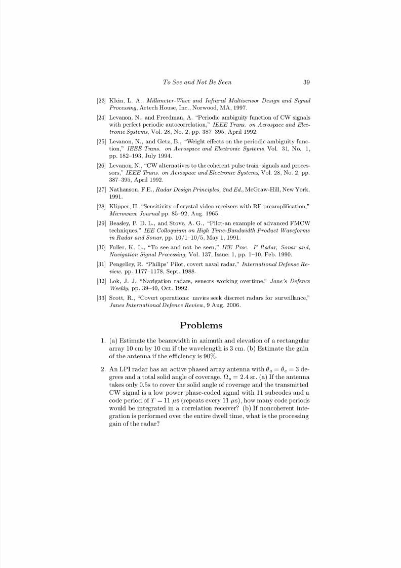
7/17/2019 1596932341 Intercept Radar.pdf
http://slidepdf.com/reader/full/1596932341-intercept-radarpdf 70/891
To See and Not Be Seen 39
[23] Klein, L. A., Millimeter-Wave and Infrared Multisensor Design and Signal Processing , Artech House, Inc., Norwood, MA, 1997.
[24] Levanon, N., and Freedman, A. “Periodic ambiguity function of CW signalswith perfect periodic autocorrelation,” IEEE Trans. on Aerospace and Elec-
tronic Systems , Vol. 28, No. 2, pp. 387—395, April 1992.
[25] Levanon, N., and Getz, B., “Weight eff ects on the periodic ambiguity func-tion,” IEEE Trans. on Aerospace and Electronic Systems , Vol. 31, No. 1,pp. 182—193, July 1994.
[26] Levanon, N., “CW alternatives to the coherent pulse train—signals and proces-sors,” IEEE Trans. on Aerospace and Electronic Systems , Vol. 28, No. 2, pp.387—395, April 1992.
[27] Nathanson, F.E., Radar Design Principles, 2nd Ed., McGraw-Hill, New York,
1991.[28] Klipper, H. “Sensitivity of crystal video receivers with RF preamplification,”
Microwave Journal pp. 85—92, Aug. 1965.
[29] Beasley, P. D. L., and Stove, A. G., “Pilot-an example of advanced FMCWtechniques,” IEE Colloquium on High Time-Bandwidth Product Waveforms
in Radar and Sonar , pp. 10/1—10/5, May 1, 1991.
[30] Fuller, K. L., “To see and not be seen,” IEE Proc. F Radar, Sonar and,
Navigation Signal Processing, Vol. 137, Issue: 1, pp. 1—10, Feb. 1990.
[31] Pengelley, R. “Philips’ Pilot, covert naval radar,” International Defense Re-
view, pp. 1177—1178, Sept. 1988.
[32] Lok, J. J, “Navigation radars, sensors working overtime,” Jane’s Defence
Weekly, pp. 39—40, Oct. 1992.
[33] Scott, R., “Covert operations: navies seek discreet radars for surveillance,”Janes International Defence Review , 9 Aug. 2006.
Problems
1. (a) Estimate the beamwidth in azimuth and elevation of a rectangulararray 10 cm by 10 cm if the wavelength is 3 cm. (b) Estimate the gainof the antenna if the efficiency is 90%.
2. An LPI radar has an active phased array antenna with θa = θe = 3 de-grees and a total solid angle of coverage, Ωs = 2.4 sr. (a) If the antennatakes only 0.5s to cover the solid angle of coverage and the transmittedCW signal is a low power phase-coded signal with 11 subcodes and a
code period of T = 11 μs (repeats every 11 μs), how many code periodswould be integrated in a correlation receiver? (b) If noncoherent inte-gration is performed over the entire dwell time, what is the processinggain of the radar?

7/17/2019 1596932341 Intercept Radar.pdf
http://slidepdf.com/reader/full/1596932341-intercept-radarpdf 71/891
40 Detecting and Classifying LPI Radar
3. (a) Write a MATLAB program to determine the detection range forboth a Pilot LPI radar and a conventional 10kW pulsed emitter (asa function of the transmitter power, antenna parameters, wavelength,and target radar cross section), using the values for the Pilot radar.(b) Compare your output results with those in Table 1.4. (c) To verifythe ES intercept range, include in your MATLAB program, a calcula-tion of the intercept range for a δ I = −40,−60,−80 dBmi and a highperformance intercept receiver −110 dBmi.
4. A CW LPI radar has an average transmit power of P CW = 0.1W,LRT = LRR = 1, and an antenna with Gt = Gr = 30 dB. The radarilluminates a σT = 50m2 target at a range of 2 km. (a) Calculatethe expected reradiated power back at the radar receiver if f c = 94
GHz. (b) Calculate the reradiated power back at the radar receiver if f c = 9.3 GHz. (Assume the gain of the antenna remains the same).
5. An airborne platform carrying an LPI CW emitter is moving toward atarget (σT = 100m2), at a speed of V = 150 m/s. The emitter is turnedon at a distance of R = 20 km from the target. Every 100 ms theemitter adjusts its transmit power level to keep the required SNRRoa constant, and equal to the minimum acceptable value. The othercharacteristics of the emitter are Gt = Gr = 32 dB, f c = 10 GHz, andδ R = 8 × 10⁻¹⁷ W. The target also carries a noncooperative interceptreceiver with the following characteristics: δ I = −80 dBmi (GI = 0 dB).(a) Plot the emitter transmitted power in dBW versus time, (b) Plotthe radar’s maximum detection range and the interceptor’s maximum
intercept range as a function of time for the entire engagement. (c)What can you conclude about the radar’s quietness?
6. Using the Taylor GUI software in the Chapter 1 folder, examine theantenna patterns for side lobe level of 10 to 50 dB (in increments of 5 dB). For each pattern, estimate the 3-dB beamwidth and plot thesevalues as a function of the side lobe level.

7/17/2019 1596932341 Intercept Radar.pdf
http://slidepdf.com/reader/full/1596932341-intercept-radarpdf 72/891
Chapter 2
LPI Technology and
Applications
In this chapter, we examine the applications of LPI radar technology. Al-timeters are discussed first. An altimeter is an instrument that measures thevertical distance (or altitude) of an object (such as a missile) with respect toa reference level. The next application discussed is LPI landing systems. Afully automatic LPI landing system can compensate for wind and platformroll, and can perform ship-based landings under day/night, all-weather con-ditions. Surveillance and fire control radar systems are also presented, anddepend on LPI technology to remain functional on the battlefield. Finally,antiship capable missiles and torpedo seekers that use LPI technology arereviewed.
2.1 Altimeters
2.1.1 Introduction
In 1928, German inventor Paul Kollsman changed the world of aviation withthe invention of the world’s first accurate barometric altimeter, also calledthe “Kollsman Window.” Barometric altimeters are operated by air pressurebut have two limitations: (a) If the atmospheric pressure changes while theplatform is in flight the altimeter reading will change, and (b) the barometricaltimeter indicates height above sea level, or some other preset level, and doesnot reveal the actual platform altitude above the surface.
In 1924, Lloyd Espenschied invented the first radio altimeter. The ra-dio altimeter is a device, most often used in aircraft and cruise missiles,
that makes use of the reflection of radio waves from the land or water to
41

7/17/2019 1596932341 Intercept Radar.pdf
http://slidepdf.com/reader/full/1596932341-intercept-radarpdf 73/891
42 Detecting and Classifying LPI Radar
determine the height of the platform above the surface. In 1938, the fre-quency modulation (FM) radio altimeter was first demonstrated in New Yorkby Bell Labs. In the first public display of the device, radio signals werebounced off the ground, showing pilots the altitude of an aircraft.
Another choice for an altimeter is the use of a pulse-modulated radar. Al-timeters that work on this principle give satisfactory results if the platform isat a high altitude. At low altitudes, however, they have significant problems.This is because pulse-modulated radar have a blind zone area surroundingtheir installation where no targets can be detected. The blind zone area de-pends upon the pulse width. For example, with a pulse width of 0.2 μs, notarget within 100 feet of the radar can be detected. Consequently, altimetersof this type are not useful for aerial vehicles such as cruise missiles flying nearthe surface.
For vehicles that fly near the surface, it is necessary to detect and tomeasure the distance from the surface to the radar, down to almost zero
feet. Frequency modulation continuous wave radar is the simplest of radarranging techniques, and the most resistant to false-lock to undesired targetssuch as the missile structure. For example, in a typical FMCW altimeter, thetransmitter’s carrier frequency changes linearly over a 120-MHz modulationbandwidth that ranges from 4.24 to 4.36 GHz. The transmitter works contin-uously to produce the CW output, and changes frequency at a constant ratein either a sawtooth pattern or a triangular pattern. A fixed, broad-beamantenna system is used to illuminate a large area of the underlying terrain.The broad beam allows for correct operation over the normal range of missilepitch and roll. The FMCW ranging process occurs by mixing a sample of the linearly varying frequency with the signal reflected from the surface. Thediff erence produced after mixing is a low-frequency beat signal proportionalto the range of the surface being measured. A simple limiter then selects
the strongest signal from the surface directly below the vehicle. With properantenna installation, the FMCW processor can accurately select the surfacedirectly below the missile and ignore any atmospheric variations.
2.1.2 Fielded LPI Altimeters
The NavCom Defense Electronics Inc. Combined Altitude Radar Altimeter
(CARA) AN/APN-232 uses a solid-state, FMCW emitter centered on 4.2 to4.36 GHz with 100-MHz modulation bandwidth, and features a wideband LPIoutput and electronic protection (EP) features to prevent inoperability dueto jamming or electronic attack (EA). The device assemblies are shown inFigure 2.1. LPI operation is achieved by using automatic power managementthat depends on the aircraft attitude and altitude, and the terrain type. That
is, the transmitter output power is adjusted automatically so that the leastamount required for signal acquisition and tracking is transmitted [1]. TheAN/APN-232 measures the altitude from 0 to 50,000 ft. The system uses two

7/17/2019 1596932341 Intercept Radar.pdf
http://slidepdf.com/reader/full/1596932341-intercept-radarpdf 74/891
LPI Technology and Applications 43
Figure 2.1: Assemblies of the AN/APN-232 LPI radar altimeter [1] ( c2003Jane’s Information Group).
identical antennas mounted along the bottom of the aircraft (one for transmitand one for receive) [2]. When the system is energized, it remains in searchuntil the reflected signal strength is sufficient for the receiver portion to lockon to the return signal. The AN/APN-232 is used on the Lockheed MartinC-130 Hercules and its F-16 Fighting Falcon [3]. The display presented tothe pilot is similar to that shown in Figure 2.2.
The HG-9550 LPI radar altimeter system developed by Honeywell Sensorand Guidance Products uses power management by controlling the emitterpower to produce an echo signal at a level 10 dB above the track threshold,and transmits less than 1W–making it virtually undetectable. Other pro-grammable LPI features include high sensitivity, frequency agility, jitteredcode, and pulse repetition frequency. A microprocessor allows the track rateand EP response to be varied as a function of real-time inputs, or to be pre-programmed according to mission requirements [4]. The HG-9550 operatesat a frequency of 4.3 GHz, has a range of 0 to 50,000 ft, and a track rate of ± 2,000 ft/s. It also maintains an altitude accuracy of ± 4 ft. The HG-9550is an off -the-shelf system currently in production for U.S. Air Force HC-130Jand C-17 Globemaster, U.K. C-130J, Argentine A-4 upgrade, the F-16 Block60, the Boeing Joint Strike Fighter, and the Lockheed Martin Joint StrikeFighter aircraft.
The cruise missile radar altimeter (CMRA) built by Honeywell Inc. Mili-tary Avionics was developed specifically for cruise missile programs, includingthe air launched cruise missile (ALCM) and Tomahawk missile. Honeywell’sCMRA is a derivative product in which a variety of features from other Hon-
eywell altimeters are incorporated. The system has the capability to performterrain correlation and navigation functions [5]. Another Honeywell LPI al-timeter is the AN/APN-209 LPI radar altimeter that is standard on all U.S.

7/17/2019 1596932341 Intercept Radar.pdf
http://slidepdf.com/reader/full/1596932341-intercept-radarpdf 75/891
44 Detecting and Classifying LPI Radar
Figure 2.2: AN/APN-232 LPI radar pilot display.
Army helicopters. Functions include transmitter power management, low-and high-altitude warnings, analog and digital outputs, and integration of the indicator, receiver, and transmitter [6].
The GRA-2000 LPI radar altimeter is being developed and tested bythe integrated product team of NAVAIR’s Air Combat Electronics ProgramOffice (PMA-2091), along with GEC-Marconi Hazeltine, General MicrowaveCorporation, and Systems Maintenance and Technology, Inc. The GRA-2000LPI altimeter has been selected by the U.S. Joint Services Program Officeto replace the AN/APN-194, -171, -209, and -232 series altimeters on the
majority of tactical jet, helicopter, and transport aircraft employed by theU.S. Department of Defense [7]. The design is based on using a high gainreceiver with a single-stage IF downconversion and specialized algorithmsto provide LPI and jam resistance. The altimeter has a high-speed digitalsignal processor and achieves the LPI characteristics by combining a frequencyhopping, phase-coded waveform with a low power transmitter output signal[8]. The assemblies for the GRA-2000 are shown in Figure 2.3. The small sizeenables easy mounting to a variety of platforms. The GRA-2000 has a rangeof 0 to 35,000 ft. It also maintains an altitude accuracy of ± 2 ft. (0—5,000ft) and ± 50 ft. (5,000—35,000 ft).
The PA-5429 pulsed airborne radar altimeter built by Tellumat, SouthAfrica, provides the height between the altimeter and the underlying ter-rain/surface for heights from 0 to 5,000 ft. The altimeter operates in the
mid-J-band (≈15 GHz) and features a self-contained installation, eliminatingthe need for separate RF feed cables and antennas. The altimeter has good EP
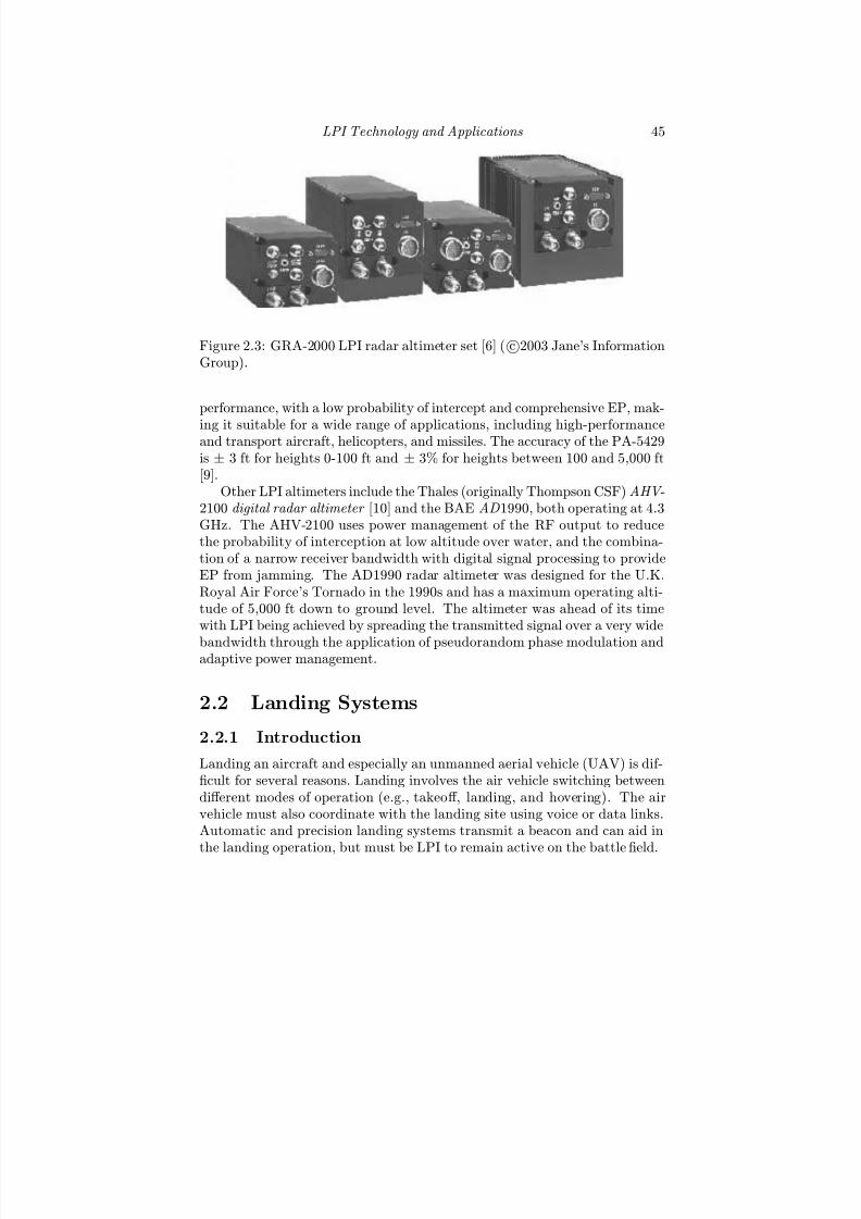
7/17/2019 1596932341 Intercept Radar.pdf
http://slidepdf.com/reader/full/1596932341-intercept-radarpdf 76/891
LPI Technology and Applications 45
Figure 2.3: GRA-2000 LPI radar altimeter set [6] ( c2003 Jane’s InformationGroup).
performance, with a low probability of intercept and comprehensive EP, mak-
ing it suitable for a wide range of applications, including high-performanceand transport aircraft, helicopters, and missiles. The accuracy of the PA-5429is ± 3 ft for heights 0-100 ft and ± 3% for heights between 100 and 5,000 ft[9].
Other LPI altimeters include the Thales (originally Thompson CSF) AHV -2100 digital radar altimeter [10] and the BAE AD 1990, both operating at 4.3GHz. The AHV-2100 uses power management of the RF output to reducethe probability of interception at low altitude over water, and the combina-tion of a narrow receiver bandwidth with digital signal processing to provideEP from jamming. The AD1990 radar altimeter was designed for the U.K.Royal Air Force’s Tornado in the 1990s and has a maximum operating alti-tude of 5,000 ft down to ground level. The altimeter was ahead of its timewith LPI being achieved by spreading the transmitted signal over a very wide
bandwidth through the application of pseudorandom phase modulation andadaptive power management.
2.2 Landing Systems
2.2.1 Introduction
Landing an aircraft and especially an unmanned aerial vehicle (UAV) is dif-ficult for several reasons. Landing involves the air vehicle switching betweendiff erent modes of operation (e.g., takeoff , landing, and hovering). The airvehicle must also coordinate with the landing site using voice or data links.Automatic and precision landing systems transmit a beacon and can aid in
the landing operation, but must be LPI to remain active on the battlefi
eld.

7/17/2019 1596932341 Intercept Radar.pdf
http://slidepdf.com/reader/full/1596932341-intercept-radarpdf 77/891
46 Detecting and Classifying LPI Radar
2.2.2 Fielded LPI Landing Systems
The AN/SPN-46 is an automatic precision approach and landing system
(PALS) for aircraft carriers and amphibious assault ships. Built by Tex-tron, the AN/SPN-46 PALSs are installed on all U.S. Navy aircraft carriers,and provide safe and reliable final approach and landing guidance for MarineCorps helicopters and AV-8B Harrier vertical and/or short takeoff and land-ing (VSTOL) attack aircraft during day/night operations and adverse weatherconditions. The PALS employs LPI technology using both an f c = 9.3 and33.2-GHz carrier frequency mainly to obtain adequate accuracy. As in manyother system examples where two bands are used, one band is used for searchwhile another higher frequency band is used for tracking. Sometimes onelower band can be used for initial tracking through weather, and a higherfrequency for more precision at short range.
The PALS employs the 9.3-GHz coherent transmitter and receiver withmonopulse tracking and Doppler processing on received signals for clutter
rejection and rain attenuation at an operating range of 15 km [11]. ThePALS is also capable of controlling up to two aircraft simultaneously in a“leapfrog” pattern, because of two dual-band radar antennas/transmitters.As each approaching aircraft being assisted by the system lands, anothercan be acquired. As of 2002, Jane’s sources were reporting the SPN-46(V)as being in service aboard the U.S. Navy aircraft carrier Enterprise (tworadar installed), the Kitty Hawk, the John F. Kennedy (two radar installed),and the Nimitz (two radar installed) class aircraft carriers. The SPN-46(V)was also noted as being a retrofit option for the U.S. Navy’s “Wasp” classamphibious assault ships [12].
The Sierra Nevada tactical automatic landing system (TALS) is an all-weather, transponder tracking radar system designed for land-based environ-ments and interoperability with any ground control station (GCS). It is anupgrade of the AN/UPN-51(V) UAV Common Automatic Recovery System(UCARS) and features a millimeter wave (MMW) K-band (35 GHz) radar. Ituses a narrow beamwidth antenna for close-range LPI acquisition in fog andrain, and an omnidirectional antenna for rollout. Due to its LPI signature,the TALS has minimal impact to the host aircraft [13]. At a range of 3.7 km,the transmit power for the airborne transponder is 100 mW with a 60% dutycycle, while the ground tracking radar transmits a maximum of 1W with a0.04% duty cycle. A photo of the TALS system is shown in Figure 2.4. Theground tracking subsystem, contained in a portable unit, locates and accu-rately tracks the airborne transponder, using high-bandwidth tracking loopsto cover touchdown and roll-out. Recovery software, proven in UCARS, per-forms air vehicle guidance and control calculations. The recovery of a UAV
using the TALS is similar to the UCARS system shown in Figure 2.5 [14].The TALS has been ordered for the AAI RQ-7A Shadow 200 tactical UAVsystem and recently underwent U.S. Army trials in 2000.

7/17/2019 1596932341 Intercept Radar.pdf
http://slidepdf.com/reader/full/1596932341-intercept-radarpdf 78/891
LPI Technology and Applications 47
Figure 2.4: The tactical automatic landing system (TALS) showing the 35-GHz antenna [13] ( c2002 Jane’s Information Group).
Figure 2.5: Steps in the recovery of a UAV using a UCARS [14] ( c2002Jane’s Information Group).

7/17/2019 1596932341 Intercept Radar.pdf
http://slidepdf.com/reader/full/1596932341-intercept-radarpdf 79/891
48 Detecting and Classifying LPI Radar
2.3 Surveillance and Fire Control Radar
2.3.1 Battlefield Awareness
On the battlefield, situational awareness and threat evaluation are achievedusing tactical surveillance radar to detect and track targets. For covert op-erations, the detection and tracking of targets should be as quiet as possible.These systems employ LPI technology to decrease the probability of passivedetection by hostile forces; that is, “to see without being seen.” The role of multimode airborne fire control radar is to provide the eyes for tactical fighteraircraft within an air dominance mission and also require LPI operation.
2.3.2 LPI Ground-Based Systems
Ericsson Microwave Systems has produced several LPI radar systems forfire control and surveillance, including the Improved Helicopter and Air-
craft/Radar Detection (HARD)-3D, the Eagle, and the Pointer. The Im-proved Hard-3D is a solid-state, 3D search and acquisition radar that hasbeen designed for use in short-range air defense systems. The ImprovedHARD features an LPI capability that is due to a low output peak powerof 240W (30W average), broadband frequency agility, low side lobes, and anarrow antenna beam [15]. The 3D capability is achieved by an electronicallyscanned beam in elevation with intelligent beam control, providing a shortreaction time after the target is detected. The elevation coverage is obtainedby steering the antenna beam to a number of fixed elevations on a pulse-to-pulse basis. Figure 2.6 shows the HARD-3D radar mounted on a Hagglundsvehicle. The elevation search pattern covers up to 35 degrees in elevationwithin two antenna revolutions. Upon target detection, the beam pattern iscontrolled so that a secondary detection will always occur in the next revolu-
tion for immediate confirmation and track initiation [15]. In a special pop-upmode, the track will start automatically after the first detection. Up to 20targets and five jammers can be tracked automatically in range, azimuth, andelevation. Instrumented ranges are 12 and 20 km.
The Ericsson Microwave Systems Eagle is a fire-control LPI radar intendedfor mobile ground and naval-based air defense systems. The equipment op-erates in the K-band (35 GHz) and is used to track low-flying targets andperform air-to-surface missile alert and closed-loop fire control. The Ka-bandwaveform provides a narrow antenna beam for low-altitude tracking at shortrange, as is required for gun fire control. The Eagle system is shown in Fig-ure 2.7 and achieves LPI operation by using a low-output peak power (20W),pulse compression, high antenna gain with extremely low side lobes [16]. Theradiation pattern and a new transmission technique claim to make it impossi-ble for escort or stand-off jammers to degrade the radar performance. It cantrack two targets simultaneously with an angular error of less than 0.2 mrad

7/17/2019 1596932341 Intercept Radar.pdf
http://slidepdf.com/reader/full/1596932341-intercept-radarpdf 80/891
LPI Technology and Applications 49
Figure 2.6: HARD-3D radar on Hagglunds vehicle [15] ( c2002 Jane’s Infor-mation Group).
Figure 2.7: Missile control and launch vehicle with the mast-mounted Eagleradar [16] ( c2003 Jane’s Information Group).

7/17/2019 1596932341 Intercept Radar.pdf
http://slidepdf.com/reader/full/1596932341-intercept-radarpdf 81/891
50 Detecting and Classifying LPI Radar
Figure 2.8: Pointer LPI radar system antenna [17] ( c2003 Jane’s InformationGroup).
at 10 km.The Ericsson Microwave Systems Pointer radar system is a short-range
LPI air surveillance 3D solid state radar system that was designed to beintegrated into short-range air defense missile systems such as the Mistral,
Stinger, and Starburst [17]. Pointer is a fully autonomous system that in-cludes an X-band radar and the antenna shown in Figure 2.8. The rangeof Pointer is typically over 20 km, and 9 to 10 km in altitude. Pointer canbe brought into action in 1 minute by a single operator. Most functions of Pointer, including track initiation, tracking, classification of fixed-wing air-craft and helicopters, threat evaluation, and data distribution via radio orwire are fully automatic. Target information can be sent to the firing unit 2or 3 seconds after the target enters the line of sight. All the missile systemoperator then has to do is to acquire, track, and engage the target [17]. ThePointer operator can be positioned a long distance from the radar, using theradar remote control laptop computer shown in Figure 2.9. The Pointer wasdesigned to increase the overall eff ectiveness of short-range air defense sys-tems by reducing target acquisition time, as well as enabling more targets to
be engaged [17]. Pointer builds on Ericsson Microwave Systems’ experiencein the development of both the HARD-3D and Eagle LPI radar.Hollandse Signaalapparaten is developing a LPI radar as an alternative

7/17/2019 1596932341 Intercept Radar.pdf
http://slidepdf.com/reader/full/1596932341-intercept-radarpdf 82/891
LPI Technology and Applications 51
Figure 2.9: Pointer operator’s radar remote control unit that is deployed awayfrom the radar unit [17] ( c2003 Jane’s Information Group).
to the use of infrared sensors for short-range missile and gun systems. Thecompany’s PAGE (portable air-defense guard equipment) is a lightweight andinexpensive 8—10 GHz (I-band) FMCW emitter with a transmit power of only10—20W, providing a detection range of 10—15 km [18]. The PAGE LPI radarsystem, shown in Figure 2.10, exploits Signaal’s experience in developing itsScout family of naval and land-based FMCW ground surveillance LPI radars.1
It is also being developed as a private venture by Thales Nederland as a low-level air surveillance radar which provides early warning and cueing data for
short-range networked air defense applications. Especially of interest are theman-portable surface-to-air missiles (SAM) and light anti-aircraft guns. ThePAGE can survive the most extreme EA conditions and is nearly undetectableby ES and radar warning receivers.
The PAGE system consists of an antenna unit including a solid-state trans-ceiver, a radar processor unit, an operator unit, and a small generator. It alsohas the capability to integrate an identification friend-or-foe (IFF). (An au-tomated datalink and weapons terminal can be added to PAGE for real-timedata processing at remote fire units). Configurations include a man-portabletripod version, a light vehicle or trailer mounting and installation on existingself-propelled anti-aircraft gun or SAM systems [18].
1The GB-Squire is a variant of the PAGE, and has detected artillery shells and Browning0.50-calibre machine gun bullets in flight during testing.

7/17/2019 1596932341 Intercept Radar.pdf
http://slidepdf.com/reader/full/1596932341-intercept-radarpdf 83/891
52 Detecting and Classifying LPI Radar
Figure 2.10: PAGE LPI radar system [18] ( c2006 Jane’s Information Group).
The Thales Nederland (formerly Signaal) Variant shown in Figure 2.11,is a dual-band (4—6 GHz and 8—10 GHz) radar (one octave apart) that is rel-atively low-cost low-power, and lightweight making it ideal for a broad rangeof vessels, including fast patrol boats, amphibious vessels and support ships[19]. It has an autonomous target detection and tracking capability and is
intended to fi
ll three principal functions. These include surface target de-tection and tracking, air target detection and tracking, and gunfire targetingsupport.
The Variant uses an integrated solid-state FMCW emitter with a transmitpower P avg = 10 mW. The antenna rotates at 14 rpm for long-range surveil-lance and at 28 rpm for a higher update rate (for self-defense applications).The system is fully coherent and provides pulse Doppler detection and track-ing algorithms for optimal clutter suppression and air targeting. Spread spec-trum techniques are used to enable detection and classification of helicopters.Surface gunfire support is provided for by three fire-control/splash-spottingwindows, eliminating the need for a dedicated tracking radar for engagementof surface targets [19]. The system is able to detect air and surface targets outto instrumented ranges of 60 km and 70 km respectively. Important features
include the ability to detect hovering and slow-moving helicopters, and a highresistance to jamming, weather clutter, and multipath propagation due to thedual-band operation and LPI operation.
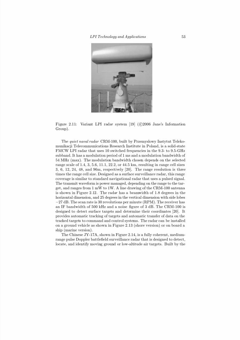
7/17/2019 1596932341 Intercept Radar.pdf
http://slidepdf.com/reader/full/1596932341-intercept-radarpdf 84/891
LPI Technology and Applications 53
Figure 2.11: Variant LPI radar system [19] ( c2006 Jane’s InformationGroup).
The quiet naval radar CRM-100, built by Przemyslowy Instytut Teleko-munikacji Telecommunications Research Institute in Poland, is a solid-stateFMCW LPI radar that uses 10 switched frequencies in the 9.3- to 9.5-GHzsubband. It has a modulation period of 1 ms and a modulation bandwidth of 54 MHz (max). The modulation bandwidth chosen depends on the selectedrange scale of 1.4, 3, 5.6, 11.1, 22.2, or 44.5 km, resulting in range cell sizes3, 6, 12, 24, 48, and 96m, respectively [20]. The range resolution is threetimes the range cell size. Designed as a surface surveillance radar, this range
coverage is similar to standard navigational radar that uses a pulsed signal.The transmit waveform is power managed, depending on the range to the tar-get, and ranges from 1 mW to 1W. A line drawing of the CRM-100 antennais shown in Figure 2.12. The radar has a beamwidth of 1.8 degrees in thehorizontal dimension, and 25 degrees in the vertical dimension with side lobes−27 dB. The scan rate is 30 revolutions per minute (RPM). The receiver hasan IF bandwidth of 500 kHz and a noise figure of 3 dB. The CRM-100 isdesigned to detect surface targets and determine their coordinates [20]. Itprovides automatic tracking of targets and automatic transfer of data on thetracked targets to command and control systems. The radar can be installedon a ground vehicle as shown in Figure 2.13 (shore version) or on board aship (marine version).
The Chinese JY-17A, shown in Figure 2.14, is a fully coherent, medium-
range pulse Doppler battlefield surveillance radar that is designed to detect,locate, and identify moving ground or low-altitude air targets. Built by the

7/17/2019 1596932341 Intercept Radar.pdf
http://slidepdf.com/reader/full/1596932341-intercept-radarpdf 85/891
54 Detecting and Classifying LPI Radar
Figure 2.12: The CRM-100 quiet naval radar antenna (measurements shownin millimeters) [20] ( c2003 Jane’s Information Group).
Figure 2.13: The CRM-100 quiet naval radar installation [20] ( c2003 Jane’sInformation Group).

7/17/2019 1596932341 Intercept Radar.pdf
http://slidepdf.com/reader/full/1596932341-intercept-radarpdf 86/891
LPI Technology and Applications 55
Figure 2.14: JY-17A medium-range ground surveillance radar [21] ( c2003Jane’s Information Group).
East China Institute of Electronic Engineering, the radar can be vehicle—mounted or ground—deployed. The radar features a solid-state, LPI trans-mitter in the 8- to 12-GHz range, and a high-stability frequency synthesizer[21]. It also has a selective linear and circular polarization antenna with lowside lobes and digital phase coding, random frequency shift keying, with pulseDoppler processing that has automatic target detection and tracking. It candetect a single pedestrian at 10 km, a light vehicle at 15 km, a helicopter at20 km, and a ship at 30 km [21].
The Raytheon multirole survivable radar (MRSR) is a tactical target ac-quisition and tracking LPI radar for the U.S. Army Missile Command to meetthe tactical air defense requirements in the high-to-medium air defense andforward-area air defense mission areas. The radar is a 3D track-while-scan,phased array in elevation radar; designed to acquire and track multiple air-borne targets over a 360-degree azimuth at extended ranges and at all tacticalaltitudes. Targets include tactical aircraft, UAVs, and hovering and slowlymoving helicopters. The LPI radar incorporates a solid-state, low noise trans-mitter, and operates over a wide bandwidth with frequency agility [22]. Theradar aperture is optimized to resist advanced EA and antiradiation missiles
by employing very low side lobes combined with the LPI waveform. Multiplebeams are moved electronically in elevation, with one continuously scanningthe horizon with its bottom edge touching the ground, producing hot spots

7/17/2019 1596932341 Intercept Radar.pdf
http://slidepdf.com/reader/full/1596932341-intercept-radarpdf 87/891
56 Detecting and Classifying LPI Radar
to confuse antiradiation missile seekers [22].
2.3.3 LPI Airborne SystemsThe AN/APS-147 multimode radar is an inverse synthetic aperture radar(ISAR) system designed to support the multimission capability of the lightairborne multipurpose (LAMPS) SH-60B helicopter system during maritimesurveillance and patrol missions. Power management and frequency agilitygive the operators the ability to perform missions at output power levels lowerthan traditional maritime surveillance radar. This enables the radar to detectmedium-to-long-range targets with an LPI capability against enemy interceptreceivers. Radar modes include target imaging, small target (periscope) de-tection, long-range surveillance, weather detection and avoidance, all-weathernavigation, short-range search and rescue, and enhanced LPI search and tar-get designation [23].
The AN/APQ-181 is the LPI radar designed specifically for the NorthropGrumman B-2 Spirit stealth bomber. The B-2 is in use by the U.S. Air Forceand is shown in Figure 2.15. The radar operates in the J-band (12.5—18 GHz),using 21 separate modes for terrain following and terrain avoidance, naviga-tion system updates, target search, location, identification and acquisition,and weapons delivery [24]. The radar employs two electronically scanned an-tennas and advanced LPI techniques that match the aircraft’s overall stealthqualities. The antenna is electronically steered in two dimensions and featuresa monopulse feed design to enable fractional beamwidth angular precision. Itis designed to have a low RCS with respect to both in- and out-of-band RFillumination [25].
The AN/APG-77 is an advanced multimode tactical radar and is the pri-mary sensor for the F-22 Raptor fighter aircraft built by Northrop Grumman
(with Raytheon). A photo of the F-22 Raptor is shown in Figure 2.16. TheLPI nature of the APG-77 radar provides a significant advantage for the F-22. The F-22 is able to detect RWR/ES-equipped fighter aircraft withoutthem knowing they are being illuminated [26]. The APG-77 emits low energypulses over a wide frequency band. That is, the emitter changes frequencyand power levels after every pulse, in order that no two transmitted pulses arealike. When multiple echoes are sent back to the radar, the signal processorconverts the signals together instead of individually. The radar antenna is afixed, elliptical, electronically scanned active array that contains 2,000 trans-mit and receive (TR) modules [27]. The antenna also contains circulators,radiators, and manifolds assembled into subarrays and then integrated into acomplete array. The active array requires significantly less volume and primepower than a gimbaled slotted array. The antenna is integrated both phys-
ically and electromagnetically with the airframe and has a low radar crosssection. The active array provides frequency agility, low radar cross section,agile beam steering, and a wide bandwidth capability typical of LPI radar.

7/17/2019 1596932341 Intercept Radar.pdf
http://slidepdf.com/reader/full/1596932341-intercept-radarpdf 88/891
LPI Technology and Applications 57
Figure 2.15: The Northrop Grumman B-2 bomber carries the Raytheon Elec-tronic Systems AN/APQ-181 radar [24] ( c2002 Jane’s Information Group).
Figure 2.16: The F-22 Raptor employs the LPI AN/APG-77 radar [27]
( c2003 Jane’s Information Group).

7/17/2019 1596932341 Intercept Radar.pdf
http://slidepdf.com/reader/full/1596932341-intercept-radarpdf 89/891
58 Detecting and Classifying LPI Radar
The low-altitude navigation and targeting infrared for night (LANTIRN) isa system consisting of two pods that allow aircrew to fly their aircraft by dayor night and in adverse meteorological conditions. The LANTIRN consists of a navigation pod and a targeting pod. The navigation pod contains a widefield of view forward looking infrared (FLIR) and a Ku-band LPI terrainfollowing radar, the AN/APN-237A, that can be linked directly to the F-16’sautopilot to automatically maintain a preset altitude down to 100 feet whileflying over virtually any kind of terrain. It has five modes: normal, weather,EP, LPI, and very low clearance [28]. The targeting pod contains anotherFLIR and a laser designator/rangefinder. The LANTIRN is deployed on theF-16C/D, F-15E/I/S, and F-14 platforms.
2.4 Antiship Capable Missile and Torpedo
Seekers
2.4.1 A Significant Threat to Surface Navies
Antiship capable missiles (ASCMs) are a significant threat to navy surfaceships. Active RF ASCM seekers that radiate substantial transmitter power,however, allow themselves to be detected by relatively modest intercept re-ceivers in both the main and side lobes. The intercept of seeker transmissionsultimately leads to vulnerability through the use of antiradiation missiles,missile interceptors, or EA. In the future, RF seekers will have LPI, power-managed operation in the 8- to 20-GHz range as well as the 35- and 96-GHzranges, by incorporating a number of advanced electronic technologies. Thesetechnologies will enable the missile to generate a broad collection of wide-band reprogrammable waveforms with bandwidths reaching 500 MHz to 1
GHz. Using a variety of wideband techniques and coherent range-Dopplerprocessing, these seekers will eff ectively target low radar cross section ships,while simultaneously allowing the seeker to escape detection and reject decoyssuch as chaff . Chapter 7 examines ASCM seeker technology and explores amissile-ship engagement scenario where the missile uses a power-managed,LPI seeker to detect a low RCS ship in several sea states.
2.4.2 Fielded LPI Seeker Systems
The Saab Bofors Dynamics AB’s RBS-15 medium-range, radar-guided, air-to-surface missile is one of a family of long-range ASCMs produced in Swedenthat can be launched from the air, land, or sea [29]. The missile makes use of low RCS materials to reduce the likelihood of early detection by enemy radar
and also has a low infrared signature to reduce the probability of detectionby infrared search and track systems. A picture of the RBS-15 is shown inFigure 2.17. In the 1990s, the company developed and tested an LPI radar

7/17/2019 1596932341 Intercept Radar.pdf
http://slidepdf.com/reader/full/1596932341-intercept-radarpdf 90/891
LPI Technology and Applications 59
Figure 2.17: RBS-15 missile.
seeker for the RBS-15 (Mk 2). The seeker uses FMCW technology and hasoutput power in the milliwatt range that is progressively reduced as the missile
approaches the target. In 1994, Saab began work on the next generationRBS-15 (Mk 3) that incorporates an updated version of the current turbojetengine, providing a range in excess of 200 km [29]. Saab is developing afuture land-attack version of the RBS-15 Mk 3 and is working on several newseeker technologies that may be applicable and that may also be retrofitted toexisting variants. These include synthetic aperture radar, which would boostseeker resolution by more than 100% and substantially increase the seeker’starget discrimination capability as well as the terminal aimpoint accuracy.Another option is an LPI radar seeker that would use long, coded pulses thatare difficult to detect and difficult to jam. Prototypes for both the syntheticaperture and LPI seekers are currently under test [29]. The improved Mk 3version uses a global positioning system (GPS) data link, and the range hasbeen increased to 400 km.
Sweden is also developing automatic target recognition (ATR) systemsthat would give the missile a better discrimination capability. One option isfor a dual-mode seeker version that combines the LPI radar with an imaginginfrared (IIR) seeker, using ATR for terminal guidance. Figure 2.18 showsthe RBS-15 missile being fired from a ground-based launch site.
Another type of LPI approach is the random noise emitter. DARPAis investigating this type of seeker for the miniature air-launched intercep-tor (MALI). The MALI is a supersonic armed version of the miniature air-launched decoy (MALD) and is used to intercept cruise missiles in flight fromthe rear. Figure 2.19 shows the MALI mounted on an aircraft ready forlaunch. The noise seeker is a Ka-band (35 GHz) seeker with 1-GHz band-width, and transmits randomly generated noise signals to detect and homein on the cruise missile. The randomly generated noise signals are copied
and stored in seeker memory in order to correlate with the radar return. Notonly does the randomness of the noise seeker make it harder for an intercept

7/17/2019 1596932341 Intercept Radar.pdf
http://slidepdf.com/reader/full/1596932341-intercept-radarpdf 91/891
60 Detecting and Classifying LPI Radar
Figure 2.18: RBS-15 missile firing.
Figure 2.19: Miniature air-launched interceptor [30] ( c2003 Aviation Weekand Space Technology).
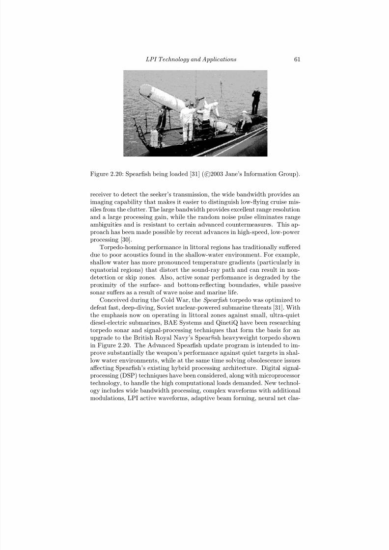
7/17/2019 1596932341 Intercept Radar.pdf
http://slidepdf.com/reader/full/1596932341-intercept-radarpdf 92/891
LPI Technology and Applications 61
Figure 2.20: Spearfish being loaded [31] ( c2003 Jane’s Information Group).
receiver to detect the seeker’s transmission, the wide bandwidth provides animaging capability that makes it easier to distinguish low-flying cruise mis-siles from the clutter. The large bandwidth provides excellent range resolutionand a large processing gain, while the random noise pulse eliminates rangeambiguities and is resistant to certain advanced countermeasures. This ap-proach has been made possible by recent advances in high-speed, low-powerprocessing [30].
Torpedo-homing performance in littoral regions has traditionally suff ereddue to poor acoustics found in the shallow-water environment. For example,shallow water has more pronounced temperature gradients (particularly inequatorial regions) that distort the sound-ray path and can result in non-detection or skip zones. Also, active sonar performance is degraded by theproximity of the surface- and bottom-reflecting boundaries, while passivesonar suff ers as a result of wave noise and marine life.
Conceived during the Cold War, the Spear fi sh torpedo was optimized todefeat fast, deep-diving, Soviet nuclear-powered submarine threats [31]. Withthe emphasis now on operating in littoral zones against small, ultra-quietdiesel-electric submarines, BAE Systems and QinetiQ have been researchingtorpedo sonar and signal-processing techniques that form the basis for anupgrade to the British Royal Navy’s Spearfish heavyweight torpedo shownin Figure 2.20. The Advanced Spearfish update program is intended to im-prove substantially the weapon’s performance against quiet targets in shal-low water environments, while at the same time solving obsolescence issuesaff ecting Spearfish’s existing hybrid processing architecture. Digital signal-processing (DSP) techniques have been considered, along with microprocessor
technology, to handle the high computational loads demanded. New technol-ogy includes wide bandwidth processing, complex waveforms with additionalmodulations, LPI active waveforms, adaptive beam forming, neural net clas-

7/17/2019 1596932341 Intercept Radar.pdf
http://slidepdf.com/reader/full/1596932341-intercept-radarpdf 93/891
62 Detecting and Classifying LPI Radar
sification, and advanced tracking [31]. Adaptive beam-forming is also used toovercome the eff ects of EA by noise jammers.
2.5 Summary of LPI Radar Systems
This chapter presented several LPI radar system applications where theirdesign intentionally (and sometimes unintentionally) makes their transmis-sion difficult to intercept. Table 2.1 summarizes the systems discussed, alongwith their application or use. It is important to note that indentifying anLPI radar as any radar system that uses higher than conventional duty cy-cles (through pulse compression or CW operation), solid state transmitters,low side-lobe antennas, or low transmitter power, can end up leading to amisclassification. For example, under this definition, the new ballistic missileearly warning system (BMEWS), Pave phased array warning system (PAWS)radar, airborne warning and control system (AWACS) radar, air route surveil-
lance radar model 4 (ARSR-4), and any police CW radar would be classifiedas LPI, which is certainly not correct. In the next few chapters, details onthe LPI technology and the important pulse compression techniques used inthe above applications are presented.

7/17/2019 1596932341 Intercept Radar.pdf
http://slidepdf.com/reader/full/1596932341-intercept-radarpdf 94/891
LPI Technology and Applications 63
Table 2.1: LPI Radar Systems
Developer System LPI Use
NavCom Defense Electronics AN/APN-232 Combined altitude radar altimeterHoneywell HG-9550 Radar altimeterNAVAIR GRA-2000 Tri-service radar altimeterTellumat, South Africa PA-5429 Radar altimeterHoneywell CMRA Cruise missile radar altimeterThompson CSF AHV-2100 Radar altimeterBAE AD1990 Radar altimeterTextron Systems AN/SPN-46 (V) Precision approach, automatic landingSierra Nevada TALS Tactical automatic landing systemSaab Bofors Pilot Surveillance, navigationSignaal Scout Surveillance, navigationSignaal Smart-L SurveillanceEricsson Microwave Systems HARD-3D Fire control and surveillanceEricsson Microwave Systems Eagle Fire controlEricsson Microwave Systems Pointer Air surveillance radarThales Nederland PAGE Air surveillanceThales Nederland Variant Surface and air target, gun fire detectionPITT Research Institute, Poland CRM-100 Surface target detectionChina Inst. of Elec. Engineering JY-17A Battlefield surveillance radarRaytheon MRSR Target acquisition and tracking radarTI AN/APS-147 Enhanced search and target designationRaytheon AN/APQ-181 Tactical multimode fire control radarNorthrop Grumman AN/APG-77 Multimo de tactical radarRaytheon AN/APG-70 Multimode tactical radarTI LANTIRN Terrain following radarSaab Dynamics RBS-15MR Radar guided air-to-surface missileBAE Spearfish Torpedo for littoral environments
7/17/2019 1596932341 Intercept Radar.pdf
http://slidepdf.com/reader/full/1596932341-intercept-radarpdf 95/891
64 Detecting and Classifying LPI Radar
References
[1] “AN/APN-232 combined altitude radar altimeter,” Jane’s Avionics - Military
CNS, FMS, Data and Threat Management , Feb. 10, 2003.[2] http://www.osmpf.wpafb.af.mil/.
[3] “Lockheed Martin Aeronautics Company,” Jane’s All the Worlds Aircraft-Fixed Wing-Military , Jan. 10, 2003.
[4] “HG9550 LPI radar altimeter system,” Jane’s Avionics - Military CNS, FMS,Data and Threat Management , April 26, 2002.
[5] “Cruise missile radar altimeter,” Jane’s Radar , July 17, 1994.
[6] “AN/APN-209 radar altimeter,” Jane’s Avionics - Military CNS, FMS, Data and Threat Management , Feb. 10, 2003.
[7] “GRA-2000 low probability of intercept (LPI) altimeter,” Jane’s Avionics -Military CNS, FMS, Data and Threat Management , Feb. 5, 2003.
[8] http://www.cni.na.baesystems.com/html/low probability of intercept a.html
[9] “PA-5429 radar altimeter,” Jane’s Avionics - Military CNS, FMS, Data and Threat Management , Feb. 5, 2003.
[10] “AHV-2100 digital radar altimeter,” Jane’s Avionics - Military CNS, FMS,Data and Threat Management , Feb. 10, 2003.
[11] http://www.fas.org/man/dod-101/sys/ship/weaps/an-spn-46.htm.
[12] “AN/SPN-46(V) approach radar,” Jane’s Radar and Electronic Warfare Sys-tems, Military Air Tra ffi c Control, Instrumentation and Ranging Radars , Feb.7, 2003.
[13] “Sierra Nevada TALS,” Jane’s Unmanned Aerial Vehicles and Targets - Launch and Recovery Systems, April 17, 2002.
[14] “Sierra Nevada UCARS,” Jane’s Unmanned Aerial Vehicles and Targets -Launch and Recovery Systems, April 17, 2002.
[15] “Ericsson Microwave Systems Improved HARD-3D radar system,” Jane’s Land-Based Air Defence-Anti-Aircraft Control Systems , Oct. 23, 2002.
[16] “Eagle fire-control radar,” Jane’s Radar and Electronic Warfare Systems,Battle fi eld, Missile Control and Ground Surveillance Radar Systems, Jan.30, 2003.
[17] “Ericsson Microwave Systems Pointer radar system,” Jane’s Land-Based Air Defence-Anti-Aircraft Control Systems , 1999.
[18] Hewish, M., “Low-level air defense—new sensors enhance eff ectiveness,” Jane’s Defence Equipment and Technology , Vol. 27, No. 6, pp. 43, June, 1994.
[19] “Aff ordable performers: surveillance radars balance cost with capability,”International Defence Review , Mar., 2008.
[20] “CRM-100 surveillance radar,” Jane’s Radar and Electronic Warfare Systems-
Naval/Coastal Surveillance and Navigation Radar , Jan. 30, 2003.[21] “JY-17 battlefield reconnaissance radar,” Jane’s C4I Systems-Land Based
Surveillance and Location , April, 22, 2002.

7/17/2019 1596932341 Intercept Radar.pdf
http://slidepdf.com/reader/full/1596932341-intercept-radarpdf 96/891
LPI Technology and Applications 65
[22] “Multi-role survivable radar - Tactical target acquisition and tracking,” Jane’s Air Defence Radar - Land and Sea , Jan. 1997.
[23] “AN/APS-147 multimode airborne radar,” Jane’s Avionics - Military CNS,FMS, Data and Threat Management , Feb. 10, 2003.
[24] “AN/APQ-181 radar for the B-2,” Jane’s Avionics - Military CNS, FMS,Data and Threat Management , Jan. 17, 2003.
[25] http://www.raytheon.com/products/apq181/.
[26] http://f22rap.virtualave.net/avionics.html.
[27] “AN/APG-77 multimode airborne radar,” Jane’s Radar and Electronic War- fare Systems-Airborne Fire Control Radar , Nov. 11, 2002.
[28] http://www.f-16.net/reference/armament/lantirn.html.
[29] “RBS 15F,” Jane’s Air-Launched Weapons-Air to Surface Missiles, Sept. 12,2002.
[30] R. Wall, “USAF eyes decoy, jammer as MALI demonstration ends,” Aviation
Week and Space Technology , Jan. 13, 2003.
[31] “Spearfish,” Jane’s Underwater Warfare Systems - Torpedos , May 3, 2002.
Problems
1. In an FMCW altimeter such as the CARA, the frequency is sweptover the modulation bandwidth ∆F during the modulation (coherentprocessing) period tm. Ranging (determining the altitude) occurs bymixing a sample of the transmitted signal with the reflected signal fromthe surface to derive a diff erence frequency (or beat frequency) δ f . (a)Write an expression for the time interval that corresponds to the mea-sured beat frequency δ f as a function of the sweep rate ∆F . (b) Deter-
mine the beat frequency (in Hz) for the CARA if the modulation periodis 1 ms and the altimeter is at a height of 30m. HINT: the wavefronttakes 6.7 μs/km to travel a round-trip path.
2. Estimate the maximum intercept range of the TALS ground trackingradar if its MMW antenna is 60% efficient and the intercept receiversensitivity is δ I = −100 dBmi.
3. Estimate the HARD-3D pulse width τ R if the maximum unambiguousrange is 20 km.
4. Determine the maximum detection range of the Eagle radar, consideringthat the antenna is 90% efficient.

7/17/2019 1596932341 Intercept Radar.pdf
http://slidepdf.com/reader/full/1596932341-intercept-radarpdf 97/891

7/17/2019 1596932341 Intercept Radar.pdf
http://slidepdf.com/reader/full/1596932341-intercept-radarpdf 98/891
Chapter 3
Ambiguity Analysis of LPI
Waveforms
In this chapter, the ambiguity (delay-Doppler) analysis of LPI waveforms isaddressed. Ambiguity analysis is important to understand the properties of the CW waveform and its eff ect on measurement accuracy, target resolution,ambiguities in range, and radial velocity, and its response to clutter. Theperiodic autocorrelation function (PACF) is introduced, and it is shown thatCW signals can have a perfect PACF with zero side lobes. The periodic
ambiguity function (PAF) is also introduced, to analyze the response of amatched receiver that uses N copies of the reference (transmitted) function tocross-correlate the return CW signal and perform target detection. The PAFis similar to the ambiguity function often used to represent the magnitude of the matched receiver output for a coherent pulse train. The cut of the PAF
at zero Doppler (ν = 0) is the PACF, and cuts of the PAF along zero delay(τ = 0) yield the response of the correlation receiver at a given Doppler shift.Several important properties of the PAF are presented.
The MATLAB low probability of intercept toolbox (LPIT) is described(Appendix A) and is used to generate a CW Frank signal in order to demon-strate the PACF and PAF concepts. The MATLAB code used to calculatethe PACF and PAF is also described (Appendix B). Modifying the referencewaveform in the receiver with a weighting function (mismatched receiver) canhelp reduce the Doppler side lobes that appear. This subject is addressed,and three important weighting functions are presented.
67

7/17/2019 1596932341 Intercept Radar.pdf
http://slidepdf.com/reader/full/1596932341-intercept-radarpdf 99/891
68 Detecting and Classifying LPI Radar
3.1 The Ambiguity Function
A matched radar receiver performs a cross-correlation of the received signal
and a reference signal, whose envelope is the complex conjugate of the enve-lope of the transmitted signal. The ambiguity function describes the responseof this matched receiver to a finite duration signal. In ambiguity analysis,the receiver is considered matched to a target signal at a given delay andtransmitted frequency. The ambiguity is then a function of any added delayand additional Doppler shift from what the receiver was matched to. If u(t)is the complex envelope of both the transmitted signal and received signal,the ambiguity function is given by [1]
|χ(τ , ν )| =
∞
−∞
u(t)u∗(t − τ )ej2πν tdt
(3.1)
where τ is the time delay and ν is the Doppler frequency shift. The 3D plot,
as a function of τ and ν , is called the ambiguity diagram. The maximum of the ambiguity function occurs at the origin (τ = 0, ν = 0), and |χ(0, 0)| isthe output if the target appears at the delay and Doppler shift for which thefilter was matched. The delay-Doppler response of the matched filter output isimportant for understanding the properties of the radar waveform [2]. Ideally,the ambiguity diagram would consist of a diagonal ridge centered at the origin,and zero elsewhere (no ambiguities). The ideal ambiguity function, however,is impossible to obtain. For a coherent pulse train consisting of N R pulses withpulse duration τ R and pulse repetition interval T r, the ambiguity functionindicates that the Doppler resolution is the inverse of the total duration of the signal N RT r while the delay resolution is the pulse duration [3].
3.2 Periodic Autocorrelation FunctionLPI signals are typically low-power CW waveforms that are modulated by aperiodic function, such as a phase code sequence or linear frequency ramp. Amajor advantage of the periodically modulated CW waveforms is that theycan yield a perfect PACF. For example, consider a phase-coded CW signalwith N c phase codes each with subcode duration tb s. The transmitted CWsignal has a code period T = N ctb s and a periodic complex envelope u(t)given as
u(t) = u(t + nT ) (3.2)
for n = 0,±1, ±2, ±3 . . . . The values of the PACF as a function of the delayr (which are multiples of tb) are given by
R(rtb) = 1
N c
N cn=1
u(n)u∗(n + r) (3.3)

7/17/2019 1596932341 Intercept Radar.pdf
http://slidepdf.com/reader/full/1596932341-intercept-radarpdf 100/891
Ambiguity Analysis of LPI Waveforms 69
and ideally we would like a perfect PACF or
R(rtb) = 1, r = 0(modN c)
0, r = 0(modN c) (3.4)
Since the CW signal is continuous, the perfect PACF is possible. Note how-ever, that finite duration signals, such as a pulse train, cannot achieve thisideal autocorrelation since as the first sample (or last sample) enters (orleaves) the correlator, there is no sample that can cancel the product to yielda zero output.
3.3 Periodic Ambiguity Function
The periodic ambiguity function or PAF, introduced by Levanon and Freed-man [4], describes the response of a correlation receiver to a CW signal mod-
ulated by a periodic waveform with period T , when the reference signal isconstructed from an integral number N of periods of the transmitted signal(coherent processor length NT ). The target illumination time (dwell time)P T must be longer than N T (see Figure 1.9). As long as the delay τ isshorter than the diff erence between the dwell time and the length of the ref-erence signal 0 ≤ τ ≤ (P − N )T , the illumination time can be consideredinfinitely long and the receiver response can be described by the PAF givenas [5]
|χNT (τ , ν )| =
1
N T
NT
0
u (t − τ ) u∗ (t) ej2πν tdt
(3.5)
where τ is assumed to be a constant, and the delay rate of change is rep-resented by the Doppler shift ν . The PAF for N periods is related to the
single-period ambiguity function by a universal relationship
|χNT (τ , ν )| = |χT (τ , ν )|
sin(N πν T )
N sin(πν T )
(3.6)
where
|χT (τ , ν )| = 1
T
T 0
u(t − τ )u∗(t)ej2πν tdt
(3.7)
is the single period ambiguity function. The single period ambiguity functionis multiplied by a universal function of N and T that is independent of thecomplex envelope of the signal and that does not change with τ . The PAFshows the eff ect of using a reference receiver consisting of N code periods (seeSection 1.3). Examination of (3.6) reveals that for a large number of code
periods N , the PAF is increasingly attenuated for all values of ν except atmultiples of 1/T . It also has main lobes at ν T = 0, ±1,±2, . . . . Equation(3.6) also reveals that the PAF has relatively strong Doppler side lobes.
7/17/2019 1596932341 Intercept Radar.pdf
http://slidepdf.com/reader/full/1596932341-intercept-radarpdf 101/891
70 Detecting and Classifying LPI Radar
The PAF serves CW radar signals in a similar role to which the traditionalambiguity function serves finite duration signals. Note that for a large N , thePAF is compressed to zero for all ν , except near ν = n/T, n = 0, ±1,±2, . . . .For an infinitely large N , the function |χNT (τ , ν )| becomes a train of impulses.For large N , the PAF of a sequence exhibiting perfect periodic autocorrelationwill strongly resemble the ambiguity function of a coherent pulse train.
3.3.1 Periodicity of the PAF
The PAF formulation given in (3.5) is not unique, and alternate definitionshave also been adopted [6]. The form of the PAF in (3.5), however, representsthe straightforward implementation of a matched filter to the signal u(t)delayed by τ and Doppler shifted by ν . It can easily be shown that the cutalong the PAF’s delay axis |χNT (τ , 0)| (zero Doppler) is the magnitude of thePACF of the signal given by (3.3) [4, 6]. The cut along the Doppler axis (zerodelay) is
χNT (0, ν ) = 1
N T
NT
0
|u(t)|2ej2πν tdt (3.8)
Assuming a constant amplitude signal, |u(t)| = 1 (e.g., phase-modulated CWsignals)
|χNT (0, ν )| =
sin(πν N T )
πν N T
(3.9)
and|χNT (0, 0)| = 1 (3.10)
For any integer n, the periodicity on the delay axis is
|χNT (nT, ν )| = |χNT (0, ν )| (3.11)
For the ν axis, for m = 0,±1,±2, . . .
|χNT (τ ,m/T )| = |χNT (τ + nT, m/T )| (3.12)
The symmetry cuts are a function of the three parameters: the code periodT , the number of phase codes N c, and the number of code periods used inthe correlation receiver N . Additional symmetry and periodicity propertiesare discussed in [4, 6].
3.3.2 Peak and Integrated Side Lobe Levels
The time side lobe levels in the autocorrelation function (ACF) help quantify
the LPI waveform in its ability to detect targets without interfering side lobetargets. That is, if the ACF has high side lobes, a second nearby targetmight be able to hide in a side lobe and go undetected. To quantify the LPI
7/17/2019 1596932341 Intercept Radar.pdf
http://slidepdf.com/reader/full/1596932341-intercept-radarpdf 102/891
Ambiguity Analysis of LPI Waveforms 71
waveform characteristics, the peak side lobe level (PSL) of the ACF can bedefined as
PSL = 10log10
max side lobe power(peak response)2
= 10 log
max R
2
(k)R2(0)
(3.13)
where k is the index for the points in the ACF, R(k) is ACF for all of theoutput range side lobes except that at k = 0, and R(0) is the peak of theACF at k = 0. The integrated side lobe level is
ISL = 10 log10
total power in side lobes
(peak response)2
= 10 log
M k=−M
R2(k)
R2(0) (3.14)
and is a measure of the total power in the side lobes as compared with thecompressed peak. The PSL is a useful measure when a single point targetresponse is of concern. Values for the PSL depend on the number of subcodes
in the code sequence N c as well as the number of code periods N within thereceiver. The ISL is considered a more useful measure than the PSL whendistributed targets are of concern. Typical matched filter ISL values rangefrom −10 to −20 dB.
3.4 Frank Phase Modulation Example
To demonstrate the properties of the ACF, PACF, and PAF, we look brieflyat one important type of phase modulation called the Frank code [7]. TheFrank code is a polyphase code (more than two phase states). It has a variablelength and can be used to phase modulate a complex signal every subcodeperiod tb.
3.4.1 Transmitted Waveform
The transmitted signal can be written as
s(t) =
Ae(j2πf ct+φk)
(3.15)
where f c is the carrier frequency and φk is the phase modulation that isused to shift the phase of the carrier in time every subcode period accordingto the particular phase modulation used. Note that the carrier frequencyremains constant. The Frank phase modulation code is derived from a stepapproximation to a linear frequency modulation waveform using M frequencysteps and M samples per frequency. If i is the number of the sample in agiven frequency and j is the number of the frequency, the phase of the ith
sample of the j th frequency for the Frank code is
φi,j = 2π
M (i − 1) ( j − 1) (3.16)

7/17/2019 1596932341 Intercept Radar.pdf
http://slidepdf.com/reader/full/1596932341-intercept-radarpdf 103/891
72 Detecting and Classifying LPI Radar
Figure 3.1: Frank phase modulation for M = 8 (N c = 64).
where i = 1, 2, . . . , M , and j = 1, 2, . . . , M . The Frank code has a length
of N c = M 2 subcodes, which is also the corresponding pulse compressionratio or processing gain P GR. For tb s (the subcode period), if cpp representsthe number of carrier cycles per subcode, then tb = cpp/f c s resulting in atransmitted signal bandwidth B = 1/tb = f c/cpp. The code period can alsobe expressed as
T = N ctb = M 2tb (3.17)
Below we examine the ACF, PACF, and PAF properties of this signal. Chap-ter 5 discusses the Frank code in more detail.
3.4.2 Simulation Results
A signal containing the Frank phase modulation can easily be generated withthe MATLAB low probability of intercept toolbox distributed on the enclosedCD and described in Appendix A. The LPIT can also generate a host of otherLPI signals discussed in Chapters 4—7.
Figure 3.1 shows the Frank phase modulation (3.16) with M = 8
(N c = 64). The plot is generated within the LPIT. The carrier frequencyis f c = 1 kHz, f s = 7 kHz, and cpp = 1. Figure 3.2 shows the power spectral

7/17/2019 1596932341 Intercept Radar.pdf
http://slidepdf.com/reader/full/1596932341-intercept-radarpdf 104/891
Ambiguity Analysis of LPI Waveforms 73
Figure 3.2: Power spectral density for Frank phase modulation for M = 8(N c = 64) with f c = 1 kHz, f s = 7 kHz, and cpp = 1.
density of the Frank signal. This plot is also generated within the LPIT. Notethat since the cpp = 1, the 3-dB bandwidth B = 1 kHz, as illustrated.
The ACF and PACF are shown in Figure 3.3 for the number of codeperiods N = 1. These results can be obtained by using the output waveformsfrom the LPIT in conjuction with Levanon’s ambfn7.m code as describedin Appendix B with r = 1, F ∗ M tb = 10, T = 1, N = K = 100. ThePSL can be read from Figure 3.3(a). The largest side lobe level is 28 dBdown from the peak. This is in agreement with the theoretical result PSL =20log10(1/M π) = −28 dB (voltage ratio). Also note from Figure 3.3(b) thatthe CW Frank signal has a perfect PACF (zero side lobes). The PAF forN = 1 is shown in Figure 3.4. The phase modulation signals generatedusing the LPIT contain
bsc = cppf s
f c(3.18)
number of samples per subcode. The total number of samples within a codeperiod is then N cbsc. When ambfn7.m is used to examine the signals fromthe LPIT, the delay axis is normalized by the subcode period tb and so thePAF repeats at N cbsc since the waveform is sampled. That is, dividing this
axis by the number of samples per subcode bsc gives the delay axis in termsof the subcode number. For the LPIT default Frank signal (cpp = 1, f s = 7kHz, f c = 1 kHz), bsc = 7 and, as illustrated in the plot, the code repeats

7/17/2019 1596932341 Intercept Radar.pdf
http://slidepdf.com/reader/full/1596932341-intercept-radarpdf 105/891
74 Detecting and Classifying LPI Radar
Figure 3.3: Frank (a) ACF (PSL = −28 dB down) and (b) PACF for M = 8(N c = 64), cpp = 1 with number of reference waveforms N = 1.
Figure 3.4: PAF for Frank phase modulation for M = 8 (N c = 64), cpp = 1with number of reference waveforms N = 1.

7/17/2019 1596932341 Intercept Radar.pdf
http://slidepdf.com/reader/full/1596932341-intercept-radarpdf 106/891
Ambiguity Analysis of LPI Waveforms 75
Figure 3.5: Frank (a) ACF (PSL = −40 dB down) and (b) PACF for M = 8(N c = 64), cpp = 1 with number of reference waveforms N = 4.
every τ = 448/bsc = 64 = N c. The Doppler axis is normalized with respect tothe entire signal duration N ctb. Therefore, depending on the number of codeperiods N integrated into the PAF calculation, the Doppler lobes appear atkN for k ∈ 0, 1, 2, . . . as illustrated in Figure 3.4 for N = 1.
Increasing the number of code periods N used in the receiver can help todecrease the Doppler side lobes as well as the time side lobes in the ACF.Figure 3.5 shows the ACF and PACF for when N = 4 code periods are used
within the reference receiver (r = 1, F ∗ M tb = 40, T = 0.3, N = K = 100).Including N in the estimation of the peak side lobe level
PSL = 20 log10
1
N M π
dB (3.19)
Using N = 4, PSL = −40 dB down from the peak as shown in Figure 3.5.Figure 3.6 shows the PAF for the Frank code with N = 4 and demon-
strates that by using more copies of the reference signal within the correlationreceiver, the delay-Doppler side lobe performance improves.
3.5 Reducing the Doppler Side Lobes
To reduce the Doppler side lobes it is necessary to modify the reference signalwith a weighting function w(t) that converts the receiver from a matchedreceiver to a mismatched receiver (with a corresponding degradation in SNR

7/17/2019 1596932341 Intercept Radar.pdf
http://slidepdf.com/reader/full/1596932341-intercept-radarpdf 107/891
76 Detecting and Classifying LPI Radar
Figure 3.6: PAF for Frank phase modulation for M = 8 (N c = 64), cpp = 1with number of reference waveforms N = 4.
and decrease in resolution). Following the development in [5], the referencesignal u∗(t) in (3.5) is divided into a product of two signals: r(t) whichis periodic with the same period as u(t), and w(t) an aperiodic weightingfunction. That is, u∗(t) = r(t)w(t). The delay-Doppler response of themismatched receiver is
|ψ(τ , ν )| =
∞
−∞
u(t − τ )r(t) p(t)w(t)ej2πν tdt
(3.20)
where p(t) is an aperiodic rectangular window function
p(t) =
1 0 ≤ t < NT 0 elsewhere
(3.21)
Since (3.20) is the Fourier transform of two products (except for the miss-ing negative sign in the exponential) it can be described by the convolution(denoted ⊗) of two Fourier transforms as
|ψ(τ , ν )| = ∞
−∞
u(t − τ )r(t)ej2πν tdt
⊗
∞
−∞
p(t)w(t)ej2πν tdt
(3.22)
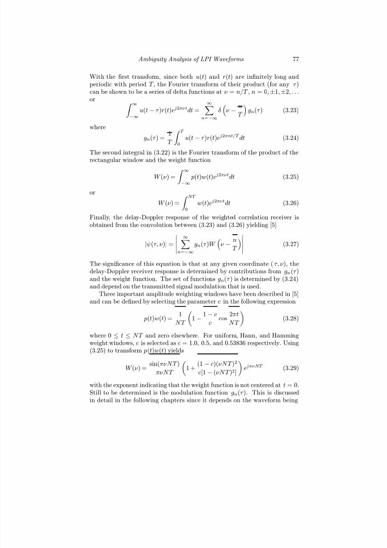
7/17/2019 1596932341 Intercept Radar.pdf
http://slidepdf.com/reader/full/1596932341-intercept-radarpdf 108/891
Ambiguity Analysis of LPI Waveforms 77
With the first transform, since both u(t) and r(t) are infinitely long andperiodic with period T , the Fourier transform of their product (for any τ )can be shown to be a series of delta functions at ν = n/T , n = 0,±1, ±2, . . .or
∞
−∞
u(t− τ )r(t)ej2πν tdt =∞
n=−∞
δ
ν − n
T
gn(τ ) (3.23)
where
gn(τ ) = 1
T
T 0
u(t − τ )r(t)ej2πnt/T dt (3.24)
The second integral in (3.22) is the Fourier transform of the product of therectangular window and the weight function
W (ν ) =
∞
−∞
p(t)w(t)ej2πν tdt (3.25)
or
W (ν ) =
NT
0
w(t)ej2πν tdt (3.26)
Finally, the delay-Doppler response of the weighted correlation receiver isobtained from the convolution between (3.23) and (3.26) yielding [5]
|ψ(τ , ν )| =
∞
n=−∞
gn(τ )W
ν − n
T
(3.27)
The significance of this equation is that at any given coordinate ( τ , ν ), thedelay-Doppler receiver response is determined by contributions from gn(τ )and the weight function. The set of functions gn(τ ) is determined by (3.24)
and depend on the transmitted signal modulation that is used.Three important amplitude weighting windows have been described in [5]and can be defined by selecting the parameter c in the following expression
p(t)w(t) = 1
N T
1 −
1 − c
c cos
2πt
N T
(3.28)
where 0 ≤ t ≤ N T and zero elsewhere. For uniform, Hann, and Hammingweight windows, c is selected as c = 1.0, 0.5, and 0.53836 respectively. Using(3.25) to transform p(t)w(t) yields
W (ν ) = sin(πν N T )
πν N T
1 +
(1 − c)(ν N T )2
c[1 − (ν N T )2]
ejπν NT (3.29)
with the exponent indicating that the weight function is not centered at t = 0.Still to be determined is the modulation function gn(τ ). This is discussedin detail in the following chapters since it depends on the waveform being

7/17/2019 1596932341 Intercept Radar.pdf
http://slidepdf.com/reader/full/1596932341-intercept-radarpdf 109/891
78 Detecting and Classifying LPI Radar
considered. Note that a smooth weight, covering N periods of the signal,aff ects only the Doppler behavior. It has no influence on the PACF (the zeroDoppler cut of the PAF). In phase-coded signals, the delay response remainsa triangle with base 2tb, regardless of any amplitude taper along N periodsof the signal.
References
[1] Levanon, N., Radar Principles , John Wiley & Sons, New York, 1988.
[2] Skolnik, M., Introduction to Radar Systems, 3rd Edition , McGraw Hill, Boston,p. 331, 2001.
[3] Levanon, N., “CW alternatives to the coherent pulse train - signals andprocessors,” IEEE Trans. on Aerospace and Electronic Systems , Vol. 29,No. 1, pp. 250—254, Jan. 1993.
[4] Levanon, N. and Freedman, A. “Periodic ambiguity function of CW signalswith perfect periodic autocorrelation,” IEEE Trans. on Aerospace and Elec-
tronic Systems , Vol. 28, No. 2, pp. 387—395, April 1992.
[5] Getz, B. and Levanon, N., “Weight eff ects on the periodic ambiguity func-tion,” IEEE Trans. on Aerospace and Electronic Systems , Vol. 31, No. 1,pp. 182—193, Jan. 1995.
[6] Freedman, A. and Levanon, N., “Properties of the periodic ambiguity func-tion,” IEEE Trans. on Aerospace and Electronic Systems , Vol. 30, No. 3,pp. 938—941, July 1994.
[7] Frank, R. L., “Polyphase codes with good nonperiodic correlation properties,”IEEE Trans. IT-9, pp. 43—45, 1963.
Problems1. When the reference signal is of duration N T , the response of the corre-
lation receiver is the PAF for N periods. Another form of the PAF canbe defined by the relationship
χNT (τ , ν ) = 1
N T
NT
0
u
t + τ
2
u∗
t − τ
2
ej2πν tdt
Starting from here, show the universal result
|χNT (τ , ν )| = |χT (τ , ν )|
sin(πν N T )
N sin(πν T )
Hint: Split the integral into N sections and use the transformation of variables t = t + (n − 1)T .

7/17/2019 1596932341 Intercept Radar.pdf
http://slidepdf.com/reader/full/1596932341-intercept-radarpdf 110/891
Ambiguity Analysis of LPI Waveforms 79
2. The complex envelope of a signal with periodic phase modulation canbe expressed as
u(t) =
N cn=1
un(t− (n − 1)tb)
where 0 ≤ t ≤ N ctb andun(t) = ejφn
for 0 ≤ t < tb. There are periodic two-valued phase sequences that canalso yield a perfect periodic autocorrelation. That is, φn = 0 or φn = φ
and un can either be 1 or β where
β = ejφ
For N c = 7,φn = 0 0 0 φ φ 0 φ
and
φ = cos−1(−3/4)
For N c = 11,φn = 0 0 0 φ φ φ 0 φ φ 0 φ
andφ = cos−1(−5/6)
For both the N c = 7 and N c = 11 sequences, (a) generate the complexCW signal using beta.m. Save the phase shift plot showing the N c phasevalues being used within a code period. (b) For the signal only, plotthe PACF and PAF (delay versus Doppler) when N = 1 and N = 4 toverify the periodicity (how often the ambiguity function repeats itself)and the reduction of the PSL. (c) Add the beta.m signal to your LPITmenu.
3. Plot the weighting function (3.29) for (a) a uniform window, (b) a Hannwindow, and (c) a Hamming window, for N = 1 and N = 5 for a codeperiod T = 0.021s (consistent with a CW LPI waveform with f c = 1kHz, M = 7, and cpp = 3).
4. Using the LPIT, generate the Frank signal with M = 8, f c = 1 kHz,f s = 7 kHz, and cpp = 1. Plot the ACF, PACF, and PAF for N = 8,and compare your results with Figures 3.5 and 3.6.
5. A phase code signal is generated with a carrier of f c = 5 kHz. Theprocessing gain of the signal is 24 dB and the bandwidth of the signalis B = 1.25 kHz. Determine (a) the subcode period tb and (b) the codeperiod T in s. (c) If the signal is intercepted with a receiver that hasan ADC with f s = 25 kHz, how many samples are within a subcodeperiod (bsc)?

7/17/2019 1596932341 Intercept Radar.pdf
http://slidepdf.com/reader/full/1596932341-intercept-radarpdf 111/891
7/17/2019 1596932341 Intercept Radar.pdf
http://slidepdf.com/reader/full/1596932341-intercept-radarpdf 112/891
Chapter 4
FMCW Radar
This chapter examines the advantages of the frequency modulation CW LPI
technique, gives detailed expressions for the transmitted signal and the re-ceived signal, and discusses the isolation required when using a single antenna.LPI search and track mode processing are discussed, and several FMCW emit-ter configurations are presented. Also investigated are the eff ects of frequencymodulation nonlinearities. Moving target indication filtering is discussed, aswell as the FMCW periodic ambiguity function. The experimental PAN-DORA multifrequency FMCW radar is presented as an example of FMCWtechnology. Electronic attack considerations are also addressed. Finally, thetechnology trends for FMCW emitters are examined.
4.1 Advantages of FMCW
CW radars that use unmodulated waveforms cannot measure a target’s range.To measure the target’s range and/or speed, the transmit frequency mustbe varied in time, and the frequency of the return signal from the targetmeasured. Correlation of the return signal with the transmit signal can givea measure of both the range and Doppler information of the target. Since themodulation cannot be continually changed in one direction (e.g., up or down),a periodic modulation is normally used. Frequency modulation can create awideband LPI waveform and take many forms, with sinusoidal and linearmodulation being used most frequently. The most popular linear modulationutilized is the triangular FMCW emitter, since it can measure the target’srange and range rate.1
1Sinusoidal frequency modulation is mathematically more tractable than linear fre-quency modulation and is presented well in [1].
81

7/17/2019 1596932341 Intercept Radar.pdf
http://slidepdf.com/reader/full/1596932341-intercept-radarpdf 113/891
82 Detecting and Classifying LPI Radar
FMCW is an eff ective LPI technique for many reasons. In some appli-cations, such as radio altimeters, a key advantage is the simple architecture,which is capable of giving a very high range resolution. Due to the verylow energy transmitted (low radiation hazard), the noncooperative interceptreceiver’s interception range is significantly reduced. This means that anFMCW radar may be used in otherwise restrictive emission-control (EM-CON) conditions that would preclude the operation of pulsed emitters. Thefrequency modulation spreads the transmitted energy over a large modulationbandwidth ∆F , providing good range resolution that is critical for discrim-inating targets from clutter. The power spectrum of the FMCW signal isnearly rectangular over the modulation bandwidth, so noncooperative inter-ception is difficult. Since the transmit waveform is deterministic, the formof the return signals can be predicted. This gives it the added advantage of being resistant to interference (such as jamming), since any signal not match-ing this form can be suppressed. Consequently, it is a difficult matter for
a noncooperative receiver to detect the FMCW waveform and measure theparameters accurately enough to match the jammer waveform to the radarwaveform (a subject we take up in Part II).
FMCW modulation is also readily compatible with solid-state transmit-ters, and represents the best use of output power available from these solidstate devices. The return signal is correlated with the transmitted signal, andis often done using analog techniques. The correlation receiver can also beimplemented using digital techniques. The frequency processing performedto obtain the range information from the digitized IF signals can be done veryquickly with FFTs. The ease with which the range resolution can be changed,and the way in which very high range resolutions can be obtained withoutrequiring wide IF and video bandwidths is also a significant advantage. Thatis, the IF and video bandwidths can be matched to the required data rate
rather than to the RF bandwidth required to give the range resolution [2].Due to the fourth power relationship between a radar’s return signal power
and the target’s range, an adequate amount of sensitivity time control (STC)must be used in the receiver to selectively attenuate the returns from close-in targets in order to control the dynamic range and prevent saturation [3].Due to the frequency-range relationship in the FMCW radar, this techniquemay be easily implemented in the frequency domain early on in the signalprocessing. FMCW is also easier to implement than phase code modulation,as long as there is no strict demand on linearity specifications over the mod-ulation bandwidth. The ability to use weighting to control the range andDoppler side lobes (mismatched correlation receiver) also allows for efficientuse of the spectrum. Finally, the advanced transceiver design allows FMCWradars to be connected to, and operated in parallel with, any available pulsed
I-band navigation radar using a common antenna. This means that the verypresence of the LPI radar cannot be ascertained by external observation.

7/17/2019 1596932341 Intercept Radar.pdf
http://slidepdf.com/reader/full/1596932341-intercept-radarpdf 114/891
FMCW Radar 83
Figure 4.1: Block diagram of a homodyne triangular FMCW radar.
4.2 Single Antenna LPI Radar for Target
Detection
A block diagram of a homodyne triangular FMCW emitter is shown in Fig-ure 4.1. In this search mode con fi guration , both the target range and Doppler
information can be measured unambiguously, while maintaining a low proba-bility of intercept. The system uses a single antenna. A triangular waveformgenerator is used to modulate the CW source for transmission. For low powersingle antenna systems, a circulator can be used to allow simultaneous trans-mission and reception [4]. With higher power systems, the transmitter noiseside bands can hide valid targets and desensitize the receiver. In this case,separate transmit and receive antennas must be used.
To enable the FMCW emitter to operate more efficiently using a single an-tenna for both transmission and reception, a reflected power canceler (RPC)is shown [3, 5]. The RPC adaptively cancels the transmit/receive feedthroughthat can limit the dynamic range of single antenna CW radar. In the case of a linear ramp, a simple RPC can adapt during the sweep to handle a widemodulation bandwidth, since the instantaneous bandwidth is small.
The target echo is received through the antenna and consists of a delayedreplica of the transmitted waveform. The instantaneous frequency diff erencebetween the received signal and the transmitted signal is a constant propor-
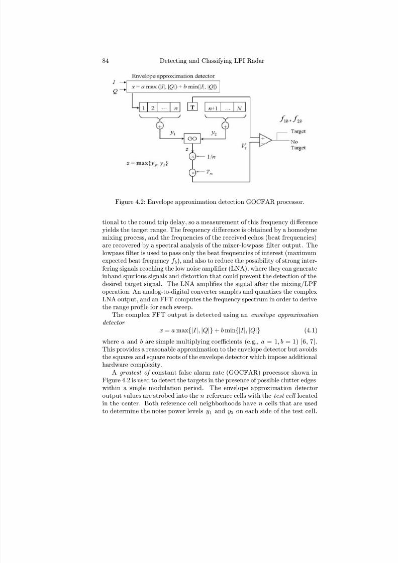
7/17/2019 1596932341 Intercept Radar.pdf
http://slidepdf.com/reader/full/1596932341-intercept-radarpdf 115/891
84 Detecting and Classifying LPI Radar
Figure 4.2: Envelope approximation detection GOCFAR processor.
tional to the round trip delay, so a measurement of this frequency diff erenceyields the target range. The frequency diff erence is obtained by a homodynemixing process, and the frequencies of the received echos (beat frequencies)are recovered by a spectral analysis of the mixer-lowpass filter output. Thelowpass filter is used to pass only the beat frequencies of interest (maximumexpected beat frequency f b), and also to reduce the possibility of strong inter-fering signals reaching the low noise amplifier (LNA), where they can generateinband spurious signals and distortion that could prevent the detection of thedesired target signal. The LNA amplifies the signal after the mixing/LPFoperation. An analog-to-digital converter samples and quantizes the complexLNA output, and an FFT computes the frequency spectrum in order to derivethe range profile for each sweep.
The complex FFT output is detected using an envelope approximation
detector
x = a max|I |, |Q| + b min|I |, |Q| (4.1)
where a and b are simple multiplying coefficients (e.g., a = 1, b = 1) [6, 7].This provides a reasonable approximation to the envelope detector but avoidsthe squares and square roots of the envelope detector which impose additionalhardware complexity.
A greatest of constant false alarm rate (GOCFAR) processor shown inFigure 4.2 is used to detect the targets in the presence of possible clutter edgeswithin a single modulation period. The envelope approximation detector
output values are strobed into the n reference cells with the test cell locatedin the center. Both reference cell neighborhoods have n cells that are usedto determine the noise power levels y1 and y2 on each side of the test cell.

7/17/2019 1596932341 Intercept Radar.pdf
http://slidepdf.com/reader/full/1596932341-intercept-radarpdf 116/891
FMCW Radar 85
Figure 4.3: State transition diagram of the Markov chain used for postdetec-tion integration.
Note that the width of each reference cell or filter is ∆f Hz. The thresholdvoltage V t is obtained by choosing the greatest of y1 and y2, normalizing bythe number of reference cells n and multiplying by the threshold multiplierT . Targets are declared in range for both up slope and down slope (beatfrequencies f 1b, f 2b), when the amplitude of the test filter is greater than thethreshold voltage. Other CFAR architectures can be used, depending on theoperating environment.
For each modulation period, a single target can result in a number of GOCFAR range detections, depending on the target’s extent and the sizeof the range resolution ∆R. Each detection is tagged by its range RT andits azimuth angle θa. To reduce the chance of declaring a false target, post-
detection integration can be used within a single scan. A simple method of performing postdetection integration for each range detection is through theuse of a discrete time Markov chain [8] with N M states followed by a singlescan angle threshold processor. A state transition diagram of a postdetectionintegration Markov chain is shown in Figure 4.3. When the state reachesN X , Θstart = θa, and this marks the beginning of the target position in az-imuth. For each detection at RT , the state of the chain advances one level(with probability of detection p). Upon receiving subsequent reports for thisrange bin from the GOCFAR, the state either moves up or down. For eachsubsequent miss at RT , the state drops one level (with probability q = 1 − p).When the state drops below N Y , Θstop = θa and this marks the end of the

7/17/2019 1596932341 Intercept Radar.pdf
http://slidepdf.com/reader/full/1596932341-intercept-radarpdf 117/891
86 Detecting and Classifying LPI Radar
target’s extent in azimuth.Each postdetection integration output has both the target’s range RT , and
its extent in azimuth ∆Θ = |Θstart − Θstop|. The single scan angle threshold
processor then compares ∆Θ and declares a target at this range and scanif T A ≤ ∆Θ ≤ T B . The thresholds T A (lower limit) and T B (upper limit)depend on the signal-to-noise ratio and are a function of the target’s range,RCS, and any frequency domain STC that is applied. The targets declared oneach scan are normally entered into a track file after going through a gatingprocess followed by a scan-to-scan correlation.
4.3 Transmitted Waveform Design
There are two main challenges in designing a high dynamic range FMCWradar for the detection of small targets against a high density clutter back-ground. The first is generating a frequency sweep that is linear. The second
challenge is controlling the leakage of transmitter phase noise into the receiver.We begin by examining a triangular FMCW waveform and the Doppler
shifted received signal as shown in Figure 4.4. The triangular modulationconsists of two linear frequency modulation sections with positive and nega-tive slopes. With a triangular waveform, the range and Doppler frequency of the detected target can be extracted unambiguously by taking, respectively,the sum and the diff erence of the two beat frequencies. In this section, thetriangular waveform is described, and ways of generating the LPI waveformare discussed.
4.3.1 Triangular Waveform
The frequency of the transmitted waveform for the first section is [9, 10]
f 1(t) = f c − ∆F
2 +
∆F
tmt (4.2)
for 0 < t < tm and zero elsewhere. Here f c is the RF carrier, ∆F is the trans-mit modulation bandwidth, and tm is the modulation period. The modulation(sweep) bandwidth ∆F is chosen to provide the required range resolution
∆R = c
2∆F m (4.3)
Note that the larger the bandwidth, the smaller the resolution and the moreLPI the signal becomes. The rate of frequency change or chirp rate F is
F = ∆F tm
(4.4)

7/17/2019 1596932341 Intercept Radar.pdf
http://slidepdf.com/reader/full/1596932341-intercept-radarpdf 118/891
FMCW Radar 87
Figure 4.4: Linear frequency modulated triangular waveform and the Dopplershifted received signal.
The phase of the transmitted RF signal is
φ1(t) = 2π
t0
f 1(x)dx (4.5)
Assuming that φ0 = 0 at t = 0,
φ1(t) = 2π
f c −
∆F
2
t +
∆F
2tmt2
(4.6)
for 0 < t < tm. The transmit signal is given by
s1(t) = a0 sin 2π
f c −
∆F
2
t +
∆F
2tmt2
(4.7)
The frequency of the transmitted waveform for the second section is similarly
f 2(t) = f c + ∆F
2 −
∆F
tmt (4.8)

7/17/2019 1596932341 Intercept Radar.pdf
http://slidepdf.com/reader/full/1596932341-intercept-radarpdf 119/891
88 Detecting and Classifying LPI Radar
Figure 4.5: A block diagram of an FMCW emitter simulation.
for 0 < t < tm. Finally, the transmit baseband signal is given by
s2(t) = a0 sin 2π
f c +
∆F
2
t −
∆F
2tmt2
(4.9)
Figure 4.5 shows a block diagram of an FMCW emitter simulation. The
sinusoidal carrier is 9.3 GHz and the modulation bandwidth ∆F = 1 GHz.Also shown is the triangular waveform with modulation period tm = 0.5 ×10⁻⁶ s. The power spectral density for the f c = 9.3-GHz FMCW signal with∆F = 1.0 GHz is shown in Figure 4.6 with an SNR = 0 dB. The SNR isdefined in terms of the signal and noise power as
SNR = A2
2σ2 (4.10)
where A is the amplitude of the signal and σ2 is the white Gaussian noisepower. Note the simulation shows that the power spectrum of the linearFMCW waveform is nearly rectangular over the band f c − ∆F/2 < f <f c + ∆F/2 adding to the LPI properties of the transmitted signal.

7/17/2019 1596932341 Intercept Radar.pdf
http://slidepdf.com/reader/full/1596932341-intercept-radarpdf 120/891
FMCW Radar 89
Figure 4.6: The FMCW signal with f c = 9.3 GHz, ∆F = 1.0 GHz, andSNR = 0 dB.
4.3.2 Waveform Spectrum
Without loss of generality, the instantaneous frequency for the first section(4.2) in transmitted waveform can be rewritten as
f 1 = ∆F
tmt + f c (4.11)
for |t| ≤ tm/2 where the carrier frequency f c lies at the beginning of the sweepin frequency. The phase of the signal with instantaneous frequency (4.11) canbe calculated as
φ(t) = 2π
t0
f 1(t)dt = π∆F
tmt2 + 2πf ct (4.12)
where the signal has constant amplitude. To compute the spectrum of thewaveform we use the complex form of the transmit signal as [11]
s(t) = ejφ(t) (4.13)
and obtain the Fourier transform as
s(f ) =
∞
−∞
s(t)e−j2πftdt (4.14)
Substituting in (4.13) and letting α = π∆F/tm
and β = π(f c
− f )
s(f ) =
∞
−∞
ej(αt2+2βt)dt (4.15)

7/17/2019 1596932341 Intercept Radar.pdf
http://slidepdf.com/reader/full/1596932341-intercept-radarpdf 121/891
90 Detecting and Classifying LPI Radar
Using the integral relationships
cos(αt2 + 2β t)dt = π2α
cosβ 2
αC (x) + sinβ 2
αS (x) (4.16)
and sin(αt2 + 2β t)dt =
π
2α
cos
β 2
α
S (x) − sin
β 2
α
C (x)
(4.17)
where
x =
2
πα(αt + β ) (4.18)
and C (x) and S (x) are the Fresnel integrals
C (x) =
x0
cos
πt2
2
dt (4.19)
S (x) = x0
sinπt
2
2
dt (4.20)
the spectrum of a single sweep is then
s(f ) =
π
2αe−jβ
2/α[C (x) + jS (x)]|x(tm/2)−x(tm/2)
(4.21)
and the magnitude squared spectrum is
|s(f )|2 = tm2∆F
[C (x2) − C (x1)]2 + [S (x2) − S (x1)]2 (4.22)
Using (4.22), the spectrum sidelobe roll-off rate may be approximated inthe side lobe region using the Fresnel integral approximations for large x > 5as [11]
C (x) ≈ 1
2 + 1
πx sinπx2
2
− 1
π2x3 cosπx2
2
(4.23)
and
S (x) ≈ 1
2 −
1
πx cos
πx2
2
−
1
π2x3 sin
πx2
2
(4.24)
This shows that the dominant frequency relationship is an inverse x2 termsince x ∝ f through β , and thus the roll-off rate
s(f ) = 10 log10
f 2
(10f )2
= −20dB per decade (4.25)
This spectral behavior is important when considering the out-of-band emis-sions that can degrade the LPI nature of the waveform. Various techniquescan be employed for reducing out-of-band emissions of FMCW waveforms.
These include amplitude tapering on a sweep-by-sweep basis (sometimes re-ferred to as curbing) and using a smooth and finite flyback at the end of eachsweep.

7/17/2019 1596932341 Intercept Radar.pdf
http://slidepdf.com/reader/full/1596932341-intercept-radarpdf 122/891
FMCW Radar 91
4.3.3 Generating Linear FM Waveforms
Linear FM waveforms may be generated by either analog or digital methods.
One method consists of using a voltage controlled oscillator (VCO) to producean approximately linear FM sweep, with the nonlinearities being compensatedin the control voltage ramp [4]. The problem with this approach is being ableto achieve adequate linearity over a wide bandwidth. The oscillators canalso drift with temperature. Another commonly used technique involves adispersive delay line using surface acoustic wave (SAW) technology, but thishas limitations with large time-bandwidth product waveforms tm∆F .
Another approach is to synthesize the sweep in frequency directly by dig-ital means [12]. Advantages of the direct digital synthesizer (DDS) methodinclude: Only the waveform bandwidth (not the time-bandwidth product) islimited by the technology (and circuit complexity), and digital circuits areless likely to be susceptible to temperature drift. Modern DDSs are fully inte-grated, low-cost, single chip solutions that only need an external clock source
for generating the sinusoidal output signals. The DDS benefits from the to-tally digital generation of the output signal, which allows full control of thesignal’s frequency and phase, both with very high precision and resolution.
The sequence of waveform samples can be precomputed , stored, and clockedout of memory. The waveform can be generated at IF or baseband. If gen-erated at IF, a high clock rate is required (that depends on the bandwidth).The preferred approach is generating the complex (I and Q) waveform atbaseband and using a single sideband modulator to put the waveform on acarrier for transmission. The clock rate for this approach is equal to the chirpbandwidth (rather than twice the chirp bandwidth as in the IF approach).
From Figure 4.4, note that the frequency of the waveform increases linearlywith time. The phase for the upsweep is given by (4.6). To synthesize thewaveform in discrete steps, t is replaced by the sample index i and F = ∆F/tmbecomes the angular frequency increment per sample F [12]. The sampledfrequency for the first section for N samples is then
f 1
N, F
= f c −
∆F
2 +
N i=0
F (4.26)
The corresponding phase is then
φ1
N, F
= 2π
N i=0
f 1
N, F
= 2πN i=0
f c − ∆F
2 + F N (4.27)
orφ1 N, F = F N 2 + φ1(0) (4.28)
From these phases, the complex baseband amplitudes can be generated withtwo accumulators as shown in Figure 4.7. The first (frequency) accumulator

7/17/2019 1596932341 Intercept Radar.pdf
http://slidepdf.com/reader/full/1596932341-intercept-radarpdf 123/891
92 Detecting and Classifying LPI Radar
Figure 4.7: Generation of linear FMCW waveform using two accumulators.
is preloaded with the starting frequency f c − ∆F/2. The second (phase)accumulator is loaded with zero. In each clock cycle, the frequency incrementis added to the frequency accumulator and the new frequency is added to thephase accumulator [see (4.26) and (4.27)]. The width of the data path in theaccumulators is given by [12]
n = log2
tmf clk∆F
δ F
(4.29)
where δ F is the bandwidth increment and f clk is the clock frequency.The phase accumulator output (e.g., 2’s complement) is then used to ad-
dress both a sine look-up table (LUT) and a cosine LUT. Only one cycle of the sine and cosine waveform needs to be stored in the LUT, since the wave-form repeats every 2π. The output LUT resolution depends on the fidelityof the signal required, and the bandwidth and resolution of the digital-to-analog converter (DAC) that is available. The lowpass filter (LPF) is neededto reject the repeated spectra around the clock frequency and multiples of the clock frequency [13]. If not eliminated, the high frequency componentscause spurious signals out of the single-sideband modulator (SSBM) used forupconversion on to the RF carrier f c. The SSBM uses the DDS as a referencefor a phase-locked-loop stabilized VCO, where the DDS is driven by a high
speed reference clock.
2
2Software-driven digital upconversions are also an area of development that is promisingfor FMCW generation. They can currently provide an intermediate stage upconversion,

7/17/2019 1596932341 Intercept Radar.pdf
http://slidepdf.com/reader/full/1596932341-intercept-radarpdf 124/891
FMCW Radar 93
Figure 4.8: Staircase approximation of the phase φ(t).
The SSBM mixes the video modulating signal f m with the carrier f c andsuppresses either f c + f m or f c − f m. How well the sideband is suppressedcan be quantified as a function of |I |, |Q|, and the phase error from perfectquadrature ∆φ as
s = 10 log10
1 +
|I |2
|Q|2 − 2
|I |2
|Q|2 cos ∆φ
(4.30)
A detailed noise analysis of the approach above was completed by [14].The analysis investigates a staircase phase approximation of the FMCWchirp, and examines the spectrum of the transmitted and received signal.The noise caused by the quantization error is then analyzed. It shows thatthe FMCW signal can be digitally generated using a staircase approximationof its quadratic phase term, without requiring a filter to smooth the signalon transmission or reception. The noise on the transmitted waveform is notusually a problem, except that demodulation of the return signal uses thistransmitted waveform as a reference.
A digital approximation of the parabolic phase is shown in Figure 4.8, andensures that each step of the phase staircase is a rectangular function. Alsoshown is the holding time or subpulse width. The amplitude and phase noiseproduce a noise power spectral density on the transmitted signal that dependson the subpulse width T and the number of bits of the uniform quantizer n.The requirement for good spectral conditions is [14]
T < 1
5Ba(4.31)
where Ba is the bandwidth after demodulation (on the order of 100 Hz). If the amplitude and phase noise errors are both uniformly distributed over the
relaxing the requirements on the DAC and LUT resolution.

7/17/2019 1596932341 Intercept Radar.pdf
http://slidepdf.com/reader/full/1596932341-intercept-radarpdf 125/891
94 Detecting and Classifying LPI Radar
bandwidth of 1/T , and the spectral contributions of individual subpulses eachcontain a constant error, the power spectral density (PSD) is
PSD = T
12 × 22nsinc2
ωT
2
V2
Hz (4.32)
Example 1: Determine the number of bits required in the accumulatordata path if the modulation period tm = 5.0 μs, ∆F = 500 MHz, the clockfrequency f clk = 500 MHz, and the bandwidth increment δ F = 1 MHz.Using (4.29)
n = log2
1.25(106)
= 20 bits (4.33)
Example 2: Consider a subpulse period T = 8 μs and a 12-bit quantizer.(a) Determine the bandwidth over which the total noise power will be spread.(b) Determine the noise level due to amplitude and phase noise errors.
For (a), 1/T = 1/8μs = 125 kHz. Note that this is much larger than thelow frequency stages of the radar receiver (e.g., 100 Hz). For (b), from (4.32)above,
PSD = 10 log
8 μs
12 × 224
= 134 dB
V2
Hz (4.34)
below the received carrier, which is quite good.Recently a DDS was reported using InP double heterojunction bipolar
transistor technology. With a single 12-bit phase accumulator and a readonly memory LUT phase converter, the DDS is capable of synthesizing outputfrequencies up to 12 GHz in steps that are 1/4,096 of the 24 GHz clock rate[15]. The measured spurious free dynamic range (SFDR) is 30.7 dB and theaverage SFDR over all frequency control words is 40.4 dB. The significance
of this is that the radar signals can be generated directly in the desired RFband.
In summary, the DDS is a more complex approach to generating theFMCW waveform than using a VCO. It has the advantage however, thatit provides a perfectly linear sweep and has greater stability which is espe-cially important in LPI emitters where sweep-to-sweep Doppler processing isrequired.
4.4 Receiver-Transmitter Isolation
One of the greatest problems facing CW radar designers is detecting targetreturns on the order of a picowatt or less in the presence of a few watts of
transmitted power. This is due to the problem of achieving sufficient isolationbetween transmitter and receiver, since the transmission and reception aresimultaneous. The main two problems are:
7/17/2019 1596932341 Intercept Radar.pdf
http://slidepdf.com/reader/full/1596932341-intercept-radarpdf 126/891
FMCW Radar 95
• Transmitter noise sidebands can hide valid targets.
• Power leakage desensitizes the receiver.
Although a dual antenna configuration that is well isolated is a possiblesolution, numerous applications require only a single antenna (e.g., a missileseeker). In this section, a review of transmission line basics is presented,followed by a discussion of two single antenna systems; one using a circulator,and one using an RPC.
4.4.1 Transmission Line Basics
In the analysis of transmission line performance [16], the voltage re fl ection
coe ffi cient , Γ of a transmission line-antenna interface is defined as
Γ = reflected voltage
incident voltage
(4.35)
and is generally a complex quantity
Γ = |Γ|ejθl (4.36)
where |Γ| is the magnitude, and never greater than unity (|Γ| ≤ 1). The phaseθl is the angle between the incident and reflected voltages at the receivingend, and is usually called the phase angle of the reflection coefficient.
The general solutions of the transmission line equations consist of twowaves traveling in opposite directions with unequal amplitudes. These wavesare called standing waves . The ratio of the maximum voltage of the standingwave pattern to the minimum voltage is defined as the voltage standing wave
ratio ρV
ρV = |V Max ||V Min |
(4.37)
and is usually found using Smith charts. The standing wave ratio results fromthe fact that the two traveling wave components add in phase at some points,and subtract it at other points. The standing wave ratio ρV is related to thereflection coefficient by
ρV = 1 + |Γ|
1 − |Γ| (4.38)
and solving for |Γ|,
|Γ| = ρV − 1
ρV + 1 (4.39)
These results can be used to quantify the various antenna configurations forFMCW emitters.
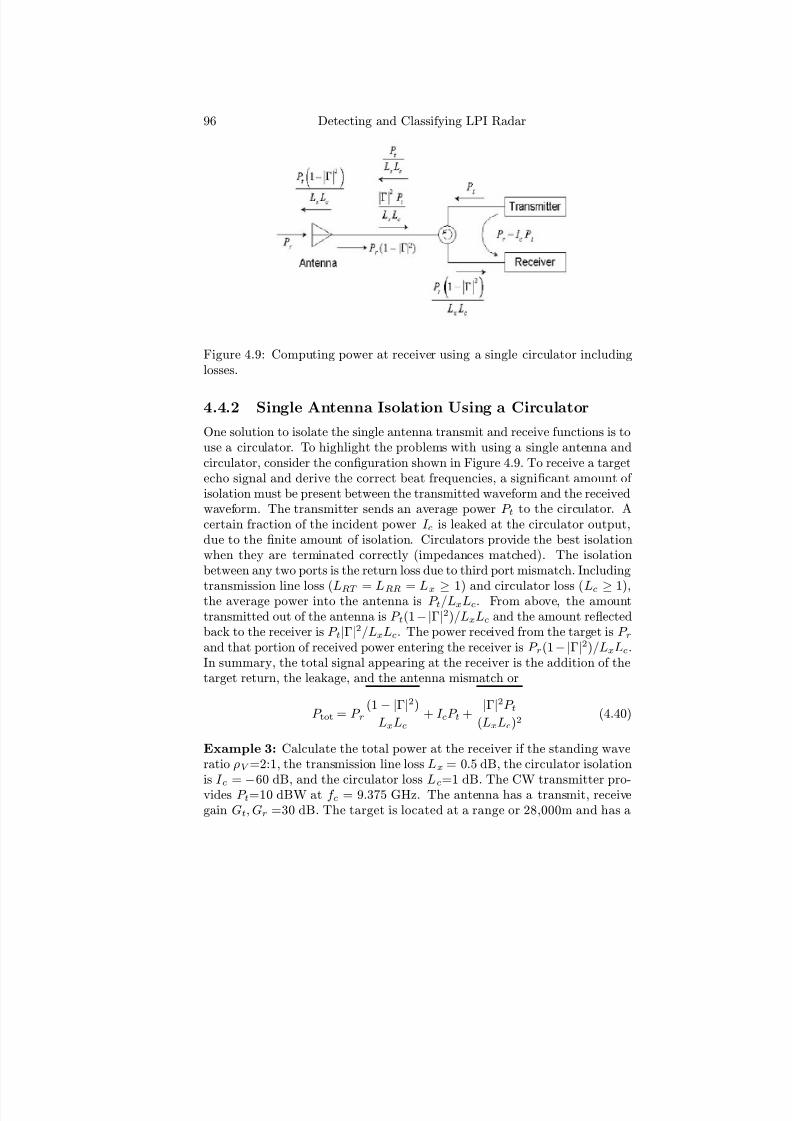
7/17/2019 1596932341 Intercept Radar.pdf
http://slidepdf.com/reader/full/1596932341-intercept-radarpdf 127/891
96 Detecting and Classifying LPI Radar
Figure 4.9: Computing power at receiver using a single circulator includinglosses.
4.4.2 Single Antenna Isolation Using a Circulator
One solution to isolate the single antenna transmit and receive functions is touse a circulator. To highlight the problems with using a single antenna andcirculator, consider the configuration shown in Figure 4.9. To receive a targetecho signal and derive the correct beat frequencies, a significant amount of isolation must be present between the transmitted waveform and the receivedwaveform. The transmitter sends an average power P t to the circulator. Acertain fraction of the incident power I c is leaked at the circulator output,due to the finite amount of isolation. Circulators provide the best isolationwhen they are terminated correctly (impedances matched). The isolationbetween any two ports is the return loss due to third port mismatch. Including
transmission line loss (LRT = LRR = Lx ≥ 1) and circulator loss (Lc ≥ 1),the average power into the antenna is P t/LxLc. From above, the amounttransmitted out of the antenna is P t(1 − |Γ|2)/LxLc and the amount reflectedback to the receiver is P t|Γ|
2/LxLc. The power received from the target is P rand that portion of received power entering the receiver is P r(1 − |Γ|2)/LxLc.In summary, the total signal appearing at the receiver is the addition of thetarget return, the leakage, and the antenna mismatch or
P tot = P r(1 − |Γ|2)
LxLc+ I cP t +
|Γ|2P t(LxLc)2
(4.40)
Example 3: Calculate the total power at the receiver if the standing waveratio ρV =2:1, the transmission line loss Lx = 0.5 dB, the circulator isolation
is I c = −60 dB, and the circulator loss Lc=1 dB. The CW transmitter pro-vides P t=10 dBW at f c = 9.375 GHz. The antenna has a transmit, receivegain Gt, Gr =30 dB. The target is located at a range or 28,000m and has a
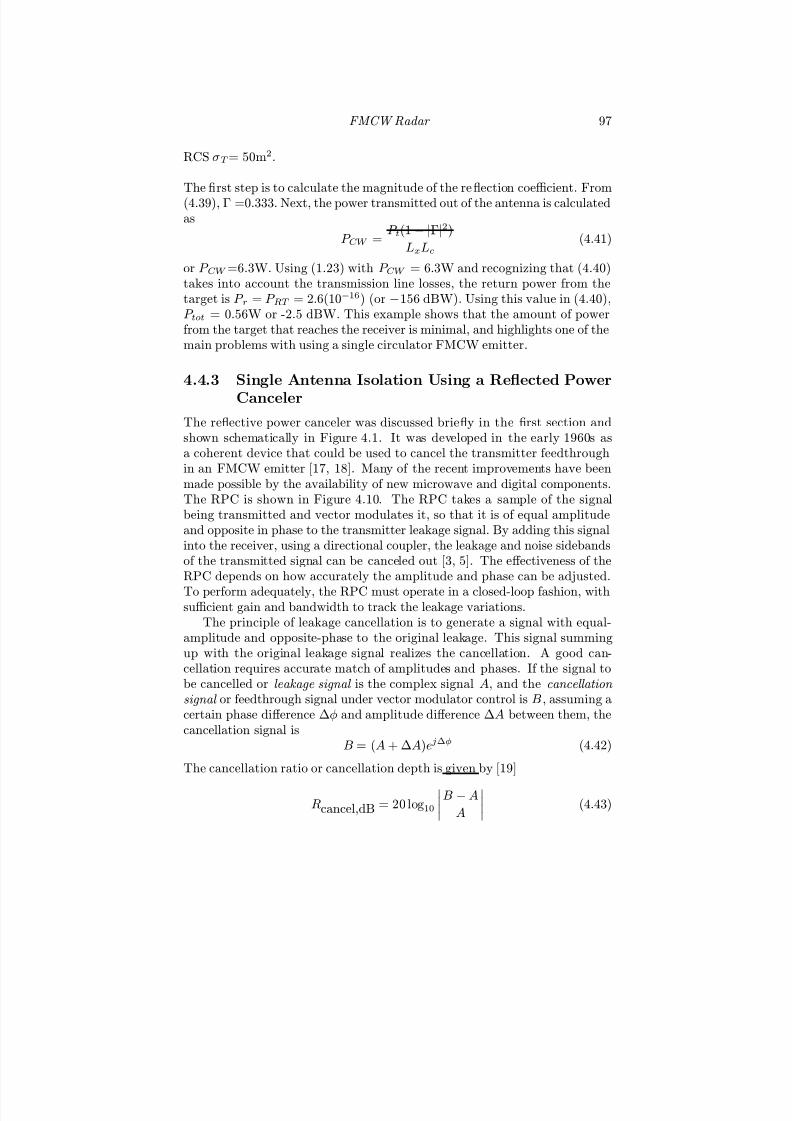
7/17/2019 1596932341 Intercept Radar.pdf
http://slidepdf.com/reader/full/1596932341-intercept-radarpdf 128/891
FMCW Radar 97
RCS σT = 50m2.
The first step is to calculate the magnitude of the reflection coefficient. From(4.39), Γ =0.333. Next, the power transmitted out of the antenna is calculatedas
P CW = P t(1 − |Γ|2)
LxLc(4.41)
or P CW =6.3W. Using (1.23) with P CW = 6.3W and recognizing that (4.40)takes into account the transmission line losses, the return power from thetarget is P r = P RT = 2.6(10−16) (or −156 dBW). Using this value in (4.40),P tot = 0.56W or -2.5 dBW. This example shows that the amount of powerfrom the target that reaches the receiver is minimal, and highlights one of themain problems with using a single circulator FMCW emitter.
4.4.3 Single Antenna Isolation Using a Reflected Power
Canceler
The reflective power canceler was discussed briefly in the first section andshown schematically in Figure 4.1. It was developed in the early 1960s asa coherent device that could be used to cancel the transmitter feedthroughin an FMCW emitter [17, 18]. Many of the recent improvements have beenmade possible by the availability of new microwave and digital components.The RPC is shown in Figure 4.10. The RPC takes a sample of the signalbeing transmitted and vector modulates it, so that it is of equal amplitudeand opposite in phase to the transmitter leakage signal. By adding this signalinto the receiver, using a directional coupler, the leakage and noise sidebandsof the transmitted signal can be canceled out [3, 5]. The eff ectiveness of theRPC depends on how accurately the amplitude and phase can be adjusted.
To perform adequately, the RPC must operate in a closed-loop fashion, withsufficient gain and bandwidth to track the leakage variations.
The principle of leakage cancellation is to generate a signal with equal-amplitude and opposite-phase to the original leakage. This signal summingup with the original leakage signal realizes the cancellation. A good can-cellation requires accurate match of amplitudes and phases. If the signal tobe cancelled or leakage signal is the complex signal A, and the cancellation
signal or feedthrough signal under vector modulator control is B , assuming acertain phase diff erence ∆φ and amplitude diff erence ∆A between them, thecancellation signal is
B = (A + ∆A)ej∆φ (4.42)
The cancellation ratio or cancellation depth is given by [19]
Rcancel,dB = 20 log10
B − A
A
(4.43)
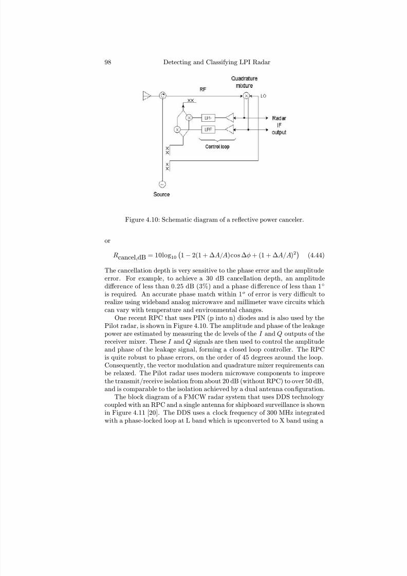
7/17/2019 1596932341 Intercept Radar.pdf
http://slidepdf.com/reader/full/1596932341-intercept-radarpdf 129/891
98 Detecting and Classifying LPI Radar
Figure 4.10: Schematic diagram of a reflective power canceler.
or
Rcancel,dB = 10log10
1 − 2(1 + ∆A/A)cos∆φ + (1 + ∆A/A)2
(4.44)
The cancellation depth is very sensitive to the phase error and the amplitudeerror. For example, to achieve a 30 dB cancellation depth, an amplitudediff erence of less than 0.25 dB (3%) and a phase diff erence of less than 1
is required. An accurate phase match within 1o of error is very difficult to
realize using wideband analog microwave and millimeter wave circuits whichcan vary with temperature and environmental changes.
One recent RPC that uses PIN (p into n) diodes and is also used by thePilot radar, is shown in Figure 4.10. The amplitude and phase of the leakagepower are estimated by measuring the dc levels of the I and Q outputs of thereceiver mixer. These I and Q signals are then used to control the amplitudeand phase of the leakage signal, forming a closed loop controller. The RPCis quite robust to phase errors, on the order of 45 degrees around the loop.Consequently, the vector modulation and quadrature mixer requirements canbe relaxed. The Pilot radar uses modern microwave components to improvethe transmit/receive isolation from about 20 dB (without RPC) to over 50 dB,and is comparable to the isolation achieved by a dual antenna configuration.
The block diagram of a FMCW radar system that uses DDS technology
coupled with an RPC and a single antenna for shipboard surveillance is shownin Figure 4.11 [20]. The DDS uses a clock frequency of 300 MHz integratedwith a phase-locked loop at L band which is upconverted to X band using a
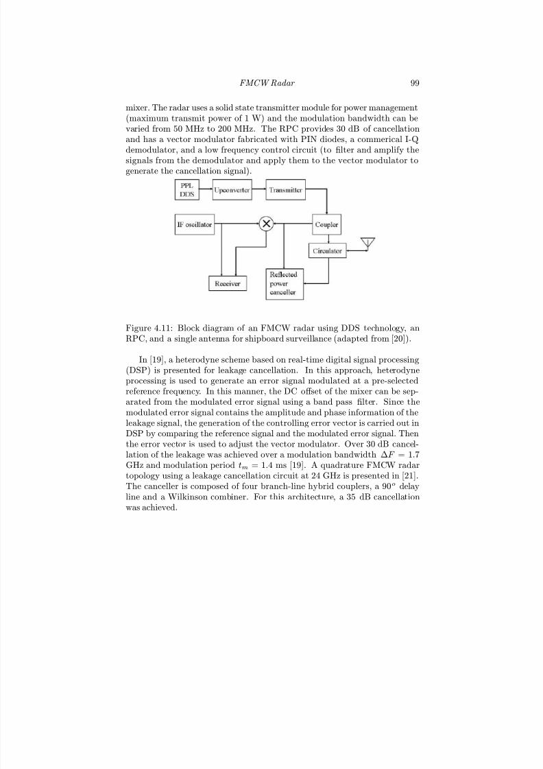
7/17/2019 1596932341 Intercept Radar.pdf
http://slidepdf.com/reader/full/1596932341-intercept-radarpdf 130/891
FMCW Radar 99
mixer. The radar uses a solid state transmitter module for power management(maximum transmit power of 1 W) and the modulation bandwidth can bevaried from 50 MHz to 200 MHz. The RPC provides 30 dB of cancellationand has a vector modulator fabricated with PIN diodes, a commerical I-Qdemodulator, and a low frequency control circuit (to filter and amplify thesignals from the demodulator and apply them to the vector modulator togenerate the cancellation signal).
Figure 4.11: Block diagram of an FMCW radar using DDS technology, anRPC, and a single antenna for shipboard surveillance (adapted from [20]).
In [19], a heterodyne scheme based on real-time digital signal processing(DSP) is presented for leakage cancellation. In this approach, heterodyneprocessing is used to generate an error signal modulated at a pre-selectedreference frequency. In this manner, the DC off set of the mixer can be sep-
arated from the modulated error signal using a band pass filter. Since themodulated error signal contains the amplitude and phase information of theleakage signal, the generation of the controlling error vector is carried out inDSP by comparing the reference signal and the modulated error signal. Thenthe error vector is used to adjust the vector modulator. Over 30 dB cancel-lation of the leakage was achieved over a modulation bandwidth ∆F = 1.7GHz and modulation period tm = 1.4 ms [19]. A quadrature FMCW radartopology using a leakage cancellation circuit at 24 GHz is presented in [21].The canceller is composed of four branch-line hybrid couplers, a 90o delayline and a Wilkinson combiner. For this architecture, a 35 dB cancellationwas achieved.
7/17/2019 1596932341 Intercept Radar.pdf
http://slidepdf.com/reader/full/1596932341-intercept-radarpdf 131/891
100 Detecting and Classifying LPI Radar
4.5 The Received Signal
The received signal from a stationary target is the transmit signal delayed in
time by the round-trip propagation time (or transit time) to the target andback (td), with reduced amplitude b0 [3]
sr(t) = b0a0
s1(t − td) (4.45)
or
s1r(t) = b0 sin 2π
f c −
∆F
2
(t − td) +
∆F
2tm(t − td)2
(4.46)
For the homodyne FMCW emitter, the receive signal is mixed with the trans-mit signal. The beat frequencies are derived as the diff erence between thetransmitted and received signals. The beat frequency is sometimes referredto as an intermediate frequency, although the information is not modulated
onto a conventional carrier [9]. The mixer output beat frequency signal is
s1b(t) = c0 cos 2π
f c −
∆F
2
td −
∆F
2tmt2d +
∆F
tmtdt
(4.47)
For the second segment of the triangular waveform, the mixer output beatfrequency signal is
s2b(t) = c0 cos 2π
f c +
∆F
2
td +
∆F
2tmt2d −
∆F
tmtdt
(4.48)
Equations (4.47) and (4.48) contain a frequency term that is time varyingand phase terms that are not. The beat frequency is the third term in (4.47)and (4.48)
f b = ∆F
tmtd =
2R∆F
ctm=
2R
cF (4.49)
where the delay time td = 2R/c for a stationary target at a range of R. If thetarget is moving with velocity V , the beat frequency for the first segment is
f 1b = 2R∆F
ctm−
2V
λ =
2R
cF −
2V
λ (4.50)
and the beat frequency for the second segment is
f 2b = 2R∆F
ctm+
2V
λ =
2R
cF +
2V
λ (4.51)
where the second term is due to the target’s Doppler frequency. For multipletargets, multiple beat frequencies would be present and would depend on eachtarget’s range and velocity.

7/17/2019 1596932341 Intercept Radar.pdf
http://slidepdf.com/reader/full/1596932341-intercept-radarpdf 132/891
FMCW Radar 101
Figure 4.12: ASCM LPI emitter-ship scenario.
In summary, the advantages of the linear FMCW waveform include:(a) the presence of LPI operation with an efficient utilization of the spec-trum, (b) the waveform is easier to implement than phase-coded modulationif there are no strict demands on linearity over a wide bandwidth, and (c)the received signal can be processed using one multiplication with a matchedreference signal, with the range being resolved using spectral analysis.
4.6 LPI Search Mode Processing
To illustrate LPI search mode processing, consider an antiship cruise missilewith a seeker (f c = 9.375 GHz) flying inbound to a target ship with RCS =σT . The incremental backscattering coefficient of the sea surface is σo. TheLPI seeker comes on at a range of R = 28,000m (15 nmi) from the ship.Figure 4.12 shows the missile-ship scenario being investigated. The emitteris flown at 300 m/s (Mach 1) at an altitude of h = 70m toward the ship fora period of 91s. Note that this scenario assumes initially that the ship is notmoving. The scenario is analogous to the LPI radar being stationary andthe target approaching at 300m/s. In the search mode, the emitter uses, forexample, the conventional scan shown in Figure 1.4(a) and makes a singlescan every 3s with a scan rate of 70 deg/s. At end game (700m from target),the missile dives to the ship for impact.
The first step in designing the LPI seeker is to determine the modulationbandwidth ∆F (peak-to-peak frequency deviation) in order to give the re-quired range resolution. For example, the ASCM might require a ∆R = 0.3m
7/17/2019 1596932341 Intercept Radar.pdf
http://slidepdf.com/reader/full/1596932341-intercept-radarpdf 133/891
102 Detecting and Classifying LPI Radar
range resolution, in order to calculate the ship orientation and select a wa-terline aimpoint with good accuracy. With this range resolution, the shipreturns could easily extend over a large number of range bins, depending onthe aspect angle. Recall that the ideal range resolution is
∆R = c
2∆F m (4.52)
For ∆R = 0.3m, a ∆F = 500 MHz is chosen. To increase the signal toclutter ratio, a ∆R equivalent to the size of the ship may be selected so thatthe entire ship’s return lies within a single range bin. This approach wouldrequire a smaller ∆F .
The modulation period is chosen next, and two factors must be considered.The first consideration is that
tm < ∆R
V t(4.53)
where V t is the maximum closing velocity of the target. This relationshiprequires that the target must remain in a range bin for at least an entiremodulation period tm. Otherwise, the target return will smear across severalrange bins. The second consideration is that tm should be several timesthe maximum round-trip delay td, of the target’s return signal. This is inorder to minimize the loss in eff ective transmit bandwidth and power andto also provide a high velocity resolution [9]. Since an acquisition range of R = 28, 000m corresponds to a maximum round-trip delay td = 186.7 μs, amodulation period of tm = 1 ms is chosen (≈ 5.5td).
The resulting coherent processing interval is
t0 = tm − td (4.54)
The spectral width of the beat frequency is the inverse of the coherent process-ing interval or
∆w = 1
t0=
1
tm − td≈
1
tm(4.55)
and is the Doppler shift that causes a range error of exactly one range bin.The eff ect that a Doppler shift can change the apparent range of the target isthe well-known FMCW range-Doppler cross-coupling e ff ect . That is, the un-ambiguous Doppler frequency is f u = ±1/2t0 Hz. The corresponding velocityresolution or fi rst blind speed is
∆v = λ∆w
2 m/s (4.56)
The first blind speed is the speed at which the Doppler goes through onecomplete cycle from one sweep to the next (beat frequency increases byone cycle per sweep) [3]. For our example, with a target acquisition range

7/17/2019 1596932341 Intercept Radar.pdf
http://slidepdf.com/reader/full/1596932341-intercept-radarpdf 134/891
FMCW Radar 103
R = 28 km and a td = 186.7 μs, the coherent processing interval t0 = 0.81ms and the spectral width ∆w = 1.23 kHz. The resulting first blind speed is∆v = 19.7m/s.
For the first section of the triangular waveform, the partial overlap resultsin a reduced processed bandwidth. The eff ective bandwidth is
∆F = ∆F
1 −
tdtm
Hz (4.57)
with an eff ective time bandwidth product of t0∆F . The range resolution isalso slightly degraded as
∆R = c
2∆F =
c
2∆F (1 − td/tm) m (4.58)
Continuing the example above, with td = 186.7 μs, ∆F = 406.7 MHz, ∆R =0.37m, and the eff ective time-bandwidth product t0∆F = 330.75× 10³. The
large time-bandwidth product contributes to the LPI nature of the radar.The resulting beat frequencies are of the form
f 1b = 2R∆F
ct0−
2V
λ (4.59)
and
f 2b = 2R∆F
ct0+
2V
λ (4.60)
Using the numbers from the example above with V max = 300m/s, the corre-sponding maximum beat frequency is f max
b = 93.35 MHz.The analog-to-digital converter section of the LPI radar receiver must
sample at least twice the highest beat frequency or
f s = 2
2R∆
F
ct0+ 2V
λ
samples/s (4.61)
resulting in the number of samples within a coherent processing interval of N F = f st0. With f max
b = 93.35 MHz, f s = 186.7 MS/s.To resolve the multiple echoes from the clutter and targets, an FFT
process is used for frequency analysis. The signal after frequency analysisis a coherent video signal. Since the FFT requires integer powers of 2, theFFT size is chosen to be N = 2x ≥ N F . To capture this many samples, theADC sampling frequency must be
f s = N
t0samples/s (4.62)
with the sampling frequency and an FFT size of N
, the resulting fi
lter widthis
∆f = f sN
(4.63)
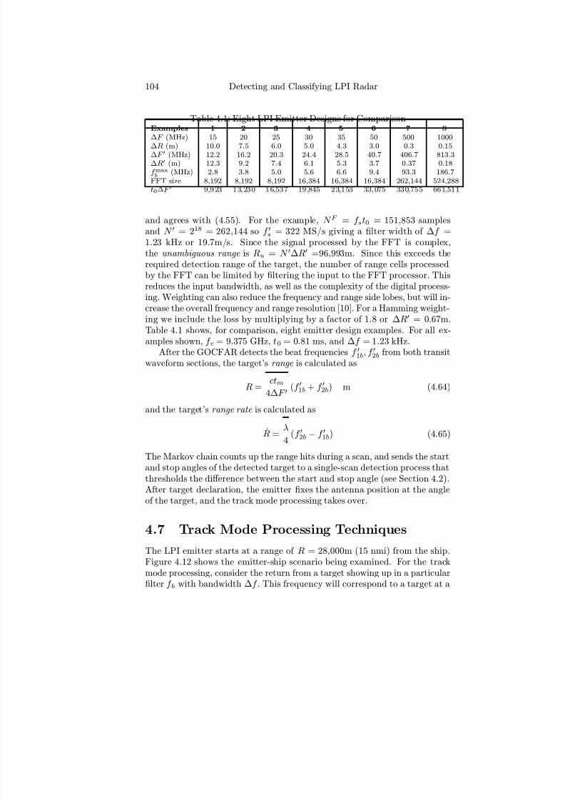
7/17/2019 1596932341 Intercept Radar.pdf
http://slidepdf.com/reader/full/1596932341-intercept-radarpdf 135/891
104 Detecting and Classifying LPI Radar
Table 4.1: Eight LPI Emitter Designs for ComparisonExamples 1 2 3 4 5 6 7 8
∆F (MHz) 15 20 25 30 35 50 500 1000∆R (m) 10.0 7.5 6.0 5.0 4.3 3.0 0.3 0.15∆F (MHz) 12.2 16.2 20.3 24.4 28.5 40.7 406.7 813.3∆R (m) 12.3 9.2 7.4 6.1 5.3 3.7 0.37 0.18f maxb
(MHz) 2.8 3.8 5.0 5.6 6.6 9.4 93.3 186.7FFT size 8,192 8,192 8,192 16,384 16,384 16,384 262,144 524,288t0∆F 9,923 13,230 16,537 19,845 23,153 33,075 330,755 661,511
and agrees with (4.55). For the example, N F = f st0 = 151,853 samplesand N = 218 = 262,144 so f s = 322 MS/s giving a filter width of ∆f =1.23 kHz or 19.7m/s. Since the signal processed by the FFT is complex,the unambiguous range is Ru = N ∆R =96,993m. Since this exceeds therequired detection range of the target, the number of range cells processedby the FFT can be limited by filtering the input to the FFT processor. Thisreduces the input bandwidth, as well as the complexity of the digital process-ing. Weighting can also reduce the frequency and range side lobes, but will in-crease the overall frequency and range resolution [10]. For a Hamming weight-ing we include the loss by multiplying by a factor of 1.8 or ∆R = 0.67m.Table 4.1 shows, for comparison, eight emitter design examples. For all ex-amples shown, f c = 9.375 GHz, t0 = 0.81 ms, and ∆f = 1.23 kHz.
After the GOCFAR detects the beat frequencies f 1b, f 2b from both transitwaveform sections, the target’s range is calculated as
R = ctm4∆F
(f 1b + f 2b) m (4.64)
and the target’s range rate is calculated as
R = λ
4 (f 2b − f 1b) (4.65)
The Markov chain counts up the range hits during a scan, and sends the startand stop angles of the detected target to a single-scan detection process thatthresholds the diff erence between the start and stop angle (see Section 4.2).After target declaration, the emitter fixes the antenna position at the angleof the target, and the track mode processing takes over.
4.7 Track Mode Processing Techniques
The LPI emitter starts at a range of R = 28,000m (15 nmi) from the ship.
Figure 4.12 shows the emitter-ship scenario being examined. For the trackmode processing, consider the return from a target showing up in a particularfilter f b with bandwidth ∆f . This frequency will correspond to a target at a
7/17/2019 1596932341 Intercept Radar.pdf
http://slidepdf.com/reader/full/1596932341-intercept-radarpdf 136/891
FMCW Radar 105
range R where
R = cf bt02∆F
(4.66)
Consequently if the target range is varying, it may be tracked by adjusting thesweep bandwidth ∆F in order to keep the beat frequency equal to f b. Thisrelaxes the LPF requirements at the receiver frontend. Also recall that therange resolution ∆R = c/2∆F . The ratio of these gives the range resolutionexpressed as a fraction of the range
∆R
R =
1
f bt0(4.67)
and is a constant. That is, the emitter will measure the range to the targetwith a resolution that is proportional to the range. As the range-to-targetgets smaller, the bandwidth ∆F gets larger. For example, if the target atR = 28,000 is acquired on the first transmit waveform, the target shows up
at filter number 75,675 or f b = 75, 675 ∗ 1.23 kHz = 93.1 MHz. In order tokeep the target at this beat frequency, the sweep bandwidth is calculated as
∆F = cf bt0
2R =
1.13 × 10¹³
R Hz (4.68)
For an endgame range-to-target of R = 700m, ∆F = 16.2 GHz. Ablock diagram of the track processing is shown in Figure 4.13. Note thatthe major advantage of this technique is that the (narrow) bandpass filteris now centered on f b. Since the range to the moving target is changingwith time, a range tracker (in Doppler space) is required that is constantlyadjusted to keep the target locked in range. After the range is computed, therequired sweep bandwidth is recalculated and sent to the triangular waveform
generator.Another approach to the track processing is to keep the sweep bandwidth
constant, and to allow the target’s beat frequency to change. The target’sposition can be followed in signal processing by monitoring the position of the FFT peak detector output. The advantage of this approach is that thereceiver LPF used in the search mode can also be used for the track processing,at the expense of integrating a larger noise component.
4.8 Eff ect of Sweep Nonlinearities
Frequency sweep nonlinearities (frequency instability in the transmitter) actto broaden the spectral width of the target’s beat frequency. The requirement
on frequency stability in the transmitter is investigated in [10, 22], and tech-niques to correct for these nonlinearities are examined in [23]. To quantifythese eff ects, a nonlinear term can be added to (4.8) as [10]

7/17/2019 1596932341 Intercept Radar.pdf
http://slidepdf.com/reader/full/1596932341-intercept-radarpdf 137/891
106 Detecting and Classifying LPI Radar
Figure 4.13: Block diagram of the track processing, for the triangular homo-dyne FMCW emitter.
f 2n(t) = f c + ∆F
2 −
∆F
tmt + An sin 2πf nt (4.69)
where 0 < t < tm and An is the amplitude of the sinusoidal nonlinearity, andf n is the frequency of the sinusoidal nonlinearity. The transmitted signal is
s2n(t) = a0 sin 2π
f c +
∆F
2
t −
∆F
2tmt2 +
An
2πf n(1 − cos2πf nt)
(4.70)
The corresponding mixer output beat frequency signal can be shown to havethe form
s2bn(t) = c0 cos 2π
f c +
∆F
2
td +
∆F
2tmt2d −
∆F
tmtdt
+ An
2πf n[cos2πf n(t − td) − cos2πf nt]
for 0 < t < tm. From this expression, the eff ects of the nonlinearity can be
evaluated and their significance evaluated.

7/17/2019 1596932341 Intercept Radar.pdf
http://slidepdf.com/reader/full/1596932341-intercept-radarpdf 138/891
FMCW Radar 107
Figure 4.14: Performance of a three-sweep canceler on S-band FMCW radar(i-canceled, ii-uncanceled) [3] ( cIEE 1992).
4.9 Moving Target Indication Filtering
A moving target indication (MTI) filter can also be added to the FMCWsignal processing chain, and operates in a manner similar to a pulsed radar[3]. Figure 4.14 shows the operation of an MTI canceler, an experimental S-band FMCW radar built at Philips Research Laboratories. The upper traceshows the video A-scope picture from one sweep of the radar. The lower traceshows the signal at the output of a digital three-sweep MTI canceler with morethan 40 dB of cancellation. Moving target Doppler (MTD) processing can beimplemented by measuring the rate of change of phase of the output of eachFFT range bin, from one sweep to the next, as shown in Figure 4.15. Thiscapability can be added quite easily to existing FMCW radars.
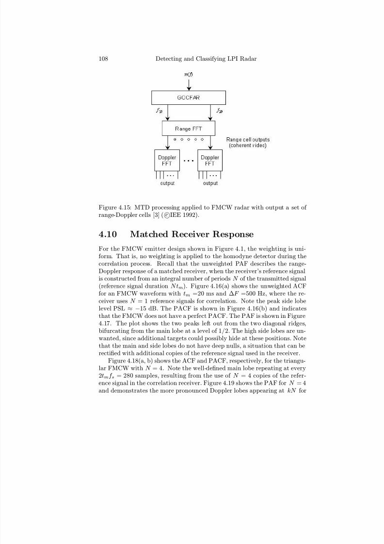
7/17/2019 1596932341 Intercept Radar.pdf
http://slidepdf.com/reader/full/1596932341-intercept-radarpdf 139/891
108 Detecting and Classifying LPI Radar
Figure 4.15: MTD processing applied to FMCW radar with output a set of range-Doppler cells [3] ( cIEE 1992).
4.10 Matched Receiver Response
For the FMCW emitter design shown in Figure 4.1, the weighting is uni-form. That is, no weighting is applied to the homodyne detector during thecorrelation process. Recall that the unweighted PAF describes the range-Doppler response of a matched receiver, when the receiver’s reference signalis constructed from an integral number of periods N of the transmitted signal
(reference signal duration N tm). Figure 4.16(a) shows the unweighted ACFfor an FMCW waveform with tm =20 ms and ∆F =500 Hz, where the re-ceiver uses N = 1 reference signals for correlation. Note the peak side lobelevel PSL ≈ −15 dB. The PACF is shown in Figure 4.16(b) and indicatesthat the FMCW does not have a perfect PACF. The PAF is shown in Figure4.17. The plot shows the two peaks left out from the two diagonal ridges,bifurcating from the main lobe at a level of 1/2. The high side lobes are un-wanted, since additional targets could possibly hide at these positions. Notethat the main and side lobes do not have deep nulls, a situation that can berectified with additional copies of the reference signal used in the receiver.
Figure 4.18(a, b) shows the ACF and PACF, respectively, for the triangu-lar FMCW with N = 4. Note the well-defined main lobe repeating at every2tmf s = 280 samples, resulting from the use of N = 4 copies of the refer-
ence signal in the correlation receiver. Figure 4.19 shows the PAF for N = 4and demonstrates the more pronounced Doppler lobes appearing at kN for

7/17/2019 1596932341 Intercept Radar.pdf
http://slidepdf.com/reader/full/1596932341-intercept-radarpdf 140/891
FMCW Radar 109
Figure 4.16: Triangular FMCW (a) ACF and (b) PACF with ∆F = 500 Hz,tm = 20 ms, and N = 1.
Figure 4.17: Triangular FMCW PAF with ∆F = 500 Hz, tm = 20 ms, andN = 1.
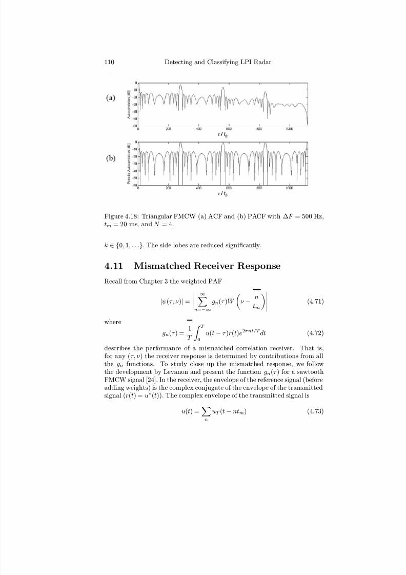
7/17/2019 1596932341 Intercept Radar.pdf
http://slidepdf.com/reader/full/1596932341-intercept-radarpdf 141/891
110 Detecting and Classifying LPI Radar
Figure 4.18: Triangular FMCW (a) ACF and (b) PACF with ∆F = 500 Hz,tm = 20 ms, and N = 4.
k ∈ 0, 1, . . .. The side lobes are reduced significantly.
4.11 Mismatched Receiver Response
Recall from Chapter 3 the weighted PAF
|ψ(τ , ν )| =
∞n=−∞
gn(τ )W ν −
n
tm (4.71)
where
gn(τ ) = 1
T
T 0
u(t − τ )r(t)e2πnt/T dt (4.72)
describes the performance of a mismatched correlation receiver. That is,for any (τ , ν ) the receiver response is determined by contributions from allthe gn functions. To study close up the mismatched response, we followthe development by Levanon and present the function gn(τ ) for a sawtoothFMCW signal [24]. In the receiver, the envelope of the reference signal (beforeadding weights) is the complex conjugate of the envelope of the transmittedsignal (r(t) = u∗(t)). The complex envelope of the transmitted signal is
u(t) =n
uT (t − ntm) (4.73)

7/17/2019 1596932341 Intercept Radar.pdf
http://slidepdf.com/reader/full/1596932341-intercept-radarpdf 142/891
FMCW Radar 111
Figure 4.19: Triangular FMCW PAF with N = 4.
for n = 0, ±1, ±2, · · · , and
uT (t) = exp
jπ∆F
t −
tm2
2
tm(4.74)
where 0 ≤ t ≤ tm and zero elsewhere. Using (4.74) and (4.73) and thereference signal r(t) = u∗(t) in (4.72)
gn(τ ) =
τ
tm
sinα
α + (−1)n
1 −
τ
tm
sin(πn − α)
πn − α
ejπnτ /tm (4.75)
whereα =
πτ
tm[∆F (tm − τ ) + n] (4.76)
and is shown in Figure 4.20(a) for ∆F = 500 Hz and tm = 20 ms (tm∆F =10) to demonstrate the extensive range side lobes that appear in the delay-Doppler response for the FMCW signal.
The weight function in (4.71) suppresses the Doppler side lobes. To reducethe range (or time) side lobes, frequency weighting is often used (similar tothe STC processing). Since the frequency deviation is linearly swept within

7/17/2019 1596932341 Intercept Radar.pdf
http://slidepdf.com/reader/full/1596932341-intercept-radarpdf 143/891
112 Detecting and Classifying LPI Radar
Figure 4.20: gn(τ ) for FMCW waveform with tm∆F = 10 (a) unweightedand (b) weighted (c = 0.53836 Hamming).

7/17/2019 1596932341 Intercept Radar.pdf
http://slidepdf.com/reader/full/1596932341-intercept-radarpdf 144/891
FMCW Radar 113
one modulation period tm, frequency weighting can be implemented by arepetitive time weight function with a period of tm
r(t) =n
u∗tm(t − ntm)wtm(t − ntm) (4.77)
where n = 0,±1, ±2, . . . . Using the same weighting function discussed pre-viously, the new function to reduce the time (range) side lobes can be shownto be
gnw(τ ) = gn(τ ) − 1 − c
2c [gn+1(τ ) + gn−1(τ )] (4.78)
The result for the tm∆F = 10 waveform is shown in Figure 4.20(b) anddemonstrates the reduction in the range (time) side lobes using c = 0.53836(Hamming window).
4.12 PANDORA FMCW RadarThe parallel array for numerous diff erent operational research activities(PANDORA) is an experimental LPI radar that is designed to generate eightseparate (but simultaneous) narrowband FMCW signals at X-band, that areadditively mixed and radiated. A block diagram of a four-channel PANDORAradar is shown in Figure 4.21 [25]. The multichannel multifrequency emitterconsists of an FMCW waveform generator and a power combiner block. Thereceiver contains a wideband LNA, a power resolver block, stretch process-ing for each FMCW channel, a noncoherent processor, and a high resolutionFFT.
The radar operates on two well-isolated antennas; one for transmissionand one for reception. In order to eliminate near field clutter, pencil beams
are used for transmission and reception. The range is unambiguous, and theambiguity in Doppler is controlled by ensuring that the change in Doppleracross the modulation bandwidth for a particular target is less than the spec-tral width ∆f (confined to a single range bin).
The major contribution of the PANDORA LPI radar is the ultrawidebandprocessing capability without the need for an ultrawideband instantaneousbandwidth. The center frequency of each channel diff ers by the modulationbandwidth (f 1 = 48 MHz) plus a guard channel (f g = 56 MHz). The guardchannel helps to ensure channel isolation, as well as enabling a higher res-olution to be obtained than the individual sweeps by themselves. A totalmodulation bandwidth of 776 MHz is achieved from eight channels (from9.378 GHz to 10.154 GHz) resulting in a range resolution of ∆R = 0.19minstead of ∆R = 3.1m characteristic of a ∆F = 48 MHz. The narrowband
FMCW signals are generated in each channel as shown in Figure 4.22 [26]. Asingle channel has been demonstrated covering the entire bandwidth.

7/17/2019 1596932341 Intercept Radar.pdf
http://slidepdf.com/reader/full/1596932341-intercept-radarpdf 145/891
114 Detecting and Classifying LPI Radar
Figure 4.21: Block diagram of the PANDORA radar [25] ( cIEEE 2000).
Figure 4.22: PANDORA narrowband FMCW channel configuration [26]
( cIEEE 2000).
7/17/2019 1596932341 Intercept Radar.pdf
http://slidepdf.com/reader/full/1596932341-intercept-radarpdf 146/891
FMCW Radar 115
4.13 Electronic Attack Considerations
FMCW radars are hard to detect due to their wideband waveforms and con-
sequently, potential jammers have a significant problem measuring the wave-form parameters with sufficient accuracy in order to match the jamming wave-form to the radar waveform. In a realistic environment with a large numberof other radar systems operating in the same frequency band, an FMCWradar is significantly more difficult to detect. These types of jammers andtheir requirements are discussed in Part II. Also, since the FMCW transmitwaveform is deterministic , a good deal of robustness against electronic attackis inherent. This stems from the fact that with this deterministic transmittedsignal, the return target signature has a general form that may be predicated.This leads to a significant suppression of many interfering waveforms that areuncorrelated, such as narrowband interference and pulsed radar emissions.Of course, if the modulation period tm and bandwidth ∆F can be deter-mined, then coherent deception jamming is feasible and very eff ective, sincethe jammer waveform looks like the radar waveform.
Antijam aspects of linear FM waveforms using simulations have also beenperformed [27]. White Gaussian noise, continuous wideband jamming, and
jamming signals that were identical to the transmitted chirp signal were eval-uated. They conclude that the FMCW signal can be recovered in moderatenoise conditions, but the radar has a hard time distinguishing a genuine chirpsignal from a hostile jammer signal when the jammer produces signals thathave a similar frequency spectrum to the chirp signal.
4.14 Technology Trends for FMCW Emitters
The FMCW limitations discussed above are quickly being overcome, with
such devices as solid-state transmitters and high-speed DSPs. This sectiondiscusses some of the recent advances and their impact on the FMCW radarperformance.
As shown in Figure 4.1, the same antenna is used for both transmissionand reception, and the signals are separated with a circulator connected to theantenna. In the FMCW emitter, transmission and reception are simultaneous,and it is necessary to detect target returns on the order of a picowatt orless in the presence of watts of transmitted power. The transmitter noisecan swamp out the valid targets, and the power leakage can desensitize thereceiver. Although two antennas (one transmit, one receive) can solve theproblem, many FMCW emitters (e.g., LPI missile seekers) must use a singleantenna. Consequently, the leakage must be canceled before it desensitizesthe receiver performance.
Conventionally, the vector modulator RPC adjusts a sample of the signalbeing transmitted so that it is of equal amplitude to, and directly out of

7/17/2019 1596932341 Intercept Radar.pdf
http://slidepdf.com/reader/full/1596932341-intercept-radarpdf 147/891
116 Detecting and Classifying LPI Radar
Figure 4.23: Block diagram of C-band FMCW radar MMIC with electroniccirculator and photograph of GaAs chip (1.08×2.15×0.25 mm) [28] ( cIEEE1989).
phase to the transmitter leakage signal [3, 4]. By adding the signal into thereceiver via a directional coupler, the leakage, including the noise sidebands
of the transmitted signal, can be canceled out. This reflected power-cancelingcircuit must operate closed loop, with sufficient gain and bandwidth to trackthe leakage variation.
The demand for the low cost and small size makes modern front-end so-lutions based on microwave monolithic integrated circuits (MMICs) the mostfavored approach. In order to allow single antenna operation, the first low-power C-band FMCW radar MMIC chip that incorporated an electronic cir-culator in a single gallium arsenide (GaAs) integrated circuit was reportedin [28] and shown in Figure 4.23. The chip also included the VCO, buff eramplifier, and the mixer. In this circuit, the VCO drives a two-stage ampli-fier to form the FM transmitter. The receiver consists of an active field eff ecttransistor (FET) mixer with a bandpass input filter. The electronic circulatorcircuit provides the interface to transmitter and receiver. The reference orlocal oscillator signal for the mixer is provided by the reflected power fromthe antenna mismatch. The signal reflected from the antenna mismatch issufficiently greater than the inherent circulator leakage to capture the mixerand serve as the local oscillator signal [28].
The circulator can also be a passive ferrite device, but this typically hasto be placed outside the MMIC circuitry. The use of a power divider hasalso been suggested, but wastes one half of both the transmitted and receivedpower. The FET transceiver is one promising approach to separate two sig-nals that are closely spaced in frequency [29]. A circuit diagram of the FETtransceiver is shown in Figure 4.24, and overcomes the disadvantages asso-ciated with diode circuits as well as being well suited to MMIC technology.The circuit eliminates the need for dual antennas, a circulator, or a coupler
for the separation of the transmit and receive signal paths. The FET is usedsimultaneously as an amplifier for the transmitted signal, and as a resistivemixer to downconvert the received signal. At optimum bias point, the cir-

7/17/2019 1596932341 Intercept Radar.pdf
http://slidepdf.com/reader/full/1596932341-intercept-radarpdf 148/891
FMCW Radar 117
Figure 4.24: Circuit diagram of the X-band FET transceiver [29] ( cIEEE2000).
cuit has an output power of 7 dBm and a conversion loss of 9 dB. Althoughthe output power in this technology is limited, by 2011 the output powercapabilities are expected to be suitable for missile seeker applications.
An indium phosphide (InP)-based MMIC for use in millimeter waveFMCW emitters was reported in [30] for a two-antenna system. For the tran-sistor of this MMIC, an indium aluminum arsenide/indium gallium arsenide(InAlAs/InGaAs) on InP pseudomorphic high electron mobility transistor(HEMT) was used with a 0.5m gate length. Because of the high electronmobility and the high sheet charge density, the HEMT performed with 8dBm output power gain in the millimeter wave frequency range. The mil-limeter wave circuitry consisted of a 30-GHz voltage-controlled oscillator, a30/60-GHz frequency doubler, a 60-GHz amplifier, and a 60-GHz single-balanced mixer. Other GaAs HEMT technology for W-band FMCW receivershave been recently reported in [31—33].
A 25-GHz nonlinear, single antenna FMCW front-end, that uses a high-precision 2.45-GHz surface acoustic wave (SAW) reference and adaptivelycompensates for phase errors (linearizing the target signal) by software, isreported in [34]. The compensation of phase errors is based on measuringthe target signal against an exactly known distance standard. This standardis implemented using the SAW delay line. By moving the VCO and the ref-erence delay line to a 2.45-GHz IF, a complete planar design of the 24-GHzfront-end is realized as shown in Figure 4.25. A control voltage m(t) sweepsthe frequency of the 2.45-GHz VCO monotonically over the sweep band-width. The VCO feeds the SAW delay line and a mixer yielding the reference
signal sr(t). The other part is upconverted with a 21.7-GHz LO signal, band-pass filter, amplified and fed through a directional coupler to the antenna.The transmit/receiver hybrid diverts the delayed echo signal from the an-

7/17/2019 1596932341 Intercept Radar.pdf
http://slidepdf.com/reader/full/1596932341-intercept-radarpdf 149/891
118 Detecting and Classifying LPI Radar
Figure 4.25: Block diagram of a 24-GHz FMCW sensor with 2.45-GHz SAWreference [34] ( cIEEE 1997).
tenna to the downconverter that is pumped by the LO. The resulting delayed2.45-GHz IF signal is then mixed with the IF transmit signal, providing thesensor signal sm(t) for further digital signal processing. A 77-GHz version of the architecture incorporating a flip-chip MMIC VCO was also reported in[35].
The precision of FMCW emitters depends largely on the linearity of thefrequency ramp generator. Many frequency synthesizer concepts have beenexplored. One method is to directly linearize the VCO. The linearity, however,that is achievable with a direct linearization circuit at the VCO input is poor
[36]. The linearity can also be improved by controlling it within a phase-locked loop (PLL) that uses a stable crystal-controlled oscillator. This canresult in linearity better than 10-4. The conventional PLL linearization circuitconsists of a programmable frequency divider with a unity division ratio N .The analog ramp frequency results from the moving average of the referencefrequency f ref multiplied by N . To increase the number of steps the dividerexecutes on the ramp, a fractional divider circuit can be used to make anydesired step size. This way, many more division ratio steps can be executedon the ramp [36]. A block diagram of the FMCW system with a fractionalramp generator is shown in Figure 4.26, and includes a modified setup formeasuring the ramp quality. Digital techniques to generate the sweep signalshave also gained much attention. Use of a direct digital synthesizer, forexample, has many advantages over analog methods, including good flexibility
in changing the sweep bandwidth and sweep rate. Also, these techniques arenot as susceptible to environmental factors.
High-temperature superconductor (HTS)-based systems have made the
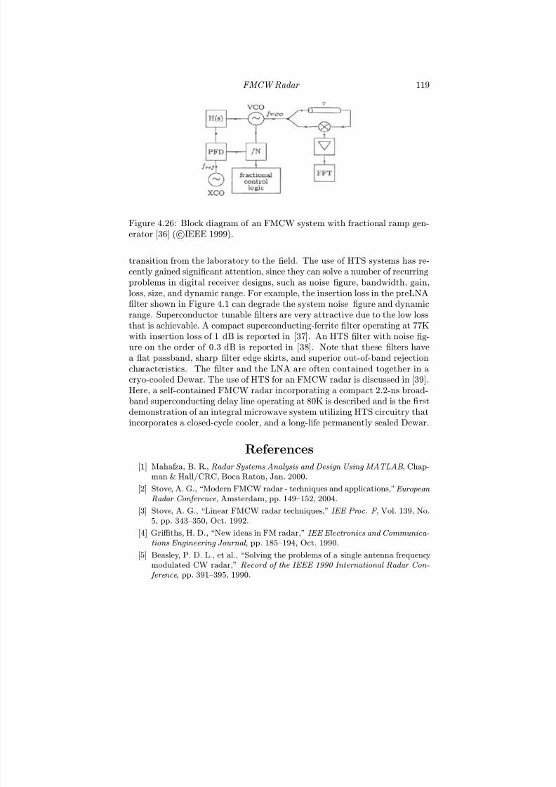
7/17/2019 1596932341 Intercept Radar.pdf
http://slidepdf.com/reader/full/1596932341-intercept-radarpdf 150/891
FMCW Radar 119
Figure 4.26: Block diagram of an FMCW system with fractional ramp gen-erator [36] ( cIEEE 1999).
transition from the laboratory to the field. The use of HTS systems has re-
cently gained signifi
cant attention, since they can solve a number of recurringproblems in digital receiver designs, such as noise figure, bandwidth, gain,loss, size, and dynamic range. For example, the insertion loss in the preLNAfilter shown in Figure 4.1 can degrade the system noise figure and dynamicrange. Superconductor tunable filters are very attractive due to the low lossthat is achievable. A compact superconducting-ferrite filter operating at 77Kwith insertion loss of 1 dB is reported in [37]. An HTS filter with noise fig-ure on the order of 0.3 dB is reported in [38]. Note that these filters havea flat passband, sharp filter edge skirts, and superior out-of-band rejectioncharacteristics. The filter and the LNA are often contained together in acryo-cooled Dewar. The use of HTS for an FMCW radar is discussed in [39].Here, a self-contained FMCW radar incorporating a compact 2.2-ns broad-band superconducting delay line operating at 80K is described and is the first
demonstration of an integral microwave system utilizing HTS circuitry thatincorporates a closed-cycle cooler, and a long-life permanently sealed Dewar.
References
[1] Mahafza, B. R., Radar Systems Analysis and Design Using MATLAB , Chap-man & Hall/CRC, Boca Raton, Jan. 2000.
[2] Stove, A. G., “Modern FMCW radar - techniques and applications,” European
Radar Conference , Amsterdam, pp. 149—152, 2004.
[3] Stove, A. G., “Linear FMCW radar techniques,” IEE Proc. F , Vol. 139, No.5, pp. 343—350, Oct. 1992.
[4] Griffiths, H. D., “New ideas in FM radar,” IEE Electronics and Communica-
tions Engineering Journal , pp. 185—194, Oct. 1990.
[5] Beasley, P. D. L., et al., “Solving the problems of a single antenna frequencymodulated CW radar,” Record of the IEEE 1990 International Radar Con-
ference, pp. 391—395, 1990.
7/17/2019 1596932341 Intercept Radar.pdf
http://slidepdf.com/reader/full/1596932341-intercept-radarpdf 151/891
120 Detecting and Classifying LPI Radar
[6] Nathanson, F. E., and Luke, P. J., “Loss from approximations to square-law detectors in quadrature systems with postdetection integration,” IEEE
Trans. on Aerospace and Electronic Systems, AES-8 pp. 75—77, Jan. 1972.
[7] Filip, A. E. “A baker’s dozen magnitude approximations and their detectionstatistics,” IEEE Trans. of Aerospace and Electronic Systems, AES-12, pp.86—89, Jan. 1976.
[8] Cassandras, C. G., Discrete Event Systems Modeling and Performance Analy-
sis, Aksen and Irwin Associates, Homewood, IL, 1993.
[9] Piper, S. O., “Receiver frequency resolution for range resolution in homo-dyne FMCW radar,” Proc. National Telesystems Conference, Commercial
Applications and Dual-Use Technology, pp. 169—173, 1993.
[10] Piper, S. O., “Homodyne FMCW radar range resolution eff ects with sinu-soidal nonlinearities in the frequency sweep,” Record of the IEEE Interna-
tional Radar Conference, pp. 563—567, 1995.
[11] Turley, M. D. E., “FMCW radar waveforms in the HF band,” ITU-R JRG
1A-1C-8B meeting , Nov. 2006.
[12] Griffiths, H. D., and Bradford, W. J., “Digital generation of high time-bandwidth product linear FM waveforms for radar altimeters,” IEE Proc.
F, Vol. 139, No. 2, pp. 160—169, April 1992.
[13] Pace, P. E., Advanced Techniques for Digital Receivers , Artech House, Inc.,Norwood, MA, July 2000.
[14] Abousetta, M. M., and Cooper, D. C., “Noise analysis of digitized FMCWradar waveforms,” IEE Proc. F , pp. 209—215, Aug. 1998.
[15] Turner, S. E., Chan, R. T., and Feng, J. T., “ROM-based direct digital syn-thesizer at 24 GHz clock frequency in InP DHT technology,” IEEE Microwave
and Wireless Components Letters , Vol. 18, No. 8, pp. 566—568, Aug. 2008.
[16] Liao, S. Y., Microwave Devices and Circuits, 2nd Edition Prentice Hall, Upper
Saddle River, New Jersey, 1980.[17] Harmer, J. D., and O’Hare, W. S., “Some advances in CW radar techniques,”
IRE 5th Mil-E-Con Record , pp. 311—323, 1961.
[18] O’Hara, F. J., and Moore, G. M., “A high p erformance CW receiver usingfeedthrough nulling,” Microwave Journal , Vol. 6, No. 9, pp. 63—71, Sept.1963.
[19] Lin, K., Wang, Y. E., Pao, C.-K., and Shih, Y.-C., “A Ka-Band FMCW radarfront-end with adaptive leakage cancellation,” IEEE Trans. on Microwave
Theory and Techniques , Vol. 54, No. 12, pp. 4041 — 4048, Dec. 2006.
[20] Grajal, J., Asensio, A. and Requejo, L., “From a high-resolution LFM-CWshipborne radar to an airport surface detection equipment,” Proceedings of
the IEEE Radar Conference, pp. 157—160, Madrid, Spain, 2004.
[21] Kim, C.-Y., Kim, J.-G., and Hong, S., “A quadrature radar topology with Txleakage canceller for 24-GHz radar applications,” IEEE Trans. on Microwave
Theory and Techniques, Vol. 55, No. 7, pp. 1438—1444, July 2007.

7/17/2019 1596932341 Intercept Radar.pdf
http://slidepdf.com/reader/full/1596932341-intercept-radarpdf 152/891
FMCW Radar 121
[22] Tujaka, S., “On frequency stability of transmitter in LFMCW MTD radar,”12th International Conference on Microwaves and Radar, MIKON ’98 , Vol.3, pp. 776—780 May 1998.
[23] Fuchs, J., et al., “Simple techniques to correct for VCO nonlinearities in shortrange FMCW radars,” IEEE MTT-S International Microwave Symposium
Digest , pp. 1175—1178, 1996.
[24] Levanon, N., and Getz, B., “Comparison between linear FM and phase-codedCW radars,” IEE Proc. F, Vol. 141, No. 4, pp. 230—240, Aug. 1994.
[25] Jankiraman, M., Wessels, B. J., and van Genderen, P., “Pandora multifre-quency FMCW/SFCW radar,” Record of the IEEE International Radar Con-
ference , pp. 750—757, 2000.
[26] Jankiraman, M., de Jong, E. W., and van Genderen, P., “Ambiguity analy-sis of Pandora multifrequency FMCW/SFCW radar,” Record of the IEEE
International Radar Conference , pp. 35—41, 2000.
[27] Fu, J. S., and Ke, Y., “Anti-jamming aspects of linear FM and phase coded
pulse compressions by simulation,” CIE International Conference of Radar Proc., pp. 605—608, Oct. 8—10, 1996.
[28] Reynolds, L., and Ayasli, Y., “Single chip FMCW radar for target velocityand range sensing applications,” Technical Digest of 11th Annual GaAs IC
Symposium , pp. 243—246, 1989.
[29] Yhland, K., and Fager, C., “A FET transceiver suitable for FMCW radars,”IEEE Microwave and Guided Wave Letters , Vol. 10, No. 9, pp. 377—379,Sept. 2000.
[30] Sasaki, K., et al., “InP MMICs for V-band FMCW radar,” IEEE MTT-S
International Microwave Symposium Digest , pp. 937—940, 1997.
[31] Tessmann, A., et al., “A 77 GHz GaAs pHEMT transceive MMIC for auto-motive sensor applications,” Proc. of the GaAs IC Symposium , pp. 207—210,1999.
[32] Lamberg, J. R., et al., “A compact high performance W-band FMCW radarfront-end based on MMIC technology,” IEEE MTT-S International Microwave
Symposium Digest , pp. 1797—1800, 1999.
[33] Haydl, W. H., et al., “Single-chip coplanar 95 GHz FMCW radar sensors,”IEEE Microwave and Guided Wave Letters , Vol. 9, pp. 73—75, Feb. 1999.
[34] Nalezinski, M., Vossiek, M., and Heide, P., “Novel 25 GHz FMCW front-end with 2.45 GHZ SAW reference path for high precision distance mea-surements,” IEEE MTT-S International Microwave Symposium Digest , pp.185—188, 1997.
[35] Vossiek, M., Kerssenbrock, T. V., and Heide, P., “Novel nonlinear FMCWradar for precise distance and velocity measurements,” IEEE MTT-S Inter-
national Microwave Symposium Digest , pp. 511—514, 1998.
[36] Musch, T., Rolfes, N., and Schiek, B., “A highly linear frequency ramp gen-erator based on a fractional divider phase-locked loop,” IEEE Trans. Instru-
mentation and Measurement , pp. 634—637, April 1999.

7/17/2019 1596932341 Intercept Radar.pdf
http://slidepdf.com/reader/full/1596932341-intercept-radarpdf 153/891
122 Detecting and Classifying LPI Radar
[37] Oates, D. C., Dionne, G. F., and Anderson, A. C., “Magnetically tunablesuperconductor filters,” GOMAC Session 15, Advanced Receiver Technology ,Monterey, CA, pp. 396—399, March 1999.
[38] Terrell, J., “High temperature superconducting filters for military applica-tions,” GOMAC Session 15, Advanced Receiver Technology , Monterey, CA,pp. 400—403, March 1999.
[39] Kapolnek, D. J., et al., “Integral FMCW radar incorporating an HTSC delayline with user-transparent cyrogenic cooling and packaging,” IEEE Trans. on
Applied Superconductivity, Vol. 3 No. 1, pp. 2820—2823, Aug. 1992.
Problems
1. Calculate the error between the envelope detector output xe =
I 2 + Q2
and the envelope approximation detector output (4.1) when I = 1.3 andQ = −3.1 for (a) a = 1, b = 1/2, and (b) a = 1 and b = 1/4.
2. An LPI emitter scans at a rate of 65 deg/s using a triangular FMCWwaveform with modulation period tm = 1 ms. The GOCFAR rangeprocessor sends the report sequence
0, 0, 1, 1, 1, 0, 1, 1, 1, 0, 0, 1, 1, 1, 1, 0, 0, 1, 0, 0, 0, 0, 0
for a target at RT , to a Markov chain with N X = 6 and N Y = 3.Calculate the target’s azimuth extent Θ.
3. An FMCW LPI waveform is shown in Figure 4.27. If the modulationperiod tm = 5 ms, the noise factor F R = 10, and the signal-to-noiseratio required at the receiver output is 13 dB, determine the receiver’ssensitivity in dBmW.
4. For the FMCW waveform shown in Figure 4.27, if the modulation band-width ∆F = 1 GHz, determine the range resolution.
Figure 4.27: FMCW LPI waveform.

7/17/2019 1596932341 Intercept Radar.pdf
http://slidepdf.com/reader/full/1596932341-intercept-radarpdf 154/891
FMCW Radar 123
5. A range resolution of ∆R= 5m is required to contain a ship targetcompletely within a range bin. (a) Calculate the modulation bandwidth∆F required. (b) If the modulation period tm = 1 ms, what is the chirprate required of the radar?
6. Using the results in Section 4.3.2, plot the FMCW magnitude spectrumfor ∆F = 500 kHz and tm = 1 ms.
7. The program lpi fmcw design.m , is useful for understanding FMCWradar systems and can be used to evaluate the trade-off s in the emit-ter design. (a) Use the MATLAB program lpi fmcw design.m to de-sign an FMCW LPI emitter at 9.3 GHz, with an ideal range resolution∆R = 5.5m for a V = 200 m/s target velocity and a maximum targetdistance of 18 km. Choose your modulation period to be tm = 5.5td.Make a table listing the parameters of your design, including: the tar-get’s Doppler frequency; the maximum delay td; the coherent processing
interval; the spectral width; the eff ective transmitted modulation band-width; the degraded resolution, and minimum sampling frequency of the ADC; the FFT size; the adjusted sampling rate of the ADC; themaximum beat frequency; and the time bandwidth product. (b) Whatis the unambiguous range and unambiguous Doppler of your design?
8. The receiver design.m program computes the beat frequencies for a par-ticular target configuration and FMCW radar design (from the programlpi fmcw design.m ). The program asks for the range of the target andthe velocity. Keeping the velocity at 200 m/s, run the program 10 timeswhere, with each iteration, the range is decreased by 1m. For each itera-tion, save both the range-to-the-target and the target velocity computedby the FFT. Plot both of these parameters separately, as a function of
range along with the error (diff erence between the true values and themeasured values). Comment on the size of this error that is computed.
9. If the maximum target velocity is V T = 30 m/s, calculate the requiredmodulation period such that the target moves a maximum of two rangecells during the coherent processing interval. What is the resultingvelocity resolution and spectral width?

7/17/2019 1596932341 Intercept Radar.pdf
http://slidepdf.com/reader/full/1596932341-intercept-radarpdf 155/891

7/17/2019 1596932341 Intercept Radar.pdf
http://slidepdf.com/reader/full/1596932341-intercept-radarpdf 156/891
Chapter 5
Phase Shift KeyingTechniques
In Chapter 4, we discussed the LPI technique of frequency modulation of the CW signal. This chapter presents the phase shift keying techniques thatare useful for LPI radar waveform design. Although not a LPI modulationtechnique, Barker binary PSK is discussed first, since it is the first PSKtechnique to be investigated and is still widely used today. This is followedby a discussion of polyphase shift keying techniques. These include Barkerpolyphase sequences and the Frank code. Also presented are the P1, P2,P3, and P4 codes, and polytime codes T1, T2, T3, and T4. Each of thesecodes is shown to be useful as an LPI CW PSK technique due to its widebandcharacteristics and the fact that it forces the intercept receiver to initially havea large processing gain. For each code, the phase characteristics are examined,
along with the power spectrum magnitude. To quantify the usefulness as aCW LPI waveform, the ACF, PACF, and PAF are examined. As an exampleof a PSK LPI radar, the omnidirectional LPI radar which uses the Frankcode, is discussed.
5.1 Introduction
While linear FMCW has established itself as one of the most popular LPIwaveforms, PSK CW waveforms have recently been a topic of active inves-tigation, due to the their wide bandwidth and inherently low PAF side lobelevels achievable. For the LPI radar (as with pulsed radar), it is importantto have a low side lobe level to avoid the side lobes of large targets frommasking the main peak of smaller targets. The choice of PSK code aff ectsthe radar performance and the implementation. For the PSK waveforms, the
125

7/17/2019 1596932341 Intercept Radar.pdf
http://slidepdf.com/reader/full/1596932341-intercept-radarpdf 157/891
126 Detecting and Classifying LPI Radar
bandwidth (inverse of the subcode period) is selected first by the designer,in order to achieve the range resolution desired. Encompassing a large target(such as a ship) within a single resolution cell can aid in detection, but resultsin a narrow bandwidth signal. On the other hand, a wideband transmittedsignal can be chosen to divide the target echo into many resolution cells, andis a technique that is useful for target recognition. The trade-off here is thatthe radar requires a larger transmitted power to detect a target that has asmall cross section, decreasing the ability of the radar to remain quiet .
Binary phase shifting codes (e.g., 0 or 180 degrees) are popular, but pro-vide little in the way of low side lobes and Doppler tolerance. Most useful forthe LPI radar designer are the polyphase codes where the phase shift valuewithin the subcode can take on many values (not just two) and the codeperiod T can be made extremely long. These codes have better side lobeperformance and better Doppler tolerance than the binary phase codes.1
The PSK techniques can result in a high range resolution waveform, while
also providing a large SNR processing gain for the radar. The average powerof the CW transmission is responsible for extending the maximum detectionrange while improving the probability of target detection (as compared to apulsed signal of equal peak power). PSK techniques are also compatible withnew digital signal processing hardware, and a variety of side lobe suppressionmethods [1—4] can be applied. Compatibility with solid state transmittersenables power management techniques to be used that lower the averagepower requirements of the transmitted CW signal. Power management al-lows the radar to keep a target’s SNR constant within the receiver, as therange to the target changes. An example of this technique is described inChapter 9. In addition, the LPI radar designer can choose from a large se-lection of PSK codes that are available, which is the subject of this chapter.
5.2 The Transmitted Signal
In the PSK radar, the phase shifting operation is performed in the radar’stransmitter, with the timing information generated from the receiver-exciter.The transmitted complex signal can be written as
s(t) = Aej(2πf ct+φk) (5.1)
where φk is the phase modulation function that is shifted in time, accordingto the type of PSK code being used, and f c is the angular frequency of thecarrier. The inphase (I) and quadrature (Q) representation of the complexsignal from the transmitter can be represented as
I = A cos(2πf ct + φk) (5.2)1Doppler tolerance is measured by how well the code compresses in the matched receiver,
when the received signal is Doppler shifted with respect to the reference code.
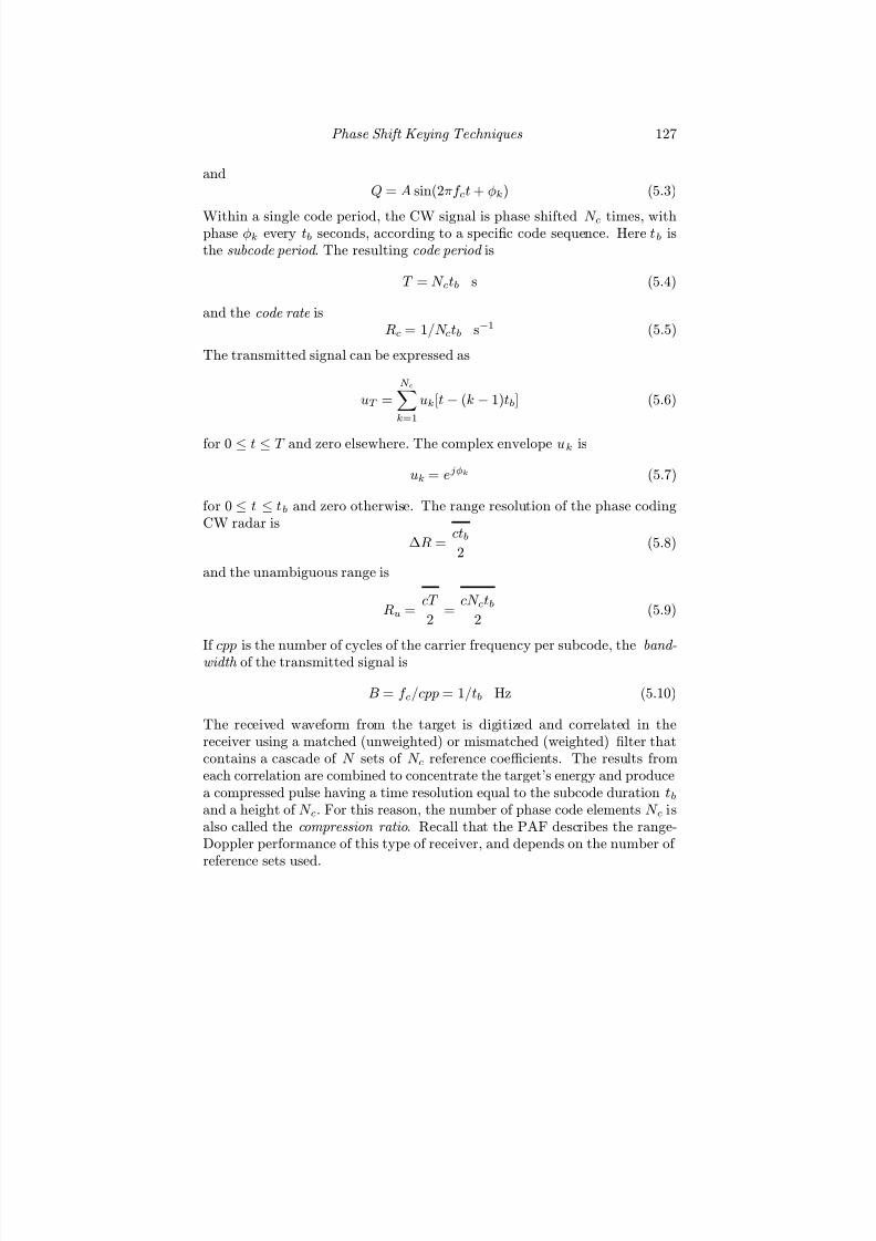
7/17/2019 1596932341 Intercept Radar.pdf
http://slidepdf.com/reader/full/1596932341-intercept-radarpdf 158/891
Phase Shift Keying Techniques 127
andQ = A sin(2πf ct + φk) (5.3)
Within a single code period, the CW signal is phase shifted N c times, withphase φk every tb seconds, according to a specific code sequence. Here tb isthe subcode period . The resulting code period is
T = N ctb s (5.4)
and the code rate isRc = 1/N ctb s−1 (5.5)
The transmitted signal can be expressed as
uT =
N ck=1
uk[t− (k − 1)tb] (5.6)
for 0 ≤ t ≤ T and zero elsewhere. The complex envelope uk is
uk = ejφk (5.7)
for 0 ≤ t ≤ tb and zero otherwise. The range resolution of the phase codingCW radar is
∆R = ctb
2 (5.8)
and the unambiguous range is
Ru = cT
2 =
cN ctb
2 (5.9)
If cpp is the number of cycles of the carrier frequency per subcode, the band-width of the transmitted signal is
B = f c/cpp = 1/tb Hz (5.10)
The received waveform from the target is digitized and correlated in thereceiver using a matched (unweighted) or mismatched (weighted) filter thatcontains a cascade of N sets of N c reference coefficients. The results fromeach correlation are combined to concentrate the target’s energy and producea compressed pulse having a time resolution equal to the subcode duration tb
and a height of N c. For this reason, the number of phase code elements N c isalso called the compression ratio. Recall that the PAF describes the range-Doppler performance of this type of receiver, and depends on the number of reference sets used.

7/17/2019 1596932341 Intercept Radar.pdf
http://slidepdf.com/reader/full/1596932341-intercept-radarpdf 159/891
128 Detecting and Classifying LPI Radar
5.3 Binary Phase Codes
In 1953, R. H. Barker presented binary sequences for synchronization pur-
poses in telecommunications [5]. The binary Barker sequences are finitelength, discrete time sequences with constant magnitude, and a phase of either φk = 0 or φk = π. The formal definition of a Barker sequence is givenbelow [6].
Definition 5.1
A Barker sequence is a finite length sequence A = [a0, a1, . . . , an]of +1’s and −1’s of length n ≥ 2 such that the aperiodic autocor-relation coefficients (or side lobes)
rk =
n−kj=1
aj aj+k (5.11)
satisfies |rk| ≤ 1 for k = 0 and similarly r−k = rk.
Consequently, a binary Barker sequence has elements ai ∈ −1, +1, whichare only known for lengths N c = 2, 3, 4, 5, 7, 11, and 13. A list of the nineknown Barker sequences is shown in Table 5.1 along with their PSL (dB) andISL (dB). The longest code is of length N c=13. The nine sequences are listedwhere a +1 is represented by a + and a −1 is represented by a −. It hasbeen shown that binary Barker sequences with lengths greater than 13, withN c odd, do not exist. Also, it has been proven that binary Barker sequenceswith 4 < N c < 1, 898, 884 with N c even do not exist. It has been conjectured
that sequences with N c ≥ 1, 898, 884 with N c even also do not exist [7].Compound Barker codes (Barker code within a Barker code) can also be
created to have a large compression gain. An example of a compound Barkercode made from a Barker sequence of length N c = 4 is shown in Figure 5.1.Although a larger compression gain is achieved, the peak side lobes are notproportionally decreased. The N c = 169 compound Barker code is frequentlyused and consists of a 13 Barker code inside a 13 Barker code. This representsthe longest binary code sequence from a single concatenation.
The Barker codes are the most frequently used binary code since theyresult in an ambiguity function with side lobe levels, at zero Doppler, nothigher than 1/N c relative to a main lobe of level 1. In fact, due to thisproperty, Barker codes are often called perfect codes . Figure 5.2(a) shows theACF (rk) of a CW signal phase coded with an N c = 13−bit Barker sequence,
and reveals the side lobe structure of the code. For this signal, f c = 1 kHzand the sampling frequency f s = 7 kHz. Note the side lobe characteristicsreflecting the perfect nature of the Barker codes. For the N c = 13−bit code

7/17/2019 1596932341 Intercept Radar.pdf
http://slidepdf.com/reader/full/1596932341-intercept-radarpdf 160/891
Phase Shift Keying Techniques 129
Figure 5.1: A compound N c = 4 Barker code.
Table 5.1: Nine Barker Codes with Corresponding PSL and ISL
Code PSL ISLLength Code Elements (dB) (dB)
2 −+, +− −6.0 −3.03 + + − −9.5 −6.54 + + −+ −12.0 −6.04 + + +− −12.0 −6.05 + + + − + −14.0 −8.07 + + + − − + − −16.9 −9.1
11 + + + − − − + − − + − −20.8 −10.813 + + + + + − − + + − + − + −22.3 −11.5

7/17/2019 1596932341 Intercept Radar.pdf
http://slidepdf.com/reader/full/1596932341-intercept-radarpdf 161/891
130 Detecting and Classifying LPI Radar
Figure 5.2: (a) ACF and (b) PACF for the N c = 13-bit Barker binary PSKsignal (PSL = −22 dB).
shown, PSL = 20 log10(1/N c) = −22.3 dB. The number of cycles per phasecpp = 1. Figure 5.2(b) shows the PACF and reveals the fact that the Barkercodes do not have a perfect PACF side lobe characteristic (zero side lobes),but have a lowest side lobe level that equals the PSL shown for the ACF(−22 dB). In Figure 5.3, a plot of the PAF is shown for N = 1. The delay axisis normalized by the bit period tb so the PAF repeats every τ = N cbsc = 91samples. Note the presence of the large Doppler side lobes.
Upon reception of the target’s return signal, the receiver uses a detector to
generate a + or − for each subcode. Figure 5.4 demonstrates the binary phasecoding technique and receiver architecture using an N c = 13-bit Barker code.In this figure, the receiver output uses a single tapped delay line matchedfilter to compress the transmitted waveform. When the return signal vectoris centered within the filter, the + filter coefficients line up with the signal+’s and − filter coefficients line up with signal −’s, and a maximum outputresults as shown.
In addition to having a limited code length, Barker codes are very sensitiveto Doppler shifts, as illustrated by the large PAF Doppler lobes shown inFigure 5.3. The Doppler shift of the return waveform (due to a motion of thetarget) can compress the waveform within the filter such that the matchedfilter gives incorrect results. This characteristic restricts binary Barker codeapplications. As a final note, Barker codes are not considered LPI since
they are easily detected by an intercept receiver that uses frequency doubling .This simple technique involves multiplying the received signal by itself and

7/17/2019 1596932341 Intercept Radar.pdf
http://slidepdf.com/reader/full/1596932341-intercept-radarpdf 162/891
Phase Shift Keying Techniques 131
Figure 5.3: PAF for 13-bit Barker binary PSK signal showing the largeDoppler side lobes.

7/17/2019 1596932341 Intercept Radar.pdf
http://slidepdf.com/reader/full/1596932341-intercept-radarpdf 163/891
132 Detecting and Classifying LPI Radar
Figure 5.4: Binary phase coding techniques and receiver architecture using a13 Barker code (N c = 13).

7/17/2019 1596932341 Intercept Radar.pdf
http://slidepdf.com/reader/full/1596932341-intercept-radarpdf 164/891
Phase Shift Keying Techniques 133
processing the result with an envelope detector.Barker BPSK signals can easily be generated using the LPIT contained
on the enclosed CD (see Appendix A). The BPSK code generates three typesof CW Barker sequences (N c =7, 11, or 13). Also selectable are the car-rier frequency f c, the sampling frequency f s, the number of code periods togenerate, the cycles per subcode cpp, and the SNR.
5.4 Polyphase Codes
Polyphase sequences are finite length, discrete time complex sequences withconstant magnitude but with a variable phase φk. Polyphase coding refers tophase modulation of the CW carrier, with a polyphase sequence consistingof a number of discrete phases. That is, the sequence elements are takenfrom an alphabet of size N c > 2. Increasing the number of elements orphase values in the sequence allows the construction of longer sequences,
resulting in a high range resolution waveform with greater processing gain inthe receiver or equivalently a larger compression ratio. The trade-off is thata more complex matched filter is required compared to a Barker code filter.Note that a greater sequence length N c does not aff ect the signal bandwidthat the antenna and/or change the transmitted signal bandwidth (B = 1/tb).
Polyphase sequences that satisfy the Barker criteria (so-called polyphaseBarker codes) are currently under investigation in order to try and find longersequences. Polyphase compression codes have also been derived from step-approximation-to-linear-frequency modulation waveforms (Frank, P1, P2)and linear-frequency modulation waveforms (P3, P4). These codes are de-rived by dividing the waveform into subcodes of equal duration, and using aphase value for each subcode that best matches the overall phase trajectoryof the underlying waveform. An alternate approach to approximating thesewaveforms is to quantize the underlying waveform into a user-selected numberof phase states, where the time spent at each phase state changes (in time)throughout the duration of the waveform. These codes are referred to aspolytime codes. Other codes, such as the P (n, k) polyphase codes, have beenderived using a step approximation of the phase function from a nonlinear
frequency modulation waveform with a favorable energy density.The importance of polyphase coding to the LPI community is that by in-
creasing the alphabet size N c, the autocorrelation side lobes can be decreasedsignificantly while providing a larger processing gain. By narrowing the sub-code width tb (so there are fewer cycles per phase), the transmitted signalcan also be spread over a large bandwidth, forcing the receiver to integrateover a larger band of frequencies. Polyphase signals can easily be generated
using the LPIT contained on the enclosed CD (see Appendix A). The usercan select any sequence length, carrier frequency f c, sampling frequency f s,and number of code periods to generate. The cycles per subcode cpp and the

7/17/2019 1596932341 Intercept Radar.pdf
http://slidepdf.com/reader/full/1596932341-intercept-radarpdf 165/891
134 Detecting and Classifying LPI Radar
SNR are also selected.
5.5 Polyphase Barker CodesPolyphase Barker codes allow the LPI emitter a large amount of flexibilityin generating the phase modulated waveforms. Since the number of diff erentphase terms (or alphabet) is not two-valued, there is considerable advantageto their use since they are unknown to the noncooperative intercept receiver.Over the years N c ≤ 63 codes have been discovered and are presented below.
Consider the generalized Barker sequences aj of finite length n wherethe terms aj are allowed to be complex numbers of absolute value 1 where thecorrelation is now the Hermitian dot product2
rk =n−k
j=1
aj a∗
j+k (5.12)
where z∗ represents the complex conjugate of z and the same restrictions inDefinition 5.1 apply (|r(k)| ≤ 1 for k = 0). A class of transformations can bedeveloped that leave the absolute value of the correlation function unaltered,so that, in particular, generalized Barker sequences are changed into othergeneralized Barker sequences [6]. For example, let ur be a complex sequenceof length k and let its autocorrelation function be
rur =
n−τ j=1
uru∗
r+τ (5.13)
Now define a new complex-valued sequence vr of length n as
vr = urej2πr/m (5.14)
where m is any nonzero integer. We can then observe the fact that theautocorrelation function rv
τ satisfies
rvτ =
k−τ r=1
vrv∗r+τ (5.15)
or
rvτ =
k−τ r=1
uru∗
r+τ e−j2πτ /m = ru
τ e−j2πτ /m (5.16)
for all τ . Since |e−j2πτ /m| = 1, |rvτ | = |ru
τ | for all τ Also from (5.13) |vr| = |ur|.
A more general transformation between vr and ur is given in [6].2The Hermitian dot product of two vectors (x1, x2, . . . , xn), (y1, y2, . . . , yn) isn
i=1 xiy
∗
i .

7/17/2019 1596932341 Intercept Radar.pdf
http://slidepdf.com/reader/full/1596932341-intercept-radarpdf 166/891
Phase Shift Keying Techniques 135
Table 5.2: Seven Alternating Quarternary Barker Codes [6]
CodeLength Code Elements
2 +1, + j
3 +1, + j, +14 +1, + j, −1, + j
5 +1, + j, −1, + j, +17 +1, + j, −1, + j, −1, + j, +1
11 +1, + j, −1, + j, −1, − j, −1, + j, −1, + j, −113 +1, + j, −1, − j, +1, − j, +1, − j, +1, − j, −1, + j, +1
Taking m = 4 in (5.13), the sequence (u1, u2, u3, u4 . . . , uk) is trans-formed into (u1, ju2,−u3,− ju4, . . . , (−1)k−1uk) which sets up a one-to-onecorrespondence between ordinary (binary) Barker sequences and four-symbol(±1,± j) Barker sequences in which the real and imaginary terms alternate.This set of sequences is shown in Table 5.2. Note that the alternating Barkersequences of odd length are all palindromic (i.e., read the same forward andbackward) and show a symmetry that is obscured in the binary represen-tation. For a list of all the generalized Barker sequences whose terms arerestricted to the complex sixth roots of unity with N c ≤ 13 the reader isreferred to [6].
Until recently, construction methods for generating N c−phase Barker se-quences with low autocorrelation side lobes were not known and exhaustive
search routines were used. These methods and results are discussed below.In [8] an exhaustive search for all sixth-root Barker sequences was conductedthrough N c = 22, for all eighth-root sequences through N c = 15, and for all12th-root sequences through N c = 15. Table 5.3 shows these results. In theresults, the sequence values ai are rth roots of unity. That is, they are theroots of the polynomial zr − 1 = 0. Their search extended the list of knownBarker sequences up to N c = 19 where the terms of the sequence are sixtiethroots of unity. In Table 5.3, the terms ai are expressed in terms of their phaseangles as multiples of 6 degrees. Their results illustrate the smallest r knownfor each N c where r divides 60.
An iterative algorithm based on constrained iteration techniques is appliedto generate polyphase Barker sequences in [9]. Uniform sequences meeting theBarker condition with N c = 3 up to N c = 25 elements are reported (except
for N c =20 elements). The sequence values ai are shown in Table 5.4.The list of uniform sequences was extended up to N c =31 using the great

7/17/2019 1596932341 Intercept Radar.pdf
http://slidepdf.com/reader/full/1596932341-intercept-radarpdf 167/891
136 Detecting and Classifying LPI Radar
Table 5.3: Polyphase Barker Sequences N c = 1 to 19 [8] ( cIEEE 1989)N c r Sequence ai
1 1 02 1 0 03 2 0 0 304 2 0 0 30 05 2 0 0 0 30 06 6 0 0 10 30 0 407 2 0 0 0 30 30 0
308 6 0 0 0 0 30 20
50 109 3 0 0 0 0 20 40
0 40 2010 6 0 0 0 0 20 40
0 30 10 5011 2 0 0 0 30 30 30
0 30 30 0 3012 6 0 0 10 0 50 20
20 40 0 40 10 30
13 2 0 0 0 0 0 3030 0 0 30 0 300
14 6 0 0 0 10 10 040 40 10 20 40 1050 20
15 4 0 0 0 15 15 045 45 15 30 45 15
0 30 016 12 0 0 0 15 15 0
45 45 15 30 45 150 30 0 35
17 15 0 0 0 4 20 160 48 40 4 28 320 20 4 32 56
18 60 0 0 9 8 53 474 7 35 32 15 37
54 57 35 3 30 819 60 0 0 9 4 16 15
41 3 58 20 43 5731 56 32 28 11 242

7/17/2019 1596932341 Intercept Radar.pdf
http://slidepdf.com/reader/full/1596932341-intercept-radarpdf 168/891
Phase Shift Keying Techniques 137
Table 5.4: Polyphase Barker Sequences N c = 3 to 25 [9] ( cIEE 1989)
N c ai N c ai
3 −0.0121 −1.1943 +0.1409 18 +2.1297 −2.4221 −1.6995 +0.38224 −2.5016 −2.7749 −1.2319 +2.1417 −2.5280 −0.2354 −0.1811 +1.32795 +1.3354 −0.8992 −1.8595 −1.4368 +0.2331 +2.3578 −0.4065 +0.0976
+0.2608 −0.8630 +0.5150 −1.6150 −2.75826 +1.3630 +3.0246 −0.5804 +3.1349 +2.4890 +3.7406
+1.6235 +1.1919 19 −1.9461 +2.6015 −0.0648 −1.30047 +0.8688 +0.9106 −0.9048 −0.6238 +2.1067 +0.5609 +2.4323 −1.6685
+1.7924 +0.0223 +2.6777 −2.7650 −0.4415 +1.6424 −1.46208 −0.3131 −1.2660 +2.8067 +2.6116 −0.4287 +1.5349 +2.3556 +1.0432
−2.9788 −1.4428 +2.1516 −1.8044 +1.1451 +0.3446 +0.72599 −0.6896 −2.6573 +7.2661 −1.0342 20 +0.4786 +0.6706 +1.5770 +1.8712
−0.7098 −1.7158 −0.6370 +1.5811 +2.2135 −2.1501 +0.8608 +1.1924+2.8670 −2.5136 +0.0993 +1.7860 −0.3836
10 −0.5887 −1.8332 +2.1561 −0.3414 −2.8818 +0.0677 −1.3544 −2.4389−1.7728 −0.8423 −1.9530 −0.7544 +2.4420 +2.5909 +1.1860 −0.6338+1.6298 +2.8294 21 +1.8087 +0.7662 −0.5432 −1.5944
11 +2.0760 −0.6452 +2.3212 +1.9586 +1.3209 +0.0701 −0.8463 −1.4062−0.8944 +1.5958 +1.8337 +1.6372 −0.1876 −1.9735 +1.7062 −1.4345−1.2395 −1.1485 −1.6531 −0.0882 +0.2233 +1.3810 +2.8241
12 +2.2363 −2.6854 +3.1305 −2.8078 −1.7205 +2.1529 −2.4726 −0.5451−1.5832 +3.0342 −0.0850 +2.2462 +0.9588+1.9194 −0.6520 −0.3623 −3.0102 22 +2.7208 +2.7943 +2.4522 +2.0044
13 +2.7188 +1.3744 +2.0519 +0.6899 +1.5822 +1.7885 −2.9352 −1.3904+1.6773 −0.2793 +3.0833 +2.2955 −2.1716 −0.9320 +0.8861 +2.2276+0.6941 −2.8756 −1.8306 −0.4901 −1.3843 +0.8799 −2.1043 +2.4527+1.2749 −1.6386 +1.3802 −0.2948 −1.8923
14 −0.7019 −2.2825 +1.2537 −1.4914 +2.6576 +0.6222+2.0131 +2.2090 +1.7266 +2.9683 23 +0.0179 +1.1156 +2.3422 +1.8448+2.5855 +2.4207 −0.6031 +0.1768 +3.1247 −2.6283 −1.4822 +1.2732+2.9666 −2.6327 −2.7484 −1.6192 +2.3777 −0.5946
15 +0.5655 +0.2147 −0.4469 −0.5837 +2.3777 −1.6192 −2.7484 +1.2732−0.9322 +2.6090 +1.0432 −0.8091 −1.4822 −2.6283 +3.1247 +1.8448+1.8799 +2.0924 −2.9651 −0.6062 +2.3422 +1.1156 +0.0179−2.8457 −0.4439 +1.5204 24 +1.4496 −0.3890 −2.1404 +1.4554
16 −0.3146 +0.1656 +0.1834 +0.4540 −1.4167 +2.3177 +0.2333 +0.4296−0.0918 +1.2243 −2.7713 −1.9528 −1.5464 −2.5852 +0.8093 +2.0150
+0.0895 +2.8601 +0.2766 +2.5677 −1.1339 +1.2976 −3.0525 −0.8208−0.1218 −1.1910 −2.9903 +1.6009 −0.8155 −0.1505 +2.1155 +2.6104
17 −1.6448 +0.8837 −2.7783 −0.0189 +2.8658 +3.0213 +2.3375 +2.6871+0.7623 −2.4826 +2.1345 −0.1942 25 +2.6251 +2.9578 +1.8614 +2.4892−2.9279 −2.7891 −2.5196 −0.3109 −1.5638 −0.4785 −1.0745 −0.9767−0.3226 −0.0768 −1.8421 −1.9773 −2.0911 −0.9913 +1.2308 +2.8284−1.9249 −1.3895 −1.5432 −2.6046 +1.4961
−0.1824 −2.7280 −2.8259 −0.1689−2.8375 +0.6143 −2.2693 +1.4167−2.0333

7/17/2019 1596932341 Intercept Radar.pdf
http://slidepdf.com/reader/full/1596932341-intercept-radarpdf 169/891
138 Detecting and Classifying LPI Radar
Table 5.5: Polyphase Barker Sequences N c = 20 to 31 [10] ( cIEE 1994)
N c 20 26 27 28 29 30 31
ai 0.000000 0.000000 0.000000 0.000000 0.000000 0.000000 0.0000000.000000 0.000000 0.000000 0.000000 0.000000 0.000000 0.0000004.553049 0.895841 0.184756 5.463798 0.120401 0.577184 0.4953574.086800 2.043260 0.381913 4.811496 5.552993 0.603685 2.0542632.215325 2.412575 0.501476 3.381014 4.186235 0.587563 2.8808161.894461 4.632634 5.667001 3.739787 4.619877 0.207471 4.1269073.945793 4.659854 5.383231 2.796088 4.174523 5.237221 5.3871503.770581 3.061830 4.897648 4.448612 2.799691 4.913640 5.3227540.092210 2.055563 2.065845 4.248550 5.262097 0.461842 4.1275430.967971 4.540587 1.731439 5.258279 5.715868 0.945976 3.7765332.931040 3.491350 1.958458 4.368063 0.326038 2.715992 5.7135951.003241 2.376147 4.965856 0.595450 5.580307 3.698029 4.8777852.452194 2.690606 3.500713 5.859119 1.481594 4.041807 3.6875153.460843 3.123204 5.477305 2.969228 1.894634 2.346154 4.3135811.330362 1.322308 2.029632 5.908823 3.910927 1.326526 3.3509243.745265 5.951858 5.701172 2.858973 0.109814 5.544522 1.6651171.916620 3.270461 3.226034 5.257347 0.547566 4.813630 0.296297
4.431156 5.356688 0.931898 0.584991 3.212265 1.179540 4.7641312.297439 3.393189 0.153375 4.028262 2.928542 5.217885 0.9208444.416524 1.614152 3.384669 1.763293 1.569419 3.222122 5.779411
3.319561 1.694949 0.929504 5.675662 1.267677 3.9087700.300302 4.205310 4.128530 3.971280 2.683552 5.3012841.920568 5.841580 4.342097 2.537828 0.115401 2.5686184.368801 1.796881 0.824984 5.757173 4.583854 0.3795360.674586 3.989645 1.073402 1.598000 1.642393 4.2869833.485233 5.794346 3.249433 4.602239 4.237597 0.511796
1.622635 4.575381 1.641441 6.267467 2.5396040.561518 4.413265 2.612215 5.184811
1.039439 5.346838 1.0890831.248448 3.330664
0.135490
deluge algorithm (GDA) in [10]. The GDA is a stochastic optimization rou-tine that outperforms other routines such as simulated annealing or thresholdaccepting. First, a quality factor Q is established based on the autocorrela-tion properties. Searching for a global maximum value for the quality factorQ, the GDA allows every phase step size that does not result in a Q valuelower than a certain threshold. During optimization, this threshold is contin-uously increased. The algorithm terminates when the phase step size becomessmaller than a predefined minimum phase step size. These results are shownin Table 5.5 for 20 ≤ N c ≤ 31.
In [11] uniform complex sequences of lengths 32 ≤ N c ≤ 36 are presented.These sequences are also derived using a stochastic optimization algorithm tooptimize a set of continuous phase values after properly selecting the start-ing vectors. After optimization, the phase values are quantized into a finite
alphabet. The results are shown in Table 5.6. Exhaustive search routines arenot feasible for large alphabet sizes. In addition, a suitable initial value forthe quality factors must be chosen. In [12], a systematic method is presented
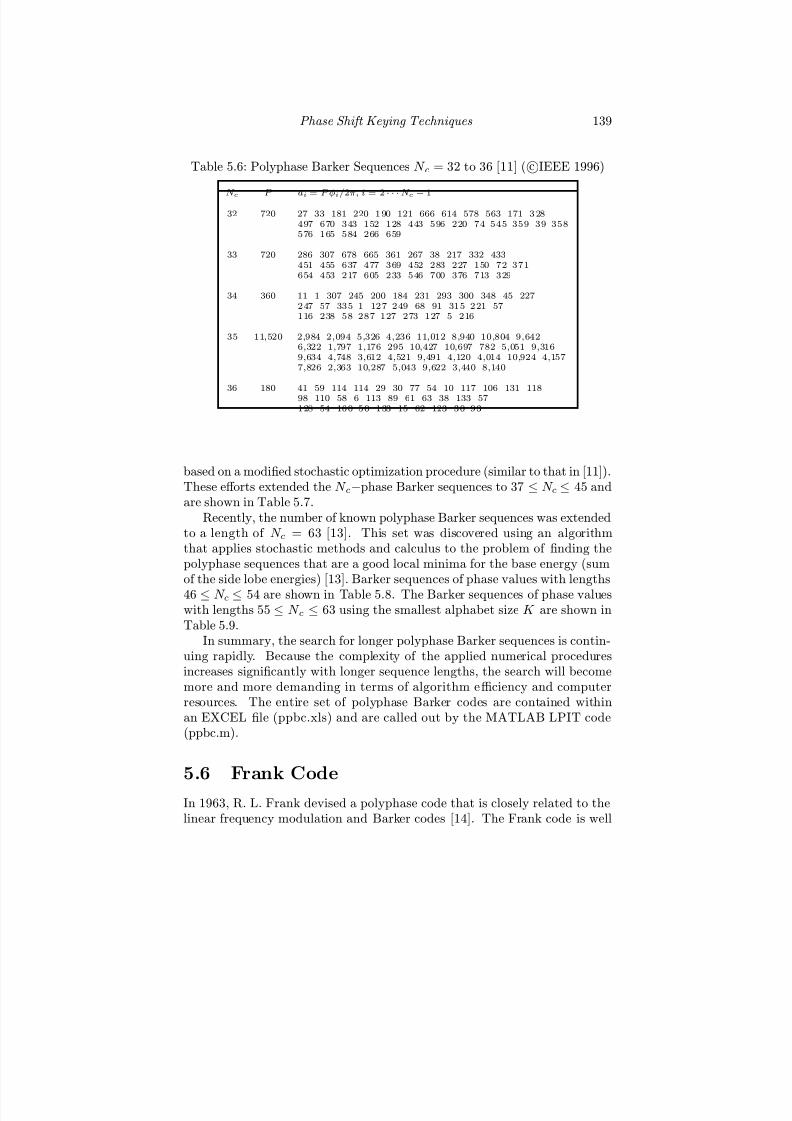
7/17/2019 1596932341 Intercept Radar.pdf
http://slidepdf.com/reader/full/1596932341-intercept-radarpdf 170/891
Phase Shift Keying Techniques 139
Table 5.6: Polyphase Barker Sequences N c = 32 to 36 [11] ( cIEEE 1996)
N c P ai = P φi/2π, i = 2· · ·
N c −
1
32 720 27 33 181 220 1 90 121 666 614 578 563 171 3 28497 670 343 152 128 443 596 220 74 545 359 39 358576 165 584 266 659
33 720 286 307 678 665 361 267 38 217 332 433451 455 637 477 369 452 283 227 150 72 371654 453 217 605 233 546 700 376 713 329
34 360 11 1 307 245 200 184 231 293 300 348 45 2272 47 57 33 5 1 12 7 2 49 68 91 31 5 2 21 57116 238 58 287 127 273 127 5 216
35 11,520 2,984 2,094 5,326 4,236 11,012 8,940 10,804 9,6426,322 1,797 1,176 295 10,427 10,697 782 5,051 9,3169,634 4,748 3,612 4,521 9,491 4,120 4,014 10,924 4,1577,826 2,363 10,287 5,043 9,622 3,440 8,140
36 180 41 59 114 114 29 30 77 54 10 117 106 131 11898 110 58 6 113 89 61 63 38 133 571 28 54 16 0 5 0 1 33 15 62 123 3 0 9 3
based on a modified stochastic optimization procedure (similar to that in [11]).These eff orts extended the N c−phase Barker sequences to 37 ≤ N c ≤ 45 andare shown in Table 5.7.
Recently, the number of known polyphase Barker sequences was extendedto a length of N c = 63 [13]. This set was discovered using an algorithmthat applies stochastic methods and calculus to the problem of finding thepolyphase sequences that are a good local minima for the base energy (sumof the side lobe energies) [13]. Barker sequences of phase values with lengths46 ≤ N c ≤ 54 are shown in Table 5.8. The Barker sequences of phase valueswith lengths 55 ≤ N c ≤ 63 using the smallest alphabet size K are shown inTable 5.9.
In summary, the search for longer polyphase Barker sequences is contin-uing rapidly. Because the complexity of the applied numerical proceduresincreases significantly with longer sequence lengths, the search will becomemore and more demanding in terms of algorithm efficiency and computerresources. The entire set of polyphase Barker codes are contained withinan EXCEL file (ppbc.xls) and are called out by the MATLAB LPIT code(ppbc.m).
5.6 Frank Code
In 1963, R. L. Frank devised a polyphase code that is closely related to thelinear frequency modulation and Barker codes [14]. The Frank code is well

7/17/2019 1596932341 Intercept Radar.pdf
http://slidepdf.com/reader/full/1596932341-intercept-radarpdf 171/891
140 Detecting and Classifying LPI Radar
Table 5.7: Polyphase Barker Sequences N c = 37 to 45 [12] ( cIEE 1998)
N c P ai = P φi/2π, i = 2 · · · N c − 1
37 60 0 0 11 15 20 39 39 54 2 46 37 55 0 4 6 33 55 8 5 4 42 48 2723 13 59 20 3 51 20 59 39 7 29 51 17 30 59 23
38 90 0 0 10 24 28 57 64 71 85 59 5 3 70 84 57 46 74 15 56 1 1 73
3 43 86 6 63 74 44 34 9 9 59 13 78 49 89 54 30 89
39 90 0 0 10 23 21 47 62 58 76 55 6 8 44 59 49 78 26 50 41 8 3 8946 49 1 79 56 52 21 47 2 12 67 72 34 71 35 9 65 29 85
40 90 0 0 7 6 11 14 23 18 83 76 63 53 10 85 47 38 51 19 8 55 285 46 39 58 76 21 20 74 33 59 79 15 45 10 61 13 54 1 41
41 120 0 0 18 2 1 10 1 1 8 32 38 7 4 79 1 11 1 01 6 8 47 2 8 26 0 86 5 2102 101 40 49 98 29 26 78 115 68 22 103 54 104 29 71 6 61117 52
42 120 0 0 3 1 3 12 4 5 58 6 3 75 2 7 26 3 6 44 1 7 109 2 1 51 1 19 5 8117 26 74 12 116 96 67 56 6 14 88 80 5 52 80 22 3 65 11868 27 97 47
43 120 0 0 16 2 5 31 2 1 18 2 4 32 6 5 84 1 18 8 28 1 12 8 6 57 3 3 90119 4 75 63 10 62 75 30 32 6 103 30 91 110 60 101 41 10257 28 91 23 80 21
44 120 0 0 10 3 14 1 9 104 1 02 1 17 9 4 16 2 63 3 9 40 5 5 104 8 4 44118 15 93 82 110 45 22 52 27 99 105 63 31 77 82 16 19 73117 30 94 45 85 12 54
45 90 0 0 7 1 76 71 76 63 56 73 87 9 9 1 4 25 53 62 5 32 35 85 6940 76 57 26 9 83 56 57 21 5 52 89 48 11 68 26 62 6 37 7319 58 12

7/17/2019 1596932341 Intercept Radar.pdf
http://slidepdf.com/reader/full/1596932341-intercept-radarpdf 172/891
Phase Shift Keying Techniques 141
Table 5.8: Barker Sequences 46 ≤ N c ≤ 54 With Alphabet Sizes K ( cIEEE2005)N c K Phase56 190 0, 0, 13, 37, 43, 95, 83, 115, 109, 145, 111, 12, 117, 86, 127, 116, 184, 109,
65, 121, 125, 116, 36, 92, 79, 85, 12, 1, 72, 183, 156, 135, 62, 139, 95, 16,67, 134, 17, 138, 59, 92, 161, 46, 79, 176, 10, 127, 114, 48, 23, 148, 162,88, 117, 35
55 150 0, 0, 8, 18, 18, 19, 22, 105, 100, 127, 119, 128, 117, 118, 53, 33, 112,147, 132, 46, 30, 1, 133, 48, 117, 83, 31, 35, 38, 64, 144, 129, 100, 56, 39,92, 104, 32, 140, 49, 110, 88, 14, 91, 134, 38, 84, 3, 111, 33, 95, 140, 43,
101, 1954 200 0, 0, 23, 43, 16, 9, 40, 51, 20, 7, 67, 126, 178, 180, 71, 120, 144, 151, 61, 25,45, 100, 86, 9, 172, 161, 142, 22, 85, 8, 96, 128, 81, 1, 18, 137, 0, 95, 132, 59,44, 155, 16, 129, 157, 98, 47, 174, 73, 18, 145, 65, 170, 100
53 100 0, 0, 5, 3, 4, 5, 9, 13, 23, 58, 79, 99, 42, 68, 66, 99, 2, 41, 68, 29, 41, 76, 22,25, 94, 98, 74, 59, 16, 58, 35, 62, 22, 93, 85, 19, 54, 17, 56, 94, 64, 92, 43,26, 13, 70, 47, 95, 57, 21, 13, 86, 51
52 185 0, 0, 20, 11, 30, 26, 15, 27, 57, 26, 133, 97, 177, 149, 123, 45, 11, 140, 76,85, 105, 3, 133, 31, 28, 58, 150, 103, 149, 39, 32, 137, 170, 100, 122, 58,42, 86, 2, 172, 50, 128, 163, 49, 136, 76, 122, 17, 20, 108, 171
51 50 0, 0, 4, 4, 18, 20, 27, 25, 25, 26, 24, 15, 15, 14, 9, 32, 36, 2, 21, 17, 9, 27,46, 49, 19, 29, 9, 32, 7, 43, 21, 46, 22, 47, 18, 35, 0, 22, 9, 31, 44, 5, 29, 21,4, 49, 33, 24, 9, 49, 29
50 150 0, 0, 16, 20, 44, 48, 72, 66, 103, 40, 142, 59, 4, 92, 129, 96, 112, 82, 58, 71,94, 67, 1, 52, 58, 112, 92, 37, 14, 59, 107, 3, 68, 146, 71, 102, 40, 58, 0, 124,62, 67, 129, 41, 51, 138, 136, 76, 66, 13
49 90 0, 0, 5, 12, 7, 1, 0, 88, 6, 25, 43, 68, 72, 51, 29, 13, 55, 62, 10, 21, 78, 79, 28,23, 63, 50, 81, 57, 37, 5, 9, 23, 84, 61, 47, 54, 24, 75, 23, 88, 51, 7, 43, 78,35, 65, 15, 51, 7
48 70 0, 0, 1, 5, 14, 23, 35, 36, 26, 22, 17, 5, 68, 16, 16, 51, 53, 0, 21, 13, 63, 50,59, 43, 21, 1, 52, 27, 53, 62, 28, 28, 0, 55, 24, 51, 5, 22, 51, 15, 50, 8, 44, 21,64, 24, 52, 12
47 80 0, 0, 10, 13, 15, 11, 9, 15, 31, 41, 66, 74, 5, 77, 46, 35, 65, 53, 32, 15, 77,59, 37, 30, 42, 4, 8, 39, 74, 71, 25, 57, 60, 24, 54, 23, 41, 75, 19, 58, 13,55, 11, 61, 33, 65, 28
46 90 0, 0, 3, 14, 21, 34, 50, 70, 75, 79, 57, 61, 47, 61, 79, 22, 55, 71, 71, 25, 44,85, 9, 67, 5, 56, 81, 59, 26, 64, 11, 58, 25, 14, 83, 85, 62, 42, 4, 56, 23, 81,50, 24, 11, 71

7/17/2019 1596932341 Intercept Radar.pdf
http://slidepdf.com/reader/full/1596932341-intercept-radarpdf 173/891
142 Detecting and Classifying LPI Radar
Table 5.9: Barker Sequences 55 ≤ N c ≤ 63 with Alphabet Sizes K ( cIEEE2005).
N c K Phase63 2000 0, 0, 88, 200, 250, 89, 1832, 1668, 1792, 145, 308, 290, 528, 819, 1357,
1558, 1407, 1165, 930, 869, 274, 97, 10, 1857, 731, 789, 1736, 150, 1332,1229, 390, 944, 1522, 1913, 648, 239, 1114, 1708, 200, 666, 1870, 1124,1464, 265, 845, 1751, 1039, 53, 737, 1760, 798, 1880, 851, 1838, 1103, 419,1711, 1155, 546, 1985, 1325, 754, 44
62 3000 0, 0, 459, 324, 361, 2987, 152, 432, 2963, 2907, 112, 598, 1276, 1489, 2216,1814, 1505, 2536, 2949, 197, 1039, 1241, 2809, 2780, 1388, 590, 2233, 1352,2458, 2284, 962, 172, 1453, 2245, 799, 558, 2461, 1258, 34, 1666, 2834,1364, 2755, 1369, 2284, 796, 724, 2118, 198, 1327, 2858, 2962, 2021, 1774,
1604, 698, 1059, 100, 2995, 1923, 2278, 88461 1930 0, 0, 58, 1761, 1762, 1703, 1724, 193, 721, 241, 247, 1855, 187, 416,
1379, 1421, 1385, 922, 362, 784, 1401, 1383, 584, 1709, 284, 807, 285, 373,1404, 1739, 1173, 179, 750, 1, 1239, 1215, 1691, 1092, 490, 17, 160, 1047,704, 536, 1515, 820, 1892, 1138, 1630, 139, 288, 1065, 1780, 733, 613,1309, 1452, 550, 1673, 1049, 143
60 210 0, 0, 16, 208, 180, 153, 126, 161, 135, 78, 83, 98, 143, 127, 162, 153, 183,141, 72, 207, 149, 167, 15, 13, 146, 58, 23, 109, 169, 208, 74, 143, 173, 199,51, 50, 31, 142,152, 84, 74, 6, 147, 205, 151, 66, 31, 151, 27, 101, 170, 75,172, 91, 20, 131, 1, 78, 166, 68
59 340 0, 0, 5, 321, 293, 253, 251, 285, 268, 262, 286, 14, 96, 65, 33, 43, 152, 220,235, 71, 142, 49, 262, 176, 285, 31, 181, 150, 305, 337, 108, 138, 13, 209,274, 163, 24, 100, 320, 169, 221, 4, 48, 209, 339, 109, 192, 33, 222, 301, 128,45, 228, 130, 299, 188, 45, 288, 134
58 500 0, 0, 1, 47, 209, 191, 154, 364, 437, 363, 420, 51, 437, 413, 277, 382, 78,4, 428, 267, 308, 352, 238, 115, 205, 179, 474, 425, 234, 52, 443, 311, 482,
491, 400, 234, 297, 495, 492, 169, 397, 464, 75, 259, 476, 121, 437, 183, 34,263, 0, 64, 242, 496, 292, 68, 318, 127
57 240 0, 0, 18, 51, 31, 37, 6, 39, 43, 64, 128, 167, 187, 19, 22, 226, 163, 103, 97,238, 200, 172, 111, 201, 72, 95, 75, 172, 2, 91, 49, 220, 209, 57, 212, 168, 116,206, 110, 102, 25, 131, 2, 30, 143, 182, 42, 107, 216, 89, 10, 161, 29, 170, 106,205, 86
56 190 0, 0, 13, 37, 43, 95, 83, 115, 109, 145, 111, 12, 117, 86, 127, 116, 184, 109,65, 121, 126, 116, 36, 92, 79, 85, 12, 1, 72, 183, 156, 135, 62, 139, 95, 16,67, 134, 17, 138, 59, 92, 161, 46, 79, 176, 10, 127, 114, 48, 23, 148, 162, 88,117, 35
55 150 0, 0, 8, 18, 18, 19, 22, 105, 100, 127, 119, 128, 117, 118, 53, 33, 112,147, 132, 46, 30, 1, 133, 48, 117, 83, 31, 35, 38, 64, 144, 129, 100, 56,39, 92, 104, 32, 140, 49, 110, 88, 14, 91, 134, 38, 84, 3, 111, 33, 95, 140, 43,101, 19
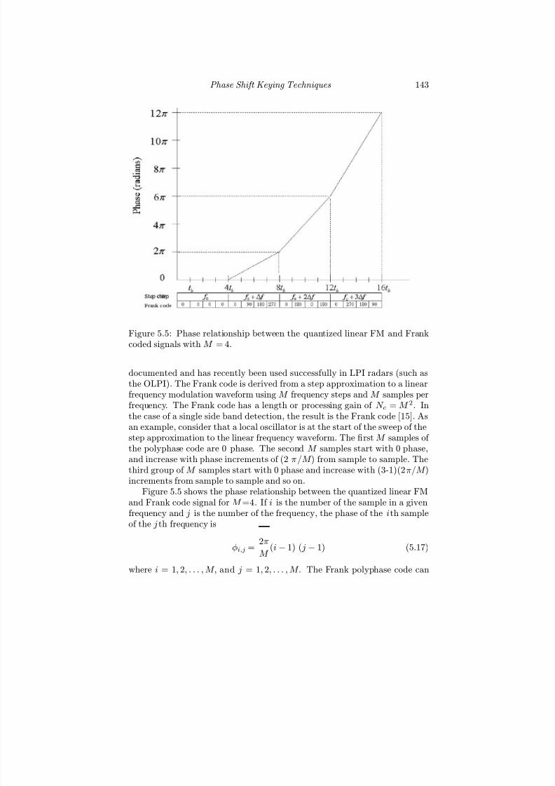
7/17/2019 1596932341 Intercept Radar.pdf
http://slidepdf.com/reader/full/1596932341-intercept-radarpdf 174/891
Phase Shift Keying Techniques 143
Figure 5.5: Phase relationship between the quantized linear FM and Frankcoded signals with M = 4.
documented and has recently been used successfully in LPI radars (such asthe OLPI). The Frank code is derived from a step approximation to a linearfrequency modulation waveform using M frequency steps and M samples perfrequency. The Frank code has a length or processing gain of N c = M 2. In
the case of a single side band detection, the result is the Frank code [15]. Asan example, consider that a local oscillator is at the start of the sweep of thestep approximation to the linear frequency waveform. The first M samples of the polyphase code are 0 phase. The second M samples start with 0 phase,and increase with phase increments of (2 π/M ) from sample to sample. Thethird group of M samples start with 0 phase and increase with (3-1)(2π/M )increments from sample to sample and so on.
Figure 5.5 shows the phase relationship between the quantized linear FMand Frank code signal for M =4. If i is the number of the sample in a givenfrequency and j is the number of the frequency, the phase of the ith sampleof the j th frequency is
φi,j =
2π
M (i− 1) ( j − 1) (5.17)
where i = 1, 2, . . . , M , and j = 1, 2, . . . , M . The Frank polyphase code can

7/17/2019 1596932341 Intercept Radar.pdf
http://slidepdf.com/reader/full/1596932341-intercept-radarpdf 175/891
144 Detecting and Classifying LPI Radar
also be written as an M × M matrix
⎡⎢⎢⎢⎢⎢⎣
0 0 0 · · · 0
0 1 2 · · · (M − 1)0 2 4 · · · 2(M − 1)...
......
...0 (M − 1) 2(M − 1) · · · (M − 1)2
⎤⎥⎥⎥⎥⎥⎦(5.18)
where the numbers represent multiplying coefficients of the basic phase angle2π/M . For the Frank code, the PSL = 20 log10(1/(M π)) [16, 17]. For M =8,N c=64, the PSL = −28 dB.
Figure 5.6(a) shows the discrete phase values that result for the Frankcode for M = 8 (N c = 64). Figure 5.6(b) shows the signal phase modulo 2π,and demonstrates that the Frank code has the largest phase increments fromsample to sample in the center of the code . Consequently, when the Frank
code is passed through a bandpass amplifi
er in a radar receiver, the codeis attenuated most heavily in the center of the waveform. This attenuationtends to increase the side lobes of the Frank code ACF.
Figure 5.7 shows the power spectrum magnitude of a Frank signal withf c =1 kHz, f s =7 kHz, and cpp = 1 with M = 8. Figure 5.7(a) shows thepower spectrum for the signal only, and shows the wideband characteristics(B =1 kHz) resulting from the phase modulation. Figure 5.7(b) shows thepower spectrum for the SNR = 0 dB case. Figure 5.8(a) shows the ACF andthe PACF for the N c = 64 Frank code with N = 1. The ACF reveals thepeak side lobe level PSL = −28 dB. Figure 5.8(b) shows the PACF, and thefact that the Frank code has a perfect PACF. Figure 5.9 shows the PAF forthe Frank code for N c = 64 and N = 1. Note the delay and the Doppler sidelobe levels are much lower than the BPSK code examined in Section 5.3.
Another formulation to generate the Frank code can be found by exam-ining a linear transformation . In a linear transformation of the Frank code,the kth phase element can be expressed as [18]
φk =
2π
M
k − k(mod M )
M [k(mod M )] (5.19)
where M is any positive integer that defines the code sequence length N c =M 2. If the phase-coded signal given in (5.1) is converted into digital formwith a sample period ∆t = tb, then the kth signal sample of the polyphaseFrank code sequence envelope is
sk = A exp[ jφk] = exp
j
2π
M
k − k(mod M )
M k(mod M )
(5.20)
for k = 0, 1, · · · , N c − 1. In a radar application, the sampling rate must behigher. Assuming that the sampling period ∆t = tb/s where s is the number

7/17/2019 1596932341 Intercept Radar.pdf
http://slidepdf.com/reader/full/1596932341-intercept-radarpdf 176/891
Phase Shift Keying Techniques 145
Figure 5.6: Frank code phase values for M = 8 (N c = 64), showing(a) discrete phase jumps and (b) signal phase modulo 2π.

7/17/2019 1596932341 Intercept Radar.pdf
http://slidepdf.com/reader/full/1596932341-intercept-radarpdf 177/891
146 Detecting and Classifying LPI Radar
Figure 5.7: Frank code power spectrum magnitude for M = 8 (N c = 64subcodes) for (a) signal only and (b) SNR = 0 dB.
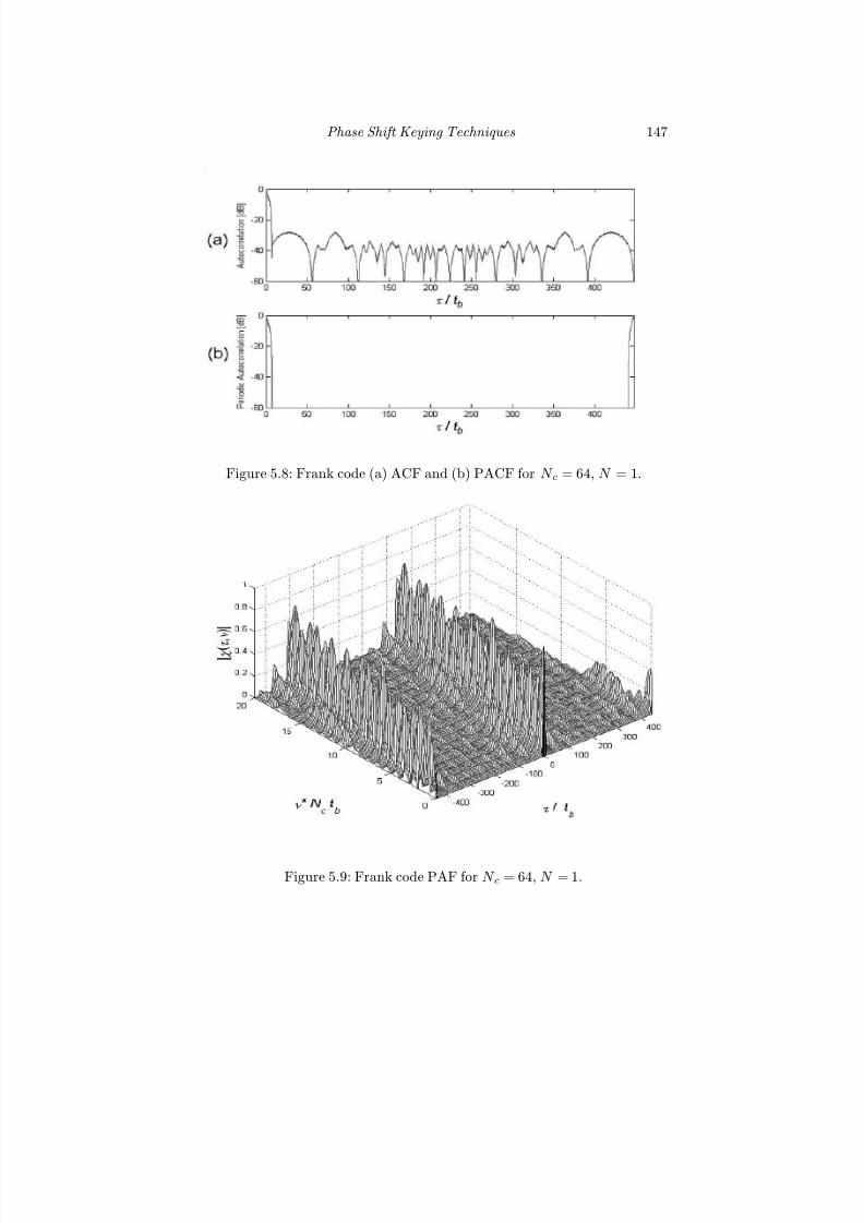
7/17/2019 1596932341 Intercept Radar.pdf
http://slidepdf.com/reader/full/1596932341-intercept-radarpdf 178/891
Phase Shift Keying Techniques 147
Figure 5.8: Frank code (a) ACF and (b) PACF for N c = 64, N = 1.
Figure 5.9: Frank code PAF for N c = 64, N = 1.

7/17/2019 1596932341 Intercept Radar.pdf
http://slidepdf.com/reader/full/1596932341-intercept-radarpdf 179/891
148 Detecting and Classifying LPI Radar
of the samples per subcode, the kth sample of sk is
sk = A exp j
2π
M
k − k(mod M s)
Ms
k − k(mod M s)− (k mod M s) mod s
s
(5.21)where k = 0, 1, . . . , N cs − 1. Note that the influence of the Doppler eff ect isnot taken into consideration with this model.
5.7 P1 Code
The P1 code is also generated using a step approximation to a linear frequencymodulation waveform. In this code, M frequency steps and M samples perfrequency are obtained from the waveform using a double sideband detectionwith the local oscillator at band center [15, 16]. The length of the resultingcode or compression ratio is N c = M 2. If i is the number of the sample in
a given frequency and j is the number of the frequency, the phase of the ithsample of the j th frequency is
φi,j = −π
M [M − (2 j − 1)][( j − 1)M + (i− 1)] (5.22)
where i = 1, 2, . . . , M , and j = 1, 2, . . . , M , and M = 1, 2, 3, . . .. For the P1code the PSL = 20 log10(1/(M π)) (the same as the Frank code).
Figure 5.10(a) shows the phase values that result for the P1 code forM = 8 (N c = 64). Figure 5.10(b) shows the signal phase modulo 2π anddemonstrates that the P1 code has the largest phase increments from sampleto sample at the ends of the code . When the P1 code is passed through thebandpass amplifiers in a radar receiver the attenuation is heaviest on theends of the code. This tends to reduce the side lobes of the P1 AACF in thereceiver [16].3
Figure 5.11 shows the power spectrum magnitude of an f c =1-kHz P1signal (f s =7 kHz, cpp =1) with M = 8, and reveals the wideband natureof this phase modulation. Figure 5.11(a) shows the power spectrum for justthe signal and Figure 5.11(b) shows the power spectrum for the SNR = 0 dBcase.
Figure 5.12(a) shows the ACF and the corresponding side lobe structurefor the N c = 64 P1 code with N = 1. Here PSL = −28 dB down from the peakas predicted. Figure 5.12(b) shows the PACF. Note that the P1 code has aperfect PACF with zero side lobes. Figure 5.13 shows the corresponding PAFfor the P1 code. Note that the PAF repeats at N cbsc = N c(cppf s/f c) = 448samples.
3Recall that the bandpass amplifier attenuation increased the side lobes of the Frankcode AACF.

7/17/2019 1596932341 Intercept Radar.pdf
http://slidepdf.com/reader/full/1596932341-intercept-radarpdf 180/891
Phase Shift Keying Techniques 149
Figure 5.10: P1 code phase values for M = 8 (N c = 64), showing (a) discretephase jumps and (b) signal phase modulo 2π.

7/17/2019 1596932341 Intercept Radar.pdf
http://slidepdf.com/reader/full/1596932341-intercept-radarpdf 181/891
150 Detecting and Classifying LPI Radar
Figure 5.11: P1 code power spectrum magnitude for f c = 1-kHz signal(f s = 7 kHz, cpp = 1) with M = 8 (N c = 64), for (a) signal only and(b) SNR = 0 dB.
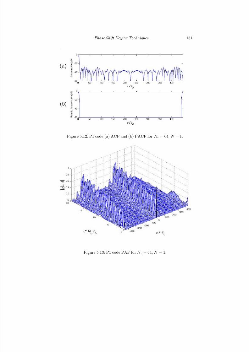
7/17/2019 1596932341 Intercept Radar.pdf
http://slidepdf.com/reader/full/1596932341-intercept-radarpdf 182/891
Phase Shift Keying Techniques 151
Figure 5.12: P1 code (a) ACF and (b) PACF for N c = 64, N = 1.
Figure 5.13: P1 code PAF for N c = 64, N = 1.
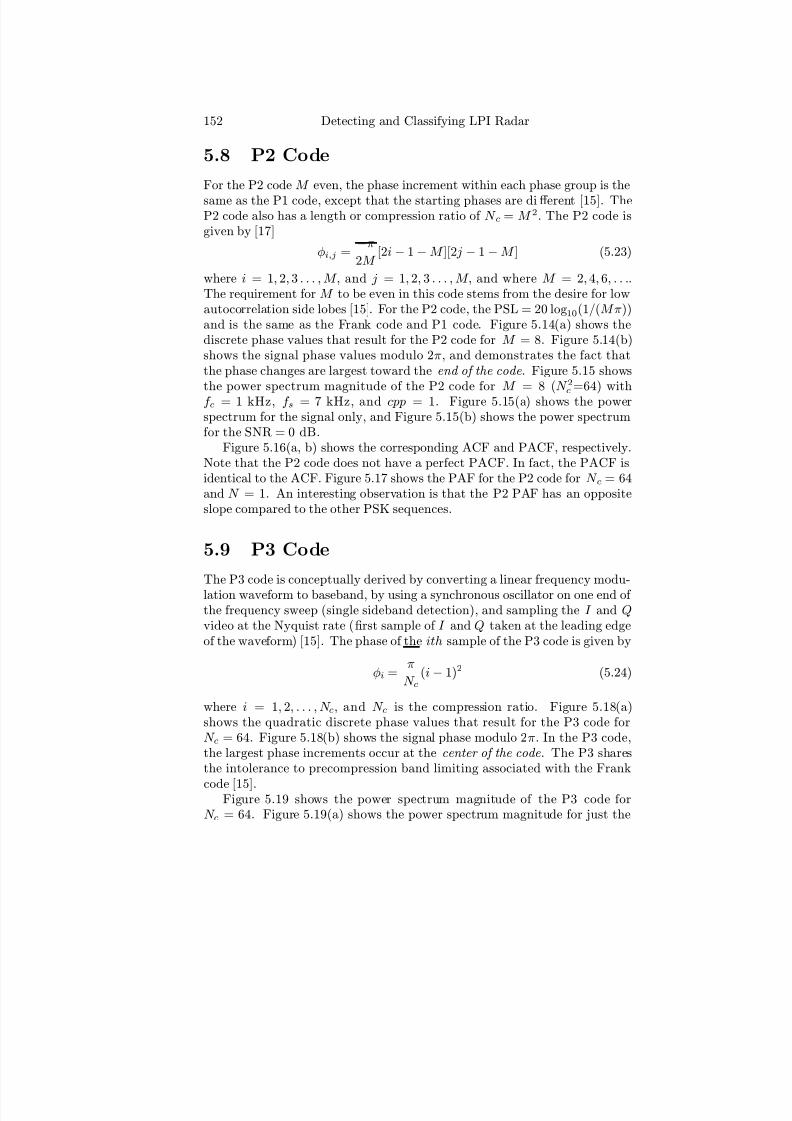
7/17/2019 1596932341 Intercept Radar.pdf
http://slidepdf.com/reader/full/1596932341-intercept-radarpdf 183/891
152 Detecting and Classifying LPI Radar
5.8 P2 Code
For the P2 code M even, the phase increment within each phase group is the
same as the P1 code, except that the starting phases are diff erent [15]. TheP2 code also has a length or compression ratio of N c = M 2. The P2 code isgiven by [17]
φi,j = −π
2M [2i− 1−M ][2 j − 1−M ] (5.23)
where i = 1, 2, 3 . . . , M , and j = 1, 2, 3 . . . , M , and where M = 2, 4, 6, . . ..The requirement for M to be even in this code stems from the desire for lowautocorrelation side lobes [15]. For the P2 code, the PSL = 20 log10(1/(M π))and is the same as the Frank code and P1 code. Figure 5.14(a) shows thediscrete phase values that result for the P2 code for M = 8. Figure 5.14(b)shows the signal phase values modulo 2π, and demonstrates the fact thatthe phase changes are largest toward the end of the code . Figure 5.15 shows
the power spectrum magnitude of the P2 code for M = 8 (N
2
c =64) withf c = 1 kHz, f s = 7 kHz, and cpp = 1. Figure 5.15(a) shows the powerspectrum for the signal only, and Figure 5.15(b) shows the power spectrumfor the SNR = 0 dB.
Figure 5.16(a, b) shows the corresponding ACF and PACF, respectively.Note that the P2 code does not have a perfect PACF. In fact, the PACF isidentical to the ACF. Figure 5.17 shows the PAF for the P2 code for N c = 64and N = 1. An interesting observation is that the P2 PAF has an oppositeslope compared to the other PSK sequences.
5.9 P3 Code
The P3 code is conceptually derived by converting a linear frequency modu-lation waveform to baseband, by using a synchronous oscillator on one end of the frequency sweep (single sideband detection), and sampling the I and Qvideo at the Nyquist rate (first sample of I and Q taken at the leading edgeof the waveform) [15]. The phase of the ith sample of the P3 code is given by
φi = π
N c(i− 1)2 (5.24)
where i = 1, 2, . . . , N c, and N c is the compression ratio. Figure 5.18(a)shows the quadratic discrete phase values that result for the P3 code forN c = 64. Figure 5.18(b) shows the signal phase modulo 2π. In the P3 code,the largest phase increments occur at the center of the code . The P3 sharesthe intolerance to precompression band limiting associated with the Frank
code [15].Figure 5.19 shows the power spectrum magnitude of the P3 code for
N c = 64. Figure 5.19(a) shows the power spectrum magnitude for just the

7/17/2019 1596932341 Intercept Radar.pdf
http://slidepdf.com/reader/full/1596932341-intercept-radarpdf 184/891
Phase Shift Keying Techniques 153
Figure 5.14: P2 code phase values for M = 8 (N 2c = 64), showing (a) discretephase values and (b) signal phase modulo 2π.

7/17/2019 1596932341 Intercept Radar.pdf
http://slidepdf.com/reader/full/1596932341-intercept-radarpdf 185/891
154 Detecting and Classifying LPI Radar
Figure 5.15: P2 code power spectrum magnitude for M = 8, for (a) signalonly and (b) SNR = 0 dB.
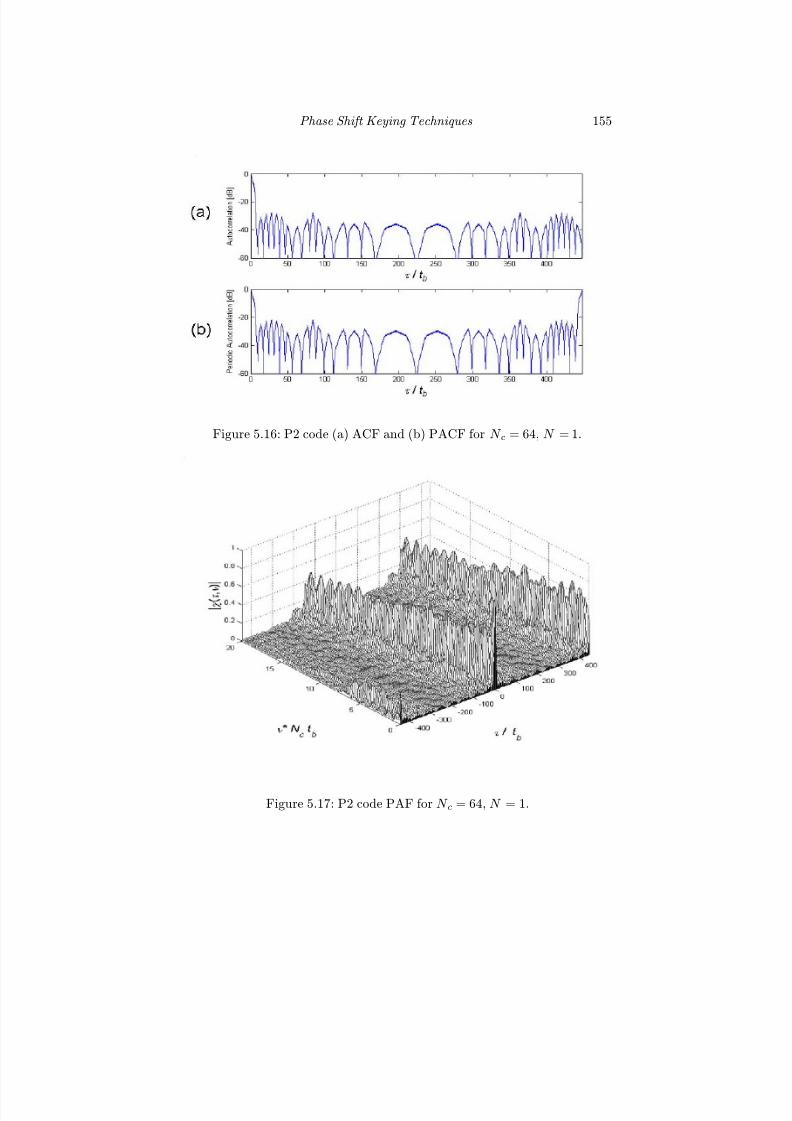
7/17/2019 1596932341 Intercept Radar.pdf
http://slidepdf.com/reader/full/1596932341-intercept-radarpdf 186/891
Phase Shift Keying Techniques 155
Figure 5.16: P2 code (a) ACF and (b) PACF for N c = 64, N = 1.
Figure 5.17: P2 code PAF for N c = 64, N = 1.

7/17/2019 1596932341 Intercept Radar.pdf
http://slidepdf.com/reader/full/1596932341-intercept-radarpdf 187/891
156 Detecting and Classifying LPI Radar
Figure 5.18: P3 code phase values for N c = 64, showing (a) discrete phasesteps and (b) signal phase modulo 2π.

7/17/2019 1596932341 Intercept Radar.pdf
http://slidepdf.com/reader/full/1596932341-intercept-radarpdf 188/891
Phase Shift Keying Techniques 157
signal, and Figure 5.19(b) shows the power spectrum magnitude for the SNR= 0 dB. Figure 5.20(a) shows ACF and the side lobe structure of the P3 forN c = 64 and N = 1. The peak side lobe ratio for the P3 code is larger thanthe Frank, P1, and P2 codes. Here PSL = 20log10
2/(N cπ2) dB, down
from the peak. With N c = 64, PSL = −25 dB. This is revealed in Figure5.20(a) which shows the corresponding ACF. Figure 5.20(b) shows the PACFfor the P3 code and indicates that the P3 has a perfect PACF. The PAF forthe P3 code is shown in Figure 5.21. Here N c = 64 and N = 1. Note thatthe PAF slope for the P3 code is opposite to that of the P2 code.
5.10 P4 Code
The P4 code is conceptually derived from the same linear frequency modu-lation waveform as the P3 code, except that the local oscillator frequency isoff set in the I and Q detectors, resulting in coherent double sideband detec-
tion. Sampling at the Nyquist rate yields the polyphase code named the P4[15, 16]. The P4 code consists of the discrete phases of the linear chirp wave-form taken at specific time intervals, and exhibits the same range Dopplercoupling associated with the chirp waveform. However, the peak side lobe lev-els are lower than those of the unweighted chirp waveform. Various weightingtechniques can be applied to reduce the side lobe levels further. The phasesequence of a P4 signal is described by
φi = π(i− 1)2
N c− π(i− 1) (5.25)
for i = 1 to N c where N c is the pulse compression ratio. Figure 5.22(a)shows the discrete phase values that result for the P4 code for N c = 64.
Figure 5.22(b) shows the signal phase values modulo 2π. The P4 code hasits largest phase increments from sample to sample on the ends of the code ,similar to the P1 code. Figure 5.23(a) shows the power spectrum magnitudefor just the signal, and Figure 5.23(b) shows the power spectrum for the SNR= 0 dB case, and for the P4 code PSL = 20log 10
2/(N cπ2) (same as the
P3 code). Figure 5.24(a) shows the ACF and its corresponding side lobestructure for the N c = 64 P4 code with N = 1. Figure 5.24(b) shows thePACF. The P4 is a Doppler-tolerant perfect code in that it exhibits a perfectPACF—namely zero PACF side lobes.
Figure 5.25 shows the PAF for the P4 code for N c = 64 and N = 1. Notethat the side lobe levels are smaller compared to nonperfect PACF codes,such as the BPSK and P2 code.

7/17/2019 1596932341 Intercept Radar.pdf
http://slidepdf.com/reader/full/1596932341-intercept-radarpdf 189/891
158 Detecting and Classifying LPI Radar
Figure 5.19: P3 code power spectrum magnitude for N c = 64, for (a) signalonly and (b) SNR = 0 dB.

7/17/2019 1596932341 Intercept Radar.pdf
http://slidepdf.com/reader/full/1596932341-intercept-radarpdf 190/891
Phase Shift Keying Techniques 159
Figure 5.20: P3 code (a) ACF and (b) PACF, for N c = 64, N = 1.
Figure 5.21: P3 code PAF for N c = 64, N = 1.

7/17/2019 1596932341 Intercept Radar.pdf
http://slidepdf.com/reader/full/1596932341-intercept-radarpdf 191/891
160 Detecting and Classifying LPI Radar
Figure 5.22: P4 code phase values for N c = 64, showing (a) discrete phasesteps and (b) signal phase modulo 2π.

7/17/2019 1596932341 Intercept Radar.pdf
http://slidepdf.com/reader/full/1596932341-intercept-radarpdf 192/891
Phase Shift Keying Techniques 161
Figure 5.23: P4 code power spectrum magnitude for N c = 64, for (a) signalonly and (b) SNR = 0 dB.

7/17/2019 1596932341 Intercept Radar.pdf
http://slidepdf.com/reader/full/1596932341-intercept-radarpdf 193/891
162 Detecting and Classifying LPI Radar
Figure 5.24: P4 code (a) ACF and (b) PACF, for N c = 64, N = 1.
Figure 5.25: P4 code PAF for N c = 64, N = 1.
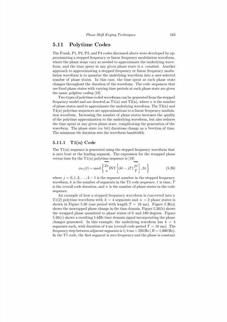
7/17/2019 1596932341 Intercept Radar.pdf
http://slidepdf.com/reader/full/1596932341-intercept-radarpdf 194/891
Phase Shift Keying Techniques 163
5.11 Polytime Codes
The Frank, P1, P2, P3, and P4 codes discussed above were developed by ap-
proximating a stepped frequency or linear frequency modulation waveform,where the phase steps vary as needed to approximate the underlying wave-form, and the time spent at any given phase state is a constant . Anotherapproach to approximating a stepped frequency or linear frequency modu-lation waveform is to quantize the underlying waveform into a user-selectednumber of phase states. In this case, the time spent at each phase statechanges throughout the duration of the waveform. The code sequences thatuse fixed phase states with varying time periods at each phase state are giventhe name polytime coding [19].
Two types of polytime coded waveforms can be generated from the steppedfrequency model and are denoted as T1(n) and T2(n), where n is the numberof phase states used to approximate the underlying waveform. The T3(n) andT4(n) polytime sequences are approximations to a linear frequency modula-tion waveform. Increasing the number of phase states increases the qualityof the polytime approximation to the underlying waveform, but also reducesthe time spent at any given phase state, complicating the generation of thewaveform. The phase state (or bit) durations change as a function of time.The minimum bit duration sets the waveform bandwidth.
5.11.1 T1(n) Code
The T1(n) sequence is generated using the stepped frequency waveform thatis zero beat at the leading segment. The expression for the wrapped phaseversus time for the T1(n) polytime sequence is [19]
φT 1(t) = mod2π
n INT
(kt − jT )
jn
T
, 2π
(5.26)
where j = 0, 1, 2, . . . , k − 1 is the segment number in the stepped frequencywaveform, k is the number of segments in the T1 code sequence, t is time, T is the overall code duration, and n is the number of phase states in the codesequence.
An example of how a stepped frequency waveform is converted into aT1(2) polytime waveform with k = 4 segments and n = 2 phase states isshown in Figure 5.26 (one period with length T = 16 ms). Figure 5.26(a)shows the unwrapped phase change in the time domain. Figure 5.26(b) showsthe wrapped phase quantized to phase states of 0 and 180 degrees. Figure5.26(c) shows a resulting 1-kHz time domain signal incorporating the phasechanges generated. In this example, the underlying waveform has k = 4
segments each, with duration of 4 ms (overall code period T = 16 ms). Thefrequency step between adjacent segments is 1/4 ms = 250 Hz (B = 1,000 Hz).In the T1 code, the first segment is zero frequency and the phase is constant

7/17/2019 1596932341 Intercept Radar.pdf
http://slidepdf.com/reader/full/1596932341-intercept-radarpdf 195/891
164 Detecting and Classifying LPI Radar
Figure 5.26: Stepped frequency waveform generating a polytime code T1(2)showing (a) the unwrapped stepped frequency phase shift, (b) wrapped phasequantized to phase state 0 and 180 degrees, and (c) the resulting time domainwaveform with phase modulation.

7/17/2019 1596932341 Intercept Radar.pdf
http://slidepdf.com/reader/full/1596932341-intercept-radarpdf 196/891
Phase Shift Keying Techniques 165
at zero. The second segment accumulates one full cycle (360 degrees) over theduration of 4 ms. The third segment accumulates an additional two full cycles(720 degrees) over its duration of 4 ms. The fourth segment accumulates anadditional three full cycles (1,080 degrees) over its duration of 4 ms resultingin a total accumulated phase change of 2,160 degrees. As the phase of thestepped frequency waveform crosses increments of 180 degrees, the quantizedphase changes to the alternate state (between 0 degrees and 180 degrees) andremains there until the phase reaches the next 180-degree boundary as shown.
The power spectrum magnitude of the T1(2) signal only is shown in Figure5.27(a). Figure 5.27(b) shows the power spectrum magnitude for the SNR= 0 dB case. These plots serve to demonstrate the wideband nature of thistype of phase modulation. Note that the bandwidth is not equal to B but isthe result of the phase state with the smallest duration.
Figure 5.28(a) shows the ACF and its side lobe structure for the T1(2)code with N = 1. The PSL is high (PSL ≈ −10 dB). From the PACF shown
in Figure 5.28(b), it is clear that the T1(2) also does not have a perfect PACF.Figure 5.29 shows the PAF for the T1(2) code for N = 1. The plot revealsthe high Doppler side lobes expected.
5.11.2 T2(n) Code
The T2(n) sequence is generated by approximating a stepped frequency wave-form that is zero at its center frequency . For stepped frequency waveformswith an odd number of segments, the zero frequency is the frequency of thecenter segment. If an even number of segments is used, the zero frequency isthe frequency halfway between the two centermost segments. The expressionfor the wrapped phase versus time for the T2(n) polytime sequence is
φT 2(t) = mod2π
n INT
(kt − jT )2 j − k + 1
T n
2
, 2π
(5.27)
where the variables are as defined above. An example of how a steppedfrequency waveform is converted into a T2(2) polytime waveform, resultingfrom n = 2 phase states and k = 4 segments, is shown in Figure 5.30 forone period T = 16 ms. Figure 5.30(a) shows the unwrapped phase changein the time domain. Figure 5.30(b) shows the wrapped phase quantized tophase state 0 and 180 degrees. Figure 5.30(c) shows the resulting 1-kHz timedomain signal, illustrating the imposed phase modulation.
The underlying waveform has k = 4 segments, each with duration of 4 ms (overall code period T = 16 ms). The frequency step between adjacentsegments is 1/4 ms= 250 kHz (B = 1,000 Hz). In the T2 code, the phase
shift for the code period is signifi
cantly diff
erent as refl
ected in the unwrappedstepped frequency phase shift and the wrapped phase that is quantized to nphase states.
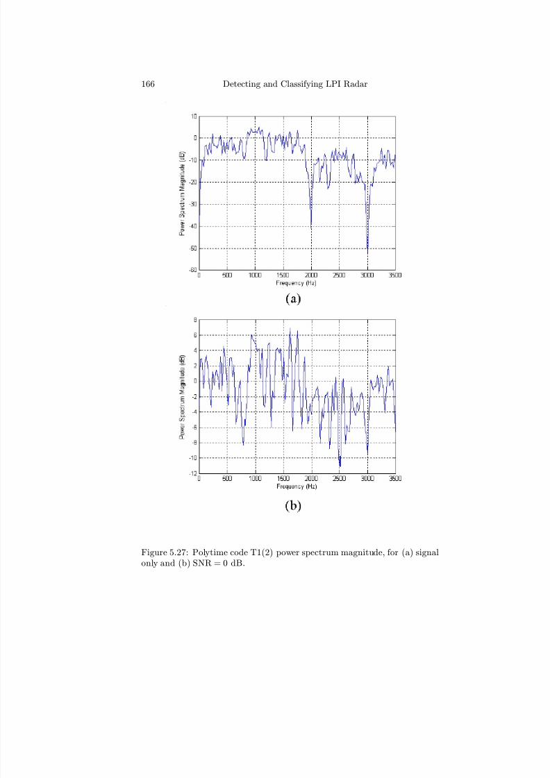
7/17/2019 1596932341 Intercept Radar.pdf
http://slidepdf.com/reader/full/1596932341-intercept-radarpdf 197/891
166 Detecting and Classifying LPI Radar
Figure 5.27: Polytime code T1(2) power spectrum magnitude, for (a) signalonly and (b) SNR = 0 dB.

7/17/2019 1596932341 Intercept Radar.pdf
http://slidepdf.com/reader/full/1596932341-intercept-radarpdf 198/891
Phase Shift Keying Techniques 167
Figure 5.28: T1(2) code (a) ACF and (b) PACF for N = 1.
Figure 5.29: T1(2) code PAF for N = 1.

7/17/2019 1596932341 Intercept Radar.pdf
http://slidepdf.com/reader/full/1596932341-intercept-radarpdf 199/891
168 Detecting and Classifying LPI Radar
Figure 5.30: Stepped frequency waveform generating a polytime code T2(2),showing (a) the unwrapped stepped frequency phase shift, (b) the wrappedphase quantized to phase state 0 and 180 degrees, and (c) the resulting timedomain waveform with imposed phase modulation.

7/17/2019 1596932341 Intercept Radar.pdf
http://slidepdf.com/reader/full/1596932341-intercept-radarpdf 200/891
Phase Shift Keying Techniques 169
The power spectrum magnitude of the T2(2) signal for signal only is shownin Figure 5.31(a), and Figure 5.31(b) shows the power spectrum magnitudefor SNR = 0 dB. Note again, that the bandwidth is not equal to B but is theresult of the phase state with the smallest duration.
Figure 5.32(a) shows the ACF for the T2(2) code with N = 1. Thepeak side lobe level is approximately the same as the T1(2) examined above,except that it occurs at a larger delay (τ /tb = 38). Figure 5.32(b) shows thePACF and reveals that the T2(n) code also does not have a perfect PACF.Figure 5.33 shows the PAF and, as also expected, has fairly large side lobes.
5.11.3 T3(n) Code
A linear FM waveform that is zero beat at its leading edge generates theT3(n). The equation for the wrapped phase versus time for a T3 polytimesequence is
φT 3(t) = mod2π
n INTn∆F t2
2tm
, 2π
(5.28)
where tm is the modulation period and ∆F is the modulation bandwidth.An example of a T3(2) waveform generated using f c =1 kHz, ∆F =1 kHz,and tm =16 ms is given in Figure 5.34. Figure 5.34(a) shows the unwrappedphase change in the time domain. Figure 5.34(b) shows the wrapped phasequantized to phase state 0 and 180 degrees. Figure 5.34(c) shows the resulting1-kHz time domain signal, illustrating the imposed phase modulations. Thequadratic phase accumulates 2,880 degrees after 16 ms. The wrapped phaseshifts between 0 and 180 degrees, as the quadratic phase of the linear FMwaveform passes through increments of 180 degrees.
The power spectrum magnitude of the T3(2) signal only is shown inFigure 5.35(a) and Figure 5.35(b) shows the power spectrum magnitude for
SNR = 0 dB. Figure 5.36(a) shows the ACF for the T3(2) code with N = 1,and indicates that the side lobe performance is somewhat better than theT1(2) or T2(2) code (PSL ≈ −18 dB). Figure 5.36(b) shows the correspond-ing PACF, also indicating that the T3(2) does not have a perfect PACF.Figure 5.37 shows the PAF for the T3(2) code. As expected, the side lobesare relatively high.
5.11.4 T4(n) Code
If the linear frequency modulation waveform is zero beat at its center andis quantized into n discrete phase states, the T4(n) polytime sequence isgenerated. The equation for the wrapped phase versus time for a T4(n)polytime sequence is
φT 4(t) = mod
2π
n INT
n∆F t2
2tm−
n∆F t
2
, 2π
(5.29)

7/17/2019 1596932341 Intercept Radar.pdf
http://slidepdf.com/reader/full/1596932341-intercept-radarpdf 201/891
170 Detecting and Classifying LPI Radar
Figure 5.31: Polytime code T2(2) power spectrum magnitude, for (a) signalonly and (b) SNR = 0 dB.
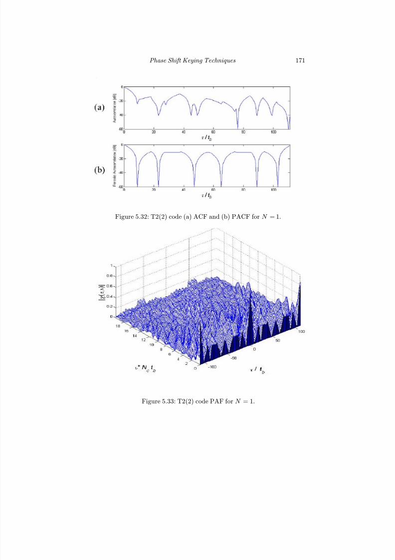
7/17/2019 1596932341 Intercept Radar.pdf
http://slidepdf.com/reader/full/1596932341-intercept-radarpdf 202/891
Phase Shift Keying Techniques 171
Figure 5.32: T2(2) code (a) ACF and (b) PACF for N = 1.
Figure 5.33: T2(2) code PAF for N = 1.

7/17/2019 1596932341 Intercept Radar.pdf
http://slidepdf.com/reader/full/1596932341-intercept-radarpdf 203/891
172 Detecting and Classifying LPI Radar
Figure 5.34: Stepped frequency waveform generating a polytime code T3(2)showing (a) the unwrapped phase shift, (b) the wrapped phase quantized tophase state 0 and 180 degrees, and (c) the resulting time domain waveformwith phase shifts.
7/17/2019 1596932341 Intercept Radar.pdf
http://slidepdf.com/reader/full/1596932341-intercept-radarpdf 204/891
Phase Shift Keying Techniques 173
Figure 5.35: Polytime code T3(2) power spectrum magnitude, for (a) signalonly and (b) SNR = 0 dB.

7/17/2019 1596932341 Intercept Radar.pdf
http://slidepdf.com/reader/full/1596932341-intercept-radarpdf 205/891
174 Detecting and Classifying LPI Radar
Figure 5.36: T3(2) code (a) ACF and (b) PACF for N = 1.
Figure 5.37: T3(2) code PAF for N = 1.

7/17/2019 1596932341 Intercept Radar.pdf
http://slidepdf.com/reader/full/1596932341-intercept-radarpdf 206/891
Phase Shift Keying Techniques 175
An example of a T4(2) waveform with f c =1 kHz, ∆F =1 kHz, and tm =16 msis given in Figure 5.38. Figure 5.38(a) shows the unwrapped phase change inthe time domain. Figure 5.38(b) shows the binary phase code correspondingto each phase shift. Figure 5.38(c) shows the resulting 1-kHz time domainsignal illustrating the phase modulation.
The power spectrum magnitude of the T4(2) signal only is shown inFigure 5.39(a). Figure 5.39(b) shows the power spectrum magnitude forSNR = 0 dB.
Figure 5.40(a) and (b) shows the ACF and PACF, respectively. The T4(2)has side lobes that are higher than the T3(2). The T3(2) also does not havea perfect PACF. Figure 5.41 shows the PAF for the T4(2) code for N = 1,and shows similar performance to the T1(2) through T3(2).
Other sequences can be formed by quantizing the phase into n > 2 phasestates. Increasing the number of phase states increases the quality of thepolytime approximation of the underlying waveform [19]. Since the poly-
time sequences approximate the underlying stepped frequency and linear fre-quency modulation waveforms, it is surprising that their properties do notfollow more closely the properties of the underlying waveform. As more phasestates are added to the polytime sequence, the agreement in time side lobebehavior improves. Polytime coding also has the advantage that arbitrarytime-bandwidth waveforms can be generated with only a few phase states.
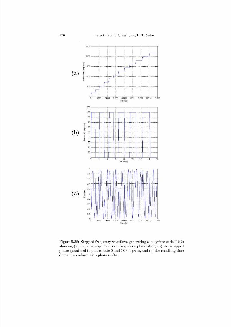
7/17/2019 1596932341 Intercept Radar.pdf
http://slidepdf.com/reader/full/1596932341-intercept-radarpdf 207/891
176 Detecting and Classifying LPI Radar
Figure 5.38: Stepped frequency waveform generating a polytime code T4(2)showing (a) the unwrapped stepped frequency phase shift, (b) the wrappedphase quantized to phase state 0 and 180 degrees, and (c) the resulting timedomain waveform with phase shifts.

7/17/2019 1596932341 Intercept Radar.pdf
http://slidepdf.com/reader/full/1596932341-intercept-radarpdf 208/891
Phase Shift Keying Techniques 177
Figure 5.39: Polytime code T4(2) power spectrum magnitude, for (a) signalonly and (b) SNR = 0 dB.

7/17/2019 1596932341 Intercept Radar.pdf
http://slidepdf.com/reader/full/1596932341-intercept-radarpdf 209/891
178 Detecting and Classifying LPI Radar
Figure 5.40: T4(2) code (a) ACF and (b) PACF for N = 1.
Figure 5.41: T4(2) code PAF for N = 1.
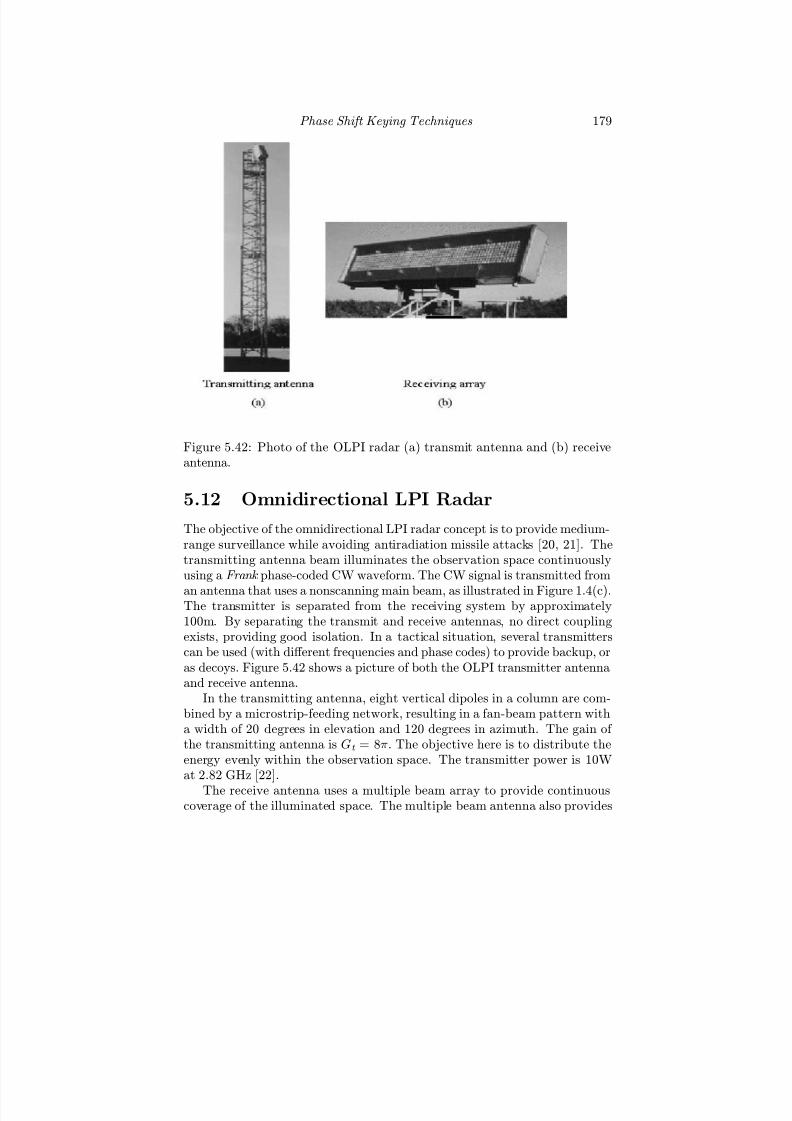
7/17/2019 1596932341 Intercept Radar.pdf
http://slidepdf.com/reader/full/1596932341-intercept-radarpdf 210/891
Phase Shift Keying Techniques 179
Figure 5.42: Photo of the OLPI radar (a) transmit antenna and (b) receiveantenna.
5.12 Omnidirectional LPI Radar
The objective of the omnidirectional LPI radar concept is to provide medium-range surveillance while avoiding antiradiation missile attacks [20, 21]. Thetransmitting antenna beam illuminates the observation space continuouslyusing a Frank phase-coded CW waveform. The CW signal is transmitted from
an antenna that uses a nonscanning main beam, as illustrated in Figure 1.4(c).The transmitter is separated from the receiving system by approximately100m. By separating the transmit and receive antennas, no direct couplingexists, providing good isolation. In a tactical situation, several transmitterscan be used (with diff erent frequencies and phase codes) to provide backup, oras decoys. Figure 5.42 shows a picture of both the OLPI transmitter antennaand receive antenna.
In the transmitting antenna, eight vertical dipoles in a column are com-bined by a microstrip-feeding network, resulting in a fan-beam pattern witha width of 20 degrees in elevation and 120 degrees in azimuth. The gain of the transmitting antenna is Gt = 8π. The objective here is to distribute theenergy evenly within the observation space. The transmitter power is 10Wat 2.82 GHz [22].
The receive antenna uses a multiple beam array to provide continuouscoverage of the illuminated space. The multiple beam antenna also provides

7/17/2019 1596932341 Intercept Radar.pdf
http://slidepdf.com/reader/full/1596932341-intercept-radarpdf 211/891
180 Detecting and Classifying LPI Radar
Figure 5.43: Block diagram of the OLPI radar signal processing.
directional information from the detected targets. The echo from nearbyobjects is strong, while the echo from distant flying targets is weak. Conse-quently, Doppler processing is used to extract the targets from the backgroundclutter. The receive antenna has a planar array of 64 columns, with each col-umn containing eight dipoles combined by a network that is the same as forthe transmit antenna. The total number of antenna elements is 512. Themultiple beams in azimuth are formed by a 64-port Butler matrix that wasmanufactured using microstrip technology. The Butler matrix is an analogbeamforming network, made up of 3-dB directional couplers and fixed phaseshifts, to form N continuous beams with an N element linear array whereN = 2x.
The half-power beamwidth of each beam in the OLPI is 2 degrees, which isalso the azimuth resolution. The gain of the receiving antenna is Gr = 512π.Since everything is illuminated by the transmit antenna, the signals receivedthrough the receive antenna side lobes can pose a problem, making side lobecancelation in the receive beam particularly important.
A block diagram of the OLPI radar signal processing is shown in Figure5.43. The received signal from the Butler matrix is passed through a low-
noise amplifi
er and downconverted to an IF frequency of 30 MHz, fi
ltered,and then converted to baseband I and Q. The ADCs performing the base-band sampling are 12-bit devices sampling at a rate of 250 kHz. The received
7/17/2019 1596932341 Intercept Radar.pdf
http://slidepdf.com/reader/full/1596932341-intercept-radarpdf 212/891
Phase Shift Keying Techniques 181
signals for each resolution are integrated during a time of T s=2s. The rangeresolution is matched to the azimuth resolution at 30 km, which is 600m.Therefore, the range resolution is 600m, resulting in a subcode width of tb = 4 μs. With f s = 250 kHz, each subcode period contains one I andQ pair. The Frank code length is N c = 64, resulting in a code period of T = 256 μs and is equivalent to an Ru =38.4 km.
The first step in the signal processing is to suppress the (mostly stationary)clutter echoes, using a recursive notch filter. After clutter suppression, thecode compression is accomplished by using an FFT that efficiently compressesthe Frank code. The processing gain due to code compression is N c = 64.Because the phase is unknown, however, there is a loss of 1 dB comparedto fully coherent integration resulting in a net processing gain of P GR =10log10(N c) − 1 or 17 dB.
The phase code compression is followed by Doppler filtering to extract themoving targets. To detect targets with velocity v =250m/s at 38 km within
an integration time of T s = 2s, the resulting Doppler spectral width is
∆ω = 2∆v
λ =
2v2T sRλ
(5.30)
or 60 Hz. The filter width is matched to this value, resulting in a coherentintegration time of 16 ms and corresponds to 64 code periods, each 256 μslong. That is, 64 code periods are integrated for each range bin.
To simplify the hardware complexity of having to process 4,096 range bins,the signal is digitized into a single bit (±1) [22]. The processing gain due tothe Doppler filtering of 64 phase codes is P G = 10log10(64) = 18 dB. Dueto the digitization into a single bit, however, a loss of 2 dB is encountered.Also, since the Doppler frequency and phase are unknown, an additional lossof 2.5 dB is included, resulting in a processing gain due to Doppler filtering
of P GR = 18− 2.5− 2 = 13.5 dB.The fourth step described in [22] is the noncoherent integration of theoutputs of the Doppler filter bank. The noncoherent integration is carriedout over the frame time (T = 2s). During the total integration time of T s = 2s, a further 128 signals are integrated in amplitude individually. With64 beams, 64 range bins, and 64 Doppler filters per range bin, a total of 262,144 resolution cells are available. The processing gain due to noncoherentintegration is 12.7 dB. The total processing gain for all three stages is thenP GR = 17 + 13.5 + 12.7 =43.2 dB. With an output detection threshold of SNRRo = 13 dB, the required input SNRRi = −30.2 dB. With BRi = 1/tb =250 kHz and F R = 5.6 dB (including Butler matrix loss), the sensitivity of the OLPI can be estimated as
δ R = kT 0F RBRiSNRRi =
−174 dBW (5.31)
The OLPI radar has been used experimentally to detect hovering helicopters(above terrain masking for only a short time), and is described more fully

7/17/2019 1596932341 Intercept Radar.pdf
http://slidepdf.com/reader/full/1596932341-intercept-radarpdf 213/891
182 Detecting and Classifying LPI Radar
in [22]. Although the OLPI is only one example of an LPI radar that usesphase modulation, there have also been others built that use much longerphase codes such as the Hughes Aircraft Company “quiet radar” built in theearly 1980s.
5.13 Summary
In this chapter we have examined several popular PSK LPI radar schemes,as well as some new techniques recently developed. The phase structure wasexamined for each type of code, along with an analysis of the magnitude of phase change throughout the code. The power spectrum results were alsopresented. The correlation and ambiguity functions from Chapter 3 wereused to examine each waveform’s ACF, PACF, and PAF in order to determineits suitability for use as an LPI waveform. In the next chapter we look atfrequency shift keying techniques for LPI radar applications, as well as hybrid
FSK/PSK techniques.
References
[1] Lee, W. K., and Griffiths, H. D., “Pulse compression filter generating optimaluniform range sidelobe level,” IEE Electronics Letters , Vol. 35, No. 11, pp.873—875, May 1999.
[2] Lee, W. K., Griffiths, H. D., and Benjamin, R., “Integrated sidelobe energyreduction technique using optimal polyphase codes,” IEE Electronics Letters ,Vol. 35, No. 24, pp. 2090—2091, Nov. 1999.
[3] Grishin, Y. P., and Zankiewicz, A., “A neural network sidelobe suppressionfilter for a pulse—compression radar with powers-of-two weights,” IEEE 10th
Mediterranean Electrotechnical Conference , Vol. 2, pp. 713—716, 2000.[4] Lee, W-K., and Griffiths, H. D., “A new pulse compression technique gener-
ating optimal uniform range sidelobe and reducing integrated sidelobe level,”Record of the IEEE International Radar Conference , pp. 441—446, 2000.
[5] Barker, R. H., “Group synchronizing of binary digital systems,” in Commu-
nications Theory , Butterworth, London, pp. 273—287, 1953.
[6] Golomb, S. W., and Scholtz, R. A., “Generalized Barker sequences,” IEEE
Trans. on Information Theory, Vol. IT-11, No. 4, pp. 533—537, Oct. 1965.
[7] Eliahou, S., and Kervaire, A., “Barker sequences and diff erence sets,” L’
Enseignement Mathematique, Vol. 38, pp. 345—382, 1992.
[8] Zhang, N., and Golomb, S. W., “Sixty-phase generalized Barker sequences,”IEEE Trans. on Information Theory, Vol. 35, No. 4, pp. 911—912, April
1989.[9] Bomer, L., and Antweiler, M., “Polyphase Barker sequences,” IEE Electronics
Letters, Vol. 25, No. 23, pp. 1577—1579, 1989.

7/17/2019 1596932341 Intercept Radar.pdf
http://slidepdf.com/reader/full/1596932341-intercept-radarpdf 214/891
Phase Shift Keying Techniques 183
[10] Friese, M., and Zottmann, H., “Polyphase Barker sequences up to length 31,”IEE Electronics Letters , Vol. 30, No. 23, pp. 1930—1931, Nov. 1994.
[11] Friese, M., “Polyphase Barker sequences up to length 36,” IEEE Trans. on Information Theory, Vol. 42, No. 4, pp. 1248—1250, July 1996.
[12] Brenner, A. R., “Polyphase Barker sequences up to length 45 with smallalphabets,” IEE Electronics Letters, Vol. 34, No. 16, pp. 1576—1577, Aug.1998.
[13] Borwein, P., and Ferguson, R., “Polyphase sequences with low autocorrela-tion,” IEEE Trans. on Information Theory, Vol. 51, No. 4, pp. 1564—1567,April 2005.
[14] Frank, R. L., “Polyphase codes with good nonperiodic correlation properties,”IEEE Trans. IT-9, pp. 43—45, 1963.
[15] Lewis, B. L., Kretschmer, F. F., and Shelton, W. W., Aspects of Radar Signal
Processing, Artech House, Norwood, MA, 1986.
[16] Lewis, B. L., “Range-time-sidelobes reduction technique for FM-derived poly-phase PC codes,” IEEE Trans. on Aerospace and Electronic Systems, Vol.29, No. 3, pp. 834—840, July 1993.
[17] Painchaud, G. R., et al., “An experimental adaptive digital pulse compres-sion subsystem for multi-function radar applications,” Record of the IEEE
International Radar Conference, pp. 153—158, 1990.
[18] Lesnik, C. J., et al., “Efficient matched filtering of signal with polyphaseFrank coded sequences,” IEEE 12th International Conference on Microwaves
and Radar , MIKON ’98 , Krakow, Poland, Vol. 3, pp. 815—819, May 20—22,1998.
[19] Fielding, J. E., “Polytime coding as a means of pulse compression,” IEEE
Trans. on Aerospace and Electronic Systems , Vol. 35, No. 2, pp. 716—721,Apr. 1999.
[20] Wirth, W. D., “Long term coherent integration for a floodlight radar,” Record of the IEEE International Radar Conference , pp. 698—703, 1995.
[21] Wirth, W. D., “Polyphase coded CW radar,” Proc. of the IEEE Fourth
International Symposium on Spread Spectrum Techniques and Applications ,Mainz, Germany, Vol. 1, pp. 186—190, Sept. 22—25, 1996.
[22] Wirth, W. D., Radar Techniques Using Array Antennas, IEE, London, UnitedKingdom, 2001.
Problems
1. For an LPI CW radar with an f c =9 GHz, (a) what is the subcodeperiod tb of the transmitted waveform if the cycles per subcode cpp = 5?
(b) What is the transmitted bandwidth of the signal? (c) If the numberof phase codes used is N c = 128, what is the code rate Rc and the rangeresolution?

7/17/2019 1596932341 Intercept Radar.pdf
http://slidepdf.com/reader/full/1596932341-intercept-radarpdf 215/891
184 Detecting and Classifying LPI Radar
Figure 5.44: LPI phase-coded waveform.
2. The generation of an LPI phase-coded CW signal is shown inFigure 5.44. If the carrier frequency is 0.5 MHz, (a) what is the codeperiod (in seconds)? (b) What is the unambiguous range of the wave-form (in km)? (c) What is the bandwidth of the transmitted signal(in MHz)? (d) What is the range resolution of the waveform (in m)?(e) If the phase code used is a P3 or P4 code, what would you expectthe ACF peak side lobe level to be (in decibels down from the mainlobe response)?
3. (a) Using the bpsk.m file as a template, generate a compound Barkercode with f c = 1 kHz, cpp = 2, and N c = 7. (b) Add this capabilityto the LPIT menu. (c) For this waveform, how many subcodes arecontained within a code period? (d) What is the subcode period tb?(e) Plot the ACF, PACF, and the PAF. (f) What can you say aboutthe PSL and the Doppler side lobe levels?
4. (a) Generate three code periods of an f c = 1 kHz (f s = 7 kHz), cpp = 3polyphase Barker code with length N c = 16. (b) Plot the ACF, PACF,
and PAF. (c) Compare these results with an f c =1 kHz (f s = 7 kHz),cpp = 3 polyphase P4 code with length N c = 16.
5. Use the lpit.m file in the LPIT toolbox to generate the default BPSK,Frank, P1—P4 and T1—T4 codes, and both test signals by selecting the“no change” option for each signal to accept the defaults. Be sure to
write down the default parameters for each case. The signals will besaved automatically to your LPIT directory. Move these signals to aseparate folder for use in Part II of this text.
6. Run the LPIT and select the BPSK signal. (a) Change only the num-ber of cycles per Barker bit to 1 (cpp = 1), and generate the sig-nal. That is, each bit now contains only 1 cycle of the IF frequency.
(b) Plot the power spectrum magnitude and record the approximate3-dB bandwidth of the waveform, comparing this with a calculation of what you would theoretically expect. (c) Repeat for cpp = 7.
7/17/2019 1596932341 Intercept Radar.pdf
http://slidepdf.com/reader/full/1596932341-intercept-radarpdf 216/891
Phase Shift Keying Techniques 185
7. Consider a generalized Barker sequence with the general transformation
vr = urej2π(r+α)/x
where α and x are any real numbers, x = 0 with |vr| = |ur| and |rvτ |
|ruτ |. Show that the transformation vr = uk−r+1 preserves the Barker
property and runs the sequence backwards.
8. (a) Using the LPIT toolbox, generate polytime codes T1(8) and T2(8),with f c = 1 kHz, f s = 7 kHz, k = 4, and tm = 16 ms. (b) Plotthe phase distribution within a code period for each signal. (c) Plotthe ACF, PACF, and PAF for each signal. (d) Compare the phasedistribution diagrams with those shown in Figure 5.26 and Figure 5.30.(e) Compare the correlation and ambiguity diagrams with those shownin Figure 5.28(a, b), Figure 5.29, Figure 5.32(a, b), and Figure 5.33.
9. (a) Using the LPIT toolbox, generate polytime codes T3(8) and T4(8),with f c = 1 kHz, f s = 7 kHz, k = 4, ∆F = 1 kHz, and tm = 16 ms.(b) Plot the phase distribution within a code period for each signal. (c)Plot the ACF, PACF, and PAF for each signal. (d) Compare the phasedistribution diagrams with those shown in Figure 5.34 and Figure 5.38.(e) Compare the correlation and ambiguity diagrams with those shownin Figure 5.36(a, b), Figure 5.37, Figure 5.40(a, b), and Figure 5.41.
10. (a) Determine the maximum detection range of the OLPI radar for aσT = 5 m2 target if the losses total 14 dB. (b) How does this rangecompare with Ru?

7/17/2019 1596932341 Intercept Radar.pdf
http://slidepdf.com/reader/full/1596932341-intercept-radarpdf 217/891

7/17/2019 1596932341 Intercept Radar.pdf
http://slidepdf.com/reader/full/1596932341-intercept-radarpdf 218/891
Chapter 6
Frequency Shift Keying
Techniques
CW waveforms with pulse compression allow the LPI radar to have a signif-icant processing gain over an unintended intercept receiver, due to the codesecrecy and the large bandwidth signals that are transmitted. In Chapter4, it was shown that an FMCW waveform is the simplest technique to im-plement, with the compression of the waveform done using either analog ordigital hardware. In Chapter 5, PSK techniques were shown to have signif-icant promise, due to advances in digital hardware and the fact that manycodes and code lengths are available to choose from. Another coding tech-nique that increases the library of LPI radar waveforms is the use of frequency
shift keying . In this chapter three important FSK or frequency hopping (FH)techniques for coding CW waveforms are presented.
6.1 Advantages of the FSK Radar
Much of the LPI radar technology fielded today is linear FMCW, with thesimplicity of this technology being its main advantage.1 The FMCW ap-proach spreads the transmitted energy out over the modulation bandwidthto eff ectively reduce the power spectral density (PSD). The main disadvan-tage, as illustrated in Chapter 4, is the high side lobe values that occur onthe order of 13 dB down from the peak response, and so this type of wave-form requires that some type of weighting be applied to the matched filter
response. The PSK radar uses polyphase codes to reduce the side lobe lev-els, and the waveforms are directly compatible with digital generation and
1A review of fielded LPI radar systems is given in Chapter 2.
187

7/17/2019 1596932341 Intercept Radar.pdf
http://slidepdf.com/reader/full/1596932341-intercept-radarpdf 219/891
188 Detecting and Classifying LPI Radar
compression, making their use more attractive. In addition, the codes mustbe chosen carefully in order to maintain Doppler tolerance.
An LPI radar that uses FH techniques hops or changes the transmittingfrequency in time over a wide bandwidth in order to prevent an unintendedreceiver from intercepting the waveform.2 The frequency slots used are cho-sen from an FH sequence , and it is this unknown sequence that gives theradar the advantage in terms of processing gain. That is, the frequency se-quence appears random to the intercept receiver, and so the possibility of itfollowing the changes in frequency is remote. This prevents a jammer fromreactively jamming the transmitted frequency.3 In contrast to the FMCWand PSK techniques, the FH technique of rapidly changing the transmitterfrequency does not lower the PSD of the emission, but instead moves thePSD about according to the FH sequence. Consequently, the FH radar has ahigher probability of detection than a PSK or FMCW waveform, but retainsa significantly low probability of interception.
In a PSK radar, all the control circuitry, modulators, and demodulatorsmust have enough bandwidth in order to avoid transmitting second ordereff ects, thereby making the overall system expensive [1]. A major advan-tage of the FH radar is the simplicity of the FSK architecture, especially fortrack processing and generating large bandwidth signals. Large bandwidthfrequency hopping radar waveforms can be generated by using coherent di-rect analog synthesizers that generate the output frequencies using standardVCOs and very simple digital circuitry. Drawbacks of this approach includespurious frequencies and high levels of phase noise, due to the complex analogcircuitry required. Direct digital methods can also be used, and involve using
a digital frequency synthesizer and a digital-to-analog converter, followed bya lowpass filter. The major disadvantage here is that the output bandwidthis limited by the speed of the digital devices. Single or multiple phaselockedloops can also be used and have the advantage of large bandwidths and theability to filter spurious frequencies outside the loop bandwidth [2].
Another advantage of the FH radar is that the range resolution is in-dependent of the hopping bandwidth (unlike that of the FMCW and PSKtechniques). Range resolution in an FH radar depends only on the hop rate .A significant benefit also resides in the secrecy of the FH sequence that isused. FH radar performance depends only slightly on the code used, giventhat certain properties are met. This allows for a larger variety of codes,making it more difficult to intercept. By comparison, a PSK radar mustchoose from a group of well-known codes, due to the ambiguity properties
2A frequency hopping radar is diff erent than a frequency agile radar, in that the fre-
quency agile radar is usually regarded as a pulse radar that uses a diff erent frequency on a
pulse-to-pulse basis. The LPI frequency hopping radar transmits a CW frequency hopped
signal.3A jammer can preemptively jam a FH radar if its bandwidth and power are large enough
to cover the FH band.
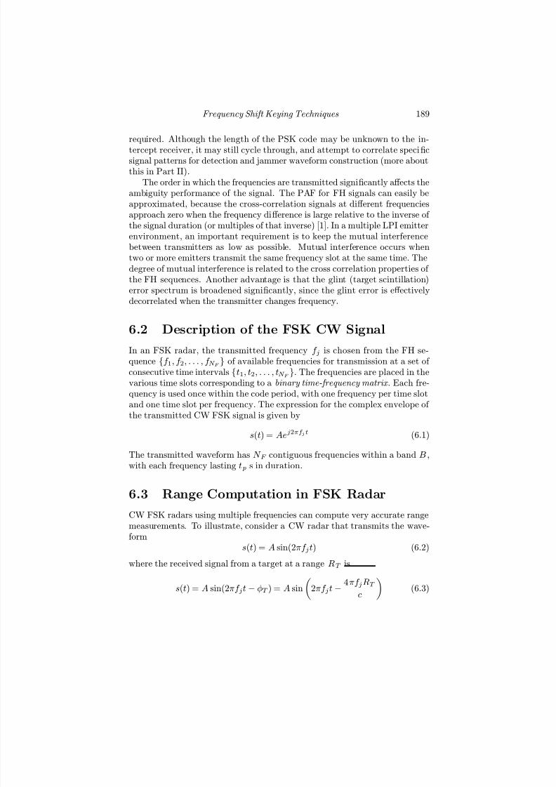
7/17/2019 1596932341 Intercept Radar.pdf
http://slidepdf.com/reader/full/1596932341-intercept-radarpdf 220/891
Frequency Shift Keying Techniques 189
required. Although the length of the PSK code may be unknown to the in-tercept receiver, it may still cycle through, and attempt to correlate specificsignal patterns for detection and jammer waveform construction (more aboutthis in Part II).
The order in which the frequencies are transmitted significantly aff ects theambiguity performance of the signal. The PAF for FH signals can easily beapproximated, because the cross-correlation signals at diff erent frequenciesapproach zero when the frequency diff erence is large relative to the inverse of the signal duration (or multiples of that inverse) [1]. In a multiple LPI emitterenvironment, an important requirement is to keep the mutual interferencebetween transmitters as low as possible. Mutual interference occurs whentwo or more emitters transmit the same frequency slot at the same time. Thedegree of mutual interference is related to the cross correlation properties of the FH sequences. Another advantage is that the glint (target scintillation)error spectrum is broadened significantly, since the glint error is eff ectivelydecorrelated when the transmitter changes frequency.
6.2 Description of the FSK CW Signal
In an FSK radar, the transmitted frequency f j is chosen from the FH se-quence f 1, f 2, . . . , f N F of available frequencies for transmission at a set of consecutive time intervals t1, t2, . . . , tN F . The frequencies are placed in thevarious time slots corresponding to a binary time-frequency matrix . Each fre-quency is used once within the code period, with one frequency per time slotand one time slot per frequency. The expression for the complex envelope of
the transmitted CW FSK signal is given by
s(t) = Aej2πf jt (6.1)
The transmitted waveform has N F contiguous frequencies within a band B ,with each frequency lasting t p s in duration.
6.3 Range Computation in FSK Radar
CW FSK radars using multiple frequencies can compute very accurate rangemeasurements. To illustrate, consider a CW radar that transmits the wave-form
s(t) = A sin(2πf jt) (6.2)where the received signal from a target at a range RT is
s(t) = A sin(2πf jt − φT ) = A sin
2πf jt −
4πf jRT
c
(6.3)

7/17/2019 1596932341 Intercept Radar.pdf
http://slidepdf.com/reader/full/1596932341-intercept-radarpdf 221/891
190 Detecting and Classifying LPI Radar
Solving for RT
RT = c
4πf jφT (6.4)
The unambiguous range occurs when φT is maximum or φT = 2π and there-fore with one frequency, RT is limited to extremely small values that are notpractical [3]. If two frequencies are used
s1(t) = A1 sin(2πf 1t) (6.5)
ands2(t) = A2 sin(2πf 2t) (6.6)
the received signals are
s1(t) = A1 sin(2πf 1t − φT 1) = A sin
2πf 1t −
4πf 1RT
c
(6.7)
and
s2(t) = A2 sin(2πf 2t − φT 2) = A sin
2πf 2t −
4πf 2RT
c
(6.8)
After mixing with the carrier frequency in the receiver, the phase diff erencebetween the two signals is
∆φT = 4πRT
c (f 2 − f 1) =
4πRT
c ∆f (6.9)
Since RT is maximum when ∆φ = 2π, the maximum unambiguous range is
Ru = c
2∆f (6.10)
and is very large since ∆f << c. From the measurement of the phase diff er-ence, ∆φT , the range of the target is then
RT = c∆φT
4π∆f (6.11)
This can also be written as a function of just the phase diff erence as
RT = Ru
∆φT
2π (6.12)
Since the range to the target depends on the frequency diff erence, therange resolution then depends on the duration of each frequency as
∆R = ct p
2 (6.13)

7/17/2019 1596932341 Intercept Radar.pdf
http://slidepdf.com/reader/full/1596932341-intercept-radarpdf 222/891
Frequency Shift Keying Techniques 191
The transmitted power for each frequency must be such that the energy con-tent within the target echo is sufficient for detection, and enough to ensurethat accurate phase measurements can be made.
In summary, for the FSK CW radar, the frequency di ff erence ∆f de-termines the maximum unambiguous detection range. The target’s range iscomputed by measuring the return signal phase diff erence from two consecu-tive transmitted frequencies. The range resolution, ∆R, depends only on theFH period.
6.4 Costas Codes
In a study by J. P. Costas, techniques were presented for generating a sequence
of frequencies that produce unambiguous range and Doppler measurementswhile minimizing the cross talk between frequencies [4]. In general, the Costassequence of frequencies provides an FH code that produces peak side lobesin the PAF, that are down from the main lobe response by a factor of 1 /N F for all regions in the delay-Doppler frequency plane. That is, the order of frequencies in a Costas sequence or array is chosen in a manner to preservean ambiguity response with a thumbtack nature (the narrow main lobe andside lobes are as low as possible). The firing order of these frequencies isbased on primitive roots (elements) of finite fields.
6.4.1 Characteristics of a Costas Array or Sequence
A Costas array or (frequency) sequence f 1, · · · , f N F is a sequence that is a
permutation of the integers 1, · · · , N F satisfying the property
f k+i − f k = f j+i − f j (6.14)
for every i, j, and k such that 1 ≤ k < i < i + j ≤ N F . An array thatresults from a Costas sequence in this way is called a Costas array [5]. Thenonequivalence condition in (6.14) can be checked easily when the frequencysequence is expressed in an N F − 1 × N F di ff erence triangle . As an addedbonus, the diff erence triangle can also be used to derive the PAF. We discusshow to derive Costas sequences in the next section and in Appendix C.
Consider the frequency sequence f j = 2, 4, 8, 5, 10, 9, 7, 3, 6, 1 kHz. Fig-ure 6.1(a) shows the binary time-frequency matrix for this sequence. Thefrequencies are fired at each ti and are indicated by a “1” in the matrix. The
power spectral density of the signal is shown in Figure 6.1(b). Also indicatedis the firing order for each frequency. If the subperiod t p (frequency duration)is constant, the cycle density or number of cycles per frequency varies as t pf j .
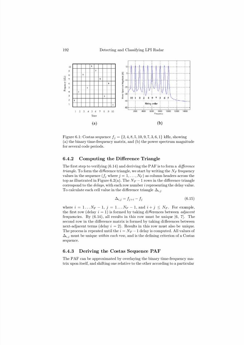
7/17/2019 1596932341 Intercept Radar.pdf
http://slidepdf.com/reader/full/1596932341-intercept-radarpdf 223/891
192 Detecting and Classifying LPI Radar
Figure 6.1: Costas sequence f j = 2, 4, 8, 5, 10, 9, 7, 3, 6, 1 kHz, showing(a) the binary time-frequency matrix, and (b) the power spectrum magnitudefor several code periods.
6.4.2 Computing the Diff erence Triangle
The first step to verifying (6.14) and deriving the PAF is to form a di ff erence
triangle . To form the diff erence triangle, we start by writing the N F frequencyvalues in the sequence (f j where j = 1, . . . , N F ) as column headers across the
top as illustrated in Figure 6.2(a). The N F −1 rows in the diff erence trianglecorrespond to the delays , with each row number i representing the delay value.To calculate each cell value in the diff erence triangle ∆i,j
∆i,j = f j+i − f j (6.15)
where i = 1 . . . N F − 1, j = 1 . . . N F − 1, and i + j ≤ N F . For example,the first row (delay i = 1) is formed by taking diff erences between adjacent
frequencies. By (6.14), all results in this row must be unique [6, 7]. Thesecond row in the diff erence matrix is formed by taking diff erences betweennext-adjacent terms (delay i = 2). Results in this row must also be unique.The process is repeated until the i = N F −1 delay is computed. All values of ∆i,j must be unique within each row , and is the defining criterion of a Costas
sequence.
6.4.3 Deriving the Costas Sequence PAF
The PAF can be approximated by overlaying the binary time-frequency ma-trix upon itself, and shifting one relative to the other according to a particular

7/17/2019 1596932341 Intercept Radar.pdf
http://slidepdf.com/reader/full/1596932341-intercept-radarpdf 224/891
Frequency Shift Keying Techniques 193
delay (horizontal shifts) and particular Doppler (vertical shifts). At each com-bination of shifts, the sum of coincidences between points of the fixed andthe shifted matrix, represents the relative height of the PAF. An easier wayto derive the PAF is using the diff erence triangle, as shown in Figure 6.2(a).In Figure 6.2(b) the PAF of the 10-frequency Costas signal is derived fromthe diff erence triangle. The PAF is constructed by considering each row (de-lay) in the diff erence triangle, and placing a “1” in the PAF delay-Dopplercell corresponding to each ∆i,j. The delay i = 1 is shaded as an exam-ple. The PAF derived from this complex Costas signal with f s = 27.5 kHz(power spectrum magnitude shown in Figure 6.1) is shown for comparison inFigure 6.2(c).
6.4.4 Welch Construction of Costas ArraysThere are many analytical procedures for constructing Costas frequency hop-ping arrays. Although Costas arrays may exist in principle for any positiveinteger N F , these analytical construction methods are typically limited tovalues of N F related to prime numbers [6, 8, 9]. Most construction methodsto produce a large number of Costas arrays of equal length are based on theproperties of primitive roots (see the tutorial in Appendix C).
For the Welch construction of a Costas array, an odd prime number p ischosen first. The number of frequencies and the number of time slots in theCostas sequence are then N F = φ( p) = p−1 where φ( p) is the Euler function.Next, a primitive root g modulo p is chosen. As discussed in Appendix C, if gis a primitive root modulo p, then g is an integer belonging to the Euler-φ( p)function modulo p. Since g is a primitive root modulo p, g , g2, . . . , gφ( p) aremutually incongruent and form a permuted sequence of the reduced residues
p. Welch showed that this reduced residue sequence is a Costas sequence.
Theorem 6.1 Let g be a primitive root of an odd prime number p. Then the( p−1) by ( p−1) permutation matrix A has elements ai,j =1 iff j ≡ gi(mod p)for 1 ≤ i, j ≤ p− 1 and this is a Costas array [10].
Example: The first step is choosing a prime number p. We choose the primenumber p = 7. For p = 7, N F = 6, which is the number of frequenciesin the FH code. The complete residue system is 0, 1, 2, 3, 4, 5, 6. With pprime, we know that the number of elements in the reduced residue systemis φ( p) = p − 1 = 6. The reduced residue system is 1, 2, 3, 4, 5, 6 (deleting
the one element that is divisible by p). From Appendix C, for p = 7 we knowthere are exactly φφ(7) = φ6 = 2 mutually incongruent primitive rootsmodulo p = 7. We start with the smallest value g = 2, but the order of g =2is 3 (not 6). Next we pick g = 3 and get the desired result 3, 2, 6, 4, 5, 1,which is the Costas array as shown below. The left-hand column shows ifrom 1 to p − 1, and the right-hand column shows the frequency j using

7/17/2019 1596932341 Intercept Radar.pdf
http://slidepdf.com/reader/full/1596932341-intercept-radarpdf 225/891
194 Detecting and Classifying LPI Radar
Figure 6.2: Costas sequence with (a) the diff erence triangle, (b) the PAFderived from the diff erence triangle, and (c) the PAF derived from the complexsignal.

7/17/2019 1596932341 Intercept Radar.pdf
http://slidepdf.com/reader/full/1596932341-intercept-radarpdf 226/891
Frequency Shift Keying Techniques 195
Theorem 6.1.
i j = gi(mod7)1 31 = 32 32 = 23 33 = 64 34 = 45 35 = 56 3 p−1 = 36 = 1
where i, j = 1, 2, . . . , 6. Consequently, the Costas frequency sequence is
f = 3, 2, 6, 4, 5, 1 (6.16)
Note from the symmetry that f = 5, 4, 6, 2, 3, 1 is also a Costas sequence.The Welch construction is also singly periodic [5]. That is, the sequence
f i, f i+1, . . . , f i+ p−2 is also a Costas sequence. Any circular shift of the se-quence is also a Costas sequence. The costas.m program within the LPITallows the user to quickly add additional sequences that may be of interest.
6.5 Hybrid FSK/PSK Technique
The hybrid LPI radar technique discussed in this section combines the tech-nique of FSK (FH using Costas sequences) with that of a PSK modulation
using sequences of varying length [11, 12]. This type of signaling can achieve ahigh time-bandwidth product or processing gain, enhancing the LPI featuresof the radar. Ambiguity properties of the signal are retained by preservingthe desirable properties of the separate FSK and PSK signaling schemes. TheFSK/PSK techniques can maintain a high Doppler tolerance, while yieldingan instantaneous spreading of the component frequencies along with an en-hanced range resolution [11]. Below, a Costas-based FSK/PSK signal (Barker5-bit PSK over each frequency) is investigated as an example. Other PSKtechniques from Chapter 5 can also be investigated using the LPIT.
6.5.1 Description of the FSK/PSK Signal
Recall that for the FH LPI radar, the CW waveform has N F contiguous fre-
quencies within a bandwidth B , with each frequency lasting t p s in duration.The hybrid FSK/PSK signal further subdivides each subperiod into N B phaseslots, each of duration tb as shown in Figure 6.3. The total number of phaseslots in the FSK/PSK waveform is then
N T = N F N B (6.17)

7/17/2019 1596932341 Intercept Radar.pdf
http://slidepdf.com/reader/full/1596932341-intercept-radarpdf 227/891
196 Detecting and Classifying LPI Radar
Figure 6.3: General FSK/PSK signal containing N F frequency subcodes(hops) each with duration t p s. Each frequency subcode is subdivided into
N B phase slots, each with duration tb.
with the total code period T = tbN BN F . The expression for the complexenvelope of the transmitted CW FSK/PSK signal is given by
s(t) = Aej2πf jt+φk (6.18)
where φk is one of N B Barker codes for this example, and f j is one of N F Costas frequencies.
During each hop, the signal frequency (one of N F frequencies) is modu-lated by a binary phase sequence, according to a Barker sequence of lengthN B = 5, 7, 11, or 13. As an example, the FSK/PSK signal generated byusing the N F = 6 Costas sequence (6.16), and phase modulating it with a
Barker binary phase modulation of length N B = 5 gives the signal: S = 3
+
,3+, 3+, 3−, 3+, 2+, 2+, 2+, 2−, 2+, 6+, 6+, 6+, 6+, 6−, 4+, 4+, 4+, 4−,4+, 5+, 5+, 5+, 5−, 5+, 1+, 1+, 1+, 1−, 1+. The final waveform is a binaryphase modulation within each frequency hop, resulting in five phase subcodesequally distributed within each frequency, for a total of N P N F =30 subcodes.
Figure 6.4 shows the power spectrum magnitude that reveals the spreadspectrum characteristic of the phase-modulated Costas signalf = 3, 2, 6, 4, 5, 1 kHz. For this signal, the sampling frequency f s = 15kHz, the subperiod for each frequency is t p =6 ms (B = 167 Hz) and anN B = 5-bit Barker code is used. Figure 6.4(a) shows the Costas sequencepower spectrum magnitude before phase modulation. Figure 6.4(b) showsthe power spectrum magnitude of the Costas sequence FSK/PSK after phasemodulation. Figure 6.5(a, b) shows the ACF and the PACF, respectively, of
the FSK/PSK sequence. Note the phase modulation spikes that are presentwith regular periodicity. Figure 6.6 shows the PAF and the Doppler sidelobes present. The fsk psk costas.m program within the LPIT allows addi-tional phase modulations to be included with the Costas sequences (which canalso be easily changed). In this manner, the side lobe structure for variousphase modulations can be easily compared.

7/17/2019 1596932341 Intercept Radar.pdf
http://slidepdf.com/reader/full/1596932341-intercept-radarpdf 228/891
Frequency Shift Keying Techniques 197
Figure 6.4: Power spectrum magnitude plot for a Costas waveform, with(a) no phase modulation and (b) 5-bit phase modulation.

7/17/2019 1596932341 Intercept Radar.pdf
http://slidepdf.com/reader/full/1596932341-intercept-radarpdf 229/891
198 Detecting and Classifying LPI Radar
Figure 6.5: (a) ACF and (b) PACF plot for the Costas sequence with a 5-bitBarker phase modulation.
Figure 6.6: PAF plot for the Costas sequence with a 5-bit Barker phasemodulation.
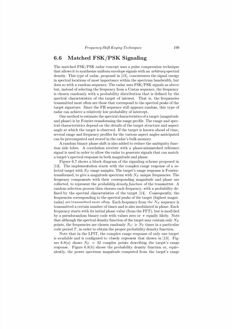
7/17/2019 1596932341 Intercept Radar.pdf
http://slidepdf.com/reader/full/1596932341-intercept-radarpdf 230/891
Frequency Shift Keying Techniques 199
6.6 Matched FSK/PSK SignalingThe matched FSK/PSK radar concept uses a pulse compression techniquethat allows it to synthesize uniform envelope signals with an arbitrary spectraldensity. This type of radar, proposed in [13], concentrates the signal energyin spectral locations of most importance within the spectrum bandwidth, butdoes so with a random sequence. The radar uses FSK/PSK signals as abovebut, instead of selecting the frequency from a Costas sequence, the frequencyis chosen randomly with a probability distribution that is defined by thespectral characteristics of the target of interest. That is, the frequenciestransmitted most often are those that correspond to the spectral peaks of thetarget signature. Since the FH sequence still appears random, this type of radar can achieve a relatively low probability of intercept.
One method to estimate the spectral characteristics of a target (magnitudeand phase) is by Fourier-transforming the range profile. The range and spec-tral characteristics depend on the details of the target structure and aspectangle at which the target is observed. If the target is known ahead of time,several range and frequency profiles for the various aspect angles anticipatedcan be precomputed and stored in the radar’s bulk memory.
A random binary phase shift is also added to reduce the ambiguity func-tion side lobes. A correlation receiver with a phase-mismatched referencesignal is used in order to allow the radar to generate signals that can matcha target’s spectral response in both magnitude and phase.
Figure 6.7 shows a block diagram of the signaling scheme proposed in[13]. The implementation starts with the complex range response of a se-lected target with N F range samples. The target’s range response is Fourier-transformed, to give a magnitude spectrum with N F unique frequencies. Thefrequency components with their corresponding magnitude and phase arecollected, to represent the probability density function of the transmitter. Arandom selection process then chooses each frequency, with a probability de-fined by the spectral characteristics of the target [14]. Consequently, thefrequencies corresponding to the spectral peaks of the target (highest magni-tudes) are transmitted more often. Each frequency from the N F sequence istransmitted a certain number of times and is also modulated in phase. Eachfrequency starts with its initial phase value (from the FFT), but is modi fiedby a pseudorandom binary code with values zero or π equally likely. Notethat although the spectral density function of the target may contain only N F points, the frequencies are chosen randomly N C N T times in a particular
code period T , in order to obtain the proper probability density function.Note that in the LPIT, the complex range response of only one targetis available and is configured to closely represent that shown in [13]. Fig-ure 6.8(a) shows N F = 32 complex points describing the target’s rangeresponse. Figure 6.8(b) shows the probability density function or, equiv-alently, the power spectrum magnitude computed from the target’s range

7/17/2019 1596932341 Intercept Radar.pdf
http://slidepdf.com/reader/full/1596932341-intercept-radarpdf 231/891
200 Detecting and Classifying LPI Radar
Figure 6.7: Block diagram of the generation of an FSK/PSK target matchedwaveform.

7/17/2019 1596932341 Intercept Radar.pdf
http://slidepdf.com/reader/full/1596932341-intercept-radarpdf 232/891
Frequency Shift Keying Techniques 201
response. The histogram of the transmitted frequency hopping signal isshown in Figure 6.9(a). This figure shows how many times each one of N F =32 frequencies is transmitted in the N C =512 frequency code. Note the similarappearance to the probability density function shown inFigure 6.9(b), and the power spectrum magnitude given in Figure 6.8(b).Increasing the number of random frequency selections N C > 512, will resultin an even better match. Figure 6.10 shows the resulting power spectrummagnitude for the transmitted signal, revealing the wideband nature of thistype of hybrid FSK/PSK signaling. Figure 6.11(a) shows the ACF of thetransmitted waveform. Note the near-uniform side lobes that are down closeto −30 dB. The PACF is shown in Figure 6.11(b), and shows the absenceof any periodic components. The PAF shown in Figure 6.12 shows a spikeat (τ /tb = 0, ν ∗ N ctb = 0) and very low side lobes, resembling the PAF of random noise.
6.7 Concluding Remarks
FSK signals provide a higher probability of detection compared to PSK andFMCW signals, but off er many advantages for LPI signaling. Combined withPSK, significant LPI results can be obtained. The FSK, FSK/PSK pulsecompression signals discussed in this chapter can help a radar achieve LPIgoals. The waveforms can be generated using the LPI toolbox main menuprogram lpit.m contained on the MATLAB CD.
The hybrid modulations presented in this chapter tend to make the trans-mitted signal appear as noise-enhancing its low probability of intercept na-
ture. These hybrid techniques are a subset of a larger group of radar architec-tures known as random signal or noise radar. Random signal radar techniquescan derive target detections using correlation, spectrum analysis, or anticor-relation. Random signal radar modulations include: noise FMCW, sine plusnoise FMCW, random binary PSK CW, and random pulse modulation [15].Because of the random nature of the transmitted waveform, random signalradar also provides a good deal of electronic protection and has a counter-electronic support capability [16]. These techniques are examined in detail inthe next chapter.

7/17/2019 1596932341 Intercept Radar.pdf
http://slidepdf.com/reader/full/1596932341-intercept-radarpdf 233/891
202 Detecting and Classifying LPI Radar
Figure 6.8: Transmitted signal showing (a) 32 complex points describing thesimulated range response and (b) the normalized power spectrum magnituderepresenting the probability density function. (After [13].)
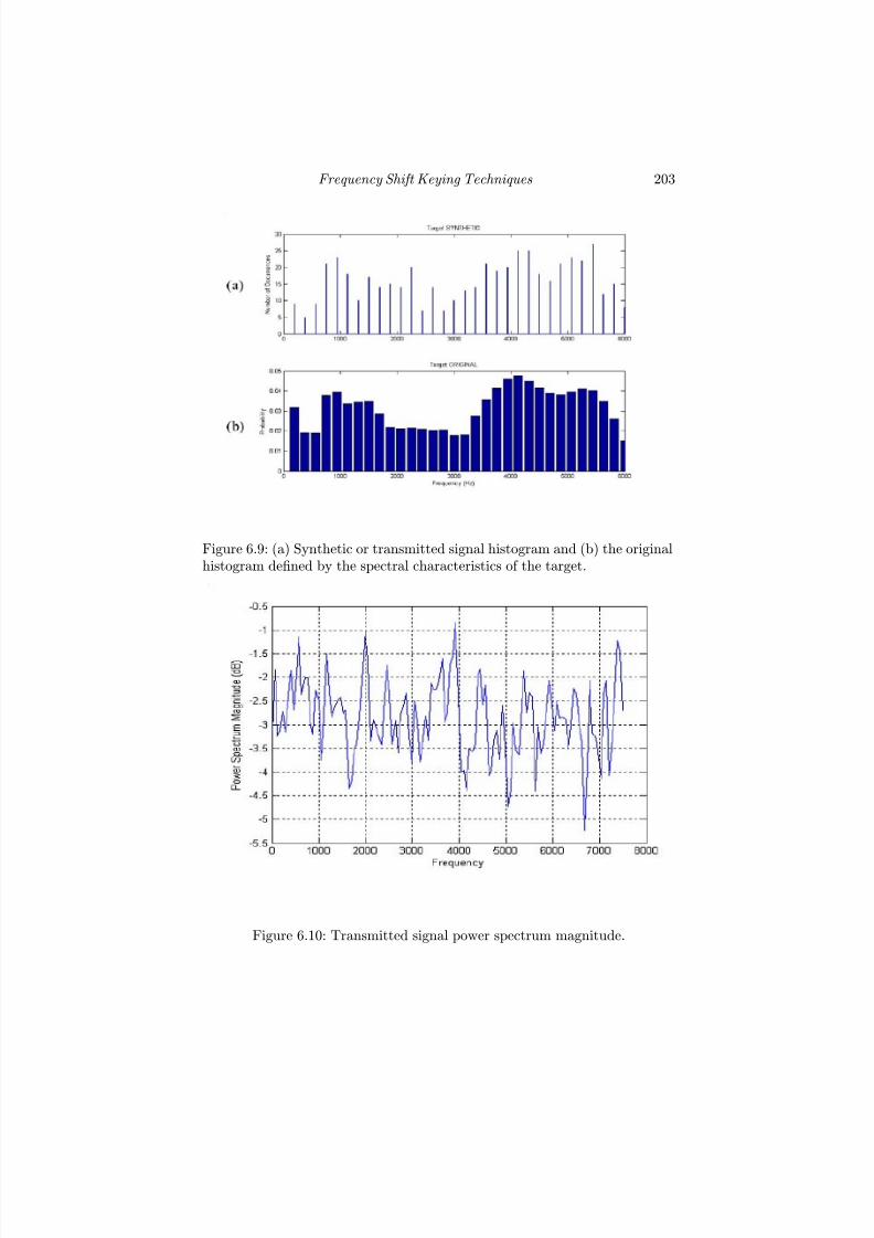
7/17/2019 1596932341 Intercept Radar.pdf
http://slidepdf.com/reader/full/1596932341-intercept-radarpdf 234/891
Frequency Shift Keying Techniques 203
Figure 6.9: (a) Synthetic or transmitted signal histogram and (b) the originalhistogram defined by the spectral characteristics of the target.
Figure 6.10: Transmitted signal power spectrum magnitude.
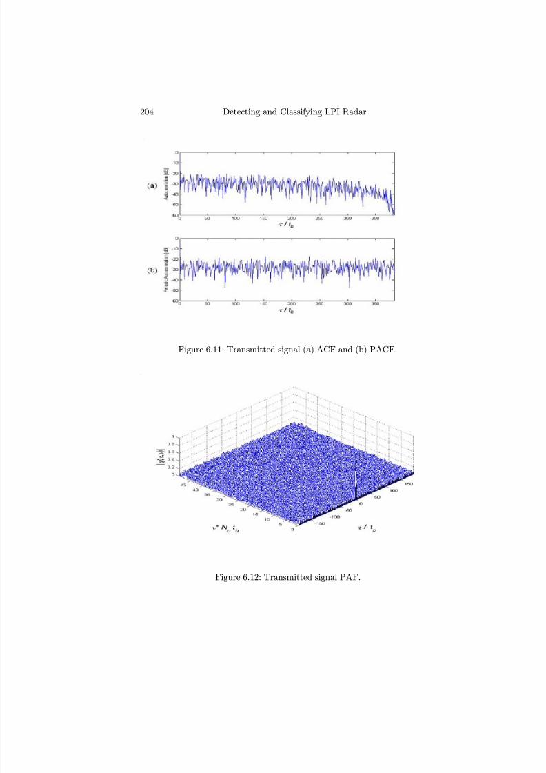
7/17/2019 1596932341 Intercept Radar.pdf
http://slidepdf.com/reader/full/1596932341-intercept-radarpdf 235/891
204 Detecting and Classifying LPI Radar
Figure 6.11: Transmitted signal (a) ACF and (b) PACF.
Figure 6.12: Transmitted signal PAF.

7/17/2019 1596932341 Intercept Radar.pdf
http://slidepdf.com/reader/full/1596932341-intercept-radarpdf 236/891
Frequency Shift Keying Techniques 205
References[1] Sanmartin-Jara, J., Burgos-Garcia, M., and Retamosa-Sanchez, J., “Radar
sensor using low probability of interception SS-FH signals,” IEEE Aerospace
and Electronics Magazine, pp. 23—28, April 2000.
[2] Benn, H. P. and Jones, W. J., “A fast hopping frequency synthesizer,” Second
International Conference on Frequency Control and Synthesis , pp. 69—72,April 1989.
[3] Mahafza, B. R., Radar Systems Analysis and Design Using MATLAB, Chap-man & Hall/CRC, New York, 2000.
[4] Costas, J. P., “A study of a class of detection waveforms having nearly idealrange-Doppler ambiguity properties,” Proc. of the IEEE, Vol. 72, No. 8, pp.996—1009, August 1984.
[5] Golomb, S. W., and Moreno, O., “On periodicity properties of Costas arraysand a conjecture on permutation polynomials,” IEEE Trans. on Information
Theory, Vol. 42, No. 6, pp. 2252—2253, Nov. 1996.
[6] Golomb, S. W., and Taylor, H., “Construction and properties of Costas ar-rays,” Proc. of the IEEE, Vol. 72, No. 9, pp. 1143—1163, Sept. 1984.
[7] Levanon, N., Radar Principles, John Wiley & Sons, New York, NY 1988.
[8] Maric, S. V., Seskar, I., and Titlebaum, E. L., “On cross-ambiguity propertiesof Welch-Costas arrays,” IEEE Trans. on Aerospace and Electronic Systems,
Vol. 30, No. 4, pp. 1063—1071, Oct. 1994.
[9] O’Carroll, L., et al., “A study of auto- and cross-ambiguity surface per-formance for discretely coded waveforms,” IEE Proc. F Radar and Signal
Processing, Vol. 137, No. 5, pp. 362—370, Oct. 1990.
[10] Lemieux, J. A., “Analysis of an optimum hybrid radar waveform using fre-quency hopping and locally optimum signals,” Proc. of the IEEE National
Radar Conference, pp. 98—102, March 12—13, 1991.
[11] Donohoe, J. P., and Ingels, F. M., “The ambiguity properties of FSK/PSKsignals,” Record of the IEEE 1990 International Radar Conference, 1990, pp.268—273 May 7—10, 1990.
[12] Skinner, B. J., Donohoe, J. P., and Ingels, F. M., “Simplified performanceestimation of FSK/PSK hybrid signaling radar systems,” Proc. of the IEEE
1993 National Aerospace and Electronics Conference, NAECON, Vol. 1, pp.255—261, May 24—28, 1993.
[13] Skinner, B. J., Donohoe, J. P., and Ingels, F. M., “Matched FSK/PSK radar,”Record of the 1994 IEEE National Radar Conference, pp. 251—255, March29—31, 1994.
[14] Marsaglia, G., “Random variables and computers,” Proc. of the Third Prague Conference on Information Theory, Statistical Decision Functions, Random
Processes, Liblice, pp. 499—512, June 5—13, 1962.
[15] Guosui, L., Hong, G., and Weimin, S., “Development of random signal radars,”IEEE Trans. on Aerospace and Electronic Systems, Vol. 35, No. 3, pp. 770—777, July 1999.

7/17/2019 1596932341 Intercept Radar.pdf
http://slidepdf.com/reader/full/1596932341-intercept-radarpdf 237/891
206 Detecting and Classifying LPI Radar
[16] Garmatuk, D. S., and Narayanan, R. M., “ECCM capabilities of an ultrawide-band bandlimited random noise imaging radar,” IEEE Trans. on Aerospace
and Electronic Systems, Vol. 38, No. 4, pp. 1243—1255, Oct. 2002.
Problems
1. An FSK CW radar is required to perform ranging up to a maximum of 15 nmi. What is the required frequency diff erence ∆f ?
2. Derive the Costas frequency sequence given in Figure 6.1. Hint: Startby choosing the correct prime modulus p and writing down the twoprimitive roots.
3. The frequency hopping sequence
3, 9, 10, 13, 5, 15, 11, 16, 14, 8, 7, 4, 12, 2, 6, 1
is being considered for a new LPI radar. (a) Show that this is a Costassequence. (b) If so, how many primitive roots are there? (c) Derive thesequence by determining p and the primitive roots.
4. Consider the Welch construction of a Costas frequency hopping se-quence with p = 13. (a) How many frequencies are contained in thefrequency hopping sequence? (b) Write the elements of the reduced
residue system. (c) How many primitive roots are there in the system?Do not forget to show your work. (d) What are the primitive roots of
the system? (e) Write out the Costas sequence for each primitive root.(f) For the sequence resulting from the largest primitive root, show thatthe sequence is Costas by forming the diff erence triangle. (g) Draw acontour grid of the periodic ambiguity function for the sequence in (f)making sure that you label the side lobe levels and main peak amplitude.
5. (a) Edit the costas.m file to include the Costas sequence given in (6.16).(b) Compute the power spectrum magnitude and PAF of this sequence.
6. Using the fsk psk costas.m file, generate the power spectrum, ACF,PACF, and PAF for the first Costas sequence with (a) N B = 5 and(b) N B = 13. What is the diff erence in the side lobe level you observe?
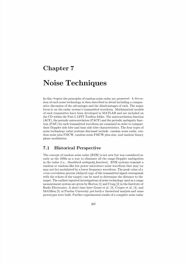
7/17/2019 1596932341 Intercept Radar.pdf
http://slidepdf.com/reader/full/1596932341-intercept-radarpdf 238/891
Chapter 7
Noise Techniques
In this chapter the principles of random noise radar are presented. A discus-sion of each noise technology is then described in detail including a compar-ative discussion of the advantages and the disadvantages of each. The majorfocus is on the radar system’s transmitted waveform. Mathematical modelsof each transmitter have been developed in MATLAB and are included onthe CD within the Part I, LPIT Toolbox folder. The autocorrelation function(ACF), the periodic autocorrelation (PACF) and the periodic ambiguity func-tion (PAF) for each transmitted waveform are examined in order to comparetheir Doppler side lobe and time side lobe characteristics. The four types of noise technology radar systems discussed include: random noise radar, ran-dom noise plus FMCW, random noise FMCW plus sine, and random binary
phase modulation.
7.1 Historical Perspective
The concept of random noise radar (RNR) is not new but was considered asearly as the 1950s as a way to eliminate all the range-Doppler ambiguitiesin the radar (i.e., thumbtack ambiguity function ). RNR systems transmit arandom or random-like low power microwave noise waveform that may (ormay not be) modulated by a lower frequency waveform. The peak value of across-correlation process (delayed copy of the transmitted signal correspondswith the echoes of the target) can be used to determine the distance to thetarget. The earliest reported investigations of noise technology used as a range
measurement system are given by Horton [1] and Craig [2] in the Institute of Radio Electronics. A short time later Grant et al. [3], Cooper et al. [4], andMcGillem [5] at Purdue University put forth a theoretical analysis and someprototypes were built. Further experimental results of a complete noise radar
207
7/17/2019 1596932341 Intercept Radar.pdf
http://slidepdf.com/reader/full/1596932341-intercept-radarpdf 239/891
208 Detecting and Classifying LPI Radar
system were obtained in [6] showing that it was possible to detect a target invery poor SNR conditions even with nonoptimum hardware.
The research however, was quickly dropped since the development of noisewaveform sources with the required bandwidth was difficult. Also since cross-correlation processing of the transmitted and received signal was necessarythe use of variable microwave delay lines was required [7]. Before the 1960s,the manufacturing of these devices was complicated. From the 1960s to the1970s, the research into RNR ramped up quickly and several experimentalsystems were built and tested. A good overview of the diff erent techniques isgiven in [8] and an extensive bibliography of the early development in RNRis given in [9].
With the development of solid-state microwave techniques and high-speedintegrated VLSI circuits the technology began to support the RNR conceptsand implement the required processing. Today the RNR waveform can be gen-erated digitally followed by a digital-to-analog converter and up-conversiononto a carrier signal. They are also relatively inexpensive to build and manydiff erent variants on the RNR are possible including the use of UWB wave-forms.
Noise technology radar can be used to detect targets in both range andDoppler. RNR emitters have good electronic protection properties by pos-sessing a natural immunity to jamming and interference from other radarsystems operating in the same theater of operations [10, 11]. The use of aRNR provides the advantage that it is uncorrelated with the intentional andunintentional interference as well as other noise sources. That is, the correla-tion process used in the receiver allows it to sort out the incoming signals even
within the same band making it attractive in multi radar environments [10].These advantages are due to the properties of the RNR featureless waveform .These include transmitting the lowest obtainable instantaneous power spec-tral density possible by spreading its energy over a wide signal bandwidth andthe use of non-redundant waveforms that appear random and are concealedin the ambient thermal noise and interference environment [12].
The exception is the use of deception . Deception is a repeater technique(constant gain) in which false targets are created in the radar receiver thatare interpreted as valid targets. The jam-to-signal ratio is independent of therange between the repeater jammer and the radar. Post detection integrationof target signal returns can normally provide a significant decrease in jam-to-signal ratio however, for deception techniques, the integration gain is equalfor valid and false targets.
RNR systems that use random noise also have a significant processinggain unavailable to the noncooperative intercept receiver since their low meanpower and noise-like characteristics result in a very low SNR. Even if thesignal is detected, it is unlikely to be identified making these types of emittersimportant for many LPI and LPID applications.
RNR systems and waveforms are becoming useful in certain (limited) ap-

7/17/2019 1596932341 Intercept Radar.pdf
http://slidepdf.com/reader/full/1596932341-intercept-radarpdf 240/891
Noise Techniques 209
plications such as acoustic radar—usually called sodar (sound detection andranging) [13]. Also of growing importance are the high-resolution measure-ment of range profiles for foliage- and ground-penetrating detection of buriedobjects such as mines [14—17], inverse synthetic aperture radar (ISAR) andsynthetic aperture (SAR) imaging [18, 19]. Covert tracking of targets usingRNR monopulse techniques are discussed in [20—22]. Car collision warningand avoidance systems and UAV landing systems are also being investigated[7]. The detection of small-RCS targets in surface clutter depends on thesignal-to-clutter ratio (SCR) in the target range resolution cell and the abil-ity to resolve the target signal in Doppler. The SCR (in the absence of rangeambiguity) is the ratio of target RCS to clutter RCS, and for diff erent wave-forms the clutter RCS depends on the signal bandwidth and the possiblepresence of range side lobes. Surface clutter (especially at low grazing an-gles) is notably spiky, with peaks having dimensions on the order of 1m, soa range resolution cell smaller than the target length is of limited value intarget detection.
There are many waveform options that can be matched to the radial di-mension of a small-RCS target, or to the dimension of dominant scattererswithin the target and noise waveforms have no unique advantage in this re-spect. For the noise waveforms, the range cells are formed by stepwise delay of the transmitted reference signal however, the use of a nonperiodic waveformsuppresses the range ambiguity. The Doppler cells are created by step-wisevarying the time compression of the reference signal at the correlation oper-ation. The Doppler resolution depends on the coherent processing intervaland is limited by the same factors for all waveform types and therefore noise
waveforms do not have any particular advantage here as well. Due to therandomness of the waveform, a noise floor is present in the correlation in-tegral that limits the possible side lobe suppression. In strong clutter, theintegrated side lobe contribution can be very large and clutter cancelationmethods are required.
Recently, there has been much interest in multiple-input multiple-output(MIMO) radar systems. MIMO techniques have been well studied in commu-nications off ering advantages where multipath environments can cause fading.Radar waveform rejection of multipath requires that the range resolution cellbe smaller than the range diff erence δ between the direct and multipath echoes(even if range side lobes are absent). The range diff erence between the directpath and the multipath echoes can be expressed as
δ ≈2hrht
R
where hr and ht are the radar and target altitudes and R is the range. For alow-grazing-angle target not resolvable by the antenna beamwidth, the rangediff erence can be quite small. Even if the waveform bandwidth were increasedto make the resolution smaller than this range diff erence, the scatterers in

7/17/2019 1596932341 Intercept Radar.pdf
http://slidepdf.com/reader/full/1596932341-intercept-radarpdf 241/891
210 Detecting and Classifying LPI Radar
the initial range cell of the target would have to be large enough to providea signal for tracking, before the multipath catches up with the direct signaland generates a tracking error. Whether a noise waveform or other type of waveform is used, resolution of this sort has not provided significant trackingadvantages in any known system.
The majority of MIMO radar configurations have focused on multistaticarrays that have sufficient spatial separation to decorrelate the target’s radarcross section scintillation. These networks combine the received data non-coherently to average out the scintillations. Another form of MIMO radaruses multiple orthogonally coded waveforms from individual transmitter ele-ments of a phased array which are then combined coherently upon receive toform multiple beams [23]. Recently, the extension of noise radar to MIMOconfigurations has been explored. Two transmission techniques are describedand include an element-space and beam-space approach [24]. In the element-space approach, K channels of independent (noncoherent) noise are transmit-ted separately by K omnidirectional antennas. In the beam-space approach,each independent noise source is fed into each antenna but is either delayed orphase shifted so as to form a beam illuminating a selected sector of the radarsystem’s field of view-eff ectively coding each sector according to a particularnoise source. The direction of each noise sector is determined by the phaseshifts and the sector width is determined by the beamwidth of the array.
7.2 Ultrawideband Considerations
The combination of RNR and ultrawideband (UWB) technology can give sig-
nificant benefits and overcome inherent drawbacks of narrowband radar. Afew definitions concerning UWB waveforms are given below. Consider for ex-ample a wideband RNR signal with bandwidth spanning f min to f max. Thefirst definition is for the absolute bandwidth B ,
Definition 7.1
The absolute bandwidth B defines the width of the frequencyinterval occupied by the signal’s spectrum and is the diff erencebetween the maximum frequency and the minimum frequency or
B = f max − f min (7.1)
The term ultrawideband (UWB) refers to waveforms that have aninstantaneous fractional bandwidth greater than 0.25 (25%) withrespect to the center frequency.

7/17/2019 1596932341 Intercept Radar.pdf
http://slidepdf.com/reader/full/1596932341-intercept-radarpdf 242/891
Noise Techniques 211
Definition 7.2
The instantaneous fractional bandwidth ∆f is defined as the ratioof the absolute bandwidth (f max − f min) to the mean frequency(f min + f max)/2. Thus the fractional bandwidth is defined as [25]
∆f =
2(f max − f min)
f min + f max
100% =
100%
0.5 + f min/B (7.2)
The maximum fractional bandwidth is 200% and is reached if f min = 0. Notethat this value is not f max dependent. A small fractional bandwidth ∆f indi-cates that the behavior of the radar system devices being used are not likely to
change much within the absolute bandwidth B . With a large ∆f , the devicebehavior may show changes throughout B because the device characteristicsmay be diff erent across the large number of transmit frequencies. That is,it is more difficult to build devices which cover a large bandwidth with thesame efficiency or properties.
Another important term used to evaluate UWB RNR signal bandwidthwhen the waveform is produced by random binary phase shifts is the spread-ing ratio (or processing gain) [26].
Definition 7.3
The spreading ratio or processing gain of a random binary phase
shift keying signal is defined as
P GR = T
tb= N c (7.3)
where T is the code period, tb is the subcode period and N c is thenumber of subcodes within a period.
The motivation to use UWB random noise emitters comes from the needto have fine range resolution and range measurement accuracy. In contrastto conventional narrowband systems, the UWB radar obtains much moreinformation about the material properties and the structure of scanned tar-gets. In the case of high SNR and precise calibration, range accuracy may
even approach millimeter wave (mm) and submillimeter levels. It also hasan enhanced clutter suppression capability which could someday lead to asolution for the difficult task of detecting a sea-skimming antiship capablemissile. Foliage-, wall- and ground- penetrating detection and imaging alsobenefit. For through-the-wall UWB radar, 1.99 GHz—10.6 GHz are allowed in

7/17/2019 1596932341 Intercept Radar.pdf
http://slidepdf.com/reader/full/1596932341-intercept-radarpdf 243/891
212 Detecting and Classifying LPI Radar
the United States (FCC) and 30 MHz—18 GHz frequency range is envisionedfor wall and ground penetrating radar in Europe [25].
An important aspect of the UWB radar in addition to its LPI and LPIDcharacteristics are its immunity from electromagnetic radiation eff ects whichenable frequency spectrum sharing and a significant immunity from deceptive
jamming. Note that noise jamming has the same eff ect on radar systems thatuse noise waveforms as it does on systems that use of any other type of waveforms of similar bandwidth. On the other hand, there are worries in thecommunity about the influence of the UWB RNR on small signal receiverdevices such as GPS, cell phone and wireless LAN communications [27].
Another major problem in the radar application of UWB noise waveformsis that they exhibit the “thumbtack” ambiguity function and require the useof a correlator that covers many range-Doppler cells to detect targets whoserange and velocity are unknown. The techniques examined in this chap-ter describe systems in which the correlator covers a single cell , requiringtwo-dimensional sequential search to detect targets with unknown position.Although useful for some geophysical applications, the technology is currentlyinadequate for most military radar applications. Detection of buried minesand tracking a target after it has been detected by other conventional wave-forms are examples of current military applications. The processing through-put for parallel coverage of large regions in range-velocity space is a majorproblem that must still be addressed.
7.3 Principles of Random Noise Radars
The ability to simultaneously measure range and Doppler is important fortarget detection and imaging and requires that the radar be phase coherent
[28]. This simultaneous measurement would be especially advantageous if itwere implemented in a real-time range-Doppler processor covering a usefulfield in both coordinates. Today no noise radars have this capability, and thisabsence currently constitutes a major disadvantage being addressed.
Although RNR is by definition, totally incoherent, it is possible to injectphase coherence into the radar using the technique of heterodyne correlation.Figure 7.1 shows the main components of a RNR system. A microwave CWnoise signal S (t) is transmitted, and the return signal from the target’s re-flectivity, delayed by td, is received and coherently detected. A copy of thetransmitted noise, delayed by T r (RF delay line), is used as a reference sig-nal that is cross-correlated with the received signal. The amount of delay of the reference signal is a measure of the target’s distance. The down rangeperformance of a random noise radar depends mainly on the cross-correlationfunction in the radar receiver. When T r is varied, a strong correlation peakis obtained for T r = td, which gives an estimate of the target’s range asR = ctd/2. Doppler processing can also be performed and the output of the

7/17/2019 1596932341 Intercept Radar.pdf
http://slidepdf.com/reader/full/1596932341-intercept-radarpdf 244/891
Noise Techniques 213
Figure 7.1: Main components of a noise radar using a delay line. (After [28].)
Doppler filters following the correlator can be used to calculate the velocityof the target.
Consider the detection of a point target. Following the development byAxelsson, the transmitted noise signal can be modeled as a stationary process
in complex form as [29, 30]
S (t) = [X (t) + jY (t)]exp( j2πf ct) (7.4)
where 2πf c is the frequency of the carrier and X (t) and Y (t) are stationaryGaussian processes with zero means and bandwidth B. For moving targets,the received signal is compressed or expanded in time as a result of the relativevelocity between the point target and the noise radar. For a point targetpositioned at R with a relative velocity v, the received signal is S (αt − td),where as before td = 2R/c. Also α = (c− v)/(c + v) ≈ 1− 2v/c when v c.Cross-correlation of S (αt− td) with the reference signal S (αrt−T r), which isdelayed by T r and time compressed by αr = 1− 2vr/c, becomes proportionalto [29]
C (td,α; T r,αr) = T
int
0
w(t)S (αt− td)S ∗(αrt− T r)dt (7.5)
where T int is the measurement time and a window function w(t) is included inthe correlation integral to improve the Doppler side lobe suppression. After

7/17/2019 1596932341 Intercept Radar.pdf
http://slidepdf.com/reader/full/1596932341-intercept-radarpdf 245/891
214 Detecting and Classifying LPI Radar
insertion of (7.4) into (7.5)
C (td,α; T r,αr) =
T int0
w(t) [X (αt− td) + jY (αt− td)] (7.6)
· [X (αrt− T r)− jY (αrt− T r)]
· exp[− jωc(td − T r) + j(α− αr)ωct] dt
The correlation output is close to its mean value when the time-bandwidthproduct B T int is large. The average of (7.6) is found with ∆α = α − αr and∆T = td − T r
Rc(∆T,∆α) = 2 exp(
− jωc∆T )
T int
0
w(t) [RX(∆αt
−∆T ) (7.7)
− jRXY (∆αt−∆T )]exp[ j∆αωct] dt
where RX(·) and RXY (·) are the autocorrelation and cross-correlation func-tions of X (t) and Y (t). For a symmetric noise power spectrum about thecarrier frequency, the cross-correlation term can be neglected and
Rc(∆T,∆α) = 2 exp(− jωc∆T )
T int0
w(t)RX(∆αt−∆T )exp[ j∆αωct] dt
(7.8)The parameters T r and αr are varied until the maximum is found, representedby αr0 and T r0, from which range and velocity are estimated: R = cT r0/2and v = c(1− αr0)/2. For narrowband noise processes (B f c), the phase
term of (7.7) and (7.8) generates the dominant decorrelation. Hence, ∆
αωctshould be kept small over the integration time to avoid a degradation of thecorrelation peak [30].
As in previous LPI waveforms, the range resolution depends upon thebandwidth B. There is a limiting relationship between the range resolution∆R = c/(2B), the relative velocity of the target, v, and the available cor-relation time T int. Note that this is similar to the FMCW range-Dopplercross coupling eff ect discussed in Chapter 4. The time taken for the target topass through a range resolution cell T p = ∆R/v should be greater than themeasurement time T int, giving the limitation ∆R/v = c/(2Bv) > T int. If thenumber of statistically independent samples is represented by N = 2BT int,an upper limit can be derived as [29]
N = 2BT int < c/v (7.9)
As an example, for v < 300 m/s, N < 106 is required. Longer sequencescan be applied if the delay of the reference signal is made variable and isadapted to the predicted target velocity. From (7.7) and (7.8), the correlationpeak degrades as a result of the ∆αt term in RX(∆αt − ∆T ) if ∆αT int =

7/17/2019 1596932341 Intercept Radar.pdf
http://slidepdf.com/reader/full/1596932341-intercept-radarpdf 246/891
Noise Techniques 215
2|∆v|T int/c exceeds the correlation time (1/B) of the noise process. Thisgives the requirement 2BT int < c/|∆v|, which is equivalent to (7.9).
The RNR system shown in Figure 7.1 uses a noise source working at amicrowave frequency. Equally eff ective is the use of a baseband noise sourcefollowed by the upconversion to a carrier frequency. A digital implementa-tion could also generate the noise signal and provides the flexibility to includeother noise waveforms. For example, the use of tailored or colored noise wave-forms can be used and have been shown to enhance target detectability [31].The receiver can also include a homodyne or heterodyne detection of thein-phase and quadrature components of the received signal and an I/Q de-modulator used to generate the correlation response. As in a typical CWLPI radar, leakage or lack of isolation between transmit and receive antennascan degrade the receiver sensitivity and can aff ect long range target detectionperformance. One approach to eliminate the leakage is the reflected powercanceler (discussed earlier in Chapter 4). In a bistatic configuration, the noiseradar can also use external transmitters where the correlation is between thedirect wave from one antenna and the target reflection from another antenna.Another approach that can eliminate the CW leakage between the transmit-ter and receiver entirely is to use an interrupted CW waveform (long noisepulses). This technique improves the isolation by using a transmit/receive(T/R) switch to switch the antenna between transmitter and receiver severaltimes per transmitted noise waveform. Typically, T/R switches can receivemore than 60 dB of isolation between transmitter and receiver. The systemis no longer a true continuous wave noise radar but under certain conditionsthe essential properties of noise radars are preserved.
7.4 Narayanan Random Noise Radar Design
A well published hardware example of a UWB random noise radar is thesystem first introduced by Narayanan et al. [32]. Figure 7.2 shows the blockdiagram of the system configuration. An UWB Gaussian noise waveform istransmitted and target detection is accomplished by employing a heterodynecorrelation receiver which cross-correlates the received signal with a time-delayed and frequency shifted replica of the transmit signal. The transmitteruses a microwave noise diode OSC1 that is band-limited using a bandpassfilter BPF and amplified using a broadband power amplifier AMP1. Thetransmitted signal has a Gaussian amplitude distribution and an averagepower output of 0 dBm (1 mW) in the 1—2 GHz frequency range.
The power is divided by PD1 that splits the transmitted waveform intotwo equal in-phase components (the transmitted waveform and the referencesignal). The reference signal is connected to a fiber optic fi xed delay line DL1

7/17/2019 1596932341 Intercept Radar.pdf
http://slidepdf.com/reader/full/1596932341-intercept-radarpdf 247/891
216 Detecting and Classifying LPI Radar
that is used to set the minimum range to the target [33].1 For example, in aground-penetrating system this minimum delay ensures that the correlationoperation is performed only at depths below the air-soil interface [14]. Aprogrammable delay line DL2 is also used to step through the entire range of available delays so that various probing depths can be obtained.
The delay line output is mixed with a 160 MHz phase locked oscillatorOSC2 in a lower sideband up converter MXR1. The upconverter output(0.84—1.84 GHz) feeds the mixer MXR2 that receives the 1—2 GHz return sig-nal. The mixer MXR2 output is the 160 MHz correlation output (correlationcoefficient) and is filtered in a 160 MHz BPF of 5 MHz and then fed to the Iand Q detector which is also fed by the 160 MHz oscillator OSC2 [34]. Theoutput of the I and Q detector is then sampled, integrated and the envelopeof the signal is extracted.
Worthy of mention in Figure 7.2 are a few points on the Doppler resolution.The Doppler return from the slow-moving target will show up at roughly50 Hz about the carrier frequency, when using f c = 1.5 GHz. Seeking toisolate and keep this Doppler information, the model uses a low-pass filterat 100 MHz. This filtering also rejects the undesirable harmonics of the 160MHz LO frequency. Although not shown the system also houses a secondreceive chain that may be used for fully polarimetric measurements or spacedreceiver interferometry [32]. A polarimetric noise radar system measures thecomplex scattering matrix of a target [S ] given by
[S ] =
S V V S V H S HV S HH
(7.10)
where S ij represents the target scattering coefficient for transmit and receivepolarizations i and j respectively. Subscripts V and H stand for vertical andhorizontal respectively. Reciprocity implies that S V H = S HV . The measuredscattering coefficients of obscured targets are multiplied by the product T AT Bwhere T k is the one-way complex transmission coefficient through the mediumfor the polarization k. The transmit polarization alternately switches betweenV and H while the receiver processes both polarizations simultaneously [17].Simulation and field test results have been shown to demonstrate the potentialof combining a UWB waveform with coherent processing for high-resolutionsubsurface imaging.
7.4.1 Operating Characteristics
The system shown in Figure 7.2 can achieve a significant probability of detec-tion P d with arbitrarily small probability of false alarm P fa . Taking the real
1Erbium-doped fiber amplifiers can also been used as an ultrawideband microwave noisesource. Based on their amplified spontaneous emission characteristics, the low coherenceoutput light can have an absolute bandwidth approaching B = 1,200 GHz [33].

7/17/2019 1596932341 Intercept Radar.pdf
http://slidepdf.com/reader/full/1596932341-intercept-radarpdf 248/891
Noise Techniques 217
Figure 7.2: Block diagram of a random noise radar (from [34]).
part of (7.4), the transmitted Gaussian noise signal centered at 2πf c, with abandwidth B (bandpass process) can be expressed as
S t(t) = ReS (t) = X (t) cos(2πf ct)− Y (t) sin(2πf ct) (7.11)
where
2πf c > B
2 (7.12)
The received signal back at the radar can be expressed as [35]
S r(t) = X (t)cosωc[(1 + α)t− td]− Y (t)sinωc[(1 + α)t− td] (7.13)
where X (t) and Y (t) are given by
X (t) = AX [(1 + α)t− td] (7.14)
andY (t) = AY [(1 + α)t− td] (7.15)
where A2 is the power reflection coefficient that is related to the target’srange, radar antenna gain, and target geometry. The delayed reference signal

7/17/2019 1596932341 Intercept Radar.pdf
http://slidepdf.com/reader/full/1596932341-intercept-radarpdf 249/891
218 Detecting and Classifying LPI Radar
S d(t) at the output of the up converter MXR1 can be written as
S d(t) =
X (t− T r)
2
cos(ωc − ωIF )t− ωcT r (7.16)
−
Y (t− T r)
2
sin(ωc − ωIF )t− ωcT r
where ωIF is the intermediate frequency (IF) and T r is the delay provided bythe delay line.
The cross-correlator MXR2 extracts the normalized complex correlationcoefficient ρejφ between the input signals S r(t) and S d(t) as
ρe
jφ
= limT −∞ T
0 S r(t)S d(t)dt T
0 |S r(t)|2dt
T 0 |S d(t)|2dt
1/2 (7.17)
or
ρejφ = limT −∞
T 0
X r(t)X d(t)dt
σ1σ2(7.18)
where σ1 is the total received power (signal + noise) and σ2 is the totalpower in the delayed replica. In practice, T cannot go to infinity and onehas to use the short-time correlation function over a finite time T int. Themaximum value of the correlation coefficient occurs when the received anddelayed reference signal are completely correlated.
The data acquisition, storage and analysis performs an integration of theI and Q channels and then a square law detector
Z =
I 2 + Q21/2
(7.19)
is used to compute the response. Expressions for the characteristic functionand joint PDF for the integrator output and the PDF and CDF for the detec-tor output are given in [35]. For the sum of a large number of uncorrelated andindependent samples N with no target present, the envelope of the detectoroutput is approximately Rayleigh-distributed
P N (Z ) ≈ 8Z
N (σ1σ2)2 exp
−4Z 2
N (σ1σ2)2
(7.20)
The probability of false alarm P fa for a threshold T h can then be found byintegration of (7.19)
P fa ≈ exp −4T 2h
N (σ1σ2)2
(7.21)
For large N , the threshold T h is related to the P fa by
T h ≈σ1σ2
2 [−N ln P fa]1/2 (7.22)

7/17/2019 1596932341 Intercept Radar.pdf
http://slidepdf.com/reader/full/1596932341-intercept-radarpdf 250/891
Noise Techniques 219
No closed form expressions are available for the probability of detection P dand numerical results for the P fa vs. P d are shown in [35] for N = 1, 25, 50and 100. This maximum value of the correlation coefficient is related to theinput signal to noise ratio SNRi as
ρmax ≈
SNRi
1 + SNRi
1/2(7.23)
and SNRi = σ2sr/σ2n1 where σ2sr = A2σ2s is the power in the received signal;σ2s is the transmitted signal power and A2 is the power reflection coefficientthat is related to the antenna gain, target’s range and geometry. The termσ2n1 is the receiver noise power.
Depending on the interference that corrupts the return signal, the corre-
lation coefficient can have a value anywhere from 0 to 1.
7.4.2 Model of RNR Transmitter
The RNR transmitter uses a random white Gaussian microwave noise sourcethat is band-limited and amplified. To evaluate the characteristics of thetransmitted waveform, Figure 7.3 shows a block diagram of the transmitterconfiguration used in this chapter to evaluate the PACF and PAF character-istics [36]. The transmitter is modeled in MATLAB and is part of the LPIT(contained on the CD). With inputs consisting of the carrier frequency f c,bandwidth B, amplitude A, and noise power level, the model produces thein-phase and quadrature components of the waveform as it would appear atthe output of a noncooperative intercept receiver with an ADC sampling at3 GS/s.
Figure 7.4 illustrates the wideband white Gaussian noise magnitude thatis generated prior to bandlimiting. A key performance element is the trans-mitted noise bandwidth. For good range resolution, clutter discrimination,and LPI characteristics, the noise signal needs to spread the energy over alarge modulation bandwidth. Without loss of generality, our example mod-els the transmitted noise to have an absolute bandwidth of B = 300 MHz(200 MHz ≤ B ≤ 500 MHz) giving a range resolution of 0.5 m. Figure 7.5shows the white Gaussian noise after bandlimiting. The carrier frequency isf c = 350 MHz. Note from (7.2) that this model demonstrates a UWB wave-form with a fractional bandwidth of ∆f = 85%.
7.4.3 Periodic Ambiguity ResultsTo examine the periodic ambiguity side lobe characteristics, Figure 7.6 showsthe ACF and the PACF for the CW noise signal shown in Figure 7.5. Thenumber of transmitted code periods used in the correlation receiver is N = 1.The delay off set axis is normalized by the subcode period tb which in this case

7/17/2019 1596932341 Intercept Radar.pdf
http://slidepdf.com/reader/full/1596932341-intercept-radarpdf 251/891
220 Detecting and Classifying LPI Radar
Figure 7.3: Random noise radar transmitter model (from [36]).
Figure 7.4: Wideband microwave noise signal.

7/17/2019 1596932341 Intercept Radar.pdf
http://slidepdf.com/reader/full/1596932341-intercept-radarpdf 252/891
Noise Techniques 221
Figure 7.5: Band-limited microwave CW noise signal.
Figure 7.6: Random noise CW radar autocorrelation function and periodicautocorrelation function with N = 1.

7/17/2019 1596932341 Intercept Radar.pdf
http://slidepdf.com/reader/full/1596932341-intercept-radarpdf 253/891
222 Detecting and Classifying LPI Radar
Figure 7.7: Random noise CW radar periodic ambiguity function with N = 1.
is the sampling period (1/f s). With an integration period of T int = 2 μs, the PACF mainlobe repeats every 6,000 samples. WithN = 1 copies of the reference in the correlation receiver the peak side lobe
level revealed after close examination of the ACF and PACF is −3 dB at3 normalized delay off sets. The side lobe level however drops off quickly to−15 dB at 8 off sets. Figure 7.7 shows the PAF for the transmitted waveform.The zero Doppler cut of the PAF is the PACF and the mainlobe repeats atevery integer multiple of the code length (6,000 samples). Note the relativelylarge Doppler spread and high Doppler side lobes in the PAF at each codeperiod. Dawood et al. [28] examine expressions for the generalized ambiguityfunction and show that the UWB RNR waveforms are not suitable for unam-biguous range rate estimation due to this extended Doppler-spread parameter(product of transmit bandwidth and range rate) unless the cross-correlator ismatched in the delay rate.
7.5 Random Noise Plus FMCW Radar
The random noise plus FMCW radar (RNFR) was first introduced by Liuet al. in 1984 [37]. In the RNFR, a white Gaussian noise source is linearlyfrequency modulated by an FMCW waveform. Figure 7.8 shows the radar

7/17/2019 1596932341 Intercept Radar.pdf
http://slidepdf.com/reader/full/1596932341-intercept-radarpdf 254/891
Noise Techniques 223
Figure 7.8: Block diagram of random noise plus FMCW radar system (from[38]).
system and illustrates both the transmit and the receive functions. A portionof the transmitted signal is used as a local oscillator input to the receiver’sfront-end mixer where the correlation between target echo and transmittedsignal takes place [38]. The mixer output is a beat frequency that representsthe target’s range. The output spectrum of the mixer is a single Dopplerfrequency for a zero-range target and becomes gradually larger with the tar-get range increasing. Following the mixer is an amplifier and two bandpassfilters [9]. Optimized filters pass either the target’s Doppler signal with somenoncorrelation signal or strictly the noncorrelation signal. The power detec-
tors detect the signal envelope and a diff erence amplifier selects the correctchannel to determine the target’s range from the measured power diff erenceoutput. The emitter design has good electronic protection capability and alsogood resolution for precise, simultaneous distance and velocity measurements[7—9]. Its low mean power and noise-like characteristics result in a very lowSNR in the intercept receiver that does not have access to the noise waveformto compress the signal. The RNFR has good distance measurement capabil-ity but the CW leakage makes it difficult to measure target speed and detectlong range targets [9].
7.5.1 RNFR Spectrum
The RNFR transmitter uses a white Gaussian noise source that is linearly
frequency modulated by a triangular FMCW waveform. The transmittednoise plus FMCW signal is
e(t) = E cos[ωct + θ(t)] (7.24)
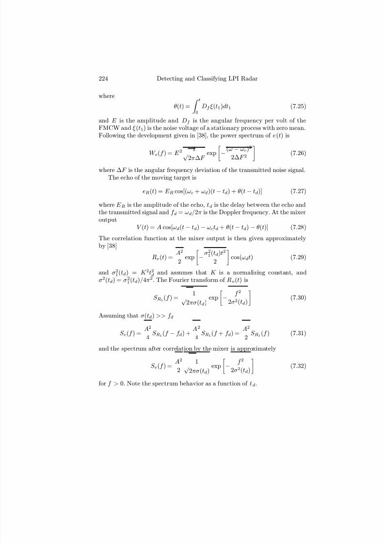
7/17/2019 1596932341 Intercept Radar.pdf
http://slidepdf.com/reader/full/1596932341-intercept-radarpdf 255/891
224 Detecting and Classifying LPI Radar
where
θ(t) =
t0
Df ξ (t1)dt1 (7.25)
and E is the amplitude and Df is the angular frequency per volt of theFMCW and ξ (t1) is the noise voltage of a stationary process with zero mean.Following the development given in [38], the power spectrum of e(t) is
W e(f ) = E 2 1√ 2π∆F
exp
− (ω − ωc)2
2∆F 2
(7.26)
where ∆F is the angular frequency deviation of the transmitted noise signal.The echo of the moving target is
eR(t) = E R cos[(ωc + ωd)(t− td) + θ(t− td)] (7.27)
where E R is the amplitude of the echo, td is the delay between the echo andthe transmitted signal and f d = ωd/2π is the Doppler frequency. At the mixeroutput
V (t) = A cos[ωd(t− td)− ωctd + θ(t− td) − θ(t)] (7.28)
The correlation function at the mixer output is then given approximatelyby [38]
Rv(t) = A2
2 exp
−σ21(td)t2
2
cos(ωdt) (7.29)
and σ21(td) = K 2t2d and assumes that K is a normalizing constant, andσ2(td) = σ21(td)/4π2. The Fourier transform of Rv(t) is
S R1(f ) =
1√ 2πσ(td)
exp
− f 2
2σ2(td)
(7.30)
Assuming that σ(td) >> f d
S v(f ) = A2
4 S R1
(f − f d) + A2
4 S R1
(f + f d) = A2
2 S R1
(f ) (7.31)
and the spectrum after correlation by the mixer is approximately
S v(f ) = A2
2
1√ 2πσ(td)
exp
− f 2
2σ2(td)
(7.32)
for f > 0. Note the spectrum behavior as a function of td.

7/17/2019 1596932341 Intercept Radar.pdf
http://slidepdf.com/reader/full/1596932341-intercept-radarpdf 256/891
Noise Techniques 225
Figure 7.9: Model of random noise plus FMCW transmitter (from [36]).
7.5.2 Model of RNFR Transmitter
A block diagram of the RNFR transmitter is shown in Figure 7.9 [36]. AMATLAB model of the RNFR is also contained in the LPIToolbox. Indi-cated on the diagram in parentheses are the places where intermediate resultsof the model are shown below. A wideband microwave noise generator firstproduces a signal that is band-limited to 300 MHz (200 ≤ f ≤ 500 MHz)centered at f c = 350 MHz. After bandlimiting, the noise signal modulates
a triangular FMCW signal with a modulation bandwidth ∆F = 300 MHzand modulation period tm = 1μs. The magnitude of the FMCW signal inFigure 7.9 (1) with ∆F = 300 MHz, and f c = 350 MHz are shown inFigure 7.10. The resultant signal is then high-pass-filtered to remove thelower sideband modulation leaving the transmitted signal with B = 600 MHz.The final noise modulated FMCW signal with ∆F = 300 MHz, and f c = 350MHz is shown in Figure 7.11. In Figure 7.12 the magnitude of the noiseFMCW high-pass filter output signal in Figure 7.9 (3) is shown (transmittedwaveform) with ∆F = 300 MHz and f c = 350 MHz.
7.5.3 Periodic Ambiguity Results
Using the same signal duration as in Section 7.4, the ACF and the PACFof the RNFR waveform are shown in Figure 7.13. For the RNFR waveformthe peak side lobes occur at approximately −21 dB down from the main lobeshowing the advantages of the FMCW modulation over a strictly randomnoise modulation. To examine the side lobe performance in the delay-Doppler

7/17/2019 1596932341 Intercept Radar.pdf
http://slidepdf.com/reader/full/1596932341-intercept-radarpdf 257/891
226 Detecting and Classifying LPI Radar
Figure 7.10: Magnitude of the FMCW signal shown in Figure 7.9 (1) with∆F = 300 MHz, and f c = 350 MHz.
Figure 7.11: Magnitude of the noise modulated FMCW signal in Figure 7.9(2) with ∆F = 300 MHz, and f c = 350 MHz.

7/17/2019 1596932341 Intercept Radar.pdf
http://slidepdf.com/reader/full/1596932341-intercept-radarpdf 258/891
Noise Techniques 227
Figure 7.12: Magnitude of the noise FMCW high-pass filter output signal inFigure 7.9 (3) with ∆F = 300 MHz, and f c = 350 MHz.
off set domain the PAF is then calculated and is shown in Figure 7.14. ThePAF main lobe repeats every code period or 6,000 samples. Note that thezero delay Doppler side lobes are also less compared to the RNR results. As afinal note for comparison, closed form expressions for the average ambiguity
function for the RNFR waveform are given in [38].
7.6 Random Noise FMCW Plus Sine
The random noise FMCW plus sine radar (RNFSR) uses an additional sinesignal at a frequency of f m that modulates the noise source [8]. The com-posite signal is then modulated by the FMCW waveform. The additionalsine signal that is added helps minimize the leakage from the transmitter tothe receiver as explained below. A block diagram of the RNFSR is shown inFigure 7.15. The receiver is similar to the RNFR receiver with the receivedsignal correlated to a time-delayed version of the emitted waveform using amixer. The mixer output contains the noise and all the sinusoidal harmonics.
The amplifi
er is a wideband automatic gain control circuit with a large dy-namic range [7]. To account for the injected sine wave, the receiver uses twobandpass filters to expand the receiver’s frequency range for the Doppler plusnoncorrelation signal and for the noncorrelation signal only. The transmitted

7/17/2019 1596932341 Intercept Radar.pdf
http://slidepdf.com/reader/full/1596932341-intercept-radarpdf 259/891
228 Detecting and Classifying LPI Radar
Figure 7.13: Random noise plus FMCW autocorrelation function and periodicautocorrelation function.
Figure 7.14: Random noise plus FMCW periodic ambiguity function.

7/17/2019 1596932341 Intercept Radar.pdf
http://slidepdf.com/reader/full/1596932341-intercept-radarpdf 260/891
Noise Techniques 229
signal for the RNFSR is [38]
ec(t) = E cos[ωct + θ1(t) + θ2(t)] (7.33)
where
θ1(t) =
t0
∆F cos(ωmt1)dt1 = D1 sin(ωmt) (7.34)
with
D1 = ∆F
ωm(7.35)
and
θ2(t) =
t0
Df V (t2)dt2 (7.36)
where the variable Df is the angular frequency per volt and V (t2) is themodulated noise voltage of a normal stationary process with zero mean andωm is the additional tone frequency. As expected, the derivation of the mixeroutput spectrum for the RNFSR is considerably more complicated and thereader is referred to [7].
The major diff erence between the RNFR and the RNFSR are the filtersshown in Figure 7.15. The filters have bandwidths expanded to include mul-tiples of the added sine signal within the return signal. The bandwidth of thefirst bandpass filter is selected to be B1 = nf m + f dmin and the bandwidthof the second bandpass filter is selected to be B2 = nf m + f dmax where nrepresents the nth harmonic of the added sine waveform that is picked upby the radar. This technique takes advantage of the harmonic characteris-
tics of the sinusoidal signal to eliminate the CW leakage at and close to zerorange [7—9]. This zero range hole characteristic does not let the radar respondto close-in targets and only produces an output detection when a target ispresent between the two chosen ranges determined by the filter bandwidths.Even with the addition of the sinusoidal modulation, the RNFSR cannot mea-sure the speed of a moving target or detect a long-range target (similar tothe RNFR). The RNFSR is suitable for short-range LPI applications such asharbor control, missile fuse systems and UAV landing systems.
7.6.1 Model of RNFSR Transmitter
The RNFSR noise technology employs an additional tone signal that is mod-ulated by the white Gaussian noise, which further modulates the FMCW
waveform. Figure 7.16 shows a block diagram of the transmitter modelused in this chapter [36]. A microwave noise generator produces a whiteGaussian noise waveform. After this, the signal is band-limited to 300 MHz,centered on f c = 350 MHz. After band-limiting, the noise signal is added(added in frequency, multiplied in time) to a single tone with a frequency of f m = 350 MHz. The upper band is centered at 700 MHz (from the modulation

7/17/2019 1596932341 Intercept Radar.pdf
http://slidepdf.com/reader/full/1596932341-intercept-radarpdf 261/891
230 Detecting and Classifying LPI Radar
Figure 7.15: Random noise FMCW plus sine radar block diagram (from [9]).
product) and this new signal modulates an FMCW signal with a modulationbandwidth of ∆F = 300 MHz. After noise modulation, the resultant signal islow-pass-filtered to remove the upper sideband modulation products. Finally,the 600-MHz bandwidth signal with center frequency of 350 MHz is amplifiedbefore transmission.
To examine the model development, Figure 7.17 shows the noise sourcewith the added tone modulation f m = 350 MHz. Note the frequency shiftof the waveform to a center frequency of 700 MHz. Figure 7.18 showsthe magnitude spectrum of the FMCW signal that is used to modulatethe noise with the added tone. The signal has a modulation bandwidth of ∆F = 300 MHz. In Figure 7.19, the modulation of the sine plus noise by theFMCW signal is shown. Shown are the resulting upper and lower sidebandproducts. The upper sideband is not needed and eliminated. Figure 7.20shows the magnitude spectrum of the output waveform.
7.6.2 Periodic Ambiguity Results
For the RNFSR transmitted waveform, a sine wave is added to the noise plusFMCW modulation. To compare the side lobe performance of this waveformwith the other noise modulations, the autocorrelation function and periodic
autocorrelation function are shown in Figure 7.21 for a 2-μs period of thewaveform. In this case the peak side lobe level is approximately −21 dB.Note that the side lobe structure is nearly the same as the RNFR waveformand the peak side lobe is not the first side lobe. The periodic ambiguityfunction is shown in Figure 7.22. Of interest here is the lower Doppler sidelobe level and the smaller extent of the Doppler side lobes.

7/17/2019 1596932341 Intercept Radar.pdf
http://slidepdf.com/reader/full/1596932341-intercept-radarpdf 262/891
Noise Techniques 231
Figure 7.16: Random noise FMCW plus sine transmitter model (from [36]).
Figure 7.17: Sine plus random noise FMCW model in Figure 7.16 showing(1) the magnitude spectrum of the tone modulation of noise.

7/17/2019 1596932341 Intercept Radar.pdf
http://slidepdf.com/reader/full/1596932341-intercept-radarpdf 263/891
232 Detecting and Classifying LPI Radar
Figure 7.18: Sine plus random noise FMCW model in Figure 7.16 showing(2) the magnitude spectrum of FMCW signal.
Figure 7.19: Sine plus random noise FMCW model in Figure 7.16 showing (3)the magnitude spectrum of noise plus sine after modulation by the FMCWsignal.

7/17/2019 1596932341 Intercept Radar.pdf
http://slidepdf.com/reader/full/1596932341-intercept-radarpdf 264/891
Noise Techniques 233
Figure 7.20: Sine plus random noise FMCW model in Figure 7.16 showing(4) the magnitude spectrum of output waveform after eliminating the uppersideband.
Figure 7.21: Sine plus random noise FMCW autocorrelation and periodicautocorrelation function.

7/17/2019 1596932341 Intercept Radar.pdf
http://slidepdf.com/reader/full/1596932341-intercept-radarpdf 265/891
234 Detecting and Classifying LPI Radar
Figure 7.22: Sine plus random noise FMCW periodic ambiguity function.
7.7 Random Binary Phase Modulation
The random binary phase code (RBPC) emitter is also a correlation CW
noise radar that uses a random phase modulation of a carrier frequency toachieve LPI noise characteristics. The range resolution of a RBPC CW emit-ter depends on the width of the subcode as
∆R = ctb
2 (7.37)
and the maximum range performance is
Rmax = N cctb
2 (7.38)
The Doppler tolerance depends on the length of the pulse compressor as
f dmax = 1
2N ctb(7.39)
where N c is the number of phase codes and tb is the subcode width. Note thatsimultaneously extending the Doppler tolerance and the range performanceis not possible since they are inverse relationships.
To improve the performance of the RBPC emitter, several pulse compres-sors can be used in series. A block diagram of this RBPC emitter is shown in
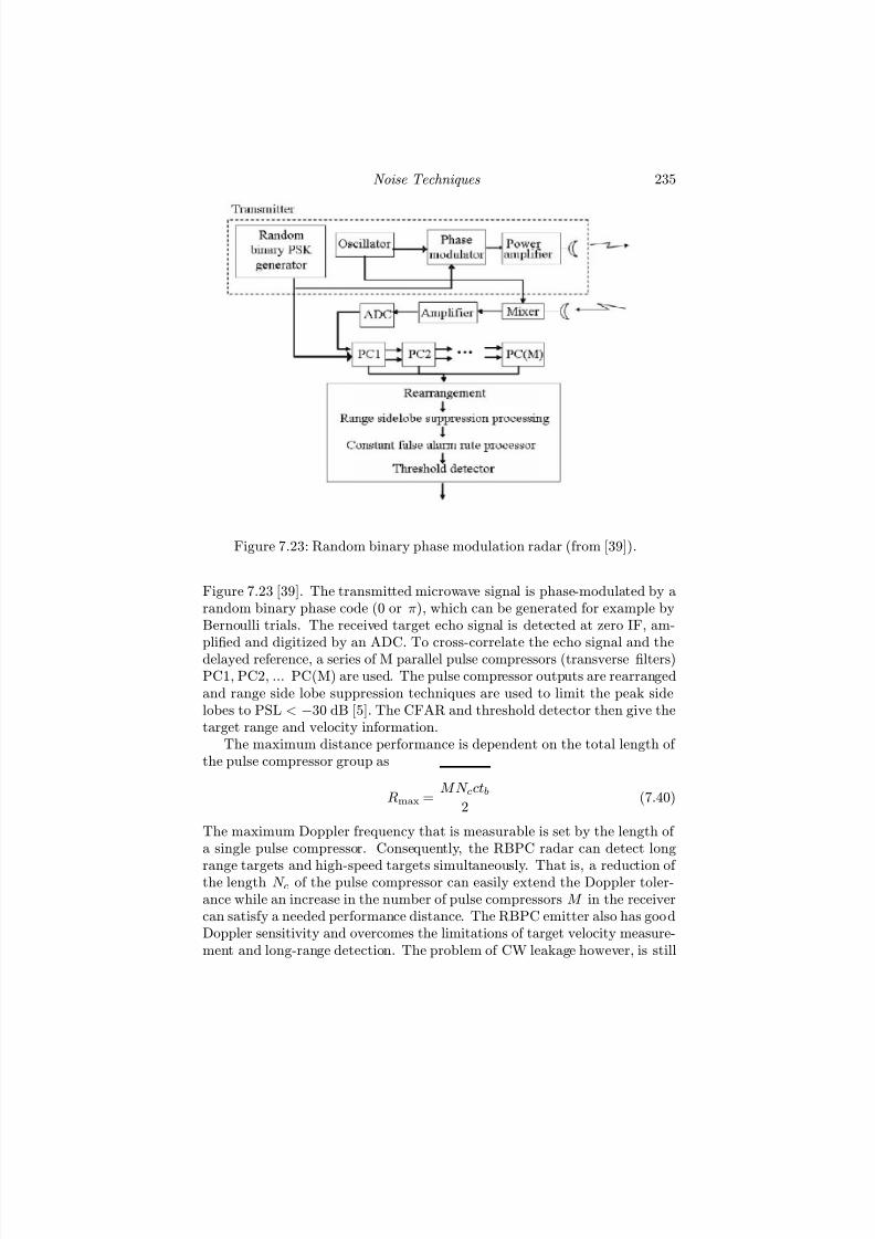
7/17/2019 1596932341 Intercept Radar.pdf
http://slidepdf.com/reader/full/1596932341-intercept-radarpdf 266/891
Noise Techniques 235
Figure 7.23: Random binary phase modulation radar (from [39]).
Figure 7.23 [39]. The transmitted microwave signal is phase-modulated by arandom binary phase code (0 or π), which can be generated for example byBernoulli trials. The received target echo signal is detected at zero IF, am-plified and digitized by an ADC. To cross-correlate the echo signal and thedelayed reference, a series of M parallel pulse compressors (transverse filters)PC1, PC2, ... PC(M) are used. The pulse compressor outputs are rearrangedand range side lobe suppression techniques are used to limit the peak sidelobes to PSL < −30 dB [5]. The CFAR and threshold detector then give thetarget range and velocity information.
The maximum distance performance is dependent on the total length of the pulse compressor group as
Rmax = M N cctb
2 (7.40)
The maximum Doppler frequency that is measurable is set by the length of a single pulse compressor. Consequently, the RBPC radar can detect long
range targets and high-speed targets simultaneously. That is, a reduction of the length N c of the pulse compressor can easily extend the Doppler toler-ance while an increase in the number of pulse compressors M in the receivercan satisfy a needed performance distance. The RBPC emitter also has goodDoppler sensitivity and overcomes the limitations of target velocity measure-ment and long-range detection. The problem of CW leakage however, is still
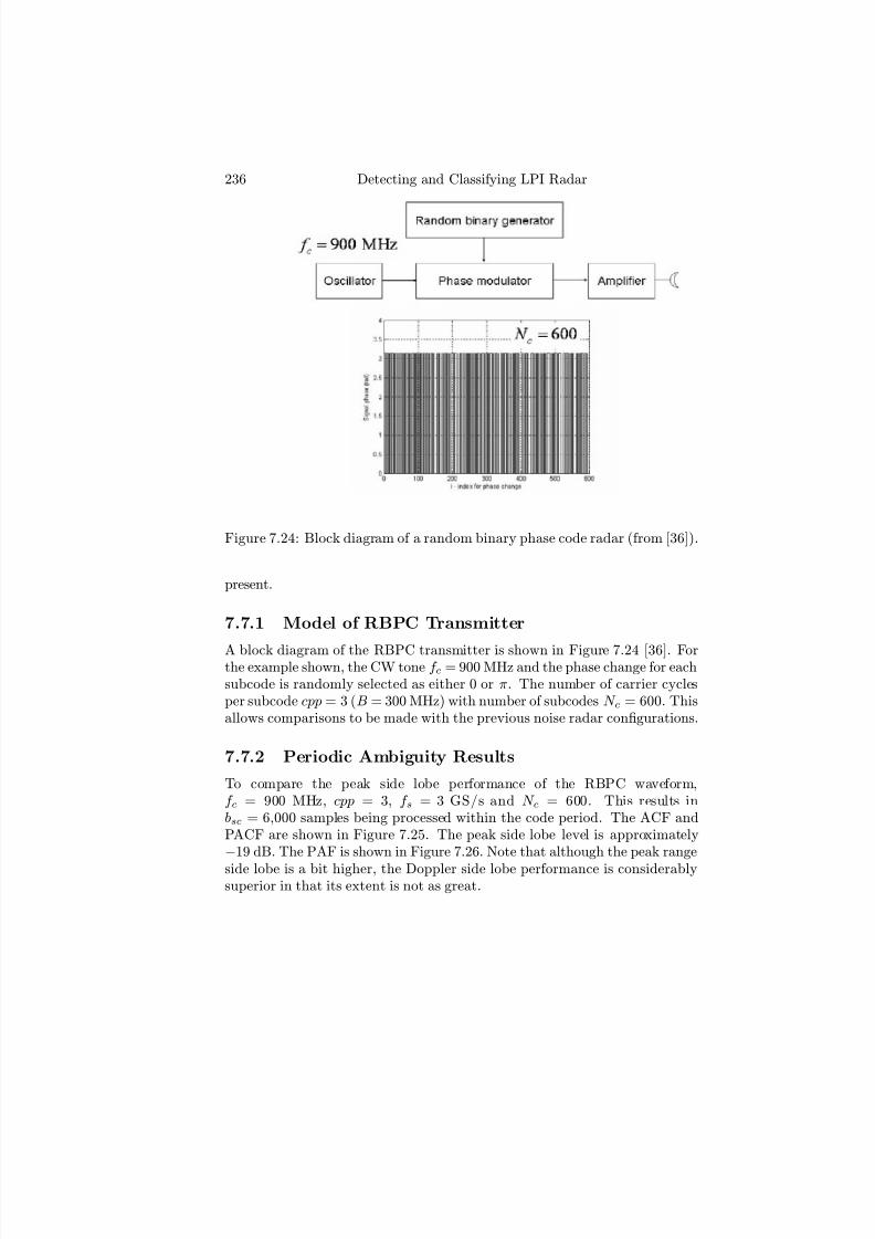
7/17/2019 1596932341 Intercept Radar.pdf
http://slidepdf.com/reader/full/1596932341-intercept-radarpdf 267/891
236 Detecting and Classifying LPI Radar
Figure 7.24: Block diagram of a random binary phase code radar (from [36]).
present.
7.7.1 Model of RBPC Transmitter
A block diagram of the RBPC transmitter is shown in Figure 7.24 [36]. Forthe example shown, the CW tone f c = 900 MHz and the phase change for eachsubcode is randomly selected as either 0 or π. The number of carrier cyclesper subcode cpp = 3 (B = 300 MHz) with number of subcodes N c = 600. Thisallows comparisons to be made with the previous noise radar configurations.
7.7.2 Periodic Ambiguity Results
To compare the peak side lobe performance of the RBPC waveform,f c = 900 MHz, cpp = 3, f s = 3 GS/s and N c = 600. This results inbsc = 6,000 samples being processed within the code period. The ACF andPACF are shown in Figure 7.25. The peak side lobe level is approximately
−19 dB. The PAF is shown in Figure 7.26. Note that although the peak range
side lobe is a bit higher, the Doppler side lobe performance is considerablysuperior in that its extent is not as great.
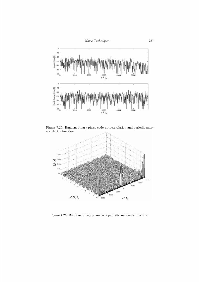
7/17/2019 1596932341 Intercept Radar.pdf
http://slidepdf.com/reader/full/1596932341-intercept-radarpdf 268/891
Noise Techniques 237
Figure 7.25: Random binary phase code autocorrelation and periodic auto-correlation function.
Figure 7.26: Random binary phase code periodic ambiguity function.

7/17/2019 1596932341 Intercept Radar.pdf
http://slidepdf.com/reader/full/1596932341-intercept-radarpdf 269/891
238 Detecting and Classifying LPI Radar
7.8 Millimeter Wave Noise RadarMillimeter wave (MMW) signals are most appropriate for applications such asenvironment monitoring, remote sensing, short range target detection, vehiclecollision warning and automatic landing systems [40]. Several MMW solid-state noise transmitters have been investigated. These systems rely on theuse of a chaotic waveform generator as a source of CW noise and a digital-analog correlator with an electronically controllable delay line as the mainpart of the correlation receiver. Three MMW noise sources were investigated.Dynamical chaotization2 was undertaken for: (1) microwave oscillations ina waveguide multiresonant system (2—5 resonant frequencies) containing oneor more Gunn-diodes that can couple two or more modes, (2) microwaveoscillations in a microstrip ring or linear resonator, and (3) angle modulation
of a VCO signal by an RF noise signal [41].Ka- and W-band solid state noise generators have also been developed
on the principles of chaotization of nonlinear systems using both IMPATT-and Gunn-diodes. Power outputs on the order of 300 mW with bandwidthsranging from 30 MHz to 300 MHz were generated. Special designs havealso been tested off ering bandwidths up to 2 GHz with an output power of 40 maw. To process the received signal from the target, fast digital real-timecorrelators were developed with clock frequencies on the order of 500 MHz.The use of ADCs were avoided by using a simple two-level quantization of the reference signal.
7.9 Correlation Receiver Techniques
The received noise signal reflected from the target is the delayed version of the transmitted signal. By measuring the delay, the receiver can determinethe location of the target. To compute the position of the target, the receivercomputes the cross-correlation between the time delayed, conjugated transmitsignal and the received signal. The analog cross-correlation function is definedas in (7.5). The correlation coefficient or normalized correlation function isdefined as in (7.17). Signals are said to be correlated or alike to the extent thattheir correlation coefficient approaches unity. Below we examine the diff erentapproaches to implementing the cross-correlation function in the receiver.
It can be shown that the received target response is a convolution betweenthe target reflectivity profile γ (t) and the ACF of the radar transmit waveform
p(τ ) [42]
g(τ ) = γ (t)⊗ p(τ ) (7.41)where
p(τ ) = limT →∞
T/2−T/2
S (t)S ∗(t− τ )dt (7.42)
2Chaotization is the theoretical and experimental study of chaos in dynamical systems.

7/17/2019 1596932341 Intercept Radar.pdf
http://slidepdf.com/reader/full/1596932341-intercept-radarpdf 270/891
Noise Techniques 239
If there is a point scatterer at a distance R, with amplitude a0 and initialphase φ0, the target reflectivity function can be expressed as
γ (t) = a0ejφ0δ (t− td) (7.43)
where δ denotes the Dirac impulse function.With the radar transmit waveform a band limited Gaussian noise signal
with carrier frequency f c, bandwidth B, and a square spectrum with powerσ2, the ACF is given by
p(τ ) = σ2sinc(Bτ )ej2πf cτ (7.44)
That is, for a radar that uses a band-limited Gaussian noise waveform as thetransmit signal, its ACF is a sinc-pulse modulated by the carrier frequencyf c [14].
7.9.1 Ideal Correlation
Figure 7.27 shows the block diagram of an ideal analog correlation receiver.The receiver consists of a noise source and an ideal time delay line thatproduces a delayed copy of the transmit signal. A mixer followed by a lowpassfilter performs the correlation integration between the received target returnsand the delayed transmit signals. The response is generated using an I & Qdemodulator. The cross-correlation function for the ideal analog correlationreceiver has been shown to be [42]
C I (τ ) = a0σ2sinc(Bτ )e(j2πf cτ −φ0) (7.45)
and preserves both the target amplitude and the initial phase.
7.9.2 Digital-Analog Correlation
A digital-analog correlation receiver is shown below in Figure 7.28 [42]. Inthis architecture, the delay line is implemented with a digital radio frequencymemory (DRFM) device. These devices use high-speed sampling and fast dig-ital memory for storing and replicating the transmitted RF noise signal. Theyprovide the ability to capture the transmitted signal and generate a precise,coherent replica for use in the correlation process. In the DRFM, the signal isdigitized and then multiplexed into high-speed dual-ported memory for stor-age and delay processing [43]. The delayed signal is then converted back toan analog signal using a digital-to-analog converter before being sent to themixer and lowpass filter. Expressed as a function of C I , the cross-correlation
function of a digital-analog cross-correlation with a 2N −level ADC is [42]
C DA(τ ) = a0πσ
N i=0
e−i2∆2
2σ2 C I (τ ) (7.46)
where ∆ is the quantization step size.

7/17/2019 1596932341 Intercept Radar.pdf
http://slidepdf.com/reader/full/1596932341-intercept-radarpdf 271/891
240 Detecting and Classifying LPI Radar
Figure 7.27: Ideal analog correlation receiver (from [42]).
Figure 7.28: Digital-analog correlation receiver (after [42]).

7/17/2019 1596932341 Intercept Radar.pdf
http://slidepdf.com/reader/full/1596932341-intercept-radarpdf 272/891
Noise Techniques 241
Figure 7.29: Fully digital correlation receiver. (After [42].)
7.9.3 Fully Digital Correlation
A fully digital cross-correlation receiver can also be used. In this configura-tion, both the received target echo signal and the copy of the transmit signalare digitized and the cross-correlation is done digitally. A block diagram of this approach is shown in Figure 7.29.
To avoid the use of ADCs, the principle of two level quantization of thereference signal has been proposed. Fast correlator hardware can be developedsince only the monobit (two-level) version of the noise waveform reference isdelayed in a fast controllable digital delay line made up of shift registers or fastrandom access memory. For the case when the delayed transmit signal andthe received signal are both clipped to be either −1 or +1 before performingcorrelation, the cross-correlation function has been shown to be [42]
C D(τ ) = 2
π sin−1[sinc(Bτ )] (7.47)
Work on fast digital signal processing algorithms for computation of the
cross-correlation are of high interest recently since this presents the majorcomputational burden in random noise radar. By increasing the samplesize N being processed, the requirements for the discrete Fourier transformprocessors and fast convolution processors which calculate the cross-correlationincrease sharply. Recently a system of orthogonal real-imaginary basis func-tions representing a new version of Walsh functions were compared to using a

7/17/2019 1596932341 Intercept Radar.pdf
http://slidepdf.com/reader/full/1596932341-intercept-radarpdf 273/891
242 Detecting and Classifying LPI Radar
set of Walsh Cooley functions for calculating the correlation [44]. Parametricand nonparametric algorithms are compared in [45].
7.9.4 Acousto-Optic Correlation
Due to the physical delay lines that are used a limited number of range bins isavailable. This either limits the range gate extent (maximum detectable rangescanned by the variable delay line) or the range resolution must be sacrificed.In addition, the slow switching speed (several seconds) of the variable delaylines can limit the data acquisition rate and constrain the ability to do real-time signal processing. This ultimately limits the ability to do range-Dopplerprocessing to detect fast moving targets.
Acousto-optic (AO) devices are well known for their utility in correlation
processing [46]. The use of an AO processor off ers another approach to corre-lation processing in the random noise radar. The receiver still employs a fiberoptic fixed-delay line to choose the coarse range delay but an acousto-optic(AO) time-integrating correlator is used to allow parallel range bin process-ing [47]. Here the received signal is heterodyned using the AO as the timeintegrating correlation receiver as shown in Figure 7.30. The noise signal istransmitted through the transmit antenna and the replica of the transmitted
Figure 7.30: Acousto-optic correlation receiver for noise radar (from [47]).

7/17/2019 1596932341 Intercept Radar.pdf
http://slidepdf.com/reader/full/1596932341-intercept-radarpdf 274/891
Noise Techniques 243
noise signal is delayed in the fixed fiber delay line (sets minimum detectablerange). After addition of a fixed bias and level adjustments, the signal mod-ulates the laser diode of the AO correlator. The laser diode light is thencollimated with a lens and focused on the AO device.
The received signal is used to drive a piezoelectric transducer, whichlaunches a traveling acoustic wave into the AO device. The correlation of thedelayed transmit and received signal is achieved by imaging the AO deviceaperture onto a 1-D CCD. The time-integrated correlation signal is producedby detecting the interference between the undiff racted beam and the polar-ization switched, diff racted traveling wave received signal by projecting bothoptical beams through a polarizer that can be rotated to optimize the beamratio for good interferometric modulation depth. The correlator provides theamplitude as a function of range as A = I 2 + Q2. Further details andexperimental results can be found in [47].
The use of the AO crystal provides up to 1,000 range cells that worksimultaneously over the aperture of the crystal providing the capability forreal-time data acquisition. The sensitivity is also improved up to 60 dB.Dynamic range and linearity are limited by the acoustic nonlinearities andscattering and by the limited dynamic range of CCD but could be increased byimproved CCD detector arrays providing higher bit resolution (e.g., 16 bits).There is also a noise figure penalty for the electrical to fiber to electricalconversion in the fiber delay line and AO correlator. This was off set by theprocessing gain achieved by the long integration time.
7.10 Concluding Remarks
Today noise waveforms can be generated digitally followed by a digital-to-analog converter and up-conversion onto a carrier signal. With the increasingintegration of solid-state microwave techniques and high-speed VLSI circuits,the correlation signal processing required for noise radar is leading the wayto real-time range-Doppler implementation. They are also relatively inex-pensive to build and there is considerable interest in relating the technologyto military applications such as covert surveillance and reconnaissance, tar-get detection and tracking, through-the-wall imaging, ground-penetration,foliage-penetration profiling, synthetic aperture radar and inverse syntheticaperture imaging.
The use of wideband noise waveforms can result in high resolution andreduced ambiguities in range and Doppler estimation. The periodic ambi-guity analysis for the four noise technology emitters are compared in thisChapter. Table 7.1 summarizes the peak range side lobe level (in dB) andthe peak Doppler side lobe level of the noise radar configurations simulatedin this chapter. These results do not include any side lobe suppression tech-niques which can lower these values significantly. The use of noise waveforms

7/17/2019 1596932341 Intercept Radar.pdf
http://slidepdf.com/reader/full/1596932341-intercept-radarpdf 275/891
244 Detecting and Classifying LPI Radar
can result in a large mismatch in processing gain between the radar and thenoncooperative intercept receiver making their presence hard to detect. Themost significant consequence on the traditional intercept receiver is a slightincrease in the receiver’s noise floor. Finally, the use of several noise wave-forms in a netted radar configuration can minimize the mutual interferencebetween emitters while providing an increase in surveillance volume and alsolowering the CW power required even further (see Chapter 9).
Table 7.1: Summary of Ambiguity Peak Side Lobe PerformanceNoise Technique Range Side Lob e Doppler Side Lob e
RNR (Figures 7.6 and 7.7) −3 dB −6RNFR (Figures 7.13 and 7.14) −21 dB −6
RNFSR (Figures 7.21 and 7.22) −
21 dB −
7RBPC (Figures 7.25 and 7.26) −19 dB −2
References
[1] Horton, B. M., “Noise-modulated distance measuring system,” Proceedings of the IRE , Vol. 49, No. 5, pp. 821—828, May 1959.
[2] Craig, S. E., Fishbein, W. and Rittenbach, O. E., “Continuous-wave radarwith high range resolution and unambiguous velocity determination,” IRE Transactions MIL-6 , pp. 153, April 1962.
[3] Grant, M. P., Cooper G. R., and Kamal, A. K., “A class of noise radarsystems,” Proceedings of the IEEE Vol. 51, No. 7, pp. 1060—1061, July, 1963.
[4] Cooper, G. R., and McGillem, C. D., “Random Signal Radar,” Final ReportNASA Grant-NSG 543, Purdue University, Lafayette, IN, June 1967.
[5] McGillem, C. D., Cooper, G. R., and Waltaman, W. B., “An experimentalrandom signal radar,” Proceedings of the National Electronics Conference ,Dayton, Ohio, pp. 409—411, Oct. 1967.
[6] Smit, J. A., and Kneefel, W. B. S. M., “RUDAR—An experimental noiseradar,” De Ingenieur, Vol. 83, No. 32, ppm. 99-110, Aug. 1971.
[7] Guosui, L., Hong, G., and Weimin, S., Hongbo, S., Jianhui, Z., “RandomSignal Radar—A Winner in Both the Military and Civilian Operating Envi-ronments,” IEEE Trans. on Aerospace and Electronic Systems , Vol. 39, No.2, pp. 489—498, April 2003.
[8] Guosui, L., Hong, G., Xiaohua, Z., and Weimin, S., “The Present and Future
of Random Signal Radars,” IEEE Aerospace and Electronic Systems Maga-zine, Vol. 12, No. 10, pp. 35—40, October 1997.
[9] Guosui, L., Hong, G., and Weimin, S., “Development of random signal radars,”IEEE Transactions on Aerospace and Electronic Systems , Vol. 35, No. 3, pp.770—777, July 1999.

7/17/2019 1596932341 Intercept Radar.pdf
http://slidepdf.com/reader/full/1596932341-intercept-radarpdf 276/891
Noise Techniques 245
[10] Garmatyuk, D. S., and Narayanan, R. M., “ECCM Capabilities of anUltrawideband Bandlimited Random Noise Imaging Radar,” IEEE Trans. on Aerospace and Electronic Systems , Vol. 38, No. 4, pp. 1243—1255, October2002.
[11] Xianyi, Z., Weimin, S., and Hong, G., “Anti-jamming performance analysisfor random noise UWB imaging radar,” Proceedings of the International Conf.on Radar (CIE ’06), Shanghai, China, 16—19 Oct. 2006.
[12] Turner, L., “The evolution of featureless waveforms for LPI communications,”Proceedings of the NAECON , Dayton, OH, pp. 1325—1331, May 1991.
[13] Axelsson, S. R. J., “Random noise radar/sodar with ultrawideband wave-forms,” IEEE Trans. on Geoscience and Remote Sensing , Vol. 45, No. 5, pp.1099—1114, May 2007.
[14] Narayanan, R. M., and Dawood, M., “Radar Penetration Imaging UsingUltra-wideband Random Noise Waveforms,” IEEE Trans. on Antennas and Propagation , Vol. 48, No. 6, pp. 868—878, June 2000.
[15] Lai, C-P., Ruan, Q., and Narayanan, R. M., “Hilbert-Huang transform (HHT)processing of through-wall noise radar data for human activity characteriza-tion,” Proceedings of the IEEE Workshop on Signal Processing Applications for Public Security and Forensics (SAFE), Washington DC, April 2007.
[16] Xu, X., and Narayanan, R. M., “FOPEN SAR Imaging Using UWB Step-Frequency and Random Noise Waveforms,” IEEE Trans. on Aerospace and Electronic Systems , Vol. 37, No. 4, pp. 1287—1300, October 2001.
[17] Xu, Y., and Narayanan, R. M., “Polarimetric Processing of Coherent RandomNoise Radar Data for Buried Object Detection,” IEEE Trans. on Geoscience and Remote Sensing , Vol. 39, No. 3, pp. 467—478, March 2001.
[18] Bell, D. C., and Narayanan, R. M., “Inverse synthetic aperture radar imagingusing a coherent ultrawideband random noise radar system,” Optical Engi-neering , Vol. 40, No. 11, pp. 2612—2623, November 2001.
[19] Garmatyuk, D. S., and Narayanan, R. M., “Ultra-Wideband Continuous-Wave Random Arc-SAR,” IEEE Trans. on Geoscience and Remote Sensing ,Vol. 40, No. 12, pp. 2543—2552, December 2002.
[20] Zhang, Y., and Narayanan, R. M., “Design Considerations for a Real-TimeRandom-Noise Tracking Radar,” IEEE Trans. on Aerospace and Electronic Systems , Vol. 40, No. 2, pp. 434—445, April 2004.
[21] Zhang, Y., and Narayanan, R. M., “Monopulse radar based on spatiotemporalcorrelation of stochastic signals,” IEEE Trans. on Aerospace and Electronic Systems , Vol. 42, No. 1, pp. 160—173, Jan. 2006.
[22] Zhang, Y., Narayanan, R. M., and Xu, X., “Theoretical and simulation analy-sis of random noise monopulse radar,” Proceedings of the IEEE Antennas and Propagation Symposium , San Antonio, TX, pp. 386—389, July 2002.
[23] Donnet, B. J., and Longstaff , I. D., “MIMO radar, techniques and oppor-tunities,” Proceedings of the 3rd European Radar Conference , pp. 112—115,Manchester UK, Sept. 2006.

7/17/2019 1596932341 Intercept Radar.pdf
http://slidepdf.com/reader/full/1596932341-intercept-radarpdf 277/891
246 Detecting and Classifying LPI Radar
[24] Gray, D. A., and Fry, R., “MIMO noise radar — element and beam space com-parisons,” Proceedings of the International Waveform Diversity and Design Conference , Pisa Italy, pp. 344—347, June 2007.
[25] Zetik, R., Sachs, J. and Thoma, R. S., “UWB short range radar sensing,”IEEE Instrumentation & Measurement Magazine , Vol. 10, No. 2, pp. 39—45,April 2007.
[26] Sun, H. “Possible ultra-wideband radar terminology,” IEEE Aerospace and Electronic Systems Magazine , Vol. 19, No. 8, pp. 38, Aug. 2004.
[27] Sun, H. Lu, Y., and Guosui, L., ”Ultra-Wideband Technology and RandomSignal Radar: An Ideal Combination,” IEEE Aerospace and Electronic Sys-tems Magazine , Vol. 18, No. 11, pp. 3—7, November 2003.
[28] Dawood, M., and Narayanan, R. M., “Generalized wideband ambiguity func-
tion of a coherent ultrawideband random noise radar,” IEE Proceedings-F Radar, Sonar, Navigation Vol. 150, No. 5, pp. 379—386, Oct. 2003.
[29] Axelsson, S. R. J., “Noise Radar for Range/Doppler Processing and DigitalBeamforming using Low-bit ADC,” IEEE Trans. on Geoscience and Remote Sensing , Vol. 41, No. 12, pp 2703—2720, December 2003.
[30] Axelsson, S. R. J., “Noise Radar Using Random Phase and Frequency Mod-ulation,” IEEE Trans. on Geoscience and Remote Sensing Vol. 42, No. 11,pp. 2370—2384, Nov. 2004.
[31] Narayanan, R. M., Henning, J-A, and Dawood, M., “Enhanced detection of objects obscured by dispersive media using tailored noise waveforms,” Pro-ceedings of the SPIE Conf. on Detection and Remediation Technologies for Mines and Minelike Targets III , Orlando, FL, Vol. 3392, pp. 604—614, April1998.
[32] Narayanan, R. M., Xu, Y., Hoff meyer, P. D., and Curtis, J. O., “Design per-formance and applications of a coherent ultra-wideband random noise radar,”Optical Engineering , Vol. 37 No. 6, pp. 1855—1869, June 1998.
[33] Jiang, R., Wolfe, K. W., and Nguyen, L., “Low coherence fiber optics for ran-dom noise radar,” Proceedings of the IEEE Military Communications Con- ference (MILCOM), Los Angeles, CA, pp. 907—911, Oct. 2000.
[34] Li, Z., and Narayanan, R. M., “Doppler visibility of coherent ultrawidebandrandom noise radar systems,” IEEE Trans. in Aerospace and Electronic Sys-tems , Vol. 42, No. 3, pp. 904—916, July 2006.
[35] Dawood, M., and Narayanan, R. M., “Receiver operating characteristics forthe coherent UWB random noise radar,” IEEE Trans. on Aerospace and Electronic Systems , Vol. 37, No. 2, pp. 586—594, April 2001.
[36] Heuschel, E. R., III, “Time-Frequency, Bi-Frequency Detection Analysis of Noise Technology Radar,” U. S. Naval Postgraduate School Master’s Thesis,Sept. 2006.
[37] Liu, G., and Xiangquan, S., “Average ambiguity function for random FM-CW radar signal,” International Conference on Radar , Paris, pp. 339—346,21—24 May 1984.

7/17/2019 1596932341 Intercept Radar.pdf
http://slidepdf.com/reader/full/1596932341-intercept-radarpdf 278/891
Noise Techniques 247
[38] Guosui, L., Xiangquan, S., Jinhui, L., Guoyu, Y., and Yaoliang, S., “Designof noise FM-CW radar and its implementation,” IEE Proceedings-F Radar,Sonar, Navigation , Vol. 138, No. 5, pp. 420—426, October 1991.
[39] Hong, G., Guosui, L., Xiaohua, Z., Weimin, S., and Xi, L., “A new kind of noise radar—random binary phase coded CW radar,” Proceedings of the IEEE National Radar Conference , Syracuse, NY, pp. 202—206, May 1997.
[40] Lukin, K. A., “Millimeter wave noise radar technology,” Proceedings of the 3rd International Symposium on Physics and Engineering of Microwave, Mil-limeter Wave and Submillimeter Waves , Kharkov Ukraine, Sept. 15—17, 1998.
[41] Lukin, K. A., “Millimeter wave noise radar applications: Theory and Exper-iment, Proceedings of the 4th International Symposium on Physics and Engi-neering of Microwave, Millimeter Wave and Submillimeter Waves , KharkovUkraine,, June 4—9, 2001.
[42] Xu, X., and Narayanan, R. M., “Impact of diff erent correlation receiving tech-niques on the imaging performance of UWB random noise radar,” Proceed-ings of the IEEE International Geoscience and Remote Sensing Symposium,IGARSS , Toulouse, France pp. 4525—4527, 21—25 July, 2003.
[43] Pace, P. E., Advanced Techniques for Digital Receivers , Artech House, Nor-wood, MA, 2000.
[44] Sinitsyn, R. B., and Beletsky, A. J., “Fast signal processing algorithms fornoise radar,” Proceedings of the 3rd European Radar Conference , Manchester,U.K., pp. 245—248, Sept. 2006.
[45] Yanovsky, F. J., and Sinitsyn, R. B., “Ultrawideband signal processing algo-rithms for radar and sodars,” Proceedings of the Ultrawideband and Ultrashort Impulse Signals , Sevastopol, Ukraine, pp. 66—71, 18—22 Sept. 2006.
[46] Hecht, D., “Characteristics of acoustooptic devices for signal processing,”Proceedings of the IEEE Symposium on Ultrasonics , San Francisco, CA, pp.369—380, 1985.
[47] Narayanan, R. M., Zhou, W., Wagner, K. H., and Kim, S., “AcoustoopticCorrelation Processing in Random Noise Radar,” IEEE Geoscience and Re-mote Sensing Letters , Vol. 1, No. 3, pp. 166—170, July 2004.
Problems
1. Determine the instantaneous fractional bandwidth of a noise waveformif the absolute bandwidth B = 3 GHz and the maximum bandwidthf max = 4 GHz.
2. Consider a moving target. The instantaneous Doppler frequency is nota constant but varies due to the varying nature of the instantaneouswavelength λ. Since λ varies between λmin and λmax, the Doppler fre-quencies vary from f dl to f dh. If f dc = (f min + f max)/2 is the average

7/17/2019 1596932341 Intercept Radar.pdf
http://slidepdf.com/reader/full/1596932341-intercept-radarpdf 279/891
248 Detecting and Classifying LPI Radar
Doppler corresponding to transmit frequency of f c, (a) show that theminimum and maximum Doppler frequency are
f dl = 2f minf dcf min + f max
(7.48)
and
f dh = 2f maxf dcf min + f max
(7.49)
(b) Derive the expression for the target’s velocity as a function of f dland also as a function of f dh. (c) Calculate f dl, f dh and the target’svelocity if λmin = 0.15m and λmax = 0.3m.
3. Show that a transmitted noise signal (7.11)
S t(t) = ReS (t) = X (t) cos(2πf ct) − Y (t) sin(2πf ct) (7.50)
can be expressed as
S t(t) = 1
2[sc(t)e2πf ct + s∗c(t)e−2πf ct] (7.51)
where sc(t) = X (t) + jY (t) is the complex conjugate envelope and ∗
denotes the complex conjugate.
4. Using the algorithms in the noise folder, generate the four types of noisewaveforms discussed in the chapter. Examine the ACF, PACF and PAFof each waveform and compare the highest time side lobe and Dopplerside lobe level (in dB) for each waveform.

7/17/2019 1596932341 Intercept Radar.pdf
http://slidepdf.com/reader/full/1596932341-intercept-radarpdf 280/891
Chapter 8
Over-the-Horizon Radar
In this chapter, we examine the sky wave over-the-horizon radar (OTHR)
concept including the characteristics of the ionosphere on the propagation of the radio waves and the clutter spectrum. Sky wave processing and modernLPI waveform considerations are presented. The sky wave maximum detec-tion range is also quantified for the Chinese OTH-B. Simulation results usingPROPLAB PRO, an ionospheric radio propagation tool published by SolarTerrestrial Dispatch, are shown to demonstrate the coverage region of theemitter. Surface wave OTHR are also presented including the LPI waveformconsiderations. The surface wave radar equation is developed and simula-tion results of the maximum detection range are shown as a function of therequired input SNR.
8.1 Two Types of OTHR
Today, many countries require an OTHR to provide a long-range, wide areasurveillance capability due to modern day terrorists, smugglers and the needto monitor one’s economic zone and off shore resources [1]. OTHR systemsoperate in the high frequency (HF) band 3—30 MHz and use either surface
wave propagation or sky wave propagation. Sky wave OTHR systems areinstalled inland and make use of the ionospheric refraction of the radio wavesseveral hundred kilometers above the Earth’s surface to overcome the line-of-sight limitation caused by the Earth’s curvature. Surface wave systemsoperate in the lower part of the HF spectrum and are installed on the coast-lines to make use of electromagnetic coupling of the emitted radio waves tothe sea surface allowing propagation to extend over the horizon. OTHR sur-face wave systems were considered first and operated in the early 1950s with
eff ective sky wave systems coming along later [2]. Although work on sky wave
249

7/17/2019 1596932341 Intercept Radar.pdf
http://slidepdf.com/reader/full/1596932341-intercept-radarpdf 281/891
250 Detecting and Classifying LPI Radar
OTH radars continues around the world, systems that exploit surface wavepropagation are attracting greater long-term interest due to their more con-venient size and transportability. The significant diff erence between sky waveand surface wave radars is that sky wave radars have large detection rangesbeyond the horizon (starting at about 800 km and extending out to 1,000—4,000 km) while surface wave systems can see out to 400 km. The reason forthe extended detection range for the sky wave propagation is that the lossescaused by the ionization and absorption in the ionosphere are much less thanthe surface wave diff raction loss. Ionospheric eff ects such as multipath andDoppler spreading are also significant. Targets such as cruise missiles, stealthaircraft, ballistic missiles and aircraft carriers can be detected with OTHRsystems at distances well beyond the horizon.
Several types of emitter waveforms for OTHR have been used in the past.Transmitted waveforms such as a simple pulse (e.g., cosine-squared), a chirpedpulse or a pulse Doppler waveform have been used [3]. Due to the very small
duty cycles, large peak powers were required to overcome the propagationlosses incurred. With the necessity of having to operate across bands inwhich other authorized users were emitting many anti-interference measureshad to be included [2]. The high-power, pulsed waveforms eff ectively detectedthe targets however, they allowed the long-range interception of the emitterby noncooperative intercept receivers leading to direction finding, emitteridentification, electronic attack (jamming), and deception.
In order to provide a more covert military capability as well as a more effi-cient use of the HF spectrum, the modern OTHR is moving towards the use of CW LPI waveform modulations such as CW phase modulation and frequencyhopping [4]. Low power FMCW using multiple waveform repetition frequen-cies [5, 6] are being used that can relax the transmit power requirements toprovide a more covert sky wave system. In addition these types of waveforms
can resolve the range/Doppler ambiguity usually associated with HF FMCWradar. Surface wave systems using random low power FM interrupted CW(FMICW) are also being pursued [7]. The FMICW is a FMCW waveformthat is gated on and off either randomly or with a well-defined sequence.The main problem caused by the spectra discontinuity is the high-range sidelobes. Optimal sparse waveform designs [8] are being explored. They findthe interference-free channels in the HF band by frequency monitoring, en-abling the target detection to be accomplished using clear channels while alsolowering the transmit power and minimizing the range side lobes. Shortercoherent integration times (CIT) [9], adaptive transmit frequency techniques[10], antijamming through the use of a radar waveform with discontinuousspectra using two carrier frequencies [11] and orthogonal MIMO waveforms[12] are also resulting in a quieter and more eff ective OTHR.
The ionospheric propagation and movement of the layers, contaminatesthe transmitted waveform resulting in a low, and fading SNR at the target.Traditionally, anti-interference measures such as adaptive frequency tuning,

7/17/2019 1596932341 Intercept Radar.pdf
http://slidepdf.com/reader/full/1596932341-intercept-radarpdf 282/891
Over-the-Horizon Radar 251
adaptive filtering (including tunable band reject filters) and spatial filteringhave been used by the emitter [2]. Modern OTHR signal processing tech-niques such as adaptive interference suppression [13—15] and clutter cance-lation algorithms [16] are now able to eliminate the ionospheric propagationpath contaminants and compensate for the smearing of sea echo very eff ec-tively. Adaptive time-frequency analysis has also been used to parameterizethe radar signal so the interference can be identified and removed [17].
On the other hand, the ionospheric propagation makes the noncooperativedetection of the OTHR more difficult. The ionospheric contamination makesthe polarization at the receiver indeterminable and consequently, the detec-tion and DF (azimuth and elevation estimates) of the OTHR waveforms istricky especially in the presence of the other interference within the HF band[18]. The antenna aperture required is large in size and must also be usefulacross the HF band with no grating lobes. Large shipboard multifunction ar-rays are hampered by limitations on the physical size of the aperture required
and problems with electromagnetic interference and compatibility [19]. Sin-gle sight location techniques using complex time delay estimation algorithmshave been used to DF the OTHR signals [20]. Furthermore, the received HFsignals are nonstationary which limits the noncoherent integration efficiencywithin the signal processing. Due to multipath presence, high-resolution spec-tral estimation techniques such as multiple signal classification (MUSIC) andthe cepstrum must also be used [18].
Since the HF signals have a large wavelength (10 ≤ λ ≤ 100m) the OTHRalso has an inherent resistance to the ARM threat. This is because HFwavelengths are greater than 10m and any antenna mounted in a missileseeker (diameter = 0.5m) would have significant difficulty deriving any usefulguidance information from the emitted HF waveform. In addition to counter-ARM capacity, the HF CW waveforms can also detect stealth aircraft and
low level penetrators providing strategic and long distance early warning1
[21].The OTHR systems are able to survey large areas of land and sea for air andmaritime targets. The OTHR’s operating wavelength is nearly the same sizeas many of the targets being pursued which puts the targets in the resonantscattering region (increase in RCS and target detection performance).
In this chapter, sky wave OTHR systems and the eff ect the ionospherehas on the waveforms is presented. LPI waveforms are discussed and PRO-PLAB PRO simulation results are shown to demonstrate the typical footprintcoverage as a function of the HF frequency. Example results for the ChineseOTH-B system are shown. MATLAB simulations showing the maximumdetection range as a function of the minimum required SNR are also dis-cussed. Surface wave systems are examined including the FM interruptedCW approach. With the focus on new emitter waveforms, incorporation of
electronic protection, signal processing and spectrum management, the inter-1Stealth aircraft are not optimized against bistatic over-the-horizon radars.

7/17/2019 1596932341 Intercept Radar.pdf
http://slidepdf.com/reader/full/1596932341-intercept-radarpdf 283/891
252 Detecting and Classifying LPI Radar
Figure 8.1: Sky wave radar concept (adapted from [23]).
ception and direction finding (DF) of both the sky wave and surface waveOTHR systems present a significant challenge. For a review of the world’sOTHR systems, see [22].
8.2 Sky Wave OTHR
The emitted waveform from the sky wave OTHR system is bounced off
theionosphere and then down to the targets. Reflections from the targets arebounced back through the ionosphere to the receiver array as shown in Fig-ure 8.1 [23]. Note the similarity to the MIMO (or spatially waveform diverse)architecture as discussed in Chapter 10. Due to the amount of sea clutterbeing returned the term backscatter is often used. Use of the term backscat-ter is intended to identify the system geometry, in which the small separationbetween transmitter and receiver results in an eff ective monostatic radar, asopposed to a bistatic geometry in which the large angle between the transmitand receive path modifies the target and clutter RCS. These backscatter sys-tems consist of two modes for detection of targets. Detection of air targets,and ballistic missiles during the launch phase constitute an air mode . Detec-tion of surface targets is called a surface mode . Although they are typically
separate operating modes, eff orts to combine the modes is also being pursued.Both modes are aff ected significantly by the ionosphere and these eff ects arepresented below.

7/17/2019 1596932341 Intercept Radar.pdf
http://slidepdf.com/reader/full/1596932341-intercept-radarpdf 284/891
Over-the-Horizon Radar 253
Figure 8.2: Temperature and plasma density of neutral gas and ionized gasas a function of altitude (after [25]).
8.2.1 Characteristics of the Ionosphere
The ionosphere is defined as that part of the upper atmosphere where suffi-cient ionization can exist to aff ect the propagation of radio waves [24]. Ex-amining the LPI characteristics of OTHR systems requires an understandingof the ionosphere and its eff ects. The structure of the neutral atmosphereand the ionosphere containing ionized gas surrounding the Earth is shown inFigure 8.2 [25]. The left side of the figure (neutral gas) shows the altitude (inkilometers) as a function of temperature (in Kelvin). The layer right abovethe Earth’s surface up to 10 km is the troposphere and all weather phenomenaoccur here. The layer above the troposphere is the stratosphere and the airflow is horizontal. The layer above the stratosphere is the mesosphere where
the temperature increases with altitude. The layer above the mesosphere isthe ionosphere. The right side of Figure 8.2 (ionized gas) shows the altitude
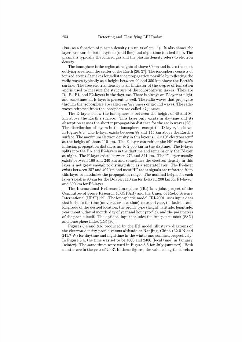
7/17/2019 1596932341 Intercept Radar.pdf
http://slidepdf.com/reader/full/1596932341-intercept-radarpdf 285/891
254 Detecting and Classifying LPI Radar
(km) as a function of plasma density (in units of cm−3). It also shows thelayer structure in both daytime (solid line) and night time (dashed line). Theplasma is typically the ionized gas and the plasma density refers to electrondensity.
The ionosphere is the region at heights of above 80 km and is also the mostoutlying area from the center of the Earth [26, 27]. The ionosphere consists of ionized atoms. It makes long-distance propagation possible by reflecting theradio waves typically at a height between 90 and 350 km above the Earth’ssurface. The free electron density is an indicator of the degree of ionizationand is used to measure the structure of the ionosphere in layers. They areD-, E-, F1- and F2-layers in the daytime. There is always an F-layer at nightand sometimes an E-layer is present as well. The radio waves that propagatethrough the troposphere are called surface waves or ground waves. The radiowaves refracted from the ionosphere are called sky waves .
The D-layer below the ionosphere is between the height of 48 and 80
km above the Earth’s surface. This layer only exists in daytime and itsabsorption causes the shorter propagation distance for the radio waves [28].The distribution of layers in the ionosphere, except the D-layer, is shownin Figure 8.3. The E-layer exists between 88 and 145 km above the Earth’ssurface. The maximum electron density in this layer is 1.5×10⁵ electrons/cm3
at the height of about 110 km. The E-layer can refract the HF radio waveinducing propagation distances up to 2,000 km in the daytime. The F-layersplits into the F1- and F2-layers in the daytime and remains only the F-layerat night. The F-layer exists between 273 and 321 km. The F1-layer usuallyexists between 160 and 240 km and sometimes the electron density in thislayer is not great enough to distinguish it as a separate layer. The F2-layerexists between 257 and 402 km and most HF radar signals are refracted fromthis layer to maximize the propagation range. The nominal height for each
layer’s peak is 90 km for the D-layer, 110 km for E-layer, 200 km for F1-layer,and 300 km for F2-layer.
The International Reference Ionosphere (IRI) is a joint project of theCommittee of Space Research (COSPAR) and the Union of Radio ScienceInternational (URSI) [29]. The ionospheric model, IRI-2001, uses input datathat includes the time (universal or local time), date and year, the latitude andlongitude of the desired location, the profile type (height, latitude, longitude,year, month, day of month, day of year and hour profile), and the parametersof the profile itself. The optional input includes the sunspot number (SSN)and ionosphere index (IG) [30].
Figures 8.4 and 8.5, produced by the IRI model, illustrate diagrams of the electron density profile versus altitude at Nanjing, China (32.0 N and241.7 W) for daytime and nighttime in the winter and summer, respectively.
In Figure 8.4, the time was set to be 1000 and 2400 (local time) in January(winter). The same times were used in Figure 8.5 for July (summer). Bothmonths are in the year of 2007. In these figures, the value along the abscissa

7/17/2019 1596932341 Intercept Radar.pdf
http://slidepdf.com/reader/full/1596932341-intercept-radarpdf 286/891
Over-the-Horizon Radar 255
Figure 8.3: Distribution of layers in the ionosphere during the daytime andnighttime.
(from left to right) represents the electron density (electrons/cm3) for each al-titude. The electron density is generated by semilog calculation method. The
numbers along the ordinate of the figure correspond to the altitude above theground (in kilometers). The first three lines on the top of the graph representthe information of the geographic coordinates, time, day, and month. Thefourth line shows the optional inputs, SSN and IG index, that are generatedby the model itself unless input by the user. In the daytime results shownin Figure 8.4(a) and Figure 8.5(a), the D, E and F2-layers are easily defined,but the F1-layer is not well defined. In the night time results shown in Figure8.4(b) and Figure 8.5(b), both E and F-layer are well defined. These resultsdemonstrate that the successful noncooperative interception of the OTHRwaveforms depend heavily on the conditions of the ionosphere, time of day,and sun spot number (SSN) as well as the emitter power and range.
Modeling the ionospheric electron density N e and refractive index μ isuseful for HF propagation studies and OTHR system planning and perfor-
mance prediction. Exploitation of this predictability by the targets can alsobe used to avoid detection by the OTHR (e.g., by flying when the propaga-tion losses and ionospheric modulation are the worst). The electron density
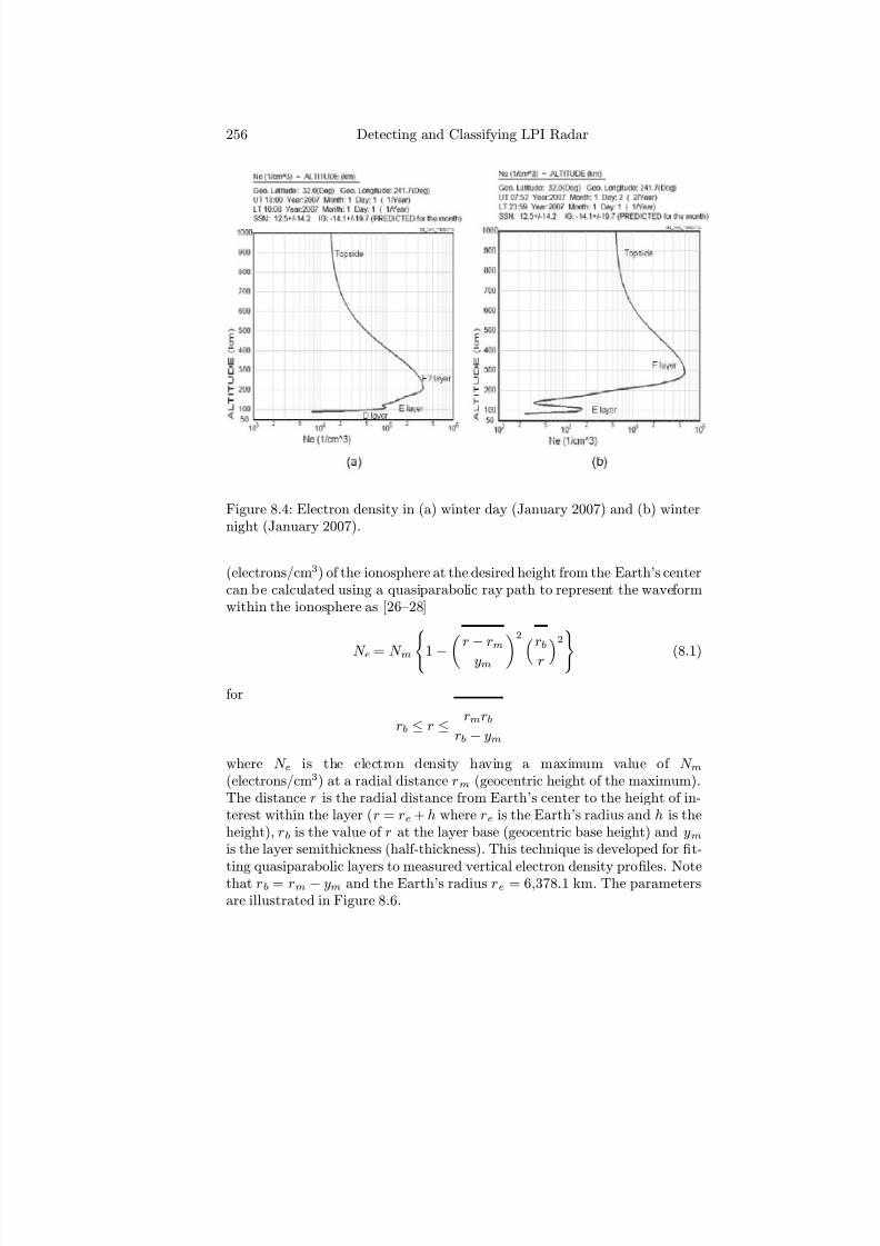
7/17/2019 1596932341 Intercept Radar.pdf
http://slidepdf.com/reader/full/1596932341-intercept-radarpdf 287/891
256 Detecting and Classifying LPI Radar
Figure 8.4: Electron density in (a) winter day (January 2007) and (b) winternight (January 2007).
(electrons/cm3) of the ionosphere at the desired height from the Earth’s centercan be calculated using a quasiparabolic ray path to represent the waveformwithin the ionosphere as [26—28]
N e = N m
1− r
−rm
ym2 rb
r2
(8.1)
for
rb ≤ r ≤ rmrbrb − ym
where N e is the electron density having a maximum value of N m(electrons/cm3) at a radial distance rm (geocentric height of the maximum).The distance r is the radial distance from Earth’s center to the height of in-terest within the layer (r = re + h where re is the Earth’s radius and h is theheight), rb is the value of r at the layer base (geocentric base height) and ymis the layer semithickness (half-thickness). This technique is developed for fit-
ting quasiparabolic layers to measured vertical electron density profi
les. Notethat rb = rm − ym and the Earth’s radius re = 6,378.1 km. The parametersare illustrated in Figure 8.6.

7/17/2019 1596932341 Intercept Radar.pdf
http://slidepdf.com/reader/full/1596932341-intercept-radarpdf 288/891
Over-the-Horizon Radar 257
Figure 8.5: Electron density in (a) summer day (July 2007) and (b) summernight (July 2007).
The critical frequency (kHz) is the maximum frequency of the emittedwaveform that is returned from a layer at normal incidence. That is, when theemitted waveform is transmitted straight up towards the ionosphere (verticalincidence), the waveform will be returned to earth at all frequencies belowthe critical frequency f cr (kHz) which takes the form [2]
f cr =
81N m (8.2)
Thus at normal incidence (φi = 0o) a wave will penetrate the ionosphere if f > f cr. A negative refractive index occurs when f < f cr and this resultsin a ray at normal incidence being reflected from the ionosphere to return tothe Earth. In case the frequency exceeds the critical frequency the influencethe ionosphere layer has on the path of propagation depends upon the angleof incidence φi at the ionosphere. The angle of incidence φi is measuredfrom the normal to the ionospheric layer. The critical frequency f cr is notthe highest frequency that can be reflected from the layer. The maximumfrequency that can be reflected back for a given distance of transmission iscalled the maximum usable frequency (MUF). The MUF is related to the
critical frequency and the angle of incidence by [31]
MUF = f cr secφi (8.3)
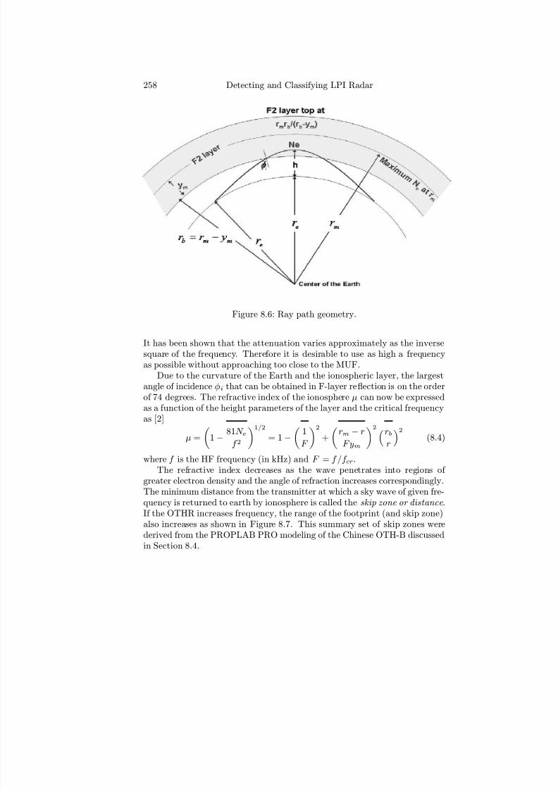
7/17/2019 1596932341 Intercept Radar.pdf
http://slidepdf.com/reader/full/1596932341-intercept-radarpdf 289/891
258 Detecting and Classifying LPI Radar
Figure 8.6: Ray path geometry.
It has been shown that the attenuation varies approximately as the inversesquare of the frequency. Therefore it is desirable to use as high a frequencyas possible without approaching too close to the MUF.
Due to the curvature of the Earth and the ionospheric layer, the largestangle of incidence φi that can be obtained in F-layer reflection is on the orderof 74 degrees. The refractive index of the ionosphere μ can now be expressedas a function of the height parameters of the layer and the critical frequencyas [2]
μ =
1− 81N e
f 2
1/2
= 1−
1
F
2
+
rm − r
F ym
2 rbr
2(8.4)
where f is the HF frequency (in kHz) and F = f /f cr.The refractive index decreases as the wave penetrates into regions of
greater electron density and the angle of refraction increases correspondingly.The minimum distance from the transmitter at which a sky wave of given fre-quency is returned to earth by ionosphere is called the skip zone or distance .If the OTHR increases frequency, the range of the footprint (and skip zone)also increases as shown in Figure 8.7. This summary set of skip zones werederived from the PROPLAB PRO modeling of the Chinese OTH-B discussedin Section 8.4.

7/17/2019 1596932341 Intercept Radar.pdf
http://slidepdf.com/reader/full/1596932341-intercept-radarpdf 290/891
Over-the-Horizon Radar 259
Figure 8.7: Coverage range for f c = 6, 8, 10, 12, 14, 16, 18, 20 and 22 MHz for
SSN = 200 and the AI = 5 on 0:00 UTC 2007/7/31 [22].
8.2.2 Example of F2-Layer Propagation
Consider the electron density profile for the summer daytime in Figure 8.5.Here the maximum electron density N m of the F2-layer is at the height of rm = 6618.1 km (240+6,378.1), with a value of 3 × 10⁵ electrons/cm3. TheF2-layer semithickness (half-thickness) ym = 50 km or ym = 0.5(300− 200),and the base height of the F2-layer rb = rm− ym or 6568.1 km, which meansthe base height of the F2-layer is 190 km above the Earth’s surface (also shownin Figure 8.5). At a desired height of 230 km above the Earth’s surface, theelectron density is calculated from (8.1) as N e = 2.8814 × 10⁵ electrons/cm3.The critical frequency depends only on the maximum electron density of the
F2-layer f cr = 4.93 × 10³ kHz. Based on (8.4), the refractive index μ isa function of electron density N e and operating frequency f (kHz). If afrequency of f = 5.1 × 10³ kHz is considered, the refractive index μ = 0.32.If the waveform is launched at an angle of incidence of φi = 10 degrees,MUF= 5 × 10³ kHz.
8.2.3 Doppler Clutter Spectrum
How the targets appear in the Doppler space relative to the clutter is im-portant in determining the HF frequency to be used. The excessive noisecaused by ionospheric propagation is due to the electron density variations.This process decorrelates the radio signal as it propagates and broadens theDoppler spectrum. The Doppler radar spectrum of HF radiation backscat-
tered from the ocean surface is shown in Figure 8.8 and characterized by twostrong peaks appearing above and below the carrier frequency [32]. The phys-

7/17/2019 1596932341 Intercept Radar.pdf
http://slidepdf.com/reader/full/1596932341-intercept-radarpdf 291/891
260 Detecting and Classifying LPI Radar
Figure 8.8: Bragg peaks along with air and surface targets within the clutter-target Doppler profile (after [32]).
ical mechanism producing this phenomenon is single-bounce Bragg scatteringfrom wave trains. The Bragg peaks represent the radiation being reflected.The Doppler frequencies of the Bragg peaks are ±0.102
√ f c Hz where f c is the
operating frequency in megahertz and the sign ± indicates the resonant oceanwaves advancing towards or receding away from the radar. The sidebands sur-rounding the Bragg peaks are due to wave-wave interactions and higher order
Bragg scattering [33]. The ocean properties that can be extracted from fea-tures of the HF radar sea echo spectrum include (from easiest to measure)radial surface currents, sea state, surface wind speed, dominant wave periodand direction [34].
Radial velocity variation of maneuvering targets (aircraft) with high speedmay cause significant spread on the radar echo in the Doppler spectrum.These eff ects make the echo energy disperse and degrades the efficiency of the coherent integration operation (coherent integration loss). Aircraft targetspeeds separate them well from surface targets and clutter for many geome-tries and provide a good match to the radar capabilities. Many ways havebeen proposed to deal with maneuvering targets in OTHR systems. For air-craft, the modulation periods are typically several seconds. Ships which haveradial speeds between 5 and 25 ms−1 require coherent modulation periods
longer than tens of seconds to achieve high resolution in the Doppler domainso as to distinguish the targets from the clutter [32]. The positioning accuracy

7/17/2019 1596932341 Intercept Radar.pdf
http://slidepdf.com/reader/full/1596932341-intercept-radarpdf 292/891
Over-the-Horizon Radar 261
can also be improved by the use of active transponders, clutter storage anddisplay technology (to calibrate coast lines) and the use of one transmittingsite and multiple receiving sites. Many targets of interest may be concealedby the clutter and this obscuration is predictable and hence exploitable byships wishing to evade detection. For OTHR, reducing the severity of cluttermasking is actively being investigated.
8.2.4 Example Sky Wave OTHR System
As an example, consider the Australia’s Jindalee Operational Radar Network.The Jindalee Over-the-horizon Radar Network (JORN) is a system that pro-vides surveillance over 4,000 km of Australia’s northern coastline. Full imple-mentation of JORN has involved the construction of two OTH backscatterradars that operate in the HF band and are able to detect airborne and shiptargets at ranges of between 1,000 and 3,000 km, with a range resolutionof 20—40 km. The JORN radars incorporate bistatic transmission and re-ception subsystems geographically separated to prevent mutual interference.The transmission subsystem comprises 28 transmitter chains, each of whichincorporates a 20-kW power amplifier [35].
The receiver subsystem near Longreach, Queensland utilizes 480 receiverchains, while the one near Laverton, Western Australia incorporates 960 suchchains. Figure 8.9 shows the JORN transmission site at Longreach, Queens-land. An integral frequency management system determines which frequencywithin the operating band will yield the best SNR while spectrum and noisemonitors identify clear channels and background noise levels. A backscat-ter sounder is used to monitor ionospheric propagation characteristics in thetarget area and operating frequency selection is made on the basis of inde-pendent data that is gathered. General ionospheric structure characteristics
and target ground truths are obtained via a network of vertical and obliquesounding facilities and transponders located along Australia’s northern coast-line [32]. The Longreach 3-km reception array is shown in Figure 8.10 andis positioned some 100 km from its associated transmitter. A JORN Coor-dination Center (JCC) is located at the Royal Australian Air Force (RAAF)base Edinburgh near Adelaide, South Australia. Here, the received data isprocessed into usable tracking data. The Longreach site is equipped with a0.4-km transmission array.
8.2.5 Sky Wave Processing
For sky wave systems, the receivers and transmitters are almost always sepa-rated by as much as 100 km or more. Sky wave systems have large immovable
antenna arrays that are spread out over a long distance and are positionedinland such that they are relatively immune to most forms of enemy attack byrockets and missiles. Sky wave OTHR transmitters use adaptive frequency

7/17/2019 1596932341 Intercept Radar.pdf
http://slidepdf.com/reader/full/1596932341-intercept-radarpdf 293/891
262 Detecting and Classifying LPI Radar
Figure 8.9: The JORN transmission site at Longreach, Queensland [35].
Figure 8.10: Jindalee receiving antenna [35].

7/17/2019 1596932341 Intercept Radar.pdf
http://slidepdf.com/reader/full/1596932341-intercept-radarpdf 294/891
Over-the-Horizon Radar 263
selection, low side lobe adaptive digital beam forming, and require sophisti-cated frequency management systems using ionosondes in order to operatevia the ever-changing ionosphere [32]. Ionosondes are devices that send aspectrum of radio wave pulses straight up to measure: (a) the length of timeit takes for a reflection to be returned, (b) the strength of the reflection, and(c) how high of a frequency can be reflected. From these three measurements(time, strength, frequency), the device can determine ionization density, al-titude of the ionization, and the MUF. The transmitting system is usuallyimplemented as a number of separate antenna arrays, each covering a certainfrequency subband. Due to the large area being illuminated, these systemsprovide the users with a significant surveillance capability to detect targetsat any altitude from the ionosphere to the surface of the Earth.
The receive antenna is usually a long (> 1 km) array of monopoles some-times with a backscreen to reduce the back lobe radiation. The receiverarray is connected to a beamformer, receiver and ADC. The receiver output
is digitized by an ADC and strobed into a bulk memory for target detectionprocessing. The samples within a range gate (all range bins of interest) areadded together coherently for a period of time that may vary anywhere fromseveral seconds to several minutes depending on the targets being detected.Beyond the time where coherent integration is performed, the returns fromthe sea may be added noncoherently. That is, since the samples from beyondthe horizon are stored digitally, a good deal of flexibility in the processingnow exists (mostly to correct for the ionospheric modulation of the Doppler).
Pulse OTHR systems use short pulses or pulse compression to obtain high-range resolution and a high peak power is required to obtain the necessaryaverage power for target detection. This high transmitted power can lead toantenna design constraints and gives rise to impulsive interference that caneasily be identified within the HF band. The engineering compromise to using
high peak power, low duty cycle waveforms is to use CW frequency sweepingsuch as the FMCW. Modern sky wave emitters for example, take advantageof low power (30W in the case of WERA [36]) FMCW modulation. Althoughthere is currently no military OTHRs that use tens or hundreds of W, thelow power emitted makes it easy for them to hide within other HF radioservices and interference. sky wave OTHRs for air vehicle detection must usemuch higher powers than 30W. JORN and the US OTH-B use hundreds of kW average power. The use of FMCW modulation to transmit and receivecontinuously maximizes the average power out of the transmitter’s amplifiersproviding the range resolution inherent in a given transmission bandwidth.
The disadvantages in using an FMCW are the spectral purity required inthe waveform generator and the high dynamic range required in the receiverwhich has to handle the strong direct path (transmit antenna to receive an-
tenna) and the weak signals from far ranges. Doppler information must alsobe derived by repeating the FM sweep a number of times (e.g., 64 or 128) andthen performing the FFT in each range gate to examine the phase history

7/17/2019 1596932341 Intercept Radar.pdf
http://slidepdf.com/reader/full/1596932341-intercept-radarpdf 295/891
264 Detecting and Classifying LPI Radar
of any target in that gate. After these repeated FMCW sweeps in any givendwell or surveillance time, the OTHR moves to survey other azimuths andranges that are part of the surveillance plan.
Due to the frequency range of OTHR systems and the low volume datarates, new digital receivers can now directly digitize the returned CW signalwith high resolution without the need for down conversion to intermediatefrequencies (as is conventionally done for microwave emitters). The signalprocessor uses a primary FFT to sort the echo returns into range bins and asecond FFT is used to calculate the range-Doppler map. For the OTHR, theunambiguous range of operation is given by [37]
Ru = c
2WRF (8.5)
where WRF is the waveform repetition frequency WRF = 1/tm Hz and tmis the modulation period. The range resolution depends on the modulation
bandwidth ∆F that is used. The return signals are accumulated over thisbandwidth which determines the range resolution. The range resolution (m)is given by
∆R = c
2∆F (8.6)
For a WRF, the blind speed which varies as a function of f c as [37]
ν = cWRF
2f c(8.7)
For the surface-mode (detection of ships), a narrow modulation bandwidth∆F is used with a high WRF. For the air-mode (detection of aircraft targets),a large modulation bandwidth is used with a smaller WRF. In both propaga-tion cases the amount of energy scattered from the target back to the radarreceiver is extremely small. In addition, the HF bandwidth used representsa wide percentage of the tunable bandwidth and the signals received afterpropagation are nonstationary.
Each region within the coverage area is illuminated with the FMCW andcoherent integration is performed over a number of modulation periods. Thecoherent integration time (CIT) must be long enough to extract the targetechoes. The CIT is variable to accommodate the changing ionospheric, clutterconditions, and target types. Illumination for a long CIT however, worksagainst the OTHR in terms of avoiding a noncooperative intercept. If the CITis too short however, the low Doppler resolution cannot separate the ship fromthe large ocean clutter. For the aircraft target, a short CIT is not a problemsince the speed separates it well from the clutter. A significant problem is
the robust high-resolution Doppler processing of accelerating or deceleratingtargets [38]. The waveform parameters that can be set include the WRF,the operating frequency, the modulation bandwidth and the CIT. Multiple

7/17/2019 1596932341 Intercept Radar.pdf
http://slidepdf.com/reader/full/1596932341-intercept-radarpdf 296/891
Over-the-Horizon Radar 265
WRFs are used while the target is being illuminated and this solves the rangeDoppler ambiguity. Multiple carrier frequencies (either simultaneous or timemultiplexed) are also used to enhance the target detection capability.
8.3 Sky Wave LPI Waveform Considerations
The repetitive nature of the frequency sweeping is one of the main drawbacksof the FMCW technique. The concentration of power into narrow HF band-widths and the additional element of repetition (e.g., with the same WRF)makes the OTHR vulnerable to detection, which can lead to electronic attackand deception. Consequently, the move away from these traditional wave-forms to the incorporation of new LPI modulations is being actively pursued.Changing the modulation parameters makes it even more difficult to DF theemitter and identify the OTHR system location.
8.3.1 Phase Modulation Techniques
Phase modulation CW techniques such as Barker binary phase coding (withlow time side lobes) have been considered [4]. For a coherent integration timeCIT, more than one modulation period is integrated. Including the CIT, thepeak side lobe level or PSL (see Chapter 3) is given by
PSL = 20log10
tb
WRF
(8.8)
For example, for a tb = 50 μs subcode width and WRF = 5 s, aPSL = −100 dB is available everywhere in the ambiguity space. Time domainweighting is used to control the Doppler side lobes at the zero range cut (at
the expense of Doppler resolution). Without weighting or uniform weighting,the zero-range cut follows the sinc pattern with −13 dB side lobes. Polyphasecodes are also being explored since they provide low side lobes without theuse of weighting. Using polyphase codes with N c subcodes
PSL = 20 log10
1
N c
(8.9)
For example, for N c = 64, PSL = −36 dB. The polyphase codes however,have a significant Doppler tolerance and therefore are not useful as a Dopplersensitive waveform. As discussed in Chapter 5, polyphase codes off er theLPI CW emitter good flexibility in achieving a large processing gain or time-bandwidth product and can be quite useful in OTHR systems.

7/17/2019 1596932341 Intercept Radar.pdf
http://slidepdf.com/reader/full/1596932341-intercept-radarpdf 297/891
266 Detecting and Classifying LPI Radar
8.3.2 Costas Frequency Hopping
Frequency hopping Costas codes are also being explored. The peak side lobe
level for a given Costas time-bandwidth product is
PSL = 20 log10
1
B(WRF)
(8.10)
For example, for B = 20 kHz and a WRF = 5 s, a PSL = 100 dB can beachieved in addition to a thumbtack ambiguity function.
Increasing the time-bandwidth product of these CW modulations usinglarger bandwidths is also being pursued entailing operations over a discon-tinuous signal spectrum (due to all of the other radio traffic), an approachsimilar to the surface wave techniques that are used.
8.3.3 Reducing the CIT
In addition to the goal of LPI, a surveillance plan to scan, detect and tracksurface targets over large areas requires a short CIT in order that the trackercan receive the periodic updates in a timely fashion. To enable a shortCIT, efficient clutter cancelation algorithms are actively being pursued toimprove signal-to-clutter ratio. Fourier-based clutter cancelation algorithmshave shown success for OTHR and are based on modeling the first order clut-ter as a sinusoid and subtracting it from the data. The Fourier techniqueestimates the clutter frequency, amplitude and phase [9] from the Dopplerspectrum. A high clutter-to-noise ratio for the Bragg peaks is required inorder to estimate the initial phase for the clutter subtraction.
8.3.4 Multiple Waveform Repetition Frequencies
Unlike a pulsed signal, with FMCW, an ambiguous Doppler frequency is notfolded within the same time delay resolution cell but is shifted to a nearbytime delay cell. Recall that this cross-coupling eff ect is the range-Doppler am-biguity of this waveform. One technique to overcome this ambiguity problem,which also leads to a more LPI waveform, is the use of multiple WRFs withina single illumination period [5]. It is also wellknown that ionospheric insta-bility noise (due to polar and equatorial regions) has the potential to appearthrough a range ambiguity on top of the signals of interest if the WRF ≥ 7.5Hz. This causes problems for aircraft which have Doppler frequencies of 5—60Hz. Consequently, Doppler frequencies greater than this must be resolvedwithout any range ambiguities.
To understand the use of multiple WRF technique, we revisit the FMCW
range-Doppler cross coupling eff ect as presented in Chapter 4. Recall thatthe beat frequency is proportional to the range of a stationary target (or one

7/17/2019 1596932341 Intercept Radar.pdf
http://slidepdf.com/reader/full/1596932341-intercept-radarpdf 298/891
Over-the-Horizon Radar 267
that has a Doppler shift f d < ±1/2t0) as
R =
cf bt0
2∆F (8.11)
and the corresponding range resolution
∆R = c
2∆F =
c∆tmin
2 (8.12)
where ∆tmin = 1/∆F s is the minimum time delay that can be detected.Due to the range-Doppler cross coupling eff ect, if the target is moving ata velocity such that f d > ±1/2t0, the beat frequency is f m = f b ± f d andcorresponding range of the target is given by
Rm = cf bt02∆F
± cf dt02∆F
(8.13)
and shows that the measured range is a function of the true range and anerror due to the Doppler shift or Rm = R ± Rd. The range error due to theDoppler shift can be re-written in terms of range bins as [5]
Rd
∆R= ±
f dWRF
(8.14)
where WRF = 1/t0. This shows that the measured range is increased (ordecreased) by one range bin as the Doppler shift is decreased (or increased)by a frequency equal to the WRF.
In the multiple WRF technique, three WRFs are used during a singletarget illumination time as shown in Figure 8.11. Since the waveform repeti-
Figure 8.11: Coprime waveform repetition frequencies.
tion frequencies of the waveforms are diff erent, aliasing causes the estimatedDoppler shifts to be diff erent during each WRF. The Chinese remainder the-
orem can then be utilized to calculate the true Doppler shift where the max-imum unambiguous Doppler range is limited by the least common multiple(LCM) of the selected WRFs [5, 6]. The duration and number of coprime

7/17/2019 1596932341 Intercept Radar.pdf
http://slidepdf.com/reader/full/1596932341-intercept-radarpdf 299/891
268 Detecting and Classifying LPI Radar
WRF sweeps are chosen to resolve the range ambiguities and to achieve therequired Doppler resolution respectively.
The Doppler shifts are unique for each WRF block and estimated sequen-tially using two FFTs as in normal FMCW processing. For OTHR surfacemode targets, it is only necessary to extend the unambiguous Doppler to±70 Hz so WRF3 = 7, WRF2 = 6, and WRF1 = 5 are sufficient giving amaximum unambiguous Doppler coverage of
f d = ±1
2
3i=1
WRFi = ±105 Hz (8.15)
In selecting the WRF, the first limitation is the maximum unambiguous range
Rmax ≤ctm3
2 <
ctm2
2 <
ctm1
2 (8.16)
where tmi are the corresponding modulation periods for the three WRFs(tmi = 1/WRFi) [6]. The diff erence in range bins between the three WRFsshould be large enough to separate the clutter. If N RB is the number of binscovered by the clutter then to ensure a clutter free range
N RB = ∆F
WRF1− ∆F
WRF2(8.17)
and also
N RB = ∆F
WRF2− ∆F
WRF3(8.18)
which is the smallest diff erence. Rewriting (8.18),
N RB∆F <
WRF3
−WRF2
WRF3WRF2 (8.19)
and choosing WRF3 = WRF2 + 1, (8.19) is then
∆F
N RB> WRF2
2 + WRF2 (8.20)
A fixed waveform repetition frequency emitter is able to resolve Doppler fre-quencies within ±WRFi/2. With the WRFi satisfying WRF3 > WRF2 >WRF1, the Doppler shift of the target can be written as [5]
f d = n1WRF1 + x1 = n2WRF2 + x2 = n3WRF3 + x3 (8.21)
where n1, n2 and n3 are either a positive or a negative integer depending on
the Doppler shifts and x1, x2 and x3 are the corresponding fractions that arethe measured Doppler shifts of certain targets with the limits −WRFi/2 ≤xi ≤ WRFi/2.

7/17/2019 1596932341 Intercept Radar.pdf
http://slidepdf.com/reader/full/1596932341-intercept-radarpdf 300/891
Over-the-Horizon Radar 269
Below we present the alternate solution using the Chinese remainder the-orem (CRT) and repeat the example in [5]. The problem is first set up as aset of simultaneous congruences
f d ≡ x1(mod WRF1)
f d ≡ x2(mod WRF2)
f d ≡ x3(mod WRF3) (8.22)
When WRFi are N positive integers that are coprime, the set of congruenceshave a unique solution modulo
M =N i=1
WRFi (8.23)
Any integer congruent modulo M to a given solution is also a solution. (Theproof and straightforward computation of the CRT is given in [39].) Thesolution of the simultaneous congruences is
f d =N j=1
M
WRFjbjxj (8.24)
or for N = 3
f 0 = WRF2WRF3b1x1 + WRF1WRF3b2x2 + WRF1WRF2b3x3(mod M )(8.25)
The bi values are found by a repeated application of the Euclidean algorithm.So to complete the CRT solution we consider the example given in [5] whereWRF1 = 5 Hz, WRF2 = 6 Hz, and WRF3 = 7 Hz and the correspondingambiguous Doppler shifts are x1 = 2 Hz, x2 = −2 Hz, and x3 = 3 Hz. Forb1, since the greatest common divisor of 42 (M/WRF1 = WRF2WRF3) and5 (WRF1) is 1, the Euclidean algorithm is used to solve for x0, y0 such that42x0 + 5y0 = 1. Then we have 42x0 ≡ 1(mod 5), so b1 = x0. Applying thealgorithm [39]
42(1) + 5(0) = 4242(0) + 5(1) = 542(1) + 5(−8) = 242(−2) + 5(17) = 1
and consequently, b1 = −2. Repeating the application of the Euclidean al-gorithm for b2 and b3 gives b2 = −1 and b3 = −3. The solution (8.25) isthen
f d = −4(42) + 70− 270(mod 210) = −368 (8.26)
which is out of the proper range (0 to 209). However, M = 210 goes into −368two times, so
−368 + 2(210) = 52 solves the problem and is the least positive
solution. That is f d = 52 Hz as also solved in [5]. The technique presentedhere determines the actual Doppler frequency and is a more straightforwardmethod using the CRT.

7/17/2019 1596932341 Intercept Radar.pdf
http://slidepdf.com/reader/full/1596932341-intercept-radarpdf 301/891
270 Detecting and Classifying LPI Radar
8.3.5 Out-of-Band Emission Suppression
In MIMO systems, the design objectives are transmitter element waveform
orthogonality (using either temporal or spectral diversity). The implemen-tation is limited by the performance of the transmission system especiallythe out-of-band emissions. New approaches to FMCW waveform design andto waveform generation have been adopted that are theoretically capable of achieving much lower out-of-band spectral levels [13]. Spectrum leakage thatis out of band can be a significant beacon for HF/DF systems trying to nonco-operatively identify the emitter. For FMCW sky wave emitters, out-of-bandemission suppression is a major consideration and steps are usually takento insure compliance with for example, the International TelecommunicationUnion (ITU). The ITU-R spectral management document SM.1541-1 providesrecommendations on out-of-band emission advice for a number of radar wave-forms including the FMCW waveform. The reduction of side lobes throughtime and frequency weighting can be done to improve the out-of-band emis-
sion spectrum while improving the in-band performance. One choice is tosmooth the frequency transition region at the ends of each chirp by smooth-ing the signal in either the instantaneous frequency or amplitude domains[14].
Recall that a single sawtooth FMCW signal frequency can be written inthe time domain as
f I (t) = ∆F
tmt + f c (8.27)
for |t| ≤ tm/2. The complex signal is then
v(t) = ejφ(t) (8.28)
where
φ(t) = π∆F tm
t2 + 2πf ct (8.29)
for |t| ≤ tm/2.The spectral taper method begins by designing the waveform in the spec-
tral domain and including a modulation with a taper function wST (f )
vfm =
∞
−∞
wST (f )v(f )ej2πftdt (8.30)
The function vfm can then be inverse Fourier transformed to derive the signal.Taper functions such as the Hann taper function have been used. The taperhowever, does change slightly, the signal’s phase, amplitude and instantaneousfrequency.
The instantaneous frequency of the FMCW waveform is also a discontin-uous function. A simple method to reduce this discontinuity is to introduce

7/17/2019 1596932341 Intercept Radar.pdf
http://slidepdf.com/reader/full/1596932341-intercept-radarpdf 302/891
Over-the-Horizon Radar 271
a counter sloping chirp at the waveform end as [14]
f I (t) = 1
1− γ ∆F
tm t + f c (8.31)
for −tm/2 ≤ t ≤ (1 − 2γ )tm/2 and f I (t) = −∆F t/(γ tm) + f c otherwise.Here 0 ≤ γ ≤ 1/2 is the flyback factor. The flyback factor accounts for theamount of time required for the sawtooth FMCW to return to the beginningfrequency. To reduce the roll-off rate the application of amplitude taperingcan be applied. For example, a cosine-Tukey amplitude taper wCT (t) in thetime domain on the signal takes the form
vam(t) = wCT (t)v(t) (8.32)
This technique provides excellent out-of-band emission control even with lowpercentage tapering (e.g., 10%) causing only a small amount of loss in coher-
ent gain.The penalty when using this approach is that the Fresnel ripples, whichare usually a characteristic of the spectrum of the weighted chirp signal, nowappear in the time domain waveform. The waveform to be transmitted hassmall amplitude ripples that must be preserved if the desired spectral perfor-mance is to be maintained [13]. That is, high linearity must be maintainedat full output power levels.
8.4 Sky Wave Maximum Detection Range
The relative performance of the best known sky wave OTHR systems is shownin Figure 8.12. One of the important performance parameters of the OTHRis the maximum detection range. Figure 8.13 shows the OTH-B sky wavetarget detection geometry. The received power at the radar receiver from thetarget can be expressed as
P RT = P CW GT GRλ
2σT
(4π)3R2T R
2RLP 2LF L
(8.33)
where P CW is the average transmitter power in watts, GT is the transmitantenna gain, GR is the receive antenna gain, λ is the wavelength at thecarrier frequency f c,
σT is the target’s radar cross-section, the term LP 2 is the two-way trans-mission path loss and is on the order of 10—20 dB [21], L is the system losseswhich include the transmitter and receiver subsystem losses which are 15 dB[23]. LF is the Faraday polarization loss of the ionosphere which is typically
3 dB [21], RT is the distance of the ray path traveling from the radar, re-flecting off of the ionosphere down to the target and RR is the distance of the return ray path traveling from the target to the receiver also reflecting

7/17/2019 1596932341 Intercept Radar.pdf
http://slidepdf.com/reader/full/1596932341-intercept-radarpdf 303/891
272 Detecting and Classifying LPI Radar
Figure 8.12: Relative performance of the best known sky wave OTHR systems(after [22]).
off of the ionosphere. Understanding the ionosphere, and how it aff ects thetransmit and received waveform (from the target) is critical to predicting theOTHR capability. For example, the ionosphere can modulate the target’sDoppler profile making it undetectable. This is discussed in greater detail inthe following sections.
The minimum input signal-to-noise ratio SNRRi is related to the receiver’ssensitivity δ R. The receiver can detect and process an incoming target signalat this signal level or higher. Substitution of the sensitivity for P RT in (8.34),the maximum detection range (reflecting off of the ionosphere) of the radarbecomes
RRmax =
P CW GT GRλ
2σT
(4π)3δ RLP 2LF L
1/4
(8.34)
where RRmax is calculated by assuming that the OTHR transmitter and re-ceiver are located at the same range from the target RT = RR. The sensitivityδ R is the product of the minimum SNR required at the input SNRRi timesthe noise power in the input bandwidth of the receiver or
δ R = kT 0F RBRi(SNRRi) (8.35)
where k is the Boltzmann’s constant (k = 1.3807×10⁻²³ J/K), T 0 is the stan-dard noise temperature (290 K), F R is the receiver noise factor and includes
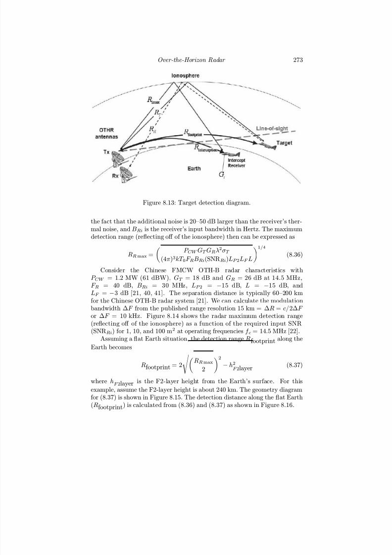
7/17/2019 1596932341 Intercept Radar.pdf
http://slidepdf.com/reader/full/1596932341-intercept-radarpdf 304/891
Over-the-Horizon Radar 273
Figure 8.13: Target detection diagram.
the fact that the additional noise is 20—50 dB larger than the receiver’s ther-mal noise, and BRi is the receiver’s input bandwidth in Hertz. The maximumdetection range (reflecting off of the ionosphere) then can be expressed as
RRmax =
P CW GT GRλ
2σT
(4π)3kT 0F RBRi(SNRRi)LP 2LF L
1/4
(8.36)
Consider the Chinese FMCW OTH-B radar characteristics withP CW = 1.2 MW (61 dBW), GT = 18 dB and GR = 26 dB at 14.5 MHz,F R = 40 dB, BRi = 30 MHz, LP 2 =
−15 dB, L =
−15 dB, and
LF = −3 dB [21, 40, 41]. The separation distance is typically 60—200 kmfor the Chinese OTH-B radar system [21]. We can calculate the modulationbandwidth ∆F from the published range resolution 15 km = ∆R = c/2∆F or ∆F = 10 kHz. Figure 8.14 shows the radar maximum detection range(reflecting off of the ionosphere) as a function of the required input SNR(SNRRi) for 1, 10, and 100 m2 at operating frequencies f c = 14.5 MHz [22].
Assuming a flat Earth situation, the detection range Rfootprint along the
Earth becomes
Rfootprint = 2
RRmax
2
2
− h2F 2layer (8.37)
where hF 2layer is the F2-layer height from the Earth’s surface. For this
example, assume the F2-layer height is about 240 km. The geometry diagramfor (8.37) is shown in Figure 8.15. The detection distance along the flat Earth(Rfootprint) is calculated from (8.36) and (8.37) as shown in Figure 8.16.

7/17/2019 1596932341 Intercept Radar.pdf
http://slidepdf.com/reader/full/1596932341-intercept-radarpdf 305/891
274 Detecting and Classifying LPI Radar
Figure 8.14: FMCW OTH-B maximum detection range (RRmax) for σT = 1,10, and 100 m2 [22].
From [21], the Chinese OTH-B radar has a skip zone or minimum detectionrange of 700 km and a maximum detection range of 3,500 km. For a maximumdetection range along the flat Earth Rfootprint = 3,500 km, the RRmax
is calculated as 3,532 km from (8.36). The minimum required input SNR(SNRRi) for f c = 14.5 MHz for σT = 1, 10, and 100 m2 is −107, −97 and
−87 dB respectively from Figure 8.16. The processing gain of the emitter’s
waveform used then provides the sufficient SNR for target detection.After target detection, coordinate registration is used for multipath track-
ing to convert the slant ranges and slant azimuth to surface coordinates.Several methods based on planar and spherical models have been reportedrecently [42—44]. Furthermore, with sophisticated processing to eliminate thecoherent integration loss caused by irregular target motions, the transmitpower can be lowered considerably.
8.5 Sky Wave Footprint Prediction
PROPLAB PRO is a propagation software for the personal computer thatcalculates the precise behavior of radio signals as they travel through theatmosphere. It simulates accurately, radio transmissions into the ionosphereusing sophisticated ionospheric ray-tracing techniques [45]. One of the OTHR

7/17/2019 1596932341 Intercept Radar.pdf
http://slidepdf.com/reader/full/1596932341-intercept-radarpdf 306/891
Over-the-Horizon Radar 275
Figure 8.15: Geometry diagram of the detection range calculation.
parameters that is of high interest to the noncooperative intercept receiver to
predict is the emitter footprint or coverage area. For the Chinese OTH-B radar, the transmitter is assumed to be located at Nanjing (32.05oN,241.22oW) and the target is located at coordinates 30oN, 204.3oW whichis 3,500 km distance away from the transmitter. A typical transmitter an-tenna radiation pattern is shown in Figure 8.17 with a maximum transmitgain of 18 dB at 14.5 MHz from a vertical dipole array pointed in azimuth85o from true North (towards the United States).
Simulation results for the summertime SSN 200 are shown below. Thelevel of geomagnetic activity (A-Index, AI) = 5 on 21 July 2007. The electrondensity profile (N e) at the midpoint ( 32.37oN, 222.55oW) of the transmitterand the target along the great-circle path is shown in Figure 8.18. The D, E,F2 and topside layers are shown.
The maximum usable frequency (MUF) profile (24-hour period) is shown
in Figure 8.19 with the F2-layer MUF (the top-most line), optimum workingfrequency or FOT (the second line), average MUF of E and F-layer (the thinline next to FOT line), and the E-layer MUF (the bottom line). The mostoften used frequency range is between the FOT and the average MUF of Eand F layer.
From Figure 8.19, the maximum and minimum FOT values are 28 MHz at08:00 UTC (coordinated universal time) and 20 MHz at 19:00 UT (universaltime). Based on the maximum and minimum FOTs, the ray tracing screenscan be generated as shown in Figures 8.20 and 8.21. To examine the footprintcoverage and the skip zones generated as a function of frequency and elevationangle, the ray trace plots for f c = 6, 8, 10, 12, 14, 16, 18, 20 and 22 MHz weregenerated for angles between 0o and 20o. For these results SSN = 200 andthe AI = 5 on 0:00 UTC 2007/7/31. Figure 8.20 shows the results for 10 MHzand 14 MHz. Two eff ects can be noticed from the results. First, the increaseof frequency toward the MUF results in an extended range and increased

7/17/2019 1596932341 Intercept Radar.pdf
http://slidepdf.com/reader/full/1596932341-intercept-radarpdf 307/891
276 Detecting and Classifying LPI Radar
Figure 8.16: FMCW OTH-B maximum detection range (Rfootprint) for σT =
1, 10, and 100 m2 [22].
skip zone. In addition, when going from f c = 10 MHz to f c = 14 MHz,the 20o elevation launch angle finally penetrates the ionosphere. In Figure8.7, a summary of the ray trace plots is shown. The range coverage for eachfrequency is shown (including the skip zone). Note that as the frequencyapproaches the MUF, the range increases. In Figure 8.21, f c = 18 MHz and
f c = 22 MHz are shown. Considerable ionospheric penetration is occurringfor SSN = 200 and the AI = 5 on 0:00 UTC 2007/7/31 as the frequencyapproaches the MUF.
8.6 Surface Wave OTHR
While the principles of HF surface wave or ground wave OTHR have beenknown for decades, they still present challenges to remain covert. Figure 8.22shows the surface wave OTHR concept that uses a spatial separation of thetransmit and receive system. The OTHR transmitter (XMTR) emits radiowaves that follow the surface of the sea extending over the horizon. Surfacewave radar works best when using vertically polarized antennas in contactwith salty conducting water. The sea water is a good conductor and the airacts as the dielectric. As a result, the lowest layer of air and uppermost layerof sea form a waveguide in which the HF radiation is constrained by internal

7/17/2019 1596932341 Intercept Radar.pdf
http://slidepdf.com/reader/full/1596932341-intercept-radarpdf 308/891
Over-the-Horizon Radar 277
Figure 8.17: Example transmitter antenna radiation pattern for the OTH-Bradar system [22].
Figure 8.18: Electron density profile for SSN = 200 and AI = 5 on 2007/6/21
[22].

7/17/2019 1596932341 Intercept Radar.pdf
http://slidepdf.com/reader/full/1596932341-intercept-radarpdf 309/891
278 Detecting and Classifying LPI Radar
Figure 8.19: Maximum usable frequency for SSN = 200 and AI = 5on 2007/6/21 [22].
reflection. The antenna polarization is always chosen to be vertically polarizedto avoid the higher attenuation associated with horizontal propagation. Thiscoupling of the radiation to the sea surface provides a means to detect targetsover the horizon beyond the line-of-sight limit experienced by conventional
microwave radar systems.The surface wave method cannot be used over land, on freshwater lakes,or where fresh water dilutes the sea such as in the Baltic or the Nile Delta[23]. They do not require real-time knowledge of the ionosphere’s behavior.These systems are most applicable to naval applications. For example, moni-toring a country’s exclusive economic zone and providing surface combatantswith early warning of an attack by antiship cruise missiles. Being relativelyinexpensive they are also widely used for collecting good quality wave, currentand tidal information.
Surface wave OTHR can detect surface and air targets from 10 to 400 km.The range is limited by the amount of power transmitted and the attenua-tion incurred. The attenuation can be predicted by examining the modifiedrefractive index profile above the sea surface which is a function of the sea
state and the atmospheric conditions. Computer programs such as the ad-vanced refractive eff ects prediction system (AREPS) [46] can give accuratepredictions of current attenuation anywhere in the world. The range reso-

7/17/2019 1596932341 Intercept Radar.pdf
http://slidepdf.com/reader/full/1596932341-intercept-radarpdf 310/891
Over-the-Horizon Radar 279
Figure 8.20: Ray tracing results for SSN = 200 and the AI = 5 on 0:00 UTC2007/7/31 for several elevation angles at (a) 10 MHz and (b) 14 MHz [22].

7/17/2019 1596932341 Intercept Radar.pdf
http://slidepdf.com/reader/full/1596932341-intercept-radarpdf 311/891
280 Detecting and Classifying LPI Radar
Figure 8.21: Ray tracing screen for SSN = 200 and the AI = 5 on 0:00 UTC2007/7/31 for several elevation angles at (a) 18 MHz and (b) 22 MHz [22].
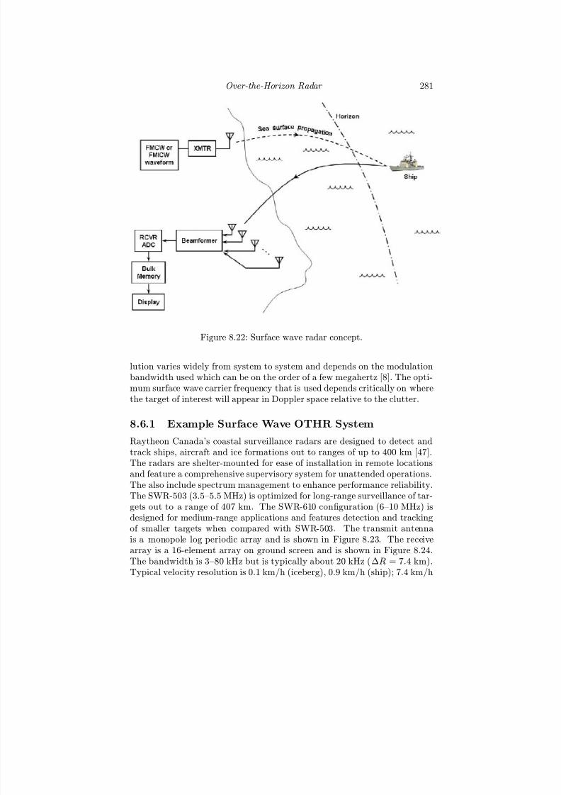
7/17/2019 1596932341 Intercept Radar.pdf
http://slidepdf.com/reader/full/1596932341-intercept-radarpdf 312/891
Over-the-Horizon Radar 281
Figure 8.22: Surface wave radar concept.
lution varies widely from system to system and depends on the modulationbandwidth used which can be on the order of a few megahertz [8]. The opti-mum surface wave carrier frequency that is used depends critically on wherethe target of interest will appear in Doppler space relative to the clutter.
8.6.1 Example Surface Wave OTHR System
Raytheon Canada’s coastal surveillance radars are designed to detect andtrack ships, aircraft and ice formations out to ranges of up to 400 km [47].The radars are shelter-mounted for ease of installation in remote locationsand feature a comprehensive supervisory system for unattended operations.The also include spectrum management to enhance performance reliability.The SWR-503 (3.5—5.5 MHz) is optimized for long-range surveillance of tar-gets out to a range of 407 km. The SWR-610 configuration (6—10 MHz) isdesigned for medium-range applications and features detection and trackingof smaller targets when compared with SWR-503. The transmit antennais a monopole log periodic array and is shown in Figure 8.23. The receivearray is a 16-element array on ground screen and is shown in Figure 8.24.The bandwidth is 3—80 kHz but is typically about 20 kHz (∆R = 7.4 km).Typical velocity resolution is 0.1 km/h (iceberg), 0.9 km/h (ship); 7.4 km/h

7/17/2019 1596932341 Intercept Radar.pdf
http://slidepdf.com/reader/full/1596932341-intercept-radarpdf 313/891
282 Detecting and Classifying LPI Radar
(aircraft). The average transmitter power is 3.2 kW with a peak power of 16 kW. The detection capability for the SWR-503 is shown in Figure 8.25 forseveral classes of air and surface targets.
Figure 8.23: SWR-503 transmit antenna configuration [47].
8.7 Surface Wave LPI Waveform
Considerations
There are two problems with FMCW for surface wave systems. First, thenecessary isolation between the transmitter and receiver for continuous-waveoperation at HF frequencies is more difficult to achieve. Second, due to thepropagation losses, the signal levels decrease rapidly with distance and thedynamic range of the signals exceeds that of any available receiver hardware[7]. Due to heavy user congestion, surface wave OTHR systems are alsorestricted to operating within narrow frequency bands.
8.7.1 FMICW Characteristics
To overcome these problems, the spectrum must be made discontinuous andFMICW type signals are used [48]. The FMICW is an FMCW waveform that
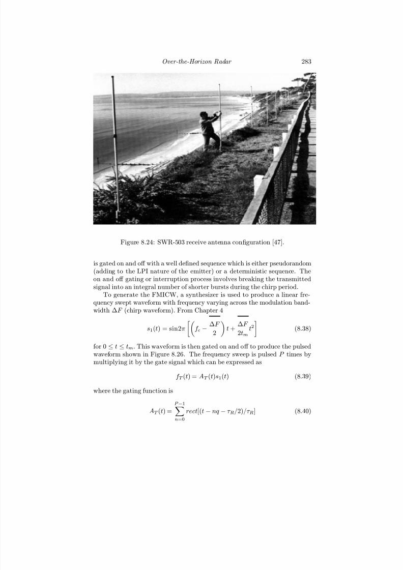
7/17/2019 1596932341 Intercept Radar.pdf
http://slidepdf.com/reader/full/1596932341-intercept-radarpdf 314/891
Over-the-Horizon Radar 283
Figure 8.24: SWR-503 receive antenna configuration [47].
is gated on and off with a well defined sequence which is either pseudorandom(adding to the LPI nature of the emitter) or a deterministic sequence. Theon and off gating or interruption process involves breaking the transmittedsignal into an integral number of shorter bursts during the chirp period.
To generate the FMICW, a synthesizer is used to produce a linear fre-quency swept waveform with frequency varying across the modulation band-width ∆F (chirp waveform). From Chapter 4
s1(t) = sin2π
f c −
∆F
2
t +
∆F
2tmt2
(8.38)
for 0 ≤ t ≤ tm. This waveform is then gated on and off to produce the pulsedwaveform shown in Figure 8.26. The frequency sweep is pulsed P times bymultiplying it by the gate signal which can be expressed as
f T (t) = AT (t)s1(t) (8.39)
where the gating function is
AT (t) =P −1n=0
rect[(t− nq − τ R/2)/τ R] (8.40)
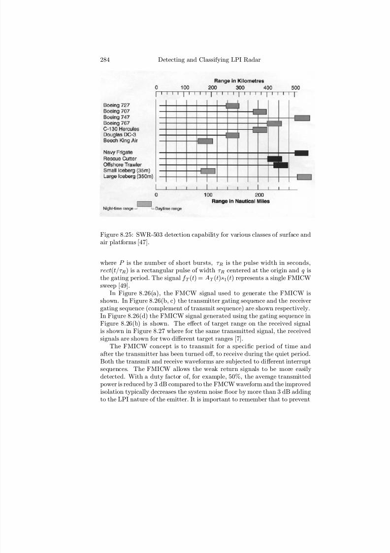
7/17/2019 1596932341 Intercept Radar.pdf
http://slidepdf.com/reader/full/1596932341-intercept-radarpdf 315/891
284 Detecting and Classifying LPI Radar
Figure 8.25: SWR-503 detection capability for various classes of surface andair platforms [47].
where P is the number of short bursts, τ R is the pulse width in seconds,rect(t/τ R) is a rectangular pulse of width τ R centered at the origin and q isthe gating period. The signal f T (t) = AT (t)s1(t) represents a single FMICWsweep [49].
In Figure 8.26(a), the FMCW signal used to generate the FMICW isshown. In Figure 8.26(b, c) the transmitter gating sequence and the receivergating sequence (complement of transmit sequence) are shown respectively.In Figure 8.26(d) the FMICW signal generated using the gating sequence inFigure 8.26(b) is shown. The eff ect of target range on the received signalis shown in Figure 8.27 where for the same transmitted signal, the receivedsignals are shown for two diff erent target ranges [7].
The FMICW concept is to transmit for a specific period of time andafter the transmitter has been turned off , to receive during the quiet period.Both the transmit and receive waveforms are subjected to diff erent interruptsequences. The FMICW allows the weak return signals to be more easilydetected. With a duty factor of, for example, 50%, the average transmitted
power is reduced by 3 dB compared to the FMCW waveform and the improvedisolation typically decreases the system noise floor by more than 3 dB addingto the LPI nature of the emitter. It is important to remember that to prevent

7/17/2019 1596932341 Intercept Radar.pdf
http://slidepdf.com/reader/full/1596932341-intercept-radarpdf 316/891
Over-the-Horizon Radar 285
Figure 8.26: (a—d) FMICW generation showing transmit and receive gating
(from [7]).
eclipsing, the receiver must always be off whenever the transmitter is on.Further diff erences between the two sequences are introduced by soft gating
which is used to suppress transients that would be caused if the interruptsequences were switched rapidly between on and off states [7].
The radar returns from the targets are delayed by the two-way travel timetd and are modified by the receiver gating sequence AR(t) as
f R(t) = AR(t)AT (t− td)s1(t− td) (8.41)
or
f R(t + td) = AR(t + td)AT (t)s1(t) (8.42)With the FMICW, the receiver must always be off whenever the transmitteris on so that the transmitter and receiver interrupt sequences are not identi-

7/17/2019 1596932341 Intercept Radar.pdf
http://slidepdf.com/reader/full/1596932341-intercept-radarpdf 317/891
286 Detecting and Classifying LPI Radar
Figure 8.27: FMICW radar echo from target with two-way travel time of (a) t1 s and (b) t2 s (from [7]).
cal. This interrupted spectrum gives rise to high-range side lobes and conse-quently a low dynamic range [50]. Diff erences between the two sequences areintroduced by the soft gating used to suppress these transients that wouldbe caused if the interrupt sequences were switched rapidly between the onand off states. Depending on the target’s range, the transmitted waveform isgenerally not received at the radar in its entirety.
There are three ways to extract the spectrum of the received echo fromthe target. The first method is to weight the return signal bursts individuallyand process the complete return as for a conventional FMCW receiver usinga single long FFT. The second method is to weight each burst individuallyand pack the remainder of the signal with zeros and process the completereturn as for a conventional FMCW receiver. The third method is to weighteach burst individually and process each short section using an FFT matchedto its length. Here an FFT with a duration equal to the burst period is usedto produce a spectrum. The number of floating point operations required

7/17/2019 1596932341 Intercept Radar.pdf
http://slidepdf.com/reader/full/1596932341-intercept-radarpdf 318/891

7/17/2019 1596932341 Intercept Radar.pdf
http://slidepdf.com/reader/full/1596932341-intercept-radarpdf 319/891
288 Detecting and Classifying LPI Radar
range bin samples to calculate the covariance matrix and correlation vector asdescribed in [15]. Improvements in signal-to-interference ratio on the orderof 20 dB can be achieved. The sparse waveform approach is to find theinterference-free channels in the HF band and then transmit the signal inthese clear channels. The main problem caused by the spectrum discontinuityis the range side lobes that are created [8]. Another interesting approach is touse a multiparametric generalization of the nonuniform FMICW train and byexploiting a factorization of the ACF based on genetic algorithms, an optimalsolution has been proposed [8].
A new FMICW waveform is presented in [51] and provides high-rangeresolution using a larger modulation bandwidth and a narrow modulationperiod to achieve a longer coherent integration time for high-speed targets.To prevent the high speed targets from smearing into many range cells duringthe longer integration periods, two frequency sweep bandwidths with diff er-ent sweep repetition intervals are used to determine the required coherent
integration time (CIT) and∆
R independently. The target velocities are esti-mated using one waveform and then applied to compensate the velocity phaseterms to account for the target movement. Due to the ability of higher ordercorrelation and spectral analysis methods to eff ectively suppress symmetricaldistributions such as Gaussian noise, these techniques have also been exploredfor interference cancelation and signal detection in OTHR [52].
8.8 Surface Wave Maximum Detection Range
The HF radar system planning and implementation problem is compoundedby the influence of the conducting ground plane on the radiation resistance of radar antennas and target backscattering cross-section. The potential errorresulting from basing a system design on a radar equation with an inconsistentset of parameter definitions is high. Without careful attention to detail,predicted received signal-to-noise ratios might be in error by 10 dB or more.
To determine the maximum detection range as a function of the inputrequired SNR, we develop the surface wave radar equation taking into accountthree eff ects that do not occur in conventional radars [53]:
1. A doubling of field strength due to direct and ground reflected waves;
2. A mutual impedance between the antennas and their images in theground plane;
3. A coupling between the target and its image in the ground plane.
Eff ects (2) and (3) are only significant when the antenna or the target is within
approximately one wavelength of the ground. Due to the HF wavelength,most antennas and some classes of target will be within one wavelength of the ground and so the eff ects cannot be ignored. The coupling of the antennas

7/17/2019 1596932341 Intercept Radar.pdf
http://slidepdf.com/reader/full/1596932341-intercept-radarpdf 320/891
Over-the-Horizon Radar 289
Table 8.1: RISP Gains for Some Example Antennas
Gain (dB)Antenna RISP dBiIsotropic in free-space 0 0Isotropic on a perfect ground plane 0 3Hertzian dipole in free-space 1.8 1.8Hertzian dipole on a perfect ground plane 1.8 4.8λ/4 monopole on a perfect ground plane 2.2 5.2
and target with their images in the ground modifies their radiation resistancesand this is the root cause of eff ects (2) and (3). In this section it is convenientto describe the gain of an antenna as Relative to an isotropic antenna at thesame position (RISP). The RISP gain of some example antennas are presentedin Table 8.1 along with the dBi value.
To develop the surface wave equation we follow the development in [53]and begin with the power flux F i, incident on a target due to transmissionfrom a vertical Hertzian dipole over a perfectly conducting ground plane
F i = E 2
Z 0=
ptgt [2sin θ cos(kht cos θ)]2
4πd2(1 + ∆t) (8.44)
where E is the field strength, Z 0 the impedance of free-space, pt the radiatedpower in the presence of the ground, the transmitting antenna has RISP gaingt and d is the distance between transmitter and target. The term (1+∆t) is afactor to allow for coupling between the antenna and its image in the ground.The angle θ is the zenith angle of the target measured at the transmitter,k = 2π/λ, and ht is the dipole height above the ground. The term ∆ is givenby
∆ =
3(2kh)2
sin(2kh)
2kh − cos(2kh)
(8.45)
At h = 0, (1 +∆) = 2. For h > λ, (1 + ∆) ≈ 1. The term in square bracketsin (8.44) gives the vector sum of direct and ground reflected signals. Whenθ → π/2
F i = ptgt
4πd2(1 + ∆t)4 (8.46)
The trailing factor of 4 is due to the in-phase addition of the direct andground-reflected waves.
For the collecting aperture of a target consider that the target is a matchedantenna with RISP gain gx. The power available to the matched load is equalto that which is reradiated. The target power collecting aperture is given by
gxλ24π
· 1(1 + ∆x)
(8.47)
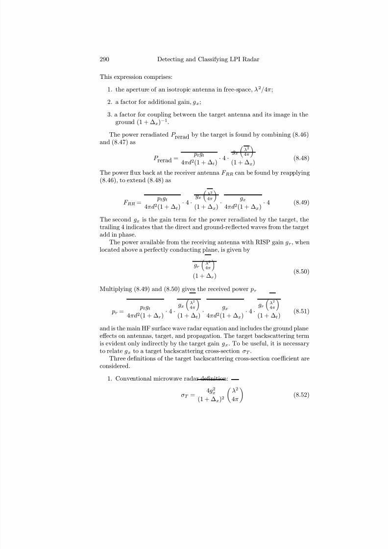
7/17/2019 1596932341 Intercept Radar.pdf
http://slidepdf.com/reader/full/1596932341-intercept-radarpdf 321/891
290 Detecting and Classifying LPI Radar
This expression comprises:
1. the aperture of an isotropic antenna in free-space, λ2/4π;
2. a factor for additional gain, gx;
3. a factor for coupling between the target antenna and its image in theground (1 +∆x)−1.
The power reradiated P rerad by the target is found by combining (8.46)and (8.47) as
P rerad = ptgt
4πd2(1 + ∆t) · 4 ·
gx
λ2
4π
(1 + ∆x)
(8.48)
The power flux back at the receiver antenna F RR can be found by reapplying(8.46), to extend (8.48) as
F RR = ptgt
4πd2(1 + ∆t) · 4 ·
gxλ2
4π
(1 + ∆x)
· gx
4πd2(1 + ∆x) · 4 (8.49)
The second gx is the gain term for the power reradiated by the target, thetrailing 4 indicates that the direct and ground-reflected waves from the targetadd in phase.
The power available from the receiving antenna with RISP gain gr, whenlocated above a perfectly conducting plane, is given by
gr
λ2
4π
(1 + ∆r)
(8.50)
Multiplying (8.49) and (8.50) gives the received power pr
pr = ptgt
4πd2(1 + ∆r) · 4 ·
gxλ2
4π
(1 + ∆t)
· gx
4πd2(1 + ∆x) · 4 ·
grλ2
4π
(1 + ∆t)
(8.51)
and is the main HF surface wave radar equation and includes the ground planeeff ects on antennas, target, and propagation. The target backscattering termis evident only indirectly by the target gain gx. To be useful, it is necessaryto relate gx to a target backscattering cross-section σT .
Three definitions of the target backscattering cross-section coefficient areconsidered.
1. Conventional microwave radar definition:
σT = 4g2x
(1 + ∆x)2
λ2
4π
(8.52)

7/17/2019 1596932341 Intercept Radar.pdf
http://slidepdf.com/reader/full/1596932341-intercept-radarpdf 322/891
Over-the-Horizon Radar 291
and relates the scattering cross-section of a matched antenna of RISPgain gx above a perfectly conducting ground plane with elevation h > λ.The factor (1 + ∆x)−2 accounts for the antenna collecting and reradi-ating properties.
2. Free-space backscattering cross-section definition:
σFS = g2x
λ2
4π
(8.53)
and relates the backscattering cross-section of an isotropic antenna infree-space (absence of a ground plane). If the isotropic antenna werereplaced by a target antenna with RISP gain gx, then its backscatteringcross-section in free-space is given by σFS .
3. Shearman’s definition [54]:
σs =g2xλ
2
4π
(1 + ∆x)2 (8.54)
which departs from the conventional microwave radar definition by afactor of 4 to allow for the ground reflection on the signal’s return tothe receiver.
By substituting for gx from (8.52), (8.53), and (8.54) into (8.49), we obtainthree diff erent equations, all equally valid, but using diff erent definitions of the target cross-section:
pr = ptgt
4πd2(1 + ∆t) · 4 ·
λ2
4π
(1 + ∆x)
· σT (1 + ∆x)2
4 λ24π (8.55)
· 1
4πd2(1 + ∆x) · 4 ·
grλ2
4π
(1 + ∆r)
pr = ptgt
4πd2(1 + ∆t) · 4 ·
λ2
4π
(1 + ∆x)
· σFS λ2
4π
(8.56)
· 1
4πd2(1 + ∆x) · 4 ·
gr
λ2
4π
(1 + ∆r)
pr = ptgt
4πd2(1 + ∆t) · 4 ·
λ2
4π
(1 + ∆x)
· σs(1 + ∆x)2
λ2
4π (8.57)
· 1
4πd2(1 + ∆x) · 4 ·
grλ
2
4π
(1 + ∆r)
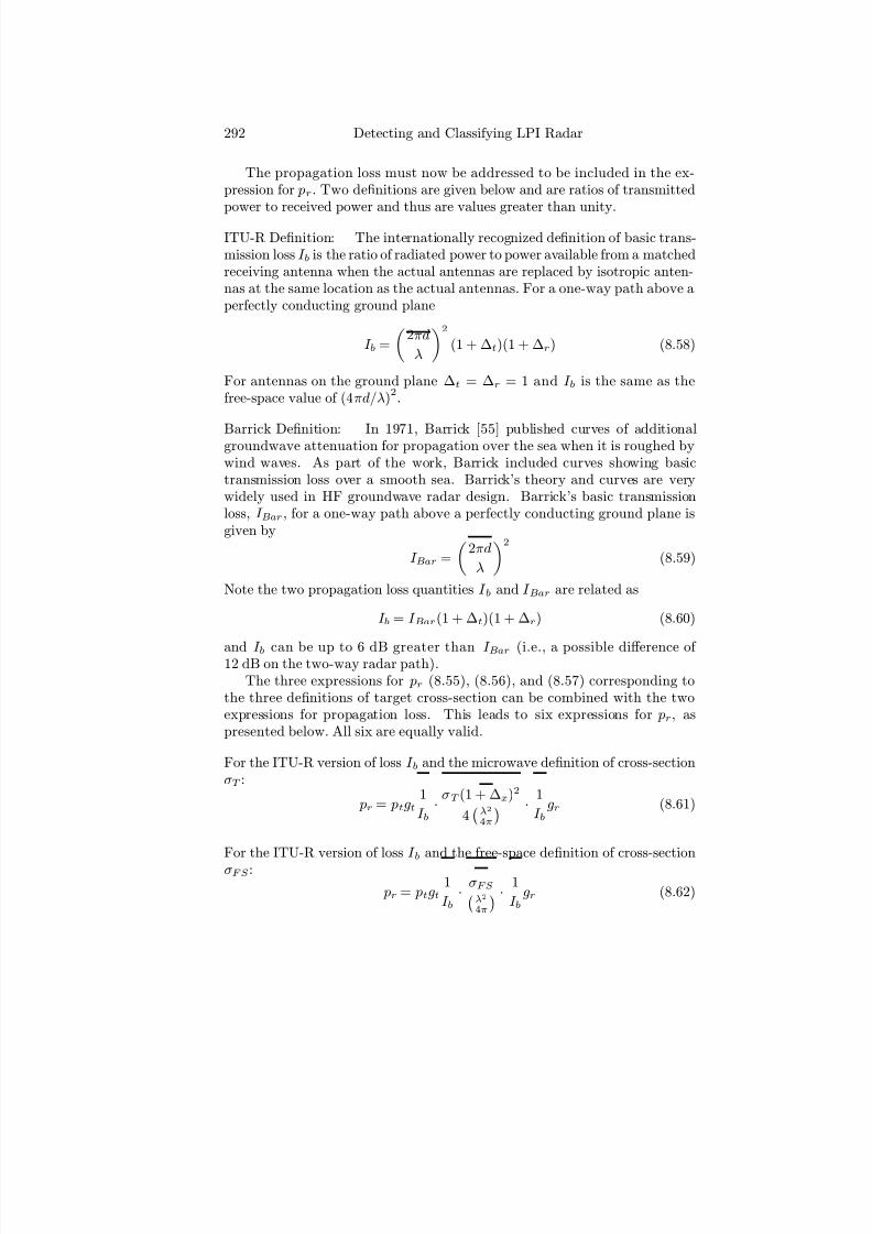
7/17/2019 1596932341 Intercept Radar.pdf
http://slidepdf.com/reader/full/1596932341-intercept-radarpdf 323/891
292 Detecting and Classifying LPI Radar
The propagation loss must now be addressed to be included in the ex-pression for pr. Two definitions are given below and are ratios of transmittedpower to received power and thus are values greater than unity.
ITU-R Definition: The internationally recognized definition of basic trans-mission loss I b is the ratio of radiated power to power available from a matchedreceiving antenna when the actual antennas are replaced by isotropic anten-nas at the same location as the actual antennas. For a one-way path above aperfectly conducting ground plane
I b =
2πd
λ
2
(1 + ∆t)(1 + ∆r) (8.58)
For antennas on the ground plane ∆t = ∆r = 1 and I b is the same as thefree-space value of (4πd/λ)
2.
Barrick Definition: In 1971, Barrick [55] published curves of additionalgroundwave attenuation for propagation over the sea when it is roughed bywind waves. As part of the work, Barrick included curves showing basictransmission loss over a smooth sea. Barrick’s theory and curves are verywidely used in HF groundwave radar design. Barrick’s basic transmissionloss, I Bar , for a one-way path above a perfectly conducting ground plane isgiven by
I Bar =
2πd
λ
2
(8.59)
Note the two propagation loss quantities I b and I Bar are related as
I b = I Bar(1 + ∆t)(1 + ∆r) (8.60)
and I b can be up to 6 dB greater than I Bar (i.e., a possible diff erence of 12 dB on the two-way radar path).
The three expressions for pr (8.55), (8.56), and (8.57) corresponding tothe three definitions of target cross-section can be combined with the twoexpressions for propagation loss. This leads to six expressions for pr, aspresented below. All six are equally valid.
For the ITU-R version of loss I b and the microwave definition of cross-sectionσT :
pr = ptgt1
I b· σT (1 + ∆x)2
4λ2
4π
· 1
I bgr (8.61)
For the ITU-R version of loss I b and the free-space definition of cross-section
σFS :
pr = ptgt1
I b· σFS λ2
4π
· 1
I bgr (8.62)

7/17/2019 1596932341 Intercept Radar.pdf
http://slidepdf.com/reader/full/1596932341-intercept-radarpdf 324/891
Over-the-Horizon Radar 293
For the ITU-R version of loss I b and the Shearman definition of cross-sectionσs:
pr = ptgt1
I b · σs(1 + ∆x)2)
λ2
4π
·
1
I b gr (8.63)
For the Barrick version of loss I Bar and the microwave definition of cross-section σT :
pr = ptgt1
I Bar(1 + ∆t)(1 + ∆x) · σT (1 + ∆x)2
4λ2
4π
(8.64)
· 1
I Bar(1 + ∆r)(1 + ∆x) · gr
For the Barrick version of loss I Bar and the free-space definition of cross-
section σFS :
pr = ptgt1
I Bar(1 + ∆t)(1 + ∆x) · σFS λ2
4π
· 1
I Bar(1 + ∆r)(1 + ∆x) · gr (8.65)
For the Barrick version of loss I Bar and the Shearman definition of cross-section σs:
pr = ptgt1
I Bar(1 + ∆t)(1 + ∆x) · σs(1 + ∆x)2
λ2
4π
(8.66)
· 1
I Bar(1 + ∆r)(1 + ∆x) · gr
The maximum detection range of the surface wave emitter can be deter-mined by substituting the receiver’s sensitivity
δ I = kT 0F RBRi(SNRRi) (8.67)
for the return power pr (given by the six equations) and then solving for thedistance d. Figure 8.28 shows the results of two simulations (f c = 5 MHz andf c = 15 MHz) using the surface wave MATLAB code surface detect.m on theCD. Other (default) parameters include pt = 100 kW, gt = gr = gx3 dB,ht = hr = 10m, hx = 5m. The emitter input bandwidth BRi = 30 MHz andthe receiver has a noise factor of F R = 10 dB with kT 0 = 4 × 10⁻²¹ W/Hz.
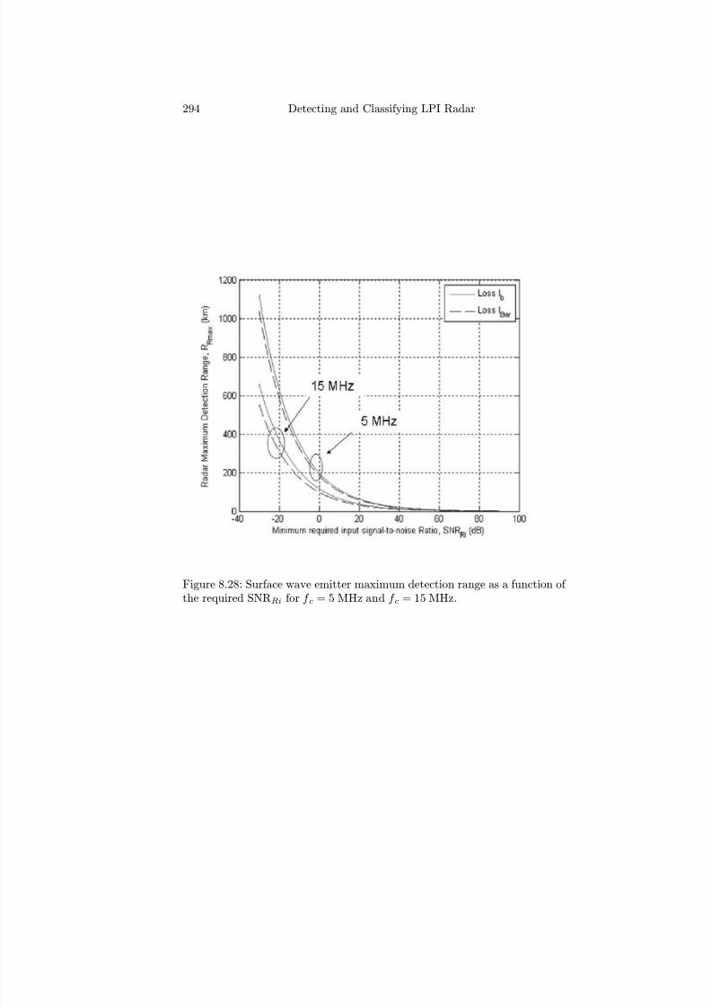
7/17/2019 1596932341 Intercept Radar.pdf
http://slidepdf.com/reader/full/1596932341-intercept-radarpdf 325/891
294 Detecting and Classifying LPI Radar
Figure 8.28: Surface wave emitter maximum detection range as a function of the required SNRRi for f c = 5 MHz and f c = 15 MHz.

7/17/2019 1596932341 Intercept Radar.pdf
http://slidepdf.com/reader/full/1596932341-intercept-radarpdf 326/891
Over-the-Horizon Radar 295
8.9 Concluding Remarks
Both surface wave and sky wave radars experience ionospheric clutter (un-
wanted backscatter from the moving ionosphere) that can sometimes hidethe presence of the desired target echoes. Sky wave radars can also suf-fer significant polarization losses and focusing/defocusing problems due toionospheric eff ects. Military HF radars are susceptible to deliberate jammingand consequently they are incorporating LPI waveforms and techniques toprevent their detection while fulfilling their early warning role while avoidingelectronic warfare measures (for example, see [4, 15]).
Another significant problem in OTHR is robust high-resolution Dopplerprocessing of accelerating or decelerating targets. The ionosphere often mod-ulates the return signals and spreads the Doppler, which makes it difficultto detect targets. This Doppler eff ect arises during aircraft and ship targetmaneuvers and during observations of rockets in boost phase and mid-coursephase flight. Most OTHR systems use classical Doppler processing, whereone Doppler spectrum is computed using one full CIT. Typically, the CIT ison the order of 1—100 seconds in OTHR systems. Some systems use over-lapped Doppler processing to provide a spectrogram analysis of time-varyingDoppler [6].
Today, more than ever, the prediction of OTHR performance is importantespecially for naval systems that are trying to avoid being detected at a long-range distance. Sky wave simulation results show that for Rfootprint = 3500
km, the minimum required input SNR (SNRRi) for f c = 14.5 MHz for σT =1, 10, and 100 m2 is −107, −97 and −87 dB, respectively, from Figure 8.16.PROPLAB results have been shown for one day. The results however willchange depending on the time of year as well as the time of day.
References
[1] Wise, J.C., “Summary of Recent Australian Radar Developments,” IEEE
Aerospace and Electronic Systems Magazine , pp. 8—10, Dec. 2004.
[2] Kolosov, A. A., Over-the-Horizon Radar , Artech House Inc., Norwood, MA,1987.
[3] Headrick, J. M., and Skolnik, M. I., “Over-the-horizon radar in the HF band,”Proc. of IEEE , Vol. 62, No. 6, pp. 664—673, 1974.
[4] Green, S. D., Kingsley, S. P., and Biddiscombe, J. A., “HF radar waveformdesign,” Proceedings of the HF Radio Systems and Techniques Conf., 4—7July, pp. 202—206, 1994.
[5] Musa, M., and Salous, S., “Ambiguity elimination in HF FMCW radar sys-
tems,” IEE Proc. Radar, Sonar and Navig. Vol. 147, No. 4, pp. 182—188,Aug. 2000.
7/17/2019 1596932341 Intercept Radar.pdf
http://slidepdf.com/reader/full/1596932341-intercept-radarpdf 327/891
296 Detecting and Classifying LPI Radar
[6] Musa, M., and Salous, S., “Evaluation of multiple WRF-HF-FMCW radarwaveforms,” Proc. of the IEE HF Radio Systems and Techniques Conf., pp.207—211, 2000.
[7] Khan, R. H., and Mitchell, D. K., “Waveform analysis for high-frequencyFMICW radar,” IEE Proc.-F , Vol. 138, No. 5, pp. 411—419, Oct. 1991.
[8] Liu, W. X., Lu, Y. L., and Lesturgie, M., “Optimal sparse waveform designfor HFSWR system,” International Waveform Diversity and Design Conf.,pp. 127—130, 4—8 June 2007.
[9] Guo, X., Ni, J. L., Liu, G. S., “Ship detection with short coherent integrationtime in over-the-horizon radar,” Proc. of the International Conf. on Radar ,pp. 667—671, 3—5 Sept. 2003.
[10] Anderson, S. J., Mei, F. J., and Peinan, J., “Enhanced OTHR ship detectionvia dual frequency operation,” Proc. of the CIE International Conf. of Radar ,pp. 85—89, 2001.
[11] Wei, Y., and Liu, Y., “New anti-jamming waveform designing and processing
for HF radar,” Proceedings of CIE International Conf. of Radar , pp. 281—284,2001.
[12] Frazer, G. J., Abramovich, Y. I., and Johnson, B. A., “Spatially waveformdiverse radar: perspectives for high frequency OTHR,” Proc. of the IEEE
Radar Conf., pp. 385—390, 2007.
[13] Topliss, R. J., Maclean, A. B., Wade, S. H., Wright, P. G., and Parry, J. L.,“Reduction of interference by high power HF radar transmitters,” Proc. of
the IEE HF Radio Systems and Techniques Conf., No. 411, pp. 251—255,July 1997.
[14] Turley, M. D. E., “FMCW radar waveforms in the HF band,” Input to theITU-R JRG 1A-1C-8B meeting, November 2006.http://www.its.bldrdoc.gov/meetings/itu-r/contributions4/jrg-73.pdf.
[15] Xianrong, W., Hengyu, K., and Biyang, W., “Adaptive cochannel interferencesuppression based on subarrays for HFSWR,” IEEE Signal Processing Letters ,Vol. 12, No. 2, pp. 162—165, Feb. 2005.
[16] Lu, K., Liu, X., and Liu, Y., “Ionospheric decontamination and sea cluttersuppression for HF skywave radars,” IEEE Journal of Oceanic Engineering ,Vol. 30, No. 2, pp. 455—462, April 2005.
[17] Guo, X., Hongbo, S., and Yeo, T. S., “Transient interference excision in over-the-horizon radar using adaptive time-frequency analysis,” IEEE Trans. on
Geoscience and Remote Sensing , Vol. 43, No. 4, pp. 722—735, April 2005.
[18] Tarran, C. J., “Operational HF DF systems employing real time superresolu-tion processing,” Proc. of the IEE HF Radio Systems and Techniques Conf.,No. 411, pp. 311—319, July 1997.
[19] Dawber, W. N., Pote, M. F., Turner, S. D., Graddon, J. M., Barker, D.,
Evans, G., and Wood, S. G., “Integrated antenna architecture for high fre-quency multifunction naval systems,” Proc. of the CIE International Conf.
of Radar , pp. 1—5, 2006.

7/17/2019 1596932341 Intercept Radar.pdf
http://slidepdf.com/reader/full/1596932341-intercept-radarpdf 328/891
Over-the-Horizon Radar 297
[20] Huang, G., Meng, J., and Yang, L., “Time-delay estimation for sub-samplingsinusoidal signals,” Proc. of the International Conf. on Communications,
Circuits and Systems , pp. 761—764, 2005.
[21] Xiaodong, T., Yunjie, H., and Wenyu, Z., “Sky wave over-the-horizon backscat-ter radar,” Proceedings of the CIE International Conf. on Radar , pp. 90—94,15—18 Oct. 2001.
[22] Liu, B-Y, Pace, P. E., and Knorr, J. B., “HF skywave FMCW OTH-B systemsexpected emitter footprint,” Proc. of the IEEE System of Systems Engineer-
ing Conf., Monterey, CA, June 2008.
[23] Kingsley, S., and Quegan, S., Understanding Radar Systems , Scitech, Mend-ham, NJ, 1999.
[24] Davies, K., Ionospheric Radio, IEE Electromagnetic Waves Series, Vol. 31,IEEE Electromagnetic Waves Series, 1990.
[25] http://www.utdallas.edu/research/spacesciences/ionosphere.htm(The Earth’s Ionosphere).
[26] Dyson, P. L., and Bennett, J. A., “Exact ray path calculations using realisticionospheres,” IEE Proc. - H , Vol. 139, No. 5, pp. 407—413, Oct. 1992.
[27] Ong, C. Y., Bennett, J. A., and Dyson, P. L., “An improved method of synthesizing ground backscatter ionograms for spherical ionospheres,” Radio
Science , Vol. 33, No. 4, pp. 1173—1185, 1998.
[28] Croft, T. A., and Hoogasian, H., “Exact ray calculations in a quasi-parabolicionosphere with no magnetic field,” Radio Science, Vol. 3, No. 1, pp. 69—74,Jan. 1968.
[29] http://nssdc.gsfc.nasa.gov/nssdc news/june01/iri.html Ionospheric Model(IRI-2001).
[30] http://modelweb.gsfc.nasa.gov/models/iri.html IRI Model, Space PhysicsData Facility (SPDF).
[31] Jordan, E. C., and Balmain, K. G., Electromagnetic Waves and Radiating Systems , Prentice Hall, Inc., Englewood Cliff s, NJ, 1968.
[32] Barnes, R. J., “Automated propagation advice for OTHR ship detection,”IEE Proc. — Radar, Sonar, Navig., Vol. 143, No. 1, pp. 53—63, Feb. 1996.
[33] Gill, E. W., Howell, R. K., Hickey, K., Walsh, J. and Dawe, B. J., “High fre-quency ground wave radar measurement of ocean surface parameters duringthe ERS-1 calibration-validation experiment,” Proc. of OCEANS ’93 Engi-
neering in Harmony with Ocean , pp. I55—I60, 18—21 Oct. 1993.
[34] Georges, T. M., and Harlan, J. A., “New horizons for over-the-horizon radar,”IEEE Antennas and Propagation Magazine , Vol. 36, No. 4, pp. 14—24, Aug.1994.
[35] Jindalee Operational Radar Network (JORN), Jane’s Radar and ElectronicWarfare Systems, Land-Based Air Defence Radars, January 10, 2007.
[36] Gurgel, K-W, Essen, H-H, Schlick, T., “HF surface wave radar for oceanography—a review of activities in Germany,” Proc. of the International Radar Conf.,pp. 700—705, 2003.

7/17/2019 1596932341 Intercept Radar.pdf
http://slidepdf.com/reader/full/1596932341-intercept-radarpdf 329/891
298 Detecting and Classifying LPI Radar
[37] Hartnett, M. P. and Clancy J. T., “Utilization of a nonrecurrent waveform tomitigate range-folded spread Doppler clutter: Application to over-the-horizonradar,” Radio Science Vol. 33, No. 4, pp. 1125—1133, 1998.
[38] Zhang, Y., Amin, M. G. Amin and Frazer, G. J., “High-resolution time-frequency distributions for manoeuvring target detection in over-the-horizonradars,” IEE Proc. — Radar Sonar Navig., Vol. 150, No. 4, pp. 299—304,Aug. 2003.
[39] Pace, P. E., Advanced Techniques for Digital Receivers , Artech House Inc.,Norwood, MA, 2000.
[40] “Chinese OTH Radar,” Jane’s C4I Systems, Intelligence Systems in Direction
Finding , June, 2000.
[41] Li, N.-J., “A review of Chinese designed surveillance radars—past, presentand future,” Record of the IEEE International Radar Conf., pp. 288—293,Alexandria, VA, May 8-11, 1995.
[42] Krolik, J. L., Anderson, R. H., “Maximum likelihood coordinate registration
for over-the horizon radar,” IEEE Trans. on Signal Processing, Vol. 45, No.4, pp. 945—959, April 1997.
[43] Torrez, W. C., and Blasch, E., “An application of generalized least squaresbias estimation for over-the-horizon radar coordinate registration,” Proc. of
the Third International Conf. on Information Fusion , Volume 1, 10—13 July,2000.
[44] Min, K., Wang, G-H, and Wang, X-B, “Coordinates registration and erroranalysis based on spherical model for OTH radar,” Proc. of the International
Conf. on Radar , pp. 1—4, Oct. 2006.
[45] PROPLAB-PRO version 2.0 User’s Manual, High Frequency Radio ProgramLaboratory, 1994-1997.
[46] http://areps.spawar.navy.mil/AREPS (Advanced Refractive Eff ects Prediction System)
[47] SWR series High-Frequency Surface Wave Radars (HFSWR), Naval/CoastalSurveillance and Navigation Radars, Canada, Jane’s Radar And Electronic
Warfare Systems , April 10, 2007.
[48] Yang, S., Ke, H., Wu, X., Tian, J., and Hou, J., “HF radar ocean currentalgorithm based on MUSIC and the validation experiments,” IEEE Journal
of Oceanic Engineering , Vol. 30, No. 3, pp. 601—618, July 2005.
[49] Kahn, R., Gamberg, B., Power, D., Walsh, J., Dawe, B., Pearson, W., andMillan, D., “Target detection and tracking with a high frequency ground waveradar,” IEEE Journal of Oceanic Engineering, Vol. 19, No. 4, pp. 540—548,Oct. 1994.
[50] Green, S. D., and Kingsley, S. P., “Improving the range/time sidelobes of large bandwidth discontinuous spectra HF radar waveforms,” Proc. of the
IEE HF Radio Systems and Techniques , No. 411 00. 246—250, July 1997.
[51] Yiying, S., Ning, Z., and Yongtan, L., “New waveform with both high rangeresolution and long coherent integration time in a HF radar,” Proceedings of
CIE International Conf. of Radar , pp. 285—288, 8—10 Oct. 1996.
7/17/2019 1596932341 Intercept Radar.pdf
http://slidepdf.com/reader/full/1596932341-intercept-radarpdf 330/891
Over-the-Horizon Radar 299
[52] Zongchuang, L., Zingzhao, L., and Yongtan, L., “A signal detection algorithmbased on higher-order statistics for HFSW-OTH radar,” Proceedings of CIE
International Conf. of Radar , pp. 996—1000, 2001.
[53] Milsom, J. D., “HF groundwave radar equations,” Proc. of the IEE HF Radio
Systems and Techniques , No. 411, pp. 285—290, July 1997.
[54] Barrick, D. E., “First order theory and analysis of MF/HF/VHF scatter fromthe sea,” IEEE Trans. on Antennas and Propagation , AP-20, pp. 2—10, 1972.
[55] Barrick, D. E., “Theory of HF and VHF propagation across the rough sea,”Parts I and II, Radio Science Vol. 6, No. 5, pp. 517—533, 1971.
Problems
1. A target’s range is measured with a t0 = 200 ms and shows up in rangebin 15. If the target has a Doppler shift of 20 Hz, what is the corrected
range bin of the target?2. Wideband clutter covers 200—500 km. If a FMCW waveform with
∆F = 10 kHz is used, in what range bins will the clutter appear?
3. In the multiple WRF technique, if the ∆F = 10 kHz and if the num-ber of range bins covered by the clutter is N RB = 40 (a) what is themaximum integer value for WRF2? and (b) what are the three WRFs?
4. Consider a multiple WRF FMCW radar with a bandwidth∆F = 20 kHz and WRF1 = 7 Hz, WRF2 = 8 Hz, and WRF3 = 9 Hzand an integration time of 150s (each block is 50s). For the first block(WRF1), determine (a) the total number of range bins, (b) the rangeresolution, and (c) the corresponding maximum unambiguous range.
(d) Repeat (a)—(c) for WRF2 and WRF3. (e) What is the maximumclutter width (in km) in order that sea echoes and other unambiguoustargets can be detected?

7/17/2019 1596932341 Intercept Radar.pdf
http://slidepdf.com/reader/full/1596932341-intercept-radarpdf 331/891
7/17/2019 1596932341 Intercept Radar.pdf
http://slidepdf.com/reader/full/1596932341-intercept-radarpdf 332/891
Chapter 9
Case Study: Antiship LPI
Missile Seeker
In Chapter 1 we examined the characteristics that make a radar LPI, and inChapter 2 we looked at a number of important applications. A significantadvantage can be gained over the noncooperative intercept receiver when theradar uses frequency, phase, and hybrid wideband waveform coding tech-niques. In Chapter 3 the periodic ambiguity function was presented as ameans of quantifying the characteristics of the LPI waveforms, which are dis-cussed in Chapters 4—8. In this chapter, we bring some of these conceptstogether in a case study that examines the detection capability of a power-managed LPI antiship cruise missile seeker. In the scenario examined, theASCM has an FMCW seeker that attempts to detect and track a low radarcross section ship at the horizon. RCS values considered include 50, 100, and500 m2. To predict the target detection capability, sea clutter models aredeveloped, and the emitter is flown at 300 m/s in a scenario that starts at arange of 28 km from the target. Each sea state (0—4) is characterized by asecond-order polynomial that describes the normalized mean sea backscattercoefficient as a function of the grazing angle. The emitter transmit powerlevel is adapted to be consistent with the RCS and range to the target, whilekeeping the output signal to noise ratio SNRRo at 20 dB. A brief history of ASCM seeker technology is given first.
9.1 History of ASCM Seeker Technology
Antiship cruise missiles have been a significant threat to navy surface shipsfor many years. The first generation of ASCM threats (prior to 1969) used asingle-frequency RF pulse with a constant pulse repetition interval [1]. The
301
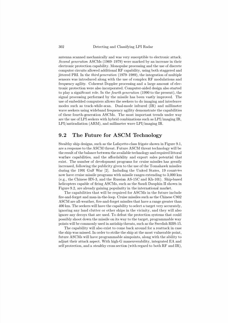
7/17/2019 1596932341 Intercept Radar.pdf
http://slidepdf.com/reader/full/1596932341-intercept-radarpdf 333/891
302 Detecting and Classifying LPI Radar
antenna scanned mechanically and was very susceptible to electronic attack.Second generation ASCMs (1969—1979) were marked by an increase in theirelectronic protection capability. Monopulse processing and the use of discretecomputer circuits allowed additional RF capability, using both staggered and
jittered PRI. In the third generation (1979—1989), the integration of multiplesensors was introduced along with the use of complex RF modulations andfrequency agility. Coherent Doppler processing and a large amount of elec-tronic protection were also incorporated. Computer-aided design also startedto play a significant role. In the fourth generation (1990 to the present), thesignal processing performed by the missile has been vastly improved. Theuse of embedded computers allows the seekers to do imaging and interleavemodes such as track-while-scan. Dual-mode infrared (IR) and millimeterwave seekers using wideband frequency agility demonstrate the capabilitiesof these fourth-generation ASCMs. The most important trends under wayare the use of LPI seekers with hybrid combinations such as LPI/imaging IR,LPI/antiradiation (ARM), and millimeter wave LPI/imaging IR.
9.2 The Future for ASCM Technology
Stealthy ship designs, such as the Lafayette-class frigate shown in Figure 9.1,are a response to the ASCM threat. Future ASCM threat technology will bethe result of the balance between the available technology and required littoralwarfare capabilities, and the aff ordability and export sales potential thatexist. The number of development programs for cruise missiles has greatlyincreased, following the publicity given to the use of the Tomahawk missiles
during the 1991 Gulf War [2]. Including the United States, 19 countriesnow have cruise missile programs with missile ranges extending to 3,000 km(e.g., the Chinese HN-3, and the Russian AS-15C and Kh-101). Ship-basedhelicopters capable of firing ASCMs, such as the Saudi Dauphin II shown inFigure 9.2, are already gaining popularity in the international market.
The capabilities that will be required for ASCMs in the future includefire-and-forget and man-in-the-loop. Cruise missiles such as the Chinese C802ASCM are all-weather, fire-and-forget missiles that have a range greater than400 km. The seekers will have the capability to select a target very accurately,ignoring any land clutter or other ships in the vicinity, and they will alsoignore any decoys that are used. To defeat the protection systems that couldpossibly shoot down the missile on its way to the target, programmable waypoints will be commonly used in antiship threats, such as the Swedish RBS-15.
The capability will also exist to come back around for a reattack in casethe ship was missed. In order to strike the ship at the most vulnerable point,future ASCMs will have programmable aimpoints, along with the ability toadjust their attack aspect. With high-G maneuverability, integrated EA andself protection, and a stealthy cross section (with regard to both RF and IR),
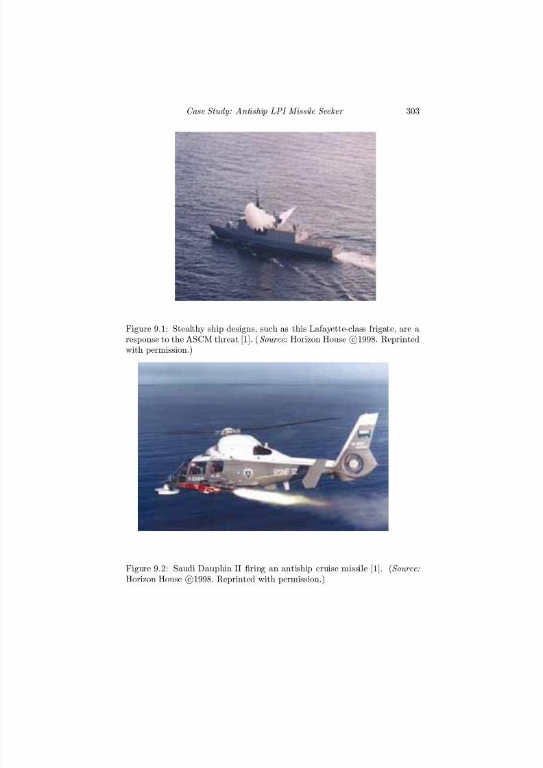
7/17/2019 1596932341 Intercept Radar.pdf
http://slidepdf.com/reader/full/1596932341-intercept-radarpdf 334/891
Case Study: Antiship LPI Missile Seeker 303
Figure 9.1: Stealthy ship designs, such as this Lafayette-class frigate, are aresponse to the ASCM threat [1]. (Source: Horizon House c1998. Reprintedwith permission.)
Figure 9.2: Saudi Dauphin II firing an antiship cruise missile [1]. (Source:
Horizon House c1998. Reprinted with permission.)

7/17/2019 1596932341 Intercept Radar.pdf
http://slidepdf.com/reader/full/1596932341-intercept-radarpdf 335/891
304 Detecting and Classifying LPI Radar
the future ASCM penetration capability will be ominous. The capability toperform coordinated salvos (coordination of multiple launch platforms) withsimultaneous arrival times will also increase the probability of hitting theship. Several ASCMs approaching a ship from multiple aspects coordinatedas a stream raid seem to make the odds of ship survival remote at best.
A number of advanced electronic technologies such as field-programmablegate arrays in GaAs, and application-specific integrated circuits, will be usedin future ASCMs. Low-probability-of-intercept, power-managed seekers op-erating in the 8- to 20-GHz range, as well as the 35- and 96-GHz ranges willuse pulse-to-pulse spread-spectrum modulation with coherent range Dopplerprocessing to target the ships. Phased arrays and active arrays will refine thetargeting capability, allowing variable sectors to be scanned using multiplebeams. Exclusion zones will also provide the ability to reject any decoys thatmight interfere with the target kill. The active seekers will also use othersophisticated modes, such as Doppler beam sharpening, unfocused syntheticaperture radar, and inverse synthetic aperture radar. Wideband ARM seekerswith phased arrays will be able to easily recognize and discriminate targets,and will be especially robust against emissions control tactics (RF < −110dBm). When faced with emissions-control tactics, these ARM seekers willalso use a technique called loitering, in which a parachute is deployed to slowthe missile until the radiation source comes back up.
Although not as prevalent today as RF seekers, infrared seekers are fastbecoming a force to be reckoned with. By 2010, large-scale InSb, HgCdTe,and PtSi imaging arrays on the order of 1,024 × 1,024 will be available. Newcooling techniques and the development of detectors that do not require cool-
ing will improve the fi
delity of the IR images. Improvements in IR domematerials, and protection against laser jammers and interrogators, will allowthe seeker to be very robust in the terminal phase of attack. Future dual-modetechnologies that will appear include ARM/millimeter-wave and ARM/laserradar using high-accuracy inertial systems for the terminal phase. For flightguidance, most new missiles are using an inertial navigation system (INS)together with global positioning system updates. Whereas a modern INS willhave an accuracy of about 2 km per flight hour at around Mach 0.85, a com-bined INS/GPS would have an accuracy of around 50 to 100m circular errorprobable (CEP)1 regardless of flight time. The use of fiber optics (instead of copper wire) will also make the weapon lighter and increase the range that itcan travel.
The RBS-15 shown in Figure 9.3 is an example of an advanced missile
1A circular error probable is determined by a series of flight tests, and is usually cal-culated by taking the square root of the sum of the squares of the range and track errors.The resultant CEP indicates the radius of the circle that encompasses half the impactpoints during the flight tests. The other half of the results could spread out to manytimes the CEP radius, and the CEP may be diff erent for diff erent ranges, flight profiles ortarget sets [2].

7/17/2019 1596932341 Intercept Radar.pdf
http://slidepdf.com/reader/full/1596932341-intercept-radarpdf 336/891
Case Study: Antiship LPI Missile Seeker 305
Figure 9.3: Swedish RBS-15 ASCM in flight [3] ( c2002 Jane’s InformationGroup).
that is designed to operate in all surface attack roles, from littoral warfare to
blue-water situations, and includes a day-and-night, all-weather, land-attackcapability. Its long range (over 200 km) and flexible trajectory mean thatit can attack hostile vessels well beyond the horizon, but also at very closeranges. The missiles, each individually prepared in a salvo, can be prepro-grammed to enable attacks to be mounted from diff erent directions, with apreselected time of arrival for each missile to confuse air defenses. Using anadvanced missile engagement planning system, the missiles can make use of terrain masking for a concealed approach, to minimize warning time.
9.3 Detecting the Threat
To adequately defend the ship, the ASCM must be detected before it comes
over the horizon. The detection of an incoming cruise missile seeker at thehorizon (≈ 24 km) is difficult with modern ES intercept receivers. Since themissile usually flies just above the water surface, it is hard to detect andextract it from the clutter using radar, since the RCS can be very small. TheASCM is also hard to detect with infrared sensors. It can possibly be detectedwhen the seeker turns on, but that does not give much time for the ship’s self defense.
Ships receive insufficient warning against the missiles being developed to-day. An even greater problem exists within the littoral theater, where any-thing can be fired in short order [4]. Detection techniques being researchedtoday extend the first engagement of the cruise missile out to 300 km, ex-panding the ASCM area-defense capability. To detect the missile at thisrange requires an airborne adjunct system capable of 3-D surveillance with a
high-fidelity tracking capability. The concept of using an airborne platformto guide ship-launched missiles for intercepting low-flying targets beyond theship’s horizon was considered over two decades ago. Since the completionof the Mountain Top tests [5], infrared search and track (IRST) surveillancetechnology has also been investigated for airborne ASCM detection. Long-

7/17/2019 1596932341 Intercept Radar.pdf
http://slidepdf.com/reader/full/1596932341-intercept-radarpdf 337/891
306 Detecting and Classifying LPI Radar
wave IR focal plane arrays off ering 640 × 480 resolution were developed in1994, with the resolution expected to exceed 960 × 1,280 by 2005. Sensorplatforms include, for example, the E2-C Hawkeye flying at altitudes above7,600m, extending the engagement range out past 220 km.
9.4 ASCM Target Scenario
In this case study we have used an FMCW waveform to illustrate the powermanagement LPI technique, and assume that the problems of transmitter-receiver isolation and transmitter phase noise can be solved satisfactorily inthe single-antenna seeker environment, even with the reflected power fromantenna and radome mismatch near the 0.1W level. The ASCM-target sce-
nario being evaluated in this case study was introduced in Chapter 4, andis shown in Figure 9.4. The FMCW technique separates the target echo infrequency from the transmission by a significant fraction of the modulationbandwidth, while tolerating relatively high levels of transmitter leakage intothe receiver. Practical solutions to the leakage problems are becoming avail-able to the seeker designer such as those discussed in Section 4.4. The missilecontains an FMCW LPI emitter, and flies at the ship starting at a range-to-target of R = 28 km at a height of 70m off the surface of the water at aspeed of Mach 0.9 (300 m/s). Below the target model, the sea clutter modeland the emitter model are described. Simulation results are described to pre-dict the detection performance of the emitter. Note that this is a first-orderanalysis, and the results shown do not include any standard or nonstandardpropagation eff ects such as spherical spreading and ducting [6, 7].
9.4.1 Low RCS Targets
The future design of naval vessels will have a low RCS in addition to othersignature reduction techniques. For example, the HMS Visby is the first of five Visby-class stealth corvettes under construction for the Swedish Navyby HDW-owned Kockums shipyard in Karlskrona, Sweden. It is shown inFigure 9.5 performing high-speed sea trials off the German Baltic coast [3].The stealth corvette has a length of 72m, is constructed almost entirelyfrom carbon fiber-reinforced plastic material, and features a variety of inno-vative signature-reduction techniques covering radar cross-section, infrared,acoustic, magnetic, and hydrodynamics.
The most favorable situation for the seeker is when the ship is broadside
(largest return within a range bin). To detect a stealthy target, the CWfrequency should be between 30 and 960 MHz. This is also the frequencyrange that contains public broadcasting and mobile communication systems.At broadside, however, there is no Doppler separation between the ship andthe clutter, which is why most nonimaging missile seekers do not use Doppler

7/17/2019 1596932341 Intercept Radar.pdf
http://slidepdf.com/reader/full/1596932341-intercept-radarpdf 338/891
Case Study: Antiship LPI Missile Seeker 307
Figure 9.4: ASCM-to-target scenario.
Figure 9.5: The Swedish stealth corvette HMS Visby conducting high-speedtrials in the Baltic. (Source: Michael Nitz. c2002 Jane’s InformationGroup.)

7/17/2019 1596932341 Intercept Radar.pdf
http://slidepdf.com/reader/full/1596932341-intercept-radarpdf 339/891
308 Detecting and Classifying LPI Radar
Table 9.1: Normalized Mean Sea Backscatter Coefficients for Grazing and 0.1to 10.0 Degrees for Sea States 0 to 4 in Decibels Below 1 m2/m2 for 9.3
SEA STATE
Grazing Angle(degrees) 0 1 2 3 4
0.1 70 60 56 51 480.3 62 58 52 45 431.0 57 50 44 39 373.0 52 45 41 38 35
10.0 46 42 36 32 29
processing. Also note that since the emitter is at a height of 70m within themodel, the waterline of the ship is visible throughout the entire flight. If theheight of the emitter is lower, then the waterline only becomes visible at acloser range. For example, with a sea-skimming missile at a height of 9m,the waterline is visible at a max range of about 13 km. This is why mostseekers turn on at 7—13 km (in addition to minimizing the time the ship hasto react). For the detection analysis below, we choose 50, 100, and 500 m2 asexamples of low RCS values for the ship target.
9.4.2 Sea Clutter Model
To model the sea clutter, a set of normalized mean sea backscatter coeffi
cientsfor low grazing angles and sea states is given in Table 9.1. This figure givesthe normalized mean sea backscatter coefficients for grazing angles 0.1—10.0degrees for sea states 0 to 4 in decibels below 1m2/m2 for 9.3 GHz, verticalpolarization (adapted from [8]). Sea clutter exhibits very diff erent spectralcharacteristics at higher frequencies compared to those at low frequencies.Some of the values have been estimated, since errors in the reported valuesare not unlikely, and some values are not reported at all (especially for lowgrazing angles) [8]. Other experimental sea clutter coefficients as a functionof the grazing angle for various frequencies are reported in [9, 10].
To extract the correct value for the mean sea backscatter coefficient σ0ias a function of the grazing angle, a polynomial was developed for each sea
stateσ0i = AΨ2 + BΨ + C (dB below 1 m2/m2) (9.1)
where i is the sea state, Ψ is the grazing angle (in radians), and the coeffi-cients A, B, and C are given in Table 9.2. Using these coefficients, the valueof σ0i for the five sea states (σ00 − σ04) is shown in Figure 9.6. It is in-
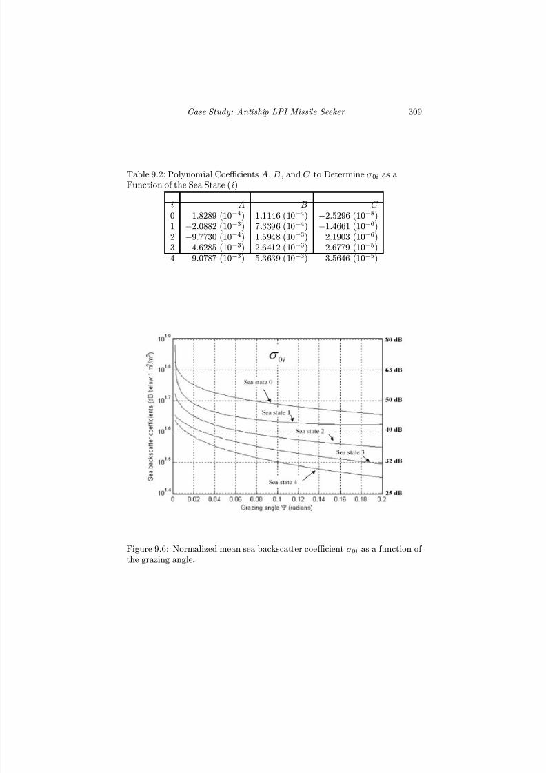
7/17/2019 1596932341 Intercept Radar.pdf
http://slidepdf.com/reader/full/1596932341-intercept-radarpdf 340/891
Case Study: Antiship LPI Missile Seeker 309
Table 9.2: Polynomial Coefficients A, B , and C to Determine σ0i as aFunction of the Sea State (i)
i A B C 0 1.8289 (10−4) 1.1146 (10−4) −2.5296 (10−8)1 −2.0882 (10−3) 7.3396 (10−4) −1.4661 (10−6)2 −9.7730 (10−4) 1.5948 (10−3) 2.1903 (10−6)3 4.6285 (10−3) 2.6412 (10−3) 2.6779 (10−5)4 9.0787 (10−3) 5.3639 (10−3) 3.5646 (10−5)
Figure 9.6: Normalized mean sea backscatter coefficient σ0i as a function of the grazing angle.

7/17/2019 1596932341 Intercept Radar.pdf
http://slidepdf.com/reader/full/1596932341-intercept-radarpdf 341/891
310 Detecting and Classifying LPI Radar
teresting to note that the sea state of one backscatter coefficient does notincrease as dramatically as the other sea states when the grazing angle getslarger. Also note that these clutter calculations minimize the fact that theclutter distribution becomes highly non-Gaussian at low grazing angles, dueto sea spikes. For increased accuracy, lognormal, Weibull, or K-distributedanalysis can be used and will typically increase the required SNR by 10—20dB. In the next section, the transmitter power management is discussed. Thebackscatter coefficient polynominals are then used to predict the detectioncapability of the LPI emitter design for three RCS values (50, 100, 500 m2).
9.4.3 Linear FMCW Emitter Power Management
In a power-managed seeker, the emitter transmits a power level consistent
with the RCS and range of the target to be detected, thereby keeping theSNR a constant. When the missile first enters the engagement envelope andturns on the seeker, the most probable range cells are monitored, and thetransmitter output power is at a level where detection of the target can bemade on a single scan using only a few modulation periods. If the target isnot detected, the power can be increased gradually on the next scan. Oncethe target is detected, the seeker shuts down and the missile moves up to anew location, making any subsequent targeting or exploitation of the emitterimpossible. The emitter uses computer control so that the RF energy is onlyemitted when it is necessary to measure the target characteristics and updatethe track file.
From (1.28), the average transmit power of an FMCW emitter can bewritten as
P CW = (4π)3kT 0F RL∆f
G2tλ
2
R4T
SNRRo
σT
= K
R4T
SNRRo
σT
(9.2)
where L2 ≈ 1, F R is the receiver noise factor, kT 0 = 4.0 × 10⁻²¹ W/Hz,L = LRT LRR represent the system losses, SNRRo is the required outputsignal-to-noise ratio required for target detection, ∆f = 1/tm is the filterbandwidth, RT is the range to the target (ship), and σT is the ship’s RCS.
Continuing with the FMCW example discussed in Chapter 4,f c = 9.3 GHz and tm = 1 ms. The modulation bandwidth is chosen as∆F = 15 MHz in order to provide a ∆R = 10m such that the ship returnall lies within a range bin. Also, F R = 10 and L = 10, which is reasonablefor a single antenna implementation. The antenna is a circular aperture with
diameter da = 0.3m with uniform illumination. This antenna diameter willeasily fit in the nose of an ASCM pod. The 3-dB beamwidth in the azimuthplane depends on the aperture size and is approximately [11]
θa = 1.29 λ
darad (9.3)
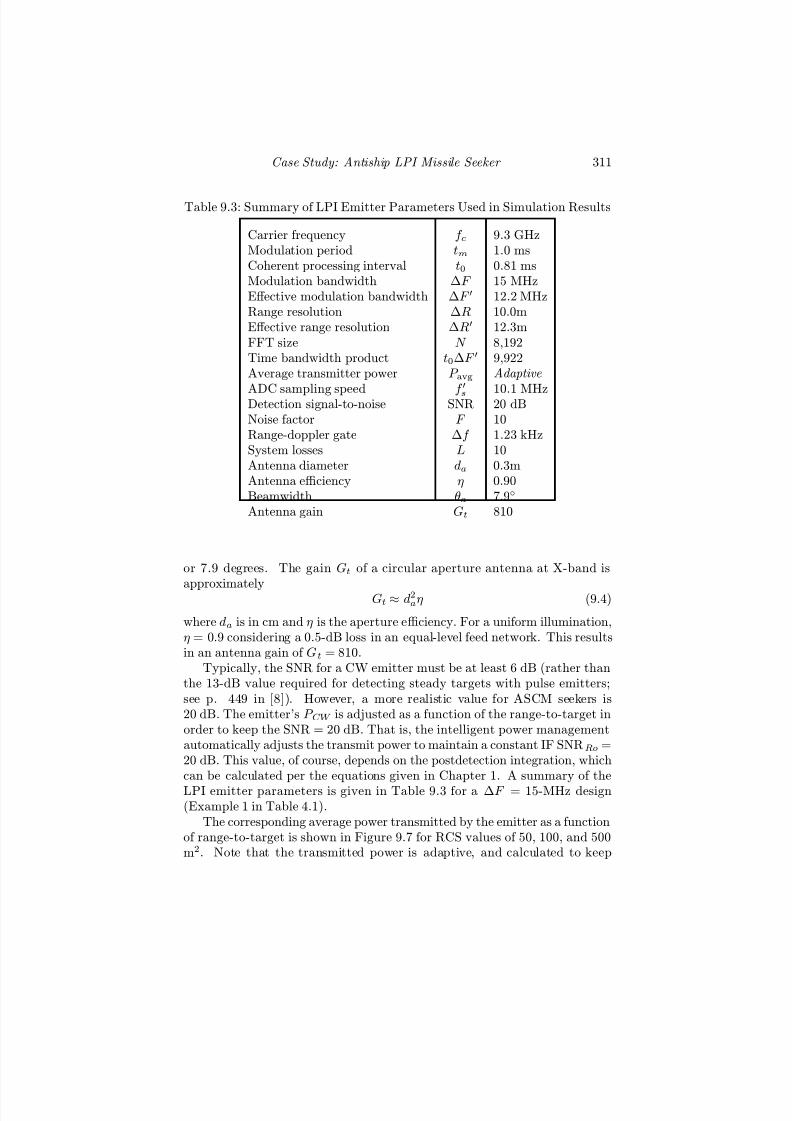
7/17/2019 1596932341 Intercept Radar.pdf
http://slidepdf.com/reader/full/1596932341-intercept-radarpdf 342/891
Case Study: Antiship LPI Missile Seeker 311
Table 9.3: Summary of LPI Emitter Parameters Used in Simulation Results
Carrier frequency f c 9.3 GHzModulation period tm 1.0 msCoherent processing interval t0 0.81 msModulation bandwidth ∆F 15 MHzEff ective modulation bandwidth ∆F 12.2 MHzRange resolution ∆R 10.0mEff ective range resolution ∆R 12.3mFFT size N 8,192Time bandwidth product t0∆F 9,922Average transmitter power P avg Adaptive
ADC sampling speed f
s 10.1 MHzDetection signal-to-noise SNR 20 dBNoise factor F 10Range-doppler gate ∆f 1.23 kHzSystem losses L 10Antenna diameter da 0.3mAntenna efficiency η 0.90Beamwidth θa 7.9
Antenna gain Gt 810
or 7.9 degrees. The gain Gt of a circular aperture antenna at X-band is
approximately Gt ≈ d2aη (9.4)
where da is in cm and η is the aperture efficiency. For a uniform illumination,η = 0.9 considering a 0.5-dB loss in an equal-level feed network. This resultsin an antenna gain of Gt = 810.
Typically, the SNR for a CW emitter must be at least 6 dB (rather thanthe 13-dB value required for detecting steady targets with pulse emitters;see p. 449 in [8]). However, a more realistic value for ASCM seekers is20 dB. The emitter’s P CW is adjusted as a function of the range-to-target inorder to keep the SNR = 20 dB. That is, the intelligent power managementautomatically adjusts the transmit power to maintain a constant IF SNRRo =20 dB. This value, of course, depends on the postdetection integration, whichcan be calculated per the equations given in Chapter 1. A summary of theLPI emitter parameters is given in Table 9.3 for a ∆F = 15-MHz design(Example 1 in Table 4.1).
The corresponding average power transmitted by the emitter as a functionof range-to-target is shown in Figure 9.7 for RCS values of 50, 100, and 500m2. Note that the transmitted power is adaptive, and calculated to keep

7/17/2019 1596932341 Intercept Radar.pdf
http://slidepdf.com/reader/full/1596932341-intercept-radarpdf 343/891
312 Detecting and Classifying LPI Radar
Figure 9.7: Average power transmitted by LPI emitter as a function of rangeto the target and target RCS value.
the total echo power from the target a constant. Also note that only for the50 and 100 m2 case does the transmit power exceed 100W. From (1.34) thetargets echo power from the CW emitter (with L2 = 1 and LRT = LRR = 1)is
P RT = P CW G
2tλ2σT
(4π)3R4T
L W (9.5)
and is a constant (P RT = −140 dBW). In summary, the seeker uses theFMCW waveform and adaptive power management to achieve the LPI char-acteristics. With higher RCS targets, the transmitted power can be reducedeven further.
9.4.4 Target-to-Clutter Ratio
Since the primary purpose of the FMCW emitter is to detect and track shiptargets in the presence of sea clutter, the target-to-sea clutter ratio within
a range bin is examined for sea states 0 to 4 and ship RCS values 50, 100,and 500 m2. Using the backscatter coefficients σ0i, the power of the clutterwithin the target’s range bin can be estimated as
P RC = P CW G
2tλ2σ0iRT θa∆R
(4π)3R4T
L W (9.6)
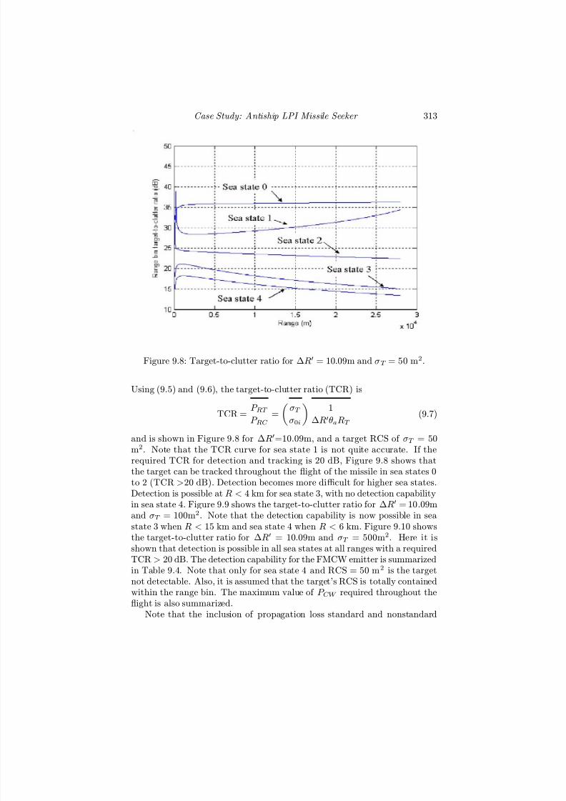
7/17/2019 1596932341 Intercept Radar.pdf
http://slidepdf.com/reader/full/1596932341-intercept-radarpdf 344/891
Case Study: Antiship LPI Missile Seeker 313
Figure 9.8: Target-to-clutter ratio for ∆R = 10.09m and σT = 50 m2.
Using (9.5) and (9.6), the target-to-clutter ratio (TCR) is
TCR = P RT
P RC = σT
σ0i 1
∆R
θaRT
(9.7)
and is shown in Figure 9.8 for ∆R=10.09m, and a target RCS of σT = 50m2. Note that the TCR curve for sea state 1 is not quite accurate. If therequired TCR for detection and tracking is 20 dB, Figure 9.8 shows thatthe target can be tracked throughout the flight of the missile in sea states 0to 2 (TCR >20 dB). Detection becomes more difficult for higher sea states.Detection is possible at R < 4 km for sea state 3, with no detection capabilityin sea state 4. Figure 9.9 shows the target-to-clutter ratio for ∆R = 10.09mand σT = 100m2. Note that the detection capability is now possible in seastate 3 when R < 15 km and sea state 4 when R < 6 km. Figure 9.10 showsthe target-to-clutter ratio for ∆R = 10.09m and σT = 500m2. Here it isshown that detection is possible in all sea states at all ranges with a required
TCR > 20 dB. The detection capability for the FMCW emitter is summarizedin Table 9.4. Note that only for sea state 4 and RCS = 50 m2 is the targetnot detectable. Also, it is assumed that the target’s RCS is totally containedwithin the range bin. The maximum value of P CW required throughout theflight is also summarized.
Note that the inclusion of propagation loss standard and nonstandard

7/17/2019 1596932341 Intercept Radar.pdf
http://slidepdf.com/reader/full/1596932341-intercept-radarpdf 345/891
314 Detecting and Classifying LPI Radar
Figure 9.9: Target-to-clutter ratio for ∆R = 10.09m and σT = 100 m2.
Figure 9.10: Target-to-clutter ratio for ∆R = 10.09m and σT = 500 m2.

7/17/2019 1596932341 Intercept Radar.pdf
http://slidepdf.com/reader/full/1596932341-intercept-radarpdf 346/891
7/17/2019 1596932341 Intercept Radar.pdf
http://slidepdf.com/reader/full/1596932341-intercept-radarpdf 347/891
316 Detecting and Classifying LPI Radar
[4] Jurcheck, J., “Visualizing the littoral battlespace,” Surface Warfare, Vol. 22,pp. 10—15 Aug. 1997.
[5] Zinger, W. H., and Krill, J. A., “Mountain top: Beyond-the-horizon cruisemissile defense,” Johns Hopkins APL Technical Digest, Vol. 18, No. 4, pp.501—520, 1997.
[6] Hitney, H. V., “Refractive Eff ects from VHF to EHF Part A: PropagationMechanisms,” Propagation Modeling and Decision Aids for Communications,
Radar and Navigation Systems, NATO AGARD Lecture Series 196, Ottawa,Canada, Oct. 1994.
[7] Hitney, H. V., “Refractive Eff ects from VHF to EHF Part B: Propaga-tion Models,” Propagation Modeling and Decision Aids for Communications,Radar and Navigation Systems, NATO AGARD Lecture Series 196, Ottawa,Canada, Oct. 1994.
[8] Nathanson, F. E., Radar Design Principles, Second Edition, McGraw-HillInc., New York, 1991.
[9] Paulus, R. A., “Evaporation duct eff ects on sea clutter,” IEEE Trans. on
Antennas and Propagation, Vol. 38, No. 11, pp. 1765—1771, Nov. 1990.
[10] Chan, H. C., Radar sea-clutter at low grazing angles,” IEE Proc. Part F ,Vol. 137, No. 2, pp. 102—112, April 1990.
[11] Barton, D. K., Modern Radar Systems Analysis, Artech House, Inc., Nor-wood, MA, pp. 155, 1988.
[12] “Defense information and infrastructure common operating environment—User’s manual for advanced refractive eff ects prediction system,” SPAWARSystems Command, METOC Systems Program Office, Jan. 9, 2003.
Problems
1. It is an easy matter to modify the second-order polynomial describingthe normalized mean sea backscatter σ0i as a function of grazing an-gle for the five sea states (useful when better empirical data might beobtained). Recall that these coefficients were derived by curve fittingthe values given by Nathanson [8]. The polynomial coefficients (p0—p4)are used in ascm.m and can be regenerated by adjusting the backscat-ter coefficients in clutter polynomial x.m (y0bs through y4bs). (a) Runlpi fmcw design.m to design the ∆F = 15 MHz LPI seeker discussedin Section 7.4. (b) Edit the file clutter polynomial x.m and change thesea state three normalized mean sea backscatter values to
y3bs = [53 46 40 39 37] (9.8)

7/17/2019 1596932341 Intercept Radar.pdf
http://slidepdf.com/reader/full/1596932341-intercept-radarpdf 348/891
Case Study: Antiship LPI Missile Seeker 317
(horizontal polarization). (c) Run the scenario discussed above usingascm.m and compare the detection performance against the vertical po-larization results given in the text (plot the results from both designson the same graph). (d) Summarize the detection range for this hori-zontally polarized seeker.
2. Using the programs lpi fmcw design.m, clutter polynomial x.m and ascm.m,(a) summarize the detection capability of the 9.3-GHz seeker discussedin Section 9.4 if the modulation bandwidth is changed to ∆F = 25MHz. (b) summarize the detection capability if the seeker in (a) keepsthe SNR = 13 dB (instead of 20 dB).

7/17/2019 1596932341 Intercept Radar.pdf
http://slidepdf.com/reader/full/1596932341-intercept-radarpdf 349/891
7/17/2019 1596932341 Intercept Radar.pdf
http://slidepdf.com/reader/full/1596932341-intercept-radarpdf 350/891
Chapter 10
Network-Centric Warfare
and Netted LPI Radar
Systems
LPI radar systems can be networked together into a system of systems tocovertly gather and share surveillance and targeting data as part of a network-centric warfare architecture. In this chapter, network-centric warfare conceptsare introduced including the information grid (network), the sensor grid, andthe weapons grid. A set of metrics is presented to quantify the value addedto an operation by the network. Electronic attack on the network is also con-sidered. Advantages of netted LPI radar systems (part of the sensor grid) arediscussed, including the improvement in emitter sensitivity that is gained, anda multiple-input multiple-output (MIMO) signal model is presented. Network
analysis and netted radar system analysis are presented. Simulation resultsusing LPIsimNet are shown. LPIsimNet is a MATLAB program includedwith the CD that allows the user to evaluate any general netted radar con-figuration and the operational performance of a sensor network. OrthogonalPSK, FSK, and noise waveforms for netted LPI radar applications are alsopresented. Use of MIMO techniques for OTHR is discussed.
10.1 Network-Centric Warfare
In a platform-centric naval architecture the aircraft carrier is the “epicenter”of power. Each weapon has its own sensor and if that sensor is remote there isa stovepipe communication system transmitting the data back to the shooter.
Ultimately, this makes necessary many platforms to eff ectively project the
319
7/17/2019 1596932341 Intercept Radar.pdf
http://slidepdf.com/reader/full/1596932341-intercept-radarpdf 351/891
320 Detecting and Classifying LPI Radar
power needed on the battlespace. Platform-centric command and control(C2) also suff ers limitations in its ability to coordinate operations. For ex-ample, in suppression of enemy air defense (SEAD) operations, the standoff
jammer suff ers significant geometrical problems in alignment, making it diffi-cult to detect and jam coherent threats. The geometrical limitations result inan extended standoff range being necessary and consequently an ineff ective jammer management.
Over the past several years there has been a major shift away fromplatform-centric warfare concepts. Currently we no longer have access tomasses of ships and large numbers of weapons. Also, the weapons today areprecise and must be employed at exactly the right time and place. No singlesensor has the precision to target these advanced technology eff ectors. Theyrequire a dynamic knowledge of the target set and the integration of manysensors and databases.
Evolving from platform-centric warfare, network-centric warfare (NCW)
integrates a distributed system of C2, sensors and weapons called a grid .NCW can extend the capabilities of sensors and weapons across all the plat-forms on the network to pursue the maximum efficiency in mission execution.The grid provides the capability to collect, process and disseminate an unin-terrupted flow of C2, sensors and weapons information between nodes whileexploiting and denying the adversary’s ability to do the same (informationsuperiority)[1]. In contrast to platform-centric warfare, which has an additive
eff ect on combat power (N nodes, total force value = N ), NCW has an expo-
nential eff ect (N nodes, total force value = N 2). The exponential advantagein total force value also gives a maneuver and time-critical strike advantageto the NCW nodes. A more formal definition of NCW is given below.
Definition 10.1
Network-centric warfare is military operations that exploit state-of-the-art sensor information and networking technologies to in-tegrate widely dispersed human decision makers, weapons, situ-ational and targeting sensors and forces into a highly adaptivecomprehensive system to achieve unprecedented mission eff ective-ness.
The NCW grid is composed of three subgrids; the global information grid,the sensor grid and the shooter grid as shown in Figure 10.1 [1]. The global
information grid is a deployed tactical sensor and weapons network that pro-vides the infrastructure for plug-and-play of sensors and shooters. It existsin space, low- and high-Earth orbit, and at all altitudes on land and un-dersea. It is a physical, permanent and fault-tolerant network that receives,
processes, transports, stores and protects the information. It makes availablecommunications and sensor data to the war fighter and is self-organizing,self-monitoring and continuously available. Also provided are adaptive and

7/17/2019 1596932341 Intercept Radar.pdf
http://slidepdf.com/reader/full/1596932341-intercept-radarpdf 352/891
Network-Centric Warfare and Netted LPI Radar Systems 321
Figure 10.1: Network-centric architecture employing an information grid,shooter grid, and a sensor grid. The sensor grid is composed of a nettedLPI radar system of systems.
automated decision aids. The number of nodes directly reflects a volume of
force on the network and the information processing capability required. Thenetwork topology represents the configuration of the links to integrate thesensor and weapons nodes.
The sensor grid is composed of air-, sea-, ground-, space-, and cyberspace-based sensor nodes. Netted LPI radar systems play an important part toprovide “at all levels” a covert surveillance capability and high degree of situ-ational awareness. In this type of netted radar systems, a number of transmit-ters and receivers are spatially distributed with each receiver being capable of processing signals scattered by the target from every transmitter. In addition,weapons can also be targeted using the netted LPI emitters. An increase in aradar’s target processing capability (local node processing) benefits the speedof relaying the targeting information. The sensor grid is a transient grid andexists only for the task at hand. It is reformed for every mission with the
collaborative C2 performing dynamic sensor tasking and data fusion. Withthe benefits of new network assurance technology, topologies are now capableof providing a more robust network for information fusion. Sensor network
7/17/2019 1596932341 Intercept Radar.pdf
http://slidepdf.com/reader/full/1596932341-intercept-radarpdf 353/891
322 Detecting and Classifying LPI Radar
protocols are described in [2] and secure routing techniques in the presenceof electronic attack are described in [3].
The shooter grid consists of both weapons and jammers. It enables the joint war fighter to plan and execute operations in a manner that achievespower projection at a precise time and place. By exploiting the battlespaceawareness, new operational capabilities are realized including the executionof time-critical missions, and the rapid acquisition and execution of targetsin a timely manner. The shooter grid is also a transient grid where the pieceparts are physical. The grid exists for the task only and is reformed for everymission. In Figure 10.1, the NCW architecture is used to track a low RCStarget using a netted LPI sensor grid (advantages of netting the distributedradar systems together are discussed in Section 10.5). The target is disabledwith a missile from the weapons grid.
10.1.1 NCW Requirements
There are several requirements for NCW operations. To achieve a force thatis network-centric, a wideband RF transmit/receive capability is required tocompress and transport large amounts of data. Also required is a wideband lo-cal area network which can process and transmit information locally betweenthe sensors and/or weapons. Eff ective information management or the abil-ity to efficiently use, process and apply information is also required. Finally,a critical mass of platforms, sensors, and weapons that have the informa-tion processing capability is required. When forming the NCW architecture,questions to be answered include: How do diff erent degrees of networking im-pact the strategic, operational and tactical outcomes? What is the optimalnetwork topology (physical, virtual, arrangement of nodes)? How will thenetwork impact the C2? What is the correct balance of sensors, shooters and
network technology? Can we quantify how the network processing sustainsdegradation from events such as an electronic attack?The answer to these questions is difficult since there are complex rela-
tionships between the network space and the battlespace. For example, fromthe information standpoint, the overall information processing capability ismainly determined by the number of nodes, the individual node capability,and the topology of the network as shown in Figure 10.2. Note that thisfigure does not show information flow but shows an overall relationship de-pendence. For example, the number and distribution of LPI emitters on anetwork must be sufficient to build a precise and timely picture of the bat-tlespace taking into account the limited detection ranges available. The datadistribution and data association between nodes must correlate the data accu-rately avoiding any misidentification. The increase in information processing
capability sequentially results in an enhancement in the situational aware-ness and operational tempo that aff ect the maneuverability, decision speed,lethality, and agility on the battlefield.

7/17/2019 1596932341 Intercept Radar.pdf
http://slidepdf.com/reader/full/1596932341-intercept-radarpdf 354/891
Network-Centric Warfare and Netted LPI Radar Systems 323
Figure 10.2: Relationship between network space and battlespace
10.1.2 Situational Awareness
Situational awareness is defined by the U.S. Army’s Training and DoctrineCommand as “the ability to have accurate real-time information of friendly,enemy, neutral, and noncombatant locations; a common, relevant picture of the battlefield scaled to specific levels of interest and special needs” [4]. TheLPI radar sensor can provide a critical role in maintaining the required situa-tional awareness since it is able to gather the information without injecting aninfluence. That is, the radar sensor used to gather the information should berequired to have a low probability of intercept. If detection by enemy nonco-operative intercept receivers occurs, an enemy response will ensue increasing
the characteristic tempo λT uncontrollably. The characteristic tempo is de-fined as the speed in which the situational awareness is processed in order toorient (or adjust) the force to the current situation. In practice, situationalawareness is built by continuous snapshots that are gathered from the bat-tlefield and transferred to the commander. A larger information gatheringability (e.g., more nodes) results in a larger information volume enabling forexample, beyond line-of-sight targeting. Better information exchange abilityresults in a quick refreshing of the snapshot. Consequently, the situationalawareness is mainly determined by the information processing capability [5].
10.1.3 Maneuverability
A far-reaching netted radar system of systems can also improve force maneu-verability, which is the capability to perform a strategic or tactical movement.To evaluate the maneuverability performance, we consider three of its prop-

7/17/2019 1596932341 Intercept Radar.pdf
http://slidepdf.com/reader/full/1596932341-intercept-radarpdf 355/891
324 Detecting and Classifying LPI Radar
Figure 10.3: Improvement in maneuverability.
erties: speed, safety, and cost. Maneuverability can be promoted throughthe support of situational awareness. Figure 10.3 shows the improvement inmaneuverability when a network-enabled situational awareness is eff ective [6].For example, better terrain awareness results in optimal route design. Theroute design not only increases the speed of the maneuver, but it can alsoreduce the probability of risk and possibly result in a lower cost. Anotherexample is better threat awareness which helps the preparation of a properoff ense and contributes to improvements in maneuverability. Furthermore,better integration of coalition war fighters into battlespace actions can alsoincrease force maneuverability.
10.1.4 Decision Speed and Operational Tempo
The observation-orientation-decision-action (OODA) loop is important foroperations and has become a critical concept in military strategy. John Boydoriginally developed the concept to explain how to direct one’s energies todefeat an enemy and survive [7]. The OODA loop concept is shown in Fig-ure 10.4. A war-fighting enterprise that can process the entire OODA cyclequickly, observing and reacting to unfolding events more rapidly than an op-ponent, can “get inside” the opponent’s decision cycle and gain a militaryadvantage. The LPI radar nodes and the characteristic tempo λT play a sig-nificant part in the observation-to-orientation phase of the OODA loop. Thedecision tempo λC 2 is defined as the speed to make a decision to act. Afterthe decision to act is made, the speed at which action is taken is the sum of the characteristic tempo and a deployment tempo λd. After deployment, thespeed at which the situational response (or fighting) is made is the sum of the characteristic tempo and a fi ghting tempo λf . These individual temposcan be used to quantify the maximum operational tempo of the network-an
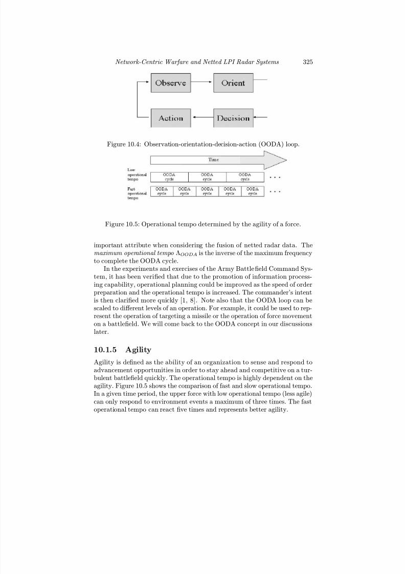
7/17/2019 1596932341 Intercept Radar.pdf
http://slidepdf.com/reader/full/1596932341-intercept-radarpdf 356/891
Network-Centric Warfare and Netted LPI Radar Systems 325
Figure 10.4: Observation-orientation-decision-action (OODA) loop.
Figure 10.5: Operational tempo determined by the agility of a force.
important attribute when considering the fusion of netted radar data. Themaximum operational tempo ΛOODA is the inverse of the maximum frequencyto complete the OODA cycle.
In the experiments and exercises of the Army Battlefield Command Sys-tem, it has been verified that due to the promotion of information process-ing capability, operational planning could be improved as the speed of orderpreparation and the operational tempo is increased. The commander’s intent
is then clarified more quickly [1, 8]. Note also that the OODA loop can bescaled to diff erent levels of an operation. For example, it could be used to rep-resent the operation of targeting a missile or the operation of force movementon a battlefield. We will come back to the OODA concept in our discussionslater.
10.1.5 Agility
Agility is defined as the ability of an organization to sense and respond toadvancement opportunities in order to stay ahead and competitive on a tur-bulent battlefield quickly. The operational tempo is highly dependent on theagility. Figure 10.5 shows the comparison of fast and slow operational tempo.In a given time period, the upper force with low operational tempo (less agile)
can only respond to environment events a maximum of three times. The fastoperational tempo can react five times and represents better agility.

7/17/2019 1596932341 Intercept Radar.pdf
http://slidepdf.com/reader/full/1596932341-intercept-radarpdf 357/891
326 Detecting and Classifying LPI Radar
10.1.6 Lethality
Lethality is the ability to damage an enemy. Only with the sufficient situa-
tional awareness and efficient operational tempo can the forces perform withthe best lethality. The radar sensor network plays a key role in the measure of lethality. For example, the artillery can perform with high lethality with ac-curate targeting information and timely approval of attack. Infantry attacksalso do well with enough intelligence and under quick and timely command.It is important to note that if the enemy is aware of the targeting informa-tion being gathered, the characteristic tempo is slowed due to the furtherreconnaissance that is necessary. The lethality of the action is also severelydegraded emphasizing the need for the battlefield sensors to be LPI.
10.2 Metrics for Information Grid Analysis
A military sensor and weapons grid is sometimes assumed to have an infinitenumber of nodes each with a similar capability. In the analysis, this oftenleads to misleading results, especially when a small number of dissimilar nodesare used [8]. This section examines the network theory and metrics that aredesigned to quantify the general value inherent in the information networktopology. These include the connectivity measure, the network reach, andthe network richness. Combining these metrics with the operational tempospreviously discussed, we can quantify the maximum operational tempo of thenetwork. The presence of an electronic attack is also addressed.
10.2.1 Generalized Connectivity Measure
A time-dependent, generalized connectivity measure (C M ) of a network of
sensors and weapons is defined as the sum of the value of all the nodes andtheir connections scaled by the lengths of the routes and their directionality.The connectivity measure can be expressed as [8]
C M (t) =N T μ=1
K μ(t)
N μν =1
N μ,νγ =1
Lμ,ν γ (d, t) (10.1)
where N T is the number of nodes in the network, N μ is the total number of nodes connected to the node μ, N μ,ν is the total number of possible routesconnecting the pair of nodes μ and ν , K μ(t) is the capability value of nodeμ, and relates to the ability of the node to process and transfer informationquickly. Lμ,ν
γ is the information fl ow parameter of the route γ connectingnodes μ and ν and depends on the length of the route d and is also a function
of time t. The capability and information flow parameters have the range0 ≤ K μ(t), Lμ,ν
γ ≤ 1. For the examples below, we use a normalized value forthe route length d. That is, d = 1 from one node to another.

7/17/2019 1596932341 Intercept Radar.pdf
http://slidepdf.com/reader/full/1596932341-intercept-radarpdf 358/891
Network-Centric Warfare and Netted LPI Radar Systems 327
Figure 10.6: Three node example to demonstrate generalized connectivity
link calculations.
Table 10.1: List of All Available Links in Figure 10.6
Links
1 → 32 → 12 → 33 → 13 → 2
The term “route” is the possible connection from one node to anothernode. The term “link” represents the direct connection between any twonodes. One route contains at least one or more links. Figure 10.6 showsthree information nodes deployed with diff erent capability values K μ. Thelink from node μ = 1 to node μ = 2 is not available. A list of all availablelinks and routes are shown in Tables 10.1 and 10.2, respectively.
The functional dependence of Lμ,ν γ on the length of the route d (number
of links) and time t can be simplified by separating it into a time-independentcomponent Lμ,ν and a time dependent flow coefficient F μ,ν γ (t), which is scaledby the route length d raised to the power ξ . The expression for C M (t) thenbecomes [8]
C M (t) =N T
μ=1
K ν (t)
N μ
ν =1
Lμ,ν
N μ,ν
γ =1
F μ,ν γ (t)
(dγ )ξ (10.2)
The value of F μ,ν γ (t) is a minimum of zero and reaches a maximum of onewhen the route γ is capable of supporting all information exchanges. Note the

7/17/2019 1596932341 Intercept Radar.pdf
http://slidepdf.com/reader/full/1596932341-intercept-radarpdf 359/891
328 Detecting and Classifying LPI Radar
Table 10.2: List of All Possible Routes
Start Node End Node Routes1 2 1 → 3 → 21 3 1 → 32 1 2 → 1
2 → 3 → 12 3 2 → 3
2 → 1 → 33 1 3 → 1
3 → 2 → 13 2 3 → 2
Figure 10.7: Two nodes with a unidirectional link.
order of the node superscripts matters. For example, consider the two nodesshown in Figure 10.7. The flow coefficient 0 ≤ F μ,ν γ ≤ 1 however, F ν ,μγ = 0.
To illustrate these ideas, assume K μ(t) is time independent and that anytwo nodes are either connected or not (F μ,ν γ (t) = 0 or 1). The directionalityof the information is also included. Also assume that the scaling exponentξ = 1, and the time independent information flow parameter Lμ,ν = 1 forevery route are identical. As a result, (10.2) can be simplified to
C M (t) =N T μ=1
K μN μν =1
N μ,νγ =1
F μ,ν γ (t)
dγ (10.3)
In summary, the following assumptions are held. First, the connectivity istime-independent. That is, K μ(t) = K μ and F μ,ν γ (t) = F μ,ν γ . Also, ξ = 1 andany two nodes are either connected (or not). Table 10.3 demonstrates thegeneralized connectivity C M calculation for Figure 10.6.
10.2.2 Reference Connectivity Measure
The reference connectivity measure (C RM ) is defined to represent a fully con-nected network configuration. The reference network has all nodes fully con-
nected with bidirectional links [8]. In addition, each node has a capabilityvalue of K μ = 1. For example, Figure 10.8 shows a realistic four-node infor-mation transfer network deployed with diff erent capability values K μ. There

7/17/2019 1596932341 Intercept Radar.pdf
http://slidepdf.com/reader/full/1596932341-intercept-radarpdf 360/891
Network-Centric Warfare and Netted LPI Radar Systems 329
Table 10.3: Calculation of Connectivity Measure
C M Route K μ dγ Contribution
1 → 3 → 2 1 2 0.5001 → 3 1 1 1.0002 → 1 0.75 1 0.7502 → 3 → 1 0.75 2 0.3752 → 3 0.75 1 0.7502 → 1 → 3 0.75 2 0.3753 → 1 0.25 1 0.2503 → 2 → 1 0.25 2 0.1253 → 2 0.25 1 0.250
C M = 4.375
is a unidirectional link from node 1 to node 2 and from node 3 to node 2.There are also two bidirectional links from node 3 to node 1 and from node 3to node 4. Figure 10.9 shows the corresponding reference network for Figure10.8. Note that all the nodes are homogeneous and connected to one another(fully connected) and that all capability values are K μ = 1 and F μ,ν γ = 1 forall γ ,μ and ν . The reference connectivity measure only depends on the totalnumber of nodes N T and is calculated as
C RM = N T (N T −1)×
1 +
N T − 2
2 + · · · +
(N T − 2)(N T − 3) · · · 2 · 1
N T − 1
(10.4)
The term outside the square brackets in (10.4), N T (N T − 1), represents the
number of possible connections in a given network with N T nodes. Thenumerator in each term inside the square brackets is the number of possibleroutes of the length given in the denominator. The reference network hasthe highest connectivity measure of any network with same number of nodes.Table 10.4 shows the value of C RM for 3 ≤ N T ≤ 8 and shows the exponentialincrease in C RM with a linear increase in the number of nodes.
10.2.3 Network Reach
The reference connectivity measure C RM provides a means to normalize theconnectivity measure (10.3) resulting in the network reach I R as [8]
I R = C M
C R
M
(10.5)
which is a dimensionless quantity. Normalization by the reference networkallows us to investigate varying degrees of network connection, nonidentical

7/17/2019 1596932341 Intercept Radar.pdf
http://slidepdf.com/reader/full/1596932341-intercept-radarpdf 361/891
330 Detecting and Classifying LPI Radar
Figure 10.8: Realistic four-node sensor network configuration.
Figure 10.9: Reference network for the radar information network shown inFigure 10.8.
Table 10.4: List of Reference Connectivity Measures
Node Number C RM 3 94 325 1206 534
7 2,9058 18,976

7/17/2019 1596932341 Intercept Radar.pdf
http://slidepdf.com/reader/full/1596932341-intercept-radarpdf 362/891
Network-Centric Warfare and Netted LPI Radar Systems 331
nodes/links and the eff ect of broken symmetries due for example, to electronicattack of the network.
10.2.4 Suppression Example
A network-enabled SEAD example with N T = 5 is considered in Figure 10.10.In this scenario, we are concerned with the capability of the network to trans-fer sensor data efficiently. To suppress the Eagle (Ka-band battlefield sur-veillance and missile control radar), an EA-6B is networked with an RQ-1Predator, an AC-130 Gunship and an EA-18G. The EA-6B, the gunship andthe EA-18G are all data linked to the special operations forces on the ground(note the unidirectional flow of information).
The capability value K μ is assigned as shown for each asset. The capabilityvalue depends on the platform’s level of networking and ability to participatein the data and information exchange needed. For the example, both theEA-6B and the EA-18G have a value K = 1.0 since they are in control of the suppression mission and are fully network capable. The RQ-1 Predatoris assigned a value of K = 0.5 since it cannot relay directly to the specialoperation forces, any of its images and data that are gathered. The AC-130 gunship is assigned K = 0.85 since it is somewhat less capable than theEA-18G and EA-6B due to its multimission characteristics. Note that thespecial operation forces are assigned K = 0.3 and is a low value since theyonly receive images and data and do not transmit (otherwise they would givetheir position away).
The reference connectivity measure is calculated first. For N T = 5,
C RM = 5(4) ×
1 +
3
2 +
3 · 2
3 +
3 · 2 · 1
4
(10.6)
or C RM = 120. Note that this value only depends on the number of nodesparticipating in the network. Using this value, the expression for the networkreach is
I R = 1
120
N T =5μ=1
K μ
N μν =1
Lμ,ν
⎛⎝N μ,ν
γ =1
F μ,ν γ
dγ
⎞⎠ (10.7)
The values for N μ = N 1 = 4, N 2 = 3, N 3 = 4, N 4 = 4, N 5 = 3. Also,N 11 = 0. The value of N 12 = 5 can be verified from Figure 10.10. That is,there are five routes from node 1 to node two. The five routes are shown inTable 10.5. With L12 = 1, the summation of the flow coefficients scaled bythe route lengths is
F
1,2
d = 11 + 12 + 12 + 13 + 13 = 2.67 (10.8)
Continuing on, the other node to node flow coefficients scaled by the route

7/17/2019 1596932341 Intercept Radar.pdf
http://slidepdf.com/reader/full/1596932341-intercept-radarpdf 363/891
332 Detecting and Classifying LPI Radar
Figure 10.10: Eagle radar suppression using N T = 5 nodes.
lengths can be calculated. The network reach is then
I R = 1120
(1.0[3(2.67) + 4.33] + 0.5[3(2.67) + 5] +
0.85 [3(2.67) + 4.33] + 1.0[3(2.67) + 4.33] + 0) = 0.3473(10.9)
The fi
rst four terms in brackets are the EA-6B, RQ-1A, AC-130 and theEA-18G respectively. The zero term (last term) is due to the fact that thisnode contributes nothing to the overall information transfer capability of thenetwork. The low value of network reach is due to the reduction in nodecapability values and the loss of sensor information rerouting options. Notethat if the capability value K = 1.0 for all nodes in the above example, then
Table 10.5: Five Routes Identified from Node 1 to Node 2
1 2 3 4 5
1 1 1 1 12 3 4 4 3
2 2 3 42 2

7/17/2019 1596932341 Intercept Radar.pdf
http://slidepdf.com/reader/full/1596932341-intercept-radarpdf 364/891
Network-Centric Warfare and Netted LPI Radar Systems 333
I R = 0.4167.
10.2.5 Extended Generalized Connectivity MeasureWe can generalize (10.3) by considering the case where 0 < F μ,ν γ < 1 exists(partial efficiency of route). For instance, if a traversed node on one routehas a low capability (K μ 1), this route will not be able to maintain fullcapability in the flow of sensor information [6]. Consider for example thenetwork shown in Figure 10.6. The route node 1 → node 3 → node 2 isevaluated as K 1/dγ = 1/2 = 0.5. However, the traversed node K 3 = 0.25gives indication that the sensor information flow from node 1 to node 3 cannotbe efficiently exchanged via node 3. Taking the limitation of the traversedintermediate nodes into account, from (10.3) we get an extended definition of connectivity measure as
C Me(t) =
N T μ=1
N μν =1
N μ,νγ =1
K γ F
μ,ν
γ dγ
(10.10)
where K γ represents the K μ with the lowest capability value (bottleneck) inroute γ . Note the fact that K γ in the route only considers the starting nodeand exchangers; the receiving node is not included. This consideration is dueto the fact that many nodes in military networks only accept the informationwithout an equivalent information processing capability in transmitting. Forinstance, in route node 1 → node 3 → node 2, only the transmitter (node1) and exchanger (node 3) are available for assignment to K γ to reflect thebottleneck of the information flow. For the same route, shown in Figure10.6, the extended C M is recalculated as shown in Table 10.6. Comparing toTable 10.3, notice the value of C M decreases from 4.375 to 3.75 due to the
consideration of the bottlenecks in route 1 → 3 → 2 and 2 → 3 → 1 reflectinga more realistic capability.
In summary, the robustness of the network can be quantified by comparingC M to C RM , and by disabling nodes in the reference and the real networkand recalculating C M and C RM . By comparing these values, a representationappears of the real network behavior while under attack. In fact, the rate of change (degradation) in the value of the connectivity measure as a functionof the number of links severed and nodes being attacked can provide goodinsight into the robustness of the sensor network.
10.2.6 Entropy and Network Richness
At each node or source, the rate at which information is sent has a direct
impact on the operational tempo of the grid. Consider the set of J possiblesample values (or source symbols) by S = x1, . . . , xJ . We assume the
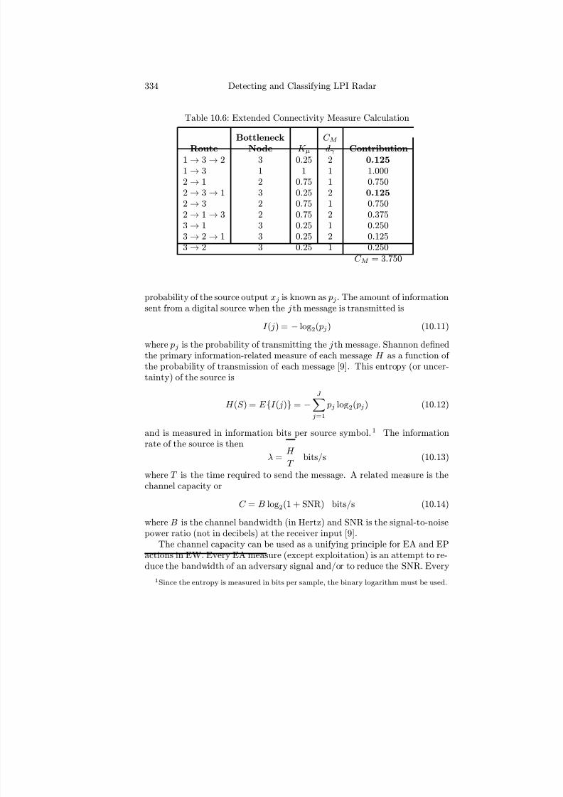
7/17/2019 1596932341 Intercept Radar.pdf
http://slidepdf.com/reader/full/1596932341-intercept-radarpdf 365/891
334 Detecting and Classifying LPI Radar
Table 10.6: Extended Connectivity Measure Calculation
Bottleneck C M Route Node K μ dγ Contribution
1 → 3 → 2 3 0.25 2 0.125
1 → 3 1 1 1 1.0002 → 1 2 0.75 1 0.7502 → 3 → 1 3 0.25 2 0.125
2 → 3 2 0.75 1 0.7502 → 1 → 3 2 0.75 2 0.3753 → 1 3 0.25 1 0.2503 → 2 → 1 3 0.25 2 0.1253 → 2 3 0.25 1 0.250
C M = 3.750
probability of the source output xj is known as pj . The amount of informationsent from a digital source when the j th message is transmitted is
I ( j) = − log2( pj) (10.11)
where pj is the probability of transmitting the j th message. Shannon definedthe primary information-related measure of each message H as a function of the probability of transmission of each message [9]. This entropy (or uncer-tainty) of the source is
H (S ) = E I ( j) = −
J
j=1
pj log2( pj) (10.12)
and is measured in information bits per source symbol.1 The informationrate of the source is then
λ = H
T bits/s (10.13)
where T is the time required to send the message. A related measure is thechannel capacity or
C = B log2(1 + SNR) bits/s (10.14)
where B is the channel bandwidth (in Hertz) and SNR is the signal-to-noisepower ratio (not in decibels) at the receiver input [9].
The channel capacity can be used as a unifying principle for EA and EP
actions in EW. Every EA measure (except exploitation) is an attempt to re-duce the bandwidth of an adversary signal and/or to reduce the SNR. Every
1Since the entropy is measured in bits per sample, the binary logarithm must be used.
7/17/2019 1596932341 Intercept Radar.pdf
http://slidepdf.com/reader/full/1596932341-intercept-radarpdf 366/891
Network-Centric Warfare and Netted LPI Radar Systems 335
EP action (except protection against exploitation) is an attempt to increasebandwidth and/or increase SNR.
Example 1: The LPI emitter uses frequency hopping as an EP measure anduses a large total bandwidth to protect against jamming, but a small instanta-neous bandwidth to protect against interception and exploitation. The largetotal bandwidth in this case makes it difficult for the jammer to set on thetransmission frequency, thus limiting the reduction in SNR to that providedby barrage jamming.
Example 2: Repeater or gate stealing EA techniques must achieve a certainreduction of SNR within the bandwidth of the victim’s receiver to be eff ec-tive. The corresponding EP technique might utilize a combination of guardsand filters to recognize and eliminate the unwanted jamming signal, therebyprotecting the SNR.
Example 3: Against exploitation, a LPI emitter uses a very large bandwidthwith low average power density. The low average power reduces the probabil-ity of intercept, but the energy over the bandwidth can be summed to extractthe information from the signal. Therefore, the transmitter compensates forthe low SNR with increased bandwidth to transmit the information at a fastenough rate. The jammer can only achieve high SNRs over small portions of the bandwidth.
Each node within the sensor network is able to process the information ata certain rate. The information processing rates of each node can be combinedto quantify the network’s richness. The information rate, λμ, of a node μ, isthe rate at which the network information is processed by the node (in Hz).
The minimum information rate, λminμ , of the node is the minimum rate that
information must be processed for generating decision-level knowledge fromthe sensor network data. From Shannon’s information entropy theory, theknowledge function is defined as [8]
Q (λμ) =
⎧⎪⎪⎨⎪⎪⎩
0, if λμ < λminμ
ln λμλminμ
, if λmin
μ < λμ < e · λminμ
lne·λmin
μ
λminμ
= 1, if λμ ≥ e · λmin
μ
(10.15)
Using the knowledge function, the network richness RQ is defined to representthe average rate at which information entropy (or knowledge) is generatedfrom the sensor data shared through the network or [8]
RQ =
N T μ=1 λμQ(λμ)
N T s−1 (10.16)

7/17/2019 1596932341 Intercept Radar.pdf
http://slidepdf.com/reader/full/1596932341-intercept-radarpdf 367/891
336 Detecting and Classifying LPI Radar
Figure 10.11: Time spent in each phase in OODA cycle. ( After [8].)
From this equation, if a node cannot provide the knowledge at a rate above itsminimum value, the node’s contribution λμQ(λμ) degrades the overall valueRQ. In addition, there is little advantage to generating sensor data fasterthan knowledge can be generated and absorbed.
10.2.7 Maximum Operation Tempo
A network has a maximum information exchange rate that is determined bythe number of nodes, the communication and sensor technologies employed,the information data transfer rates, and the network topology. To quantifythis rate within an OODA, a characteristic tempo (λT ) is defined and relatesthe network topology and its ability to gather the situational awareness. Thecharacteristic tempo for the network is the product of the network reach I Rand the network richness RQ
λT = I RRQ Hz (10.17)
and relates the information exchange capability of the sensor network. Inaddition, for every command and control structure (and associated doctrine),there is a characteristic decision-making rate (λC 2) or speed at which decisionsare made using the transferred sensor data being processed [10].
Figure 10.11 shows the tempo parameters of the sensor network OODAloop. The variable ∆t1 represents the time from observation to orientationand is limited by the information exchange time, ∆t2 is the time from ori-entation to decision and is dominated by the decision speed, ∆t3 is the timefrom decision to action and must be greater than the information exchange
time (command time) and deployment time, and ∆t4 is the time from actionto observation and is always greater than the sum of information exchangetime and fighting time.

7/17/2019 1596932341 Intercept Radar.pdf
http://slidepdf.com/reader/full/1596932341-intercept-radarpdf 368/891
Network-Centric Warfare and Netted LPI Radar Systems 337
Using the OODA tempo parameters, the maximum operation tempo of thenetwork (ΛOODA) is of interest and represents the maximum tempo of thenetwork to perform an entire OODA including responding to events as
ΛOODA ≤
1
λT +
1
λC 2+
1
λT +
1
λd+
1
λT +
1
λf
−1
(10.18)
or after some algebra
ΛOODA ≤ λC 2
1 + 1λd
+ 1λf
λC 2 + 3λC2
λT
(10.19)
Note that λC 2 in the numerator emphasizes that the fact that while technol-ogy can help increase the network and action tempos, the C2 tempo plays alimiting role not helped by technology alone [8]. Also note that in practice theoperational tempo is not a fixed value. The operational tempo calculated hererepresents the maximum value due to the limitation of the network topologyand nodes capabilities. It provides a direct link between the internal metricsof the network and the operational outcome of a sensor and weapons networkthrough a single equation. It is also significant in that it enables direct evalua-tion of the networks capability to collect, process and disseminate information(information superiority) to the combat outcome (battlespace superiority).
10.3 Electronic Attack
Jamming of the information grid is a form of electronic attack and can takeon many forms such as partial band jamming, and tone jamming [11]. Theeff ectiveness of the jamming waveform depends on the signaling format used
to transfer the data and the type of jamming used. When a jammer is takeninto consideration, the jam-to-signal ratio (JSR) at the victim node’s receivercauses a link failure to occur if the jam-to-signal ratio is greater than a par-ticular threshold causing the bit error rate to be unacceptable. Figure 10.12shows a jammer (node 4) added into the previous example shown in Figure10.6.
The JSR is determined by many factors including jamming and signalpower, jammer range, jamming strategy, RF waveform bandwidth, and prop-erties of the receiver. To simplify the calculation, considering only power andrange, the JSR in a single information link can be written as
JSR = ERPJ /4π(RJ )
2
ERPC /4π(RC )2 =
ERPJ ERPC
RC RJ
2
(10.20)
where ERPJ is the eff ective radiated power of the jammer (node 4), ERPC isthe eff ective radiated power of the data/communication signal emitted from

7/17/2019 1596932341 Intercept Radar.pdf
http://slidepdf.com/reader/full/1596932341-intercept-radarpdf 369/891
338 Detecting and Classifying LPI Radar
Figure 10.12: Addition of a jammer into the node configuration shown inFigure 10.6.
node 3 to node 1, RC is the range from node 3 to node 1, and RJ is the rangefrom the jammer at node 4 to the receiver at node 1.
The capability values can be assigned and used within the JSR calculationto quantify the jammer eff ectiveness. The capability values are defined asfollows. The value of K μ is defined as the information-processing capabilityof the receiving node μ and its importance to the network. Assuming theimportance of the information transferred through each node is not diff erent,we see that the K μ is related to the information exchange capability. Also,K J ν is the jamming capability of the hostile jammer and is defined as theinformation link jamming capability at node ν . Similar to K μ, 1 ≥ K J ν ≥ 0and is determined by factors such as its eff ective radiated power, jammerwaveform type, and jamming strategy. Without a loss in generality, theratio of K J ν to K μ is set equal to the ratio of the eff ective radiated powers.
Therefore, (10.20) can be written as
JSR = ERPJ ERPC
RC RJ
2
= K J ν K μ
RC RJ
2
(10.21)
The JSR is used to represent the eff ect of the jamming on an existing infor-mation exchange link. When the JSR is higher than a given threshold, theinformation link is regarded as unavailable.
10.4 Information Network Analysis Using
LPIsimNet
The MATLAB folder LPIsimNet (see Appendix D) provides the tools to cal-culate the metrics discussed above and generates a visual summary of thesimulation results for any user-defined global information grid configuration.

7/17/2019 1596932341 Intercept Radar.pdf
http://slidepdf.com/reader/full/1596932341-intercept-radarpdf 370/891
Network-Centric Warfare and Netted LPI Radar Systems 339
In this section, several simulations are presented to illustrate the metrics dis-cussed above including the eff ects of an electronic attack. The label notationused is in the form of (i, j) XYZ. The i represents the node type and can beany one of the following:
• N: Friendly information/data transfer communication node;
• R: Friendly LPI radar node (discussed in the next section);
• NR: Friendly node with both information/data transfer capability andradar capability;
• JN: Hostile communication jammer node;
• JR: Hostile radar jammer node;
• JNR: Hostile communication and radar jammer node.
The j indicates the index of the node and ranges from 1 to the number of nodes utilized N T . The XYZ represents the name of the node (e.g., EA-6B,E2C).
The first simulation considers a sensor network with three nodes as shownin Figure 10.13. In this simulation, the communication between an E-2C, anF-16 and an AC-130 are being studied. Figure 10.14 shows the scenario setupused to generate the simulation. Note that the user can control the numberand characteristics of each node within the scenario (including the placementand movement). Top-level properties are in rows 2 through 5. Rows 6 through10 show the characteristics of the individual nodes. The last section showsthe node connectivity. For the simulation shown in Figure 10.13, there aretwo bidirectional links and one unidirectional link indicated by the direction
arrows. The simulation is run and the results are summarized in Table 10.7.The sensor network simulation results can be generated for any number of nodes and connectivity but can take a significantly longer period of time forsimulations with a large number of nodes. The details of the connectivitymeasure C M and network richness RQ are shown in Tables 10.8 and 10.9,respectively.
To quantify the eff ect of an electronic attack, a jammer onboard a RussianSu-34 is added to the sensor network. The sensor network under attack isshown in Figure 10.15. The Russian Su-34 is located at the bottom rightcorner and is represented by a hollow circle. The jamming connection is shownby a dashed line to E-2C. The initial scenario configuration is shown in Table10.16. The total time index row represents the number of time indexes thatare calculated in the simulation. This off ers the ability to include movement
of all assets. For the setup shown in Figure 10.15, total time indexes is setto 3. When the simulation is run, the jammer moves closer to the E-2C ateach time index and all metrics are recalculated (total of 3 times). Position

7/17/2019 1596932341 Intercept Radar.pdf
http://slidepdf.com/reader/full/1596932341-intercept-radarpdf 371/891
340 Detecting and Classifying LPI Radar
Figure 10.13: Three communication nodes.
Table 10.7: Simulation Results of Scenario Shown in Figure 10.13
Results Values
Reference connectivity measure 9Connectivity measure 3.75Network reach 0.42Network richness 271.60Characteristic tempo 113.16Operational tempo 26.78

7/17/2019 1596932341 Intercept Radar.pdf
http://slidepdf.com/reader/full/1596932341-intercept-radarpdf 372/891
Network-Centric Warfare and Netted LPI Radar Systems 341
Table 10.8: Analysis Detail of Connectivity Measure for Simulation Shown inFigure 10.13
Bottleneck C M Route Node Contribution
1 → 3 → 2 3 0.1251 → 3 1 1.0002 → 1 2 0.7502 → 3 → 1 3 0.1252 → 3 2 0.7502 → 1 → 3 2 0.375
3 → 1 3 0.2503 → 2 → 1 3 0.1253 → 2 3 0.250
C M = 3.750
Table 10.9: Analysis Detail of Network Richness for Simulation Shown inFigure 10.9
Node λ Q (λ/λm) λQ (λ/λm)1 200 0.69315 138.6302 200 0.69315 138.6303 300 1.7918 537.540
814.800RQ = 814.8/3 = 271.600

7/17/2019 1596932341 Intercept Radar.pdf
http://slidepdf.com/reader/full/1596932341-intercept-radarpdf 373/891
342 Detecting and Classifying LPI Radar
Figure 10.14: User setup of the scenario shown in Figure 10.13.
refers to the initial position of the node and velocity indicates the movementof each node per time index (km/time index).
A summary of the simulation results for the three time instances is shown
in Figure 10.15 (time index 1), Figure 10.17 (time index 2), and Figure 10.18(time index 3).
Note that for each time instant, the jammer is moving closer to the E-2C.Notice on the second time index, the jammer is close enough to disable one of the links. The node 3 to 1 link is disabled due to the JSR > 1. On the thirdindex, the link from node 2 to 1 is also suppressed. Consequently, severaltrends in the network metrics can be noted across the three time indexes. Asthe jammer moves towards the network, the measure of connectivity decreasesas does the network reach. Also, a noticeable decrease in the characteristictempo and maximum operational tempo is shown.
10.5 Netted LPI Radar Systems
Despite recent advances in monostatic radar systems (colocated single trans-mitter and receiver), two major disadvantages are inherent. They off er little
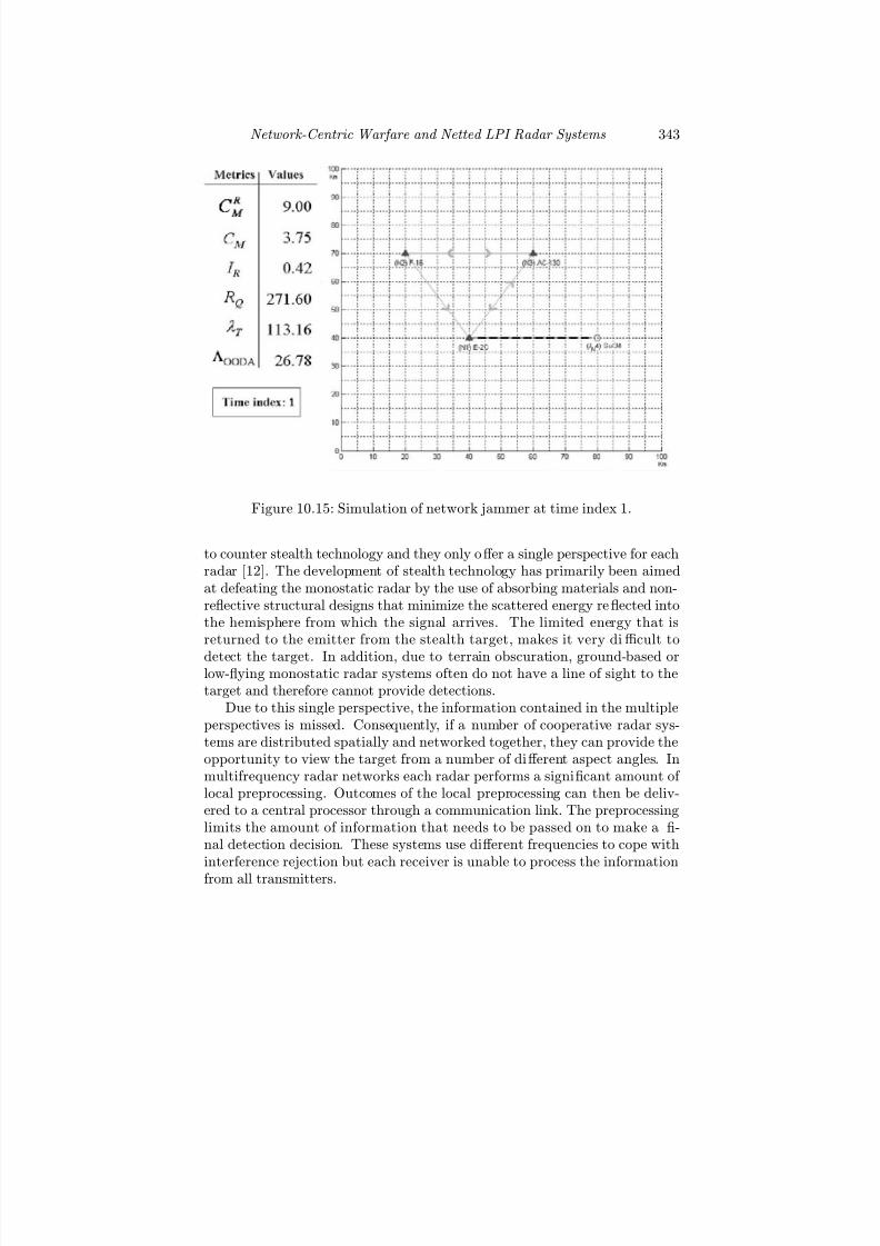
7/17/2019 1596932341 Intercept Radar.pdf
http://slidepdf.com/reader/full/1596932341-intercept-radarpdf 374/891
Network-Centric Warfare and Netted LPI Radar Systems 343
Figure 10.15: Simulation of network jammer at time index 1.
to counter stealth technology and they only off er a single perspective for eachradar [12]. The development of stealth technology has primarily been aimedat defeating the monostatic radar by the use of absorbing materials and non-reflective structural designs that minimize the scattered energy reflected intothe hemisphere from which the signal arrives. The limited energy that isreturned to the emitter from the stealth target, makes it very difficult to
detect the target. In addition, due to terrain obscuration, ground-based orlow-flying monostatic radar systems often do not have a line of sight to thetarget and therefore cannot provide detections.
Due to this single perspective, the information contained in the multipleperspectives is missed. Consequently, if a number of cooperative radar sys-tems are distributed spatially and networked together, they can provide theopportunity to view the target from a number of diff erent aspect angles. Inmultifrequency radar networks each radar performs a significant amount of local preprocessing. Outcomes of the local preprocessing can then be deliv-ered to a central processor through a communication link. The preprocessinglimits the amount of information that needs to be passed on to make a fi-nal detection decision. These systems use diff erent frequencies to cope withinterference rejection but each receiver is unable to process the information
from all transmitters.

7/17/2019 1596932341 Intercept Radar.pdf
http://slidepdf.com/reader/full/1596932341-intercept-radarpdf 375/891
344 Detecting and Classifying LPI Radar
Figure 10.16: User setup of the scenario shown in Figure 10.15.
Netted radar systems sometimes referred to as spatial multiple-inputmultiple-output (MIMO) radar systems, consist of a number of distributedradar systems (transmit and receive sensors) each having the ability to trans-
mit independent orthogonal waveforms (to avoid interference) and the abilityto receive and process synchronously all waveforms that are transmitted. Fig-ure 10.19 shows an example of a netted radar system with three radar nodesconnected by a network. All three radars have already acquired and are track-ing the target with their antenna beams. The radar systems R1, R2, and R3each transmit a diff erent waveform but receive and process all three waveformsthat are collected from the target. The use of the network allows each systemto share its target information noncoherently (using orthogonal waveforms)or coherently where each radar has a common precise knowledge of space andtime. The implementation of networked radar systems has become feasibledue to recent advances in large bandwidth wireless networks, high-capacitytransmission lines, multichannel electronically scanned antennas, high-speedlow-cost digital processors and precise synchronization systems [13].

7/17/2019 1596932341 Intercept Radar.pdf
http://slidepdf.com/reader/full/1596932341-intercept-radarpdf 376/891
Network-Centric Warfare and Netted LPI Radar Systems 345
Figure 10.17: Simulation of network jammer at time index 2.
Figure 10.18: Simulation of network jammer at time index 3.

7/17/2019 1596932341 Intercept Radar.pdf
http://slidepdf.com/reader/full/1596932341-intercept-radarpdf 377/891
346 Detecting and Classifying LPI Radar
Figure 10.19: Example of a sensor network connecting three LPI emitters(R1, R2, R3).
10.5.1 Advantages of the Netted LPI Radar Systems
There are two important characteristics of a netted radar system; the spa-tial dispersion of the nodes (i.e., transmitter and receiver locations) and thedata fusion processing (i.e., processing performed in the receiver at a nodeto combine multiple receiver outputs). These characteristics lead to severaladvantages of a netted LPI radar system.
The spatial distribution (or geometry) of the nodes enable the surveil-lance area to be tailored according to the specific mission objective [14]. Themultisite emitters can be used to form a specially designed surveillance areato more efficiently detect targets based on known patterns of military be-havior. The network also allows a multiperspective SAR or ISAR image tobe generated. By using a number of distributed transmitters and receiversto collect the echos from the target at diff erent aspects or directions, theindependent angular samples provide spatial diversity of the target’s RCS.With widely separated antennas, netted radar systems also have the abilityto handle slow moving targets by exploiting Doppler estimates from multipledirections. If coherent processing is used, high-resolution target localizationcan be achieved with a resolution that far exceeds that supported by theradar’s waveform [15]. This however, comes with a price. The receivingand processing requirement for such a coherent summation is highly demand-ing. For example, if each waveform produces 1,000 resolvable range cells and
10 Doppler cells, integration would be required simultaneously in 10, 000N
2
cells (possibly reduced by excluding regions not mutually covered). Given thehigh-resolution in both range and Doppler, the numbers used here may in-

7/17/2019 1596932341 Intercept Radar.pdf
http://slidepdf.com/reader/full/1596932341-intercept-radarpdf 378/891
Network-Centric Warfare and Netted LPI Radar Systems 347
crease by orders of magnitude, straining the capability of most modern signalprocessors.
One of the inherent properties of the netted radar system is the increasein the number of degrees of freedom due to the spatial diversity [14, 16].The scattered reflections can be captured to take advantage of the targetscintillation providing a gain in detection performance. The spatial diversitycan be used to separate scattering centers from one another that otherwisecause a glint signature. In addition, targets can be more easily separated fromthe clutter in clutter-limited detection scenarios [17]. The target’s RCS spatialvariations can also be exploited to obtain a diversity gain for estimation of various parameters (e.g., angle of arrival, Doppler). Target classification andrecognition can be improved as a result of the extra information retrievedfrom the diff erent perspectives [18]. With more degrees of freedom, flexibletime-energy management modes can be utilized to minimize the amount of energy that is radiated. Since more of the scattered energy from the target is
collected (from diff
erent directions), the sum of the ERP from all the radarsystems can be made approximately equivalent to that of a single monostaticradar [19]. As a result, the detection performance of the system is superiorwhile also utilizing a minimum ERP. A better system sensitivity results dueto the additional transmitters and receivers which augment the total receivedsignal power leading to an increase in overall SNR. Further, every node is lessvulnerable to physical and electronic attack—increased survivability. That is,the destruction of the sensor network by an ARM is less likely. The probabilityof being coherently jammed is also less likely since the probability of interceptis lowered even further.
The likelihood of obtaining a line-of-sight to the target is also greatlyimproved due to the spatial dispersion of the radar nodes [20]. 2 Having severalradar systems will add confusion to the noncooperative intercept receiver
that has to cope with the increased number of signals. Another significantadvantage is the increase in the reliability of the netted radar system. Theloss of one or even several nodes may not destroy the surveillance capabilitybut more of a graceful degradation will take place as there are still othernodes available [14].
There are also technical challenges to be addressed. The most importantis the time and frequency synchronization for coherent operation. By usingGPS as a reference timing signal, the network can be made coherent. Anotherimportant challenge is the data fusion and registration of the various datastreams, which requires reliable and high-capacity communication links inthe network [14].
2One of the disadvantages of bistatic and multistatic radar systems is that more thanone line-of-sight path is required. For low-altitude targets, the network of monostatic radars
has a much higher probability of having at least one unusable path. The more nodes thatrequire simultaneous line-of-sight paths, the lower the probability of success.

7/17/2019 1596932341 Intercept Radar.pdf
http://slidepdf.com/reader/full/1596932341-intercept-radarpdf 379/891
348 Detecting and Classifying LPI Radar
10.5.2 Netted LPI Radar Sensitivity
The spatially distributed and networked LPI radar system of systems can
be broken down into a set of M × N transmitter-receiver pairs each with abistatic component contributing to the entirety of the netted radar sensitivity[13]. Figure 10.19 can be considered as a connected series of bistatic radarsystems where the transmitter and receiver are separated. With this, it isnecessary to calculate the target-to-transmitter range and target-to-receiverrange separately. These range values then replace the single range term inthe monostatic radar equation. In addition, a separate bistatic RCS value foreach bistatic radar pair must be computed. Thermal noise at each receivercan be assumed to be statistically independent. The overall netted radar SNRcan be calculated by summing up the partial SNR of each transmitter-receiverpair as [12, 19]
SNRnet =
M i=1
N j=1
P CW iGtiGrjσTijλ2i
(4π)3kT 0ijBRiR2tiR
2rjF RjLij (10.22)
where P CW i is the ith average CW transmitter power, Gti is the ith transmitantenna gain, Grj is the jth receive antenna gain, σTij is the RCS of the targetfor the ith transmitter and j th receiver, λi is the ith transmitted wavelength,BRi is the bandwidth of the matched filter for the ith transmitted waveform,k is Boltzmann’s constant, T 0ij is the receiving system noise temperature at aparticular receiver, F Rj is the noise factor for each receiver, Lij is the systemloss for the ith transmitter, jth receiver (Lij > 1), Rti is the distance fromthe ith transmitter to the target and Rrj is the distance from the target tothe jth receiver. Note that this assumes that all signals can be separatelydistinguished at each receiver and that all antenna beams are pointed at the
target. Also note that with i = j = 1, (10.22) reverts to the monostatic case.An important characteristic of netted radar systems can be identified whenwe consider each radar to be identical with every transmitter-receiver com-bination the same [12]. In this case the netted radar SNR equation can bewritten as
SNRnet = P CW GtGrσT λ2
(4π3)kT 0BF RL
M i=1
N j=1
1
R2tiR
2rj
(10.23)
Insight is gained if we group all of the range independent parameters togetherinto a constant K , then the netted radar SNR can be expressed as
SNRnet =M i=1
N j=1
K
R2tiR
2rj
(10.24)

7/17/2019 1596932341 Intercept Radar.pdf
http://slidepdf.com/reader/full/1596932341-intercept-radarpdf 380/891
Network-Centric Warfare and Netted LPI Radar Systems 349
Normalizing (10.24) by the SNR for a single monostatic radar (10.37) we have
SNRnetSNR1
= R4
M i=1
N j=1
1
R2tiR
2rj
(10.25)
which shows that the SNR of the system is related to the power receivedfrom the contributing transmit and receive paths. Further, if Rti = Rrj andM = N it follows that [19]
SNRnetSNR1
∝ N 2 (10.26)
That is, the system SNR is a function of the square of the number of nodes forcoherent operation. This represents an N -fold improvement over the nonco-herent case (γ = 0.5). For noncoherent netted radar processing, the numberof transmit antennas serves as a factor in the number of diversity paths. Forcoherent processing the number of transmit antennas contributes to reduc-ing the spurious peaks. In either mode, the processing at the receiver scansthrough all the possible target locations.
It must be pointed out that for each of the N radars to receive and processthe N diff erent waveforms transmitted by those radars all with antenna gainsGt and Gr, achieving SNRnet applies to the sum of N 2 coherently combinedsignals. Since antenna gain G ≈ 4π/Ψb where Ψb is the solid angle within thehalf-power beam contour, there are in the hemisphere visible to each radar2π/Ψ = G/2 beam positions. Unless the target has been acquired and placedin track by a single radar, using the single-radar (monostatic) SNR availableto that radar, and used to point the other radars, the probability that allradars illuminate the target simultaneously is extremely small for GtGr 1.
This implies that near omni-directional antennas must be used to achieveinitial detection based on SNRnet. If designation from a monostatic radaris used, then the other radars must each place a transmitting and receivingbeam on each target for which SNRnet is to be obtained, implying either nearomnidirectional or multiple directional beams that require splitting transmit-ter energy amongst multiple targets. In summary, for most cases SNRnet willonly be available for tracking or identifying a target that is first detected bya single monostatic radar in the network.
10.5.3 Signal Model
To develop the netted radar (spatial MIMO) signal model, a distributed tar-get with Q independent isotropic scatterers is considered. Figure 10.20 shows
four such scatterers located in a 2-D plane along with the M LPI trans-mitters T k = (xtk, ytk), k = 1, . . . , M that illuminate the target and the N receivers Rl = (xrl, yrl), l = 1, . . . , N that collect the scattered energy. We let

7/17/2019 1596932341 Intercept Radar.pdf
http://slidepdf.com/reader/full/1596932341-intercept-radarpdf 381/891
350 Detecting and Classifying LPI Radar
E/Msk(t) be the set of transmitted waveforms where E is the total trans-
mitted energy. Normalization by M makes the total energy independent of thenumber of transmitters used to illuminate the target [18]. The target reflec-tivity can be expressed in a diagonal Q×Q matrix with
= diag(ξ 1, . . . , ξ Q).
The target average RCS is E [tr(T
)] = 1 and is independent of the num-ber of scatterers. For the netted radar case, spatial diversity is achieved withthe distributed antenna positions. The M waveform generators (W Gk) trans-mit orthogonal (noncoherent) waveforms in order that the energy from thediff erent transmitters may be easily separated at the receiver where each of the receive antennas has M matched filters (MF 1i . . . M F M i with one corre-sponding to each orthogonal waveform).
Neglecting the path loss and summing over all of the scatterers, the totalsignal received can be expressed as
zlk(t) =
E
M
Q
q=1
ξ qsk[t− τ tk(X q)− τ rl(X q)]e−j2πf c[τ tkX(q)+τ rl(Xq)] (10.27)
where τ tk(X q) = d(T k, X q)/c is the propagation time delay between thekth transmitting sensor and the scatterer at X q. The distance d(T k, X q) =
(xtk − xq)2 + (ytk − yq)2. The propagation time delay τ rlX (q ) is definedanalogously. The two exponential terms in (10.27) reflect the phase shift dueto the propagation from transmitter k to scatterer q and the phase shift dueto the propagation from the scatterer q to the receiver l.
The channel components of (10.27) are often collected as [18]
h(q)lk = ξ qe−j2πf c[τ tk(Xq)+τ rl(Xq)] (10.28)
and can be interpreted as the equivalent “channel” between transmitter k,scatter q and receiver l. The channel element (10.28) consists of e−j2πf cτ tk(Xq)
which is the phase shift due to the propagation from transmitter k to scattererq . Similarly, e−j2πf cτ rl(Xq) is the phase shift due to the propagation from thescatterer q to the receiver l. The reflectivity of the scatterer is ξ q. With(10.28), (10.27) can be expressed as
zlk(t) =
E
M
Qq=1
h(q)lk sk[t− τ tk(X q)− τ rl(X q)] (10.29)
If the target has an RCS center of gravity at X 0 = (x0, y0) and we assumethat sk(t− τ tk(X q)− τ rl(X q)) ≈ sk(t− τ tk(X 0)− τ rl(X 0)) for all q = 1, . . . , Qthen
zlk(t) =
E
M hlksk[t− τ tk(X q)− τ rl(X q)] (10.30)
wherehlk =
Qq=1
h(q)lk (10.31)

7/17/2019 1596932341 Intercept Radar.pdf
http://slidepdf.com/reader/full/1596932341-intercept-radarpdf 382/891
Network-Centric Warfare and Netted LPI Radar Systems 351
Figure 10.20: Netted radar with M transmit antennas each with a separateorthogonal waveform generator. Receive array consists of N antennas eachwith a parallel set of M matched filters. Target is shown with distributedscatterers located at X q with reflectivity ξ . Target’s RCS center of gravity islocated at X 0.
7/17/2019 1596932341 Intercept Radar.pdf
http://slidepdf.com/reader/full/1596932341-intercept-radarpdf 383/891
352 Detecting and Classifying LPI Radar
Accounting for additive noise, the observed waveforms at the receive antennal can be expressed as
rl(t) =
E M
hlksk[t− τ tk(X 0)− τ rl(X 0)] + wl(t) (10.32)
where wl(t) is the additive circularly symmetric, zero mean, complex Gaussiannoise that is spatially and temporally white with autocorrelation functionσ2wδ (τ ).
Properties of the elements hlk of the channel matrix and the conditionsfor spatial decorrelation E [hlkh∗li] ≈ 0 are further addressed in [18, 21]. Inessence, the spatial decorrelation means that diff erent receive antennas mea-sure a diff erent value of the RCS. Also discussed is the relationship of themodel to other types of emitters such as phased arrays, adaptive radar STAPand multistatic radar. Properties of the MIMO radar ambiguity functions aregiven in [22—24]. As a final point, we point out that the maximum number
of targets K max, that can be uniquely identified simultaneously by a phased array with N receive antenna elements is
K max = 2N
3 (10.33)
while the maximum number of targets that can be uniquely identified simul-taneously by a MIMO radar is [25]
K max = 2MN
3 (10.34)
That is, the maximum number of targets that can simultaneously be uniquelyidentified by a MIMO radar is up to M times its phased array counterpart.
10.5.4 Netted Radar Electronic Attack
The JSR as defined by the jamming power and signal (radar echo) power isgiven by
JSR = jamming power
signal power (10.35)
Unlike communication antennas that often use dipole antennas for omni-directional communication, radar antennas frequently use highly directionalantennas that can identify the target angle in azimuth and elevation. Theshape of the radar antenna pattern (pencil beam) results in degradation of the jamming signal when the jamming signal is not incident on the main lobe.The jam-to-signal ratio is
JSR =
⎛⎝ ERPJ
4π (RJ )2
ERPR
4π (RT )2
⎞⎠ cos θ =
ERPJ ERPR
RT RJ
2
cos θ (10.36)

7/17/2019 1596932341 Intercept Radar.pdf
http://slidepdf.com/reader/full/1596932341-intercept-radarpdf 384/891
Network-Centric Warfare and Netted LPI Radar Systems 353
Figure 10.21: Example of jamming with incident angle.
where ERPJ = P jGj is the eff ective radiated power of the jammer, ERPR =P CW Gt is the eff ective radiated power of the LPI radar, RJ is the range
from the jammer to the radar, RT is the range from the radar to the target,and θ is the incident angle of jamming. Figure 10.21 provides an example of the jamming signal incident with θ = 60 degrees that results in cos θ = 0.5degradation in the jamming power.
10.6 Netted Radar Analysis Using LPIsimNet
The LPIsimNet MATLAB tools (see Appendix D) are used in this sectionto demonstrate the SNR advantages of a netted-radar configuration. Anyuser-defined netted radar configuration can be analyzed [26]. Results are alsoshown when a jammer is included in an electronic warfare topology. We startby examining the SNR contour tools for a monostatic LPI emitter.
10.6.1 Monostatic LPI Emitter and the SNR Contour
Chart
A contour chart represents an important analysis tool to quickly quantify theadvantages of any netted radar sensor network and jammer configuration. Westart by examining the monostatic LPI emitter to present the SNR contourchart that is generated by the MATLAB tools LPISimNet. In a monostaticLPI radar system, the transmitter and receiver are co-located and can onlyintercept a very small portion of the electromagnetic energy scattered fromthe target. Much of the signal and its information is lost.
To introduce the SNR contour analysis, we revisit the monostatic radarconfiguration. The SNR for a monostatic configuration can be written as
SNR1 = P CW GtGrσT λ
2
(4π)3kT 0F RBRR4T L
(10.37)

7/17/2019 1596932341 Intercept Radar.pdf
http://slidepdf.com/reader/full/1596932341-intercept-radarpdf 385/891
354 Detecting and Classifying LPI Radar
To develop a useful analysis tool for an LPI emitter, a contour chart is con-structed with the RCS σT = 1m2. This normalized contour chart can easilybe scaled for any RCS. In addition, the SNR is only dependent on the radarproperties and target range. By plotting the results in a 2-D geometric map,the SNR of the radar can be read as shown in Figure 10.22.
Figure 10.22: Example of SNR contour chart for a monostatic LPI emitter.
This chart illustrates the SNR contour generated by the MATLAB soft-ware contained on the CD (LPIsimNet.m). For this simulation, the Pilotradar is used with an ERPR = P CW Gt = 1,000W, Ae = 0.0815 m2 and isthe eff ective receiving aperture area (equal to Grλ
2/2π), and noise powerkT 0F RBRi = 7.5 × 10⁻¹³W. For any target position selected, the value of SNR can be read from the figure.
10.6.2 Three Netted LPI Emitters
To demonstrate the advantages of a netted LPI radar configuration, threeradar systems are simulated within a 2,500-km2 region using the MATLAB
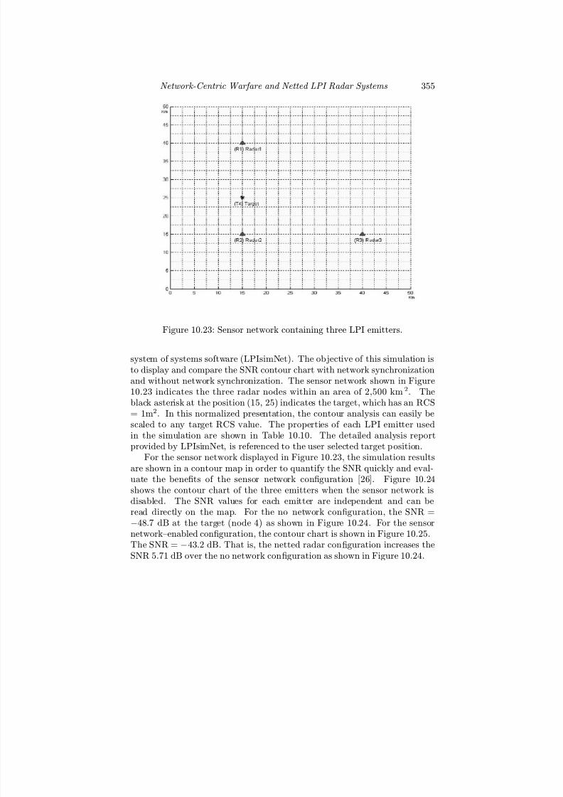
7/17/2019 1596932341 Intercept Radar.pdf
http://slidepdf.com/reader/full/1596932341-intercept-radarpdf 386/891
Network-Centric Warfare and Netted LPI Radar Systems 355
Figure 10.23: Sensor network containing three LPI emitters.
system of systems software (LPIsimNet). The objective of this simulation isto display and compare the SNR contour chart with network synchronizationand without network synchronization. The sensor network shown in Figure10.23 indicates the three radar nodes within an area of 2,500 km 2. Theblack asterisk at the position (15, 25) indicates the target, which has an RCS= 1m2. In this normalized presentation, the contour analysis can easily bescaled to any target RCS value. The properties of each LPI emitter usedin the simulation are shown in Table 10.10. The detailed analysis reportprovided by LPIsimNet, is referenced to the user selected target position.
For the sensor network displayed in Figure 10.23, the simulation resultsare shown in a contour map in order to quantify the SNR quickly and eval-uate the benefits of the sensor network configuration [26]. Figure 10.24shows the contour chart of the three emitters when the sensor network isdisabled. The SNR values for each emitter are independent and can beread directly on the map. For the no network configuration, the SNR =−48.7 dB at the target (node 4) as shown in Figure 10.24. For the sensornetwork—enabled configuration, the contour chart is shown in Figure 10.25.The SNR = −43.2 dB. That is, the netted radar configuration increases the
SNR 5.71 dB over the no network confi
guration as shown in Figure 10.24.

7/17/2019 1596932341 Intercept Radar.pdf
http://slidepdf.com/reader/full/1596932341-intercept-radarpdf 387/891
356 Detecting and Classifying LPI Radar
Table 10.10: LPI Sensor Network: Parameters for the Three Emitter Nodes
Node Index 1 2 3
Type Blue Force Blue Force Blue ForceName Radar1 Radar2 Radar3
ERP (W) 1000 100 10Ae(m2) 0.0815 0.0815 0.0815
Noise Power (W) 7.5 × 10⁻¹³ 1 × 10⁻¹² 1.5 × 10⁻¹²
Position (Km) (15, 40) (15, 15) (30, 25)
Figure 10.24: SNR contour chart for three emitters without sensor network .

7/17/2019 1596932341 Intercept Radar.pdf
http://slidepdf.com/reader/full/1596932341-intercept-radarpdf 388/891
Network-Centric Warfare and Netted LPI Radar Systems 357
Figure 10.25: SNR contour chart for three emitters with sensor network .

7/17/2019 1596932341 Intercept Radar.pdf
http://slidepdf.com/reader/full/1596932341-intercept-radarpdf 389/891
358 Detecting and Classifying LPI Radar
Figure 10.26: Jammer attack on a sensor network containing two LPI emit-ters. Target is 1 m2 at position (15, 25) km.
10.6.3 Two Netted LPI Emitters with Jammer
To quantify the eff ects of an electronic attack on a netted radar system, twoLPI emitters are placed in a topology with the 1-m2 target. A jammer toattack both emitters is added as shown in Figure 10.26. The parameters
for the two LPI emitters and the jammer (onboard an Su-34) are shown inTable 10.11. By comparing the signal-to-jam ratio (SJR) contour chart, withand without networking, the advantages of a sensor network in an electronicwarfare configuration can be identified.
The contour results for the SJR when no network is used are shown inFigure 10.27. The contour results for the SJR when the LPI emitters usea sensor network are shown in Figure 10.28. The SJR improvement in thesensor network case is 5.75 dB.
10.7 Orthogonal Waveforms for Netted Radar
The increased area of coverage using a system of netted radar systems, each
diverse and independent, make netted radar sensing and the developmentof appropriate waveforms an important area of investigation. Multiradarsystems can operate in both monostatic and multistatic modes simultaneously

7/17/2019 1596932341 Intercept Radar.pdf
http://slidepdf.com/reader/full/1596932341-intercept-radarpdf 390/891
Network-Centric Warfare and Netted LPI Radar Systems 359
Table 10.11: LPI Sensor Network: Parameters for the Two Emitters and OneJammer
Node Index 1 2 3
Type Blue Force Blue Force Hostile JammerName Radar1 Radar2 Su-34
ERP (W) 1000 100 10Ae(m2) 0.0815 0.0815 -
Noise Power (W) 7.5 × 10⁻¹³ 1 × 10⁻¹² -Position (Km) (15, 40) (15, 15) (30, 25)
Figure 10.27: SJR for jammer attack on two LPI emitters. Target is 1 m2 at
position (15, 25) km.
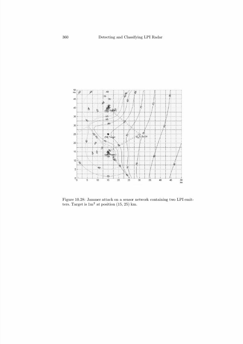
7/17/2019 1596932341 Intercept Radar.pdf
http://slidepdf.com/reader/full/1596932341-intercept-radarpdf 391/891
360 Detecting and Classifying LPI Radar
Figure 10.28: Jammer attack on a sensor network containing two LPI emit-ters. Target is 1m2 at position (15, 25) km.

7/17/2019 1596932341 Intercept Radar.pdf
http://slidepdf.com/reader/full/1596932341-intercept-radarpdf 392/891
Network-Centric Warfare and Netted LPI Radar Systems 361
and can retain the favorable features of both a monostatic radar system anda multistatic radar system if each system transmits a distinct signal from aset of orthogonal signals in which any two signals are not cross-correlated andeach receiver uses multiple matched filters. As discussed in Chapter 5, in orderto achieve high range resolution and multiple target resolution, the periodicautocorrelation function of any transmitted code sequence should have a lowpeak side lobe level (PSL). For moving targets, Doppler loss occurs at thematched filter output of the correlation receiver. For a sequence of length N c,with Doppler shift f d and signal duration T the excessive phase incrementsfrom one sequence to the next is 2πf dT/N c.
Netted LPI radar systems require a code sequence with low PSL, resis-tance to Doppler loss and the use of orthogonal waveforms that have a lowcross-correlation between them. This is to avoid interference and to provideindependent information about the target at various angles. The concept of orthogonal netted radar systems is diff erent than the traditional netted radar
systems. Consider the multiradar system shown in Figure 10.19 consisting of L LPI radar systems where each system transmits a distinct low power CWsignal using an orthogonal code set sl(t), l = 1, 2, 3, . . . , L. Any two signalsin the set are uncorrelated or
C ≈
t
s p(t)s∗q(t + τ )dt = 0 (10.38)
for p = q and p, q = 1, 2, . . . , L. For high-range resolution, the aperiodicautocorrelation function of any code sl(t) in the code set should be close toan impulse function or
A = 1
E
t
sl(t)s∗l (t + τ ) = 1 (10.39)
for τ = 0 and A = 0 otherwise.If the radar stations in the multiradar system transmit signal sl(t), l =
1, 2, 3, . . . , L, respectively, any radar station can choose to receive and processany of the L signals by including a matched filter that correlates to the trans-mitted signal only. The target echoes from the other signals generate near-zero outputs at the matched filter because it does not correlate with any of them. If a radar system is equipped with only a matched filter that correlatesto its own transmitted signal, then the system will only operate in the mono-static mode. If there are multiple parallel matched filters at a receiver thatcorrelate to the signals that are transmitted by other radar stations, multipledetection results of targets are available for integration processing (coherentlyor noncoherently).
The waveforms used by netted radar systems must be carefully designed toavoid the self-interference and detection confusion. An orthogonal waveformset is a group of waveforms in which each of the waveforms has the nearly ideal
7/17/2019 1596932341 Intercept Radar.pdf
http://slidepdf.com/reader/full/1596932341-intercept-radarpdf 393/891
362 Detecting and Classifying LPI Radar
noise-like aperiodic autocorrelation property and any two of them have nocross-correlation. If the emitter transmits the waveforms from an orthogonalcoding waveform set, it can adaptively operate based on the environments andreal-time needs in regular monostatic mode or in a multistatic mode with thesame carrier frequency.
10.7.1 Orthogonal Polyphase Codes
Orthogonal netted radar systems require a set of orthogonal transmit signalswith properties as outlined in (10.38) and (10.39) [27]. Orthogonal polyphasecodes have several advantages for the emitter over the use of binary phasecodes. The orthogonal polyphase codes have a larger main lobe-to-side loberatio than binary signals with the same code length N c. They also have amore complicated signal structure making the signal harder to detect andanalyze by a noncooperative intercept receiver.
The orthogonal polyphase code set consists of L signals with each sig-nal containing N c subcodes and can be represented by the complex numbersequence
sl(n) = ejφl(n) (10.40)
where n = 1, 2, . . . , N c and l = 1, 2, . . . , L where φl(n), (0 ≤ φl(n) < 2π) isthe phase of subcode n of signal l in the signal set. If the number of distinctphases available to be chosen for each subcode in a code sequence is M c,the phase for a subcode can only be selected from the following admissiblevalues [27]
φl(n) ∈
0,
2π
M c, 2 ·
2π
M c, . . . , (M c − 1) ·
2π
M c
(10.41)
orφl(n) = ψ
1,ψ
2, . . . ,ψM
c
(10.42)
Considering a polyphase code set S with code length N c, set size of L anddistinct phase number M c, the phase samples of S can be represented withthe L × N c phase matrix
S (L, N c, M c) =
φ1(1) φ2(2) · · · φ1(N c)φ2(1) φ2(2) · · · φ2(N c)
......
......
φL(1) φL(2) · · · φL(N c)
(10.43)
where the phase sequence in row l is the polyphase sequence of signal l andall the elements in the matrix can only be chosen from the phase set in(10.41), (10.42). From (10.38) and (10.39), it can be shown that the aperiodicautocorrelation of the polyphase sequence sl and cross-correlation properties
7/17/2019 1596932341 Intercept Radar.pdf
http://slidepdf.com/reader/full/1596932341-intercept-radarpdf 394/891
Network-Centric Warfare and Netted LPI Radar Systems 363
of orthogonal polyphase codes s p and sq will satisfy or nearly satisfy [27]
A(φl, k) =⎧⎪⎪⎨⎪⎪⎩
1
N c
N c−kn=1 exp j[φl(n)− φl(n + k)] = 0 0 < k < N c
1N c
N cn=−k+1
exp j[φl(n)− φl(n + k)] = 0 −N c < k < 0
(10.44)for l = 1, 2, . . . , L and
C (φl, k) ≈
⎧⎪⎪⎨⎪⎪⎩
1N c
N c−kn=1
exp j[φq(n)− φ p(n + k)] = 0 0 < k < N c
1N c
N cn=−k+1
exp j[φq(n)− φ p(n + k)] = 0 −N c < k < 0
(10.45)for p = q and p, q = 1, 2, . . . , L where k is the discrete time index.
To design the polyphase code set with the properties given in (10.44) and(10.45), the minimization of a cost function that is based on the total autocor-relation side lobe energy and the cross-correlation energy is performed. Thisminimization then leads to uniformly distributed autocorrelation side lobeand cross-correlation energies among all possible locations thus minimizingthe autocorrelation side lobe peaks and cross-correlation peaks. Given valuesof N c, M c and L, the energy-based cost function used is
E =Ll=1
N c−1k=1
|A(φl, k)|2 + λ
L−1 p=1
Lq= p+1
N c−1k=−(N c−1)
|C (φ p,φq, k)|2 (10.46)
where λ is the weighting coefficient between the autocorrelation function andthe cross-correlation function in the cost function. Minimization of this func-
tion with N c = 40, L = 4 and M c = 4 generates a group of polyphase valuesthat are orthogonal as shown in Table 10.12. Minimization of the energycost function (10.46) was accomplished with a simulated annealing statisticaloptimization algorithm [27] that was chosen for its ability to avoid becomingtrapped in a local optima during the search process. The autocorrelation sidelobe peaks (diagonal terms) and cross-correlation peaks (off diagonal terms) of the polyphase code set are shown in Table 10.13. These results were obtainedusing λ = 1. A larger value of λ means that the cross-correlation energyis weighted more in the cost function and leads to smaller cross-correlationpeaks [27].
The four orthogonal polyphase N c = 40 sequences were generated with acarrier frequency f c = 1,000 Hz, f s = 7,000 Hz, cpp = 1. The power spectrummagnitude of the signal with Code 1 is shown in Figure 10.29. The polyphase
shift for the N c = 40 orthogonal codes for Code 1 are shown in Figure 10.30.The N c = 40 orthogonal polyphase shifts for Code 2 are shown in Figure10.31 and Code 3 are shown in Figure 10.32. The polyphase shift for the
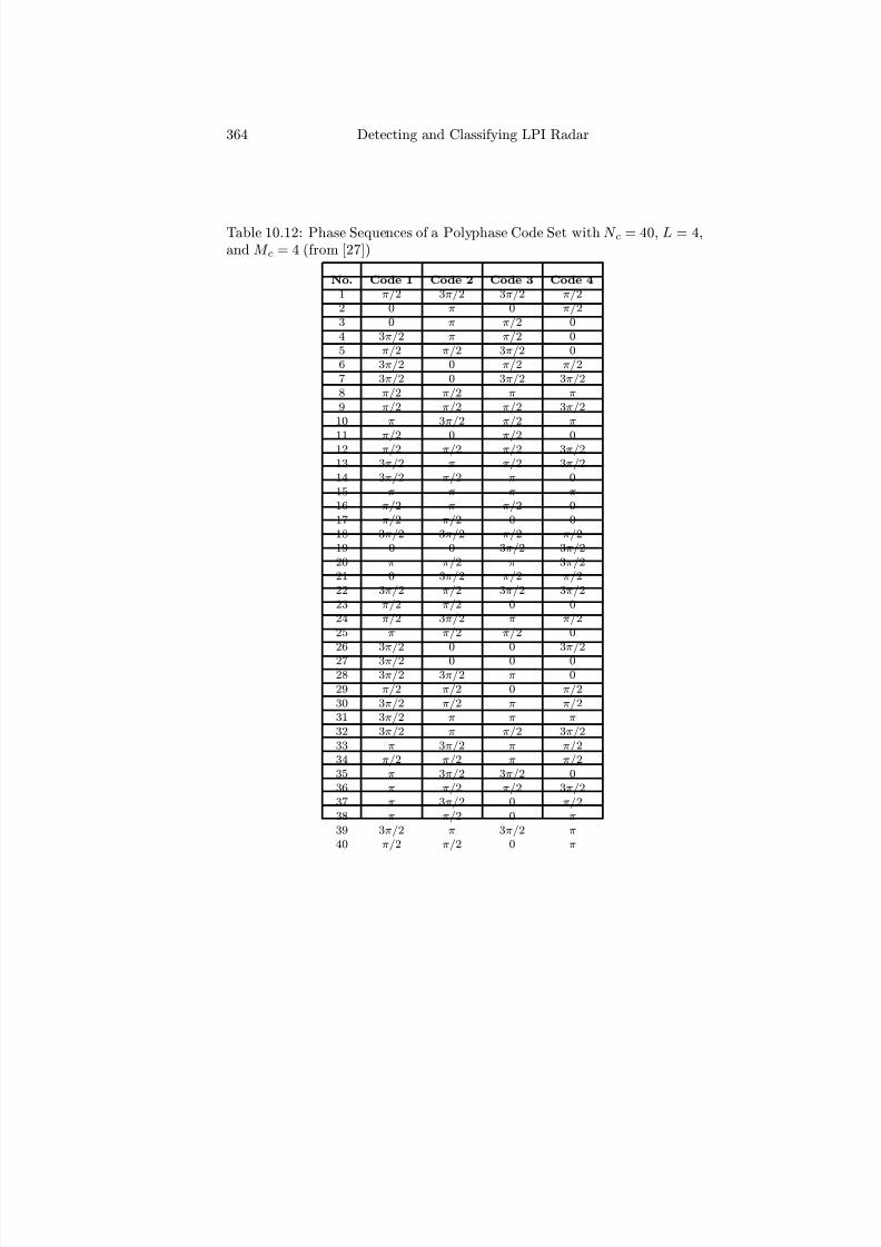
7/17/2019 1596932341 Intercept Radar.pdf
http://slidepdf.com/reader/full/1596932341-intercept-radarpdf 395/891
364 Detecting and Classifying LPI Radar
Table 10.12: Phase Sequences of a Polyphase Code Set with N c = 40, L = 4,and M c = 4 (from [27])
No. Code 1 Code 2 Code 3 Code 4
1 π/2 3π/2 3π/2 π/22 0 π 0 π/23 0 π π/2 04 3π/2 π π/2 05 π/2 π/2 3π/2 06 3π/2 0 π/2 π/27 3π/2 0 3π/2 3π/28 π/2 π/2 π π
9 π/2 π/2 π/2 3π/210 π 3π/2 π/2 π
11 π/2 0 π/2 012 π/2 π/2 π/2 3π/213 3π/2 π π/2 3π/214 3π/2 π/2 π 015 π π π π
16 π/2 π π/2 017 π/2 π/2 0 018 3π/2 3π/2 π/2 π/219 0 0 3π/2 3π/220 π π/2 π 3π/221 0 3π/2 π/2 π/222 3π/2 π/2 3π/2 3π/223 π/2 π/2 0 024 π/2 3π/2 π π/225 π π/2 π/2 026 3π/2 0 0 3π/227 3π/2 0 0 028 3π/2 3π/2 π 029 π/2 π/2 0 π/230 3π/2 π/2 π π/231 3π/2 π π π
32 3π/2 π π/2 3π/233 π 3π/2 π π/234 π/2 π/2 π π/235 π 3π/2 3π/2 036 π π/2 π/2 3π/237 π 3π/2 0 π/238 π π/2 0 π
39 3π/2 π 3π/2 π
40 π/2 π/2 0 π
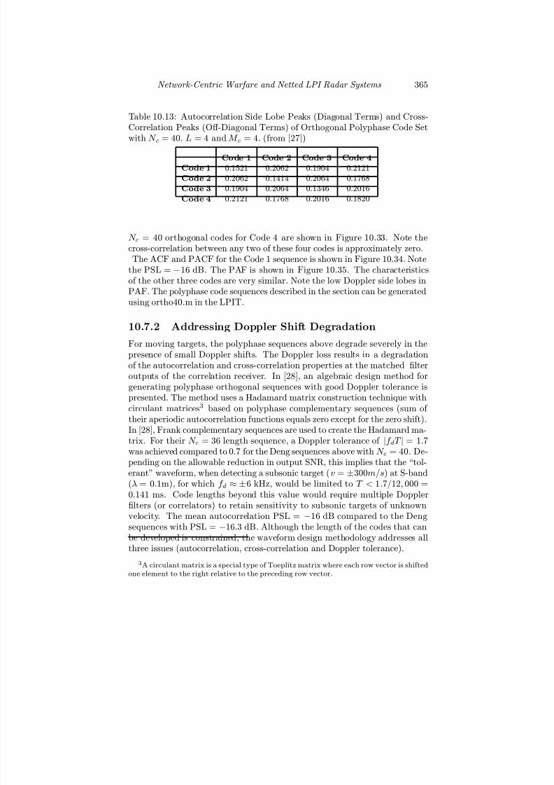
7/17/2019 1596932341 Intercept Radar.pdf
http://slidepdf.com/reader/full/1596932341-intercept-radarpdf 396/891
Network-Centric Warfare and Netted LPI Radar Systems 365
Table 10.13: Autocorrelation Side Lobe Peaks (Diagonal Terms) and Cross-Correlation Peaks (Off -Diagonal Terms) of Orthogonal Polyphase Code Set
with N c = 40, L = 4 and M c = 4. (from [27])
Co de 1 Code 2 Code 3 Code 4
Code 1 0.1521 0.2062 0.1904 0.2121
Code 2 0.2062 0.1414 0.2064 0.1768
Code 3 0.1904 0.2064 0.1346 0.2016
Code 4 0.2121 0.1768 0.2016 0.1820
N c = 40 orthogonal codes for Code 4 are shown in Figure 10.33. Note thecross-correlation between any two of these four codes is approximately zero.
The ACF and PACF for the Code 1 sequence is shown in Figure 10.34. Notethe PSL = −16 dB. The PAF is shown in Figure 10.35. The characteristicsof the other three codes are very similar. Note the low Doppler side lobes inPAF. The polyphase code sequences described in the section can be generatedusing ortho40.m in the LPIT.
10.7.2 Addressing Doppler Shift Degradation
For moving targets, the polyphase sequences above degrade severely in thepresence of small Doppler shifts. The Doppler loss results in a degradationof the autocorrelation and cross-correlation properties at the matched filteroutputs of the correlation receiver. In [28], an algebraic design method forgenerating polyphase orthogonal sequences with good Doppler tolerance ispresented. The method uses a Hadamard matrix construction technique with
circulant matrices
3
based on polyphase complementary sequences (sum of their aperiodic autocorrelation functions equals zero except for the zero shift).In [28], Frank complementary sequences are used to create the Hadamard ma-trix. For their N c = 36 length sequence, a Doppler tolerance of |f dT | = 1.7was achieved compared to 0.7 for the Deng sequences above with N c = 40. De-pending on the allowable reduction in output SNR, this implies that the “tol-erant” waveform, when detecting a subsonic target (v = ±300m/s) at S-band(λ = 0.1m), for which f d ≈ ±6 kHz, would be limited to T < 1.7/12, 000 =0.141 ms. Code lengths beyond this value would require multiple Dopplerfilters (or correlators) to retain sensitivity to subsonic targets of unknownvelocity. The mean autocorrelation PSL = −16 dB compared to the Dengsequences with PSL = −16.3 dB. Although the length of the codes that canbe developed is constrained, the waveform design methodology addresses all
three issues (autocorrelation, cross-correlation and Doppler tolerance).3A circulant matrix is a special type of Toeplitz matrix where each row vector is shifted
one element to the right relative to the preceding row vector.

7/17/2019 1596932341 Intercept Radar.pdf
http://slidepdf.com/reader/full/1596932341-intercept-radarpdf 397/891
366 Detecting and Classifying LPI Radar
Figure 10.29: Power spectrum magnitude of Code 1 with f c = 1,000 Hz.
Figure 10.30: Orthogonal polyphase shifts for Code 1 N c = 40 phase shifts.

7/17/2019 1596932341 Intercept Radar.pdf
http://slidepdf.com/reader/full/1596932341-intercept-radarpdf 398/891
Network-Centric Warfare and Netted LPI Radar Systems 367
Figure 10.31: Orthogonal polyphase shifts for Code 2 N c = 40 phase shifts.
Figure 10.32: Orthogonal polyphase shifts for Code 3 N c = 40 phase shifts.

7/17/2019 1596932341 Intercept Radar.pdf
http://slidepdf.com/reader/full/1596932341-intercept-radarpdf 399/891
368 Detecting and Classifying LPI Radar
Figure 10.33: Orthogonal polyphase shifts for Code 4 N c = 40 phase shifts.
Figure 10.34: Orthogonal polyphase Code 1 ACF and PACF.

7/17/2019 1596932341 Intercept Radar.pdf
http://slidepdf.com/reader/full/1596932341-intercept-radarpdf 400/891
Network-Centric Warfare and Netted LPI Radar Systems 369
Figure 10.35: Orthogonal polyphase Code 1 PAF.
In [29], a new set of polyphase sequences is presented with good corre-lation properties as well as resilience to Doppler shifts. The sequences arebuilt using a numerical cross entropy optimization based on correlation prop-erties and a structural constraint is also imposed on the optimized polyphasesequences so that Doppler tolerance is maintained. Deng [27] suggested im-proving Doppler tolerance by using an ambiguity based optimization costfunction to include reciprocals for the main lobe peaks, side lobe peaks andthe cross-correlation peaks for all possible Doppler frequencies. This methodhowever, is computationally costly for even short code lengths.
As another method, recall the polyphase code sets described inChapter 5 of Frank, P1—P4. For these codes, there is a harmonic relationshipof phases from one sequence element to the next that aids in the ability of the code to resist the Doppler loss. In [29], an algorithm is described wherethis harmonically related structure is applied as a constraint and added tothe correlation cross-entropy optimization algorithm to improve the Dopplertolerance. The technique can be used to construct arbitrary length sequencesfor an arbitrary number of transmitters. Table 10.14 lists three polyphasesequences of length N c = 40. Table 10.15 shows the autocorrelation PSLs
and cross-correlation peaks for these sequences. The mean PSL for these se-quences is −17.3 dB and the mean cross-correlation is −14.3 dB; these figuresimprove on the Deng sequences of the same length discussed above. The op-
7/17/2019 1596932341 Intercept Radar.pdf
http://slidepdf.com/reader/full/1596932341-intercept-radarpdf 401/891
370 Detecting and Classifying LPI Radar
timized polyphase code sequences described in the section can be generatedusing ortho40CE.m in the LPIT.
10.7.3 Orthogonal Frequency Hopping Sequences
Due to the flexible locations of the multitransmitters and multireceivers, thenetted radar system of systems has much stronger capability in target de-tection, tracking, recognition and electronic protection compared with theconventional emitter. In Chapter 6, an algebraic method was presented toderive a single discrete frequency-coding Costas sequence with N F frequenciesfor use in a monostatic frequency hopping LPI emitter. Although the Costasarrays have nearly an ideal periodic autocorrelation property, for any two ormore constructed Costas arrays there is no guarantee that any two sequenceswill have a nearly zero cross-correlation property.
In [30], a set of N F discrete frequency hopping waveforms with good auto-correlation and nearly zero cross-correlation were derived by using a numericaloptimization technique. In this technique, the result is achieved through min-imizing a cost function that measures the degree to which a result satisfies thedesign requirements. In frequency hopping waveform design, the cost functionis chosen as in the previous section as the sum of the total autocorrelationside lobe energy for each waveform in the set and the total cross-correlationenergy for all distinct combinations of two waveforms s p(t), sq(t) in the set.Thus, the cost function to be minimized for the discrete frequency hoppingwaveform design is
E =Ll=1
τ
|A(sl, τ )|2 +
L−1 p=1
Lq= p+1
τ
|C (s p, sq, τ )|2dτ (10.47)
Details on the minimization algorithm can be found in [30]. Table 10.16 liststhe three frequency hopping sequences of the designed waveform set withN F = 32 and L = 3. The autocorrelation side lobe peaks and cross-correlationpeaks of the designed frequency hopping sequence sets inTable 10.16 are given in Table 10.17.
The discrete frequency hopping sequence Code 1 was generated with abase frequency multiplier of 1,000 Hz. The N F = 32 codes were sampledwith f s = 100 kHz with t p = 0.001 s. The power spectrum magnitude of the discrete frequency hopping sequence Code 1 is shown in Figure 10.36.The ACF and the PACF are shown in Figure 10.37 and the PAF is shown inFigure 10.38. Note the extremely well behaved time and Doppler side lobelevels. The PSL = −20 dB. The discrete frequency coding waveforms can begenerated using dfc32.m in the LPIT.

7/17/2019 1596932341 Intercept Radar.pdf
http://slidepdf.com/reader/full/1596932341-intercept-radarpdf 402/891
Network-Centric Warfare and Netted LPI Radar Systems 371
Table 10.14: Optimized Cross-Entropy Sequences with N c = 40 (from [29])
No. Code 1 Code 2 Code 3
1 8π/5 3π/5 4π/5
2 π π/5 2π/5
3 6π/5 π 04 4π/5 6π/5 0
5 9π/5 9π/5 π
6 2π/5 9π/5 9π/57 27π/20 3π/20 21π/20
8 21π/20 3π/5 9π/20
9 3π/10 27π/20 6π/5
10 3π/20 3π/10 9π/2011 27π/20 27π/20 21π/20
12 27π/20 6π/5 27π/20
13 π/5 π/2 4π/514 0 4π/5 9π/10
15 π/10 π/2 π/10
16 4π/5 0 π/517 0 7π/10 9π/10
18 3π/5 4π/5 9π/10
19 π/20 0 0
20 π/5 π/20 π/2021 π/20 π/10 π/20
22 π/4 π/20 π/4
23 9π/10 4π/5 024 9π/10 π/10 9π/10
25 π/5 4π/5 0
26 7π/10 π/10 4π/527 0 9π/10 4π/5
28 π/5 3π/5 π/5
29 6π/5 6π/5 27π/20
30 27π/20 9π/20 3π/2031 0 9π/20 27π/20
32 0 0 27π/20
33 6π/5 27π/20 3π/1034 3π/10 6π/5 3π/4
35 7π/5 2π/5 6π/536 3π/5 6π/5 3π/5
37 π/5 7π/5 3π/5
38 6π/5 3π/5 6π/5
39 6π/5 0 7π/5
40 8π/5 9π/5 7π/5

7/17/2019 1596932341 Intercept Radar.pdf
http://slidepdf.com/reader/full/1596932341-intercept-radarpdf 403/891
372 Detecting and Classifying LPI Radar
Table 10.15: Autocorrelation Side Lobe Peaks (Diagonal Terms) and Cross-
Correlation Peaks (Off
-Diagonal Terms) for the Cross Entropy Sequence Setof Length N c = 40 (from [29])
Code 1 Code 2 Code 3
Code 1 0.1365 0.1820 0.1799
Code 2 0.1820 0.1303 0.1840
Code 3 0.1799 0.1840 0.1413
Table 10.16: Discrete Frequency Hopping Sequences with N F = 32 and L = 3(from [30])
No. Code 1 Code 2 Code 3
1 31 2 312 28 11 133 1 12 184 30 14 205 3 29 116 8 16 77 10 6 298 12 1 279 7 9 8
10 25 21 2211 11 24 012 15 23 113 23 5 2114 13 26 1415 27 19 9
16 22 3 1717 26 7 518 17 30 2519 5 13 2620 21 8 1021 6 20 1922 2 17 1623 29 18 3024 14 4 1525 16 0 1226 19 28 2327 9 31 428 20 15 329 18 27 630 0 10 2
31 24 25 2832 4 22 24

7/17/2019 1596932341 Intercept Radar.pdf
http://slidepdf.com/reader/full/1596932341-intercept-radarpdf 404/891
Network-Centric Warfare and Netted LPI Radar Systems 373
Table 10.17: Autocorrelation Side Lobe Peaks and Cross-Correlation Peaksof the Discrete Frequency Hopping Sequences in Table 10.16 (from [30])
Code 1 Code 2 Co de 3
Code 1 0.0764 0.0979 0.1250
Code 2 0.0979 0.0881 0.1068
Code 3 0.1250 0.1068 0.0855
Figure 10.36: Power spectrum magnitude of the orthogonal discrete frequencyhopping Code 1 with f s = 100 kHz.

7/17/2019 1596932341 Intercept Radar.pdf
http://slidepdf.com/reader/full/1596932341-intercept-radarpdf 405/891
374 Detecting and Classifying LPI Radar
Figure 10.37: ACF and PACF of the orthogonal discrete frequency hoppingCode 1 with f s = 100 kHz.
10.7.4 Noise Waveforms
The concept of a multiuser, wireless netted LPI radar system using randomnoise is proposed in [31]. The proposed system uses noise signals for radarsurveillance and a multiradar communication network for transferring thesensor data to a central command center where informed decisions can bemade. Due to the spectral characteristics of the UWB random noise wave-form, an LPI capability is provided while also efficiently sharing the frequencyspectrum with other users. A number of UWB random noise radar systemscan operate over the same frequency band with minimal cross-interferencesince each transmitted noise waveform is uncorrelated with the others. Itis this property that allows a number of the UWB noise radars to be inte-grated into a NCW architecture [31]. The bandlimited noise (1—2 GHz) is
also notch filtered (1.2—1.3 GHz) to provide room for the intrasensor networkcommunications among the diff erent emitters. The spectral fragmentationfor the embedded communication causes no distortion if the gap in the noise

7/17/2019 1596932341 Intercept Radar.pdf
http://slidepdf.com/reader/full/1596932341-intercept-radarpdf 406/891
Network-Centric Warfare and Netted LPI Radar Systems 375
Figure 10.38: PAF of the orthogonal discrete frequency hopping Code 1 withf s = 100 kHz.

7/17/2019 1596932341 Intercept Radar.pdf
http://slidepdf.com/reader/full/1596932341-intercept-radarpdf 407/891
376 Detecting and Classifying LPI Radar
Figure 10.39: Noise radar concept with (a) element-space approach and(b) beam-space approach (after [32]).
band is not excessive (≤ 30%). The sensor data to be shared is modulatedonto a CW signal whose frequency lies within the notch of the UWB noisesignal. Orthogonal frequency division multiple access modulation is used fortransporting the target data between sensors.
The development of a netted noise radar is also presented in [32]. Twotransmission approaches are compared as shown in Figure 10.39. The firstapproach shown in Figure 10.39(a), is the element space approach where mul-tiple channels (antennas) of independent noise are transmitted. K incoherentnoise sources are transmitted. Ignoring the angular variation in the target’sRCS, the received power is independent of the angle of the scatterer fromthe transmit array. The second approach shown in Figure 10.39(b), is thebeam-space approach where each independent noise source is fed into eachantenna but is delayed τ i (or phase shifted) so as to form a beam illuminat-ing a selected sector of the radar field of view (FOV). This eff ectively codeseach sector in the FOV according to a particular noise source. The direc-tion of each sector is determined by the delay (or phase shift) and the widthis determined by the beamwidth of the array. Comparison of element- and
beam-space approaches to the netted noise radar indicate that when oper-ating the transmit array at frequencies such that d/λ < 0.5 where d is thereceiver spacing, the beam-space approach is a more efficient method of con-

7/17/2019 1596932341 Intercept Radar.pdf
http://slidepdf.com/reader/full/1596932341-intercept-radarpdf 408/891
Network-Centric Warfare and Netted LPI Radar Systems 377
centrating the wave number spectrum of the transmit signal in the radiatingregion and minimizes the problem of nonradiating waves.
10.8 Netted Over-the-Horizon Radar Systems
Future OTHR systems are expected to deliver dramatically improved capa-bility in every performance dimension including LPI. There are three directbenefits to applying MIMO radar concepts to OTHR [33]. First it providesa means to implement radar management trade-off s between radar sensitiv-ity and surveillance footprint coverage allowing a more efficient use of re-sources (surveillance area requirements, sensitivity, target dynamic behavior,and the interaction of the target characteristics with the data processing al-gorithms). MIMO radar is also a convenient method to implement adaptiveprocessing algorithms on transmit for clutter mitigation. By changing theillumination source at the transmit array, the clutter is more eff ectively sup-
pressed. Consequently, orthogonal waveforms have also found application innetted OTHR systems [33]. The use of multiple simultaneously transmittedorthogonal waveforms permit better sensitivity and more flexible trade-off sin footprint coverage. It also allows for adaptive management of the trans-mitted beam to minimize clutter and simplifies propagation mode selectionfor improved clutter rejection.
In an OTHR, both the transmitter and receiver subsystems can be con-sidered as M and N dimensional digital arrays. The transmit subsystemconsists of one waveform generator per transmit power amplifier and trans-mit antenna element. The receive subsystem consists of one digitizing receiverper array element. Achieving full orthogonality with the CW waveform setover the space-time ambiguity of concern is not possible. Space-time adaptiveprocessing using multiple transmitters and receivers allows using one wave-form generator per transmit element and enabling the transmit and receivebeamforming to be performed entirely at the receive site [34]. The diversityof target scattering leads to better detection performance using lower powerwaveforms.
Orthogonal waveforms that can be used in OTHR include time-staggeredFMCW, Doppler off set FMCW and noise waveforms. The time-staggered
FMCW uses a time off set between diff erent FMCW waveforms to exploit thefact that the range interval of interest is frequently limited by ionosphericpropagation. In surface modes (high Doppler resolution mode), low WRFsare used over extended CITs. It is therefore possible to provide orthogo-nality between a number of waveforms after range correlation with a singlereference waveform. The approach maintains the attractive power efficiency
and spectral occupancy of the FMCW waveform. For the Doppler o ff set FMCW a small frequency off set between FMCW waveforms provides orthog-onality after slow-time Doppler processing (slow-time MIMO). In this case,

7/17/2019 1596932341 Intercept Radar.pdf
http://slidepdf.com/reader/full/1596932341-intercept-radarpdf 409/891
378 Detecting and Classifying LPI Radar
the Doppler extent of the clutter and expected target Doppler shifts limitthe number of concurrent orthogonal waveforms that can be supported. Thiswaveform approach is more appropriate to the air-mode for aircraft detection.The band-limited noise waveforms also provide an orthogonal waveform choicedespite the large peak to average power ratio and poor Doppler sensitivity.This approach provides a broad class of orthogonal waveforms.
References
[1] Cebrowski, A. K., “Implementation of Network-Centric Warfare,” Office of Force Transformation, 2004.
[2] Ahmed, A. A., Hongchi, S., and Shang, Y., “A survey on network protocolsfor wireless sensor networks,” Proc. of the IEEE International Conf. on
Information Technology: Research and Education , pp. 301—305, Aug. 2003.
[3] Karlof, C. and Wagner, D., “Secure routing in wireless sensor networks: at-
tacks and countermeasures,” Proc. of the IEEE International Workshop on Sensor Network Protocols and Applications , pp. 113—127, 2003.
[4] Stein, F., Garska, J., and McIndoo, P.L., “Network-centric warfare: Impacton Army operations,” EUROCOMM 2000 Information Systems for Enhanced
Public Safety and Security , IEEE/AFCEA, pp. 288—295, 2000.
[5] Kruse, J., Adkins, M. and Holloman, K. A., “Network centric warfare in theU.S. Navy’s fifth fleet,” Proc. of the IEEE 38th Hawaii International Conf.
on Systems Sciences , 2005.
[6] Chen, Y-Q, and Pace, P. E., “Simulation of Information Metrics to Assessthe Value of Networking in a General Battlespace Topology,” Proc. of the
IEEE International Conf. on System of Systems Engineering , June 2008.
[7] Boyd, J.R., “A discourse on winning and losing,” Title Boyd gave to his
collection of briefings on competitive strategy (widely known as the “GreenBook,” with apologies to Wittgenstein), 1987.
[8] Ling, F.M., Moon, T., and Kruzins, E., “Proposed network centric warfaremetrics: From connectivity to the OODA cycle,” Military Operations Re-
search , vol. 10 No. 1, pp. 5—13, 2005.
[9] Shannon, C. E., “A mathematical theory of communication,” Bell Systems
Technical Journal , July 1948.
[10] Phister, P.W. Jr., and Cherry, J.D., “Command and control concepts withinthe network-centric operations construct,” Proc. of the IEEE Aerospace
Conf., pp. 1—9, Mar. 4—11, 2006.
[11] Posiel, R. Modern Communications Jamming Principles and Techniques , ArtechHouse Inc., 2004.
[12] Hume, A. L. and Baker, C. J., “Netted radar sensing,” Proc. of the CIE International Conf. on Radar , pp. 110—114, Oct. 2001.

7/17/2019 1596932341 Intercept Radar.pdf
http://slidepdf.com/reader/full/1596932341-intercept-radarpdf 410/891
Network-Centric Warfare and Netted LPI Radar Systems 379
[13] Teng, Y., Griffiths, H. D., Baker, C. J., Woodbridge, K., “Netted radar sen-sitivity and ambiguity,” IET Radar and Sonar Navig., Vol. 1, No. 6, pp.479—486, 2007.
[14] Derham, T.E., Doughty, S., Woodbridge, K., Baker, C.J., “Design and eval-uation of a low-cost multistatic netted radar system,” IET Radar, Sonar &
Navigation , Vol. 1, No. 5, pp. 362—368, October 2007.
[15] Lehmann N. H., Haimovich, A. M., Blum, R. S., and Cimini, L., “Highresolution capabilities of MIMO radar,” Record of the Fortieth Asilomar Conf.
on Signals, Systems and Computers , pp. 25—30, 2006.
[16] Bliss, D. W., and Forsythe, K. W., “Multiple-input multiple-output (MIMO)radar and imaging: degrees of freedom and resolution,” Record of the Thirty-
Seventh Asilomar Conf. on Signals, Systems and Computers , Vol. 1, pp.54—59, Nov., 2003.
[17] Sammartino, P.F., Baker, C.J., and Griffiths, H.D., “Target model eff ectson MIMO radar performance,” Proc. of the IEEE International Conf. on
Acoustics, Speech and Signal Processing , pp. V-1129—V-1132, May, 2006.[18] Haimovich, A. M., Blum, R. S., and Cimini, L. J. Jr., “MIMO radar with
widely separated antennas,” IEEE Signal Processing Magazine , pp. 116—129,Jan. 2008.
[19] Hume, A. L. and Baker, C. J., “Netted radar sensing,” Proc. of the IEEE
Radar Conf., pp. 23—26, 2001.
[20] Baker, C. J., and Hume, A. L., “Netted radar sensing,”IEEE Aerospace and
Electronic Systems Magazine , Vol. 18, No. 2, pp. 3—6, Feb. 2001.
[21] Fishler, E., Haimovich, A., Blum, R., Cimini, L. J., Chizhik, D., and Valen-zuela, R. A., “Spatial diversity in radars - models and detection performance,”IEEE Trans. of Signal Processing, Vol. 54, No. 3, pp. 823—838, 2006.
[22] Chen, C-Y, and Vaidyanathan, P. P., “Properties of the MIMO radar ambi-guity function,” Proc. of the IEEE International Conf. on Acoustics, Speech
and Signal Processing , pp. 2309—2312, 2008.
[23] Teng, Y., Baker, C. J., and Woodbridge, K., “Netted radar sensitivity andthe ambiguity function,” Proc. of the International Conf. on Radar , Vol. 1,No. 6, pp. 1—4, Dec. 2006.
[24] Papoutsis, I., Baker, C. J., and Griffiths, H. D., “Netted radar and the ambi-guity function,” Proc. of the IEEE International Radar Conf., pp. 883—888,2005.
[25] Li, J., Stoica, P., Xu, L., and Roberts, W., “On parameter identifiability of MIMO radar,” IEEE Signal Processing Letters, Vol. 14, No. 12, pp. 968—971,Dec. 2007.
[26] Chen, Y-Q, and Pace, P. E., “Simulation of Network-Enabled Radar Systemsto Assess the Value of Jamming in a General Radar Topology,” Proc. of the
IEEE International Conf. on System of Systems Engineering , June 2008.[27] Deng, H., “Polyphase code design for orthogonal netted radar,” IEEE Trans.
on Signal Processing, Vol. 52, No. 11, pp. 3126—3135, Nov. 2004.
7/17/2019 1596932341 Intercept Radar.pdf
http://slidepdf.com/reader/full/1596932341-intercept-radarpdf 411/891
380 Detecting and Classifying LPI Radar
[28] Khan, H. A., and Edwards, D. J., “Doppler problems in orthogonal MIMOradars,” Proc. of the IEEE Conf. on Radar , pp. 244—247, 2006.
[29] Khan, H. A., Zhang, Y., Ji, C. Stevens, C. J., Edwards, D. J., and O’Brien, D.,“Optimizing polyphase sequences for orthogonal netted radar,” IEEE Signal
Processing Letters , Vol. 13, No. 10, pp. 589—592, 2006.
[30] Deng, H., “Discrete frequency-coding waveform design for netted radar sys-tems,” IEEE Signal Processing Letters, Vol. 11, No. 2, pp. 179—182, Feb.2004.
[31] Surender, S. C., and Narayanan, R. M., “Covert netted wireless noise radarsensor: OFDMA-based communication architecture,” Proc. of the Military
Communications Conf., pp. 1—7, Oct. 2002.
[32] Gray, D. A., and Fry, R., “MIMO noise radar—element and beam space com-parisons,” Proc. IEEE Waveform Diversity & Design Conf., pp. 344—347,2007.
[33] Frazer, G. J., Johnson, B. A., Abramovich, Y. I., “Orthogonal waveform
support in MIMO HF OTH radars,” Proc. IEEE Waveform Diversity & Design Conf., pp. 423—427, 2007.
[34] Frazer, G. J., Abramovich, Y. I., and Johnson, B. A., “Spatially waveformdiverse radar: perspectives for high frequency OTHR,” Proc. IEEE Radar
Conf., pp. 385—390, April 2007.
Problems
1. A netted LPI radar transmits the target parameters using −1.0 and 0.0-V levels with a probability of 0.2 each and 3.0- and 4.0-V levels with aprobability of 0.3 each. Determine the average information being sent.
2. A C2 operator uses a numerical keypad that has the digits 0, 1, 2, 3,4, 5, 6, 7, 8, and 9. Assume that the probability of sending any onedigit is the same as that for sending any of the other digits. Calculatehow often the operator must press the buttons in order to send outinformation at the rate of 2 bits/s.
3. An army field computer has 110 characters on the keyboard and eachcharacter is sent using binary words. (a) What is the number of bitsrequired to represent each character? (b) How fast can the charactersbe sent (characters/s) over a channel if the channel bandwidth is 3.2kHz and the SNR=20 dB? (c) What is the entropy of each character if each is equally likely to be sent?
4. A 480-by-500 pixel range-Doppler image is to be transmitted from a
netted LPI radar where each pixel can have one of 32 intensity values.The emitter sends 30 images/s. If all image elements are assumed tobe independent and all 32 intensity levels are assumed to be equally

7/17/2019 1596932341 Intercept Radar.pdf
http://slidepdf.com/reader/full/1596932341-intercept-radarpdf 412/891
Network-Centric Warfare and Netted LPI Radar Systems 381
Figure 10.40: Destruction of terrorist weapon system.
likely, (a) determine the source rate λ in (bits/s). (b) If the image is tobe transmitted over a channel with a 4.5-MHz bandwidth and a 35-dBSNR, find the capacity of the channel (bits/s).
5. The USS Enterprise (capability K = 1.0) has launched a Tomahawkmissile to destroy a terrorist weapon system as shown Figure 10.40. To
follow up with a damage report, a predator UAV follows the Tomahawk.To provide an intelligence, surveillance and reconnaissance (ISR) com-ponent, a Global Hawk (K = 0.8) is also used. The Tomahawk missilecapability is given as K = 0.3 due to its limited connectivity and signalrerouting options (note its unidirectional link to the Global Hawk). ThePredator also has a limited signal rerouting capability and is given thecapability value K = 0.5. Consider each link to have a flow componentand value component of either 1 or zero (i.e., F = L = 1, 0). (a) Findthe reference connectivity measure C RM . (b) Determine the networkreach I R. (c) Determine the network reach if a jammer takes out thelink between the USS Enterprise and the Tomahawk. (d) To examinethe impact of the rerouting options of the original network configura-tion (unjammed), let each node capability be K = 1.0 and determinethe network reach.
7/17/2019 1596932341 Intercept Radar.pdf
http://slidepdf.com/reader/full/1596932341-intercept-radarpdf 413/891
382 Detecting and Classifying LPI Radar
6. Consider problem 5. (a) If the rate that information is processed bynode μ = 1 is λ1 = 50 kHz, node μ = 2 is λ2 = 18 kHz, node μ =3 is λ3 = 260 kHz, and node μ = 4 is λ4 = 3 kHz, determine thenetwork richness RQ (average rate that knowledge is generated throughthe network). (b) Using the network richness calculated in Problem 5above, determine the network’s characteristic tempo λT . (c) Considerthat the command and control (C2) decision making speed to targetthe Tomahawk missile is λC 2 = 0.5 kHz. After the decision is made, ittakes 0.5 ms to send the retargeting command to the missile (η1 = 2kHz). After the missile receives the retargeting command, the missileguidance takes 0.25 ms to initiate the turn (η2 = 4 kHz). Calculate theOODA operational tempo ΛOODA for this retargeting command.
7. Behavior of the OODA tempo: The action tempos of a force will varyvastly depending on the specific net-centric EW situation; it is notpossible to make general statements about their scale. Therefore, theaction tempos can be treated as adjustable parameters in ΛOODA. Toillustrate the behavior of the OODA tempo with respect to the networktempo, we can normalize both by the C2 tempo. Using MATLAB,plot on the same graph the ΛOODA/λC 2 (vertical axis) versus λT /λC 2(horizontal axis) for the three action tempos: (a) η1 = 0.5λC 2 andη2 = 0.25λC 2 (low-action tempo), (b) η1 = λC 2 and η2 = λC 2 (medium-action tempo), and (c) η1 = 2λC 2 and η2 = 4λC 2 (high-action tempo).What can you conclude about the OODA tempo and the C2 tempo asthe network tempo increases?
8. Using the LPIsimNet tools (a) complete the tutorial in Appendix D forthe sensor network analysis and the netted radar analysis. (b) Constructa sensor network with four nodes, and a jammer. Movement of one or
more nodes should be included with five time index steps. Build ananalysis summary of the results. (c) Construct corresponding nettedradar scenario with four LPI emitters, a target and a jammer. Buildan analysis summary of the results. (d) What insights are you able togather from your simulation study?
9. (a) Add to the LPIT, four CW orthogonal PSK signals each with oneof the polyphase codes shown in Table 10.12. Include five periods of thecode set for each signal. (b) Generate the four polyphase signals withf c = 1 kHz, and B = 500 Hz. (c) Compute the ACF, PACF and PAFof each signal with N = 1 and N = 3. (d) How do the PSL levels of theorthogonal PSK waveforms compare with the polyphase codes Frank,P1—P4 ? (e) Compute the cross-correlation of the four PSK signals to
verify Table 10.13.

7/17/2019 1596932341 Intercept Radar.pdf
http://slidepdf.com/reader/full/1596932341-intercept-radarpdf 414/891
Network-Centric Warfare and Netted LPI Radar Systems 383
10. (a) Repeat the problem above for the cross-entropy orthogonal sequencesgiven in Table 10.14 with correlation properties given inTable 10.15. (b) Repeat for the discrete frequency hopping sequencesgiven in Table 10.16 and correlation properties given in Table 10.17using a scale factor of 102 Hz.

7/17/2019 1596932341 Intercept Radar.pdf
http://slidepdf.com/reader/full/1596932341-intercept-radarpdf 415/891

7/17/2019 1596932341 Intercept Radar.pdf
http://slidepdf.com/reader/full/1596932341-intercept-radarpdf 416/891
PART II:
INTERCEPT RECEIVER STRATEGIES AND
SIGNAL PROCESSING

7/17/2019 1596932341 Intercept Radar.pdf
http://slidepdf.com/reader/full/1596932341-intercept-radarpdf 417/891

7/17/2019 1596932341 Intercept Radar.pdf
http://slidepdf.com/reader/full/1596932341-intercept-radarpdf 418/891
Chapter 11
Strategies for Intercepting
LPI Radar Signals
The LPI radar characteristics discussed in the first part of this book (Chap-ters 1—10) pose a particular challenge to the noncooperative intercept receiver.Modern electronic warfare (EW) intercept receivers must perform the tasksof detection, parameter identification, classification, and exploitation in acomplex environment of high noise interference and multiple signals. Thewideband nature of the LPI emitter signal can force the intercept receiverto have a significant processing gain by implementing sophisticated receiverarchitectures and signal processing algorithms (time-frequency, bifrequency)in order to determine the waveform parameters. In this chapter, modernnetwork-centric strategies for EW receiver architectures are discussed, anda contrast is drawn to the traditional platform-centric approach. This in-cludes the use of swarm intelligence. In addition, the look-through problemis discussed in the framework of suppression of enemy defense. Digital re-ceiver architectures are briefly discussed including the direct RF samplingapproach. EW intercept receiver problems are also emphasized.
11.1 EW Intercept Receiver Techniques
11.1.1 Traditional Approach
Electronic warfare intercept receivers are used to process threats on the mod-
ern electronic battlefield, and consequently, must cover extremely wide bandsfrom 300 MHz to 100 GHz and above, since they do not know the charac-teristics of the signal that they are attempting to intercept. The widebandnature of LPI threat signals presents a significant challenge to the intercept
387
7/17/2019 1596932341 Intercept Radar.pdf
http://slidepdf.com/reader/full/1596932341-intercept-radarpdf 419/891
388 Detecting and Classifying LPI Radar
receiver design. The interception of LPI radar signals has been a topic of investigation for over a decade [1—3]. Traditionally, EW receivers have beendivided into three categories: radar warning receivers, electronic support re-ceivers, and electronic intelligence receivers. RWRs are designed to passivelyintercept enemy radars in time to enable the pilot to react quickly throughmaneuvering or employing appropriate electronic attack techniques. Theiruse on the battlefield is time-critical, and combat action is taken directlyfrom their threat information output. Electronic support receivers encom-pass all actions necessary to provide the information required for immediatedecisions involving EW operations, threat avoidance, targeting, and homing.Although not as time-critical as RWRs, information operations rely heavilyon ES receivers for intelligence updates and important operational decisions.
For electronic intelligence receivers, the information provided is extractedfrom detailed analysis of radar signals and other noncommunication emit-ters in a timely manner. Although their operation is the least time critical,their threat identification is used to update national databases. Examplesof U.S. collection ELINT assets include the U2 Senior Ruby, the Army’sGuard Rail, and the Air Force’s RC-135 Rivet Joint. These high-value stand-off assets typically operate hundreds of kilometers from the emitter and ata high altitude. Together, these receivers provide the underlying intelligenceneeded for weapon systems deployment. In a platform-centric configuration,each weapon system traditionally had its own receiver system and, if thatreceiver was remote, there was a stovepipe communication system providingthe intercept data back to the shooter.
There are limitations to the use of intercept receivers in a platform-centric
confi
guration. Geometrical limitations include extended stand-off
ranges andalignment problems, which make it especially difficult to detect and jam LPIemitters. Also, the intercept receiver is limited by look-through . The look-through process allows the jammer to observe its eff ectiveness on the LPIemitter by stopping the jamming assignment to listen periodically. This re-sults in inefficient jammer management, and limited coordination during amission.
11.1.2 The Look-Through Problem
To emphasize the look-through problem, consider a frequency-hopping LPI airdefense radar used for targeting a surface-to-air missile (SAM) against an in-coming strike aircraft. To protect the strike aircraft against these SAM sites,
platforms such as the EA-6B Prowler provide standoff
(long-range) jammingof the enemy radar, in what is normally called a suppression of enemy air de-fense operation.1 The aircraft has a fully integrated electronic warfare systemcombining long-range, all-weather receive and jamming capabilities, mainly
1The EA-6B is also used to protect ground troops and ships, by jamming enemy elec-tronic data links and communications.
7/17/2019 1596932341 Intercept Radar.pdf
http://slidepdf.com/reader/full/1596932341-intercept-radarpdf 420/891
Strategies for Intercepting LPI Radar Signals 389
supplied by the Litton LR-700 intercept receiver, working together with theAN/ALQ-99 tactical jamming system (TJS). The Litton LR-700 is the newintercept receiver system in the Increased Capability III (ICAP III) versionof the EA-6B, and gives the Prowler a selective-reactive jamming capabilitywith the TJS. During a SEAD operation, the LR-700 receiver on board thesuppression aircraft must detect the threat emitters and manage the TJS inorder to prevent the radar from detecting the inbound strike aircraft it istrying to protect.
During the jamming process, a certain amount of look-through is required.For example, with an EA-6B reactively jamming a frequency-hopping radar,the jamming must stop in order to sense the radar’s transmit frequency. Of course, the duty cycle of the intercept receiver look-through process must beless than the time necessary for the radar to sense it is being jammed, andswitch frequencies. The bottom line is that any amount of look-through isnot desired, since this allows the threat radar a window in which to detectthe strike aircraft.
If however, the EA-6B integrates threat parameters from an electronicorder-of-battle database, a reconnaissance aircraft with near real-time on-scene intelligence collection, analysis, and dissemination capabilities (e.g.,Rivet Joint), and frequency data from an off -board stand-in sensor (e.g., aUAV) to cue the on-board intercept receiver (tip and tune), a fast reactiveelectronic attack can be performed that eliminates the need for look-through.For the reactive jamming assignments to be eff ective, however, the data linkused to provide the cueing data must not induce a delay time of any signifi-cance to the reactive assignment. That is, if the frequency-hopping radar can
switch frequencies faster than the cueing data can arrive from the off
-boardintercept receiver, then the eff ectiveness is significantly degraded.
11.1.3 Modern Network-Centric Concepts Arriving
Due to the complex emitter modulations now available, and the speed withwhich information is shared, the distinction between the roles of RWRs, ES,and ELINT receivers is fast disappearing, and all capabilities are being in-tegrated within a single EW receiver system, in order to provide a completesituational awareness for ships, helos, and high-value aircraft. In addition,these receivers must now include precision direction finding, countermeasurescontrol, cueing of weapon systems, enhanced radar warning, fusion of off -board sensors and databases, and full integration with the electronic combat
system. Other capabilities will include emitter classifi
cation and identifi
ca-tion, emitter-to-platform correlation, detailed analysis, and signal recording.Eliminating the limitations inherent in a platform-centric configuration
comes from a distributed system of systems. A distributed system of systemsprovides significant geometric flexibility, and can reduce or eliminate the needfor look-through. In addition, coordinated jammer responses and improved

7/17/2019 1596932341 Intercept Radar.pdf
http://slidepdf.com/reader/full/1596932341-intercept-radarpdf 421/891
390 Detecting and Classifying LPI Radar
Figure 11.1: Disabling an LPI emitter within a network-centric architecture.
jammer management can be achieved due to better information being avail-able. The ability for EW receivers to acquire, track, and locate conventionalthreat emitters and targets, and share this information among stand-off plat-forms (e.g., for weapons targeting), is an example of a network-centric archi-
tecture, and represents a fundamental shift from a platform-centric approach.As emphasized in Chapter 10, in a network-centric architecture, the net-
work acts as a force multiplier by networking sensors (e.g., EW receivers),decision makers, and shooters (e.g., weapons systems), to achieve sharedawareness. The network requires sufficient bandwidth for all users to takeadvantage of data mining in appropriate databases afloat and ashore. Thearchitecture is determined mostly by the mission altitudes, signal densities,reaction times, and modulation analysis that must be performed. Figure 11.1demonstrates the detection and jamming of an LPI emitter using a network-centric architecture. See also Figure 10.1 for comparison. The LPI emitteris detected using a number of sensors that relay the information to both acommand and control point, and the proper shooter. The command andcontrol then allows the shooter to apply the appropriate electronic attack to
disable the LPI emitter. The shooter also relays its information concerningthe jammed emitter back to both the sensors and the command and control.That is, instead of each platform making decisions on information received byonly its own intercept receiver (the platform-centric approach), modern EWreceivers integrate information from many sensors and databases for target-

7/17/2019 1596932341 Intercept Radar.pdf
http://slidepdf.com/reader/full/1596932341-intercept-radarpdf 422/891
Strategies for Intercepting LPI Radar Signals 391
Figure 11.2: Predator UAV with a Hellfire missile.
ing. Through a superior battlespace awareness, forces can employ the bestweapons on the right targets to greatly reduce risk to themselves, and increasethe opportunity for a successful LPI emitter engagement.
11.2 Detecting the LPI Radar with UAVs
The network-centric approach to intercept receiver integration is an importanttrend. This capability requires the platforms to be available in the correctlocation, and the data links between those platforms to be jam resistant. Un-
fortunately, LPI emitters are becoming increasingly diffi
cult to detect, locate,and track from stand-off platforms, due to their low peak power (< 1W),low side lobes (−40 dB down), short on-times (ms), high mobility, and use of terrain masking. As a result, the stand-off platforms with EW receivers areaugmented by specialized receivers that can go to the emitters (stand-in plat-forms). These specialized receivers are mounted, for example, in unmannedaerial vehicles such as the Predator, shown in Figure 11.2.
The use of swarm intelligence technology is fast becoming an importantconcept in network-centric sensor configurations. Swarm intelligence allowsthe design of EW receiver networks to detect LPI emitters, and is inspired bythe behavior of social insects [4]. In a swarm sensor architecture, the signalcollection capability is defined by the group behavior and not the individualbehavior. One advantage of using a UAV swarm of EW receivers is the
ability to behave autonomously, using digital information pheromones (DIPs;see page 106 in [4]). In what follows we use the analogy of the EW receiver asbeing an “ant” insect that exists within a swarm. The idea is to use anotherEW receiver’s (ant’s) experience in prior LPI emitter searches. For example,ants that are looking for particular LPI emitters, access information that hasbeen left in the form of DIPs (ratings) from previous detections by other

7/17/2019 1596932341 Intercept Radar.pdf
http://slidepdf.com/reader/full/1596932341-intercept-radarpdf 423/891
392 Detecting and Classifying LPI Radar
colony members. As LPI emitters are detected, an “ant DIP” is publishedon the network by this “ant server.” This lets other ants know how manyprevious detections of this emitter were found, and the characteristics of theemitter. Ant DIPs that are continuously detected are continually reinforced,while those that are disabled (see Figure 11.1) evaporate. Only informationthat is regularly verified and reinforced is conserved.
This type of behavior requires only a small number of operators to controlmany UAVs. Another advantage is the ability of the UAVs to behave coopera-tively. Cooperative behavior allows the UAVs to form a robust, self-organizingand self-adapting sensor architecture, while retaining the intercept functioneven in the presence of a loss. The swarm LPI detection architecture requiresonly low-cost medium-endurance airframes (expendable), existing widebandintercept receivers (e.g., R-300A, highly integrated microwave receiver), andthe use of swarm logic [4] with intraswarm communications, using, for ex-ample, an 802.11 link. With the swarm approach, LPI radars run the riskof detection (and classification), especially when the intercept receiver incor-porates advanced signal processing techniques that take advantage of time-frequency, bifrequency processing. According to the 2002 Defense AcquisitionBoard, EA from the UAV platform will become a significant capability.
11.3 Noncooperative Intercept Receivers
The EW community has long debated and ranked many diff erent interceptreceiver architectures based on their ability to process signals [5, 6]. Thecomparisons, however, have limited usefulness, since diff erent mission scenar-
ios require diff erent capabilities. What is certain, however, is that future EWreceivers will be digital, and will incorporate various technologies as discussedbelow.
11.3.1 Comparison of Classic Receiver Architectures for
Detecting LPI Waveforms
There are many variations of intercept receivers. These passive receivers canbe used to detect the LPI emitter emissions over considerable distances. Inthis section, three popular intercept receiver architectures are compared interms of their ability to detect several types of LPI emitter waveforms. Thereceivers that are compared include the square-law, wideband and channelizedreceivers [7]. These receivers are relatively inexpensive, readily accessible andare shown in Figure 11.3. The square-law receiver is an energy detector.
The parameters of the square-law receiver are given in Table 11.1. Thewideband crystal video receiver is characterized by a wide RF bandwidth toaccount for the uncertainty in the intercepted signal parameters. The spec-ifications of the wideband receiver are given in Table 11.2. The channelized

7/17/2019 1596932341 Intercept Radar.pdf
http://slidepdf.com/reader/full/1596932341-intercept-radarpdf 424/891
Strategies for Intercepting LPI Radar Signals 393
Figure 11.3: Block diagram of receiver architectures being compared with(a) square-law, (b) wideband crystal video, and (c) channelized.
Table 11.1: Square-Law Receiver Parameters [7]
Receiver Feature Specification
Noise figure 8 dBInstantaneous bandwidth 1 GHzNoise floor −76 dBmSystem loss 12 dBVideo bandwidth 60 kHzIntegration time period matchedDetection threshold SNR = 12 dBLocal oscillator 12 MHzIF bandwidth 12 MHz

7/17/2019 1596932341 Intercept Radar.pdf
http://slidepdf.com/reader/full/1596932341-intercept-radarpdf 425/891
394 Detecting and Classifying LPI Radar
Table 11.2: Wideband Crystal Receiver Parameters [7]
Receiver Feature Specification
Noise figure 8 dBInstantaneous bandwidth 4 GHzNoise floor −70 dBmSystem loss 10 dBVideo bandwidth 1 MHzIntegration time 100 nsDetection threshold SNR = 12 dBLocal oscillator f LO 12 MHz
Table 11.3: Channelized Receiver Parameters [7]
Receiver Feature Specification
Number of channels 40Noise figure 10 dBInstantaneous bandwidth 2 GHzChannel bandwidth 50 MHzNoise floor −92 dBmSystem loss 5 dBVideo bandwidth 1.25 MHz
Integration time 100 nsDetection threshold SNR = 12 dB
receiver contains a large number of parallel narrowband receivers. The RFband is divided into 40 contiguous front-end channels (N = 40). The channeloutputs are all folded into a common baseband and passed through 40 IFsubchannels (M = 40). The folding is done with the local oscillators at 50MHz frequency increments. The 40 RF channels span 2 GHz and each chan-nel is 50 MHz wide. The 40 IF subchannels each span 1.25 MHz giving a final50 MHz coverage of the spectrum. The parameters for the channelized re-ceiver are shown in Table 11.3.
LPI Waveforms Used
To compare each receiver’s detectability performance, it is important that theemitter waveforms have equal bandwidth and equal energy. This is becausemany of the compression waveforms off er the same range resolution but not
7/17/2019 1596932341 Intercept Radar.pdf
http://slidepdf.com/reader/full/1596932341-intercept-radarpdf 426/891
Strategies for Intercepting LPI Radar Signals 395
all have the same LPI/LPID properties [8]. Six waveforms were comparedincluding a rectangular pulse, an FMCW, P1, P2, P3 and P4 all with arange resolution of 50m. The polyphase codes each have a subcode period of tb = 333 ns (B = 3 MHz) and a code period of T = 64tb = 21.3 μs. TheFMCW has a modulation period tm = 64tb or 21.3 μs and the modulationbandwidth is ∆F = 3 MHz (starting at dc). The rectangular pulse has a pulseduration τ R = tb = 333 ns with a pulse repetition interval PRI = 64 tb = 21.3μs. The average power transmitted by each emitter is P CW = 100W andλ = 3 × 10⁻²m. The emitter transmit antenna gain in the direction of theintercept receiver is Gr = 0 dB [8].
Intercept Range and Sensitivity Comparison
A MATLAB simulation was run first to determine the sensitivity. The sen-sitivity δ I is the minimum signal at the back end of the receiver that isdetectable given the noise floor associated with that particular receiver. Thesensitivity was determined by iteratively adjusting the front-end signal am-plitude that achieves the required back-end SNR. Since the noise floor, noisefigure, bandwidths and integration times are defined for each receiver, theamplitude was adjusted until detection was achieved [8].
Models were developed in MATLAB for each receiver in order to find thefront-end signal strength necessary to satisfy the minimum back-end SNR.A voltage gain of 20 dB was used for each receiver. After determining thesensitivity for each receiver, the intercept range (direct path) was calculatedfrom (1.41) as
RI max = λ
4π P CW GtGI
δ I (11.1)
where LRT = LIR = L1 = 1. Also, the propagation loss was assumed tobe zero. Each receiver uses a 12-dB detection threshold. In the case of thechannelized receiver, the detection threshold applies to each channel. Bykeeping the threshold the same across all receivers, the relative detectioncapability can be quantified. A 1-hour false alarm interval was assumed foreach receiver and for each channel of the channelized receiver. The sensitivityand interception range for each intercept receiver is given in Table 11.4.
The square-law detector was most eff ective and detected all signals atessentially the same range (≈ 25 km). The least eff ective receiver was thewideband receiver. The most detectable waveform in the wideband and chan-nelized receiver was the rectangular pulse. The P1, P2 and P4 perform signif-
icantly better than the rectangular pulse, P3 and FMCW in the channelizedreceiver. The P2 waveform represents a factor of 2.3 reduction in range overthe rectangular pulse in the channelized receiver [8].
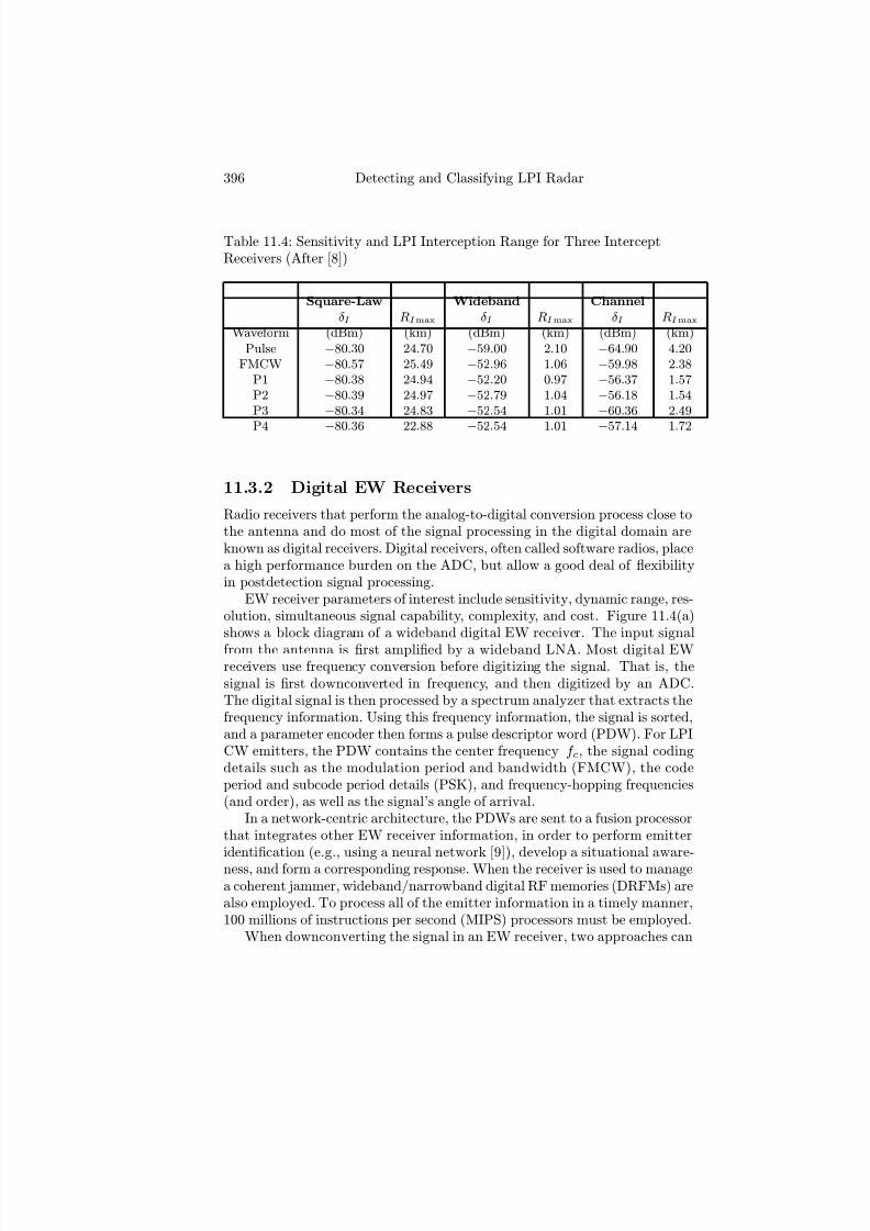
7/17/2019 1596932341 Intercept Radar.pdf
http://slidepdf.com/reader/full/1596932341-intercept-radarpdf 427/891
396 Detecting and Classifying LPI Radar
Table 11.4: Sensitivity and LPI Interception Range for Three InterceptReceivers (After [8])
Square-Law Wideband Channel
δ I RI max δ I RI max δ I RI max
Waveform (dBm) (km) (dBm) (km) (dBm) (km)Pulse −80.30 24.70 −59.00 2.10 −64.90 4.20
FMCW −80.57 25.49 −52.96 1.06 −59.98 2.38P1 −80.38 24.94 −52.20 0.97 −56.37 1.57P2 −80.39 24.97 −52.79 1.04 −56.18 1.54P3 −80.34 24.83 −52.54 1.01 −60.36 2.49
P4 −
80.36 22
.88
−
52.54 1
.01
−
57.14 1
.72
11.3.2 Digital EW Receivers
Radio receivers that perform the analog-to-digital conversion process close tothe antenna and do most of the signal processing in the digital domain areknown as digital receivers. Digital receivers, often called software radios, placea high performance burden on the ADC, but allow a good deal of flexibilityin postdetection signal processing.
EW receiver parameters of interest include sensitivity, dynamic range, res-olution, simultaneous signal capability, complexity, and cost. Figure 11.4(a)shows a block diagram of a wideband digital EW receiver. The input signal
from the antenna is first amplified by a wideband LNA. Most digital EWreceivers use frequency conversion before digitizing the signal. That is, thesignal is first downconverted in frequency, and then digitized by an ADC.The digital signal is then processed by a spectrum analyzer that extracts thefrequency information. Using this frequency information, the signal is sorted,and a parameter encoder then forms a pulse descriptor word (PDW). For LPICW emitters, the PDW contains the center frequency f c, the signal codingdetails such as the modulation period and bandwidth (FMCW), the codeperiod and subcode period details (PSK), and frequency-hopping frequencies(and order), as well as the signal’s angle of arrival.
In a network-centric architecture, the PDWs are sent to a fusion processorthat integrates other EW receiver information, in order to perform emitteridentification (e.g., using a neural network [9]), develop a situational aware-ness, and form a corresponding response. When the receiver is used to managea coherent jammer, wideband/narrowband digital RF memories (DRFMs) arealso employed. To process all of the emitter information in a timely manner,100 millions of instructions per second (MIPS) processors must be employed.
When downconverting the signal in an EW receiver, two approaches can

7/17/2019 1596932341 Intercept Radar.pdf
http://slidepdf.com/reader/full/1596932341-intercept-radarpdf 428/891
Strategies for Intercepting LPI Radar Signals 397
Figure 11.4: Block diagram of (a) a wideband digital EW intercept receiver,(b) two-stage heterodyne down conversion process, and (c) homodyne downconversion process.
be used, and are shown in Figure 11.4(b, c). The first (heterodyne) approach(b) downconverts the signal, first to IF and then to baseband, using two or
more bandpass fi
lter-local oscillator-mixer stages in series. Since the LPIsignals are phase- and frequency-modulated, both in-phase and quadraturecomponents are required at baseband. If the signal bandwidth is B, and I andQ are available with each channel containing an ADC, the sampling frequencyf s > B. The advantage of this approach is that by driving the mixer witha frequency-agile LO, the frequency of the desired signal or channel is con-verted to a fixed frequency. Once converted to a fixed IF, it can be processedby highly selective narrowband filtering (e.g., using surface-acoustic wave de-vices or high-temperature superconductors). Also, all subsequent frequencytranslations can be done using fixed-frequency LOs. Also performed is signalamplification using fixed gain LNAs (at RF), and variable gain amplifiers (atIF). The distribution of gain across the IF stage prevents instabilities in theamplifiers, and reduces the chance of saturation.
A direct conversion (homodyne) downconversion can also be used, asshown in Figure 11.4(c). This two-channel approach uses only a single lo-cal oscillator, and translates the signal of interest to zero frequency (zero-IF).Due to the elimination of the IF stages, all signal conditioning must be per-formed either at RF or baseband. The direct conversion approach off ers a
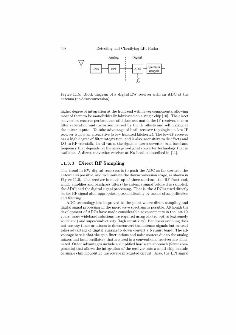
7/17/2019 1596932341 Intercept Radar.pdf
http://slidepdf.com/reader/full/1596932341-intercept-radarpdf 429/891
398 Detecting and Classifying LPI Radar
Figure 11.5: Block diagram of a digital EW receiver with an ADC at theantenna (no downconversion).
higher degree of integration at the front end with fewer components, allowing
most of them to be monolithically fabricated on a single chip [10]. The directconversion receiver performance still does not match the IF receiver, due tofilter saturation and distortion caused by the dc off sets and self mixing atthe mixer inputs. To take advantage of both receiver topologies, a low-IFreceiver is now an alternative (a few hundred kilohertz). The low-IF receiverhas a high degree of filter integration, and is also insensitive to dc off sets andLO-to-RF crosstalk. In all cases, the signal is downconverted to a basebandfrequency that depends on the analog-to-digital converter technology that isavailable. A direct conversion receiver at Ka-band is described in [11].
11.3.3 Direct RF Sampling
The trend in EW digital receivers is to push the ADC as far towards the
antenna as possible, and to eliminate the downconversion stage, as shown inFigure 11.5. The receiver is made up of three sections: the RF front end,which amplifies and bandpass filters the antenna signal before it is sampled;the ADC; and the digital signal processing. That is, the ADC is used directlyon the RF signal after appropriate preconditioning by means of amplificationand filtering.
ADC technology has improved to the point where direct sampling anddigital signal processing in the microwave spectrum is possible. Although thedevelopment of ADCs have made considerable advancements in the last 10years, more wideband solutions are required using electro-optics (extremelywideband) and superconductivity (high sensitivity). Bandpass sampling doesnot use any tuner or mixers to downconvert the antenna signals but insteadtakes advantage of digital aliasing to down convert a Nyquist band. The ad-
vantage here is that the gain fluctuations and noise sources due to the analogmixers and local oscillators that are used in a conventional receiver are elimi-nated. Other advantages include a simplified hardware approach (fewer com-ponents) that allows the integration of the receiver onto a multi-chip moduleor single chip monolithic microwave integrated circuit. Also, the LPI signal

7/17/2019 1596932341 Intercept Radar.pdf
http://slidepdf.com/reader/full/1596932341-intercept-radarpdf 430/891
Strategies for Intercepting LPI Radar Signals 399
Figure 11.6: Block diagram of a reconfigurable direct RF sampling architec-ture [13].
information is captured prior to significant analog distortion and mixer non-linearities. Direct RF sampling also allows the receiver to be reconfigurableto support software-defined detection and classification algorithms.
If a single fixed clock is used (partially reconfigurable), multiple bands canbe covered as long as the bands alias to the same intermediate frequency band.Direct sampling works well for low RF signals but places severe constraintson the ADC for higher analog input frequencies due to the eff ect of clock
jitter or clock uncertainty [12]. To achieve arbitrary tuning over a wide RFrange, however, the RF sample clock must be tunable or selectable becauseof the problems with signal recovery on the boundaries of the Nyquist bandsgenerated by a fixed RF sample clock [13].
A reconfigurable direct RF sampling architecture that off ers flexible tun-ing to cover high RF bands is shown in Figure 11.6. The RF input from theLNA is filtered by the antialiasing filter H (ω) for the band of interest. Thefilter output signal is then sampled by pulses2 at a rate of f S 1 and filteredby a continuous time interpolation filter which also serves as an antialiasingfilter for the ADC that is sampling at a rate of f S 2. Sampling is achievedin two stages. In the first stage, the RF signal is bandpass filtered and sam-pled using an impulse sampling device without quantization. After tunablepulse sampling, the signal is continuous time lowpass or bandpass filtered togenerate an IF signal that is then sampled by a conventional ADC.
By using continuous time filtering after the first stage sampling, the ADCsample clock may be completely decoupled from the RF sample clock to al-
low arbitrary tuning without impacting the ADC sample rate. That is, byseparating the sampling and quantization processes into multiple stages, the
2Pulse sampling is a technique that can be used for direct RF sampling at much higherfrequencies than track and hold based sampling. The basic requirements for high RF pulsesampling are narrow pulse width and low pulse amplitude jitter, in addition to the lowtime jitter required in any direct RF sampling scheme [13].

7/17/2019 1596932341 Intercept Radar.pdf
http://slidepdf.com/reader/full/1596932341-intercept-radarpdf 431/891
400 Detecting and Classifying LPI Radar
jitter and clock speed requirements on the ADC can be relaxed. A high de-gree of reconfigurability in tuning range and bandwidth is achieved by usinga tunable (or selectable) antialiasing filter before the first stage of samplingand by using a tunable sample clock in the first stage of sampling. Extensionof this receiver architecture to an analog-to-information receiver is describedin [14]. Motivated by recent developments in compressed sensing the receiverperforms frequency modulated pulsed sampling at sub-Nyquist rates to com-press a broadband RF environment into an analog interpolation filter andsamples the signal at the information rate rather than using the Shannonbandwidth criteria. The receiver uses structured nonuniform sampling to im-plement a direct analog-to-information receiver that is eff ective at recoveringsignals that have a sparse frequency domain representation [14].
11.4 Demodulation of the LPI Waveform
LPI signals attempt to make the detection and demodulation process impos-sible. The EW intercept receiver requires a large processing gain to detect theLPI emission, and extract the parameters of the signal. This is followed bythe task of classification. Classification requires sorting the signal into groupshaving similar parameters (clustering). Parameters such as carrier frequency,bandwidth, modulation period, modulation bandwidth, and time of arrivalare a few of the parameters that distinguish one signal from another. Cor-relation with existing signals in a database (identification) can then aid insignal tracking and response management.
To identify the emitter parameters, Fourier analysis techniques using the
FFT have been used as the basic tool. From this basic tool, more com-plex signal processing techniques have evolved, such as the short-time Fouriertransform, in order to track the signal parameters over time. More sophisti-cated techniques have also been developed, called time-frequency and bifre-quency distributions in order to identify the exotic modulation schemes usedby the LPI radar [15]. These techniques include the Wigner distribution,Choi-Williams distribution, quadrature mirror filtering, and cyclostationaryprocessing. The use of these techniques to extract the parameters from someof the well-known LPI modulations is the subject of the remaining chapters.
11.5 EW Receiver Challenges
The steady increase in sophistication of radar systems has resulted in an elec-tromagnetic environment where very few pulses can now be expected. Inaddition, pulse-to-pulse PRI agility and frequency agility now make it ex-tremely difficult to identify a specific emitter, especially when only a fewpulses are intercepted (e.g., from a track-while-scan or LPI radar). LPI CW

7/17/2019 1596932341 Intercept Radar.pdf
http://slidepdf.com/reader/full/1596932341-intercept-radarpdf 432/891
Strategies for Intercepting LPI Radar Signals 401
radar, as well as digital-pulsed radar, now transmit with an enormous numberof new, complex modulations. These complex modulations can result in manyreports for a single diverse emitter, making correct signal identification dif-ficult. Furthermore, these modern radars will essentially blind existing EWdesigns, resulting in a situation where the warning receivers can no longerhandle even those radars they were designed to intercept. For example, anexisting EW might be subject to performance degradation, due to possibleinterference from modern pulse-Doppler radars transmitting from friendlyplatforms.
Other problem situations include the fact that many communication CWsignals are now within the radar spectrum. A significant problem can alsooccur when the intercept receiver processes signals with parameters outsideits bounds. This can often cause resets that bring the system off -line forseveral minutes. Resets can also occur when the receiver processes signalsthat are near the internal thresholds. Finally, a significant problem for thereceiver is a failure to intercept a threat emitter that is present (including itsmodulation parameters). This is more likely to happen with LPI emitters.Today’s modern EW receivers must have the ability to intercept both pulseradar signals and CW signals within a wide bandwidth (e.g., 0.5—100 GHz).The trend is to share a common aperture, and combine the communications,the EW, and radar functions requiring less antenna apertures.
Another serious problem for the EW receiver is the presence of ultra-wideband sources such as spread spectrum communication signals, impulse
jammers, and impulse radar. The impact of ultrawideband synthetic apertureradar (SAR), and inverse SAR (or ISAR) imaging radar, and high range
resolution profi
ling sensors, must also be considered. These sources (whetherintercepted intentionally or not) can significantly raise the noise floor of thereceiver, disabling the ability of the EW receiver to see the important threatsof interest. Consequently, the ability to reject unwanted signals is now just asimportant as the ability to process the signals of interest. Wideband receiversrequire adaptive notch (band reject) filters at the front end, to exclude theseunwanted signals. YIG (yttruim iron garnet) filters are often used. Adaptivethresholds can also be used to increase sensitivity. The EW receiver mustalso have high power detection and protection circuits at the front end, toprotect itself from deliberate destruction by microwave weapons and otherdirected energy weapons. One high-power microwave pulse at the front endof the intercept receiver can destroy the EW receiver function, causing totalfailure of the ES/ELINT system onboard the aircraft.
The EW receiver and associated EA must also be able to provide the quickreaction mode necessary to counter the new modern range-Doppler imagingmissiles. These missiles will use FMCW modes such as SAR, ISAR and highrange-Doppler imaging in order to improve target aimpoint accuracy, and toreject decoys that are launched. As we discussed in Chapter 1 and demon-strated in Chapter 9, power-managed seekers adjust the transmitter power

7/17/2019 1596932341 Intercept Radar.pdf
http://slidepdf.com/reader/full/1596932341-intercept-radarpdf 433/891
402 Detecting and Classifying LPI Radar
such that the received power at the EW receiver is kept constant (or is de-creasing). EW receivers that prioritize incoming threats based on a change of the received signal amplitude will be vulnerable to the power-managed LPIseekers. These power-managed emitters must also be detected and processedcorrectly. Advanced missiles will also use dual mode seekers (e.g., an antira-diation missile seeker combined with an active millimeter wave LPI seeker)that must also be identified and countered.
Finally, the EW receiver must be able to disseminate all onboard detec-tions in real time sometimes referred to as real time out of the cockpit (RTOC).RTOC data is critical in a network-centric architecture in order to providemultiplatform targeting and geolocation. Also the ability to accept real time
data in the cockpit (RTIC), and utilize the off board (multispectral) sensordata, is an important capability in order for the platform to precisely targetits weapons or electronic attack. In this way the intercept receiver can bea major player in a multiplatform time diff erence of arrival (TDOA)-basedgeolocation network with, for example, Rivet Joint. The data fusion alsoexploits any off board and multispectral signals intelligence (SIGINT) datareceived.
Specific emitter identification (SEI) attempts to fingerprint the emittersthat are intercepted. SEI can also be used for improved tracking and dein-terleaving. A number of algorithms have been investigated for doing SEI,but their details remain classified. More importantly, however, is the factthat future SEI systems must be standardized for interoperability betweenplatforms and organizations (especially since the dividing line between RWRand ELINT is fast going away). That is, the success in SEI will ultimately
lie in the infrastructure (dissemination of databases, correlation of absolutes,organized collection of targets), and not so much in the algorithms that areused.
11.6 Concluding Remarks
The trend in intercept receivers is toward digital receivers and the conceptof digital antennas (ADC at the antenna). The future digital receiver willincorporate optical technologies for speed and bandwidth, and will also in-corporate high-temperature superconductors for sensitivity. Networking theEW receiver within an information, sensor, and shooter grid will allow thesharing of intercept data. The use of swarm architectures will also becomemore prevalent. In the following chapters we assume that the signal is digi-tized in the receiver, and we mainly focus on the signal processing methodsused to extract the LPI waveform parameters to classify the signals.
7/17/2019 1596932341 Intercept Radar.pdf
http://slidepdf.com/reader/full/1596932341-intercept-radarpdf 434/891
Strategies for Intercepting LPI Radar Signals 403
References[1] Schrick, G., and Wiley, R. G., “Interception of LPI radar signals,” IEEE
International Radar Conference , pp. 108—111, 1990.
[2] Wiley, R. G., Electronic Intelligence: The Interception of Radar Signals,Artech House Publishers, Dedham, MA, 1985.
[3] Lee, J. P. Y., “Interception of LPI radar signals,” Defence Research Estab-lishment Ottawa, Technical Note 91-23, Nov. 1991.
[4] Bonabeau, E., Dorigo, M., and Theraulaz, G., Swarm Intelligence From Nat-ural to Arti fi cial Systems, Oxford University Press, New York, 1999.
[5] Tsui, J. B. Y., and Stephens, J. P. Sr., “Digital microwave receiver technol-ogy,” IEEE Trans. on Microwave Theory and Techniques Vol. 50, No. 3, pp.
699—705, March 2002.[6] Rodrigue, S. M., Bash, J. L., and Haenni, M. G., “Next generation broadband
digital receiver technology,” The 15th Annual AESS/IEEE Symposium , pp.13—20, 14—15 May 2002.
[7] Gross, F. B., and Chen, K., “Comparison of detectability of traditional pulsedand spread spectrum radar waveforms in classic passive receivers,” IEEE Trans. on Aerospace and Electronic Systems, Vol. 41, No. 2, pp. 746—751,April 2005.
[8] Gross, F. B., and Connor, J., “Comparison of detectability of radar compres-sion waveforms in classic passive receivers,” IEEE Trans. on Aerospace and Electronic Systems, Voltt . 43, No. 2, pp. 789—795, April, 2007.
[9] Shieh, C-S, and Lin, C-T., “A vector neural network for emitter identifi-cation,” IEEE Trans. on Antennas and Propagation, Vol. 50, No. 8, pp.
1120—1127, Aug. 2002.
[10] Pekau, H., and Haslett, J. W., “A comparison of analog front end architec-tures for digital receivers,” Proc. of the IEEE CCECE/CCGEI , Saskatoon,May 2005.
[11] Tatu, S. O., et al., “Ka-band direct digital receiver,” IEEE Trans. on Mi-crowave Theory and Techniques , Vol. 50, No. 11, pp. 2436—2442, Nov. 2002.
[12] Chalvatzis, T., Gagnon, E., and Wight, J. S., “On the eff ect of clock jitterin IF and RF direct sampling systems,” 3rd International IEEE NEWCAS Conference , pp. 63—66, 19—22 June 2005.
[13] Fudge, G. L., Chivers, M. A., Ravindran, S., Bland, R. E., and Pace, P.E., “A reconfigurable direct RF receiver architecture,” Proc. of the IEEE International Symposium on Circuits and Systems , May 2008.
[14] Fudge, G. L., Bland, R. E., Chivers, M. A., Ravindran, S., Haupt, J. andPace, P. E., “A Nyquist folding analog-to-information receiver,” Proc. of the Asilomar Conf. on Signals, Computers and Signal Processing , Nov. 2008.
[15] Stephens, J. P., “Advances in signal processing for electronic warfare,” IEEE Aerospace and Electronic Systems Magazine , pp. 31—38, Nov. 1996.

7/17/2019 1596932341 Intercept Radar.pdf
http://slidepdf.com/reader/full/1596932341-intercept-radarpdf 435/891
7/17/2019 1596932341 Intercept Radar.pdf
http://slidepdf.com/reader/full/1596932341-intercept-radarpdf 436/891
Chapter 12
Wigner-Ville Distribution
Analysis of LPI RadarWaveforms
In Chapter 11, it was shown that tomorrow’s digital intercept receiver mustincorporate a time-frequency analysis capability in order to identify the LPImodulation types and also extract the LPI signal’s parametric data. TheWigner-Ville Distribution (WVD), introduced by Wigner in 1932 as a phaserepresentation in quantum statistical mechanics [1] and separately by Villein 1948 addressing the question of a joint distribution function [2], simul-
taneously gives the representation of a signal in both time and frequencyvariables. The WVD has been noted as one of the more useful bilinear time-frequency analysis techniques for signal processing. In this chapter, the WVDis presented and used to analyze the signals discussed in Part I. Extractionof the signal parameters is also emphasized. The main objective is that bystudying the results and correlating the signal parameters that are revealed,the user can learn to determine the presence of a particular LPI signal andto recognize the LPI modulation characteristics under various signal-to-noiseratios. We also show how well we can distinguish among several waveformsthat have similar time and frequency characteristics. Multiple signal analysisis left as an exercise for the reader. By using the Wigner analysis tools, anintercept receiver can come close to having a processing gain near the LPIradar’s matched filter processing gain. The WIGNER folder on the CD pro-
vides the MATLAB tools that can be used to re-create any of the figurespresented, as well as generate new and useful results.
405
7/17/2019 1596932341 Intercept Radar.pdf
http://slidepdf.com/reader/full/1596932341-intercept-radarpdf 437/891
406 Detecting and Classifying LPI Radar
12.1 Wigner-Ville DistributionThe WVD has been used in many fields of engineering. These include opticalimplementations of the WVD [3], medical applications [4—6], image analysis[7, 8], target detection [9, 10], and the analysis of nonstationary (LPI) signals[11—14].
The WVD exhibits the highest signal energy concentration in the time-frequency plane for linearly modulated signals, but has drawbacks in thecase of nonlinear frequency modulated signals. To improve the concentrationwhere nonlinear modulations are present, various higher-order time frequencyrepresentations have been investigated [15]. The WVD also contains inter-fering cross terms (or ghost terms) between every pair of signal components.As illustrated in the examples that follow, the presence of the cross terms
sometimes make it difficult to determine the LPI modulation parameters.A good review of bilinear transforms and their use in signal analysis is
given in [16]. The influence that the cross term interference has on the WVDis analyzed in [17, 18]. The extension of the WVD to discrete time signalshas been discussed in [19, 20] and a formulation to remove the cross termshas been reported in [21, 22]. Below, we begin with the definition of theWVD, and then present a windowed version of the WVD, the pseudo WVD(PWVD) which is useful in the signal processing of the digital signals withinthe receiver.
12.1.1 Continuous WVD
The WVD of a continuous one-dimensional function (or input signal) x(t) is
given by [23]
W x(t,ω) =
∞
−∞
x
t + τ
2
x∗
t− τ
2
e−jωτ dτ (12.1)
where t is the time variable, ω is the angular frequency variable (2πf ), and the∗ indicates a complex conjugate. The WVD is a three-dimensional functiondescribing the amplitude of the signal as a function of time and frequency.Since the LPI emitter modulations vary the compression of the CW waveformas a function of time, these types of time-frequency distributions give a higherprobability of detecting the modulation parameters. The WVD can also bedefined from the Fourier transform X (ω) of x(t) by
W X(ω, t) = 12π
∞−∞
X ω + ω0
2
X ∗
ω − ω0
2
e−jω0tdω0 (12.2)
From (12.1) and (12.2), the following relation is obtained:
W x(t,ω) = W X(ω, t) (12.3)

7/17/2019 1596932341 Intercept Radar.pdf
http://slidepdf.com/reader/full/1596932341-intercept-radarpdf 438/891
Wigner-Ville Distribution Analysis of LPI Radar Waveforms 407
That is, the WVD of the spectra of a signal can be determined simply fromthat of the time functions by an interchange of the frequency and time vari-ables. This shows the symmetry between space and frequency domain defin-itions [23].
Equation (12.1) implies that evaluation of the WVD is a noncausal oper-ation. As such, this expression does not lend itself to real-time evaluation.This limitation is overcome by first applying the WVD analysis to a sampledtime series x(), where is a discrete time index from −∞ to ∞. The discreteWVD is defined as
W (, ω) = 2∞
n=−∞
x( + n)x∗(− n)e−j2ωn (12.4)
Windowing the data results in the pseudo-WVD and is defined by [17]
W (,ω) = 2N −1
n=−N +1
x( + n)x∗(− n)w(n)w(−n)e−j2ωn (12.5)
where w(n) is a length 2N − 1 real window function with w(0) = 1. Usingf (n) to represent the kernel function
f (n) = x( + n)x∗(− n)w(n)w(−n) (12.6)
the PWVD becomes
W (, ω) = 2N −1
n=−N +1
f (n)e−j2ωn (12.7)
The choice of N (usually a power of 2) greatly aff ects the computationalcost, as well as the time-frequency resolution, of the PWVD output. A largeN gives a higher time-frequency resolution since it influences the frequencyresolution in (12.7). When the continuous variable ω in (12.7) is sampledto produce a suitable form of the discrete Fourier transform (DFT), a largerN also gives more output samples, yielding a smoother result [24]. Themaximum value of N is limited by
N ≤ M + 1
2 (12.8)
where M is the data length.
Once N is chosen, the kernel function can be generated. Since
f (n) = f ∗ (−n) (12.9)
only f (n) needs to be computed for n ≥ 0. A block diagram of the PWVDkernel generation for N = 8 is shown in Figure 12.1, where v(n) = w(n)w(−n).

7/17/2019 1596932341 Intercept Radar.pdf
http://slidepdf.com/reader/full/1596932341-intercept-radarpdf 439/891
408 Detecting and Classifying LPI Radar
Figure 12.1: The computational structure for an N = 8 PWVD kernel gen-eration [24] ( c1989 IEEE).
Here the input signal enters the buff er register from the left and shifts to theright after each kernel generation. The right-most element is disposed afterthe next shift.
The PWVD can detect the presence of LPI signals, as well as extract thesignal’s modulation characteristics. For an intercept receiver, it is importantthat the computation be done in real time or near real time. From thePWVD expression in (12.7), we notice that it is computationally expensive todirectly compute the PWVD. Boashash et al. [25] have presented an efficientalgorithm to compute the discrete PWVD. The algorithm is presented below.
To begin, the continuous frequency variable ω is sampled as
ω = πk
2N (12.10)
where k = 0, 1, 2, · · · , 2N − 1 (2N samples). The kernel indexes are modifiedto fit the standard DFT:
W , π
k2N
= 2
N −1n=−N +1
f (n)exp− j2
πnk
2N
(12.11)
or
W
, πk
2N
= 2
2N −1n=0
f (n)exp
−
j2πnk
2N
(12.12)

7/17/2019 1596932341 Intercept Radar.pdf
http://slidepdf.com/reader/full/1596932341-intercept-radarpdf 440/891
Wigner-Ville Distribution Analysis of LPI Radar Waveforms 409
where
f (n) =
⎧⎨⎩
f (n), 0 ≤ n ≤ N − 10, n = N f (n− 2N ), N + 1 ≤ n ≤ 2N − 1
(12.13)
Since the kernel is a symmetric function, the DFT of the kernel is always real.The resulting PWVD using 2N samples is
W (, k) = 22N −1n=0
f (n)exp
−
jπkn
N
(12.14)
Equation (12.14) is the algorithm implemented, and several examples areshown in the next section to illustrate the properties of the computation.
12.1.2 Example Calculation: Real Input Signal
Consider an example using a real input signal
x() = 2, 4, 3, 6, 1, 7 (12.15)
where N = 3 and the length of the input signal x() is 2N = 6. Here = −3,−2,−1, 0, 1, 2 and is the discrete time index in the range −N toN − 1. Note that x = 0 for ≤ −4 or ≥ 3. From (12.13), with N = 3,
f (n) =
⎧⎨
⎩
f (n), 0 ≤ n ≤ 20, n = 3f (n− 6), 4 ≤ n ≤ 5
(12.16)
From (12.6) f −3(n) ( = −3), for input signal x() is computed as follows:
f −3(n = 0) = x(−3) · x∗(−3) = 2 · 2 = 4
f −3(n = 1) = x(−2) · x∗(−4) = 4 · 0 = 0
f −3(n = 2) = x(−1) · x∗(−5) = 3 · 0 = 0
f −3(n = 3) = 0
f −3(n = 4) = x(1) · x∗(−7) = 1 · 0 = 0
f −3(n = 5) = x(2) · x∗(−8) = 7 · 0 = 0
So, from 12.13, f −3 = 4, 0, 0, 0, 0, 0. Similarly for f 0, ( = 0),
f 0(n = 0) = x(0) · x∗(0) = 6 · 6 = 36
f
0(n = 1) = x(1) · x∗
(−1) = 1 · 3 = 3f 0(n = 2) = x(2) · x∗(−2) = 7 · 4 = 28
f 0(n = 3) = 0
f 0(n = 4) = x(−2) · x∗(2) = 4 · 7 = 28
f 0(n = 5) = x(−1) · x∗(1) = 3 · 1 = 3

7/17/2019 1596932341 Intercept Radar.pdf
http://slidepdf.com/reader/full/1596932341-intercept-radarpdf 441/891
410 Detecting and Classifying LPI Radar
Figure 12.2: The kernel f (n) matrix for the real six input example.
and so, f 0 = 36, 3, 28, 0, 28, 3. Repeating the above procedure, the kernelmatrix for all values = −4 to 3, and n = 0 to 5 is as shown in Figure 12.2.
The second step after the kernel transformation is to use (12.14) to calcu-late the Wigner distribution. As an example of the calculation, one can pickany and k to examine the values inside the PWVD matrix. For example,
choose = 1, k = 2, with N = 3. The PWVD is
W ( = 1, k = 2) = 22N −1n=0
f (n)exp
− j
πkn
N
= 22·3−1n=0
f (n)exp
− j
π2n
3
= 25
n=0
f (n)exp
− j
2πn
3
(12.17)
From the kernel matrix in Figure 12.2, the kernel function for = 1 is f 1(n) =1, 42, 0, 0, 0, 42. So from (12.17), the PWVD for = 1, k = 2 (6 terms) is
W (1, 2) = 2f 1(0) · exp
− j
2 · π · 0
3
+ 2f 1(1) · exp
− j
2 · π · 1
3
+ 2f 1(2) · exp
− j
2 · π · 2
3
+ 2f 1(3) · exp
− j
2 · π · 3
3

7/17/2019 1596932341 Intercept Radar.pdf
http://slidepdf.com/reader/full/1596932341-intercept-radarpdf 442/891
Wigner-Ville Distribution Analysis of LPI Radar Waveforms 411
Figure 12.3: The PWVD matrix W (, k) for the real six input example.
+ 2f 1(4) · exp
− j
2 · π · 4
3
+ 2f 1(5) · exp
− j
2 · π · 5
3
= 2 · 1 · (0) + 2 · 42 · (−0.5000− 0.8660i)
+ 2 · 0 + 2 · 0 + 2 · 0 + 2 · 42 · (0.5000 + 0.8660i)
W (1, 2) = −82
Repeating the above procedure gives the PWVD matrix at each discrete timeindex = −4 to 3 for each discrete frequency index k = 0 to 5. The resultis a symmetric matrix about k = 3, as shown in Figure 12.3. An importantfeature of the PWVD is that all the components in the matrix are real. Otherimportant properties of the PWVD are given in [3, 4, 7].
12.1.3 Example Calculation: Complex Input Signal
To demonstrate the PWVD computation for a complex input, consider thesignal
x = I + jQ (12.18)
where
I = cos(2πf ct) (12.19)
Q = sin(2πf ct) (12.20)
If the carrier frequency f c = 1 kHz, sampling frequency, f s = 7 kHz, andt ∈ 0, 1/f s, 2/f s, . . . , 7/f s, then the first eight input points for the discrete

7/17/2019 1596932341 Intercept Radar.pdf
http://slidepdf.com/reader/full/1596932341-intercept-radarpdf 443/891
412 Detecting and Classifying LPI Radar
Figure 12.4: The kernel matrix for the complex eight input example.
time index = −4 to 3 is
x() = 1 + 0i, 0.62 + 0.78i, −0.22 + 0.97i, −0.90 + 0.43i,
−0.90− 0.43i, −0.22− 0.97i, 0.62− 0.78i, 1 + 0i (12.21)
Consider the value when = 0, n = 3. Using (12.13) with an input length2N = 8 or N = 4. The kernel is
f
=
⎧⎨⎩
f (n), 0 ≤ n ≤ 30, n = 4f (n− 8), 5 ≤ n ≤ 7
(12.22)
orf (n) = f (1), f (2), f (3), 0, f (−3), f (−2), f (−1) (12.23)
Since f (n) = x( + n) · x∗( − n), the kernel at = 0, n = 3 is f 0(3) =x(3) · x∗(−3) = 1 · (0.6235 + 0.7818i)∗ = 0.6235 − 0.7818i. Repeating thesame procedures as discussed in the real input case, the kernel matrix forthe complex eight input example is shown in Figure 12.4. Referring toFigure 12.4, we can calculate the PWVD when = −1. The kernel is
f −1(n) = 1.00, −0.22 + 0.97i, −0.90− 0.43i, 0.62− 0.78i,
0, 0.62 + 0.78, −0.90 + 0.43i, −0.22− 0.97i (12.24)

7/17/2019 1596932341 Intercept Radar.pdf
http://slidepdf.com/reader/full/1596932341-intercept-radarpdf 444/891
Wigner-Ville Distribution Analysis of LPI Radar Waveforms 413
Figure 12.5: The PWVD matrix for the complex eight input example.
Consider the case when = −1, k = 4. From (12.14), the PWVD for N = 4is
W ( = −1, k = 4) = 22N −1
n=0
f (n)exp− j
πkn
N
= 22·4−1n=0
f −1(n)
π4n
4
= 27
n=0
f −1(n) exp(− jnπ) (12.25)
From (12.24) and (12.25)
W ( = −1, k = 4) = 27
n=0
f −1(n) · exp(− jnπ) = −3.2073
Again, the PWVD matrix of the complex eight input samples is real. Thecomplete PWVD matrix is a symmetric 2N × 2N matrix. Figure 12.5 showsthe PWVD matrix of the complex eight input samples. Note this importantfeature: the PWVD is always real whether the input signal is real or complex.
Figure 12.6(a) shows a 3D mesh plot of the PWVD for the complex sig-nal example with eight inputs. This plot shows the magnitude in both the

7/17/2019 1596932341 Intercept Radar.pdf
http://slidepdf.com/reader/full/1596932341-intercept-radarpdf 445/891
414 Detecting and Classifying LPI Radar
time domain and the frequency domain. Note that it directly correlates withFigure 12.5. The peak corresponds to the 1-kHz carrier frequency.Figure 12.6(b) shows the corresponding PWVD contour plot. The contourplot is a 2D time-frequency plot that is useful for characterizing the time-frequency behavior of the signal. The magnitude is represented by a diff erentgray scale, as shown in the legend bar.
To see the marginal details of the PWVD, Figure 12.7(a) shows a plot of the PWVD obtained by rotating the mesh plot in Figure 12.6(a) to show
just the time axis with the eight samples. The time resolution is 1/f s.Figure 12.7(b) shows the marginal details in the frequency domain, and isobtained in the same manner as Figure 12.7(a). The carrier frequency is rep-resented by the peak in this plot, and shows up at 900 Hz, very close to thereal value 1 kHz. The frequency resolution f s/2/# samples is also indicated.
In summary both the real signal example and the complex signal exam-ple illustrate the mechanics of the PWVD calculation. The PWVD time-frequency results, when presented in the four diff erent plots, give a varietyof aspects so that the LPI signal and its modulation characteristics can bedetermined.
12.1.4 Two-Tone Input Signal Results
Now we consider the PWVD for a two-tone input (two carrier frequencies)with f c1 = 1 kHz and f c2 = 2 kHz. Now I = cos(2πf c1t) + cos(2πf c2t) andQ = sin(2πf c1t) + sin(2πf c2t).
Figure 12.8(a) shows the PWVD results for the two-tone signal in a 3Dtime-frequency mesh plot. In this plot the cross terms are stronger than thesignal terms, and show up with many peaks. Figure 12.8(b) is the 2D PWVDtime-frequency contour plot and shows the time dependence of the real signaland the cross terms.
Figure 12.9(a) shows the marginal time domain plot obtained by rotatingthe 3D mesh plot in Figure 12.8(a), to show only the time axis. This revealsthe cross terms as a series of positive and negative magnitude components inthe time domain. Figure 12.9(b) shows the frequency domain plot obtainedin the same manner, and reveals the two-carrier frequencies and the crossterm. Note that the shape and magnitude of the cross term is not like thetwo-carrier frequency components, and can be easily identified.
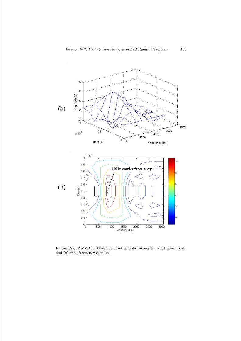
7/17/2019 1596932341 Intercept Radar.pdf
http://slidepdf.com/reader/full/1596932341-intercept-radarpdf 446/891
Wigner-Ville Distribution Analysis of LPI Radar Waveforms 415
Figure 12.6: PWVD for the eight input complex example: (a) 3D mesh plot,and (b) time-frequency domain.

7/17/2019 1596932341 Intercept Radar.pdf
http://slidepdf.com/reader/full/1596932341-intercept-radarpdf 447/891
416 Detecting and Classifying LPI Radar
Figure 12.7: PWVD for the eight input complex example: (a) 2D mesh intime domain, and (b) 2D mesh in frequency domain.
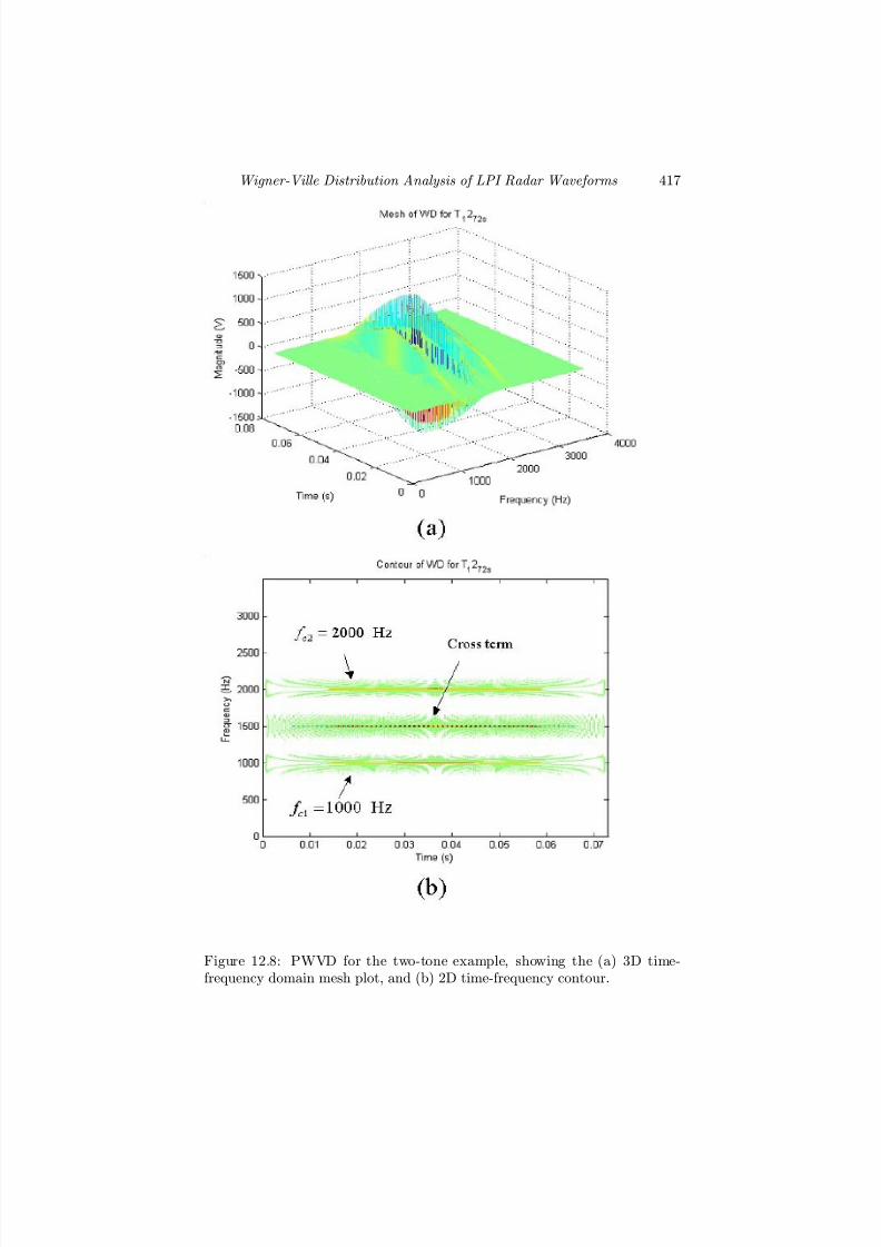
7/17/2019 1596932341 Intercept Radar.pdf
http://slidepdf.com/reader/full/1596932341-intercept-radarpdf 448/891
Wigner-Ville Distribution Analysis of LPI Radar Waveforms 417
Figure 12.8: PWVD for the two-tone example, showing the (a) 3D time-frequency domain mesh plot, and (b) 2D time-frequency contour.
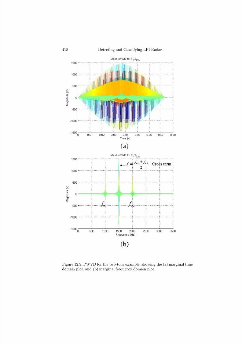
7/17/2019 1596932341 Intercept Radar.pdf
http://slidepdf.com/reader/full/1596932341-intercept-radarpdf 449/891
418 Detecting and Classifying LPI Radar
Figure 12.9: PWVD for the two-tone example, showing the (a) marginal timedomain plot, and (b) marginal frequency domain plot.

7/17/2019 1596932341 Intercept Radar.pdf
http://slidepdf.com/reader/full/1596932341-intercept-radarpdf 450/891
Wigner-Ville Distribution Analysis of LPI Radar Waveforms 419
Figure 12.10: Diagram of a triangular FMCW waveform.
12.2 FMCW Analysis
In this section, extraction of the signal parameters for two FMCW waveformexamples (see Chapter 4) are investigated. When measuring the parametersof the LPI modulations, in all cases the absolute value of the relative errorshould be reported. That is, if a∗ is a measurement value of a quantity whoseexact value is a, then the absolute value of the relative error r is defined by
r = a∗ − a
a =
Error
True value (12.26)
The time-frequency diagram of a triangular waveform is shown inFigure 12.10. For the examples, both signals are sampled by the ADC ata rate of f s = 7,000 Hz. The first signal examined is an FMCW wave-form with a center frequency of f c = 1,000 Hz, a modulation bandwidth of ∆F = 250 Hz, and a modulation period of tm = 20 ms. Figure 12.11(a)shows the PWVD frequency plot of the FMCW waveform. This graph canalso be compared with the PSD of the waveform (see Chapter 4). Note thepresence of the additional structure due to the triangular modulation. Thecarrier frequency can easily be identified and measured. The bandwidth of the signal can also be estimated. Figure 12.11(b) shows the time-frequencydistribution. Although cross terms are present in the output image, the
modulation bandwidth and the modulation period can be accurately iden-tified, as well as the carrier frequency. Figure 12.12(a) shows the PWVDimage for SNR = 0 dB and Figure 12.12(b) shows the PWVD image forSNR = −6 dB. The SNR is defined over f s/2. It is interesting to note thatthe carrier frequency, the modulation period, and the modulation bandwidthcan all be extracted, even with this amount of interference present in the

7/17/2019 1596932341 Intercept Radar.pdf
http://slidepdf.com/reader/full/1596932341-intercept-radarpdf 451/891
420 Detecting and Classifying LPI Radar
Figure 12.11: PWVD for an FMCW with ∆F = 250 Hz, tm = 20 ms (sig-nal only), showing the (a) marginal frequency domain plot, and (b) time-frequency plot.
7/17/2019 1596932341 Intercept Radar.pdf
http://slidepdf.com/reader/full/1596932341-intercept-radarpdf 452/891
Wigner-Ville Distribution Analysis of LPI Radar Waveforms 421
signal. Also note that this information is not available if only the PSD is cal-culated in the receiver. In summary, the PWVD technique works extremelywell for FMCW waveforms. The results for the ∆F = 500-Hz signal areshown in Appendix E.
12.3 BPSK Analysis
In this section we apply the PWVD and use it to investigate the propertiesof the BPSK signal discussed in Chapter 5. Parameters varied include thelength of the Barker code (N c = 7 or 11), the number of carrier cycles perBarker subcode (cpp), and the SNR (signal only, 0 dB, and −6 dB). We alsoinvestigate how many parameters of the signal can be extracted from the
PWVD results. All signals demonstrating the concepts have an f c = 1 kHzcarrier frequency, and a sampling frequency of f s = 7 kHz. Both frequencydomain and time domain plots are shown for the BPSK signals after thePWVD processing. The time-frequency domain results are the most useful.
The first signal, examined in Figure 12.13(a), has a carrier frequency of 1 kHz and can be clearly identified by the location of the highest or lowestpeak value. The carrier frequency can also be identified as the center of thesymmetric frequency distribution in Figure 12.13(b). Also, the relative peakmagnitude in Figure 12.13(a) is about 600, so the 3-dB bandwidth (or subcoderate) B, is the frequency range lying at 300 on both sides, which extends from500 Hz to 1,500 Hz. Since B = f c/cpp = 1,000 Hz, this correlates well. InFigure 12.13(a), if we look closely within the 3-dB bandwidth, one can findthat there are 15 peaks within the bandwidth. That is, there are 14 intervals
in the range from 500 Hz to 1,500 Hz. This number is always two times theBarker code length. In Figure 12.14, the 7-bit Barker code is examined withan SNR = 0 dB. Figure 12.14(a) shows the frequency domain where the 15intervals can be counted within the 3-dB bandwidth. Figure 12.14(b) showsthe corresponding time-frequency domain. In this particular case, not muchinformation is revealed.
Figure 12.15(a) shows the results for an 11-bit signal. In this case thereare 23 peaks within the 3-dB bandwidth (Barker code length N c = 11).Figure 12.15(b) shows the time-frequency results centered about the carrierfrequency of f c = 1,000 Hz.

7/17/2019 1596932341 Intercept Radar.pdf
http://slidepdf.com/reader/full/1596932341-intercept-radarpdf 453/891
422 Detecting and Classifying LPI Radar
Figure 12.12: PWVD for an FMCW with ∆F = 250 Hz, tm = 20-ms time-frequency plot for (a) SNR = 0 dB and (b) SNR = −6 dB.
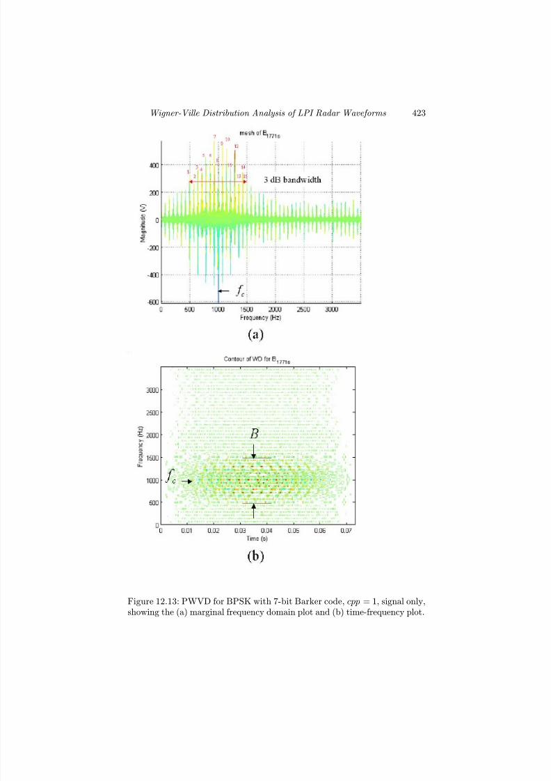
7/17/2019 1596932341 Intercept Radar.pdf
http://slidepdf.com/reader/full/1596932341-intercept-radarpdf 454/891
Wigner-Ville Distribution Analysis of LPI Radar Waveforms 423
Figure 12.13: PWVD for BPSK with 7-bit Barker code, cpp = 1, signal only,showing the (a) marginal frequency domain plot and (b) time-frequency plot.

7/17/2019 1596932341 Intercept Radar.pdf
http://slidepdf.com/reader/full/1596932341-intercept-radarpdf 455/891
424 Detecting and Classifying LPI Radar
Figure 12.14: PWVD for BPSK with 7-bit Barker code, cpp = 1, SNR =0 dB, showing the (a) marginal frequency domain plot and (b) time-frequencyplot.
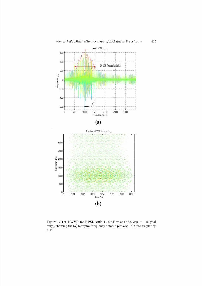
7/17/2019 1596932341 Intercept Radar.pdf
http://slidepdf.com/reader/full/1596932341-intercept-radarpdf 456/891
Wigner-Ville Distribution Analysis of LPI Radar Waveforms 425
Figure 12.15: PWVD for BPSK with 11-bit Barker code, cpp = 1 (signalonly), showing the (a) marginal frequency domain plot and (b) time-frequencyplot.
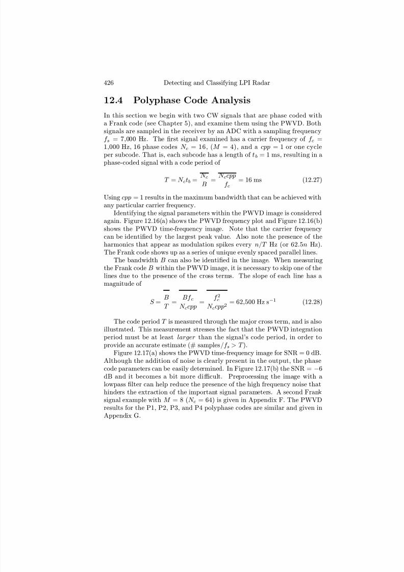
7/17/2019 1596932341 Intercept Radar.pdf
http://slidepdf.com/reader/full/1596932341-intercept-radarpdf 457/891
426 Detecting and Classifying LPI Radar
12.4 Polyphase Code AnalysisIn this section we begin with two CW signals that are phase coded witha Frank code (see Chapter 5), and examine them using the PWVD. Bothsignals are sampled in the receiver by an ADC with a sampling frequencyf s = 7,000 Hz. The first signal examined has a carrier frequency of f c =1,000 Hz, 16 phase codes N c = 16, (M = 4), and a cpp = 1 or one cycleper subcode. That is, each subcode has a length of tb = 1 ms, resulting in aphase-coded signal with a code period of
T = N ctb = N c
B =
N ccpp
f c= 16 ms (12.27)
Using cpp = 1 results in the maximum bandwidth that can be achieved withany particular carrier frequency.Identifying the signal parameters within the PWVD image is considered
again. Figure 12.16(a) shows the PWVD frequency plot and Figure 12.16(b)shows the PWVD time-frequency image. Note that the carrier frequencycan be identified by the largest peak value. Also note the presence of theharmonics that appear as modulation spikes every n/T Hz (or 62.5n Hz).The Frank code shows up as a series of unique evenly spaced parallel lines.
The bandwidth B can also be identified in the image. When measuringthe Frank code B within the PWVD image, it is necessary to skip one of thelines due to the presence of the cross terms. The slope of each line has amagnitude of
S = BT = Bf cN ccpp = f
2
cN ccpp2 = 62,500 Hz s−1 (12.28)
The code period T is measured through the major cross term, and is alsoillustrated. This measurement stresses the fact that the PWVD integrationperiod must be at least larger than the signal’s code period, in order toprovide an accurate estimate (# samples/f s > T ).
Figure 12.17(a) shows the PWVD time-frequency image for SNR = 0 dB.Although the addition of noise is clearly present in the output, the phasecode parameters can be easily determined. In Figure 12.17(b) the SNR = −6dB and it becomes a bit more difficult. Preprocessing the image with alowpass filter can help reduce the presence of the high frequency noise thathinders the extraction of the important signal parameters. A second Frank
signal example with M = 8 (N c = 64) is given in Appendix F. The PWVDresults for the P1, P2, P3, and P4 polyphase codes are similar and given inAppendix G.
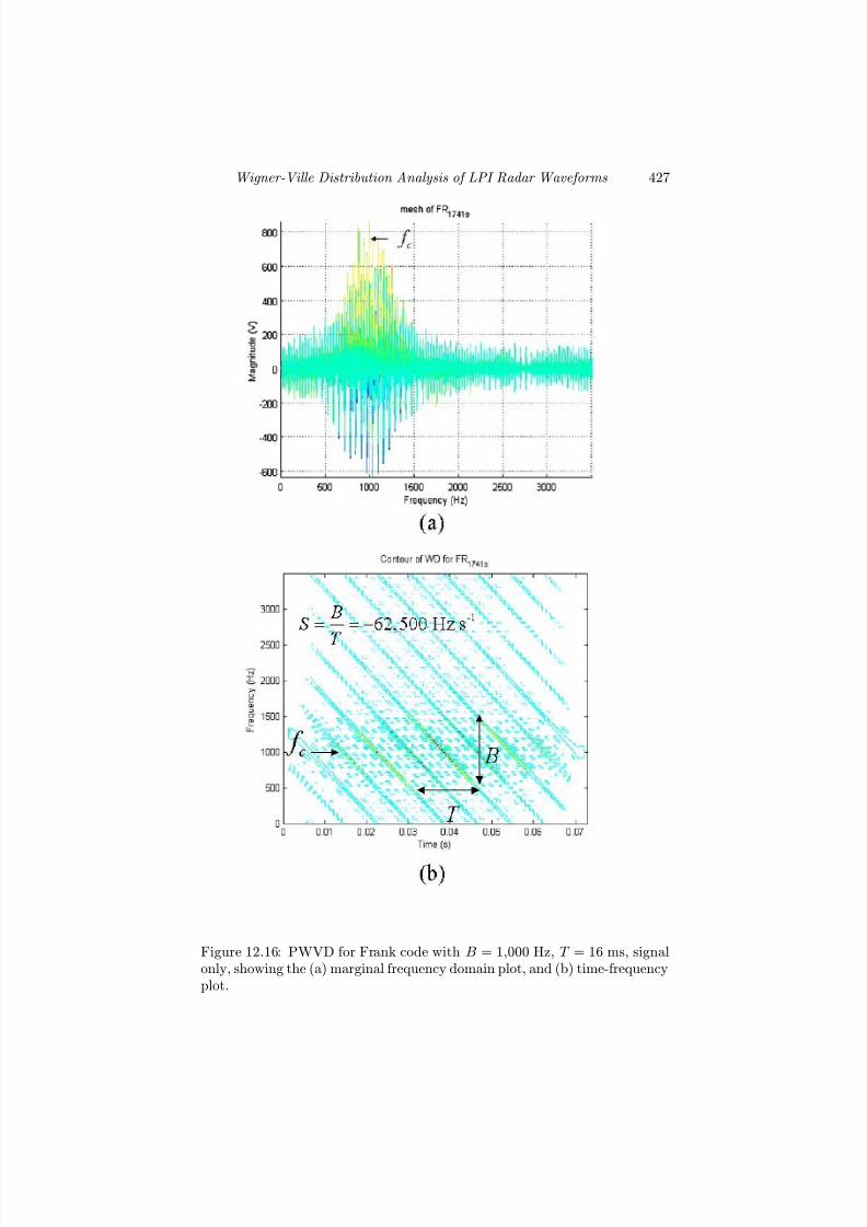
7/17/2019 1596932341 Intercept Radar.pdf
http://slidepdf.com/reader/full/1596932341-intercept-radarpdf 458/891
Wigner-Ville Distribution Analysis of LPI Radar Waveforms 427
Figure 12.16: PWVD for Frank code with B = 1,000 Hz, T = 16 ms, signalonly, showing the (a) marginal frequency domain plot, and (b) time-frequencyplot.

7/17/2019 1596932341 Intercept Radar.pdf
http://slidepdf.com/reader/full/1596932341-intercept-radarpdf 459/891
428 Detecting and Classifying LPI Radar
Figure 12.17: PWVD for Frank code with B = 1,000 Hz, T = 16 ms, time-frequency plot for (a) SNR = 0 dB, and (b) SNR = −6 dB.

7/17/2019 1596932341 Intercept Radar.pdf
http://slidepdf.com/reader/full/1596932341-intercept-radarpdf 460/891
Wigner-Ville Distribution Analysis of LPI Radar Waveforms 429
12.5 Polytime Code AnalysisIn this section an analysis of the polytime codes (see Chapter 5) using thePWVD is presented. The structure of the polytime codes (T1 through T4)within the PWVD are significantly diff erent, even though they were derivedfrom both step frequency and linear FM waveforms (as are the Frank codeand P1—P4).
The first signal examined is the T1 code with f c = 1,000 Hz and T = 16ms. The number of stepped frequency segments used is k = 4 (zero beatat the leading segment), and the number of phase states n = 2, T1(2).The sampling frequency of the ADC is f s = 7,000 Hz. Each segment is4 ms in duration, resulting in the overall code period of 16 ms. The fre-quency step between adjacent segments is 1/4 ms = 250 Hz with a total fre-
quency excursion of 1,000 Hz. Figure 12.18(a) shows the PWVD frequencydomain. Compared to the Frank and P1 through P4 codes, the T1(2) energyis more evenly distributed within the (approximately) same bandwidth. Alsonote that the harmonics are not uniformly spaced, due to the time modula-tion of the binary phase change. Figure 12.18(b) shows the time-frequencydistribution of the T1(2) code. The signal shows up as a set of vertical roof tops stacked next to each other, separated by T /2. Note that the carrier iseasily identified, as well as the measurement of the bandwidth B and codeperiod T (about the cross term).
To understand the bandwidth characteristics shown in Figure 12.18, thephase shift for the T1(2) is shown in Figure 12.19. Here the smallest phasechange shown is 4 samples long (0.571 ms). This results in a bandwidthexcursion of B = 1,750 Hz, which can be identified in Figure 12.18(b). Figure12.20(a) shows the signal for an SNR = 0 dB. The signal can still be identifiedas a T1(2) and the parameters can still be extracted. In Figure 12.20(b) withan SNR = −6 dB, no signal identification can be made and no parameterscan be extracted. The T2(2), T3(2), and T4(2) code examples are examinedin Appendix H.

7/17/2019 1596932341 Intercept Radar.pdf
http://slidepdf.com/reader/full/1596932341-intercept-radarpdf 461/891
430 Detecting and Classifying LPI Radar
Figure 12.18: PWVD for polytime code T1(2) with B = 1,750 Hz, T =16 ms, signal only showing the (a) marginal frequency domain plot, and(b) time-frequency plot.

7/17/2019 1596932341 Intercept Radar.pdf
http://slidepdf.com/reader/full/1596932341-intercept-radarpdf 462/891
Wigner-Ville Distribution Analysis of LPI Radar Waveforms 431
Figure 12.19: T1(2) phase shift showing a minimum subcode width of foursamples (0.571 ms), resulting in a bandwidth excursion of B = 1,750 Hz.
12.6 Distinguishing Between Phase Codes
The main objective of the previous sections was to examine the PWVD foreach of the important LPI phase modulations discussed in Part I. The inter-cept receiver running the PWVD must also be able to distinguish betweenthese phase modulations, in addition to extracting the signal parameters (asdescribed above).
To illustrate the similarities and diff erences, the phase modulations arecompared together in Figure 12.21. The Frank code, P1, P3, and P4 have thesame slope sign but, although similar, have diff erent time-frequency charac-teristics that can be used to identify the particular phase modulation. TheP2 has a diff erent slope. The distinguishing features, of course, depend onthe sampling period of the ADC, and any receiver nonlinearities that mightbe present.
The T1(2) (as well as T2—T4) are unique, since they contain time-frequencycomponents with both slope signs. Figures 12.22—12.25 show the PWVDtime-frequency results, and the corresponding phase states for the T1 throughT4, for comparison. Examination of these results shows that it is easy to dis-tinguish between the polytime codes, and also to distinguish them from the
Frank, P1, through P4, codes.

7/17/2019 1596932341 Intercept Radar.pdf
http://slidepdf.com/reader/full/1596932341-intercept-radarpdf 463/891
432 Detecting and Classifying LPI Radar
Figure 12.20: PWVD for T1(2) code with B = 1,750 Hz, T = 16 ms, time-frequency plot for (a) SNR = 0 dB, and (b) SNR = −6 dB.

7/17/2019 1596932341 Intercept Radar.pdf
http://slidepdf.com/reader/full/1596932341-intercept-radarpdf 464/891
Wigner-Ville Distribution Analysis of LPI Radar Waveforms 433
Figure 12.21: PWVD for (a) Frank code, (b) P1, (c) P2, (d) P3, and (e) P4codes.

7/17/2019 1596932341 Intercept Radar.pdf
http://slidepdf.com/reader/full/1596932341-intercept-radarpdf 465/891
434 Detecting and Classifying LPI Radar
Figure 12.22: PWVD for (a) T1(2) code, and (b) phase code showing mini-mum subcode with 18 samples (2.57 ms).

7/17/2019 1596932341 Intercept Radar.pdf
http://slidepdf.com/reader/full/1596932341-intercept-radarpdf 466/891
Wigner-Ville Distribution Analysis of LPI Radar Waveforms 435
Figure 12.23: PWVD for (a) T2(2) code, and (b) phase code showing mini-mum subcode with 36 samples (5.14 ms).

7/17/2019 1596932341 Intercept Radar.pdf
http://slidepdf.com/reader/full/1596932341-intercept-radarpdf 467/891
436 Detecting and Classifying LPI Radar
Figure 12.24: PWVD for (a) T3(2) code, and (b) phase code showing mini-mum subcode with six samples (0.86 ms).

7/17/2019 1596932341 Intercept Radar.pdf
http://slidepdf.com/reader/full/1596932341-intercept-radarpdf 468/891
Wigner-Ville Distribution Analysis of LPI Radar Waveforms 437
Figure 12.25: PWVD for (a) T4(2) code, and (b) phase code showing mini-mum subcode with seven samples (1 ms).

7/17/2019 1596932341 Intercept Radar.pdf
http://slidepdf.com/reader/full/1596932341-intercept-radarpdf 469/891
438 Detecting and Classifying LPI Radar
12.7 FSK and FSK/PSK AnalysisIn this section we examine the PWVD results for an FSK Costas signal anda hybrid PSK/FSK signal. The PWVD is used first to investigate the time-frequency characteristics of a Costas sequence 3, 2, 6, 4, 5, 1 kHz. Thesignal was generated with the costas.m program within the LPIT, using afrequency duration of t p = 0.005s and a sampling frequency of f s = 15,057Hz. This resulted in single frequency-hopping sequence consisting of 520 sam-ples. The PWVD marginal frequency domain is shown in Figure 12.26(a).Note that the frequencies in the sequence are clearly present, as well as thecross terms. The PWVD time-frequency image is shown in Figure 12.26. Thearrows indicate the positions of the Costas frequencies. Note that the timeaxis is reversed. That is, the frequency order begins at the right side of the
figure. The cross terms present tend to make the identification of the frequen-cies intricate, especially when the cross terms lie about one of the frequenciesin the code. In Figure 12.27(a, b), the time-frequency image is displayed forboth 0 dB and −6 dB, respectively. As expected, the identification becomesmore difficult.
With the FSK (Costas)/PSK signal, each frequency selected is phaseshifted with a 5-bit Barker code with cpp = 5 (five cycles per phase code).The results are shown in Figure 12.28(a, b) for the signal only, and SNR = 0dB, respectively. Note that although the cross terms are again significant, thefrequencies in the Costas code can be identified. For the FSK/PSK targetsignal described, the PWVD does not give good results, and no parameterscan be determined.
12.8 Summary
The PWVD theory was presented in this chapter and several examples wereused to demonstrate generating an efficient kernel function and the subsequentcalculation of the PWVD time-frequency results. Whether the signals are realor complex, the kernel and PWVD matrix are always real and symmetric.This is an important feature for the Wigner distribution and a good reasonwhy the PWVD can be used for accurate signal analysis (in spite of the crossterms present).
Apart from the parameters listed in the table, other signal characteristicscan be measured or estimated. For example, for the FMCW signal, knowing∆F and tm, the range resolution ∆R and the unambiguous range Ru may be
estimated. For the FSK Costas code, the identification of the signal is difficultdue to the ghost terms present. This is also the case for the FSK/PSK (binaryphase code) signal. For the FSK/PSK (target) signal reported, the PWVDwas not able to identify any meaningful signal parameters. This should notbe a surprise, considering the PACF, PAF results shown in Chapter 6.

7/17/2019 1596932341 Intercept Radar.pdf
http://slidepdf.com/reader/full/1596932341-intercept-radarpdf 470/891
Wigner-Ville Distribution Analysis of LPI Radar Waveforms 439
Figure 12.26: PWVD for Costas code sequence 3, 2, 6, 4, 5, 1 kHz, showingthe (a) marginal frequency domain, and (b) time-frequency image.

7/17/2019 1596932341 Intercept Radar.pdf
http://slidepdf.com/reader/full/1596932341-intercept-radarpdf 471/891
440 Detecting and Classifying LPI Radar
Figure 12.27: PWVD time-frequency image for Costas code sequence 3, 2,6, 4, 5, 1 kHz, showing (a) SNR = 0 dB, and (b) SNR = −6 dB.

7/17/2019 1596932341 Intercept Radar.pdf
http://slidepdf.com/reader/full/1596932341-intercept-radarpdf 472/891
Wigner-Ville Distribution Analysis of LPI Radar Waveforms 441
Figure 12.28: The PWVD for the FSK/PSK signal, showing the (a) signalonly, and (b) SNR = 0 dB.

7/17/2019 1596932341 Intercept Radar.pdf
http://slidepdf.com/reader/full/1596932341-intercept-radarpdf 473/891
442 Detecting and Classifying LPI Radar
The presentation of the PWVD results to a trained operator will allow thesignal parameters to be extracted, and can enable good classification resultsin moderate amounts of noise. A modern intercept receiver/analyzer wouldimplement a set of parallel processors; each designed to recognize, within aparticular frequency band, a particular class of waveforms that might occupythat band. The outputs would consist of pulse descriptor words containingestimates of the signal parameters. How well the PWVD processing performsthis task, as a function of its bandwidth (relative to the actual signal band-width) and the SNR in that bandwidth, is of primary concern and must beinvestigated. Autonomous classification and parameter extraction within anintercept receiver is a significantly harder problem, and is addressed furtherin Chapters 17 and 18.
References
[1] Wigner, E. P., “On the quantum correction for thermodynamic equilibrium,”Physics Review , Vol. 40, pp. 749—759, 1932.
[2] Ville, J., “Theorie et applications de la notion de signal analytique,” Cables
et Transmission , Vol 2A, pp. 61—74, 1948.
[3] Li, Y., Eichmann G., and Conner, M., “Optical Wigner distribution andambiguity function for complex signals and images,” Optics Communication ,Vol. 67, No. 3, pp. 177—179, July 1988.
[4] Clayton, R. H., and Murray, A., “Comparison of techniques for time-frequencyanalysis of the ECG during human ventricular fibrillation,” IEE Proc. on Sci-
ence and Measurement Technology, Vol. 145, No. 6, pp. 301—306, Nov. 1998.
[5] Darvish, N., and Kitney, R. I., “Time-frequency and time-scale methods in thedetection and classification of non-stationarities in human physiological data,”Record of the 28th Asilomar Conference on Signals, Systems and Computers ,Vol. 2, pp. 1085—1158, Oct. 31—Nov. 2, 1994.
[6] Millet-Roig, J., et al., “Time-frequency analysis of a single ECG: to discrimi-nate between ventricular tachycardia and ventricular fibrillation,” Computers
in Cardiology , pp. 711—714, 1999.
[7] Cristobal, G., Bescos J., and Santamaria, J., “Image analysis through theWigner distribution,” Applied Optics , Vol. 28, No. 2, pp. 262—271, Jan.1989.
[8] Gonzalo, C., et al., “Space-variant filtering through the Wigner distributionfunction,” Applied Optics , Vol. 28, No. 4, pp. 730—735, Feb. 1989.
[9] Haykin, S., and Bhattacharya, T., “Wigner-Ville distribution: an important
functional block for radar target detection in clutter,” Record of the 28th Asilomar Conference on Signals, Systems and Computers , Vol. 1, pp. 68—72,Oct. 31—Nov. 2, 1994.
[10] Kumar, P. K., and Prabhu, K. M. M., “Simulation studies of moving target-detection: a new approach with the Wigner-Ville distribution,” IEE Proc. on
Radar, Sonar and Navigation, Vol. 144, No. 5, pp. 259—265, Oct. 1997.

7/17/2019 1596932341 Intercept Radar.pdf
http://slidepdf.com/reader/full/1596932341-intercept-radarpdf 474/891
Wigner-Ville Distribution Analysis of LPI Radar Waveforms 443
[11] Milne, P.R., and Pace, P. E., “Wigner distribution detection and analysis of FMCW and P-4 polyphase LPI waveforms,” IEEE International Conference
on Acoustics, Speech, and Signal Processing, Vol. 4, pp. 3944—3947, 2002.
[12] Taboada, F., et al., “Intercept receiver signal processing techniques to de-tect low probability of intercept radar signals,” Proc.of the Fifth Nordic Sig-
nal Processing Symposium , Hurtigruta Tromso-Trondheim, Norway, 4—7 Oct.2002.
[13] Barbarossa, S., “Parameter estimation of undersampled signals by Wigner-Ville analysis,” IEEE International Conference on Acoustics, Speech, and
Signal Processing , ICASSP-91, Vol. 5, pp. 3253—3256, April 14-17, 1991.
[14] Gau, J-Y, “Analysis of low probability of intercept (LPI) radar signals usingthe Wigner Distribution,” Naval Postgraduate School Master’s Thesis, Sept.2002.
[15] Katkovnik, V., and Stankovic, L., “Instantaneous frequency estimation usingthe Wigner distribution with varying and data-driven window length,” IEEE
Trans. on Signal Processing , Vol. 46, No. 9, pp. 2315—2325, Sept. 1998.
[16] Chen, V. C., and Ling, H., Time-Frequency Transforms for Radar Imaging
and Signal Analysis , Artech House, Inc., Norwood, MA, 2002.
[17] Stankovic, L., and Stankovic, S., “On the Wigner distribution of discrete timenoisy signals with application to the study of quantization eff ects,” IEEE
Trans. on Signal Processing , Vol. 42, No. 7, pp. 1863—1867, July 1994.
[18] Stankovic, L., “Algorithm for the Wigner distribution of noisy signals reali-sation,” IEE Electronics Letters , Vol. 34, No. 7, pp. 622—623, April 1998.
[19] O’Neill, J. C., Flandrin, P., and Williams, W. J., “On the existence of discreteWigner distributions,” IEEE Signal Processing Letters , Vol. 6, No. 12, pp.
304—306, Dec. 1999.[20] Claasen, T. A. C. M., and Mecklenbrauker, W. F. G., “The Wigner
distribution—a tool for time-frequency signal analysis, Part II: Discrete-timesignals,” Phillips Journal of Research , Vol. 35, No. 4/5, pp. 276—300, 1980.
[21] Kadambe, S., and Adali, T., “Application of cross term deleted Wigner rep-resentation (CDWR) for sonar target detection/classification,” Record of the
32nd Asilomar Conference on Signals, Systems & Computers, Vol. 1, pp.822—826, Nov. 1—4, 1998.
[22] Kadambe, S., and Orr, R., “Comparative study of the cross term deletedWigner and cross biorthogonal representations,” Record of the 31st Asilomar
Conference on Signals, Systems & Computers, Vol. 2, pp. 1484—1488, Nov.2—5, 1997.
[23] Claasen, T. A. C. M., and Mecklenbrauker, W. F. G., “The Wigner
distribution— a tool for time-frequency signal analysis, Part I: Continuous-time signals,” Phillips Journal of Research , Vol. 35, No. 3, pp. 217—250,1980.
[24] Sun, M., et al., “A Wigner spectral analyzer for nonstationary signals,” IEEE
Trans. on Instrumentation and Measurement, Vol. 38, No. 5, pp. 961—966,Oct. 1989.

7/17/2019 1596932341 Intercept Radar.pdf
http://slidepdf.com/reader/full/1596932341-intercept-radarpdf 475/891
444 Detecting and Classifying LPI Radar
[25] Boashash, B. and Black, P. J., “An efficient real-time implementation of theWigner-Ville distribution,” IEEE Trans. on Acoustics, Speech and Signal
Processing , Vol. ASSP-35, No. 11, pp. 1611—1618, Nov. 1987.
Problems
1. (a) Using the LPIT, generate the default FMCW waveform and thedefault P4 waveform. Load both signals into MATLAB, and truncatesuch that they both have the same size (be sure to at least include oneto two code periods of each signal). (b) Add the two signals togetherand save as a new signal (e.g., fmcw p4.mat). (c) Using the PWVD, an-alyze each signal and extract the waveform parameters that are evident.(d) Repeat (b) and (c) for SNR = 0 dB.
2. Using the PWVD, compute the Wigner-Ville distribution for the ran-dom noise radar waveform, random noise plus FMCW waveform, ran-dom noise FMCW plus sine, and random binary phase modulation dis-cussed in Chapter 7. For each waveform, which modulation parameterscan’t be extracted from the Wigner-Ville distribution?
3. Using the PWVD, compute the Wigner-Ville distribution of the (a)polyphase signal that uses one of the orthogonal sequences given inTable 10.12, (b) polyphase signal that uses one of the Doppler tolerantorthogonal sequences in Table 10.14, and (c) frequency hopping signalthat uses one of the orthogonal frequency sequences given in Table 10.16.
4. To help identify the capability of the PWVD as a tool for identifying theLPI modulation, extracting the modulation parameters, and to aid indeciding on what signal processing algorithm performs best, constructa table to show the PWVD measurement results for the LPI signalscontained in the Test Signals folder. For each parameter of interest,show the actual value, the measured value, and the absolute value of the relative error [see (12.26)]. Although the cross term interferencemakes things particularly difficult, the measured results should tendto coincide well with the actual values. The relative error depends onhow closely the PWVD results are examined. With noise added, themeasurement ability degrades slowly as the reader can document andverify.
5. Generate the two orthogonal polyphase codes using ortho40.m and or-
tho40CE.m and the discrete frequency coding waveforms using dfc32.mwith the same signal parameters illustrated in Chapter 10. Use thePWVD tools to examine the waveforms and determine if any codingstructure can be extracted from the time-frequency images or their mar-ginal distributions.

7/17/2019 1596932341 Intercept Radar.pdf
http://slidepdf.com/reader/full/1596932341-intercept-radarpdf 476/891
Chapter 13
Choi-Williams DistributionAnalysis of LPI Radar
Waveforms
The pseudo Wigner-Ville distribution (PWVD) is useful for identifying theLPI waveform modulation parameters due to the time-frequency characteris-tics that are calculated. The PWVD time-frequency images however, containlarge cross terms , which can sometimes make identification of the modu-lation, and extraction of the modulation parameters difficult especially inlow SNR situations. This chapter examines the Choi-Williams distribution(CWD), which uses an exponential kernel in the generalized class of bilineartime-frequency distributions to minimize the cross term components that areso prevalent in the PWVD. The CWD is used to examine the LPI modu-
lations for comparison to the results in the PWVD chapter. By using theCWD analysis tools, the intercept receiver can increase its processing gainapproaching that of the LPI emitter. The absence of strong cross terms inthe time-frequency plane allows the modulation type to be more readily de-termined and also makes the extraction of the modulation parameters easier.The CHOI folder on the CD provides the MATLAB tools that can be usedto re-create any of the figures presented, as well as generate new and usefulresults.
445

7/17/2019 1596932341 Intercept Radar.pdf
http://slidepdf.com/reader/full/1596932341-intercept-radarpdf 477/891
446 Detecting and Classifying LPI Radar
13.1 Mathematical Development
The general class of time-frequency distributions introduced by Cohen is given
by
C f (t,ω,φ) = 1
2π
ej(ξμ−τω−ξt)φ(ξ , τ )A(μ, τ )dμdτ dξ (13.1)
where φ(ξ , τ ) is a kernel function and
A(μ, τ ) = xμ +
τ
2
x∗
μ−
τ
2
(13.2)
and x(μ) is the time signal, and x∗(μ) is its complex conjugate. This repre-sents a generalized class of a bilinear transformation that satisfies the mar-ginals and has good resolution in both time and frequency spaces. TheWigner-Ville time-frequency distribution, discussed in Chapter 12, is based
on (13.1) where the kernel function φ(ξ , τ ) = 1. For multicomponent signals,the cross terms that are present in the Wigner-Ville distribution were demon-strated to be quite large. The cross terms cause interference that can obscurephysically relevant components of the LPI signal’s modulation.
Choi and Williams [1] realized that by choosing the kernel in (13.1) care-fully, the calculation can minimize the cross terms and still retain the de-sirable properties of the self-terms. The Choi-Williams distribution (CWD)uses an exponential weighting kernel in order to reduce the cross term compo-nents of the distribution. The kernel function that gives the Choi-Williamsdistribution is
φ(ξ , τ ) = e−ξ2τ 2/σ (13.3)
where σ (σ > 0) is a scaling factor. By substituting this kernel into (13.1)
the continuous CWD of the input signal x(t) is given as [1]
CWDx(t,ω) =
∞
τ =−∞
e−jωτ
∞
μ=−∞
σ
4πτ 2G(μ, τ )A(μ, τ )dμ
dτ (13.4)
whereG(μ, τ ) = eσ(μ−t)
2/(4τ 2) (13.5)
and t is the time variable, ω is the angular frequency variable (2πf ), and σ is apositive-valued scaling factor. The bracketed term in (13.4) is the estimationof the time-indexed autocorrelation. Just as for the WVD, the CWD can bedefined from the Fourier transform X (ω) of x(t) by
CWDX(t,ω) = 1
2π ∞
ξ=−∞
e−jξt ∞
μ=−∞ σ
4πξ 2e(μ−ω)2
4ξ2/σ
X
μ +
ξ
2
X ∗
μ−
ξ
2
dμdξ (13.6)

7/17/2019 1596932341 Intercept Radar.pdf
http://slidepdf.com/reader/full/1596932341-intercept-radarpdf 478/891
Choi-Williams Distribution Analysis of LPI Radar Waveforms 447
and in discrete form, the Choi-Williams distribution is
CWDx(,ω) = 2
∞τ =−∞
e−j2ωτ
∞μ=−∞
1 4πn2/σ
e−σ(μ−)2/(4τ 2)x(μ + τ )x∗(μ− τ ) (13.7)
For computational purposes it is necessary to apply the weighting windowsW N (τ ) and W M (μ) for the summations in (13.7) before evaluating the distri-bution at each time index . The windowed Choi-Williams distribution canthen be expressed as
CWDx(,ω) = 2∞
τ =−∞
W N (τ )e−j2ωτ ∞
μ=−∞
W M (μ)
σ
4πτ 2
e−σμ2
4τ 2 x( + μ + τ )x∗( + μ− τ ) (13.8)
where W N (τ ) is a symmetrical window which has nonzero values for the rangeof −N/2 ≤ τ ≤ N/2, and W M (μ) is a rectangular window which has a valueof 1 for the range of −M/2 ≤ μ ≤ M/2. The parameter N , is the lengthof the window W N (τ ). The length N along with the shape of the windowdetermines the frequency resolution of the distribution. The parameter M ,which is the length of the window W M (μ), determines the range from whichthe time indexed autocorrelation is estimated.
The CWDx in (13.8) can also be expressed as
CWDx(,ω) = 2L
n=−L
S (, n)e−j2ωn (13.9)
where the kernel is
S (, n) = W (n)
M/2μ=−M/2
1 4πn2/σ
e−σ(μ2−)2
4n2/σ x(μ + n)x∗(μ− n) (13.10)
where W (n) is a symmetrical window (such as Hamming), which has nonzerovalues on the interval −L to L, and W (μ) is a uniform rectangular windowthat as a value of 1 for the range of −M/2 and M /2. The choices of N andM on these windows, respectively, determine the frequency resolution of theCWD and the range at which the function will be defined. Choi and Williamsstate that decreasing the size of W (n) reduces the “oscillatory fluctuations of the cross terms,” which at the same time decreases the frequency resolution of
the distribution. In other words, there is a trade-off between the reduction of the cross terms and the frequency resolution obtained from the distribution.

7/17/2019 1596932341 Intercept Radar.pdf
http://slidepdf.com/reader/full/1596932341-intercept-radarpdf 479/891
448 Detecting and Classifying LPI Radar
When the above kernel function in (13.10) is compared to the one givenfor the Wigner-Ville distribution
f (n) = x( + n)x∗(− n)w(n)w(−n) (13.11)
the reader will notice that the CWD contains parameters similar to theWigner-Ville distribution, but includes an exponential term and introduces anew summation. The reader will also notice that the CWD kernel function isa series of Gaussian distributions. Barry points out that these distributionsare aligned diagonally and that the mean and variance of each distribution is1 and 2n2/σ, respectively [2].
As with the Wigner-Ville distribution, the discrete CWD can be modifiedto fit the standard DFT by setting ω = πk/2N . Substituting this result into(13.9) and (13.10) above, and adding the window limits, we obtain [3]
CWDx, πk
2n
= 2
2N −1n=0
S
(, n)e−
j2πkn/N (13.12)
where the kernel function S (, n) is defined as
S (, n) =
⎧⎨⎩
S (, n), 0 ≤ n ≤ N − 10, n = N
S (, n − 2N ), N + 1 ≤ n ≤ 2N − 1(13.13)
13.2 LPI Signal Analysis
Next we review how the Choi-Williams distribution interprets various LPIsignals generated by the LPIT. The greatest advantage to the CWD is the
reduction of cross terms such as those in the WVD. Several types of LPIsignals will be evaluated to determine the eff ectiveness of the cross termreduction and the overall suitability of using the CWD detection of the LPImodulations. The MATLAB algorithm for the Choi-Williams distributionuses the same type of kernel transformation as described for the Wigner-Villedistribution. As the utility of these types of algorithms becomes increasinglypopular for signal analysis, there is a strong interest to execute the code asfast as possible. Porting the MATLAB algorithms to C++ for execution on arecon fi gurable computing architecture can provide significantly faster resultsthan running them on a personal computer. In the reconfigurable computer,the code execution is divided up between the microprocessors and the fieldprogrammable gate arrays (FPGAs) [4]. Due to the diff erent execution speedof the FPGA processing elements compared to the microprocessor processing
elements, significant improvement in run time can result if the code divisionis done correctly [5].

7/17/2019 1596932341 Intercept Radar.pdf
http://slidepdf.com/reader/full/1596932341-intercept-radarpdf 480/891
Choi-Williams Distribution Analysis of LPI Radar Waveforms 449
13.2.1 FMCW Analysis
In this section, extraction of the signal parameters for an FMCW waveform
example is investigated. The signal is sampled at a rate of f s = 7,000 Hz. Thesignal has a center frequency of f c = 1,000 Hz, and a modulation bandwidthof ∆F = 500 Hz, and a modulation period of tm = 20 ms. Figure 13.1(a)shows the CWD marginal frequency results of the FMCW and highlights thecarrier frequency. The time-frequency plot in Figure 13.1(b) clearly shows themodulation period (tm) and the modulation bandwidth (∆F ). The absence of cross terms presents a clear picture of the modulation. Figure 13.2(a) showsthe CWD image for SNR = 0 dB and Figure 13.2(b) shows the CWD imagefor SNR = −6 dB. The signal parameters are clearly visible in the 0 dB and−6 dB SNR. In summary, the CWD technique works well for the FMCWwaveforms, and it reduces the cross terms observed by the WVD.
13.2.2 BPSK AnalysisIn this section we apply the CWD and use it to investigate the properties of the BPSK CW signal. The parameters varied include the length of the Barkercode (number of subcodes N c = 7 or 11) and the SNR (signal only, 0 dB,−6 dB). All signals have a f c = 1,000 Hz carrier frequency and a samplingfrequency of f s = 7,000 Hz. Both frequency domain and time domain plotsare shown for the BPSK signals after the CWD processing.
With the first signal examined shown in Figure 13.3(a), in the absenceof the cross terms, the carrier frequency of 1,000 Hz is suppressed with theCWD. It can, however, be identified as the center of the 3-dB bandwidth.The carrier frequency can also be identified in Figure 13.3(b) as the center of the symmetric frequency distribution. In this case, there are 7 peaks withinthe 3-dB bandwidth which correspond to the 7 subcodes in the Barker code.
Note also, that the Barker subcodes cannot be identified within the WVD.In Figure 13.4, the 7-bit Barker code is examined with an SNR = 0 dB.Figure 13.4(a) shows the frequency domain where the 7-bit code is still vis-ible about the carrier frequency. With the time-frequency plot shown inFigure 13.4(b), the subcodes about the carrier frequency are still clearly vis-ible as well as the bandwidth. These results also indicate that the CWD alsoappears to suppress the noise better than the WVD.
Figure 13.5(a) shows the marginal frequency domain for an N c = 11-bitBarker code BPSK signal only. All 11 peaks can be identified within the 3-dBbandwidth. In Figure 13.5(b), the bandwidth and the carrier frequency canstill be identified.

7/17/2019 1596932341 Intercept Radar.pdf
http://slidepdf.com/reader/full/1596932341-intercept-radarpdf 481/891
450 Detecting and Classifying LPI Radar
Figure 13.1: CWD for an FMCW with ∆F = 250 Hz, tm = 20 ms (signalonly), showing (a) the marginal frequency domain plot and (b) the time-frequency plot.

7/17/2019 1596932341 Intercept Radar.pdf
http://slidepdf.com/reader/full/1596932341-intercept-radarpdf 482/891
Choi-Williams Distribution Analysis of LPI Radar Waveforms 451
Figure 13.2: CWD for an FMCW with a ∆F = 250 Hz, tm = 20 ms time-frequency plot for (a) SNR = 0 dB and (b) SNR = −6 dB.

7/17/2019 1596932341 Intercept Radar.pdf
http://slidepdf.com/reader/full/1596932341-intercept-radarpdf 483/891
452 Detecting and Classifying LPI Radar
Figure 13.3: CWD for BPSK with 7-bit Barker code, cpp = 1, signal only,showing (a) the marginal frequency domain plot and (b) the time-frequencyplot.

7/17/2019 1596932341 Intercept Radar.pdf
http://slidepdf.com/reader/full/1596932341-intercept-radarpdf 484/891
Choi-Williams Distribution Analysis of LPI Radar Waveforms 453
Figure 13.4: CWD for BPSK with 7-bit Barker code, cpp = 1, SNR = 0 dB,showing (a) the marginal frequency domain plot and (b) the time-frequencyplot.

7/17/2019 1596932341 Intercept Radar.pdf
http://slidepdf.com/reader/full/1596932341-intercept-radarpdf 485/891
454 Detecting and Classifying LPI Radar
Figure 13.5: CWD for BPSK with 11-bit Barker code, cpp = 1, signal only,showing (a) the marginal frequency domain plot and (b) the time-frequencyplot.
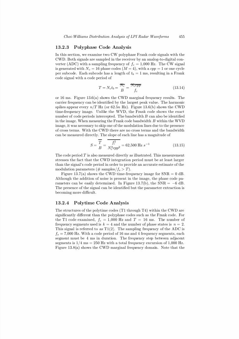
7/17/2019 1596932341 Intercept Radar.pdf
http://slidepdf.com/reader/full/1596932341-intercept-radarpdf 486/891
Choi-Williams Distribution Analysis of LPI Radar Waveforms 455
13.2.3 Polyphase Code Analysis
In this section, we examine two CW polyphase Frank code signals with the
CWD. Both signals are sampled in the receiver by an analog-to-digital con-verter (ADC) with a sampling frequency of f c = 1,000 Hz. The CW signalis generated with N c = 16 phase codes (M = 4), with a cpp = 1 or one cycleper subcode. Each subcode has a length of tb = 1 ms, resulting in a Frankcode signal with a code period of
T = N ctb = N c
B =
N ccpp
f c(13.14)
or 16 ms. Figure 13.6(a) shows the CWD marginal frequency results. Thecarrier frequency can be identified by the largest peak value. The harmonicspikes appear every n/T Hz (or 62.5n Hz). Figure 13.6(b) shows the CWDtime-frequency image. Unlike the WVD, the Frank code shows the exactnumber of code periods intercepted. The bandwidth B can also be identifiedin the image. When measuring the Frank code bandwidth B within the WVDimage, it was necessary to skip one of the modulation lines due to the presenceof cross terms. With the CWD there are no cross terms and the bandwidthcan be measured directly. The slope of each line has a magnitude of
S = T
B =
f 2cN 2c cpp2
= 62,500 Hz s−1 (13.15)
The code period T is also measured directly as illustrated. This measurementstresses the fact that the CWD integration period must be at least largerthan the signal’s code period in order to provide an accurate estimate of themodulation parameters (# samples/f s > T ).
Figure 13.7(a) shows the CWD time-frequency image for SNR = 0 dB.
Although the addition of noise is present in the image, the phase code pa-rameters can be easily determined. In Figure 13.7(b), the SNR = −6 dB.The presence of the signal can be identified but the parameter extraction isbecoming more difficult.
13.2.4 Polytime Code Analysis
The structures of the polytime codes (T1 through T4) within the CWD aresignificantly diff erent than the polyphase codes such as the Frank code. Forthe T1 code examined, f c = 1,000 Hz and T = 16 ms. The number of frequency segments used is k = 4 and the number of phase states is n = 2.This signal is referred to as T1(2). The sampling frequency of the ADC isf s = 7,000 Hz. With a code period of 16 ms and 4 frequency segments, each
segment must be 4 ms in duration. The frequency step between adjacentsegments is 1/4 ms = 250 Hz with a total frequency excursion of 1,000 Hz.Figure 13.8(a) shows the CWD marginal frequency domain. Note that the

7/17/2019 1596932341 Intercept Radar.pdf
http://slidepdf.com/reader/full/1596932341-intercept-radarpdf 487/891
456 Detecting and Classifying LPI Radar
Figure 13.6: CWD for Frank code with B = 1,000 Hz, T = 16 ms, signal only,showing (a) the marginal frequency domain plot and (b) the time-frequencyplot.
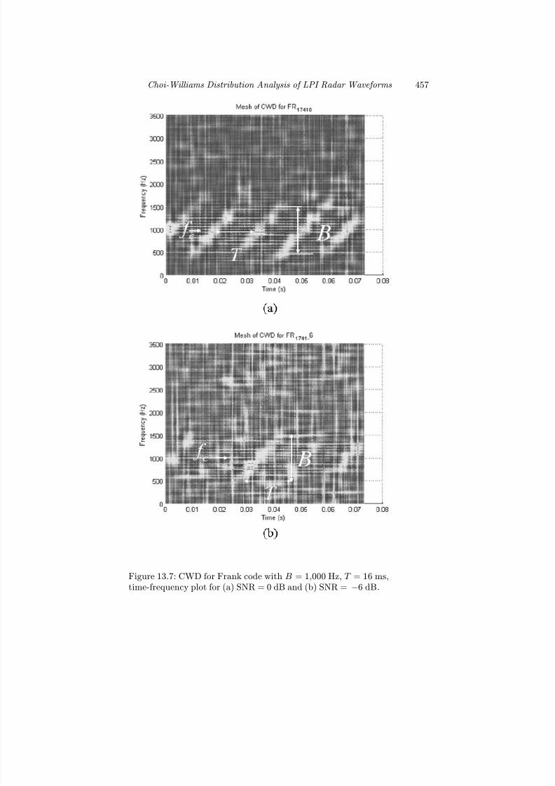
7/17/2019 1596932341 Intercept Radar.pdf
http://slidepdf.com/reader/full/1596932341-intercept-radarpdf 488/891
Choi-Williams Distribution Analysis of LPI Radar Waveforms 457
Figure 13.7: CWD for Frank code with B = 1,000 Hz, T = 16 ms,time-frequency plot for (a) SNR = 0 dB and (b) SNR = −6 dB.

7/17/2019 1596932341 Intercept Radar.pdf
http://slidepdf.com/reader/full/1596932341-intercept-radarpdf 489/891
458 Detecting and Classifying LPI Radar
harmonics are uniformly spaced due to the time modulation of the binaryphase change. Figure 13.8(b) shows the time-frequency distribution of theT1(2) code. The signal shows up as a set of vertical triangles stacked next toeach other. They are separated by the code period T . Figure 13.9(a) showsthe signal for an SNR = 0 dB. The signal can still be identified as a T1(2) andthe parameters can still be extracted. In Figure 13.9(b), with an SNR = −6dB, no signal identification can be made and no parameters can be extracted.
13.2.5 FSK and FSK/PSK Analysis
In this section, we examine the CWD results for the FSK Costas signal anda hybrid FSK/PSK signal. The CWD is used first to investigate the time-frequency characteristics of the Costas frequency hopping sequence3, 2, 6, 4, 5, 1 kHz. The signal was generated with the LPIT using a fre-quency duration of t
p = 0.005 seconds and a sampling frequency of f
s =
15,057 Hz. The CWD marginal frequency domain is shown in Figure 13.10(a).Note that the frequencies in the sequence are present and there are no crossterms, as were present in the WVD. The CWD time-frequency image is shownin Figure 13.10(b). The positions of the six Costas frequencies are shownclearly.
In Figure 13.11, the time-frequency image is displayed for both the 0-dBand −6-dB SNR signals, respectively. As expected, the identification becomesmore difficult with increasing noise levels but the presence of the signals canstill be identified. With the FSK (Costas)/PSK signal, each frequency isoverlayed with a 5-bit narrowband Barker phase code with cpp = 5 (fivecycles per phase code). The results are shown in Figure 13.12(a, b) for thesignal only, and SNR = 0 dB, respectively. The frequencies in the Costas
code can be identified along with the phase code overlay. For the FSK/PSKtarget signal described, the CWD generates excellent results and gives a clearpicture without cross terms.
13.3 Summary
The CWD theory was presented in this chapter. Several examples were usedto demonstrate generating an efficient kernel function and the subsequentcalculation of the CWD time-frequency results. The CWD was comparedto the WVD and the usefulness of the CWD to reduce the cross terms wasdemonstrated for key LPI signals. The MATLAB folder CHOI contains thefile choi.m, which can be used to generate the results in this chapter or any
other LPI waveform results.

7/17/2019 1596932341 Intercept Radar.pdf
http://slidepdf.com/reader/full/1596932341-intercept-radarpdf 490/891
Choi-Williams Distribution Analysis of LPI Radar Waveforms 459
Figure 13.8: CWD for polytime code T1(2) with B = 1,750 Hz, T = 16 ms,signal only, showing (a) the marginal frequency domain plot and (b) thetime-frequency plot.

7/17/2019 1596932341 Intercept Radar.pdf
http://slidepdf.com/reader/full/1596932341-intercept-radarpdf 491/891
460 Detecting and Classifying LPI Radar
Figure 13.9: CWD for T1(2) code with B = 1,750 Hz, T = 16 ms, time-frequency plot for (a) SNR = 0 dB and (b) SNR = −6 dB.

7/17/2019 1596932341 Intercept Radar.pdf
http://slidepdf.com/reader/full/1596932341-intercept-radarpdf 492/891
Choi-Williams Distribution Analysis of LPI Radar Waveforms 461
Figure 13.10: CWD for Costas code sequence 3, 2, 6, 4, 5, 1 kHz, showing(a) the marginal frequency domain and (b) the time-frequency image.

7/17/2019 1596932341 Intercept Radar.pdf
http://slidepdf.com/reader/full/1596932341-intercept-radarpdf 493/891
462 Detecting and Classifying LPI Radar
Figure 13.11: CWD for time-frequency image for Costas code sequence3, 2, 6, 4, 5, 1 kHz, showing (a) SNR = 0 dB and (b) SNR = −6 dB.
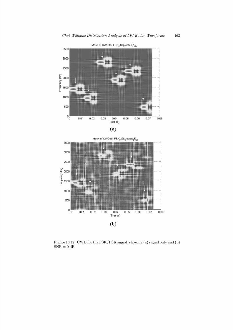
7/17/2019 1596932341 Intercept Radar.pdf
http://slidepdf.com/reader/full/1596932341-intercept-radarpdf 494/891
Choi-Williams Distribution Analysis of LPI Radar Waveforms 463
Figure 13.12: CWD for the FSK/PSK signal, showing (a) signal only and (b)SNR = 0 dB.

7/17/2019 1596932341 Intercept Radar.pdf
http://slidepdf.com/reader/full/1596932341-intercept-radarpdf 495/891
464 Detecting and Classifying LPI Radar
References
[1] Choi, H.I. and Williams W. J., ”Improved Time-Frequency Representation
of Multicomponent Signals Using Exponential Kernels,” IEEE Trans. on Acoustics, Speech, and Signal Processing , Vol. 37, No. 6, pp. 862—871, June1989.
[2] D. T. Barry, “Fast calculation of the Choi-Williams time-frequencydistribution,” IEEE Trans. on Signal Processing, Vol. 40, No. 2 pp. 450—455,Feb. 1992.
[3] Cardoso, J.C., Fish, P. J., and Ruano M. C., ”Parallel Implementation of a Choi-Williams TFD for Doppler Signal Analysis,” Proceedings of the 20th
Annual International Conference of the IEEE Engineering in Medicine and
Biology Society , Vol. 20, No. 3, 1998.
[4] Harkins, J., El-Ghazawi, T., El-Araby, E., and Huang, M., “Performanceof sorting algorithms on the SRC 6 reconfigurable computer,” Proceedings
of the IEEE International Conference on Field-Programmable Technology ,
pp. 295 - 296, 11—14 Dec. 2005.
[5] Upperman, G. J., Upperman, T. L. O., Fouts, D. J., and Pace, P. E.,“ Efficient time-frequency and bi-frequency signal processing on a reconfig-urable computer,” Proceedings of the IEEE Asilomar Conference on Signals,
Systems & Computers, 26—29 Oct. 2008.
Problems
1. Using the Choi-Williams distribution, (a) generate the time-frequencyresults for the random noise radar waveform, the random noise plusFMCW, random noise FMCW plus sine, and random binary phase mod-ulations discussed in Chapter 7. For each waveform, which modulation
parameters can be extracted from the Choi-Williams distribution?
2. Using the Choi-Williams distribution, calculate the time-frequency dis-tribution of the (a) polyphase signal that uses one of the orthogonal se-quences given in Table 10.12 (ortho40.m), (b) the polyphase signal thatuses one of the Doppler-tolerant orthogonal sequences in Table 10.14(ortho40CE.m), and (c) the frequency hopping signal that uses one of the orthogonal frequency sequences given in Table 10.16 (dfc32.m).

7/17/2019 1596932341 Intercept Radar.pdf
http://slidepdf.com/reader/full/1596932341-intercept-radarpdf 496/891
Choi-Williams Distribution Analysis of LPI Radar Waveforms 465
3. To help identify the capability of the Choi-Williams distribution asa tool for identifying the LPI modulation, extracting the modulationparameters, and to aid in deciding on what signal processing algorithmperforms best, construct a table to show the Choi-Williams measure-ment results for the LPI signals contained in the test signals folder. Foreach parameter of interest, show the actual value, the measured value,and the absolute value of the relative error [see (12.26)]. Comparedwith Wigner-Ville distribution, the absence of the cross terms shouldhelp considerably in identifying the LPI modulation and extracting themodulation parameters.

7/17/2019 1596932341 Intercept Radar.pdf
http://slidepdf.com/reader/full/1596932341-intercept-radarpdf 497/891

7/17/2019 1596932341 Intercept Radar.pdf
http://slidepdf.com/reader/full/1596932341-intercept-radarpdf 498/891
Chapter 14
LPI Radar Analysis Using
Quadrature MirrorFiltering
In Chapter 13, it was shown that the Choi-Williams distribution’s time-frequency characteristics are useful for identifying LPI waveform parametersand off ered an improvement over the Wigner-Ville analysis due to the sup-pression of the cross-terms which sometimes gave misleading results. In thischapter, we investigate an LPI intercept receiver, based on a linear decom-position of the received waveform through a quadrature mirror fi lter bank
(QMFB) tree, using wavelet filters. In this approach, the input signal is bro-ken down into a series of time-frequency layers , with each subsequent layerproviding a trade-off in time and frequency resolution.
By examining the correct layers, the QMFB time-frequency receiver ap-proach provides good estimates of the LPI signal parameters, making it easyto distinguish between the diff erent modulations, and extract the parametervalues. Parameters such as bandwidth, center frequency, energy distributionwithin a tile (region in the time-frequency plane that contains most of thewavelet basis function’s energy), phase modulation, signal duration, and loca-tion in the time-frequency plane can be determined. In addition, the numberof transmitters present and the types of LPI emitters can be determined. Inthis chapter, the QMFB theory is presented first, followed by a discussionof the mathematical waveform decomposition using wavelets. The QMFB is
then used to analyze and extract the parameters for the LPI signals discussedin Part I. The QMFB folder on the CD provides the MATLAB tools that canbe used to re-create any of the figures presented, as well as generate new anduseful results.
467

7/17/2019 1596932341 Intercept Radar.pdf
http://slidepdf.com/reader/full/1596932341-intercept-radarpdf 499/891
468 Detecting and Classifying LPI Radar
14.1 Time-Frequency WaveletDecomposition
Various methods of decomposing a waveform on the time-frequency planehave recently been investigated. The most common methods use orthogonalbasis functions, and can be divided into linear and bilinear transforms. Theshort-time Fourier transform (STFT) and the wavelet transform (WT) areexamples of linear transforms. The Wigner transform discussed in the previ-ous chapter is an example of a bilinear transform.1 After a discussion of basisfunctions, the STFT and the WT are discussed, along with their advantagesand limitations.
14.1.1 Basis FunctionsLinear transforms of a continuous time signal f (t) have the following form
ak =
f (t)Φk(t)dt (14.1)
where Φ(t) is the basis set, t is the time index, and k is the function index.The Fourier transform, for example, has a basis set consisting of sines andcosines of frequency 2πk that oscillate forever. The basis functions are saidto be orthogonal if
Φ(t)Φ(t− k) = E δ (k) =
E if k = 00 otherwise
(14.2)
where E stands for the energy of Φ(t) [1]. If Φ(t) is normalized by dividingby the square root of the energy
√ E , then the basis functions are said to be
orthonormal defined by [2]
Φ(t)Φ(t− k)dt = δ (k) =
1 if k = 00 otherwise
(14.3)
If the basis functions are orthonormal, there is no redundancy in the repre-sentation of the signal f (t). If the signal is sampled at or above the Nyquistrate, all of the signal’s information is retained. In this case, the time variablet in (14.1) and (14.3) can be considered to be discrete t = nT where T is thesampling period and the integral should be replaced with summations.
1Wigner transforms are called bilinear because the input waveform appears twice in the
development of the transform. Better resolution occurs in the time-frequency plane than
with linear techniques; however, the computational burden is greatly increased and the
cross terms can be bothersome for some applications.

7/17/2019 1596932341 Intercept Radar.pdf
http://slidepdf.com/reader/full/1596932341-intercept-radarpdf 500/891
LPI Radar Analysis Using Quadrature Mirror Filtering 469
14.1.2 Short-Time Fourier Transform DecompositionThe Fourier transform uses complex sinusoids as basis functions to performthe analysis of signals. This approach is difficult, due to the infinite extent of the basis functions as any time-local information (such as an abrupt changein the signal) is spread out over the entire frequency axis [3]. This problemwas addressed by Gabor by introducing windowed complex sinusoids as basisfunctions. This leads to the doubly indexed windowed Fourier transform:
X WF (ω, τ ) =
∞
−∞
e−jωtw(t− τ )x(t)dt (14.4)
where w(t − τ ) constitutes an appropriate window, and X WF (ω, τ ) is theFourier transform of x(t) windowed with w(·) shifted by τ . The function of the window is to extract a finite-length portion of the signal x(t) such that thespectral characteristics of the section extracted are approximately stationaryover the duration of the window. Also, if w(t) = 1 then the STFT reduces tothe conventional Fourier transform of x(t). In most applications, the magni-tude of the STFT is of interest, and the display of the STFT magnitude isusually referred to as a spectrogram [4].
The major advantage of the windowed transform or STFT is that if asignal has most of its energy in a given time interval [−T, T ] and frequencyinterval [−Ω,Ω], then its STFT will be localized in the region [−T, T ]×[−Ω,Ω]and will be close to zero in time and frequency intervals, where the signal haslittle energy [3]. A limitation of the STFT is that, because a single windowis used for all frequencies, the resolution of the analysis is the same at all
locations in the time-frequency plane. The possibility of having arbitrarilyhigh resolution in both time and frequency is thus excluded.
14.1.3 Wavelets and the Wavelet Transform
Wavelets are localized basis functions for time-frequency analysis of a signal.That is, the wavelet basis function is eff ectively nonzero for only a finitetime interval, and is designed to satisfy the orthonormality condition (14.3).From a signal processing point of view, a wavelet is a bandpass filter. Inthe time-frequency analysis, the wavelet filter occurs most often in pairs (alowpass filter and a highpass filter), and includes a resampling function thatis coupled to the filter bandwidth as shown in the two-band analysis bankin Figure 14.1. Here, H 0(z) is the highpass filter and H 1(z) is the lowpass
filter. Like the design of conventional digital filters, the design of a waveletfilter can be accomplished by using a number of methods including weightedleast squares [5, 6], orthogonal matrix methods [7], nonlinear optimization,optimization of a single parameter (e.g., the passband edge) [8], and a methodthat minimizes an objective function that bounds the out-of-tile energy [9].
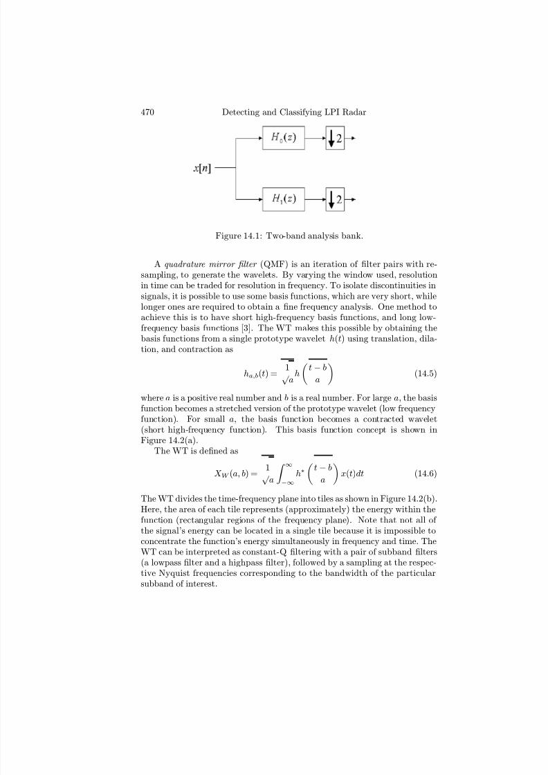
7/17/2019 1596932341 Intercept Radar.pdf
http://slidepdf.com/reader/full/1596932341-intercept-radarpdf 501/891
470 Detecting and Classifying LPI Radar
Figure 14.1: Two-band analysis bank.
A quadrature mirror fi lter (QMF) is an iteration of filter pairs with re-
sampling, to generate the wavelets. By varying the window used, resolutionin time can be traded for resolution in frequency. To isolate discontinuities insignals, it is possible to use some basis functions, which are very short, whilelonger ones are required to obtain a fine frequency analysis. One method toachieve this is to have short high-frequency basis functions, and long low-frequency basis functions [3]. The WT makes this possible by obtaining thebasis functions from a single prototype wavelet h(t) using translation, dila-tion, and contraction as
ha,b(t) = 1√
ah
t− b
a
(14.5)
where a is a positive real number and b is a real number. For large a, the basis
function becomes a stretched version of the prototype wavelet (low frequencyfunction). For small a, the basis function becomes a contracted wavelet(short high-frequency function). This basis function concept is shown inFigure 14.2(a).
The WT is defined as
X W (a, b) = 1√
a
∞
−∞
h∗
t− b
a
x(t)dt (14.6)
The WT divides the time-frequency plane into tiles as shown in Figure 14.2(b).Here, the area of each tile represents (approximately) the energy within thefunction (rectangular regions of the frequency plane). Note that not all of the signal’s energy can be located in a single tile because it is impossible to
concentrate the function’s energy simultaneously in frequency and time. TheWT can be interpreted as constant-Q filtering with a pair of subband filters(a lowpass filter and a highpass filter), followed by a sampling at the respec-tive Nyquist frequencies corresponding to the bandwidth of the particularsubband of interest.

7/17/2019 1596932341 Intercept Radar.pdf
http://slidepdf.com/reader/full/1596932341-intercept-radarpdf 502/891
LPI Radar Analysis Using Quadrature Mirror Filtering 471
Figure 14.2: Basis functions and time-frequency resolution of the wavelettransform: (a) basis functions and (b) coverage of time-frequency plane [3]( cIEEE 1992).

7/17/2019 1596932341 Intercept Radar.pdf
http://slidepdf.com/reader/full/1596932341-intercept-radarpdf 503/891
472 Detecting and Classifying LPI Radar
Figure 14.3: Haar lowpass FIR fi
lter.
14.1.4 Wavelet Filters
Finite impulse response (FIR) filters are the popular choice for the waveletfilter. To meet the requirements for a wavelet filter, the coefficients mustensure an orthogonal decomposition of the input signal, such that the energyat the input will equal the energy at the output from each filter pair [10]. Thefilter pairs are designed to divide the input signal energy into two orthogonalcomponents based on the frequency. The filter should also pass as muchenergy within its tile with a flat passband, and reject as much energy outsidethe tile as possible.
Haar Filter
A classic example of a wavelet filter is the Haar basis function, which is notcontinuous but is of interest because of its simplicity. The Haar basis functionis
h(t) =
⎧⎨⎩
1 for 0 ≤ t < 1/2−1 for 1/2 ≤ t < 10 otherwise
(14.7)
and is shown in Figure 14.3. The Haar basis function can serve as a waveletlowpass FIR filter and has two coefficients, both with values of 1/2. TheHaar filter meets the wavelet requirements with the orthonormality beingeasily verified since, at a given scale, the translations are nonoverlapping [3].Because of the scale change by 2, the basis functions are orthonormal across
scale. Unfortunately, the Haar function is discontinuous. Although the filtermeets the wavelet requirements and perfectly tiles the input energy in time,it does not tile well in frequency, and is not appropriate for signal processing.Consequently, a continuous set of basis functions (or filters) is needed that

7/17/2019 1596932341 Intercept Radar.pdf
http://slidepdf.com/reader/full/1596932341-intercept-radarpdf 504/891
LPI Radar Analysis Using Quadrature Mirror Filtering 473
Figure 14.4: Sampled sinc filter impulse response.
best approximates the perfect time-frequency tiling, by minimizing the out-of-time and out-of-frequency energy.
Sinc and Modified Sinc Filter
A function that tiles the energy perfectly in frequency would have a flatmagnitude response across the passband, an infinitely narrow passband-to-stopband transition, and a zero across the stopband. From the time-domaindescription (inverse Fourier transform), the function is called a sinc fi lter .While it has an infinite number of coefficients, this condition can be modified
by windowing [11]. The sinc fi
lter can be expressed as
sinc(k) =
sin(πk)
πk k = 0
1 k = 0 (14.8)
Since the passband ranges from −π/2 < ω < π/2 or −0.25 < f < 0.25, thenulls of the sinc function will be at 2T for a sampling period of T [12]. Toobtain the filter coefficients, the sinc function is sampled at the normalizedsampling period of T = 1 for a situation similar to that shown in Figure 14.4.One way to sample the function would be to let the main tap sample occurat the center of the main lobe. However, two main taps are needed, and theirsum needs to be as large as possible. This occurs for the sinc function if bothmain tap samples are equally spaced about the center of the main lobe [10].The sum of the square of the coefficients must be unity also, which is achievedby scaling the sinc by 1/√ 2, giving
h(n) = 1√
2sinc
n + 0.5
2
(14.9)
where n is an integer.

7/17/2019 1596932341 Intercept Radar.pdf
http://slidepdf.com/reader/full/1596932341-intercept-radarpdf 505/891
474 Detecting and Classifying LPI Radar
This filter meets the criteria of wavelet filters. The only problem isthat there is an infinite number of coefficients. A small amount of non-orthogonality will occur when this filter is truncated. Some cross correlationwill also take place between both highpass and lowpass filters. If the ends of the filter are simply truncated (a rectangular window in the time domain),some ripples in the passband of the frequency response will appear (Gibb’sphenomena).
One solution is to use a nonrectangular window, and one whose Fouriertransform has a narrower main lobe and smaller side lobes than the sincfunction. The Hamming window is one that is commonly used. Multiplyingthe coefficients from (14.9) by this window, and using the results in an FIRfilter, the frequency response needed is generated. Energy will be lost at thefilter transitions, which is primarily the result of the loss of orthogonalityfrom truncating the filter [11].
For detection, instead of losing the energy at those frequencies, a bettertrade-off would be a small amount of cross correlation between the filters,so that some energy appears in more than one tile. To achieve this type of prototype filter, the impulse response can be modified to have a passbandthat is slightly greater than π/2. Thus, the lowpass and highpass filtersare squeezed together slightly. This can be achieved by compressing thesinc envelope of (14.9) slightly. At the same time, it is desirable to rescalethe coefficients slightly, so the sum of the squares equals one. With thesemodifications, a modi fi ed sinc fi lter results as [9, 10]
h(n) = S
2
sincn + 0.5
C w(n) (14.10)
where −N/2 ≤ n ≤ (N − 2)/2, C is the compression variable, S is thescaling variable, N is the number of coefficients, and w(n) is the Hammingwindow to suppress the Gibb’s phenomena. For these filters, the greatestcross correlation occurs between tiles in the same frequency band, and ad-
jacent in time, when N = 512 (the number of coefficients), with valuesC = 1.99375872328059, S = 1.00618488680080, and a Hamming window witha cross correlation of less than 0.001 results.2 Note the number of coefficientsN can be changed using the MATLAB file tsinc su.m.
14.2 Discrete Two-Channel
Quadrature Mirror Filter BankDigital two-channel QMFB structures have found applications in many areas,including modems, data transmission, image, and video coding. Figure 14.5
2Personal communication between P. Jarpa and T. Farrell, March 20, 2002.

7/17/2019 1596932341 Intercept Radar.pdf
http://slidepdf.com/reader/full/1596932341-intercept-radarpdf 506/891
LPI Radar Analysis Using Quadrature Mirror Filtering 475
Figure 14.5: Two-channel quadrature mirror filter bank [5] ( cIEEE 2000).
Figure 14.6: Typical frequency response of the analysis filters.
shows the basic two-channel QMFB structure consisting of an analysis filterbank and a synthesis filter bank. In the two-channel analysis filter bank, adiscrete time signal x[n] is first split into two subbands vk[n] by means of thewavelet or analysis filters H 0(z) and H 1(z). The two-band analysis filter bankcontaining the filters H 0(z) and H 1(z) typically have lowpass and mirror-image highpass frequency responses, respectively, with a cutoff frequency atπ/2 [5, 13]. The typical frequency response of the analysis filters is shownin Figure 14.6. After filtering, each subband signal is downsampled by 2, toform the outputs of the analysis stage. These signals can then be analyzedor processed in various ways, depending on the application. The signalsare then transmitted to the “signal synthesis section,” where the signals areupsampled by a factor of 2, and passed through a two-band synthesis filterbank composed of the filters G0(z) and G1(z), whose outputs are then addedyielding y[n]. The purpose of the synthesis filters is to eliminate the images
that are formed in the analysis stage.It follows from the figure that the sampling rates of the input signal x[n]and output signal y[n] are the same. The reconstructed signal y(n) diff ers,however, from the input x(n) due to aliasing, amplitude distortion, and phasedistortion [5, 13]. Consequently, the analysis and the synthesis filters in theQMFB are chosen so as to ensure that the reconstructed output y[n] is a
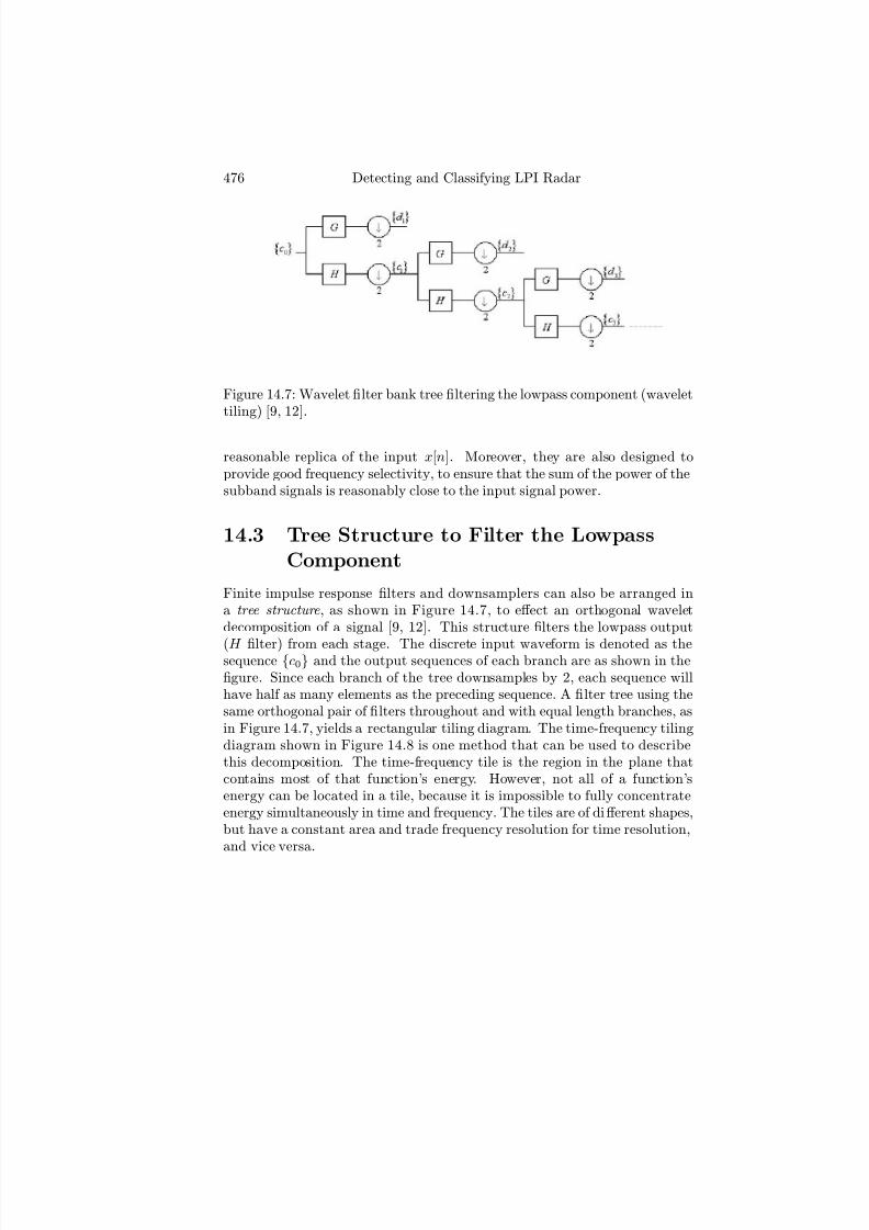
7/17/2019 1596932341 Intercept Radar.pdf
http://slidepdf.com/reader/full/1596932341-intercept-radarpdf 507/891
476 Detecting and Classifying LPI Radar
Figure 14.7: Wavelet filter bank tree filtering the lowpass component (wavelettiling) [9, 12].
reasonable replica of the input x[n]. Moreover, they are also designed toprovide good frequency selectivity, to ensure that the sum of the power of thesubband signals is reasonably close to the input signal power.
14.3 Tree Structure to Filter the LowpassComponent
Finite impulse response filters and downsamplers can also be arranged ina tree structure , as shown in Figure 14.7, to eff ect an orthogonal waveletdecomposition of a signal [9, 12]. This structure filters the lowpass output
(H filter) from each stage. The discrete input waveform is denoted as thesequence c0 and the output sequences of each branch are as shown in thefigure. Since each branch of the tree downsamples by 2, each sequence willhave half as many elements as the preceding sequence. A filter tree using thesame orthogonal pair of filters throughout and with equal length branches, asin Figure 14.7, yields a rectangular tiling diagram. The time-frequency tilingdiagram shown in Figure 14.8 is one method that can be used to describethis decomposition. The time-frequency tile is the region in the plane thatcontains most of that function’s energy. However, not all of a function’senergy can be located in a tile, because it is impossible to fully concentrateenergy simultaneously in time and frequency. The tiles are of diff erent shapes,but have a constant area and trade frequency resolution for time resolution,and vice versa.

7/17/2019 1596932341 Intercept Radar.pdf
http://slidepdf.com/reader/full/1596932341-intercept-radarpdf 508/891
LPI Radar Analysis Using Quadrature Mirror Filtering 477
Figure 14.8: Time-frequency diagram for the lowpass wavelet filter bank tree[9] ( cIEEE 1999).
Figure 14.9: Wavelet filter bank tree filtering the highpass component.
14.4 Tree Structure to Filter the HighpassComponent
The last section demonstrated that by cascading filters and filtering the low-pass component of the previous output, a tiling with finer frequency resolutionat lower frequencies was achieved. Now consider the cascading filter diagramin Figure 14.9 where, instead of filtering the lowpass output of each stage, thehighpass filter (G filter) output is filtered. Again, the input sequence is splitat each stage into high-frequency and low-frequency orthogonal sequences.
The tiling diagram is shown in Figure 14.10.Notice that the second and third layers seem to be flipped in Figure 14.9.
The figure is drawn so that the output sequence at the top of the drawingcontains the highest frequency components of the input sequence. To un-derstand why they are flipped, consider the aliased frequency spectrum of

7/17/2019 1596932341 Intercept Radar.pdf
http://slidepdf.com/reader/full/1596932341-intercept-radarpdf 509/891
478 Detecting and Classifying LPI Radar
Figure 14.10: Time-frequency diagram for the highpass wavelet filter banktree.
the filters, shown in Figure 14.11. The output from the G filter in the firstlayer contains the higher frequency components of the original sequence, butshifted, so that it is actually the dc component of the output of G. The resultis that the output of G is frequency reversed, much like the lower sideband of a single sideband communication system. A similar structure farther downthe cascade will unflip the signal.
It is possible to create another tiling scheme by combining the waveletfilter bank and wavelet tiling, as demonstrated in Figure 14.12. In order tokeep the higher frequency outputs of each branch above the lower frequency
outputs, the construction rule for this figure is to count the number of Gfilters up to the branch. If the number is even, the next G filter will outputthe high frequencies. If odd, the next H filter will output the high frequencies.
14.5 QMFB Tree Receiver
Orthogonal wavelet decomposition of the unknown signal can be implementedusing QMFs, by designing filter pairs to divide the input signal energy into twoorthogonal components, based on frequency. The tiles are used to refer to therectangular regions of the time-frequency plane containing the basis function’senergy. By arranging the QMF pairs in a fully developed tree structure, itis possible to decompose the waveform in such a way that the tiles have the
same dimensions within each layer. Thus, every fi
lter output is connected toa QMF pair in the next layer, as shown in Figure 14.13 [10]. Each QMF pairdivides the digital input waveform into its high-frequency and low-frequencycomponents, with a transition centered at π. A normalized input of onesample per second is assumed, with a signal bandwidth of [0, π]. Since eachfilter output signal has half the bandwidth, only half the samples are required

7/17/2019 1596932341 Intercept Radar.pdf
http://slidepdf.com/reader/full/1596932341-intercept-radarpdf 510/891
LPI Radar Analysis Using Quadrature Mirror Filtering 479
Figure 14.11: Frequency response of filters H and G.
to meet the Nyquist criteria; therefore, these sequences are downsampled bytwo. The same number of output samples is returned. For example, if 100samples appear at the input of the first QMF pair, 100 samples appear atthe output. Each of the two resulting sequences is then fed into QMF pairs,forming the next layer, where the process is repeated, and so on down the
tree.Within the time-frequency plane, the WT is sharper in time at high fre-
quencies. At low frequencies, the WT is sharper in frequency. That is, thetiles become shorter in time and occupy a larger frequency band, as the fre-quency is increased. Since the WT is linear, there is a fundamental limit onthe minimum area of these tiles. However, the nature of the QMFB config-uration is such that each layer outputs a matrix of coefficients for tiles thatare twice as long (in time) and half as tall (in frequency) as the tile in theprevious layer. The outputs from each layer of the tree in Figure 14.13 forma matrix whose elements, when squared, approximately represent the energycontained in the tiles of the corresponding time-frequency diagrams shown inthe figure.
The block diagram of a receiver that uses the QMFB structure is shown
in Figure 14.14. A received waveform is bandpass filtered and sampled at theNyquist rate. The digital sequence is then fed to the QMFB tree where itis decomposed. Matrices of values are output from each layer, and are thensquared to produce numbers representing the energy in each tile.
Wavelet decomposition has been investigated as a tool for pattern recogni-
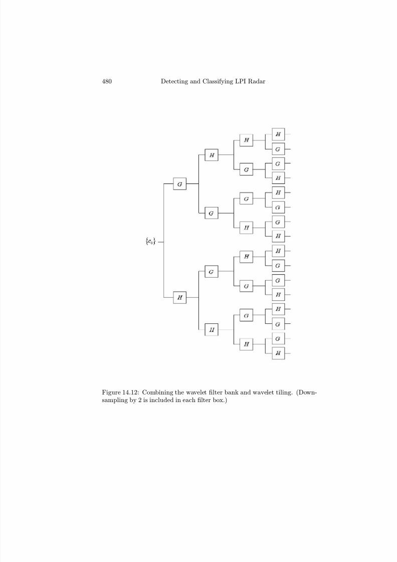
7/17/2019 1596932341 Intercept Radar.pdf
http://slidepdf.com/reader/full/1596932341-intercept-radarpdf 511/891
480 Detecting and Classifying LPI Radar
Figure 14.12: Combining the wavelet filter bank and wavelet tiling. (Down-sampling by 2 is included in each filter box.)
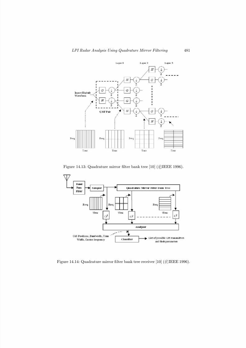
7/17/2019 1596932341 Intercept Radar.pdf
http://slidepdf.com/reader/full/1596932341-intercept-radarpdf 512/891
LPI Radar Analysis Using Quadrature Mirror Filtering 481
Figure 14.13: Quadrature mirror filter bank tree [10] ( cIEEE 1996).
Figure 14.14: Quadrature mirror filter bank tree receiver [10] ( cIEEE 1996).

7/17/2019 1596932341 Intercept Radar.pdf
http://slidepdf.com/reader/full/1596932341-intercept-radarpdf 513/891
482 Detecting and Classifying LPI Radar
tion and target detection [14], and also as a means for identifying signal mod-ulations [15]. The architecture discussed above has been used to investigatethe detection of LPI signals in [16—19], and is used below to investigate theparameters of the signals in Part I. We start with two example calculations,to become familiar with the QMFB processing and its output waveforms.
14.6 Example Calculations
In this section two example calculations are shown for a complex input. Acomplex single-tone example is shown first, followed by a two-tone signal.These examples serve to demonstrate the diff erent QMFB output layers, andshow the trade-off in time-frequency resolution as a function of the layer
number being examined. The lower the layer number, the smaller (better)the resolution in time, and consequently the larger (poorer) the resolution infrequency. As the layer number gets larger, the resolution in time gets larger,and the resolution in frequency gets smaller.
14.6.1 Complex Single-Tone Signal
To demonstrate the results available from the QMFB signal processing, weagain consider a complex, single-tone signal as in Chapter 9. The signal hasa carrier frequency f c = 1 kHz and is sampled by the ADC at a rate of 7 kHz.The results, shown in Figure 14.15 show layers 2, 3, and 4, respectively, inthe time-frequency domain using gray scale plots. Figure 14.16(a, b), showlayers 5 and 6. One of the important objectives of showing the five layers
of the QMFB is to demonstrate how each layer results in a matrix of energy values, and the fact that the tiles are twice as long (in time) and half as tall(in frequency) as the tile in the previous layer . That is, as the layer numberincreases, the frequency resolution gets smaller, and the time resolution getslarger. This adds quite a bit of flexibility to the analysis of nonstationarysignals. Several diff erent layers can be examined and compared, and theparameters of the signals can be extracted with high fidelity. Also, since thefirst and last layer in the QMFB are a single row of data, it is not useful todisplay them in a time-frequency format.
The input signal is zero padded with z zeros, such that the resultingnumber of data points is a power of 2. This resulting power of 2 is the numberof layers L within the QMFB that result. That is, N p = 2L. The QMFBoutput resolution depends on the layer number. The frequency resolution of
a layer l is [19]
∆f = f s
2(2l − 1) =
f s2(N F )
(14.11)
where N F is the number of tiles displayed in frequency. For example, for layer2 in Figure 14.15, ∆f = 7,000/2(3) = 1,166.67 Hz. The resolution in time is

7/17/2019 1596932341 Intercept Radar.pdf
http://slidepdf.com/reader/full/1596932341-intercept-radarpdf 514/891
LPI Radar Analysis Using Quadrature Mirror Filtering 483
Figure 14.15: Time-frequency layers for the 1-kHz single-tone signal, showing(a) layer 2, (b) layer 3, and (c) layer 4.

7/17/2019 1596932341 Intercept Radar.pdf
http://slidepdf.com/reader/full/1596932341-intercept-radarpdf 515/891
484 Detecting and Classifying LPI Radar
Figure 14.16: Time-frequency layers for the 1-kHz single-tone signal, showing(a) layer 5, and (b) layer 6.

7/17/2019 1596932341 Intercept Radar.pdf
http://slidepdf.com/reader/full/1596932341-intercept-radarpdf 516/891
LPI Radar Analysis Using Quadrature Mirror Filtering 485
determined by how many samples are integrated within the QMFB. For layerl < L,
∆t = N p
f s(2L−l − 1) =
N pf sN T
(14.12)
where L is the total number of layers, and N T is the number of tiles intime. Also, N p = 2L. For example, for layer 2 in Figure 14.15, ∆t = 128(1/7,000)/31 = 590 μs. Also note that the lower layers (e.g., layers 2 and3) can be used to identify how many samples of the signal were collected(excluding zero padding). Since the sampling period for this example is T =0.143 ms, from layer 2 we see that 105 samples were collected, and that 23zeros were used to pad the signal.
Referring to layer l = 6 in Figure 14.16(b), the tiles have a frequency
resolution of ∆
f = 55.5556 Hz and a resolution in time of ∆
t = 18.286 ms.Layer 6 shows the signal between 944.445 Hz and 1055.56 Hz, and from 0 to18.286 ms. That is, we can say that f c ≈ 1,000 Hz with the accuracy limitedby the tile resolution. Note that if more detailed time information is required,a lower layer could be examined.
14.6.2 Complex Two-Tone Signal
The second example consists of a signal with two frequencies f c1 = 1 kHzand f c2 = 2 kHz, with a sampling frequency f s = 7 kHz. In this example, acontour plot is used. Although the gray scale plot illustrated above quantifiesthe energy within each tile, the contour plot is useful for other types of in-formation (such as time-domain characteristics), as illustrated in the results
below. The number of signal samples collected, the time resolution ∆t, andfrequency resolution ∆f for each layer within the QMFB are the same as forthe single-tone example above. Figure 14.17 shows the contour plot for layers2 through 4. Figure 14.18 shows the contour plot for layers 5 and 6. As be-fore, layers 1 and 7 are not displayed, since they have only a single row vectorof data. This example illustrates the important concepts that are evidentusing a contour image. First, for lower layers such as layer 2 and layer 3, thetime domain characteristics of the signals can be clearly identified. In layer 2,the complex phase interaction in time, of the two signals within a single filter,can also be identified. The high-frequency resolution layers [such as layer 6shown in Figure 14.18(b)] reveal the frequencies contained in the input signalwith a good amount of accuracy (∆f = 55 Hz).

7/17/2019 1596932341 Intercept Radar.pdf
http://slidepdf.com/reader/full/1596932341-intercept-radarpdf 517/891
486 Detecting and Classifying LPI Radar
Figure 14.17: Time-frequency layers for the two-tone signal (1 kHz, 2 kHz),showing (a) layer 2, (b) layer 3, and (c) layer 4.

7/17/2019 1596932341 Intercept Radar.pdf
http://slidepdf.com/reader/full/1596932341-intercept-radarpdf 518/891
LPI Radar Analysis Using Quadrature Mirror Filtering 487
Figure 14.18: Time-frequency layers for the two-tone signal (1 kHz, 2 kHz),showing (a) layer 5, and (b) layer 6.
14.7 FMCW Analysis
In this section, the extraction of FMCW signal parameters (discussed inChapter 4) is demonstrated using the QMFB, and the appropriate layersfor parameter extraction are identified.
The first example is shown in Figure 14.19. In Figure 14.19(a), the l = 2layer is shown. For the number of signal samples collected, L = 11 (N p =2, 048). For layer l = 2, ∆f = 1,166.67 Hz and ∆t = 572.5 μs. For thissignal, it appears that four periods of the triangular FMCW waveform werecaptured. The waveforms also have the general appearance of a linear FMmodulation. The modulation period tm can be measured as tm = 20 ms, for atotal signal length of 160 ms. Notice that the concentrations of energy withineach period of the FMCW waveform are not centered on the carrier frequencyf c = 1,000 Hz, but contain a 300-Hz bias. This is due to the fact that thereare only three filters in this layer being used to calculate the results.
In Figure 14.19(b), layer l = 6 is shown with ∆
f = 55.55 Hz and ∆
t =8.866 ms. This layer is appropriate, since the time resolution ∆t < tm/2. Notethat the modulation period can be easily identified and measured. Since thislayer also has 63 filters, each with a narrow filter width, the bandwidth ∆F can be measured with good accuracy, as ∆F = 250 Hz.
Figure 14.20 shows the QMFB layer 5 performance against the FMCW

7/17/2019 1596932341 Intercept Radar.pdf
http://slidepdf.com/reader/full/1596932341-intercept-radarpdf 519/891
488 Detecting and Classifying LPI Radar
Figure 14.19: QMFB contour images for FMCW ∆F = 250 MHz, tm =20 ms (signal only), showing (a) layer 2, and (b) layer 6.
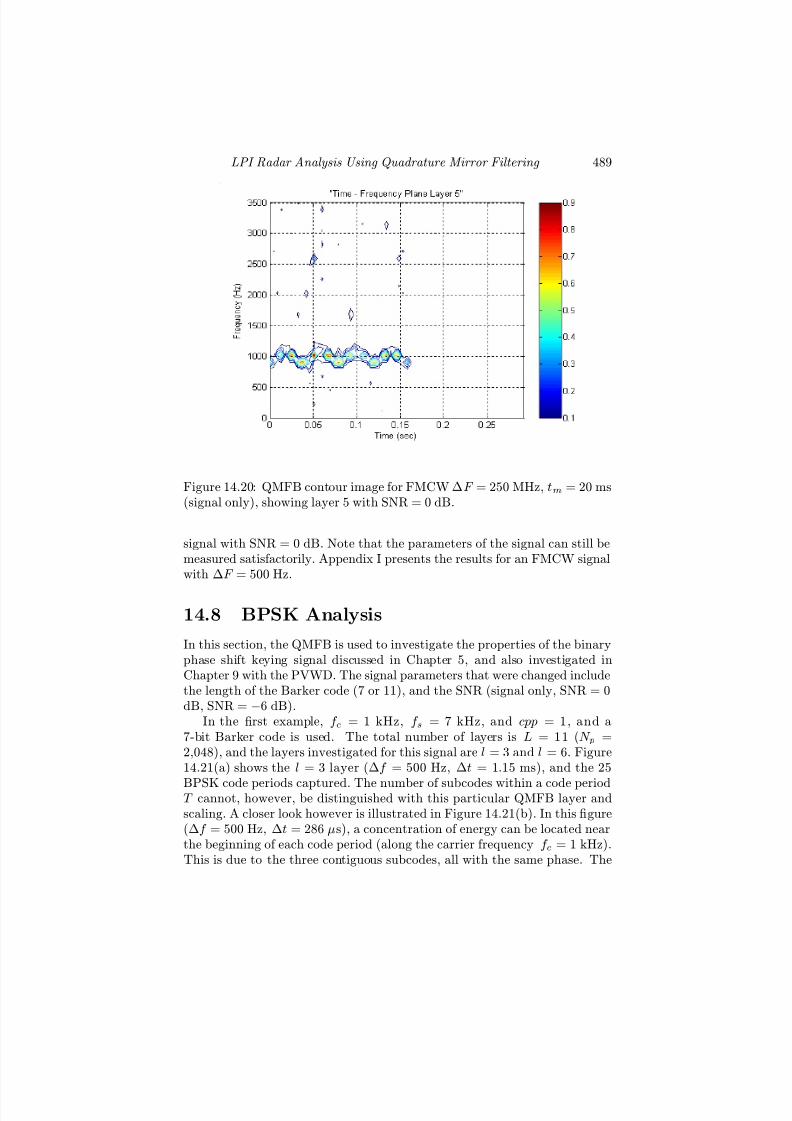
7/17/2019 1596932341 Intercept Radar.pdf
http://slidepdf.com/reader/full/1596932341-intercept-radarpdf 520/891
LPI Radar Analysis Using Quadrature Mirror Filtering 489
Figure 14.20: QMFB contour image for FMCW ∆F = 250 MHz, tm = 20 ms(signal only), showing layer 5 with SNR = 0 dB.
signal with SNR = 0 dB. Note that the parameters of the signal can still bemeasured satisfactorily. Appendix I presents the results for an FMCW signalwith ∆F = 500 Hz.
14.8 BPSK Analysis
In this section, the QMFB is used to investigate the properties of the binaryphase shift keying signal discussed in Chapter 5, and also investigated inChapter 9 with the PVWD. The signal parameters that were changed includethe length of the Barker code (7 or 11), and the SNR (signal only, SNR = 0dB, SNR = −6 dB).
In the first example, f c = 1 kHz, f s = 7 kHz, and cpp = 1, and a7-bit Barker code is used. The total number of layers is L = 11 (N p =2,048), and the layers investigated for this signal are l = 3 and l = 6. Figure14.21(a) shows the l = 3 layer (∆f = 500 Hz, ∆t = 1.15 ms), and the 25
BPSK code periods captured. The number of subcodes within a code periodT cannot, however, be distinguished with this particular QMFB layer andscaling. A closer look however is illustrated in Figure 14.21(b). In this figure(∆f = 500 Hz, ∆t = 286 μs), a concentration of energy can be located nearthe beginning of each code period (along the carrier frequency f c = 1 kHz).This is due to the three contiguous subcodes, all with the same phase. The

7/17/2019 1596932341 Intercept Radar.pdf
http://slidepdf.com/reader/full/1596932341-intercept-radarpdf 521/891
490 Detecting and Classifying LPI Radar
code period can be measured between these energy concentrations as T = 7ms. Note that care must be exercised in this measurement, since a secondaryfeature could be used, resulting in T ≈ 14 ms. The total length of the signalis 25 times 7 ms = 0.175s and can also be identified in Figure 14.21(a).
Figure 14.22(a) examines the l = 6 layer (∆f = 55 Hz, ∆t = 9.44 ms)to further evaluate the frequency content of the signal at a higher resolution.The first important feature is the frequency bands, due to the various lengthsof subcode groups within the code period. The overall bandwidth of the signalB = f c/cpp is also shown, and depends on the length of a single subcode.Figure 14.22(b) shows the same layer 6, except that the SNR = 0 dB, anddemonstrates the eff ects of noise on the QMFB output.
To further illustrate the QMFB capability to analyze the microstructureof the phase-modulated signal, cpp is increased from 1 to 5. That is, thebandwidth of the signal is narrowed from 1 kHz to B = f c/cpp = 0.2 kHz(code period of T = cpp/f c = 35 ms). Figure 14.23(a) shows the QMFB layer2 for two code periods of the 7-bit signal. The important feature illustratedhere is the presence of a null at each BPSK phase shift. After the totalcode period T is determined, the measurement of the smallest subphasecode is performed (time is measured between the two closest nulls). Afterthis, the number of subphase codes contained within each section of the codeis determined, which then uniquely identifies which BPSK code has beenintercepted. Figure 14.23(b) shows the QMFB layer 6. Note that the codeperiod T is clearly identified, as well as the bandwidth. The QMFB resultsfor an 11-bit code are shown in Appendix J.
Figure 14.24 shows the QMFB layer 6 performance against the BPSK sig-
nal, with SNR = 0 dB and cpp = 5. The parameters of the signal such as thecode period, carrier frequency, and bandwidth, can still be measured satis-factorily. For layer 2, however, the noise severely distorts the time-frequencyresults, and identification of the phase nulls is not possible, making it dif-ficult to identify the exact binary phase code used, without further imageprocessing.

7/17/2019 1596932341 Intercept Radar.pdf
http://slidepdf.com/reader/full/1596932341-intercept-radarpdf 522/891
LPI Radar Analysis Using Quadrature Mirror Filtering 491
Figure 14.21: QMFB layer 3 contour plot for BPSK with 7-bit Barker code,cpp = 1 (signal only), showing (a) the complete captured signal, and (b) aclose-up view showing the code period T = 7 ms.
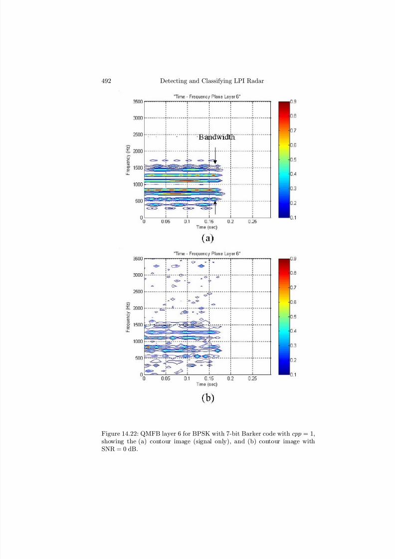
7/17/2019 1596932341 Intercept Radar.pdf
http://slidepdf.com/reader/full/1596932341-intercept-radarpdf 523/891
492 Detecting and Classifying LPI Radar
Figure 14.22: QMFB layer 6 for BPSK with 7-bit Barker code with cpp = 1,showing the (a) contour image (signal only), and (b) contour image withSNR = 0 dB.
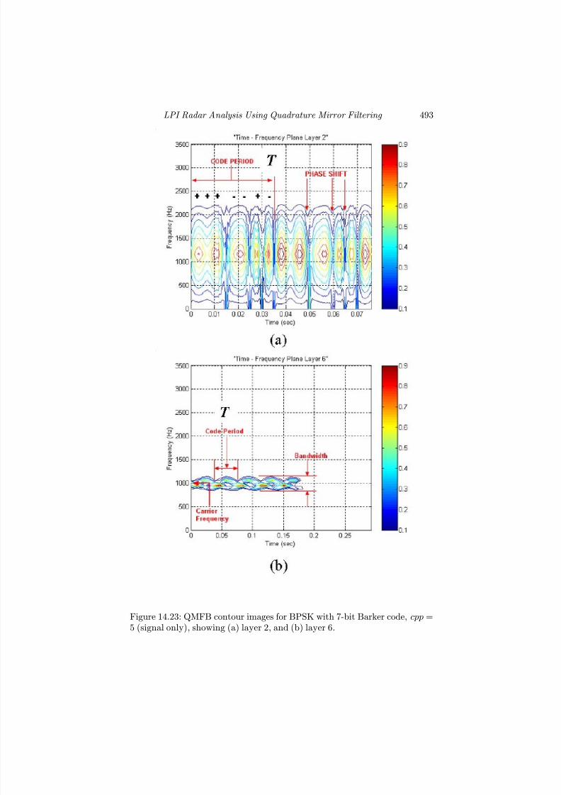
7/17/2019 1596932341 Intercept Radar.pdf
http://slidepdf.com/reader/full/1596932341-intercept-radarpdf 524/891
LPI Radar Analysis Using Quadrature Mirror Filtering 493
Figure 14.23: QMFB contour images for BPSK with 7-bit Barker code, cpp =5 (signal only), showing (a) layer 2, and (b) layer 6.

7/17/2019 1596932341 Intercept Radar.pdf
http://slidepdf.com/reader/full/1596932341-intercept-radarpdf 525/891
494 Detecting and Classifying LPI Radar
Figure 14.24: QMFB layer 6 contour image for BPSK cpp = 5 signal, withSNR = 0 dB.
14.9 Polyphase Code Analysis
In this section we examine the polyphase codes with the QMFB, beginning
with the Frank code. In Chapter 5 we saw that the Frank code is derived froma linear FM waveform. The phase modulation is applied both to the I and Qsignals, which are 90 degrees out of phase. In this and the following sections,it is shown that the QMFB can be used to not only identify a particular typeof phase modulation, but also to extract the important parameters of thesignal.
The Frank phase code signal is generated with N c = 64 (M = 8). Thephase codes for M = 8 are shown in Figure 14.25. This is demonstratedin the QMFB l = 2 layer shown in Figure 14.26. The number of layers inthis example is L = 12 (N p = 4,096). For this layer ∆f = 1,166.67 Hz,and ∆t = 571.99 μs (small diff erence). In Figure 14.26(a), the additional48 subcodes within a code period results in a longer duration signal. Thefive code periods have a total length of 320 ms. Figure 14.26(b) shows a
close-up of the frequency characteristics within a code period. The linearfrequency modulation characteristics are viewed in the QMFB l = 5 layerin Figure 14.27(a, b). Here, the bandwidth can be clearly identified, as wellas the code period T = 64 ms. Note the wraparound characteristic withinthe bandwidth, similar to the 16-subcode example above. Correlation of the

7/17/2019 1596932341 Intercept Radar.pdf
http://slidepdf.com/reader/full/1596932341-intercept-radarpdf 526/891
LPI Radar Analysis Using Quadrature Mirror Filtering 495
Figure 14.25: Frank code phase values for M = 8.
occurrence in time of the eight major energy concentrations within T , with theM = 8 Frank phase modulation waveform sections, can be easily made. Thedistribution of the signal energy within the nine frequency tiles within B helpsin identifying the phase code, and in distinguishing between the modulationcharacteristics. The frequency characteristics for the M = 8 Frank code isshown in Figure 14.28. The energy is distributed about the carrier frequencyin a Gaussian-type distribution, with the carrier frequency f c centered abouttile nine (the tile with the largest energy content). In fact, from Figure 14.28the five largest energy tiles (in order from largest to smallest) are 9, 10, 7,11, and 8. Figure 14.29 shows the l = 6 layer results for the M = 8 Frankcode with the SNR = 0 dB. Note that the parameters can still be measuredquite accurately. The QMFB results for the N c = 16 Frank signal (M = 4)are given in Appendix K and the results for the P1, P2, P3, and P4 are givenin Appendix L.
14.10 Polytime Code Analysis
In this section the T1(2) polytime code is analyzed using the QMFB.Figure 14.30 shows the QMFB contour images for the polytime T1(2) codewith a resulting B = 1,750 Hz, T = 16 ms (signal only). The QMFB for
this signal has l = 10 layers. Figure 14.30(a) shows the layer 2 output, andFigure 14.30(b) shows a close-up of layer 2, showing the frequency changesdue to binary phase code that varies as a function of time. Figure 14.31(a)shows the fourth layer QMFB contour images for the polytime T1(2) code.Figure 14.31(b) shows a close-up of layer 4, showing the resulting linear fre-

7/17/2019 1596932341 Intercept Radar.pdf
http://slidepdf.com/reader/full/1596932341-intercept-radarpdf 527/891
496 Detecting and Classifying LPI Radar
Figure 14.26: QMFB contour images for M = 8 Frank code with B = 1,000Hz, T = 64 ms (signal only), showing (a) layer 2 output, and (b) close-up of layer 2, showing detailed frequency changes due to phase codes.
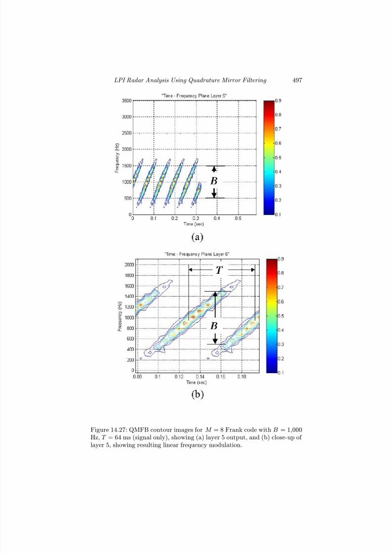
7/17/2019 1596932341 Intercept Radar.pdf
http://slidepdf.com/reader/full/1596932341-intercept-radarpdf 528/891
LPI Radar Analysis Using Quadrature Mirror Filtering 497
Figure 14.27: QMFB contour images for M = 8 Frank code with B = 1,000Hz, T = 64 ms (signal only), showing (a) layer 5 output, and (b) close-up of layer 5, showing resulting linear frequency modulation.
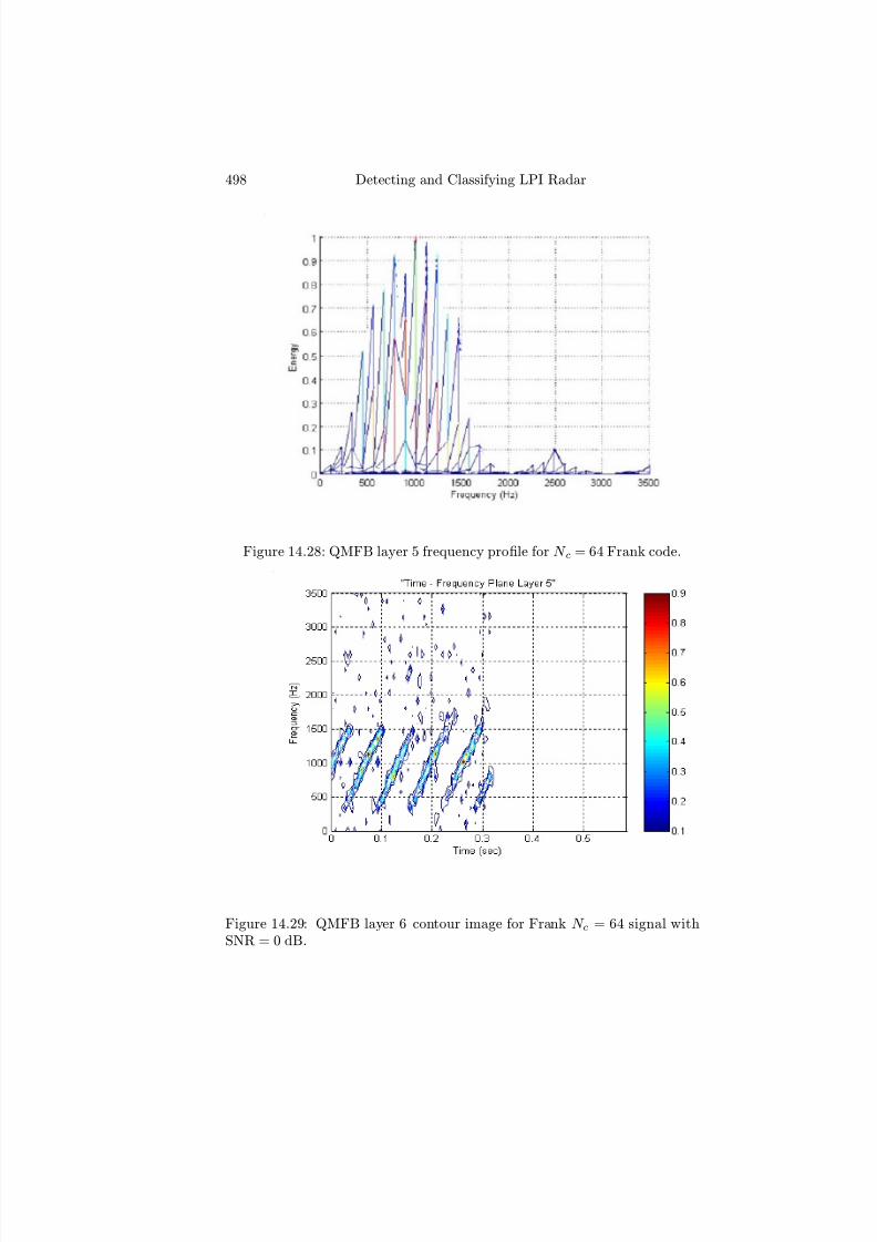
7/17/2019 1596932341 Intercept Radar.pdf
http://slidepdf.com/reader/full/1596932341-intercept-radarpdf 529/891
498 Detecting and Classifying LPI Radar
Figure 14.28: QMFB layer 5 frequency profile for N c = 64 Frank code.
Figure 14.29: QMFB layer 6 contour image for Frank N c = 64 signal withSNR = 0 dB.

7/17/2019 1596932341 Intercept Radar.pdf
http://slidepdf.com/reader/full/1596932341-intercept-radarpdf 530/891
LPI Radar Analysis Using Quadrature Mirror Filtering 499
quency modulation. Note that the resulting bandwidth is easily identified.The QMFB results for the T2(2) to T4(2) are shown in Appendix M.
14.11 Costas Frequency Hopping Analysis
In this section, five code periods of a Costas frequency hopping signal areexamined. The Costas code within each period is 4, 7, 1, 6, 5, 2, and 3 kHz.In Figure 14.32(a), the QMFB layer 4 shows that the frequencies can easilybe identified. The close-up in Figure 14.32(b) reveals that no modulation ispresent on the frequency. Figure 14.33 shows layer 6 with a finer frequencyresolution. Note the spread in time, demonstrating the trade-off in resolutionfrom one layer to the next.
14.12 FSK/PSK Signal Analysis
When a binary phase code modulation is added to the frequency hoppingsignal, the bandwidth about the carrier is increased. The QMFB layer 4results for the FH code above, with a binary 5-bit Barker code added, isshown in Figure 14.34. Note that in the close-up figure, the phase modulationis clearly present. In Figure 14.35, the QMFB layer 6 is shown. Due to thedecrease in time resolution, the phase modulation is not as distinct as inlayer 4.
14.13 Noise Waveform AnalysisThe random noise waveforms discussed in Chapter 7 can also be examinedwith the QMFB. In Figure 14.36, a random noise waveform that has a band-width of B = 300 MHz, carrier frequency of f c = 350 MHz and a code periodof T = 4 μs is examined with the QMFB layer 6 (out of 13). Note that thebandwidth can be easily identified as well as the carrier frequency and codeperiod. The random noise plus triangular FMCW waveform with tm = 1 μs,∆F = 300 MHz, B = 300 MHz, and f c = 350 MHz is shown in Figure 14.37.Note in layer 6 the noise bandwidth and the FMCW modulation are easilyidentified. The use of the QMFB to examine the random noise FMCW plussine waveform is left as an exercise for the reader.
The random binary phase modulation waveform is shown in Figure 14.38using layer 7. For this waveform, f
c = 300 MHz, cpp = 3, and
tb = 10 ns. With N c = 64 and 5 code periods included, T = 3.2 μs. Thesesignal parameters can be easily identified from layer 7. For the signal only,layer 2 is examined in Figure 14.39 and shows the direct correlation of thephase modulation parameters used.

7/17/2019 1596932341 Intercept Radar.pdf
http://slidepdf.com/reader/full/1596932341-intercept-radarpdf 531/891
500 Detecting and Classifying LPI Radar
Figure 14.30: QMFB contour images for polytime T1(2) code with resultingB = 1,750 Hz, T = 16 ms (signal only), showing (a) layer 2 output, and(b) close-up layer 2, showing detailed frequency changes due to phase codes.

7/17/2019 1596932341 Intercept Radar.pdf
http://slidepdf.com/reader/full/1596932341-intercept-radarpdf 532/891
LPI Radar Analysis Using Quadrature Mirror Filtering 501
Figure 14.31: QMFB contour images for polytime T1(2) code with resultingB = 1,750 Hz, T = 16 ms (signal only), showing (a) layer 4 output, and(b) close-up of layer 4 showing resulting linear frequency modulation.

7/17/2019 1596932341 Intercept Radar.pdf
http://slidepdf.com/reader/full/1596932341-intercept-radarpdf 533/891
502 Detecting and Classifying LPI Radar
Figure 14.32: QMFB contour images for layer 4 for FSK code using Costassequence, showing (a) layer 4 output, and (b) close-up of layer 4 showingfrequency resolution.

7/17/2019 1596932341 Intercept Radar.pdf
http://slidepdf.com/reader/full/1596932341-intercept-radarpdf 534/891
LPI Radar Analysis Using Quadrature Mirror Filtering 503
Figure 14.33: QMFB contour images for layer 6 for FSK code using Costassequence, showing (a) layer 6 output, and (b) close-up of layer 6 showingfrequency resolution.

7/17/2019 1596932341 Intercept Radar.pdf
http://slidepdf.com/reader/full/1596932341-intercept-radarpdf 535/891
504 Detecting and Classifying LPI Radar
Figure 14.34: QMFB contour images for layer 4 for FSK/PSK code usingCostas sequence plus 5-bit Barker code cpp = 5 (signal only), showing(a) layer 4 output, and (b) close-up of layer 4 showing Barker phase modula-tion.

7/17/2019 1596932341 Intercept Radar.pdf
http://slidepdf.com/reader/full/1596932341-intercept-radarpdf 536/891
LPI Radar Analysis Using Quadrature Mirror Filtering 505
Figure 14.35: QMFB contour images for layer 6 for FSK/PSK code usingCostas sequence plus 5-bit Barker code cpp = 5 (signal only), showing (a)layer 6 output, and (b) close-up layer 6 showing Barker phase modulation.

7/17/2019 1596932341 Intercept Radar.pdf
http://slidepdf.com/reader/full/1596932341-intercept-radarpdf 537/891
506 Detecting and Classifying LPI Radar
Figure 14.36: QMFB contour image for the random noise waveform showingthe extraction of the bandwidth and carrier frequency from l = 6.
14.14 Summary
The QMFB theory was presented in this chapter and several examples wereused to demonstrate the time-frequency results. To extract the unknownsignal parameters, several layers must be examined to determine those thatprovide the best information. The phase changes can be identified from thelower layers, while the frequency information is best obtained from the higherlayers.
Contrary to the Wigner-Ville distribution, and Choi-Williams distribu-tion, the QMFB performs remarkably well for the FSK Costas code andFSK/PSK (binary phase code) signal. Not only were the frequency hopsidentified, but the frequency duration could also be indentified, as well asthe binary phase modulation if present. For the FSK/PSK target signal re-ported, the QMFB was not able to identify any meaningful signal parametersfor the same reason that the PWVD could not. The use of the QMFB was
also demonstrated to work remarkably well with the random noise modula-tions. The main drawback is the fact that even if the most useful results arefrom, for example, layer 7, all of the other layers prior to layer 7 must still becomputed.
The presentation of the QMFB results to a trained operator will allow thesignal parameters to be extracted, and can enable good classification results

7/17/2019 1596932341 Intercept Radar.pdf
http://slidepdf.com/reader/full/1596932341-intercept-radarpdf 538/891
LPI Radar Analysis Using Quadrature Mirror Filtering 507
Figure 14.37: QMFB contour image for the random noise plus FMCW wave-form showing the extraction of the noise bandwidth, FMCW modulation, andcarrier frequency.
Figure 14.38: QMFB contour image layer 7 for the random binary phasemodulation showing the extraction of the bandwidth, and carrier frequency.

7/17/2019 1596932341 Intercept Radar.pdf
http://slidepdf.com/reader/full/1596932341-intercept-radarpdf 539/891
508 Detecting and Classifying LPI Radar
Figure 14.39: QMFB contour image layer 2 for random binary phase modu-lation showing the direct correlation of the phase modulation used to createone code period.

7/17/2019 1596932341 Intercept Radar.pdf
http://slidepdf.com/reader/full/1596932341-intercept-radarpdf 540/891
LPI Radar Analysis Using Quadrature Mirror Filtering 509
when the information from several layers is combined. The use of the QMFBin noisy environments, however, gives problems in parameter identification,and further image processing is necessary.
References
[1] Burrus, C. S., Gopinath R. A., and Guo, H., Introduction to Wavelets and
Wavelet Transforms, A Primer , Prentice Hall, Upper Saddle River, NJ, 1998.
[2] Chui, C. K., Wavelets: A Mathematical Tool for Signal Analysis, First Edi-
tion, SIAM, Philadelphi, PA, 1997.
[3] Vetterli, M., and Herley, C., “Wavelets and filter banks: Theory and design,”IEEE Trans. on Signal Processing , Vol. 40, No. 9, pp. 2207—2232, Sept.
1992.[4] Mitra, S., Digital Signal Processing, A Computer-Based Approach, Second
Edition , McGraw-Hill, Boston, MA, 2001.
[5] Al-Namiy, F., and Nigam, M. J., “On the design of 2-band FIR QMF filterbanks using WLS techniques,” Proc. of the Fourth IEEE International Con-
ference on High Performance Computing in the Asia-Paci fi c Region , Vol. 2,pp. 772—776, May 2000.
[6] Goh, C. K., and Lim, Y. C., “A WLS algorithm for the design of low-delayquadrature mirror filter banks,” Proceedings of the IEEE International Sym-
posium on Circuits and Systems , Vol. 1, pp. 615—618, May 2000.
[7] Zahhad, A., and M. A. Sabah, “Design of selective M-channel perfect recon-struction FIR filter banks,” IEE Electronics Letters, Vol. 35, No. 15, pp.1223—1225, 1999.
[8] Zhang, Z., and L. Jiao, “A simple method for designing pseudo QMF banks,”Proceedings of the IEEE International Conference on Communication Tech-
nology, Vol. 2, pp. 1538—1541, Aug. 2000.
[9] Farrell, T., and Prescott, G., “A Method for Finding Orthogonal WaveletFilters with Good Energy Tiling Characteristics,” IEEE Trans. on Signal
Processing , Vol. 47, No. 1, pp. 220—223, Jan. 1999.
[10] Farrell, T., and Prescott, G., “A Nine-Tile Algorithm for LPI Signal Detec-tion Using QMF Filter Bank Trees,” Proceedings of the IEEE Conference on
Military Communications MILCOM ’96 , Vol. 3, pp. 974—978, 1996.
[11] Proakis, J., and Manolakis, D., Digital Signal Processing. Principles, Algo-
rithms, and Applications, Third Edition , Prentice Hall, Upper Saddle River,NJ, 1996.
[12] Herley, C., et. al., “Tilings of the time-frequency plane: Construction of arbitrary orthogonal bases and fast tiling algorithms,” IEEE Transactions on
Signal Processing , Vol. 41, No. 12, pp. 3341—3359, Dec. 1993.
[13] Shang, Y., Longzhuang, L., and Ho, K. C., “Optimization design of filterbanks for wavelet denoising,” Proceedings of the 5th International Conference
on Signal Processing, Vol. 1, pp. 306—310, Aug. 2000.

7/17/2019 1596932341 Intercept Radar.pdf
http://slidepdf.com/reader/full/1596932341-intercept-radarpdf 541/891
510 Detecting and Classifying LPI Radar
[14] Chan, L. A., and Nasrabadi, N. M., “An application of wavelet-based vectorquantization in target recognition,” Proceedings of the IEEE International
Joint Symposium on Intelligence and Systems, pp. 274—281, Nov. 1996.
[15] Ho, K. C., Prokopiw W., and Chan, Y. T., “Modulation identification of digital signals by the wavelet transform,” IEE Proceedings Radar, Sonar and
Navigation, Vol. 147, No. 4, pp. 169—175, Aug. 2000.
[16] Farrell, T., and Prescott, G., “A Low Probability of Intercept Signal DetectionReceiver Using Quadrature Mirror Filter Bank Trees,” IEEE International
Conference on Acoustics, Speech and Signal Processing, Vol. 3, pp. 1558—1561, March 1996.
[17] Copeland, D. B., and Pace, P. E., “Detection and analysis of FMCW andP-4 polyphase LPI waveforms using quadrature mirror filter trees,” Proceed-
ings of the IEEE International Conference on Acoustics Speech and Signal
Processing , Vol. 1, May 2002.
[18] Taboada, F., et al., “Intercept receiver signal processing techniques to de-tect low probability of intercept radar signals,” Proceedings of the 5th Nordic
Signal Processing Symposium, Hurtigruta Tromso, Norway, Oct. 2002.
[19] Jarpa, P., “Quantifying the diff erences in low probability of intercept radarwaveforms using quadrature mirror filtering,” Naval Postgraduate SchoolMaster’s Thesis, Sept. 2002.
Problems
1. (a) Using the LPIT, generate the FMCW waveform (signal only, SNR =0 dB, and SNR =
−6 dB) with a carrier frequency of 2 kHz, tm =
5 ms, and ∆F = 500 Hz. (b) Process the signals with the QMFBalgorithm. (c) For each useful layer, diagram your estimates of all thesignal parameters for signal only, SNR = 0 dB and SNR = −6 dB.
2. (a) Using the LPIT, generate a P4 waveform (signal only, SNR =0 dB, and SNR = −6 dB) with a carrier frequency of 2 kHz, N c = 128,tb = 1 ms, and f s = 7,000 Hz. (b) Process the signals with the QMFBalgorithm. (c) For each useful layer, diagram your estimates of all thesignal parameters for signal only, SNR = 0 dB, and SNR = −6 dB.
3. (a) Using the LPIT, generate the default FMCW waveform and thedefault P4 waveform. Load both signals into MATLAB, and truncatesuch that they both have the same size (be sure to at least include 1 to 2
code periods of each signal). (b) Add the two signals together and saveas a new signal (e.g., fmcw p4.mat). (c) Using the QMFB processing,analyze the signal and extract the waveform parameters for each signalthat is evident. (d) Repeat (b) and (c) for SNR = 0 dB. (e) Repeat (b)and (c) for SNR = −6 dB.
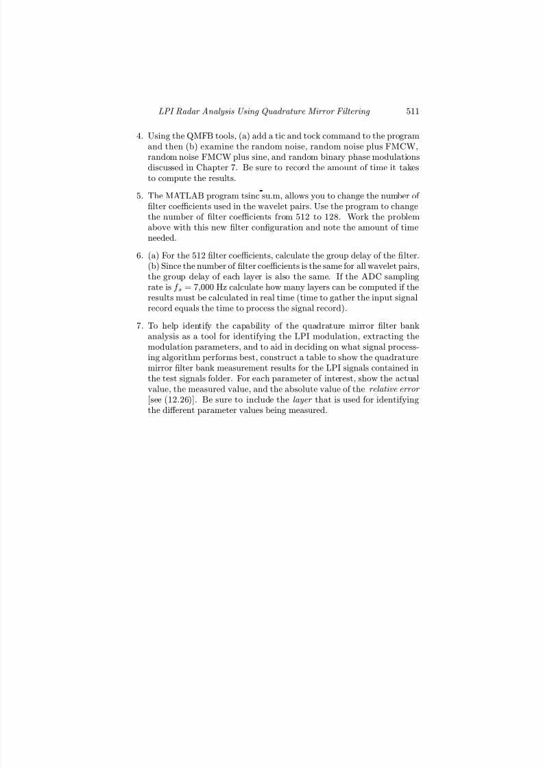
7/17/2019 1596932341 Intercept Radar.pdf
http://slidepdf.com/reader/full/1596932341-intercept-radarpdf 542/891
LPI Radar Analysis Using Quadrature Mirror Filtering 511
4. Using the QMFB tools, (a) add a tic and tock command to the programand then (b) examine the random noise, random noise plus FMCW,random noise FMCW plus sine, and random binary phase modulationsdiscussed in Chapter 7. Be sure to record the amount of time it takesto compute the results.
5. The MATLAB program tsinc su.m, allows you to change the number of filter coefficients used in the wavelet pairs. Use the program to changethe number of filter coefficients from 512 to 128. Work the problemabove with this new filter configuration and note the amount of timeneeded.
6. (a) For the 512 filter coefficients, calculate the group delay of the filter.
(b) Since the number of fi
lter coeffi
cients is the same for all wavelet pairs,the group delay of each layer is also the same. If the ADC samplingrate is f s = 7,000 Hz calculate how many layers can be computed if theresults must be calculated in real time (time to gather the input signalrecord equals the time to process the signal record).
7. To help identify the capability of the quadrature mirror filter bankanalysis as a tool for identifying the LPI modulation, extracting themodulation parameters, and to aid in deciding on what signal process-ing algorithm performs best, construct a table to show the quadraturemirror filter bank measurement results for the LPI signals contained inthe test signals folder. For each parameter of interest, show the actualvalue, the measured value, and the absolute value of the relative error
[see (12.26)]. Be sure to include the layer
that is used for identifyingthe diff erent parameter values being measured.

7/17/2019 1596932341 Intercept Radar.pdf
http://slidepdf.com/reader/full/1596932341-intercept-radarpdf 543/891

7/17/2019 1596932341 Intercept Radar.pdf
http://slidepdf.com/reader/full/1596932341-intercept-radarpdf 544/891
Chapter 15
Cyclostationary Spectral
Analysis for Detection of
LPI Radar Parameters
The Wigner-Ville distribution (Chapter 12), the Choi-Williams distribution(Chapter 13) and the quadrature mirror filter bank processing (Chapter 14)together give time-frequency results that allow the LPI parameters to be de-termined with good accuracy. This chapter presents an additional bifrequency
spectral analysis technique, known as cyclostationary processing, that off erssome additional capability in the detection and classification of LPI modu-lations. Instead of examining the LPI signals in the time-frequency domain,cyclostationary processing transforms the signal into the frequency-cycle fre-
quency domain. Two efficient methods for computing the cyclostationary
spectrum are presented: the time-smoothing FFT accumulation method, andthe direct frequency-smoothing method. The cyclostationary signal process-ing is then used to extract the parameters from the LPI radar waveformsdiscussed in Part I. The folder titled CYCLO contains the signal processingMATLAB files that allow the user to re-create any of the results presented,as well as new results of interest.
15.1 Introduction
Since the development of the theoretical concepts by Gardner in the early1980s, much work has been carried out to investigate the potential of cyclo-stationary spectral analysis for many signal processing tasks. Cyclostationary
processing has been investigated for use in the detection and identification of
513

7/17/2019 1596932341 Intercept Radar.pdf
http://slidepdf.com/reader/full/1596932341-intercept-radarpdf 545/891
514 Detecting and Classifying LPI Radar
weak spread-spectrum communication signals [1—3] and SATCOM signals [4].Cyclostationary signal models have also been used in array signal processingfor estimating the direction of arrival of multiple narrowband signals [5], aswell as building adaptive arrays [6, 7]. The estimation and detection of radarsignal parameters have been investigated [8—10]. In this chapter, a thoroughtreatment of this application is presented.
Cyclostationary spectral analysis is based on modeling the signal as acyclostationary process rather than a stationary process. A signal is cyclo-stationary of order n if and only if one can find some nth order nonlineartransformation of the signal that will generate finite-strength additive sinewave components that result in spectral lines [11]. For example, an n = 2or quadratic transformation (like the product of the signal with a delayedversion of itself, often used to detect BPSK signals) will generate spectrallines. That is, a signal x(t) is cyclostationary with cycle frequency α, if andonly if at least some of its delay product waveforms, z(t) = x(t − τ )x∗(t)
for some delays τ , exhibit a spectral line at frequency α, and if and only if the time fluctuations in at least some pairs of spectral bands of x(t), whosetwo center frequencies sum to α, are correlated. In contrast, for stationarysignals, only a spectral line at frequency zero can be generated. For signalswith periodic features (e.g., LPI radar signals), the advantage of using a cy-clostationary model is that nonzero correlation is exhibited between certainfrequency components when their frequency separation is related to the pe-riodicity of interest. Applications that use cyclostationary spectral analysisinclude time diff erence of arrival estimation, signal detection, identification,and parameter estimation. Many useful characteristics of LPI radar signalscan be determined, and are reflected in the cyclic autocorrelation function
and the spectral correlation density , which form the basis for cyclic spectralanalysis. These concepts are discussed below.
15.1.1 Cyclic Autocorrelation
To discuss the cyclic autocorrelation, we begin with the definition of thecorrelation integral. The correlation integral is defined as
Rc(x) =
∞
−∞
f (u)g(x + u)du (15.1)
Applying the FFT to both sides gives
F Rc(x) = F (s)G∗(s) (15.2)
If f (x) and g(x) are the same function, the integral above is called the auto-
correlation function and cross correlation if they diff er. The autocorrelation
function is a quadratic transformation of the signal, and may be interpretedas a measure of the predictability of the signal at time t + τ based on knowl-edge of the signal at time t. When considering a time series of length T , the
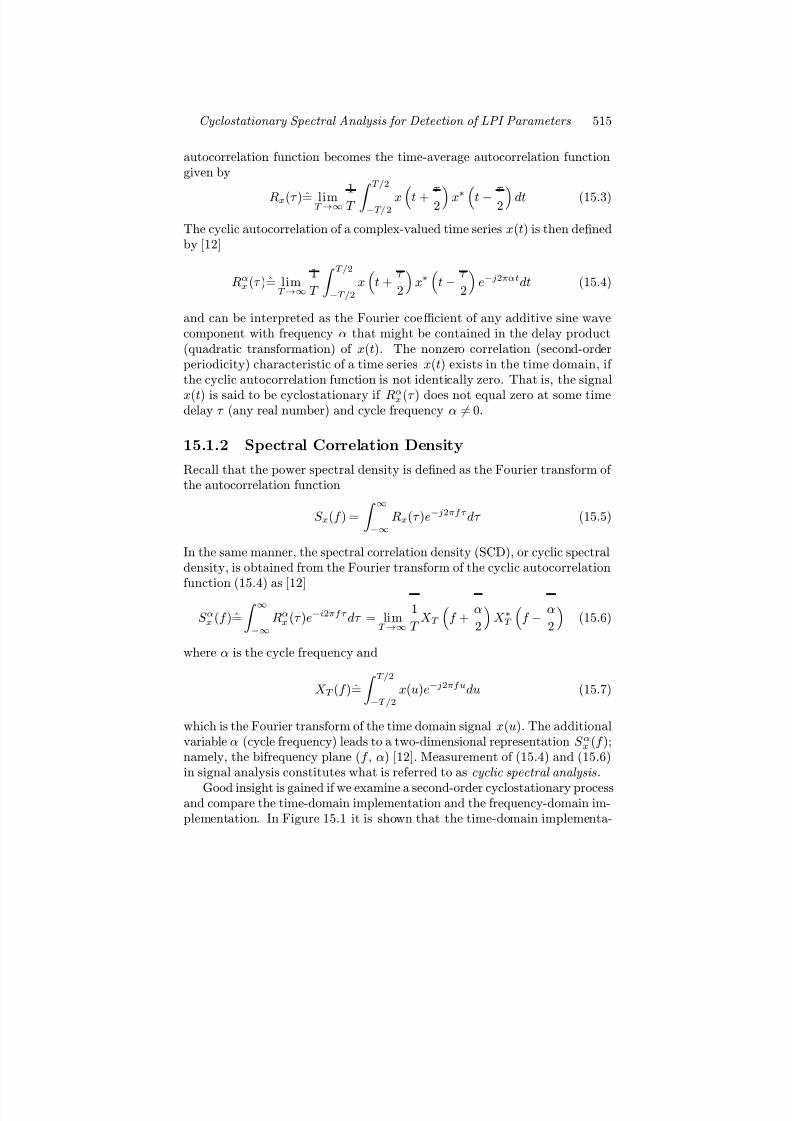
7/17/2019 1596932341 Intercept Radar.pdf
http://slidepdf.com/reader/full/1596932341-intercept-radarpdf 546/891
Cyclostationary Spectral Analysis for Detection of LPI Parameters 515
autocorrelation function becomes the time-average autocorrelation functiongiven by
Rx(τ )= limT →∞
1
T T/2−T/2
x
t + τ
2
x∗
t− τ
2
dt (15.3)
The cyclic autocorrelation of a complex-valued time series x(t) is then definedby [12]
Rα
x (τ )= limT →∞
1
T
T/2−T/2
x
t + τ
2
x∗
t− τ
2
e−j2παtdt (15.4)
and can be interpreted as the Fourier coefficient of any additive sine wavecomponent with frequency α that might be contained in the delay product(quadratic transformation) of x(t). The nonzero correlation (second-orderperiodicity) characteristic of a time series x(t) exists in the time domain, if the cyclic autocorrelation function is not identically zero. That is, the signal
x(t) is said to be cyclostationary if Rαx(τ ) does not equal zero at some time
delay τ (any real number) and cycle frequency α = 0.
15.1.2 Spectral Correlation Density
Recall that the power spectral density is defined as the Fourier transform of the autocorrelation function
S x(f ) =
∞
−∞
Rx(τ )e−j2πf τ dτ (15.5)
In the same manner, the spectral correlation density (SCD), or cyclic spectraldensity, is obtained from the Fourier transform of the cyclic autocorrelation
function (15.4) as [12]
S αx (f )=
∞
−∞
Rα
x (τ )e−i2πf τ dτ = limT →∞
1
T X T
f +
α
2
X ∗T
f −
α
2
(15.6)
where α is the cycle frequency and
X T (f )=
T/2−T/2
x(u)e−j2πfudu (15.7)
which is the Fourier transform of the time domain signal x(u). The additionalvariable α (cycle frequency) leads to a two-dimensional representation S αx (f );namely, the bifrequency plane (f , α) [12]. Measurement of (15.4) and (15.6)in signal analysis constitutes what is referred to as cyclic spectral analysis .
Good insight is gained if we examine a second-order cyclostationary processand compare the time-domain implementation and the frequency-domain im-plementation. In Figure 15.1 it is shown that the time-domain implementa-

7/17/2019 1596932341 Intercept Radar.pdf
http://slidepdf.com/reader/full/1596932341-intercept-radarpdf 547/891
516 Detecting and Classifying LPI Radar
Figure 15.1: Time-domain implementation of a second-order cyclostationaryprocess.
tion consists of a delay (τ i) and multiply operation followed by the multiplica-tion by the exponential cycle frequency term. The expected value then givesthe cyclic autocorrelation function Rα
x(τ ) and the subsequent FFT gives thespectral correlation density S αx (f ). With this perspective, it is easy to seethat if the signal x(t) contains a periodic component and the delay is chosenproperly, a strong sinusoid will be present at the output.
A frequency-domain implementation of a second-order cyclostationaryprocess is shown in Figure 15.2. The input signal x(t) with spectral represen-tation X (ν ), is split into two channels and multiplied by the two exponentialfactors that are a function of the cycle frequency and are complex conjugatesof each other. The time-domain output signals are u(t) and s(t) which havespectral representations of U (ν ) and S (ν ) respectively. This time-domainmultiplication results in a spectral shift of u(t) by −α/2 and a spectral shiftof s(t) by α/2. Figure 15.3 shows the spectral representations X (ν ), U (ν ),and S (ν ) and illustrates the narrowband spectral components of x(t) beingaligned at ν = f . Both u(t) and s(t) are filtered with a bandpass filter with
bandwidth B and center frequency f . Note that this captures the narrowbandspectral components of x(t) centered at f + α/2 and f − α/2. The Fouriertransform is taken of both filter outputs and then the correlation of the twospectrums is computed. The expected value of the correlation output is thenthe spectral correlation density function S αx (f ).
15.2 Spectral Correlation Density Estimation
Estimates of the cyclic spectral density or SCD can be obtained via time orfrequency-smoothing techniques. Since the signals being analyzed are definedover a finite time interval ∆t, the cyclic spectral density is only an estimate .An estimate of the SCD can be obtained by the time-smoothed cyclic peri-odogram given by
S αx (f ) ≈ S αxT W
(t, f )∆t = 1
∆t
t+(∆t/2)
t−(∆t/2)
S xT W
(u, f )du (15.8)

7/17/2019 1596932341 Intercept Radar.pdf
http://slidepdf.com/reader/full/1596932341-intercept-radarpdf 548/891
Cyclostationary Spectral Analysis for Detection of LPI Parameters 517
Figure 15.2: Frequency-domain implementation of a second-order cyclosta-
tionary process.
Figure 15.3: Frequency-domain representation of (a) x(t) [X (ν )], (b) modu-
lation of x(t) by −α/2 [U (ν )], and (c) modulation of x(t) by α/2 [S (ν )].
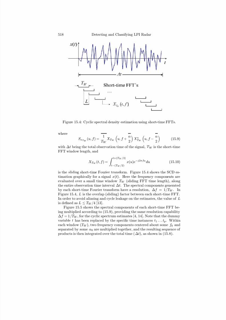
7/17/2019 1596932341 Intercept Radar.pdf
http://slidepdf.com/reader/full/1596932341-intercept-radarpdf 549/891
518 Detecting and Classifying LPI Radar
Figure 15.4: Cyclic spectral density estimation using short-time FFTs.
where
S xT W
(u, f ) = 1
T W X T W
u, f +
α
2
X ∗T W
u, f −
α
2
(15.9)
with ∆t being the total observation time of the signal, T W is the short-timeFFT window length, and
X T W (t, f ) =
t+(T W /2)
t−(T W /2)
x(u)e−j2πfudu (15.10)
is the sliding short-time Fourier transform. Figure 15.4 shows the SCD es-timation graphically for a signal x(t). Here the frequency components areevaluated over a small time window T W (sliding FFT time length), alongthe entire observation time interval ∆t. The spectral components generatedby each short-time Fourier transform have a resolution, ∆f = 1/T W . InFigure 15.4, L is the overlap (sliding) factor between each short-time FFT.In order to avoid aliasing and cycle leakage on the estimates, the value of Lis defined as L ≤ T W /4 [13].
Figure 15.5 shows the spectral components of each short-time FFT be-ing multiplied according to (15.9), providing the same resolution capability∆f = 1/T W , for the cyclic spectrum estimates [4, 14]. Note that the dummyvariable t has been replaced by the specific time instances t1 . . . t p. Within
each window (T W ), two frequency components centered about some f 0 andseparated by some α0 are multiplied together, and the resulting sequence of products is then integrated over the total time (∆t), as shown in (15.8).

7/17/2019 1596932341 Intercept Radar.pdf
http://slidepdf.com/reader/full/1596932341-intercept-radarpdf 550/891
Cyclostationary Spectral Analysis for Detection of LPI Parameters 519
Figure 15.5: Sequence of frequency products for each short-time Fourier trans-form.
The estimation S αx (f ) ≈ S αxT W
(t, f )∆t can be made as reliable and accu-
rate as desired for any given t and ∆f , and for all f by making ∆t sufficientlylarge, provided that (15.4) exists within the interval ∆t and that a substantialamount of smoothing is carried out over ∆t. This leads to the Grenander’s
uncertainty condition ∆t∆f 1 [14]. This uncertainty condition means thatthe observation time (∆t) must greatly exceed the time window (T W ) thatis used to compute the spectral components. A data taper window is also
used to minimize the eff ects of cycle and spectral leakage (estimation noise),introduced by frequency component side lobes [14]. The spectral componentsobtained from the short-time FFT have a resolution of
∆f = 1
T W (15.11)
The cycle frequency resolution of the estimate is related to the total observa-tion time by
∆α = 1
∆t (15.12)
The estimation of some (f 0, α0) represents a very small area on the bifre-quency plane, as shown in Figure 15.6, and, since one needs a significant
number of estimates to represent the cyclic spectrum adequately, it followsthat obtaining estimates becomes very computationally demanding, and effi-cient algorithms are required [15].

7/17/2019 1596932341 Intercept Radar.pdf
http://slidepdf.com/reader/full/1596932341-intercept-radarpdf 551/891
520 Detecting and Classifying LPI Radar
Figure 15.6: Frequency and cycle frequency resolutions on the bifrequencyplane (adapted from [3, 15]).
15.3 Discrete Time Cyclostationary
Algorithms
Cyclostationary signal processing can be used to extract the parameters fromthe sampled LPI signals in an intercept receiver, when moderate to largeamounts of additive noise are present. With the signal displayed on the bifre-quency plane (frequency-cycle frequency) the intercept receiver or operatorcan examine and compare the modulation characteristics, using several al-gorithms that estimate the SCD. Computationally efficient algorithms forimplementation of time- and frequency-smoothing techniques are discussedin [16]. These are the FFT accumulation method (FAM), a time-smoothingalgorithm, and the direct frequency-smoothing method (DFSM), a frequency-smoothing algorithm, as described below. The temporal and spectral smooth-ing equivalence is also addressed in [9].
15.3.1 The Time-Smoothing FFT Accumulation Method
The time-smoothing FFT accumulation method was developed to reduce thenumber of computations required to estimate the cyclic spectrum [3]. This
technique divides the bifrequency plane into smaller regions called channel pair regions, and computes the estimates one block at a time using the fastFourier transform. Describing the estimated time-smoothed periodogram

7/17/2019 1596932341 Intercept Radar.pdf
http://slidepdf.com/reader/full/1596932341-intercept-radarpdf 552/891
Cyclostationary Spectral Analysis for Detection of LPI Parameters 521
Figure 15.7: Block diagram of the FAM (adapted from [3, 11]).
from (15.8) and (15.9), in discrete terms, yields
S γ XN
(n, k) = 1
N
N −1n=0
1
N X N
n, k +
γ
2
X ∗N
n, k −
γ
2
(15.13)
where
X N (n, k) =N −1
n=0
w(n)x(n)e−(j2πkn)/N
(15.14)
is the discrete Fourier transform of x(n), w(n) is the data taper window (e.g.,Hamming window), and the discrete equivalents of f and α are k and γ ,respectively. A block diagram of the FFT accumulation method is shown inFigure 15.7.
The algorithm consists of three basic stages: computation of the complexdemodulates (divided into data tapering, sliding N point Fourier transform,and baseband frequency translation sections), computation of the productsequences, and smoothing of the product sequences. Table 15.1 shows therelationship between the variables in (15.8), (15.9), and (15.13). The parame-ter N represents the total number of discrete samples within the observationtime, and N represents the number of points within the discrete short-time(sliding) FFT. In the FAM algorithm, spectral components of a sequence,
x(n), are computed using (15.14). Two components are multiplied (15.13) toprovide a sample of a cyclic spectrum estimate representing the finite channelpair region on the bifrequency plane, as shown in Figure 15.8. There are N 2

7/17/2019 1596932341 Intercept Radar.pdf
http://slidepdf.com/reader/full/1596932341-intercept-radarpdf 553/891
522 Detecting and Classifying LPI Radar
Table 15.1: Comparison of the Estimated Time-Smoothed PeriodogramExpressed in Continuous and Discrete Time
Name Continuous Time Discrete Time
SCD S αXT W
(t, f )∆t S γXN
(n, k)N
Short FFT size T W N
Observation time ∆t N Time t nFrequency f kCycle frequency α γ
Grenander’s Uncertainty M = (∆f /∆α) 1 M = (N/N ) 1Condition
channel pair regions in the bifrequency plane. Note the 16 small channel pairregions corresponding to a value of M = 4 in Figure 15.8.
A sequence of samples for any particular area may be obtained by multi-plying the same two components of a series of consecutive short-time slidingFFTs along the entire length of the input sequence. After the channelizationperformed by an N -point FFT sliding over the data with an overlap of Lsamples, the outputs of the FFTs are shifted in frequency in order to obtainthe complex demodulate sequences (see Figure 15.7) [4]. Instead of comput-ing an average of the product of sequences between the complex demodulates,as in (15.8), they are Fourier-transformed with a P -point (second) FFT. Thecomputational efficiency of the algorithm is improved by a factor of L, sinceonly N/L samples are processed for each point estimate. With f s the sam-pling frequency, the cycle frequency resolution of the decimated algorithm isdefined as γ res = f s/N (compare to ∆α = 1/∆t), the frequency resolutionis kres = f s/N (compare to ∆f = 1/T W ), and the Grenander’s UncertaintyCondition is M = N/N 1 (compare to ∆t∆f 1).
Figure 15.9 reveals that the estimates toward the top and the bottom(shaded areas) of the channel pair region do not satisfy the Uncertainty Con-dition. In order to minimize the variability of these point estimates, we canretain only those cyclic spectrum components that are within γ = ±kres/2from the center of the channel pair region [15]. A solution to resolve theentire area of the channel pair region without leaving gaps is to apply a datataper window on the frequency axis (such as a Hamming window), to obtainbetter coverage.
15.3.2 Direct Frequency-Smoothing Method
Direct frequency-smoothing algorithms first compute the spectral componentsof the data, and then execute spectral-correlation operations directly on thespectral components. Generally, the direct frequency-smoothing method is

7/17/2019 1596932341 Intercept Radar.pdf
http://slidepdf.com/reader/full/1596932341-intercept-radarpdf 554/891
Cyclostationary Spectral Analysis for Detection of LPI Parameters 523
Figure 15.8: Channel pair regions within the bifrequency plane (Adaptedfrom [3, 15]).
Figure 15.9: Cycle frequency and frequency resolutions of the Grenander’sUncertainty Condition (adapted from [3, 15]).
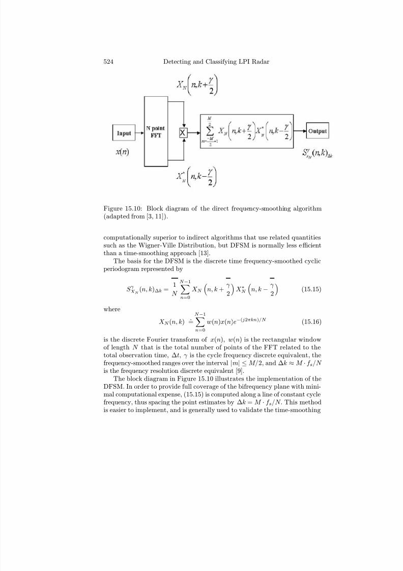
7/17/2019 1596932341 Intercept Radar.pdf
http://slidepdf.com/reader/full/1596932341-intercept-radarpdf 555/891
524 Detecting and Classifying LPI Radar
Figure 15.10: Block diagram of the direct frequency-smoothing algorithm(adapted from [3, 11]).
computationally superior to indirect algorithms that use related quantitiessuch as the Wigner-Ville Distribution, but DFSM is normally less efficientthan a time-smoothing approach [13].
The basis for the DFSM is the discrete time frequency-smoothed cyclicperiodogram represented by
S γ XN (n, k)∆k =
1
N
N −1
n=0
X N
n, k + γ
2
X ∗N
n, k −
γ
2
(15.15)
where
X N (n, k) =N −1n=0
w(n)x(n)e−(j2πkn)/N (15.16)
is the discrete Fourier transform of x(n), w(n) is the rectangular windowof length N that is the total number of points of the FFT related to thetotal observation time, ∆t, γ is the cycle frequency discrete equivalent, thefrequency-smoothed ranges over the interval |m| ≤ M/2, and ∆k ≈ M · f s/N is the frequency resolution discrete equivalent [9].
The block diagram in Figure 15.10 illustrates the implementation of theDFSM. In order to provide full coverage of the bifrequency plane with mini-mal computational expense, (15.15) is computed along a line of constant cycle
frequency, thus spacing the point estimates by ∆k = M · f s/N . This methodis easier to implement, and is generally used to validate the time-smoothing

7/17/2019 1596932341 Intercept Radar.pdf
http://slidepdf.com/reader/full/1596932341-intercept-radarpdf 556/891
Cyclostationary Spectral Analysis for Detection of LPI Parameters 525
approach, but may become more computationally demanding. This is espe-cially true in the last block in which the complex demodulate product se-quences are summed. Considerations on the parallel processing of both timeand frequency algorithms are discussed in [11]. Finally, we note that combi-nations of both time-smoothing and frequency-smoothing methods may alsobe advantageous for certain applications.
15.4 Test Signals
In order to grasp a good understanding of how the signals appear on thebifrequency plane, this section examines several test signals used in previ-ous chapters. The first test signal examined is a tone composed of a sin-gle carrier frequency with f c =1 kHz, and is sampled with sampling fre-quency f s = 7 kHz. The time-smoothing technique to estimate the SCDis demonstrated first using the real part of the input signal. Figure 15.11
shows the time-smoothing SCD results. Figure 15.11(a) shows the bifrequencyplane, and reveals that the signal’s frequency shows up at four separate loca-tions. The (γ , k) frequency pairs are (−2f c, 0), (0, f c), (0,−f c), and (2f c, 0).Figure 15.11(b) details a close-up of the time-smoothing estimation charac-teristics for the signal outlined in the box in Figure 15.11(a). For these resultsthe frequency resolution is ∆k = 128 Hz. With the Grenander’s uncertaintyvalue of M = 2, the cycle frequency ∆γ = 64 Hz. The overlap parameteris fixed at L = 4. The number of points in the first FFT N is the nextlargest power of 2 value of f s/∆k or N = 64. The number of points in thesecond FFT P is the next largest power of 2 value of 4 f s/∆N or P = 8. Thetotal number of signal samples integrated into the SCD are N = P L = 128.Note that in Figure 15.11(b), the γ = 2f c cycle frequency position lies at theresolved signal’s centroid.
The frequency-smoothing SCD results for the single-tone signal are shownin Figure 15.12. Figure 15.12(a) shows the bifrequency plane, andFigure 15.12(b) details a close-up of the frequency-smoothing estimation char-acteristics. The results serve to demonstrate the diff erences between the time-smoothing and frequency-smoothing techniques for estimating the SCD. Forthe frequency-smoothing results, ∆k = 128 Hz. The number of samples in-tegrated into the FFT is the next largest power of 2 value of f sM/∆f = 109or N = 128. Note in Figure 15.12(b), the γ = 2f c cycle frequency positiondoes not lie at the resolved signal’s centroid.
Next, the time-smoothing technique is used to estimate the SCD of atwo-tone signal (f c1 = 1 kHz and f c2 = 2 kHz). Figure 15.13 shows thetime-smoothing SCD results. Figure 15.13(a) shows the bifrequency plane,
and reveals that the two tones show up in the four separate quadrants, alongwith the cross terms. Figure 15.13(b) details a close-up of the time-smoothingestimation characteristics for the signal outlined in the box in Figure 15.13(a).
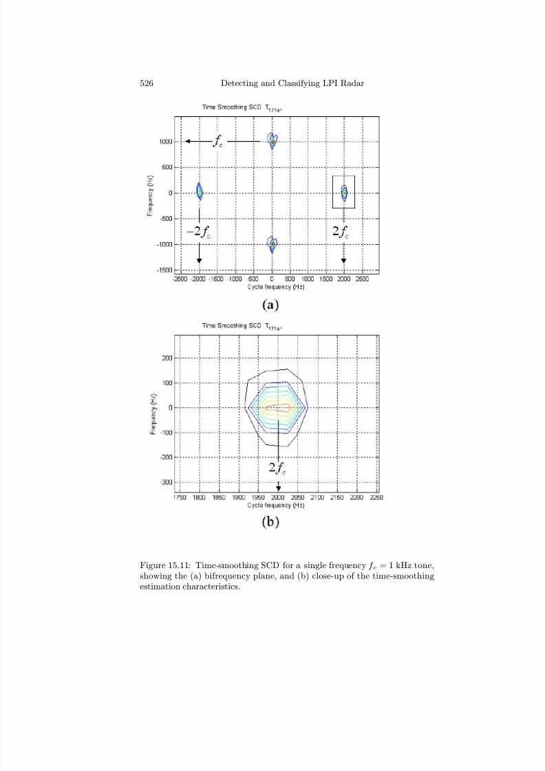
7/17/2019 1596932341 Intercept Radar.pdf
http://slidepdf.com/reader/full/1596932341-intercept-radarpdf 557/891
526 Detecting and Classifying LPI Radar
Figure 15.11: Time-smoothing SCD for a single frequency f c = 1 kHz tone,showing the (a) bifrequency plane, and (b) close-up of the time-smoothingestimation characteristics.
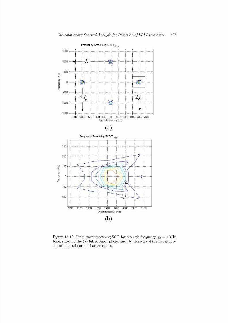
7/17/2019 1596932341 Intercept Radar.pdf
http://slidepdf.com/reader/full/1596932341-intercept-radarpdf 558/891
Cyclostationary Spectral Analysis for Detection of LPI Parameters 527
Figure 15.12: Frequency-smoothing SCD for a single frequency f c = 1 kHztone, showing the (a) bifrequency plane, and (b) close-up of the frequency-smoothing estimation characteristics.
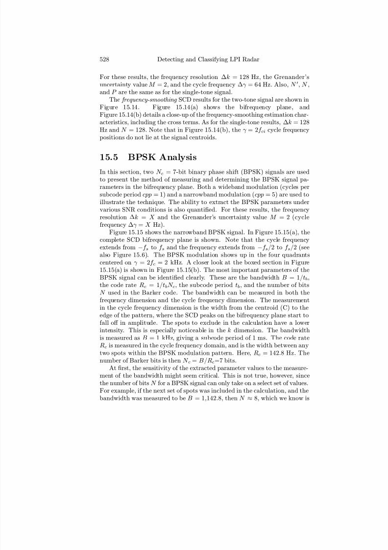
7/17/2019 1596932341 Intercept Radar.pdf
http://slidepdf.com/reader/full/1596932341-intercept-radarpdf 559/891
528 Detecting and Classifying LPI Radar
For these results, the frequency resolution ∆k = 128 Hz, the Grenander’suncertainty value M = 2, and the cycle frequency ∆γ = 64 Hz. Also, N , N ,and P are the same as for the single-tone signal.
The frequency-smoothing SCD results for the two-tone signal are shown inFigure 15.14. Figure 15.14(a) shows the bifrequency plane, andFigure 15.14(b) details a close-up of the frequency-smoothing estimation char-acteristics, including the cross terms. As for the single-tone results, ∆k = 128Hz and N = 128. Note that in Figure 15.14(b), the γ = 2f ci cycle frequencypositions do not lie at the signal centroids.
15.5 BPSK Analysis
In this section, two N c = 7-bit binary phase shift (BPSK) signals are usedto present the method of measuring and determining the BPSK signal pa-rameters in the bifrequency plane. Both a wideband modulation (cycles per
subcode period cpp = 1) and a narrowband modulation (cpp = 5) are used toillustrate the technique. The ability to extract the BPSK parameters undervarious SNR conditions is also quantified. For these results, the frequencyresolution ∆k = X and the Grenander’s uncertainty value M = 2 (cyclefrequency ∆γ = X Hz).
Figure 15.15 shows the narrowband BPSK signal. In Figure 15.15(a), thecomplete SCD bifrequency plane is shown. Note that the cycle frequencyextends from −f s to f s and the frequency extends from −f s/2 to f s/2 (seealso Figure 15.6). The BPSK modulation shows up in the four quadrantscentered on γ = 2f c = 2 kHz. A closer look at the boxed section in Figure15.15(a) is shown in Figure 15.15(b). The most important parameters of theBPSK signal can be identified clearly. These are the bandwidth B = 1/tb,the code rate Rc = 1/tbN c, the subcode period tb, and the number of bitsN used in the Barker code. The bandwidth can be measured in both thefrequency dimension and the cycle frequency dimension. The measurementin the cycle frequency dimension is the width from the centroid (C) to theedge of the pattern, where the SCD peaks on the bifrequency plane start tofall off in amplitude. The spots to exclude in the calculation have a lowerintensity. This is especially noticeable in the k dimension. The bandwidthis measured as B = 1 kHz, giving a subcode period of 1 ms. The code rateRc is measured in the cycle frequency domain, and is the width between anytwo spots within the BPSK modulation pattern. Here, Rc = 142.8 Hz. Thenumber of Barker bits is then N c = B/Rc=7 bits.
At first, the sensitivity of the extracted parameter values to the measure-ment of the bandwidth might seem critical. This is not true, however, since
the number of bits N for a BPSK signal can only take on a select set of values.For example, if the next set of spots was included in the calculation, and thebandwidth was measured to be B = 1,142.8, then N ≈ 8, which we know is

7/17/2019 1596932341 Intercept Radar.pdf
http://slidepdf.com/reader/full/1596932341-intercept-radarpdf 560/891
Cyclostationary Spectral Analysis for Detection of LPI Parameters 529
Figure 15.13: Time-smoothing SCD for a two-tone signal (f c1 = 1 kHz, f c2 =2 kHz), showing (a) the bifrequency plane, and (b) a close-up of the time-smoothing estimation characteristics.

7/17/2019 1596932341 Intercept Radar.pdf
http://slidepdf.com/reader/full/1596932341-intercept-radarpdf 561/891
530 Detecting and Classifying LPI Radar
Figure 15.14: Frequency-smoothing SCD for a two-tone signal (f c1 = 1 kHz,f c2 = 2 kHz) showing (a) the bifrequency plane, and (b) a close-up of thefrequency-smoothing estimation characteristics.

7/17/2019 1596932341 Intercept Radar.pdf
http://slidepdf.com/reader/full/1596932341-intercept-radarpdf 562/891
Cyclostationary Spectral Analysis for Detection of LPI Parameters 531
not correct. Therefore, too many spots were included in the measurement.Figure 15.16 shows a contour plot that illustrates the BPSK pattern and
measurement technique when the SNR = 0 dB. The white Gaussian noiseadded to the signal is distributed over a bandwidth equal to f s/2. The com-plete bifrequency plane is shown in Figure 15.16(a), and the boxed region isexamined closer in Figure 15.16(b). Note that the noise is suppressed sig-nificantly. This is due to the noise being uncorrelated. The centroid (C) isidentified, and the bandwidth is measured out to the row of spots just be-fore the crosshatch ends. The bandwidth in the frequency k dimension isalso shown. The bandwidth is measured as shown, and extends between thehighest and lowest corners of the crosshatch region. Note that since the noisehas enhanced the details of the crosshatch, the measurement is easier to takein the k dimension. The code rate is also easily measured between adjacentspots as shown in Figure 15.17.
The next signal examined is the narrowband 7-bit BPSK (cpp = 5). Since
the carrier frequency is f c = 1 kHz, the subcode period tb = 5 ms, resultingin a bandwidth of B = 200 Hz. The frequency-smoothing SCD is shown inFigure 15.18. Figure 15.19 illustrates the extraction of the narrowband BPSKsignal parameters when noise is present. The bandwidth B is measured inthe same manner as is the code rate Rc. This important example showsthat significant amounts of noise in the bifrequency plane can still give goodresults.
15.6 FMCW Analysis
In this section, a method is presented for extracting the parameters from atriangular FMCW radar signal. The signal shows up at four positions withinthe bifrequency plane, as illustrated in Figure 15.20 and Figure 15.21. Wefirst examine a ∆F = 250 Hz, f c = 1 kHz FMCW signal using frequency-smoothing. For these results, the frequency resolution ∆k = 16 Hz andthe Grenander’s uncertainty value M = 4 (cycle frequency ∆γ = 4 Hz). Thefrequency-smoothing SCD for one of the four positions is illustrated in Figure15.20, and is a unique pattern for the FMCW modulation. For this result,N = 1,024 and ∆k = 16 Hz.
The modulation centroid lies at a cycle frequency of γ = 2 kHz, indicatingthat the f c = 1 kHz. Note that the centroid lies to the right of the spot(as is the case for the frequency-smoothing SCD results). To determine themodulation bandwidth ∆F from the SCD, the width from the centroid outto the last large set of spots is measured on the cycle frequency axis. Notealso that ∆F can also be determined from the frequency axis by measuring
the total extent of the modulation as shown. The modulation period tm isdetermined by measuring Rc in the cycle frequency domain. In the SCD,Rc = 1/2tm for the FMCW signal. From Figure 15.20, Rc = 25 Hz, giving

7/17/2019 1596932341 Intercept Radar.pdf
http://slidepdf.com/reader/full/1596932341-intercept-radarpdf 563/891
532 Detecting and Classifying LPI Radar
Figure 15.15: Frequency-smoothing SCD patterns for an N c = 7-bit BPSKsignal, with f c = 1 kHz and cpp = 1, showing (a) the complete bifrequencyplane, and (b) a close-up illustrating the method of parameter measurements.
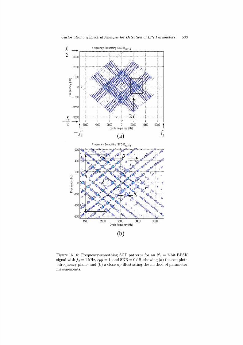
7/17/2019 1596932341 Intercept Radar.pdf
http://slidepdf.com/reader/full/1596932341-intercept-radarpdf 564/891
Cyclostationary Spectral Analysis for Detection of LPI Parameters 533
Figure 15.16: Frequency-smoothing SCD patterns for an N c = 7-bit BPSKsignal with f c = 1 kHz, cpp = 1, and SNR = 0 dB, showing (a) the completebifrequency plane, and (b) a close-up illustrating the method of parametermeasurements.

7/17/2019 1596932341 Intercept Radar.pdf
http://slidepdf.com/reader/full/1596932341-intercept-radarpdf 565/891
534 Detecting and Classifying LPI Radar
Figure 15.17: Frequency-smoothing SCD patterns for an N c = 7-bit BPSKsignal with f c = 1 kHz, cpp = 1, and SNR = −6 dB, showing (a) a partialbifrequency plane, and (b) a close-up illustrating the method of parametermeasurements.

7/17/2019 1596932341 Intercept Radar.pdf
http://slidepdf.com/reader/full/1596932341-intercept-radarpdf 566/891
Cyclostationary Spectral Analysis for Detection of LPI Parameters 535
Figure 15.18: Frequency-smoothing SCD patterns for an N c = 7-bit narrow-band BPSK signal with f c = 1 kHz and cpp = 5, showing the bifrequencyplane illustrating the method of parameter measurements.
tm = 20 ms.Figure 15.21 illustrates the extraction of the FMCW parameters when
noise is present. In Figure 15.21(a) the SNR = 0 dB. Note that the patternis still recognizable as being unique to the FMCW waveform. The noisepresent actually aids in identifying the centroid of the modulation. Themodulation bandwidth ∆F is measured in the same manner as shown inFigure 15.20 also with good fidelity. The measurement of Rc is also easilymade. In Figure 15.21(b) the SNR = −6 dB. With this level of noise, a sig-nificant degradation in the contour image results, and makes the modulationbandwidth difficult to measure in the cycle frequency dimension. However,the ∆F measurement can still be easily made, with only a slight bit of er-ror. Here ∆F = 240 Hz. The Rc value, however, can still be made with agood degree of accuracy. The extraction of the FMCW parameters from awideband signal ∆F = 500 is given in Appendix N.
15.7 Polyphase Code Analysis
In this section we look at the bifrequency plane results for the polyphasecodes, and demonstrate the bifrequency extraction techniques. We beginwith the Frank code example. The analysis of the wideband Frank signal

7/17/2019 1596932341 Intercept Radar.pdf
http://slidepdf.com/reader/full/1596932341-intercept-radarpdf 567/891
536 Detecting and Classifying LPI Radar
Figure 15.19: Frequency-smoothing SCD patterns for an N c = 7-bit narrow-band BPSK signal with f c = 1 kHz and cpp = 5, showing (a) the bifrequencyplane with SNR = 0 dB, and (b) SNR = −6 dB.

7/17/2019 1596932341 Intercept Radar.pdf
http://slidepdf.com/reader/full/1596932341-intercept-radarpdf 568/891
Cyclostationary Spectral Analysis for Detection of LPI Parameters 537
Figure 15.20: Frequency-smoothing SCD patterns for a ∆F = 250 Hz, tm =20-ms triangular FMCW signal with f c = 1 kHz.
with a long code period using the time-smoothing SCD is presented. For theseresults, the frequency resolution, ∆k = 16 Hz, and Grenander’s uncertaintyM = 4. With a longer code period T = 64 ms (N c = 64 subcodes, andcpp = 1), the Frank code signal converges to a more well-defined insect shape
on the bifrequency plane as shown in Figure 15.22(a). Interestingly enough,
all the longer phase codes derived from linear FM waveforms have this typeof shape, using the time-smoothing SCD technique. Figure 15.22(b) shows aclose-up of one of the four modulation patterns. Note the position of the head,abdomen, and wings that provide a convenient reference for measurementsof the signal parameters. Also note that the insect points to the right . Thedirection of the insect is important to help distinguish between the diff erentphase codes. The centroid (c) is symmetrically located within the patterncharacteristic of the time-smoothing SCD. The bandwidth can be measuredas the width from the centroid to the head, on the cycle frequency axis.A correlation can also be made using the bandwidth measurement on thefrequency axis and is the width between the wing tips.
Also indicated in Figure 15.22(b) is a box that is examined in closerdetail to illustrate the Rc measurement. Figures 15.23(a, b) illustrate the
measurement of Rc = 1/T . Figure 15.23(b) indicates Rc = 15.5 Hz, giv-ing a modulation period of 64 ms. Since the number of subcodes used byLPI radar are most often a power of 2 (e.g., 64 = 26), an accurate result
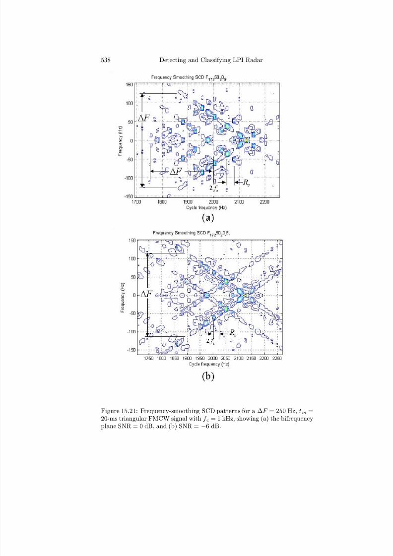
7/17/2019 1596932341 Intercept Radar.pdf
http://slidepdf.com/reader/full/1596932341-intercept-radarpdf 569/891
538 Detecting and Classifying LPI Radar
Figure 15.21: Frequency-smoothing SCD patterns for a ∆F = 250 Hz, tm =20-ms triangular FMCW signal with f c = 1 kHz, showing (a) the bifrequencyplane SNR = 0 dB, and (b) SNR = −6 dB.

7/17/2019 1596932341 Intercept Radar.pdf
http://slidepdf.com/reader/full/1596932341-intercept-radarpdf 570/891
Cyclostationary Spectral Analysis for Detection of LPI Parameters 539
Figure 15.22: Time-smoothing SCD insect patterns for the Frank code withN c = 64, f c = 1 kHz, and cpp = 1, with (a) the complete bifrequencyplane, and (b) a closer examination of one of the four modulation patternsillustrating the bandwidth measurements.

7/17/2019 1596932341 Intercept Radar.pdf
http://slidepdf.com/reader/full/1596932341-intercept-radarpdf 571/891
540 Detecting and Classifying LPI Radar
can be obtained, even from bifrequency planes with small SNR with N c =B/Rc = 64. Appendix O examines the Frank code with a shorter code pe-riod. The cyclostationary results for the P1, P2, P3, and P4 codes are given inAppendix P.
15.8 Polytime Code Analysis
In this section the frequency-smoothing SCD is used to examine the poly-time codes. We begin with the T1(2) code. The T1(2) code has an f c = 1kHz, and has a time-modulated binary phase shift (of various widths). Fig-ure 15.24(a) shows the bifrequency plane and the four modulation patterns.Figure 15.24(b) shows one of the four unique patterns, and illustrates howthe bandwidth of the signal can be measured. Recall that the bandwidthB is measuring the largest excursion in frequency, due to the shortest timephase code. For the case shown in Figure 15.24(b), B = 1,750 Hz, which
agrees with the results as measured by the time-frequency tools earlier. Notethat this value is not the modulation bandwidth ∆F of the linear FM signalused to derive the polytime phase modulation. Figure 15.25 shows a closerexamination of the bifrequency plane, and the measurement of Rc = 1/T =62.5 Hz. This gives the estimate for the code period as T = 16 ms. Notealso that an SCD spot exists at (γ = 2f c, k = 0). The results for the T2(2),T3(2), and T4(2) codes are given in Appendix Q.
15.9 Costas Frequency Hopping Results
In this section the time-smoothing SCD is used to determine what SCD prop-erties a Costas frequency hopping signal takes on. The time-smoothing SCD
was created using ∆γ = 16 and N = 2,048. The Costas sequence in thisexample is S = 4, 7, 1, 6, 5, 2, 3 and is used since this sequence is discussedin Chapter 6. The sampling frequency of the ADC is 15 kHz, and each Costasfrequency is generated with 20 cycles per frequency. That is, the time spentat each frequency is not a constant. Figure 15.26(a) shows the complete bifre-quency results. One of the four quadrants is shown in Figure 15.26(b). Thefrequencies within the sequence f ci show up at 2f ci and are outlined alongthe k = 0 axis. Also note the presence of the cross terms k = |f ci − f cj |/2.Although the SCD analysis does not let us determine the time sequence of information, we can, however, see that frequencies γ = 6 kHz and γ = 5 kHzare fired next to each other, as is the case for frequencies γ = 2 kHz andγ = 3 kHz, but we cannot determine the order.

7/17/2019 1596932341 Intercept Radar.pdf
http://slidepdf.com/reader/full/1596932341-intercept-radarpdf 572/891
Cyclostationary Spectral Analysis for Detection of LPI Parameters 541
Figure 15.23: Close examination of the time-smoothing SCD for the Frankcode with N c = 64, f c = 1 kHz, and cpp = 1, with (a) modulation cycles and(b) the measurement of Rc.
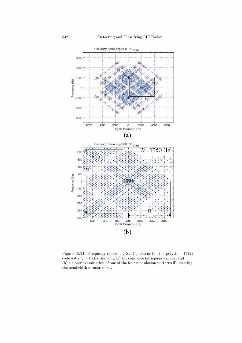
7/17/2019 1596932341 Intercept Radar.pdf
http://slidepdf.com/reader/full/1596932341-intercept-radarpdf 573/891
542 Detecting and Classifying LPI Radar
Figure 15.24: Frequency-smoothing SCD patterns for the polytime T1(2)code with f c = 1 kHz, showing (a) the complete bifrequency plane, and(b) a closer examination of one of the four modulation patterns illustratingthe bandwidth measurement.

7/17/2019 1596932341 Intercept Radar.pdf
http://slidepdf.com/reader/full/1596932341-intercept-radarpdf 574/891
Cyclostationary Spectral Analysis for Detection of LPI Parameters 543
Figure 15.25: Close examination of the frequency-smoothing SCD pattern forthe polytime T1(2) code illustrating the Rc measurement.
15.10 Random Noise Analysis
In the first example, a random noise waveform with a bandwidth of B = 300 MHz and carrier frequency of f c = 350 MHz was examined withthe time-smoothing SCD. Figure 15.27 shows that the bandwidth and carrier
frequency can easily be identified as expected.In the second example, a random noise plus FMCW waveform is exam-
ined. The FMCW waveform parameters used to modulate the noise are∆F = 300 MHz (from 200 to 500 MHz) and the carrier frequency isf c = 350 MHz. The noise bandwidth being modulated is B = 300 MHz.Since in this case the noise bandwidth and the modulation bandwidth over-lap, the total noise FMCW bandwidth transmitted is B = 300 MHz. Thetime-smoothing technique was chosen to estimate the SCD.
From Figure 15.28, the diamond is centered at 1,200 MHz, which is twicethe center frequency of the modulated signal. It might be expected that thecenter frequency would appear at 1,400 MHz, or twice the center frequencyof the two modulated signals (350 MHz for the noise and 350 MHz for theFMCW signal). The diff erence of 200 MHz is observed as an off set. Severalnoise plus FMCW waveforms were examined with diff erent modulation band-widths as summarized in Table 15.2. The relationship of the observed center
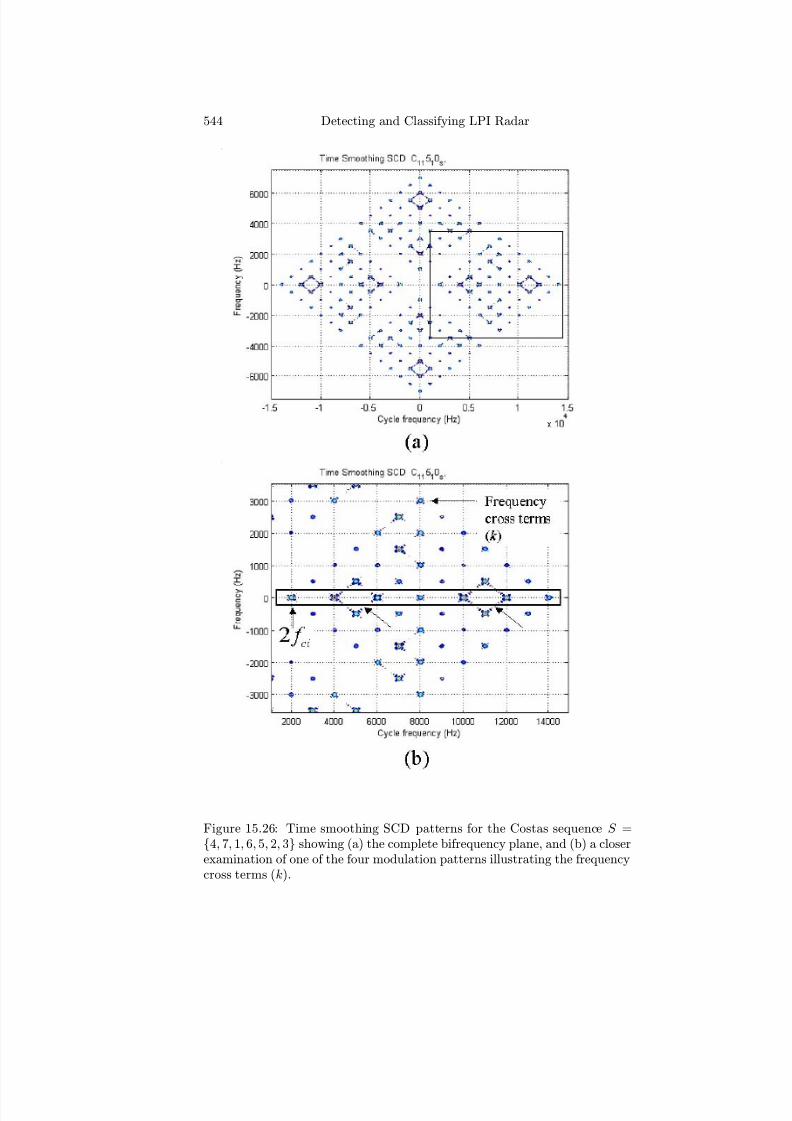
7/17/2019 1596932341 Intercept Radar.pdf
http://slidepdf.com/reader/full/1596932341-intercept-radarpdf 575/891
544 Detecting and Classifying LPI Radar
Figure 15.26: Time smoothing SCD patterns for the Costas sequence S =4, 7, 1, 6, 5, 2, 3 showing (a) the complete bifrequency plane, and (b) a closerexamination of one of the four modulation patterns illustrating the frequencycross terms (k).

7/17/2019 1596932341 Intercept Radar.pdf
http://slidepdf.com/reader/full/1596932341-intercept-radarpdf 576/891
Cyclostationary Spectral Analysis for Detection of LPI Parameters 545
Figure 15.27: Time smoothing SCD for the random noise waveform showingthe carrier frequency and the bandwidth measurements.
frequency off set as a function of the FMCW modulation bandwidth is left asan exercise for the reader. Other signal characteristics, such as the signalbandwidth of 300 MHz, can be measured along the cycle frequency axis, asexpected. The bandwidth can also be measured along the frequency axis aswell. This sweep bandwidth shows nicely in the QMFB results.
15.11 Summary
The cyclostationary signal processing was presented in this chapter, andseveral examples were used to demonstrate the bifrequency results. To ex-tract the unknown signal parameters, the bifrequency plane (frequency-cyclefrequency) is examined to determine directly (and indirectly) parameterssuch as the carrier frequency, code rate, bandwidth, and modulation pe-riod. Information not available includes any parameters that change as afunction of time (such as the signal’s phase). These phase changes, however,can be identified from the other signal processing tools that are included(such as the PWVD, CHOI, and QMFB). Measurement of the LPI signal
parameters agree well with the actual values. With moderate amounts of noise added, however, the measurement ability using the bifrequency analy-sis, does not degrade significantly but remains fairly robust since symmetrical

7/17/2019 1596932341 Intercept Radar.pdf
http://slidepdf.com/reader/full/1596932341-intercept-radarpdf 577/891
546 Detecting and Classifying LPI Radar
Figure 15.28: Time smoothing SCD for the random noise plus FMCW wave-form showing the bandwidth measurement and the carrier frequency off setthat appears in the bifrequency domain.
Table 15.2: Summary of Time Smoothing SCD for the Random Noise PlusFMCW Waveform Showing the Bandwidth Measurement and the CarrierFrequency Off set That Appears in the Bifrequency Domain
∆F (MHz) Off set (MHz) Center Frequency Observed500 250 1,150300 200 1,200200 100 1,300100 50 1,350
1 0 1,400

7/17/2019 1596932341 Intercept Radar.pdf
http://slidepdf.com/reader/full/1596932341-intercept-radarpdf 578/891
Cyclostationary Spectral Analysis for Detection of LPI Parameters 547
white Gaussian noise is not correlated and is suppressed in this spectral cor-relation technique.
The cyclostationary processing, however, does not perform well with theFSK Costas code and FSK/PSK (binary phase code) signal. This is mainlydue to a lack of temporal information needed, in order to identify the codesequence in time. The presentation of the cyclostationary results to a trainedoperator will allow the signal parameters to be extracted, and can enablegood classification results for the signals that are appropriate. The use of thecyclostationary processing in noisy environments is particularly good.
References
[1] Spooner, C. M., and Gardner, W. A., “Robust feature detection of signalinterception,” IEEE Trans. on Communications, Vol. 42, No. 5, pp. 2165—2173, May 1994.
[2] Gardner, W. A., “Signal interception: A unifying theoretical framework forfeature detection,” IEEE Trans. on Communications , Vol. 36, No. 8, pp.897—906, Aug. 1988.
[3] Gardner, W. A., and Spooner, C. M., “Signal interception: Performanceadvantages of cyclic feature detectors,” IEEE Trans. on Communications ,Vol. 40, No. 1, pp. 149—159, Jan. 1992.
[4] Tom, C., “Cyclostationary spectral analysis of typical SATCOM signals usingthe FFT accumulation method,” Defence Research Establishment Report No.
1280, Ottawa, Canada, Dec. 1995.
[5] Xin, J., and Sano, A., “Linear prediction approach to direction estimation of cyclostationary signals in multipath environment,” IEEE Trans. on Signal
Processing, Vol. 49, No. 4, pp. 710—720, April 2001.
[6] Yu, S-J., and Ueng, F-B., “Implementation of cyclostationary signal-basedadaptive arrays,” Elsevier Signal Processing , Vol. 80, pp. 2249—2254, 2000.
[7] Lee, J-H., and Lee, Y-T., “A novel direction-finding method for cyclostation-ary signals,” Elsevier Signal Processing , Vol. 81 pp. 1317—1323, 2001.
[8] Gini, F., Montanari, M., and Verrazzani, L., “Estimation of chirp radarsignals in compound-Gaussian clutter: A cyclostationary approach,” IEEE
Trans. on Signal Processing, Vol. 48, No. 4 pp. 1029—1039, April 2000.
[9] Skinner, B. J., Ingels, F. M., and Donohoe, J. P., “The eff ect of radar signalconstruction on detectability,” Proc. of the 26th Southeastern Symposium on
System Theory, pp. 147—150, March 1994.
[10] Gillman, A. M., “Non-cooperative detection of LPI/LPD signals via cyclicspectral analysis,” Air Force Institute of Technology, Master’s thesis, March1999.
[11] Gardner, W. A., Statistical Spectral Analysis: A Nonprobabilistic Theory ,Prentice-Hall, Englewood Cliff s, NJ, 1987.

7/17/2019 1596932341 Intercept Radar.pdf
http://slidepdf.com/reader/full/1596932341-intercept-radarpdf 579/891
548 Detecting and Classifying LPI Radar
[12] Gardner, W. A., “Exploitation of spectral redundancy in cyclostationary sig-nals,” IEEE Signal Processing Magazine , pp. 14—36, April 1991.
[13] Lima, A. F., Jr., “Analysis of low probability of intercept radar signals usingcyclostationary processing,” Naval Postgraduate School Master’s thesis, Sept.2002.
[14] Roberts, R. S., Brown, W. A., and Loomis, H. H., Jr., “A review of digitalspectral correlation analysis: Theory and implementation,” Cyclostationarity
in Communications and Signal Processing, IEEE Press, 1994.
[15] Roberts, R. S., Brown, W. A., and Loomis, H. H., Jr., “Computationally ef-ficient algorithms for cyclic spectral analysis,” IEEE Signal Processing Mag-
azine , pp. 38—49, April 1991.
[16] Brown, W. A., III, and Loomis H. H., Jr., “Digital implementations of spectralcorrelation analyzers,” IEEE Trans. on Signal Processing , Vol. 41, No. 2,pp. 703—720, Feb. 1993.
Problems
1. (a) Using the LPIT, generate the FMCW waveform (signal only, SNR =0 dB, and SNR = −6 dB) with a carrier frequency of 2 kHz,tm = 5 ms, and ∆F = 500 Hz. (b) Process the signals with boththe time-smoothing and frequency-smoothing algorithm. (c) For eachuseful algorithm, diagram your estimates of all the signal parametersfor signal only, SNR = 0 dB, and SNR = −6 dB.
2. (a) Using the LPIT, generate a P4 waveform (signal only,SNR = 0 dB, and SNR = −6 dB) with a carrier frequency of 2 kHz,N c = 128, tb = 1 ms, and f s = 7,000 Hz. (b) Process the signals withboth the time-smoothing and frequency-smoothing algorithm. (c) Foreach useful algorithm, diagram your estimates of all the signal parame-ters for signal only, SNR = 0 dB, and SNR = −6 dB.
3. (a) Using the LPIT, generate the default FMCW waveform and thedefault P4 waveform. Load both signals into MATLAB, and truncatesuch that they both have the same size (be sure to at least include 1to 2 code periods of each signal). (b) Add the two signals togetherand save as a new signal (e.g., fmcw p4.mat). (c) For each signal,use the cyclostationary processing to analyze and extract the waveformparameters that are evident. (d) Repeat (b) and (c) for SNR = 0 dB.(e) Repeat (b) and (c) for SNR = −6 dB.

7/17/2019 1596932341 Intercept Radar.pdf
http://slidepdf.com/reader/full/1596932341-intercept-radarpdf 580/891
Cyclostationary Spectral Analysis for Detection of LPI Parameters 549
4. To help identify the capability of the cyclostationary signal processingas a tool for identifying the LPI modulation, extracting the modulationparameters, and to aid in deciding on what signal processing algorithmperforms best, construct a table to show the bifrequency measurementresults for the LPI signals contained in the test signals folder. For eachparameter of interest, show the actual value, the measured value, andthe absolute value of the relative error [see (12.26)]. Be sure to includewhich frequency axis (frequency, cycle frequency) is used for identifyingthe diff erent parameter values being measured.

7/17/2019 1596932341 Intercept Radar.pdf
http://slidepdf.com/reader/full/1596932341-intercept-radarpdf 581/891

7/17/2019 1596932341 Intercept Radar.pdf
http://slidepdf.com/reader/full/1596932341-intercept-radarpdf 582/891
Chapter 16
Antiradiation Missiles
A Wild Weasel provides a Warsaw Pact SAM operator the maximum
opportunity to give his life for his country — “Relic quote of the Wild Weasel”
This chapter gives a brief account of the concept of suppression of enemyair defenses. The beginnings of SEAD and the development of antiradiationmissiles (ARMs) are presented. The use of ARMs in Vietnam and post-Vietnam is also presented. The design of ARM seekers is addressed and
the concept of dual-mode ARMs is discussed including ARM performancemetrics. The important ARMs from around the world are then reviewed andtheir performance given. Anti-ARM techniques that can be employed otherthan the use of LPI emitters are also presented.
16.1 Suppression of Enemy Air Defense
Suppression of enemy air defense (SEAD) is defined by the U.S. Depart-ment of Defense as “that activity that neutralizes, destroys or temporarilydegrades surface-based enemy air defenses by destructive and/or disruptivemeans” [1]. SEAD includes the use of air-to-ground missiles against an en-emy’s integrated air defense system (IADS). An IADS is an integration of air-
and ground-based sensors and the communication that links them together
551
7/17/2019 1596932341 Intercept Radar.pdf
http://slidepdf.com/reader/full/1596932341-intercept-radarpdf 583/891
552 Detecting and Classifying LPI Radar
with the weapons and command and control. SEAD capabilities fall withinthe traditional discipline of electronic warfare (EW), which includes electronicattack (EA), electronic protection (EP), and electronic warfare support (ES).SEAD is also an interdisciplinary construct that integrates EW as an activityof information operations with the use of EA capabilities such as antiradiation
missiles (ARMs) against the enemy’s IADS in an eff ort to obtain informationsuperiority. In suppression, the ARMs are fired and home in on the enemy’ssurface-based radar systems that are used to target their surface-to-air mis-siles (SAMs) against any incoming strike aircraft. In modern network-enabledwarfare, there is a dedicated aircraft assigned that specializes in the hard-killof enemy guidance radars by deploying ARMs [2]. The ARM relies on pas-sive detection of the radiation emitted from the radar. The ARM mission orsortie is an aircraft strike capability against radar directed/radar controlledmissile and gun system sites–the greatest threat to eff ective air operations.ARMs can also be fired preemptively in order to prevent the SAM radar from
coming up. The use of ARMs contributes to information superiority by pre-venting and reducing the enemys use of the electromagnetic spectrum whileprotecting our own spectrum vulnerabilities. That is, SEAD actions increasean air force’s ability to conduct air operations by reducing their vulnerabilityto air defense missiles and guns.
Below, the U.S. Army’s description of the various forms of SEAD are givenhighlighting their potential use in suppression of an enemy’s IADS [3].
• Campaign SEAD: SEAD operations that are preplanned, theaterwideeff orts conducted concurrently over an extended period against air de-fense systems normally located well behind enemy lines.
• Complementary SEAD: Those operations that involve continuously seek-ing enemy air defense system targets to destroy them.
• Localized SEAD: Those operations that support tactical air operations,Army aviation operations, reconnaissance, and the establishment of cor-ridors for ingress and egress routing for air force and army assets.
• Joint SEAD: Broad term that includes all suppression of enemy air de-fense activities provided by one component of the joint force in supportof another.
• Nonlethal SEAD: Aims to neutralize or degrade enemy IADS ratherthan destroy them. While nonlethal SEAD is most commonly associ-ated with the electronic jamming of IADS sensors and command, controland communications (C3) links, this is not the only form of nonlethalSEAD. Other forms of nonlethal SEAD include the use of specializedtactics to exploit known air defense system limitations and the use of stealth technology, or false targets, to deceive enemy air defenses. Note

7/17/2019 1596932341 Intercept Radar.pdf
http://slidepdf.com/reader/full/1596932341-intercept-radarpdf 584/891
Antiradiation Missiles 553
that: the threat of destruction alone may degrade an air defense sys-tems eff ectiveness by forcing its operators to employ defensive measuresthat would result in suboptimal system performance.
• Lethal SEAD: Measures taken to physically destroy one or more com-ponents of an IADS. Most hard-kill SEAD options involve specializedweapons such as ARMs, precision guided munitions (PGMs), and stand-off weapons (SOWs); the successful use of which will damage the enemysIADS and possibly inflict casualties among their crews. Lethal SEADcan suppress enemy air defenses for a potentially longer period thancan nonlethal measures. However, the success of lethal SEAD missionsdepends on adequate EW support to provide both accurate targetingand protection of the SEAD platform.
• Preemptive SEAD: This concept diff ers from lethal-SEAD practicesby preemptively disrupting enemy air defenses before they can engage
friendly aircraft. This is typically done by firing an ARM in the airin the direction of a SAM that is suspected to exist but which has notturned on its radar in the aim of preventing the SAM radar from comingup. Although an eff ective and necessary tactic, it is not efficient.
16.1.1 The Beginning of SEAD
Since the introduction of radar in World War II (WWII), radar was usedby both sides to alert ground-based air defenses and fighters of an impend-ing raid. The SEAD role originated in WWII when the German Luftwaff ebombed elements of the British CHAIN HOME early warning radar net dur-ing the Battle of Britain. This first SEAD attempt heralded a series of Allied SEAD developments made in response to the very eff ective German
radar-based air defenses encountered during the Allied bombing off ensive of Germany [4].
One of the first SEAD measures employed by the Allies was to drop chaff ,consisting of small strips of metal foil, from lead bombers or pathfinder air-craft to disrupt the German radar picture by creating thousands of falsetargets. If the location of the radars were discovered, they could be attacked,generally by bombing from a large formation. The British developed a radarhoming device (dubbed “Abdullah”) that would locate the enemy radar. Theaircraft that were equipped with the Abdullah were not armed and flew onlywith escort fighters. In addition, Ferret aircraft were used to detect the op-erating frequencies of German radars and radios so they could be jammed byEA equipment or physically attacked by the Ferret or other aircraft. SimilarSEAD measures were used in the Pacific theater during WWII and again
during the Korean conflict [4].

7/17/2019 1596932341 Intercept Radar.pdf
http://slidepdf.com/reader/full/1596932341-intercept-radarpdf 585/891
554 Detecting and Classifying LPI Radar
Figure 16.1: The Corvus antiradiation missile.
Figure 16.2: The Corvus antiradiation missile being loaded.
16.1.2 Early ARM Developments
In 1955, the U.S. Navy had a requirement for a long-range nuclear-armedheavy standoff air-to-surface missile to be employed by carrier-based attackbombers. In April 1955, the ASM-N-8 Raven project was initiated to developsuch a missile [5]. In the same year, a parallel project for an anti-radarmissile was redefined to cover the Raven requirements, and therefore theRaven project was canceled and the ASM-N-8 designation transferred to theCorvus . A development contract for the ASM-N-8 Corvus shown in Figure16.1 was awarded to Temco in January 1957, and the first flight test of an
XASM-N-8 prototype occurred in July 1959. Figure 16.2 shows the Corvusmissile being loaded with a special purpose cart. The Corvus was designed
7/17/2019 1596932341 Intercept Radar.pdf
http://slidepdf.com/reader/full/1596932341-intercept-radarpdf 586/891
Antiradiation Missiles 555
as an ARM, and had a passive radar seeker to home in on the emission of enemy radars at a speed of Mach 0.8 [6]. The Corvus seeker could also homeon nonradiating targets when they were illuminated by a compatible radar inthe launching aircraft. In this mode there was also a data-link between themissile and the launching aircraft, which could provide mid-course commandguidance until the missile’s seeker could detect the radar reflections from thetarget [7]. The missile could be launched from high or low altitudes, andmaximum ranges for high-altitude (15 km) launches were 315 km in ARMmode and 185 km in semiactive homing mode. Corvus was to be armed witha light-weight W-40 nuclear fission warhead (10 kT yield) [5].
By March 1960, the XASM-N-8 test program had progressed to fullyguided flights, but in July that year the Corvus program was terminated. Thereason was that overall responsibility for long-range nuclear air-to-surface mis-siles had been transferred to the U.S. Air Force, which regarded the Corvusas unnecessary [6].
16.1.3 Vietnam
The greatest SEAD advances were made during the Vietnam War in 1965when the eff ectiveness of the North Vietnamese IADS caused significantlosses. The initial U.S. response of launching conventional air strikes againstthe SAM sites resulted in heavy friendly losses [8]. The Soviet SA-2 SAMskilled at least 83 aircraft and forced the USAF to increase its SEAD capa-bility by building the F-100 Super Sabre Wild Weasel (an evolution of theFerret aircraft) in 90 days pairing experienced fighter pilots with electronicwarfare officers from the Strategic Air Command. The F-100 was followed bythe F-105G Wild Weasel and the F-4G Wild Weasel [9].
The Wild Weasels were free-roving hunters that baited SAM sites at point
blank range. The Wild Weasel mission was developed by the U.S. Air Forcein 1965, during the Vietnam War era. Its primary concept was the use of two-seat aircraft, to counter hostile radar-controlled surface-to-air weapons.They were able to detect and locate the SAM radars and attack them withbombs, napalm or rockets. However, attacking air defense systems with short-range weapons proved to be very hazardous. In 1966, the Weasels received astand-off attack capability in the form of the AGM-45 Shrike ARM.
With early ARM technology, when the enemy air defenses shut off theiremitters, the already launched ARM could only fly about without guidancefor a short time until it ran out of fuel and crashed. Shutting down a radarto evade detection protected the radar from destruction but it did not domuch good for the radar operator. Although suppression was achieved themost preferred solution in most cases is the destruction of enemy air defense
(DEAD) and the destruction of their command and control in order to reducethe number of SAM shooters. For DEAD, a precise knowledge of the enemylocation is required.
7/17/2019 1596932341 Intercept Radar.pdf
http://slidepdf.com/reader/full/1596932341-intercept-radarpdf 587/891
556 Detecting and Classifying LPI Radar
Other significant SEAD developments of the Vietnam War included theuse of compact EA pods that allowed fighter aircraft to conduct self-defense,support jamming and escort jamming of enemy radars [9]. Self-defense jam-mers are relatively low powered jammers that are primarily designed tocounter missiles targeted at the jamming aircraft. Support and escort jam-mers are somewhat more powerful systems that can also provide protectionto aircraft in the immediate vicinity of the jamming aircraft. This type of
jamming helps reduce the number of SAM shots that are taken. Most combataircraft were also fitted with radar warning receivers (RWRs) that allowed thetimely employment of defensive EA and evasive maneuvers to avoid enemymissiles. A stand-off jamming capability was also developed that allowed spe-cialist aircraft to suppress enemy air defenses at long range while electronicreconnaissance aircraft were used to determine the enemys electronic order of battle and to locate the enemy air defense radars and radios [4]. Note thatstand-off jamming does not make the jammer or other aircraft invisible.
16.1.4 Post Vietnam
SEAD developments continued after the Vietnam War, notably during theIsraeli Operation Peace for Galilee during which remotely piloted vehicles(RPVs) were used to detect, locate and decoy the Syrian IADSs [8]. TheUSAF also established the Wild Weasel School. Developments also continuedduring Operation Desert Storm, with the coalition not losing a single strikeaircraft to a radar threat while an armed Wild Weasel was on station [9].Army AH-64 Apache helicopters were also used in the lethal-SEAD role andEC-130H Compass Call aircraft were used to jam air defense communications.
The F-4G units were disbanded after 1996 and the USAF retired the lastof its EF-111 radar and communications jamming aircraft in May 1999. This
left a critical hole in USAF capabilities. The USAF then replaced its F-4GWild Weasel fleet with the combination of the F-16CJ Falcon and HARM tar-geting system (HTS) using multirole squadrons to partially fill the gap. TheEF-111s mission was transferred to the United States Navy’s EA-6B whichrequires one pilot and three electronic warfare officers (EWOs). The U.S. Gen-eral Accounting Office (GAO) believed the success of air operations duringOperation Desert Storm depended heavily on SEAD aircraft [10]. Moreover,the GAO predicted SEAD would continue to be important to air operations,even those involving stealth aircraft, and criticized the U.S. Department of Defense (DoD) for reducing its traditional SEAD capability. In 2001 the DoDreleased the Joint Airborne Electronic Attack (AEA) Analysis of Alternative(AOA) that examined the options available for replacing the aging EA-6Bincluding the F-22, the F/A-18, and the Joint Strike Fighter [11]. The de-
cision was to eventually replace the EA-6B by the carrier-based EA-18G (orGrowler )–a multirole two-seat aircraft for jamming (AN/ALQ-99), SEADand preemptive SEAD.

7/17/2019 1596932341 Intercept Radar.pdf
http://slidepdf.com/reader/full/1596932341-intercept-radarpdf 588/891
Antiradiation Missiles 557
Table 16.1: Estimates of Combat Aircraft Losses (from [1])
Conflict Combat Sorties Combat Losses Attrition RateWorld War II 2,498,283 19,030 0.76%Korea 591,693 1,253 0.2%Vietnam (AF only) 219,407 1,437 0.65%Desert Storm (Iraq) 68,150 33 0.04%Bosnia (Coalition) 30,000 3 0.01%Kosovo 21,111 2 0.009%N./S. Watch 268,000 0 0.0%Iraqi Freedom 20,733 1 0.004%
Today the Army has the primary responsibility for suppressing ground-based enemy air defense weapons to the limits of observed fire. The USAFhas responsibility from beyond the limits of observed fire out to the range
limits of the Army weapons systems; the Army has secondary responsibility.Even if the USAF can target or observe, the Army may still have to attack thetarget. Beyond the range limits of Army weapons, the USAF is responsible.Although the U.S. DOD is pursuing a new approach to SEAD, the UnitedStates continues to recognize the important requirement for SEAD [11—13].
It should also be noted that ARMs are not only used for suppressionof air defense SAM networks. Other targets include airborne early warningsystems, shipboard radar systems, battlefield surveillance systems and anyother radiating RF sensor that can be intercepted. Although some militaryexperts question the need for ARMs, countries continue to develop and buildARMs, including countries new to developing ARMs such as Germany, Tai-wan, China, and Brazil. This is in response to the double-digit SAM radarssuch as the SA-10, SA-11, SA-12, SA-15 and SA-17 that can be integratedinto a formidable IADS [14].
To address future SEAD/ARM requirements, three measures of eff ective-ness have been proposed: combat attrition, eff ort expended, and efficiency[1]. The combat attrition measures how many aircraft have been shot downin recent conflicts. Table 16.1 shows that the loss of U.S. combat aircraft hassteadily declined both in absolute terms and relative to the number of com-bat sorties flown. This identifies that SEAD is an important contributor toaircraft survivability. The amount of eff ort that is expended to protect U.S.aircraft can be used to assess SEAD capabilities. As shown in Table 16.2,20—30% percent of all combat sorties in recent conflicts were devoted to SEAD.That is, SEAD continues to be a growing mission area of concern. Whilesuppressing enemy air defenses through EW or intimidation can eff ectively
protect U.S. aircraft, destroying enemy air defenses is generally preferred tosuppressing them because of the enduring eff ect that destruction has on theenemy’s air defense. Table 16.3 shows that the USAF has had mixed results
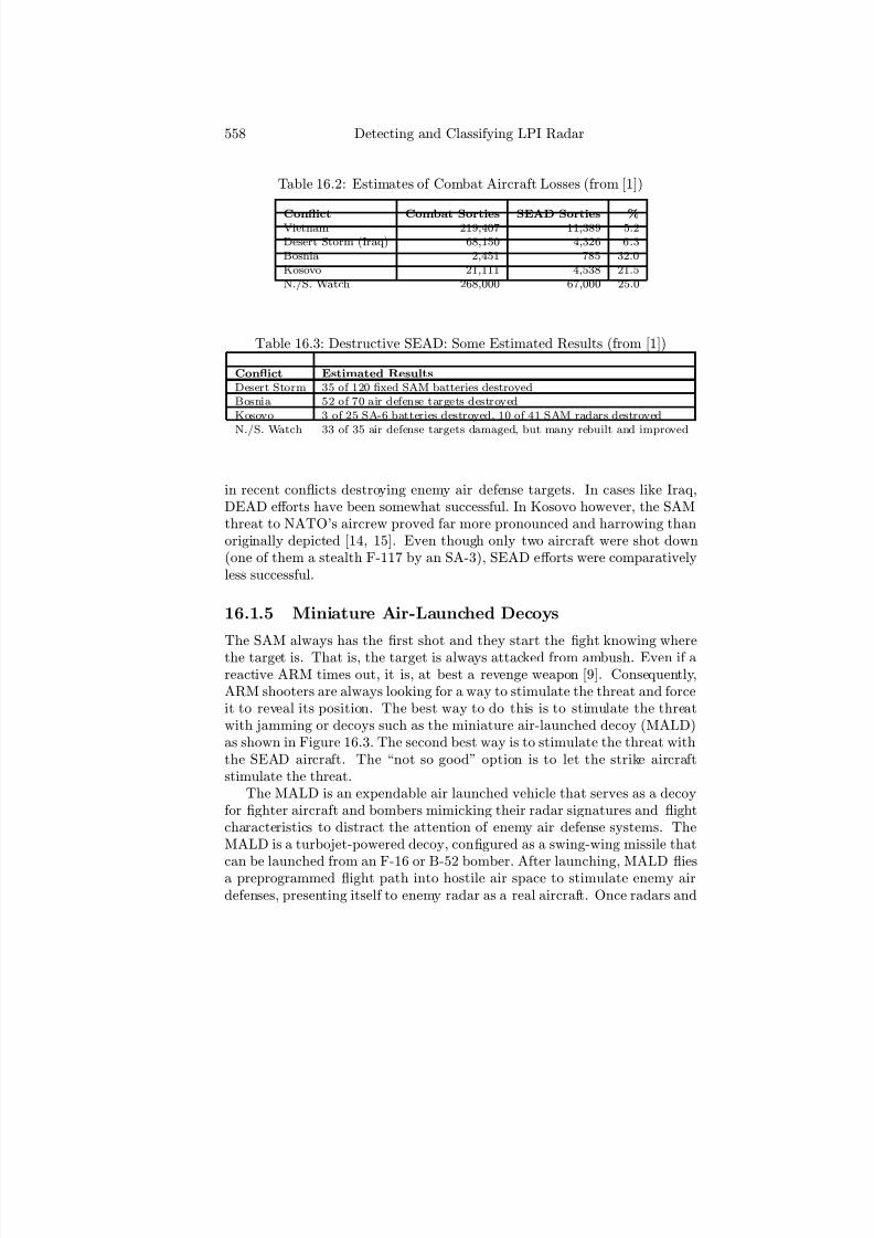
7/17/2019 1596932341 Intercept Radar.pdf
http://slidepdf.com/reader/full/1596932341-intercept-radarpdf 589/891
558 Detecting and Classifying LPI Radar
Table 16.2: Estimates of Combat Aircraft Losses (from [1])
Conflict Combat Sorties SEAD Sorties %Vietnam 219,407 11,389 5.2Desert Storm (Iraq) 68,150 4,326 6.3Bosnia 2,451 785 32.0Kosovo 21,111 4,538 21.5N./S. Watch 268,000 67,000 25.0
Table 16.3: Destructive SEAD: Some Estimated Results (from [1])
Conflict Estimated Results
Desert Storm 35 of 120 fixed SAM batteries destroyedBosnia 52 of 70 air defense targets destroyedKosovo 3 of 25 SA-6 batteries destroyed, 10 of 41 SAM radars destroyed
N./S. Watch 33 of 35 air defense targets damaged, but many rebuilt and improved
in recent conflicts destroying enemy air defense targets. In cases like Iraq,DEAD eff orts have been somewhat successful. In Kosovo however, the SAMthreat to NATO’s aircrew proved far more pronounced and harrowing thanoriginally depicted [14, 15]. Even though only two aircraft were shot down(one of them a stealth F-117 by an SA-3), SEAD eff orts were comparativelyless successful.
16.1.5 Miniature Air-Launched Decoys
The SAM always has the first shot and they start the fight knowing wherethe target is. That is, the target is always attacked from ambush. Even if areactive ARM times out, it is, at best a revenge weapon [9]. Consequently,ARM shooters are always looking for a way to stimulate the threat and forceit to reveal its position. The best way to do this is to stimulate the threatwith jamming or decoys such as the miniature air-launched decoy (MALD)as shown in Figure 16.3. The second best way is to stimulate the threat withthe SEAD aircraft. The “not so good” option is to let the strike aircraftstimulate the threat.
The MALD is an expendable air launched vehicle that serves as a decoyfor fighter aircraft and bombers mimicking their radar signatures and flightcharacteristics to distract the attention of enemy air defense systems. TheMALD is a turbojet-powered decoy, configured as a swing-wing missile that
can be launched from an F-16 or B-52 bomber. After launching, MALD fl
iesa preprogrammed flight path into hostile air space to stimulate enemy airdefenses, presenting itself to enemy radar as a real aircraft. Once radars and

7/17/2019 1596932341 Intercept Radar.pdf
http://slidepdf.com/reader/full/1596932341-intercept-radarpdf 590/891
Antiradiation Missiles 559
Figure 16.3: Miniature air-launched decoy.
air defenses are activated they are intercepted by high speed antiradiationweapons
16.2 Antiradiation Missile Seeker Design
The ARM seeker competes with the warhead for valuable finance, weight andvolume and presents a significant trade-off to the ARM designer. After all,in the endgame, it’s the warhead that counts [16]. However, if the seekerdoes not guide correctly to the target, more serious fratricide problems canoccur. Protected by a wideband RF transparent radome, ARM seekers usepassive RF homing with an antenna and microwave receiver. The antennaand receiver are tuned to the frequency of the threat radar to acquire andprovide location data that can be processed to derive guidance commands.The guidance commands are passed to the missile’s autopilot that filters
the signals to produce guidance and control commands that are sent to thecontrol surfaces. Stability and control of the flight path are then provided bythe control surfaces. An ARM may have a mid-course as well as a terminalphase of the flight.
16.2.1 Antenna Design
The ARM must detect and track the radar radiation over a very broad band-width. It must also have a wide beamwidth in order to detect the emittersat large angles off boresight. Spiral antennas are frequency independent an-tennas that can be used to obtain dual-polarized, rotationally symmetric,multiple-mode patterns over a very broad frequency range [17]. Frequencyindependent antennas are antennas whose geometries are specified by angles
and their radiation pattern, impedance and polarization remain virtually un-changed over a large bandwidth. These features make antennas such as thelogarithmic and conical spirals a good choice for the ARM seeker. They can

7/17/2019 1596932341 Intercept Radar.pdf
http://slidepdf.com/reader/full/1596932341-intercept-radarpdf 591/891
560 Detecting and Classifying LPI Radar
also be implemented with printed circuit technology with a simple microstripfeed network topology that facilitates ease of fabrication [18]. Being confor-mal with the skin of the airframe and not consuming the internal volume of the nose cone can also be an asset when dual-mode seekers are considered.They can also be fixed in place within the nose, do not require a high-precisiongimbal and provide a low cost approach [16].
The antenna performance is not constant for all frequencies. There arephysical bounds that limit the band over which the performance can be heldalmost constant [19]. The performance varies over the bandwidth in a mannerthat is periodic with the logarithm of the frequency. Consequently, they arecalled logarithmically periodic or log-periodic antennas. The most popular of those have shapes prescribed by logarithmic spiral curves or log-spirals. As anexample, a logarithmic uniplanar spiral antenna that covers a 9:1 bandwidthwith a return loss better than 10 dB from 0.4 GHz to 3.8 GHz is describedin [20].
The logarithmic spiral antenna has N arms interleaved in a spiral patternabout the center. Their electrical dimensions however scale with frequency.The feed network at the center of the antenna acts as a beamformer andsplits the power into the arms with a linear progression in phases and equalamplitudes to produce the various modes of radiation. Radiation occurs fromthe points on the spiral which have a half-wavelength in transmission linebetween them. Therefore higher frequencies radiate from the antenna near thecentral feed point and lower frequencies from the edges. The mutual couplingbetween arms relates the excitations at the feed ports to the eff ective patternradiated by each arm. An N = 2-arm spiral consists of two interleaved armswound in a spiral, each terminated in a resistance. N arm spiral antennasare rotationally symmetric such that the rotation of an arm about its axis by2π/N does not change the spiral structure [17]. An N arm spiral can radiate
or receive N − 1 independent (characteristic) modes.The shape of right-handed planar log-spiral antenna is shown in
Figure 16.4 and is based upon the logarithmic spiral curve defined by thegenerating equation [21]
ρ = ρ0ea(φ−φ0) (16.1)
where ρ is the radial distance from the origin in the direction given by theangle φ, and ρ0 is the radius for φ = φ0. For a logarithmic spiral, a is aconstant that controls the flare rate of the spiral (1/a is the spiral rate or rateof expansion of the spiral). We note that the spiral constant
a = 1
ρ
dρ
dφ = cotψ (16.2)
where ψ is the angle between a tangent to the curve at any point and a lineto the origin at that point. Since ψ is constant for a given logarithmic spiral,an alternative name is equiangular spiral [22].
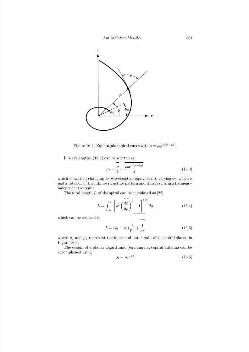
7/17/2019 1596932341 Intercept Radar.pdf
http://slidepdf.com/reader/full/1596932341-intercept-radarpdf 592/891
Antiradiation Missiles 561
Figure 16.4: Equiangular spiral curve with ρ = ρ0ea(φ−φ0).
In wavelengths, (16.1) can be written as
ρλ = ρ
λ =
ρ0ea(φ−φ0)
λ (16.3)
which shows that changing the wavelength is equivalent to varying φ0, which is
just a rotation of the infi
nite structure pattern and thus results in a frequencyindependent antenna.The total length L of the spiral can be calculated as [22]
L =
ρ1ρ0
ρ2dφ
dρ
2
+ 1
1/2dρ (16.4)
which can be reduced to
L = (ρ1 − ρ0)
1 +
1
a2 (16.5)
where ρ0 and ρ1 represent the inner and outer radii of the spiral shown inFigure 16.4.
The design of a planar logarithmic (equiangular) spiral antenna can beaccomplished using
ρ1 = ρ0eaφ (16.6)

7/17/2019 1596932341 Intercept Radar.pdf
http://slidepdf.com/reader/full/1596932341-intercept-radarpdf 593/891
562 Detecting and Classifying LPI Radar
Figure 16.5: Two-arm equiangular spiral plate (adapted from [21]).
as edge number 1 (see Figure 16.4). Edge number 2 has the same spiral curvebut is rotated through a rotation angle δ as
ρ2 = ρ0ea(θ−δ) (16.7)
The other half of the antenna has edges that make the structure symmetric
(opposite configuration) [21]. Rotating one spiral arm by one-half turn bringsit into congruence with the other arm. This assures the antenna can receivesignals of either right-hand polarization or left-hand polarization. A two-armspiral has φ0 = 0,π.
The generating equations for the congruent spiral are
ρ3 = ρ0ea(φ−π) (16.8)
andρ4 = ρ0e
a(φ−π−δ) (16.9)
The structure is shown in Figure 16.5 and is self-complementary containinga good degree of pattern symmetry with δ = π/2.
The frequency of the spiral antenna at the upper end of the operating
band f u is determined by the feed structure [21]. For a = 0.221, the minimumradius ρ0 ≈ λ/4 at f u. A nearly equivalent criterion is that the circumferencein the feed region C u = 2πρ0 = c/f u. The circumference of a circle just

7/17/2019 1596932341 Intercept Radar.pdf
http://slidepdf.com/reader/full/1596932341-intercept-radarpdf 594/891
Antiradiation Missiles 563
Figure 16.6: Archimedean spiral antenna with left hand circular polarization(radiation out of the page) [21] ( cJohn Wiley & Sons, Inc. 1997).
enclosing the spiral can be used to set the low frequency limit f l as C l =2πρ = c/f l. The low frequency limit set by the overall radius is approximatelya quarter wavelength at f l. For example, consider a spiral with one and onehalf turns with a = 0.221. Here the maximum radius R = ρ(φ = 3π) = 8.03ρ0
which is c/4f l. At the feed point R = ρ
(φ0) =
ρ0 = c/4f u. The bandwidth isthen f u/f l = 8 which indicates an 8:1 bandwidth (a typical value).
To maintain a large bandwidth, the antenna must also be fed by an elec-trically and geometrically balanced line. This feed is often referred to as anin fi nite balun and has an impedance of Z ≈ 120Ω [21]. The radiation patternof the self-complementary planar equiangular spiral antenna is bidirectionalwith two wide beams broadside to the plane of the spiral. The filed patternis approximately cos θ when the z-axis is normal to the plane of the spiral.The half-power beamwidth is thus approximately 90o and the polarization isnear circular over wide angles. Spiral antenna gain values range between 2and 4 dB. The frequency limit is typically 500 MHz to 18 GHz.
In the Archimedean spiral antenna, named after the third-century B.C.Greek mathematician Archimedes, the radial distance ρ is linearly propor-
tional to the polar angle φ in the generating equation (rather than exponen-tially related). It flares more slowly as shown in Figure 16.6. The generating

7/17/2019 1596932341 Intercept Radar.pdf
http://slidepdf.com/reader/full/1596932341-intercept-radarpdf 595/891
564 Detecting and Classifying LPI Radar
Figure 16.7: Cutaway view of the programmable wideband British alarmshowing the seeker and spiral antennas.
equations for the Archimedean spiral antenna are
ρ = ρ0φ (16.10)
andρ = ρ0(φ− π) (16.11)
The successive turnings of the spiral have a constant separation distance(equal to 2πρ0 if φ is measured in radians). The arms are fed 180o out-of-phase at F 1 and F 2 giving the antenna circular polarized radiation which isfrequency independent. The radiated fields created by the currents are or-thogonal, equal in magnitude and 90o out of phase. A unidirectional beamcan be created by backing the spiral with a metallic cavity behind the spi-ral. The pattern of the cavity-backed Archimedean spiral can be modeledempirically by [21]
F (θ) = cos5.8(0.53θ) (16.12)
and has a half power beamwidth of 74o. Figure 16.7 shows a schematiccutaway drawing of the British alarm ARM and shows the use of four planarArchimedean spirals to cover the quadrants of interest.
Conical equiangular spirals are also often used in ARM seekers since theygenerate a unidirectional pattern. Figure 16.8 shows the schematic of a conicalequiangular spiral. The edges of one conical spiral surface are defined as

7/17/2019 1596932341 Intercept Radar.pdf
http://slidepdf.com/reader/full/1596932341-intercept-radarpdf 596/891
Antiradiation Missiles 565
Figure 16.8: The conical equiangular spiral antenna [21] ( cJohn Wiley &Sons, Inc. 1997).
ρ = e(a sin θh)φ (16.13)
of which the planar spiral is a special case with θh = 90o. Larger values of θh in 0 ≤ θh ≤ π/2 represent less tightly wound spirals [22]. The generatingequations for the conical equiangular spiral are
ρ1 = e
(a sin θh)φ
(16.14)ρ2 = e(a sin θh)(φ−δ) (16.15)
and δ = π/2 for the self-complementary configuration. The edges of the armsmaintain a constant angle α with a radial line for any cone half-angle θh
a = cotα (16.16)
The advantage to the conical spiral is that it provides a unidirectional ra-diation (single lobe) toward the apex of the cone with the maximum alongthe axis. It also preserves the circular polarization and relatively constantimpedances over the large bandwidths required [22]. Typical patterns forθh ≤ 15o and α ≈ 70o have half-power beamwidths of 80o. For the band de-sign, the apex diameter determines the upper frequency d = c/4f u. The lower
frequency of the antenna is determined by the base diameter B = 3c/(8f l)[21]. As an example of a conical spiral, the Russian Kh-31 ARM uses an arrayof seven conical elements as shown in Figure 16.9.

7/17/2019 1596932341 Intercept Radar.pdf
http://slidepdf.com/reader/full/1596932341-intercept-radarpdf 597/891
566 Detecting and Classifying LPI Radar
Figure 16.9: Photo of the Kh-31 seeker that uses a series of seven conicalspiral elements.
Several patents have been issued that address the shortcomings of spiralantenna designs for ARM seekers. Methods to counteract the threat of theradar shutting down and to also improve the boresight error of the antennasystem and also reduce the radome error slope are reported in [23, 24]. Herethe antenna system includes a parabolic reflector dish having a dielectricsubstrate and a conductive material coating on the substrate in order toprovide a narrowbeam high-gain radiation pattern. The parabolic dish also
has a conductive material coating on the reflector substrate defining the spiralantenna for a low-gain, wideband radiation pattern. To address couplingbetween the antenna and the missile body in the VHF band, a broadbandpolarization diverse monopulse spiral antenna with a body cancelled currentarray and radial arm-coupled log periodic loop antenna is described in [25].To provide a novel nonobvious solution to the problem of fitting a number of spiral antennas having diff erent configuration senses into the space of a singlespiral, the spirals can be symmetrically arranged about a point at the centerof a circle. Each spiral antenna is deformed to occupy substantially all of thearea within a sector of the circle [26].
16.2.2 Receiver and Signal Processing
A block diagram of an ARM including its seeker is shown in Figure 16.10[27]. In this example, the receiver (RX) accepts signals from four antennas
7/17/2019 1596932341 Intercept Radar.pdf
http://slidepdf.com/reader/full/1596932341-intercept-radarpdf 598/891
Antiradiation Missiles 567
that are used to intercept and direction find the RF emission from the radar.Many designs include both a high-band and low-band antenna to improve thedirection finding accuracy (smaller beamwidth). The frequency synthesizer isused to scan the instantaneous bandwidth through the operating bandwidthin order to search for the target radiation. The intercepted emissions aredown-converted, and filtered with a passband filter.
Logarithmic amplification is used in the RX and applied to the passbandfilter output. Logarithmic amplifiers are used widely in antiradiation seek-ers and can be classified into two primary families, the logarithmic IR/RFamplifiers and the detector logarithmic video amplifiers (DLVA) [28]. Thelogarithmic IF/RF amplifier obtains the logarithmic transfer function at theIF (or RF) frequencies, while the DLVA obtains the logarithmic transfer func-tion in the video frequency domain. Advantages of the logarithmic IF ampli-fiers over the DLVA include an easily obtainable CW response (important inARMs attacking LPI emitters), excellent pulse recovery time, fast rise time
and wide instantaneous dynamic range. The DLVA, however, generally hasa smaller logarithmic error over the temperature range and frequencies of in-terest. The DLVA has superior dual-channel tracking characteristics and isusually the choice for ARM monopulse direction finding. This is because itis easier to produce matched nonlinear circuits at video frequencies than atIF/RF frequencies [28].
The amplifier output is lowpass-filtered and the monopulse azimuth (AZ)and elevation (EL) error signals are digitized. Also digitized are the RFfrequency, the pulse time of arrival (TOA), the pulse width (PW), and theamplitude of the pulse. The signal processing then gates these error signalsand uses pulse discriminant logic, deinterleaving, and a PRF correlator in or-der to sort the various radar signals being intercepted including their angularlocation. A Kalman filter is then used to derive the command acceleration
from the seeker line of sight rate on the selected target signal. The autopilotthen filters these commanded accelerations, which are then applied perpen-dicular to the airframe velocity vector to guide the missile to the target.
16.2.3 Dual-Mode Design
There are two major problems that aff ect ARM performance. The first consid-eration is that air defense radars, when anticipating an ARM attack, usuallyoperate in a blink mode turning on just long enough to obtain tactical infor-mation then shutting down to avoid attracting ARMs. The second problemis that if the radar stays active allowing the ARM to be launched againstit, some attacks will fail because some of the radar energy bounces off theground creating a false (multipath) target [29]. If the multipath is not too
severe, the problem can be addressed using leading-edge track. To addressmore significant multipath situations and also counter the blink mode theconcept of the dual-mode ARM seeker has been explored.

7/17/2019 1596932341 Intercept Radar.pdf
http://slidepdf.com/reader/full/1596932341-intercept-radarpdf 599/891
568 Detecting and Classifying LPI Radar
Figure 16.10: Block diagram of an antiradiation missile seeker (from [27]).

7/17/2019 1596932341 Intercept Radar.pdf
http://slidepdf.com/reader/full/1596932341-intercept-radarpdf 600/891
Antiradiation Missiles 569
Dual-mode ARM seekers can increase the capability of the missile whenthe RF radiation source shuts down. A unique dual-mode guidance schemedevised by the U.S. Army researchers was key to developing a more eff ectiveARM with a minimal increase in cost and weight. The dual-mode seekerwould retain the traditional passive mode RF homing capability but wouldalso have either an imaging infrared or active millimeter wave (MMW) radarmode. These latter modes do not require radar emissions from the targetand can deal with blink tactics . They can also give higher accuracy whenused in the final stage of the attack. The addition of a second guidancemode involves additional hardware increasing the manufacturing costs of themissile. Note that the design and production of ARMs represent a balancebetween the technology that is incorporated into the missile and the abilityof the manufacturer to sell the weapon system.
The solution proposed by the U.S. Army is based on an active MMWseeker, but adds to that seeker antiradiation homing antennas and down
conversion elements as shown in Figure 16.11. The antiradiation homing an-tennas intercept signals emitted by enemy air defense radar but instead of passing these signals to a dedicated receiver and guidance system, the an-tennas pass them to the conversion elements. The task of these conversionelements is to convert the intercepted signals to the IF that is also used by theactive MMW processing. This IF could then be handled by the signal proces-sor that already exists as part of the MMW seeker. Use of the same processorto handle both passive and active-mode radar signals greatly reduces the costpenalties of providing the second guidance mode.
At least three or four passive detector channels should be used. The as-sociated antennas would be mounted on the exterior of the missile at regularintervals around the circumference of the fuselage. With proper phase rela-tionships between detector channels the azimuth and elevation direction find-
ing (DF) information can be provided. The antennas should have a broadbeamwidth so phase comparison monopulse techniques can be used ratherthan the alternative amplitude comparison DF technique. The angle of ar-rival of the enemy radar signal would be determined by comparing the phaseof the emission signals from the individual antennas.
During the initial and mid-course portions of flight the dual-mode mis-sile would use its passive-radar mode to home in on the emissions from thehostile radar. During the terminal phase of the attack, it would switch tothe active MMW mode, acquire the hostile radar and conduct an accurateattack that does not depend on the target remaining active. The distancefrom the target at which the missile switches modes is a function of its speedand maneuverability and is typically 2—4 km.
Another example of a dual-mode ARM seeker is Alliant Techsystem’s
advanced antiradiation guided missile (AARGM) shown in Figure 16.12. De-veloped under the Navy’s Quick Bolt program, the passive conformal arrayantenna provides high accuracy wideband DF capability [30]. Autonomous

7/17/2019 1596932341 Intercept Radar.pdf
http://slidepdf.com/reader/full/1596932341-intercept-radarpdf 601/891
570 Detecting and Classifying LPI Radar
Figure 16.11: MMW/Passive detector channels diagram.
target detection, identification, tracking and location ranging of the targetare provided. The large field of view, sensitivity, frequency and DF accuracyand processing enable the weapon to be successful without an independenttargeting system.
In addition to homing in on the signal emitted by the hostile radar, theAARGM’s dual-mode guidance includes an active MMW radar. This sectionof the seeker provides terminal target acquisition, tracking, guidance andfusing to find its target even if the hostile radar is no longer radiating (anti-ARM tactics). If the radar shuts down, the MMW will go into a searchmode. Since the seeker is in the MMW band it can detect RF scattering fromthe radar antenna, radar platform and missile launcher [30]. An integratedGPS/INS navigation suite is also included in the seeker to provide mid-courseguidance and supply the rough coordinates to fly to after the radar shutsdown. This prevents the ARM from missing the target in the terminal phaseand most importantly, keeps the weapon from landing in the wrong country(preventing fratricide) [13]. It also enables a sensor fusion and autonomousranging capability.
These features extend the AARGM capability providing a long-range,time-critical strike weapon against other than the traditional ARM radar
targets. That is, the warfi
ghter survivability is increased with the addi-tional speed, range and targeting capability. The AARGM weapon also hasa network-enabled capability with a receiver that links the weapon to na-
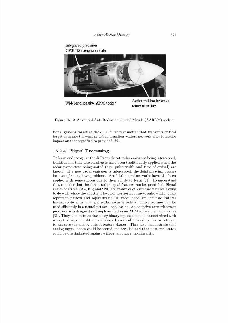
7/17/2019 1596932341 Intercept Radar.pdf
http://slidepdf.com/reader/full/1596932341-intercept-radarpdf 602/891
Antiradiation Missiles 571
Figure 16.12: Advanced Anti-Radiation Guided Missile (AARGM) seeker.
tional systems targeting data. A burst transmitter that transmits criticaltarget data into the warfighter’s information warfare network prior to missileimpact on the target is also provided [30].
16.2.4 Signal Processing
To learn and recognize the diff erent threat radar emissions being intercepted,traditional if-then-else constructs have been traditionally applied when theradar parameters being sorted (e.g., pulse width and time of arrival) areknown. If a new radar emission is intercepted, the deinterleaving processfor example may have problems. Artificial neural networks have also beenapplied with some success due to their ability to learn [31]. To understandthis, consider that the threat radar signal features can be quantified. Signalangles of arrival (AZ, EL) and SNR are examples of extrinsic features havingto do with where the emitter is located. Carrier frequency, pulse width, pulserepetition pattern and sophisticated RF modulation are intrinsic featureshaving to do with what particular radar is active. These features can beused efficiently in a neural network application. An adaptive network sensorprocessor was designed and implemented in an ARM software application in[31]. They demonstrate that noisy binary inputs could be characterized withrespect to noise amplitude and shape by a recall procedure that was tuned
to enhance the analog output feature shapes. They also demonstrate thatanalog input shapes could be stored and recalled and that unstored statescould be discriminated against without an output nonlinearity.
7/17/2019 1596932341 Intercept Radar.pdf
http://slidepdf.com/reader/full/1596932341-intercept-radarpdf 603/891
572 Detecting and Classifying LPI Radar
In summary, modern microelectronic technology has made it possible toput immensely sophisticated detection and analysis systems into the ARM.Each missile carries its own radar seeker, signal analysis equipment and athreat file, which enables it to identify virtually any radar by its signalstructure—frequency, pulse length, modulation and pulse repetition frequency.The ARM can leave the launch aircraft and search for radar signals, compar-ing received pulses with a comprehensive threat file, in order to find and thenhome onto the greatest hostile threat. With the loiter capability (e.g., HARMand Alarm), the ARM can climb to altitude, deploy a parachute and thensearch for target signals as it descends slowly.
Once a target has been identified, a high-speed attack phase is initiated,which enables the missile to get to the target in a very short time. Both typeshave inertial navigation systems which can store positions from which signalshave been detected, and then guide the missile to the selected target withoutfurther signal inputs. Switching off the radar provides little protection against
this sort of capability. In any case, radar is a fundamental part of manyair defense systems, often providing direct control of anti-aircraft missiles inaddition to detecting and tracking targets. Such radar systems must havea high priority in the threat file carried by any antiradiation missile andswitching off the radar for self-protection will render the complete missilesystem ineff ective. Partly as a result of this, there is a steadily increasingemphasis on highly mobile radar systems although mobility is unlikely toprovide a defense against an imminent attack. If an ARM has already beenlaunched from an aircraft, the amount of warning will be measured in seconds.If the launch aircraft pops up over the radar horizon, detects a hostile radaremission and then launches an ARM, the radar will have its first warningof the attack when it is only about 15 km away. This would probably giveit between 10 and 20 seconds to reorganize. As shown in Figure 16.13 the
F-4G Wild Weasel can carry an air-to-ground missile (AGM)–AGM-88 high-speed ARM (HARM); the AGM-65 Maverick, which has an infrared seeker;the ALQ-119 electronic attack pod; the AGM-78 Standard ARM; and theAGM-45 Shrike ARM.
16.2.5 Future ARMs–Addressing the LPI Emitter
Until recently, almost all radars were designed to transmit short-durationpulses with a high peak power. This type of signal is easy to detect usingrelatively simple, traditional ARM seeker receivers as shown in Figure 16.10making the radar source vulnerable to an ARM attack. With the arrival of theLPI requirements, the ARM seeker and signal processing methodology mustbe revisited. The use of very low peak power (e.g., P CW = 1 mW) requires
the ARM seeker to have a much higher sensitivity in order to detect thesetypes of signals. With the increasing number of radars using LPI techniques,the ARM is now required to measure and characterize conventional pulsed

7/17/2019 1596932341 Intercept Radar.pdf
http://slidepdf.com/reader/full/1596932341-intercept-radarpdf 604/891
Antiradiation Missiles 573
Figure 16.13: F-4G Wild Weasel carrying an AGM-88 HARM, AGM-65 Mav-erick, ALQ-119 electronic attack pod, AGM-78 Standard ARM, and an AGM-45 Shrike ARM.
radar signals as well as detect and characterize the LPI signals.Detection of LPI signals can be accomplished using a number of diff erent
receiver architectures. The signal processing functions can be quite intensiveif all of the received data (pulsed waveforms and LPI waveforms) is digitizedat the IF band and analyzed using signal processing. Figure 16.14 shows an
example of an LPI signal, a pulsed emitter signal and the presense of thermalnoise within the ARM seeker.
A solution to the problem of overloading the signal processor when LPIsignals are present along with pulsed waveforms can be addressed with anLPI signal discriminator. A block diagram of the discriminator is shown inFigure 16.15. The LPI signal discriminator is operatively coupled to the downconverter and produces a trigger signal that is used when the incoming signalis above a predetermined threshold, to thereby transfer the digitized signalto a special digital signal processor for analyzing the incoming LPI signal.The architecture suppresses the high-peak power, short duration signals andtriggers a data buff er for gating the digitized LPI data to the digital signalprocessor [32]. The LPI signal discriminator in an analog processor uses acascade of IF amplifiers with a pad between the amplifiers to distribute thesignal power evenly throughout the chain and soft-limit the strong pulsedsignals that are received. The amplified signal is detected by a large dynamic

7/17/2019 1596932341 Intercept Radar.pdf
http://slidepdf.com/reader/full/1596932341-intercept-radarpdf 605/891
574 Detecting and Classifying LPI Radar
Figure 16.14: LPI and pulsed signal amplitudes within an ARM seeker as a
function of time (from [32]).
range, successive detector log video amplifier. The logarithmic video outputis further compressed using a follow-on video logarithmic amplifier before thesignal is time-integrated by one or more integrators. A threshold comparatorreceives the output from the integrators to provide a trigger pulse outputwhen the input crosses a predetermined threshold value set by the signalprocessor [32].
The LPI emitter can also be detected with a sufficient amount of inte-gration of the intercepted energy. For each direction of arrival, an optimaldetector is able to integrate the energy of the emitted signal of which theparameters are unknown. Using a multichannel detector, the diff erent chan-
nels can be tuned onto diff
erent durations and passbands for the noncoherentintegration. The output of each channel depends on the time of arrival andthe starting spectrum frequency. Searching for the emitter in time and fre-quency is most conveniently done in the time-frequency domain which is easilycalculated as shown in the previous chapters.
A multichannel detection algorithm recently suggested for time-frequencydomain LPI detection is given as [33]
ξ ( p, q ) =
t0+T t=t0
f 0+Bf =f 0
|G(t, f )|2 (16.17)
which uses the Gabor time-frequency distribution G where t0 is the signal’stime of arrival, f 0 is the initial spectrum frequency, T is the signal duration
and B is the signal bandwidth. This noncoherent integration is done usingtwo-dimensional sliding windows as shown in Figure 16.16 [34]. In Figure16.16(a) a model of the time domain signals within the receiver are shown

7/17/2019 1596932341 Intercept Radar.pdf
http://slidepdf.com/reader/full/1596932341-intercept-radarpdf 606/891
Antiradiation Missiles 575
Figure 16.15: Block diagram of an analog LPI signal discriminator (adaptedfrom [32]).
Figure 16.16: (a) Time domain and frequency domain model of the thermalnoise and LPI emitter signal and (b) two examples of a noncoherent integra-tion sliding window for detection of the LPI signal (adapted from [34]).

7/17/2019 1596932341 Intercept Radar.pdf
http://slidepdf.com/reader/full/1596932341-intercept-radarpdf 607/891
576 Detecting and Classifying LPI Radar
Figure 16.17: Block diagram of a digital FMCW signal discriminator (adaptedfrom [35]).
and include the LPI signal x(t) and the receiver’s thermal noise n(t) in thetime domain and the magnitude spectrum |X (f )| and |N (f )| in the frequencydomain.
Another architecture for detecting FMCW LPI waveforms employs a tech-nique described as “deramping” which forms an adaptive matched filter tothe linear FMCW signal in order to achieve the processing gain that is equalto the LPI signal’s time-bandwidth product [35]. A block diagram of thistechnique is shown in Figure 16.17. The deramping process mixes the inputsignal with a locally generated linear FM signal to produce an output signalwith a reduced FM slope in comparison with the input signal. To construct amatched filter, the carrier frequency, modulation period and the modulationbandwidth must be known. To determine these parameters, the matchedfilter must be adaptively formed. A multichannel arrangement is proposedby examining the output of an FFT filter bank using a CFAR scheme thatsets the threshold for determining the channel hit. The channel that yieldsthe first detection has its matched filter parameters adaptively changed toachieve optimal processing gain.
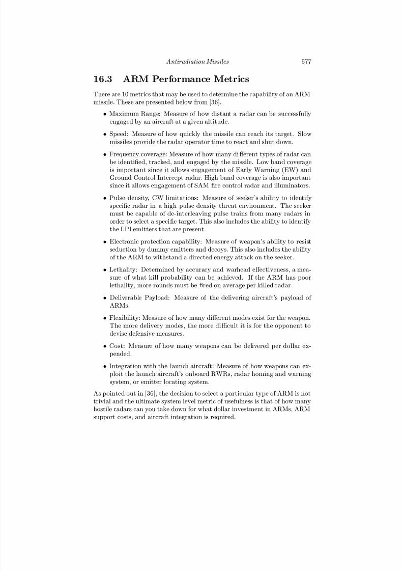
7/17/2019 1596932341 Intercept Radar.pdf
http://slidepdf.com/reader/full/1596932341-intercept-radarpdf 608/891
Antiradiation Missiles 577
16.3 ARM Performance Metrics
There are 10 metrics that may be used to determine the capability of an ARM
missile. These are presented below from [36].
• Maximum Range: Measure of how distant a radar can be successfullyengaged by an aircraft at a given altitude.
• Speed: Measure of how quickly the missile can reach its target. Slowmissiles provide the radar operator time to react and shut down.
• Frequency coverage: Measure of how many diff erent types of radar canbe identified, tracked, and engaged by the missile. Low band coverageis important since it allows engagement of Early Warning (EW) andGround Control Intercept radar. High band coverage is also importantsince it allows engagement of SAM fire control radar and illuminators.
• Pulse density, CW limitations: Measure of seeker’s ability to identifyspecific radar in a high pulse density threat environment. The seekermust be capable of de-interleaving pulse trains from many radars inorder to select a specific target. This also includes the ability to identifythe LPI emitters that are present.
• Electronic protection capability: Measure of weapon’s ability to resistseduction by dummy emitters and decoys. This also includes the abilityof the ARM to withstand a directed energy attack on the seeker.
• Lethality: Determined by accuracy and warhead eff ectiveness, a mea-sure of what kill probability can be achieved. If the ARM has poorlethality, more rounds must be fired on average per killed radar.
• Deliverable Payload: Measure of the delivering aircraft’s payload of ARMs.
• Flexibility: Measure of how many diff erent modes exist for the weapon.The more delivery modes, the more difficult it is for the opponent todevise defensive measures.
• Cost: Measure of how many weapons can be delivered per dollar ex-pended.
• Integration with the launch aircraft: Measure of how weapons can ex-ploit the launch aircraft’s onboard RWRs, radar homing and warningsystem, or emitter locating system.
As pointed out in [36], the decision to select a particular type of ARM is not
trivial and the ultimate system level metric of usefulness is that of how manyhostile radars can you take down for what dollar investment in ARMs, ARMsupport costs, and aircraft integration is required.

7/17/2019 1596932341 Intercept Radar.pdf
http://slidepdf.com/reader/full/1596932341-intercept-radarpdf 609/891
578 Detecting and Classifying LPI Radar
16.4 Former Soviet Union and Warsaw PactAllies
The former Soviet Union and the current Russian Federated States have beendeveloping ARMs since the 1960s. Unlike the United States, the Soviet Uniondid not develop aircraft specialized for SEAD missions. That is, they didnttreat SEAD as independent air operations [37]. The Soviet’s developmentof its ARMs was driven by doctrine of a massive frontal air assault on themost common threat at the time, Western Europe. Since this assault wouldhave numerous aircraft, these ARMs did not have to be sophisticated and nodedicated SEAD aircraft were fielded.
SEAD missions were flown to support air-ops on a tactical level (by non-specialists). They relied on signals intelligence (SIGINT) and other reconassets and preferred preplanned strikes on known enemy IADS rather thantargets of opportunity [37]. With the theater of war in western Europe, the
western SAM threats (late 1950s, early 1960s) consisted of the U.S. NikeAjax, Nike Hercules, U.K. Thunderbird, and the Bloodhound systems. Withthe Ilyushin Il-28 Beagle (nuclear weapon platform) having a cruising speedof only 500 mph, no low-level penetration was attempted. Following this,the Yakovlev Yak-28 (Brewer) supersonic (1960) and Sukhoi Su-7 (Fitter-A)supersonic (1960) also provided no solution to the SAM problem. Instead,the Soviet Union relied on mass nuclear weapons employment. Not until 1963did work begin on the first tactical ARM. Table 16.4 lists the ARM weaponsdeveloped along with their NATO name and year the ARM entered service.
Table 16.4: Russian ARM Development
Mi ssil e NATO code Russi an na me Entered Ser vi ce
AA-10 Alamo R-27P 1989
AS-4 Kitchen Kh-22MP 1974
AS-5 Kelt KSR-2P 1962
AS-6 Kingfish Kh-26MP 1969AS-9 Kyle Kh-28, Kh-28E 1973
AS-11 Kilter Kh-58 1977
AS-12 Kegler Kh-25MP, Kh-25MPU 1981AS-16 Kickback Kh-15P 1988
AS-17 Krypton Kh-31P 1991
16.4.1 AA-10 AlamoThe AA-10 Alamo is an air-to-air missile fitted with a passive seeker thathomes in on the emissions from a threat fighter’s radar. It was fielded in 1989
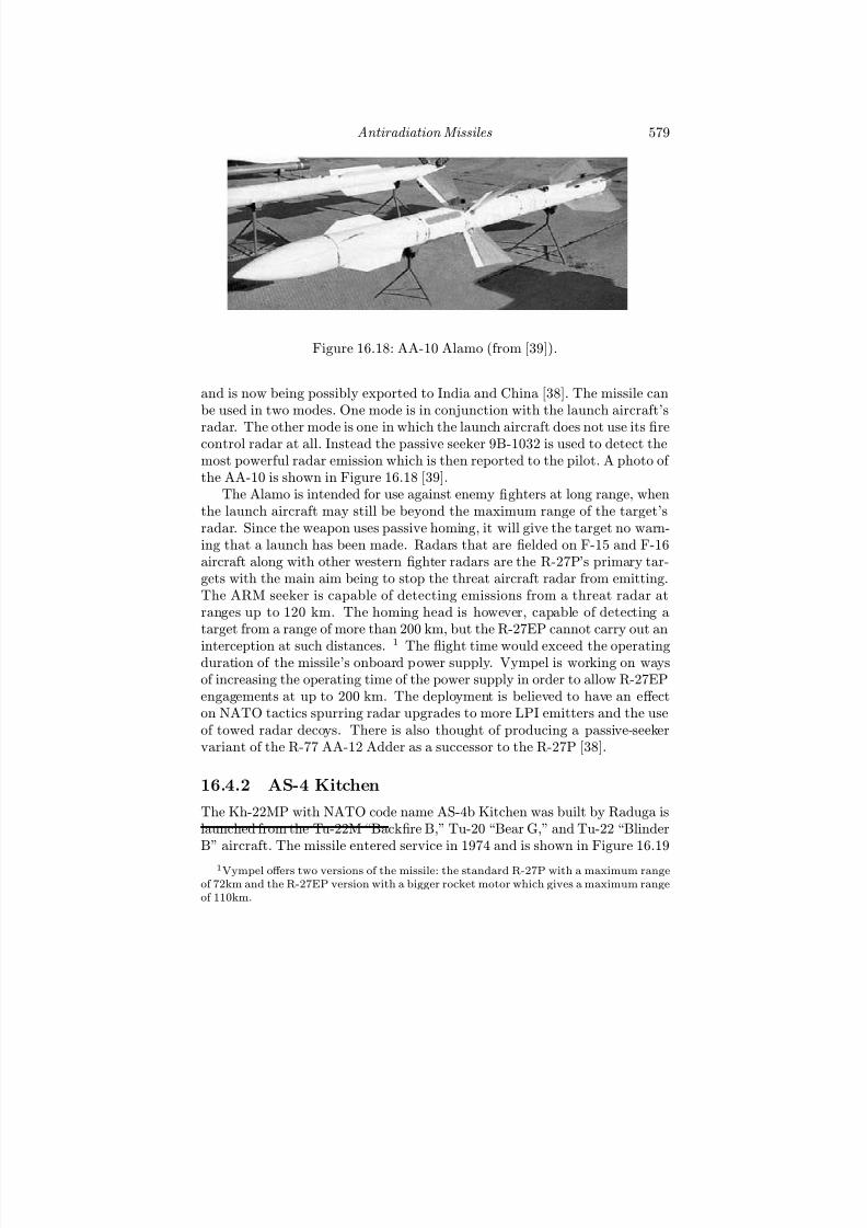
7/17/2019 1596932341 Intercept Radar.pdf
http://slidepdf.com/reader/full/1596932341-intercept-radarpdf 610/891
Antiradiation Missiles 579
Figure 16.18: AA-10 Alamo (from [39]).
and is now being possibly exported to India and China [38]. The missile canbe used in two modes. One mode is in conjunction with the launch aircraft’s
radar. The other mode is one in which the launch aircraft does not use its firecontrol radar at all. Instead the passive seeker 9B-1032 is used to detect themost powerful radar emission which is then reported to the pilot. A photo of the AA-10 is shown in Figure 16.18 [39].
The Alamo is intended for use against enemy fighters at long range, whenthe launch aircraft may still be beyond the maximum range of the target’sradar. Since the weapon uses passive homing, it will give the target no warn-ing that a launch has been made. Radars that are fielded on F-15 and F-16aircraft along with other western fighter radars are the R-27P’s primary tar-gets with the main aim being to stop the threat aircraft radar from emitting.The ARM seeker is capable of detecting emissions from a threat radar atranges up to 120 km. The homing head is however, capable of detecting atarget from a range of more than 200 km, but the R-27EP cannot carry out an
interception at such distances. 1 The flight time would exceed the operatingduration of the missile’s onboard power supply. Vympel is working on waysof increasing the operating time of the power supply in order to allow R-27EPengagements at up to 200 km. The deployment is believed to have an eff ecton NATO tactics spurring radar upgrades to more LPI emitters and the useof towed radar decoys. There is also thought of producing a passive-seekervariant of the R-77 AA-12 Adder as a successor to the R-27P [38].
16.4.2 AS-4 Kitchen
The Kh-22MP with NATO code name AS-4b Kitchen was built by Raduga islaunched from the Tu-22M “Backfire B,” Tu-20 “Bear G,” and Tu-22 “BlinderB” aircraft. The missile entered service in 1974 and is shown in Figure 16.19
1Vympel off ers two versions of the missile: the standard R-27P with a maximum rangeof 72km and the R-27EP version with a bigger rocket motor which gives a maximum rangeof 110km.

7/17/2019 1596932341 Intercept Radar.pdf
http://slidepdf.com/reader/full/1596932341-intercept-radarpdf 611/891
580 Detecting and Classifying LPI Radar
Figure 16.19: Kh-22 Kitchen (from [40]).
[40]. It is used against ship- or ground-based radars and has a 930-kg HEblast fragmentation warhead with an active laser fuse. Guidance is inertialwith a passive radar terminal seeker.
The passive guidance (PG) radar seeker can lock on to a target from adistance of 250—270 km. The inertial guided versions use the PSI Dopplerradar to compute distance covered. The passive radar homing missiles havethe PGP passive radar seeker with a range of 380—350 km [41]. After launchthe missile climbs to an altitude of 22,500m for cruise flight stabilized by the
APK-22A autopilot and then dives into the target at an angle of 30 degrees.Maximum launch range depends on the speed and altitude of the launchingaircraft: from a speed of 950 km/h and an altitude of 10 km it is 400 kmand from a speed of 1,720 km/h and an altitude of 14 km it is 550 km. Theinitial versions of the Kh-22 had a maximum speed of 3,600 km/h, which wasincreased to 4,000 km/h with the Kh-22M series that entered service in 1974and 1976. The Kh-22B experimental version reached a speed of Mach 6 andan altitude of 70 km during tests in the 1970s [41].
16.4.3 AS-5 Kelt
The KSR-2P with NATO code name AS-5 Kelt was built by OKB MiG andcould be launched from the Tu-16 “Badger C mod,” “Badger G” and had a
maximum range of 220 km and a maximum speed of Mach 1.2. The Keltshown in Figure 16.20 entered service in 1962, but was phased out by the late

7/17/2019 1596932341 Intercept Radar.pdf
http://slidepdf.com/reader/full/1596932341-intercept-radarpdf 612/891
Antiradiation Missiles 581
Figure 16.20: An AS-5 Kelt air to surface missile loaded on the wing pylon of an Egyptian Air Force Tu-16 Badger aircraft [42] ( c2007 Jane’s InformationGroup).
1980s [42]. The operational ceiling of the missile was 9.1 km. About 25 Keltswere used by the Egyptian Air Force in 1973 against Israeli forces, and fiveare reported to have been successful. It is believed that 12 of these missileswere anti-radar versions of the AS-5.
16.4.4 AS-6 Kingfish
The KSR-5P with NATO code name AS-6 Kingfish was built by Raduga and
was launched from the Tu-16 “Badger G mod.” It had a maximum range of 400 km with maximum speed of Mach 3.0 [43]. The AS-6 missile as shownin Figure 16.21 entered service in 1969, with a second version in 1973 forcarriage on the Tu-95 “Bear,” and a third version in 1976 for carriage on theTu-95M. There were reported to be around 100 missiles in service in Russiain 1990, but modified missiles were off ered for export as air targets and itis believed that all AS-6s had been removed from operational service by theend of 1994. Some AS-6 missiles were retained by Ukraine, but by 2002 it isbelieved that these missiles had been destroyed. The missile is launched froman altitude of 0.5—11 km after which it climbs to an altitude of 20 km forcruise flight. The missile starts its terminal dive 60 km from the target. Themost recent version, the KSR-5NM also included the ability to loiter whichadded more flexibility to attack SAMs that shut down once the missile was
in the air.
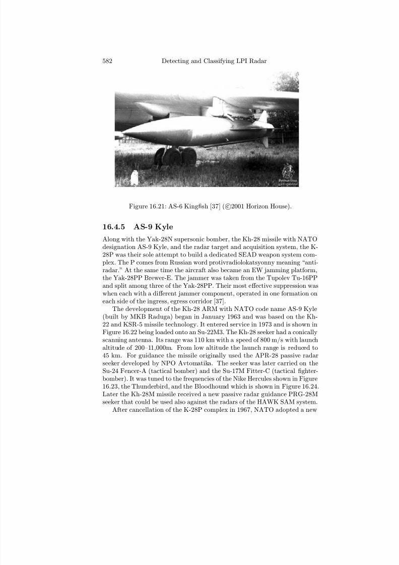
7/17/2019 1596932341 Intercept Radar.pdf
http://slidepdf.com/reader/full/1596932341-intercept-radarpdf 613/891
582 Detecting and Classifying LPI Radar
Figure 16.21: AS-6 Kingfish [37] ( c2001 Horizon House).
16.4.5 AS-9 Kyle
Along with the Yak-28N supersonic bomber, the Kh-28 missile with NATOdesignation AS-9 Kyle, and the radar target and acquisition system, the K-28P was their sole attempt to build a dedicated SEAD weapon system com-plex. The P comes from Russian word protivradiolokatsyonny meaning “anti-radar.” At the same time the aircraft also became an EW jamming platform,the Yak-28PP Brewer-E. The jammer was taken from the Tupolev Tu-16PPand split among three of the Yak-28PP. Their most eff ective suppression was
when each with a diff
erent jammer component, operated in one formation oneach side of the ingress, egress corridor [37].The development of the Kh-28 ARM with NATO code name AS-9 Kyle
(built by MKB Raduga) began in January 1963 and was based on the Kh-22 and KSR-5 missile technology. It entered service in 1973 and is shown inFigure 16.22 being loaded onto an Su-22M3. The Kh-28 seeker had a conicallyscanning antenna. Its range was 110 km with a speed of 800 m/s with launchaltitude of 200—11,000m. From low altitude the launch range is reduced to45 km. For guidance the missile originally used the APR-28 passive radarseeker developed by NPO Avtomatika. The seeker was later carried on theSu-24 Fencer-A (tactical bomber) and the Su-17M Fitter-C (tactical fighter-bomber). It was tuned to the frequencies of the Nike Hercules shown in Figure16.23, the Thunderbird, and the Bloodhound which is shown in Figure 16.24.
Later the Kh-28M missile received a new passive radar guidance PRG-28Mseeker that could be used also against the radars of the HAWK SAM system.After cancellation of the K-28P complex in 1967, NATO adopted a new

7/17/2019 1596932341 Intercept Radar.pdf
http://slidepdf.com/reader/full/1596932341-intercept-radarpdf 614/891
Antiradiation Missiles 583
Figure 16.22: Ground crews prepare to load a AS-9 Kyle (Kh-28) on anSu-22M3 Fitter-F [37] ( c2001 Horizon House).
Figure 16.23: Nike Hercules SAM.
Figure 16.24: Bloodhound Mk 2 SAM deployed on its Type 202 launcher.
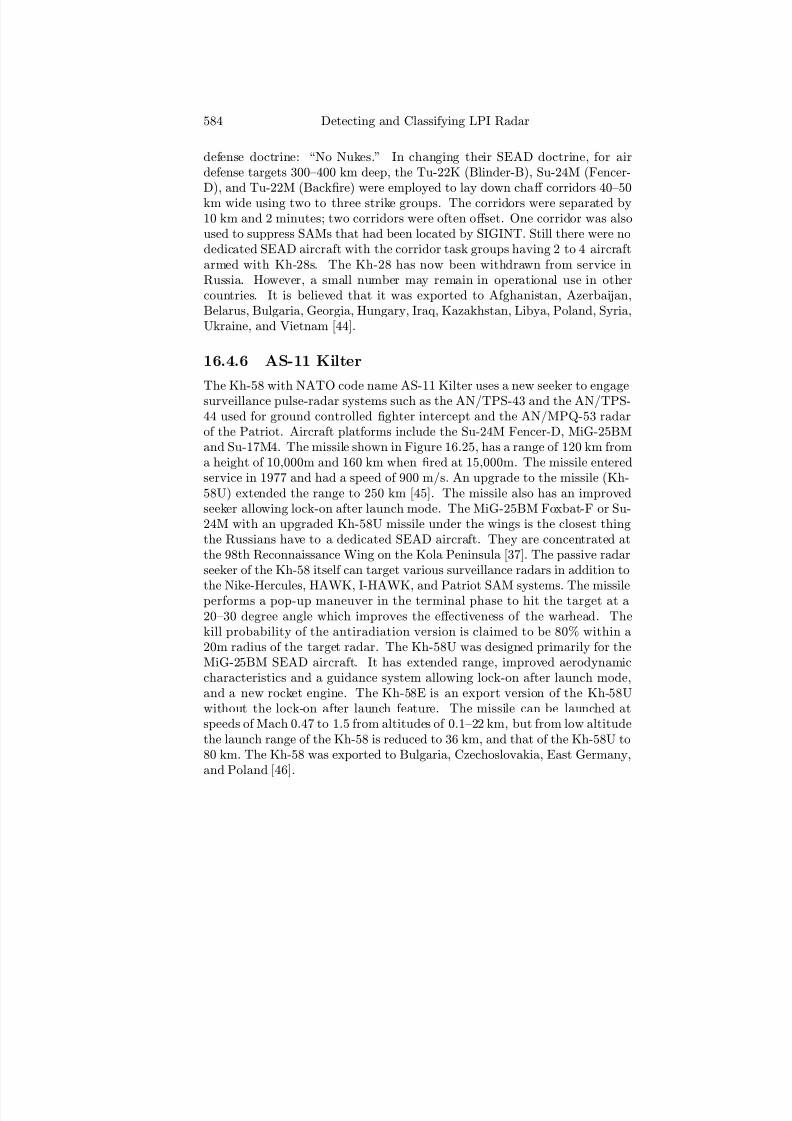
7/17/2019 1596932341 Intercept Radar.pdf
http://slidepdf.com/reader/full/1596932341-intercept-radarpdf 615/891
584 Detecting and Classifying LPI Radar
defense doctrine: “No Nukes.” In changing their SEAD doctrine, for airdefense targets 300—400 km deep, the Tu-22K (Blinder-B), Su-24M (Fencer-D), and Tu-22M (Backfire) were employed to lay down chaff corridors 40—50km wide using two to three strike groups. The corridors were separated by10 km and 2 minutes; two corridors were often off set. One corridor was alsoused to suppress SAMs that had been located by SIGINT. Still there were nodedicated SEAD aircraft with the corridor task groups having 2 to 4 aircraftarmed with Kh-28s. The Kh-28 has now been withdrawn from service inRussia. However, a small number may remain in operational use in othercountries. It is believed that it was exported to Afghanistan, Azerbaijan,Belarus, Bulgaria, Georgia, Hungary, Iraq, Kazakhstan, Libya, Poland, Syria,Ukraine, and Vietnam [44].
16.4.6 AS-11 Kilter
The Kh-58 with NATO code name AS-11 Kilter uses a new seeker to engagesurveillance pulse-radar systems such as the AN/TPS-43 and the AN/TPS-44 used for ground controlled fighter intercept and the AN/MPQ-53 radarof the Patriot. Aircraft platforms include the Su-24M Fencer-D, MiG-25BMand Su-17M4. The missile shown in Figure 16.25, has a range of 120 km froma height of 10,000m and 160 km when fired at 15,000m. The missile enteredservice in 1977 and had a speed of 900 m/s. An upgrade to the missile (Kh-58U) extended the range to 250 km [45]. The missile also has an improvedseeker allowing lock-on after launch mode. The MiG-25BM Foxbat-F or Su-24M with an upgraded Kh-58U missile under the wings is the closest thingthe Russians have to a dedicated SEAD aircraft. They are concentrated atthe 98th Reconnaissance Wing on the Kola Peninsula [37]. The passive radarseeker of the Kh-58 itself can target various surveillance radars in addition to
the Nike-Hercules, HAWK, I-HAWK, and Patriot SAM systems. The missileperforms a pop-up maneuver in the terminal phase to hit the target at a20—30 degree angle which improves the eff ectiveness of the warhead. Thekill probability of the antiradiation version is claimed to be 80% within a20m radius of the target radar. The Kh-58U was designed primarily for theMiG-25BM SEAD aircraft. It has extended range, improved aerodynamiccharacteristics and a guidance system allowing lock-on after launch mode,and a new rocket engine. The Kh-58E is an export version of the Kh-58Uwithout the lock-on after launch feature. The missile can be launched atspeeds of Mach 0.47 to 1.5 from altitudes of 0.1—22 km, but from low altitudethe launch range of the Kh-58 is reduced to 36 km, and that of the Kh-58U to80 km. The Kh-58 was exported to Bulgaria, Czechoslovakia, East Germany,and Poland [46].

7/17/2019 1596932341 Intercept Radar.pdf
http://slidepdf.com/reader/full/1596932341-intercept-radarpdf 616/891
Antiradiation Missiles 585
Figure 16.25: AS-11 Kilter (from [45]).
16.4.7 Kh-27
The Kh-27 antiradiation missile (no NATO designation) has a speed of 850 m/s and was conceived as a replacement for the heavy Kh-28. Conceivedas an ARM variant of the earlier Kh-23 (AS-7 Kerry), the Kh-27 enteredservice in 1977 targeting the Nike Hercules, Thunderbird, Bloodhound andHAWK SAM systems. The missile was carried on aircraft platforms MiG-27and Su-17M3 and had a range of 60 km when launched from 15,000m and40 km from 5,000m. The new seeker was developed with a highly sensitivereceiver with five antennas in the PRGS-1 type guidance version and with sixantennas in the PRGS-2 version. Direction finding to the target was based onphase diff erence interferometry and was much more accurate than the coni-cal scanning antenna in the Kh-28. The weapon saw limited service in thelate 1970s and early 1980s, and was replaced by the ARM member of the“modular” Kh-25M AS-12 Kegler family.
16.4.8 AS-12 Kegler
The Kh-25MP and improved Kh-25MPU with NATO code name AS-12 Kegler(built by Zvezda) are dedicated antiradiation variants of the Kh-25 (AS-10)air-to-surface missile. The missile was given a new NATO code name becauseof its specific defense suppression role. The Kh-25MP eff ectively replaced theKh-28 (AS-9 Kyle) in Russian service. The missile entered service in 1981[47]. The missile shown in Figure 16.26 had two interchangeable seeker headswith antennas tuned to the radar frequencies of the HAWK and Nike Her-cules SAM systems respectively [48]. Targeting was done with the Vyoga ES

7/17/2019 1596932341 Intercept Radar.pdf
http://slidepdf.com/reader/full/1596932341-intercept-radarpdf 617/891
586 Detecting and Classifying LPI Radar
Figure 16.26: AS-12 Kegler (from [48]).
pod. The missile was programmed to perform a “hump” maneuver in theterminal phase to hit the target at a 20—30 degree angle and thus improve
the eff ectiveness of the warhead. The seeker had tracking rates of 6 to 8o
/s,azimuth coverage of 30o, and elevation cover from +20 to −40o. Most aircraftare reported to carry an APK-8 radar emitter locator pod with the KH-25MPmissiles. The concept was also new since it had an interchangeable guidancesystem in the nose and tail modules attached to a common missile core [37].It was carried on aircraft platforms MiG-27, Su-17M3 and M4. The missilehas a range of 60 km and had a speed of 850 m/s at a launch altitude of 100—15,000m. It is reported as still being used in the Russian Air Force al-though in limited numbers. The Kh-25MP has a maximum range of 60 kmwhen launched from medium altitude (30,000 ft), and a range of 25 km whenlaunched from low altitude. The minimum range is 3 km [47].
The improved Kh-25MPU version is optimized for use against X-bandsurface-to-air missile engagement radars, and has a weight increased to
320 kg. The minimum range is 3 km, and the maximum range is reducedto 40 km. A successor antiradiation weapon to replace the Kh-25MP/MPUis under long-term development by Zvezda Strela now the Tactical MissilesCorporation.2 Very little is known about the status of this weapon, the Kh-38[47]. The new missile is likely to be fitted with a dual-mode passive radarand imaging infrared seeker. Maximum speed: 3,100 km/h. The Kh-25MPis a later version based on the universal Kh-25M design. For threats in theA-waveband a PRGS-1VP seeker is used, whereas for A1-waveband threatsa PRGS-2VP seeker is utilized. The Kh-25MPU is a modernized version de-signed to defeat also the Roland and Crotale SAM systems. The missile canbe launched at altitudes of 50m to 10 km and has speeds of 600 to 1,250km/h. The Kh-25MP was exported to East Germany, Czechoslovakia and
2
In March 2003 the Zvezda-Strela State Research and Production Centre transformeditself into the Tactical Missiles Corporation JSC (Joint Stock Company) following theincorporation of the various engine, seeker, electronics and other equipment concerns thatwere associated with its missile development programs.
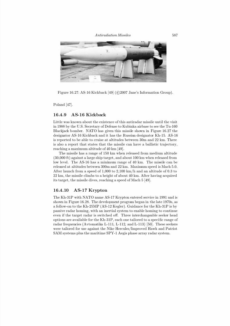
7/17/2019 1596932341 Intercept Radar.pdf
http://slidepdf.com/reader/full/1596932341-intercept-radarpdf 618/891
Antiradiation Missiles 587
Figure 16.27: AS-16 Kickback [49] ( c2007 Jane’s Information Group).
Poland [47].
16.4.9 AS-16 KickbackLittle was known about the existence of this antiradar missile until the visitin 1988 by the U.S. Secretary of Defense to Kubinka airbase to see the Tu-160Blackjack bomber. NATO has given this missile shown in Figure 16.27 thedesignator AS-16 Kickback and it has the Russian designator Kh-15. AS-16is reported to be able to cruise at altitudes between 30m and 22 km. Thereis also a report that states that the missile can have a ballistic trajectory,reaching a maximum altitude of 40 km [49].
The missile has a range of 150 km when released from medium altitude(30,000 ft) against a large ship target, and about 100 km when released fromlow level. The AS-16 has a minimum range of 40 km. The missile can bereleased at altitudes between 300m and 22 km. Maximum speed is Mach 5.0.
After launch from a speed of 1,000 to 2,100 km/h and an altitude of 0.3 to22 km, the missile climbs to a height of about 40 km. After having acquiredits target, the missile dives, reaching a speed of Mach 5 [49].
16.4.10 AS-17 Krypton
The Kh-31P with NATO name AS-17 Krypton entered service in 1991 and isshown in Figure 16.28. The development program began in the late 1970s, asa follow-on to the Kh-25MP (AS-12 Kegler). Guidance for the Kh-31P is bypassive radar homing, with an inertial system to enable homing to continueeven if the target radar is switched off . Three interchangeable seeker headoptions are available for the Kh-31P, each one tailored to a specific range of radar frequencies (Avtomatika L-111, L-112, and L-113) [50]. These seekers
were tailored for use against the Nike Hercules/Improved Hawk and PatriotSAM systems plus the maritime SPY-1 Aegis phase array radar system.

7/17/2019 1596932341 Intercept Radar.pdf
http://slidepdf.com/reader/full/1596932341-intercept-radarpdf 619/891
588 Detecting and Classifying LPI Radar
Figure 16.28: AS-17 Krypton (from [51]).
The Kh-31PM upgrade, now in development, will produce a single inte-grated wideband seeker (L-130, developed by the Avtomatika CKBA plant atOmsk) to replace the L-111, L-112 and the L-113. The MiG-27 Flogger usu-ally carries an APK-8 radar emitter locator pod if equipped with the Kh-31P[50].
The missile has a cruise speed of 700 m/sec and a maximum speed of 1,000 m/sec. The Kh-31 can fly high- or low-level cruise profiles and can belaunched at altitudes of between 100 and 15,000m. Launch speeds range from
600 km/h (Mach 0.65) to 1 m 250 km/h (Mach 1.5). The high-level cruisecan be made at up to 15 km (50,000 ft), with a speed of M3.0. It is reportedthat the Kh-31 missiles can fly at low level, down to 200 m altitude, cruisingat M 2.5 and can maneuver at 10g. The missiles can be programmed to climbat a distance of 2 km from the target, and to dive down onto the target. Themissile is designed to be fired in salvos by one or several launch platforms.
Due to the threat represented by the Kh-31, a unique U.S.-Russian accordwas struck, for the acquisition of missiles by the U.S. Navy for test and trialpurposes. Beginning in 1994, under a joint program with McDonnell Douglas(now Boeing), 13 MA-31 test vehicles were supplied for flight trials. The U.S.has launched its MA-31 targets from QF-4 Phantoms. Follow-on batchesof MA-31 targets have since been delivered but U.S. access to the missilehas now been suspended. In 1998, it was reported that Zvezda-Strela haddeveloped an improved antiradar missile, using the export designation KR-1, with a range increased to 400 km. This missile has been strongly linked

7/17/2019 1596932341 Intercept Radar.pdf
http://slidepdf.com/reader/full/1596932341-intercept-radarpdf 620/891
Antiradiation Missiles 589
with China. Several photographs have now emerged of Kh-31s in Chinesehands. These weapons have appeared in Chinese research facilities and havealso been mounted on a full-scale engineering mock up of the Xian JH-7strike fighter. Chinese sources report that a small numbers of Kh-31Ps havebeen purchased and used as the basis for an indigenously produced variant,the YJ-91. It remains unclear how many Russian-built Kh-31s have beensupplied to China and how many (if any) have been assembled in China.Some sources believe that China has now established its own Kh-31 (YJ-91)production capability [50]. During the 1990s there were reports that an air-to-air version of the Kh-31, designated Kh-31PD, was under development.This was thought to be an antiradiation missile, for use against importanttargets such as AWACS and JSTARS aircraft and others that use airborneearly warning radar.
The Kh-31 has been cleared for carriage on MiG-27 “Flogger,” MiG-29Kand MiG-29SMT “Fulcrum,” Su-17 “Fitter,” Su-24M “Fencer,” Su-25TM
“Frogfoot,” and the Su-30/Su-34 “Flanker” family aircraft. In June 2005 anew upgrade program for the Su-27 to make it compatible with all versionsof the Kh-31 (and other advanced weapons) was revealed and is known asthe Su-27M1. The Kh-31 is also being integrated on Russian air force Su-27sunder the Su-27SM multirole upgrade program [50]. In 2006 an improvedversion of the Kh-31P was under test at Russia’s Akhtubinsk weapons testcenter (the Valery Chkalov State Fight Test Center, or 929 GLITs). Thisweapon was identified as the Kh-31PMK. The designation of the Kh-31PMKmarks it as an export-dedicated program (K, Kommercheskaya, commercial).In practice the K in export programs also stands for China (K, Kitai). TheKh-31PMK is longer than a standard Kh-31P and its range is extended toapproximately 200 km, indicating the incorporation of additional fuel for theramjet. Integration of the Kh-31PMK on the Su-27SM would inevitably make
it available for China, and China’s Su-30MKKs are already operating withthe Kh-31P [50]. Special versions to attack AWACS aircraft such as the E-3ASentry and an antiship version are also available.
16.5 United States
16.5.1 Shrike
After the time of the Korean conflict, the development of radar-guided surface-to-air missiles (SAMs) added a new and lethal threat to U.S. aircraft. Tocombat these new threats, the U.S. Navy started development of an ARM in1958, with the designation ASM-N-10. This missile program would becomethe AGM-45A Shrike, named for the predatory songbird Butcher Bird . TheShrike was based on the airframe of the AIM-7 Sparrow and had a top speedof Mach 2. The Shrike first saw combat in Vietnam in 1966 [4, 8].

7/17/2019 1596932341 Intercept Radar.pdf
http://slidepdf.com/reader/full/1596932341-intercept-radarpdf 621/891
590 Detecting and Classifying LPI Radar
Figure 16.29: Shrike missile AGM-45A (from [52]).
The concept behind the Shrike missile, shown in Figure 16.29 was that
the host aircraft’s radar warning receiver was used to activate the AGM-45’sseeker head that, in turn, notified the pilot (by an audio tone in his headset)that it had achieved a positive lock on the target signal. Following launch,the weapon’s guidance section continuously monitored the threat signal’s di-rection of arrival and generated the appropriate steering commands for themissile’s four mid-body steering surfaces [52]. This enabled the missile tofollow the radar beam down to the emitter and destroy it. This would disablethe SAM site, making it possible to destroy the SAMs themselves or to allowa strike package to pass through the SAM site’s airspace. The first Shrikeswere equipped with seekers optimized for E/F band emitters (2—4 GHz). Asother emitters arose, 10 additional seekers were developed to cover the dif-ferent emitter bands including G-band (4—6 GHz) and I-band (8—10 GHz)[53].
The Shrike first saw combat in Vietnam in 1966. The Shrike was usedby the Wild Weasels to suppress enemy air defense (SEAD). The Shrike hadbetter range than the gravity weapons being used and did not require theaircraft to overfly the SAM sites to identify and destroy them. There werehowever, limitations to employing the Shrike missiles. In order to lock onto the target, the aircraft would have to fly directly at the SAM site. Theaircraft must have had the correct AGM-45 loaded. Also, the maximum oper-ational launch range of the AGM-45A was limited to 16 km but progressivelyincreased to 46 km. Also, SAMs such as the SA-2 had a maximum speed of Mach 3.5 compared to the AGM-45 maximum speed of Mach 2. This wouldallow the SAM site to launch, guide to intercept, and turn off the emitterbefore the AGM-45 could strike the site. Furthermore, the AGM-45 neededto track the emitter until impact. If the emitter shut off , the AGM-45 wouldnot be able to guide to it [37].

7/17/2019 1596932341 Intercept Radar.pdf
http://slidepdf.com/reader/full/1596932341-intercept-radarpdf 622/891
Antiradiation Missiles 591
Figure 16.30: Standard antiradiation missile (from [54]).
16.5.2 Standard ARM
The limited range and warhead of the AGM-45 led to the development of a larger AGM-78 standard ARM as shown in Figure 16.30 [54]. The de-velopment of AGM-78 combined the standard missile airframe (designed forshipboard use) with the Shrike seeker. The standard missile was a radar-guided surface-to-air missile used for ship defense by the Navy. The standardARM had top speed of Mach 2.5, with a maximum range at an altitude of 56km. Due to its size, only two standard ARMs could be carried on an EA-6.The Navy then decided to integrate an improved broadband gimbaled seekerthat allowed the aircrew to avoid flying directly at the target in order to firethe missile. The standard ARM was also able to remember the elevation andazimuth to the target if the emitter shut down. This did not guarantee theemitter would be destroyed since a small amount of drift in the navigationsystem would result in a miss. Although the AGM-78 was an improvement
over the Shrike, its large size limited it to being carried on large aircraft. Inaddition, the standard missile airframe was complicated and costly to operateand maintain.
16.5.3 HARM
The U.S. Navy began development of the AGM-88 high speed antiradar mis-sile (HARM) shown in Figure 16.31 which was light weight allowing it to becarried on U.S. fighters [55]. The top speed is described as over Mach 3. Themaximum range at altitude is 65 miles. The HARM has only one seeker,which uses a broadband antenna to engage the emitters. The features of theHARM are shown in the cutaway view in Figure 16.32 [54]. The HDAM(HARM destruction of enemy air defense attack module) missile variant was
developed partly to address the LPI emitter. It successfully engaged a simu-lated radar system that was radiating at a low power level. The new HDAMvariant adds inertial navigation system/global positioning system (INS/GPS)
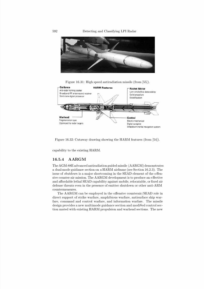
7/17/2019 1596932341 Intercept Radar.pdf
http://slidepdf.com/reader/full/1596932341-intercept-radarpdf 623/891
592 Detecting and Classifying LPI Radar
Figure 16.31: High speed antiradiation missile (from [55]).
Figure 16.32: Cutaway drawing showing the HARM features (from [54]).
capability to the existing HARM.
16.5.4 AARGM
The AGM-88E advanced antiradiation guided missile (AARGM) demonstratesa dual-mode guidance section on a HARM airframe (see Section 16.2.3). Theissue of shutdown is a major shortcoming in the SEAD element of the off en-sive counter-air mission. The AARGM development is to produce an eff ectiveand aff ordable lethal SEAD capability against mobile, relocatable, or fixed airdefense threats even in the presence of emitter shutdown or other anti-ARMcountermeasures.
The AARGM can be employed in the off ensive counterair/SEAD role indirect support of strike warfare, amphibious warfare, antisurface ship war-
fare, command and control warfare, and information warfare. The missiledesign provides a new multimode guidance section and modified control sec-tion mated with existing HARM propulsion and warhead sections. The new

7/17/2019 1596932341 Intercept Radar.pdf
http://slidepdf.com/reader/full/1596932341-intercept-radarpdf 624/891
Antiradiation Missiles 593
guidance section is designed to have a passive antiradiation homing receiverand associated antenna, a GPS/INS, and an active millimeter wave radarfor terminal guidance capability enabling the missile to engage and destroyenemy air defenses in the event that these systems shutdown or employ otherelectronic protection. AARGM is projected to have the capability to transmitterminal data via a weapons impact assessment transmitter to national satel-lites just before AARGM impacts its target. Also incorporated is a provisionto receive off -board targeting information, via the integrated broadcast sys-tem. The AARGM acquisition objective is 1,750 missiles [56]. It will provideUSN and U.S. Marine Corps F/A 18 Hornet and EA-6B Prowler aircrewswith a significantly improved capability to search for, identify, and destroyenemy air defense targets.
16.5.5 Aff ordable Reactive Strike Missile
The aff ordable reactive strike missile (ARES) is a derivative of the AGM-88E advanced antiradiation guided missile (AARGM) under development forthe U.S. Navy and was expected to enter its inventory after 2008 [57]. ARESwould have a range greater than 50 nm and a speed of around Mach 3.0, mak-ing it the “only supersonic, tactical, GPS-guided strike weapon” available.The ARES concept features the same control section going into AARGM andpresents an attractive option for those nations that cannot aff ord to upgradetheir HARMs to the AARGM configuration. Additional options include asemiactive laser seeker for human-in-the-loop control. In missions like pin-point strikes in an urban setting this could allow parts of buildings to betargeted without bringing down the entire structure and injuring civiliansand friendly troops. As with the AARGM, the new control section on ARESwill enable pilots to program exclusion zones in which the missile will not
strike. Aircraft operating the HARM or the AARGM, like the EA-6B, EA-18, F-16, F/A-18, and Tornado, will not require software upgrades to carryARES. The new missile retains the HARM’s rocket motor, airframe and war-head, but adds the new control section and an all-digital passive seeker andmillimeter-wave active terminal seeker to the missile’s front. This allows it toaccurately engage fixed-site and mobile air-defense radars that are emittingor have shut down to avoid detection.
16.5.6 Sidearm
The United States has also developed ARM’s for more defensive roles bytaking advantage of obsolete AIM-9Cs to develop the AGM-122 Sidearm(Sidewinder ARM) as shown in Figure 16.33. The AIM-9C seeker was adapted
to be a broadband passive radar seeker. It also has a gravity bias functionadded to its autopilot in order to facilitate loft launching from low-altitude,low-speed platforms. The AGM-122A was developed for use on Marine he-

7/17/2019 1596932341 Intercept Radar.pdf
http://slidepdf.com/reader/full/1596932341-intercept-radarpdf 625/891
594 Detecting and Classifying LPI Radar
Figure 16.33: Sidearm ARM being loaded onto an aircraft (from [58]).
licopters (Bell AH-1W SuperCobra) to suppress air defense threats. TheAGM-122 was used as a defensive weapon, rather than in an off ensive roleand entered service in 1989 [58]. AGM-122A is noted as having a 10.2 kghigh explosive and fragmentation warhead that is triggered by active laserand impact fusing. Range is given as being approximately 8 km and func-tionally, the weapon alerts the pilot of its host aircraft to lock-on via directionof lock-on symbology on his head-up display and an audio tone in his head-phones [59]. The AGM-122 has a 10-mile range. Once the stock of AIM-9Cswas depleted, the Navy considered building new AGM-122s, but the programnever happened. While Sidearm is less capable than modern antiradiationmissiles (like AGM-88 HARM), it is still a cost-eff ective alternative againstlow-tech threats [60].
16.5.7 Rolling Airframe Missile
The U.S. Navy has developed the rolling airframe missile (RAM) for shipself defense against incoming antiship cruise missiles (ASCMs). The RAM,designated the RIM-116, was a joint venture between the United States andGermany to develop a low-cost self defense system. The RIM-116 shown inFigure 16.34 uses the 5 inch rocket motor and warhead technology from theAIM-9 Sidewinder. The missile is capable of maneuvers up to 20g in any di-rection. The RIM-116 seeker is a dual-mode, passive radio frequency/infraredseeker. Initial guidance is provided by the passive RF seeker on the ASCM’sRF emissions. If the ASCM’s IR radiation is acquired, RAM transitionsto IR guidance. Originally, the missile was cued by the ship’s ES suite or
radar [61].More recently, the RAM has replaced the 20 mm Gatling gun of thePhalanx system. This new marriage of RAM and the Phalanx system is

7/17/2019 1596932341 Intercept Radar.pdf
http://slidepdf.com/reader/full/1596932341-intercept-radarpdf 626/891
Antiradiation Missiles 595
Figure 16.34: Rolling airframe missile launch [61] ( c2007 Jane’s InformationGroup).
called the SeaRAM and combines RAM’s superior accuracy, extended range,and high maneuverability with the Phalanx high resolution radar systems.SeaRAM shown in Figure 16.35, is essentially a Phalanx Block 1B but withthe gun replaced by the 11-cell launcher and is intended to extend ship self-protection to ranges of 4 km and can enable prosecution of low Dopplertargets. In addition to providing an on-mount J-band (12 to 18 GHz), digitalMTI search radar and pulse Doppler monopulse tracker radar, there is also
the electro-optical sensor used in the latest Phalanx systems for surface targetdetection.
16.5.8 Army UAVs
The U.S. Army is exploring potential requirements for an antiradiation mis-sile for carriage by its larger unmanned air vehicles (e.g., AAI RQ-7B Shadow200 UAV) to counter hostile UAV systems [62]. The concept calls for the an-tiradiation missile to target a hostile UAV system’s ground control station byfollowing its command datalink. The option is one of a number of new weaponconcepts being studied by the service as it prepares for the introduction of itsnew General Atomics Sky Warrior and Northrop Grumman RQ-8B Fire ScoutUAVs. The development of an anti-UAV capability anticipates that UAV sys-
tems will continue to be an important operational target. Strategies such astargeting unmanned aircraft to take away the intelligence, surveillance and

7/17/2019 1596932341 Intercept Radar.pdf
http://slidepdf.com/reader/full/1596932341-intercept-radarpdf 627/891
596 Detecting and Classifying LPI Radar
Figure 16.35: SeaRAM missile launch [61] ( c2007 Jane’s InformationGroup).
reconnaissance capability is a significant tactical response. Other anti-UAVcapabilities being studied include the use of electronic warfare techniques suchas countertargeting and jamming of the command datalink.
16.6 France
The French introduced the Armat (Anti-Radar Matra) in 1984 which was anevolved variant of the antiradiation version of the French-British BAe-MatraAS-37 Martel missile. By using the AS-37 airframe and replacing the seekerand associated electronics with new and improved versions with added elec-tronic protection, the missile shown in Figure 16.36 was given the capabilityto overcome decoys and jamming techniques including long radar switch-off periods. The microprocessor based seeker homes on to a programmed emitterand uses inertial midcourse guidance. Several interchangeable homing headsare used to cover the wide spectrum of target radar frequencies including L-band (500—2,000 MHz), S-band (2—4 GHz), C-band (4—8 GHz) and X-band(8—12 GHz) [63]. The missile can be launched from high or low levels andwill home onto the radar or jamming transmissions of the pre-selected targetradar. After lock-on of the missile seeker, the location, radar parameters and
launch success zones are displayed to the aircrew who can then select thebest launch time. With its high launch weight, heavyweight warhead andlong range, the Armat is primarily an off ensive strategic ARM designed to

7/17/2019 1596932341 Intercept Radar.pdf
http://slidepdf.com/reader/full/1596932341-intercept-radarpdf 628/891
Antiradiation Missiles 597
Figure 16.36: AS-37 Martel.
destroy early warning and ground control intercept radars. This is where itdiff ers fundamentally from the HARM and the ALARM, which are built to
also perform as defensive ARMs carried as part of a mixed weapon load. Themissile has been cleared for carriage on Jaguar, Atlantique, Mirage F1, Mi-rage III and Mirage 2000 aircraft. The missile is believed to have a maximumrange of 100 km when launched from high altitude. An improved version hasalso been produced, the Armat-D, which is fitted with an updated passivehoming seeker.
16.7 United Kingdom
In the early 1980s, the British conducted a study to replace their aging AS-37s. The British decided on the Alarm for several reasons. The UnitedStates developed HARMs for specially equipped aircraft, such as the F-4G
Wild Weasel and the EA-6. Both of these aircraft are equipped with sophisti-cated and complex emitter locating systems. Since the British have a smallernumber of aircraft than the U.S., they did not want to limit the role of anyaircraft by specially equipping them. With the smaller numbers, the Britishrequired that all of their fighters be able to conduct any mission. The Britishalso did not wish to incur the cost and in-service support overheads of deploy-ing and maintaining these sophisticated and complex systems. Additionally,the British thought that adopting the Weasel operational model would exposeSEAD aircraft to attack more frequently, thus incurring high loss rates. TheAlarm can be carried on all British fighters, such as the Harrier and Tornado,which carry up to nine Alarms. Figure 16.37 shows the launch of an Alarmfrom a Tornado [63].
The Alarm has a range of 28 miles and has five launch modes: direct,
dual, loiter, universal, and area suppression. A unique feature to the Alarmis it parachute system for loitering over the target area. In the dual andloiter modes, the missile climbs to a high altitude above the target area and

7/17/2019 1596932341 Intercept Radar.pdf
http://slidepdf.com/reader/full/1596932341-intercept-radarpdf 629/891
598 Detecting and Classifying LPI Radar
Figure 16.37: Alarm missile firing from an RAF Tornado (from [63]).
searches for the enemy emitter. If one is detected, the missile dives on thetarget. If not, it deploys a parachute and listens for the enemy emitter to
come up. Once the radiation is detected, the missile jettisons the chute anddives on to the emitter. The parachute system allows the ALARM to loiterfor several minutes. With ALARM-equipped aircraft in the area, enemy SAMsites would not know when it was safe to turn on their radars, thus suppressingtheir ability to deter attacking aircraft.
Figure 16.38 shows the modes used by the Alarm. The Alarm’s seeker issimilar to that of the HARM with a microprocessor controlled passive homingreceiver, designed to locate and identify the characteristic Pulse RepetitionFrequencies (PRF) of programmed threat emitters [63]. The Alarm has awideband RF antenna/receiver and a conventional quartet of cavity backedspiral antennas, forming a fixed two axis interferometer with lower mid-bandto hi-band coverage. Like the HARM, the Alarm has logic to select the highestvalue alternate target, should the primary target go off the air.
16.8 Taiwan
Taiwan is intensely concerned about China’s growing air power dominanceof the Taiwan straits. Having an eff ective ARM capability hinders China’sability to conduct air operations from secure bases on the mainland. Sinceno country will export ARMs to Taiwan, its air force has developed its ownARM, known as the Tien Chien IIA. Tien Chien translates to “sky sword.”The Tien Chien IIA replaces the active radar seeker of the Tien Chien IIair-to-air missile with a passive antiradar seeker and guidance section. Theseeker is housed in a reprofiled, notched fairing, giving rise to speculation thatit may use a dual-mode design, incorporating both passive RF and infrared
sensors [64].The Tien Chien IIA equips the Republic of China’s Air Force’s AIDC F-
CK-1 Ching Kuos (otherwise known as the IDF, Indigenous Defense Fighter).

7/17/2019 1596932341 Intercept Radar.pdf
http://slidepdf.com/reader/full/1596932341-intercept-radarpdf 630/891
Antiradiation Missiles 599
Figure 16.38: Alarm modes of attack (from [63]).
Figure 16.39: Tien Chien 11A being carried by an indigenous defense fi
ghter.
According to the Chung-Shan Institute of Science and Technology (CSIST),any Ching Kuo can carry the new ARM, as it requires no modifications tothe launch aircraft. The ROCAF does not intend to field a dedicated “WildWeasel” defense suppression force armed with the Tien Chien IIA. Instead,the capability will be introduced across the front-line fleet. Up to four TienChien IIAs can be carried by one aircraft on individual pylons—without losingthe existing hardpoints for two Tien Chien IIs plus two wingtip-mounted TienChien Is. Tien Chien IIA can be carried on any aircraft equipped to carrythe Tien Chien II as shown in Figure 16.39.

7/17/2019 1596932341 Intercept Radar.pdf
http://slidepdf.com/reader/full/1596932341-intercept-radarpdf 631/891
600 Detecting and Classifying LPI Radar
Figure 16.40: German ARMIGER [65] ( c2007 Jane’s Information Group).
16.9 Germany
Germany, a longtime user of the HARM, is developing the ARMIGER (antira-diation missile with intelligent guidance and extended range). The Germanshave been participating in the development of the international HARM up-grade program, the AGM-88D. The improvements consist of software andhardware upgrades including replacing the original mechanical gyros with astate-of-the-art GPS/IMU. The addition of GPS to the HARM would correctthe long-standing problem of ARMs of what to guide on if the emitter shutsdown. GPS allows you to fly to a certain point when the target is not emittingat all. However, the U.S. Navy decided not to proceed with the project. TheGermans decided to proceed with the ARMIGER program as a replacementfor the HARM. Due to concerns over whether it is wise to develop a singlepurpose weapon, the German Luftwaff e has decided to proceed slowly withthe ARMIGER [65].
The ARMIGER is roughly the same weight as the HARM. The ARMIGERwill have a GPS/IMU, as would the AGM-88D, to overcome the ARMproblem when the emitter shuts down. In addition to the GPS/IMU, theARMIGER will have a new technology passive radar/high-resolution imag-ing infrared dual-mode seeker (called ARAS). This dual-mode seeker will alsocombat the problem of an emitter shutting down while the missile is in flight.Typically, the ARMIGER would be launched using the passive radar andswitch over to the infrared for terminal tracking if the targeted emitter shutsdown. In addition to the seeker, the ARMIGER will have improved rangeover the HARM. The GPS will bridge the gap between the time when thepassive radar seeker loses track of the radar emitter and the point when theenemy radar is detected by infrared. Combined GPS information collectedby multiple aircraft can be used to find the position of enemy radar with the
information then passed to the ARM prior to its launch from the aircraft [65].

7/17/2019 1596932341 Intercept Radar.pdf
http://slidepdf.com/reader/full/1596932341-intercept-radarpdf 632/891
Antiradiation Missiles 601
16.10 Israel
16.10.1 Harpy
Dedicated for the SEAD mission, Harpy is an operational loitering attackweapon. The current version of Harpy is deployed as a fire and forget weapon.In order to verify the drones operational capability, its seeker head is beingtested by a special radar simulator just before launch, to ensure that all sys-tems are working. It patrols the assigned area, and will attack any hostileradar activated in its vicinity. When used in appropriate numbers, Harpycan be launched into a target area to support continuous operations, or timelimited strike packages. Unlike antiradar missiles such as HARM, whosespeed, range and direction of approach are predictable, the killer-drone de-ployment is more flexible and unpredictable, and therefore, conventional coun-termeasure techniques are not useful against it. The Harpy system shown inFigure 16.41 is designed to operate multiple munitions simultaneously over
a specific area, to eff ectively cover the target. Each drone is deployed au-
Figure 16.41: Harpy antiradar UAV being launched from a truck canister [66]( c2007 Jane’s Information Group).
tonomously, without interference and overlapping the other drones [66].The Harpy mission is planned and programmed in the ground control cen-
ter, as an independent mission, or planned in accordance with other mannedor unmanned systems. Prior to launch, individual weapons are programmed
and tested, to verify their operational readiness. After the rocket-assistedlaunch, the drone flies autonomously in route to its patrol area, predefinedby a set of navigational waypoints. Due to its low speed and economical fuel

7/17/2019 1596932341 Intercept Radar.pdf
http://slidepdf.com/reader/full/1596932341-intercept-radarpdf 633/891
602 Detecting and Classifying LPI Radar
consumption, the drone can sustain a mission of several hours over the targetarea. Its radar seeker head constantly searches for hostile radars. Once anenemy radar is acquired, Harpy compares the signal to the library of hostileemitters, and prioritizes the threat. If the target is verified, the drone entersan attack mode and a near vertical dive homing in on the signal. The attacksequence is shown in Figure 16.42. The drone is set to detonate its warhead
Figure 16.42: Harpy UAV attack sequence against an emitter [66] ( c2007Jane’s Information Group).
just above the target, to generate the highest damage to the antenna, and sur-rounding facilities. If the radar is turned off before Harpy strikes, the dronecan abort the attack and continue loitering. If no radar was spotted duringthe mission, the drone is programmed to self-destruct over a designated area.
Follow-on systems are calling for a combination of seeker and killer dronesthat will enable visual identification and attack of targets even after they turnoff their emitters.
Current Harpy canisters are installed on trucks, and can be carried by C-130 transport aircraft. Each truck carries 18 weapon launchers. Each batteryof Harpy is composed of three trucks, capable of deploying up to 54 dronesfor simultaneous, coordinated attack . The battery also has a ground controlstation and logistical support element. The system can also be deployedfrom the decks of assault landing ships, in support of marine or amphibiousoperations. Harpy is currently operational with the Turkish, Korean, Chineseand Indian Armies, in addition to the Israel Air Force. In December 2004China was reported to be interested in an upgrade of its systems to a moreadvanced version.

7/17/2019 1596932341 Intercept Radar.pdf
http://slidepdf.com/reader/full/1596932341-intercept-radarpdf 634/891
Antiradiation Missiles 603
Figure 16.43: STAR-1 antiradiation missile [67] ( c2005 Jane’s InformationGroup).
16.10.2 STAR-1
Israel Military Industries (IMI)–formerly TAAS–has developed its Delilahair-launched decoy into a long-range, lightweight cruise missile. Describedby its manufacturer as an advanced air-to-ground standoff powered UAV,the Delilah has a range capability that takes it out of the tactical categoryand into the realms of the cruise missile. Furthermore, the official maximumrange quoted for the system is 250 km. The original Delilah decoy was derivedfrom the US MQM-74 Chukar aerial target, that entered service in the mid-1960s. The first reports that Israel had developed the Delilah air vehicle asan off ensive weapons system emerged in 1995 [67]. Since then, the Delilah hasevolved into a modular air strike weapon with a range of possible applications.Driving the design of the Delilah system was an emphasis on single-pilotoperations. The weapon is programmed on the ground with key parameters
such as waypoints and fl
ight altitudes, but a datalink gives the launch aircraftthe ability to retask the missile in flight. During the mid-1990s a long-rangeantiradar defense suppression variant of the Delilah was actively marketedunder the designation STAR-1. This program was linked with China in severalreports but has since disappeared from view and is no longer included in IMI’sofficial product portfolio. To give the Delilah a SEAD capability, a broadband,2—18-GHz, passive radar seeker with an INS/GPS mid-course update systemwas incorporated into its basic design. The STAR-1 shared the same size andweight of the Delilah, and used the standard 30 kg warhead. The STAR-1 asshown in Figure 16.43, would have both a direct attack mode and the abilityto loiter over a target area waiting for hostile radars to start transmitting, orto reattack radars if they restart transmissions after an attack. A STAR-1variant (or equivalent) is believed to be in service in Israel and was off ered
for export as far back as 1995. In 2004 an IMI representative said that adual-mode antiradiation seeker was available for the Delilah, but that it wasnot being off ered as a product yet. It is understood that the STAR-1 can be

7/17/2019 1596932341 Intercept Radar.pdf
http://slidepdf.com/reader/full/1596932341-intercept-radarpdf 635/891
604 Detecting and Classifying LPI Radar
both air-launched and ground-launched [67].IMI has now developed several versions of the Delilah, which can be
launched from land, sea and air. The standard Delilah missile can be fit-ted with interchangeable FLIR (forward looking infrared) or electro-opticalseekers, in separate seeker assemblies. The seekers have a target auto-trackingcapability but not yet an automatic target recognition function. In tests theDelilah has proved its ability to hit a target moving at 50 km/h, and IMIis promoting the system for use against time-critical targets such as mobileSSMs or SAMs. The existing seekers are capable of identifying targets atranges of up to 10 miles. Operators have found that moving targets areeasier to locate and identify than static ones. The missile’s datalink capa-bility allows for man-in-the loop control, to confirm the final target. If thistarget is not confirmed, or if datalink communications are lost, the missilehas a default navigation mode to fly around the target and reengage. TheDelilah carries enough onboard fuel to fly for a maximum of 22 minutes, so
the weapon is optimized for high-altitude straight line cruise profi
les. A 30-kghigh explosive warhead is currently fitted, but IMI confirms it is working ona new penetrating warhead option for hardened target attacks [67].
16.11 China
The China National Precision Machinery Import and Export Corporation(CNPMIEC) off ers the FT-2000 (Chinese Fei Tung = FT), which is an ex-port variant of the antiradar surface-to-air system specifically for use againstairborne early warning, command and control, and EA aircraft. It is believedthat the missile is an upgrade of the SA-10 design. The missile system has theChinese designator Hong-Qi-12 (HQ-12)[68]. The missile contains a widebandsurface-to-air passive seeker to engage either single or multiple radiating air-borne targets that radiate in the 2—18 GHz band such as the Airborne EarlyWarning and Command System (AWACS) or Suppression of Enemy Air De-fense (SEAD) EA-6B/EA-18G EA aircraft. The missiles are also capable of detecting and locking on to random electronic interference and jamming.
With primarily Russian technology and with minimal use of importedcomponents, China has mastered the production of air defense missile systemssuch as the HQ-15 missile. This missile is shown in Figure 16.44 along withits transporter-erector launcher vehicle. A photograph of the passive radarseeker assembly for the HQ-15 missile is shown in Figure 16.45. A typicalHQ-12 battalion has three batteries. Each battery has four ES vehicles, threetransporter erector launchers (TELs), one command launch center, and threetransporter/loader vehicles. The ARMs are vertically cold launched from the
TEL Taian TAS5380 that is also an 8 × 8 transport vehicle as shown in Figure16.45. The TEL has four missile canisters that are raised to the vertical forlaunching. The four ES stations are deployed at distances of up to 30 km in a

7/17/2019 1596932341 Intercept Radar.pdf
http://slidepdf.com/reader/full/1596932341-intercept-radarpdf 636/891
Antiradiation Missiles 605
Figure 16.44: Outline drawing and launch system for the Chinese HQ-15missile.
Figure 16.45: Photograph of the passive radar seeker assembly for the ChineseHQ-15 missile.
7/17/2019 1596932341 Intercept Radar.pdf
http://slidepdf.com/reader/full/1596932341-intercept-radarpdf 637/891
606 Detecting and Classifying LPI Radar
triangle with a central fourth unit acting as command and control. The fourES receiver vehicles associated with each battery can track up to 50 targets.The complete FT-2000 system includes a wideband passive radar detectingstation, the specially developed ARM vertically launched missile and a four-round launcher platform. A first test launch was reported in September 1997.The passive seeker has a memory, for use if the target radar is switched off ,and a home-on-jam capability. The missile has a maximum speed of 1.2 km/s.Targets can be intercepted at altitudes between 3 and 20 km. The proximityfuse is activated 5 km from the target with a range of 35m.
The second version, known as FT-2000A in its export version, was re-ported to have a passive radar seeker covering the 2—6-GHz (S and C-band)range, that has its frequency selected on the ground before launch. This mis-sile has a maximum range of 60 km, and can be used as part of the HQ-2system but requires separate launchers and fire-control units. This system isstill in the developmental stages but is expected to be a static weapon system
[69]. The FT-2000B version has been designed for use as an upgrade to theHQ-12 missile system, with the maximum range increased to 120 km and witha new 1—18-GHz passive radar seeker. The system has been off ered for exportwith the potential first customer Pakistan. During discussions between Chinaand Pakistan in February 2004, the off er was made by China to supply theFT-2000/FT-2000A to counter the Indian threat to Pakistan of the IndianAgni missile systems. Batteries have been reported around Beijing and inFujian province.
16.12 Anti-ARM Techniques
The earliest form used to defeat the ARM (and still the most commonmethod) is radar position fl exibility . In most cases the radar position be-ing attacked is provided by an electronic intelligence (ELINT) system priorto aircraft takeoff . The ability of the radar to set up, tear down, and moveto a new location within a few minutes can help to hide the radar position.The latest generation of SAMs have put a much higher premium on systemmobility. That is, the ability to leave in a hurry is closely linked to survivalin modern warfare. Most land-based surveillance, ballistic missile detectionand weapon-related radars currently in development claim to have relativelyhigh mobility, including some of the very powerful long range systems such asMarconi’s latest version of Martello, the S 753, and the Israeli Arrow GreenPine antiballistic missile radar.
Rapid relocation however, has its limits. If a surveillance radar is attackedby an ARM fired from below the radar horizon, or by an aircraft approaching
low over the horizon, the radar has approximately 20 seconds to move to asafe location. Consequently, manufacturers are looking to increase mobility,with multifunction radars using planar-array antennas, mounted on a truck
7/17/2019 1596932341 Intercept Radar.pdf
http://slidepdf.com/reader/full/1596932341-intercept-radarpdf 638/891
Antiradiation Missiles 607
(including all of the electronics), and with a microwave link to relay targetdata back to command and control. They will also use highly sophisticatedland navigation systems to provide an accurate position reference. This isimportant if their target data is to be tied into an overall battlefield awareness.
Radar methods include twinkle (or blink) transmission. In this technique,the off time is much greater than the on time. This makes it difficult for theARM to keep track of the emitter’s signal (and location). In this methodof protecting a pulse radar from an ARM missile attempting to home inon interrogating pulses emitted, a number of decoys at diff erent locations aredeployed in the vicinity of the pulse radar. Each one of the decoys are adapted,when activated, to emit pulses of a given amplitude and duration; activating,when each one of the interrogating pulses is generated in the pulse radar. Aselected decoy is chosen to lead the remaining decoys for a period of timedetermined by range and range rate measurements of a pulse Doppler missilewarning sensor. The decoy selected is changed to lead the remaining decoys
at a time determined from the range and range rate measurements of a pulseDoppler missile warning sensor thereby defining a blink rate associated withthe decoys, to form a covering pulse overlapping the then emitted one of theinterrogating pulses, and adaptively changing the blink rate. Two examplesof radar using this transmission control technique for anti-ARM include theAN/APY-1 Cosmic Shield and the AN/MPQ-53 Patriot [70].
Another technique often used is called the snap-and-shoot method. In thistechnique, a fire control radar is assigned to intercept and track targets. Theremaining fire control radar systems receive the target flight path parameters.When the tracked targets enter the fire range, the unit snaps open and makesthe response. Other methods that may be used include using other typesof radiation to detect and track the targets. This may include using visualtelevision with infrared measurements of the target’s range. Examples of this
include the Swedish GLV200 and the Swiss Air Guard. Also, the use of veryhigh frequency (VHF) band or ultra high frequency (UHF) bands can be usedto avoid the ARM attack [70]. The reason for this is that the diameter of theARM body is limited with the aperture of the ARM antenna greater than thewavelength. For example, with a diameter of 40 cm, it is difficult to targetradar with frequencies below 1 GHz.
16.12.1 Decoys
Dispensing of active decoys is also an important method for anti-ARM [71].The ARM decoy has characteristics that are coincident with the radar. Forexample, the decoy has the same eff ective radiated power (or ERP) and carrierfrequency and the transmission waveform is synchronous with the radar. The
decoy also emits a decoy pulse 0.1—0.2 μs ahead of the radar pulse so that theARM triggers its guidance on the wrong waveform. Typically, the distancebetween the radar and the decoy is 100—300m with the spatial angle between
7/17/2019 1596932341 Intercept Radar.pdf
http://slidepdf.com/reader/full/1596932341-intercept-radarpdf 639/891
608 Detecting and Classifying LPI Radar
Figure 16.46: Flaps technology for decoying an ARM (from [72]).
radar and decoy smaller than the ARM track angle resolution.An ARM decoy antenna that uses low-windload FLAPS (flat parabolic
surface) technology is shown in Figure 16.46 [72]. Once the incoming ARM isdetected, the radar is turned off and the reflectors are illuminated by a remotefeed. Since the frame is staked to the ground, it can survive an ARM blastfrom any direction. The blast travels through the aperture then the reflectorsprings back to is operating position. The antenna uses FLAPS technologyto enable a geometrically flat surface as shown in Figure 16.47(a) to behave
electromagnetically as though it were a parabolic reflector as shown in Fig-ure 16.47(b). The FLAPS reflector is a thin (planar or conformal) surfaceconsisting of an array of dipole scatterers. The elemental dipole scatterer asshown in Figure 16.47(c), consists of a dipole positioned approximately 1/8wavelength above a ground plane. Here, a crossed shorted dipole configu-ration is shown with each dipole controlling its corresponding polarization.Incident RF energy causes a standing wave to be set up between the dipoleand the ground-plane [72]. The dipole itself possesses an RF reactance whichis a function of its length and thickness. This combination of standing-waveand dipole reactance causes the incident RF to be reradiated with a phaseshift, which can be controlled by a variation of the dipole’s length [72].
The integrated ARM warning radar and decoy deployment method is shownin Figure 16.48 and consists of an integrated system of advanced ARM de-tection radar and general purpose distributed decoys to protect the groundair-defense radar [73]. The ARM detection radar is used to detect and iden-

7/17/2019 1596932341 Intercept Radar.pdf
http://slidepdf.com/reader/full/1596932341-intercept-radarpdf 640/891
Antiradiation Missiles 609
Figure 16.47: FLAPS antenna technology showing (a) a thin planar surfaceconsisting of an array of radiating and phase shifting elements, (b) a conven-tional reflector, and (c) the schematic of an elemental dipole scatterer usedin the FLAPS antenna technology (from [72]).
tify the attacking ARM (RCS = 0.1 m2), which triggers a shutdown of thesensors and cues the crew manning the site to leave. Studies also indicatethat by using changeable sample ratios within the radar receiver, a higherprobability of ARM detection can result [74].
ARM detection radars with multiple antennas using VHF have also beenreported [75]. The use of VHF enhances the ARM RCS significantly increas-ing the probability of detection. Extended coherent integration and dedicatedsignal processing can also be used. At the same time, the ARM messages aresent to a series of decoys. The signal radiated by the decoys guide the ARM(speed 2 to 4 Mach) to a preset safety area. If the ARM fails to continuethe attack, a cancellation of the alarm is made and protected radar triggeredto restart. The anti-ARM warning radar’s frequency band selection (UHF,VHF) is to give an antistealth capability, ground clutter and weather sup-pression and to also control the deployment of the decoys. It must be highlymobile to operate in the sometimes rough terrain and also have good targetidentification capability. The PRF of the warning radar should be as large aspossible with a compressed pulse width as small as possible to decrease theenergy in the range-Doppler detection cell.
With high-speed ARM detection (>1.5 Mach), the separation of the mis-sile from the launch aircraft can be detected with the warning radar usingpulse-Doppler waveforms and frequency agility [73]. For slow ARM targetssuch as UAV ARMs and cruise ARMs, an accurate radial velocity and unam-
biguous range of the target must also be reported.To avoid turning the radar off early and deploying the decoys, two trans-mitters T1 and T2 can be used that are placed far away from the protected

7/17/2019 1596932341 Intercept Radar.pdf
http://slidepdf.com/reader/full/1596932341-intercept-radarpdf 641/891
610 Detecting and Classifying LPI Radar
Figure 16.48: Deployment of the integrated anti-ARM system (adapted from[73]).
radar with the receiver placed near the protected target as shown in Fig-ure 16.48. They should be connected by an RF optical fiber communicationlink. When the ARM approaches, T1 and T2 can work together to protecteach other. Their use of polarization and frequency diversity can provide themeans to reduce the power of each solid state transmitter by 3—5 dB. Thetwo transmitters are noncoherent and can be placed at diff erent heights toprevent lobe splitting [73]. The antenna should be a small foldable, nonrota-tion antenna array. Because the distance between T1 and T2 and the receivercannot be too far, the use of othogonal waveforms such as those discussed in
Chapter 10 are required.Another type of decoy is the simulated model—in eff ect, a cardboard cut-
out that looks like a radar. These can be very eff ective, and it is possibleto metalize them to provide a radar return that looks like a gun, a tank, ora radar station. This type of decoy has been used very eff ectively againstground attack aircraft threats, and could contribute toward the protectionfrom the active radar homing phase in a dual-mode ARM.
16.12.2 Gazetchik
The Iraqi newspaper Al-Qabas Daily , in July 2000, reported that Iraq hadacquired from Russia a jamming device that was capable of neutralizing U.S.ARMs during the enforcement of the no-fly zones, making the missiles miss
their targets. The first two systems were reported to be a gift to Baghdadby the Russian ultra-nationalist leader Vladimir Zhirinovsky. The Gazetchikanti-ARM system built by the All-Russian Radio Engineering Research Insti-

7/17/2019 1596932341 Intercept Radar.pdf
http://slidepdf.com/reader/full/1596932341-intercept-radarpdf 642/891
Antiradiation Missiles 611
Figure 16.49: Russian Gazetchik anti-ARM system.
tute, Moscow, is designed to protect radar emitters such as the GAMMA-DE(67N6E) (a mobile 3-D solid-state phased array surveillance radar) from at-tack by ARMs.
The Gazetchik system shown in Figure 16.49 consists of a stand-alonedetector, active radio frequency decoys, a set of passive countermeasure dis-persers (not shown), and an interface with the radar or radars being defended.The ARM detector unit alerts the system to the approach of an incomingARM weapon. Then a warning is initiated that activates a host of responsesincluding interruption of the protected emitter’s transmission, transmissionof RF decoy signals on the protected emitters operating frequency and the
firing of passive decoys from the equipment’s chaff and aerosol launchers [75].With coverage of up to 90 degrees elevation and 360 degrees azimuth, thesystem operates autonomously and draws its power from the radar systemsbeing protected. Gazetchik is reported to be available in a number of variantsand has an automatic operating mode if required.
16.12.3 AN/TLQ-32 ARM-D Decoy
AN/TLQ-32 ARM-D is a lightweight, ruggedized, tunable magnetron thatimitates the AN/TPS-43E and AN/TPS-75 radar signals. It is designed toprotect radars in the field from ARMs that are guided by homing in onthe radar’s own transmission signals. The ARM-D built by ITT Gilfillan,provides protection to the radar by emulating the transmission characteristics
of the host radar, thereby deceiving and confusing the incoming missile. Thedecoys are placed on the ground as shown in Figure 16.50 in triangulationto attract enemy antiradiation missiles, and ultimately saving the radar site.

7/17/2019 1596932341 Intercept Radar.pdf
http://slidepdf.com/reader/full/1596932341-intercept-radarpdf 643/891
612 Detecting and Classifying LPI Radar
Figure 16.50: AN/TLQ-32 anti-ARM radar transmitter [76] ( c2004 Jane’sInformation Group).
Features of ARM-D include its capability to emulate frequency-agile radars;360o coverage; protection of both the radar and the decoy assets againstARMs; lightweight fiber optic interface between the radar and decoy emittergroups and low prime power operation. It also features rugged, lightweightmodular packaging, extensive built-in test capability and rapid set up andtear down. It is claimed that the decoy can be transported by two peoplewith individual decoys being deployable within 15 minutes. In operationaluse, three decoys are allocated to each radar system. The surveillance decoysare designed to be capable of protecting the radar site from multiple missilelaunches, whether simultaneous or consecutive [76].
The AN/TLQ-32 ARM-D was selected by the USAF in March 1989, witha contract for two “first article” examples being awarded during the followingSeptember. Testing of these began in May 1992 and full-scale production of
14 systems to protect USAF AN/TPS-75 radars began in December 1992.During 1996, additional TLQ-32 systems were delivered to the U.S. Air Na-tional Guard.
References[1] Bolkcom, B., “Military suppression of enemy air defenses (SEAD): Assessing
future needs,” CRS Report for Congress, RS21141, Sept. 23, 2004.
[2] Farroth, A., and Krishnamurthy, V., “Optimal threshold policies for hard-kill of enemy radars with high-speed anti-radiation missiles (HARMs),” Proc.of the International Conference on Acoustics, Speech and Signal Processing ,14-19 May, 2006.
[3] Department of the Army, Field Manual 101-5: Sta ff organization and opera-
tions, May 1997.[4] Davis, L., Wild Weasel: The SAM Suppression Story—Vietnam, Squadron
Signal Publications, July 1993.

7/17/2019 1596932341 Intercept Radar.pdf
http://slidepdf.com/reader/full/1596932341-intercept-radarpdf 644/891
Antiradiation Missiles 613
[5] Friedman, N., US Naval Weapons, Conway Maritime Press, 1983.
[6] Parsch, A., “Corvus,” Encyclopedia Astronautica,
www.astronautix.com/lvs/corvus.htm[7] Gunston, B., The Illustrated Encyclopedia of Rockets and Missiles, Salaman-
der Books Ltd, 1979.
[8] Streetly, M., Airborne Electronic Warfare: History, Weapons and Tactics,Jane’s Information Group, 1988.
[9] Pietrucha, M., “Starbaby”: “A quick primer on SEAD,” Defense IQ AirborneElectronic Warfare Conference, London, England, Aug. 2006.
[10] Levin, R. E., “Electronic Warfare—Comprehensive strategy needed for sup-pressing enemy air defenses,” United States General Accounting Office Reportto Congressional Requesters, GAO-01-28, Jan. 2001.
[11] Kopp, C., “Support jamming and force structure,” The Journal of Electronic Defense, May, 2002.
[12] Lum, Z., “Hardcore Hard Kill: Seeds of a New SEAD,” Journal of Electronic Defense, February 1997.
[13] McKenna, T., “Poisoned Arrows,” The Journal of Electronic Defense , March2004.
[14] Zaloga, S. J., “The evolving SAM threat: Kosovo and beyond,” The Journal of Electronic Defense, May, 2000.
[15] Lambeth, B. S., “Kosovo and the continuing SEAD challenge,” Air Power Journal, Summer 2002.
[16] Martin, N. M., Nandagopal, D., Kara, M., Tran, V. N., and Hamilton, S.“Body fixed antenna options for seekers,” Proc. of the IEEE International Conference on Radar , pp. 272—275, Oct. 1992.
[17] Cencich, T. and Huff man, J., “The analysis of wideband spiral antennas using
modal decomposition,” IEEE Antennas and Propagation Magazine, Vol. 46,No. 4, Aug. 2004.
[18] Muller, D. J., and Sarabandi, K., “Design and analysis of a 3-arm spiralantenna,” IEEE Trans. on Antennas and Propagation, Vol. 55, No. 2, pp.258—266, Feb. 2007.
[19] Mayes, P. E., “Frequency-independent antennas and broad-band derivativesthereof,” Proc. of the IEEE , Vol. 80, No. 1, pp. 103—112, Jan. 1992.
[20] Thaysen, J., Jakobsen, K. B., and Appel-Hansen, J., “A logarithmic spiralantenna for 0.4 to 3.8 GHz,” Applied Microwaves & Wireless pp. 32—45, 2001.
[21] Stutzman, W. L., and Thiele, G. A., Antenna Theory and Design , John Wiley& Sons, Inc. New York, 1997.
[22] Balanis, C. A., Antenna Theory Analysis and Design , Harper & Row, Pub-
lishers, New York, 1982.[23] Salmond, W. E., “High accuracy broadband antenna system,” U.S. Patent
4,095,230, June 13, 1978.

7/17/2019 1596932341 Intercept Radar.pdf
http://slidepdf.com/reader/full/1596932341-intercept-radarpdf 645/891
614 Detecting and Classifying LPI Radar
[24] Salmond, W. E., “Common aperture dual mode seeker antenna,” U.S. Patent4,348,677, Sept. 7, 1982.
[25] Corzine, R. G., Bolstad, B. E., and Johantgen, J. S., “Broadband polarizationdiversity monopulse antenna,” U.S. Patent 5,021,796, June 4, 1991.
[26] Bohlman, W. A., and Schuchardt, J. M., “Dual polarized ambidextrous mul-tiple deformed aperture spiral antennas,” U.S. Patent 5,227,807, July 13,1993.
[27] Neri, F., Introduction to Electronic Defense Systems, 2nd ed., Artech House,2001.
[28] Hughes, R. S., “RF detector logarithmic video amplifier,” Microwave Journal ,vol. 32, no. 8, pp. 137—148, Aug. 1989.
[29] Jane’s Information Group, “Two-for-one guidance could steer future anti-radar missiles,” Jane’s Missiles and Rockets , Jan. 2005.
[30] Klass, P. J., “New anti-radar missile uses dual-mode seeker,” Aviation Week and Space Technology , pp.60 Oct., 26 1998.
[31] Penz, P. A., Katz, A., Gately M. T., Collins, D. R., and Anderson J. A.,“Analog capabilities of the BSB model as applied to the anti-radiation homingmissile problem,” IEEE Conference, pp. II-7 — II-11.
[32] Lee, J. P. Y., “Circuit for LPI signal detection and suppression of conventionalpulsed signals,” U.S. Patent 6,388,604, issued May 14, 2002.
[33] Shirman, Y. D., Orlenko, V. M., and Seleznev, S. V., “Passive detection of the stealth signals,” Proc. of the European Radar Conf., Amsterdam, pp.321—324, 2004.
[34] Shirman, Y. D., Orlenko, V. M., and Seleznev, S. V., “Present state and waysof passive anti-LPI radar implementation,” Proc. of the International Radar Symposium , pp. 1—4, 24-26 May, 2006.
[35] Jie, S., Xiao-ming, T. and You, H., “Multi-channel digital LPI signal detec-
tor,” Proc. of the International Conf. on Radar , pp. 1—4, Oct. 2006.
[36] Kopp, C. “Texas Instruments (Raytheon) AGM-88 HARM,” Air Power In-ternational , Vol. 4, No. 1, Dec. 1998.
[37] Fiszer, M. and Gruzczynski, J., ”Crimson SEAD,” The Journal of Electronic Defense , pp. 44 — 56, Oct. 2001.
[38] Barrie, D., “Silent Hunter,” Aviation Week and Space Technology, pp. 36,July 26, 2004.
[39] http://www.fas.org/man/dod-101/sf/missile/row/aa-10.htm
[40] http://www.fas.org/nuke/guide/russia/bomber/as-4.htm
[41] Jane’s Strategic Weapon Systems, “Kh-22 (AS-4 ’Kitchen’/Burya)”, Sept.2007.
[42] Jane’s Strategic Weapon Systems, “KSR-2P (AS-5 ’Kelt’),” Sept. 2007.[43] Jane’s Strategic Weapon Systems, “KSR-5P (AS-6 ’Kingfish’),” Sept. 2007.
[44] Jane’s Air Launched Weapons “Kh-28 (AS-9 ’Kyle’), May, 2006.
7/17/2019 1596932341 Intercept Radar.pdf
http://slidepdf.com/reader/full/1596932341-intercept-radarpdf 646/891
Antiradiation Missiles 615
[45] http://www.testpilot.ru/russia/raduga/kh/58/images/kh58 1.jpg.
[46] Jane’s Strategic Weapon Systems, “Kh-58 (AS-11 ’Kilter’),” April, 2006.
[47] Jane’s Air Launched Weapons, “Kh-25MP/MPU (AS-12, ’Kegler’),” Aug.2006.
[48] http://www.fas.org/man/dod-101/sys/missile/row/as-12.htm
[49] Jane’s Strategic Weapon Systems, “Kh-15 (AS-16 ’Kickback’/RKV-15), Sept.2007.
[50] Jane’s Strategic Weapon Systems, “Kh-31P (AS-17 ’Krypton’), Sept. 2007.
[51] http://www.military.cz/russia/air/weapons/rockets/agm/ch31/Ma-31.jpg.
[52] http://www.raf.mod.uk/falklands/images/bbmartel.jpg.
[53] Jane’s Electronic Mission Aircraft, “Raytheon Systems AGM-45 Shrike Anti-Radiation Missile,” Dec. 2002.
[54] http://www.fas.org/man/dod-101/sys/missile/agm-78.htm.
[55] http://common.wikimedia.org/wiki/image:agm-88 harm on f-4g.jpg.[56] http://www.globalsecurity.org/military/systems/munitions/aargm.htm.
[57] Sirak, M., “Aff ordable Reactive Strike Missile (ARES),” Jane’s Defence Weekly ,June 29, 2005.
[58] Parsch, A., “Sidearm,” www.astronautix.com/lvs/sidearm.htm.
[59] Friedman, N., World Naval Weapons Systems, 1997/98 , Naval Institute Press,1997.
[60] Ozu, H., “Missile 2000 - Reference Guide to World Missile Systems,” Shinki-gensha, 2000.
[61] Jane’s Electro-Optic Systems, “Raytheon/RAM Systems RIM-116 RollingAirframe Missile,” June, 2007.
[62] La Franchi, P., “Army looks to battle unmanned threat,”http://www.flightglobal.com, Sept. 8, 2007.
[63] Kopp, C., “Matra/BAe Alarm,” Australian Aviation , June 1997.
[64] Jane’s Air Launched Weapons, “Tien Chien IIA Anti-Radiation Missile,” July2006.
[65] Jane’s Air Launched Weapons, “ARMIGER,” Oct. 2007.
[66] Jane’s Electronic Mission Aircraft, “Israel Aerospace Industries (IAI) MBDARaytheon CUTLASS/Harpy/Horop/White Hawk,” Sept. 2007.
[67] Jane’s Electronic Mission Aircraft, “Israeli Miltitary Industries (IMI) STAR-1Anti-Radiation Missile,” Oct. 2005.
[68] Jane’s Land Based Air Defense, “HQ-9/FT-2000 surface-to-air anti-radiationmissile system,” Sept. 2007.
[69] Jane’s Land Based Air Defense, “FT-2000A anti-radiation seeking air defensemissile,” Mar. 2004.

7/17/2019 1596932341 Intercept Radar.pdf
http://slidepdf.com/reader/full/1596932341-intercept-radarpdf 647/891
616 Detecting and Classifying LPI Radar
[70] Neng-Jing, L., “Radar ECCM new area: anti-stealth and anti-ARM,” IEEE Trans. on Aerospace and Electronic Systems, Vol. 31. No. 3, pp. 1120—1127,July 1995.
[71] Fan, W., RuiLong, H. and Xiang, S., “Anti-ARM technique: distributedgeneral purpose decoy series (DGPD)” pp. 306—309, 2001.
[72] http://www.maliburesearch.com/technology.htm.
[73] Fan, W., RuiLong, H., and Xiang, S., “Anti-ARM technique: Feature analysisof ARM warning radar” Proc. of the International Conference on Radar , pp.293—296, Bejing, China 2001.
[74] Wang, S., and Zhang, Y., “Detecting of anti-radiation missile by applyingchangeeable-sample ratios technology in the AEW,” Proc. of the Interna-tional Conference on Radar , pp. 289—292 , 2001.
[75] Streetly, M., “Gazetchik Anti-Anti-Radiation Missile (ARM) system,” Jane’s Radar and Electronic Warfare Systems , Jan. 2004.
[76] Streetly, M. “AN/TLQ-32 ARM-D anti-radiation missile decoy,” Jane’s Radarand Electronic Warfare Systems, Jan. 2004.
Problems
1. An ARM seeker (fixed) antenna is being considered for use in the AGM-88 (missile body diameter of 0.25 m, length of 4 m). It uses four cavity-backed spiral antennas arranged in a phase comparison monopulse con-figuration (protected by a radome) as shown in Figure 16.51. Assumingthat the antennas are on a flat disc and the spirals are nearly touching,(a) what is the equation for the external radius of each spiral in termsof the disc diameter? One of the properties of the spiral antenna is thatthe longest useable wavelength λL = 4r. (b) Estimate the frequency
coverage of the AGM-88 HARM missile if the bandwidth coverage is10:1. (c) If the gain of each antenna is 3 dB (θaz = θel = 80o) over the10:1 frequency band, what is total gain of the ARM antenna?
2. For the ARM seeker above, now assume a pulsed emitter with a carrierfrequency f c = 9 GHz whose transmitted peak power is P t = 1 MW.Its one-way main lobe antenna gain is Gt = 25 dB with a general sidelobe level of −30 dB with respect to the main lobe, giving a side lobegain G
t = −5 dB. The ARM missile is aimed at the radar with thegain of the array as calculated above. Assume the range to the radar is25 km. Also assume that the receiver front-end uses a superhetero-dyne configuration with a bandwidth BIR = 250 MHz with a lineardetector to feed a bank of 250 video filters each with a bandwidth of 1
MHz. For this wideband receiver, a reasonable value of noise figure isNF = 20 dB. (a) Determine the expression for the single-pulse signal-to-noise ratio at the ARM receiver. (b) Do you think the seeker will
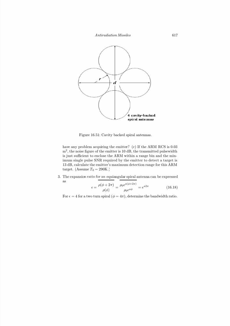
7/17/2019 1596932341 Intercept Radar.pdf
http://slidepdf.com/reader/full/1596932341-intercept-radarpdf 648/891
Antiradiation Missiles 617
Figure 16.51: Cavity backed spiral antennas.
have any problem acquiring the emitter? (c) If the ARM RCS is 0.03m2, the noise figure of the emitter is 10 dB, the transmitted pulsewidthis just sufficient to enclose the ARM within a range bin and the min-imum single pulse SNR required by the emitter to detect a target is13 dB, calculate the emitter’s maximum detection range for this ARMtarget. (Assume T
0 = 290K.)
3. The expansion ratio for an equiangular spiral antenna can be expressedas
= ρ(φ + 2π)
ρ(φ) =
ρ0ea(φ+2π)
ρ0eaφ = ea2π (16.18)
For = 4 for a two turn spiral (φ = 4π), determine the bandwidth ratio.

7/17/2019 1596932341 Intercept Radar.pdf
http://slidepdf.com/reader/full/1596932341-intercept-radarpdf 649/891

7/17/2019 1596932341 Intercept Radar.pdf
http://slidepdf.com/reader/full/1596932341-intercept-radarpdf 650/891
Chapter 17
Autonomous Classification
of LPI Radar Modulations
In this chapter, autonomous (no human operator intervention) feature extrac-tion and classification algorithms that can be used for identifying LPI radarmodulations using time-frequency (T-F) detection images are presented. Themultilayer perceptron network and the radial basis function network are pre-sented to identify the type of LPI modulation present in the interceptedsignal. These nonlinear classification networks use an input feature vector
that is generated from the T-F images (preprocessing). In the first featureextraction algorithm, the modulation energy is cropped from the T-F imageusing the marginal frequency distribution to determine the cropping region.An adaptive binarization algorithm is then used to build the feature vectorin order to preserve the high-resolution detail that emphasizes the diff erences
between modulation classes without overwhelming the classifi
cation networks.Initial classification results show that the cropping region is sensitive to high-frequency noise contained in the marginal frequency distribution. In a secondfeature extraction algorithm, lowpass filtering of the T-F image is used priorto calculation of the marginal frequency distribution. Wiener filtering of themarginal frequency distribution is also added to improve the stability of thecropping region. The use of principal components analysis to construct thefeature vector is investigated. An extended database is developed and theclassification results for simulated LPI radar modulations are shown as afunction of both SNR variations and variations in the modulation parameters(most difficult, but realistic case).
619
7/17/2019 1596932341 Intercept Radar.pdf
http://slidepdf.com/reader/full/1596932341-intercept-radarpdf 651/891
620 Detecting and Classifying LPI Radar
17.1 Classification Using Time-Frequency
Imaging
Although the automatic recognition of LPI radar modulations is a new areaof investigation, the automatic recognition of communication signal modu-lations has been of interest for many years [1—3]. In general, there are twomethods for autonomous classification of signal modulations: decision theo-retic techniques and pattern recognition techniques. In particular, researchon this topic is typically applicable to military systems. Now with the adventof software radios, research on autonomously recognizing communication sig-nal modulations has resulted in the realization of reconfigurable and adaptivewireless transceivers. The use of neural networks [4], wavelet transforms [5],higher order statistics [6], and hidden Markov models [7] have been explored.In a general sense, the autonomous recognition of communication modula-tions is an easier problem than the autonomous recognition of LPI radar
modulations due to the fact that there are only a finite number of modula-tion techniques used for communication. On the other hand, there are aninfinite number of modulation techniques that can be used for the LPI radar.In fact this is why the noncooperative intercept receiver has such a difficulttime!
Classification using T-F imaging has received considerable attention insuch diverse fields as humpback whale signal recognition [8, 9], biomedicalengineering [10, 11], underwater acoustic target detection [12], radar targetclassification [13], power grid analysis [14], and radar transmitter identifi-cation [15]. With the high degree of detail contained in the image, train-able autonomous classifiers can easily be overwhelmed by the complexity of the T-F input representation and many eff orts have been examined to re-duce this problem. Smoothing the T-F images can be used to reduce the
density of the features but will most often remove the class-distinction de-tail that the representation was intended to resolve. Quantizing the T-Frepresentation in a class- or signal-dependent manner can also preserve theneeded high-resolution detail that highlights the diff erences between classes.A vector quantization technique that is a modified version of a Kohonen’sself-organizing feature map is applied to the T-F representation in [16].
Class-dependent smoothing can also be accomplished by optimizing theT-F transformation kernel [15]. This approach eliminates the need to makea priori assumptions about the amount and type of smoothing needed andalso allows for a direct classification without the need for preprocessing toreduce the dimensionality. Optimizing the T-F kernel parameters based onthe Fisher criterion objective function is also examined in [8]. The Fishercriteria however, assume the classes have equal covariance. In [9], the T-Frepresentation is used to construct a quadratic discriminant function, whichis evaluated at specific times to form a set of statistics that are then used in a

7/17/2019 1596932341 Intercept Radar.pdf
http://slidepdf.com/reader/full/1596932341-intercept-radarpdf 652/891
Autonomous Classi fi cation of LPI Radar Modulations 621
multiple hypothesis test. The multiple hypotheses are treated simultaneouslyusing a sequentially rejective Bonferroni test to control the probability of incorrect classification.
A method based on T-F projection filtering is presented in [12]. In thisapproach the decision strategy about which target is present depends onthe comparison of a reference target and the filter output signal. In [13], areduction in the feature vector dimensionality using the geometrical momentsof the adaptive spectrogram is investigated. A principal components analysisis then used to further reduce the dimension of the feature space. This involvescalculation of the covariance matrix and its eigenvectors. The feature vectoris then formed using the eigen vectors associated to the highest eigen values,and then it is applied to a multilayer perceptron for automatic recognition.
17.2 Classification Authority and Automation
The LPI emitter has established itself as the premier tactical and strategicradar in the military spectrum. In addition to surveillance and navigation,the LPI emitter also operates in the time-critical domain for applications suchas fire control and missile guidance. In the EW battle, the noncooperativeintercept receiver is a significant element in the detection and classification of the LPI radar in a complex environment of multiple emitters and high noiseinterference. The LPI radar modulations force the intercept receiver to in-crease its processing gain by implementing T-F signal processing algorithms.With these detection techniques a human operator can examine the result-ing T-F image on a human-computer interface (HCI) and identify the type
of signal modulation present (classification) as well as quantify (or extract)the modulation parameters. The development of a corresponding jammerresponse, when required, is almost always a time critical event.
17.2.1 Human-Computer Interface Considerations
In an embedded system, cost, size, power, and complexity are limited, sothe HCI must be easy to use without sacrificing accuracy in the analysis ca-pability. Human operators are often one of the biggest sources of error inany embedded system and many operator errors are attributed to a poorlydesigned HCI [16]. Electronic intelligence (ELINT) receiver designers mustinsure that the HCI is easy and intuitive for human operators to use, but notso simple that it lulls the operator into a state of complacency and lowerstheir responsiveness to vital situations. The ELINT receiver HCI must giveappropriate feedback to the operator to allow well informed decisions to be
made based on the most up-to-date information on the electromagnetic envi-ronment. High false alarm rates will make the operator ignore a real alarmcondition. If the human operator is out of the control loop in an automated

7/17/2019 1596932341 Intercept Radar.pdf
http://slidepdf.com/reader/full/1596932341-intercept-radarpdf 653/891
622 Detecting and Classifying LPI Radar
Table 17.1: Sheridan Levels of Authority (after [18]).
Level Computer Task Human Task1 No assistance Does all2 Suggests alternatives Chooses3 Selects way to do task Schedules response4 Selects and executes Must approve5 Executes unless vetoed Has limited veto time6 Executes immediately Informed upon execution7 Executes immediately Informed if asked8 Executes immediately Ignored by computer
task, the operator will tend to adapt to the normal operation mode and not
pay close attention to the system (operator drop out). When an emergencycondition occurs, the operator’s response will be degraded and they will tendto make more mistakes. For example, the operator might unexpectedly haveto manage a proper EW response to the intercepted emitter.
17.2.2 Automation and the Human Operator
The need for human analysis of the T-F results limits these techniques toELINT receivers where the emitter information derived is not time-critical.High-level automation of the classification decision, parameter extraction andresponse management are however justified in highly time-critical situationsin which there is insufficient time for a human operator to respond and takeappropriate action [17]. This is the case for ES receivers and RWRs. Human
beings are often still needed to be the fail-safe in an otherwise automatedsystem.
The Sheridan level shown in Table 17.1 is a system of eight levels toindicate the amount of automation that is incorporated in the response, itslevel of autonomy and whether the response execution authority is assigned tothe system or to the operator [18]. The Sheridan levels or levels of authority(LoA) vary from level 1: “Computer off ers no assistance, human does all” tolevel 8: “Computer selects method, executes task and ignores human.” Inlevels 1 to 4 the operator has authority over function execution; in levels 6to 8 authority has moved to the system. In level 5 the authority is sharedbetween the system and the operator.
Figure 17.1 shows an example where the intercept receiver calculates theT-F results from an intercepted LPI signal and must then administer a jam-ming waveform response. The figure shows the EW response managementdetailing the interaction between automation, autonomy and authority for

7/17/2019 1596932341 Intercept Radar.pdf
http://slidepdf.com/reader/full/1596932341-intercept-radarpdf 654/891
Autonomous Classi fi cation of LPI Radar Modulations 623
Figure 17.1: Interaction between automation, autonomy, and authority(adapted from [17]).
the jamming waveform. Depending on the Sheridan level of the response, theT-F data is presented to the operator (arrow 1a) or used by the system part“Autonomous decision making” to decide what LPI modulation is presentand what the modulation parameters are (1b), given these T-F inputs [17].Then, the system can suggest the particular modulation type to the operator(2a), who then schedules the jamming response execution (4a) or the systemcan select and schedule an automated response (2b). Whether the executionof the scheduled jamming response must be acknowledged by the operatordepends on the LoA assigned to the response (4b). This is realized by the
“Authority filter” and the switch below the filter that determines whetherthe scheduled response is executed (3). Depending on the setting of the “Au-thority filter,” the operator does or does not receive feedback upon responseexecution (5). The interaction can be summarized as: Autonomy schedulesautomated responses, while authority allows or blocks response execution [17].
17.2.3 Autonomous Modulation Classification
Figure 17.2 shows the steps that can be used to autonomously classify theLPI radar signal modulations. The LPI radar signal is intercepted with adigital receiver that digitizes the intercepted signal. The signal is processedby both T-F and B-F detection techniques. After the T-F, B-F detectionprocessing, the resulting image planes are used by the autonomous decision
making process to identify the modulation type . The autonomous decisionmaking consists of a feature extraction algorithm that is used to derive thefeature vector from the T-F, B-F image plane. A nonlinear classification

7/17/2019 1596932341 Intercept Radar.pdf
http://slidepdf.com/reader/full/1596932341-intercept-radarpdf 655/891
624 Detecting and Classifying LPI Radar
Figure 17.2: Noncooperative intercept receiver for autonomous detection andidentification of LPI radar modulation.
network is then used to recognize the LPI signal modulation type from thefeature vector or pattern. The most important segment of this pattern recog-nition scheme is how the feature vector is formed and how it is presentedto the nonlinear classification network. Note that if a high performance re-configurable computer is used, several T-F and B-F detection/classificationalgorithms can be executed quickly and in parallel [19]. Below we first discussthe nonlinear classification networks that are used to identify the modulationtype. This includes the multilayer perceptron (MLP), and the radial basisfunction (RBF) network. Feature extraction image processing techniques arethen discussed and results are shown.
17.3 Nonlinear Classification Networks
Nonlinear classification networks use a set of processing elements (or nodes)loosely analogous to neurons in the brain (hence the name, artificial neuralnetworks). The nodes are interconnected in a network that can then identifypatterns in data as it is exposed to the data. In a sense, the network learnsfrom experience just as people do. This distinguishes neural networks fromtraditional computing programs that simply follow instructions in a fixedsequential order. The architectures are specified by: (1) the network topology,(2) the node characteristics, and (3) the training or learning rules used toconfigure the weights on each connection [20].
The classification networks can be either static or dynamic. Static net-
works are characterized by node equations that are memoryless. That is,their output is a function of only the current input and not of past or fu-ture inputs or outputs. Dynamic networks are systems with memory. The
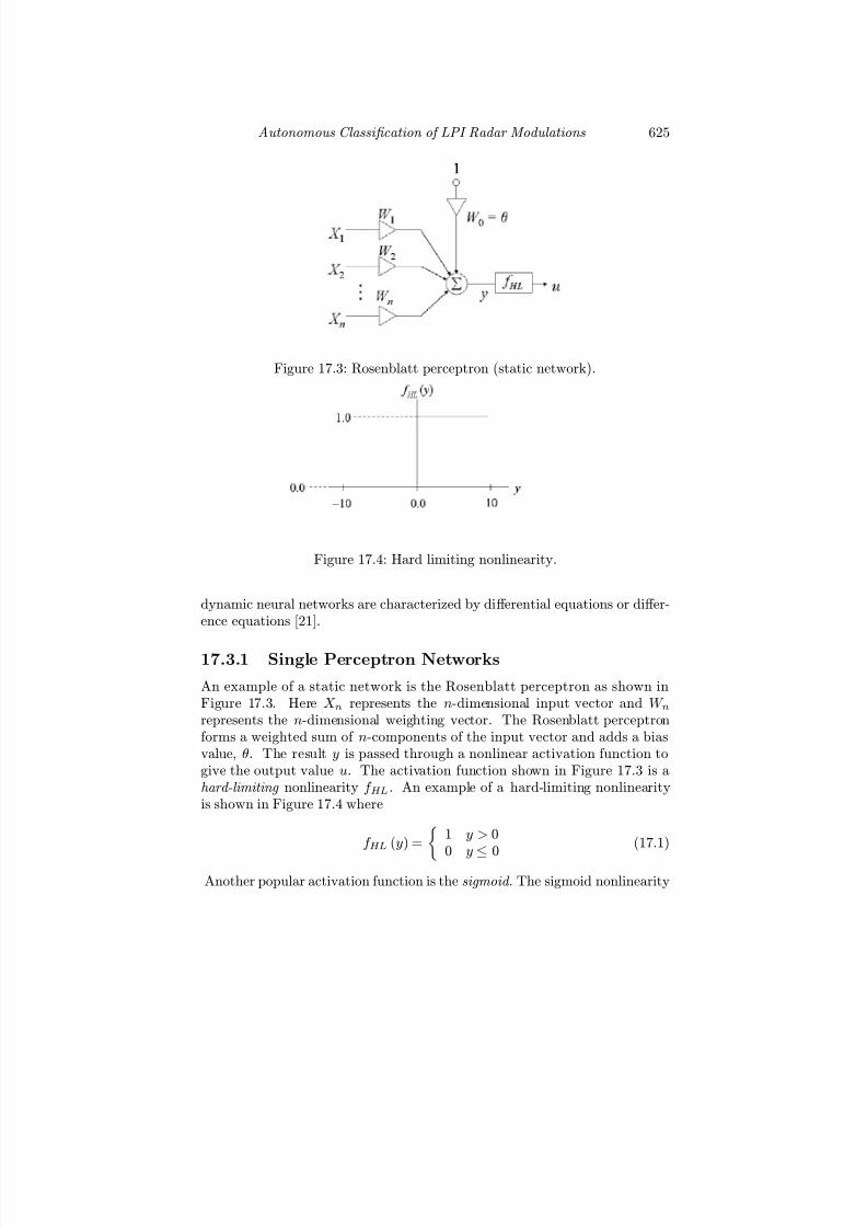
7/17/2019 1596932341 Intercept Radar.pdf
http://slidepdf.com/reader/full/1596932341-intercept-radarpdf 656/891
Autonomous Classi fi cation of LPI Radar Modulations 625
Figure 17.3: Rosenblatt perceptron (static network).
Figure 17.4: Hard limiting nonlinearity.
dynamic neural networks are characterized by diff erential equations or diff er-ence equations [21].
17.3.1 Single Perceptron Networks
An example of a static network is the Rosenblatt perceptron as shown inFigure 17.3. Here X n represents the n-dimensional input vector and W nrepresents the n-dimensional weighting vector. The Rosenblatt perceptronforms a weighted sum of n-components of the input vector and adds a biasvalue, θ. The result y is passed through a nonlinear activation function togive the output value u. The activation function shown in Figure 17.3 is ahard-limiting nonlinearity f HL . An example of a hard-limiting nonlinearityis shown in Figure 17.4 where
f HL (y) = 1 y > 00 y ≤ 0
(17.1)
Another popular activation function is the sigmoid . The sigmoid nonlinearity
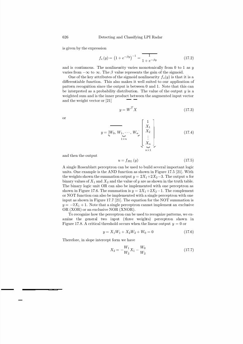
7/17/2019 1596932341 Intercept Radar.pdf
http://slidepdf.com/reader/full/1596932341-intercept-radarpdf 657/891
626 Detecting and Classifying LPI Radar
is given by the expression
f s
(y) = 1 + e−βy−1 = 1
1 + e−βy (17.2)
and is continuous. The nonlinearity varies monotonically from 0 to 1 as yvaries from −∞ to ∞. The β value represents the gain of the sigmoid.
One of the key attributes of the sigmoid nonlinearity f s(y) is that it is adiff erentiable function. This also makes it well suited to our application of pattern recognition since the output is between 0 and 1. Note that this canbe interpreted as a probability distribution. The value of the output y is aweighted sum and is the inner product between the augmented input vectorand the weight vector or [21]
y = W T
X (17.3)
or
y = [W 0, W 1, · · · , W n] 1×n
⎡⎢⎢⎢⎢⎢⎣1
X 1X 2
...X n
⎤⎥⎥⎥⎥⎥⎦ n×1
(17.4)
and then the outputu = f HL (y) (17.5)
A single Rosenblatt perceptron can be used to build several important logicunits. One example is the AND function as shown in Figure 17.5 [21]. Withthe weights shown the summation output y = 2X 1+2X 2−3. The output u for
binary values of X 1 and X 2 and the value of y are as shown in the truth table.The binary logic unit OR can also be implemented with one perceptron asshown in Figure 17.6. The summation is y = 2X 1+2X 2−1. The complementor NOT function can also be implemented with a single perceptron with oneinput as shown in Figure 17.7 [21]. The equation for the NOT summation isy = −2X 1 + 1. Note that a single perceptron cannot implement an exclusiveOR (XOR) or an exclusive NOR (XNOR).
To recognize how the perceptron can be used to recognize patterns, we ex-amine the general two input (three weights) perceptron shown inFigure 17.8. A critical threshold occurs when the linear output y = 0 or
y = X 1W 1 + X 2W 2 + W 0 = 0 (17.6)
Therefore, in slope intercept form we have
X 2 = −W 1W 2
X 1 −W 0W 2
(17.7)
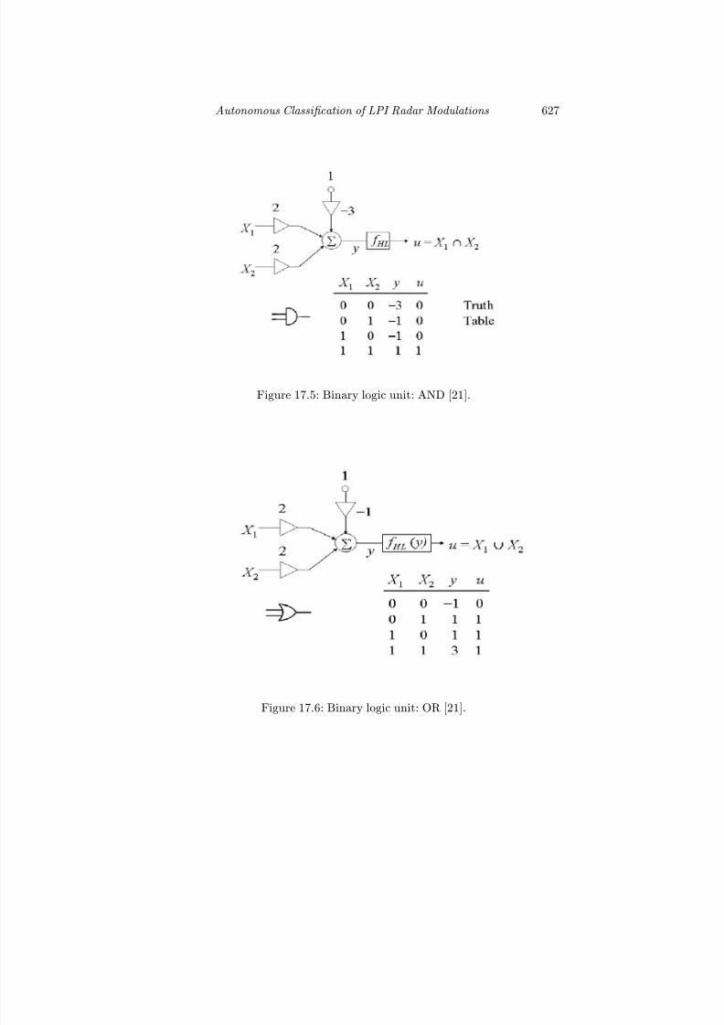
7/17/2019 1596932341 Intercept Radar.pdf
http://slidepdf.com/reader/full/1596932341-intercept-radarpdf 658/891
Autonomous Classi fi cation of LPI Radar Modulations 627
Figure 17.5: Binary logic unit: AND [21].
Figure 17.6: Binary logic unit: OR [21].
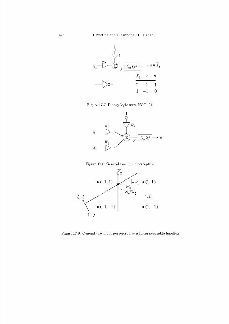
7/17/2019 1596932341 Intercept Radar.pdf
http://slidepdf.com/reader/full/1596932341-intercept-radarpdf 659/891
628 Detecting and Classifying LPI Radar
Figure 17.7: Binary logic unit: NOT [21].
Figure 17.8: General two-input perceptron.
Figure 17.9: General two-input perceptron as a linear separable function.
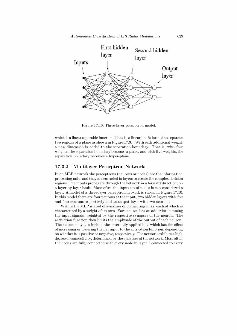
7/17/2019 1596932341 Intercept Radar.pdf
http://slidepdf.com/reader/full/1596932341-intercept-radarpdf 660/891
Autonomous Classi fi cation of LPI Radar Modulations 629
Figure 17.10: Three-layer perceptron model.
which is a linear separable function. That is, a linear line is formed to separatetwo regions of a plane as shown in Figure 17.9. With each additional weight,a new dimension is added to the separation boundary. That is, with fourweights, the separation boundary becomes a plane, and with five weights, theseparation boundary becomes a hyper-plane.
17.3.2 Multilayer Perceptron Networks
In an MLP network the perceptrons (neurons or nodes) are the informationprocessing units and they are cascaded in layers to create the complex decisionregions. The inputs propagate through the network in a forward direction, ona layer by layer basis. Most often the input set of nodes is not considered alayer. A model of a three-layer perceptron network is shown in Figure 17.10.In this model there are four neurons at the input, two hidden layers with fiveand four neurons respectively and an output layer with two neurons.
Within the MLP is a set of synapses or connecting links, each of which ischaracterized by a weight of its own. Each neuron has an adder for summingthe input signals, weighted by the respective synapses of the neuron. Theactivation function then limits the amplitude of the output of each neuron.The neuron may also include the externally applied bias which has the eff ectof increasing or lowering the net input to the activation function, depending
on whether it is positive or negative, respectively. The network exhibits a highdegree of connectivity, determined by the synapses of the network. Most oftenthe nodes are fully connected with every node in layer i connected to every
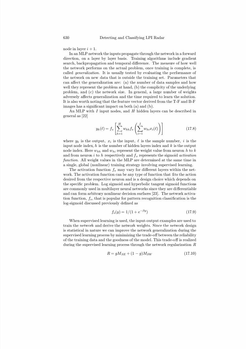
7/17/2019 1596932341 Intercept Radar.pdf
http://slidepdf.com/reader/full/1596932341-intercept-radarpdf 661/891
630 Detecting and Classifying LPI Radar
node in layer i + 1.In an MLP network the inputs propagate through the network in a forward
direction, on a layer by layer basis. Training algorithms include gradientsearch, backpropagation and temporal diff erence. The measure of how wellthe network performs on the actual problem, once training is complete, iscalled generalization . It is usually tested by evaluating the performance of the network on new data that is outside the training set. Parameters thatcan aff ect the generalization are: (a) the number of data samples and howwell they represent the problem at hand, (b) the complicity of the underlyingproblem, and (c) the network size. In general, a large number of weightsadversely aff ects generalization and the time required to learn the solution.It is also worth noting that the feature vector derived from the T-F and B-Fimages has a significant impact on both (a) and (b).
An MLP with I input nodes, and H hidden layers can be described ingeneral as [22]
yk() = f s
H h=1
wkhf s
I i=1
whixi()
(17.8)
where yk is the output, xi is the input, is the sample number, i is theinput node index, h is the number of hidden layers index and k is the outputnode index. Here wkh and whi represent the weight value from neuron h to kand from neuron i to h respectively and f s represents the sigmoid activation
function . All weight values in the MLP are determined at the same time ina single, global (nonlinear) training strategy involving supervised learning.
The activation function f s may vary for diff erent layers within the net-work. The activation function can be any type of function that fits the actiondesired from the respective neuron and is a design choice which depends on
the specific problem. Log sigmoid and hyperbolic tangent sigmoid functionsare commonly used in multilayer neural networks since they are diff erentiableand can form arbitrary nonlinear decision surfaces [23]. The network activa-tion function, f s, that is popular for pattern recognition classification is thelog-sigmoid discussed previously defined as
f s(y) = 1/(1 + e−βy) (17.9)
When supervised learning is used, the input-output examples are used totrain the network and derive the network weights. Since the network designis statistical in nature we can improve the network generalization during thesupervised learning process by minimizing the trade-off between the reliabilityof the training data and the goodness of the model. This trade-off is realized
during the supervised learning process through the network regularization R
R = gM SE + (1 − g)M SW (17.10)
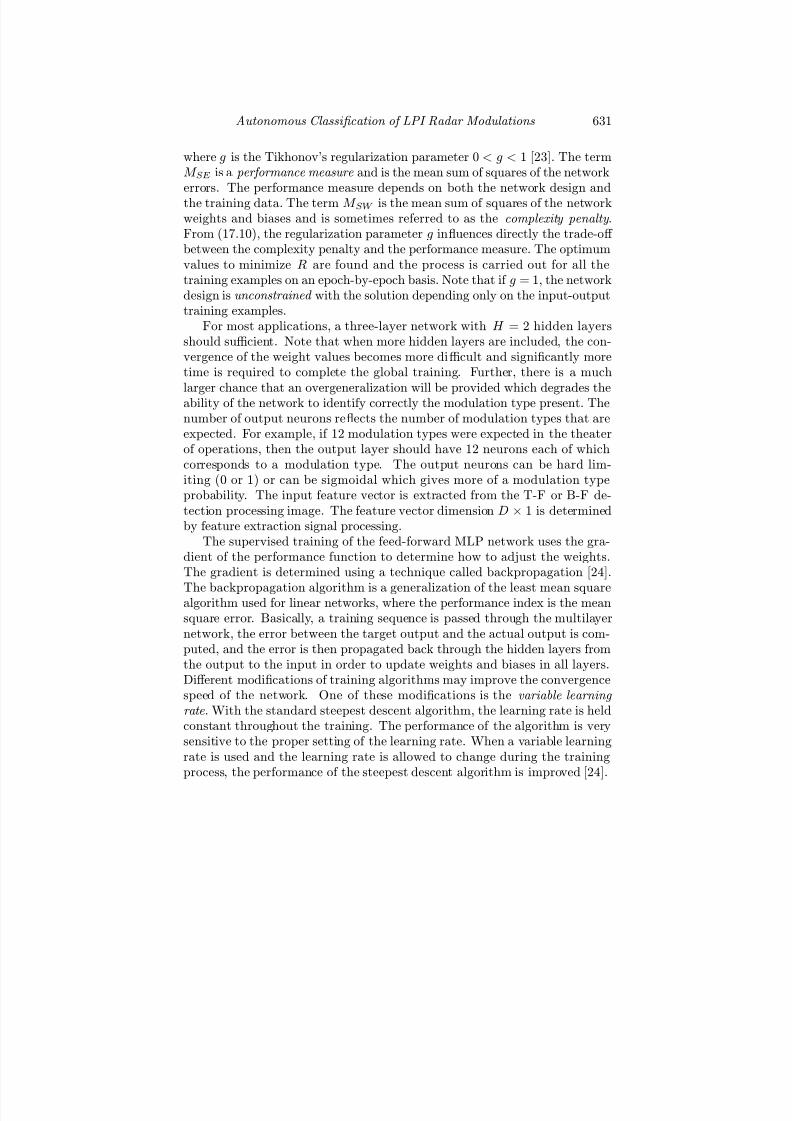
7/17/2019 1596932341 Intercept Radar.pdf
http://slidepdf.com/reader/full/1596932341-intercept-radarpdf 662/891
Autonomous Classi fi cation of LPI Radar Modulations 631
where g is the Tikhonov’s regularization parameter 0 < g < 1 [23]. The termM SE is a performance measure and is the mean sum of squares of the networkerrors. The performance measure depends on both the network design andthe training data. The term M SW is the mean sum of squares of the networkweights and biases and is sometimes referred to as the complexity penalty .From (17.10), the regularization parameter g influences directly the trade-off between the complexity penalty and the performance measure. The optimumvalues to minimize R are found and the process is carried out for all thetraining examples on an epoch-by-epoch basis. Note that if g = 1, the networkdesign is unconstrained with the solution depending only on the input-outputtraining examples.
For most applications, a three-layer network with H = 2 hidden layersshould sufficient. Note that when more hidden layers are included, the con-vergence of the weight values becomes more difficult and significantly moretime is required to complete the global training. Further, there is a much
larger chance that an overgeneralization will be provided which degrades theability of the network to identify correctly the modulation type present. Thenumber of output neurons reflects the number of modulation types that areexpected. For example, if 12 modulation types were expected in the theaterof operations, then the output layer should have 12 neurons each of whichcorresponds to a modulation type. The output neurons can be hard lim-iting (0 or 1) or can be sigmoidal which gives more of a modulation typeprobability. The input feature vector is extracted from the T-F or B-F de-tection processing image. The feature vector dimension D × 1 is determinedby feature extraction signal processing.
The supervised training of the feed-forward MLP network uses the gra-dient of the performance function to determine how to adjust the weights.The gradient is determined using a technique called backpropagation [24].
The backpropagation algorithm is a generalization of the least mean squarealgorithm used for linear networks, where the performance index is the meansquare error. Basically, a training sequence is passed through the multilayernetwork, the error between the target output and the actual output is com-puted, and the error is then propagated back through the hidden layers fromthe output to the input in order to update weights and biases in all layers.Diff erent modifications of training algorithms may improve the convergencespeed of the network. One of these modifications is the variable learning
rate . With the standard steepest descent algorithm, the learning rate is heldconstant throughout the training. The performance of the algorithm is verysensitive to the proper setting of the learning rate. When a variable learningrate is used and the learning rate is allowed to change during the trainingprocess, the performance of the steepest descent algorithm is improved [24].
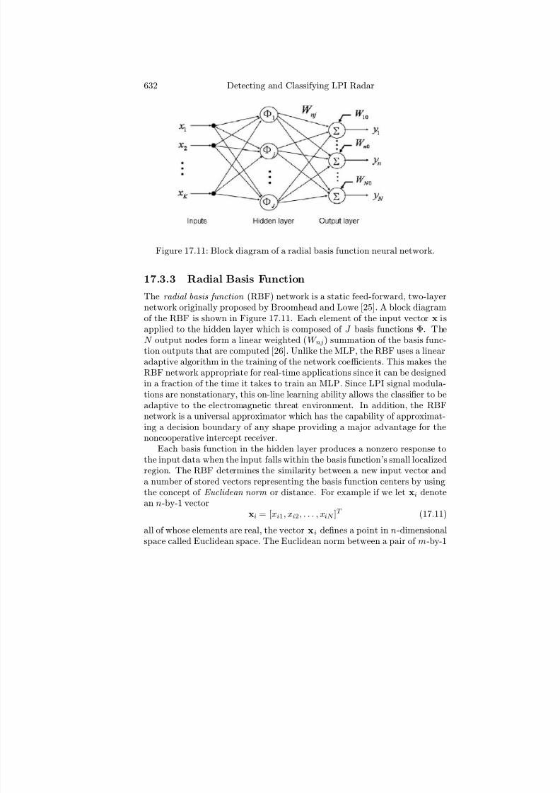
7/17/2019 1596932341 Intercept Radar.pdf
http://slidepdf.com/reader/full/1596932341-intercept-radarpdf 663/891
632 Detecting and Classifying LPI Radar
Figure 17.11: Block diagram of a radial basis function neural network.
17.3.3 Radial Basis Function
The radial basis function (RBF) network is a static feed-forward, two-layernetwork originally proposed by Broomhead and Lowe [25]. A block diagramof the RBF is shown in Figure 17.11. Each element of the input vector x isapplied to the hidden layer which is composed of J basis functions Φ. TheN output nodes form a linear weighted (W nj) summation of the basis func-tion outputs that are computed [26]. Unlike the MLP, the RBF uses a linearadaptive algorithm in the training of the network coefficients. This makes theRBF network appropriate for real-time applications since it can be designedin a fraction of the time it takes to train an MLP. Since LPI signal modula-tions are nonstationary, this on-line learning ability allows the classifier to beadaptive to the electromagnetic threat environment. In addition, the RBF
network is a universal approximator which has the capability of approximat-ing a decision boundary of any shape providing a major advantage for thenoncooperative intercept receiver.
Each basis function in the hidden layer produces a nonzero response tothe input data when the input falls within the basis function’s small localizedregion. The RBF determines the similarity between a new input vector anda number of stored vectors representing the basis function centers by usingthe concept of Euclidean norm or distance. For example if we let xi denotean n-by-1 vector
xi = [xi1, xi2, . . . , xiN ]T (17.11)
all of whose elements are real, the vector xi defines a point in n-dimensionalspace called Euclidean space. The Euclidean norm between a pair of m-by-1

7/17/2019 1596932341 Intercept Radar.pdf
http://slidepdf.com/reader/full/1596932341-intercept-radarpdf 664/891
Autonomous Classi fi cation of LPI Radar Modulations 633
vectors xi and xj is defined as
||xi − xj || = nk=1
(xik − xjk)21/2
(17.12)
where xik and xjk are the kth elements of the input vectors xi and xj respec-tively [23]. Correspondingly, the similarity between the inputs represented byxik and xjk is defined as the reciprocal of the Euclidean distance ||xi − xj ||.
The output of the RBF can be expressed as
y pn = W n0 +J j=1
W njΦ(||x p − cj ||) (17.13)
where y pn is the output of the nth modulation node in response to the pthinput pattern, Φ(||x p − cn||) is the output of the hidden node n in responseto the pth input vector x p and the vectors cn, n = 1, . . . , N are referred to asthe centers of the radially symmetric basis functions Φ. The weighting matrixW nj represents the synaptic weights from the j th radial basis function to thenth modulation output node and W n0 is the bias or threshold assigned to thenth modulation output node.
One symmetrical choice for the radial basis function Φ is the Gaussianfunction
Φ(||x p − cn||) = exp
⎧⎨⎩−
J j=1
(xj − cnj)2
2σ2nj
⎫⎬⎭ (17.14)
where σnj are the elements of a covariance matrix (or spread), which is takenhere to be diagonal.
The set of hidden units consist of a set of functions which constitute an
arbitrary basis for the feature vector patterns to be classified when expandedinto hidden unit space. These are referred to as radial basis functions. Theexpansion of input vectors into a hidden unit space of relatively high dimen-sion (many radial basis functions) will result in a greater likelihood of theclassification problem becoming linearly separable. One approach for an ef-ficient RBF network design is by iteratively creating the RBF one neuronat a time. Neurons are added to the network until either the sum-squarederror falls beneath an error goal or a maximum number of neurons has beenreached [23]. The two parameters used to optimize the RBF to obtain a bet-ter probability of correct classification are the goal and spread σ . The spreadconstant should be larger than the distance between adjacent input vectors,so as to get a good generalization, but smaller than the distance across thewhole input space. The training is accomplished in two stages. The basis
functions are determined by unsupervised techniques using the input datawhile the second layer weights are found by a fast linear supervised method.Hence the training is fast and efficient.

7/17/2019 1596932341 Intercept Radar.pdf
http://slidepdf.com/reader/full/1596932341-intercept-radarpdf 665/891
634 Detecting and Classifying LPI Radar
17.4 Feature Extraction Signal Processing
In Figure 17.2, the LPI signal is detected with three T-F signal processing
methods. Each T-F image contains features that identify the modulation type(and its parameters). Methods to autonomously extract these features fromthe T-F distribution have recently received much attention (see for example[27, 28]). Two efficient feature extraction methods that build a feature vector
from a T-F image are described below.
17.4.1 Marginal Frequency Adaptive Binarization
An autonomous (no human operator intervention) T-F feature extractionimage processing approach that can be used for classification of LPI radarmodulations is examined. The feature extraction image processing uses themarginal frequency distribution, or instantaneous energy [29], derived fromthe T-F representation in order to isolate the location of the modulation au-tonomously. In order to isolate the modulation, a histogram of the normalizedmarginal frequency distribution is first computed to choose a threshold forcomparison against the mean energy value calculated from the convolutionof the normalized marginal frequency distribution with an averaging kernel(sliding window) of length n. This convolution gives the start and stop fre-quency of the modulation energy. With the location of the modulation energyknown it is possible to crop the energy from within the T-F image and com-pute a feature vector for input into the classification network. In order topreserve the high-resolution detail that emphasizes the diff erences betweenmodulation classes without overwhelming the classifier, an adaptive binariza-tion algorithm is used to generate a vector of 1’s and 0’s that represent themodulation [30].
A block diagram of the autonomous feature extraction image processingtechnique is shown in Figure 17.12. This technique uses the T-F marginalfrequency distribution and an adaptive binarization algorithm to form thefeature vector. The Choi-Williams detection of a T1(2) signal modulation isused to demonstrate the marginal frequency adaptive binarization (MFAB)feature extraction algorithm.
Deleting No-Signal Region
One of the characteristics that may be present in the T-F image is whenthe signal does not extend for the entire distribution. The T-F image willthen show the presence of a black column starting where the signal ends andcovering all frequencies. Since this no-signal region within the T-F image doesnot contain useful information for classification, this region must be removed(see the detect & delete no-signal region block in Figure 17.12). Figure 17.13

7/17/2019 1596932341 Intercept Radar.pdf
http://slidepdf.com/reader/full/1596932341-intercept-radarpdf 666/891
Autonomous Classi fi cation of LPI Radar Modulations 635
Figure 17.12: Autonomous feature extraction using the marginal frequencyadaptive binarization (MFAB) algorithm [30].
shows the no-signal region within a Choi-Williams distribution for a T1(2)modulation. Also shown is the image with the no-signal region removed.
Marginal Frequency Distribution to Determine Cropping
The marginal frequency distribution off ers a way to examine a T-F image inintercept situations where there is a low SNR [30]. The marginal frequencydistribution gives the instantaneous energy of the signal as a function of frequency. The marginal frequency distribution is generated by
CWDx(ω) = CWDx(,ω) (17.15)
or summing the time values for each frequency in the T-F image and then stor-ing the sums in an array. Each marginal frequency distribution is a uniquerepresentation of the T-F image it was generated from. The marginal fre-quency distribution is normalized by dividing the sums by the largest sumin the array. The normalized marginal frequency distribution of the T1(2)modulation is shown in Figure 17.14.
The normalized distribution is used to extract a threshold that is usedlater to isolate and crop the modulation energy within the T-F image. Thethreshold is determined by generating a histogram of 100 bins of the nor-malized marginal frequency distribution and then taking the value from thehistogram bin which generates the best probability of correct classi fi cation
(Pcc) results. An example of the T1(2) histogram is shown in Figure 17.15.Once the threshold is determined (n = 9) the convolution of the aver-
aging kernel with the normalized marginal frequency distribution is used to

7/17/2019 1596932341 Intercept Radar.pdf
http://slidepdf.com/reader/full/1596932341-intercept-radarpdf 667/891
636 Detecting and Classifying LPI Radar
Figure 17.13: Choi-Williams T-F image for the T1(2) modulation showing(a) presence of the no-signal region and (b) no-signal region removed.
Figure 17.14: Normalized marginal frequency distribution of the T1(2) mod-
ulation shown in Figure 17.13.

7/17/2019 1596932341 Intercept Radar.pdf
http://slidepdf.com/reader/full/1596932341-intercept-radarpdf 668/891
Autonomous Classi fi cation of LPI Radar Modulations 637
Figure 17.15: Histogram of the normalized marginal frequency distributionfor T1(2) modulation used to determine threshold autonomously.
determine the start and stop cropping locations of the modulation energy.The convolution operation calculates the mean of the corresponding cells inthe normalized distribution and compares it to the threshold identified fromthe histogram. If the average of the convolution is greater than the thresholdthe start of the modulation energy is found. To find the stop location thesame convolution algorithm is used but the kernel is initialized at the endof the normalized distribution. With the location of the modulation energy
known it can be cropped from the original image as shown in Figure 17.16.
Adaptive Binarization
An adaptive binarization algorithm is used to generate a binary image that isthen resized to form a feature (column) vector containing ones and zeros. Ablock diagram of the adaptive binarization process is shown in Figure 17.17[30]. The intensity image |I (t,ω)| is normalized I (t,ω) with respect to thelargest value in the image, where the pixel values 0 ≤ I (t,ω) ≤ 1.
A histogram of the intensity level content, h(n), is then generated usingN = 50 bins. The cumulative distribution function is computed using thishistogram as
cdf (n) = ni=1 h(i)N n=1 h(n) (17.16)
A cdf threshold, C , is chosen and the intensity bin n where cdf (n) ≥ C is
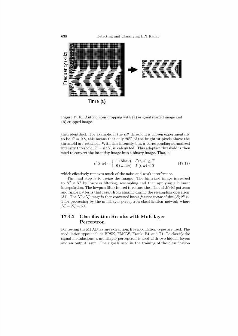
7/17/2019 1596932341 Intercept Radar.pdf
http://slidepdf.com/reader/full/1596932341-intercept-radarpdf 669/891
638 Detecting and Classifying LPI Radar
Figure 17.16: Autonomous cropping with (a) original resized image and(b) cropped image.
then identified. For example, if the cdf threshold is chosen experimentallyto be C = 0.8, this means that only 20% of the brightest pixels above thethreshold are retained. With this intensity bin, a corresponding normalizedintensity threshold, T = n/N , is calculated. This adaptive threshold is thenused to convert the intensity image into a binary image. That is,
I (t,ω) =
1 (black) I (t,ω) ≥ T 0 (white) I (t,ω) < T
(17.17)
which eff ectively removes much of the noise and weak interference.The final step is to resize the image. The binarized image is resized
to N r × N c by lowpass filtering, resampling and then applying a bilinearinterpolation. The lowpass filter is used to reduce the eff ect of Moire patternsand ripple patterns that result from aliasing during the resampling operation[31]. The N r×N c image is then converted into a feature vector of size (N rN c)×1 for processing by the multilayer perceptron classification network whereN r = N c = 50.
17.4.2 Classification Results with Multilayer
Perceptron
For testing the MFAB feature extraction, five modulation types are used. The
modulation types include BPSK, FMCW, Frank, P4, and T1. To classify thesignal modulations, a multilayer perceptron is used with two hidden layersand an output layer. The signals used in the training of the classification
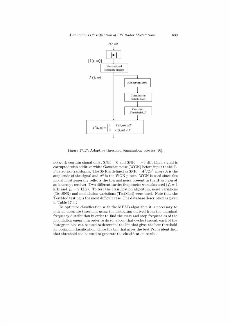
7/17/2019 1596932341 Intercept Radar.pdf
http://slidepdf.com/reader/full/1596932341-intercept-radarpdf 670/891
Autonomous Classi fi cation of LPI Radar Modulations 639
Figure 17.17: Adaptive threshold binarization process [30].
network contain signal only, SNR = 0 and SNR = −3 dB. Each signal iscorrupted with additive white Gaussian noise (WGN) before input to the T-
F detection transforms. The SNR is defined as SNR = A2/2σ2 where A is theamplitude of the signal and σ2 is the WGN power. WGN is used since thismodel most generally reflects the thermal noise present in the IF section of an intercept receiver. Two diff erent carrier frequencies were also used (f c = 1kHz and f c = 2 kHz). To test the classification algorithm, noise variations(TestSNR) and modulation variations (TestMod) were used. Note that theTestMod testing is the most difficult case. The database description is givenin Table 17.4.2.
To optimize classification with the MFAB algorithm it is necessary topick an accurate threshold using the histogram derived from the marginalfrequency distribution in order to find the start and stop frequencies of themodulation energy. In order to do so, a loop that cycles through each of thehistogram bins can be used to determine the bin that gives the best thresholdfor optimum classification. Once the bin that gives the best Pcc is identified,that threshold can be used to generate the classification results.
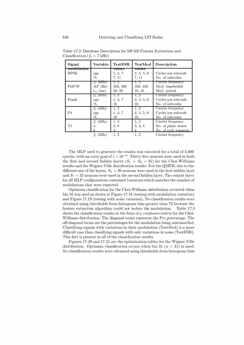
7/17/2019 1596932341 Intercept Radar.pdf
http://slidepdf.com/reader/full/1596932341-intercept-radarpdf 671/891
640 Detecting and Classifying LPI Radar
Table 17.2: Database Description for MFAB Feature Extraction andClassification (f s = 7 kHz)
Signal Variable TestSNR TestMod Descriptionmodulation values valuesBPSK cpp 1, 4, 7 2, 3, 5, 6 Cycles p er sub code
N c 7, 11 7, 11 No. of subcodesf c (kHz) 1, 2 1, 2 Carrier frequency
FMCW ∆F (Hz) 250, 500 350, 450 Mo d. bandwidthtm (ms) 20, 50 35, 45 Mod. periodf c (kHz) 1, 2 1, 2 Carrier frequency
Frank cpp 1, 4, 7 2, 3, 5, 6 Cycles p er sub codeN c 16 16 No. of subcodesf c (kHz) 1, 2 1, 2 Carrier frequency
P4 cpp 1, 4, 7 2, 3, 5, 6 Cycles p er sub codeN c 16 16 No. of subcodes
f c (kHz) 1, 2 1, 2 Carrier frequencyT1 n 2, 6 3, 4, 5 No. of phase states
k 4 4 No. of code segmentsf c (kHz) 1, 2 1, 2 Carrier frequency
The MLP used to generate the results was executed for a total of 5,000epochs, with an error goal of 1 × 10⁻⁶. Thirty-five neurons were used in boththe first and second hidden layers (S 1 = S 2 = 35) for the Choi-Williamsresults and the Wigner-Ville distribution results. For the QMFB, due to thediff erent size of the layers, S 1 = 20 neurons were used in the first hidden layerand S 2 = 35 neurons were used in the second hidden layer. The output layer
for all MLP confi
gurations contained 5 neurons which matches the number of modulations that were expected.Optimum classification for the Choi-Williams distribution occurred when
bin 16 was used as shown in Figure 17.18 (testing with modulation variation)and Figure 17.19 (testing with noise variation). No classification results wereobtained using thresholds from histogram bins greater than 72 because thefeature extraction algorithm could not isolate the modulation. Table 17.3shows the classification results in the form of a confusion matrix for the Choi-Williams distribution. The diagonal terms represent the Pcc percentage. Theoff -diagonal terms are the percentages for the modulation being misclassified.Classifying signals with variations in their modulation (TestMod) is a moredifficult case than classifying signals with only variations in noise (TestSNR).This fact is present in all of the classification results.
Figures 17.20 and 17.21 are the optimization tables for the Wigner-Villedistribution. Optimum classification occurs when bin 31 (n = 31) is used.No classification results were obtained using thresholds from histogram bins

7/17/2019 1596932341 Intercept Radar.pdf
http://slidepdf.com/reader/full/1596932341-intercept-radarpdf 672/891
Autonomous Classi fi cation of LPI Radar Modulations 641
Figure 17.18: Choi-Williams: MLP optimization (TestMod).
Figure 17.19: Choi-Williams: MLP optimization (TestSNR).

7/17/2019 1596932341 Intercept Radar.pdf
http://slidepdf.com/reader/full/1596932341-intercept-radarpdf 673/891
642 Detecting and Classifying LPI Radar
Table 17.3: Choi-Williams MLP Classification Confusion Matrix (n = 16)
TestMod BPSK FMCW Frank P4 T1BPSK 0.93 0.0 0.08 0.35 0.08
FMCW 0.00 1.0 0.01 0.00 0.00Frank 0.01 0.0 0.53 0 .05 0.07
P4 0.05 0.0 0.35 0.60 0.02T1 0.01 0.0 0.04 0.00 0.83
TestSNR BPSK FMCW Frank P4 T1BPSK 0.96 0.00 0.22 0.11 0.12
FMCW 0.00 1.0 0.00 0.00 0.00
Frank 0.01 0.0 0.74 0 .02 0.03
P4 0.03 0.0 0.01 0.85 0.05T1 0.00 0.0 0.03 0.01 0.81
greater than 66 because the feature extraction algorithm could not isolate themodulation. Table 17.4 shows the classification results for the Wigner-Villedistribution when bin 31 is used.
Figures 17.22 and 17.23 are the optimization tables for the QMFB detec-tion technique. Optimum classification occurs when bin 9 (n = 9) is used.No classification results were obtained using thresholds from histogram binsgreater than 18 because the feature extraction algorithm could not isolatethe modulation. Table 17.5 shows the classification results for the QMFBdistribution when bin 9 is used.
17.4.3 Classification Results with Radial Basis
Function Network
To produce optimum results with the RBF it is necessary to pick an ac-curate threshold using the histogram derived from the marginal frequencydistribution in order to accurately find the start and stop frequencies of themodulation energy similar to what was done for the MLP. The optimum clas-sification occurs when bin 16 (n = 16) is used. Table 17.6 shows the classifica-tion using the RBF and the Choi-Williams for n = 16. For the Wigner-Villedistribution, the optimum classification occurs when bin 58 (n = 58) is used.Table 17.7 shows the classification using the RBF and the Wigner-Ville distri-bution for n = 16. For the quadrature mirror filtering, the optimum classifica-tion occurs when bin 14 (n = 14) is used. Table 17.8 shows the classificationusing the RBF and the Wigner-Ville distribution for n = 16.

7/17/2019 1596932341 Intercept Radar.pdf
http://slidepdf.com/reader/full/1596932341-intercept-radarpdf 674/891
Autonomous Classi fi cation of LPI Radar Modulations 643
Figure 17.20: Wigner-Ville distribution: MLP optimization (TestMod).
Figure 17.21: Wigner-Ville distribution: MLP optimization (TestSNR).

7/17/2019 1596932341 Intercept Radar.pdf
http://slidepdf.com/reader/full/1596932341-intercept-radarpdf 675/891
644 Detecting and Classifying LPI Radar
Table 17.4: Wigner-Ville MLP Classification Confusion Matrix (n = 31)
TestMod BPSK FMCW Frank P4 T1
BPSK 0.96 0.0 0.08 0.12 0.20
FMCW 0.00 1.0 0.00 0.00 0.00Frank 0.02 0.0 0.58 0 .22 0.27
P4 0.02 0.0 0.33 0.65 0.04
T1 0.01 0.0 0.00 0.01 0.49
TestSNR BPSK FMCW Frank P4 T1
BPSK 0.95 0.00 0.19 0.06 0.10
FMCW 0.00 1.0 0.00 0.00 0.01Frank 0.02 0.0 0.76 0 .01 0.02
P4 0.01 0.0 0.03 0.91 0.01
T1 0.02 0.0 0.03 0.02 0.86
Figure 17.22: Quadrature mirror filtering: MLP optimization (TestMod).

7/17/2019 1596932341 Intercept Radar.pdf
http://slidepdf.com/reader/full/1596932341-intercept-radarpdf 676/891
Autonomous Classi fi cation of LPI Radar Modulations 645
Figure 17.23: Quadrature mirror filtering: MLP optimization (TestSNR).
Table 17.5: Quadrature Mirror Filtering MLP Classification ConfusionMatrix (n = 9)
TestMod BPSK FMCW Frank P4 T1
BPSK 0.82 0.40 0.48 0.35 0.23
FMCW 0.14 0.48 0.21 0.21 0.00Frank 0.01 0.01 0.13 0 .14 0.05
P4 0.03 0.11 0.18 0.30 0.02
T1 0.00 0.0 0.01 0.00 0.70
TestSNR BPSK FMCW Frank P4 T1
BPSK 0.95 0.03 0.08 0.11 0.09
FMCW 0.01 0.94 0.03 0.01 0.01Frank 0.02 0.02 0.81 0 .01 0.03
P4 0.02 0.02 0.03 0.86 0.04
T1 0.00 0.00 0.05 0.01 0.85

7/17/2019 1596932341 Intercept Radar.pdf
http://slidepdf.com/reader/full/1596932341-intercept-radarpdf 677/891
646 Detecting and Classifying LPI Radar
Table 17.6: Choi-Williams RBF Classification Confusion Matrix (n = 16)
TestMod BPSK FMCW Frank P4 T1
BPSK 1.00 0.00 0.0 0.00 0.17
FMCW 0.00 1.00 0.00 0.00 0.00Frank 0.00 0.00 0.50 0 .14 0.05
P4 0.00 0.00 0.38 0.88 0.00
PT1 0.00 0.00 0.13 0.03 0.83
TestSNR BPSK FMCW Frank P4 T1
BPSK 0.95 0.00 0.07 0.07 0.00
FMCW 0.00 1.00 0.00 0.00 0.00Frank 0.00 0.00 0.87 0 .00 0.00
P4 0.02 0.00 0.03 0.90 0.10PT1 0.03 0.00 0.03 0.03 0.90
Table 17.7: Wigner-Ville Distribution RBF Classification Confusion Matrix(n = 58)
TestMod BPSK FMCW Frank P4 T1BPSK 0.75 0.00 0.00 0.00 0.00
FMCW 0.00 1.00 0.13 0.00 0.00Frank 0.00 0.00 0.50 0 .38 0.00
P4 0.00 0.00 0.25 0.50 0.00
T1 0.25 0.00 0.13 0.13 1.00
TestSNR BPSK FMCW Frank P4 T1
BPSK 0.83 0.00 0.07 0.03 0.00
FMCW 0.03 1.00 0.00 0.00 0.00Frank 0.00 0.00 0.70 0 .10 0.05
P4 0.02 0.00 0.07 0.83 0.10
T1 0.13 0.00 0.17 0.03 0.95

7/17/2019 1596932341 Intercept Radar.pdf
http://slidepdf.com/reader/full/1596932341-intercept-radarpdf 678/891
Autonomous Classi fi cation of LPI Radar Modulations 647
Table 17.8: Wigner-Ville Distribution RBF Classification Confusion Matrix(n = 58)
TestMod BPSK FMCW Frank P4 T1
BPSK 0.81 0.25 0.75 0.63 0.67FMCW 0.19 0.50 0.13 0.25 0.00
Frank 0.00 0.00 0.13 0 .00 0.00P4 0.00 0.25 0.00 0.13 0.00
T1 0.00 0.00 0.00 0.00 0.80
TestSNR BPSK FMCW Frank P4 T1
BPSK 0.97 0.00 0.10 0.10 0.20
FMCW 0.03 1.00 0.17 0.07 0.00
Frank 0.00 0.00 0.73 0 .00 0.00P4 0.02 0.00 0.00 0.83 0.00
T1 0.00 0.00 0.00 0.00 0.80
17.4.4 Discussion of Classification Results
The marginal frequency adaptive binarization (MFAB) algorithm was able tobe applied to a complex database of LPI signals that closely resembles thetypes of signals that are found operationally. The ADC sampling frequency(f s = 7, 000 Hz) and LPI signal frequencies and bandwidths are considerablylower than those within the actual intercept receiver hardware due to compu-tational considerations. The classification results however, are representativeof the type of results that would be obtained using actual LPI emitters andintercept receiver hardware. The success of the MFAB feature extraction al-gorithm is due in part to the user’s ability to choose the cropping threshold
from an optimization analysis. Choosing the optimum threshold ensures thatthe algorithm is able to isolate the modulation energy and produce the bestpossible results for the signal types that are expected.
The best classification results were produced with the Choi-Williams dis-tribution. It might be suggested that the success of using the Choi-Williamsdistribution is attributed to its lack of cross terms (compared to the Wigner-Ville distribution), which can confuse the classification network. That is, thelarge cross-terms are not conducive to producing unique T-F features thatcan help the classifier distinguish the diff erent signal modulations from oneanother.
The MLP consistently produced better results than the RBF. The MLPwas successful because it had more variables that could be configured to pro-duce optimum results. The only variable in the RBF that could be changedwas the spread. While the results from the RBF were not as good as thoseseen coming from the MLP the RBF does have an advantage in terms of its

7/17/2019 1596932341 Intercept Radar.pdf
http://slidepdf.com/reader/full/1596932341-intercept-radarpdf 679/891
648 Detecting and Classifying LPI Radar
application to an operational environment. Its training phase is fast and effi-cient. Because it trains faster than the MLP, in an operational environmenta user would not have to wait long before receiving classification results foran LPI signal. This feature of the RBF is important and should be investi-gated in an attempt to improve the RBF’s results so that it can be appliedoperationally. In the next section, several signal processing changes are madein order to improve the classification results.
17.5 Modified Feature Extraction Signal
Processing
Calculation of the cropping region using the marginal frequency distributionallows the low frequency LPI modulation to be retained and the remainingT-F regions to be discarded. It is important that the size of the cropping
region be adaptive and only contain the modulation energy so that the de-rived feature vector is consistently correlated with the modulation type. Inthe cropping technique described above, the presence of high frequency noisewithin the T-F image however, can vary the size of the cropping window.To minimize this eff ect, the use of a lowpass filter prior to the calculation of the marginal frequency distribution is investigated to help achieve the mostconsistent cropping of the modulation energy. To make the threshold calcu-lation more robust, the marginal frequency distribution is smoothed using aWiener filter before normalization. The Wiener filter takes the form of a linearadaptive filter which adjusts its free parameters in response to the statisticalvariations in the marginal frequency distribution. Also as an alternative todirectly using the feature vector as input to the classifier, this section alsoexamines the use of principal components analysis (PCA) in order to develop
a lower dimensional feature vector for use by the classifier. A block diagramof the modified autonomous T-F cropping and feature extraction algorithmis shown in Figure 17.24 [32].
17.5.1 Lowpass Filtering for Cropping Consistency
The detect and delete no-signal region is followed by a low pass filter (LPF)applied to the T-F image. This insures that the low frequency LPI modulationenergy is preserved and the high frequency noise is removed. The filteringcan easily be performed in the frequency domain. Frequency domain filteringusing the 2-D Fourier transform is fast and efficient. Let f (k1, k2) for k1 =0, 1, 2, . . . , M − 1 and k2 = 0, 1, 2, . . . , N − 1 denote the M × N T-F image.The 2-D discrete Fourier transform (DFT) of f denoted by F (u, v) is [33]
F (u, v) =M −1k1=0
N −1k2=0
f (k1, k2)e−j2π(uk1/M +vk2/N ) (17.18)

7/17/2019 1596932341 Intercept Radar.pdf
http://slidepdf.com/reader/full/1596932341-intercept-radarpdf 680/891
Autonomous Classi fi cation of LPI Radar Modulations 649
Figure 17.24: Modified T-F autonomous cropping and feature extractionalgorithm.
for u = 0, 1, 2, . . . , M − 1 and v = 0, 1, 2, . . . , N − 1. The M × N rectangu-lar region F (u, v), defined by u and v, is often referred to as the frequencyrectangle and is the same size as the input image. Note that the frequencyrectangle can also be defined by digital frequencies as shown in Figure 17.25where ω1 = 2πu/M and ω2 = 2πv/N .
Given F (u, v), f (k1, k2) can be obtained by means of the inverse DFT.
Both DFT and inverse DFT are obtained in practice using a fast 2-D Fouriertransform (FFT) algorithm [33]. The convolution theorem, which is the foun-dation for linear filtering in both spatial and frequency domains, can be writ-ten as follows
f (k1, k2) ∗ h(k1, k2) ⇔ H (u, v)F (u, v) (17.19)
and conversely,
f (k1, k2)h(k1, k2) ⇔ H (u, v) ∗ F (u, v) (17.20)
Filtering in the spatial domain consists of convolving an image f (k1, k2) witha filter mask, h(k1, k2). According to the convolution theorem, the sameresult can be obtained in the frequency domain by multiplying F (u, v) byH (u, v), which is referred to as the filter transfer function. A block diagram
of the frequency domain filtering process is shown in Figure 17.26.The filter transfer function H (u, v) can be obtained in three steps. First,
the desired frequency response (ideal lowpass filter) H d(u, v) is created as a
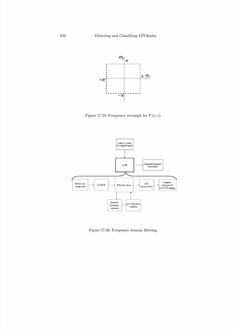
7/17/2019 1596932341 Intercept Radar.pdf
http://slidepdf.com/reader/full/1596932341-intercept-radarpdf 681/891
650 Detecting and Classifying LPI Radar
Figure 17.25: Frequency rectangle for F (u, v).
Figure 17.26: Frequency domain fi
ltering.

7/17/2019 1596932341 Intercept Radar.pdf
http://slidepdf.com/reader/full/1596932341-intercept-radarpdf 682/891
Autonomous Classi fi cation of LPI Radar Modulations 651
matrix. An ideal lowpass filter has the transfer function [33]
H d(u, v) = 1 if D(u, v) ≤ D0
0 if D(u, v) ≥ D0 (17.21)
where D0 (cutoff parameter) is a specified nonnegative number and D(u, v)is the distance from point (u, v) to the center of the filter. D0 can also bedefined as the normalized value of digital frequencies ω1,ω2 by π. Second,a two-dimensional Gaussian window is created with a standard deviationσ = N × D0/8 where N is the number of columns in the image. The standarddeviation of the window is related to D0, and the structure becomes adaptiveto the changes in the desired frequency responses. For the detection of LPIemitter modulations, both the frequency response matrix and the Gaussianwindow have dimensions of M × N which is equal to the image dimensionf (k1, k2) and the 2-D FFT output dimension F (u, v). The last step is tomultiply H d(u, v) by the Gaussian window.
The transfer function of the Gaussian lowpass filter obtained by this mul-tiplication process is then given by [34]
H (u, v) = eD2(u,v)/2σ2 (17.22)
These steps are illustrated in Figure 17.27. Figure 17.27(a) shows the desiredfrequency response with D0 = 0.3 (where |D0| ∈ [0, 1]) or ω1 = ω2 = 0.3π,Figure 17.27(b) shows the Gaussian window with σ = N × D0/8 = 33.825.The dimension of both the frequency response matrix and Gaussian window isM = 1,024, N = 902. Figure 17.27(c) shows the resultant Gaussian lowpassfilter and Figure 17.27(d) shows the Gaussian lowpass filter as an image.Several values of ω1,ω2 can be tested during the simulation process to findan optimum value for each distribution. For each trial the digital cutoff
frequencies should be set to ω1 = ω2. After obtaining the lowpass filter,the frequency domain filtering can be implemented by multiplying F (u, v) byH (u, v). This operation is followed by shifting the frequency components backand taking the inverse FFT of the filtered image. The last step is obtainingthe real part of the inverse FFT.
17.5.2 Calculating the Marginal Frequency Distribution
After the LPF is used to eliminate the high frequency noise, the marginalfrequency distribution of the T-F image is calculated. The marginal frequencydistribution gives the instantaneous energy of the signal as a function of frequency. The steps for determining the modulation frequency band fromthe T-F plane are shown in Figure 17.28. The operations are applied to the
MFD of the T-F plane. The MFD gives the instantaneous energy of thesignal as a function of frequency. This is obtained by integrating the timevalues for each frequency in the T-F image resulting in an M × 1 vector A.

7/17/2019 1596932341 Intercept Radar.pdf
http://slidepdf.com/reader/full/1596932341-intercept-radarpdf 683/891
652 Detecting and Classifying LPI Radar
Figure 17.27: Implementation of filter function (a) desired frequency response,(b) Gaussian window, (c) Gaussian lowpass filter, and (d) Gaussian lowpassfilter as an image [32].
Figure 17.28: Modified method for determining the cropping region [32].

7/17/2019 1596932341 Intercept Radar.pdf
http://slidepdf.com/reader/full/1596932341-intercept-radarpdf 684/891
Autonomous Classi fi cation of LPI Radar Modulations 653
Figure 17.29: Frank code signal with N c = 36 (a) MFD and (b) MFD afterthresholding [32].
As an example, the marginal frequency distribution of a Frank coded signalwith f s = 7 kHz, f c = 1,495 Hz, N c = 36, and cpp = 1 (B = 1, 495 Hz)with an SNR = 0 dB is shown in Figure 17.29(a). The higher energy intervalcorresponds to the frequency band of interest and contains the modulationenergy. The goal is to isolate and crop the LPI modulation as accuratelyas possible. This is done by computing the threshold from the histogram asbefore. As the noise level changes however, the cropping window set by thethreshold may change as a function of noise (from one SNR to another). Inorder to minimize this eff ect, a smoothing operation is applied on A [32].
The smoothing of the marginal frequency distribution can be applied ina number of diff erent ways. One of the most efficient methods is to applya linear adaptive filter to attenuate the noise followed by a moving averagefilter to smooth the edges and local peaks. The smoothing operation is thenfollowed by a normalization.
An adaptive filter is a filter that changes behavior based on the statisticalcharacteristics of the input signal within the filter. A Wiener filter is a goodchoice. The Wiener filter is applied to A using the local neighborhood of sizem-by-1 to estimate the local image mean and standard deviation. The filterestimates the local mean and variance around each vector element. The localmean is estimated as [34]
μ = 1
m n∈ηA(n) (17.23)

7/17/2019 1596932341 Intercept Radar.pdf
http://slidepdf.com/reader/full/1596932341-intercept-radarpdf 685/891
654 Detecting and Classifying LPI Radar
and the local variance is estimated as
σ2 = 1
m n∈η
A2(n)− μ2 (17.24)
where η is the m-by-1 local neighborhood of each element in the vector A.The processed image within the local neighborhood can be expressed as
b(n) = μ + max(σ2 − ν 2, 0)
σ2 (A(n)− μ) (17.25)
where v is the noise variance estimated using the average of all the localestimated variances. When the variance is large, the filter performs littlesmoothing and when the variance is small, it performs more smoothing. ForPWVD and CWD images a local neighborhood of η = 10 is used and forthe QMFB images η = 4 is used. Figure 17.29(b) shows the output of the
adaptive fi
lter for the input MFD of the Frank signal with N c = 36. Note theconsiderable noise attenuation.Although the adaptive noise attenuation gives promising results, the
threshold determination may be aff ected by the local noise peaks that couldnot be reduced by the adaptive filter. To avoid this problem a moving averagefilter is applied to the output of the adaptive Wiener filter. As a generaliza-tion of the average filter, an averaging over N + M + 1 neighboring pointscan be considered. The moving average filter is represented by the followingdiff erence equation [35]
y(n) = 1
N + M + 1
M k=−N
x(n− k) (17.26)
where x(n) is the input and y(n) is the output. The corresponding impulseresponse is a rectangular pulse.
For PWVD and CWD images a window length of N + M +1 = 10 is usedand for QMFB images N + M + 1 = 4 is used. The moving average filteroutput, Aavg is then normalized as
An =Aavg
max(Aavg)(17.27)
where An is the normalized smoothed MFD. After normalization a histogramof 100 bins is generated for PWVD and CWD images and a histogram of 30bins is generated for QMFB images. Using these histogram bins a thresholdis determined. Threshold determination is illustrated in Figure 17.30(a) using
the histogram of An shown in Figure 17.30(b) for n =30 bin. Note that thecorresponding value to the 30th bin T h = 0.2954 is selected as the threshold.For the simulation purposes the histogram bin numbers are optimized using a
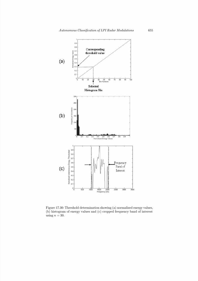
7/17/2019 1596932341 Intercept Radar.pdf
http://slidepdf.com/reader/full/1596932341-intercept-radarpdf 686/891
Autonomous Classi fi cation of LPI Radar Modulations 655
Figure 17.30: Threshold determination showing (a) normalized energy values,(b) histogram of energy values and (c) cropped frequency band of interestusing n = 30.

7/17/2019 1596932341 Intercept Radar.pdf
http://slidepdf.com/reader/full/1596932341-intercept-radarpdf 687/891
656 Detecting and Classifying LPI Radar
Figure 17.31: (a) LPF output, (b) cropped region, and (c) contour plot of the cropped region showing the Frank modulation.
range of values for each detection technique and each network. The bin num-ber that provides the best Pcc is selected. Once the threshold is determined,the values of An below the threshold are set to zero. Then the beginning andending frequencies of the frequency band of interest are determined as shownin Figure 17.30(c). Using the lowest and highest frequency values from thefrequency band of interest the modulation energy can now be cropped fromthe image.
After the determination of the modulation band of interest the energy isautonomously cropped from the LPF output containing the noise filtered im-
age. The cropping was illustrated in Figure 17.31. Figure 17.31(a) shows theLPF output that is obtained previously, Figure 17.31(b) shows the croppedregion and Figure 17.31(c) shows the contour plot where the signal energycan easily be seen. Once the LPF output is cropped, the new image is resizedto 50 × 400 pixels for the PWVD and CWD images. The QMFB images areresized to 30 × 120 pixels. Resizing is done in order to obtain as much simi-larity as possible between the same modulation types. Following the resizingoperation the columns of the resized image are formed with the feature vectorof size 50× 400 = 20, 000 for PWVD and CWD images, and of size 30× 120 =3,600 for the QMFB images.
17.5.3 Principal Components Analysis
Principal components analysis (PCA) is mathematically defined as an or-thogonal linear transformation that transforms the data to a new coordinatesystem such that the greatest variance by any projection of the data comes to

7/17/2019 1596932341 Intercept Radar.pdf
http://slidepdf.com/reader/full/1596932341-intercept-radarpdf 688/891
Autonomous Classi fi cation of LPI Radar Modulations 657
lie on the first coordinate (called the first principal component), the secondgreatest variance on the second coordinate, and so on [36]. In other words,PCA is a rotation of the existing axes to new positions in the space definedby the original variables, where there is no correlation between the new vari-ables defined by the rotation. PCA is theoretically the optimum transformfor a given data set in least square terms. That is, the method projects thehigh-dimensional data vectors onto a lower dimensional space by using a pro-
jection which best represents the data in a mean square sense. Using PCAthe given data vector is represented as a linear combination of the eigenvec-tors obtained from the data covariance matrix. As a result, lower dimensionaldata vectors may be obtained by projecting the high-dimensional data vectorsonto a number of dominant eigenvectors [37].
PCA can be used for dimensionality reduction of the feature vector byretaining those characteristics of the cropped modulation that contributemost to its variance, by keeping lower-order principal components and ig-
noring higher-order ones. This assumes of course, that the low-order compo-nents contain the most important features of the LPI modulation within thecropped (and resized) T-F data. To facilitate the PCA, we form a trainingmatrix X as shown in Figure 17.32 where N is the length of the feature vec-tor and P is the number of training signals, which is 50 for our results. It isimportant to note that the mean has been subtracted from the data set.
The PCA maps the ensemble of P N-dimensional vectorsX =
x1, x2, · · · , x p
onto an ensemble of P D-dimensional vectors Y =
y1
, y2
, · · · , y p
where D < N using a linear projection. This linear projection
can be represented by a rectangular matrix A so that [37]
Y = AH X (17.28)
where A has orthogonal column vectors, i = 1, 2, · · · , P and H is the Her-mitian operation. The matrix A is selected as the P ×D matrix containing theD eigenvectors associated with the larger eigenvalues of the data covariancematrix XH X. With this choice of transformation matrix A, the transformeddata vectors Y have uncorrelated components.
The matrix X is obtained first to form the training data set. The featureextraction algorithm is applied to the images in the “Training” folder foreach detection technique. The cropped images are resized and a columnvector is formed to represent the signal modulation. These column vectorsare stacked together to form the training data set matrix. The mean of thetraining matrix is calculated column wise and the mean is subtracted fromthe training data set matrix giving the matrix X. This operation is illustratedin Figure 17.32 where P is the number of training signals which is 50 for this
example, and N is the length of the feature vectors. For PWVD and CWDX is of dimension 20,000 ×50 (50 training signals) and for the QMFB X isof dimension 3,600×50.
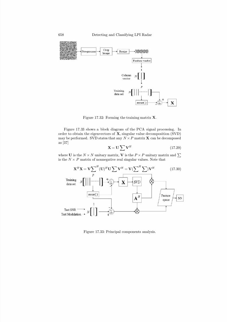
7/17/2019 1596932341 Intercept Radar.pdf
http://slidepdf.com/reader/full/1596932341-intercept-radarpdf 689/891
658 Detecting and Classifying LPI Radar
Figure 17.32: Forming the training matrix X.
Figure 17.33 shows a block diagram of the PCA signal processing. Inorder to obtain the eigenvectors of X, singular value decomposition (SVD)may be performed. SVD states that any N × P matrix X can be decomposedas [37]
X = U
VH (17.29)
where U is the N × N unitary matrix, V is the P × P unitary matrix and
is the N × P matrix of nonnegative real singular values. Note that
XH
X = VH (U)H
UVH
= V(H )VH
(17.30)
Figure 17.33: Principal components analysis.

7/17/2019 1596932341 Intercept Radar.pdf
http://slidepdf.com/reader/full/1596932341-intercept-radarpdf 690/891
Autonomous Classi fi cation of LPI Radar Modulations 659
indicates that the eigenvectors of XH X are contained in the V matrix andthe eigenvalues of XH X are the squared singular values of X, which are thediagonal elements of the matrix H . It can similarly be shown that theeigenvectors of XXH are contained in the U matrix.
If p = min(P, N ), both XXH and XH X will have the same p nonzeroeigenvalues. The product of X and V gives
XV = U
VH V = U
(17.31)
since V is unitary and the eigenvectors associated with nonzero eigenvaluescan be extracted by
U = XV−1
(17.32)
As a result, the nonzero eigenvalues of the higher dimensional covariancematrix XXH may be computed by computing the SVD of the smaller dimen-sional covariance matrix XH X.
Following the SVD of the data matrix and determination of the eigenvectormatrix U, dimensionality reduction is performed using the projection (trans-formation) matrix A. The matrix A is composed of D eigenvectors selectedfrom the eigenvector matrix U corresponding to D largest eigenvalues. In or-der to find the D largest eigenvalues, the biggest eigenvalue is multiplied by athreshold constant and the eigenvalues above the product are taken. Let T hλbe the eigenvalue selection threshold constant. In our example, three valuesare used as T hλ = [0.001, 0.005, 0.01]. For each case, once the eigenvalues arefound, four variations of eigenvector selection are used. Let these variationsbe ∨i, where i = 0, 1, 2, 3. The variations are defined by the i index as follows:
• ∨0: All the eigenvectors corresponding to the eigenvalues above T hλ are
used to form the matrix A.
• ∨1: All the eigenvectors corresponding to the eigenvalues above T hλ areselected initially; all of them except the eigenvector corresponding tothe eigenvalue with the highest value are used to form the matrix A.
• ∨2: All the eigenvectors corresponding to the eigenvalues above T hλ areselected initially; all of them except the two eigenvectors correspondingto the two eigenvalues with the highest values are used to form the ma-trix A.
• ∨3: All the eigenvectors corresponding to the eigenvalues above T hλ areselected initially; all of them except the three eigenvectors correspond-ing to the three eigenvalues with the highest values are used to form

7/17/2019 1596932341 Intercept Radar.pdf
http://slidepdf.com/reader/full/1596932341-intercept-radarpdf 691/891
660 Detecting and Classifying LPI Radar
the matrix A.
Once the projection matrix A is generated, both the training matrix Xand the test signals are projected onto a smaller dimensional feature space.The dataset is reduced in dimension to D using the projection process. Theprojected data is then used for classification.
17.5.4 Classification Using Modified Feature Extraction
The classification results in this section use an extended database to determinethe performance of the modified feature extraction technique as a functionof the SNR. After the database is described, steps to optimize the MLPand RBF are discussed. Classification results are then shown for both theTestSNR signals (same signals used in training but with varying SNR) andthe TestMod signals (diff erent modulations and varying SNR).
Extended Database
To investigate the detailed performance of the modified feature extraction andclassification process, a more extensive database is developed that consists of 12 LPI modulation techniques each having 21 SNR levels(−10 dB, −9 dB, · · · ,9 dB, 10 dB). The LPI modulation techniques includeCostas frequency hopping, Costas frequency hopping plus a Barker phaseshift keying, FMCW, PSK and FSK. PSK signals include polyphase (Frank,P1, P2, P3, P4) and polytime (T1, T2, T3, T4) codes. This database allowsa detailed look at the Pcc as a function of the SNR. The signals are generatedusing the LPIT and placed in the “Input” folder within the proper subfolder(TestSNR, TestMod, Training, Signals). Note that the “Signals” folder should
contain only one signal from each modulation type being used. This folderis used to correlate the modulation prefix (F for FMCW, FR for Frank andso forth) to build the confusion matrix. The output T-F and B-F imagesfrom the detection signal processing (Wigner-Ville, Choi-Williams, quadra-ture mirror filtering, cyclostationary processing) are automatically placed inthe corresponding output folder (e.g., QMFB output). Before the feature ex-traction and nonlinear classification signal processing algorithms are run, thedetection output signals within the “TestMod” and “TestSNR” folders thathave the same SNR must be collected and put into a folder that designatesthe SNR (e.g., TestMod-10, and TestSNR4). The folder structure should beas shown in Figure 17.34. Note that the SNR = 10 dB signals for each modu-lation are used for training. This is a choice that the user can make. Trainingthe LPI feature extraction and classification networks with only “signal only”
waveforms however, is not realistic since any received signal will have a noisecomponent related to the thermal noise present in the intercept receiver andthe range of the LPI emitter.

7/17/2019 1596932341 Intercept Radar.pdf
http://slidepdf.com/reader/full/1596932341-intercept-radarpdf 692/891
Autonomous Classi fi cation of LPI Radar Modulations 661
Figure 17.34: Folder structure for TestSNR, TestMod, and Training (10-dBTestSNR only) [32].
Table 17.9: Costas Frequency Hopping Modulation Parameters for TestSNR(f s = 7,000 Hz)
Signal Frequency Frequencymodulation sequence (Hz) duration tp (ms)Costas 3, 2, 6, 4, 5, 1 × 200 5
2, 4, 8, 5, 10, 9, 7, 3, 6, 1 × 150 3
Signals Used for TestSNR and TestMod
The signals used to test the performance of the feature extraction and clas-sification signal processing for various values of SNR are described below.
This database is used to generate the results shown in this section. Super-vised training of the autonomous classification process is done with the signalmodulations below using SNR = 10 dB. The parameters for the Costas codesand the Costas codes with a Barker PSK used for testing the performanceof the classification signal processing as a function of the SNR are shown inTables 17.9 and 17.10, respectively. The FMCW signal parameters are shownin Table 17.11. The polyphase signals (Frank, P1—P4) used for testing theperformance as a function of the SNR are as shown in Table 17.12. Tables17.13 and 17.14 are the polytime signals T1, T2, T3, and T4 respectively.These signals are used to evaluate the performance of the autonomous clas-sification Pcc when the received signal has the same modulation parametersbut diff erent SNR.
After supervised training of the classification network using the
SNR = 10 dB signals from the TestSNR database, the performance usingthe signals from the TestMod database are evaluated. It is important to

7/17/2019 1596932341 Intercept Radar.pdf
http://slidepdf.com/reader/full/1596932341-intercept-radarpdf 693/891
662 Detecting and Classifying LPI Radar
Table 17.10: Costas Plus Barker PSK Frequency Hopping ModulationParameters for TestSNR (f s = 7,000 Hz)
Signal Frequency Barker subcodemodulation sequence (Hz) period tb (ms)Costas + PSK 3, 2, 6, 4, 5, 1 × 150 1 (N c = 5)
5, 4, 6, 2, 3, 1 × 300 0.3 (N c = 13)
Table 17.11: FMCW Modulation Parameters for TestSNR
Signal Carrier Modulation Modulationmodulation frequency bandwidth period
f c (Hz) ∆F (Hz) tm (ms)
FMCW 1,495 250 15
2,195 800 15
point out that this is a more difficult (and realistic) situation. The TestModsignals model the interception of a waveform with a modulation that is notwithin the training set. The signals in TestMod are also tested as a functionof the SNR. The Costas frequency hopping modulation parameters and theCostas frequency hopping plus Barker PSK modulation parameters used forTestMod are shown in Tables 17.15 and 17.16, respectively. The FMCW sig-nals used for testing the performance of the signal processing as a function of the SNR are as shown in Table 17.17. The polyphase signals (Frank, P1—P4)used for testing the performance as a function of the SNR are as shown inTable 17.18. The polytime signals are shown in Tables 17.19 and 17.20.
Optimizing the Feature Extraction and Classification Network
Using the initial nonlinear network parameters two feature extractionparameters, LPF cutoff frequency and histogram bin, must be optimized.Using the optimum values derived, the PCA network parameters are thenoptimized. The Pcc results shown are with the final optimum values. Theoptimization is performed using the test signals with SNR = 10 dB. Theoptimum parameter selection is based on the highest average Pcc.
For each detection technique, the MLP network configuration starts witha default set of values for the epochs, the number of neurons in the first andsecond hidden layers S 1, S 2, the eigenvalue selection threshold constant T hλand eigenvector selection variations ∨i. Once the initial values are set, anoptimization is performed to determine optimum values for the LPF digitalfrequencies ω1 = ω2 and histogram bin number. After these two values are
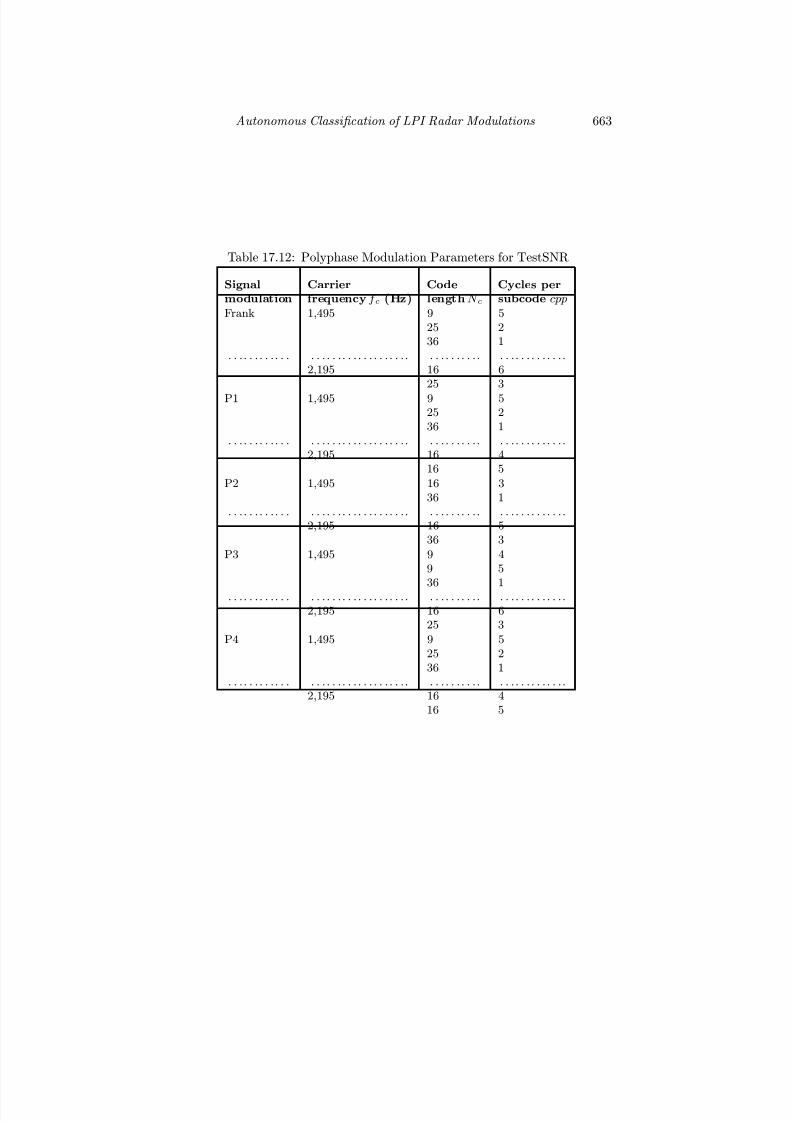
7/17/2019 1596932341 Intercept Radar.pdf
http://slidepdf.com/reader/full/1596932341-intercept-radarpdf 694/891
Autonomous Classi fi cation of LPI Radar Modulations 663
Table 17.12: Polyphase Modulation Parameters for TestSNR
Signal Carrier Code Cycles permodulation frequency f c (Hz) length N c subcode cpp
Frank 1,495 9 525 236 1
. . . . . . . . . . . . . . . . . . . . . . . . . . . . . . . . . . . . . . . . . . . . . . . . . . . . . .2,195 16 6
25 3
P1 1,495 9 525 236 1
. . . . . . . . . . . . . . . . . . . . . . . . . . . . . . . . . . . . . . . . . . . . . . . . . . . . . .2,195 16 4
16 5
P2 1,495 16 336 1
. . . . . . . . . . . . . . . . . . . . . . . . . . . . . . . . . . . . . . . . . . . . . . . . . . . . . .2,195 16 5
36 3
P3 1,495 9 49 536 1
. . . . . . . . . . . . . . . . . . . . . . . . . . . . . . . . . . . . . . . . . . . . . . . . . . . . . .2,195 16 6
25 3
P4 1,495 9 525 236 1
. . . . . . . . . . . . . . . . . . . . . . . . . . . . . . . . . . . . . . . . . . . . . . . . . . . . . .2,195 16 4
16 5

7/17/2019 1596932341 Intercept Radar.pdf
http://slidepdf.com/reader/full/1596932341-intercept-radarpdf 695/891
664 Detecting and Classifying LPI Radar
Table 17.13: Polytime T1, T2 Modulation Parameters for TestSNR
Signal Carrier Code No. phase No. codemodulation frequency period states segments
f c (Hz) T (ms) n k
T1 1,495 30 2 530 3 4
. . . . . . . . . . . . . . . . . . . . . . . . . . . . . . . . . . . . . . . . . . . . . . . . . . .2,195 30 2 3
30 2 430 4 3
T2 1,495 30 4 330 8 4
. . . . . . . . . . . . . . . . . . . . . . . . . . . . . . . . . . . . . . . . . . . . . . . . . . .2,194 30 4 3
30 4 4
30 6 3
Table 17.14: Polytime T3, T4 Modulation Parameters for TestSNR
Signal Carrier Modulation Modulation No. phasemodulation frequency period bandwidth states
f c (Hz) tm (ms) ∆F (Hz) n
T3 1,495 25 300 430 900 9
. . . . . . . . . . . . . . . . . . . . . . . . . . . . . . . . . . . . . . . . . . . . . . . . . . . . . . . . . . . .2,195 25 400 2
30 1000 7
35 800 6T4 1,495 25 400 2
30 550 330 850 7
. . . . . . . . . . . . . . . . . . . . . . . . . . . . . . . . . . . . . . . . . . . . . . . . . . . . . . . . . . . .2,194 30 600 5
30 900 9
Table 17.15: Costas Frequency Hopping Modulation Parameters for TestMod(f s = 7,000 Hz)
Signal Frequency Frequency
modulation sequence (Hz) duration tp (ms)Costas 5, 4, 6, 2, 3, 1 × 400 5

7/17/2019 1596932341 Intercept Radar.pdf
http://slidepdf.com/reader/full/1596932341-intercept-radarpdf 696/891
Autonomous Classi fi cation of LPI Radar Modulations 665
Table 17.16: Costas Plus Barker PSK Frequency Hopping Modulation
Parameters for TestMod (f s = 7,000 Hz)
Signal Frequency Barker subcodemodulation sequence (Hz) period tb (ms)Costas + PSK 3, 2, 6, 4, 5, 1 × 200 0.4 (N c = 11)
5, 4, 6, 2, 3, 1 × 250 0.7 (N c = 7)
Table 17.17: FMCW Modulation Parameters for TestMod
Signal Carrier Modulation Modulationmodulation frequency bandwidth period
f c (Hz) ∆F (Hz) tm (ms)
FMCW 1,495 500 202,195 400 20
Table 17.18: Polyphase Modulation Parameters for TestMod
Signal Carrier Code Cycles permodulation frequency f c (Hz) length N c subcode cpp
Frank 1, 495 9 4. . . . . . . . . . . . . . . . . . . . . . . . . . . . . . . . . . . . . . . . . . . . . . . . . . . . . .
2, 195 16 416 5
P1 1,495 9 4. . . . . . . . . . . . . . . . . . . . . . . . . . . . . . . . . . . . . . . . . . . . . . . . . . . . . .
2,195 16 625 3
P2 1,495 16 2. . . . . . . . . . . . . . . . . . . . . . . . . . . . . . . . . . . . . . . . . . . . . . . . . . . . . .
2,195 16 4
P3 1,495 25 2. . . . . . . . . . . . . . . . . . . . . . . . . . . . . . . . . . . . . . . . . . . . . . . . . . . . . .
2,195 16 416 5
P4 1,495 9 4. . . . . . . . . . . . . . . . . . . . . . . . . . . . . . . . . . . . . . . . . . . . . . . . . . . . . .
2,195 16 625 3

7/17/2019 1596932341 Intercept Radar.pdf
http://slidepdf.com/reader/full/1596932341-intercept-radarpdf 697/891
666 Detecting and Classifying LPI Radar
Table 17.19: Polytime T1, T2 Modulation Parameters for TestMod
Signal Carrier Code No. phase No. codemodulation frequency period states segments
f c (Hz) T (ms) n k
T1 1,495 30 4 430 6 3
. . . . . . . . . . . . . . . . . . . . . . . . . . . . . . . . . . . . . . . . . . . . . . . . . . .2,195 30 3 3
T2 1,495 30 6 430 4 5
. . . . . . . . . . . . . . . . . . . . . . . . . . . . . . . . . . . . . . . . . . . . . . . . . . .
2, 194 30 8 3
Table 17.20: Polytime T3, T4 Modulation Parameters for TestMod
Signal Carrier Modulation Modulation No. phasemodulation frequency period bandwidth states
f c (Hz) tm (ms) ∆F (Hz) n
T3 1,495 30 500 535 700 8
. . . . . . . . . . . . . . . . . . . . . . . . . . . . . . . . . . . . . . . . . . . . . . . . . . . . . . . . . . . .2,195 30 600 3
T4 1,495 35 700 6. . . . . . . . . . . . . . . . . . . . . . . . . . . . . . . . . . . . . . . . . . . . . . . . . . . . . . . . . . . .
2,194 25 450 435 750 8

7/17/2019 1596932341 Intercept Radar.pdf
http://slidepdf.com/reader/full/1596932341-intercept-radarpdf 698/891
Autonomous Classi fi cation of LPI Radar Modulations 667
Table 17.21: Optimum Feature Extraction and MLP Parameters
Detection ω1 = ω2 Bin S 1 = S 2 T hλ ∨i epochsWigner-Ville 0.1π 45 80 0.001 ∨1 5,000Choi-Williams 0.1π 15 80 0.001 ∨0 6,000
Quadrature mirror 0.4π 18 60 0.005 ∨0 5,000
Table 17.22: Optimum Feature Extraction and RBF Parameters
Detection ω1 = ω2 Bin σ goal T hλ ∨i
Wigner-Ville 0.2π 55 2000 0.9 0.001 ∨0
Choi-Williams 0.5π 55 3500 0.9 0.001 ∨0
Quadrature mirror 0.6π 4 25 0.8 0.001 ∨0
found, a second optimization for epochs, S 1, S 2, T hλ and ∨i is performed.Once all the values are found and set the classification network is tested. Forthe classification of PWVD images the initial values used are epochs = 6,000S 1 = S 2 = 50, T hλ = 0.001 and ∨i = ∨0. After optimization ω1 = ω2 = 0.1πand the histogram bin number is 45. Using these values, the remaining para-meters giving optimum Pcc are S 1 = S 2 = 80, T hλ = 0.001, ∨1 and epochs =5,000. The optimization is repeated for the Choi-Williams, the quadraturemirror filtering, and the Wigner-Ville distribution detection techniques. Ta-ble 17.21 shows the resulting optimum parameters using the MLP. A similaroptimization is also run for the RBF. The optimum parameters are shown inTable 17.22 for the RBF.
17.5.5 Classification Results with the Multilayer
Perceptron
The classification results are presented for comparison of the three T-F detec-tion techniques including the Choi-Williams distribution (CWD), the pseudoWigner-Ville distribution (PWVD) and the quadrature mirror filter bankapproach (QMFB). The MLP classification results for the Costas frequencyhopping code are shown in Figure 17.35 and the results for the Costas plusBarker PSK are shown in Figure 17.36. The MLP classification results for theFMCW are shown in Figure 17.37. The MLP results for the Frank, P1—P4,T1—T4 are shown in Figures 17.38—17.46.
All the detection techniques show similar results on the TestSNR case.
Most of the modulations are classified with more than 80% classification ratefor SNR > 0 dB. There is a considerable stability in classification of signalswith SNR > 0 dB. This stability indicates that the autonomous modulation

7/17/2019 1596932341 Intercept Radar.pdf
http://slidepdf.com/reader/full/1596932341-intercept-radarpdf 699/891
668 Detecting and Classifying LPI Radar
Figure 17.35: Costas code classification results using the MLP for (a) Test-SNR and (b) TestMod.
Figure 17.36: Costas frequency hopping plus PSK classification results usingthe MLP for (a) TestSNR and (b) TestMod.

7/17/2019 1596932341 Intercept Radar.pdf
http://slidepdf.com/reader/full/1596932341-intercept-radarpdf 700/891
Autonomous Classi fi cation of LPI Radar Modulations 669
Figure 17.37: FMCW classification results using the MLP for (a) TestSNRand (b) TestMod.
Figure 17.38: Frank classification results using the MLP for (a) TestSNR and(b) TestMod.
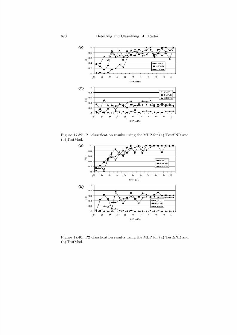
7/17/2019 1596932341 Intercept Radar.pdf
http://slidepdf.com/reader/full/1596932341-intercept-radarpdf 701/891
670 Detecting and Classifying LPI Radar
Figure 17.39: P1 classification results using the MLP for (a) TestSNR and(b) TestMod.
Figure 17.40: P2 classification results using the MLP for (a) TestSNR and(b) TestMod.
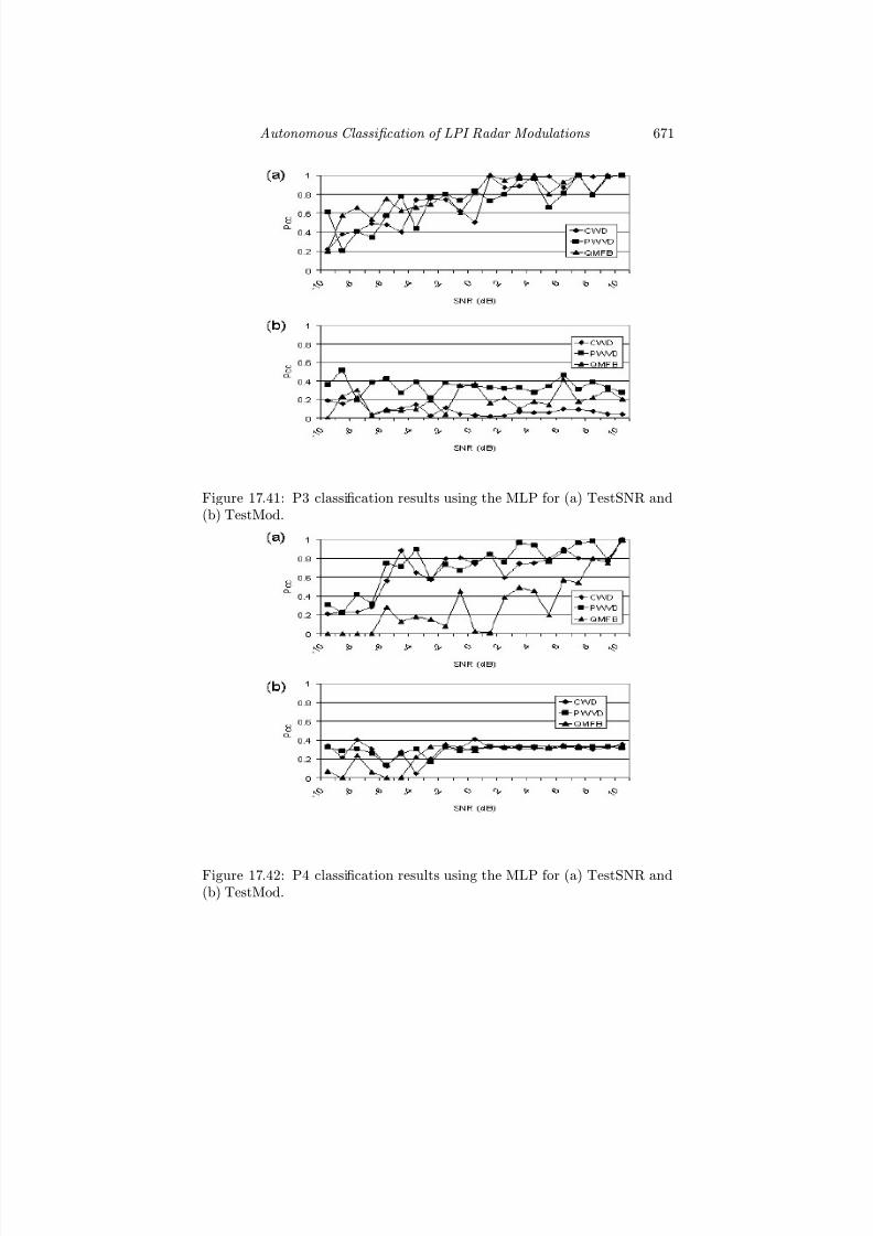
7/17/2019 1596932341 Intercept Radar.pdf
http://slidepdf.com/reader/full/1596932341-intercept-radarpdf 702/891
Autonomous Classi fi cation of LPI Radar Modulations 671
Figure 17.41: P3 classification results using the MLP for (a) TestSNR and(b) TestMod.
Figure 17.42: P4 classification results using the MLP for (a) TestSNR and(b) TestMod.

7/17/2019 1596932341 Intercept Radar.pdf
http://slidepdf.com/reader/full/1596932341-intercept-radarpdf 703/891
672 Detecting and Classifying LPI Radar
Figure 17.43: T1 classification results using the MLP for (a) TestSNR and(b) TestMod.
Figure 17.44: T2 classification results using the MLP for (a) TestSNR and(b) TestMod.

7/17/2019 1596932341 Intercept Radar.pdf
http://slidepdf.com/reader/full/1596932341-intercept-radarpdf 704/891
Autonomous Classi fi cation of LPI Radar Modulations 673
Figure 17.45: T3 classification results using the MLP for (a) TestSNR and(b) TestMod.
Figure 17.46: T4 classification results using the MLP for (a) TestSNR and(b) TestMod.

7/17/2019 1596932341 Intercept Radar.pdf
http://slidepdf.com/reader/full/1596932341-intercept-radarpdf 705/891
674 Detecting and Classifying LPI Radar
energy isolation and cropping becomes more sensitive to noise variations be-low 0 dB. The Pcc of Frank, FSK/PSK, FMCW, T1, T2, and T4 modulationswith PWVD and CWD techniques exhibit 100% for most of the SNR levelsabove 0 dB.
Concerning the TestMod case, the best results are obtained in the clas-sification of FMCW, Costas, FSK/PSK, P2, and T2 modulations while theworst results are obtained in the classification of polyphase codes. Note thatmost of the results for Frank, P1, P3, and P4 modulations are below Pcc =0.4. Classification of Costas, FSK/PSK, FMCW, P2, P4, T1, T2, T3, andT4 modulations with PWVD and CWD techniques exhibit similar results.Overall, the classification results with the PWVD technique outperform theother detection techniques. Overall the QMFB technique performs worsethan the other techniques but it does well in the classification of T2 and T4modulations for SNR > 5 dB. Recall that the QMFB images have a verylow resolution compared to the PWVD and CWD images, which becomes a
disadvantage for modulation discrimination.One interesting result is observed on Costas modulation classification.While the Pcc for TestMod is 100% with all detection techniques, the Pccfor TestSNR is not. This is an unexpected result. It is expected that theTestSNR results would outperform the TestMod results since the signals usedin TestSNR have the same parameters as the training signals. In this sensethe TestSNR results can be used as a measure of reliability. This showsthat, although the Costas results seem very good for TestMod case, theymay not be reliable. Further, it is shown that the classification of Costascode is best performed with CWD detection technique for SNR > 4 dB.Note also that it is not necessarily true that the TestMod results performbetter if the TestSNR results perform well. The Pcc for TestMod dependson the modulation discriminative power of the feature extraction algorithm
implemented.
17.5.6 Classification Results with the Radial Basis
Function
The RBF classification results for the Costas frequency hopping signals areshown in Figure 17.47. The RBF classification results for the Costas plusPSK frequency hopping signals are shown in Figure 17.48. The results forthe FMCW signals are shown in Figure 17.49. The results for the Frankpolyphase signals are shown in Figure 17.50. The RBF classification resultsfor the P1—P4 polyphase signals are shown in Figures 17.51—17.54. The resultsfor the T1 and T2 polytime signals are shown in Figures 17.55—17.58.
For the TestSNR classification, the Frank, FMCW, P2, T1, T2, T3 and T4
modulations are classified with greater than Pcc = 80% probability of correctclassification for SNR > 2 dB. The autonomous modulation energy isolationand cropping becomes more sensitive to noise variations below SNR = 2 dB.

7/17/2019 1596932341 Intercept Radar.pdf
http://slidepdf.com/reader/full/1596932341-intercept-radarpdf 706/891
Autonomous Classi fi cation of LPI Radar Modulations 675
Figure 17.47: Costas classification results using the RBF for (a) TestSNR and(b) TestMod.
The FMCW modulation is classified with 100% for SNR > 4 dB, and theP2 modulation is classified with 100% for SNR > 4 dB with all detectiontechniques.
Concerning the TestMod case, the best results are obtained in the clas-sification of FMCW, Costas, P1, P2 and T2 modulations while the worstresults are obtained in the classification of P4, T1 and T3 modulations. TheFMCW modulation is classified 100% with PWVD detection technique forSNR > −10 dB and 100% with CWD detection technique for SNR > −1 dB .The T4 modulation is classified 100% with PWVD detection for SNR > 2 dBand the P2 modulation is classified 100% with CWD detection for SNR > −3dB. Overall, the classification results with the PWVD technique outperformthe other detection techniques. The QMFB technique performs worse thanthe other two detection techniques. It outperforms however, the other tech-niques in the classification of the P1 modulation with a Pcc above 66%.
MLP and RBF Comparision
Both the MLP and RBF networks are examples of nonlinear layered feedfor-ward networks. The important trait that is illustrated in the figures shown
is that the RBF classification Pcc results are not as stationary as those forthe MLP. This is due in part to the fact that the RBF has a single hidden

7/17/2019 1596932341 Intercept Radar.pdf
http://slidepdf.com/reader/full/1596932341-intercept-radarpdf 707/891
676 Detecting and Classifying LPI Radar
Figure 17.48: Costas plus PSK classification results using the RBF for(a) TestSNR and (b) TestMod.
Figure 17.49: FMCW classification results using the RBF for (a) TestSNRand (b) TestMod.

7/17/2019 1596932341 Intercept Radar.pdf
http://slidepdf.com/reader/full/1596932341-intercept-radarpdf 708/891
Autonomous Classi fi cation of LPI Radar Modulations 677
Figure 17.50: Frank classification results using the RBF for (a) TestSNR and(b) TestMod.
Figure 17.51: P1 classification results using the RBF for (a) TestSNR and(b) TestMod.
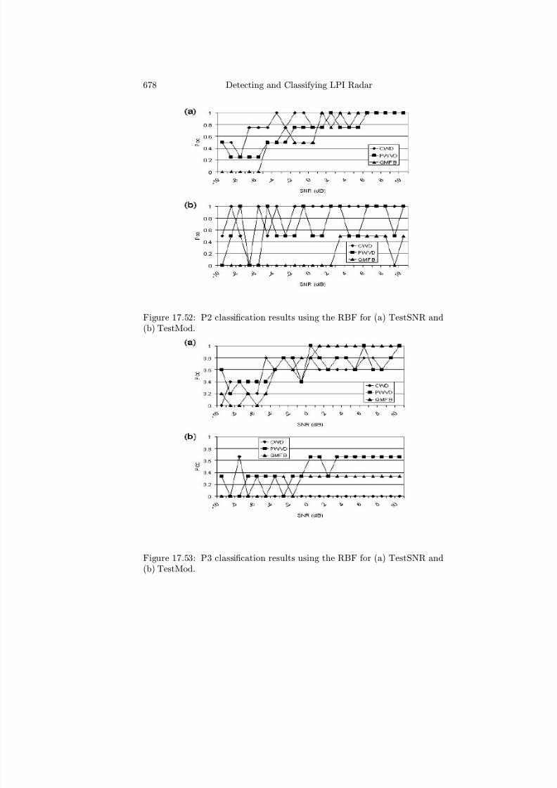
7/17/2019 1596932341 Intercept Radar.pdf
http://slidepdf.com/reader/full/1596932341-intercept-radarpdf 709/891
678 Detecting and Classifying LPI Radar
Figure 17.52: P2 classification results using the RBF for (a) TestSNR and(b) TestMod.
Figure 17.53: P3 classification results using the RBF for (a) TestSNR and(b) TestMod.

7/17/2019 1596932341 Intercept Radar.pdf
http://slidepdf.com/reader/full/1596932341-intercept-radarpdf 710/891
Autonomous Classi fi cation of LPI Radar Modulations 679
Figure 17.54: P4 classification results using the RBF for (a) TestSNR and(b) TestMod.
Figure 17.55: T1 classification results using the RBF for (a) TestSNR and(b) TestMod.

7/17/2019 1596932341 Intercept Radar.pdf
http://slidepdf.com/reader/full/1596932341-intercept-radarpdf 711/891
680 Detecting and Classifying LPI Radar
Figure 17.56: T2 classification results using the RBF for (a) TestSNR and(b) TestMod.
Figure 17.57: T3 classification results using the RBF for (a) TestSNR and(b) TestMod.

7/17/2019 1596932341 Intercept Radar.pdf
http://slidepdf.com/reader/full/1596932341-intercept-radarpdf 712/891
Autonomous Classi fi cation of LPI Radar Modulations 681
Figure 17.58: T4 classification results using the RBF for (a) TestSNR and(b) TestMod.
layer, whereas the MLP has two hidden layers. Also, the computation nodesof the MLP within a hidden or output layer share a common neuronal modelwhereas the computation nodes in the hidden layer of the RBF network havea significantly diff erent purpose from those in the output layer of the network.The argument of the activation function of each hidden unit in the RBF net-work computes the Euclidean norm (distance) between the input vector andthe center of that unit. For the MLP the activation function of each hid-den unit computes the inner product of the input vector and the synapticweight vector of that unit. Finally, the MLP constructs a global approxima-tion to the nonlinear input-output mapping of the LPI modulations while theRBF network uses exponentially decaying localized nonlinearities (Gaussianfunctions) to construct local approximations to the nonlinear input-outputmappings. For the approximation of a nonlinear input-output mapping, theMLP requires a smaller number of parameters than the RBF network for thesame degree of accuracy [23].
7/17/2019 1596932341 Intercept Radar.pdf
http://slidepdf.com/reader/full/1596932341-intercept-radarpdf 713/891
682 Detecting and Classifying LPI Radar
17.6 Summary
Autonomous (no human operator intervention) feature extraction and classifi-
cation algorithms that can be used for identification of LPI radar modulationsusing time-frequency (T-F) images are presented. The first approach uses ahistogram processing of the marginal frequency distribution to identify themodulation within the T-F image. After the modulation is cropped from theimage, an adaptive binarization process is used to develop a feature vectorfor classification of the modulation contained in the signal. Classificationtechniques evaluated include the multilayer perceptron and the radial basisfunction neural networks. To evaluate the performance of the feature ex-traction processing, the classification results for five LPI modulations wereinvestigated. The algorithms were trained using an SNR = 10 dB. To eval-uate the classification performance of the algorithms, a database containingthe LPI signals with varying SNR was used (TestSNR database). A seconddatabase containing the same modulations but with varied parameters (Test-Mod database) was also used. The percent of correctly classified modulationsfor this considerably more difficult (but more realistic) database set of signals,were much lower than the TestSNR signals.
Due to the poor stability of the cropping region and the large size of thefeature vector, a modified feature extraction method was also presented. Themodified approach included the addition of a filtering process (to reduce thepresence of high frequency noise) and the use of principal components analysis(to reduce the dimensionality). Results showed good improvement and theperformance of the modified feature extraction technique was evaluated as afunction of SNR. Both the TestSNR and TestMod results were shown. Byeliminating the need for a human operator to examine the T-F results, real-time signal analysis is possible, which can allow a faster response management
to the intercepted threat signals.
References
[1] Azzouz, E., and Nandi, A. K., Automatic Modulation Recognition of Com-munication Signals , Kluwer Academic Publishers, 1996.
[2] Nandi, A. K., and Azzouz, E., “Algorithms for automatic modulation recog-nition of communication signals,” IEEE Trans. on Communications, Vol. 46,No. 4, pp. 431—436, April 1998.
[3] Azzouz, E., and Nandi, A. K., “Automatic identification of digital modulationtypes,” Signal Processing , Vol. 47, No. 1, pp. 55—69, 1995.
[4] Louis, C., and Sehier, P. “Automatic modulation recognition with a hierar-
chical neural network,” Record of the IEEE Military Communications Con- ference, MILCOM ’94, Vol. 3, pp. 713—717, October 1994.

7/17/2019 1596932341 Intercept Radar.pdf
http://slidepdf.com/reader/full/1596932341-intercept-radarpdf 714/891
Autonomous Classi fi cation of LPI Radar Modulations 683
[5] Lin, Y-C., and Kuo, C-C. J., “Modulation classification using wavelet trans-form,” Proc. of the SPIE, Vol. 2303, pp. 260—271, Wavelet Applications inSignal and Image Processing II, Andrew F. Laine, Michael A. Unser; Eds.,
Oct. 1994.
[6] Reichert, J., “Automatic classification of communication signals using higherorder statistics,” Proc. of the IEEE International Conference on Acoustics,Speech and Signal Processing , Vol. 5, pp. 221—224, 23—26 Mar. 1992.
[7] Schreyogg, C., Kittel, K., Kressel, U., and Reichert, J., “Robust classificationof modulation types using spectral features applied to HMM,” Record of the IEEE Military Communications Conference, MILCOM ’97 , Vol. 3, pp. 1377—1381, Nov. 1997.
[8] Breakenridge, C. “Nonstationary signal classification using time-frequencyoptimization,” Proc. of the 10th IEEE International Conference on Electron-ics, Circuits and Systems, ICECS , pp. 132—135, 14—17 Dec. 2003,
[9] Roberts, G., Zoubir, A. M., and Boashash, B., “Time-frequency classifica-
tion using a multiple hypothesis test: an application to the classifi
cation of humpback whale signals,” Proc. of the IEEE International Conference on Acoustics, Speech, and Signal Processing , Vol. 1, pp. 563—566, 1997.
[10] Breakenridge, C., and Mesbah, M., “Minimum classification error using time-frequency analysis,” Proc. of the 3rd IEEE International Symposium on Sig-nal Processing and Information Technology, ISSPIT , pp. 717—720, 14—17 Dec.2003.
[11] Wang, T. Deng, J., and He, B., “Classification of motor imagery EEG pat-terns and their topographic representation,” Proc. of the International Con- ference on Engineering in Medicine and Biology Society, IEMBS ’04, pp.4359—4362, 1—5 Sept. 2004.
[12] Gache, N., Chevret, P., and Zimpfer, V., “Target classification near complexinterfaces using time-frequency filters,” Proceedings of the IEEE International
Conference on Acoustics, Speech and Signal Processing , Vol. 4, pp. 2433—2436, 12—15 May 1998.
[13] Kim, K.-T., Choi, I.-S., and Kim, H.-T., “Efficient radar target classificationusing adaptive joint time-frequency processing,” IEEE Trans. on Antennas and Propagation , Vol. 48, No. 12, pp. 1789—1801, Dec. 2000.
[14] Chilukuri, M. V., Dash, P. K., and Basu, K. P., “Time-frequency based pat-tern recognition technique for detection and classification of power qualitydisturbances,” Proc. of the IEEE Region 10 Conference, Vol. 3, pp. 260—263, 21—24 Nov. 2004.
[15] Gillespie, B. W., and Atlas, L. E., “Optimizing time-frequency kernels forclassification,” IEEE Trans. on Signal Processing, Vol. 49, No. 3, pp. 485—496, March 2001.
[16] Shelton, C. P., “Human Interface/Human Error,” em Dependable EmbeddedSystems, Carnegie Mellon University pp. 18—849b Spring 1999.
7/17/2019 1596932341 Intercept Radar.pdf
http://slidepdf.com/reader/full/1596932341-intercept-radarpdf 715/891
684 Detecting and Classifying LPI Radar
[17] De vries, M. F. L., Koeners, G. J. M., Roefs, F. D., Van ginkel, H. T. A.,and Theunissen, E., “Operator Support for Time-Critical Situations: Designand Evaluation,” Proc. of the IEEE/AIAA 25th Digital Avionics Systems
Conference , Delft Univ. of Tech., Netherlands, pp. 1—14, Oct. 2006.
[18] Sheridan, T. B., Humans and Automation: System Design and Research Is-sues , John Wiley & Sons, Inc., 2002.
[19] Upperman, G. J., Upperman, T. L., Fouts, D. J., and Pace, P. E., “Efficienttime-frequency and bi-frequency signal processing on a reconfigurable com-puter,” IEEE Asilomar Conference on Signals, Systems and Computers , Nov.2008.
[20] Lippmann, R. P., “An introduction to computing with neural nets,” IEEE ASSP Magazine , pp. 4—22, April 1987.
[21] Hush, D. R., and Horne, B. G., “Progress in supervised neural networks,”IEEE Signal Processing Magazine , pp. 8—39, Jan. 1993.
[22] Wong, M. L. D., and Nandi, A. K., “Automatic digital modulation recognition
using artificial neural network and genetic algorithm,” Signal Processing, Vol.84, No. 2, pp. 351—365, February 2004.
[23] Haykin, S., Neural Networks—A Comprehensive Foundation, Second Ed., Up-per Saddle River, New Jersey: Prentice Hall, 1999.
[24] Theodoridis, S., and Koutroumbas, K., Pattern Recognition, Third Ed., SanDiego, CA: Academic Press, 2006.
[25] Broomhead, D. S., and Low, D., “Multi-variate functional interpolation andadaptive networks,” Complex Systems , Vol. 2, pp. 321—355, 1990.
[26] Husain, H., Khalid, M., and Yusof, R., “Nonlinear function approximationusing radial basis function neural networks,” Student Conference on Research and Development , pp. 326—329, July 2002.
[27] Atlas, L., Owsley, L., McLaughlin, J., and Bernard, G., “Automatic feature-
finding for time-frequency distributions,” Proceedings of the IEEE-SP Inter-national Symposium on Time-Frequency and Time-Scale Analysis , pp. 333—336, 18—21 June 1996.
[28] Zilberman, E. R., and Pace, P. E., “Autonomous time-frequency morpho-logical feature extraction algorithm for LPI radar modulation classification,”Proc. of the IEEE International Conf. on Image Processing , 2006.
[29] Cohen, L., “Time-frequency distributions—A review,” Proc. of the IEEE , Vol.77, No. 7, p. 941—981, 1989.
[30] Zilberman, E. R., and Pace, P. E., “Autonomous cropping and featureextraction using time-frequency marginal distributions for LPI radar clas-sification,” Proc. of the IASTED International Conf. on Signal and Image Processing , Aug., 2006.
[31] Van De Ville, D.,Van de Walle, R., Philips, W., and Lemahieu, I., “Imageresampling between orthogonal and hexagonal lattices,” Proc. International Conf. on Image Processing , Vol. 3, pp. III-389—III-392, 24—28 June 2002.

7/17/2019 1596932341 Intercept Radar.pdf
http://slidepdf.com/reader/full/1596932341-intercept-radarpdf 716/891
Autonomous Classi fi cation of LPI Radar Modulations 685
[32] Gulum, T. O., “Autonomous Non-Linear Classification of LPI Radar SignalModulations,” Naval Postgraduate School Master’s Thesis, 2007.
[33] Gonzales, R. C., Woods R. E. and Eddins, S. L., Digital Image Processing Using MATLAB , Upper Saddle River, NJ, Prentice Hall, 2004.
[33] Lim, J. S., Two-Dimensional Signal and Image Processing , Englewood Cliff s,NJ Prentice Hall, 1990.
[34] Oppenheim, A. V., Willsky, A. S., and Nawab, S. H., Signals and Systems,Upper Saddle River, NJ: Prentice Hall, 1997.
[35] Jolliff e, I. T., Principal Component Analysis, Series: Springer Series in Sta-tistics, 2nd ed., Springer, New York, 2002.
[36] Fargues, M. P., “Investigation of Feature dimension Reduction Schemes forClassification Applications,” Naval Postgraduate School Technical Report,Monterey, CA, NPS-EC-01-005, June 2001.
[37] Therrien, C. W., Discrete Random Signals and Statistical Signal Processing ,Prentice Hall, Englewood Cliff s, NJ, 1991.
Problems
1. Setting Up the Database:
a. Begin by reading the Readme.doc file in the LPI Class folder on theCD.
b. Using the LPIT, generate with a sampling frequency of f s = 7,000 Hz,and SNR = 10 dB, a BPSK signal, a polyphase Barker signal, a P1signal, a P2 signal, a P3 signal, a P4 signal, a Frank code signal, aFMCW signal, T1(2) and a T3(2) signal. Make sure you record the
parameters for each of your signals.c. Go to the Input Folder. The Input Folder should have four subfolders.
They are the Signals, TestSNR, TestMod and Training folders. Copythe 10 signals into the Training folder and the Signals Folder.
d. Copy the 10 signals into the TestSNR folder.
e. For each signal generated in b., generate the same signal but withSNR = −10,−9, . . . , 0, . . . , 8, 9 dB. Copy these signals into theTestSNR folder.
f. For each signal generated in b., generate the signal with diff erent mod-ulation parameters and SNR = −10,−9, . . . , 0, . . . , 10 dB. Be sure to
record the modulation parameters for each signal. Copy these signalsinto the input TestMod folder.
7/17/2019 1596932341 Intercept Radar.pdf
http://slidepdf.com/reader/full/1596932341-intercept-radarpdf 717/891
686 Detecting and Classifying LPI Radar
2. Running the Detection Signal Processing:
a. Go to the LPI class folder and examine and run the MATLAB script fileSCRIPT detection ALL.m. This runs the Wigner-Ville distribution,Choi-Williams distribution, quadrature mirror filtering, and cyclosta-tionary detection signal processing algorithms on all of the files withinthe Input folder database. Note that these detection algorithms may berun separately by commenting out all but one of the detection process-ing calls. The output files from the detection processing are put intheir respective output folders. Each detection algorithm should be flowdiagrammed by the student.
b. Collecting the TestSNR, TestMod Output Files: Within eachTestSNR folder, collect all of the signals that have the same SNR andput them into a separate folder named as, for example, TestSNR10(10 dB files), TestSNR-8 (−8 dB files) and so on. Repeat this for the
TestMod files. When this is complete, under each output folder youshould have folders Signals, Training, TestSNRxx and TestModxx. Youshould also have a folder named TestSNR and a folder named TestModthat are empty .
3. Running the Feature Extraction and Classification Process
In the LPI class folder, examine and flow diagram the MATLAB scripts forcomputing the feature vector (feature extraction) and running the classifica-tion processing. These scripts are named:SCRIPT FE Classification PWVD.m;SCRIPT FE Classification CHOI.m;SCRIPT FE Classification QMFB.m;
SCRIPT FE Classification CYCL.m.Note the diary files that are initiated. You should name the diary files so thatyou can track the results that you generate. From these diary files, the resultscan be extracted and put into the EXCEL spreadsheet included. This enablesthe Pcc (probability of correct classification) to be plotted as a function of the SNR. Be sure to normalize your results to one by dividing by the numberof times the network runs through the classification algorithm (max test).Include with your classification results, the flow diagrams of the detection,feature extraction and classification algorithms. Note the software architec-ture is structured to be flexible enabling any new modulations of interest canbe included in the analysis.

7/17/2019 1596932341 Intercept Radar.pdf
http://slidepdf.com/reader/full/1596932341-intercept-radarpdf 718/891
Chapter 18
Autonomous Extraction of
Modulation Parameters
In the previous chapter, autonomous classification techniques were investi-gated to identify the LPI modulations present on the intercepted signal. Inthis chapter, postclassification signal processing techniques are used to au-tonomously extract the modulation parameters. Algorithms to autonomouslyextract the parameters from the time-frequency plane are presented and in-clude extracting the polyphase modulation parameters from the QMFB andWigner-Ville distribution. Autonomous extraction of parameters from thebifrequency plane (cyclostationary signal processing) is also presented.
18.1 Emitter Clustering
The noncooperative intercept receiver attempts to detect the LPI emitterwaveform and determine the angle of arrival. The intercepted waveformis detected most eff ectively using time-frequency techniques (i.e., Wigner-Ville distribution, quadrature mirror filtering, Choi-Williams distribution)and bifrequency signal processing (cyclostationary processing). Noncoop-erative intercept receivers must classify the modulation type autonomouslyacross a broad spectrum in the presence of noise and multipath. The de-tection processing results in a two-dimensional image that is preprocessedin order to produce a feature vector for purposes of classifying the modula-tion. The detection results are also used for direction finding to determinethe angle-of-arrival (AOA) and geodetic location of the emitter.
The detection T-F and B-F images can also provide the means for increas-ing the receiver’s processing gain by autonomously extracting the modulationparameters. Figure 18.1 shows a block diagram of the autonomous detection,
687

7/17/2019 1596932341 Intercept Radar.pdf
http://slidepdf.com/reader/full/1596932341-intercept-radarpdf 719/891
688 Detecting and Classifying LPI Radar
Figure 18.1: Block diagram of autonomous classification and parameter ex-traction processing for a noncooperative intercept receiver.
and classification including the parameter extraction process. That is, the im-ages can provide details about the modulation parameters that are unavailableusing power spectral density techniques. The need for human interpretationof the T-F and B-F results to determine the parameter values however limitsthe extraction process to nonreal-time electronic intelligence receivers.
The autonomous parameter extraction of the LPI emitter modulations caneliminate the need for a human operator and enable near real-time coherenthandling of the threat emitters being intercepted. Parameter extraction fol-lowed by correlating the modulation parameters of the intercepted waveformwith a database of previously detected emitter parameters or clustering canthen aid in signal tracking and coherent EA response management.
18.2 Polyphase Parameters Using Wigner-Ville
Distribution–Radon Transform
This section presents an efficient algorithm to autonomously extract thepolyphase modulation parameters from an intercepted waveform using a novelWigner-Ville distribution—Radon transform [1]. The modulation parametersinclude the bandwidth B, carrier frequency f c, cycles of the carrier frequency

7/17/2019 1596932341 Intercept Radar.pdf
http://slidepdf.com/reader/full/1596932341-intercept-radarpdf 720/891
Autonomous Extraction of Modulation Parameters 689
per subcode cpp, code length N c, and code period T . Results show that themethod results in a small relative error in the extracted parameters for signal-to-noise ratios as low as −6 dB. The Wigner-Ville distribution—Radon trans-form approach is particularly useful for this time-frequency signal processingtask since the majority of polyphase modulations are developed by approxi-mating a linear frequency modulation waveform.
We evaluate the sensitivity of the algorithm using the five polyphasemodulations Frank, P1, P2, P3, and P4 for signal-to-noise ratios (SNRs)of 0 dB and −6 dB. To illustrate the algorithm, a Frank code is used withN c = 36 subcodes, a carrier frequency of f c = 1,495 Hz and an analog-to-digital converter (ADC) sampling frequency of f s = 7 kHz with SNR = 0dB. The number of carrier frequency cycles within a subcode is cpp = 1, giv-ing a transmitted bandwidth B = f c/cpp = 1,495 Hz and a code period of T = 24.1 ms.
18.2.1 Time-Frequency Algorithm DescriptionA block diagram of the autonomous PWVD-Radon transform algorithm isshown in Figure 18.2. The carrier frequency f c is extracted by finding thelocation of the maximum intensity level within the PWVD image. In order toextract the code length T and bandwidth B, the Radon transform is computedfrom the T-F PWVD image. The Radon transform is the projection of theimage intensity along a radial line oriented at a specific angle. It transformsthe 2-D image with line-trends into a domain of the possible line parametersρ and θ, where ρ is the smallest distance from the origin and θ is its anglewith the x-axis. In this form, a line is defined as [1].
ρ = x cos θ + y sin θ (18.1)
Using this definition of a line, the Radon transform of a 2-D image f (x, y)can be defined as
R(ρ, θ) =
+∞−∞
f (ρ cos θ − s sin θ, ρ sin θ + s cos θ) ds (18.2)
where the s-axis lies along the perpendicular to ρ as shown in Figure 18.3.Here s can be calculated as
s = y cos θ − x sin θ (18.3)
Note ρ and s can be calculated from x, y, and θ using (18.1) and (18.3)[2].
In this work the projection of the images are computed as line integralsfrom multiple sources along parallel paths in a given direction. The beamsare spaced 1 pixel unit apart. Figure 18.4 shows the Gray-scale image from

7/17/2019 1596932341 Intercept Radar.pdf
http://slidepdf.com/reader/full/1596932341-intercept-radarpdf 721/891
690 Detecting and Classifying LPI Radar
Figure 18.2: Block diagram of the Wigner-Ville distribution—Radon transformtechnique.
the PWVD illustrating the parameters to be extracted (i.e., signal bandwidthB and polyphase code period T ). The algorithm measures B and T by im-plementing the Radon transform to find θ and d. Here d is the perpendiculardistance between consecutive linear energy lines at the modulation angle θs[3, 4].
Once θs and d for the modulation are determined, B and T can be cal-culated using geometrical relations [3, 4]. The Radon transform is imple-mented so that the parallel-beam projections of the image are taken between[0, 179]. Once the transform is completed it is normalized. In some cases themaximum intensity on the transform may occur around θ = 90, which cor-responds to the marginal frequency distribution (MFD) and around θ = 0,which corresponds to the time marginal. In order to avoid the detectionof the angle corresponding to the MFD and marginal time distribution, itis assumed that the slope of linear energy lines are not between [10,−10]and between [85, 95] and the projections on angles between θ = [80, 100],[0, 5], [175, 179] are masked, and set to zero. After masking, the locationof the maximum intensity level of the transform is found. The correspondingprojection angle at this location gives θs. Once θs is found, the projection at
angle θs is cropped from the masked Radon transform and a projection vectoris obtained. Figure 18.5 illustrates the cropping of the projection vector A

7/17/2019 1596932341 Intercept Radar.pdf
http://slidepdf.com/reader/full/1596932341-intercept-radarpdf 722/891
Autonomous Extraction of Modulation Parameters 691
Figure 18.3: Geometry of the Radon transform.
Figure 18.4: Radon transform geometry on PWVD image.

7/17/2019 1596932341 Intercept Radar.pdf
http://slidepdf.com/reader/full/1596932341-intercept-radarpdf 723/891
692 Detecting and Classifying LPI Radar
Figure 18.5: Radon transform and projection cropping on angle θs = 156.
at angle θ , from the masked Radon transform of the Frank code.From Figure 18.5 the number of modulation energy lines contained in the
PWVD image (number of code periods intercepted) can easily be detectedfrom both the Radon transform and the projection vector at angle θs. Theripples between each modulation energy component correspond to the addi-tive noise and the cross term integration at angle θs. The projection vectoris then smoothed with a Wiener filter.
b(n) = μ +
max(σ2− ν 2, 0)
σ2 (A(n)−
μ) (18.4)
where n is an index into the local neighborhood of size η , μ is the estimatedlocal mean, σ2 is the estimated local variance and ν 2 is the estimated noisevariance obtained by using the average of all the estimated local variances.A local neighborhood of η = 10 is used in the adaptive filter.
Following smoothing, the projection vector is thresholded with a thresholdequal to one half of the maximum value of the projection vector.Figure 18.6(a) shows the filtered projection vector and Figure 18.6(b) showsthe thresholded projection vector after filtering. After thresholding severaldistances can be found between the nonzero values in the projection vectorwhich correspond to the consecutive modulation energy components. Thefinal distance d (pixels) can be determined by finding the mean value of these
distances. In Figure 18.4, once d is found the modulation code period cannow be found using [3, 4]

7/17/2019 1596932341 Intercept Radar.pdf
http://slidepdf.com/reader/full/1596932341-intercept-radarpdf 724/891
Autonomous Extraction of Modulation Parameters 693
Figure 18.6: (a) Filtered projection vector and (b) threshold projection vector
after filtering.
T = −
1
f s
d
cos(θs)
(18.5)
and the bandwidth B can be found using the relation
B = ∆f
d
cos(θs)
/ tan(θs) (18.6)
where ∆f is the frequency resolution of the PWVD image. Note that (18.5)is not applied to P2 coded signals since the modulation has an opposite T-Fslope. For P2 code modulation, the following relationship applies:
T = 1
f s
d
cos(θs)
(18.7)

7/17/2019 1596932341 Intercept Radar.pdf
http://slidepdf.com/reader/full/1596932341-intercept-radarpdf 725/891
694 Detecting and Classifying LPI Radar
Figure 18.7: Parameters of polyphase modulation signals.
Once f c, T , and B are obtained, the code length N c can be found using
N c = T × B and the number of carrier frequency cycles per subcode cpp canbe obtained using the relation cpp = f c/B.
18.2.2 Testing the Algorithm
The parameter extraction algorithm is tested with 6 LPI polyphase signalsas shown in Figure 18.7. The parameters used to generate the polyphaseLPI signal modulations are: f s = 7,000 Hz for the noncooperative interceptreceiver ADC sampling frequency, f c = 1,495 Hz (signals 1 to 3), 2,495 Hz(signals 4 to 6) for the carrier frequency, N c = 9, 16, 25, 36 for the number of subcodes, number of cycles of carrier frequency per subcode of cpp = 1, 2, 3, 4,5, 6 and SNRs of 0 dB and −6 dB. Figure 18.7 also shows the correspondingcode periods T and modulation bandwidths B that range from 299 Hz to1,495 Hz.
7/17/2019 1596932341 Intercept Radar.pdf
http://slidepdf.com/reader/full/1596932341-intercept-radarpdf 726/891
Autonomous Extraction of Modulation Parameters 695
Recall that if a∗ is a measurement value of a quantity whose exact valueis a, then the absolute value of the relative error r is defined by
r =a∗
−a
a
= error
truevalue
(18.8)
The relative error is plotted in Figure 18.8 for the carrier frequency f c, codeperiod T , bandwidth B and number of subcodes N c for each signal numberunder test. The carrier frequency error is very small for 0 dB but for −6 dBhigher errors occur for small values of N c. If the frequency resolution of thePWVD is increased (integration of more samples from the ADC), the errorin estimating f c is expected to decrease and can be easily investigated withthe software contained with the textbook. The error in the estimation of N cis related to algorithm results for T and B since N c = TB. The overall errorsare reasonably small for 0 dB. For SNR = −6 dB the largest errors occurfor N c = 9, 16. That is, the simulation shows the important result that for
smaller values of SNR, the error in the extracted parameters are smaller forlarger values of N c. That is, due to the larger processing gain obtained by theintercept receiver (larger numbers of subcodes), a better estimation of the B(18.6) and T (18.7) can be obtained. Note that another important advantageto this approach is that the extraction algorithm is not aff ected by the cross
terms present within the PWVD images. The reason is that integration of thecross term projections is very small compared to the modulation projectionsobtained.
18.3 Polyphase Parameters from Quadrature
Mirror Filtering
In this section the polyphase modulation parameters are extracted using themiddle quadrature mirror filter bank (QMFB) time-frequency layer. Theparameters to be extracted are carrier frequency (f c), the code period (T ),number of subcodes within a code period (N c), the signal bandwidth (B) andthe number of carrier cycles within a subcode (cpp). Polyphase modulationsinclude the Frank, P1, P2, P3, and P4 codes.
18.3.1 Wavelet Decomposition Algorithm Description
This algorithm depends on the quadrature mirror filter bank (QMFB) tech-nique to examine and analyze polyphase signals. The QMFB generates time-frequency layers and the number of layers depends on the signal length. The
initial layers off
er high time resolution with the fi
nal layers off
ering higher fre-quency resolution. The middle layer, however, provides the best compromiseof both time and frequency, which makes it suitable to extract the parameters
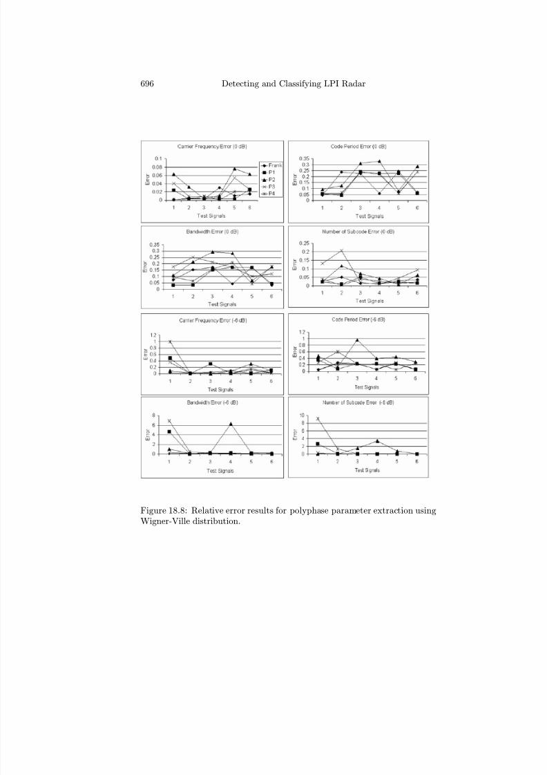
7/17/2019 1596932341 Intercept Radar.pdf
http://slidepdf.com/reader/full/1596932341-intercept-radarpdf 727/891
696 Detecting and Classifying LPI Radar
Figure 18.8: Relative error results for polyphase parameter extraction usingWigner-Ville distribution.
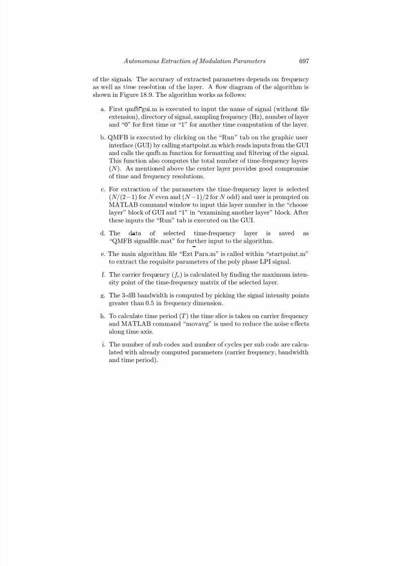
7/17/2019 1596932341 Intercept Radar.pdf
http://slidepdf.com/reader/full/1596932341-intercept-radarpdf 728/891
Autonomous Extraction of Modulation Parameters 697
of the signals. The accuracy of extracted parameters depends on frequencyas well as time resolution of the layer. A flow diagram of the algorithm isshown in Figure 18.9. The algorithm works as follows:
a. First qmfb gui.m is executed to input the name of signal (without fileextension), directory of signal, sampling frequency (Hz), number of layerand “0” for first time or “1” for another time computation of the layer.
b. QMFB is executed by clicking on the “Run” tab on the graphic userinterface (GUI) by calling startpoint.m which reads inputs from the GUIand calls the qmfb.m function for formatting and filtering of the signal.This function also computes the total number of time-frequency layers(N ). As mentioned above the center layer provides good compromiseof time and frequency resolutions.
c. For extraction of the parameters the time-frequency layer is selected
(N/(2−
1) for N even and (N −
1)/2 for N odd) and user is prompted onMATLAB command window to input this layer number in the “chooselayer” block of GUI and “1” in “examining another layer” block. Afterthese inputs the “Run” tab is executed on the GUI.
d. The data of selected time-frequency layer is saved as“QMFB signalfile.mat” for further input to the algorithm.
e. The main algorithm file “Ext Para.m” is called within “startpoint.m”to extract the requisite parameters of the poly phase LPI signal.
f. The carrier frequency (f c) is calculated by finding the maximum inten-sity point of the time-frequency matrix of the selected layer.
g. The 3-dB bandwidth is computed by picking the signal intensity pointsgreater than 0.5 in frequency dimension.
h. To calculate time period (T ) the time slice is taken on carrier frequencyand MATLAB command “movavg” is used to reduce the noise eff ectsalong time axis.
i. The number of sub codes and number of cycles per sub code are calcu-lated with already computed parameters (carrier frequency, bandwidthand time period).

7/17/2019 1596932341 Intercept Radar.pdf
http://slidepdf.com/reader/full/1596932341-intercept-radarpdf 729/891
698 Detecting and Classifying LPI Radar
Figure 18.9: Block diagram of QMFB parameter extraction algorithm.

7/17/2019 1596932341 Intercept Radar.pdf
http://slidepdf.com/reader/full/1596932341-intercept-radarpdf 730/891
Autonomous Extraction of Modulation Parameters 699
18.3.2 Testing the Algorithm
The information contained in the time-frequency QMFB layers can be used
to extract the parameters with reasonable accuracy using the algorithm de-scribed in this section. The middle time-frequency layer that is computedprovides a good compromise of time and frequency resolutions. for furtheranalysis of LPI signals. For extracting the carrier frequency and bandwidth of the signal, the signal processing could be restructured to examine the higherlayers for more accurate results. Similarly, for time period measurement, theinitial layers can yield better results. These accurate results will be at thecost of more computations and processing time. The algorithm should betested with a number of polyphase signals including Frank, P1, P2, P3, andP4 polyphase codes. We leave this an exercise for the student.
18.4 FMCW Parameters from Cyclostationary
Bifrequency Plane
This section demonstrates an algorithm to autonomously extract the mod-ulation parameters of a triangular FMCW signal using the spectral corre-lation density function. The signal processing uses the DFSM bifrequencyplane where the presence of the FMCW modulation has been identified. Theparameter extraction process determines the modulation period tm, modu-lation bandwidth ∆F and the carrier frequency f c. Extraction for low SNRbifrequency images gives reasonable results due to the denoising capability of the spectral correlation processing since noise is not correlated.
The DFSM algorithm first computes the spectral components of the signaland then executes the spectral correlation operations directly on the spectralcomponents. One important consideration in obtaining accurate results withthe FMCW extraction algorithm is to insure that the DFSM frequency res-olution, cycle frequency resolution selected, is small enough to measure theparameters accurately (for example, the code rate Rc).
As an example, an FMCW waveform with ∆F = 500 Hz, tm = 30 ms,f c = 1 kHz and SNR = 0 dB is processed through the DFSM algorithm.The frequency resolution was set to 16 Hz and the value of the Grenander’suncertainty condition is selected as M = 2 (N = 1,024). Due to the quadrantsymmetry of the bifrequency plane, the FMCW modulation shows up at fourdistinct locations as shown in Figure 18.10. Each of these four positionscontains a geometrical shape representative of the modulation from which allthe parameters can be extracted.
Two of the modulation parameters of interest are shown on the one se-
lected quadrant of the bifrequency plane shown in Figure 18.11. Both themodulation bandwidth and carrier frequency are easily recognized from thisresult. To extract the modulation period we closely examine the details re-
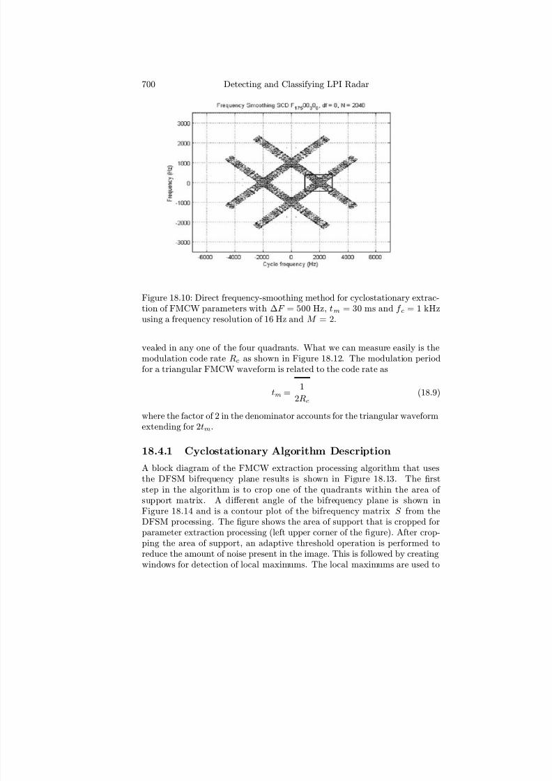
7/17/2019 1596932341 Intercept Radar.pdf
http://slidepdf.com/reader/full/1596932341-intercept-radarpdf 731/891
700 Detecting and Classifying LPI Radar
Figure 18.10: Direct frequency-smoothing method for cyclostationary extrac-tion of FMCW parameters with ∆F = 500 Hz, tm = 30 ms and f c = 1 kHzusing a frequency resolution of 16 Hz and M = 2.
vealed in any one of the four quadrants. What we can measure easily is themodulation code rate Rc as shown in Figure 18.12. The modulation periodfor a triangular FMCW waveform is related to the code rate as
tm = 1
2Rc
(18.9)
where the factor of 2 in the denominator accounts for the triangular waveformextending for 2tm.
18.4.1 Cyclostationary Algorithm Description
A block diagram of the FMCW extraction processing algorithm that usesthe DFSM bifrequency plane results is shown in Figure 18.13. The firststep in the algorithm is to crop one of the quadrants within the area of support matrix. A diff erent angle of the bifrequency plane is shown inFigure 18.14 and is a contour plot of the bifrequency matrix S from theDFSM processing. The figure shows the area of support that is cropped forparameter extraction processing (left upper corner of the figure). After crop-
ping the area of support, an adaptive threshold operation is performed toreduce the amount of noise present in the image. This is followed by creatingwindows for detection of local maximums. The local maximums are used to

7/17/2019 1596932341 Intercept Radar.pdf
http://slidepdf.com/reader/full/1596932341-intercept-radarpdf 732/891
Autonomous Extraction of Modulation Parameters 701
Figure 18.11: Bifrequency plane showing the measurement of FMCW modula-tion parameters ∆F = 500 Hz (frequency), and f c = 1 kHz (cycle frequency).
Figure 18.12: Bifrequency measurement of FMCW code rate on the cyclefrequency axis showing Rc = 16.6 Hz (=1/2tm).
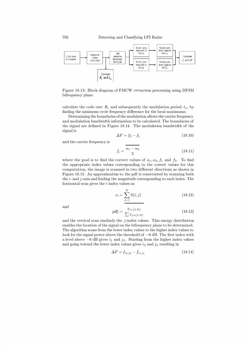
7/17/2019 1596932341 Intercept Radar.pdf
http://slidepdf.com/reader/full/1596932341-intercept-radarpdf 733/891
702 Detecting and Classifying LPI Radar
Figure 18.13: Block diagram of FMCW extraction processing using DFSMbifrequency plane.
calculate the code rate Rc and subsequently the modulation period tm byfinding the minimum cycle frequency diff erence for the local maximums.
Determining the boundaries of the modulation allows the carrier frequency
and modulation bandwidth information to be calculated. The boundaries of the signal are defined in Figure 18.14. The modulation bandwidth of thesignal is
∆F = f 2 − f 1 (18.10)
and the carrier frequency is
f c = α1 − α2
2 (18.11)
where the goal is to find the correct values of α1,α2, f 1 and f 2. To findthe appropriate index values corresponding to the correct values for thiscomputation, the image is scanned in two diff erent directions as shown inFigure 18.15. An approximation to the pdf is constructed by scanning boththe i- and j-axis and finding the magnitude corresponding to each index. Thehorizontal scan gives the i-index values as
xi =N j=1
S (i, j) (18.12)
and pdf i =
xi=(1:N )xj=(1:N )
(18.13)
and the vertical scan similarly the j-index values. This energy distributionenables the location of the signal on the bifrequency plane to be determined.The algorithm scans from the lower index values to the higher index values tolook for the signal power above the threshold of −6 dB. The first index witha level above −6 dB gives i
1 and j
1. Starting from the higher index values
and going toward the lower index values gives i2 and j2 resulting in
∆F = f i2,j2 − f i1,j1 (18.14)

7/17/2019 1596932341 Intercept Radar.pdf
http://slidepdf.com/reader/full/1596932341-intercept-radarpdf 734/891
Autonomous Extraction of Modulation Parameters 703
Figure 18.14: Contour plot of DFSM matrix S showing the region of supportbeing cropped for parameter extraction.
and
f c = αi1,j2 −
αi2,j1
2 (18.15)
The same algorithm is used to extract the parameters from a noisy signal.The scan method described above however, will smear the signal’s pdf so theprocedure for determining the index values must be modified to avoid possibleerrors (due to the high energy levels in the skirts of the pdf ). An adaptivenoise filter is also used here.
18.4.2 Testing the Algorithm
To evaluate the algorithm’s accuracy, the program is run for 12 diff erentsignals, which are listed below. The algorithm is also run for a set of higherfrequency signals. The program checks the signal for the existence of the
noise and uses the appropriate method to extract the parameters. The al-gorithm also checks the extracted parameters and does a closest match withthe possible threat signals in a database. This gives the exact parameters of

7/17/2019 1596932341 Intercept Radar.pdf
http://slidepdf.com/reader/full/1596932341-intercept-radarpdf 735/891
704 Detecting and Classifying LPI Radar
Figure 18.15: Scan geometry for DFSM matrix S to determine the correctindex values i and j .
the signal. The signals are analyzed using cyclo gui.m. The signals with nonoise and with 0 dB noise are analyzed with 16 Hz of frequency resolution butthe signals with −6 dB noise are analyzed with 32 Hz of frequency resolution.The high resolution selected for the −6 dB signals is due to the computationaldifficulties when using a personal computer. Hence the results for −6 dB sig-nals do not have a modulation period solution because the solutions are notreliable for the 32 Hz of resolution that is used. As discussed in Chapter 15,the resolution of the cycle frequency and frequency should be smaller thanthe largest parameter being measured or extracted.
F 1 7 250 20 s.mat (f c = 1 kHz, f s = 7 kHz, ∆F = 250 Hz, tm = 20 ms, signal only)F 1 7 250 30 s.mat (f c = 1 kHz, f s = 7 kHz, ∆F = 250 Hz, tm = 30 ms, signal only)F 1 7 500 20 s.mat (f c = 1 kHz, f s = 7 kHz, ∆F = 500 Hz, tm = 20 ms, signal only)F 1 7 500 30 s.mat (f c = 1 kHz, f s = 7 kHz, ∆F = 500 Hz, tm = 30 ms, signal only)
F 1 7 250 20 0.mat (f c = 1 kHz, f s = 7 kHz, ∆F = 250 Hz, tm = 20 ms, SNR = 0 dB)F 1 7 250 30 0.mat (f c = 1 kHz, f s = 7 kHz, ∆F = 250 Hz, tm = 30 ms, SNR = 0 dB)F 1 7 500 20 0.mat (f c = 1 kHz, f s = 7 kHz, ∆F = 500 Hz, tm = 20 ms, SNR = 0 dB)F 1 7 500 30 0.mat (f c = 1 kHz, f s = 7 kHz, ∆F = 500 Hz, tm = 30 ms, SNR = 0 dB)
F 1 7 250 20 -6.mat (f c = 1 kHz, f s = 7 kHz, ∆F = 250 Hz, tm = 20 ms, SNR = −6 dB)
F 1 7 250 30 -6.mat (f c = 1 kHz, f s = 7 kHz, ∆F = 250 Hz, tm = 30 ms, SNR = −
6 dB)F 1 7 500 20 -6.mat (f c = 1 kHz, f s = 7 kHz, ∆F = 500 Hz, tm = 20 ms, SNR = −6 dB)F 1 7 500 30 -6.mat (f c = 1 kHz, f s = 7 kHz, ∆F = 500 Hz, tm = 30 ms, SNR = −6 dB)

7/17/2019 1596932341 Intercept Radar.pdf
http://slidepdf.com/reader/full/1596932341-intercept-radarpdf 736/891
Autonomous Extraction of Modulation Parameters 705
18.5 Concluding Remarks
In this chapter, we have shown that we can extract the parameters for the
signal only measurements very accurately as shown in Figure 18.16. Theparameters extracted from the noisy signals are also fairly accurate, but thealgorithm for the noisy signals can be improved to get better performance.The threshold set for the noisy measurements were set to a fixed intuitivelevel, which is somewhat subjective. One may think of adding an adaptivethreshold that changes according to the noise level in the signal. Here we tookadvantage of the cyclostationary analysis to get rid of the noise. Note thatthe cyclostationary analysis has an inherited noise reducing process within itsspectral correlation algorithm. Once the signal is classified correctly, the exactparameters of the intercepted signal can be determined.
References
[1] Hejazi, M.R., Shevlyakov, G., and Ho, Y-S., “Modified discrete radontransforms and their application to rotation-invariant image analysis,”IEEE 8th Workshop on Multimedia Signal Processing , pp. 429—434,Oct. 2006.
[2] Minsheng, W., Chan, A.K., and Chui, C.K., “Linear frequency modu-lated signal detection using Radon-ambiguity transform,” IEEE Trans.
on Signal Processing , Vol. 26, No. 3, pp. 571—586, March 1998.
[3] Gulum, T. O., Pace, P. E. and Cristi, R. “Extraction of PolyphaseRadar Modulation Parameters Using a Wigner-Ville Distribution—RadonTransform,” IEEE International Conf. on Acoustics, Speech and SignalProcessing, Las Vegas, NV, March 2008.
[4] Gulum, T. O., “Autonomous Non-linear Classification of LPI RadarSignal Modulations,” Naval Postgraduate School Master’s Thesis, Sept.2007.
Problems
1. (QMFB) The files in the Part II folder Extract\POLY FROM QMFBperform the quadrature mirror filtering but have been modified to imple-ment the extraction routines in Section 18.3. (a) Generate a Frank codesignal with f c = 1 kHz, f s = 7 kHz, M = 16 and cpp = 2 for SNRs be-tween −10 dB and 10 dB (in steps of 1 dB). (b) Run poly from qmfb.mto extract the parameters for the Frank code. Be sure to follow the in-
structions on the command line that are displayed. (c) Plot the relativeerror as a function of the SNR for each of the extracted parameters. (d)Repeat (a)—(c) for the P4 code and compare your results.

7/17/2019 1596932341 Intercept Radar.pdf
http://slidepdf.com/reader/full/1596932341-intercept-radarpdf 737/891
706 Detecting and Classifying LPI Radar
Figure 18.16: Extraction results using the cyclostationary signal processingbifrequency plane.
7/17/2019 1596932341 Intercept Radar.pdf
http://slidepdf.com/reader/full/1596932341-intercept-radarpdf 738/891
Autonomous Extraction of Modulation Parameters 707
2. (QMFB) Edit the m-files contained in the Part II folderExtract\POLY FROM QMFB folder to analyze a diff erent layer (otherthan the middle layer). Repeat Problem 1 and compare your results.
3. (QMFB) Write a MATLAB procedure similar to Ext Para.m to extractthe parameters from an FMCW signal. Use the FMCW files in theTest Signals folder to evaluate your results.
4. (CYCLO) The files in the Part II folder Extract\FMCW FROM CYCLOperform the direct frequency smoothing spectral correlation techniqueto derive the bifrequency domain results. The file cyclo gui.m callsDFSM.m which has been modified to include the parameter extractionalgorithm described in Section 18.4. (a) Generate an FMCW signalwith f c = 1 kHz, f s = 7 kHz, ∆F = 500 Hz and tm = 30 ms for SNRsbetween −10 dB and 10 dB (in steps of 1 dB). (b) Run cyclo gui.m toextract the parameters of the FMCW waveforms. (c) Plot the relative
error as a function of the SNR for each of the extracted parameters. (d)Repeat (a)—(c) for an FMCW signal with twice the modulation band-width and compare your results.
5. (CYCLO) Copy the FAM.m file contained in the Part II folder CYCLOto the Extract\FMCW FROM CYCLO folder. Edit the file to includethe parameter extraction algorithm (see Problem 4). Repeat Problem4 (a)—(c) and compare your results.
6. (PWVD) The files in the Part II folder Extract\POLY FROM WVDperform the extraction of the polyphase parameters using the PWVD—Radon transform described in Section 18.2.1. The main filepoly from WVD.m uses a routine that cycles through the subfolder
“polyfi
les” to extract the parameters for all of the fi
les contained inthe folder. (a) Copy one example of each polyphase modulation forsignal only from the TestSignals folder (Part I) to the polyfiles folder.Edit the main file and change the diary file to represent your case un-der study. Run the parameter extraction algorithm and then computethe relative error for each result. (b) Repeat (a) for a SNR = 0 dB.(c) Repeat (a) for a SNR = −6 dB. (d) How does the noise aff ect therelative error for the extraction results?

7/17/2019 1596932341 Intercept Radar.pdf
http://slidepdf.com/reader/full/1596932341-intercept-radarpdf 739/891

7/17/2019 1596932341 Intercept Radar.pdf
http://slidepdf.com/reader/full/1596932341-intercept-radarpdf 740/891
Appendix A
Low Probability of
Intercept Toolbox
A.1 Introduction to the LPIT
The low probability of intercept toolbox is a collection of MATLAB files thatgive the user the quick capability to generate a number of LPI complex signalseasily. The user can change the parameters of the signal, plot out the signal’stime domain and power spectral density characteristics, and save the timedomain signal to the current directory for further analysis, using the time-frequency and bifrequency classification programs discussed in Part II.
The LPIT software is contained on the CD provided with this book, inthe folder titled LPIT. To install the toolbox, simply copy this folder to yourcomputer. When the LPI signals are generated, they are saved to the same
folder where the program files reside. After folder has been copied to yourcomputer, the following steps should then be followed to generate the signals:
1. Start MATLAB and change the current directory to the LPIT folder.
2. Type lpit on the command line to start the toolbox.
3. Choose one of the LPI signals on the menu and enter the parametersrequested.
4. Choose whether (or not) to plot the signal.
5. Choose whether (or not) to save the signals to the current directory.
Note that if the user chooses to save the signal, two .mat files are created:
one for the signal only, and one for the signal-plus-noise for SNR = 0 dB.
709
7/17/2019 1596932341 Intercept Radar.pdf
http://slidepdf.com/reader/full/1596932341-intercept-radarpdf 741/891
710 Detecting and Classifying LPI Radar
SNRs other than 0 dB can also be generated when supplying the requestedparameters. For each file, the complex signal is saved in a .mat file, withthe I and Q variables in two separate column vectors. The number of codeperiods generated by the LPIT is five (four for FMCW) although that caneasily be changed.
The 14 signal types available from the LPIT, and the corresponding chap-ter where they are discussed are shown below:1
1. FMCW (Chapter 4);
2. BPSK (Chapter 5);
3. Polyphase Barker codes (Chapter 5);
4. Polyphase Frank code (Chapter 5);
5. Polyphase code P1 (Chapter 5);
6. Polyphase code P2 (Chapter 5);
7. Polyphase code P3 (Chapter 5);
8. Polyphase code P4 (Chapter 5);
9. Polytime signals (Chapter 5).
10. Costas frequency hopping code (Chapter 6);
11. FSK/PSK (Costas) (Chapter 6);
12. FSK/PSK (Target) (Chapter 6);
13. Noise waveforms (Chapter 7);
14. Test signals (Chapters 9, 10, and 11);
A.2 Naming Convention and Example
For all signals, the name is automatically assigned to the .mat file, and reflectsthe signal parameters that were supplied by the user. The naming conven-tion is the same for each signal, but varies slighty due to diff erent parametersrequired for diff erent types of signals. The first character in the file name
1Taboada, F. L., “Detection and classification of low probability of intercept radar
signals using parallel filter arrays and higher order statistics,” Naval Postgraduate School,
Master’s Thesis, Sept. 2002.

7/17/2019 1596932341 Intercept Radar.pdf
http://slidepdf.com/reader/full/1596932341-intercept-radarpdf 742/891
Appendix A: Low Probability of Intercept Toolbox 711
Figure A.1: LPIT file naming convention.
always indicates the type of signal. The second character indicates the car-rier frequency (in kHz). The third character indicates the selected samplingfrequency (in kHz). The remaining characters are diff erent, depending on thetype of signal generated. The file naming convention is summarized in thetree diagram shown in Figure A.1
For example, for an FMCW, the fourth character is the modulation band-width (in Hz), and the fifth character is the modulation period (in ms). The
sixth character is either an “s” indicating signal only, or a number indicatingthe SNR for a noisy signal. Consider the signals F 1 7 250 20 s.mat (signalonly) and F 1 7 250 20 0.mat (SNR=0 dB). Here the F indicates FMCW.The 1 indicates an f c = 1 kHz carrier frequency, the 7 indicates f s = 7 kHzsampling frequency, the 250 indicates the modulation bandwidth ∆F = 250Hz, and the 20 represents the modulation period tm = 20× 10−3 s. The “s”in the first file name indicates that the .mat file contains only the signal. The“0” in the second file name indicates the .mat file with SNR = 0 dB. Forexample, if the signal is generated with a −6 dB SNR, then this value wouldbe 6. When the signals are saved, the names are always displayed, so theparameters chosen can be recognized.

7/17/2019 1596932341 Intercept Radar.pdf
http://slidepdf.com/reader/full/1596932341-intercept-radarpdf 743/891

7/17/2019 1596932341 Intercept Radar.pdf
http://slidepdf.com/reader/full/1596932341-intercept-radarpdf 744/891
Appendix B
Generating PAF Plots
Using the LPIT Files
For CW signals, the Web site by Levanon (www.eng.tau.ac.il/nadav/) in-cludes the files to calculate and display the autocorrelation function, the pe-riodic autocorrelation function, and the periodic ambiguity function.1 Thesefiles can be downloaded and used easily with the time domain signals gener-ated by the LPIT.
To calculate and display the ACF, PACF, and PAF, download the filesinto the LPIT folder. After generating the .mat files containing the LPI signal(see Appendix A), follow the steps below:
1. Run ambfn7.m (Levanon’s PAF code from the Web site).
2. Select “User Defined” in the first block at the top.
3. Deselect the Frequency Radio button that follows.
4. Next go to the command line and run the paf preprocess.m file distrib-uted with the LPIT. This file will ask the user to supply:
• Name of the signal file (.mat file that resides in the LPIT direc-tory);
• Sampling frequency f s (in Hz);
• Carrier frequency f c (in Hz);
1The MATLAB code to calculate the ambiguity function is described in Mozeson, E.,
and Levanon, N., “MATLAB code for plotting ambiguity functions,” IEEE Trans. on
Aerospace and Electronic Systems, Vol. 38, No. 3, 1064—1068, 2002.
713

7/17/2019 1596932341 Intercept Radar.pdf
http://slidepdf.com/reader/full/1596932341-intercept-radarpdf 745/891
714 Detecting and Classifying LPI Radar
• Number of code periods to include in PAF calculation N (1) forPSK and (2) for FSK.
5. Return to the ambfn7.m graphical user interface (GUI) and, next tothe sliders, enter in the five suggested values for the signal analysis.
6. On the GUI select Cal & Signal Plot first, then ACF and SPEC plot orPAF.
Note that the number of code periods N to include in ACF, PAF calculationis independent of the number of periods generated using the LPIT.

7/17/2019 1596932341 Intercept Radar.pdf
http://slidepdf.com/reader/full/1596932341-intercept-radarpdf 746/891
Appendix C
Primitive Roots and
Costas Sequences
In this appendix, a concise description of prime numbers, residues, reducedresidues, the Euler function φ(n), and primitive roots is given. The signifi-cance of this appendix is to present the concepts in a framework that lendsitself to the derivation of Costas frequency-hopping sequences. These con-cepts are useful for understanding the construction of Costas sequences usingthe Welch method .1
C.1 Primes
To begin we give the definition of a prime number.
Definition 1
An integer p > 1 is called a prime number, or a prime, in casethere is no divisor d of p satisfying 1 < d < p.
For example, the numbers 2, 3, 5, and 7 are prime numbers and there isan infinite number of primes. Although the numbers 4, 5, and 7 are not allprimes, they are all relatively prime with respect to each other, in that nonehave a common factor.2
1Note that mathematical concepts such as the division algorithm, the Euclidean algo-rithm for finding the greatest common divisor (gcd), and the solutions of simultaneouscongruencies using the Chinese remainder theorem are not described here, but a completetreatment is presented in Pace, P. E., Advanced Techniques for Digital Receivers, ArtechHouse, Inc., Norwood MA, 2000.
2
Niven, I., Zuckerman, H. S., and Montgomery, H. L., Introduction to the Theory of Numbers, 5th Edition , John Wiley and Sons, New York, 1991.
715
7/17/2019 1596932341 Intercept Radar.pdf
http://slidepdf.com/reader/full/1596932341-intercept-radarpdf 747/891
716 Detecting and Classifying LPI Radar
C.2 Complete and Reduced Residue Systems
If a congruence involves only addition, subtraction, and multiplication, we
may replace the integers with congruent integers. To help in this, the follow-ing definitions describing residue systems are given, followed by an exampleto illustrate the concept.
Definition 2
If h and j are two integers and h ≡ j(mod m), then we say that j is a residue of h modulo m.
Definition 3
The set of integers r1, r2, . . . , rs is called a complete residuesystem modulo m if ri = rj(mod m) and for each integer n therecorresponds an ri such that n ≡ ri(mod m).
If s diff erent integers r1, r2, . . . , rs form a complete residue system modulo m,then s = m. If m is a positive integer, then 0, 1, . . . , m − 1 is a completeresidue system modulo m. For example, for m = 7, the smallest positiveinteger values within the modulus are 0, 1, 2, 3, 4, 5, 6.
Definition 4
The set of integers r1, r2, . . . , rs is called a reduced residue sys-tem modulo m if (a) the gcd(ri, m) = 1 for each i, (b) ri =rj(mod m) whenever i = j , and (c) for each integer n relativelyprime to m there corresponds an ri such that n ≡ ri(mod m).
For example, the set 0, 1, 2, 3, 4, 5 is a complete residue system modulo 6,but 1, 5 is a reduced residue system modulo 6. That is, we can obtain areduced residue system from a complete residue system by simply deletingthose elements of the complete residue system that are not relatively primeto m.
Example 1 The sets 1, 2, 3, 0, 1, 2, −1, 0, 1, and 1, 5, 9 are all com-plete residue systems modulo 3.
When working with congruences modulo m, we can replace the integers inthe congruences by elements of 0, 1, 2, . . . , m − 1. This can make manycomplicated problems much easier.3
3Andrews, G. E., Number Theory, Dover Publications Inc., New York, 1971.

7/17/2019 1596932341 Intercept Radar.pdf
http://slidepdf.com/reader/full/1596932341-intercept-radarpdf 748/891
Appendix C: Primitive Roots and Costas Sequences 717
Example 2 Find an integer n that satisfies the congruence
325n ≡ 11(mod 3) (C.1)
Since325 ≡ 1(mod 3) (C.2)
and11 ≡ 2(mod 3) (C.3)
the problem is reduced to finding an integer n such that [15]
n ≡ 2(mod 3) (C.4)
The obvious answer here is the integer 2.
Definition 5
The function φ(m) denotes the number of positive integers less
than or equal to m that are relatively prime to m. This functionφ(m) is called the Euler φ−function, and represents the numberof integers that form the reduced residue system modulo m.
Example 3 We know φ(6) = 2 and 1, 5 is a reduced residue system modulo6. Note the set 5, 52 is also a reduced residue system modulo 6, since5 ≡ 5(mod 6) and 25 ≡ 1(mod 6).
C.3 Primitive Roots
We have examined the concept of the reduced residue system modulo p where p is a prime number. In this section, we present an integer g such thatg, g2, . . . , gφ( p) constitutes a reduced residue system modulo p. The integer
g is called a primitive root . Primitive roots are fundamental to how Costasfrequency sequences can be formed. An algorithm for deriving these types of sequences is presented, along with an example illustrating the method.
A few properties of reduced residue systems must now be given. The firstis that if h is the smallest positive integer such that
ah ≡ 1(mod m) (C.5)
we say that the order of a is h modulo m. If g is an integer, and the orderof g is φ(m) modulo m, then g is called a primitive root modulo m. Further,if g is a primitive root modulo m, then g, g2, . . . , gφ(m) makes up a reducedresidue system modulo m (sometimes referred to as a cyclic group).
Since the goal of this development is to derive a Costas sequence, the firststep is to determine a prime number p, remembering that the number of fre-
quencies in the FH sequence will be N F = p − 1. Also, since p is prime, wehave the following definition:

7/17/2019 1596932341 Intercept Radar.pdf
http://slidepdf.com/reader/full/1596932341-intercept-radarpdf 749/891
718 Detecting and Classifying LPI Radar
Definition 6
If p is prime, then there exist φφ p = φ p−1, primitive roots
modulo p.
This number can be determined by first eliminating those elements in thereduced residue set that are not relatively prime to p − 1, and then countingthe remaining entries. Note also that the order of a in (C.5) must be a divisorof φ( p) = p − 1.
Example 4 Consider the case for which p = 11, a prime number. Thenumber of frequencies in the Costas array will be N = p − 1 = 10. Thecomplete residue set is
0, 1, 2, 3, 4, 5, 6, 7, 8, 9, 10
There are p − 1 = 10 elements in the reduced residue set modulus 11
1, 2, 3, 4, 5, 6, 7, 8, 9, 10
and there are φ p − 1 = φ10 = 4 primitive roots. The questions we havenow are what are the primitive roots and what are the corresponding Costassequences?
To determine the primitive roots by which we can derive the Costas se-quences, we start with g = 1 (the first element in the reduced residue set).For g = 1 we have
11, 12, 13, . . . , 1φ11 = 1
and we say the order of 1 is 1. Consequently, 1 is not a primitive root. For 2,
21
, 22
, 23
, . . . , 2φ11
or
2, 4, 8, 5, 10, 9, 7, 3, 6, 1
and the order of 2 is 10, indicating that g = 2 is a primitive root. For 3 wehave,
3, 9, 5, 4, 1
and the order of 3 is 5. That is, 3 is not a primitive root. Continuing on forthe rest of the integers within the reduced residue system for 4 we have,
4, 5, 9, 3, 1
and the order of 4 is 5 (not a primitive root). For 5 we have,
5, 3, 4, 9, 1

7/17/2019 1596932341 Intercept Radar.pdf
http://slidepdf.com/reader/full/1596932341-intercept-radarpdf 750/891
Appendix C: Primitive Roots and Costas Sequences 719
and the order of 5 is 5 (not a primitive root). For 6 we have,
6, 3, 7, 9, 10, 5, 8, 4, 2, 1
so the order of 6 is 10, and consequently, 6 is a primitive root. For 7 we have,
7, 5, 2, 3, 10, 4, 6, 9, 8, 1
so the order of 7 is 10, and 7 is also a primitive root. For 8 we have,
8, 9, 6, 4, 10, 3, 2, 5, 7, 1
so the order of 8 is 10, and therefore 8 is a primitive root. Since we now haveour four primitive roots, we know that there are no more. For completenesshowever, we verify that for 9 we have,
9, 4, 3, 5, 1
and the order of 9 is 5 (not a primitive root), and for 10 we have,
10, 1
therefore the order of 10 is 2, and 10 is not a primitive root. In summary, thefour primitive roots are 2, 6, 7, 8.
One question still remains. How do we know, short of multiplying out, if ain (C.5) is a primitive root? That is, is there a way to find the primitive rootsand Costas sequences without having to calculate the order of each integervalue within the reduced residue set modulo p? Fortunately, the answer isyes, and we can use the following definition
Definition 7
If a is a primitive root modulus p then ar is a primitive rootmodulus p if and only if gcd(r, φ( p))=1 (r is relatively prime toφ( p) = p − 1).
In this case we can reduce our work by starting with the smallest value (e.g.,a = 2), and first determining if this is a primitive root. Once the smallestprimitive root is found, the others may be found easily by using the definitionabove.
In our example, since we have confirmed that a = 2 is a primitive root, weknow from the above definition that 2r is a primitive root modulus 11, if andonly if gcd(r,10)=1. So for r = 1, 21 = 2, for r = 3, 23 = 8, for r = 7, 27 = 7,and for r = 9, 29 = 6. In summary, the primitive roots are 2, 6, 7, 8 and thecorresponding sequences are Costas arrays. Also note that the Costas arrays
for a = 2 and a = 6 are reverse ordered (except for the 1 on the end). This isalso true for a = 7 and a = 8. This symmetry can be used to further simplifythe sequence calculations.

7/17/2019 1596932341 Intercept Radar.pdf
http://slidepdf.com/reader/full/1596932341-intercept-radarpdf 751/891

7/17/2019 1596932341 Intercept Radar.pdf
http://slidepdf.com/reader/full/1596932341-intercept-radarpdf 752/891
Appendix D
LPIsimNet
LPIsimNet is a collection of MATLAB files that let the user easily evaluate
the information network metrics and the SNR advantages of general nettedLPI radar topologies that were discussed in Chapter 10 including the presenceof an electronic attack or jammer. The objective of this tutorial is to have thestudent work several examples to become familiar with the program set. Theprogram set is organized as shown in Figure D.1. The “ScenarioEditor.m” filelets the student open a Graphical User Interface (GUI) and create a new “Sce-nario File” or modify an existing one. A “Result File” is generated after thestudent confirms the “Scenario File” and executes the simulation calculationwith the assistance of “Calculator.m.” The “SimulationViewer.m” is used toreview the “Result File” by examining the results grid. The “Painter.m” filesupports the drawing of the two GUI figures.
D.1 Overview of LPIsimNet ArchitectureThe LPIsimNet architecture can be used to set up a sensor network withany configuration and number of communication nodes. Evaluation of theinformation exchange capability and the operational tempo is presented tothe user using the sensor network metrics. LPI radar detection performanceand the SNR values of a network enabled configuration of emitters across anoperational landscape containing targets is also presented to the user includ-ing the ability to have the sensor nodes and jammer nodes move in time withany velocity.
721

7/17/2019 1596932341 Intercept Radar.pdf
http://slidepdf.com/reader/full/1596932341-intercept-radarpdf 753/891
722 Detecting and Classifying LPI Radar
Figure D.1: Program flow diagram.
D.1.1 Loading the Default Sensor Network
Start MATLAB and change the “Current Directory” to the folder where theLPIsimNet program resides. Run “ScenarioEditor.m” to open up the GUIbattlespace grid. You should see the grid as shown in Figure D.2. Theright side of the GUI is designed for displaying a schematic of the networktopology. Click the “Refresh Figure” to load the default network topology.The default network consists of N T = 3 nodes: NR1 (node-1); NR2 (node-2); and NR3 (node-3) which are capable both in information processing andsynchronized, coherent target detection. Note the links between these nodesare bidirectional. Click on the “Legend” and see the legend as shown in
Figure D.3. The legend describes the symbols on the grid and can be broughtup at any time.
D.1.2 Building a Scenario File and Running the
Simulation
Go back to the “ScenarioEditor.” In the top left corner is the “Top LevelProperties Panel” containing several generic simulation properties that mustbe set including the number of nodes, total time index(s) for including plat-form and target movement, decision tempo, deployment tempo, and the fight-ing tempo. The boundary of the X axis, and the boundary of the Y axis mustalso be set to model the battlespace landscape. For this tutorial, modify these
properties according to the values shown in Table D.1.

7/17/2019 1596932341 Intercept Radar.pdf
http://slidepdf.com/reader/full/1596932341-intercept-radarpdf 754/891
Appendix D: LPIsimNet 723
Figure D.2: ScenarioEditor battlespace grid.
Figure D.3: Symbol legend for LPIsimNet.

7/17/2019 1596932341 Intercept Radar.pdf
http://slidepdf.com/reader/full/1596932341-intercept-radarpdf 755/891
724 Detecting and Classifying LPI Radar
Table D.1: Top Level Properties For Scenario
Properties Values DescriptionNumber of nodes 3 Total number of nodes in networkTotal time indexes 1 Number of time steps in simulationDecision tempo 200 C2 decision tempoDeployment tempo 400 Tempo of deployment in OODAFighting tempo 300 Tempo of fighting in OODABoundary of X axis (km) 0, 100 Left, right battlespace boundaryBoundary of Y axis (km) 0, 100 Upper, lower battlespace boundary
The panel below the “Top Level Properties Panel” is the “Node PropertiesPanel.” The node properties panel contains the following scenario
information:
• Current node index;
• Type;
• Name;
• Initial position;
• Velocity;
• Availability of links to each node;
• Capability value K of information or jammer;
• Information rate λμ;
• Minimum information rate, λmin
μ ;
• ERP of radar or jammer;
• Eff ective antenna area Ae;
• Noise power.
The node properties for the Blue Force E2-C in the default simulation areshown in Figure D.4.

7/17/2019 1596932341 Intercept Radar.pdf
http://slidepdf.com/reader/full/1596932341-intercept-radarpdf 756/891
Appendix D: LPIsimNet 725
Figure D.4: Node properties.

7/17/2019 1596932341 Intercept Radar.pdf
http://slidepdf.com/reader/full/1596932341-intercept-radarpdf 757/891
726 Detecting and Classifying LPI Radar
Table D.2: Link Condition of 001
Node 1 Node 2 Node 3Availability of link N N Y
Table D.3: Parameters for Node 2 and Node 3
Properties Node2 Node3Type Blue Force Blue ForceName F-16 AC-130Initial position 20, 70 60, 70Velocity 0, 0 0, 0Links 101 110Cap. of info. or jamming 0.75 0.25Info. rate 200 300Min. info. rate 100 50ERP (W) 0 0Eff . antenna area 0 0Noise power 0 0
D.2 Setting the Node Properties
At the bottom of the “Node Properties Panel,” try switching between theproperties of the diff erent nodes. Note the “Node Index” that indicates thecurrent node. Set the properties of node 1 to the following values shown in
Figure D.4. The “Availability of Links to Each Node” represents the linkcondition to each node. For example, for node 1, 001 represents the linkconfiguration as shown in Table D.2. After setting node 1 availability, setnode 2 and node 3 to the values shown in Table D.3.
After setting all node properties needed, click “Refresh Figure” to see thelayout and the overall connection of this scenario. The topology should looklike that shown in Figure D.5.
Click “Save Scenario” and save the scenario file as “Sce-3C.mat.” Config-ure the MATLAB command line analysis to be visible along with the “Sce-narioEditor.” Click “Run Simulation” to activate the calculation of the sim-ulation results file. The MATLAB command line shows the tracking messageof the four phases in the calculation. Wait until a “Save As” dialog appearsand save the simulation results as “Sim-3C.mat.” Now, we have successfullyfinished creating a scenario file (Sce-3C.mat) and generated the simulationresults file (Sim-3C.mat).

7/17/2019 1596932341 Intercept Radar.pdf
http://slidepdf.com/reader/full/1596932341-intercept-radarpdf 758/891
Appendix D: LPIsimNet 727
Figure D.5: Simulation topology.

7/17/2019 1596932341 Intercept Radar.pdf
http://slidepdf.com/reader/full/1596932341-intercept-radarpdf 759/891
728 Detecting and Classifying LPI Radar
D.3 Viewing the Simulation Results
Go to the MATLAB environment and launch the “SimulationViewer.m.” The
SimulationViewer GUI grid appears as shown in Figure D.6. Click “Load” toload the simulation result file, “Sim-T1(3C).m” that was just generated. Afterloading, the simulation result file is displayed as shown in Figure D.7. Thevalues for the simulation properties are now shown in the top left “InformationNetwork Analysis Panel.” This panel consists of:
• Number of links suppressed;
• Reference Connectivity Measure;
• Connectivity Measure;
• Network Reach;
• Network Richness;
• Decision Tempo;
• Deployment Tempo;
• Fighting Tempo;
• Characteristic Tempo;
• Max Operational Tempo.
Observe the simulation results in the “Information Network Analysis Panel.”Click the “Detail” after the Reference Connectivity Measure. The detailedanalysis data is shown in the MATLAB command line as shown in Figure
D.8. Click the “Detail” after the Connectivity Measure. The detailed analy-sis data is shown in MATLAB command line as shown in Figure D.9. Clickthe “Detail” after the Reference Network Richness. The detailed analysisdata is shown in the MATLAB command line as shown in Figure D.10.
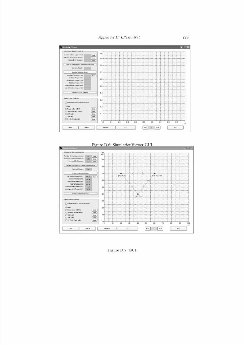
7/17/2019 1596932341 Intercept Radar.pdf
http://slidepdf.com/reader/full/1596932341-intercept-radarpdf 760/891
Appendix D: LPIsimNet 729
Figure D.6: SimulationViewer GUI.
Figure D.7: GUI.

7/17/2019 1596932341 Intercept Radar.pdf
http://slidepdf.com/reader/full/1596932341-intercept-radarpdf 761/891
730 Detecting and Classifying LPI Radar
Figure D.8: Reference connectivity measure C RM
for number of sensor networknodes N T = 3 to 20.
Figure D.9: Detailed results for connectivity measure.
Figure D.10: Detailed results for network richness.

7/17/2019 1596932341 Intercept Radar.pdf
http://slidepdf.com/reader/full/1596932341-intercept-radarpdf 762/891
Appendix D: LPIsimNet 731
Table D.4: LPI Radar Network: Scenario Setup for Three Nodes
Properties Node1 Node2 Node3 Node4Type Blue Force Blue Force Blue Hostile
Force JammerName E-2C F-16 AC-130 Su-34Initial position 40,40 20,70 60,70 80,40Velocity 0,0 0,0 0,0 -10,0Link configuration 0010 1010 1100 1000Cap. of info. or jamming 1.0 0.75 0.25 0.3Info. rate 200 200 300 0Min. info. rate 100 100 50 0ERP (W) 0 0 0 0Eff . antenna area (m2) 0 0 0 0Noise power (W) 0 0 0 0
D.4 Adding a Moving Jammer to the Scenario
Go back to the “ScenarioEditor.m” (if you have closed it, re-launch it) andload the scenario file Sim-3C.mat. In the “Top Level Properties Panel,”change the number of nodes to 4, and the total time index(s) to 3. Thatis, the scenario can evolve over time and the platforms within the scenariocan have movement. Each platform can also have a diff erent velocity (byincluding larger movements over a time index) in any general direction. Click“Refresh Figure” and see a fourth node, (NR4) node 4, that was added intothe network. Go to the “Node Properties Panel” and set the properties as in
Table D.4. Note the jammer is identified as being onboard an Su-34 “Flanker”fighter-bomber 2-seat strike aircraft. After refreshing, the figure should looklike Figure D.11.
Save this scenario as “Sce-3C+J.mat” and run the simulation calculationand save the result file as “Sim-3C+J.mat”. Go to “SimulationViewer” andload “Sim-3C+J.mat.” Your figure should look like Figure D.11. Note thetwo links to E-2C survive even with the Su-34 jammer. All the simulation re-sults in “Information Network Analysis” are identical to those of the previoussimulation. Click the double right arrows in the lower right section to switchthe time index to 2. Note that the Su-34 jammer moves closer to E-2C andthe link from AC-130 to E-2C is now not available (the arrow is missing). Atthis index the sensor information changes. The number of links suppressed innow one as shown in the “Information Network Analysis” panel. Click “De-tail” and review the detailed data in the MATLAB command line as shownin Figure D.12.
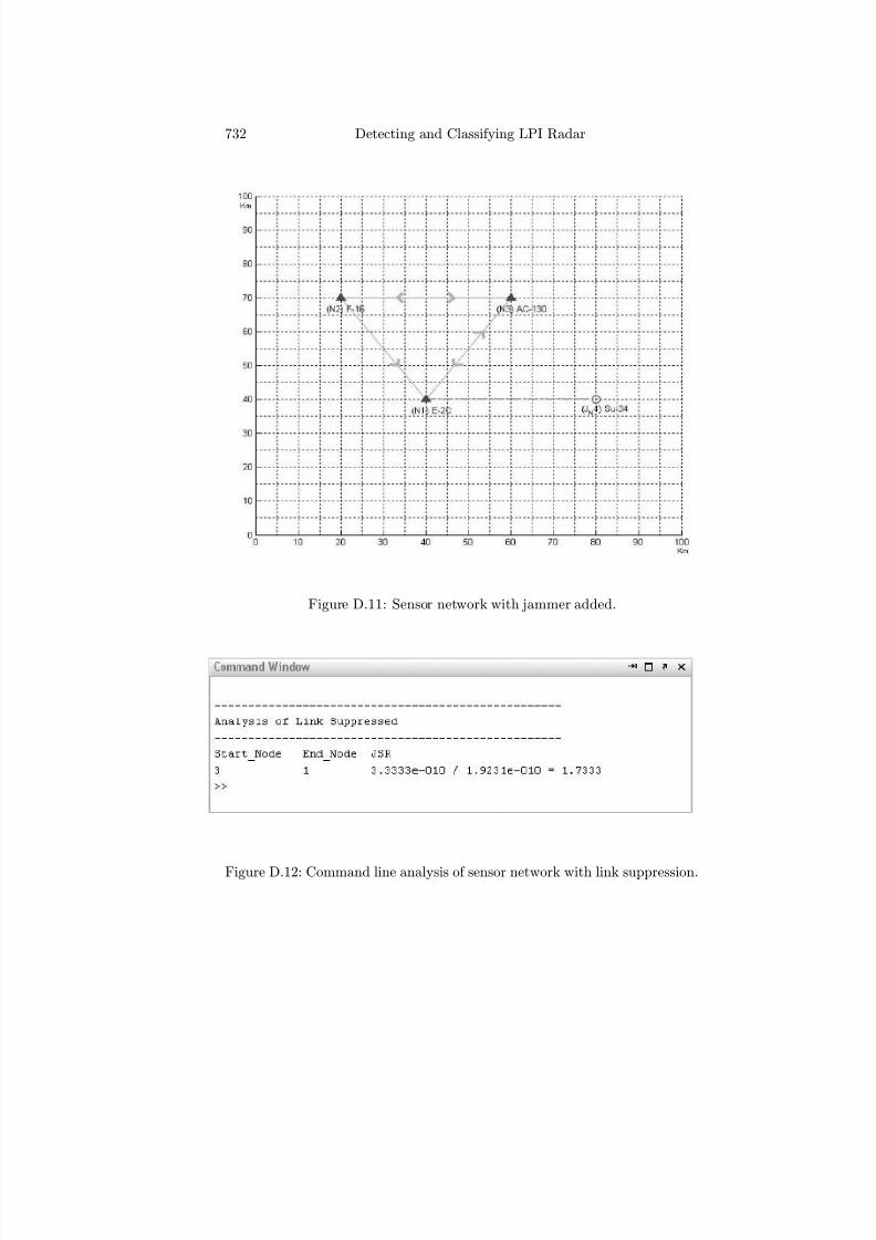
7/17/2019 1596932341 Intercept Radar.pdf
http://slidepdf.com/reader/full/1596932341-intercept-radarpdf 763/891
732 Detecting and Classifying LPI Radar
Figure D.11: Sensor network with jammer added.
Figure D.12: Command line analysis of sensor network with link suppression.

7/17/2019 1596932341 Intercept Radar.pdf
http://slidepdf.com/reader/full/1596932341-intercept-radarpdf 764/891
Appendix D: LPIsimNet 733
Table D.5: LPI Radar Network: Scenario Setup for the Three Nodes
Properties Node1 Node2 Node3 Node4Type Blue Force Blue Force Hostile Radar
Force Force Jammer TargetName Radar1 Radar2 Su-34 TargetInitial position 15,40 15,15 30,25 15,25Velocity 0,0 0,0 0,0 0,0Link configuration 0000 0000 1100 0000Cap. of info. or jamming 0 0 0 0Info. rate 0 0 0 0Min. info. rate 0 0 0 0ERP (W) 1000 100 10 0Eff . antenna area (m2) 0.0815 0.0815 0 0Noise power (W) 7.5 × 10⁻¹³ 1.0 × 10⁻¹² 0 0
Now click the double right arrows to increment the time index to 3. Notethat now two links are not available due to the new closer position of the
jammer. The “Trend” buttons provide the ability to review the trend of theresults as a function of time.
D.5 Netted Radar with a Jammer
To examine how a jammer influences a netted radar configuration, go to the“ScenarioEditor” and change the Number of nodes to 4, Number of Time
Indexes to 1. Set the node properties according to Table D.5. Click “RefreshFigure” to see Figure D.13.
Save this scenario as “Sce-2R+J+T.mat” and run the simulationcalculation. After the simulation completes save the result file as“Sim-2R+J+T.mat.” After saving the file go to “SimulationViewer” and load“Sim-2R+J+T.mat.” The figure should look like Figure D.14.
At the bottom left corner is the “Netted Radar Analysis Panel.” FigureD.15 describes several options that are applied to control the contour chartdisplay. Leave the “Enable Nework Synchronization” box unchecked andselect the “SNR(dB)” radial button. Click “Refresh” to see the SNR contourchart. It should look like Figure D.16. Note that this may take a few seconds.Click “Detail” for the SNR and the detailed analysis data is displayed in theMATLAB command line as shown in Figure D.17.
For a network-enabled configuration, check the “Enable Network Synchro-nization” in the “Netted Radar Analysis Panel” and click “Refresh” again.The SNR contour chart with the network synchronization should appear as

7/17/2019 1596932341 Intercept Radar.pdf
http://slidepdf.com/reader/full/1596932341-intercept-radarpdf 765/891
734 Detecting and Classifying LPI Radar
Figure D.13: Topology of simulation: two emitters, one target, one jammer.
Figure D.14: Radar network properties with jammer added.

7/17/2019 1596932341 Intercept Radar.pdf
http://slidepdf.com/reader/full/1596932341-intercept-radarpdf 766/891
Appendix D: LPIsimNet 735
Figure D.15: Description of netted radar analysis panel.
shown as Figure D.18. Click “Detail” for the SNR, and the detailed analysisdata is displayed in the MATLAB command line as shown in Figure D.19.
To examine the eff ects of the jammer, uncheck “Enable Network Simula-tion” and select the “S/N+J” Ratio (dB)” radial button. Then click “Re-fresh.” The eff ect of hostile jamming on the netted radar systems and sensornetwork can be examined by reviewing the SNJR contour chart as shown inFigure D.20. In this figure, the network connecting the radar sensors is dis-abled. Click the “Detail” of S/N+J and view the detailed analysis as displayedin Figure D.21. The contour chart and the detailed analysis show that with-out the network, the S/N+J = −70 dB at the target. If the sensor network isenabled however, the S/N+J increases as shown in the contours displayed inFigure D.22. The command line analysis shows the S/N+J = −64 dB when
the network is enabled.

7/17/2019 1596932341 Intercept Radar.pdf
http://slidepdf.com/reader/full/1596932341-intercept-radarpdf 767/891
736 Detecting and Classifying LPI Radar
Figure D.16: SNR contour chart without network synchronization.
Figure D.17: Command line analysis of SNR—no network.

7/17/2019 1596932341 Intercept Radar.pdf
http://slidepdf.com/reader/full/1596932341-intercept-radarpdf 768/891
Appendix D: LPIsimNet 737
Figure D.18: SNR contour chart with network synchronization.
Figure D.19: Command line analysis of SNR—with network.
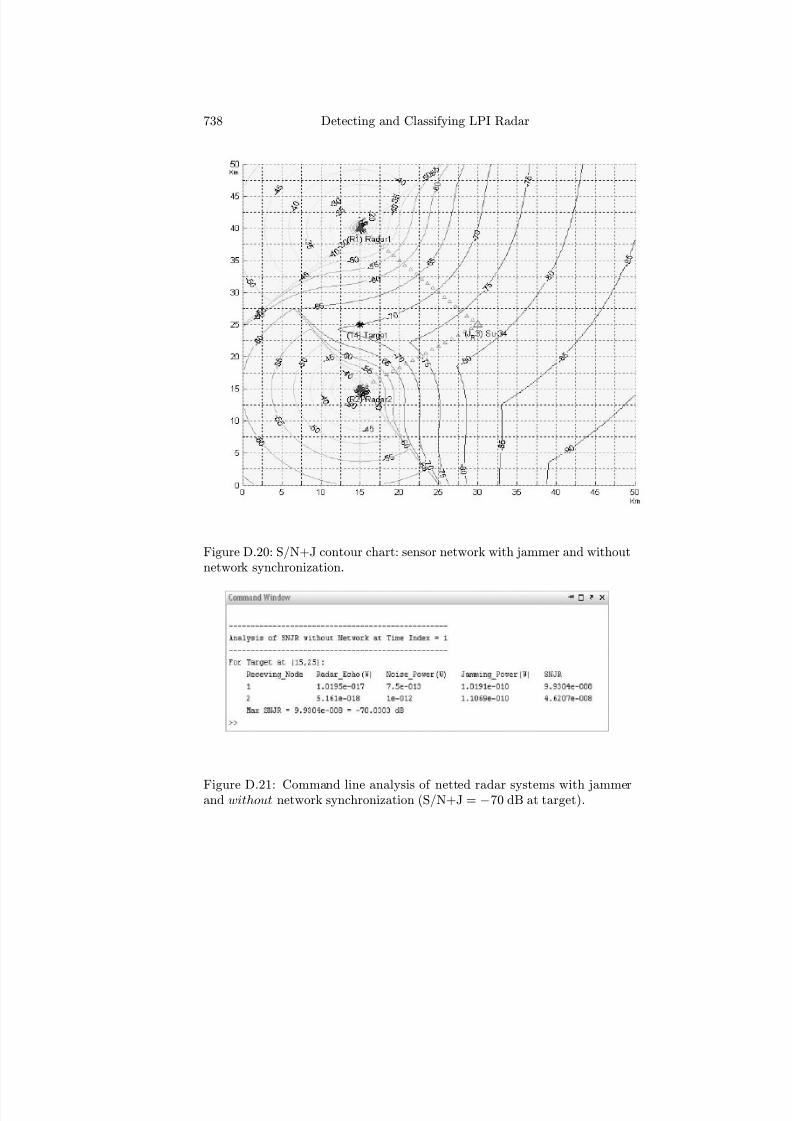
7/17/2019 1596932341 Intercept Radar.pdf
http://slidepdf.com/reader/full/1596932341-intercept-radarpdf 769/891
738 Detecting and Classifying LPI Radar
Figure D.20: S/N+J contour chart: sensor network with jammer and withoutnetwork synchronization.
Figure D.21: Command line analysis of netted radar systems with jammerand without network synchronization (S/N+J = −70 dB at target).

7/17/2019 1596932341 Intercept Radar.pdf
http://slidepdf.com/reader/full/1596932341-intercept-radarpdf 770/891
Appendix D: LPIsimNet 739
Figure D.22: S/N+J contour chart: netted radar systems with jammer andwith network synchronization.
Figure D.23: Command line analysis of sensor network with jammer andwithout network synchronization (S/N+J = −64 dB at target).

7/17/2019 1596932341 Intercept Radar.pdf
http://slidepdf.com/reader/full/1596932341-intercept-radarpdf 771/891

7/17/2019 1596932341 Intercept Radar.pdf
http://slidepdf.com/reader/full/1596932341-intercept-radarpdf 772/891
Appendix E
PWVD for FMCW with
∆F = 500 Hz
In Figures E.1 and E.2, a signal with f c = 1,000 Hz, tm = 20 ms and∆F = 500 Hz is examined using the PWVD. In Figure E.1(a) the increasein bandwidth is noticeable and in the time-frequency distribution in FigureE.1(b), the important parameters can all be extracted. In Figure E.2(a), theSNR = 0 dB, and the signal is still visible and the parameters can be ex-tracted. In Figure E.2(b) the increase in noise is apparent (SNR = −6 dB),but the parameters can still be extracted.
741

7/17/2019 1596932341 Intercept Radar.pdf
http://slidepdf.com/reader/full/1596932341-intercept-radarpdf 773/891
742 Detecting and Classifying LPI Radar
Figure E.1: PWVD for FMCW with ∆F = 500 Hz, tm = 30 ms (signal only),showing the (a) marginal frequency domain, and (b) time-frequency plot.

7/17/2019 1596932341 Intercept Radar.pdf
http://slidepdf.com/reader/full/1596932341-intercept-radarpdf 774/891
Appendix E: PWVD for FMCW with ∆F = 500 Hz 743
Figure E.2: PWVD for FMCW with ∆F = 500 Hz, tm = 30 ms, time-frequency plot for (a) SNR = 0 dB, and (b) SNR = −6 dB.

7/17/2019 1596932341 Intercept Radar.pdf
http://slidepdf.com/reader/full/1596932341-intercept-radarpdf 775/891

7/17/2019 1596932341 Intercept Radar.pdf
http://slidepdf.com/reader/full/1596932341-intercept-radarpdf 776/891
Appendix F
PWVD for Frank Code
with T = 64 ms
In the second example of a Frank signal using the PWVD, the signal has acarrier frequency of f c = 1,000 Hz, 64 phase codes (M = 8), and a cpp = 1.The signal has a code period of T = N 2tb = 64 ms. Figure F.1(a) shows thePWVD frequency domain plot. As expected, due to the longer code length(N c = M 2 = 64), the modulation spikes that were clearly visible in Figure9.16(a) (N c = M 2 = 16) are now hard to distinguish. Figure F.1(b) showsthe PWVD time-frequency plot, and indicates the bandwidth measurementand code period measurement. Figure F.2(a) shows the time-frequency plotwith SNR = 0 dB. All parameters can still be extracted. In Figure F.2(b),however (SNR = −6 dB), identification of the major crossterm and themeasurements of the signal parameters become more difficult.
745
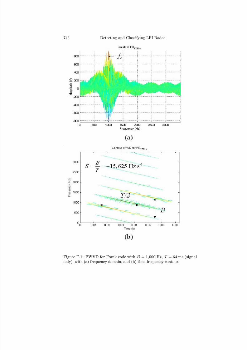
7/17/2019 1596932341 Intercept Radar.pdf
http://slidepdf.com/reader/full/1596932341-intercept-radarpdf 777/891
746 Detecting and Classifying LPI Radar
Figure F.1: PWVD for Frank code with B = 1,000 Hz, T = 64 ms (signalonly), with (a) frequency domain, and (b) time-frequency contour.
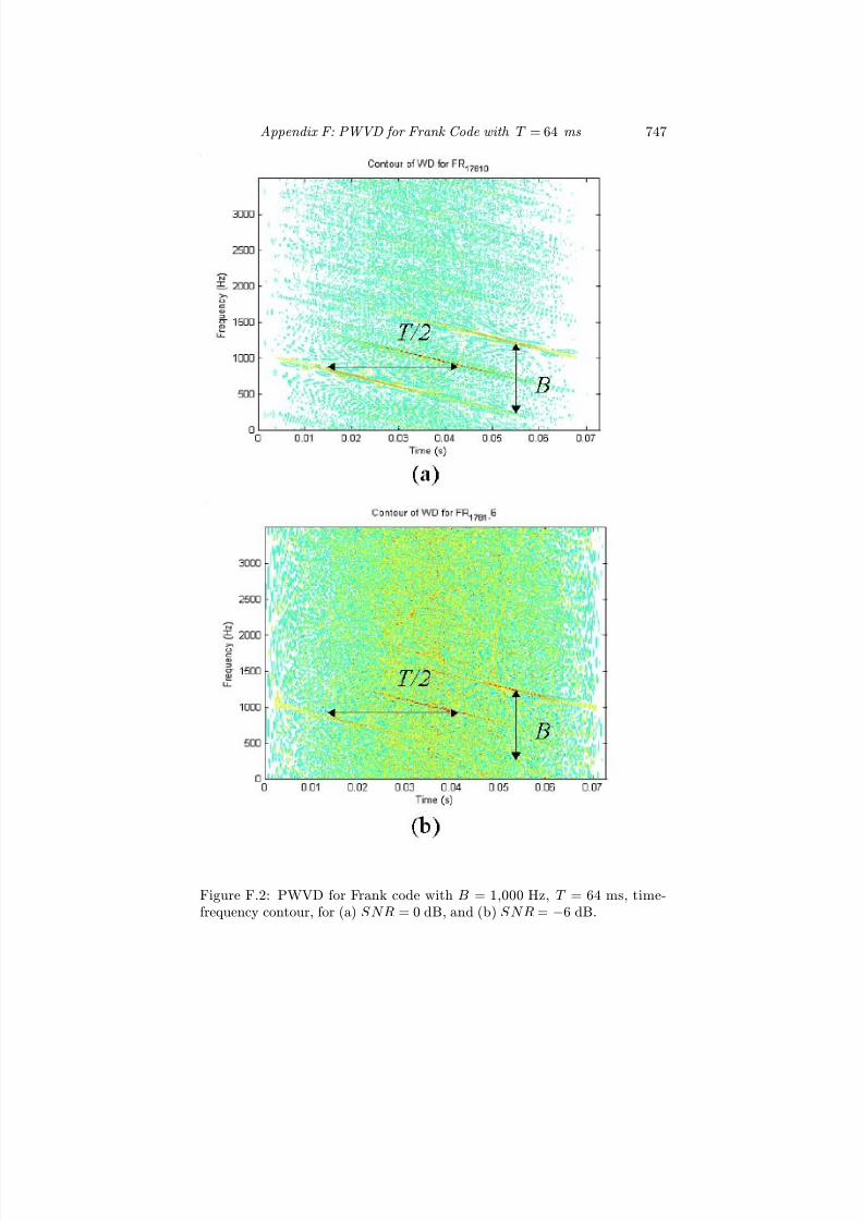
7/17/2019 1596932341 Intercept Radar.pdf
http://slidepdf.com/reader/full/1596932341-intercept-radarpdf 778/891
Appendix F: PWVD for Frank Code with T = 64 ms 747
Figure F.2: PWVD for Frank code with B = 1,000 Hz, T = 64 ms, time-frequency contour, for (a) SNR = 0 dB, and (b) SNR = −6 dB.

7/17/2019 1596932341 Intercept Radar.pdf
http://slidepdf.com/reader/full/1596932341-intercept-radarpdf 779/891

7/17/2019 1596932341 Intercept Radar.pdf
http://slidepdf.com/reader/full/1596932341-intercept-radarpdf 780/891
Appendix G
PWVD Results for P1, P2,
P3, and P4 Codes
G.1 P1 Code Analysis
In this section, the PWVD is used to extract the parameters from a P1 phase-coded CW signal. The intercepted signal shown in the following example hasa carrier frequency of f c = 1,000 Hz, a cpp = 1 (B = 1,000 Hz), 64 phasecodes (N c = 64), and is sampled by the ADC at a rate of f s = 7,000 Hz.
The marginal frequency domain result is shown in Figure G.1(a). Herethe harmonics are not as evident, without zooming in on the signal in thefrequency domain. Figure G.1(b) demonstrates the P1 modulation in thetime-frequency domain, and reveals that a longer code period makes it easierto identify the major crossterm in order to make the signal measurements.
Notice that the slopes of each line are negative. It is interesting to note thatif the crossterms were deleted, the parameter measurements might not beeasier to extract. Figure G.2(a) shows the SNR = 0 dB results. Extractionis still possible, but in Figure G.2(b) with SNR = −6 dB, this capabilityagain disappears quickly.
G.2 P2 Code Analysis
The P2 code shows up in the PWVD in a similar manner as the P1 andFrank code, except the slope is positive. Since the code period T = N 2c tbboth (12.27) and (12.28) apply. The signal examined has f c = 1,000 Hz,a cpp = 1 and 64 phase codes (N c = 64). Figure G.3(a) shows the phase-
coded signal with a code period of 64 ms. Note the eff ect the additional code
749
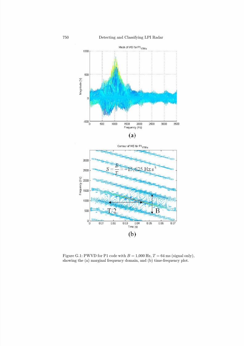
7/17/2019 1596932341 Intercept Radar.pdf
http://slidepdf.com/reader/full/1596932341-intercept-radarpdf 781/891
750 Detecting and Classifying LPI Radar
Figure G.1: PWVD for P1 code with B = 1,000 Hz, T = 64 ms (signal only),showing the (a) marginal frequency domain, and (b) time-frequency plot.

7/17/2019 1596932341 Intercept Radar.pdf
http://slidepdf.com/reader/full/1596932341-intercept-radarpdf 782/891
Appendix G: PWVD Results for P1, P2, P3, and P4 Codes 751
Figure G.2: PWVD for P1 code with B = 1,000 Hz, T = 64 ms, time-frequency plot, for (a) SNR = 0 dB, and (b) SNR = −6 dB.
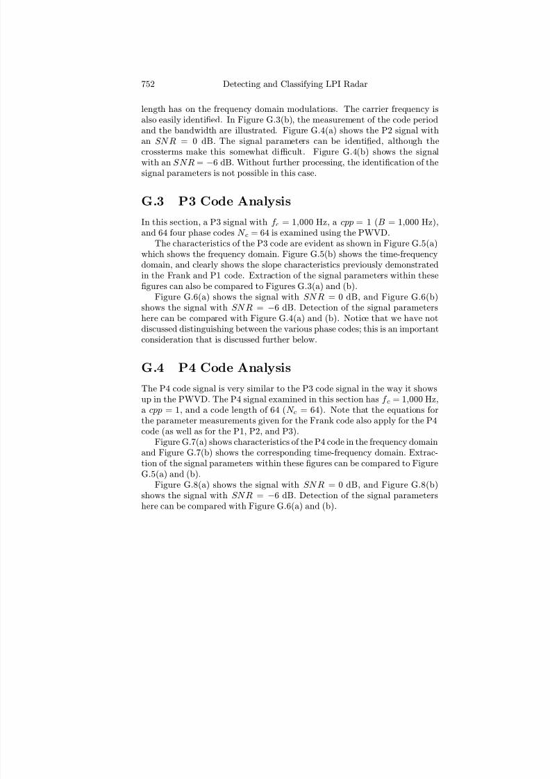
7/17/2019 1596932341 Intercept Radar.pdf
http://slidepdf.com/reader/full/1596932341-intercept-radarpdf 783/891
752 Detecting and Classifying LPI Radar
length has on the frequency domain modulations. The carrier frequency isalso easily identified. In Figure G.3(b), the measurement of the code periodand the bandwidth are illustrated. Figure G.4(a) shows the P2 signal withan SNR = 0 dB. The signal parameters can be identified, although thecrossterms make this somewhat difficult. Figure G.4(b) shows the signalwith an SNR = −6 dB. Without further processing, the identification of thesignal parameters is not possible in this case.
G.3 P3 Code Analysis
In this section, a P3 signal with f c = 1,000 Hz, a cpp = 1 (B = 1,000 Hz),and 64 four phase codes N c = 64 is examined using the PWVD.
The characteristics of the P3 code are evident as shown in Figure G.5(a)which shows the frequency domain. Figure G.5(b) shows the time-frequencydomain, and clearly shows the slope characteristics previously demonstrated
in the Frank and P1 code. Extraction of the signal parameters within thesefigures can also be compared to Figures G.3(a) and (b).
Figure G.6(a) shows the signal with SNR = 0 dB, and Figure G.6(b)shows the signal with SNR = −6 dB. Detection of the signal parametershere can be compared with Figure G.4(a) and (b). Notice that we have notdiscussed distinguishing between the various phase codes; this is an importantconsideration that is discussed further below.
G.4 P4 Code Analysis
The P4 code signal is very similar to the P3 code signal in the way it showsup in the PWVD. The P4 signal examined in this section has f c = 1,000 Hz,
a cpp = 1, and a code length of 64 (N c = 64). Note that the equations forthe parameter measurements given for the Frank code also apply for the P4code (as well as for the P1, P2, and P3).
Figure G.7(a) shows characteristics of the P4 code in the frequency domainand Figure G.7(b) shows the corresponding time-frequency domain. Extrac-tion of the signal parameters within these figures can be compared to FigureG.5(a) and (b).
Figure G.8(a) shows the signal with SNR = 0 dB, and Figure G.8(b)shows the signal with SNR = −6 dB. Detection of the signal parametershere can be compared with Figure G.6(a) and (b).

7/17/2019 1596932341 Intercept Radar.pdf
http://slidepdf.com/reader/full/1596932341-intercept-radarpdf 784/891
Appendix G: PWVD Results for P1, P2, P3, and P4 Codes 753
Figure G.3: PWVD for P2 code with B = 1,000 Hz, T = 64 ms (signal only),showing the (a) marginal frequency domain, and (b) time-frequency domain.

7/17/2019 1596932341 Intercept Radar.pdf
http://slidepdf.com/reader/full/1596932341-intercept-radarpdf 785/891
754 Detecting and Classifying LPI Radar
Figure G.4: PWVD for P2 code with B = 1,000 Hz, T = 64 ms, time-frequency plot, for (a) SNR = 0 dB, and (b) SNR = −6 dB.

7/17/2019 1596932341 Intercept Radar.pdf
http://slidepdf.com/reader/full/1596932341-intercept-radarpdf 786/891
Appendix G: PWVD Results for P1, P2, P3, and P4 Codes 755
Figure G.5: PWVD for P3 code with B = 1,000 Hz, T = 64 ms (signal only),showing the (a) marginal frequency domain, and (b) time-frequency plot.
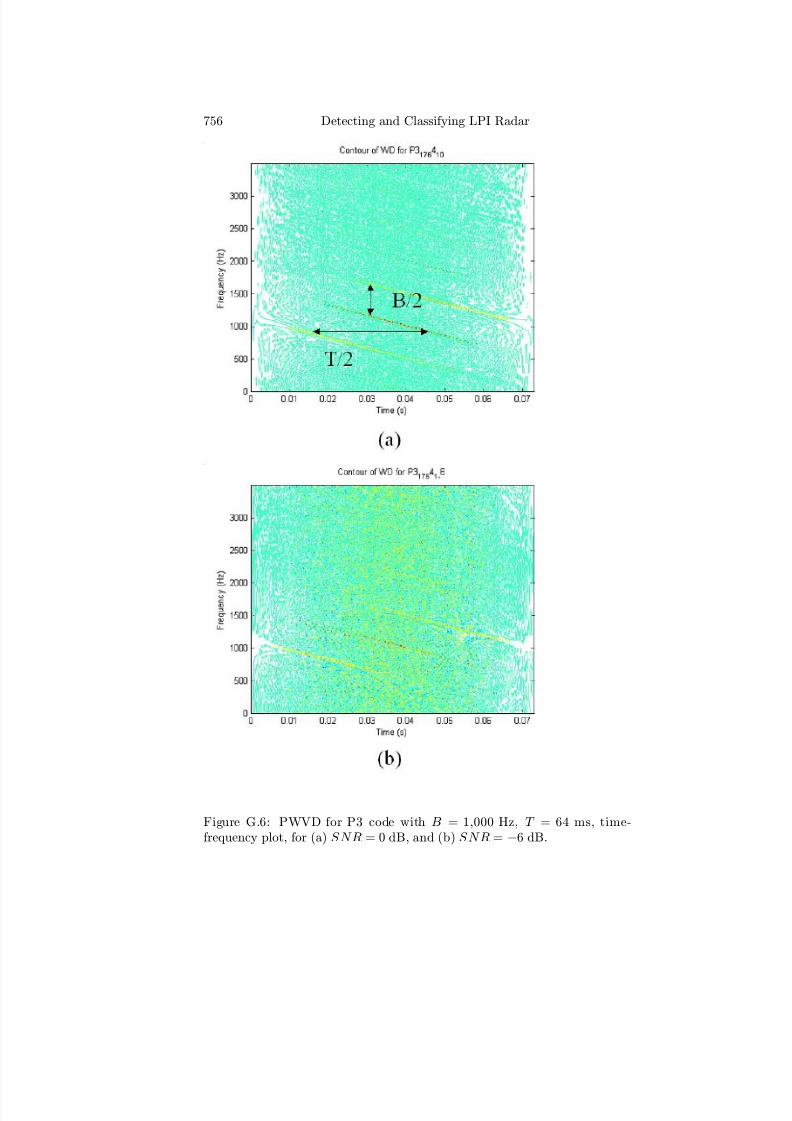
7/17/2019 1596932341 Intercept Radar.pdf
http://slidepdf.com/reader/full/1596932341-intercept-radarpdf 787/891
756 Detecting and Classifying LPI Radar
Figure G.6: PWVD for P3 code with B = 1,000 Hz, T = 64 ms, time-frequency plot, for (a) SNR = 0 dB, and (b) SNR = −6 dB.
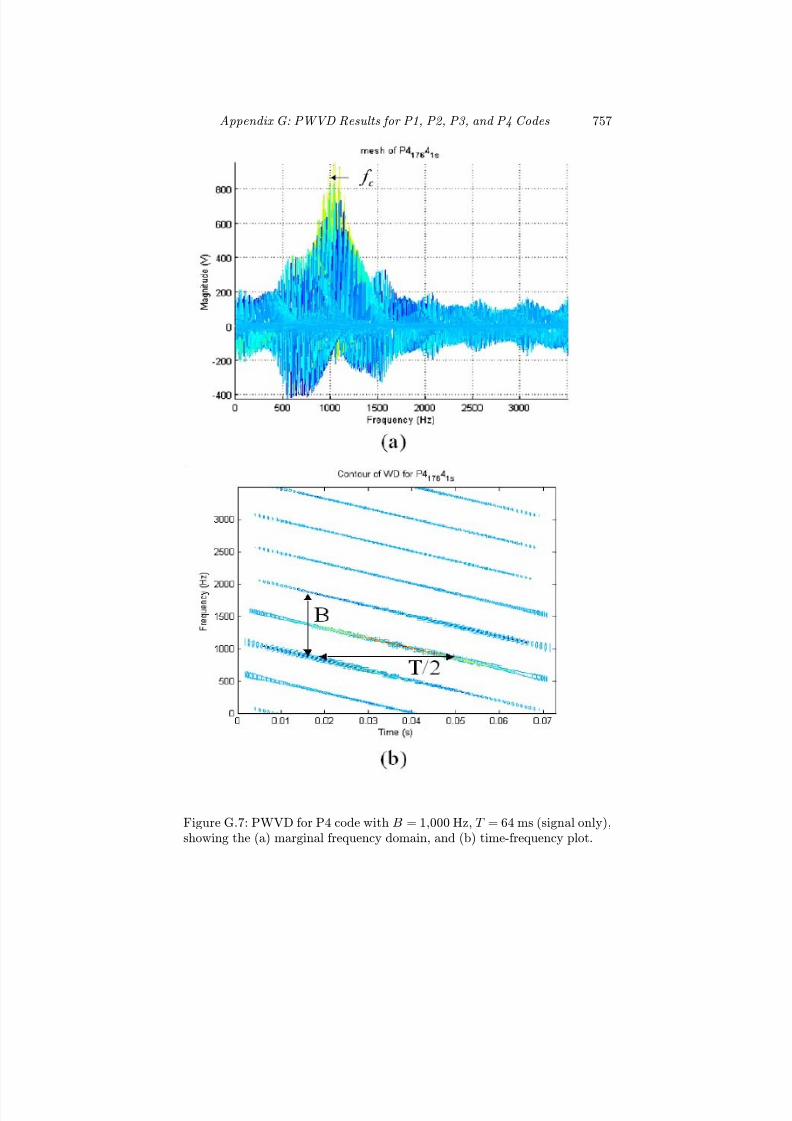
7/17/2019 1596932341 Intercept Radar.pdf
http://slidepdf.com/reader/full/1596932341-intercept-radarpdf 788/891
Appendix G: PWVD Results for P1, P2, P3, and P4 Codes 757
Figure G.7: PWVD for P4 code with B = 1,000 Hz, T = 64 ms (signal only),showing the (a) marginal frequency domain, and (b) time-frequency plot.

7/17/2019 1596932341 Intercept Radar.pdf
http://slidepdf.com/reader/full/1596932341-intercept-radarpdf 789/891
758 Detecting and Classifying LPI Radar
Figure G.8: PWVD for P4 code with B = 1,000 Hz, T = 64 ms, time-frequency plot, for (a) SNR = 0 dB, and (b) SNR = −6 dB.

7/17/2019 1596932341 Intercept Radar.pdf
http://slidepdf.com/reader/full/1596932341-intercept-radarpdf 790/891
Appendix H
PWVD Results forPolytime Codes T2, T3,
and T4
H.1 T2(2) Polytime Code
The T2(2) signal examined with the PWVD has the same parameters as theT1(2) signal investigated above, except that it has a zero beat at its carrierfrequency. Figure H.1(a) shows the PWVD frequency domain for the T2(2).The energy is not as evenly spread out as the T1(2) previously shown, and astrong negative component at the carrier frequency is evident. Figure H.1(b)shows the time-frequency distribution, and shows a unique pattern of X’s
centered about the carrier (due to the zero beat at the carrier frequency). Themeasurement of the bandwidth B and code period T are also shown, althoughthis is somewhat more difficult without any post-PWVD image processing.
To understand the bandwidth characteristics shown in Figure H.1, thephase shift for the T2(2) is shown in Figure H.2. Here, the shortest phasechange is eight samples long, or 1.143 ms. This results in a bandwidth ex-cursion of 875 Hz, as shown. Figure H.3(a) shows the signal for an SNR = 0dB. The signal can still be identified as a T2(2), but it is much more difficultto do compared to the T1(2). Errors can also occur when the parameters areextracted. In Figure H.3(b) with a SNR = −6 dB, no signal identificationcan be made, and no parameters can be extracted without any post-PWVDimage processing.
759

7/17/2019 1596932341 Intercept Radar.pdf
http://slidepdf.com/reader/full/1596932341-intercept-radarpdf 791/891
760 Detecting and Classifying LPI Radar
Figure H.1: PWVD for polytime code T2(2) with B = 875 Hz, T = 16ms (signal only), showing the (a) marginal frequency domain, and (b) time-frequency plot.
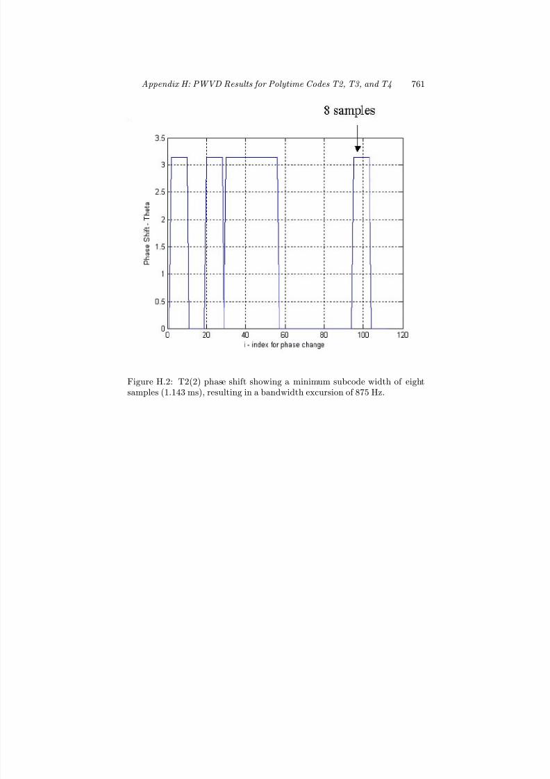
7/17/2019 1596932341 Intercept Radar.pdf
http://slidepdf.com/reader/full/1596932341-intercept-radarpdf 792/891
Appendix H: PWVD Results for Polytime Codes T2, T3, and T4 761
Figure H.2: T2(2) phase shift showing a minimum subcode width of eightsamples (1.143 ms), resulting in a bandwidth excursion of 875 Hz.

7/17/2019 1596932341 Intercept Radar.pdf
http://slidepdf.com/reader/full/1596932341-intercept-radarpdf 793/891
762 Detecting and Classifying LPI Radar
Figure H.3: PWVD for polytime code T2(2) code with B = 875 Hz, T = 16ms, showing the time-frequency plot, for (a) SNR = 0 dB, and (b) SNR = −6dB.

7/17/2019 1596932341 Intercept Radar.pdf
http://slidepdf.com/reader/full/1596932341-intercept-radarpdf 794/891
Appendix H: PWVD Results for Polytime Codes T2, T3, and T4 763
H.2 T3(2) Polytime Code
The T3(2) is examined next, and represents an approximation of a linearFM waveform with modulation bandwidth ∆F . As discussed in Chapter 5,the T3(2) is generated from the quadratic linear FM phase trajectory, witha zero beat at its beginning. Figure H.4(a) shows the PWVD frequencydomain for the signal-only case, with ∆F = 600 Hz and modulation periodtm = T = 16 ms. Figure H.4(b) shows the time-frequency image with themodulation bandwidth and modulation period indicated. Note the similarityto Figure 9.18(a) and (b).
To understand the bandwidth characteristics shown in Figure H.4, thephase shift for the T3(2) is shown in Figure H.5. With six samples makingup the shortest phase change (0.857 ms), the bandwidth excursion is 1,167Hz (approximately 2∆F ). The PWVD results for the T3(2) with SNR = 0and SNR = −6 dB are shown in Figure H.6(a) and (b), respectively.
H.3 T4(2) Polytime Code
The T4(2) code for a ∆F = 600 Hz and tm =16 ms is shown in Figure H.7To understand the bandwidth characteristics shown in Figure H.7, the phaseshift for the T4(2) is shown in Figure H.8. The smallest phase change hereis again six samples resulting in a bandwidth excursion of 1,167 Hz. FigureH.9 shows the PWVD for the T4(2) code with Figure H.9(a) showing theSNR = 0 dB case and Figure H.9(b) showing the SNR = −6 dB case (∆F =600 Hz, B = 1,167 Hz).

7/17/2019 1596932341 Intercept Radar.pdf
http://slidepdf.com/reader/full/1596932341-intercept-radarpdf 795/891
764 Detecting and Classifying LPI Radar
Figure H.4: PWVD for polytime code T3(2) with ∆F = 600 Hz, B = 1,167Hz, and tm = T = 16 ms (signal only), showing the (a) marginal frequencydomain and (b) time-frequency plot.

7/17/2019 1596932341 Intercept Radar.pdf
http://slidepdf.com/reader/full/1596932341-intercept-radarpdf 796/891
Appendix H: PWVD Results for Polytime Codes T2, T3, and T4 765
Figure H.5: T3(2) phase shift showing a minimum subcode width of six sam-ples (0.857 ms), resulting in a bandwidth excursion of 1,167 Hz.

7/17/2019 1596932341 Intercept Radar.pdf
http://slidepdf.com/reader/full/1596932341-intercept-radarpdf 797/891
766 Detecting and Classifying LPI Radar
Figure H.6: PWVD for T3(2) code with ∆F = 600 Hz, B = 1,167 Hz, andtm = T = 16 ms, showing the time-frequency plot for (a) SNR = 0 dB, and(b) SNR = −6 dB.

7/17/2019 1596932341 Intercept Radar.pdf
http://slidepdf.com/reader/full/1596932341-intercept-radarpdf 798/891
Appendix H: PWVD Results for Polytime Codes T2, T3, and T4 767
Figure H.7: PWVD for T4(2) code with ∆F = 600 Hz, B = 1,167 Hz,tm = T = 16 ms (signal only), showing the (a) marginal frequency domain,and (b) time-frequency plot.
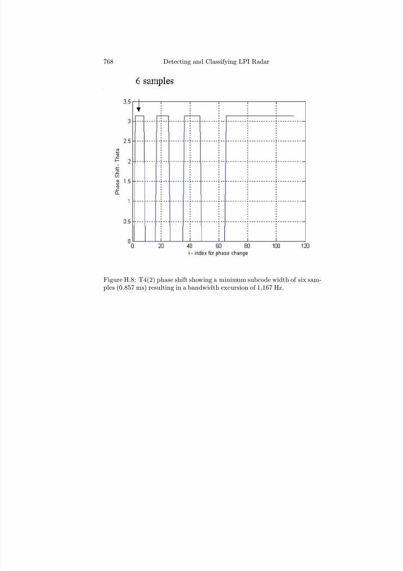
7/17/2019 1596932341 Intercept Radar.pdf
http://slidepdf.com/reader/full/1596932341-intercept-radarpdf 799/891
768 Detecting and Classifying LPI Radar
Figure H.8: T4(2) phase shift showing a minimum subcode width of six sam-ples (0.857 ms) resulting in a bandwidth excursion of 1,167 Hz.
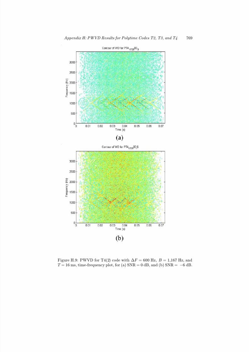
7/17/2019 1596932341 Intercept Radar.pdf
http://slidepdf.com/reader/full/1596932341-intercept-radarpdf 800/891
Appendix H: PWVD Results for Polytime Codes T2, T3, and T4 769
Figure H.9: PWVD for T4(2) code with ∆F = 600 Hz, B = 1,167 Hz, andT = 16 ms, time-frequency plot, for (a) SNR = 0 dB, and (b) SNR = −6 dB.

7/17/2019 1596932341 Intercept Radar.pdf
http://slidepdf.com/reader/full/1596932341-intercept-radarpdf 801/891

7/17/2019 1596932341 Intercept Radar.pdf
http://slidepdf.com/reader/full/1596932341-intercept-radarpdf 802/891
Appendix I
QMFB Results for FMCW
with ∆F = 500 Hz
In Figure I.1, the tm is increased from tm = 20 ms to tm = 30 ms, and thebandwidth is increased from ∆F = 250 Hz to ∆F = 500 Hz. Figure 10.19(a),shows layer l = 2. The same general characteristics are shown as in FigureI.1(a) except that fewer zeros are needed to pad the signal to N p = 2,048. InFigure I.1(b) the l = 5 layer is shown with ∆F = 112.9 Hz and ∆t = 4.64 ms< tm/6. That is, this layer provides a finer detail in time, and less detail infrequency. The bandwidth of the signal can easily be estimated as shown.
771

7/17/2019 1596932341 Intercept Radar.pdf
http://slidepdf.com/reader/full/1596932341-intercept-radarpdf 803/891
772 Detecting and Classifying LPI Radar
Figure I.1: QMFB time-frequency contour images for FMCW ∆F = 500MHz, tm = 30 ms (signal only), showing (a) layer 2, and (b) layer 5.

7/17/2019 1596932341 Intercept Radar.pdf
http://slidepdf.com/reader/full/1596932341-intercept-radarpdf 804/891
Appendix J
QMFB Results for 11-Bit
BPSK
An 11-bit Barker code (cpp = 1) is examined with the QMFB in Figure J.1.In Figure J.1(a), the full contour QMFB output for layer l = 3 is shown. InFigure J.1(b) a close-up view of the QMFB layer 3 output is shown, illustrat-ing the time changing frequency detail. Note the similarity in the structureof the frequency information when compared to Figure 10.21. Also note themajor diff erences in the frequency structure.
Figure J.2 shows the QMFB output contour of the 11-bit signal for bothlayers 3 and 6 for an SNR = 0 dB. Note that some of the features suchas bandwidth can be estimated but, even with a closer view of the results,information such as the phase is hard to determine.
In Figure J.3, the bandwidth of the 11-bit signal is narrowed from 1 kHz
to B = 0.2 kHz (code period of T = 55 ms). Figure J.3(a) shows the QMFBlayer 2 for two code periods. The presence of a null at each BPSK phase shiftis evident. With T = 55 ms, the measurement of the smallest subphase codeis performed, to determine the number of subphase codes contained withineach section of the code. Figure J.3(b) shows the QMFB layer 6. The codeperiod T and bandwidth B are clearly identified. Comparison with Figure10.23 indicates a slightly diff erent form, due to the additional subphase codes.
773

7/17/2019 1596932341 Intercept Radar.pdf
http://slidepdf.com/reader/full/1596932341-intercept-radarpdf 805/891
774 Detecting and Classifying LPI Radar
Figure J.1: QMFB layer 3 for BPSK with 11-bit Barker code, cpp = 1 (signalonly), showing (a) the full contour image, and (b) a close-up view showingfrequency details of Barker code.

7/17/2019 1596932341 Intercept Radar.pdf
http://slidepdf.com/reader/full/1596932341-intercept-radarpdf 806/891
Appendix J: QMFB Results for 11-Bit BPSK 775
Figure J.2: QMFB contour image for BPSK with 11-bit Barker code, cpp = 1(SNR = 0 dB), showing (a) layer 3, and (b) layer 6.

7/17/2019 1596932341 Intercept Radar.pdf
http://slidepdf.com/reader/full/1596932341-intercept-radarpdf 807/891
776 Detecting and Classifying LPI Radar
Figure J.3: QMFB contour images for BPSK 11-bit Barker code, cpp = 5(signal only), showing (a) layer 2, and (b) layer 6.

7/17/2019 1596932341 Intercept Radar.pdf
http://slidepdf.com/reader/full/1596932341-intercept-radarpdf 808/891
Appendix K
QMFB Results for Frank
Signal with N c = 16
The Frank code for M = 4 is shown in Figure K.1. The M = 4 Frank codesignal has N c = 16 subcodes, f c = 1 kHz, and a cpp = 1. The QMFBl = 2 layer for this signal is shown in Figure K.2 (∆f = 1,166.67 Hz, ∆t =573.67μs). The QMFB has 10 layers (N p = 1,024). Figure K.2(a) shows theentire signal (80 ms) and reveals that five code periods have been captured.Note the unique structure of the phase modulation. A closer examination isshown in Figure K.2(b). The code period (T = 16 ms) is shown, along withthe phase modulation characteristics due to the 16 subcodes. Correlation of the frequency characteristics within the code period shown in Figure K.2(b),with the phase modulation waveform shown in Figure K.1, can be madedirectly (four sections).
In Figure K.3(a) and (b), the QMFB l = 4 layer is shown (∆f = 233.33Hz, ∆t = 2.32 ms), and reveals the linear frequency modulation that results
from the Frank phase code. The bandwidth is also indicated. Note thatthe Frank code phase modulation results in the linear frequency modulationwrapping around for the i = 3 and i = 4 segment, starting at t = 40 ms.
777
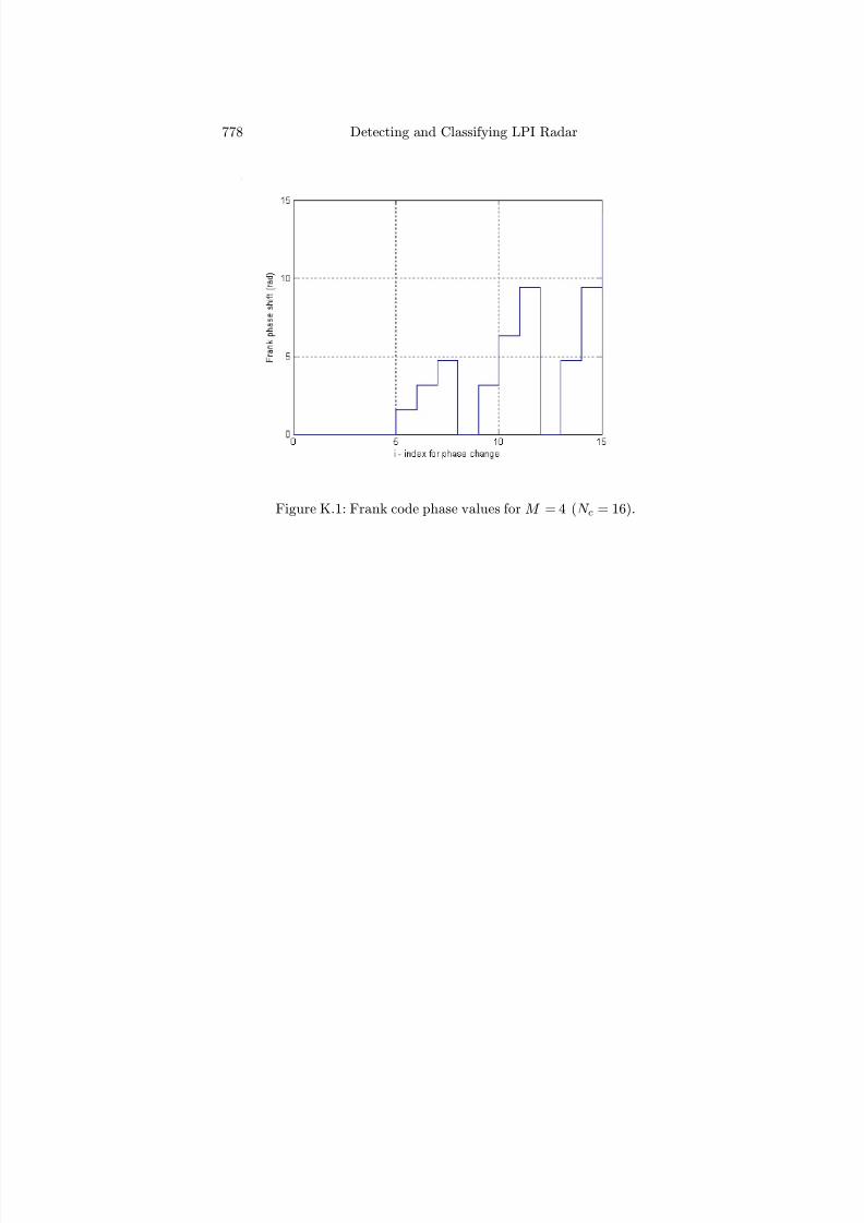
7/17/2019 1596932341 Intercept Radar.pdf
http://slidepdf.com/reader/full/1596932341-intercept-radarpdf 809/891
778 Detecting and Classifying LPI Radar
Figure K.1: Frank code phase values for M = 4 (N c = 16).
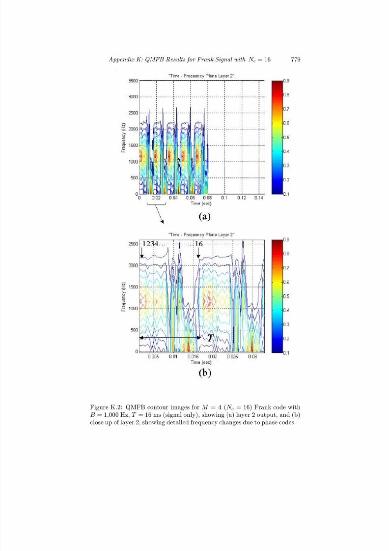
7/17/2019 1596932341 Intercept Radar.pdf
http://slidepdf.com/reader/full/1596932341-intercept-radarpdf 810/891
Appendix K: QMFB Results for Frank Signal with N c = 16 779
Figure K.2: QMFB contour images for M = 4 (N c = 16) Frank code withB = 1,000 Hz, T = 16 ms (signal only), showing (a) layer 2 output, and (b)close up of layer 2, showing detailed frequency changes due to phase codes.

7/17/2019 1596932341 Intercept Radar.pdf
http://slidepdf.com/reader/full/1596932341-intercept-radarpdf 811/891
780 Detecting and Classifying LPI Radar
Figure K.3: QMFB contour images for M = 4 Frank code with B = 1,000Hz, T = 16 ms (signal only), showing (a) layer 4 output, and (b) close up of layer 4, showing resulting linear frequency modulation.

7/17/2019 1596932341 Intercept Radar.pdf
http://slidepdf.com/reader/full/1596932341-intercept-radarpdf 812/891
Appendix L
QMFB Results for P1, P2,
P3, and P4
L.1 P1 Analysis
The P1 signal is also derived from a linear FM waveform. In this section itis shown that the P1 QMFB time-frequency characteristics are diff erent fromthe Frank code, and these diff erences can be used for waveform identification.In Figure L.1 the phase code for a P1 N c = 64 signal is shown for reference.The QMFB l = 2 layer is shown in Figure L.2. The total number of pointsshown are N p = 4,096 with L = 12 QMFB layers, ∆f = 1,166.67 Hz, and∆t = 571.99 μs. Since the number of phase codes is N c = 64, the five codeperiods extend for 320 ms. In the close-up view of the code period in FigureL.2(b), the variation in phase modulation characteristics can be identified and
correlated with the phase waveform given above. This is especially evidentfor the last four sections given in Figure L.1.
In Figure L.3(a) and (b), the l = 5 layer is shown, demonstrating thelinear frequency modulation resulting from the P1 phase codes. For this layer,∆f = 112.9 Hz and ∆t = 4.61 ms. Note the immediate frequency wraparoundat the beginning of the code period. Also evident is the nonuniform spacingof the energy concentrations, due to the nonlinear phase modulation. Thecode period (T = 64 ms) and bandwidth B = 1,000 Hz are also shown.The marginal frequency characteristics for the N c = 64 P1 code are shownin Figure L.4. Due to the nonlinear phase modulation characteristics, theenergy is not symmetrically distributed about filter 9 (the carrier frequencyf c = 1 kHz). From Figure L.4 the four largest energy tiles (in order fromlargest to smallest) are 7, 8, 10, and 9. That is, the carrier has the smallest
amount of energy among the four largest components.
781

7/17/2019 1596932341 Intercept Radar.pdf
http://slidepdf.com/reader/full/1596932341-intercept-radarpdf 813/891
782 Detecting and Classifying LPI Radar
Figure L.1: P1 code phase values for N c = 64.
L.2 P2 Analysis
The P2 phase modulation diagram for N c = 64 phase codes is shown in FigureL.5. This phase diagram has a particularly interesting shape, giving rise tosome unique characteristics in the time-frequency domain.
The QMFB for the signal shown in this example has L = 12 layers. InFigure L.6, the contour images for QMFB layer 2 are shown with ∆f =1,166.67 Hz and ∆t = 571.99 μs. The pattern of the frequency characteristicschanges form toward the middle of the code period (T = 40 ms). The resultis a linear frequency modulation that has a negative slope . This is illustratedin Figure L.7, which shows the l = 5 layer. For this layer, ∆f = 112.9 Hz and∆t = 4.61 ms. Note from Figure L.7(b), the four energy concentrations arelocated toward the center of the code period. Diff erent signal modulationswill have distinct levels of energy concentration. Consequently, the marginalfrequency distribution can be used to identify the signal’s modulation type.Figure L.8 shows the QMFB layer 5 marginal frequency profile for the N c = 64P2 code. From Figure L.8 the four largest energy tiles (in order from largestto smallest) are 7, 9, 8, and 10. The diff erence between the P1 and P2 codecan be identified by comparing marginal frequency distributions shown inFigure L.8 and Figure L.4.
L.3 P3 Analysis
The P3 phase modulation for N c = 64 (64 phase codes) is shown for reference
in Figure L.9. The QMFB l = 2 layer for the P3 signal is shown in FigureL.10. The contour images are shown with ∆f = 1,166.67 Hz and ∆t = 571.99

7/17/2019 1596932341 Intercept Radar.pdf
http://slidepdf.com/reader/full/1596932341-intercept-radarpdf 814/891
Appendix L: QMFB Results for P1, P2, P3, and P4 783
Figure L.2: QMFB contour images for N c = 64 P1 code with B = 1,000 Hz,T = 64 ms (signal only), showing (a) layer 2 output and (b) close up of layer2, showing detailed frequency changes due to phase codes.

7/17/2019 1596932341 Intercept Radar.pdf
http://slidepdf.com/reader/full/1596932341-intercept-radarpdf 815/891
784 Detecting and Classifying LPI Radar
Figure L.3: QMFB contour images for N c = 64 P1 code with B = 1,000 Hz,T = 64 ms (signal only), showing (a) layer 5 output, and (b) close up of layer5, showing resulting linear frequency modulation.

7/17/2019 1596932341 Intercept Radar.pdf
http://slidepdf.com/reader/full/1596932341-intercept-radarpdf 816/891
Appendix L: QMFB Results for P1, P2, P3, and P4 785
Figure L.4: QMFB layer 5 marginal frequency profile for N c = 64 P1 code.
Figure L.5: P2 code phase values for N c = 64.
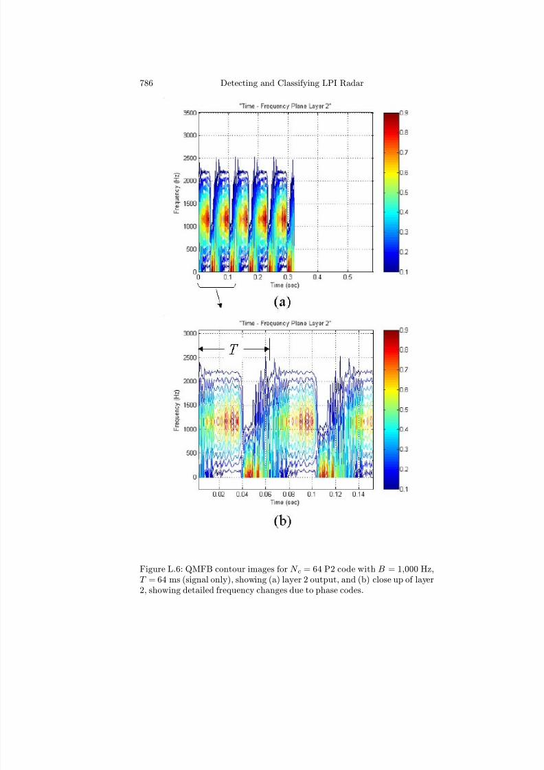
7/17/2019 1596932341 Intercept Radar.pdf
http://slidepdf.com/reader/full/1596932341-intercept-radarpdf 817/891
786 Detecting and Classifying LPI Radar
Figure L.6: QMFB contour images for N c = 64 P2 code with B = 1,000 Hz,T = 64 ms (signal only), showing (a) layer 2 output, and (b) close up of layer2, showing detailed frequency changes due to phase codes.
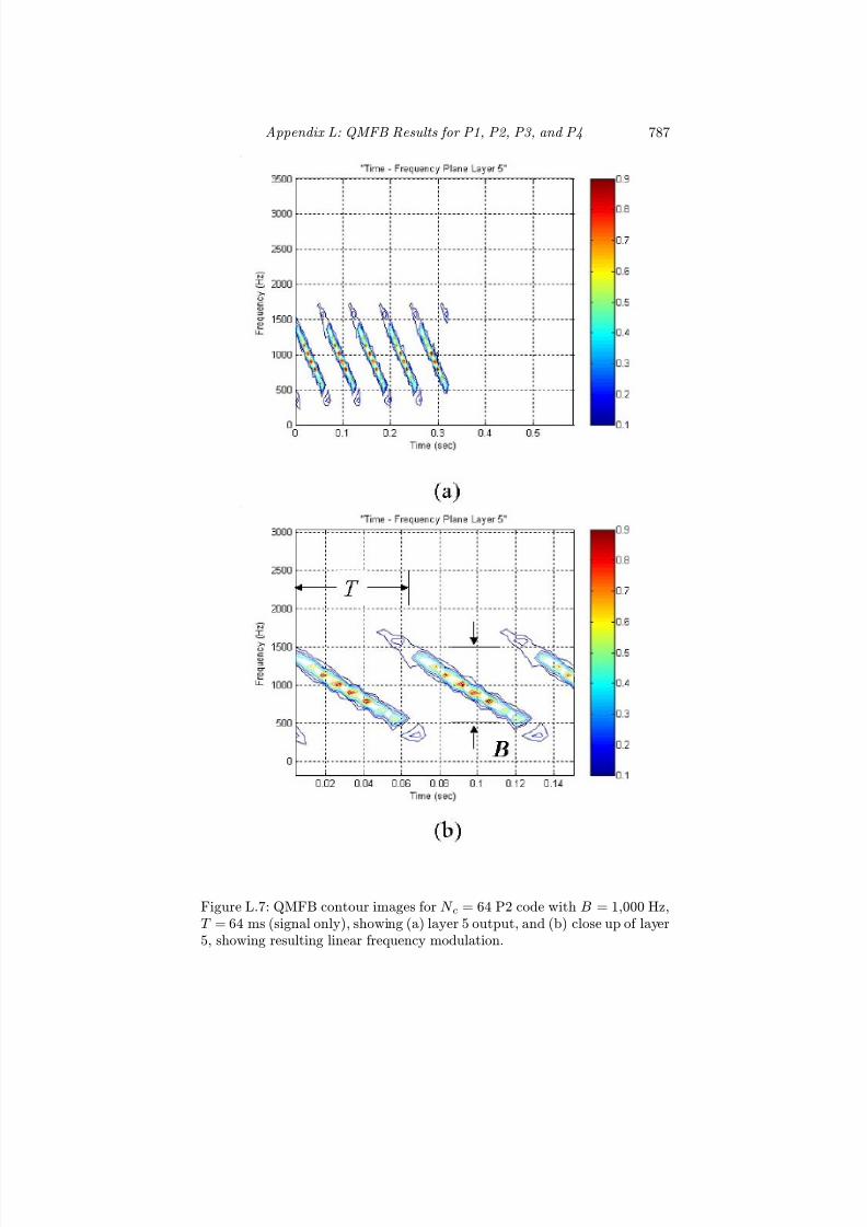
7/17/2019 1596932341 Intercept Radar.pdf
http://slidepdf.com/reader/full/1596932341-intercept-radarpdf 818/891
Appendix L: QMFB Results for P1, P2, P3, and P4 787
Figure L.7: QMFB contour images for N c = 64 P2 code with B = 1,000 Hz,T = 64 ms (signal only), showing (a) layer 5 output, and (b) close up of layer5, showing resulting linear frequency modulation.

7/17/2019 1596932341 Intercept Radar.pdf
http://slidepdf.com/reader/full/1596932341-intercept-radarpdf 819/891
788 Detecting and Classifying LPI Radar
Figure L.8: QMFB layer 5 marginal frequency profile for N c = 64 P2 code.
μs. The shape of the time-frequency characteristics is unique from those of the Frank, P1, and P2 codes.
Figure L.11 shows the l = 5 layer indicating the bandwidth and codeperiod. Here ∆f = 112.9 Hz and ∆t = 4.61 ms. A closer examination of thelayer 5 frequency details reveal a diff erent distribution of the energy peakswithin the bandwidth. The marginal frequency distribution for the P3 codeis shown in Figure L.12. From Figure L.12 the four largest energy tiles (inorder from largest to smallest) are 7, 9, 10, and 8. Again, this is distinctfrom the Frank, P1, and P2 codes and can be used to classify the detectedP3 signal.
L.4 P4 Analysis
In this section, an N c = 64 P4 code is examined with the QMFB. The P4phase modulation for N c = 64 is shown in Figure L.13. The QMFB forthis P4 signal has L = 12 layers. The l = 2 layer (∆f = 1,166.67 Hz and∆t = 571.99 μs) is shown in Figure L.14. The close-up view examines thetime-varying frequency characteristics of the signal as it appears within twoof the three filters. Figure L.15 shows the l = 5 layer (∆f = 112.9 Hz and∆t = 4.61), demonstrating the P4 linear frequency modulation. The close-upview shows the major energy peaks about the carrier frequency (ninth filter).For the P4 code, the marginal frequency distribution shown in Figure L.16,
reveals that the largest energy concentration is at the carrier frequency . thefour largest energy tiles (in order from largest to smallest) are 9, 7, 10, and8.

7/17/2019 1596932341 Intercept Radar.pdf
http://slidepdf.com/reader/full/1596932341-intercept-radarpdf 820/891
Appendix L: QMFB Results for P1, P2, P3, and P4 789
Figure L.9: P3 code phase values for N c = 64.

7/17/2019 1596932341 Intercept Radar.pdf
http://slidepdf.com/reader/full/1596932341-intercept-radarpdf 821/891
790 Detecting and Classifying LPI Radar
Figure L.10: QMFB contour images for N c = 64 P3 code with B = 1,000 Hz,T = 64 ms (signal only), showing (a) layer 2 output, and (b) close up of layer2, showing detailed frequency changes due to phase codes.
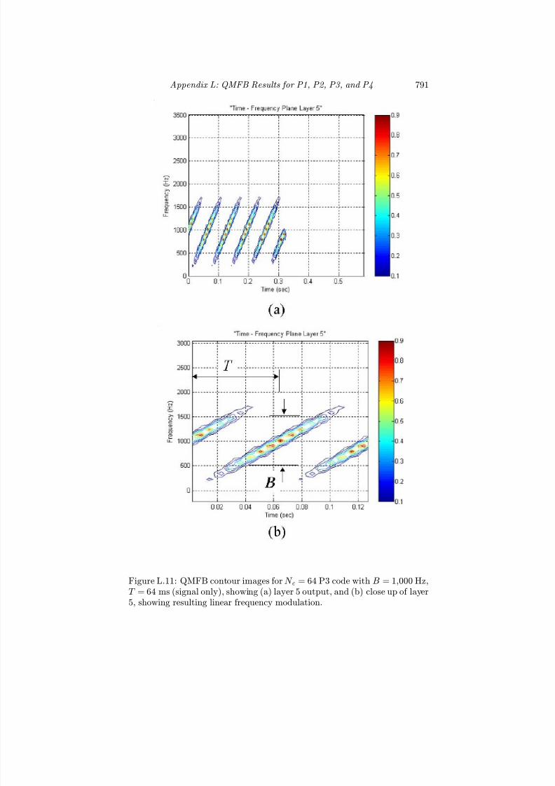
7/17/2019 1596932341 Intercept Radar.pdf
http://slidepdf.com/reader/full/1596932341-intercept-radarpdf 822/891
Appendix L: QMFB Results for P1, P2, P3, and P4 791
Figure L.11: QMFB contour images for N c = 64 P3 code with B = 1,000 Hz,T = 64 ms (signal only), showing (a) layer 5 output, and (b) close up of layer5, showing resulting linear frequency modulation.

7/17/2019 1596932341 Intercept Radar.pdf
http://slidepdf.com/reader/full/1596932341-intercept-radarpdf 823/891
792 Detecting and Classifying LPI Radar
Figure L.12: QMFB layer 5 marginal frequency profile for N c = 64 P3 code.
Figure L.13: P4 code phase values for N c = 64.

7/17/2019 1596932341 Intercept Radar.pdf
http://slidepdf.com/reader/full/1596932341-intercept-radarpdf 824/891
Appendix L: QMFB Results for P1, P2, P3, and P4 793
Figure L.14: QMFB contour images for N c = 64 P4 code with B = 1,000 Hz,T = 64 ms (signal only), showing (a) layer 2 output, and (b) close up of layer2, showing detailed frequency changes due to phase codes.

7/17/2019 1596932341 Intercept Radar.pdf
http://slidepdf.com/reader/full/1596932341-intercept-radarpdf 825/891
794 Detecting and Classifying LPI Radar
Figure L.15: QMFB contour images for N c = 64 P4 code with B = 1,000 Hz,T = 64 ms (signal only), showing (a) layer 5 output, and (b) close up of layer5, showing resulting linear frequency modulation.

7/17/2019 1596932341 Intercept Radar.pdf
http://slidepdf.com/reader/full/1596932341-intercept-radarpdf 826/891
Appendix L: QMFB Results for P1, P2, P3, and P4 795
Figure L.16: QMFB layer 5 marginal frequency profile for N c = 64 P4 code.

7/17/2019 1596932341 Intercept Radar.pdf
http://slidepdf.com/reader/full/1596932341-intercept-radarpdf 827/891

7/17/2019 1596932341 Intercept Radar.pdf
http://slidepdf.com/reader/full/1596932341-intercept-radarpdf 828/891
Appendix M
QMFB Results for T2, T3,
and T4
Figure M.1(a) and Figure M.1(b) show the QMFB contour images for thepolytime T2(2) code with B = 875 Hz and T = 16 ms, showing the layer 2output. The code modulation period is indicated, and the number of codeperiods can also be identified. The close-up in Figure M.1(b) shows the uniquetime-frequency pattern due to the T2(2) phase modulation. Figure M.2(a)and Figure M.2(b) show the QMFB contour images for the polytime T2(2)code with B = 875 Hz and T = 16 ms, showing the layer 4 output. Note thebandwidth and code period can easily be indentified.
In Figure M.3(a) and (b), the QMFB contour images for the polytimeT3(2) code with B = 1,167 Hz, T = 16 ms (signal only) are shown. InFigure M.3(a) the layer 2 output is shown, and in Figure M.3(b) a close-up of
layer 2 is used to indicate the frequency changes due to the phase codes. InFigure M.4, layer 4 is examined, and shows the bipolar frequency modulationcharacteristic of the T3(2) code. Also indicated are the bandwidth and codeperiod.
Layer 2 for the T4(2) code is shown in Figure M.5. All five code periodsare shown, as well as the code period of 16 ms. Layer 4 is shown in FigureM.6. Interestingly enough, all of the polytime codes have a large frequencyspike within each code period, due to the recycling of the phase modulation.
797

7/17/2019 1596932341 Intercept Radar.pdf
http://slidepdf.com/reader/full/1596932341-intercept-radarpdf 829/891
798 Detecting and Classifying LPI Radar
Figure M.1: QMFB contour images for polytime T2(2) code with B = 875Hz, T = 16 ms (signal only), showing (a) layer 2 output, and (b) close-up of layer 2, showing detailed frequency changes due to phase codes.

7/17/2019 1596932341 Intercept Radar.pdf
http://slidepdf.com/reader/full/1596932341-intercept-radarpdf 830/891
Appendix M: QMFB Results for T2, T3, and T4 799
Figure M.2: QMFB contour images for polytime T2(2) code with B = 875Hz, T = 16 ms (signal only), showing (a) layer 4 output, and (b) close-up of layer 4, showing resulting linear frequency modulation.
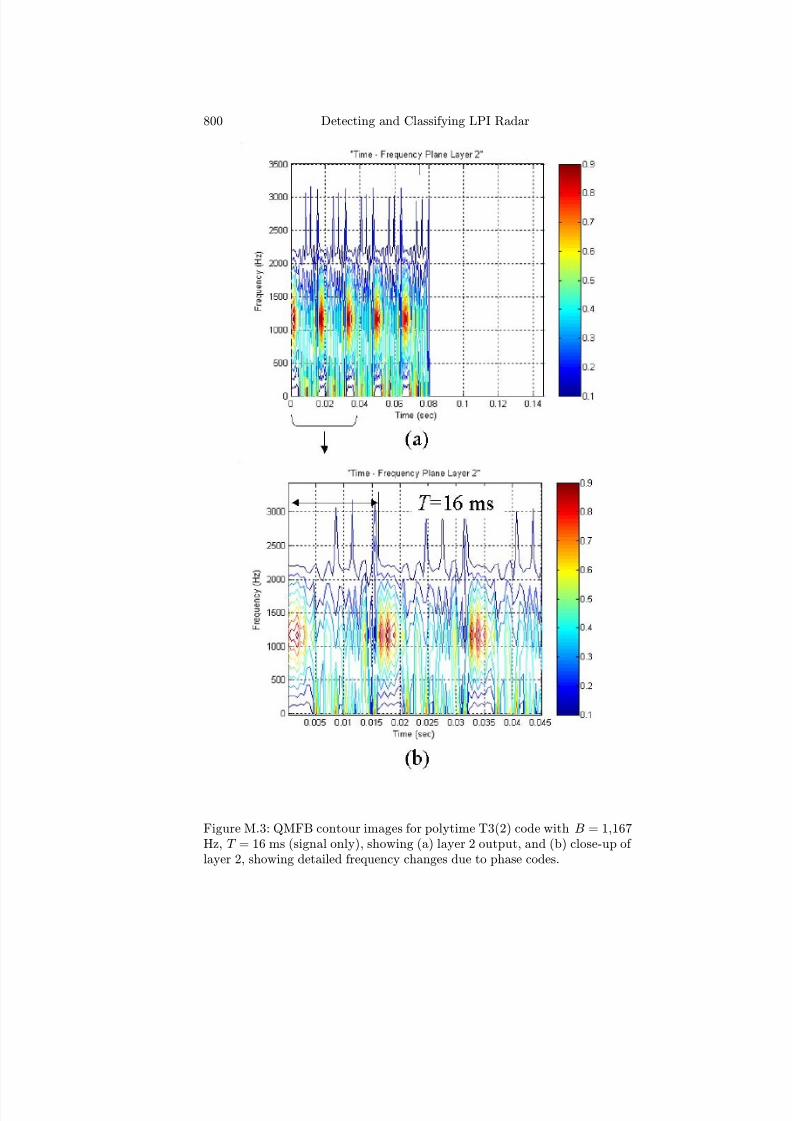
7/17/2019 1596932341 Intercept Radar.pdf
http://slidepdf.com/reader/full/1596932341-intercept-radarpdf 831/891
800 Detecting and Classifying LPI Radar
Figure M.3: QMFB contour images for polytime T3(2) code with B = 1,167Hz, T = 16 ms (signal only), showing (a) layer 2 output, and (b) close-up of layer 2, showing detailed frequency changes due to phase codes.

7/17/2019 1596932341 Intercept Radar.pdf
http://slidepdf.com/reader/full/1596932341-intercept-radarpdf 832/891
Appendix M: QMFB Results for T2, T3, and T4 801
Figure M.4: QMFB contour images for polytime T3(2) code with B = 1,167Hz, T = 16 ms (signal only), showing (a) layer 4 output, and (b) close-up of layer 4, showing resulting linear frequency modulation.
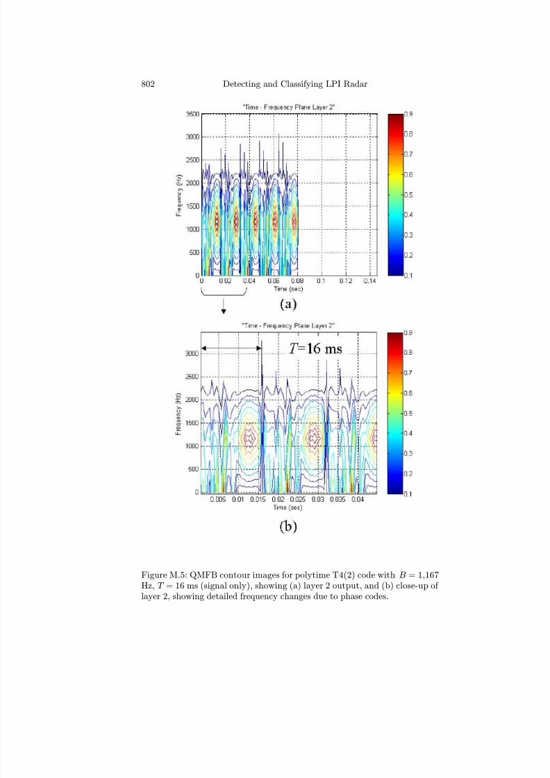
7/17/2019 1596932341 Intercept Radar.pdf
http://slidepdf.com/reader/full/1596932341-intercept-radarpdf 833/891
802 Detecting and Classifying LPI Radar
Figure M.5: QMFB contour images for polytime T4(2) code with B = 1,167Hz, T = 16 ms (signal only), showing (a) layer 2 output, and (b) close-up of layer 2, showing detailed frequency changes due to phase codes.

7/17/2019 1596932341 Intercept Radar.pdf
http://slidepdf.com/reader/full/1596932341-intercept-radarpdf 834/891
Appendix M: QMFB Results for T2, T3, and T4 803
Figure M.6: QMFB contour images for polytime T4(2) code with B = 1,167Hz, T = 16 ms (signal only), showing (a) layer 4 output, and (b) close-up of layer 4, showing resulting linear frequency modulation.

7/17/2019 1596932341 Intercept Radar.pdf
http://slidepdf.com/reader/full/1596932341-intercept-radarpdf 835/891
7/17/2019 1596932341 Intercept Radar.pdf
http://slidepdf.com/reader/full/1596932341-intercept-radarpdf 836/891
Appendix N
Cyclostationary Processing
Results with FMCW
∆F = 500 Hz
The extraction of the parameters from a wideband FMCW signal ∆F = 500Hz using cyclostationary processing is not significantly diff erent, and is shownin Figure N.1. The modulation period for this example tm = 30 ms. FigureN.1(a) shows the modulation pattern with centroid at 2f c = 2 kHz. Notethat the arrowhead pattern unique to the FMCW is still present, but hasa bit more structure. With this resolution, ∆F can easily be measured;however, Rc cannot be measured. The closer examination shown in FigureN.1(b) reveals the unique modulation characteristic of the FMCW waveform.
The value of Rc = 16.7 Hz is now easily identifi
ed giving a tm = 30 ms.The SNR = 0 dB case is shown in Figure N.2(a) and (b). Note that thecyclostationary results are fairly robust in significant amounts of noise.
805
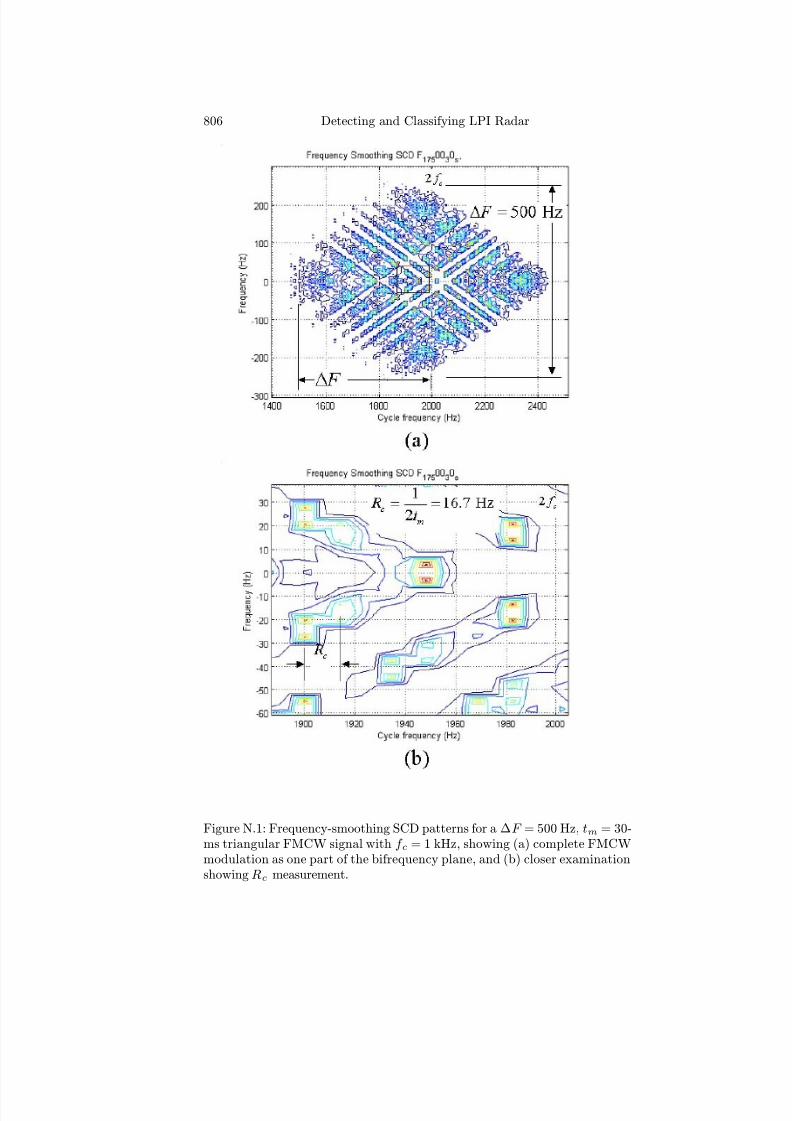
7/17/2019 1596932341 Intercept Radar.pdf
http://slidepdf.com/reader/full/1596932341-intercept-radarpdf 837/891

7/17/2019 1596932341 Intercept Radar.pdf
http://slidepdf.com/reader/full/1596932341-intercept-radarpdf 838/891
Appendix N: Cyclostationary Results with FMCW ∆F = 500 Hz 807
Figure N.2: Frequency-smoothing SCD patterns for a ∆F = 500 Hz, tm = 30-ms triangular FMCW signal with f c = 1 kHz, showing (a) the bifrequencyplane with SNR = 0 dB, and (b) closer examination showing Rc measurement.

7/17/2019 1596932341 Intercept Radar.pdf
http://slidepdf.com/reader/full/1596932341-intercept-radarpdf 839/891

7/17/2019 1596932341 Intercept Radar.pdf
http://slidepdf.com/reader/full/1596932341-intercept-radarpdf 840/891
Appendix O
Cyclostationary Processing
Results with Frank Signal,
N c = 16
For the signal examined, f c = 1 kHz, cpp = 1, f s = 7 kHz, and N c = 16phase subcodes. The frequency-smoothing SCD is generated using ∆k = 16Hz with N = 1,024. One of the four modulation patterns generated in theSCD is shown in Figure O.1(a). As in previous examples, the pattern centroidis located at γ = 2f c. For the Frank code this is a bit more difficult to identify,due to the diff erent slopes of phase shift within each single code period T .Generally, it lies in the center of the cross-hatch area inside the lesser SCDamplitude (faded) regions. That is, the cross-hatch region of interest is not
symmetrical about the centroid. Location of the centroid can be used todetermine the bandwidth on the cycle frequency axis, but there is a morestraightforward method for determining the bandwidth in the bifrequencyplane. To do this we first outline the cross-hatch region (larger amplitudeSCD) with a parallelogram (shown by dashed lines). The top and bottomcorners of the parallelogram are colocated at the same cycle frequency, andthe left and right corners are colocated at the same frequency (f = 0). Thisinformation helps identify the parallelogram position, and the bandwidth Bcan be estimated more accurately. For the Frank code, the Rc measurementis related to the code period as Rc = 1/T = 1/N ctb. In Figure O.1(b), a closerexamination shows that the Rc measurement is straightforward, and for thissignal Rc = 62.5 Hz. The number of subcodes within a code period is thenN c = B/Rc = 16. Figure O.2 shows the bifrequency analysis for the Frank
code in the presence of noise. In Figure O.2(a), the Frank code modulation is
809
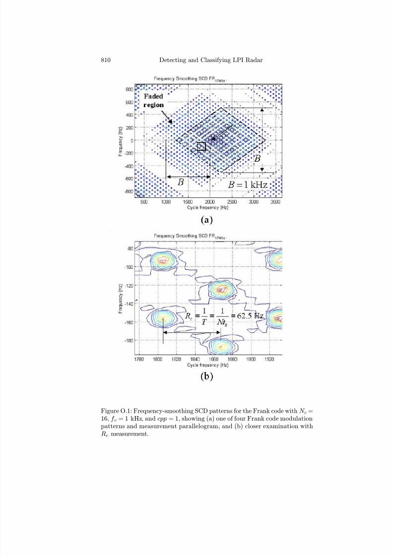
7/17/2019 1596932341 Intercept Radar.pdf
http://slidepdf.com/reader/full/1596932341-intercept-radarpdf 841/891
810 Detecting and Classifying LPI Radar
Figure O.1: Frequency-smoothing SCD patterns for the Frank code with N c =16, f c = 1 kHz, and cpp = 1, showing (a) one of four Frank code modulationpatterns and measurement parallelogram, and (b) closer examination withRc measurement.
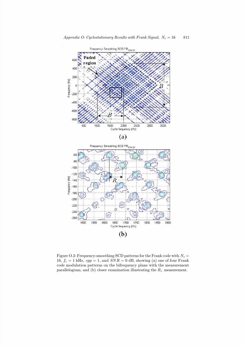
7/17/2019 1596932341 Intercept Radar.pdf
http://slidepdf.com/reader/full/1596932341-intercept-radarpdf 842/891
Appendix O: Cyclostationary Results with Frank Signal, N c = 16 811
Figure O.2: Frequency-smoothing SCD patterns for the Frank code with N c =16, f c = 1 kHz, cpp = 1, and SNR = 0 dB, showing (a) one of four Frankcode modulation patterns on the bifrequency plane with the measurementparallelogram, and (b) closer examination illustrating the Rc measurement.

7/17/2019 1596932341 Intercept Radar.pdf
http://slidepdf.com/reader/full/1596932341-intercept-radarpdf 843/891
812 Detecting and Classifying LPI Radar
shown with an SNR = 0 dB. Note the position of the parallelogram to enclosethe cross-hatch region. Also note the corner locations and the bandwidthmeasurement. Figure O.2(b) shows the Rc measurement. In summary, theunique pattern of the wideband Frank code lets us determine all of the signalparameters using the SCD bifrequency plane.

7/17/2019 1596932341 Intercept Radar.pdf
http://slidepdf.com/reader/full/1596932341-intercept-radarpdf 844/891
Appendix P
Cyclostationary Processing
Results for P1, P2, P3,
and P4
P.1 P1 Code Analysis
In this section we investigate the time-smoothing SCD for the P1 signal,and illustrate the corresponding extraction technique. The signal examinedis a P1 phase-modulated signal with f c = 1 kHz, N c = 64 subcodes, andcpp = 1 (wideband). Figure P.1(a) shows the complete bifrequency plane, andreveals that the P1 code also presents itself in an insect pattern. Comparedto the Frank code signal, however, note that the insect is pointed to the left.
This is expected, since the time-frequency slope as measured by the Wignerdistribution and quadrature mirror filtering is opposite to that of the Frankcode. As illustrated in Figure P.1(b), the bandwidth is measured on the cyclefrequency axis in a similar fashion to the Frank code, except that the headis on the left. Correlation with the frequency axis measurement of B is alsoillustrated.
Also indicated in Figure P.1(b) is a box that is examined in closer detail toillustrate the Rc measurement. Figure P.2(a) and (b) illustrate the measure-ment of Rc = 1/T . Figure P.2(b) indicates Rc = 15.5 Hz, giving a modulationperiod of 64 ms. Again, since the number of subcodes used by LPI radar aremost often a power of 2 (e.g., 64 = 26), an accurate result can be obtainedeven from a bifrequency plane with small SNR. Here N c = B/Rc = 64.
813
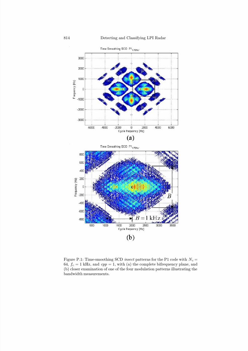
7/17/2019 1596932341 Intercept Radar.pdf
http://slidepdf.com/reader/full/1596932341-intercept-radarpdf 845/891
814 Detecting and Classifying LPI Radar
Figure P.1: Time-smoothing SCD insect patterns for the P1 code with N c =64, f c = 1 kHz, and cpp = 1, with (a) the complete bifrequency plane, and(b) closer examination of one of the four modulation patterns illustrating thebandwidth measurements.

7/17/2019 1596932341 Intercept Radar.pdf
http://slidepdf.com/reader/full/1596932341-intercept-radarpdf 846/891
Appendix P: Cyclostationary Results for P1, P2, P3, and P4 815
Figure P.2: Close examination of time-smoothing SCD for the P1 code withN c = 64, f c = 1 kHz, and cpp = 1, with (a) modulation cycles, and (b) themeasurement of Rc.

7/17/2019 1596932341 Intercept Radar.pdf
http://slidepdf.com/reader/full/1596932341-intercept-radarpdf 847/891
816 Detecting and Classifying LPI Radar
P.2 P2 Code Analysis
The time-smoothing SCD results for the P2 code are illustrated in Figure
P.3(a). The P2 modulation has the expected insect shape, however, it ispointing to the right (similar to the Frank code). Note also the distinct nullspresent in the bifrequency. The bandwidth is measured in a similar mannerto the P1 and Frank code; however, the bifrequency nulls must be used asillustrated in Figure P.3(b). One advantage of using the bifrequency planefor measuring Rc for the subcode period tb and number of subcodes N is thenonspecific position in the bifrequency plane, where Rc can be measured. Asshown in Figure P.4(a) and (b), any (γ , k) region can be used to estimate thevalue of Rc.
P.3 P3 Code Analysis
The time-smoothing SCD results for the P3 code are shown in Figure P.5.The signal has f c = 1 kHz, N c = 64 (64 subcodes), and cpp = 1. The insectmodulation pattern points to the right and the measurements of B and Rc,as well as N and cpp, are the same as the above cases.
P.4 P4 Code Analysis
The time-smoothing SCD results for the P4 code are shown in Figure P.6.The signal has f c = 1 kHz, N c = 64, and cpp = 1. The insect modulationpattern points to the right and the measurements of B and Rc, as well as N and cpp, are the same as above.
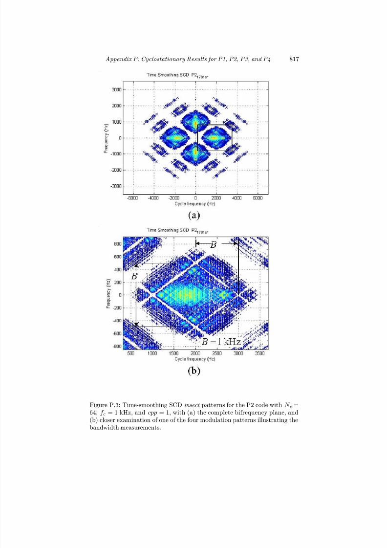
7/17/2019 1596932341 Intercept Radar.pdf
http://slidepdf.com/reader/full/1596932341-intercept-radarpdf 848/891
Appendix P: Cyclostationary Results for P1, P2, P3, and P4 817
Figure P.3: Time-smoothing SCD insect patterns for the P2 code with N c =64, f c = 1 kHz, and cpp = 1, with (a) the complete bifrequency plane, and(b) closer examination of one of the four modulation patterns illustrating thebandwidth measurements.
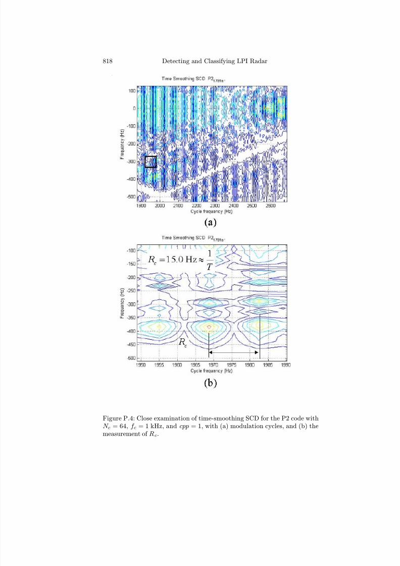
7/17/2019 1596932341 Intercept Radar.pdf
http://slidepdf.com/reader/full/1596932341-intercept-radarpdf 849/891
818 Detecting and Classifying LPI Radar
Figure P.4: Close examination of time-smoothing SCD for the P2 code withN c = 64, f c = 1 kHz, and cpp = 1, with (a) modulation cycles, and (b) themeasurement of Rc.
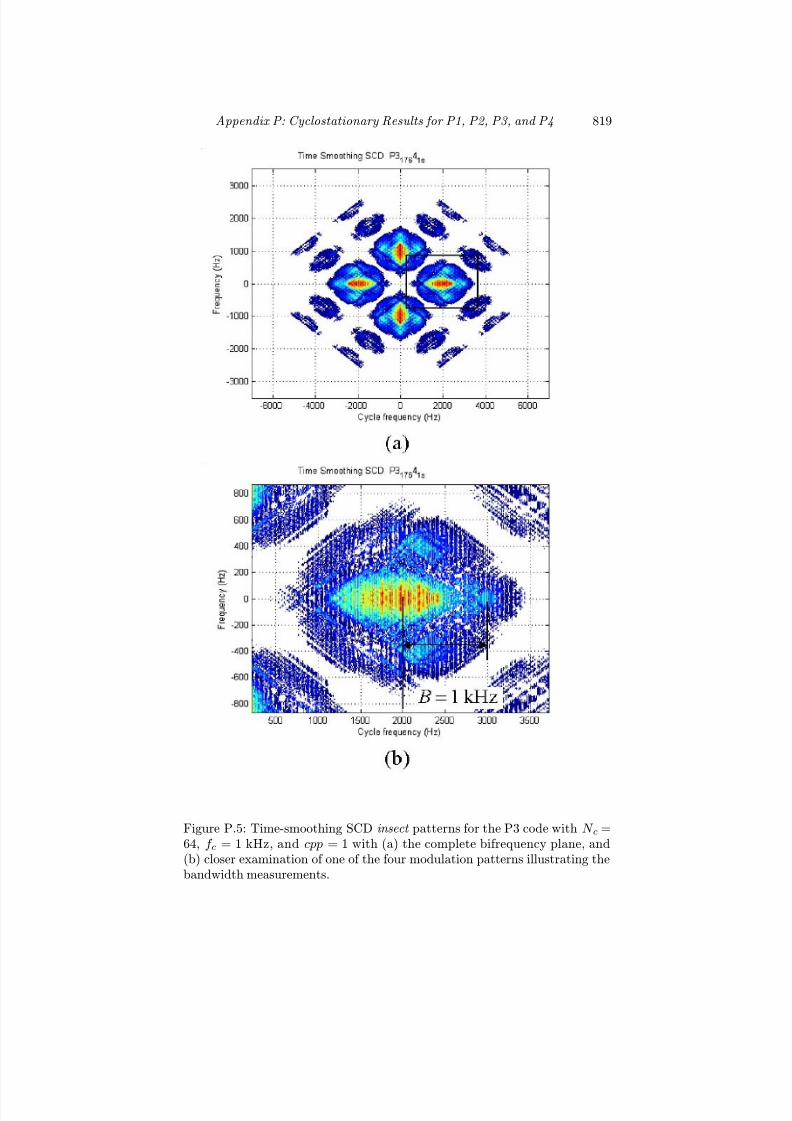
7/17/2019 1596932341 Intercept Radar.pdf
http://slidepdf.com/reader/full/1596932341-intercept-radarpdf 850/891
Appendix P: Cyclostationary Results for P1, P2, P3, and P4 819
Figure P.5: Time-smoothing SCD insect patterns for the P3 code with N c =64, f c = 1 kHz, and cpp = 1 with (a) the complete bifrequency plane, and(b) closer examination of one of the four modulation patterns illustrating thebandwidth measurements.

7/17/2019 1596932341 Intercept Radar.pdf
http://slidepdf.com/reader/full/1596932341-intercept-radarpdf 851/891
820 Detecting and Classifying LPI Radar
Figure P.6: Time-smoothing SCD insect patterns for the P4 code with N c =64, f c = 1 kHz, and cpp = 1 with (a) the complete bifrequency plane, and(b) closer examination of one of the four modulation patterns illustrating thebandwidth measurements.

7/17/2019 1596932341 Intercept Radar.pdf
http://slidepdf.com/reader/full/1596932341-intercept-radarpdf 852/891
Appendix Q
Cyclostationary ProcessingResults for T2, T3, and T4
Polytime Codes
Q.1 Polytime T2(2) Code Analysis
In this section, the frequency-smoothing SCD is used to examine the polytimeT2(2) code. The T2(2) code also has an f c = 1 kHz, and has a time-modulatedbinary phase shift (of various widths). Figure Q.1(a) shows the bifrequencyplane and the four modulation patterns. Figure Q.1(b) shows one of thefour unique patterns, and illustrates how the bandwidth of the signal canbe measured. Comparison with the T1(2) code shows that the bandwidth is
exactly one-half as large as in the T1(2) code. For the T2(2) signal shownin Figure Q.1(b), B = 875 Hz. Figure Q.2 shows a closer examination of thebifrequency plane, and the measurement of R
c = 1/T = 62.5 Hz. This gives
the estimate for the code period as T = 16 ms. Note also that an SCD spotdoes not exist at γ = 2f c, k = 0 and is an additional method to distinguishbetween the two bifrequency patterns.
Q.2 Polytime T3(2) Code Analysis
In this section, the frequency-smoothing SCD is used to examine the polytimeT3(2) code. The T3(2) code also has an f
c = 1 kHz, and has a time-modulated
binary phase shift (of various widths) across a modulation bandwidth ∆F =
600 Hz. Figure Q.3(a) shows the bifrequency plane and the four modulation
821

7/17/2019 1596932341 Intercept Radar.pdf
http://slidepdf.com/reader/full/1596932341-intercept-radarpdf 853/891
822 Detecting and Classifying LPI Radar
Figure Q.1: Frequency-smoothing SCD patterns for the polytime T2(2) codewith f c = 1 kHz, showing (a) the complete bifrequency plane, and (b) closerexamination of one of the four modulation patterns illustrating the bandwidthmeasurement.

7/17/2019 1596932341 Intercept Radar.pdf
http://slidepdf.com/reader/full/1596932341-intercept-radarpdf 854/891
Appendix Q: Cyclostationary Results for T2, T3, and T4 Codes 823
Figure Q.2: Close examination of the frequency-smoothing SCD pattern forthe polytime T2(2) code, illustrating the Rc measurement.
patterns. Figure Q.3(b) shows one of the four unique patterns. The distancefrom the centroid to the corner of the dot pattern on the k = 0 axis is 2∆F .For the T3(2) signal shown in Figure Q.3(b), ∆F = 600 Hz. Figure Q.4shows a closer examination of the bifrequency plane, and the measurement of Rc
= 1/T = 62.5 Hz. This also correctly gives the estimate for the code periodas T = 16 ms. Note also that an SCD spot does exist at (γ = 2f c, k = 0).
Q.3 Polytime T4(2) Code Analysis
In this section the frequency-smoothing SCD is used to examine the polytimeT4(2) code. The T4(2) code also has an f c = 1 kHz, and has a time-modulatedbinary phase shift (of various widths) across a modulation bandwidth ∆F =600 Hz. Figure Q.5(a) shows the bifrequency plane and the four modulationpatterns. Figure Q.5(b) shows one of the four unique patterns. The distancefrom the centroid to the corner of the dot pattern on the k = 0 axis is also2∆F . For the T4(2) signal shown in Figure Q.5(b), ∆F = 600 Hz. Figure Q.6shows a closer examination of the bifrequency plane, and the measurement of R
c = 1/T = 62.5 Hz. This also correctly gives the estimate for the code period
as T = 16 ms. Note also that an SCD spot does exist at (γ = 2f c, k = 0).

7/17/2019 1596932341 Intercept Radar.pdf
http://slidepdf.com/reader/full/1596932341-intercept-radarpdf 855/891
824 Detecting and Classifying LPI Radar
Figure Q.3: Frequency-smoothing SCD patterns for the polytime T3(2) codewith f c = 1 kHz showing (a) the complete bifrequency plane, and (b) closerexamination of one of the four modulation patterns illustrating the bandwidthmeasurement.

7/17/2019 1596932341 Intercept Radar.pdf
http://slidepdf.com/reader/full/1596932341-intercept-radarpdf 856/891
Appendix Q: Cyclostationary Results for T2, T3, and T4 Codes 825
Figure Q.4: Close examination of the frequency-smoothing SCD pattern forthe polytime T3(2) code, illustrating the Rc measurement.

7/17/2019 1596932341 Intercept Radar.pdf
http://slidepdf.com/reader/full/1596932341-intercept-radarpdf 857/891
826 Detecting and Classifying LPI Radar
Figure Q.5: Frequency-smoothing SCD patterns for the polytime T4(2) codewith f c = 1 kHz, showing (a) the complete bifrequency plane, and (b) closerexamination of one of the four modulation patterns illustrating the bandwidthmeasurement.

7/17/2019 1596932341 Intercept Radar.pdf
http://slidepdf.com/reader/full/1596932341-intercept-radarpdf 858/891
Appendix Q: Cyclostationary Results for T2, T3, and T4 Codes 827
Figure Q.6: Close examination of the frequency-smoothing SCD pattern forthe polytime T4(2) code, illustrating the Rc measurement.

7/17/2019 1596932341 Intercept Radar.pdf
http://slidepdf.com/reader/full/1596932341-intercept-radarpdf 859/891

7/17/2019 1596932341 Intercept Radar.pdf
http://slidepdf.com/reader/full/1596932341-intercept-radarpdf 860/891
List of Symbols
There are not enough symbols in the English and Greek alphabets to allow theuse of each letter or symbol once. Consequently, some symbols may be used todenote more than one variable, but their use should be clear from the context.
Symbols
a multiplying coefficients for envelope approximation detectorA complex leakage signalA signal amplitudeA Albersheim SNR coefficientA coefficients for seastate modelA continuous aperiodic autocorrelation functionA feature vector from time-frequency image
Aavg moving average filter outputAn normalized, filtered marginal frequency distributionA2 power reflection coefficient of targetAn excitation coefficientsAe eff ective area of the radar receive antennab spiral rate constantb multiplying coefficient for envelope approximation detectorb(n) Wiener filter outputbsc number of samples per subcodeB Albersheim SNR coefficientB coefficients for seastate modelB feedthrough signal under vector modulator controlB positive real parameter for Taylor array
B absolute signal bandwidth
829
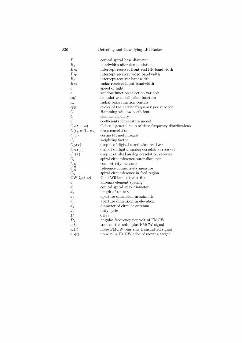
7/17/2019 1596932341 Intercept Radar.pdf
http://slidepdf.com/reader/full/1596932341-intercept-radarpdf 861/891
830 Detecting and Classifying LPI Radar
B conical spiral base diameterBa bandwidth after demodulationBIR intercept receiver front-end RF bandwidthBIV intercept receiver video bandwidthBI intercept receiver bandwidthBRi radar receiver input bandwidthc speed of lightc window function selection variablecdf cumulative distribution functioncn radial basis function centerscpp cycles of the carrier frequency per subcodeC Hamming window coefficientC channel capacity
C coefficients for seastate modelC f (t,ω,φ) Cohen’s general class of time frequency distributionsC (td,α; T r,αr) cross-correlationC (x) cosine Fresnel integralC i weighting factorC D(τ ) output of digital correlation receiverC DA(τ ) output of digital-analog correlation receiverC I (τ ) output of ideal analog correlation receiverC l spiral circumference outer diameterC M connectivity measureC RM reference connectivity measureC u spiral circumference in feed regionCWDx(,ω) Choi-Williams distributiond antenna element spacingd conical spiral apex diameterdγ length of route γ da aperture dimension in azimuthde aperture dimension in elevationda diameter of circular antennadc duty cycleD delayDf angular frequency per volt of FMCWe(t) transmitted noise plus FMCW signalec(t) noise FMCW plus sine transmitted signaleR(t) noise plus FMCW echo of moving target

7/17/2019 1596932341 Intercept Radar.pdf
http://slidepdf.com/reader/full/1596932341-intercept-radarpdf 862/891
List of Symbols 831
E amplitude of noise plus FMCW signalE energyE R amplitude of noise plus FMCW echoERPR eff ective radiated power of radarERPJ eff ective radiated power of jammerERPC eff ective radiated power of data communication nodef 1b upslope beat frequencyf 2b downslope beat frequencyf b beat frequencyf c carrier frequencyf l lower frequency limit of spiral antennaf u upper frequency limit of spiral antennaf u unambiguous Doppler frequency
f clk clock frequencyf (t) continuous signalf dmax random binary phase modulation Doppler tolerancef maxb maximum beat frequency
f HL hard-limiting nonlinearityf l(n),f l (n) kernel function for Wigner-Ville distributionf m video modulation signalf j FSK transmitted frequencyf s(y) sigmoid nonlinearity functionf cr critical frequencyf s sampling frequencyf c1 first frequency of a two-tone signalf c2 second frequency of a two-tone signalf (k1, k2) time-frequency imagef I single sawtooth FMCW signalf 0 frequency constantF (u, v) frequency rectangleF i flux power incident on a target
F chirp rate
F angular frequency increment per sampleF I intercept receiver noise factorF R radar receiver noise factorF (u) array patternF μ,ν γ time dependent flow coefficientF 1, F 2 spiral antenna feed points

7/17/2019 1596932341 Intercept Radar.pdf
http://slidepdf.com/reader/full/1596932341-intercept-radarpdf 863/891
832 Detecting and Classifying LPI Radar
g response of the receiverg Tikhonov’s regularization parameterG antenna gainG filter transfer functionG Gabor time-frequency distributionG(x) antenna taper functionGr antenna receive gain along boresightGt antenna transmit gain along boresightG
t antenna transmit gain in side lobeGI intercept receiver antenna gaingn(τ ) modulation functionh heightha,b(t) single prototype wavelet
h correlation integralh impulse responseh(k1, k2) filter maskh(n) histogram
h(q)lk received signal from scatterer q transmitter l , rcvr k
hF 2layer F2-layer height from Earth’s surfaceht dipole height above groundH number of hidden layers in multilayer perceptronH entropyH (u, v) 2D filter transfer functionH d(u, v) ideal lowpass filter transfer functionH (ω) antialiasing filter transfer function
H 0(z) highpass fi
lterH 1(z) lowpass filteri number of the sample in a given frequencyI inphase termI neural network input nodesI (t,ω) intensity imageI b transmission lossI ( j) measure of information in j th messageI c circulator isolationI Bar Barrick’s transmission lossI R network reach
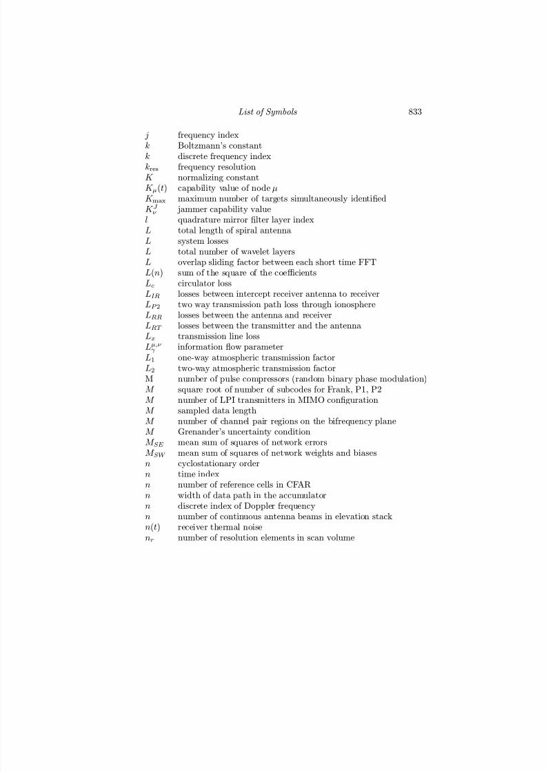
7/17/2019 1596932341 Intercept Radar.pdf
http://slidepdf.com/reader/full/1596932341-intercept-radarpdf 864/891
List of Symbols 833
j frequency indexk Boltzmann’s constantk discrete frequency indexkres frequency resolutionK normalizing constantK μ(t) capability value of node μK max maximum number of targets simultaneously identifiedK J ν jammer capability valuel quadrature mirror filter layer indexL total length of spiral antennaL system lossesL total number of wavelet layersL overlap sliding factor between each short time FFT
L(n) sum of the square of the coefficientsLc circulator lossLIR losses between intercept receiver antenna to receiverLP 2 two way transmission path loss through ionosphereLRR losses between the antenna and receiverLRT losses between the transmitter and the antennaLx transmission line lossLμ,ν γ information flow parameter
L1 one-way atmospheric transmission factorL2 two-way atmospheric transmission factorM number of pulse compressors (random binary phase modulation)M square root of number of subcodes for Frank, P1, P2M number of LPI transmitters in MIMO configurationM sampled data lengthM number of channel pair regions on the bifrequency planeM Grenander’s uncertainty conditionM SE mean sum of squares of network errorsM SW mean sum of squares of network weights and biasesn cyclostationary ordern time indexn number of reference cells in CFARn width of data path in the accumulatorn discrete index of Doppler frequencyn number of continuous antenna beams in elevation stackn(t) receiver thermal noise
nr number of resolution elements in scan volume

7/17/2019 1596932341 Intercept Radar.pdf
http://slidepdf.com/reader/full/1596932341-intercept-radarpdf 865/891
834 Detecting and Classifying LPI Radar
N number of code periods used in correlation receiverN number of arms interleaved within spiral antennaN number of statistically independent noise samplesN FFT sizeN number of receivers in MIMO configurationN total number of discrete samples of timeN discrete short time FFT sizeN c number of subcodes, processing gainN c feature vector dimensionN d number of sections in subdivided scan volumeN e electron densityN m maximum electron densityN p total number of quadrature mirror samples
N r feature vector dimensionN I integration intervalsN B number of Barker phase codesN F number of transmitted continuous frequenciesN F number of tiles displayed in frequencyN I number of noncoherent integration intervalsN RB number of range bins containing clutterN T number of tiles displayed in timeN T total number of phase slots in the FSK/PSK waveformN T number of nodes connected in the networkN P nepersN X beginning target state in Markov chainN Y ending target state in Markov chainN F coherent processing intervalN FFT record lengthN F record lengthN μ total number of nodes connected to node μN μ,ν total number of routes between node μ and ν p(t) aperiodic rectangular window function p(τ ) autocorrelation of the transmitted waveform pj probability of transmitting j th message pr surface wave received power from target pt surface wave radiated power in presence of ground pdf probability density function

7/17/2019 1596932341 Intercept Radar.pdf
http://slidepdf.com/reader/full/1596932341-intercept-radarpdf 866/891
List of Symbols 835
P number of polyphase code periods transmittedP rad radiated power from the antennaP in total input power to the antennaPDD power density at a range RPGR processing gainP avg adaptive average transmitted powerP d probability of detectionP fa probability of false alarmP rerad surface wave power reradiated by targetP t peak power of pulsed emitterP tot total power at receiver using circulatorP N (Z ) square law detector output with no target presentP CW average power of CW transmitter
P RC clutter power within a range binP RT received signal power of the radar from the targetP TR signal power to the intercept receiverPGI intercept receiver processing gainQ quadrature termQ(λμ) knowledge functionr discrete time indexr radial distancerb radial distance to layer’s basere Earth’s radius (6,3781.1 km)rk aperiodic autocorrelation coefficientsrl received signal at antenna l
r1 spiral antenna generating functionR rangeR neural network regularizationR maximum spiral radiusRc code rateRc continuous cross-correlation functionRd range error due to Doppler shiftRfootprint OTHR range along Earth’s surfaceRI range between LPI radar and intercept receiverRI max maximum intercept range for intercept receiverRk target range or path length in kilometersRmax maximum detection range of the LPI radarRcancel,dB reflected power cancelation depth
Ru unambiguous range

7/17/2019 1596932341 Intercept Radar.pdf
http://slidepdf.com/reader/full/1596932341-intercept-radarpdf 867/891
836 Detecting and Classifying LPI Radar
Rx(τ ) time average autocorrelation functionRα
x(τ ) cyclic autocorrelation of a complex time series x(t)R(rtb) periodic autocorrelation functionR(ρ, θ) Radon transformRC range of communication nodeRJ range of jammerRQ network richnessRT target ranges(f ) single sweep FMCW spectrums(f ) roll-off rate single sweep FMCW spectrums(t) complex signalsl(n) orthogonal polyphase complex signals1(t) transmitted signal upslope
s2(t) transmitted signal downslopeS slope of polyphase modulation in time-frequency plotsS (t) complex stationary processS (x) sine Fresnel integralS XN (n, k) estimated timed smoothed periodogramS x(f ) power spectral densityS i,j target scattering coefficient with i, j = V or H
S v(f ) noise plus FMCW correlation output spectrumS x(f ) power spectral densityS αx (f ) spectral correlation densityS αXT W
continuous time-smoothed cyclic periodogram
S γ XN
discrete time-smoothed cyclic periodogram
S d output of up converter MXR1 in noise radarS 1,2 number neurons in first, second hidden layers in MLPSNRIo intercept receiver output SNR from signal processorSNRIi intercept receiver input SNR to signal processorSNRnet SNR for netted radarSNRRi minimum SNR required at the radar inputSNRRo output, Albersheim SNRSNR1 SNR for single monostatic radart timetb subcode period or durationtd round trip propagation time delaytm modulation periodtI smallest radar coherent integration time
t p transmitted frequency duration

7/17/2019 1596932341 Intercept Radar.pdf
http://slidepdf.com/reader/full/1596932341-intercept-radarpdf 868/891
List of Symbols 837
t0 coherent processing intervalt0 signal time of arrivalT code periodT threshold multiplierT f frame timeT h noise radar thresholdT hλ eigenvalue thresholdT int measurement time in noise receiverT p time for target to pass through range cellT A lower limit angle thresholdT B upper limit angle thresholdT N short time FFT windowT N pulse repetition interval
T R delay of RF delay lineT 0 standard temperature in KelvinT W short-time FFT window lengthu(t) periodic complex envelopev, V target velocity∨i eigenvector selectionV t threshold voltageV t maximum closing velocity of the targetw(t) weighting functionwST (f ) frequency domain taper functionwCT (t) time domain cosine-Tukey amplitude taper functionwl(t) additive symmetric zero mean Gaussian noiseW e(f ) power spectrum of transmitted noise plus FMCW signalW n perceptron weighting vectorW x(t,ω), W X(ω, t) Wigner-Ville distributionW (ν ) Fourier transform of windowW N , W M window functions for Choi-Williamsx0 cyclic frequency constantX training matrix for principal components analysisX n n-dimensional perceptron input vectorX q position of scattererX T Fourier transform of x(t)X WF (ω, τ ) windowed Fourier transform of x(t)X r(f ) Fourier transform of the cyclic autocorrelation functionX T W
(t, f ) continuous short time Fourier transform
7/17/2019 1596932341 Intercept Radar.pdf
http://slidepdf.com/reader/full/1596932341-intercept-radarpdf 869/891
838 Detecting and Classifying LPI Radar
X N (n, k) discrete Fourier transformX W (a, b) wavelet transformy1, y2 CFAR noise power levelsym layer semithicknessy pn output of radial basis functionz(t) delay product waveform of x(t)Z square law detector responseZ 0 free space impedance (377 Ω)α cycle frequency (continuous time)αk linear transform of continuous time signal|χ(τ , ν )| ambiguity function magnitude|χNT (τ , ν )| ambiguity function for N reference correlators|χT (τ , ν )| single period ambiguity function
δ sensitivity ratioδ spiral antenna rotation angleδ range diff erence between direct and multipath echoesδ (k) Kroeneker’s delta functionδ F bandwidth incrementδφ phase error from perfect quadratureδ I intercept receiver sensitivityδ R radar receiver sensitivity∆i,j cell value in the diff erence triangle∆α cycle frequency resolution∆ν change in Doppler off set∆f frequency resolution∆t time resolution∆tmin minimum time delay that can be detected∆k points spacing in frequency∆F FMCW modulation bandwidth∆F eff ective modulation bandwidth∆R range resolution∆R eff ective range resolution∆v first blind speed∆w coherent processing interval∆Θ target extent in azimuth∆ω spectral width of the beat frequencyη aperture efficiencyr relative error
γ discrete time cycle frequency

7/17/2019 1596932341 Intercept Radar.pdf
http://slidepdf.com/reader/full/1596932341-intercept-radarpdf 870/891
List of Symbols 839
γ route indexγ noncoherent integration efficiencyγ FMCW flyback factorγ res cycle frequency resolutionγ (t) target reflectivity profileΓ voltage reflection coefficient discrete time index QMFB layer numberλ wavelengthλ information rate of sourceλC 2 decision tempoλd deployment tempoλf fighting tempo
λmin minimum information rateλT characteristic tempoΛOODA maximum operational tempoμ node indexμ local meanμ refractive index of ionosphereν Doppler frequency off setν node indexω radian frequencyωr scan rateωIF intermediate radian frequencyωLO local oscillator angular frequencyΩ frequency boundaryΩa scan coverage in azimuthΩe scan coverage in elevationΩs scan volumeφ(ξ , τ ) kernel function for time-frequency distributionφc phase modulationφi P3, P4 phase sequenceφi incidence angleφi,j Frank, P1, P2 polyphase sequenceφk general phase modulation functionφl orthogonal polyphase sequenceφr phase shiftφ1 FMCW phase

7/17/2019 1596932341 Intercept Radar.pdf
http://slidepdf.com/reader/full/1596932341-intercept-radarpdf 871/891
840 Detecting and Classifying LPI Radar
φT 1 T1(n) polytime sequenceφT 2 T2(n) polytime sequenceφT 3 T3(n) polytime sequenceφT 4 T4(n) polytime sequenceφ0 initial angle of spiral antennaΦ(t) basis setφ( p) Euler function of positive p
ψ grazing angle|ψ(τ , ν )| ambiguity function of mismatched receiverΨb solid angle within the half-power beam contourρ spiral antenna generating functionρλ spiral antenna generating function in wavelengthsρejφ complex correlation coefficient
ρ(t) periodic rectangular windowρV voltage standing wave ratioσ spread of radial basis functionσ1 total received power in noise radarσ2 total power in delayed replica in noise radarσ2 white Gaussian noise powerσ0 incremental backscattering coefficient of the seaσ0i mean sea backscatter coefficient for seastate i
σnj elements of radial basis function covariance matrixσmin minimum detectable radar cross sectionσs transmitted noise signal powerσs Shearman’s definition of backscattering cross-sectionσsr power in the noise radar received signalσFS free-space backscattering cross-sectionσT target radar cross sectionτ off set time delayτ d dwell timeτ R pulse widthτ tk, τ rl propagation time delayθa 3 dB beamwidth in azimuthθe 3 dB beamwidth in elevationθn target azimuth angleθs Radon projection angle for maximum intensityθstart beginning of target’s position in azimuthθstop end of target’s position in azimuth
θ0 angle of main lobe peakξ ( p, q ) multichannel time-frequency LPI detectorξ i target reflectivity

7/17/2019 1596932341 Intercept Radar.pdf
http://slidepdf.com/reader/full/1596932341-intercept-radarpdf 872/891
Glossary
AARGM Advanced antiradiation guided missileACF Autocorrelation functionADC Analog-to-digital converterAEA Airborne electronic attackALCM Air launched cruise missileAMRFC Advanced multifunction RF conceptAO Acousto-opticAOA Analysis of alternativesAOA Angle of arrivalAREPS Advanced Refractive Eff ects Prediction SystemARES Aff ordable reactive strike missileARM Antiradiation missileARMIGER Antiradiation missile with intelligent guidance and extended rangeARSR Air route surveillance systemASCM Antiship capable missileATR Automatic target recognitionAWACS Airborne warning and control system
AZ AzimuthB-F BifrequencyBMEWS Ballistic missile early warning systemBPF Bandpass filterBPSK Binary phase shift keyingC2 Command and controlCARA Combined Altitude Radar AltimeterCCD Charge coupled deviceCFAR Constant false alarm rateCMRA Cruise Missile Radar AltimeterCOSPAR Committee of Space ResearchCSIST Chung-Shan Institute of Science and Technology
841

7/17/2019 1596932341 Intercept Radar.pdf
http://slidepdf.com/reader/full/1596932341-intercept-radarpdf 873/891
842 Detecting and Classifying LPI Radar
CW Continuous waveformCWD Choi-Williams distributionDAC Digital-to-analog converter
DARPA Defense Advanced Research Projects AgencyDC Direct currentDDS Direct digital synthesizerDFT Discrete Fourier transformDFSM Direct frequency-smoothing methodDIP Digital information pheromonesDLVA Detector logarithmic video amplifiersDoD Department of DefenseDRFM Digital radio frequency memoryDSP Digital signal processingEA Electronic attackEL ElevationELINT Electronic intelligenceEP Electronic protectionERP Eff ective radiated powerES Electronic supportEW Electronic warfareEWO Electronic warfare officerFAM FFT accumulation methodFET Field eff ect transistorFFT Fast Fourier transformFH Frequency hoppingFIR Finite impulse responseFLAPS Flat parabolic surfaceFLIR Forward looking infrared
FMCW Frequency modulation CWFOT Optimum working frequencyFOV Field of viewFSK Frequency shift keyingGAO General accounting officeGCS Ground control stationGDA Great deluge algorithmGOCFAR Greatest-of constant false alarm rateGPS Global positioning systemGUI Graphical user interface

7/17/2019 1596932341 Intercept Radar.pdf
http://slidepdf.com/reader/full/1596932341-intercept-radarpdf 874/891
Glossary 843
HARD Helicopter and Aircraft/Radar DetectionHARM High-speed antiradiation missileHCI Human computer interface
HDAM HARM destruction of enemy air defense attack moduleHEMT High electron mobility transistorHTS High temperature superconductorHTS HARM targeting systemHPM High power microwaveIADS Integrated air defense systemICAP Increased capabilityIF Intermediate frequencyIFF Identification friend or foeIG Ionosphere indexIIR Imaging infraredIMU Inertial measurement unitINS Inertial navigation systemIR InfraredIRI International Reference IonosphereIRST Infrared search and trackISAR Inverse synthetic aperture radarISL Integrated side lobe levelJCC JORN coordination centerJORN Jindalee over-the-horizon networkJSR Jam-to-signal ratioJSTARS Joint Surveillance and Target Attack Radar SystemLAMPS Light Airborne Multipurpose SystemLAN Local area networkLANTIRN Low-Altitude Navigation and Targeting Infrared for Night
LCM Least common multipleLNA Low noise amplifierLO Local oscillatorLPF Lowpass filterLPI Low probability of interceptLPID Low probability of identificationLPIT Low probability of intercept toolboxLPRF Low pulse repetition frequencyLUT Lookup tableMALD Miniature Air Launched DecoyMALI Miniature Air Launched InterceptorMATLAB Matrix LaboratoryMF Matched filter
7/17/2019 1596932341 Intercept Radar.pdf
http://slidepdf.com/reader/full/1596932341-intercept-radarpdf 875/891
844 Detecting and Classifying LPI Radar
MFAB Marginal frequency adaptive binarizationMIMO Multiple input multiple outputMIP Millions of instructions per second
MLP Multilayer perceptronMMIC Monolithic microwave integrated circuitMMW Millimeter waveMRSR Multirole Survivable RadarMTD Moving target DopplerMTI Moving target indicationMUF Maximum usable frequencyNATO North Atlantic Treaty OrganizationNCW Network centric warfareOLPI Omnidirectional LPI radarOODA Observation-orientation-decision-actionOTH Over-the-horizonOTHR Over the horizon radarPACF Periodic autocorrelation functionPAF Periodic ambiguity functionPAGE Portable air-defense guard equipmentPALS Precision Approach and Landing SystemPANDORA Parallel array for numerous diff erent operational research activitiesPCA Principal components analysisPDW Pulse descriptor wordPG Passive guidancePGM Precision guided munitionsPLL Phase-locked loopPPI Planned position indicatorPRF Pulse repetition frequency
PRI Pulse repetition intervalPSD Power spectral densityPSK Phase shift keyingPSL Peak side lobe levelPWVD Pseudo Wigner-Ville distributionQMF Quadrature mirror filterQMFB Quadrature mirror filter bankRAAF Royal Australian air forceRAM Rolling airframe missileRBF Radial basis functionRBPC Random binary phase codeRCS Radar cross sectionRF Radio frequency

7/17/2019 1596932341 Intercept Radar.pdf
http://slidepdf.com/reader/full/1596932341-intercept-radarpdf 876/891
Glossary 845
RISP Relative to isotropic antenna at same positionRNR Random noise radarRNFR Random noise plus FMCW radar
RNFSR Random noise FMCW plus sine radarRPC Reflected power cancelerRF Radio frequencyRPM Revolutions per minuteRPV Remotely piloted vehiclesRX ReceiverRTIC Real time into the cockpitRTOC Real time out of the cockpitRWR Radar warning receiverSAM Surface-to-air missileSAR Synthetic aperture radarSATCOM Satellite communicationSAW Surface acoustic waveSCD Spectral correlation densitySCR Signal-to-clutter ratioSEAD Suppression of enemy air defenseSEI Specific emitter identificationSFDR Spurious free dynamic rangeSIGINT Signals intelligenceSJR Signal-to-jam ratioSLR Side lobe ratioSNR Signal-to-noise ratioSSBM Single-sideband modulatorSSN Sun spot numberSTAP Space time adaptive processing
STC Sensitivity time controlSTFT Short-time Fourier transformSVD Singular value decompositionTALS Tactical Automatic Landing SystemTCR Target-to-clutter ratioTEL Transporter erector launcherT-F Time-frequencyTJS Tactical Jamming SystemTOA Time of arrivalTR Transmit and receiveUAV Unmanned aerial vehicleUCARS UAV Common Automatic Recovery System

7/17/2019 1596932341 Intercept Radar.pdf
http://slidepdf.com/reader/full/1596932341-intercept-radarpdf 877/891
846 Detecting and Classifying LPI Radar
UHF Ultra high frequencyU.K. United KingdomURSI Union of Radio Science International
U.S. United StatesUSAF United States Air ForceUT Universal timeUTC Coordinated universal timeUWB Ultra widebandVCO Voltage controlled oscillatorVHF Very high frequencyVLSI Very large scale integrated circuitsVSTOL Vertical stationary take-off and landingWGN White Gaussian noiseWRF Waveform repetition frequencyWT Wavelet transformWVD Wigner-Ville distributionWWII World War IIXNOR Exclusive not ORXOR Exclusive OR
7/17/2019 1596932341 Intercept Radar.pdf
http://slidepdf.com/reader/full/1596932341-intercept-radarpdf 878/891
About the Author
Phillip E. Pace is a professor in the department of electrical and computerengineering at the Naval Postgraduate School (NPS). He received B.S. andM.S. degrees from Ohio University in 1983 and 1986, respectively, and a Ph.D.from the University of Cincinnati in 1990 — all in electrical and computer
engineering. Prior to joining NPS, he spent 2 years at General DynamicsCorporation, Air Defense Systems Division, as a design specialist in the RadarSystems Research Engineering Department. Before that, he was a member of the technical staff at Hughes Aircraft Company, Radar Systems Group, for 5years. He was selected for the Outstanding Research Achievement Award in1994, 1995, and 1998 for his work at NPS in electronic warfare, and receivedthe 1995 Association of Old Crows (AOC) Academic Training Award.
Dr. Pace directs the NPS Center for Joint Services Electronic Warfare, hasbeen the chairman of the Navy’s Threat Missile Simulator Validation Work-ing Group since October 1998, and was a participant on the Navy’s NULKABlue Ribbon Panel in January 1999. He is the author of the textbookAdvanced Techniques for Digital Receivers (Artech House, 2000), and has
been a principal investigator on numerous research projects in the areas of receiver design, signal processing, electronic warfare, and weapon systemsanalysis. Dr. Pace invented the concept of symmetrical number systems,has five patents, over thirty journal publications and is a senior memberof the IEEE.
847

7/17/2019 1596932341 Intercept Radar.pdf
http://slidepdf.com/reader/full/1596932341-intercept-radarpdf 879/891

7/17/2019 1596932341 Intercept Radar.pdf
http://slidepdf.com/reader/full/1596932341-intercept-radarpdf 880/891
Index
A
Abdullah, 553Activation function, 630AD1990 altimeter, 45
Adaptive binarization 637—639Agility, 325—326Alarm ARM, 564Altimeter, 41—45
AD1990, 45AHV-2100, 45CARA, 42CMRA, 43GRA-2000, 44HG-9550, 43PA-5429, 44
Ambiguity function, 68Amplitude weighting, 77AMRFC, 13
Amplifierpredetection, 28postdetection, 28
AN/APG-77, 56—57AN/APS-147, 56AN/APQ-181, 56-57Analog processor, 20Analog to digtal converter, 20Anti-ARM, 606—612
AN/TLQ-32 ARM-D decoy, 611Cosmic Shield, 607flaps decoy, 608—609Gazetchik, 610—611VHF/UHF, 607
Patriot, 607position flexibility, 606Swedish GLV200, 607
Swiss Air Guard, 607twinkle transmission, 607warning radar and decoy,
608—609Antiradiation missile (ARM), 4,
AARGM, 569—571, 592—593Alamo, 578—579Alarm, 564, 597—599antenna design, 559—566ARES, 593ARMIGER, 600Corvus, 554dual-mode, 567, 569FT-2000, 604—606HARM, 591—592Harpy, 601—602Kegler, 585—586Kelt, 580—581Kh-27, 585
Kickback, 587Kilter, 584—585Kingfish, 581—582Kitchen, 579—580,Krypton, 565—566, 587—589Kyle, 582—584LPI processing, 572—576Martel, 596—597millimeter, 569—570performance metrics, 577Rolling airframe missile, 594—595seeker, 566—571, 605Shrike, 555, 589—590Sidearm, 593—594
signal processing, 571—572Standard, 591STAR-1, 603—604
849

7/17/2019 1596932341 Intercept Radar.pdf
http://slidepdf.com/reader/full/1596932341-intercept-radarpdf 881/891
850 Detecting and Classifying LPI Radar
summary (Russian), 578targets, 557Tien Chien IIA, 598—599
Antiship missileRBS-15, 58—60seeker technology, 301—305
Antenna, 5aperture distribution, 7bandwidth, 6beamwidth (half-power), 5dimension, 6eff ective area, 25efficiency, 5gain, 5isotropic, 24isolation (using circulator),
96—97
isolation (using RPC), 97—99main lobe, 5nonscanning, 12pattern, 5—10pencil beam, 6, 12phased array, 6—7radiation intensity, 8scan pattern, 10—13side lobe, 5—10side lobe ratio, 5simultaneous transmit, 13spiral design, 559—566stacked beam, 12taper functions, 9
Atmosphericabsorption, 17transmission, 25
Autocorrelation function, 22Autonomous classification
authority, 621—622feature extraction, 634—639multilayer perceptron, 624, 629—
632radial basis function, 624, 632—
633results with MLP, 638—645, 667—
674results with RBF, 642, 646—648,
674—681time-frequency, 620—621
training, 631Sheridan levels, 622-623
Autonommous parameter extraction
Wigner-Ville with Radon, 688—696
AHV-2100 altimeter, 45
B
Back lobe, 5Bandwidth
fractional, 210instantaneous fractional, 211intercept receiver, 28—29modulation (FMCW), 19—20phase code, 127radar, 26
Barker phase codesbinary, 128—133polyphase, 133—139
Basis functions, 468Beamforming
digital, 14Beamwidth, 6Beat frequency, 18, 103—104bifrequency, 513,523—524, 699Blind speed, 102
for OTHR, 264Boltzmann’s constant, 26Bottleneck, 333, 341
C
Capability value, 326—327 jammer, 338
CARA altimeter, 42CHAIN HOME, 553Channel capacity, 334
unifying principal in EW, 334-335
Chinese OTH-B, 272—276Chinese remainder theorem, 267—269Choi-Williams dist.
BPSK analysis, 449, 452—454classification, 634—637comparison to WVD, 446Costas analysis, 458, 461—462

7/17/2019 1596932341 Intercept Radar.pdf
http://slidepdf.com/reader/full/1596932341-intercept-radarpdf 882/891
Index 851
demodulation, 400FMCW analysis, 449—451hybrid analysis, 458, 463
polyphase analysis, 455—457polytime analysis, 455, 458—460
Classification, see Autonomous
classi fi cation
CMRA altimeter, 43Coherent integration, 12Combat losses, 557Communications, 13Compass Call, 556Complete residue, 716—717Compound Barker code, 128—129Compression ratio, 127Conical scan, 13Connectivity measure
extended, 333generalized, 326—328reference, 328—329
Continuous waveform, 16Correlation processor, 21—24
coherence, 22for noise, 238—243Fourier transform,21
Corvus ARM, 554—555Cosmic Shield, 607Costas codes, 191—195Critical frequency, 257Cyclostationary processing
BPSK analysis, 528—531, 532—534Costas analysis, 540, 544cycle frequency, 514cycle frequency resolution, 519cyclic autocorrelation, 514—515cyclic spectral analysis, 515demodulation, 400direct frequency smoothing,
522—525FFT accumulation method,
520—522FMCW analysis, 531, 535—537,
805—807FMCW parameter extraction,
699—704Frank analysis, 809—812Grenander’s uncertainty, 519
noise analysis, 543, 545—546time-domain implementation, 516polyphase analysis, 535, 537,
539—541, 809—820polytime analysis, 540, 542—543,
821—827spectral correlation density,
515—520
D
Database, 638—640Database extended, 660—666Decision speed, 324Decoy, 558—559Demodulation, 400Detection,
homodyne, 18—20maximum range, 26range, 24—26
Detectorenvelope approximation, 84linear 29square-law, 28—29, 395
Diff erence triangle, 191—195Digital RF memory, 396Digital-to-analog converter, 92—93Direct digital synthesizer, 20,
generating linear FM using,91—94,
RPC using, 98—99Direct RF sampling, 398—400Distruction, 558Doppler,
clutter spectrum, 259—261matrix correlation, 23side lobe reduction, 23, 75—78,
110—113zero, 22
Down conversion, 397—398Duty cycle, 14—15Dwell time, 11—13
E
Eagle, 48—49Eff ective radiated power, 18

7/17/2019 1596932341 Intercept Radar.pdf
http://slidepdf.com/reader/full/1596932341-intercept-radarpdf 883/891
852 Detecting and Classifying LPI Radar
Electronic attackFMCW, 115unifying principal, 334—335
joint airborne, 556on information grid, 337—338on netted radar, 352—360
Electronic protection,unifying principal, 334—335
Electronic warfare, 13receivers, 387—388
Electronic warfare officer, 556ELINT, 37Emitter clustering, 687—688Entropy, 333—336Espenschied, Lloyd, 41Extinction coefficient, 25
F
Fan beam, 6Field of view, 10
resolution elements, 10FM interrupted CW (OTHR),
282—287FMCW radar
advantages of, 81—82block diagram, 18—20modulation period, 102—104out-of-band emission, 270—271range-Doppler cross coupling, 102received signal, 100—101waveform design, 86—89, 91—94waveform nonlinearities, 105—106waveform spectrum, 89—91
Fourier transform, 7, 18FFT accumulation method, 520-
522FMCW range profile, 84LPI detection, 576
Frame time, 11—13Frank code
example for PAF 71—75peak side lobe, 75polyphase, 139, 143—148
Frequency hoppingadvantages, 187—189transmitted signal, 189
range resolution, 189—191orthogonal codes, 370—375
FSK — see Frequency hopping
FSK/PSK — see Hybrid techniques
G
Generalization, 630Gibb’s phenomena, 474Global information grid, 320GOCFAR, 84—85, 104GRA-2000 altimeter, 44Grating lobes, 14Growler EA-18G, 556
H
Hamming window, 77, 447Hann window, 77Harr fiter, 472—473HARD, 48—49HG-9550 altimeter, 43Homodyne detection, 18Human computer interface, 621—623Hybird techniques, 195—198
target matched, 199—204
I
Information rate, 334Integration, 18—20
coherent, 28LPI detection, 574—576netted radar, 348—349noncoherent efficiency, 29noncoherent, 19, 20postdetection, 85—86
Intercept receiver, 4challenges, 400—402maximum range, 28
Interrupted CW, 16Ionospheric eff ects (HF), 253—261
J
Jam-to-signal ratiocommunication node, 337—338

7/17/2019 1596932341 Intercept Radar.pdf
http://slidepdf.com/reader/full/1596932341-intercept-radarpdf 884/891
Index 853
radar node, 352—353Jamming, 556, 621JY-17a, 53—55
K
Kh-31 ARMseeker, 565—566
Klipper (bandwidth), 28Knowledge function, 335-336
L
Landing systems, 45—47PALS, 46TALS, 46UCARS, 46
LANTIRN, 58Lethality, 326Look-through, 388—389Low noise amplifier, 84Low probability of detection, 3
definition, 4Low probability of intercept radar,
antenna characteristics, 5—14definition, 3, 31deramping detection of, 576discriminator, 573—574multichannel detection, 574—576netted, 342origin of, 29transmitter characteristics,
14—18requirement, 4sensitivity definition, 30—31summary of characteristics, 18
Lowpass filtering, 648—651Lookup table, 92LPI toolbox (LPIT), 709—711LPIsimNet,
information network, 338—345radar network, 353—360tutorial, 721—739
M
Main lobe, 5
MALD, 558—559MALI, 59Maneuverabilty,, 323—324Markov chain, 85Marginal frequency, 634—638, 651—656Matched filter 22Maximum usable frequency, 257MIMO, 349—352Missile systems, 58—62MMIC, 116Modified feature extraction, 648—660Modified sinc filter, 473—474Modulation, 16
bandwidth (FMCW), 20
period (FMCW), 20, 102—104triangular,, 86—91LPI, 36—37
Moving target indication, 107—108MRSR, 55Multifunction aperture, 13Multilayer perceptron, 629—632
generalization, 630
N
Narayanan noise radar, 215—219PAF, PACF, 219—222
Netted LPI radar, 342-345advantages, 346—347LIPsimNet analysis, 353—360MIMO, 349—352orthogonal codes, 362—372signal-to-noise ratio, 348—349signal model, 349—352use of noise in, 374, 376—377
Network centric warfareblock diagram, 321definition, 320entropy, 333-336global information grid, 320information rate, 334 jam-to-signal ratio, 337—338LPIsimNet, 338—345metrics 326—337

7/17/2019 1596932341 Intercept Radar.pdf
http://slidepdf.com/reader/full/1596932341-intercept-radarpdf 885/891
854 Detecting and Classifying LPI Radar
network reach, 329—331network richness, 333-336receivers, 389—391
requirements, 322sensor grid, 321shooter grid, 322
Network reach, 329—331, 336Network richness, 333-336Noise radar
correlation receivers, 238—243MALI, 59millimeter wave, 238Narayanan design, 215—222netted radar, 374, 376—377principles, 212—215random noise FMCW plus sine,
227, 229—234
random noise plus FMCW,222—227
ultrawideband, 210—212
O
OLPI, 13, 179—182OODA, 324—325, 326Operational tempo, 324
maximum, 336—337Origin of LPI, 29Orthogonal waveforms, 358, 361—362
frequency hopping, 370—375MIMO, 350—352OTHR, 377—378polyphase codes, 362—370
OTHR systemsDoppler spectrum, 259—261ionosphere, 253—261netted configurations, 377—378sky wave, 252—280sky wave waveforms, 265—271surface wave, 276, 281—294surface wave waveforms, 282—288
OTHR waveforms, 249—251
P
P1 code, 148—151P2 code, 152—155
P3 code, 152, 156—157P4 code, 157, 160—162PA-5429 altimeter, 44
PAGE, 51—52PALS landing system, 46PANDORA, 113—114Patriot, 607Peak power, 14Perceptron
single, 625—628Perfect codes, 128
PACF, 69, 74—75Periodic ambiguity, 67—78
definition, 69generating results, 713—714periodicity, 70
Periodic autocorrelation, 67—78
definition, 68—69Pencil beam, 6Phased array, 6—7, 12Phase code, 21
advantages, 125—126binary, 128—133period, 127rate, 127range resolution, 127transmitted signal, 126—127
Pilot radar, 31—36technical characteristics, 33sensitivity, 34
Platform centric, 319—320Pointer, 50—51Polarization, 6Polyphase codes, 134—162
Barker, 134—142Frank, 139, 143—148orthogonal, 362—372P1, 148—151P2, 152—155P3, 152, 156—157P4, 157, 160—162
Polytime codes, 163—178T1(n), 163—165T2(n), 165, 168—171T3(n), 169, 172—174T4(n), 169, 175—178
Position flexibility, 606

7/17/2019 1596932341 Intercept Radar.pdf
http://slidepdf.com/reader/full/1596932341-intercept-radarpdf 886/891
Index 855
Powerattenuation coefficient, 25average, 15
density, 24—25peak, 15received, 25
Power management, 16—18in seeker, 17using constant SNR, 310—312
Prime number, 715Primitive roots, 717—719Principal components analysis, 648,
656—660Probability of detection, 19Probability of false alarm, 19Processing gain, 19
FMCW, 20
intercept receiver, 28—29phase code, 20random binary phase modulation,
211PSK — see polyphase codePulse compression, 15—16, 18—24Pulse descriptor words, 396Pulsed radar, 14
Q
Quadrature mirror filteringBPSK analysis, 489—494, 773—776complex input example, 482—487Costas analysis, 499, 502—503demodulation, 400FMCW analysis, 487—489, 771—
772Frank analysis, 777—780Harr filter, 472—473hybrid analysis, 499, 504—505noise analysis, 499, 506—508polyphase analysis, 494—498, 777—
780, 781—795polytime analysis, 495, 499—501,
797—803polyphase parameter extraction,
695—699short-time Fourier transform, 469tree structure, 476—482
two channel analysis, 474—476wavelet decomposition, 468wavelet filters, 472—474
wavelet transform, 469—471Quiet radar, 30Quiet naval radar CRM-100, 53
R
Radarpulsed conventional, 14, 35, 42warning receiver, 37
Radar cross sectionfree space backscattering, 291low values, 306—307microwave 290Shearman’s definition, 291
Radial basis function, 624, 632—633Euclidean norm, 632Gaussian basis, 633
Radon transform, 689—692Random binary phase, 234—237
PAF, PACF, 236—237
Random noise plus FMCW, 222—227PAF, PACF, 225—228
Random noise FMCW plus sine, 227,229—234
PAF, PACF, 230—234Range
detection, 24—26interception, 27—29maximum detection, 26, 30, 32maximum interception, 27—28, 30resolution, 102
RBS-15, 58—60Receiver (intercept)
challenges with, 400—402sensitivity, 27—28
Receiver (radar)bandwidth, 26comparison, 392—396correlation, 23, 238—243matched, 22, 108—110mismatched, 24, 75—78, 110—113noise factor, 26sensitivity, 25—26
7/17/2019 1596932341 Intercept Radar.pdf
http://slidepdf.com/reader/full/1596932341-intercept-radarpdf 887/891
856 Detecting and Classifying LPI Radar
Reduced residue, 716—717Reflected power canceler, 83Reference signal, 21—24
Regularization, 630—631Tikhonov’s parameter, 631
Resolutioncycle frequency, 519FMCW range, 102sky wave OTHR, 264phase code range, 127velocity, 102
S
Samples per subcode, 73Scan pattern, 11-13
confusion, 13
raster scan, 11Sea clutter, 308—310Sea state, 308Search mode processing
FMCW, 101—105Seekers
airborne, 58—61torpedo, 61—62
Sensitivitycomparison, 29intercept receiver, 27—28Pilot’s, 35radar, 25—26receiver comparison, 395—396
Sensor grid, 321Sheridan levels, 622—623Short-time Fourier transform, 469
in cyclic spectrum estimation,518—519
Side lobes, 5—10ACF, PACF, PAF, 70—71definitions of peak, 70—71OTHR 265—266
Side lobe ratio, 5Taylor, 9—10
Sigmoid, 625—626, 630Signal-to-noise ratio,
Albersheim relation, 19input required (radar), 26for netted radar, 348—349
output (radar), 26Pilot’s required, 35processing gain, 19
time-bandwidth, related to 19Sinc filter, 473—474Single sideband modulator, 92—94Situational awareness, 323Sky wave OTHR, 249—251
critical frequency, 257detection range, 271—276distance coverage 259footprint, 274—276Doppler clutter, 259—261ionosphere eff ects, 253—259JORN, 261—263LPI considerations, 265—271maximum usable frequency, 257
waveform repetition frequency,266—269
SMART-L, 11Spearfish, 61Spiral antenna, 559—566
Archimedean, 563—564equiangular, 560—562logarithmic, 559conical, 559—560conical equiangular, 564—565
STC, 82Subcode, 20
number of, 20period, 20—22
Superconductor, 118—119Suppression
beginnings, 553definitions, 552—553Eagle example, 331-333enemy integrated air defense,
551—553look-through, 388—389
Surface wave OTHR, 249—251, 276,278, 281
detection range, 288—294LPI considerations, 282—288SWR 503, 281—283
Surveillance systemsairborne 56—58ground based, 48—55
7/17/2019 1596932341 Intercept Radar.pdf
http://slidepdf.com/reader/full/1596932341-intercept-radarpdf 888/891
Index 857
Swarm, 391—392Swedish GLV200, 607Swiss Air Guard, 607
T
TALS landing system, 46Taper, 7—9, 12Tapped delay line, 22—24Target-to-clutter ratio, 312—315Taylor distribution, 8—10, 12Temperature, 26Time-bandwidth,
FMCW, 19Time-frequency processing
Choi-Williams distribution,445—463
Gabor distribution, 574—576quadrature mirror filtering,
467—509Wigner-Ville distribution,
405—442Time-on-target, 11—13Time smoothing, 520—522Track mode processing
FMCW, 104—105Training, 631Transmission line, 95—96Transmit,
multiple simultaneous, 13peak power, 14power management, 16
Transmittercontinuous waveform, 15solid state, 15
Twinkle transmission, 607
U
UCARS landing system, 46Ultra-low (side lobes), 8Uniform window, 77Unmanned aerial vehicle, 391—392,
595—596
V
Variant, 52—53
Vietnam, 555—556
W
Wavelet filters, 472—474Wavelet transform, 469—471Weighting
Hamming window, 77, 104Hann window, 77
Welsh construction (Costas), 193—195Wiener filter, 692—Wigner-Ville dist. (WVD), 405—442
BPSK analysis, 421—426comparing polyphase results,
431—433complex input example, 411—414continuous 1-D, 406discrete WVD, 407demodulation, 400FMCW analysis, 419—421,
741—743Frank analysis, 745—747FSK, FSK/PSK results, 438—441kernel generation, 408operator (ELINT), 442polyphase analysis, 426—428,
745—747, 749—758polyphase parameter extraction,
688—695polytime analysis, 429—437,
759—769pseudo WVD, 407real input example, 409—411two-tone input example, 414—418
Wild Weasel, 555, 573, 597
Y
YGBSM, 551

7/17/2019 1596932341 Intercept Radar.pdf
http://slidepdf.com/reader/full/1596932341-intercept-radarpdf 889/891

7/17/2019 1596932341 Intercept Radar.pdf
http://slidepdf.com/reader/full/1596932341-intercept-radarpdf 890/891
Recent Titles in the Artech House
Radar Series
David K. Barton, Series Editor
Adaptive Antennas and Phased Arrays for Radar and Communications, Alan J. Fenn
Advanced Techniques for Digital Receivers, Phillip E. Pace
Advances in Direction-of-Arrival Estimation, Sathish Chandran,editor
Airborne Pulsed Doppler Radar, Second Edition, Guy V. Morris andLinda Harkness, editors
Bayesian Multiple Target Tracking, Lawrence D. Stone,Carl A. Barlow, and Thomas L. Corwin
Beyond the Kalman Filter: Particle Filters for Tracking Applications,
Branko Ristic, Sanjeev Arulampalam, and Neil Gordon
Computer Simulation of Aerial Target Radar Scattering,Recognition, Detection, and Tracking, Yakov D. Shirman, editor
Design and Analysis of Modern Tracking Systems, Samuel Blackmanand Robert Popoli
Detecting and Classifying Low Probability of Intercept Radar, Second Edition, Phillip E. Pace
Digital Techniques for Wideband Receivers, Second Edition,James Tsui
Electronic Intelligence: The Analysis of Radar Signals, Second Edition, Richard G. Wiley
Electronic Warfare in the Information Age, D. Curtis Schleher
ELINT: The Interception and Analysis of Radar Signals,Richard G. Wiley
EW 101: A First Course in Electronic Warfare, David Adamy
EW 102: A Second Course in Electronic Warfare, David L. Adamy
7/17/2019 1596932341 Intercept Radar.pdf
http://slidepdf.com/reader/full/1596932341-intercept-radarpdf 891/891
EW 103: Tactical Battlefield Communications Electronic Warfare,David Adamy
Fourier Transforms in Radar and Signal Processing,David Brandwood
Fundamentals of Electronic Warfare, Sergei A. Vakin, Lev N. Shustov,