15325000701603892 powersys

7/29/2019 15325000701603892 powersys

http://slidepdf.com/reader/full/15325000701603892-powersys 1/17

This article was downloaded by: [Van Pelt and Opie Library]On: 10 September 2013, At: 22:57Publisher: Taylor & FrancisInforma Ltd Registered in England and Wales Registered Number: 1072954 Registered office: Mortimer House37-41 Mortimer Street, London W1T 3JH, UK

Electric Power Components and SystemsPublication details, including instructions for authors and subscription information:

http://www.tandfonline.com/loi/uemp20

Solution of Different Types of Economic Load Dispatch

Problems Using a Pattern Search MethodJ. S. Al-Sumait

a, J. K. Sykulski

a& A. K. Al-Othman

b

aElectrical Power Engineering Group, University of Southampton, Highfield, Southampton

United Kingdomb

Electrical Engineering Department, College of Technological Studies, Alrawda, Kuwait

Published online: 21 Feb 2008.

To cite this article: J. S. Al-Sumait , J. K. Sykulski & A. K. Al-Othman (2008) Solution of Different Types of Economic

Load Dispatch Problems Using a Pattern Search Method, Electric Power Components and Systems, 36:3, 250-265, DOI:10.1080/15325000701603892

To link to this article: http://dx.doi.org/10.1080/15325000701603892

PLEASE SCROLL DOWN FOR ARTICLE

Taylor & Francis makes every effort to ensure the accuracy of all the information (the “Content”) containedin the publications on our platform. However, Taylor & Francis, our agents, and our licensors make norepresentations or warranties whatsoever as to the accuracy, completeness, or suitability for any purpose of tContent. Any opinions and views expressed in this publication are the opinions and views of the authors, and

are not the views of or endorsed by Taylor & Francis. The accuracy of the Content should not be relied upon ashould be independently verified with primary sources of information. Taylor and Francis shall not be liable forany losses, actions, claims, proceedings, demands, costs, expenses, damages, and other liabilities whatsoeveor howsoever caused arising directly or indirectly in connection with, in relation to or arising out of the use of the Content.

This article may be used for research, teaching, and private study purposes. Any substantial or systematicreproduction, redistribution, reselling, loan, sub-licensing, systematic supply, or distribution in anyform to anyone is expressly forbidden. Terms & Conditions of access and use can be found at http://www.tandfonline.com/page/terms-and-conditions

http://dx.doi.org/10.1080/15325000701603892

http://www.tandfonline.com/action/showCitFormats?doi=10.1080/15325000701603892

http://www.tandfonline.com/page/terms-and-conditions

http://www.tandfonline.com/page/terms-and-conditions

http://dx.doi.org/10.1080/15325000701603892

http://www.tandfonline.com/action/showCitFormats?doi=10.1080/15325000701603892

http://www.tandfonline.com/loi/uemp20

7/29/2019 15325000701603892 powersys


Electric Power Components and Systems, 36:250–265, 2008

Copyright © Taylor & Francis Group, LLC

ISSN: 1532-5008 print/1532-5016 online

DOI: 10.1080/15325000701603892

Solution of Different Types of Economic LoadDispatch Problems Using a Pattern Search Method

J. S. AL-SUMAIT,1 J. K. SYKULSKI,1 andA. K. AL-OTHMAN2

1Electrical Power Engineering Group, University of Southampton,

Highfield Southampton, United Kingdom2Electrical Engineering Department, College of Technological Studies,

Alrawda, Kuwait

Abstract Direct search (DS) methods are evolutionary algorithms used to solveconstrained optimization problems. DS methods do not require information about thegradient of the objective function when searching for an optimum solution. One such

method is a pattern search (PS) algorithm. This study presents a new approach based on a constrained PS algorithm to solve various types of power system economic load dispatch (ELD) problems. These problems include economic dispatch with valve point (EDVP) effects, multi-area economic load dispatch (MAED), companied economic-environmental dispatch (CEED), and cubic cost function economic dispatch (QCFED).For illustrative purposes, the proposed PS technique has been applied to each of the above dispatch problems to validate its effectiveness. Furthermore, convergencecharacteristics and robustness of the proposed method has been assessed and inves-

tigated through comparison with results reported in literature. The outcome is veryencouraging and suggests that PS methods may be very efficient when solving power system ELD problems.

Keywords ELD, DS method, PS method, evolutionary algorithms, optimization

1. Introduction

Scarcity of energy resources, increasing power generation costs, and ever-growing de-

mand for electric energy necessitates optimal economic dispatch (ED) in today’s power

systems. The main objective of ED is to reduce the total power generation cost while

satisfying various equality and inequality constraints. Traditionally, in ED problems, the

cost function for generating units has been approximated as a quadratic function.A variety of optimization techniques has been applied in solving ELD problems.

Some of these techniques are based on classical optimization formulations, while others

are based on artificial intelligence methods or heuristic algorithms. Many references

present the application of classical optimization methods, such as linear or quadratic

programming, to solve ELD problems [1, 2]. Classical optimization methods are reportedto be highly sensitive to the selection of the starting points and sometimes converge to a

Received 12 October 2006; accepted 13 July 2007.Address correspondence to Dr. Abdrulrahman Al-Othman, Electrical Engineering Department,

College of Technological Studies, P.O. Box 33198, Alrawda, 73452, Kuwait. E-mail: [email protected]

250

7/29/2019 15325000701603892 powersys


Solution of Different Types of Economic Load Dispatch 251

local optimum or diverge altogether. Linear programming methods are fast and reliable,

but have disadvantages associated with the piecewise linear cost approximation. Non-linear programming methods are known to have problems of convergence and algorithmic

complexity. Newton-based algorithms struggle with handling a large number of inequality

constraints [3]. Methods based on artificial intelligence techniques, such as artificialneural networks, are also presented [4, 5]. Heuristic search techniques, such as particle

swarm optimization [3] and genetic algorithms [6], have also been successfully appliedto ELD problems. Finally, hybrid methods have been developed, where the conventional

Lagrangian relaxation approach, a first-order gradient method, and multi-pass dynamic

programming (DP) are combined in [7].

Recently, a particular family of global optimization methods, originally introduced

and developed by researchers in the 1960s [8], has attracted special attention. Known

as DS methods, they are simply designed to explore a set of points around the currentposition, looking for a location that has a better objective value than the existing one.

This family includes PS algorithms, simplex methods (different from the simplex used

in linear programming), Powell optimization, and others [9].

DS methods, in contrast to more standard optimization methods, are often called

derivative-free as they do not require information about the gradient or higher derivativesof the objective function to search for an optimal solution. Thus, DS methods are a popular

choice to solve non-continuous, non-differentiable, and multimodal (i.e., multiple local

optima), optimization problems. Since the ED is one such problem, the proposed method

appears to be a good candidate to achieve efficient solutions [10].

The main objective of this study is to introduce the use of a PS optimization techniquein application to the power system ELD. The performance, effectiveness, and robustness

of the proposed method are assessed via intensive testing and comparison with results

reported in literature. The article is organized as follows: Section 2 introduces the problem

formulation, Section 3 presents a description of the proposed PS algorithm, analysis and

test results are presented in Section 4, followed by concluding remarks.

2. Problem Formulation

Generally, depending on the type of the ELD considered, the traditional formulation is

basically a minimization of summation of the fuel costs of the individual dispatchablegenerators, subject to the real power balanced with the total load demand as well as with

the limits on generators’ outputs. The mathematical form of each type of ED problem

considered in this study may be described as in the following subsections.

2.1. Mathematical Form of EDVP

The inclusion of the valve-point effects is advantageous and makes the modeling of the

fuel-cost function more realistic [11–13]. However, the valve-point effects, which appear

as a sinusoidal term added to the fuel-cost functions, introduce ripples to the heat-ratecurve, and, therefore, create more local minima in the search space.

The objective function of an EDVP is to minimize F , where F is given by

F D

N XiD1

F i .P i /: (1)

7/29/2019 15325000701603892 powersys


252 J. S. Al-Sumait et al.

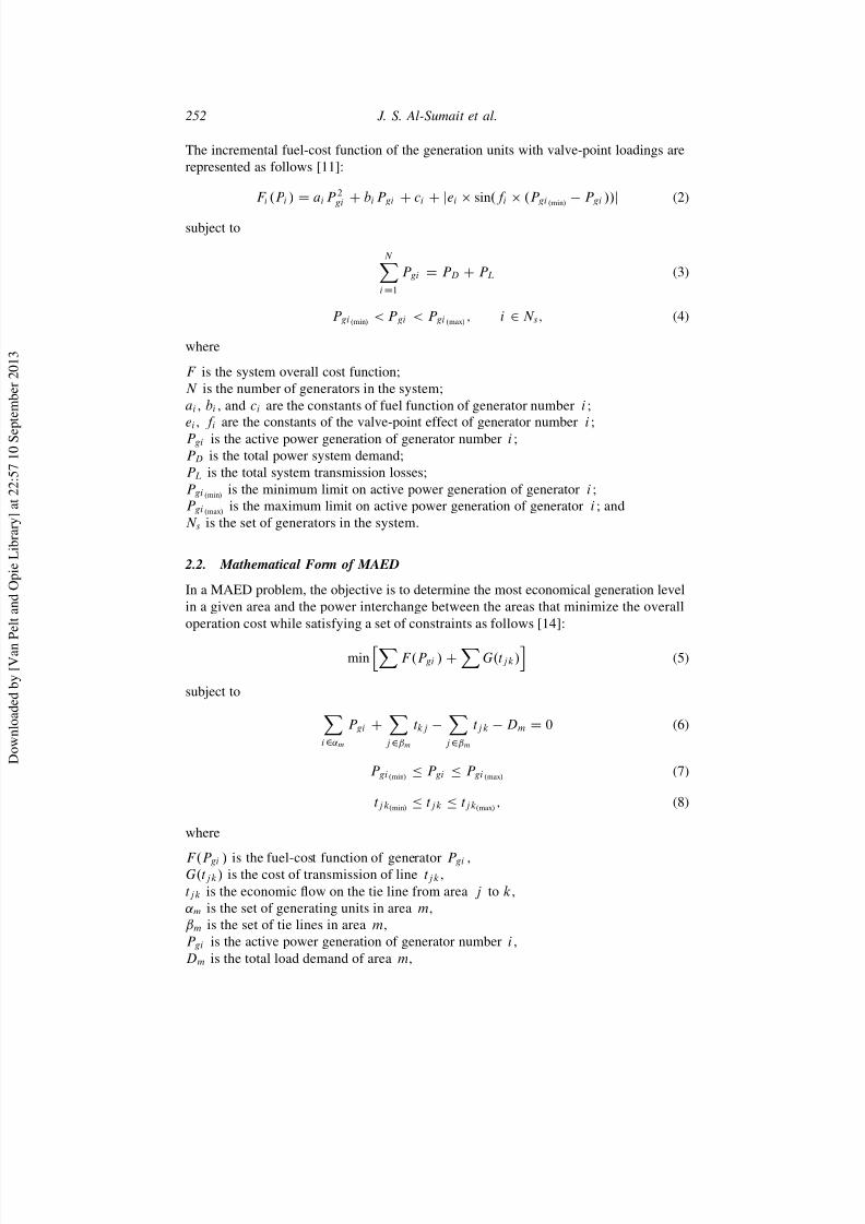
The incremental fuel-cost function of the generation units with valve-point loadings are

represented as follows [11]:

F i .P i / D aiP 2gi C biP gi C ci C jei sin.f i .P gi .min/ P gi //j (2)

subject to

N XiD1

P gi D P D C P L (3)

P gi.min/ < P gi < P gi .max/ ; i 2 N s; (4)

where

F is the system overall cost function;

N is the number of generators in the system;

ai , bi , and ci are the constants of fuel function of generator number i ;

ei , f i are the constants of the valve-point effect of generator number i ;P gi is the active power generation of generator number i ;

P D is the total power system demand;

P L is the total system transmission losses;

P gi .min/ is the minimum limit on active power generation of generator i ;P gi .max/ is the maximum limit on active power generation of generator i ; and

N s is the set of generators in the system.

2.2. Mathematical Form of MAED

In a MAED problem, the objective is to determine the most economical generation level

in a given area and the power interchange between the areas that minimize the overall

operation cost while satisfying a set of constraints as follows [14]:

minhX

F .P gi / CX

G.tjk/i

(5)

subject to

Xi2˛m

P gi CXj2ˇm

tkj Xj2ˇm

tjk Dm D 0 (6)

P gi.min/Ä P gi Ä P gi .max/ (7)

tjk.min/Ä tjk Ä tjk.max/

; (8)

where

F .P gi / is the fuel-cost function of generator P gi ,G.tjk/ is the cost of transmission of line tjk ,

tjk is the economic flow on the tie line from area j to k,

˛m is the set of generating units in area m,ˇm is the set of tie lines in area m,

P gi is the active power generation of generator number i ,

Dm is the total load demand of area m,

7/29/2019 15325000701603892 powersys



P L is the total system transmission losses,

P gi.min/is the minimum limit on active power generation of generator i ,

P gi.max/ is the maximum limit on active power generation of generator i ,

tjk.min/is the minimum limit on active power generation of generator i , and

tjk.max/ is the maximum limit on active power generation of generator i .

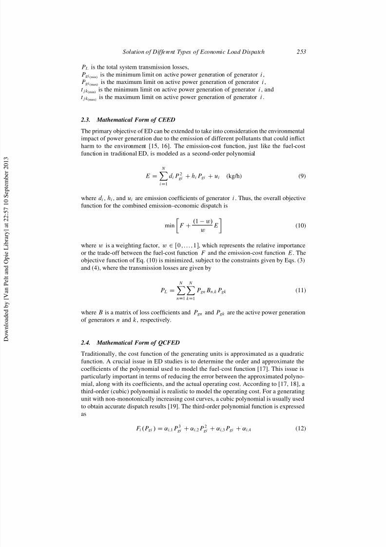
2.3. Mathematical Form of CEED

The primary objective of ED can be extended to take into consideration the environmentalimpact of power generation due to the emission of different pollutants that could inflict

harm to the environment [15, 16]. The emission-cost function, just like the fuel-cost

function in traditional ED, is modeled as a second-order polynomial

E D

N XiD1

d iP 2gi C hiP gi C ui (kg/h) (9)

where d i , hi , and ui are emission coefficients of generator i . Thus, the overall objective

function for the combined emission–economic dispatch is

min

ÄF C

.1 w/

wE

(10)

where w is a weighting factor, w 2 Œ 0 ; : : : ; 1 , which represents the relative importance

or the trade-off between the fuel-cost function F and the emission-cost function E. Theobjective function of Eq. (10) is minimized, subject to the constraints given by Eqs. (3)

and (4), where the transmission losses are given by

P L D

N XnD1

N XkD1

P gnBn;kP gk (11)

where B is a matrix of loss coefficients and P gn and P gk are the active power generation

of generators n and k, respectively.

2.4. Mathematical Form of QCFED

Traditionally, the cost function of the generating units is approximated as a quadratic

function. A crucial issue in ED studies is to determine the order and approximate the

coefficients of the polynomial used to model the fuel-cost function [17]. This issue is

particularly important in terms of reducing the error between the approximated polyno-

mial, along with its coefficients, and the actual operating cost. According to [17, 18], athird-order (cubic) polynomial is realistic to model the operating cost. For a generating

unit with non-monotonically increasing cost curves, a cubic polynomial is usually used

to obtain accurate dispatch results [19]. The third-order polynomial function is expressed

as

F i .P gi / D ˛i;1P 3gi C ˛i;2P 2gi C ˛i;3P gi C ˛i;4 (12)

7/29/2019 15325000701603892 powersys



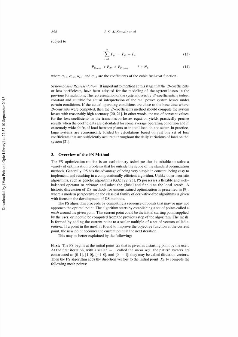
subject to

N

XiD1

P gi D P D C P L (13)

P gi.min/< P gi < P gi .max/

; i 2 N s; (14)

where ˛i;1 , ˛i;2 , ˛i;3, and ˛i;4 are the coefficients of the cubic fuel-cost function.

System Losses Representation. It important to mention at this stage that the B-coefficients,

or loss coefficients, have been adopted for the modeling of the system losses in the

previous formulations. The representation of the system losses by B-coefficients is indeed

constant and suitable for actual interpretation of the real power system losses under

certain conditions. If the actual operating conditions are close to the base case whereB-constants were computed, then the B-coefficients method should compute the system

losses with reasonably high accuracy [20, 21]. In other words, the use of constant values

for the loss coefficients in the transmission losses equation yields practically preciseresults when the coefficients are calculated for some average operating condition and if

extremely wide shifts of load between plants or in total load do not occur. In practice,large systems are economically loaded by calculations based on just one set of loss

coefficients that are sufficiently accurate throughout the daily variations of load on the

system [21].

3. Overview of the PS Method

The PS optimization routine is an evolutionary technique that is suitable to solve a

variety of optimization problems that lie outside the scope of the standard optimization

methods. Generally, PS has the advantage of being very simple in concept, being easy to

implement, and resulting in a computationally efficient algorithm. Unlike other heuristicalgorithms, such as genetic algorithms (GA) [22, 23], PS possesses a flexible and well-

balanced operator to enhance and adapt the global and fine tune the local search. Ahistoric discussion of DS methods for unconstrained optimization is presented in [9],

where a modern perspective on the classical family of derivative-free algorithms is given

with focus on the development of DS methods.

The PS algorithm proceeds by computing a sequence of points that may or may not

approach the optimal point. The algorithm starts by establishing a set of points called amesh around the given point. This current point could be the initial starting point supplied

by the user, or it could be computed from the previous step of the algorithm. The mesh

is formed by adding the current point to a scalar multiple of a set of vectors called a

pattern. If a point in the mesh is found to improve the objective function at the current

point, the new point becomes the current point at the next iteration.

This may be better explained by the following:

First: The PS begins at the initial point X 0 that is given as a starting point by the user.

At the first iteration, with a scalar D 1 called the mesh size, the pattern vectors areconstructed as Œ0 1, Œ1 0, Œ1 0, and Œ0 1; they may be called direction vectors.

Then the PS algorithm adds the direction vectors to the initial point X 0 to compute the

following mesh points:

7/29/2019 15325000701603892 powersys



X 0 C Œ1 0I X 0 C Œ0 1

X 0 C Œ1 0I X 0 C Œ0 1

Figure 1 illustrates the formation of the mesh and pattern vectors. The algorithm computesthe objective function at the mesh points in the order shown.

The algorithm polls the mesh points by computing their objective function values

until it finds one whose value is smaller than the objective function value of X 0. If

there is such a point, then the poll is successful and the algorithm sets this point equal

to X 1.After a successful poll, the algorithm steps to iteration 2 and multiplies the current

mesh size by 2. (This is called the expansion factor and has a default value of 2.)

The mesh at iteration 2 contains the following points: 2 Œ1 0 C X 1, 2 Œ0 1 C X 1,

2 Œ1 0CX 1, and 2 Œ0 1CX 1 . The algorithm polls the mesh points until it finds

one whose value is smaller the objective function value of X 1. The first such point it

finds is called X 2, and the poll is successful. Because the poll is successful, the algorithmmultiplies the current mesh size by 2 to get a mesh size of 4 at the third iteration because

the expansion factor D 2.

Second: If in iteration 3 (mesh sizeD 4) none of the mesh points have a smaller objective

function value than the value at X 2, the poll is declared unsuccessful. In this case the

algorithm does not change the current point at the next iteration, which is X 3 D X 2. Atthe next iteration, the algorithm multiplies the current mesh size by 0.5, a contraction

factor , so that the mesh size at the next iteration is smaller. The algorithm then polls

with a smaller mesh size.

The PS optimization algorithm will repeat the illustrated steps until it finds the

optimal solution for the minimization of the objective function. The algorithm stopswhen any of the following conditions occurs:

the mesh size is less than mesh tolerance, the number of iterations performed by the algorithm reaches a predefined maxi-

mum,

Figure 1. PS mesh points and the pattern.

7/29/2019 15325000701603892 powersys



the total number of objective function evaluations performed by the algorithm

reaches a predefined maximum, the distance between the point found at one successful poll and the point found

at the next successful poll is less than a predefined tolerance, or

the change in the objective function from one successful poll to the next successfulpoll is less than a predefined function tolerance.

Constraint Handling

Many ideas were suggested to insure that the solution will satisfy the constraints [24].

Currently, the only minor weakness in the nonlinear constraints handling procedure

is due to the lack of specific information related to first-order derivatives. Although

many systematic approaches have been employed to handle the nonlinear constraints, the

augmented Lagrangian approach, which has been utilized by PS method, has overcomesuch shortcomings in dealing with nonlinear constraints. Lewis and Torczon [25] stated

that, despite the absence of an explicit estimation of any derivatives (a characteristic of PS

methods), PS-augmented Lagrangian approach exhibits all of the first-order convergenceproperties of the original algorithm advocated by Conn, Gould, and Toint [26, 27]. Lewis

and Torczon [25] were able to overcome such drawbacks by proceeding with successive,inexact minimization of the augmented Lagrangian via PS methods, even without knowing

exactly how inexact the minimization is. As a result, the size of the problem will increase

by introducing new parameters.

The augmented Lagrangian pattern search (ALPS) has been used to solve nonlinear

constraint problems in PS algorithm. ALPS proceeds to solve a nonlinear optimization

problem with nonlinear constraints, linear constraints, and bounds [25, 28–30]. Thevariables bounds and linear constraints are handled separately from nonlinear constraints,

in which a sub-problem is constructed and solved (having the objective function and

nonlinear constraint function) using the Lagrangian and the penalty factors. Such a sub-

problem is minimized using a PS method, where the linear constraints and bounds are

satisfied. ALPS starts with an initial value for the penalty parameter, where the PSalgorithm minimizes a series of the subproblem, which estimates the original problem. If

the required accuracy and feasibility conditions are met, then the Lagrangian estimates

are updated. If not, a penalty factor is added to the penalty parameter. This, in turns,

leads to a new formation of a subproblem and ultimately results in a new minimization

problem. The above steps are repeated until one of the stopping criteria is reached. Forfurther explanation on how PS handles constraints, refer to [25–27, 31].

4. Numerical Results

A set of Matlab files, incorporated in the GA and DS toolbox, implementing the proposedPS method, have been used to solve various ED problems. Thus, cost coefficients of the

fuel cost and the combined objective function for all test cases have been coded in Matlabenvironment.

Initially, several runs have been carried out with different values of the key parameters

of PS, such as the initial mesh size and the mesh expansion and contraction factors. Inthis study, the mesh size and the mesh expansion and contraction factors are selected as

1, 2, and 0.5, respectively. In addition, a vector of initial points, i.e., X 0, was randomly

generated (each initial point is bounded within the generators limits) to provide an initial

7/29/2019 15325000701603892 powersys



guess for the PS to proceed. As for the stopping criteria, all tolerances were set to 106,

and the maximum number of iterations and function evaluations set to 1000.

Case I: EDVP

This test case consists of 13 generating units with a quadratic cost function combined

with the effects of valve-point loading. The unit’s data (upper and lower bounds) along

with the cost coefficients for the fuel cost (a, b, c, e, and f ) for the 13 generators with

valve-point loading are given in [32, 33]. Note that losses are ignored in this case.The PS algorithm has been executed 50 times with different starting points to study

its performance and effectiveness. The solution of the PS method and the execution times

for the 50 runs were compared with the outcome of other evolutionary methods applied

to the same test system as reported in [33]. This numerical experiment compares the

performance of the PS with the other methods in terms of the dispatching costs andconvergence speed. Table 1 shows the optimal solutions determined by PS for the 13

generators, while the execution time and cost comparison are shown in Table 2.

As can be seen from Table 2, the optimum solution of the PS is better than the solu-tions of all the other evolutionary methods. Moreover, the execution time is significantly

shorter than for the other methods [33].

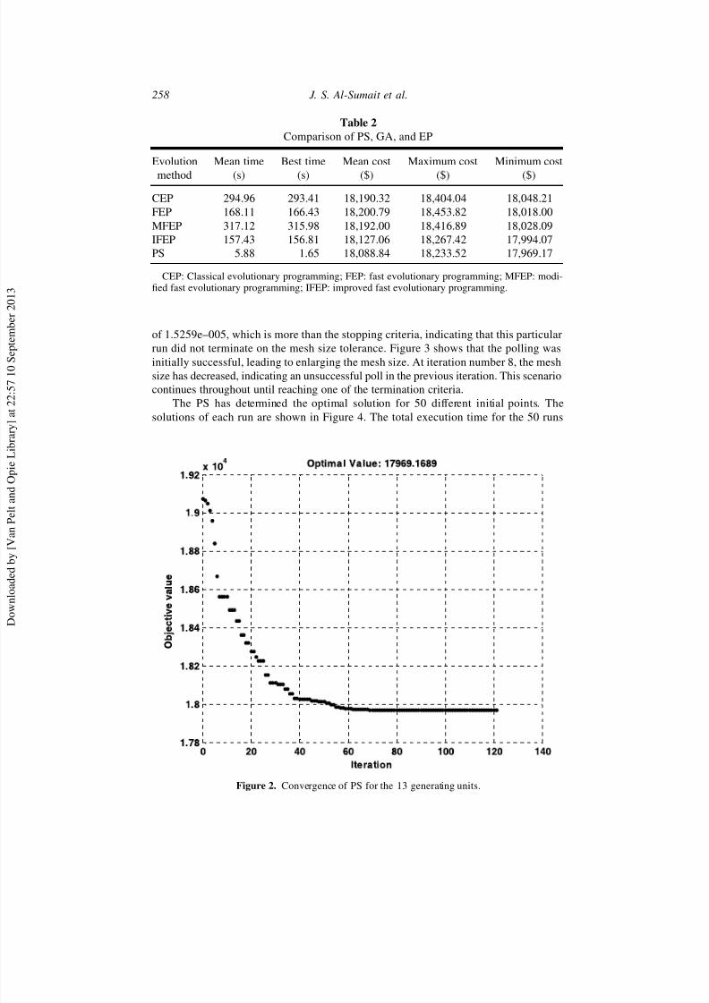
The convergence of the PS process is shown in Figure 2, where only 70 iterationswere needed to locate the optimal solution. However, PS may be allowed to continue

the search in the neighborhood of the optimal solution to increase the confidence in the

result. In this case, the PS terminates after 52 further iterations (a total of 122).

Figure 3 illustrates the mesh size throughout the convergence process. It is apparent

that the mesh size decreases until the algorithm terminates, in this case at a mesh size

Table 1

Generator loading and fuel cost determined byPS with total load demand of 1800 MW

Generator

Generator production

(MW)

Pg1 538.5587Pg2 224.6416

Pg3 149.8468

Pg4 109.8666

Pg5 109.8666

Pg6 109.8666Pg7 109.8666

Pg8 109.8666

Pg9 109.8666

Pg10 77.4666

Pg11 40.2166Pg12 55.0347

Pg13 55.0347PPgi D 1800 MW Total cost: $17,969.17

7/29/2019 15325000701603892 powersys



Table 2

Comparison of PS, GA, and EP

Evolution

method

Mean time

(s)

Best time

(s)

Mean cost

($)

Maximum cost

($)

Minimum cost

($)

CEP 294.96 293.41 18,190.32 18,404.04 18,048.21

FEP 168.11 166.43 18,200.79 18,453.82 18,018.00

MFEP 317.12 315.98 18,192.00 18,416.89 18,028.09

IFEP 157.43 156.81 18,127.06 18,267.42 17,994.07PS 5.88 1.65 18,088.84 18,233.52 17,969.17

CEP: Classical evolutionary programming; FEP: fast evolutionary programming; MFEP: modi-fied fast evolutionary programming; IFEP: improved fast evolutionary programming.

of 1.5259e–005, which is more than the stopping criteria, indicating that this particular

run did not terminate on the mesh size tolerance. Figure 3 shows that the polling wasinitially successful, leading to enlarging the mesh size. At iteration number 8, the mesh

size has decreased, indicating an unsuccessful poll in the previous iteration. This scenariocontinues throughout until reaching one of the termination criteria.

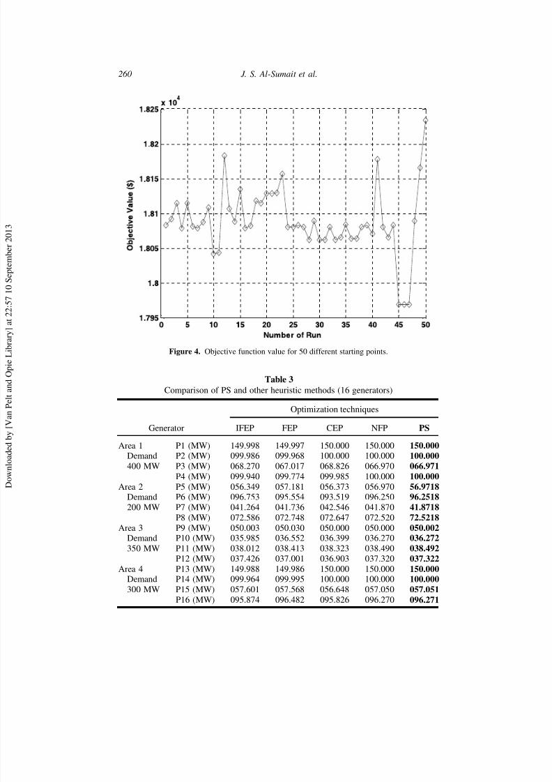
The PS has determined the optimal solution for 50 different initial points. The

solutions of each run are shown in Figure 4. The total execution time for the 50 runs

Figure 2. Convergence of PS for the 13 generating units.

7/29/2019 15325000701603892 powersys



Figure 3. Convergence of PS mesh size for the 13 generating units.

was 294.06 s. For this test case, looking at the maximum, mean, and minimum costs in

Table 2, it may be clearly seen that PS outperforms GA and evolutionary programming

(EP) by reaching a lower value of the maximum and mean costs for 50 different runs.

Case II: MAED

The MAED problem considered consists of four areas with tie lines connecting these

areas. Each area contains four generation units. Note that quadratic cost functions areused to model the cost of generation F .P gi /, but the tie line transmission costs, G.tjk/,

are assumed to be linear functions of the power transfer. The generators’ data and the tie

lines’ coefficients, along with their limits, are all given in [14].

Different heuristic methods, such as particle swarm optimization (PSO) and EP, have

been applied to the same problem, and the results are reported in [34, 35]. The resultsusing the PS and other methods are shown in Tables 3 and 4. The optimal solution

obtained by PS is obviously better than those obtained by various EP algorithms and issimilar to the result obtained by network flow programming (NFP) [14], which is not

heuristic in nature. In addition, the computation time of PS is less than the execution

times of the variants of EP.As illustrated in Figure 5, PS has located the optimal solution after only 200

iterations, but it continues computating and refining the result. Figure 6 shows the mesh

size expansion and contraction behavior during the PS search for the global minimum.

7/29/2019 15325000701603892 powersys



Figure 4. Objective function value for 50 different starting points.

Table 3

Comparison of PS and other heuristic methods (16 generators)

Optimization techniques

Generator IFEP FEP CEP NFP PS

Area 1 P1 (MW) 149.998 149.997 150.000 150.000 150.000Demand P2 (MW) 099.986 099.968 100.000 100.000 100.000

400 MW P3 (MW) 068.270 067.017 068.826 066.970 066.971

P4 (MW) 099.940 099.774 099.985 100.000 100.000


200 MW P7 (MW) 041.264 041.736 042.546 041.870 41.8718

P8 (MW) 072.586 072.748 072.647 072.520 72.5218


350 MW P11 (MW) 038.012 038.413 038.323 038.490 038.492P12 (MW) 037.426 037.001 036.903 037.320 037.322


300 MW P15 (MW) 057.601 057.568 056.648 057.050 057.051

P16 (MW) 095.874 096.482 095.826 096.270 096.271

7/29/2019 15325000701603892 powersys



Table 4

Comparison of PS and other heuristic methods (tie lines)

Area Tie lines values (MW)

From To IFEP FEP CEP NFP PS

1 2 00.094 00.062 00.000 00.000 00.000

1 3 18.649 18.241 19.587 18.180 18.181

1 4 00.000 00.000 00.000 00.000 00.000

2 1 00.018 00.000 00.018 00.000 00.000

2 3 69.997 69.790 68.861 69.730 69.730

2 4 00.000 00.000 00.000 00.000 00.000

3 1 00.000 00.000 00.000 00.000 00.000

3 2 00.000 00.000 00.000 00.000 00.000

3 4 00.000 00.000 00.000 00.000 00.000

4 1 00.549 01.548 00.758 01.210 01.2104 2 02.951 02.509 01.789 02.110 02.111

4 3 99.927 99.974 99.927 100.00 100.00

Total cost ($/h) 7337.51 7337.52 7337.75 7337.0 7336.98

Computation time (s) 23.97 7.47 7.82/11.49 — 5.77

Population size 100 100 100 — —

No. of iterations 585 645 758/920 — 1225

Figure 5. Convergence of PS for MAED.

7/29/2019 15325000701603892 powersys



Figure 6. Mesh size.

Case III: CEED

In this combined environmental ED case, a six-generator system is considered. Infor-

mation about the generators’ fuel cost, NOx emission functions, the B matrix, loss

coefficients, and the operating limits are detailed in [36]. The total load demand is set to

700 MW, and the weighting factor is 0.5.

The PS results of the line losses, emission, fuel cost, total cost, and computationtime are presented and compared with results of other heuristic methods (GA and EP

from [34, 35]) in Table 5. It can be seen that PS has reached the best total and fuel costs,

and also has produced the best time of computation compared with the other methods. In

addition, PS came third in line losses and emissions. The convergence of the PS needs

only 40 iterations and 2.05 s to reach the optimal solution, which are significantly lessfor EP and GA.

Case IV: QCFED

According to [17], it is an industry practice to adopt a cubic polynomial for modeling

fuel costs of generation units. This is particularly important in situations with generationunits having non-monotonically increasing incremental curves [19]. In this case, a three-

generator system is considered with third-order cost functions. Information about thegenerators’ fuel-cost coefficients, the B matrix, loss coefficients, and the operating limits

are detailed in [18].

The optimal solution of PS is given in Table 6, along with the results obtained byconventional DP from [18] for comparison purposes. Clearly, the PS has converged to a

better solution, while the execution time is less than 1 s. Also, the significant reduction

in line losses is obvious.

7/29/2019 15325000701603892 powersys



Table 5

Comparison of PS and other heuristic methods

Optimization techniques

Generator IFEP FEP CEP FCGA PS

P1 (MW) 077.142 077.358 077.274 080.16 77.4318

P2 (MW) 049.925 049.669 049.639 053.71 048.894

P3 (MW) 048.764 048.316 048.535 040.93 048.516

P4 (MW) 103.486 104.369 103.525 116.23 104.5679

P5 (MW) 259.805 260.663 260.695 251.20 260.8632

P6 (MW) 191.828 190.473 191.233 190.62 190.6723

Line losses (MW) 30.949 30.849 30.901 32.850 30.945

Emission (kg/h) 530.5164 532.5046 524.49 527.46 528.33

Fuel cost ($/h) 38,214.02 38,214.23 38,216.47 38,408.82 38,208.63

Total cost ($/h) 19,369.84 19,369.89 19,369.84 19,468.14 19,368.48

Computation time (s) 3.874 1.598 4.48 — 2.05

No. of iterations 57 65 77 — 40

FCGA: Fuzzy controlled genetic algorithm.

Table 6

Comparison of PS and DP with total demand

1400 MW

Optimization technique

Generator DP PS

P1 (MW) 360.2 372.29

P2 (MW) 406.4 356.0

P3 (MW) 676.8 712.0

Line losses (MW) 43.4 40.29

Fuel cost ($/h) 6642.26 6639.01

Computation time (s) — 0.619

No. of iterations 5 6

5. Conclusions

This paper introduces a new approach based on PS optimization to solve various prob-

lems of power system ELD. The proposed method has been applied to four types of

problems, including the EDVP effects, MAED, CEED, and QCFED. Through extensivecomparisons, it has been demonstrated that the PS approach outperforms other heuristic

methods in terms of reaching a better optimal solution; at the same time, the simplicity of the PS process makes the algorithm computationally more efficient. However, the PS is

more sensitive than the GA or EP to the initial guess (starting point) and appears to rely

more heavily on how close the given initial point is to the expected optimum. This, inturn, makes the PS method more susceptible to getting trapped in local minima. Overall,

the PS approach has been found to be a very efficient technique to study a wide range

of optimization problem in the area of power system.

7/29/2019 15325000701603892 powersys



Acknowledgment

This work has been supported by the government of The State of Kuwait, Public Authority

of Applied Science & Training, Kuwait (Project # TS-06-02).

References

1. Adler, R. B., and Fischl, R., “Security constrained economic dispatch with participation factors

based on worst case bus load variations,” IEEE Transactionson: Power Apparatus and Systems,

Vol. 96, pp. 347–356, 1977.

2. Bui, R. T., and Ghaderpanah, S., “Real power rescheduling and security assessment,” IEEE

Trans. Power Apparatus Syst., Vol. PAS-101, pp. 2906–2915, 1982.

3. Pancholi, R. K., and Swarup, K. S., “Particle swarm optimization for security constrained eco-

nomic dispatch,” International Conference on Intelligent Sensing and Information Processing,

Chennai, India, pp. 7–12, 2004.

4. El-Sharkawy, M., and Nieebur, D., “Artificial neural networks with application to power

systems,” IEEE Power Engineering Society, A Tutorial Course, 1996.

5. Yalcinoz, T., and Short, M. J., “Neural networks approach for solving economic dispatch

problem with transmission capacity constraints,” IEEE Trans. Power Syst., Vol. 13, pp. 307–

313, 1998.

6. Youssef, H. K., and El-Naggar, K. M., “Genetic based algorithm for security constrained power

system economic dispatch,” Elec. Power Syst. Res., Vol. 53, pp. 47–51, 2000.

7. Chen, C. L., and Chen, N., “Direct search method for solving economic dispatch problem

considering transmission capacity constraints,” IEEE Trans. Power Syst., Vol. 16, pp. 764–

769, 2001.

8. Hooke, R., and Jeeves, T. A., “Direct search solution of numerical and statistical problems,”

J. Assoc. Computing Mach., Vol. 8, pp. 212–229, 1961.

9. Lewis, R. M., Torczon, V., and Trosset, M. W., “Direct search methods: Then and now,” J.

Computat. Appl. Math., Vol. 124, pp. 191–207, 2000.

10. Deb, K., Optimization for Engineering Design: Algorithms and Examples, New Delhi: Prentice

Hall, 1995.

11. Walters, D. C., and Sheble, G. B., “Genetic algorithm solution of economic dispatch with

valve point loading,” IEEE Trans. Power Syst., Vol. 8, pp. 1325–1332, 1993.

12. Victoire, T. A. A., and Jeyakumar, A. E., “Hybrid PSO-SQP for economic dispatch with

valve-point effect,” Elec. Power Syst. Res., Vol. 71, pp. 51–59, 2004.

13. Victoire, T. A. A., and Jeyakumar, A. E., “A modified hybrid EP-SQP approach for dynamic

dispatch with valve-point effect,” Int. J. Elec. Power Energy Syst., Vol. 27, pp. 594–601, 2005.

14. Streiffert, D., “Multi-area economic dispatch with tie line constraints,” IEEE Trans. Power

Syst., Vol. 10, pp. 1946–1951, 1995.

15. Farag, A., Al-Baiyat, S., and Cheng, T. C., “Economic load dispatch multiobjective optimiza-

tion procedures using linear programming techniques,” IEEE Trans. Power Syst., Vol. 10,

pp. 731–738, 1995.

16. Song, Y. H., Wang, G. S., Wang, P. Y., and Johns, A. T., “Environmental/economic dispatch

using fuzzy logic controlled genetic algorithms,” IEE Proc. Generat. Transm. Distribut.,

Vol. 144, pp. 377–382, 1997.

17. Liang, Z. X., and Glover, J. D., “Improved cost functions for economic dispatch compensa-

tions,” IEEE Trans. Power Syst., Vol. 6, pp. 821–829, 1991.

18. Liang, Z. X., and Glover, J. D., “A zoom feature for a dynamic programming solution to

economic dispatch including transmission losses,” IEEE Trans. Power Syst., Vol. 7, pp. 544–

550, 1992.

19. Jiang, A., and Ertem, S., “Economic dispatch with non-monotonically increasing incremental

cost units and transmission system losses,” IEEE Trans. Power Syst., Vol. 10, pp. 891–897,

1995.

7/29/2019 15325000701603892 powersys



20. Saadat, H., Power System Analysis, Boston, MA/London: WCB/McGraw-Hill, 1999.

21. Grainger, J. J., and Stevenson, W. D., Power System Analysis, New York: McGraw-Hill, 1994.

22. Goldberg, D. E., Genetic Algorithms in Search, Optimization, and Machine Learning, Reading,

MA: Addison-Wesley, 1989.

23. Michalewicz, Z., Genetic Algorithms C Data Structures D Evolution Programs, 3rd rev. andextended ed., New York: Springer-Verlag, 1996.

24. Youssef, H. K., El-Shibini, M., and Hazaa, G. A., “Some new aspects in power system dynamic

security using pattern recognition,” Second Middle East Power Conference (MEPCON-92),

pp. 308–313, Egypt, January 1992.

25. Lewis, R. M., and Torczon, V., “A globally convergent augmented Lagrangian pattern search

algorithm for optimization with general constraints and simple bounds,” SIAM J. Optim.,

Vol. 12, pp. 1075–1089, 2001.

26. Conn, A. R., Gould, N. I. M., and Toint, P. L., “A globally convergent augmented Lagrangian

algorithm for optimization with general constraints and simple bounds,” SIAM J. Numer. Anal.,

Vol. 28, pp. 545–572, April 1991.

27. Conn, A. R., Gould, N. I. M., and Toint, P. L., “A globally convergent augmented Lagrangian

pattern search algorithm for optimization with general constraints and simple bounds,” Math.

Comput., Vol. 66, pp. 261–288, 1997.

28. Lewis, R. M., and Torczon, V., “Pattern search algorithms for linearly constrained minimiza-tion,” SIAM J. Optim., Vol. 10, pp. 917–941, 1999.

29. Lewis, R. M., and Torczon, V., “Pattern search algorithms for bound constrained minimization,”

SIAM J. Optim., Vol. 9, pp. 1082–1099, 1999.

30. Torczon, V., “On the convergence of pattern search algorithms,” SIAM J. Optim., Vol. 7,

pp. 1–25, 1997.

31. The Math Works Inc., Genetic Algorithm and Direct Search Toolbox for Use with Matlab

User’s Guide, 2nd ed.

32. Wong, K. P., and Wong, Y. W., “Thermal generator scheduling using hybrid genetic simulated-

annealing,” IEE Proc. Generat. Transm. Distrib., Vol. 142, pp. 372–380, July 1995.

33. Sinha, N., Chakrabarti, R., and Chattopadhyay, P. K., “Evolutionary programming techniques

for economic load dispatch,” IEEE Trans. Evolut. Comput., Vol. 7, pp. 83–94, 2003.

34. Jayabarathi, T., Jayaprakash, K., Jeyakumar, D. N., and Raghunathan, T., “Evolutionary pro-

gramming techniques for different kinds of economic dispatch problems,” Elec. Power Syst.

Res., Vol. 73, pp. 169–176, 2005.35. Jeyakumar, D. N., Jayabarathi, T., and Raghunathan, T., “Particle swarm optimization for

various types of economic dispatch problems,” Int. J. Elec. Power Energy Syst., Vol. 28,

pp. 36–42, 2006.

36. Dhillon, J. S., Parti, S. C., and Kothari, D. P., “Stochastic economic emission load dispatch,”

Elec. Power Syst. Res., Vol. 26, pp. 179–186, 1993.

15325000701603892 powersys

Documents