OUTLINE

1 Machine learning with neural networks . . . . . . . . . . . . . . . . . . . . . . . . . . . . . . . . . . . . . . . . . . . . . . . . . . . 3

2 Training neural networks . . . . . . . . . . . . . . . . . . . . . . . . . . . . . . . . . . . . . . . . . . . . . . . . . . . . . . . . . . . . . . . . 20

3 Popularity and applications . . . . . . . . . . . . . . . . . . . . . . . . . . . . . . . . . . . . . . . . . . . . . . . . . . . . . . . . . . . . . 37

2

OUTLINE

1 Machine learning with neural networks . . . . . . . . . . . . . . . . . . . . . . . . . . . . . . . . . . . . . . . . . . . . . . . . . . . 3

2 Training neural networks . . . . . . . . . . . . . . . . . . . . . . . . . . . . . . . . . . . . . . . . . . . . . . . . . . . . . . . . . . . . . . . . 20

3 Popularity and applications . . . . . . . . . . . . . . . . . . . . . . . . . . . . . . . . . . . . . . . . . . . . . . . . . . . . . . . . . . . . . 37

3

SUPERVISED MACHINE LEARNINGCLASSIFICATION SETUP

Input features x(i) ∈ Rn

Outputs y(i) ∈ Y (e.g. R, {−1,+1}, {1, . . . , p})

Model parameters θ ∈ Rk

Hypothesis function hθ : Rn → R

Loss function ` : R× Y→ R+

Machine learning optimization problem

minimizeθ

m∑i=1

`(hθ(x(i)), y(i))

4

LINEAR CLASSIFIERS

Linear hypothesis class:hθ(x

(i)) = θTφ(x(i))

where the input can be any set of non-linear features φ : Rn → Rk

The generic function φ represents some (possibly) selected way to generate non-linearfeatures out of the available ones, for instance:

x(i) = [temperature for day i]

φ(x(i)) =

1

x(i)

x(i)2

...

5

GENERAL REPRESENTATION OFLINEAR CLASSIFICATION

6

CHALLENGES WITH LINEAR MODELS

Linear models crucially depend on choosing “good” features

Some “standard” choices: polynomial features, radial basis functions, random features(surprisingly effective)

But, many specialized domains required highly engineered special features

E.g., computer vision tasks used Haar features, SIFT features, every 10 years or sosomeone would engineer a new set of features

Key question 1: Should we stick with linear hypothesis functions? What about usingnon-linear combinations of the inputs? → Feed-forward neural networks (Perceptrons)

Key question 2: can we come up with algorithms that will automatically learn thefeatures themselves? → Feed-forward neural networks with multiple (> 2!) hidden layers(Deep Networks)

7

FEATURE LEARNING:USE TWO CLASSIFIERS IN CASCADE

Instead of a simple linear classifier, let’s consider a two-stage hypothesis class where onelinear function creates the features, another models the classifier and takes as input thefeatures created by the first one:

hw(x) =W2φ(x) + b2 =W2(W1x+ b1) + b2

wherew = {W1 ∈ Rn×k, b1 ∈ Rk,W2 ∈ R1×k, b2 ∈ R}

Note that in this notation, we’re explicitly separating the parameters on the “constantfeature” into the b terms

8

FEATURE LEARNING:USE TWO CLASSIFIERS IN CASCADEGraphical depiction of the obtained function

x1

x2

xn

...

z1

z2

zk

...y

W1, b1

W2, b2

But there is a problem:

hw(x) =W2(W1x+ b1) + b2 = W̃x+ b̃ (1)

in other words, we are still just using a normal linear classifier: the apparent addedcomplexity by concatenating multiple is not giving us any additional representationalpower, we can only discriminate linearly separable classes

9

ARTIFICIAL NEURAL NETWORKS (ANN)

Neural networks provide a way to obtain complexity by:

1 Using non linear transformations of the inputs

2 Propagating the information among layers of processing units to realize multi-stagedcomputation

3 In deep networks, the number of stages is relatively large, allowing to automaticallylearn hierarchical representations of the data features

x1

x2

xn

...

z1

z2

zk

...y

W1, b1

W2, b2 z1 = x

......

W1, b1

z5... ...

z2 z3 z4

W3, b3

W4, b4

= hθ(x)

W2, b2

10

TYPICAL NON-LINEARACTIVATION FUNCTIONS

Using non-linear activation functions at each node, the two-layer network of the previousexample, become equivalent to have the following hypothesis function:

hθ(x) = f2(W2f1(W1x+ b1) + b2)

where f1, f2 : R→ R are some non-linear functions (applied elementwise to vectors)

Common choices for fi are hyperbolic tangent tanh(x) = (e2x − 1)/(e2x + 1),sigmoid/logistic σ(x) = 1/(1 + e−x), or rectified linear unit f(x) = max{0, x}

4 3 2 1 0 1 2 3 41.0

0.5

0.0

0.5

1.0tanh

4 3 2 1 0 1 2 3 40.0

0.2

0.4

0.6

0.8

1.0sigmoid

4 3 2 1 0 1 2 3 40.00.51.01.52.02.53.03.54.0

relu

11

HIDDEN LAYERSAND LEARNED FEATURES

We draw these the same as before (non-linear functions are virtually always implied in theneural network setting)

x1

x2

xn

...

z1

z2

zk

...y

W1, b1

W2, b2

Middle layer z is referred to as the hidden layer or activationsThese are the learned features, nothing in the data that prescribes what values theseshould take, left up to the algorithm to decideTo have a meaningful feature learning we need multiple hidden layers in cascadeNetworks

12

TYPES OF NETWORKS

13

PROPERTIES OF NEURAL NETWORKSIt turns out that a neural network with a single hidden layer (and a suitably large numberof hidden units) is a universal function approximator, can approximate any functionover the input arguments (but this is actually not very useful in practice, c.f. polynomialsfitting any sets of points for high enough degree)

The hypothesis class hθ is not a convex function of the parameters θ = {Wi, bi}

The number of parameters (weights and biases), layers (depth), topology (connectivity),activation functions, all affect the performance and capacity of the network

14

DEEP LEARNING

“Deep” neural networks refer to networks with multiple hidden layers

z1 = x

......

W1, b1

z5... ...

z2 z3 z4

W3, b3

W4, b4

= hθ(x)

W2, b2

Mathematically, a k-layer network has the hypothesis function

zi+1 = fi(Wizi + bi), i = 1, . . . , k − 1, z1 = x

hw(x) = zk

where zi terms now indicate vectors of output features

15

WHY USE DEEP NETWORKS?

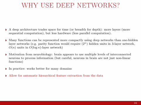
A deep architecture trades space for time (or breadth for depth): more layers (moresequential computation), but less hardware (less parallel computation).

Many functions can be represented more compactly using deep networks than one-hiddenlayer networks (e.g. parity function would require (2n) hidden units in 3-layer network,O(n) units in O(logn)-layer network)

Motivation from neurobiology: brain appears to use multiple levels of interconnectedneurons to process information (but careful, neurons in brain are not just non-linearfunctions)

In practice: works better for many domains

Allow for automatic hierarchical feature extraction from the data

16

HIERARCHICAL FEATUREREPRESENTATION

17

EXAMPLES OF HIERARCHICALFEATURE REPRESENTATION

18

EFFECT OF INCREASINGNUMBER OF HIDDEN LAYERS

Speech recognition task

19

OUTLINE

1 Machine learning with neural networks . . . . . . . . . . . . . . . . . . . . . . . . . . . . . . . . . . . . . . . . . . . . . . . . . . . 3

2 Training neural networks . . . . . . . . . . . . . . . . . . . . . . . . . . . . . . . . . . . . . . . . . . . . . . . . . . . . . . . . . . . . . . . . 20

3 Popularity and applications . . . . . . . . . . . . . . . . . . . . . . . . . . . . . . . . . . . . . . . . . . . . . . . . . . . . . . . . . . . . . 37

20

OPTIMIZING NEURAL NETWORKPARAMETERS

How do we optimize the parameters for the machine learning loss minimization problemwith a neural network

minimizeθ

m∑i=1

`(hθ(x(i)), y(i))

now that this problem is non-convex?

Just do exactly what we did before: initialize with random weights and run stochasticgradient descent

Now have the possibility of local optima, and function can be harder to optimize, but wewon’t worry about all that because the resulting models still often perform better thanlinear models

21

STOCHASTIC GRADIENT DESCENT FORNEURAL NETWORKS

Recall that stochastic gradient descent computes gradients with respect to loss on eachexample, updating parameters as it goes

function SGD({(x(i), y(i))}, hθ, `, α)Initialize: Wj , bj ← Random, j = 1, . . . , kRepeat until convergence:

For i = 1, . . . ,m:Compute ∇Wj ,bj `(hθ(x

(i)), y(i)), j = 1, . . . , k − 1

Take gradient steps in all directions:Wj ←Wj − α∇Wj

`(hθ(x(i)), y(i)), j = 1, . . . , k

bj ← bj − α∇bj `(hθ(x(i)), y(i)), j = 1, . . . , k

return {Wj , bj}

How do we compute the gradients ∇Wj ,bj `(hθ(x(i)), y(i))?

22

BACK-PROPAGATION

Back-propagation is a method for computing all the necessary gradients using oneforward pass (just computing all the activation values at layers), and one backwardpass (computing gradients backwards in the network)

The equations sometimes look complex, but it’s just an application of the chain rule ofcalculus and the use of Jacobians

23

JACOBIANS AND CHAIN RULEFor a multivariate, vector-valued function f : Rn → Rm, the Jacobian is a m× n matrix

(∂f(x)

∂x

)∈ Rm×n =

∂f1(x)∂x1

∂f1(x)∂x2

· · · ∂f1(x)∂xn

∂f2(x)∂x1

∂f2(x)∂x2

· · · ∂f2(x)∂xn

......

. . ....

∂fm(x)∂x1

∂fm(x)∂x2

· · · ∂fm(x)∂xn

For a scalar-valued function f : Rn → R, the Jacobian is the transpose of the gradient∂f(x)∂x

T= ∇xf(x)

For a vector-valued function, row i of the Jacobian corresponds to the gradient of thecomponent fi of the output vector, i = 1, . . . ,m. It tells how the variation of each inputvariable affects the variation of the output component

Column j of the Jacobian is the impact of the variation of the j-th input variable,j = 1, . . . , n, on each one of the m components of the output

Chain rule for the derivation of a composite function:

∂f(g(x))

∂x=∂f(g(x))

∂g(x)

∂g(x)

∂x

24

MULTI-LAYER / MULTI-MODULE FFMulti-layered feed-forward architecture(cascade): module/layer i gets as input thefeature vector xi−1 output from module i− 1,applies the transformation function Fi(xi−1,Wi),and produces the output xi

Each layer i contains (Nx)i parallel nodes(xi)j , j = 1, . . . , (Nx)i. Each node gets the inputfrom previous layer’s nodes through(Nx)i−1 ≡ (NW )i connections with weights(Wi)j , j = 1, . . . , (NW )i

Each layer learns its own weight vector Wi.

Fi is a vector function. At each node j of layer i,the transformation function is(Fi)j = f((Wi)

Tj · (xi−1)j) and f is the activation

function (e.g., a sigmoid), that can be safelyconsidered being the same for all nodes.

In the following the notation is made simpler bydropping the second indices and reasoning at theaggregate vector level of each layer.

25

FORWARD PROPAGATION

Forward Propagation:

Following the presentation of the traininginput x0, the output vectors xi resultingfrom the activation function Fi at all layersi = 1, . . . , n, are computed in sequence,starting from x1, and are stored

The output of the network, the loss ` (to beminimized), results from the forwardpropagation at output layer and computingthe deviation with respect to the target Y :

`(Y ,x,W ) = C(xn,Y )

26

COMPUTING GRADIENTS

At each iteration of SGD, the gradients withrespect to all the parameters of the system needto be computed (i.e., the weights Wi, that couldbe split in weights for input and weights for bias,but hereafter we just use the general form Wi)

After the Forward pass, let’s start setting up therelations for the Backward pass

Let’s consider the generic layer i: from theForward propagation, its output value is availableand is xi = Fi(xi−1,Wi)

In addition, let’s assume that we already know

∂`

∂xi,

that is, we know for each component of the vectorxi the variation of ` in relation to a variation ofxi. We can assume that we know ∂`

∂xisince we

will proceed backward

27

COMPUTING GRADIENTSSince we assume as known ∂`

∂xiand we have

computed xi = Fi(xi−1,Wi), we can use thechain rule to compute ∂`

∂Wi, which is the quantity

of interest, and which tells us the variation in ` asa response to a variation in the weights of Wi:

∂`

∂Wi=

∂`

∂xi

∂Fi(xi−1,Wi)

∂Wi

where xi is a substitute for Fi(xi−1,Wi)

Dimensionally, the previous equation is as follows:

[1×NW ] = [1×Nx] · [Nx ×NW ]

∂Fi(xi−1,Wi)

∂Wiis the Jacobian matrix of Fi with

respect to Wi

The element (k, l) of the Jacobian quantifies thevariation in the k-th output when a variation isexerted on the l-th weight[

∂Fi(xi−1,Wi)

∂Wi

]kl

=∂[Fi(xi−1,Wi)

]k

∂[Wi

]l

28

COMPUTING GRADIENTS

Let’s keep assuming that we known ∂`∂xi

and let’s use it

this time to compute ∂`∂xi−1

Applying the chain rule:

∂`

∂xi−1=

∂`

∂xi

∂Fi(xi−1,Wi)

∂xi−1

Dimensionally, the previous equation is as follows:

[1×Nx] = [1×Nx] · [Nx ×Nx]

∂Fi(xi−1,Wi)

∂xi−1is the Jacobian matrix of Fi with respect

to xi−1

The element (k, l) of the Jacobian quantifies thevariation in the k-th output when a variation is exertedon the l-th input

The equation above is a recurrence equation!

29

BACK-PROPAGATION (BP)To sequentially compute all the gradients needed bySGD, a backward sweep is applied, which is called theback-propagation algorithm, that precisely makesuse of the recurrence equation for ∂`

∂xi

1∂`

∂xn=∂C(xn,Y )

∂xn

2∂`

∂xn−1=

∂`

∂xn

∂Fn(xn−1,Wn)

∂xn−1

3∂`

∂Wn=

∂`

∂xn

∂Fn(xn−1,Wn)

∂Wn

4∂`

∂xn−2=

∂`

∂xn−1

∂Fn−1(xn−2,Wn−1)

∂xn−2

5∂`

∂Wn−1=

∂`

∂xn−1

∂Fn−1(xn−2,Wn−1)

∂Wn−1

6 . . . until we reach the first, input layer

7 → all the gradients∂`

∂Wi, ∀i = 1, . . . , n have been

computed!30

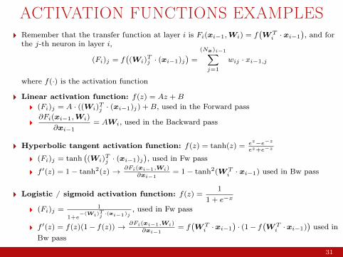
ACTIVATION FUNCTIONS EXAMPLESRemember that the transfer function at layer i is Fi(xi−1,Wi) = f

(W Ti · xi−1

), and for

the j-th neuron in layer i,

(Fi)j = f((Wi)

Tj · (xi−1)j

)=

(Nx)i−1∑j=1

wij · xi−1,j

where f(·) is the activation function

Linear activation function: f(z) = Az +B

(Fi)j = A · ((Wi)Tj · (xi−1)j) +B, used in the Forward pass

∂Fi(xi−1,Wi)

∂xi−1= AWi, used in the Backward pass

Hyperbolic tangent activation function: f(z) = tanh(z) = ez−e−z

ez+e−z

(Fi)j = tanh((Wi)

Tj · (xi−1)j

), used in Fw pass

f ′(z) = 1− tanh2(z) → ∂Fi(xi−1,Wi)

∂xi−1= 1− tanh2(W T

i · xi−1) used in Bw pass

Logistic / sigmoid activation function: f(z) =1

1 + e−x

(Fi)j = 1

1+e−(Wi)

Tj

·(xi−1)j, used in Fw pass

f ′(z) = f(z)(1− f(z)) → ∂Fi(xi−1,Wi)

∂xi−1= f

(W Ti ·xi−1

)· (1− f

(W Ti ·xi−1)

)used in

Bw pass

31

NO ARCHITECTURAL CONSTRAINTS

32

AVAILABLE TOOLS

Gradients can still get somewhat tedious to derive by hand, especially for the morecomplex models that follow

Fortunately, a lot of this work has already been done for you

Tools like Theano (http://deeplearning.net/software/theano/), Torch(http://torch.ch/), TensorFlow (http://www.tensorflow.org/) all let you specify thenetwork structure and then automatically compute all gradients (and use GPUs to do so)

Autograd package for Python (https://github.com/HIPS/autograd) lets you compute thederivative of (almost) any arbitrary function using numpy operations using automaticback-propagation

33

WHAT’S CHANGED SINCE THE 80S?

Most of these algorithms were developed in the 80s or 90s

So why are these just becoming more popular in the last few years?

More data

Faster computers (GPUs)

(Some) better optimization techniques

34

ISSUES

Vanishing gradients: as we add more and more hidden layers, back-propagationbecomes less and less useful in passing information to the lower layers. In effect, asinformation is passed back, the gradients begin to vanish and become small relative to theweights of the networks.

Each gradient assigns “credit” to each neuron i for the (mis)classification of the inputsample, however, credit depends (backward) on the average error associated to theneurons that take the output of i, such that going backward the credit has thetendency to vanish

If the activation function has a gradient “mostly” null, as in the case of sigmoids,then, again, gradient corrections become very small

Overfitting!

How many layers/nodes? (which is related to overfitting . . . )

Non-convexity (only local minimima can be reached), computation time, . . .

Time complexity of one BP iteration is O(|W |3), which is he input for one iteration ofSGD. No general guarantees on convergence time

35

IDEAS FOR OVERCOMING ISSUES

Hidden layers of autoencoders and RBMs act as effective feature detectors; thesestructures can be stacked to form deep networks. These networks can be trainedgreedily, one layer at a time, to help to overcome the vanishing gradient andoverfitting problems.

Unsupervised pre-training (Hinton et al., 2006): “Pre-train” the network have thehidden layers recreate their input, one layer at a time, in an unsupervised fashion

This paper was partly responsible for re-igniting the interest in deep neural networks,but the general feeling now is that it doesn’t help much

Dropout (Hinton et al., 2012): During training and computation of gradients,randomly set about half the hidden units to zero (a different randomly selected set foreach stochastic gradient step)

Acts like regularization, prevents the parameters for overfitting to particular examples

Different non-linear functions (Nair and Hinton, 2010): Use non-linearityf(x) = max{0, x} instead of f(x) = tanh(x)

36

OUTLINE

1 Machine learning with neural networks . . . . . . . . . . . . . . . . . . . . . . . . . . . . . . . . . . . . . . . . . . . . . . . . . . . 3

2 Training neural networks . . . . . . . . . . . . . . . . . . . . . . . . . . . . . . . . . . . . . . . . . . . . . . . . . . . . . . . . . . . . . . . . 20

3 Popularity and applications . . . . . . . . . . . . . . . . . . . . . . . . . . . . . . . . . . . . . . . . . . . . . . . . . . . . . . . . . . . . . 37

37

1980 1985 1990 1995 2000 2005 2010 20150.0

0.1

0.2

0.3

0.4

0.5

0.6#neural network / #machine learning

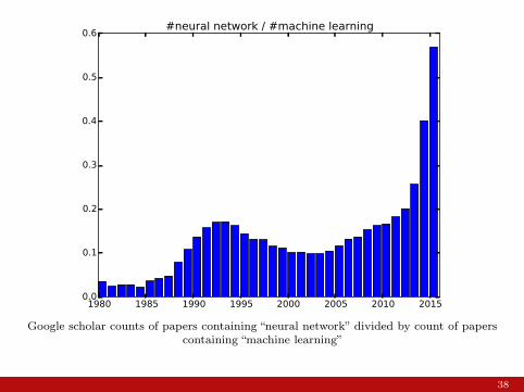
Google scholar counts of papers containing “neural network” divided by count of paperscontaining “machine learning”

38

Popularization of backpropfor training neural networks

Academic papers on unsupervisedpre-training for deep networks

“AlexNet” deep neural network wins ImageNet 2012 contest

Facebook launches AI researchcenter, Google buys DeepMind

A non-exhaustive list of some of the important events that impacted this trend

39

“AlexNet” (Krizhevsky et al., 2012), winning entry of ImageNet 2012 competition with aTop-5 error rate of 15.3% (next best system with highly engineered features based uponSIFT got 26.1% error)

Figure 2: An illustration of the architecture of our CNN, explicitly showing the delineation of responsibilitiesbetween the two GPUs. One GPU runs the layer-parts at the top of the figure while the other runs the layer-partsat the bottom. The GPUs communicate only at certain layers. The network’s input is 150,528-dimensional, andthe number of neurons in the network’s remaining layers is given by 253,440–186,624–64,896–64,896–43,264–4096–4096–1000.

neurons in a kernel map). The second convolutional layer takes as input the (response-normalizedand pooled) output of the first convolutional layer and filters it with 256 kernels of size 5 ⇥ 5 ⇥ 48.The third, fourth, and fifth convolutional layers are connected to one another without any interveningpooling or normalization layers. The third convolutional layer has 384 kernels of size 3 ⇥ 3 ⇥256 connected to the (normalized, pooled) outputs of the second convolutional layer. The fourthconvolutional layer has 384 kernels of size 3 ⇥ 3 ⇥ 192 , and the fifth convolutional layer has 256kernels of size 3 ⇥ 3 ⇥ 192. The fully-connected layers have 4096 neurons each.

4 Reducing Overfitting

Our neural network architecture has 60 million parameters. Although the 1000 classes of ILSVRCmake each training example impose 10 bits of constraint on the mapping from image to label, thisturns out to be insufficient to learn so many parameters without considerable overfitting. Below, wedescribe the two primary ways in which we combat overfitting.

4.1 Data Augmentation

The easiest and most common method to reduce overfitting on image data is to artificially enlargethe dataset using label-preserving transformations (e.g., [25, 4, 5]). We employ two distinct formsof data augmentation, both of which allow transformed images to be produced from the originalimages with very little computation, so the transformed images do not need to be stored on disk.In our implementation, the transformed images are generated in Python code on the CPU while theGPU is training on the previous batch of images. So these data augmentation schemes are, in effect,computationally free.

The first form of data augmentation consists of generating image translations and horizontal reflec-tions. We do this by extracting random 224⇥ 224 patches (and their horizontal reflections) from the256⇥256 images and training our network on these extracted patches4. This increases the size of ourtraining set by a factor of 2048, though the resulting training examples are, of course, highly inter-dependent. Without this scheme, our network suffers from substantial overfitting, which would haveforced us to use much smaller networks. At test time, the network makes a prediction by extractingfive 224 ⇥ 224 patches (the four corner patches and the center patch) as well as their horizontalreflections (hence ten patches in all), and averaging the predictions made by the network’s softmaxlayer on the ten patches.

The second form of data augmentation consists of altering the intensities of the RGB channels intraining images. Specifically, we perform PCA on the set of RGB pixel values throughout theImageNet training set. To each training image, we add multiples of the found principal components,

4This is the reason why the input images in Figure 2 are 224 ⇥ 224 ⇥ 3-dimensional.

5

40

Figure 4: (Left) Eight ILSVRC-2010 test images and the five labels considered most probable by our model.The correct label is written under each image, and the probability assigned to the correct label is also shownwith a red bar (if it happens to be in the top 5). (Right) Five ILSVRC-2010 test images in the first column. Theremaining columns show the six training images that produce feature vectors in the last hidden layer with thesmallest Euclidean distance from the feature vector for the test image.

In the left panel of Figure 4 we qualitatively assess what the network has learned by computing itstop-5 predictions on eight test images. Notice that even off-center objects, such as the mite in thetop-left, can be recognized by the net. Most of the top-5 labels appear reasonable. For example,only other types of cat are considered plausible labels for the leopard. In some cases (grille, cherry)there is genuine ambiguity about the intended focus of the photograph.

Another way to probe the network’s visual knowledge is to consider the feature activations inducedby an image at the last, 4096-dimensional hidden layer. If two images produce feature activationvectors with a small Euclidean separation, we can say that the higher levels of the neural networkconsider them to be similar. Figure 4 shows five images from the test set and the six images fromthe training set that are most similar to each of them according to this measure. Notice that at thepixel level, the retrieved training images are generally not close in L2 to the query images in the firstcolumn. For example, the retrieved dogs and elephants appear in a variety of poses. We present theresults for many more test images in the supplementary material.

Computing similarity by using Euclidean distance between two 4096-dimensional, real-valued vec-tors is inefficient, but it could be made efficient by training an auto-encoder to compress these vectorsto short binary codes. This should produce a much better image retrieval method than applying auto-encoders to the raw pixels [14], which does not make use of image labels and hence has a tendencyto retrieve images with similar patterns of edges, whether or not they are semantically similar.

7 Discussion

Our results show that a large, deep convolutional neural network is capable of achieving record-breaking results on a highly challenging dataset using purely supervised learning. It is notablethat our network’s performance degrades if a single convolutional layer is removed. For example,removing any of the middle layers results in a loss of about 2% for the top-1 performance of thenetwork. So the depth really is important for achieving our results.

To simplify our experiments, we did not use any unsupervised pre-training even though we expectthat it will help, especially if we obtain enough computational power to significantly increase thesize of the network without obtaining a corresponding increase in the amount of labeled data. Thusfar, our results have improved as we have made our network larger and trained it longer but we stillhave many orders of magnitude to go in order to match the infero-temporal pathway of the humanvisual system. Ultimately we would like to use very large and deep convolutional nets on videosequences where the temporal structure provides very helpful information that is missing or far lessobvious in static images.

8

Some classification results from AlexNet

41

Google Deep Dream software: adjust input images (by gradient descent) to strengthen theactivations that are present in an image

42

Question answering network (Vinyals and Le, 2015), using sequence to sequence learningmethod (Sutskever et al., 2014)A Neural Conversational Model

used for neural machine translation and achieves im-provements on the English-French and English-Germantranslation tasks from the WMT’14 dataset (Luong et al.,2014; Jean et al., 2014). It has also been used forother tasks such as parsing (Vinyals et al., 2014a) andimage captioning (Vinyals et al., 2014b). Since it iswell known that vanilla RNNs suffer from vanish-ing gradients, most researchers use variants of LongShort Term Memory (LSTM) recurrent neural net-works (Hochreiter & Schmidhuber, 1997).

Our work is also inspired by the recent success of neu-ral language modeling (Bengio et al., 2003; Mikolov et al.,2010; Mikolov, 2012), which shows that recurrent neuralnetworks are rather effective models for natural language.More recently, work by Sordoni et al. (Sordoni et al., 2015)and Shang et al. (Shang et al., 2015), used recurrent neuralnetworks to model dialogue in short conversations (trainedon Twitter-style chats).

Building bots and conversational agents has been pur-sued by many researchers over the last decades, and itis out of the scope of this paper to provide an exhaus-tive list of references. However, most of these systemsrequire a rather complicated processing pipeline of manystages (Lester et al., 2004; Will, 2007; Jurafsky & Martin,2009). Our work differs from conventional systems byproposing an end-to-end approach to the problem whichlacks domain knowledge. It could, in principle, be com-bined with other systems to re-score a short-list of can-didate responses, but our work is based on producing an-swers given by a probabilistic model trained to maximizethe probability of the answer given some context.

3. ModelOur approach makes use of the sequence-to-sequence(seq2seq) framework described in (Sutskever et al., 2014).The model is based on a recurrent neural network whichreads the input sequence one token at a time, and predictsthe output sequence, also one token at a time. During train-ing, the true output sequence is given to themodel, so learn-ing can be done by backpropagation. The model is trainedto maximize the cross entropy of the correct sequence givenits context. During inference, given that the true output se-quence is not observed, we simply feed the predicted outputtoken as input to predict the next output. This is a “greedy”inference approach. A less greedy approach would be touse beam search, and feed several candidates at the previ-ous step to the next step. The predicted sequence can beselected based on the probability of the sequence.

Concretely, suppose that we observe a conversation withtwo turns: the first person utters “ABC”, and second personreplies “WXYZ”. We can use a recurrent neural network,

Figure 1. Using the seq2seq framework for modeling conversa-tions.

and train to map “ABC” to “WXYZ” as shown in Figure 1above. The hidden state of the model when it receives theend of sequence symbol “<eos>” can be viewed as thethought vector because it stores the information of the sen-tence, or thought, “ABC”.

The strength of this model lies in its simplicity and gener-ality. We can use this model for machine translation, ques-tion/answering, and conversations without major changesin the architecture. Applying this technique to conversa-tion modeling is also straightforward: the input sequencecan be the concatenation of what has been conversed so far(the context), and the output sequence is the reply.

Unlike easier tasks like translation, however, a modellike sequence-to-sequence will not be able to successfully“solve” the problem of modeling dialogue due to sev-eral obvious simplifications: the objective function beingoptimized does not capture the actual objective achievedthrough human communication, which is typically longerterm and based on exchange of information rather than nextstep prediction. The lack of a model to ensure consistencyand general world knowledge is another obvious limitationof a purely unsupervised model.

4. DatasetsIn our experiments we used two datasets: a closed-domainIT helpdesk troubleshooting dataset and an open-domainmovie transcript dataset. The details of the two datasets areas follows.

4.1. IT Helpdesk Troubleshooting dataset

In our first set of experiments, we used a dataset which wasextracted from a IT helpdesk troubleshooting chat service.In this service, costumers face computer related issues, anda specialist help them by conversing and walking througha solution. Typical interactions (or threads) are 400 wordslong, and turn taking is clearly signaled. Our training setcontains 30M tokens, and 3M tokens were used as valida-tion. Some amount of clean up was performed, such asremoving common names, numbers, and full URLs.

A Neural Conversational Model

4.2. OpenSubtitles dataset

We also tested our model on the OpenSubtitlesdataset (Tiedemann, 2009). This dataset consists ofmovie conversations in XML format. It contains sen-tences uttered by characters in movies. We applied asimple processing step removing XML tags and obvi-ous non-conversational text (e.g., hyperlinks) from thedataset. As turn taking is not clearly indicated, we treatedconsecutive sentences assuming they were uttered bydifferent characters. We trained our model to predict thenext sentence given the previous one, and we did this forevery sentence (noting that this doubles our dataset size,as each sentence is used both for context and as target).Our training and validation split has 62M sentences (923Mtokens) as training examples, and the validation set has26M sentences (395M tokens). The split is done in such away that each sentence in a pair of sentences either appeartogether in the training set or test set but not both. Unlikethe previous dataset, the OpenSubtitles is quite large, andrather noisy because consecutive sentences may be utteredby the same character. Given the broad scope of movies,this is an open-domain conversation dataset, contrastingwith the technical troubleshooting dataset.

5. ExperimentsIn this section, we describe the experimental results withthe two datasets and show some samples of the interac-tions with the system that we trained. We also comparethe performance of our system against a popular rule-basedbot (CleverBot1) using human evaluations on a set of 200questions.

5.1. IT Helpdesk Troubleshooting experiments

In this experiment, we trained a single layer LSTM with1024 memory cells using stochastic gradient descent withgradient clipping. The vocabulary consists of the mostcommon 20K words, which includes special tokens indi-cating turn taking and actor.

At convergence, this model achieved a perplexity of 8,whereas an n-grammodel achieved 18. Below is a few sam-ples of simulated troubleshooting sessions for most threeof the most common IT problems (remote access, softwarecrashes, and password issues). In these conversations,Ma-chine is our Neural ConversationalModel, andHuman thehuman actor interacting with it.

Conversation 1: VPN issues.

Describe your problem: i am having issues ac-cessing vpn

1http://www.cleverbot.com/

Machine: hiHuman: helloMachine: could you please let me know what arethe operating systems you are using ?Human: i am using linuxMachine: ok it was in the ssl vpn on which youstated it was brokenMachine: please check if you are logged in tocorp networkMachine: what is the error that you are runningpleaseHuman: i am seeing an error related to vpnMachine: what is the error message that you aregetting when connecting to vpn using networkconnect ?Human: connection refused or something likethatMachine: may i know the version of networkconnect you connect ?Human: i am not sure i know thatMachine: is the network connect prompting forany user certificateMachine: ?Human: yesMachine: are you at home or at work at the mo-ment ?Machine: office ?Human: i am at homeMachine: try thisMachine: goto <URL> page and enter yourname and passwordHuman: doneMachine: try logging in with <NAME> andcheck if its working fine nowHuman: yes , now it works !Machine: greatMachine: anything else that i can helpHuman: no , that was very usefulMachine: you are other than <NAME> : )Machine: have a nice night

(The <URL> indeed contains information about vpn ac-cess.)

Conversation 2: Browser issues.

Describe your problem: browser keeps crashingMachine: hiHuman: hiMachine: could you please let me know what isthe operating system you are using ?Human: linuxMachine: ok this is the issue with the system per-formance , nasser , tools .Human: what is that ?

A Neural Conversational Model

4.2. OpenSubtitles dataset

We also tested our model on the OpenSubtitlesdataset (Tiedemann, 2009). This dataset consists ofmovie conversations in XML format. It contains sen-tences uttered by characters in movies. We applied asimple processing step removing XML tags and obvi-ous non-conversational text (e.g., hyperlinks) from thedataset. As turn taking is not clearly indicated, we treatedconsecutive sentences assuming they were uttered bydifferent characters. We trained our model to predict thenext sentence given the previous one, and we did this forevery sentence (noting that this doubles our dataset size,as each sentence is used both for context and as target).Our training and validation split has 62M sentences (923Mtokens) as training examples, and the validation set has26M sentences (395M tokens). The split is done in such away that each sentence in a pair of sentences either appeartogether in the training set or test set but not both. Unlikethe previous dataset, the OpenSubtitles is quite large, andrather noisy because consecutive sentences may be utteredby the same character. Given the broad scope of movies,this is an open-domain conversation dataset, contrastingwith the technical troubleshooting dataset.

5. ExperimentsIn this section, we describe the experimental results withthe two datasets and show some samples of the interac-tions with the system that we trained. We also comparethe performance of our system against a popular rule-basedbot (CleverBot1) using human evaluations on a set of 200questions.

5.1. IT Helpdesk Troubleshooting experiments

In this experiment, we trained a single layer LSTM with1024 memory cells using stochastic gradient descent withgradient clipping. The vocabulary consists of the mostcommon 20K words, which includes special tokens indi-cating turn taking and actor.

At convergence, this model achieved a perplexity of 8,whereas an n-grammodel achieved 18. Below is a few sam-ples of simulated troubleshooting sessions for most threeof the most common IT problems (remote access, softwarecrashes, and password issues). In these conversations,Ma-chine is our Neural ConversationalModel, andHuman thehuman actor interacting with it.

Conversation 1: VPN issues.

Describe your problem: i am having issues ac-cessing vpn

1http://www.cleverbot.com/

Machine: hiHuman: helloMachine: could you please let me know what arethe operating systems you are using ?Human: i am using linuxMachine: ok it was in the ssl vpn on which youstated it was brokenMachine: please check if you are logged in tocorp networkMachine: what is the error that you are runningpleaseHuman: i am seeing an error related to vpnMachine: what is the error message that you aregetting when connecting to vpn using networkconnect ?Human: connection refused or something likethatMachine: may i know the version of networkconnect you connect ?Human: i am not sure i know thatMachine: is the network connect prompting forany user certificateMachine: ?Human: yesMachine: are you at home or at work at the mo-ment ?Machine: office ?Human: i am at homeMachine: try thisMachine: goto <URL> page and enter yourname and passwordHuman: doneMachine: try logging in with <NAME> andcheck if its working fine nowHuman: yes , now it works !Machine: greatMachine: anything else that i can helpHuman: no , that was very usefulMachine: you are other than <NAME> : )Machine: have a nice night

(The <URL> indeed contains information about vpn ac-cess.)

Conversation 2: Browser issues.

Describe your problem: browser keeps crashingMachine: hiHuman: hiMachine: could you please let me know what isthe operating system you are using ?Human: linuxMachine: ok this is the issue with the system per-formance , nasser , tools .Human: what is that ?

43

AlphaGo (Silver et al., 2016) beats Lee Sedol in 5 game competition

44