15-744: computer networking l-13 sensor networks
TRANSCRIPT

15-744: Computer Networking
L-13 Sensor Networks

Sensor Networks
• Directed Diffusion
• Aggregation
• Assigned reading• TAG: a Tiny AGgregation Service for Ad-Hoc
Sensor Networks• Directed Diffusion: A Scalable and Robust
Communication Paradigm for Sensor Networks
2

Outline
• Sensor Networks
• Directed Diffusion
• TAG
• Synopsis Diffusion
3

4
Smart-Dust/Motes
• First introduced in late 90’s by groups at UCB/UCLA/USC• Published at Mobicom/SOSP conferences
• Small, resource limited devices• CPU, disk, power, bandwidth, etc.
• Simple scalar sensors – temperature, motion
• Single domain of deployment (e.g. farm, battlefield, etc.) for a targeted task (find the tanks)
• Ad-hoc wireless network

5
Smart-Dust/Motes
• Hardware• UCB motes
• Programming• TinyOS
• Query processing• TinyDB• Directed diffusion• Geographic hash tables
• Power management• MAC protocols• Adaptive topologies

• Devices that incorporate communications, processing, sensors, and batteries into a small package
• Atmel microcontroller with sensors and a communication unit • RF transceiver, laser
module, or a corner cube reflector
• Temperature, light, humidity, pressure, 3 axis magnetometers, 3 axis accelerometers
Berkeley Motes
6

7
Berkeley Motes (Levis & Culler, ASPLOS 02)

Sensor Net Sample Apps
8
Traditional monitoring apparatus.
Earthquake monitoring in shake-test sites.
Vehicle detection: sensors along a road, collect data about passing vehicles.
Habitat Monitoring: Storm petrels on great duck island, microclimates on James Reserve.

9
Metric: Communication
• Lifetime from one pair of AA batteries • 2-3 days at full power• 6 months at 2% duty
cycle
• Communication dominates cost• < few mS to compute• 30mS to send
message
Time v. Current Draw During Query Processing
0
5
10
15
20
0 0.5 1 1.5 2 2.5 3Time (s)
Cu
rre
nt
(mA
) Snoozing
Processing
Processingand Listening
Transmitting

10
Communication In Sensor Nets
• Radio communication has high link-level losses• typically about 20% @
5m
• Ad-hoc neighbor discovery
• Tree-based routing
A
B C
D
FE

Outline
• Sensor Networks
• Directed Diffusion
• TAG
• Synopsis Diffusion
11

The long term goal
12
Disaster ResponseCirculatory Net
EmbedEmbed numerous distributed devices to monitor and interact with physical world: in work-spaces, hospitals, homes, vehicles, and “the environment” (water, soil, air…)
Network these devices so that they can coordinate to perform higher-level tasks.
Requires robust distributed systems of tens of thousands of devices.

Motivation
• Properties of Sensor Networks• Data centric, but not node centric• Have no notion of central authority• Are often resource constrained
• Nodes are tied to physical locations, but:• They may not know the topology• They may fail or move arbitrarily
• Problem: How can we get data from the sensors?
13

Directed Diffusion
• Data centric – nodes are unimportant• Request driven:
• Sinks place requests as interests• Sources are eventually found and satisfy interests• Intermediate nodes route data toward sinks
• Localized repair and reinforcement• Multi-path delivery for multiple sources, sinks, and
queries
14

Motivating Example
• Sensor nodes are monitoring a flat space for animals
• We are interested in receiving data for all 4-legged creatures seen in a rectangle
• We want to specify the data rate
15

Interest and Event Naming• Query/interest:
1. Type=four-legged animal2. Interval=20ms (event data rate)3. Duration=10 seconds (time to cache)4. Rect=[-100, 100, 200, 400]
• Reply:1. Type=four-legged animal2. Instance = elephant3. Location = [125, 220]4. Intensity = 0.65. Confidence = 0.856. Timestamp = 01:20:40
• Attribute-Value pairs, no advanced naming scheme
16

Diffusion (High Level)
• Sinks broadcast interest to neighbors
• Interests are cached by neighbors
• Gradients are set up pointing back to where interests came from at low data rate
• Once a sensor receives an interest, it routes measurements along gradients
17

18
Illustrating Directed Diffusion
Sink
Source
Setting up gradients
Sink
Source
Sending data
Sink
Source
Recoveringfrom node failure
Sink
Source
Reinforcingstable path

Summary• Data Centric
• Sensors net is queried for specific data• Source of data is irrelevant• No sensor-specific query
• Application Specific• In-sensor processing to reduce data transmitted• In-sensor caching
• Localized Algorithms• Maintain minimum local connectivity – save energy• Achieve global objective through local coordination
• Its gains due to aggregation and duplicate suppression may make it more viable than ad-hoc routing in sensor networks
19

Outline
• Sensor Networks
• Directed Diffusion
• TAG
• Synopsis Diffusion
20

TAG Introduction• Programming sensor nets is hard!• Declarative queries are easy
• Tiny Aggregation (TAG): In-network processing via declarative queries
• In-network processing of aggregates• Common data analysis operation• Communication reducing
• Operator dependent benefit• Across nodes during same epoch
• Exploit semantics improve efficiency!
• Example: • Vehicle tracking application: 2 weeks for 2
students• Vehicle tracking query: took 2 minutes to
write, worked just as well!
21
SELECT MAX(mag) FROM sensors WHERE mag > threshEPOCH DURATION 64ms

Basic Aggregation
• In each epoch:• Each node samples local sensors once• Generates partial state record (PSR)
• local readings • readings from children
• Outputs PSR during its comm. slot.
• At end of epoch, PSR for whole network output at root
• (In paper: pipelining, grouping)
22
1
2 3
4
5

23
Illustration: Aggregation
1 2 3 4 5
1 1
2
3
4
1
1
2 3
4
5
1
Sensor #
Slo
t #
Slot 1SELECT COUNT(*) FROM sensors

24
Illustration: Aggregation
1 2 3 4 5
1 1
2 2
3
4
1
1
2 3
4
5
2
Sensor #
Slo
t #
Slot 2SELECT COUNT(*) FROM sensors

25
Illustration: Aggregation
1 2 3 4 5
1 1
2 2
3 1 3
4
1
1
2 3
4
5
31
Sensor #
Slo
t #
Slot 3SELECT COUNT(*) FROM sensors

26
Illustration: Aggregation
1 2 3 4 5
1 1
2 2
3 1 3
4 5
1
1
2 3
4
5
5
Sensor #
Slo
t #
Slot 4SELECT COUNT(*) FROM sensors

27
Illustration: Aggregation
1 2 3 4 5
1 1
2 2
3 1 3
4 5
1 1
1
2 3
4
5
1
Sensor #
Slo
t #
Slot 1SELECT COUNT(*) FROM sensors

28
Types of Aggregates
• SQL supports MIN, MAX, SUM, COUNT, AVERAGE
• Any function can be computed via TAG
• In network benefit for many operations• E.g. Standard deviation, top/bottom N, spatial
union/intersection, histograms, etc. • Compactness of PSR

Taxonomy of Aggregates
• TAG insight: classify aggregates according to various functional properties• Yields a general set of optimizations that can
automatically be applied
29
Property Examples AffectsPartial State MEDIAN : unbounded,
MAX : 1 recordEffectiveness of TAG
Duplicate Sensitivity
MIN : dup. insensitive,AVG : dup. sensitive
Routing Redundancy
Exemplary vs. Summary
MAX : exemplaryCOUNT: summary
Applicability of Sampling, Effect of Loss
Monotonic COUNT : monotonicAVG : non-monotonic
Hypothesis Testing, Snooping
30
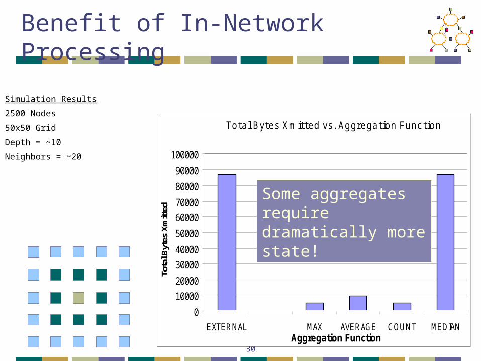
Benefit of In-Network Processing
Total Bytes Xmitted vs. Aggregation Function
0
10000
20000
30000
40000
50000
60000
70000
80000
90000
100000
EXTERNAL MAX AVERAGE COUNT MEDIANAggregation Function
Tota
l Byt
es X
mitt
ed
Simulation Results
2500 Nodes
50x50 Grid
Depth = ~10
Neighbors = ~20
Some aggregates require dramatically more state!

31
Optimization: Channel Sharing (“Snooping”)
• Insight: Shared channel enables optimizations
• Suppress messages that won’t affect aggregate• E.g., MAX• Applies to all exemplary, monotonic aggregates

Optimization: Hypothesis Testing
• Insight: Guess from root can be used for suppression• E.g. ‘MIN < 50’• Works for monotonic & exemplary aggregates
• Also summary, if imprecision allowed
• How is hypothesis computed?• Blind or statistically informed guess• Observation over network subset
32

Optimization: Use Multiple Parents
• For duplicate insensitive aggregates
• Or aggregates that can be expressed as a linear combination of parts• Send (part of) aggregate to all parents
• In just one message, via broadcast
• Decreases variance
33A
B C
A
B C
A
B C
1
A
B C
A
B C
1/2 1/2

34
Multiple Parents Results
• Better than previous analysis expected!
• Losses aren’t independent!
• Insight: spreads data over many links
Benefit of Result Splitting (COUNT query)
0
200
400
600
800
1000
1200
1400
(2500 nodes, lossy radio model, 6 parents per node)
Avg
. C
OU
NT Splitting
No Splitting
Critical Link!
No Splitting With Splitting

Outline
• Sensor Networks
• Directed Diffusion
• TAG
• Synopsis Diffusion
35

36
Aggregation in Wireless Sensors
Aggregate data is often more important
1 1
31
1
371
2 1
103Count =
In-network aggregation over tree with unreliable communication
Not robust against node- or link-failures
Used by current systems, TinyDB [Madden et al. OSDI’02] Cougar [Bonnet et al. MDM’01]
10

37
Traditional Approach
• Reliable communication• E.g., RMST over Directed Diffusion [Stann’03]
• High resource overhead• 3x more energy consumption
• 3x more latency
• 25% less channel capacity
• Not suitable for resource constrained sensors

38
Exploiting Broadcast Medium
Robust multi-path Energy-efficient
14
715
2
20 23Count =
1
3
2
58
Double-countingDifferent ordering
Challenge: order and duplicate insensitivity(ODI)
10
Challenge

39
A Naïve ODI Algorithm
• Goal: count the live sensors in the network
0 1 0 0 0 0 0 0 0 0 1 0
0 0 1 0 0 0 0 0 0 0 0 1
idBit vector

40
Synopsis Diffusion (SenSys’04)
• Goal: count the live sensors in the network
0 1 0 0 0 0 0 0 0 0 1 0
0 0 1 0 0 0 0 0 0 0 0 1
idBit vector0 1 0 0 0 0 Boolean
OR0 1 0 0 1 0
0 1 1 0 0 0
0 1 0 0 0 0 0 1 0 0 1 0
0 1 1 0 1 0
0 1 0 0 1 0
0 1 0 0 1 1
0 1 1 0 1 1Count 1 bits4
Synopsis should be small
Approximate COUNT algorithm: logarithmic size bit vector
Challenge

41
Synopsis Diffusion over Rings
• Each node transmits once = optimal energy cost (same as Tree)
Ring 2
• A node is in ring i if it is i hops away from the base-station
• Broadcasts by nodes in ring i are received by neighbors in ring i-1

42
Evaluation
Approximate COUNT with Synopsis Diffusion
Scheme Energy
Tree 41.8 mJ
Syn. Diff. 42.1 mJ
0
0.25
0.5
0.75
1
0 0.25 0.5 0.75 1
Loss Rate
RM
S E
rro
r
Tree Syn. Diff.
More robust than TreeAlmost as energy efficient as Tree
Per node energy
Typicalloss rates