| T H E A U S T R A L I A N N A T I O N A L U N I V E R S I T Y

1

Crawford School of Public Policy

2

Centre for Climate Economic & Policy

Towards a more inclusive and precautionary indicator of global sustainability

CCEP Working Paper 1410 July 2014 John C. V. Pezzey Fenner School of Environment and Society, The Australian National University Paul J. Burke Crawford School of Public Policy, The Australian National University Abstract We construct a hybrid, economic indicator of the sustainability of global well-being, which is more inclusive than existing indicators and incorporates an environmentally pessimistic, physical constraint on global warming. Our methodology extends the World Bank’s Adjusted Net Saving (ANS) indicator to include the cost of population growth, the benefit of technical progress, and a much higher, precautionary cost of current CO2 emissions. Future warming damage is so highly unknowable that valuing emissions directly is rather arbitrary, so we use a novel, inductive approach: we modify damage and climate parameters in the deterministic DICE climate-economy model so it becomes economically optimal to control emissions in a way likely to limit warming to an agreed target, here 2°C. If future emissions are optimally controlled, our ANS then suggests that current global well-being is sustainable. But if emissions remain uncontrolled, our base-case ANS is negative now and our corresponding, modified DICE model has an unsustained development path, with well-being peaking in 2065. Current ANS on an uncontrolled path may thus be a useful heuristic indicator of future unsustainability. Our inductive method might allow ANS to include other very hard-to-value, environmental threats to global sustainability, like biodiversity loss and nitrogen pollution.

| T H E A U S T R A L I A N N A T I O N A L U N I V E R S I T Y

Keywords global sustainability; optimism and pessimism; precautionary valuation of CO2 emissions; unknowability and induction; population growth; technical progress JEL Classification Q56, Q01, Q57, Q51, Q54, Q55 Suggested Citation: Pezzey, J. and Burke, P. (2014), Towards a more inclusive and precautionary indicator of global sustainability, CCEP Working Paper 1410, July 2014. Crawford School of Public Policy, The Australian National University. Address for correspondences: John C. V. Pezzey Senior Fellow Fenner School of Environment and Society The Australian National University Canberra ACT 0200 Tel: +61 2 6125 4143 Email: jack.pezzey@anu.edu.au

The Crawford School of Public Policy is the Australian National University’s public policy school, serving and influencing Australia, Asia and the Pacific through advanced policy research, graduate and executive education, and policy impact. The Centre for Climate Economics & Policy is an organized research unit at the Crawford School of Public Policy, The Australian National University. The working paper series is intended to facilitate academic and policy discussion, and the views expressed in working papers are those of the authors. Contact for the Centre: Dr Frank Jotzo, frank.jotzo@anu.edu.au

1

Towards a more inclusive and precautionary indicator of global sustainability

John C. V. Pezzeya,*, Paul J. Burkeb

a Fenner School of Environment and Society, Australian National University, Canberra, ACT

0200, Australia b Crawford School of Public Policy, Australian National University, Canberra, ACT 0200,

Australia

*Corresponding author at: Fenner School of Environment and Society, Australian National University, Canberra, ACT

0200, Australia. Tel.: + 61 2 6125 4143. E-mail: jack.pezzey@anu.edu.au

July 2014

ABSTRACT

We construct a hybrid, economic indicator of the sustainability of global well-being, which is more

inclusive than existing indicators and incorporates an environmentally pessimistic, physical

constraint on global warming. Our methodology extends the World Bank’s Adjusted Net Saving

(ANS) indicator to include the cost of population growth, the benefit of technical progress, and a

much higher, precautionary cost of current CO2 emissions. Future warming damage is so highly

unknowable that valuing emissions directly is rather arbitrary, so we use a novel, inductive

approach: we modify damage and climate parameters in the deterministic DICE climate-economy

model so it becomes economically optimal to control emissions in a way likely to limit warming to

an agreed target, here 2 oC. If future emissions are optimally controlled, our ANS then suggests

that current global well-being is sustainable. But if emissions remain uncontrolled, our base-case

ANS is negative now and our corresponding, modified DICE model has an unsustained

development path, with well-being peaking in 2065. Current ANS on an uncontrolled path may

thus be a useful heuristic indicator of future unsustainability. Our inductive method might allow

ANS to include other very hard-to-value, environmental threats to global sustainability, like

biodiversity loss and nitrogen pollution.  

Keywords:  global   sustainability;  optimism  and  pessimism;  precautionary  valuation  of  CO2  emissions;  unknowability  and  induction;  population  growth;  technical  progress  

2

1. Introduction

Are current levels of global human well-being sustainable for at least a century, if

depletion of the planet’s environmental resources is optimally controlled in future? Is

rising global well-being unsustainable for another century or so, if business-as-usual

trends in largely uncontrolled depletion of environmental resources continue? Asking

these two questions about global sustainability tackles one of humanity’s most

complex and persistent debates, where most contributions (e.g., Meadows et al., 1972;

Nordhaus, 1973) belong to one of two opposing paradigms (Neumayer, 2013). The

first paradigm can be broadly labelled “substitutability” (of human-made inputs for

environmental resource inputs in producing output and well-being), “weak

sustainability”,1 or “environmental optimism”, though these labels do not have

identical meanings. The second can be broadly labelled “non-substitutability”,

“strong sustainability”, or “environmental pessimism”. A key reason why they

persistently disagree is that “support for one paradigm or the other depends much on

basic beliefs ... that are non-falsifiable and cannot therefore be conclusively decided”

(Neumayer, 2013: 3). We therefore use “optimism” and “pessimism” here purely

non-judgmentally, just to describe the paradigms.

Because of these non-falsifiable disagreements, some authorities recommend

informing policy debates by presenting multiple sustainability indicators from

different paradigms (e.g., Stiglitz et al., 2009). As an alternative, we make a first

attempt at developing here a single, policy-relevant, empirical indicator of global

sustainability, that is more inclusive than existing indicators in three ways. First, it

includes more determinants of global sustainability than have yet been combined in

any single indicator. Second, it includes elements of both optimistic and pessimistic

paradigms, and so in some sense attempts to bridge the gulf between them in order to

better inform policy-makers, who cannot subscribe to different planets like academics

subscribe to different paradigms. Third, our indicator can be applied to both our

1 An even “weaker” paradigm is mainstream growth economics, which almost completely ignores

environmental resources. For instance, only one paper (Brock and Taylor, 2010) out of 121 during

2004-13 in the prestigious Journal of Economic Growth considered global warming or energy inputs.

3

opening questions, about global sustainability under optimal control, or under

negligible future control, of the environment.

Our focus on building a single, inclusive, and policy-relevant indicator leads us to

use a novel, experimental methodology, which is perhaps more the contribution of

this paper than the particular numerical results shown here. We change and extend

the empirical indicator of global sustainability that is already most inclusive and

policy-relevant. This is the global result for the World Bank’s Adjusted Net Savings

(ANS, also known as Genuine Saving) indicator, which the Bank estimates for over

120 countries (World Bank, 2006, 2011). Derived from conventional, “weak”

economic theory, ANS estimates how well any society is currently maintaining all its

human-made and natural assets. ANS assumes smooth substitutability among and

optimal control of all inputs, which allows it to serve as a sustainability indicator,

albeit an inexact one (Hamilton, 1994; Hamilton and Clemens, 1999; Pezzey, 2004),

where sustainability is defined as society being able to sustain current, average well-

being indefinitely (Pezzey, 1997). Our global application of this definition ignores

the requirement for more equity within and between nations that many authors

consider a vital part of sustainable development, and avoids the need to consider

international trade. We also ignore possible non-environmental impacts on long-run

global well-being, such as from nuclear war, disease, or asteroids.

Data and computational limits mean that the World Bank does not estimate ANS

from a separate, complete empirical model for each country. Instead, each estimate is

a hybrid: it adds together direct valuations from different sources, using market-based

prices (including discount rates) if available, and modelling results if not, a process

which inevitably entails broad approximations and many omissions. Our indicator

hybridizes World Bank ANS further, by replacing its (weak, optimistic) valuation of

the current CO2 emissions causing future global warming with much higher,

precautionary valuations. We calculate these valuations by backwards induction from

a physical (strong, pessimistic) target of limiting warming to the globally agreed

Copenhagen 2 oC limit (UN, 2009). However, discount rates in our inductive method

are still market-based and very similar to the World Bank’s. In that sense we are

4

interpreting the 2 oC limit as meaning the aim of climate policy is to protect future

generations from global warming damage, rather than to increase general

intergenerational concern. The second interpretation merits further research but is

beyond our scope here.

In addition to changing the World Bank’s CO2 valuation for ANS, we also extend

their ANS by including fairly conventional estimates of the cost of exogenous

population growth, currently not reported globally, and the benefit of exogenous

technical progress, currently omitted. According to these estimates, the sustainability

cost of population growth, assumed to be at a constant rate, is generally outweighed

by the sustainability benefit of technical progress. Our modifications to ANS are thus

not a uniform shift towards environmental pessimism. And our two extensions would

be impossible to make with pessimistic, biophysical, “strong” indicators of global

environmental impacts, such as the Ecological Footprint or Living Planet Index (e.g.,

WWF, 2012), Human Appropriation of Net Primary Production (e.g., Krausmann et

al., 2013), or Energy Return On Investment (e.g., Gagnon et al., 2009). These were

never designed to include all determinants of well-being, and cannot be extended to

do so.

As detailed later, our precautionary, inductive method for revaluing CO2

emissions entails finding parameters for climate damage, climate sensitivity, and non-

CO2 radiative forcing that will, in a deterministic, integrated assessment (global

climate-economy) model (IAM), make it economically optimal to control emissions

enough to be likely (give about a two-thirds chance, reflecting moderate risk aversion)

to limit peak global warming to 2 oC.2 The IAM we use is a modified version of

DICE-2007, Nordhaus’s (2008) version of his Dynamic Integrated model of Climate

and the Economy, hereafter DICE or standard DICE unless ambiguity arises.

Inductive approaches have been used before in climate economics to induce model

parameters from policy goals, for example by Gjerde et al. (1999), though they

included the well-being (pure time) discount rate as one of the parameters modified. 2 Other warming limits could readily be used with our approach, and may need to be, given the ever-

increasing difficulty of staying within 2 oC (e.g., Guivarch and Hallegatte, 2013).

5

Running the base case of our inductively modified DICE model with either optimal

control or no control of CO2 emissions then yields two very different social costs of

current CO2 emissions (SCCs): $131 per ton of carbon (/tC) under optimal control,

and $1,455/tC under no control, where “$” always means US2005$. These are much

higher than DICE or World Bank SCCs; but our no-control SCC is exceeded by some

in the economics literature (e.g., ~$94,000/tC in Howarth et al., 2014), and by the

infinite SCC implied by the absolute “non-substitutability” language used in most

“strong sustainability” literature. Our modified DICE also yields two valuations of

technical progress, and inserting these and the CO2 valuations into an extended World

Bank ANS addresses, though unsurprisingly does not answer conclusively, our two

opening questions about global sustainability.

Throughout the paper we discuss the validity of different parts of our

methodology. In particular, our use of induction in a deterministic IAM to revalue

CO2 emissions is contentious enough to warrant extensive discussion below, with a

summary here. We judge that the World Bank’s SCC of $24.5/tC is inconsistent with

recent warnings from climate scientists about dangerous global warming, and so

should be replaced with a more precautionary value. But we depart from the

conventional view that economic modelling should be used to estimate directly how

much warming should be permitted, because of a second judgment, that climate

damage is highly, but not absolutely, unknowable, especially at high warming levels.

All climate damage functions in existing IAMs therefore use essentially arbitrary

guesswork at high warming levels. So inducing an SCC from the knowledge inherent

in the consensus 2 oC target is not necessarily any less coherent, and is worth trying as

an alternative. And our somewhat paradoxical use of a deterministic IAM, despite

high unknowability, makes our key assumptions easier to find and contend than if we

used a more complex, probabilistic IAM.

Inductive valuation also opens the important possibility of including in ANS other

“strong”, physical limits to global sustainability, such as the “planetary boundaries”

for biodiversity loss or for human conversion of atmospheric nitrogen to reactive

forms, about which Earth system scientists have expressed great concern (Rockstrom

6

et al., 2009), but whose dollar value is also highly unknowable. Our approach can

thus also be seen as a new hybrid sustainability indicator which applies the concept of

Critical Natural Capital globally, to add to the rather different hybrids reviewed by

Dietz and Neumayer (2007).

Other inductive methodologies and other models could of course have been

chosen, and will be discussed briefly later. A broader, non-inductive and altogether

more ambitious alternative would be to set aside the World Bank’s ANS and develop

a fuller, unified empirical model of global development, perhaps by adding minerals

and energy depletion, various uncertainties and other features to DICE, and then using

this fuller model to directly forecast well-being and sustainability. We do not attempt

this for two reasons. First, it would require much further research, well beyond our

scope here, and a climate damage function would still have to be guessed somehow.

Second, by modifying the World Bank’s ANS, we address policy-makers more

directly than by deriving an ANS solely from an academic model. Overall, we

contend that our hybrid, “weak/strong” approach, the first to include exogenous

technical progress and an environmental constraint in a single-number indicator of the

sustainability of global well-being, is an experiment well worth trying, in keeping

with the transdisciplinary and methodologically open spirit of this journal.

We proceed as follows. Section 2 notes opposing views on the importance of CO2

emissions, and explains further why we use induction to replace the World Bank’s

CO2 valuation. Section 3 summarizes the theory of ANS, the current empirical

practice of World Bank ANS, and literature stemming from Dasgupta and Mäler

(2000) that uses an alternative, instantaneous definition of sustainability. Section 4

explains why we chose DICE-2007 instead of another IAM, how we modified it

inductively to give our precautionary CO2 valuations, and how we included

population growth and technical progress in ANS. Section 5 gives our modified ANS

results and sensitivity testing. Section 6 considers whether our inductive approach

might be used to include other global environmental threats, like biodiversity loss and

atmospheric nitrogen conversion, in ANS. Section 7 concludes.

7

2. The case for an inductive, precautionary valuation of the social cost of CO2

2.1. Optimistic versus pessimistic views on the importance of CO2 emissions

The World Bank (2011: 78) reported the wide range of SCCs found by Tol’s

(2005) survey, from −9.5 to 350 US2005$/tC at his 5th and 95th percentiles

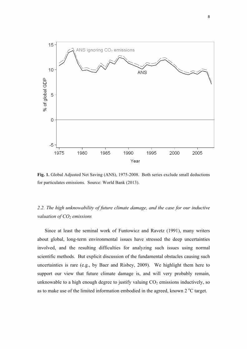
respectively. The World Bank then chose an SCC of $24.5/tC, based on Fankhauser

(1994), which values CO2 emissions during 1975-2008 at 0.4-0.5% of global gross

domestic product (GDP). This small value appears in Fig. 1 as the narrow gap

between the two graphs for global ANS during this period, which ignore or include

the CO2 deduction. As noted below in Section 4.1, $24.5/tC is close to DICE’s

optimal SCC and is a key reason for our choosing DICE. It is thus also consistent

with DICE’s associated, non-optimal scenario, where warming reaches 6.1 oC if

emissions remain uncontrolled for 250 years, yet average well-being, our term for

Nordhaus’s (2008: 39) “generalized consumption per person”, still grows 19-fold, to

only ~10% less than the hypothetical 21-fold growth that would occur without the

resulting climate damage.

Such minimal projected damage to well-being is in stark contrast to increasingly

strong warnings by climate scientists about dangerous global warming (e.g., Hansen

et al., 2008, 2012; Smith et al., 2009), and also to the importance of CO2 suggested by

the pessimistic, “strong sustainability” indicators in Fig. 2. These show the trends of

global Ecological Reserve – defined as [Biocapacity minus Ecological Footprint]

divided by Biocapacity, and also known as “ecological overshoot” when negative –

ignoring or including deductions for CO2 emissions (the Carbon Footprint). The

popular and influential Ecological Footprint adds up “the area required to produce the

resources people consume [and] the area occupied by infrastructure” (WWF, 2012),

so Ecological Reserve does not claim to be a society-wide sustainability indicator, and

is not quantitatively comparable with ANS. Nevertheless, both indicators claim to

indicate unsustainability when negative, so they are comparable in terms of sign and

trend, and to that extent they disagree strongly. We next consider in detail the

difficulty in resolving scientifically such deep disagreements about the importance of

CO2 to sustainability.

8

Fig. 1. Global Adjusted Net Saving (ANS), 1975-2008. Both series exclude small deductions

for particulates emissions. Source: World Bank (2013).

2.2. The high unknowability of future climate damage, and the case for our inductive

valuation of CO2 emissions

Since at least the seminal work of Funtowicz and Ravetz (1991), many writers

about global, long-term environmental issues have stressed the deep uncertainties

involved, and the resulting difficulties for analyzing such issues using normal

scientific methods. But explicit discussion of the fundamental obstacles causing such

uncertainties is rare (e.g., by Baer and Risbey, 2009). We highlight them here to

support our view that future climate damage is, and will very probably remain,

unknowable to a high enough degree to justify valuing CO2 emissions inductively, so

as to make use of the limited information embodied in the agreed, known 2 oC target.

9

Fig. 2. Global Ecological Footprint data shown as Ecological Reserve, 1975-2008. Source:

Global Footprint Network (www.footprintnetwork.org).

Because the Earth is unique in its complex geophysical and biological systems,

controlled global experiments are impossible. Comparisons with Venus’s greenhouse

effect, palaeoclimatic studies, and natural experiments like volcanic eruptions, can all

provide important insights into the Earth’s climate system, but cannot definitively

constrain its future behaviour. Humanity’s disturbances to the Earth’s systems

continue at unprecedented levels (Steffen et al., 2004), and their final effects will not

be known for centuries, if only because of the thermal inertia of oceans and ice-sheets

(Lenton et al., 2008; Richardson et al., 2011). Modelling future physical changes in

climate thus strains normal scientific methods to the limit; but estimating future

climate damage also needs to gauge the interaction of physical changes with an

unprecedented human population. History is of limited use: the growing evidence of

severe impacts of climate change on past societies (e.g., McMichael, 2012) cannot

yield a monetary estimate of future climate damage in a globalized economy with 8 or

9 billion people. Thus uniqueness, complexity, centuries-long time delays and the

10

human dimension combine to generate severe, scientifically unresolvable (non-

falsifiable) disagreements about estimating future climate damage, which are very

unlikely to be much reduced by learning over coming decades.

Our specific focus here is on disagreements about the damage function, defined

here as the proportion ω of global economic output lost by contemporaneous global

warming of T oC above the pre-industrial global temperature, or its complement, the

net-of-damage function Ω(T). A common formula, used here, is

ω(T) := 1 – Ω(T) = aTN / (1 + aTN); a, N > 0. (1)

There are many disagreements about other climate parameters, notably climate

sensitivity (the equilibrium global warming caused by doubling greenhouse gas

concentration, e.g., Weitzman, 2009, 2012), and growing criticisms of the assumption

in (1) that damage depends only on contemporaneous warming (e.g., Stern, 2013; Cai

et al., 2013). However, disagreements about ω(T) form our main reason for using

induction.

Conventional IAMs, including that in Stern (2007), use optimistic ω(T)’s,

estimated for a given warming (typically 2.5 and 3 oC) and then extrapolated, often

using an assumed quadratic form, to much higher temperatures (Tol, 2009; Aldy et al.,

2010). This yields direct disagreement with more pessimistic ω(T)’s at “super-

extreme” and “extreme” warming (say T ≈ 12 and T ≈ 6). For example, DICE’s

ω(T) = 0.0028388T2 / (1 + 0.0028388T2) (2)

(Nordhaus, 2007) has ω(12) = 29% and ω(6) = 9%, whereas Weitzman (2012) has

ω(12) = 99% and ω(6) = 50%. Disagreement among economists about ω(T) at

merely “high” warming (say T ≈ 3) is less marked. Nevertheless, most non-economist

supporters of a 2 oC warming limit still regard 3 oC as very dangerous; yet DICE’s

ω(3) is only 2.5%, close to the best-fit values estimated in Tol’s (2009, 2012) meta-

analyses of 13 other models, and equal to only around one lost year of consumption

growth.

11

Can elicitation of expert judgment settle such disputes? Expert elicitation is often

used to make subjective estimates of probabilities of future outcomes in climate

science, for example by Lenton et al. (2008) and Kriegler et al. (2009) for a range of

climate tipping points; but its only application to climate damage was by Nordhaus

(1994).3 His results were used for calculating DICE’s expected value of climate

catastrophe, and for example by Mastrandrea and Schneider (2004) to construct a

damage probability distribution. His study had only 19 participants from three high-

income countries and has not been repeated, so it would need updating and improving

– and would still face the fundamental obstacles already noted – if expert elicitation is

to play any future role in climate damage estimation.

Given this lack of data, all IAMs so far have had to use guesswork as the basis for

damage functions at higher temperatures. Dietz et al.’s (2007: 314-5) parameters for

both non-catastrophic and catastrophic climate damage were “essentially assumed” or

“genuine guesstimates”. Ackerman et al. (2010) used ω(T) = .0028388TN /

(1+.0028388TN) with N ranging stochastically from 1 to 5, but they called this choice,

and DICE’s N = 2 in (2), “arbitrary” and “fact-free” because “there is essentially no

relevant empirical research” (p. 1662). Similar language occurs in Dietz (2011: 523),

Weitzman (2012: 234) and Dietz and Asheim (2012: 328), and supports a stronger

criticism that directly estimated IAM damage functions “are completely made up,

with no theoretical or empirical foundation” (Pindyck, 2013: 870). The problem is

unavoidable, though not explicitly discussed, even in the most sophisticated recent

probabilistic models, for example Cai et al. (2013), who show the large effect on

SCCs of both risk aversion and irreversible shocks in climate damage. For although

probabilistic IAMs typically include uncertainty in the damage function, they still face

the high unknowability of the function’s probability distribution. We conclude that

estimating a precautionary valuation of CO2 by backwards, deterministic induction

from a globally agreed warming limit like 2oC is not in principle any less coherent or

more contentious than direct, probabilistic valuations which cannot avoid using rather

3 Weitzman (2012) cited Kriegler et al.’s expert elicitation of probabilities for climate tipping points as

rough evidence for his choice of ω(6), but such evidence that ω(6) = 50% instead of, say, 30% or 70%,

is very indirect.

12

arbitrary guesswork for key parameters, and is worth exploring as an alternative way

of dealing with underlying non-falsifiability. Using a CO2 valuation induced from a

“strong” warming limit might also give our modified ANS indicator more credibility

with some sustainability pessimists and environmental policy-makers.

Such induction can, however, use many different methods and/or models. In

particular, some readers may find implausible our assumption that a 2 oC warming

limit is optimal under standard discount rates. Many IAMs have instead assumed

higher intergenerational concern than implied by standard discounting, for example as

lower discount rates in Stern (2007), or as an ethical constraint like Dietz and

Asheim’s (2012) Sustainable Discounted Utilitarianism. An alternative would thus be

to vary such concern, but not DICE’s damage function, inductively to find what

makes a given warming limit optimal. As noted earlier, this alternative deserves

further research, but here we focus on higher climate damage and keep the World

Bank’s practice of using market prices, including discount rates, where possible.

A complementary alternative, also deserving further research, would be to use

induction in recent, probabilistic IAMs like Dietz and Asheim (2012) and Cai et al.

(2013).4 This could include risk aversion directly, rather than indirectly by our

precautionary recalibration of standard, deterministic DICE, and these models’ results

can depart significantly from deterministic models’. But such complex models are at

the frontiers of what is computationally possible, so adding induction would make

tractability challenging. Our use of a simpler, deterministic model allows a sharper

focus on why and how we use induction to tackle the high unknowability of climate

damage.

Irrespective of whether alternative, precautionary CO2 valuations are found

directly or inductively, using them to replace the existing valuation in World Bank

ANS raises further questions about our methodology, addressed at the end of the next

subsection. 4 Also Howarth et al (2014), if its saving and emissions control rates are endogenized so that optimal

control paths can be found.

13

3. Theory and practice of Adjusted Net Saving (ANS)

3.1. Theory

As currently estimated by the World Bank (2011, 2013), ANS for a geographical

region is:

basic ANS = KP !!!! .:...2211 =+++ jj KPKPKP , (3)

usually reported as a percentage of output, to make results comparable across time

and regions. Here K!!!! :),...,,( 21 =jKKK are the region’s net investments (rates of

change over time t, with iK! ≡ dKi / dt) in j stocks of manufactured, human,

knowledge, and foreign capital, and of environmental resources (also known as

natural capital), whose use affects the possibilities for human well-being.

P:),...,,( 21 =jPPP are rental prices, which measure the social benefits (discounted

dollar values over the rest of time, some of them negative, i.e. costs) of unit net

investments now in each stock; and the assumption of smooth substitutability, no

matter how limited, means that all prices are in principle finite. So K includes both

economic (owned) stocks like manufactured capital and fossil fuels, where rental

prices Pi can be estimated from market prices; and environmental (unowned) stocks

like CO2, where shadow rental prices must be estimated by environmental economists,

with difficulties in estimating Pi for CO2 already discussed above.

By allowing for exogenous population growth and technical progress, subject to

many restrictive conditions, Pezzey (2004) proved a one-sided theoretical link

between an extended form of ANS and sustainability in an “optimal” economy: one

which maximizes welfare W{L(t)u(t)} over the entire future, where L(t) is population

and u(t) is well-being (utility) per person. If n is the (constant) rate of population

growth, x(t) is the per-person benefit of future, exogenous technical progress that

results just from time passing, * denotes optimal values, and um(K(t)) is the maximum

utility sustainable forever starting from capital stocks K(t), the link is that:

14

extended ANS : )()( )(*).( )(*).( txtLttntt +−= KPKP ! ≤ 0

basic deduction for addition for ANS exogenous exogenous population growth technical progress

⇒ u*(t) > um(K*(t)) (4)

current utility > maximum sustainable utility; i.e., economy is unsustainable at t.

(See Appendix A for details.) However, current, extended ANS being positive does

not mean current well-being is sustainable. The intuition for this one-sidedness is that

optimality entails no concern for sustainability as defined here. Indeed, optimality

may directly cause an unsustained development path if non-renewable resource

depletion is essential for an economy (Dasgupta and Heal, 1974; Pezzey and

Withagen, 1998); and high optimal resource depletion rates, iK! , can drive optimal

rental prices iP (estimated from observed market prices) far below their “sustainability

prices” (Pezzey and Toman, 2002).

Among the key restrictions needed for (4) to hold (again see Appendix A) are that

n is exogenous and constant, as just noted; u depends only on per-person levels, C/L,

of an extended consumption vector C; and the economy’s production possibilities

have constant returns to scale. All these restrictions are inevitably broken by real-

world conditions. The population growth rate “is not and cannot be” forever constant

in practice (Arrow et al., 2003).5 The effect of any public, environmental good in C

on individual well-being u is not diluted by growth in population L. Globally

important environmental resources do not exhibit constant returns to scale, because

5 We find later that in our modified DICE, average well-being falls far below its optimal path when emissions are uncontrolled, so one might expect this to affect population. However, underlying growth in productivity means that well-being stays forever above its initial, 2005 level even on the uncontrolled path, thus giving no reason to suppose that starvation would check population growth. So it is unclear if uncontrolled emissions would lower, or raise, population in a more detailed model with endogenous population.

15

the global environment cannot be replicated.6 Nevertheless, (4) is the only known

theoretical connection between extended ANS and our sustainability definition.7 The

population term nP.K in (4) is the “Malthusian term” already calculated in World

Bank (2006, Appendix 4; 2011, Appendix E) for selected countries, but not connected

directly to sustainability or added up globally. There is no good, practical alternative

to the World Bank’s calculation method, reviewed in Section 4.3 below. That

subsection and Appendix B also explain how we calculated the technical progress

term x. Lx was once estimated to add about 40 percentage points of output to US

ANS (Weitzman, 1997), a large result which motivates its inclusion here.

Further questions, more specific to this paper’s methodology, arise from our

insertion below into World Bank ANS of the two very different SCCs derived from

optimal and no-control runs of our modified DICE. All observed prices and quantities

used in World Bank ANS come from economies that are essentially uncontrolled with

regard to the global natural environment. So our result that the no-control SCC is far

greater than the optimal SCC means that some optimal (non-CO2) prices and

quantities must be rather different from observed prices and quantities, which reduces

the accuracy of our estimate of optimal ANS. As for uncontrolled ANS, this has no

formal theoretical link with sustainability, given the optimality needed for (4) to hold,

so it can be regarded as only a heuristic indicator of global sustainability. But there is

no alternative sustainability theory available to avoid these shortcomings, which are

quite unrelated to our use of induction, and would arise from using SCCs from any

other IAMs with widely different optimal and no-control SCCs.

6 Also, constant returns to scale requires that one can assign meaning to a zero capital stock for each Ki,

which is effectively impossible for knowledge and environmental stocks. We thank a referee for noting

this, and the previous point on population endogeneity.

7 Both Arrow et al. (2003) and Asheim (2004) gave formulae for extended ANS when the population

growth is not constant, but both omitted the non-autonomous case and gave no connection to

sustainability as defined here.

16

3.2. World Bank practice

The World Bank uses no formal, explicit definition of sustainability, but seems to

use the definition in (4), judging by the following: “The rule for interpreting ANS is

simple: if ANS is negative, then we are running down our capital stocks and future

well-being will suffer; if ANS is positive, then we are adding to wealth and future

well-being” (World Bank 2011: 19). This statement overlooks the one-sidedness of

result (4). It also overlooks the fact that if wealth is viewed as P.K, the value of an

economy’s entire stocks, then the change in wealth over time is KPKP .. !! + , that is,

ANS, KP !. , plus the capital gains KP.! resulting from real price changes P! . But

despite these oversights, the Bank’s sustainability motivation for measuring ANS is

clear.

Table 1 lists the World Bank’s basic global ANS components in 2005, our year of

calculation for data reasons to be given in Section 4.3. Aggregation over countries

uses market exchange rates (with no equity weightings), but using purchasing-power-

parity rates makes little difference. The World Bank reports ANS as a percentage of

global gross national income, which differs from global GDP, our measure of output,

by only minor statistical errors. The 9.3% ANS result in Table 1 is little publicized,

but it suggests no general concern for future global well-being, despite the overall

ANS decline since 1975 shown in Fig. 1.

The omissions here of population growth and technical progress are addressed

below in Section 4.3. Practical difficulties in measuring many components in Table 1

are discussed by the World Bank (2011: 21-23); the Bank’s results are frequently

revised; and some important global environmental threats like biodiversity loss and

nitrogen pollution are extremely hard to value and therefore omitted.

17

Table 1. World Bank (2013) global Adjusted Net Saving (ANS) components in 2005

Components, },...,{ 11 jj KPKP !! Size (as % of

global GDP)

Net saving (gross saving, assumed to be invested in manufactured capital, minus depreciation of that capital)

8.7%

Public education spending (a proxy for investment in human capital) 4.3%

Market valuations of:

Depletion of fossil-fuel energy

Depletions of 10 minerals including phosphate

Net forest depletion

–2.9%

–0.2%

–0.0%

Non-market valuations of:

Human health damages from particulates emissions

Discounted long-term economic losses from climate change caused by current anthropogenic CO2 emissions

–0.2%

–0.4%

Total basic ANS ).( KP ! 9.3%

3.3. Another approach

Another approach to empirical sustainability measurement has been developed

from theory originated by Dasgupta and Mäler (2000), with notable recent

contributions being Arrow et al. (2012) and UNU-IHDP and UNEP (2012). This

approach appears to measure sustainability in non-optimal economies, and thus avoid

our problem of using a sustainability theory that applies only to optimal economies.

But it actually offers no advantage for our purposes, because it generally defines an

economy’s sustainability at t quite differently, as instantaneously non-declining

welfare ( 0)( ≥tW! at t).8 The approach then shows how 0)( ≥tW! at t can translate in

non-optimal economies into comprehensive wealth, measured at constant real prices,

being non-declining at t; or into variants of ANS, called comprehensive investment in

Arrow et al. and inclusive investment in UNU-IHDP, being non-negative at t. So

8 The original definition of sustainable development in Dasgupta and Mäler (2000: 83), though, was

non-instantaneous: “...from now, utility must never decline”.

18

while many details of comprehensive investment calculations in the Dasgupta-based

literature differ from the World Bank’s ANS calculations − in particular, Arrow et al.

found huge values for health capital, which we do not include here − the theoretical

link that one can then make with sustainability as defined in (4) is no different. Both

approaches also face the same problems of finding the shadow prices needed to

estimate ANS (Smulders, 2012).

4. Our modifications to DICE and to ANS

4.1. Choosing the DICE-2007 model for modification

Fankhauser’s (1994) method of valuing CO2 emissions, as used in World Bank

ANS, was designed for small-scale emission control projects, and cannot calculate

SCCs under optimal or no emissions control, or corresponding values of technical

progress. Our requirement in (4) for all these values led us to modify DICE-2007

(Nordhaus, 2008), one of the DICE/RICE series of IAMs including RICE-2010

(Nordhaus, 2010, where R = Regional), DICE-2010, and DICE-2013 (Nordhaus,

2013). Each model assumes global welfare maximization, with or without control of

industrial CO2 emissions, and includes exogenous technical progress. So each can

yield all our required values, in contrast to literature-based CO2 valuations (e.g., Tol,

2009), or to most other IAMs.9 The relative simplicity and generally good

documentation of DICE/RICE models further make them a suitable choice for our

inductive method. DICE-2007 is the most suitable, since RICE contains regional

detail irrelevant to our global analysis, and neither DICE-2010 nor DICE-2013 was

fully documented at the time of submission.10

DICE-2007’s SCC is close enough to cause no loss of accuracy when we use it in

place of the World Bank’s SCC in our estimates of ANS based on standard DICE.

9 WITCH (Bosetti et al., 2006 and subsequent papers) might be developed to yield the values needed

for our approach, but far less readily than DICE.

10 DICE-2013’s latest (October 2013) damage function is very close to DICE-2007’s.

19

Normalized to US2005$, SCC is $24.5/tC in World Bank (2011: 78); and $27.3/tC in

2005 in DICE-2007’s optimal run (Nordhaus, 2008: 92), where optimality would

require all policy-makers to create a uniform carbon price close to this SCC, using an

emissions tax or trading scheme with 100% participation (i.e., covering all global

emissions). SCC is $28.9/tC in 2010 in RICE-2010’s optimal run, so using RICE

would change little here. Reasons for not using recent, probabilistic variants of DICE

were given in Section 2.2.

4.2. Modifying DICE inductively to revalue CO2 emissions

For reasons already discussed, we derive a precautionary SCC inductively, by

modifying DICE so it becomes economically optimal for the world to be likely to stay

within an agreed warming limit. We choose the well-known 2 oC limit, and “likely”

means “with about 70% probability” – near the bottom of the 66-90% range for

“likely” used by IPCC (2007) – which allows us to use a result from probabilistic

climate science to calibrate our deterministic method. Like most IAM literature, we

omit a detailed description of DICE, which is documented in Nordhaus (2008), with

its computer code available in Nordhaus (2013). For reasons given earlier, we use

DICE’s “descriptive”, market values for discount rate parameters rather than any

“prescriptive”, ethical values as in Stern (2007). We make a likely, 2 oC warming

limit optimal by changing three DICE elements: the climate damage function, ω(T);

the path of non-CO2 radiative forcing over time t, labelled FEX(t); and the climate

(temperature) sensitivity parameter, labelled χ; see Appendix C for the code used.

The relationship among these three changes needs explanation. First, we do not

just impose an exogenous 2 oC warming constraint as in Nordhaus (2008), because 2 oC is too low to be optimal if DICE’s modest damage function in (2) is valid. Next,

we judge it insufficiently precautionary to modify only DICE’s damage function,

because of results in column (b) of Table 2. There we assume a temperature exponent

N = 5 (the highest value considered by Ackerman et al., 2010, though Dietz and

Asheim, 2012 considered N = 7) to give a damage curve with a steep threshold that

embodies a precautionary approach to tipping elements in the climate system (Lenton

20

et al., 2008; Richardson et al., 2011). We then find by induction that a = 0.00072

would make 2 oC maximum warming optimal, but would result in 1400 GtCO2

cumulative CO2 emissions during 2000-50. In a much-cited climate model

(Meinshausen et al., 2009), such emissions are equivalent to only a ~55% chance of

achieving a 2 oC maximum under uncertainty, which we consider not “likely” enough

for risk-averse policy-makers.

Table 2. Our modifications to standard DICE assumptions and results

(a) Standard DICE (b) DICE with steeper

damage as the only

change in parameters

(c) Our base-

case modified

DICE

Model parameters:

Parameters in climate damage

function (proportion of global

GDP lost),

ω(T) = aTN / (1+ aTN) (1)

N 2 5 5

a 0.0028388 0.00072† 0.00082†

Non-CO2 net radiative forcing, FEX(t)

(t = (year–2005)/10)

0.36 × [min(t/10,1)]

– 0.06

(Wm–2)

0.36 × [min(t/10,1)]

– 0.06

(Wm–2)

0.25

× [min(t/10,1)]

× CO2 forcing

Climate sensitivity, χ (oC) 3 3 4

Model results:

Maximum global warming T if CO2

emissions are optimal (oC)

3.5 2.0† 2.0†

Cumulative, optimally controlled

CO2 emissions, 2000-50 (GtCO2)

1670 1400 1110

† In our modifications, maximum, global warming is an exogenous assumption, and parameter a is

induced so that this maximum is economically optimal.

We therefore make two extra changes, each supported by recent climate science,

to lower the cumulative emissions that our modified DICE calculates as being

21

compatible with any given maximum warming. We thus arrive at a precautionary

recalibration of DICE, with a deterministic form of higher risk aversion (by achieving

the equivalent of a ~70% chance of 2 oC maximum warming), as well as a higher

climate damage function.

One extra change is to non-CO2 net radiative forcing. DICE’s FEX(t), which is

not separately documented in Nordhaus (2007), is independent of the CO2 emissions

path and results in non-CO2 forcing peaking at only 6-7% of CO2 forcing in 2105. By

contrast, IPCC (2007, Table 5.1) estimated that at stabilization, CO2-equivalent

concentrations (including non-CO2 gases), closely reflecting overall radiative forcing,

would over a wide range be at least 25% above CO2-only concentrations. Our base-

case modified DICE, defined by column (c) of Table 2, matches this by assuming

FEX(t) starts at zero in 2005, as in IPCC (2007), and rises to 25% of CO2 forcing in

2105 and thereafter. Higher, uncontrolled CO2 concentrations will thus be associated

with higher non-CO2 forcing, rather than unchanged non-CO2 forcing as less plausibly

assumed in DICE. Our non-CO2 forcing turns out to be higher overall in the

optimally controlled case as well (Fig. 3).

Fig. 3. Non-CO2 net radiative forcing in standard DICE and our modified DICE

22

Our last change is to raise climate sensitivity χ from 3 to 4 oC, which Sherwood

et al. (2014: 40) concluded is the “most likely” value. We then find by induction, still

assuming N = 5, that our changes to FEX(t) and χ together change the damage function

to ω(T) = .00082T5 / (1+.00082T5) and lower the 2000-50 emissions consistent with 2 oC maximum warming down to ~1100 GtCO2, as shown in column (c). Such

cumulative emissions raise the chance in Meinshausen et al. of achieving a 2 oC limit

to ~70%, as required. In keeping with our interpretation that the 2 oC (or any similar)

warming limit primarily reflects a policy of protecting future generations from climate

damage, rather than encouraging higher general intergenerational concern, this

function is much higher than DICE’s and other notable recent damage functions (Fig.

4), and shows a strong threshold effect over a 3−5 oC warming range.

Fig. 4. Global warming damage functions, ω(T). Our modified DICE function is compared

to those of Weitzman (2012), standard DICE (Nordhaus, 2007), and Stern (2007).

23

4.3. Adjustments to ANS for population growth and exogenous technical progress

We estimate that KP.n , the population deduction in (4), was 4.6% of global GDP

in 2005, as follows:

Growth rate of global population in 2005, n = 1.19 %/yr (World Bank, 2013).

Tangible wealth per person, P(2005).K(2005)/L(2005) = 27.12 k$/person

(World Bank, 2011: 181)

GDP per person in 2005 = 7.06 k$/person.yr (World Bank, 2013)

1.19% x 27.12 / 7.06 = 4.6%.

For reasons of data availability, the World Bank’s estimates of tangible wealth,

)().( tt KP , are based on a different set of stocks, K, than used for their basic ANS,

)().( tt KP ! (World Bank, 2011, Appendices D-E). Human capital and environmental

resource stocks, respectively changed by cumulative education expenditures and

cumulative emissions, are excluded from tangible wealth, both for data reasons, and

with an environmental stock like CO2 concentration because its effect per person is

undiluted by population growth. Data on tangible wealth are available only for 1995,

2000, and 2005, which finally explains our choice of 2005 as our year of modified

ANS calculations. As discussed in Section 3.1, any difference in non-CO2 prices and

quantities between paths with controlled and uncontrolled CO2 emissions is ignored

here, and deserves future research.

The lack of appropriate data on overall technical progress makes estimating its

current discounted value, x in (4), infeasible for many individual countries, but we can

estimate a global x from DICE’s assumed growth in total factor productivity, as

described in Appendix B. Since x depends on not just exogenously growing total

factor productivity, but also endogenous changes to manufactured capital resulting

from past investment and depreciation, we can and do compute different values for x

on paths with controlled and uncontrolled emissions, unlike with the cost of

population growth.

24

The number we finally add to ANS is not Lx/GDP, the percentage value of gross

technical progress. World Bank ANS already includes public education spending (a

rough estimate of total education spending), estimated at 4.3% of global GDP in 2005,

as a reclassification of spending from consumption to investment in human capital

(Table 1). Since human capital growth through education, a cause of total factor

productivity growth (Solow, 1957), is not included in DICE’s manufactured capital, it

must be already included in DICE’s productivity growth. Including both education

spending and all Lx/GDP in ANS would therefore be double-counting, so the

technical progress values reported below are for (Lx/GDP – 4.3%).

5. Results and sensitivity testing

5.1. Results

Because of its modest damage function, standard DICE’s economic results and

their application to ANS in Table 3 show very little difference between a future with

optimal control of industrial CO2 emissions, where maximum global warming is 3.5 oC, and a future with no control, where maximum warming is 6.1 oC. By contrast,

emissions control matters hugely in our modified DICE model, because of our

changes in Table 2 that make a likely, 2 oC warming limit optimal.

If industrial emissions are controlled to respect this limit, then our base-case

results in Table 3 value the current ANS emissions deduction at 2% of global GDP,

about 4 times higher than the World Bank’s, but we also add 16% of GDP for future

technical progress. Our modified ANS is then 19%, markedly more reassuring about

the sustainability of current, global well-being than the World Bank’s 9% in Table 1,

mainly because of the included benefit of technical progress, which on an optimal

path far outweighs the cost of population growth and our higher valuation of

emissions. Consistent with this, average well-being in 2105 is projected to be only

4% below the standard DICE level (Fig. 5a), despite the extra cost of much faster CO2

abatement.

25

Table 3. Global climatic and economic results using standard DICE and our modified DICE

over 2105-2595. Cases (a) and (c) are as in Table 2, whose case (b) is irrelevant here.

(a)

Stan-

dard

DICE

(c) Our

base-case

modified

DICE

Optimal control of industrial

CO2 emissions

Maximum global warming (oC) 3.5 2.0

Social cost of CO2 emissions (SCC)

in 2005

($/tC) 27 131

(% GDP) –0.5 –2.2

#Value of technical progress, as at 2005 (% GDP) 15.7 16.0

##Adjusted Net Saving (ANS) in 2005 (% GDP) 20.5 19.0

No control of industrial CO2

emissions

Maximum global warming (oC) 6.1 6.0

SCC in 2005 ($/tC) 28 1455

(% GDP) –0.5 –24.4

#Value of technical progress, as at 2005 (% GDP) 15.6 7.2

##ANS in 2005 (% GDP) 20.3 –12.0

Decade of peak well-being in DICE None 2065

#Net of 4.3% educational spending (see end of Section 4).

##Sum of CO2 emissions and technical progress as shown here, plus 5.2% GDP for sum of net saving

(8.7%), public education spending (4.3%), natural resource depletion (–3.1%) and particulates pollution

(–0.2%) from Table 1, and of population growth (–4.6%) from Section 4.3.

But with no CO2 control, warming is much faster, so each ton of current emissions

causes much more future damage. This raises our deduction for current emissions

another 11-fold, from 2% to 24% of global GDP; and owing to depressed future

investment (Appendix B, Fig. 5b), it also lowers the sustainability value of technical

progress to only 7%. Our modified ANS in 2005 is then –12% of GDP (Table 3).

26

a

b Fig. 5. Average well-being (a) and gross investment per person (b) in our base-case modified

DICE, on different vertical scales. (Standard DICE graphs for No CO2 control are omitted

because on them, well-being and investment are only 0.7% and 1.4% below Optimal in 2105.)

Average human well-being is higher for the first two decades (Fig. 5a), but then

grows more slowly and peaks in 2065, because climate damage eventually exceeds

the benefits from capital investment and technical progress. Given the absence of any

theory-based alternative, this suggests that negative ANS may serve as a heuristic

indicator of the unsustainability of an uncontrolled, business-as-usual development

27

path. So on the basis of just Table 3’s results, our provisional answer to both our

opening questions would be ‘yes’: with optimal environmental management, current

well-being is found to be sustainable, even with a “strong” limit on global warming;

but with uncontrolled environmental damage, the future rise in well-being is

unsustainable. Together these results would challenge the beliefs of both

environmental pessimists and environmental optimists, and we can but hope such

challenges would inspire some more nuanced debate between supporters of the two

paradigms. But given the many contentious assumptions on which our results rest,

they first need to be tested, as follows.

5.2. Sensitivity testing

DICE contains 44 non-trivial parameters (Nordhaus, 2008: 58). Anderson et al.

(2014) used Monte Carlo simulations to perform a probabilistic, global sensitivity

analysis on DICE, whereby all its parameters are varied simultaneously, with each

assigned a uniform distribution from 10% below to 10% above its base value, and

with all base values given equal standing. In contrast to standard, one-factor-at-a-time

analyses, this allows for interactions among parameters, and avoids prejudging which

parameters are worth selecting for analysis. However, the unavoidable uncertainty

about what parameters to include in an IAM in the first place remains (Dietz and

Fankhauser, 2010). Also, using a uniform, non-judgmental approach to testing values

for included parameters can discard some useful knowledge. For example, some base

values for parameters can be calibrated quite well against current observations, and

are thus more reliably known than others; and credible ranges of variability may be

much wider for some parameters than for others. So while a global sensitivity

analysis would undoubtedly be desirable, a good one is necessarily complex, and we

leave these complexities to future research. Instead we have used our judgment to

choose parameters that define the eight, one-factor-at-a-time tests shown in columns

(d)-(k) of Table 4, which are ranked in descending order of impact on no-control ANS

compared to our base case in column (c).

28

Table 1. Sensitivity tests of our modified DICE model results. Case (c) is as in Table 2. Notes on technical progress and ANS results are as in Table 3.

(c) Base case of our mod-ified DICE

(d) Higher warming limit: 2.2 not 2.0 oC

(e) Lower climate sensitivity: χ = 3.6 not 4 oC

(f) Higher capital elasticity of output: γ = 0.33 not 0.3

(g) Total factor product'y A always 10% lower

(h) Lower damage exponent: N = 4.5 not 5

(i) Lower part-icipation rate: 90% not 100%

(j) Lower cons-umption elasticity: α = 1.8 not 2

(k) Faster technical progress: GA0 = 0.101 not 0.092

Optimal control of industrial CO2 emissions

Social cost of CO2 emissions (SCC) in 2005

($/tC) 131 97 108 105 121 136 160 134 127

(% GDP) –2.2 –1.6 –1.8 −1.8 −2.0 –2.3 –2.7 −2.2 –2.1

Value of technical progress, as at 2005 (% GDP) 16.0 15.9 15.9 15.4 18.7 16.0 16.0 17.1 20.0

Adjusted Net Saving (ANS) in 2005

(% GDP) 19.0 19.4 19.3 18.8 21.9 18.9 18.4 20.0 23.1

Rank re (c)* – 5 6 7 2 8 4 3 1

No control of industrial CO2 emissions

SCC in 2005 ($/tC) 1455 801 901 929 1053 976 1872 1310 1460

(% GDP) –24.4 –13.4 –15.1 −15.6 −17.7 –16.4 –31.4 −22.0 –24.5

Value of technical progress, as at 2005 (% GDP) 7.2 8.6 8.3 8.0 9.8 8.2 6.6 7.7 10.1

ANS in 2005(% GDP) –12.0 0.4 −1.6 −2.4 −2.7 −2.9 –19.6 −9.1 –9.2

Rank re (c)* – 1 2 3 4 5 6 7 8

Decade of peak well-being in modified DICE 2065 2075 2075 2075 2075 2075 2065 2075 2065

* Ranked in descending order of % GDP change from no-control ANS in (c) (so No-control ANS is least sensitive to a 10% change in parameter (k), ranked 8).

29

Our choice was nevertheless mainly inspired by Anderson et al.’s method and

results. First, each of our eight parameters is changed by 10% from its base value in

our modified DICE, with the changes all chosen to improve no-control ANS, except

for the emissions-pricing participation rate (column (i)), which cannot be improved

from its initial level of 100%. Second, the five parameters which define columns (e)-

(h) and (j) are those with the most impact on optimal SCC in Anderson et al.’s analysis

(excluding a in Table 2, which we always determine inductively so that the warming

limit is still optimal). Two further parameters − the warming limit in (d), and the rate

of technical progress in (k) − were of obvious interest, given their role in our ANS

methodology. Our eighth parameter was the participation rate. We found ANS to be

quite sensitive to this, even though it was one of the least sensitive parameters in

Anderson et al.’s analysis which started from DICE’s standard values for the damage

parameters N and a. Moreover, a halved participation rate seems much more likely

and thus worth considering than, say, a doubled total factor productivity, which again

shows the limits of a strictly non-judgmental approach to sensitivity analysis.

Our tests all show large differences between optimal and no-control SCCs, and

between optimal and no-control ANSs. This is reassuring for our methodology, if

unsurprising given how much higher climate damage is in our modified DICE than in

conventional models. The smallest difference between optimal and no-control ANSs is

19 percentage points, in (d) where the warming limit is 2.2 oC. This higher limit nearly

halves the no-control SCC and causes the greatest change in no-control ANS from our

base case (c), making it just positive. However, Table 4’s last row shows that in (d),

peak well-being in modified DICE is delayed by only a decade, rather than avoided,

suggesting only a one-sided link between ANS and sustainability also in the no-control

case.

Despite no-control ANS being most sensitive in our tests to two climate-related

parameters (the warming limit in (d), followed by climate sensitivity in (e)), two

economic parameters (capital elasticity in (f) and total factor productivity in (g)) are

close behind, suggesting no particularly sharp focus on which parameters deserve top

priority in future research. Moreover, sensitivity depends on the policy question

30

considered to be of interest. The rank order of sensitivity of ANS is very different

between optimal control and no control, with some changes in ANS from base case (c)

even having opposite sign for optimal and no-control runs, as with cases (f) and (h).

The rank order of sensitivity is different again if SCC (CO2 control) rather than ANS

(global sustainability) is of interest. For example, a 10% change in the rate of technical

progress, (k), has the least effect on no-control ANS and the second-least effect on

controlled SCC, but the greatest effect on controlled ANS.

6. Can ANS use induction to include other global environmental concerns?

Here we consider if ANS might be further extended to include other major

environmental concerns for global sustainability, such as Rockstrom et al.’s (2009)

“planetary boundaries”. A full treatment would need another paper, and references

here are merely illustrative. Nevertheless, considering biodiversity loss, and

conversion of atmospheric nitrogen to reactive forms – judged by Rockstrom et al. to

be the two most exceeded planetary boundaries – together with food security, suggests

some potential for our inductive approach to make ANS yet more inclusive, but also

the great difficulties of doing so. More straightforward, non-inductive extensions

would also be possible, such as including intragenerational inequality via regional

disaggregation (e.g., after Nordhaus, 2010), endogenous technical change (e.g., after

Popp, 2004), or carbon-cycle feedback (as suggested by Hof et al., 2012).

Inclusion of any new environmental variable i in ANS requires an estimate of both

its current net stock change, iK! , and its current, discounted social value per unit, iP .

Such estimates for global biodiversity loss are conceivable by developing a loss model

like that in Braat and ten Brink (2008), which uses population, GDP, energy use, and

food production as drivers. A precautionary value might then be induced from an

exogenous, “strong sustainability” limit on biodiversity loss, similar to our induction of

a precautionary CO2 value. But unlike CO2 emissions, biodiversity is heterogeneous,

with Braat and ten Brink’s use of mean species abundance as its aggregate measure

contrasting with Rockstrom et al.’s use of total species number. As for atmospheric

31

nitrogen conversion, this flow is measurable, but as yet there is no global modeling of

its determinants. So including nitrogen in ANS, even inductively, is even further off.

Growing concern is also being expressed (e.g., by Godfray et al., 2010) about the

world’s future ability to feed its population, and hence about sustainability as defined

here since food is vital to well-being. But by contrast with biodiversity loss and

nitrogen pollution, food production and consumption are mainly marketed, hence

already represented, albeit imperfectly, in our modified ANS. For example, the World

Bank (2011) estimates of KP.n in (4) include market values for four categories of

rural and urban land (say P1K1,...,P4K4), and thus how population growth cuts food

supply per person ceteris paribus by cutting land available per person. However, net

changes in quality-adjusted land stocks, ),...,( 41 KK !! , are not available separately (World

Bank, 2011: 38) and so are excluded. By contrast, phosphate rock is included in

ANS’s mineral depletion term (Table 1), so its valuation there at much less than 0.2%

of global GDP lends no support to Cordell et al.’s (2009) grave concern about the

effect of future phosphorus depletion on global food security. Supporting this concern

within a modified ANS would require a calculation, perhaps using an extended IAM,

that the ultimate non-substitutability of phosphate fertilizer in food production implies

a sustainability price (Pezzey and Toman, 2002) vastly bigger than the market-based

rental price currently used in World Bank ANS.

7. Conclusions

More than two centuries after Malthus started the debate on the limits that finite

environmental resources and population growth impose on the long-term, sustainable

growth of human well-being, there is a persistent gulf between optimistic and

pessimistic views on such limits and the indicators supporting them. Economic

(“weak”) indicators like the World Bank’s Adjusted Net Savings (ANS) and physical

(“strong”) indicators like the Ecological Footprint suggest starkly different,

respectively optimistic and pessimistic, futures for the world, and in particular attach

vastly different importance to current CO2 emissions. The Earth’s uniqueness, and the

32

complexity and long time-scales of key global changes, mean that many limits of

substituting human-made for environmental inputs to well-being are, and will stay,

highly unknowable. Opposing views on global sustainability will thus tend to remain

beliefs or paradigms, whose disagreement cannot be resolved by normal scientific

methods.

To address this gulf and help inform policy-making on global sustainability issues,

we have constructed an experimental, more inclusive, hybrid (“weak/strong”) indicator

of global sustainability. We extended World Bank ANS to include two important

omitted features – the cost of exogenous population growth and benefit of exogenous

technical progress – and replaced the CO2 emissions valuation by either one of two,

much higher, precautionary valuations, which assume either optimally controlled or

uncontrolled future emissions. Because damage from future global warming is highly

unknowable, we calculated these valuations inductively: we modified the damage,

climate sensitivity, and non-CO2 forcing assumptions in the deterministic, DICE

integrated assessment model so that an emissions path likely to limit global warming to

2 oC (an agreed “strong sustainability” constraint which is known) becomes

economically optimal. And to focus on climate damage rather than general

intergenerational concern as the main driver of climate policy, we left discount rates

unchanged at market-based, policy-relevant values. However, such induction does not

make the cost of exceeding 2 oC warming infinite, as logically implied by the language

of (absolute) non-substitutability used in much “strong sustainability” writing.

If future CO2 emissions are optimally controlled, our base-case, modified ANS is

substantially higher than World Bank ANS, mainly thanks to including the benefit of

exogenous technical progress. Consistent with this, our modified-DICE model has

well-being growth very close to DICE’s original. But if emissions are uncontrolled,

our CO2 cost is much higher than the World Bank’s, (exogenous) technical progress is

less beneficial because (endogenous) future investment falls, and base-case ANS is

negative. Consistent with this, well-being in modified-DICE peaks in 2065,

contradicting the conventional economic expectation of limitless growth. This

suggests that a negative “uncontrolled ANS” – one using valuations based on a future

33

path of uncontrolled environmental damage – may be a useful, if heuristic, indicator of

the unsustainability of rising well-being on that path. Our results are sensitive to

changes in parameter values, but none of eight key parameters tested was much more

important than the others, though the warming limit used for induction, still deserves

special scrutiny. Also, which parameters are considered the most important depends

on the policy context of interest (climate policy or global sustainability, controlled or

uncontrolled scenarios).

Our highly provisional answers to our two opening questions would thus be that the

current level of well-being may be sustainable if the global economy and environment

are optimally controlled in future; but rising well-being may not be sustained for

another century or so if business-as-usual trends of largely uncontrolled environmental

depletion continue. Such results depend on unavoidably contentious assumptions, and

we regard our contribution here as being perhaps more our methodology than our base-

case results, though our results do show how carefully qualified optimistic and

pessimistic views on global sustainability can both be right. How well the global

environment will in fact be controlled is a separate issue, though, on which optimistic

or pessimistic views may be held independently.

Several topics remain for future research. An important but tough challenge would

be to use induction to include “planetary boundaries” for other global environmental

threats in ANS, like biodiversity loss and nitrogen pollution, which are also

unknowable enough to be near-impossible to value directly. An easier extension in

terms of data-gathering, but perhaps harder computationally, would be to use induction

in existing, probabilistic versions of DICE which explicitly model important aspects of

uncertainty (as opposed to unknowability) that our deterministic approach omits, like

policy-makers’ risk aversion. Adding carbon-cycle feedback, endogenous population

change, and endogenous technical progress would also be desirable. The ultimate aim

might be to extend such a model even further to include important sectors like energy

and minerals depletion, so the model could then be used to make direct predictions of

global sustainability, not just provide values for a hybrid ANS as here. However, a

separate, more complete model might actually have less influence on policy than a

34

further modification of World Bank ANS. The theoretical, data-gathering, and

modelling challenges of all such extensions are severe, so multiple, simpler

sustainability indicators will still be needed. But we hope our attempt to build a single,

more inclusive, economic indicator of global sustainability which incorporates both

technical progress and a physical, environmental constraint will be of interest to

policy-makers, and a useful addition to the mostly polarized debate between

environmental optimists and pessimists.

Acknowledgments

We thank two anonymous referees for their careful, detailed comments on earlier

drafts. We also thank Joern Fischer, Quentin Grafton, Kirk Hamilton, Nick Hanley, Rob

Heinsohn, Charles Jenkins, Duncan McIntyre, Mike Raupach, Will Steffen, Mike Toman,

and many others for a wealth of helpful comments. We thank the Australian

Government’s Commonwealth Environment Research Facilities program for financial

support. All errors and opinions are ours.

Appendix A. Further details of ANS theory

Pezzey’s (2004) theoretical link between extended ANS and sustainability in (4) is

summarized as follows. Society’s intertemporal welfare W(0) is the discounted present

value of average utility (well-being) per person weighted by population:

∫∞ −=0

)](/)([ )(: )0( dtetLtutLW tρC , (A.1)

and four key restrictive conditions for result (4) to hold are:

• C(t) is “extended consumption”, the vector of all attributes, including consumption of

goods and services and various measures of environmental quality, whose per-person

levels determine a representative agent’s instantaneous utility, u(C/L);

• L(t) = L0 ent is population, assumed to be growing exogenously at constant rate n;

• ρ > 0, the utility (pure time) discount rate is constant; and

35

• W(0) is maximized subject to ]),(),([)](),([ ttLtStt KKC ∈! at all times, where S[.],

the economy’s “extended production” possibility set, has constant returns to scale,

and is non-autonomous (depends directly on time t) to allow for exogenous technical

progress.

Term x(t) in (4), the per-person realized value of exogenous technical progress in

expanding production possibilities over time, is:

x (t) ∫ ∫∞

−−∂∂=

}])([ exp{ ]/)([:

t

s

tdsdznzrssy , (A.2)

where y(t) is (green) Net National Product per person and r(t) is the real interest rate at

time t (see Propositions 5 and 8 in Pezzey, 2004, which generalize and extend

Weitzman, 1997). Appendix B explains how we estimate x(t) empirically.

In addition to, or derived from, the four key conditions already noted, further

assumptions needed to make (4) true include that:

(i) all decision-makers have perfect information over an infinite time horizon, and

social planners use this to make the economy follow its optimal path over time;

(ii) the optimal time-path of utility is unique and non-constant;

(iii) all stocks affecting production and utility, K, and net investments in them, K! , are

measurable;

(iv) all such stocks have finite prices, P, which in turn assumes smooth

substitutability everywhere between human-made inputs and natural inputs to

production and utility;

(v) by measuring the welfare of just a representative agent, and discounting it over

all time, all decision-makers are ethically willing to aggregate dollar values over

all present and future people, and ignore all intranational, international, and

intergenerational inequalities in well-being;

(vi) there are no public goods or bads (since the effect of these on utility would not be

divided by population L as in (A.1), as noted in Pezzey 2004: 625); and

(vii) there are no renewable resource stocks with non-constant returns to scale.

36

Appendix B. Using DICE to estimate the ANS addition for technical progress

We estimate the per-person value x(0) of exogenous technical progress using this

discrete approximation of (A.2) applied to results from DICE runs:

x(t) ∑ ∑= =−−ΔΔ≈

18 })]()([10exp{]/)(~[ts

s

tzdsdzznzrssy , (B.1)

with t in decades as in DICE, but with r and n as annual rates, hence the required factor

of 10. This approximates y, green Net National Product per person, as y~ , per-person

output, net of climate damage ω and manufactured capital depreciation δK:

)(/)}()](1[)]([)]()[({:)(~ 1 sLsKTsLsKsAsy δωγγ −−= − (B.2)

where previously undefined terms in DICE are two variables: (exogenous) total factor

productivity A(t) and (endogenous) manufactured capital K(t); and two parameters: γ,

the capital elasticity of Cobb-Douglas gross output, and δ, the rate of capital

depreciation.

To compute Δ y~ (s)/Δs in (B.1), we start by computing annual growth rates of

population and technology for t = 0, ...,18 (i.e. from 2005-2185) as

n(t) = [L(t+1)/L(t)]1/10 – 1 and gA(t) := [A(t+1)/A(t)]1/10 – 1, respectively, (B.3)

so the growth rate in y~ (t) due solely to technical progress is

[Δ y~ (t)/Δt]/ y~ (t) = gA(t)–n(t), and Δ y~ (s)/Δs in (B.1) is [gA(s)–n(s)] y~ (s). (B.4)

Next, we compute the geometric, annual rate of interest

r(z) := [1+r10(z)]1/10 – 1, (B.5)

where r10(z) is the decadal interest rate computed by DICE.

We finally estimate x(0) from (B.1). This is much lower on the no-control path

than on the optimal path, because with no control, in anticipation of much higher

climate damage, investment falls rather than rises over time (Fig. 5b). This leads to

falling rather than rising capital, hence higher interest rates r and heavier discounting

in (B.1).

37

Appendix C. Our modifications to DICE’s computer code

Original lines of GAMS code for DICE-2007

T2XCO2 Equilibrium temp impact of CO2 doubling oC / 3 /

FEX0 Estimate of 2000 forcings of non-CO2 GHG / -.06 /

FEX1 Estimate of 2100 forcings of non-CO2 GHG / 0.30 /

A2 Damage quadratic term / 0.0028388 /

A3 Damage exponent / 2.00 /

FORCOTH(T) = FEX0 + .1*(FEX1-FEX0)*(ORD(T)-1)$(ORD(T)LT12) + 0.36$(ORD(T)GE12);

FORC(T) =E= FCO22X*((log((Matav(T)+.000001)/596.4)/log(2))) + FORCOTH(T);

*s.fx("1") = .22;

[The last line is from Nordhaus’s code, with * meaning that fixing the first-period

saving rate s at 22% should be suppressed. However, experimentation shows that to

get the exact results shown in Nordhaus (2008), the command s.fx("1")=.22; must not

be suppressed, so we make it operational in our modified DICE, as shown below.]

Replacement lines in our modified DICE (Table 2, column (c))

T2XCO2 Equilibrium temp impact of CO2 doubling oC / 4 /

A2 Damage quadratic term / 0.00082 /

A3 Damage exponent / 5.00 /

FORCOTHM(T) = 0.025*(ORD(T)-1)$(ORD(T)LT12) + 0.25$(ORD(T)GE12);

FORC(T) =E= FCO22X*((log((Matav(T)+.000001)/596.4)/log(2))) * FORCOTHM(T);

s.fx("1") = .22;

-oOo-

38

References

Ackerman, F., Stanton, E.A., Bueno, R., 2010. Fat tails, exponents, extreme uncertainty: Simulating catastrophe in DICE. Ecological Economics 69, 1657–1665.

Aldy, J.E., Krupnick, A.J., et al., 2010. Designing climate mitigation policy. Journal of Economic Literature 48, 903–934.

Anderson, B., Borgonovo, E., et al., 2014. Uncertainty in climate change modeling: Can global sensitivity analysis be of help? Risk Analysis 34, 271-293.

Arrow, K.J., Dasgupta, P., et al., 2012. Sustainability and the measure of wealth. Environment and Development Economics 17, 317–353.

Arrow, K.J., Dasgupta, P., Mäler, K.-G., 2003. The genuine savings criterion and the value of population. Economic Theory 21, 217–225.

Asheim, G.B., 2004. Green national accounting with a changing population. Economic Theory 23, 601–619.

Baer, P., Risbey, J.S., 2009. Uncertainty and assessment of the issues posed by urgent climate change. An editorial comment. Climatic Change 92, 31–36.

Bosetti, V., Carraro, C., et al., 2006. WITCH: A world induced technical change hybrid model. Energy Journal 27, 13–37.

Braat, L., ten Brink, P. (Eds.), 2008. The Cost of Policy Inaction: The Case of Not Meeting the 2010 Biodiversity Target. Alterra, Wageningen, Netherlands.

Brock, W.A., Taylor, M.S., 2010. The Green Solow model. Journal of Economic Growth 15, 127–153.

Cai, Y., Judd, K.L., Lontzek, T.S., 2013. The social cost of stochastic and irreversible climate change. NBER Working Paper 18704.

Cordell, D., Drangert, J.O., White, S., 2009. The story of phosphorus: Global food security and food for thought. Global Environmental Change 19, 292–305.

Dasgupta, P.S., Heal, G.M., 1974. The optimal depletion of exhaustible resources. Review of Economic Studies 41, 3–28.

Dasgupta, P.S., Mäler, K.-G., 2000. Net national product, wealth, and social well-being. Environment and Development Economics 5, 69–94.

Dietz, S., 2011. High impact, low probability? An empirical analysis of risk in the economics of climate change. Climatic Change 108, 519–541.

Dietz, S., Asheim, G.B., 2012. Climate policy under sustainable discounted utilitarianism. Journal of Environmental Economics and Management 63, 321–335.

Dietz, S., Fankhauser, S., 2010. Environmental prices, uncertainty, and learning. Oxford Review of Environmental Policy 26, 270–284.

Dietz, S., Hope, C., Patmore, N., 2007. Some economics of 'dangerous' climate change: Reflections on the Stern Review. Global Environmental Change 17, 311–325.

Dietz, S., Neumayer, E., 2007. Weak and strong sustainability in the SEEA: concepts and measurement. Ecological Economics 61, 617-626.

Fankhauser, S., 1994. The social costs of greenhouse gas emissions: an expected value approach. Energy Journal 15, 157–184.

39

Funtowicz, S.O., Ravetz, J.R., 1991. A new scientific methodology for global environmental issues. In: Costanza, R. (Ed.), Ecological Economics: The Science and Management of Sustainability, Columbia University Press, New York, NY, pp. 137–152.

Gagnon, N., Hall, C.A.S., Brinker, L., 2009. A preliminary investigation of Energy Return on Energy Investment for global oil and gas production. Energies 2, 490–503.

Gjerde, J., Grepperud, S., Kverndokk, S., 1999. Optimal climate policy under the risk of a catastrophe. Resource and Energy Economics 21, 289–317.

Godfray, H.C.J., Beddington, J.R., et al., 2010. Food security: the challenge of feeding 9 billion people. Science 327, 812–818.

Guivarch, C., Hallegatte, S., 2013. 2C or not 2C? Global Environmental Change 23, 179–192.

Hamilton, K., 1994. Green adjustments to GDP. Resources Policy 20, 155–168. Hamilton, K., Clemens, M., 1999. Genuine savings rates in developing countries. World Bank

Economic Review 13, 333–356.

Hansen, J., Sato, M., et al., 2008. Target atmospheric CO2: Where should humanity aim? Open Atmospheric Science Journal 2, 217–231.

Hansen, J., Sato, M., Ruedy, R., 2012. Perception of climate change. Proceedings of the National Academy of Sciences of the USA 109, E2415–E2423.

Hof, A.F., Hope, C.W., et al., 2012. The benefits of climate change mitigation in integrated assessment models: the role of the carbon cycle and climate component. Climatic Change 113, 897–917.

Howarth, R.B., Gerst, M.D., Borsuk, M.E., 2014. Risk mitigation and the social cost of carbon. Global Environmental Change 24, 123-131.

IPCC (Intergovernmental Panel on Climate Change), 2007. Climate Change 2007: Synthesis Report. IPCC, Geneva, Switzerland.

Krausmann, H., Erb, K.H., et al., 2013. Global human appropriation of net primary production doubled in the 20th century. Proceedings of the National Academy of Sciences 110, 10324–10329.

Kriegler, E., Hall, J.W., et al., 2009. Imprecise probability assessment of tipping points in the climate system. Proceedings of the National Academy of Sciences 106, 5041–5046.

Lenton, T.M., Held, H. et al., 2008. Tipping elements in the Earth’s climate system. Proceedings of the National Academy of Sciences 105, 1786–1793.

Mastrandrea, M.C., Schneider, S.H., 2004. Probabilistic integrated assessment of 'dangerous' climate change. Science 304, 571–575.

McMichael, A.J., 2012. Insights from past millennia into climatic impacts on human health and survival. Proceedings of the National Academy of Sciences 109, 4730–4737.

Meadows, D.H., Meadows, D.L., et al., 1972. The Limits to Growth. Universe Books, New York, NY.

Meinshausen, M., Meinshausen, N., et al., 2009. Greenhouse-gas emission targets for limiting global warming to 2 oC. Nature 458, 1158–1163.

Neumayer. E., 2013. Weak versus Strong Sustainability: Exploring the Limits of Two Opposing Paradigms, 4th edn. Edward Elgar, Cheltenham, UK.

Nordhaus, W.D., 1973. World Dynamics - measurement without data. Economic Journal 83, 1156–1183.

Nordhaus, W.D., 1994. Expert opinion on climatic change. American Scientist 82, 45–51.

40

Nordhaus, W., 2007. Accompanying Notes and Documentation on Development of DICE-2007 Model. http://people.anu.edu.au/jack.pezzey/Nordhaus2007DICEnotes.pdf.

Nordhaus, W., 2008. A Question of Balance. Yale University Press, New Haven, CT. Nordhaus, W.D., 2010. Economic aspects of global warming in a post-Copenhagen environment.

Proceedings of the National Academy of Sciences 107, 11721–11726. Nordhaus, W., 2013. DICE 2013: Introduction and User’s Manual, October.

www.econ.yale.edu/~nordhaus/homepage/.

Pezzey, J.C.V., 1997. Sustainability constraints versus 'optimality' versus intertemporal concern, and axioms versus data. Land Economics 73, 448–466.

Pezzey, J.C.V., 2004. One-sided sustainability tests with amenities, and changes in technology, trade and population. Journal of Environmental Economics and Management 48, 613–631.

Pezzey, J.C.V., Toman, M.A., 2002. Progress and problems in the economics of sustainability, in: Tietenberg, T., Folmer, H. (Eds.), International Yearbook of Environmental and Resource Economics 2002/3, Edward Elgar, Cheltenham, UK, pp. 165–232.

Pezzey, J.C.V., Withagen, C.A., 1998. The rise, fall and sustainability of capital-resource economies. Scandinavian Journal of Economics 100, 513–527.

Pindyck, R.S., 2013. Climate change policy: what do the models tell us? Journal of Economic Literature 51, 860–872.

Popp, D., 2004. ENTICE: endogenous technological change in the DICE model of global warming. Journal of Environmental Economics and Management 48, 742–768.

Richardson, K., Steffen, W., Liverman, D. (Eds.), 2011. Climate Change: Global Risks, Challenges and Decisions, Cambridge University Press, Cambridge, UK, pp. 163–201.

Rockstrom, J., Steffen, W., et al., 2009. A safe operating space for humanity. Nature 461, 472–475.

Sherwood, S.C., Bony, S., Dufresne, J.-L., 2014. Spread in model climate sensitivity traced to atmospheric convective mixing. Nature 505, 37–42.

Smith, J.B., Schneider, S.H., et al., 2009. Assessing dangerous climate change through an update of the Intergovernmental Panel on Climate Change (IPCC) ‘‘reasons for concern’’. Proceedings of the National Academy of Sciences 106, 4133–4137.

Smulders, S., 2012. An arrow in the Achilles' heel of sustainability and wealth accounting. Environment and Development Economics 17, 368–372.

Solow, R.M., 1957. Technical change and the aggregate production function. Review of Economics and Statistics 39, 312–320.

Steffen, W., Sanderson, A., et al., 2004. Executive Summary of Global Change and the Earth System: A Planet Under Pressure. IGBP Secretariat, Royal Swedish Academy of Sciences, www.igbp.kva.se.

Stern, N., 2007. The Economics of Climate Change: The Stern Review. Cambridge University Press, Cambridge, UK.

Stern, N., 2013. The structure of economic modelling of the potential impacts of climate change: Grafting gross underestimation of risk onto already narrow science models. Journal of Economic Literature 51, 838–859.

Stiglitz, J.E., Sen, A., Fitoussi, J.-P., 2009. Report of the Commission on the Measurement of Economic Performance and Social Progress. www.stiglitz-sen-fitoussi.fr.

Tol, R.S.J., 2005. The marginal damage costs of carbon dioxide emissions: an assessment of

41

the uncertainties. Energy Policy 33, 2064–2074.

Tol, R.S.J., 2009. The economic effects of climate change. Journal of Economic Perspectives 23, 29–51.

Tol, R.S.J., 2012. On the uncertainty about the total economic impact of climate change. Environmental and Resource Economics 53, 97–116.

UN (United Nations), 2009. Copenhagen Accord. http://unfccc.int/resource/docs/2009/ cop15/eng/ 11a01.pdf.

UNU-IHDP and UNEP, 2012. Inclusive Wealth Report 2012: Measuring Progress Towards Sustainability. Cambridge University Press, Cambridge, UK.

Weitzman, M.L., 1997. Sustainability and technical progress. Scandinavian Journal of Economics 99, 1–13.

Weitzman, M.L., 2009. On modeling and interpreting the economics of catastrophic climate change. Review of Economics and Statistics 91, 1–19.

Weitzman, M.L., 2012. GHG targets as insurance against catastrophic climate damages. Journal of Public Economic Theory 14, 221–244.

World Bank, 2006. Where is the Wealth of Nations? Measuring Capital for the 21st Century. World Bank, Washington, DC.

World Bank, 2011. The Changing Wealth of Nations: Measuring Sustainable Development in the New Millennium, World Bank, Washington, DC.

World Bank, 2013. World Development Indicators. http://data.worldbank.org/indicator/.

WWF, 2012. Living Planet Report 2012: Biodiversity, Biocapacity and Better Choices. WWF, Gland, Switzerland.