1/41 local search instructor: ye, deshi [email protected]

1/41

Local Search

Instructor: YE, Deshi

[email protected]

2/41

Coping With NP-Hardness

What to do if: Divide and conquer

Dynamic programming

Greedy

Linear Programming/Network Flows

…

does not give a polynomial time algorithm?

3/41

Dealing with Hard Problems

Must sacrifice one of three desired features.Solve problem to optimality.

Solve problem in polynomial time.

Solve arbitrary instances of the problem.

4/41

Gradient Descent: Vertex Cover

VERTEX-COVER. Given a graph G = (V, E), find a subset of nodes S of minimal cardinality such that for each u-v in E, either u or v (or both) are in S.

Neighbor relation. S S' if S' can be obtained from S by adding or deleting a single node. Each vertex cover S has at most n neighbors.

Gradient descent. Start with S = V. If there is a neighbor S' that is a vertex cover and has lower cardinality, replace S with S'.

Remark. Algorithm terminates after at most n steps since each update decreases the size of the cover by one.

5/41

Gradient Descent: Vertex Cover

Local optimum. No neighbor is strictly better.

optimum = center node onlylocal optimum = all other nodes

optimum = all nodes on left sidelocal optimum = all nodes on right side

optimum = even nodeslocal optimum = omit every third node

6/41

Local Search

Local search. Algorithm that explores the space of possible solutions in sequential fashion, moving from a current solution to a "nearby" one.

Neighbor relation. Let S S' be a neighbor relation for the problem.

Gradient descent. Let S denote current solution. If there is a neighbor S' of S with strictly lower cost, replace S with the neighbor whose cost is as small as possible. Otherwise, terminate the algorithm.

A funnel A jagged funnel

7/41

Metropolis Algorithm

8/41


Metropolis algorithm. [Metropolis, Rosenbluth, Rosenbluth, Teller, Teller 1953]

Simulate behavior of a physical system according to principles of statistical mechanics.

Globally biased toward "downhill" steps, but occasionally makes "uphill" steps to break out of local minima.

Gibbs-Boltzmann function. The probability of finding a physical system in a state with energy E is proportional to e -E / (kT), where T > 0 is temperature and k is a constant.

For any temperature T > 0, function is monotone decreasing function of energy E.

System more likely to be in a lower energy state than higher one.

T large: high and low energy states have roughly same probability

T small: low energy states are much more probable

9/41


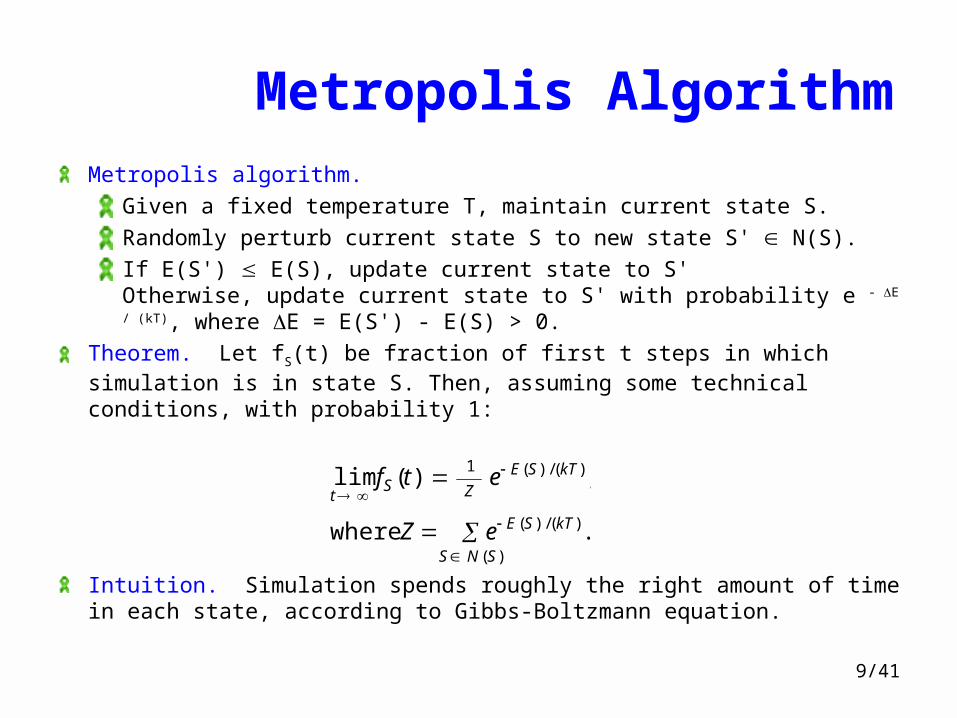
Metropolis algorithm.

Given a fixed temperature T, maintain current state S.

Randomly perturb current state S to new state S' N(S).

If E(S') E(S), update current state to S'Otherwise, update current state to S' with probability e - E / (kT), where E = E(S') - E(S) > 0.

Theorem. Let fS(t) be fraction of first t steps in which simulation is in state S. Then, assuming some technical conditions, with probability 1:

Intuition. Simulation spends roughly the right amount of time in each state, according to Gibbs-Boltzmann equation.

limt

fS (t) 1

Ze E(S ) /(kT ) ,

where Z e E(S ) /(kT )

S N (S ) .

10/41

Simulated Annealing

Simulated annealing. (Biased towards “downhill”, but also accept “uphill” move )

T large probability of accepting an uphill move is large.T small uphill moves are almost never accepted.Idea: turn knob to control T.Cooling schedule: T = T(i) at iteration i.

Physical analog.Take solid and raise it to high temperature, we do not expect it to maintain a nice crystal structure.Take a molten solid and freeze it very abruptly, we do not expect to get a perfect crystal either.Annealing: cool material gradually from high temperature, allowing it to reach equilibrium at succession of intermediate lower temperatures.

11/41

Hopfield Neural Networks

12/41


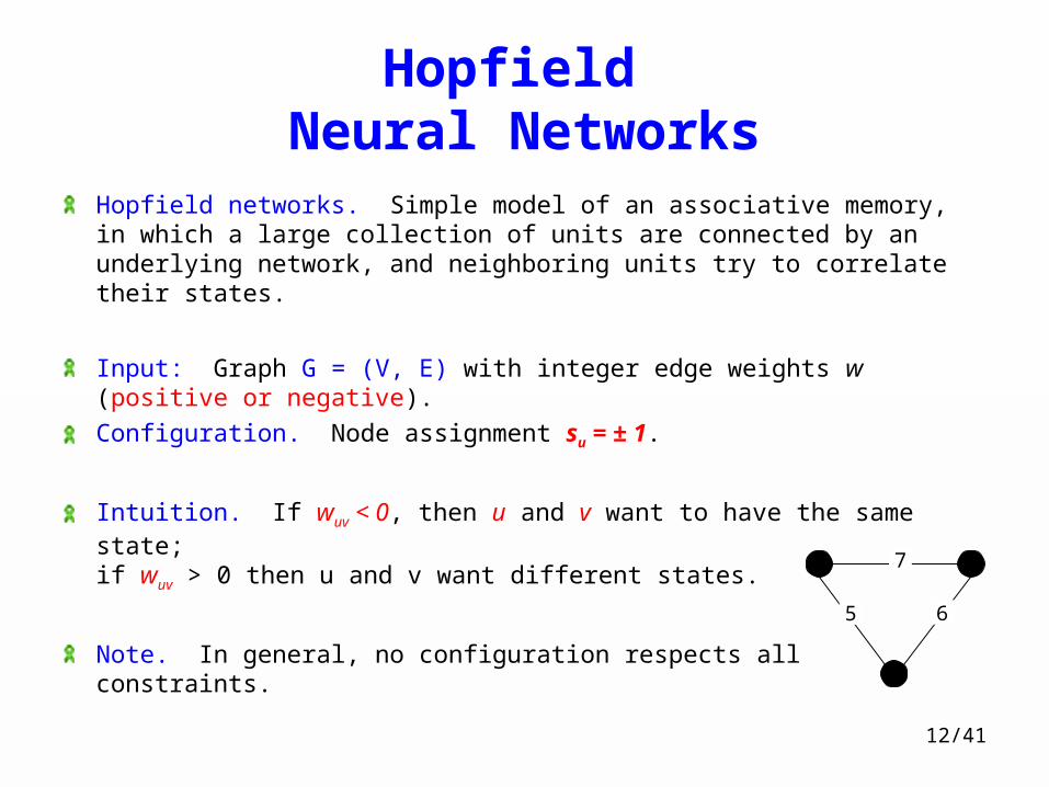
Hopfield networks. Simple model of an associative memory, in which a large collection of units are connected by an underlying network, and neighboring units try to correlate their states.

Input: Graph G = (V, E) with integer edge weights w (positive or negative).

Configuration. Node assignment su = ± 1.

Intuition. If wuv < 0, then u and v want to have the same state;if wuv > 0 then u and v want different states.

Note. In general, no configuration respects all constraints.

5

7

6

13/41


Def. With respect to a configuration S, edge e = (u, v) is good if we su sv < 0.

That is, if we < 0 then su = sv; if we > 0, su sv.

Def. With respect to a configuration S, a node u is satisfied if the weight of incident good edges weight of incident bad edges.

14/41


Def. A configuration is stable if all nodes are satisfied.

Goal. Find a stable configuration, if such a configuration exists.

-5

-10

4

-1

-1

bad edge

satisfied node: 5 - 4 - 1 - 1 < 0

15/41


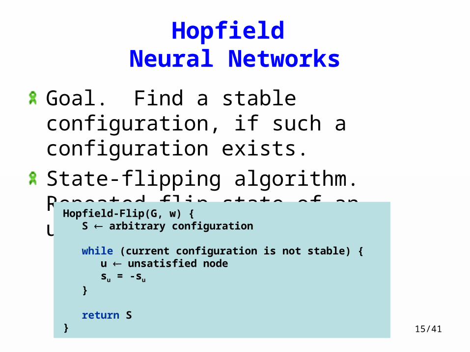
Goal. Find a stable configuration, if such a configuration exists.

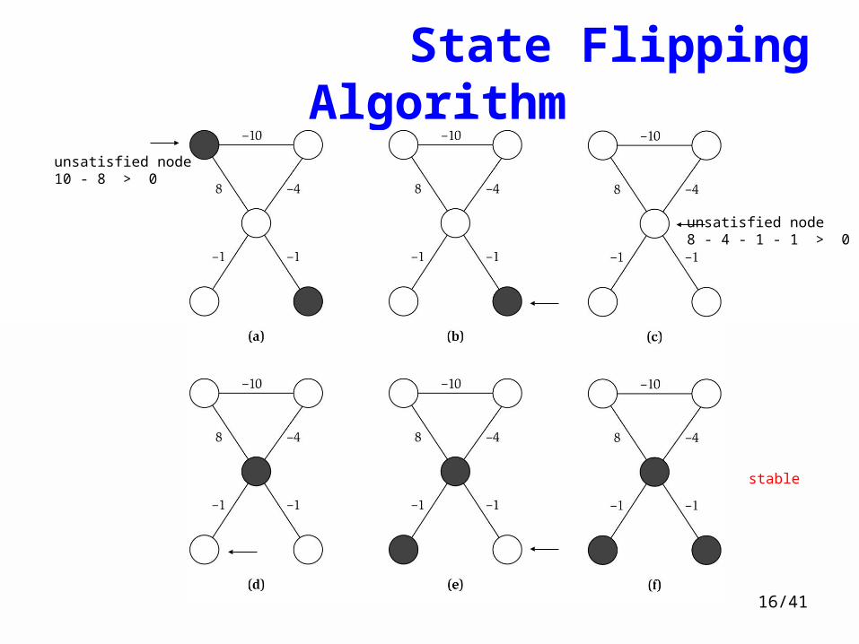
State-flipping algorithm. Repeated flip state of an unsatisfied node.

Hopfield-Flip(G, w) { S arbitrary configuration

while (current configuration is not stable) { u unsatisfied node su = -su

}

return S}

16/41

State Flipping Algorithm

unsatisfied node10 - 8 > 0

unsatisfied node8 - 4 - 1 - 1 > 0

stable

17/41


Claim. State-flipping algorithm terminates with a stable configuration after at most W = e|we| iterations.

Pf attempt. Consider measure of progress (S) = # satisfied nodes.

18


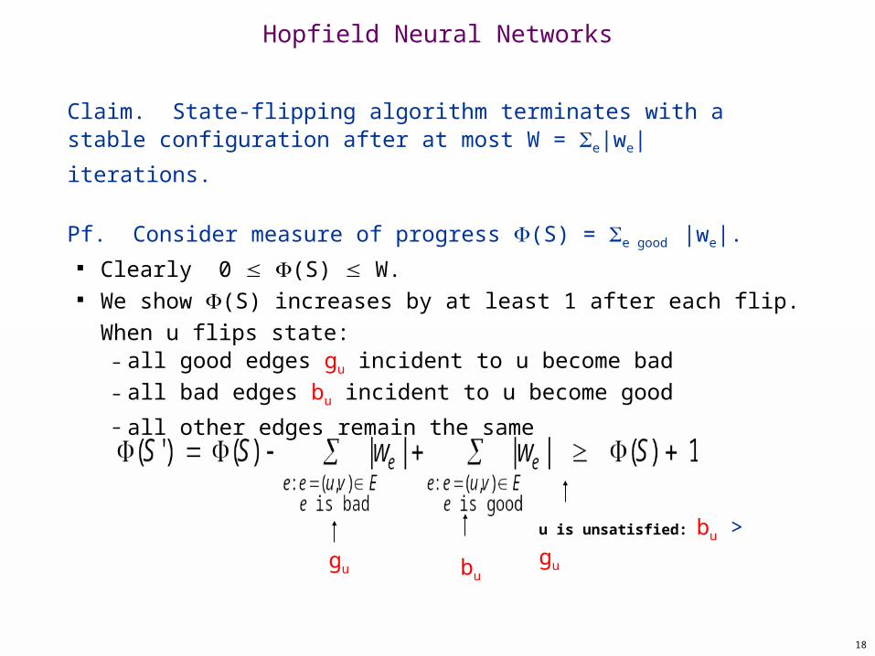
Claim. State-flipping algorithm terminates with a stable configuration after at most W = e|we| iterations.

Pf. Consider measure of progress (S) = e good |we|. Clearly 0 (S) W. We show (S) increases by at least 1 after each flip.

When u flips state:– all good edges gu incident to u become bad– all bad edges bu incident to u become good

– all other edges remain the same

u is unsatisfied: bu > gu

gu bu

19/41

Complexity of Hopfield Neural Network

Hopfield network search problem. Given a weighted graph, find a stable configuration if one exists.

Hopfield network decision problem. Given a weighted graph, does there exist a stable configuration?

Remark. The decision problem is trivially solvable (always yes), but there is no known poly-time algorithm for the search problem.

polynomial in n and log W

20/41

Maximum Cut

21/41

Maximum Cut

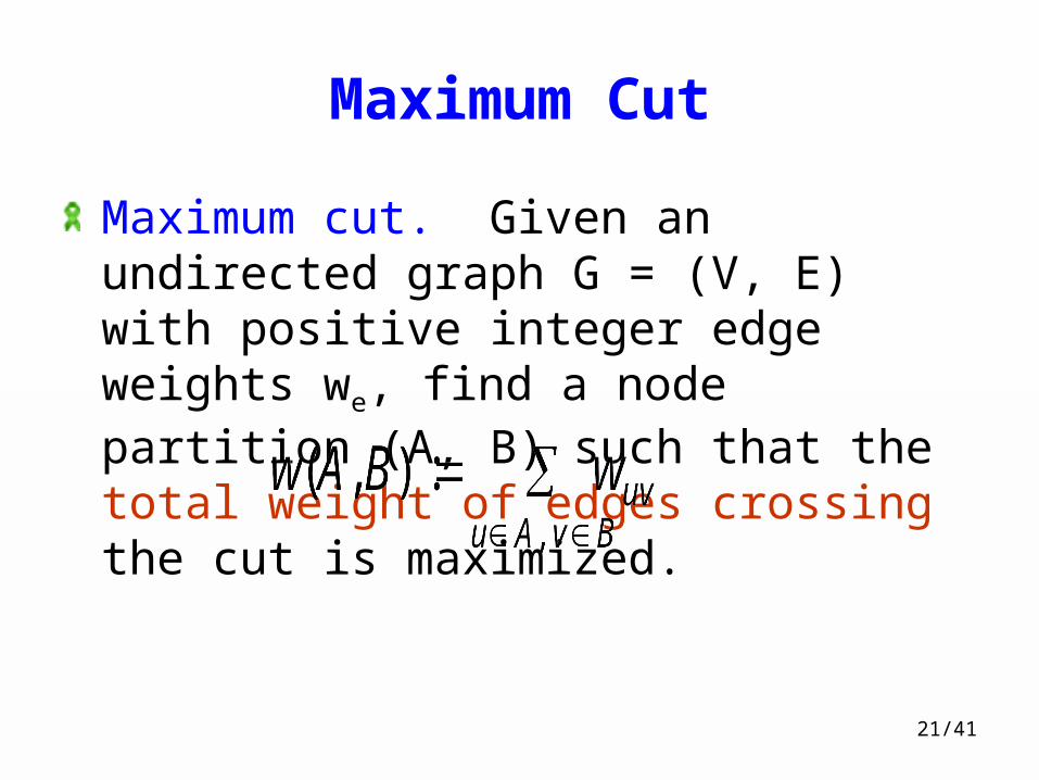
Maximum cut. Given an undirected graph G = (V, E) with positive integer edge weights we, find a node partition (A, B) such that the total weight of edges crossing the cut is maximized.

22/41

Applications

Toy application.

n activities, m people.

Each person wants to participate in two of the activities.

Schedule each activity in the morning or afternoon to maximize number of people that can enjoy both activities.

Real applications. Circuit layout, statistical physics.

23/41

Maximum Cut

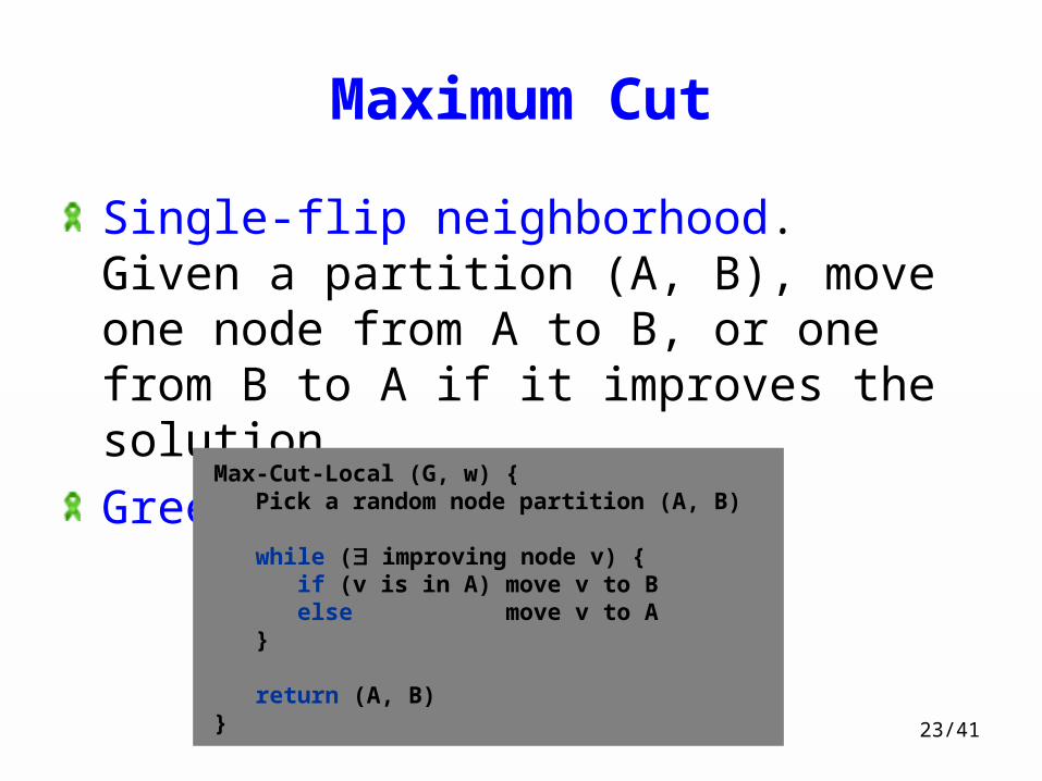
Single-flip neighborhood. Given a partition (A, B), move one node from A to B, or one from B to A if it improves the solution.

Greedy algorithm.

Max-Cut-Local (G, w) { Pick a random node partition (A, B)

while ( improving node v) { if (v is in A) move v to B else move v to A }

return (A, B)}

24/41

Maximum Cut: Local Search Analysis

Theorem. Let (A, B) be a locally optimal partition and let (A*, B*) be optimal partition. Then w(A, B) ½ e we ½ w(A*, B*).

Pf. Local optimality implies that for all u A :

Adding up all these inequalities yields:

25/41

Proof. Con.

Similarly

Now,{ , } , { , }

( , )1 1( , ) ( , )

2 2

2 ( , )e uv uv uve E u v A u A v B u v B

w A Bw A B w A B

w w w w w A B

26/41

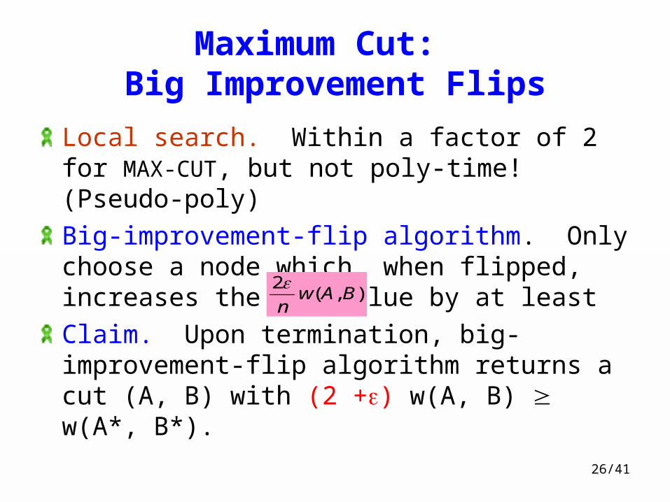
Maximum Cut: Big Improvement Flips

Local search. Within a factor of 2 for MAX-CUT, but not poly-time! (Pseudo-poly)

Big-improvement-flip algorithm. Only choose a node which, when flipped, increases the cut value by at least

Claim. Upon termination, big-improvement-flip algorithm returns a cut (A, B) with (2 +) w(A, B) w(A*, B*).

2( , )w A B

n

27/41

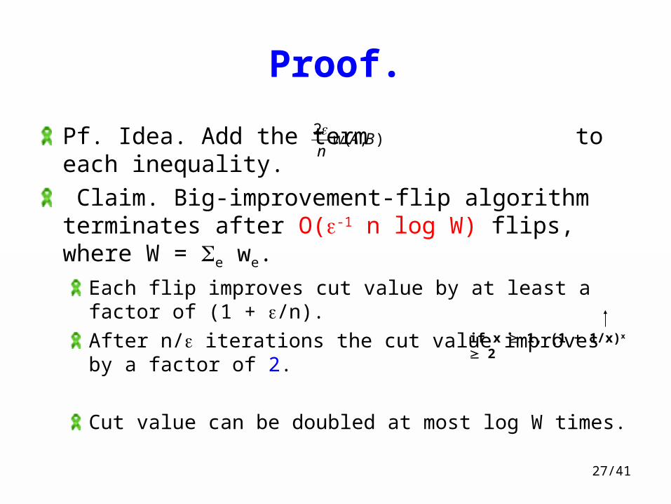
Proof.

Pf. Idea. Add the term to each inequality.

Claim. Big-improvement-flip algorithm terminates after O(-1 n log W) flips, where W = e we.

Each flip improves cut value by at least a factor of (1 + /n).

After n/ iterations the cut value improves by a factor of 2.

Cut value can be doubled at most log W times.

2( , )w A B

n

if x 1, (1 + 1/x)x 2

28/41

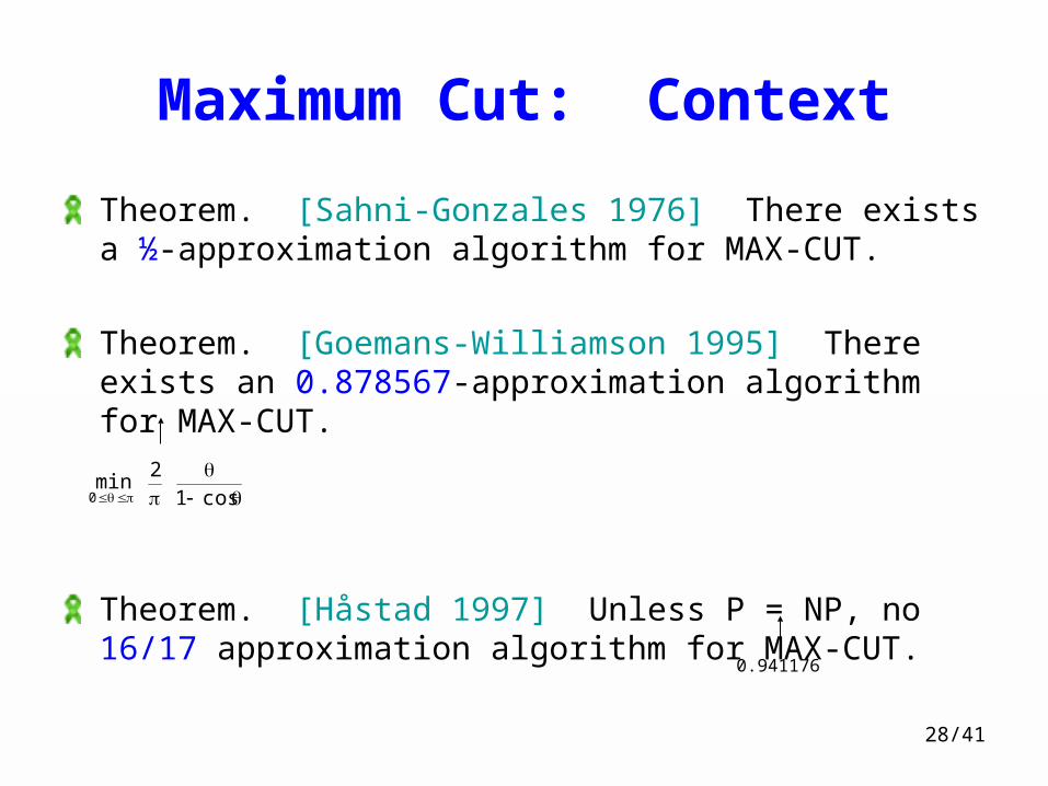
Maximum Cut: Context

Theorem. [Sahni-Gonzales 1976] There exists a ½-approximation algorithm for MAX-CUT.

Theorem. [Goemans-Williamson 1995] There exists an 0.878567-approximation algorithm for MAX-CUT.

Theorem. [Håstad 1997] Unless P = NP, no 16/17 approximation algorithm for MAX-CUT.

0.941176

min0

2

1 cos

29/41

Neighbor Relations

1-flip neighborhood. (A, B) and (A', B') differ in exactly one node.

k-flip neighborhood. (A, B) and (A', B') differ in at most k nodes.

(nk) neighbors.

30/41

Neighbor Relations

KL-neighborhood. [Kernighan-Lin 1970]To form neighborhood of (A, B):

Iteration 1: flip node from (A, B) that results in best cut value (A1, B1), and mark that node.

Iteration i: flip node from (Ai-1, Bi-1) that results in best cut value (Ai, Bi) among all nodes not yet marked.

Neighborhood of (A, B) = (A1, B1), …, (An-1, Bn-1).Neighborhood includes some very long sequences of flips, but without the computational overhead of a k-flip neighborhood.Practice: powerful and useful framework.Theory: explain and understand its success in practice.

31/41

Nash Equilibria

32/41

Multicast Routing

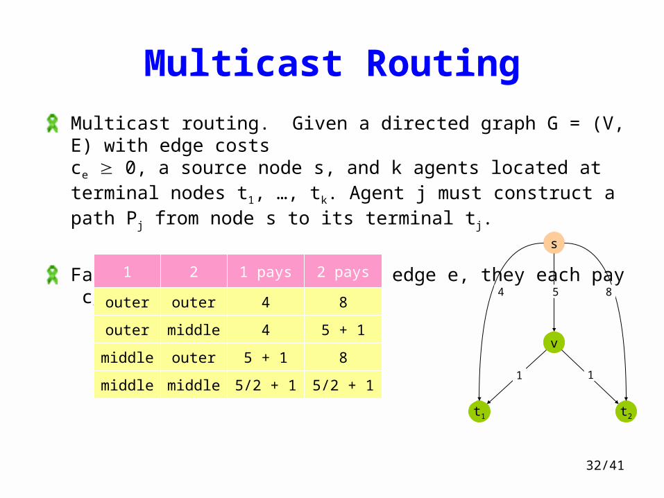
Multicast routing. Given a directed graph G = (V, E) with edge costsce 0, a source node s, and k agents located at terminal nodes t1, …, tk. Agent j must construct a path Pj from node s to its terminal tj.

Fair share. If x agents use edge e, they each pay ce / x.

outer

2

outer

middle

4

1 pays

5 + 1

5/2 + 1

middle 4

1

outer

middle

middle

outer

8

2 pays

8

5/2 + 1

5 + 1

s

t1

v

t2

4 8

1 1

5

33/41

Nash EquilibriumBest response dynamics. Each agent is continually prepared to improve its solution in response to changes made by other agents.

Nash equilibrium. Solution where no agent has an incentive to switch.

Fundamental question. When do Nash equilibria exist?

Ex:

Two agents start with outer paths.

Agent 1 has no incentive to switch paths(since 4 < 5 + 1), but agent 2 does (since 8 > 5 + 1).

Once this happens, agent 1 prefers middlepath (since 4 > 5/2 + 1).

Both agents using middle path is a Nashequilibrium.

s

t1

v

t2

4 5 8

1 1

34/41

Nash Equilibrium and Local Search

Local search algorithm. Each agent is continually prepared to improve its solution in response to changes made by other agents.

Analogies.

Nash equilibrium : local search.

Best response dynamics : local search algorithm.

Unilateral move by single agent : local neighborhood.

Contrast. Best-response dynamics need not terminate since no single objective function is being optimized.

35/41

Socially Optimum

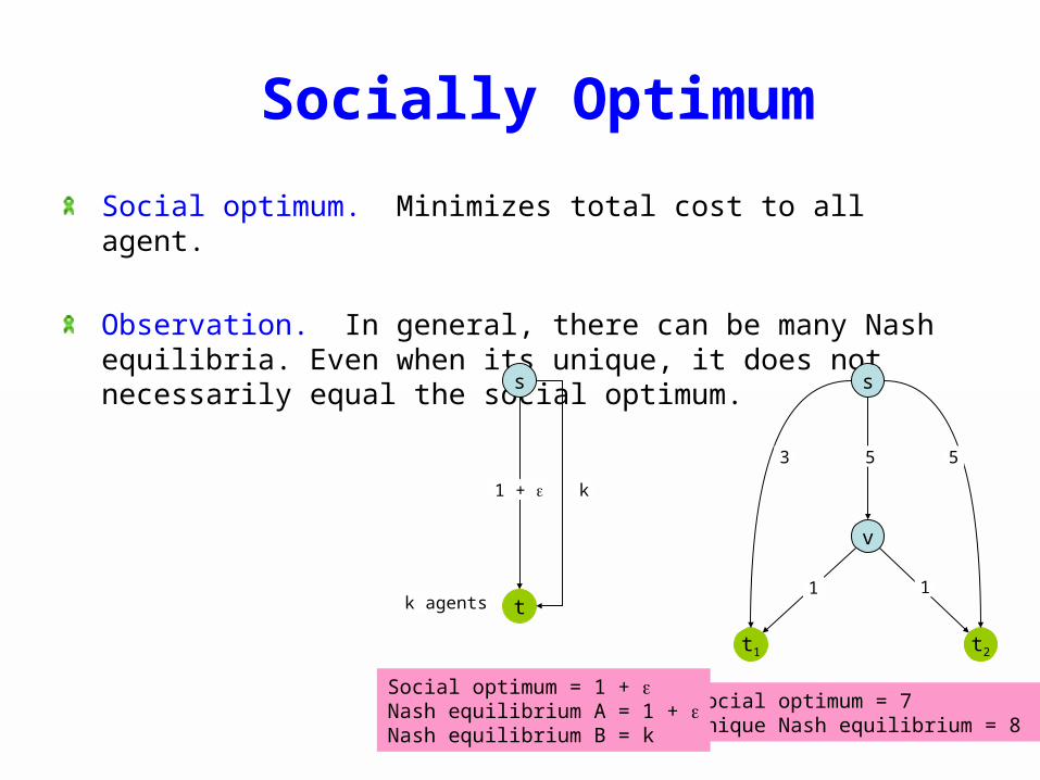
Social optimum. Minimizes total cost to all agent.

Observation. In general, there can be many Nash equilibria. Even when its unique, it does not necessarily equal the social optimum.

s

t1

v

t2

3 5 5

1 1

Social optimum = 7Unique Nash equilibrium = 8

s

t

k1 +

Social optimum = 1 + Nash equilibrium A = 1 + Nash equilibrium B = k

k agents

36/41

Price of StabilityPrice of stability. Ratio of best Nash equilibrium to social optimum.

Fundamental questionFundamental question: What is price of stability?

Ex: Price of stability = (log k).

Social optimum. Everyone takes bottom paths.

Unique Nash equilibrium. Everyone takes top paths.

Price of stability. H(k) / (1 + ). s

t2 t3 tkt1. . .

1 1/2 1/3 1/k

s

0 0 0 0

1 +

1 + 1/2 + … + 1/k

37/41

Finding a Nash Equilibrium

Theorem. The following algorithm terminates with a Nash equilibrium.

Pf. Consider a set of paths P1, …, Pk.

Let xe denote the number of paths that use edge e.

Let (P1, …, Pk) = eE ce· H(xe) be a potential function.

Since there are only finitely many sets of paths, it suffices to show that strictly decreases in each step.

Best-Response-Dynamics(G, c) { Pick a path for each agent

while (not a Nash equilibrium) { Pick an agent i who can improve by switching paths Switch path of agent i }}

H(0) = 0,

H (k) 1

ii1

k

38/41

Finding a Nash Equilibrium

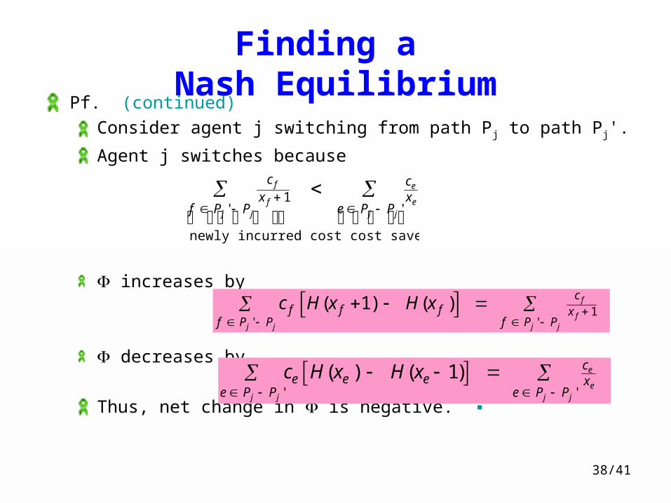
Pf. (continued)

Consider agent j switching from path Pj to path Pj'.

Agent j switches because

increases by

decreases by

Thus, net change in is negative. ▪

c f

x f 1f Pj ' Pj

newly incurred cost

ce

xee Pj Pj '

cost saved

c f H(x f 1) H(x f ) f Pj ' Pj

c f

x f 1 f Pj ' Pj

ce H(xe ) H(xe 1) e Pj Pj '

ce

xe

e Pj Pj '

39/41

Bounding the Price of Stability

Claim. Let C(P1, …, Pk) denote the total cost of selecting paths P1, …, Pk.

For any set of paths P1, …, Pk , we have

Pf. Let xe denote the number of paths containing edge e.

Let E+ denote set of edges that belong to at least one of the paths.

C(P1,, Pk ) cee E ce H(xe )

e E

(P1,, Pk )

ce H(k) H(k)e E C(P1,, Pk )

C(P1,, Pk ) (P1,, Pk ) H(k) C(P1,, Pk )

40/41

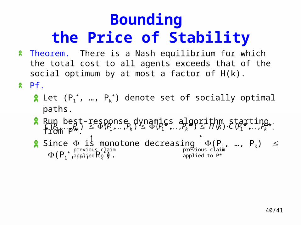
Bounding the Price of Stability

Theorem. There is a Nash equilibrium for which the total cost to all agents exceeds that of the social optimum by at most a factor of H(k).

Pf.

Let (P1*, …, Pk

*) denote set of socially optimal paths.

Run best-response dynamics algorithm starting from P*.

Since is monotone decreasing (P1, …, Pk) (P1*, …, Pk

*).

C(P1,, Pk ) (P1,, Pk ) (P1*,, Pk *) H(k) C(P1*,, Pk *)

previous claimapplied to P

previous claimapplied to P*

41/41

Summary

Existence. Nash equilibria always exist for k-agent multicast routing with fair sharing.

Price of stability. Best Nash equilibrium is never more than a factor of H(k) worse than the social optimum.

Fundamental open problem. Find any Nash equilibria in poly-time.

1/41 local search instructor: ye, deshi [email protected]

Documents