14 protecting private information in online social networks

H. Chen and C.C. Yang (Eds.): Intelligence and Security Informatics, SCI 135, pp. 249 – 273, 2008. springerlink.com © Springer-Verlag Berlin Heidelberg 2008

14

Protecting Private Information in Online Social Networks

Jianming He and Wesley W. Chu

Computer Science Department, University of California, USA {jmhek,wwc}@cs.ucla.edu

Abstract. Because personal information can be inferred from associations with friends, privacy becomes increasingly important as online social network services gain more popularity. Our re-cent study showed that the causal relations among friends in social networks can be modeled by a Bayesian network, and personal attribute values can be inferred with high accuracy from close friends in the social network. Based on these insights, we propose schemes to protect pri-vate information by selectively hiding or falsifying information based on the characteristics of the social network. Both simulation results and analytical studies reveal that selective altera-tions of the social network (relations and/or attribute values) according to our proposed protec-tion rule are much more effective than random alterations.

14.1 Introduction

With the increasing popularity of Web 2.0, more and more online social networks (OSNs) such as Myspace.com, Facebook.com, and Friendster.com have emerged. People in OSNs have their own personalized space where they not only publish their biographies, hobbies, interests, blogs, etc., but also list their friends. Friends or visi-tors can visit these personal spaces and leave comments. OSNs provide platforms where people can place themselves on exhibit and maintain connections with friends, and that is why they are so popular with the younger generation. However, as more people use OSNs, privacy becomes an important issue. When considering the multi-tude of user profiles and friendships flooding the OSNs (e.g., Myspace.com claims to have about 100 million membership accounts), we realize how easily information can be divulged if people mishandle it [8]. One example is a school policy violation iden-tified on Facebook.com. In November 2005, four students at Northern Kentucky Uni-versity were fined when pictures of a drinking party were posted on Facebook.com. The pictures, taken in one of NKU’s dormitories, were visual proof that the students were in violation of the university’s dry campus policy. In this example, people’s pri-vate activities were disclosed by themselves.

There is another type of privacy disclosure that is more difficult to identify and prevent. In this case, private data can be indirectly inferred by adversaries. Intuitively, friends tend to share common traits. For example, high school classmates have similar ages and the same hometown, and members of a dance club like dancing. Therefore, to infer someone’s hometown or interest in dancing, we can check the values of these

250 J. He and W.W. Chu

attributes of his classmates or club mates. In another example, assume Joe does not wish to disclose his salary. However, a third party, such as an insurance company, uses OSNs to obtain a report on Joe’s social network, which includes Joe’s friends and office colleagues and their personal information. After looking carefully into this report, the insurance company realizes that Joe has quite a few friends who are junior web developers of a startup company in San Jose. Thus, the insurance company can deduce that most likely Joe is also a programmer (if this information is not provided by Joe himself). By using the knowledge concerning a junior programmer’s salary range, the insurance company can then figure out Joe’s approximate salary and adver-tise insurance packages accordingly. Therefore, in this example, Joe’s private salary information is indirectly disclosed from Joe’s social relations.

Information privacy is one of the most urgent research issues in building next-generation information systems, and a great deal of research effort has been devoted to protecting people’s privacy. In addition to recent developments in cryptography and security protocols [1, 2] that provide secure data transfer capabilities, there has been work on enforcing industry standards (e.g., P3P [21]) and government policies (e.g., the HIPAA Privacy Rule [19]) to grant individuals control over their own pri-vacy. These existing techniques and policies aim to effectively block direct disclosure of sensitive personal information. However, as we mentioned in the previous exam-ples, private information can also be indirectly deduced by intelligently combining pieces of seemingly innocuous or unrelated information. To the best of our knowl-edge, none of the existing techniques are able to handle such indirect disclosures.

In this chapter we shall discuss how to protect the disclosure of private information that can be inferred from social relations. To preserve the inference properties from the social network characteristics, we encode the causability of a social network into a Bayesian network, and then use simulation and analysis to investigate the effective-ness of inference on private information in a social network. We have conducted an experiment on the Epinions.com that operates in a real environment to verify the per-formance improvements gained by using the Bayesian network for inferring private information. Based on the insights obtained from the experiment, a privacy protection rule has been developed. Privacy protection methods derived from the protection rule are proposed, and their performance is evaluated.

The chapter is organized as follows. After introducing the background in Sect. 14.2, we propose a Bayesian network approach in Sect. 14.3 to infer private informa-tion. Sect. 14.4 discusses simulation experiments for studying the performance of Bayesian inference. Privacy protection rules, as well as protection schemes, are pro-posed and evaluated in Sect. 14.5. In Sect. 14.6 we use analysis to show that based on our protection rules, selective alterations of the social network (social relations and/or attribute values) yield much more effective privacy protection than the random altera-tions. We present some related work on social networks in Sect. 14.7. Finally, future work and conclusions are summarized in Sect. 14.8. Sect. 14.8 is followed by several questions related to the discussion in this chapter.

14.2 Background

A Bayesian network [9, 10, 7, 22] is a graphic representation of the joint probability distribution over a set of variables. It consists of a network structure and a collection

14 Protecting Private Information in Online Social Networks 251

of conditional probability tables (CPT). The network structure is represented as a di-rected acyclic graph (DAG) in which each node corresponds to a random variable and each edge indicates a dependent relationship between connected variables. In addi-tion, each variable (node) in a Bayesian network is associated with a CPT, which enu-merates the conditional probabilities for this variable given all the combinations of its parents’ value. Thus, for a Bayesian network, the DAG captures causal relations among random variables, and CPTs quantify these relations.

Bayesian networks have been extensively applied to fields such as medicine, image processing, and decision support systems. Since Bayesian networks include the con-sideration of network structures, we decided to model social networks with Bayesian networks. Basically, we represent an individual in a social network as a node in a Bayesian network and a relation between individuals in a social network as an edge in a Bayesian network.

14.3 Bayesian Inference Via Social Relations

In this section we propose an approach to map social networks into Bayesian net-works, and then illustrate how we use this for attribute inference. The attribute infer-ence is used to predict the private attribute value of a particular individual, referred to as the target node Z, from his social network which consists of the values of the same attribute of his friends. Note that we do not utilize the values of other attributes of Z and Z’s friends in this study, though considering such information might improve the prediction accuracy. Instead, we only consider a single attribute so that we can focus on the role of social relations in the attribute inference. The single attribute that we study can be any attribute in general, such as gender, ethnicity, and hobbies, and we refer to this attribute as the target attribute. For simplicity, we consider the value of the target attribute as a binary variable, i.e., either true (or t for short) or false (f). For example, if Z likes reading books, then we consider Z’s book attribute value is true.

People are acquainted with each other via different types of relations, and it is not necessary for an individual to have the same attribute values as his friends. Which at-tributes are common between friends depends on the type of relationship. For exam-ple, diabetes could be an inherited trait in family members but this would not apply to officemates. Therefore, to perform attribute inference, we need to filter out the non-related social relations. For instance, we need to remove Z’s officemates from his so-cial network if we want to predict his health condition. If the types of social relations that cause friends to connect with one another are specified in the social networks, then the filtering is straightforward. However, in case such information is not given, one possible solution is to classify social relations into different categories, and then filter out non-related social relations based on the type of the categories. In Sect. 14.4, we show such an example while inferring personal interests from data in Epin-ions.com. For simplicity, in this section we assume that we have already filtered out the non-related social relations, and the social relations we discussed here are the ones that are closely related to the target attribute.

The attribute inference involves two steps. Before we predict the target attribute value of Z, we first construct a Bayesian network from Z’s social network, and then apply a Bayesian inference and obtain the probability that Z has a certain attribute


value. In this section we shall first start with a simple case in which the target attribute values of all the direct friends are known. Then, we extend the study by considering the case where some friends hide their target attribute values.

14.3.1 Single-Hop Inference

Let us first consider the case in which we know the target attribute values of all the di-rect friends of Z. We define Zij as the jth friend of Z at i hops away. If a friend can be reached via more than one route from Z, we use the shortest path as the value of i. Therefore, Z can also be represented as Z00. Let Zi be the set of Zij (0 ≤ j < ni), where ni is the number of Z’s friends at i hops away. For instance, Z1 = {Z10, Z11, ... Z1(n1-1)} is the set of Z’s direct friends who are one hop away. Furthermore, we use the corre-sponding lowercase variable to represent the target attribute value of a particular per-son, e.g., z10 stands for the target attribute value of Z10.

An example of a social network with six friends is shown in Fig. 14.1(a). In this figure, Z10, Z11 and Z12 are direct friends of Z. Z20 and Z30 are the direct friends of Z11 and Z20 respectively. In this scenario, the attribute values of Z10, Z11, Z12 and Z30 are known (represented as shaded nodes).

(a) (b) (c)

Fig. 14.1. Reduction of a social network (a) into a Bayesian network to infer Z from his friends via localization assumption (b), and via naïve Bayesian assumption (c). The shaded nodes rep-resent friends whose attribute values are known.

Bayesian Network Construction

To construct the Bayesian network, we make the following two assumptions. Intuitively, our direct friends have more influence on us than friends who are two

or more hops away. Therefore, to infer the target attribute value of Z, it is sufficient to consider only the direct friends of Z1. Knowing the attribute values of friends at mul-tiple hops away provides no additional information for predicting the target attribute value. Formally, we state this assumption as follows.

Localization Assumption Given the attribute values of the direct friends Z1, friends at more than one hop away (i.e., Zi for i > 1) are conditionally independent of Z.

Based on this assumption, Z20 and Z30 in Fig. 14.1(a) can be pruned, and the infer-ence of Z only involves Z10, Z11 and Z12 (Fig. 14.1(b)). Then the next question is how


to decide a DAG linking the remaining nodes. If the resulting social network does not contain cycles, a Bayesian network is formed. Otherwise, we must employ more so-phisticated techniques to remove cycles, such as the use of auxiliary variables to cap-ture non-causal constraints (exact conversion) and the deletion of edges with the weakest relations (approximation conversion). We adopt the latter approach and make a naive Bayesian assumption. That is, the attribute value of Z influences that of Z1j (0 ≤ j < n1), and there is a direct link pointing from Z to each Z1j. By making this assump-tion, we consider the inference paths from Z to Z1j as the primary correlations, and disregard the correlations among the nodes in Z1. Formally, we have:

Naïve Bayesian Assumption Given the attribute value of the target node Z, the attribute values of direct friends Z1 are conditionally independent of each other.

This naïve Bayesian model has been used in many classification/prediction appli-cations including textual-document classification. Though it simplifies the correlation among variables, this model has been shown to be quite effective [14]. Thus, we also adopted this assumption in our study. For example, a final DAG is formed as shown in Fig. 14.1(c) by removing the connection between Z10 and Z11 in Fig. 14.1(b).

Bayesian Inference

After modeling the specific person Z’s social network into a Bayesian network, we use the Bayes decision rule to predict the attribute value of Z. For a general Bayesian

network with maximum depth i, let Z be the maximum conditional (posterior) prob-ability for the attribute value of Z given the attribute values of other nodes in the net-work, as in Eq. 14.1:

),...,|(maxarg 21 iZ

ZZZZPZ = Z∈{t, f}. (14.1)

Since single-hop inference involves only direct friends Z1 which are independent of each other, the posterior probability can be further reduced using the conditional in-dependence property encoded in the Bayesian network:

,]z) Z|zP(Zz) [P(Z

z) Z|zP(Zz) P(Z

z)] P(Zz) Z|[P(Zz) P(Zz) Z|P(Z

)|(

1-n

0j 1j1j

1-n

0j 1j1j

1

11

1

1

∑ ∏∏

∑

=

=

===

====

=⋅==⋅==

z

z

ZZP

(14.2)

where z and z1j are the attribute values of Z and Z1j respectively (0 ≤ j < n1, z, z1j ∈ {t, f}) and the value of each z1j is known.

To compute Eq. 14.2, we need to further learn the conditional probability table (CPT) for each person in the social network. In our study we apply the parameter


estimation [7] technique on the entire network. For every pair of parent X and child Y, we obtain Eq. 14.3:

( ),

x Xh person wit a connecting links friendship of #y Y and x X with people connecting links friendship of #

|

===

=== xXyYP

(14.3)

where x, y∈{t, f}. P(Y = y | X = x) is the CPT for every pair of friends Z1j and Z in the network. Since P(Z1j | Z) is the same for 0 ≤ j < n1, Z1j becomes equivalent to one an-other, and the posterior probability now depends on N1t, the number of direct friends with attribute value t. We can rewrite the posterior probability P(Z = z | Z1) as P(Z = z | N1t = n1t). Given N1t = n1t, we obtain:

( )

.])|()|()([

)|()|()(

|

111

111

1010

1010

11

∑ −

−

==⋅==⋅===⋅==⋅=

===

z

nnn

nnn

tt

tt

tt

zZfZPzZtZPzZP

zZfZPzZtZPzZP

nNzZP

(14.4)

where z ∈ {t, f}. After obtaining P(Z = t | N1t = n1t) and P(Z = f | N1t = n1t) from Eq. 14.4, we predict Z

has attribute value t if the former value is greater than the latter value, and vice versa.

14.3.2 Multi-hop Inference

In single-hop inference, we assume that we know the attribute values of all the direct friends of Z. However, in reality, not all of those attribute values may be observed since people may hide their sensitive information, and the localization assumption in the previous section is no longer valid. To incorporate more attribute information into our Bayesian network, we propose the following generalized localization assumption.

Generalized Localization Assumption Given the attribute value of the jth friend of Z at i hops away, Zij (0 ≤ j < n1), the at-tribute of Z is conditionally independent of the descendants of Zij.

(a) (b)

Fig. 14.2. Reduction of a social network (a) into a Bayesian network to infer Z from his friends via generalized localization assumption (b). The shaded nodes represent friends whose attribute values are known.


This assumption states that if the attribute value of Z’s direct friend Z1j is unknown, then the attribute value of Z is conditionally dependent on those of the direct friends of Z1j. This process continues until we reach a descendent of Z1j with known attribute value. For example, the network structure in Fig. 14.2(a) is the same as in Fig. 14.1(a), but the attribute value of Z11 is unknown. Based on the generalized local-ization assumption, we extend the network by branching to Z11’s direct child Z20. Since Z20’s attribute value is unknown, we further branch to Z20’s direct friend Z30. The branch terminates here because the attribute value of Z30 is known. Thus, the in-ference network for Z includes all the nodes in the graph. After applying the naive Bayesian assumption, we obtain the DAG shown in Fig. 14.2(b). Similar to single-hop inference, the resulting DAG in multi-hop inference is a tree rooted at the target node Z. One interpretation of this model is that when we predict the attribute value of Z, we always treat Z as an egocentric person who has strong influences on his/her friends. Thus, the attribute value of Z can be reflected by the attributes of friends.

For multi-hop inference, we still apply the Bayes decision rule. Due to additional unknown attribute values such as Z11, the calculation of the posterior probability be-comes more complicated. One common technique for solving this equation is variable

elimination [19]. In this chapter, we use this technique to derive the value of Z in Eq. 14.1.

14.4 Experimental Study of Bayesian Inference

In the previous section we discussed the method for performing the attribute inference in social networks. In this section we study several characteristics of social networks to investigate under what condition and to what extent the value of a target attribute can be inferred by Bayesian inference. Specifically, we study the influence strength between friendship, prior probability of target attributes, and society openness. We use simulations and experiments to evaluate their impact on inference accuracy, which is defined as the percentage of nodes predicted correctly by the inference.

14.4.1 Characteristics of Social Networks

Influence Strength

Analogous to the interaction between inheritance and mutation in biology, we define two types of influence in social relations. More specifically, for the relationship be-tween every pair of parent X and child Y, we define P(Y = t | X = t) (or Pt|t for simpli-fication) as inheritance strength. This value measures the degree to which a child in-herits an attribute value from his/her parent. A higher value of Pt|t implies that both X and Y will possess the attribute value with a higher probability. On the other hand, we define P(Y = t | X = f) (or Pt|f) as mutation strength. Pt|f measures the potential that Y develops an attribute value by mutation rather than inheritance. An individual’s at-tribute value is the result of both types of strength.

There are two other conditional probabilities between X and Y; i.e., P(Y = f | X = t) (or Pf|t) and P(Y = f | X = f) (or Pf|f). These two values can be derived from Pt|t and Pt|f


respectively (Pf|t = 1 – Pt|t and Pf|f = 1 - Pf|f). Therefore, it is sufficient to only consider inheritance and mutation strength.

Prior Probability

Prior probability P(Z = t) (or Pt for short) is the percentage of people in the social network who have the target attribute value as t. When no additional information is provided, we can use prior probability to predict attribute values for the target nodes: if Pt ≥ 0.5, we predict that every target node has value t; otherwise, we predict that it has value f. We call this method naive inference. The average naive inference accu-racy that can be obtained is max(Pt, 1 - Pt). In our study, we use it as a base line for comparison with the Bayesian inference approach.

It is worth pointing out that when Pt|t = Pt, people in a society are in fact independ-ent of each other, thus Pt|t = Pt. Hence, having additional information about a friend provides no contribution to the prediction for the target node.

Society Openness

We define society openness OA as the percentage of people in a social network who release their target attribute value A. The more people who release their values, the higher the society openness, and the more information observed about attribute A. Us-ing society openness, we study the amount of information needed to know about other people in the social network in order to make a correct prediction.

14.4.2 Data Set

For the simulation, we collect 66,766 personal profiles from an online weblog service provider, Livejournal [12], which has 2.6 million active members all over the world. For each member, Livejournal generates a personal profile that specifies the mem-ber’s biography as well as a list of his friends. Among the collected profiles, there are 4,031,348 friend relationships. The degree of the number of friends follows the power law distribu tion (Fig. 14.3). About half of the population has less than ten direct friends.

1

10

100

1000

10000

1 10 100 1000

Num

ber

of M

embe

rs

Number of Direct Friends

Livejournal Link Distribution

Fig. 14.3. Number of direct friends vs. number of members in Livejournal on a log-log scale


In order to evaluate the inference behaviors for a wide range of parameters, we use a hypothetical attribute and synthesize the attribute values. For each member, we as-sign a CPT and determine the actual attribute value based on the parent’s value and the assigned CPT. The attribute assignment starts from the set of nodes whose in-degree is zero and explores the rest of the network following friendship links. We use the same CPT for each member. For all the experiments, we evaluate the inference performance by varying CPTs.

After the attribute assignment, we obtain a social network. To infer each individ-ual, we build a corresponding Bayesian network and then conduct Bayesian inference as described in Sect. 14.3.

14.4.3 Simulation Results

Comparison of Bayesian and Naive Inference

In this set of experiments, we compare the performance of Bayesian inference to na-ïve inference. We shall study whether privacy can be inferred from social relations. We fix the prior probability Pt to 0.3 and vary inheritance strength Pt|t from 0.1 to 0.9.1 We perform inference using both approaches on every member in the network. The inference accuracy is obtained by comparing the predicted values with the

0.65

0.7

0.75

0.8

0.85

0.9

0.95

1

0 0.2 0.4 0.6 0.8 1

Infe

renc

e A

ccur

acy

Inheritance Strength

Naive InferenceBayesian Inference

Fig. 14.4. Inference accuracy of Bayesian vs. naive inference when Pt = 0.3

corresponding actual values. Fig. 14.4 shows the inference accuracy of the two methods as the inheritance strength, Pt|t, increases. It is clear that Bayesian inference outperforms naïve inference. The curve for naïve inference fluctuates around 70%, because with Pt = 0.3, the average accuracy we can achieve is 70%. The performance of Bayesian inference varies with Pt|t. We achieve a very high accuracy, especially at high inheritance strength. The accuracy reaches 95% when Pt|t = 0.9, which is much higher than the 70% accuracy of the naïve inference. Similar trends are observed be-tween these two methods for other prior probabilities as well.

1 In an equilibrium state, the value of Pt|f can be derived from Pt and Pt|t. When Pt is fixed, in-

creasing Pt|t results in a decrease in Pt|f.


Effect of Influence Strength and Prior Probability

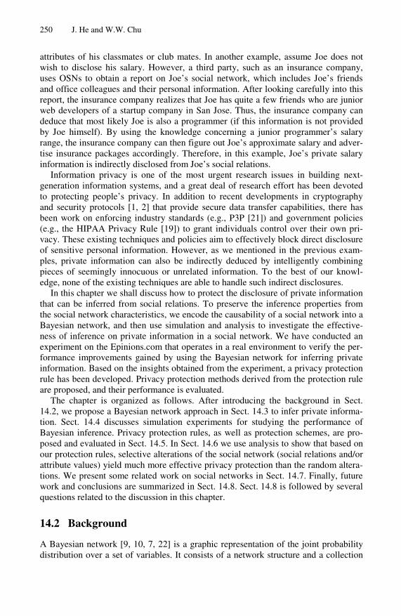
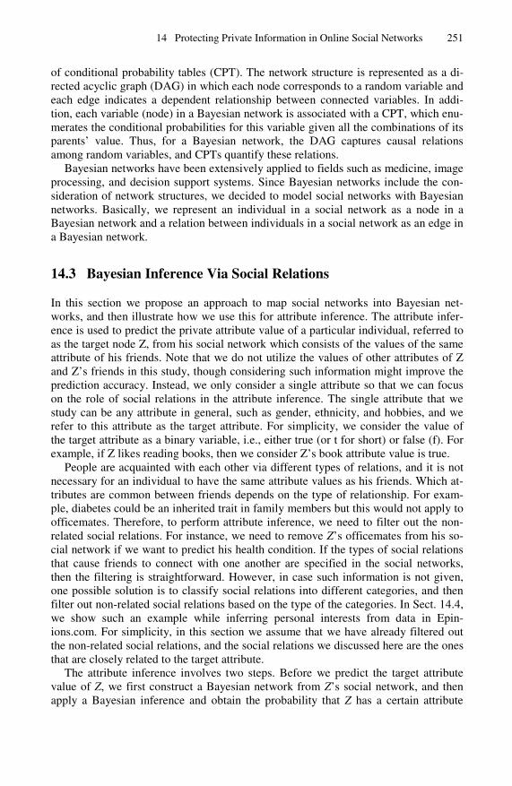
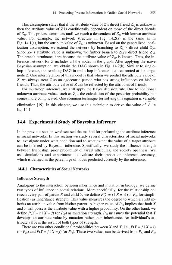
Fig. 14.5 shows the accuracy of Bayesian inference when the prior probability Pt is 0.05, 0.1, 0.3 and 0.5, and the inheritance strength Pt|t varies from 0.1 to 0.9. As Pt varies, the inference accuracy yields different trends with Pt|t. The lowest inference accuracy always occurs when Pt|t is equal to Pt. For example, the lowest inference ac-curacy (approximately 70%) at Pt = 0.3 occurs when Pt|t is 0.3. At this point, people in the network are independent of each another. The inference accuracy increases as the difference between Pt|t and Pt increases.

0

0.2

0.4

0.6

0.8

1

1.2

0 0.2 0.4 0.6 0.8 1

Infe

renc

e A

ccur

acy


Pt=0.05Pt=0.1Pt=0.3Pt=0.5

Fig. 14.5. Inference accuracy of Bayesian inference for different prior probabilities

Society Openness

In the previous experiments, we assumed that society openness is 100%. That is, the attribute values of all the friends of the target node are known. In this set of experi-ments, we study the inference behavior at different levels of society openness. We randomly hide the attribute values of a certain percentage of members, ranging from 10% to 90%, and then perform Bayesian inference on those members.

Fig. 14.6 shows the experimental results for the prior probability Pt = 0.3 and the society openness OA = 10%, 50% and 90%. The inference accuracy decreases as the openness decreases (i.e., the number of members hiding their attribute values in-creases). For instance, at inheritance strength 0.7, when the openness is decreased from 90% to 10%, the accuracy reduces from 84.6% to 81.5%. However, the reduc-tion in inference accuracy is relatively small (on average less than 5%). We also ob-serve similar trends for other prior probabilities. This phenomenon reveals that ran-domly hiding friends’ attribute values only results in a small effect on the inference accuracy. Therefore, we should consider selectively altering social networks to im-prove privacy protection.

Robustness of Bayesian Inference on False Information

To evaluate the robustness of Bayesian inference when people provide false informa-tion, we control the percentage of members (from 0% to100%) who can randomly set


0.65

0.7

0.75

0.8

0.85

0.9

0.95

1

0 0.2 0.4 0.6 0.8 1

Infe

ren

ce A

ccu

racy


OA=10%OA=50%OA=90%

Fig. 14.6. Inference accuracy of Bayesian inference for different society openness when Pt = 0.3

their attribute values (referred to as randomness). Fig. 14.7 shows the impact of ran-domness on the inference accuracy at prior probability Pt = 0.3 and inheritance strength Pt|t = 0.7. At low randomness, we note that the Bayesian inference clearly has a higher accuracy than the naïve inference. For example, when the randomness is 0.1, the inference accuracy of Bayesian and naïve inferences is 79.7% and 72.9% respec-tively. However, the advantage of Bayesian inference decreases as the randomness in-creases. This is especially so when the randomness reaches 1.0. At that point, there is almost no difference in the inference accuracy between Bayesian and naïve infer-ences. This is because their attribute values no longer follow the causal relations be-tween friends when they randomly negate their attribute values. As a result, Bayesian inference behaves similar to naive inference. Thus, from a privacy protection point of view, falsifying personal attribute values can be an effective technique. Based on these characteristics, we will propose several schemes for privacy protection and evaluate their effectiveness in Sect. 14.5.

0

0.2

0.4

0.6

0.8

1

0 0.2 0.4 0.6 0.8 1

Infe

rence

Acc

ura

cy

Randomness

Naive InferenceBayesian Inference

Fig. 14.7. Inference accuracy of Bayesian inference for different randomness when Pt = 0.3 and Pt|t = 0.7


14.4.4 Experiments on Epinions.com

To evaluate the performance of Bayesian inference in a real social network, we con-duct some experiments on Epinions.com [6]. Epinions is a review website for prod-ucts including digital cameras, video games, hotels, restaurants, etc. Epinions divides these products into 23 categories and hundreds of subcategories. We consider that people have interests in a particular category if they write reviews on products in this category. In addition, registered members can also specify members in Epinions that they trust. Thus, a social network is formed where people are connected by trust rela-tions. In this trust network, if person A trusts person B, it is very likely that A also likes the products that B is interested in. In this experiment, we use Bayesian infer-ence to predict people’s interests in some categories from the friends that they trust, and then compared the prediction with the actual categories of their reviews published on Epinions. The higher the percentage of the matches, the better the prediction.

We collect 66,390 personal profiles from Epinions. Each profile represents an in-dividual with his product reviews and the people he trusts. We remove people who have no review and have no friend at all, which reduces the collection to 44,992 per-sonal profiles. On average, each person writes 17 reviews, and has reviews in four categories. Among all categories, the most popular ones are movies, electronics and books. In terms of trust relations, each individual trusts 17 persons on average, and the distribution of the trust relations per user falls into a power law distribution again (as shown in Fig. 14.8).

Before we perform Bayesian inference on Epinions, we need to further prune the social network by filtering out social relations that are not related to the target attrib-ute. Although people in Epinions are connected by trust relations, the persons that an individual trusts may be different from category to category. Since this information is not given in Epinions, we apply a heuristic assumption that friends with similar types of common interests have similar types of relations. We perform a K-means clustering [15] over 23 categories in Epinions. Each cluster represents a group of similar inter-ests. Several examples of clusters are shown in Table 14.1. For example, electronic and computer hardware are clustered together, online store & services is clustered with music and books, etc. Once we have the clusters, we filter out the social relations

1

10

100

1000

10000

1 10 100 1000

Num

ber

of M

embe

rs

Number of Direct Friends

Epinion Link Distribution

Fig. 14.8. Number of direct friends vs. number of members in Epinions on a log-log scale


Table 14.1. Examples of the clustered interests in Epinions

Cluster Health, Personal Finance, Education Online Store & Services, Music, Books Restaurants & Gourmet, Movies Electronics, Computer Hardware

Table 14.2. Inference accuracy comparison between Bayesian and naïve inferences

Accuracy Target Attribute Pt Pt|t Naïve Inference Bayesian Inference

Health 0.461 0.734 53.9% 63.8% Online Store & Services 0.522 0.735 52.2% 60.6% Restaurants & Gourmet 0.432 0.667 56.8% 64.2% Electronics 0.766 0.833 76.6% 76.5%

if connected people have no common interests with others in the cluster. In other words, when predicting the target attribute values of health, we only consider the so-cial relations where connected persons have a common interest in at least one cate-gory in the health cluster, i.e., personal finance, education or health categories. This filtering process reduces the original social network into a more focused social net-work. Once the social network is pruned, we perform Bayesian inference.

Table 14.2 compares the inference accuracy of Bayesian and naïve inferences. Note that the openness used in this experiment is 100%. As we can see from this ta-ble, Bayesian inference achieves higher predictions than the naïve inference. For the health category, the inference accuracy of naïve inference is 53.9%, and the corre-sponding accuracy of Bayesian inference is 63.8%. The results of other attributes show a similar trend, except for the electronics categories. This is because electronics is a very popular interest with prior probability Pt 0.766. Thus, most people will have this interest themselves, and the influence from friends is not comparatively strong enough.

14.5 Privacy Protection

We have shown that private attribute values can be inferred from social relations. One way to prevent such inference is to alter an individual’s social network, which means changing his social relations or the attribute values of his friends. For social relations, we can either hide existing relations or add fraudulent ones. For friends’ attributes, we can either hide or falsify their values. Our study on society openness suggests that random changes on a social network have only a small effect on the result of Bayesian inference. Therefore, an effective protection method requires choosing appropriate candidates for alteration.

In this section we shall study privacy protection schemes. We first present a theorem that captures the causal effect between friends’ attribute values in a chain to-pology. We then apply this theorem to develop our protection schemes. We conduct


experiments on the Livejournal network structure and evaluate the performance of the proposed protection schemes.

14.5.1 Causal Effect between Friends’ Attribute Values

As mentioned earlier, children’s attribute values are the result of the interaction be-tween the inheritance strength Pt|t and the mutation strength Pt|f of their parents. For example, in a family where the inheritance strength is stronger than the mutation strength, children tend to inherit the same attribute value from their parents; thus, the evidence of a child having the attribute value t increases our belief that his/her parent has the same attribute value t. On the contrary, when the inheritance strength is weaker than the mutation strength, parents and children are more likely to have oppo-site attribute values, and the evidence of a child having an attribute value t reduces our belief that his/her parent has the same attribute value t. Inspired by this observa-tion, we derive a theorem to quantify the causal effects between friends’ attribute values.

Theorem: Given a social network with a chain topology, let Z be the target node, Zn0 be Z’s descendant at n hops away. Assuming the attribute value of Zn0 is the only evi-dence observed in this chain, and the prior probability Pt satisfies 0 < Pt < 1, we have P(Z = t | Zn0 = t) > P(Z = t) iff (Pt|t - Pt|f)

n > 0, and P(Z = t | Zn0 = f) > P(Z = t) iff (Pt|t - Pt|f)

n < 0, where Pt|t and Pt|f are the inheritance strength and mutation strength of the network respectively.

Proof: see Appendix.

This theorem states that when Pt|t > Pt|f, the posterior probability P(Z = t | Zn0 = t) is greater than the prior probability P(Z = t). Thus, the evidence of Zn0 = t increases our prediction for Z = t. On the other hand, when Pt|t < Pt|f, whether P(Z = t | Zn0 = t) is greater than P(Z = t) or not also depends on the value of n, i.e., the depth of Zn0. When n is even, the evidence that Zn0 = t will increase our prediction for Z = t. How-ever, when n is odd, the evidence that Zn0 = t will decrease our prediction for Z = t.

14.5.2 A Privacy Protection Rule

Based on the above theorem, we propose a privacy protection rule as follows. Assume the protection goal is to reduce others’ belief that the target node has the attribute value t. We alter the nodes in the social network with attribute value t when Pt|t > Pt|f. The alteration could be: 1) hide or falsify the attribute values of friends who satisfy the above conditions, or 2) hide relationships to friends who satisfy the above condi-tions, or add fraudulent relationships to friends who do not. On the other hand, when Pt|t < Pt|f, we alter nodes with attribute value t when that node is even hops away from the target node; otherwise, we alter nodes with attribute value f. To mislead people into believing the target node possesses an attribute value t, we can apply these tech-niques in the opposite way.

Based on the protection rule, we propose the following four protection schemes:

• Selectively hiding attribute value (SHA). SHA hides the attribute values of appro-priate friends.


• Selectively falsifying attribute value (SFA). SFA falsifies the attribute values of appropriate friends.

• Selectively hiding relationships (SHR). SHR hides the relationship between the target node and selected direct friends. When all the friend relationships of this in-dividual are hidden, the individual becomes a singleton, and the prediction will be made based on the prior probability.

• Selectively adding relationships (SAR). Contrary to hiding relationships in SHR, based on the protection rule, SAR selectively adds fraudulent relationships with people whose attribute values could cause inccorrect inference to the target node

14.5.3 Performance of Privacy Protection

In this section we conduct a set of controlled experiments to evaluate different schemes for privacy protection. To provide privacy protection on an individual’s at-tribute value (target node), we incrementally alter this individual’s social network un-til the attribute value from inference predication changes its value and becomes con-trary to its original value. The protection is considered a failure if it fails to change the attribute value prediction and no further alteration can be made.

We use a randomly hiding attribute value (RHA) as a baseline to evaluate the per-formance of the proposed protection schemes. RHA randomly selects a friend in the individual’s social network and hides his/her attribute value without following the protection rule. We repeatedly perform such operations with the individual’s direct friends. If protection fails after we hide all the direct friends’ attribute values, we pro-ceed to hide attribute values of indirect friends (e.g., at two hops away from this indi-vidual) and so on.

We have performed simulation experiments on 3000 individuals (nodes) in the Livejournal data set. For each node, we apply the above protection schemes and com-pare their performance. The two metrics used are: the percentage of individuals whose attribute values are successfully protected and the average number of alterations needed to reach such protection.

Fig. 14.9 displays the percentage of successful protection for different inheritance strengths Pt|t at Pt = 0.3. We note that the effectiveness of the selected schemes fol-lows the order: SAR > SFA > SHR > SHA > RHA. We shall now discuss the behav-ior of theses schemes to explain and support our experimental findings. For RHA, SHA, SHR and SFA, the maximum number of alterations is the number of descen-dants (e.g., for RHA and SHA) and the number of direct friends (e.g., for SFA and SHR) of the target node. Since SAR can add new friend relationships and support the highest number of alterations to the social network, SAR provides more privacy pro-tectionto the target node. The performance of SFA and SHR follows SAR. We can view SFA as a combination of SHR and SAR, i.e., hiding a friend relationship fol-lowed by adding a fraudulent relationship. Therefore, the performance of SFA is bet-ter than that of SHR. SHA does not perform as well as SFA and SHR because friends at multiple hops away still leave clues for privacy inference. Finally, RHA does not follow the protection rule to take advantage of the properties of the social network, so it yields the worst performance.

Fig. 14.10 presents the performance based on the average number of alterations re-quired to successfully protect the attribute value of a target node. We noted that RHA


0

0.1

0.2

0.3

0.4

0.5

0.6

0 0.2 0.4 0.6 0.8 1

Per

cent

age

of S

ucce

ssfu

l Pro

tect

ion


RHASHASFASHRSAR

Fig. 14.9. Performance comparison of selected schemes based on the percentage of successful protection for Pt = 0.3

0

5

10

15

20

0 0.2 0.4 0.6 0.8 1

Num

ber

of A

ltera

tions

Nee

ded

for

Pro

tect

ion


RHASHASFASHRSAR

Fig. 14.10. Number of alterations required to successfully protect the attribute value of a target node at Pt = 0.3

has the worst and SFA has the best performance among the proposed schemes. The average number of alterations of SHR and SAR are comparable for most cases. Note that the average number of required changes for SAR is higher than that of SHR at Pt|t = 0.2. This is because at the low inheritance strength region, SAR can protect many cases that other schemes cannot protect by adding a large number of fraudulent friend relationships. Finally, SHA performs better than RHA but not as good as the other schemes.

Figs. 14.9 and 14.10 reveal the effectiveness of using the protection rule for deriv-ing privacy protection schemes. Furthermore, SFA can provide successful protection for most cases, yet does not require an excessive number of alterations to the original social network.

14.6 Analysis of RHR and SHR

In the previous section we demonstrated that selective social network alterations based on the protection rule are more effective than the method that does not follow the protection rule. We shall now use analysis to compare the difference between


randomly hiding friend relationships (RHR) and selectively hiding friend relation-ships (SHR). Specifically, we use the frequency of posterior probability variation after hiding friend relationships as a metric. A hiding scheme that has a high frequency of posterior probability variation is considered more effective in privacy protection than that of the low frequency ones.

14.6.1 Randomly Hiding Friend Relationships (RHR)

Hiding friend relationships means removing direct friends of the target node. The so-cial network can be represented as a two-level tree with the target node Z as the root and n1 direct friends Z10, ..., Z1(n1-1) as leaves. We want to derive the probability distri-bution of the posterior probability variation due to randomly hiding friend relation-ships, i.e., the difference between the posterior probability after hiding their attribute values and the corresponding probability of this occurrence.

Let random variables N1t and N’1t be the number of friends having attribute value t before and after hiding h friend relationships, where 0 ≤ h ≤ n1 and max(0, N1t - h) ≤ N’1t ≤ min(N1t, n1 - h). If N1t = n1t and N’1t = n’1t, we can compute the posterior prob-abilities P(Z = t | N1t = n1t) and P(Z = t | N’1t = n’1t) from Eq. 14.4 respectively. Therefore, the posterior probability variation caused by hiding h friend relationships is (Eq. 14.5):

.)''|()|(

)'',|(

1111

1111

tttt

tttt

nNtZPnNtZP

nNnNtZP

==−======Δ

(14.5)

Now we want to derive the probability that each possible value of Δ P(Z = t | N1t = n1t, N’1t = n’1t) occurs. In other words, we want to compute the probability of the joint event N1t = n1t and N’1t = n’1t (before and after hiding friend relationships), which is equal to (Eq. 14.6):

).|''()()'',( 1111111111 tttttttttt nNnNPnNPnNnNP ==⋅==== (14.6)

Initially, if we know Z’s attribute value is Z (z ∈{t, f}), the probability that N1t = n1t follows the Binomial distribution (Eq. 14.7):

.)|(

,)|(

111

111

||1

111

||1

111

tt

tt

nnff

nft

ttt

nntf

ntt

ttt

PPn

nfZnNP

PPn

ntZnNP

−

−

⋅⋅⎟⎟⎠

⎞⎜⎜⎝

⎛===

⋅⋅⎟⎟⎠

⎞⎜⎜⎝

⎛===

(14.7)

By un-conditioning on Z, we obtain (Eq. 14.8):

).|()(

)|()()(

11

1111

fZnNPfZP

tZnNPtZPnNP

tt

tttt

==⋅=+==⋅===

(14.8)


We define ht and hf as the numbers of removed nodes (i.e., hidden friend relation-ships) with attribute value t and f, respectively (ht = n1t – n’1t and hf = h - ht). Then we can compute the conditional probability that N’1t = n’1t given N1t = n1t as (Eq. 14.9):

.)|''(1

111

1111

⎟⎟⎠

⎞⎜⎜⎝

⎛

⎟⎟⎠

⎞⎜⎜⎝

⎛ −⎟⎟⎠

⎞⎜⎜⎝

⎛

===

h

n

h

nn

h

n

nNnNPf

t

t

t

tttt (14.9)

In this equation, the numerator represents the number of ways to remove ht nodes with value t and hf nodes with value f, and the denominator represents the number of combinations when choosing any h nodes from a total of n1 nodes.

Substituting Eq. 14.8 and Eq. 14.9 into Eq. 14.6, we obtain P(N1t = n1t, N’1t = n’1t).

14.6.2 Selectively Hiding Friend Relationships (SHR)

We perform a similar analysis for selectively hiding friend relationships in a two-level tree. Unlike random selection which randomly selects nodes with attribute values t or f, this method follows the protection rules and selects all the nodes with the same at-tribute values to hide. Thus, we can compute Δ P(Z = t | N1t = n1t, N’1t = n’1t) as in the previous section. However, the distribution of posterior probability variation needs to be computed differently.

Given h, the number of nodes to remove, n’1t is deterministic. For example, if we remove nodes with attribute t, then n’1t = m - h; otherwise n’1t = m. Consequently, in the former case (Eq. 14.10),

⎩⎨⎧ =

===,0

),()'',( 11

1111tt

tttt

nNPnNnNP (14.10)

whereas in the latter case (Eq. (11)),

⎩⎨⎧ =

===,0

),()'',( 11

1111tt

tttt

nNPnNnNP (14.11)

where P(N1t = n1t) can be obtained from Eq. 14.8.

14.6.3 Randomly vs. Selectively Hiding Friend Relationships

We first compute the average variation in the posterior probability of both RHR and SHR, as shown in Fig. 14.11. We fix n1 to be ten and vary h from one to nine. The x-axis is the number of friends that we hide, and the y-axis is the posterior probability variation based on Eq. 14.5. Clearly, SHR has higher posterior probability variation than RHR, especially for the case of a large number of hidden friends.

We also plot the histogram of the posterior probability variation Δ P(Z = t | N1t = n1t, N’1t = n’1t). We divide the range of posterior probability variation into ten equal width intervals. Then we compute the probability that the posterior probability varia-tion falls in each interval.

if n’1t = m - h

if n’1t = m

otherwise

otherwise


Fig. 14.12 shows the histogram of the posterior probability variation for RHR and SHR, when the prior probability is 0.3 and the influence strength is 0.7. The x axis represents the intervals and the y axis represents the frequency of the posterior prob-ability variation within the interval. The frequency is derived from Eq. 14.6 for RHR and from Eqs. 14.11 and 14.12 for SHR. For SHR, we remove friends with attribute value t. The maximum number of removed friends k cannot exceed N1t. As a result, we do not consider the cases when n1t < k, and we normalize the frequency results for selectively hiding friends based on the overall probability that n1t ≥ k.

0

0.1

0.2

0.3

0.4

0.5

0.6

0 2 4 6 8 10

Pos

terio

r P

roba

bilit

y V

aria

tion

Number of Hidden Nodes

RHRSHR

Fig. 14.11. Average posterior probability variation for selectively and randomly hiding friend relationships

For RHR, we observe that the variation is less than 0.1 for 70% to 90% of the cases in Fig. 14.12(a). Thus, the posterior probability is unlikely to be varied greatly. In contrast, the posterior probability variation in Fig. 14.12(b) is widely distributed, which means there are noticeable changes in the posterior probability after hiding nodes selectively. This trend is more pronounced when increasing the number of re-moved friends. For example, when h = 8, the frequency of the variation lying between 0.9 and 1.0 is about 28.8% as compared to 1.9% in Fig. 14.12(a). These results show the effectiveness of using the protection rule for privacy protection.

0

0.2

0.4

0.6

0.8

1

0 0.1 0.2 0.3 0.4 0.5 0.6 0.7 0.8 0.9 1

Fre

quen

cy

Posterior Probability Variation

h=2h=4h=6h=8

0

0.2

0.4

0.6

0.8

1

0 0.1 0.2 0.3 0.4 0.5 0.6 0.7 0.8 0.9 1

Fre

quen

cy

Posterior Probability Variation

h=2h=4h=6h=8

(a) (b)

Fig. 14.12. Frequency of posterior probability variation for (a) randomly hiding friend relation-ships, and (b) selectively hiding friend relationships


14.7 Related Work

Social network analysis has been widely used in many areas such as sociology, geog-raphy, psychology and information science. It primarily focuses on the study of social structures and social network modeling. For instance, Milgram’s classic paper [16] in 1967 estimates that every person in the world is only six hops away from one another. The recent success of the Google search engine [3] applies social network ideas to the Internet. In [17] Newman reviews the relationship between graph structures and the dynamic behavior of large networks. The Referral Web project mined social networks from a wide variety of publicly available information [11]. In sociology, social net-works are often modeled as an autocorrelation model [5]. In this model, individuals’ opinions or behaviors are influenced not only by those of others, but also by various other constraints in social networks. It uses a weight matrix to represent people’s in-teractions; however, it is still not very clear how to choose the weight matrix. Leend-ers suggested building the weight matrix based on network structure information like node degrees [13]. Our work, on the other hand, models interpersonal relations using conditional probabilities; this depends on both structure information and personal at-tributes. Furthermore, Domingos and Richardson think that an individual’s decision to buy a product is influenced by his friends, and they propose to model social networks as Markov random fields [4]. Because the social networks that they studied are built from a collaborative filtering database, each person is always connected to a fixed number of people who are most similar to him, which in turn forms a structure of stars with a regular degree. In contrast, we collect social networks directly from real online social network service providers. The number of friends of each individual varies. For the reasons of scalability and computational cost, we model social networks with Bayesian networks.

In terms of privacy protection, a great deal of effort has been devoted to develop-ing cryptography and security protocols to provide security data transfer [1, 2]. Addi-tionally, there are also models that have been developed for preserving individual anonymity in data publishing. Sweeney proposes a K-anonymity model which imposes constraints wherein the released information for each person cannot be re-identified from a group smaller than k [16]. In our study we assume that all the per-sonal information released by the owners can be obtained by anyone in the social network. Under this assumption, we propose techniques to prevent malicious users from inferring private information from social networks.

14.8 Conclusion

We have focused this study on the impact of social relations on privacy disclosure and protection. The causal relations among friends in social networks can be effectively modeled by a Bayesian network, and personal attribute values can be inferred via their social relations. The inference accuracy increases as the influence strength in-creases between friends. Experimental results with real data from Epinions.com vali-date our findings that Bayesian inference provides higher inference accuracies than naïve inference.


Based on the interaction between inheritance strength and mutation strength, and the network structure, a protection rule is developed to provide guidance via selective network alterations (social relations and/or attribute values) to provide privacy protec-tion. Experimental results show that alterations based on the protection rule are far more effective than random alterations. Because large variations of alterations can be provided by falsifying attribute values, this yields the most effective privacy protec-tion among all the proposed methods.

For future study, we plan to investigate the use of multiple attributes to improve in-ference and protection. For example, diet and life style can reduce the risk of heart disease. Such multi-attribute semantic relationships can be obtained via domain ex-perts or data mining. We can exploit this information to cluster target interests for inference.

References

1. Abadi, M., Needham, R.: Prudent Engineering Practice for Cryptographic Protocols. Transactions on Software Engineering 22, 6–15 (1995)

2. Bellovin, S.M., Merritt, M.: Encrypted Key Exchange: Password-Based Protocols Secure Against Dictionary Attacks. In: IEEE Symposium on Security and Privacy, Oakland, Cali-fornia, May 1992, pp. 72–84 (1992)

3. Brin, S., Page, L.: The Anatomy of a Large-Scale Hypertextual Web Search Engine. In: Proceedings of the Seventh International World Wide Web Conference (1998)

4. Domingos, P., Richardson, M.: Mining the Network Value of Customers. In: Proceedings of the Seventh International Conference on Knowledge Discovery and Data Mining (2001)

5. Doreian, P.: Models of Network Effects on Social Actors. In: Freeman, L.C., White, D.R., Romney, K. (eds.) Research Methods in Social Analysis, pp. 295–317. George Mason University Press, Fairfax (1989)

6. Epinions (1999), http://www.epinions.com 7. Friedman, N., Getoor, L., Koller, D., Pfeffer, A.: Learning Probabilistic Relational Mod-

els. In: Proceedings of the 16th International Joint Conference on Artificial Intelligence (IJCAI), Stockholm, Sweden (1999)

8. He, J., Chu, W.W., Liu, Z.: Inferring Privacy Information from Social Networks. In: Me-hrotra, S., Zeng, D.D., Chen, H., Thuraisingham, B., Wang, F.-Y. (eds.) ISI 2006. LNCS, vol. 3975, Springer, Heidelberg (2006)

9. Heckerman, D.: A Tutorial on Learning Bayesian Networks. Technical Report. MSR-TR-95-06 (1995)

10. Heckerman, D., Geiger, D., Chickering, D.M.: Learning Bayesian Networks: The Combi-nation of Knowledge and Statistical Data. In: KDD Workshop, pp. 85–96 (1994)

11. Kautz, H., Selman, B., Shah, M.: Referral Web: Combining Social Networks and Collabo-rative Filtering. Communications of the ACM 40(3), 63–65 (1997)

12. Livejournal (1997), http://www.livejournal.com 13. Leenders, R.T.: Modeling Social Influence Through Network Autocorrelation: Construct-

ing the Weight Matrix. Social Networks 24, 21–47 (2002) 14. Lowd, D., Domingos, P.: Naive Bayes Models for Probability Estimation. In: Proceedings

of the Twenty-Second International Conference on Machine Learning (ICML). ACM Press, Bonn (2005)


15. MacQueen, J.B.: Some Methods for Classification and Analysis of Multivariate Observa-tions. In: Proceedings of 5th Berkeley Symposium on Mathematical Statistics and Prob-ability, vol. 1, pp. 281–297. University of California Press, Berkeley (1967)

16. Milgram, S.: The Small World Problem. Psychology Today (1967) 17. Newman, M.E.: The Structure and Function of Complex Networks. SIAM Review 45(2),

167–256 (2003) 18. Sweeney, L.: K-Anonymity: A Model for Protecting Privacy. International Journal on Un-

certainty, Fuzziness, and Knowledge-Based Systems 10(5) (2002) 19. U.D. of Health and O. for Civil Rights Human Services, Standards for Privacy of Indi-

vidually Identifiable Health Information (2003), http://www.hhs.gov/ocr/combinedregtext.pdf

20. Watts, D.J., Strogatz, S.H.: Collective Dynamics of Small-World Networks. Nature (1998) 21. W.W.W.C. (W3C), The Platform for Privacy Preferences 1.1 (2004),

http://www.w3.org/TR/P3P11/ 22. Zhang, N.L., Poole, D.: Exploiting Causal Independence in Bayesian Network Inference.

Journal of Artificial Intelligence Research 5, 301–328 (1996)

Questions for Discussions

1. What are the reasons that the Bayesian network is suitable for modelling social networks for data inference?

2. What are the challenges in using Bayesian networks to model social networks? 3. Why can social networks improve the accuracy of information inference? 4. How does the privacy protection rule protect private attributes in social networks? 5. How can Bayesian inference accuracy be improved using multiple personal

attributes?

Appendix

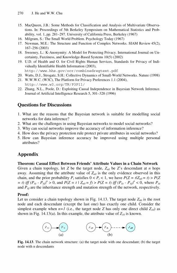
Theorem: Casual Effect Between Friends’ Attribute Values in a Chain Network Given a chain topology, let Z be the target node, Zn0 be Z’s descendant at n hops away. Assuming that the attribute value of Zn0 is the only evidence observed in this chain, and the prior probability Pt satisfies 0 < Pt < 1, we have P(Z = t|Zn0 = t) > P(Z = t) iff (Pt|t - Pt|f)

n > 0, and P(Z = t | Zn0 = f) > P(Z = t) iff (Pt|t - Pt|f)n < 0, where Pt|t

and Pt|f are the inheritance strength and mutation strength of the network, respectively.

Proof: Let us consider a chain topology shown in Fig. 14.13. The target node Z00 is the root node and each descendant (except the last one) has exactly one child. Consider the simplest example when n=1 (i.e., the target node Z has only one direct child Z10) as shown in Fig. 14.13(a). In this example, the attribute value of Z10 is known.

(a) (b)

Fig. 14.13. The chain network structure: (a) the target node with one descendant; (b) the target node with n descendants


Assuming Z10=t, from Eq. 14.1, the posterior probability P(Z00 = t | Z10 = t) is:

.)1(

|()()|()(

)|()(

)|(

||

|

001000001000

001000

1000

fttttt

ttt

PPPP

PP

ZtZPfZPtZtZPtZP

tZtZPtZP

tZtZP

⋅−+⋅⋅

=

=⋅=+==⋅===⋅==

==

(14.12)

Thus,

0

)1()()|(

||

||

|001000

>−⇔

>⋅−+⋅

⋅⇔=>==

fttt

tfttttt

ttt

PP

PPPPP

PPtZPtZtZP

(14.13)

Similarly, when Z10=f, we can prove P(Z00 = t | Z10 = f) > P(Z00 = t) iff Pt|t - Pt|f < 0 for Pt ≠ 1.

Now we extend this example to show how the attribute value of a node at depth n affects the prediction for Z. In Fig. 14.13(b), we show a network of n + 1 nodes. In this figure, only Zn0, Z’s descendent at depth n, has a known value. Fig. 14.14 shows the corresponding conditional probability table for these n+1 nodes.

Fig. 14.14. Conditional probability table for nodes in Fig. 14.13(b)

Let Pttn, Pft

n, Ptfn and Pff

n be the joint distributions of Z and Zn0:

).,(

),,(

),,(

),,(

000

000

000

000

fZfZPP

fZtZPP

tZfZPP

tZtZPP

nnff

nn

tf

nnft

nn

tt

===

===

===

===

(14.14)

for Pt ≠ 1


For example, Ptt1 = P(Z00=t, Z10=t) = P(Z00=t) P(Z10=t|Z00=t) = Pt Pt|t and so on.

We know,

.1)(

,)(

00

00

tnff

nft

tn

tfn

tt

PfZPPP

PtZPPP

−===+

===+

(14.15)

Further, from Fig. 14.14, we have the following relations:

.

)|()|(

,

)|()|(

|1

|1

101

101

|1

|1

101

101

ftnfftt

nft

nnnffnn

nft

nft

ftn

tfttn

tt

nnn

tfnnn

ttn

tt

PPPP

fZtZPPtZtZPPP

PPPP

fZtZPPtZtZPPP

⋅+⋅=

==⋅+==⋅=

⋅+⋅=

==⋅+==⋅=

−−

−−

−−

−−

−−

−− (14.16)

When Zn0=t, the posterior probability is:

.

),(),(),(

)|(000000

000000

nft

ntt

ntt

nn

nn

PP

P

tZfZPtZtZP

tZtZPtZtZP

+=

==+=======

(14.17)

Therefore,

.0)1(

)()|( 00000

>⋅−⋅−⇔

>+

⇔=>==

nftt

nttt

tnft

ntt

ntt

n

PPPP

PPP

PtZPtZtZP

(14.18)

Based on Eq. 14.16,

( )( )[ ] ( )[ ] .11

1

|11

|11

ftnfft

ntfttt

nftt

nttt

nftt

nttt

PPPPPPPPPP

PPPP

⋅⋅−⋅−+⋅⋅−⋅−

=⋅−⋅−−−−−

(14.19)

Substituting Eq. 14.15 into Eq. 14.19, we have

( ) ( )[ ] ( ).11 ||11

ftttnftt

nttt

nftt

nttt PPPPPPPPPP −⋅⋅−⋅−=−− −− (14.20)

Recursively, we have

( ) ( )[ ] ( ) .11 1||

11 −−⋅⋅−⋅−=⋅−⋅− nftttfttttt

nftt

nttt PPPPPPPPPP

(14.21)


Since Ptt1 = Pt Pt|t, and Pft

1 = (1- Pt) Pt|f, we obtain

( )( ) ( )[ ] ( )

( ) ( ) .1

11

1

||

1||||

nfttttt

nftttfttttttt

nftt

nttt

PPPP

PPPPPPPP

PPPP

−⋅−⋅=

−⋅−⋅−⋅⋅−=

⋅−⋅−−

(14.22)

Combining Eq. 14.18 and Eq. 14.22, P(Z00=t | Zn0=t) > Pt is equivalent to (Pt|t - Pt|f)

n > 0 (when 0 < Pt < 1). Similarly, we can show that P(Z00=t | Zn0=f) > Pt is equivalent to (Pt|t - Pt|f)

n < 0.

14 protecting private information in online social networks

Documents