13.472j/1.128j/2.158j/16.940j computational geometry file13.472j/1.128j/2.158j/16.940j computational...
TRANSCRIPT
13.472J/1.128J/2.158J/16.940J
COMPUTATIONAL GEOMETRY
Lectures 10 - 12
N. M. Patrikalakis
Massachusetts Institute of TechnologyCambridge, MA 02139-4307, USA
Copyright c©2003 Massachusetts Institute of Technology
Contents
10.1 Overview of intersection problems . . . . . . . . . . . . . . . . . . . . . . . . . 310.2 Intersection problem classification . . . . . . . . . . . . . . . . . . . . . . . . . 5
10.2.1 Classification by dimension . . . . . . . . . . . . . . . . . . . . . . . . 510.2.2 Classification by type of geometry . . . . . . . . . . . . . . . . . . . . . 510.2.3 Classification by number system . . . . . . . . . . . . . . . . . . . . . . 6
10.3 Point/point “intersection” . . . . . . . . . . . . . . . . . . . . . . . . . . . . . 710.4 Point/curve intersection . . . . . . . . . . . . . . . . . . . . . . . . . . . . . . 8
10.4.1 Point/Implicit curve intersection . . . . . . . . . . . . . . . . . . . . . 810.4.2 Point/Parametric curve intersection . . . . . . . . . . . . . . . . . . . . 1010.4.3 Point/Procedural parametric (offset, evolute, etc.) curve intersection . 12
10.5 Point/surface intersection . . . . . . . . . . . . . . . . . . . . . . . . . . . . . 1310.5.1 Point/Implicit (usually algebraic) surface intersection . . . . . . . . . . 1310.5.2 Point/Rational polynomial surface intersection . . . . . . . . . . . . . . 1310.5.3 Point/Procedural surface intersection . . . . . . . . . . . . . . . . . . . 19
10.6 Curve/curve intersection . . . . . . . . . . . . . . . . . . . . . . . . . . . . . . 2010.6.1 Case D3: RPP/IA curve intersection . . . . . . . . . . . . . . . . . . . 2010.6.2 Case D1: RPP/RPP Curve Intersection . . . . . . . . . . . . . . . . . 2710.6.3 Case D2/D5: RPP/PP and PP/PP Curve Intersections . . . . . . . . . 2810.6.4 Case D6: PP/IA Curve Intersection . . . . . . . . . . . . . . . . . . . . 2810.6.5 Case D8: IA/IA Curve Intersection . . . . . . . . . . . . . . . . . . . . 29
10.7 Curve/surface intersection . . . . . . . . . . . . . . . . . . . . . . . . . . . . . 3010.7.1 Case E3: RPP Curve/IA Surface Intersection . . . . . . . . . . . . . . 3010.7.2 Case E1: RPP Curve/RPP Surface Intersection . . . . . . . . . . . . . 3110.7.3 Case E2/E6: RPP/PP, PP/PP Curve/Surface Intersection . . . . . . . 3110.7.4 Case E7: PP Curve/IA Surface Intersection . . . . . . . . . . . . . . . 31
1

10.7.5 Case E11: IA Curve/IA Surface Intersection . . . . . . . . . . . . . . . 3210.7.6 IA Curve/RPP Surface Intersection . . . . . . . . . . . . . . . . . . . . 33
10.8 Surface/Surface Intersections . . . . . . . . . . . . . . . . . . . . . . . . . . . . 3410.8.1 Case F3: RPP/IA Surface Intersection . . . . . . . . . . . . . . . . . . 3410.8.2 Case F1: RPP/RPP Surface Intersection . . . . . . . . . . . . . . . . . 4210.8.3 Case F8: IA/IA Surface Intersection . . . . . . . . . . . . . . . . . . . 46
10.9 Nonlinear Solvers . . . . . . . . . . . . . . . . . . . . . . . . . . . . . . . . . . 5110.9.1 Motivation . . . . . . . . . . . . . . . . . . . . . . . . . . . . . . . . . . 51
10.10Local Solution Methods . . . . . . . . . . . . . . . . . . . . . . . . . . . . . . 5310.11Classification of Global Solution Methods . . . . . . . . . . . . . . . . . . . . . 5410.12Subdivision Method (Projected Polyhedron Method) . . . . . . . . . . . . . . 5510.13Interval Methods . . . . . . . . . . . . . . . . . . . . . . . . . . . . . . . . . . 60
10.13.1Motivation . . . . . . . . . . . . . . . . . . . . . . . . . . . . . . . . . . 6010.13.2Definitions . . . . . . . . . . . . . . . . . . . . . . . . . . . . . . . . . . 6110.13.3 Interval Arithmetic . . . . . . . . . . . . . . . . . . . . . . . . . . . . . 6210.13.4Algebraic Properties . . . . . . . . . . . . . . . . . . . . . . . . . . . . 6210.13.5Rounded Interval Arithmetic and its Implementation . . . . . . . . . . 62
10.14Interval Projected Polyhedron Algorithm . . . . . . . . . . . . . . . . . . . . . 6510.15Interval Newton method . . . . . . . . . . . . . . . . . . . . . . . . . . . . . . 69
Bibliography 72
Reading in the Textbook
• Chapters 4 and 5, pp. 73 - 160
2

Lectures 10 - 12Intersection Problems, NonlinearSolvers and Robustness Issues
10.1 Overview of intersection problems
Intersections are fundamental in computational geometry, geometric modeling and design,analysis and manufacturing applications. Examples of intersection problems include:
• Shape interrogation (eg. visualization) through contouring (intersection with a series ofparallel planes, coaxial cylinders, and cones etc.)
• Numerical control machining (milling) involving intersection of offset surfaces with aseries of parallel planes, to create machining paths for ball (spherical) cutters.
• Representation of complex geometries in the “Boundary Representation” scheme; forexample, the description of the internal geometry and of structural members of cars,airplanes, ships, etc, involves
– Intersections of free-form parametric surfaces with low order algebraic surfaces(planes, quadrics, torii).
– Intersections of low order algebraic surfaces.
in a process called boundary evaluation, in which the Boundary Representation is cre-ated by “evaluating” the Constructive Solid Geometry model of the object. During thisprocess, intersections of the surfaces of primitives (see Figure 10.1) must be found duringBoolean operations.
Boolean opertations on point sets A, B include (see Figure 10.2)
• Union: A ∪B,
• Intersection: A ∩ B, and
• Difference: A− B.
3

Figure 10.1: Primitive solids.
⇒⇒⇒
Figure 10.2: Example of a Boolean operation: union.
All such operations involve intersections of surfaces to surfaces. In order to solve generalsurface to surface intersection problems, the following auxiliary intersection problems (similarto distance computation problems used in CAM for inspection of manufactured objects) needto be considered
• point/point (P/P)
• point/curve (P/C)
• point/surface (P/S)
• curve/curve (C/C)
• curve/surface (C/S)
All above types of intersection problems are also useful in geometric modeling, robotics,collision avoidance, manufacturing simulation, scientific visualization, etc.
When the geometric elements involved in intersections are nonlinear (curved), intersectionproblems typically reduce to solving complex systems of nonlinear equations, which may beeither polynomial or more general in character. Solution of nonlinear systems is a very com-plex process in general in numerical analysis and there are specialized textbooks on the topic.However, geometric modeling applications pose severe robustness, accuracy, automation, andefficiency requirements on solvers of a nonlinear systems as we will see later. Therefore, geo-metric modeling researchers have developed specialized solvers to address these requirementsexplicitly using geometric formulations.
4
10.2 Intersection problem classification
Intersection problems can be classified according to the dimension of the problems and ac-cording to the type of geometric equations involved in defining the various geometric elements(points, curves and surfaces). The solution of intersection problems can also vary according tothe number system in which the input is expressed and the solution algorithm is implemented.
10.2.1 Classification by dimension
• P/P, P/C, P/S
• C/C, C/S
• S/S
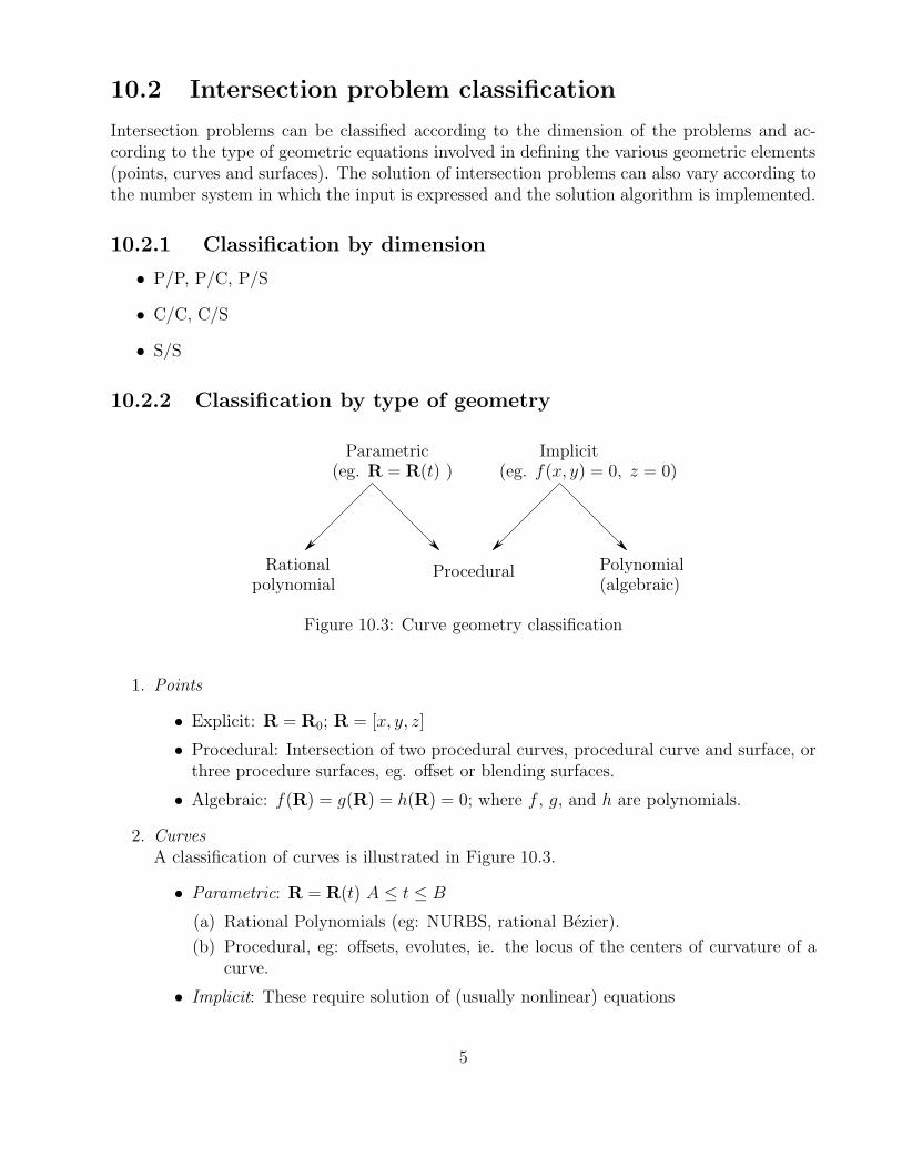
10.2.2 Classification by type of geometry
polynomialProcedural Polynomial
(algebraic)
(eg. f(x, y) = 0, z = 0)Implicit
Rational
Parametric(eg. R = R(t) )
Figure 10.3: Curve geometry classification
1. Points
• Explicit: R = R0; R = [x, y, z]
• Procedural: Intersection of two procedural curves, procedural curve and surface, orthree procedure surfaces, eg. offset or blending surfaces.
• Algebraic: f(R) = g(R) = h(R) = 0; where f , g, and h are polynomials.
2. CurvesA classification of curves is illustrated in Figure 10.3.
• Parametric: R = R(t) A ≤ t ≤ B
(a) Rational Polynomials (eg: NURBS, rational Bezier).
(b) Procedural, eg: offsets, evolutes, ie. the locus of the centers of curvature of acurve.
• Implicit: These require solution of (usually nonlinear) equations
5

(a) Algebraics (polynomial)
f(R) = g(R) = 0 space curves
z = 0, f(x, y) = 0 planar curves
(b) Procedural offsets (eg. non-constant distance offsets involving convolution, seePottmann 1997)
3. Surfaces
• Parametric R = R(u, v) where u, v vary in some finite domain, the parametricspace.
(a) (Rational) Polynomial (eg: NURBS, Bezier, rational Bezier etc.)
(b) Procedural
– offsets
– blends
– generalized cylinders
• Implicit: Algebraicsf(R) = 0
where f is a polynomial.
10.2.3 Classification by number system
In our discussion of intersection problems, we will refer to various classes of numbers:
• integer numbers;
• rational numbers, m/n, n 6= 0, where m,n are integers;
• floating point numbers in a computer (which are a subset of the rational numbers);
• radicals of rational numbers, eg.√
m/n, n 6= 0, where m,n are integers;
• algebraic numbers (roots of polynomials with integer coefficients);
• transcendental (e, π, trigonometric, etc.) numbers.
• real numbers;
• interval numbers, [a, b], where a, b are real numbers;
• rounded interval numbers, [c, d], where c, d are floating point numbers.
Issues relating to floating point and interval numbers affecting the robustness of intersectionalgorithms are addressed in the next section on nonlinear solvers.
6

10.3 Point/point “intersection”
• Check if |R1 − R2| < ε, where ε represents the maximum allowable tolerance.
• Choice of “tolerances” in a geometric modeller is difficult–an open question.
• Lack of transitivity, see Figure 10.4:
R1 = R2
R2 = R3⇒ R1 6= R3
R2
R3
ε
ε.
.
.
R1
Figure 10.4: Intersections of points within a tolerance is intransitive.
• What should ε reflect?
7

10.4 Point/curve intersection
10.4.1 Point/Implicit curve intersection
R0 ∩ {z = 0, f(x, y) = 0}
where f(x, y) is usually a polynomial (and f(x, y) = 0 represents an algebraic curve). In anexact arithmetic context, we can substitute R0 in {z, f(x, y) = 0} and verify if the results arezero. Similarly, we could handle:
R0 ∩ {f(R) = g(R) = 0}where f(R) = g(R) = 0 represents an implicit 3D space curve.
What does verify mean in “floating point” arithmetic?
• Example A:
Let z0 = 0 and x0, y0 satisfy|f(x0, y0)| < ε � 1 (10.1)
where ε is a small constant and |f(x, y)| ≤ 1 in the domain of interest including (x0, y0),then a “distance” check can be performed by:
|f(x0, y0)|| 5 f(x0, y0)|
< δ � 1 (10.2)
provided | 5 f(x0, y0)| 6= 0. Equation 10.1 is called the “algebraic distance” and Equa-tion 10.2 is called the “non-algebraic distance”. The true geometric distance is givenby:
d = min|R − R0|; where R = (x, y), f(R) = 0 (10.3)
The true geometric distance is difficult and expensive to compute (particularly for implicitf(R) = 0 and involves computing the global minimum of |R−R0|. Equation 10.2 resultsfrom the first order approximation of Equation 10.3 as derived by Taylor expansion andis exact when f(R) is represents a plane.
8

.R0 g(R) = 0
f(R) = 0
Figure 10.5: Curves meet at small angle.
• Example B:R0 ∩ {f(R) = g(R) = 0}
When curves f = 0, g = 0 meet at a small angle ( 5f|5f |
· 5g|5g|
∼= 1), then the condition
|f | < ε and δ1 = |f ||5f |
< δ
|g| < ε and δ2 = |g||5g|
< δ
(where |f |, |g|, δ1, δ2 are evaluated with R = R0 and ε, δ � 1) are not enough to guaranteeproximity of R0 to the intersection of f , g, see Figure 10.5.
δ
δ
δ1
2
3
φ
g
f
Figure 10.6: Approximate curves with straight lines.
Using a linear approximation, and letting
φ = cos−1 | 5f| 5 f | ·
5g| 5 g||
be the angle of intersection as in Figure 10.6 near the intersection point, a better criterionfor evaluating if R0 is near the intersection of f and g is
δ3 = φ−1{ |f || 5 f | +
|g|| 5 g|} < δ � 1
9

10.4.2 Point/Parametric curve intersection
1. Rational polynomial curves
R0 ∩ R = R(t) A ≤ t ≤ B
• Brute force elementary method:We solve each of the following three nonlinear polynomial equations separately andwe search for common real roots in A ≤ t ≤ B.
x(t) − x0 = 0 → t′1, · · · , t′ny(t) − y0 = 0 → t′′1, · · · , t′′nz(t) − z0 = 0 → t′′′1 , · · · , t′′′n
In principle, this elementary approach is “easy” for polynomials. However, in prac-tice, this process is complex and inefficient and prone to numerical inaccuracies.
• Preprocessing and subdivision method
– Use bounding box of R(t) to eliminate easily resolvable cases, with some levelof subdivision (splitting) to reduce box size.
– Concept of subdivision in rational arithmetic: To eliminate numerical errorin the subdivision process (which can lead to erroneous decisions), rationalarithmetic may be employed (if the input coefficients of R(t) are rational orfloating point numbers). This can be easily done in object-oriented languagessuch as C++ using operator overloading.
– Continue subdivision until box is small.
– Then, we could use a numerical technique , such as:
F (t) = min{|R0 − R(t)|2} t ∈ D1 ⊂ [A,B]
and use some t from the interval D1 as the initial approximation. Use of thesquare of the distance function is necessary to avoid possible divergence of thederivative of the distance function, if it approaches zero.
– If the minimization process converges to t0 and√
F (t0) < δ, t = t0 is the desiredsolution.
• Implicitization (perhaps with box preprocessing) such as
(x0, y0) ∩ {x = x(t), y = y(t)}
Let us consider an example where x(t), y(t) are quadratic polynomials (the curve isa parabola). We will attempt to eliminate t to get a polynomial f(x, y) = 0 whichthe x, y coordinates of all points on the curve satisfy. We start with the system
x = a0t2 + b0t + c0
y = a′0t2 + b′0t + c′0
⇒ a0t2 + b0t+ c0 − x = 0
a′0t2 + b′0t+ c′0 − y = 0
10

which can be rewritten in matrix form as follows:
⇒
c0 − x b0 a0 00 c0 − x b0 a0
c′0 − y b′0 a′0 00 c′0 − y b′0 a′0
1tt2
t3
=
0000
(10.4)
The maximum degree of t in the above vector is determined by the degree m of thex polynomial and the degree n of the y polynomial, and is given by m + n− 1. Inthis case m+ n− 1 = 3.
A necessary and sufficient condition for the above system to be solvable is
∣∣∣∣∣∣∣∣∣
c0 − x b0 a0 00 c0 − x b0 a0
c′0 − y b′0 a′0 00 c′0 − y b′0 a′0
∣∣∣∣∣∣∣∣∣
= f(x, y) = 0
The equation f(x, y) = 0 is the implicit equation of the curve. Consequently in anexact arithmetic context, we need to check if f(x0, y0) = 0, to verify if (x0, y0) is onthe initial curve.
In general, ifx = x(tn), y = y(tn) ⇒ F (xn, yn) = 0
where n is the total degree.
• Inversion: If f(x, y) = 0 then we could use the first 3 equations 10.4:
b0 a0 0c0 − x0 b0 a0
b′0 a′0 0
tt2
t3
= −
c0 − x0
0c′0 − y0
⇒ t =φ(x0, y0)
ψ(x0, y0)
Where φ and ψ are polynomials in x0 and y0, and x0, y0 satisfy
f(x0, y0) = 0
– The method is efficient and (usually) accurate for n ≤ 3 (but no real guaran-tees on accuracy and robustness exist if the method is implemented in floatingpoint).
– Subdivision methods are preferable for higher n, and as we will see later whencoupled with rounded interval arithmetic are robust, accurate and efficient.
Intersection of points (x0, y0, z0) and 3D polynomial curves R = R(t) via implicit-ization of such curves involves a process of projection on x, y plane and finding t0by inversion and verification of z0 = z(t0).
11
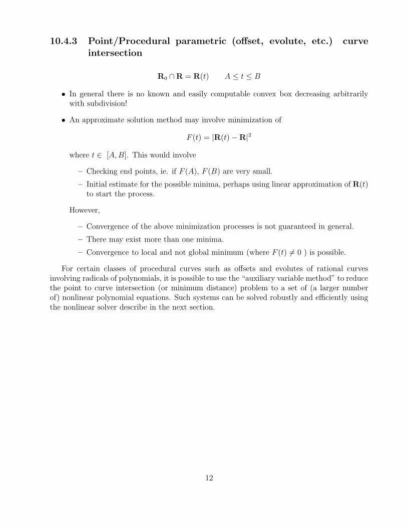
10.4.3 Point/Procedural parametric (offset, evolute, etc.) curveintersection
R0 ∩ R = R(t) A ≤ t ≤ B
• In general there is no known and easily computable convex box decreasing arbitrarilywith subdivision!
• An approximate solution method may involve minimization of
F (t) = |R(t) − R|2
where t ∈ [A,B]. This would involve
– Checking end points, ie. if F (A), F (B) are very small.
– Initial estimate for the possible minima, perhaps using linear approximation of R(t)to start the process.
However,
– Convergence of the above minimization processes is not guaranteed in general.
– There may exist more than one minima.
– Convergence to local and not global minimum (where F (t) 6= 0 ) is possible.
For certain classes of procedural curves such as offsets and evolutes of rational curvesinvolving radicals of polynomials, it is possible to use the “auxiliary variable method” to reducethe point to curve intersection (or minimum distance) problem to a set of (a larger numberof) nonlinear polynomial equations. Such systems can be solved robustly and efficiently usingthe nonlinear solver describe in the next section.
12

10.5 Point/surface intersection
10.5.1 Point/Implicit (usually algebraic) surface intersection
The condition for R0 ∩ {f(R) = 0}, where f(R) = 0 is an implicit surface, is:
|f(R0)| < ε,|f(R0)|
| 5 f(R0)|< δ
where ε, δ are small constants.
10.5.2 Point/Rational polynomial surface intersection
1. Implicitization is possible for all such surfaces but computationally expensive and possi-bly inaccurate. For a tensor product rational polynomial surface with maximum degreesin u and v equal to m and n, of the form
R = R(um, vn),
the implicit equation isf(xq, yq, zq) = 0
where q ≤ 2mn
Therefore, for m = n = 3 −→ q ≤ 18, m = n = 2 −→ q ≤ 8
The above method is useful for special surfaces such as cylindrical and conical ruledsurfaces, surfaces of revolution, etc.
Examples:
(a) Implicitization of a surface of revolution.
y
x
z
r
r
R(t)
Figure 10.7: Surface of revolution.
13
Let us consider a profile curve to be a rational polynomial of degree n, see Figure 10.7
R(t) = [r(t), z(t)]
By simple implicitization of R = R(t), we get:
fn(r, z) = 0 (10.5)
where n is the maximum total degree of f . Also,
r2 = x2 + y2 (10.6)
Next we eliminate r from equations 10.5 - 10.6 by rewriting equations 10.5 - 10.6 asfollows:
fn(r, z) = a0(z)rn + a1(z)r
n−1 + · · ·+ an(z) = 0
⇒ −r2 + (x2 + y2) = 0
The resultant of eliminating r from these two equations is
D =
∣∣∣∣∣∣∣∣∣∣∣∣∣∣∣
a0(z) a1(z) · · · an−1(z) an(z) 00 a0(z) · · · an−2(z) an−1(z) an(z)−1 0 x2 + y2 · · ·
−1 0 x2 + y2
. . .
−1 0 x2 + y2
∣∣∣∣∣∣∣∣∣∣∣∣∣∣∣
= 0
and the degree of D ≡ f(x, y, z) = 0 is 2n. An example is a torus (degree 4 algebraicsurface).
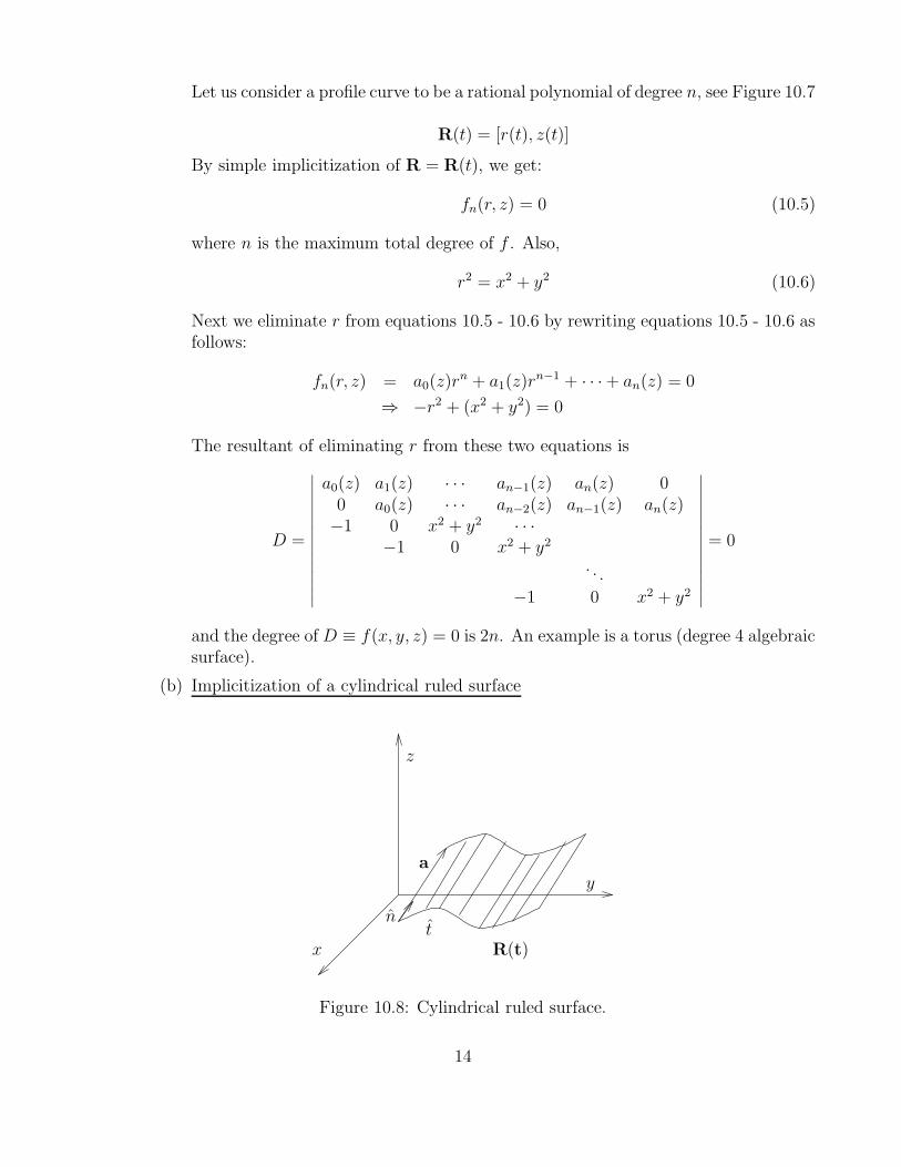
(b) Implicitization of a cylindrical ruled surface
x
y
n
R(t)t
a
z
Figure 10.8: Cylindrical ruled surface.
14

LetR(t) = [X(t), Y (t)]
be a degree n planar rational polynomial curve in the x, y plane. The resultingimplicit equation of the curve
f(X, Y ) = 0
is a polynomial of degree n. Let
a = [a1, a2, a3]
be a direction vector. Then the three equations
x = X + ua1
y = Y + ua2
z = ua3
describe a cylindrical ruled surface. Hence, the implicit surface equation becomes:
f(x− z
a3a1, y −
z
a3a2) = 0
This equation can be transformed to the standard form using a symbolic manipu-lation program such as Macsyma.
(c) Implicitization of a conical ruled surface
x
y
z
R(t)
u
R0
t
Figure 10.9: Conical ruled surface.
LetR0 = [x0, y0, z0]
be the apex of the conical ruled surface and
R(t) = [X(t), Y (t)]
15

a degree n planar rational polynomial curve on the x, y plane. Its implicit equation
f(x, y) = 0
is a degree n polynomial. The equation of the resulting conical ruled surface is
x = x0(1 − u) +Xu
y = y0(1 − u) + Y u
z = z0(1 − u)
Eliminating u = 1 − zz0
and solving for X, Y yields:
f[
z0z0 − z
x− x0
z0 − zz,
z0z0 − z
y − y0
z0 − zz]
= 0
This equation can be transformed to the standard form using a symbolic manipu-lation program such as Macsyma.
2. Newton’s method:Solve x0 = x0(u, v), y0 = y0(u, v) and verify the third equation. Use a linear approxi-mation to start the process. Preprocessing using convex bounding box should always beused, coupled with some level of subdivision.
3. Convex box and possibly subdivision followed by minimization in 0 ≤ u, v ≤ 1 orwithin a rectangular subdomain of the following function (see Figure 10.10).
F (u, v) = |R(u, v)− R0|2 ≥ 0
A point u0, v0 where F (u0, v0) = 0 yields the solution.
u
v
F(u,v)
O
Figure 10.10: Distance function squared
In order to solve this minimization problem, we need to compute
• Minimum of all local minima of F (u, v) (Fu = Fv = 0) in domain;
16

• Minimum of all local minima of boundary “curves” eg. F (0, v) (i.e. Fv = 0);
• Values of F (u, v) at corners, ie. F (0, 0), F (0, 1), F (1, 0), F (1, 1);
and then choose u0, v0 from above solutions where F (u0, v0) = 0.
The disadvantages of a minimization method are:
(a) Initial approximation is required;
(b) Possibility of divergence;
(c) No guarantee that all minima are located. (We need to enhance confidence bysubdivision.)
(d) First and second derivativers of F (u, v) are required.
Note: When R = R(u, v) is a polynomial parametric surface patch, it is helpful toreformulate F (u, v) to
F (u, v) =k∑
i=0
m∑
j=0
wijBi,k(u)Bj,m(n) (10.7)
If wij > 0 for all i, j then there is no solution. We could use wij to construct initialapproximations for the various local minima to be computed by usual descent numericalmethods. These initial approximation may be obtained by discrete sampling or subdivi-sion.
Let F (u, v) be expressed in the Bernstein basis, as in equation (10.7). Then, let us alsoexpress Fu, Fv in the Bernstein basis:
Fu(u, v) =k−1∑
i=0
m∑
j=0
AijBi,k−1(u)Bj,m(v) = 0
Fv(u, v) =k∑
i=0
m−1∑
j=0
BijBi,k(u)Bj,m−1(v) = 0 (10.8)
The equations Fu(u, v) = 0 and Fv(u, v) = 0 represent planar algebraic curves illustratedin Figure 10.11. Their intersection are the required extrema from which the minima can beselected using elementary calculus.
A geometrically motivated solution of the system 10.8 is possible using the convex hullproperty and subdivision to isolate an area where convex hulls intersect.
Taking G(u, v) = Fu(u, v) and n = k − 1 for example, we can write
w = G(u, v) =n∑
i=0
m∑
j=0
AijBi,n(u)Bj,m(v)
We can reformulate this “height” function into a parametric surface as follows:
w = [u, v, G] =∑∑
LijBi,m(u)Bj,n(v)
Lij = [i
m,i
n, Aij]
17

v
Fv = 0
Fu = 0
u 1
1
00
Figure 10.11: Intersection of algebraic curves.
w=0 curve
w=1−u −v2 2= 0
w
u
v
1
Figure 10.12: Control net
To solve Fu = Fv = 0, we find the projection of convex hulls of w(u, v) and of the corre-sponding surface for Fv on the coordinate planes u = 0, v = 0 , then intersect them with thelines w = 0, see Figure 10.12 for an example. A more detailed description of this procedure isgiven in the next section where a nonlinear solver is described.
18

10.5.3 Point/Procedural surface intersection
A procedural surface may be an offset surface or a generalized cylinder surface or a blendingsurface. The typical solution method is minimization. In this case, no convex box assistanceis possible in general, and we need a dense sampling for an initial approximation (which maybe expensive) and no rigorous guarantees for the solution’s reliability are generally available.
For certain classes of procedural surfaces such as offsets and evolutes of rational surfacesinvolving radicals of polynomials, it is possible to use the “auxiliary variable method” to reducethe point to surface intersection (or minimum distance) problem to a set of (a larger numberof) nonlinear polynomial equations. Such systems can be solved robustly and efficiently usingthe nonlinear solver describe in the next section.
19

10.6 Curve/curve intersection
The curve types we will consider can be classified as follows:
• Rational polynomial parametric (RPP)
• Procedural parametric (PP)
• Implicit algebraic (IA)
• Implicit procedural (IP)
Procedural curves may be general offsets, evolutes, etc.Curve to curve intersection cases are identified in table 10.1.
RPP PP IA IPRPP D1 D2 D3 D4PP D5 D6 D7IA D8 D9IP D10
Table 10.1: Curve to curve intersection cases
Conceptually, D3 (RPP/IA curve intersection) is the “simplest” of the above cases of inter-section to describe and use for illustrating various general difficulties of intersection problems.
10.6.1 Case D3: RPP/IA curve intersection
We start with a planar RPP curve (which is conceptually the simplest case).
R(t) = [x(t), y(t)] = [X(t)
w(t),Y (t)
w(t)]
=
∑ni=0 RihiBi,n(t)∑n
i=0 hiBi,n(t)0 ≤ t ≤ 1
where hi > 0 are weights and Bi,n(t) are Bernstein basis functions.The implicit algebraic curve fm(x, y) = 0 of total degree m is described by
fm(x, y) =m∑
i=0
m−i∑
j=0
cijxiyj = 0
For convenience, we convert it to homogeneous form, by setting x = Xw
, y = Yw
and multiplyingby wm, which leads to
fm(X, Y, w) =m∑
i=0
m−i∑
j=0
cijXiY jwm−i−j = 0
20

Every term of the above sum has a total degree m. Substituting R(t) into fm(X, Y, w) leadsto a polynomial of degree up to mn
F (t) = 0
Therefore, now the problem of intersection is equivalent to finding the real roots of F (t) in0 ≤ t ≤ 1. The most usual form of F (t) is the power basis. The coefficients ai can be evaluatedsymbolically by substitution and collection of terms. This can be readily done in a standardsymbolic manipulation program (such as Macsyma, Reduce, Maple etc.). Such programs areoriented to processing rational numbers exactly.
Example:
Let the algebraic curve be an ellipse x2
4+ y2 − 1 = 0, as illustrated in Figure 10.13. Let the
parametric curve be a cubic Bezier curve with control points:
[
01
]
,
[
1−4
]
,
[
21
]
, and
[
20
]
x
y
1
2
Figure 10.13: Ellipse and cubic Bezier curve polygon
Using Macsyma (or any similar symbolic manipulation program) and simplifying, we get(in exact arithmetic mode):
F (t) = 1025t6 − 3840t5 + 5514t4 − 3728t3 + 1149t2 − 120t = 0
Next we find the (real) roots of F (t) in t ∈ [0, 1] using Macsyma’s factoring capability overintegers, which leads to
F (t) ≡ t(t− 1)2G(t)
whereG(t) = [1025t3 − 1790t2 + 909t− 120]
21

Using a standard numerical solver for polynomials in floating point (such as NAG C02AEFroutine), we obtain the following numbers as solutions of G(t) = 0 (reported with four decimaldigits)
t = 0.9228, 0.61843, 0.2051
Alternately solving F (t) = 0 using the same routine leads to the following roots t = tR + itI
tR 1 1 0.9228 0.6183 0.2051 0tI −0.22 × 10⁻⁶ 0.22 × 10⁻⁶ 0 0 0 0
Notice the sensitivity to errors for the 6th degree polynomial, especially for multiple rootsas t = 1. In floating point arithmetic, such roots split into a number of roots (complex or real).Obviously, complex roots are not usable (as we require only the real intersection points). Theconsequence is lost roots, which implies an erroneous solution of the intersection problem.
An alternate basis for the representation of F (t) = 0 is the Bernstein basis, which has betterstability of its real roots under perturbations of its coefficients than the power form. We willintroduce the concept of condition numbers for polynomial roots later in this subsection.Suchrepresentation can be obtained without first converting to a power basis and using a symbolicmanipulation program. It rather requires polynomial arithmetic involving products such as
Bi,k(t)Bj,l(t) =
(
ki
)(
lj
)(
k + li+ j
)−1
Bi+j,k+l(t)
In this way we obtain the representation:
F (t) =mn∑
i=0
ciBi,mn(t) = 0
In the above example of the ellipse and cubic Bezier curve,
c0 = 0, c1 = −20, c2 = 36.6, c3 = −16.6, c4 = 1.6, c5 = 0, and c6 = 0
Using the linear precision property
t =mn∑
i=0
i
mnBi,mn(t)
we can construct
f(t) = [t, F (t)] =mn∑
i=0
(i
mn
ci
)
Bi,mn(t)
which is now a standard degree mn Bezier curve as in Figure 10.14Notice that in our example c0 = 0 which implies that t = 0 is a root. Also c5 = c6 = 0
implies that t = 1 is a double root. Note that
• If all ci > 0 or ci < 0 then there are not roots in [0, 1].
• We can use subdivision (split in half) to identify subintervals of [0, 1] where coefficientschange sign once. Variation diminishing property implies one root in such areas. TheNewton method can be used for fast convergence within such subintervals.
22

15
30
45
−15
−30
−45
1/6
2/6 3/6 4/6 5/6 1 t0
0.21
0.610.92
Figure 10.14: Intersection of a Bezier curve/straight line.
Another solution method is illustrated in Figure 10.15 for a quadratic curve (parabola). In thismethod the curve’s convex hull is intersected with the axis w = 0 to give the [A,B] intervalas in Figure 10.15. The part of the [0, 1] interval outside [A,B] does not contain roots. Bycurve subdivision at A and B a smaller curve segment can be obtained in the Bezier form andthe process can be continued. In this case, we use binary subdivision of AB when the rate ofdecrease of AB slows. See paper by Sherbrooke and Patrikalakis for details and also the nextsection on the nonlinear solver.
0 1A B
w
w = 0
Figure 10.15: Subdivision at A, B.
Numerical condition of polynomials in Bernstein form
1. Condition numbers for polynomial rootsConsider the displacement δx of a real root xo of a polynomial in the basis {φk(x)}:
P (x) =n∑
k=0
λkφk(x),
23

due to a perturbation δλr in a single coefficient λr in this basis. Since xo + δx is a rootof the perturbed polynomial, it satisfies:
P (xo + δx) = −δλrφr(xo + δx).
Performing a Taylor series expansion about xo on both sides of the above equation andnoting that P (xo) = 0, we obtain:
n∑
k=1
(δx)k
k!P (k)(xo) = −δλr
n∑
k=0
(δx)k
k!φ(k)
r (xo).
If xo is a simple root of P (x), then P ′(xo) 6= 0, and in the limit of infinitesimal pertur-bations the above equation gives:
limδλr→0
δx
δλr/λr
= −λrφr(xo)
P ′(xo).
We defineC = |λrφr(xo)/P
′(xo)|the condition number of the root xo with respect to the single coefficient λr.
If xo is an m-fold root, m ≥ 2, then we define a multiple-root condition number C (m) inthe form
C(m) = [m!
|P (m)(xo)|n∑
r=0
|λrφr(xo)|]1/m.
Theorem For an arbitrary polynomial P (x) with a simple root xo ∈ [0, 1], let Cp(xo) andCb(xo) denote the condition numbers of the root in the power and Bernstein bases on [0, 1],respectively. Then Cb(xo) ≤ Cp(xo) for all xo ∈ [0, 1]. In particular Cb(0) = Cp(0) = 0,while for xo ∈ (0, 1] we have the strict inequality Cb(xo) < Cp(xo).
2. Example – Wilkinson polynomial
Consider the polynomial with the linear distribution of real roots xo = k/n, k = 1, 2, ..., n,on the unit interval [0, 1] for n = 20:
P (x) =20∏
k=1
(x− k/20).
The condition numbers for each root with respect to a perturbation in the single co-efficient a19 are shown in Table 10.2. It is evident from Table 10.2 that the Bernsteinform affords a dramatic inprovement in root condition numbers compared to the powerform in this example, the condition number of the most unstable root being reduced bya factor of about 107.
We now perturb the single power coefficient a19 = −212
by an amount −2−23/20. Thiscorresponds to a fractional perturbation ε = 2−23/210 ∼= 5.7 × 10⁻¹⁰. The roots of the
24

Table 10.2: Condition numbers for Wilkinson polynomial
k Cp(xo) Cb(xo)1 2.100 × 101 3.413 × 100
2 4.389 × 10³ 1.453 × 10²
3 3.028 × 10⁵ 2.335 × 10³
4 1.030 × 10⁷ 2.030 × 10⁴
5 2.059 × 10⁸ 1.111 × 10⁵
6 2.667 × 10⁹ 4.153 × 10⁵
7 2.409 × 10¹⁰ 1.115 × 10⁶
8 1.566 × 10¹¹ 2.215 × 10⁶
9 7.570 × 10¹¹ 3.321 × 10⁶
10 2.775 × 10¹² 3.797 × 10⁶
11 7.822 × 10¹² 3.321 × 10⁶
12 1.707 × 10¹³ 2.215 × 10⁶
13 2.888 × 10¹³ 1.115 × 10⁶
14 3.777 × 10¹³ 4.153 × 10⁵
15 3.777 × 10¹³ 1.111 × 10⁵
16 2.833 × 10¹³ 2.030 × 10⁴
17 1.541 × 10¹³ 2.335 × 10³
18 5.742 × 10¹² 1.453 × 10²
19 1.310 × 10¹² 3.413 × 100
20 1.378 × 10¹¹ 0
25

pertured polynomials are shown in Table 10.3. For comparison, we now perturb thecoefficient
c19 = − 14849255421
12800000000000000000of the Bernstein form by the same fractional amount, and obtain approximations to theroots of this perturbed polynomial, which are shown in Table 10.3.
Table 10.3: Roots of perturbed polynomials
k power Bernstein1 0.05000000 0.05000000002 0.10000000 0.10000000003 0.15000000 0.15000000004 0.20000000 0.20000000005 0.25000000 0.25000000006 0.30000035 0.30000000007 0.34998486 0.35000000008 0.40036338 0.40000000009 0.44586251 0.450000000010 0.50476331± 0.500000000011 0.03217504i 0.549999999712 0.58968169± 0.600000001013 0.08261649i 0.649999997214 0.69961791± 0.700000005315 0.12594150i 0.749999993016 0.83653687± 0.800000006317 0.14063124i 0.849999996218 0.97512197± 0.900000001319 0.09701652i 0.949999999820 1.04234541 1.0000000000
3D-Space geometry: Case D3: RPP/IA (continued)
R(t) = [x(t), y(t), z(t)] ∩ f(R) = g(R) = 0
1. Substitute
f(R(t)) ≡ F1(t) = 0
g(R(t)) ≡ F2(t) = 0
2. Compute the resultant of F1(t), F2(t) by eliminating t.
3. If R(F1(t), F2(t)) ≡ 0, then there is a common root between the two equations.
4. Use the inversion algorithm to find t.
26

10.6.2 Case D1: RPP/RPP Curve Intersection
{
R1 = R1(t), 0 ≤ t ≤ 1R2 = R2(v), 0 ≤ v ≤ 1
Setting R1(t) = R2(v) leads to 3 nonlinear equations with 2 unknowns (overdeterminedsystem). A possible approach is to choose 2 equations to solve for t, v, and then substitute theresults into the third equation for verification. Alternatively the subdivision-based nonlinearsolver described in the next section can directly solve such systems without the above 2 stepapproach.
Preprocessing idea in 3D:Check bounding boxes for intersection. If there is such intersection, examine x, y projection.
Method 1 .
1. Implicitize, e.g., x2 = x2(v), y2 = y2(v), to get f(x, y) = 0.
2. Substitute x1(t), y1(t) into f(x, y) to get F (t) = 0 and solve it for real roots in [0, 1].
3. Use the inversion algorithm: v = φ(x,y)q(x,y)
Method 2 Recursive subdivision and use of bounding boxes.
Some issues:
Method 1 is more efficient for n ≤ 3 but its robustness is unclear in the presence of ill-conditioned (tangent) intersections.
Method 2 is more efficient for n ≥ 4 and its robustness with respect to missing roots canbe guaranteed if the method is inplemented in rounded interval arithmetic (see nextsection). If two bounding boxes intersect, and they are of finite size, we can find rootsusing linear approximation.
In Figure 10.16(a), the boxes intersect, the linear approximation do not, and the curvesintersect. Similar behavior is observed in (b) where polygon is used as the curve approx-imation.
(a) (b)
Figure 10.16: Ill-conditioned curve intersections.
27
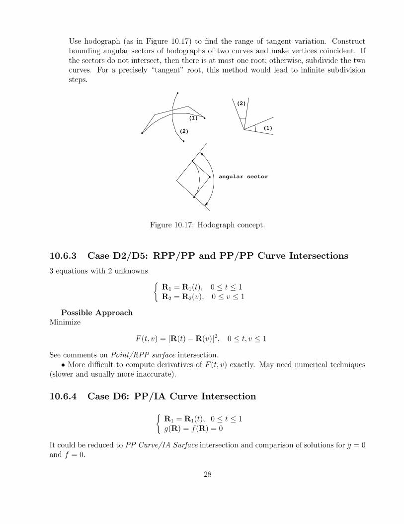
Use hodograph (as in Figure 10.17) to find the range of tangent variation. Constructbounding angular sectors of hodographs of two curves and make vertices coincident. Ifthe sectors do not intersect, then there is at most one root; otherwise, subdivide the twocurves. For a precisely “tangent” root, this method would lead to infinite subdivisionsteps.
(1)
(2)(1)
(2)
angular sector
Figure 10.17: Hodograph concept.
10.6.3 Case D2/D5: RPP/PP and PP/PP Curve Intersections
3 equations with 2 unknowns{
R1 = R1(t), 0 ≤ t ≤ 1R2 = R2(v), 0 ≤ v ≤ 1
Possible ApproachMinimize
F (t, v) = |R(t) − R(v)|2, 0 ≤ t, v ≤ 1
See comments on Point/RPP surface intersection.• More difficult to compute derivatives of F (t, v) exactly. May need numerical techniques
(slower and usually more inaccurate).
10.6.4 Case D6: PP/IA Curve Intersection
{
R1 = R1(t), 0 ≤ t ≤ 1g(R) = f(R) = 0
It could be reduced to PP Curve/IA Surface intersection and comparison of solutions for g = 0and f = 0.
28

10.6.5 Case D8: IA/IA Curve Intersection
The planar case is of interest in processing trimmed patches.
f(u, v) = 0g(u, v) = 0
}
(u, v) ∈ Parametric domain
Method 1Eliminate v to form the resultant F (u), then solve F (u) = 0 for u and use the inversionalgorithm to get v.• Example: Let us consider an ellipse and a circle
f =x2
4+ y2 − 1 = 0
g = (x− 1)2 + y2 − 1 = 0
as in Figure 10.18.
x
y
Figure 10.18: Ellipse and circle intersection
Let us eliminate y from these two equations. This leads to
3x2 − 8x+ 4 = 0
which has as roots x = 2 and x = 23. Each of these leads to y2 = 0 and y2 = 8
9respectively.
However there are possible numerical problems at the “tangent” solution x = 2, y = 0.Let us assume that due to error
x = 2 + ε
hencey2 = −ε(1 +
ε
4) < 0
This implies that y is imaginary and that no real roots exist. This would have as aconsequence missing an intersection solution, leading to a robustness problem.
Method 2After tracing of f(u, v) = 0 and g(u, v) = 0, linear approximation is available. Findintersections of linear approximations and minimum distance points between them. Usethis to drive a Newton Method on f = g = 0 or a minimization of F = f 2 + g2.
29
10.7 Curve/surface intersection
Such intersections are classified as in Table 10.4. We will start with case E3 which is quiterepresentative.
Surface TypeCurve Type RPP PP IA IP
RPP E1 E2 E3 E4PP E5 E6 E7 E8IA E9 E10 E11 E12IP E13 E14 E15 E16
Table 10.4: Curve/Surface Intersections
Curve to surface intersection involves the intersection of straight line to surface of all cases.Such intersection is useful for
• ray tracing
• point classification
• for procedural surface interrogation
10.7.1 Case E3: RPP Curve/IA Surface Intersection
Let us consider an (implicit) algebraic surface of total degree m
fm(x, y, z) =m∑
i=0
m−i∑
j=0
m−i−j∑
k=0
cijkxiyjzk = 0
We first convert it to a degree homogeneous form by setting x = X/W, y = Y/W, z = Z/Wand multiply by Wm leading to
fm(X, Y, Z,W ) =m∑
i,j,k,q=0i+j+k+q=m
cijkXiY jZkW q = 0
Let us also consider a rational curve of degree n
R(t) = [x(t), y(t), z(t)] = [X(t)
W (t),Y (t)
W (t),Z(t)
W (t)], 0 ≤ t ≤ 1
We can easily substitute R(t) in fm(X, Y, Z,W ) to obtain a polynomial equation F (t) = 0 ofdegree ≤ mn. We then find its (real) roots in [0, 1], see comments under section 10.6.1.
30

10.7.2 Case E1: RPP Curve/RPP Surface Intersection
3 nonlinear equations in 3 unknowns t, u, v,R(t) = Q(u, v) where
R = R(t), 0 ≤ t ≤ 1Q = Q(u, v), 0 ≤ u, v ≤ 1
A Preprocessing step is to check bounding boxes for absence of intersection to eliminateeasy cases.
Method 1 Implicitization of Q(u, v) for simple surface forms and reduction to Case E3.
Method 2 Recursive subdivision and use of bounding boxes. See also next section for nonlin-ear solver. Eventual use of a linear approximation technique for R and Q to obtain ap-proximate solution, which is to be used to initiate a Newton method on R(t)−Q(u, v) = 0or a minimization method on F (t, u, v) = |R−Q|2. See section 10.6.2 for problem areasfor Ft = Fu = Fv = 0 (3 equations.)
10.7.3 Case E2/E6: RPP/PP, PP/PP Curve/Surface Intersection
3 nonlinear equations in 3 unknowns t, u, v,R(t) = Q(u, v) where
{
R = R(t), 0 ≤ t ≤ 1 ∩Q = Q(u, v), 0 ≤ u, v ≤ 1
Possible ApproachMinimize
F (t, u, v) = |R(t) − Q(u, v)|2
in a cube 0 ≤ t, u, v ≤ 1. See comments under point-surface intersection (e.g. examine vertices,edges, etc.)
10.7.4 Case E7: PP Curve/IA Surface Intersection
4 non-linear equations in 4 unknowns t,R
{
R = R(t), 0 ≤ t ≤ 1f(R) = 0
Possible approachCould use a Newton method initiated by a linear approximation of R = R(t), which can beintersected more easily with f(R) = 0 using the method of Case E3.
Problems
1. All roots?
2. Convergence?
31

3. Efficiency?
In case of convergence problems, embedding or continuation methods are normally helpful.For example,
1. Let
Q(t) = Q0 + (Q1 − Q0)t− a
b− a, t ∈ [a, b]
where [a, b] ⊂ [0, 1], be an approximation of R(t) within [a, b] interval.
2. Compute Q(t) ∩ f(R) = 0 in t ∈ [a, b] using the method of Case E3.
3. Define sequence of problems
R(t; ε) = Q(t) + ε(R(t) − Q(t))
where ε = ε1, ε2, · · · , εN such that 0 = ε1 < ε2 < · · · < εN = 1.
4. Solve R(t; εi) ∩ f(R) = 0 using as initial approximation the solution for ε = εi−1.
Such a method does not by itself provide initial approximations of all possible solutions; rather,it assists in the computation of a particular solution.
10.7.5 Case E11: IA Curve/IA Surface Intersection
3 equations in 3 unknowns
f(R) = g(R)︸ ︷︷ ︸
curve
= h(R)︸ ︷︷ ︸
surface
= 0
Possible approaches
1. Elimination Methods
2. Newton Methods
3. Minimization Methods
F (R) = f 2 + g2 + h2
Possible reformulation in a box Π
F (R) =M∑
i=0
N∑
j=0
Q∑
k=0
wijkBi,M(x)Bj,N(y)Bk,Q(z)
(x, y, z) ∈ Π = [a1, a2] × [b1, b2] × [c1, c2]
and x = (x− a1)/(a2 − a1) and similarly for y and z. If wijk > 0 for all i, j, k, there is nosolution is Π.
Initial approximation: find mini,j,kwijk < 0 and start at ( iM, j
N, k
Q).
4. Approximate f(R) = g(R) = 0 curve with a linear spline, reduce to E3 and refine usingminimization.
32

10.7.6 IA Curve/RPP Surface Intersection
{
curve f(R) = g(R) = 0surface R = R(u, v), 0 ≤ u, v ≤ 1
Substitute R = R(u, v) in f(R) = 0, g(R) = 0 to obtain two algebraic curves f(u, v) =0, g(u, v) = 0, as in Figure 10.19. This formulation reduces to Case D8 in Section 10.6.5:IA/IA curve intersection. Algebraic curves are treated under intersections of algebraic andRPP surfaces.
f=0g=0
u
v
Figure 10.19: Intersection of two algebraic curves
33
10.8 Surface/Surface Intersections
The surface types we will consider can be classified as follows:
• Rational polynomial parametric (RPP)
• Procedural parametric (PP)
• Implicit algebraic (IA)
• Implicit procedural (IP)
Procedural surfaces may include general offsets, focal surfaces, etc.Surface to surface intersection cases are identified in table 10.5.
Surface TypeSurface Type RPP PP IA IP
RPP F1 F2 F3 F4PP F5 F6 F7IA F8 F9IP F10
Table 10.5: Classification of Surface/Surface Intersections
The solution of a surface/surface intersection problem may be empty, or include a curve(possibly made of several branches), a surface patch, or a point. Conceptually, F3 (RPP/IAsurface intersection) is the “simplest” of the above cases of intersection to describe and use forillustrating general difficulties of surface intersection problems.
10.8.1 Case F3: RPP/IA Surface Intersection
We start with a RPP surface patch
R(u, v) = [X(u, v)
W (u, v),Y (u, v)
W (u, v),Z(u, v)
W (u, v)] (10.9)
where X, Y, Z are all of degree p in u, q in v, (u, v) ∈ [0, 1] × [0, 1].Next we consider an implicit algebraic surface fm(x, y, z) = 0 of total degree m described
by
fm(x, y, z) =m∑
i=0
m−i∑
j=0
m−i−j∑
k=0
cijkxiyjzk (10.10)
Examples of such surfaces in practical use are low order surfaces such as planes (degree 1), thenatural quadrics (cylinder, sphere, cone) (degree 2), and torii (degree 4). In fact in a survey ofmechanical parts (mechanical elements), over 90% of all surfaces involved are of these types. Itis also well known that all these surfaces also have a low degree rational polynomial parametric
34

representation, so that when two surfaces of the above types are intersected, the methods ofthis section may be used.
For convenience, we convert fm(x, y, z) = 0 to its homogeneous form by setting
x =X
W, y =
Y
W, z =
Z
W(10.11)
and multiplying by Wm, which leads to
fm(X, Y, Z,W ) =∑
i, j, k, q ≥ 0i + j + k + q = m
cijkXiY jZkW q = 0 (10.12)
Consequently, the intersection problem
fm(X, Y, Z,W ) = 0 (10.13)
X = X(u, v), Y = Y (u, v), Z = Z(u, v), W = W (u, v) (10.14)
may be thought of as a nonlinear system of 5 equations in 6 unknowns. A reduction of the di-mensionality of the system may be obtained by substituting equations 10.14 in equation 10.13,which since all functions involved are polynomial leads to an algebraic curve
f(u, v) = 0 (10.15)
of degree M = mp and N = mq in u, v, respectively. Consequently, the problem of intersectionreduces to the problem of tracing f(u, v) = 0 without omitting any special features of the curve,e.g., small loops, singularities, and accurately computing all its branches. This is a fundamentalproblem in algebraic geometry and much work has been done to understand its solution. In thecontext of algebraic geometry the coefficients of f(u, v) = 0 are integers. In the context of CADand computer implementation, the coeffficients of fm = 0, and R = R(u, v) are floating pointnumbers. Consequently, if the above substitution is performed in floating point arithmetic thecoefficients of f(u, v) = 0 involve error. To avoid such error, rational arithmetic may be usedfor robustness. These issues will also be discussed in the next section.
The algebraic curve
f(u, v) =M∑
i=0
N∑
j=0
aijuivj = 0 (10.16)
can be reformulated as
f(u, v) =M∑
i=0
N∑
j=0
wijBi,M(u)Bj,N(v) = 0 (10.17)
where (u, v) ∈ [0, 1]2.As an example consider a plane in homogeneous form
AX +BY + CZ +DW = 0 (10.18)
35

u
v
1
1
borderpoints singular
points
loop
Figure 10.20: Parameter space of R(u, v) and resulting algebraic curve f(u, v) = 0
and a rational Bezier patch of degree p in u, q in v
R(u, v) =
∑pi=0
∑qj=0 hijRijBi,p(u)Bj,q(v)
∑pi=0
∑qj=0 hijBi,p(u)Bj,q(v)
(10.19)
where Rij = [xij, yij, zij] and weights hij ≥ 0.The resulting algebraic curve is of the form of equation 10.17 with
wij = (Axij +Byij + Czij +D)hij (10.20)
In fact the power basis form of f(u, v) = 0 need not be computed at all, if polynomial arithmeticfor Bernstein polynomials is used.
The advantage of the Bernstein form is its numerical stability and convex hull property.If wij > 0 or < 0 for all i, j, there is no solution and the two surfaces do not intersect.More precisely, the (entire) algebraic surface fm(R) = 0 does not intersect the surface patchR = R(u, v) for (u, v) ∈ [0, 1]2.
What happens when all wij = 0 (or αij = 0)? Obviously, the two surfaces coincide intheir entirety. A somewhat complex algebraic curve f(u, v) = 0 is shown in Figure 10.20involving various branches (from border to border), internal loops, and singularities, see alsoFigure 10.24.
Given a point on every branch (connected component) of an algebraic curve, tracing thecurve using differential curve properties is an effective procedure (marching method).
Marching Method:
Let us expand f(u, v) as a Taylor series
36

δvLδv
δu
(u,v)
Newton
Figure 10.21: A zoomed view of an algebraic curve near a point (u, v)
f(u+ δu, v + δv) = f(u, v) + fuδu+ fvδv
+1
2(fuuδu
2 + 2fuvδuδv + fvvδv2) + · · · (10.21)
- To first order and if f 2u + f 2
v > 0, in order to have f(u, v) = 0 and f(u+ δu, v + δv) = 0,
fuδu+ fvδvL = 0 ⇒ δvL = −fu
fvδu (10.22)
see also Figure 10.21.
- The Newton method on f(u + δu, v) = 0 with initial approximation vI = v + δvL may beused to compute vF = v + δv with high accuracy and in an efficient manner.
- For “vertical” branches, ie. when |fv| is very small, we may use δuL = − fv
fuδv.
To avoid these special stepping procedures the equation fuδu+ fvδv = 0 may be convertedto
fuu+ fv v = 0 (10.23)
where u, v are considered functions of a parameter t, u = u(t), v = v(t). This equation issatisfied if
u = −ξfv(u, v) (10.24)
v = ξfu(u, v) (10.25)
where ξ is an arbitrary constant. For example, ξ can be chosen to be equal to [f 2u + f 2
v ]−12 , in
order that t is an arc length parameter in the [u, v] ∈ [0, 1]2 parameter space. This is a system
37

of two first order nonlinear differential equations which can be solved by the Runge-Kutta orother methods with adaptive step size.
Problems of Marching Methods
1. Starting points on all branches need to be provided in advance.
2. Marching through singularities (f 2u + f 2
v ' 0) is problematic.
3. Step size selection is complex and too large a step size may lead to straying or looping,as in Figure 10.22.
straying looping
Figure 10.22: Step size problems in marching method
Computation of starting points
Starting points for tracing algebraic curves are certain “characteristic” points defined below:
1. Border points, ie. the intersections of f(u, v) = 0 with the boundary of the parameterspace [0, 1]2, e.g., f(0, v) = 0, 0 ≤ v ≤ 1.
2. Turning points f = fu = 0 or f = fv = 0, which are illustrated in Figure 10.23. If f is ofdegree (M,N) in (u, v), then fu is of degree (M−1, N) and fv is of degree (M,N−1). Itcan be seen that the total number of roots of two simultaneous bivariate polynomials ofdegree (m,n) and (p, q), respectively, is mq + np.Thus, there can be at most 2MN −Mu-turning points and 2MN −N v-turning points.
3. Singular points f = fu = fv = 0. Notice fu = ∇f · Ru, fv = ∇f · Rv, and thereforefu = fv = 0 means that ∇f ‖ Ru × Rv or that the normals of two surfaces are paralleland since f(u, v) = 0 at these points the two surfaces intersect tangentially. If f is ofdegree (M,N) in (u, v), fu is of degree (M − 1, N) and fv is of degree (M,N − 1), therecan be at most 2MN −M −N + 1 singular points.
38

f = fu = 0 f = f = 0v
Figure 10.23: Turning points
From the above discussions we can get upper bounds for the maximum number of u-turning,v-turning and singular points, see table 10.6. These bounds refer to the maximum possiblenumber of solutions (u, v) in the entire complex plane. It turns out that the number of suchpoints in the real square [0, 1]2 is much smaller, but still quite large. Consequently methodswhich focus on the possible solutions only in the [0, 1]2 are advantageous. The subdivisionmethod of Section 10 is one such method. Interval Newton methods are also potentially usefulin this context.
algebraic curve max number max number max numberS1 S2 f(u, v) degree u-turning pts v-turning pts singular points
M,N 2MN −M 2MN −N 2MN −M −N + 1plane biquadratic 2, 2 6 6 5plane bicubic 3, 3 15 15 13
quadric biquadratic 4, 4 28 28 25quadric bicubic 6, 6 66 66 61torus biquadratic 8, 8 120 120 113torus bicubic 12, 12 276 276 265
biquadratic biquadratic 16, 16 496 496 481bicubic biquadratic 36, 36 2556 2556 2521bicubic bicubic 54, 54 5778 5778 5725
Table 10.6: Number of turning and singular points in various cases
Analysis of singular points:
Let (u0, v0) satisfy f(u0, v0) = 0. We construct a straight line L
u = u0 + αt, v = v0 + βt (10.26)
and we find its intersections with the algebraic curve f(u, v) = 0 by substitution as follows:
0 = f(u0 + αt, v0 + βt)
= f(u0, v0) + αtfu(u0, v0) + βtfv(u0, v0)
+1
2(α2t2fuu + 2αβt2fuv + β2t2fvv)|(u=u0,v=v0)
39

+h.o.t. (up to tλ, λ is finite)
= t(αfu + βfv) +t2
2(α2fuu + 2αβfuv + β2fvv) + h.o.t. (10.27)
(1) Case A: f 2u + f 2
v > 0, f = 0 at (u0, v0).
L is tangent to f = 0 at (u0, v0) if t = 0 is a double root. Thus
αfu + βfv = 0
α = ∓fv
β = ±fu
This is also a proof of fact that ∇f is ⊥ to curve.
(2) Case B: fu = fv = f = 0 at (u0, v0).
t = 0 is a triple root if f 2uu + f 2
uv + f 2vv > 0 and at least one of the 3rd derivatives is
nonzero and
α2fuu + 2αβfuv + β2fvv|u=u0v=v0
= 0 (10.28)
We can solve this quadratic equation for αβ
or βα
and there are three possiblities:
(1) 2 real distinct roots ⇒ 2 distinct tangents (self-intersection)
(2) 1 real double root ⇒ 1 tangent (cusp)
(3) 2 complex roots ⇒ no real tangents (isolated point)
See also Figure 10.24 for illustration of the three cases.
Example 1: Let f(u, v) = u3 + u2 + v2 = 0 so that
fu = u(3u+ 2), fv = 2v, fuu = 6u+ 2, fvv = 2, fuv = 0
Turning points:
(1) f = fu = 0, fv 6= 0 ⇒ u = −2
3f = 0 ⇒ v2 = −u2(1 + u) < 0 ⇒ no real solution
(2) f = fv = 0, fu 6= 0 ⇒ v = 0, u = −1
Singular points:
f = fu = fv = 0 ⇒ u = v = 0
Tangents at u = v = 0 can be obtained from 2α2 + 2β2 = 0, (αβ)2 + 1 = 0, which has no real
solution, so u = v = 0 is an isolated point.
40
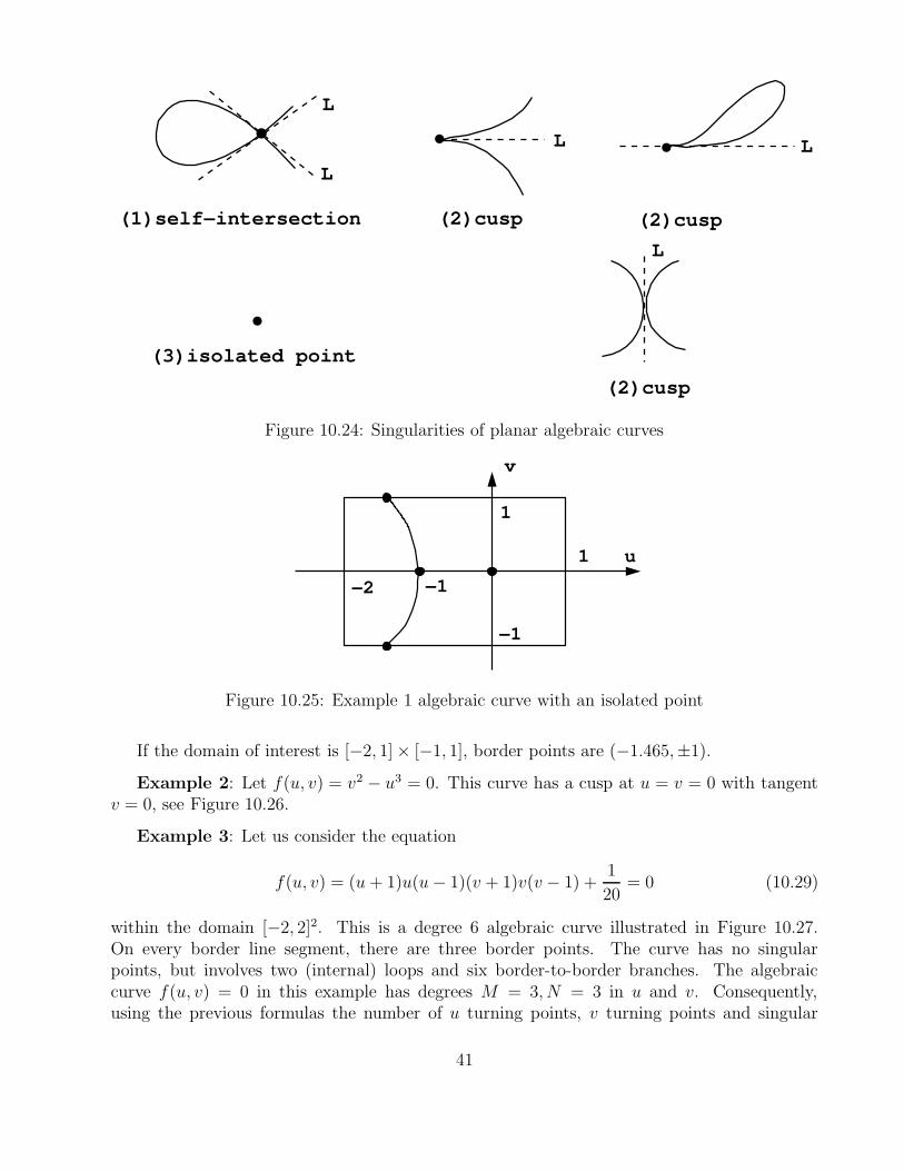
(1)self−intersectio n (2)cusp (2)cusp
(3)isolated point
(2)cusp
L
L
L L
L
Figure 10.24: Singularities of planar algebraic curves
u
v
1
1
−1
−1
−2
Figure 10.25: Example 1 algebraic curve with an isolated point
If the domain of interest is [−2, 1] × [−1, 1], border points are (−1.465,±1).
Example 2: Let f(u, v) = v2 − u3 = 0. This curve has a cusp at u = v = 0 with tangentv = 0, see Figure 10.26.
Example 3: Let us consider the equation
f(u, v) = (u+ 1)u(u− 1)(v + 1)v(v − 1) +1
20= 0 (10.29)
within the domain [−2, 2]2. This is a degree 6 algebraic curve illustrated in Figure 10.27.On every border line segment, there are three border points. The curve has no singularpoints, but involves two (internal) loops and six border-to-border branches. The algebraiccurve f(u, v) = 0 in this example has degrees M = 3, N = 3 in u and v. Consequently,using the previous formulas the number of u turning points, v turning points and singular
41

−1 1
1
−1
u
v
Figure 10.26: Example 2 algebraic curve with a cusp at (u, v) = (0, 0)
points (in the entire complex plane) is bounded by 2MN −M = 15, 2MN − N = 15, and2MN − M − N + 1 = 13. However, as we can be seen in Figure 10.27, these numbersoverestimate the actual number of such points in the real square [−2, 2]2.
Computing starting points for all branches
1. Border points: This involves solution of a polynomial, eg.
f(0, v) =N∑
j=0
w0jBj,N(v) = 0
A robust and efficient solution of this type of equation is addressed in Section 10.
2. Turning and singular point computation: Here we use the fact that
fu(u, v) = MM−1∑
i=0
N∑
j=0
(wi+1,j − wij)Bi,M−1(u)Bj,N(v) (10.30)
fv(u, v) = NM∑
i=0
N−1∑
j=0
(wi,j+1 − wij)Bi,M(u)Bj,N−1(v) (10.31)
Consequently, computing turning points (f = fu = 0 and f = fv = 0) is equivalent tosolving a system of two nonlinear polynomial equations in two variables, and computingsingularities f = fu = fv = 0 is equivalent to solving a system of three nonlinearpolynomial equations in two variables. Robust and efficient solution of these systems ofnonlinear polynomial equations is addressed in Section 10.
10.8.2 Case F1: RPP/RPP Surface Intersection
In this case we have two rational polynomial surface patches{
R1 = R1(u, v)R2 = R2(s, t)
(10.32)
42

2
2
−2
−2
Figure 10.27: Example 3 algebraic curve
eg. two rational Bezier patches and by setting R1 = R2 we obtain three nonlinear polynomialequations for four unknowns u, v, s, t. This system can be solved by the nonlinear solver ofSection 10. However, as the solutions are typically not isolated points but curves, such approachis inefficient. There are three major techniques for solving RPR/RPP surface intersections.
Method 1: Lattice methodIn this method, one of the two surface patches is discretized to a grid of isoparametercurves at some fixed resolution. Each of the resulting curves is intersected with the otherpatch (using a technique as in Section 9.7). The resulting solution points are connectedto form various curve branches based on empirical distance-based criteria. The methodis typically inefficient (because it does not use the convex hull properties of RPP surfacepatches to their full extent) and generally not robust, leading to missing of small featuresof the intersection such as small loops, singularities. Also the connection of the pointsto form curves near constrictions and singularities is not robust as it is empirical.
Method 2: Subdivision methodTypically, subdivision methods involve the follwing steps, see Figure 10.28,
• Preprocessing by bounding boxes to eliminate subpatches that do not intersect.
• Subdivision (typically in four subpatches by multiple knot insertion at the mid pointof parameter axes in NURBS patches)
43

• Approximation of the surface with triangular facets (either from the polyhedron ora grid on the subdivided surface)
• Intersections of triangular facets.
Quadtree
Figure 10.28: Subdivision method
Issues:
- Robust: resolution of loops and isolated points (under finite subdivision) is not guar-anteed.
- Efficiency is typically better than lattice methods but usually inferior to marchingmethods.
Method 3: Marching along tangent to intersection curve
t = (R1u × R1v) × (R2s × R2t) (10.33)
Issues:
- Finding starting points on all branches.
- Straying, looping, singularities
44

u
v
s
t
Figure 10.29: Parameter spaces of R1(u, v) and R2(s, t)
Let us consider the intersection, R1(u, v) = R2(s, t), eg. as illustrated in the parameterspaces of R1, R2 in Figure 10.29. A resulting intersection curve branch can be expressedas a parameter curve in terms of the parameter τ , as follows
u = u(τ), v = v(τ), s = s(τ), t = t(τ) (10.34)
The intersection curve tangent can be obtained as the tangent along the curve on thesurfaces R1(u(τ), v(τ)) and R2(s(τ), t(τ)) using the chain rule of differentiation as follows
R1 = R1uu+ R1vv (10.35)
R2 = R2ss+ R2tt (10.36)
where ( ˙ ) denotes derivatives with respect to τ . However, R1 = R2 and this leads to
R1uu+ R1v v = R2ss+ R2tt (10.37)
This is a system of three linear equations with four unknowns u, v, s, t, which can besolved to provide the following system of first order nonlinear ordinary differential equa-tions (ODE):
ds
dτ= ζ
∣∣∣∣∣∣∣∣
x(2)t x(1)
u x(1)v
y(2)t y(1)
u y(1)v
z(2)t z(1)
u z(1)v
∣∣∣∣∣∣∣∣
= ζ|A1| (10.38)
dt
dτ= −ζ
∣∣∣∣∣∣∣
x(2)s x(1)
u x(1)v
y(2)s y(1)
u y(1)v
z(2)s z(1)
u z(1)v
∣∣∣∣∣∣∣
= −ζ|A2| (10.39)
du
dτ= −ζ
∣∣∣∣∣∣∣∣
x(2)s x
(2)t x(1)
v
y(2)s y
(2)t y(1)
v
z(2)s z
(2)t z(1)
v
∣∣∣∣∣∣∣∣
= −ζ|A3| (10.40)
dv
dτ= ζ
∣∣∣∣∣∣∣∣
x(2)s x
(2)t x(1)
u
y(2)s y
(2)t y(1)
u
z(2)s z
(2)t z(1)
u
∣∣∣∣∣∣∣∣
= ζ|A4| (10.41)
where
R1(u, v) =[
x(1)(u, v), y(1)(u, v), z(1)(u, v)]
, (10.42)
R2(s, t) =[
x(2)(s, t), y(2)(s, t), z(2)(s, t)]
. (10.43)
45

Here ζ is an arbitrary non-zero factor that can be chosen to provide arc-length parametriza-tion in the s, t domain as follows:
dτ =√ds2 + dt2 =
√
ζ2(|A1|2 + |A2|2)dτ
hence
ζ = ± 1√
|A1|2 + |A2|2.
This ODE system (10.38) to (10.41) can be solved using the Runge-Kutta method or amultistep method.
In order to compute approximate starting points for the above marching method we needto identify first the possible presence of (internal) loops. This can be done using theconcept of collinear normal points.
Sederberg et al first recognized the importance of collinear normals in detecting theexistence of closed intersection loops in intersection problems of two distinct parametricsurface patches. Two points on two surfaces are said to be collinear normal points iftheir associated normal vectors lie on the same line.
TheoremIf two regular tangent plane continuous surface patches, R1 and R2, intersectin a closed loop, then there exists a line that is perpendicular to both R1 and R2 ifthe dot product of any two normal vectors (on the same patch or on different patches)is never zero. This means that the total range of normal directions for both patchesconsidered simultaneously can not deviate more than 90◦.
In other words, if the two surfaces do not contain a collinear normal (and do not turnmore than 90◦), then there are no closed loops of surface intersection. Denoting the twosurfaces by R1(u, v) and R2(s, t), collinear normal points satisfy the following equations
(R2 − R1) · R2s = 0, (R2 − R1) · R2t = 0,
(R2s × R2t) · R1u = 0, (R2s × R2t) ·R1v = 0. (10.44)
If R1,R2 are RPP surface patches, equation (10.44) form a system of four nonlinearpolynomial equations that can be solved using the method of Section 10.
Now we split the patches in (at least) one parametric direction at these collinear normalpoints. Consequently, starting points are only border points on the boundaries of allsubdomains created. Border points are intersections of the border curves of each patchwith the other patch. Their computation involves a system of three nonlinear polynomialequations in three unknowns, which can be solved with the method of Section 10.
10.8.3 Case F8: IA/IA Surface Intersection
f(R) = g(R) = 0 (10.45)
46

where f, g are polynomials. Here we have two equations and three unknowns R.One intersection method for low order f, g is to eliminate one variable (e.g. z) to find
projection of intersection curves on plane of other two variables (e.g. x, y), then trace thealgebraic curve and use the inversion algorithm to find z. A more complete analysis of thisproblem is beyond the scope of these notes.
Example 1: See Figure 10.30
f = x2 + y2 + z2 − 1 = 0
g = x2 + (y − 1
2)2 − 1
4= 0
x
y
z
x
y1
g=0
y
z
1
1
−1
1
−1
x
z
z=0 plane
y=0 plane
x + z − z =02 4 2
x=0 plane
y=1−z 2
Figure 10.30: Intersection of two implicit quadrics (sphere and cylinder) from example 1
47

Appendix A
Tracing tangent intersection
Let an algebraic curve be such that
f(u, v) = fu(u, v) = fv(u, v) = 0 (10.46)
on all points, and thatf 2
uu + f 2vv + f 2
uv = 0 (10.47)
and at least one of the 3rd derivative is nonzero.Then at a point (u0, v0) on f(u0, v0) = 0, the tangent u = u0 +αt, v = v0 +βt is defined by
α2fuu + 2αβfuv + β2fvv = 0 (10.48)
Now assume there is a single real tangent direction on all points of the curve. This occurswhen
f 2uv − fuufvv = 0 (10.49)
The concept of turning points generalizes to α = 0 or β = 0, because
α = 0 ⇒ f = fv = fvv = 0β = 0 ⇒ f = fu = fuu = 0
}
definition of turning points (10.50)
u
vα=0
β=0
Figure 10.31: Turning points
From (10.49), fuufvv ≥ 0, so that
fuv = ±√
fuufvv
Hence, (10.48) becomes
α2fuu + ±2√
fuufvvαβ + β2fvv = 0
48

Case 1 fuu 6= 0
⇒ fuu(α
β)2 ± 2
√
fuufvv(α
β) + fvv = 0
α
β= ±
√fuufvv
fuu= ±
√
fvv
fuusgn(fuu)
Case 2 fvv 6= 0
⇒ fvv(β
α)2 ± 2
√
fuufvv(β
α) + fuu = 0
β
α= ±
√fuufvv
fvv= ±
√
fuu
fvvsgn(fvv)
We may choose
α =√
|fvv| = u
β =√
|fuu| = v
Normalize so that α2 + β2 = 1
u = K√
|fvv|v = K
√
|fuu|
⇒ u2 + v2 = K2(|fuu| + |fvv|) = 1
K = ± 1√
|fuu| + |fvv|
u(t) = ±√
|fvv|√
|fuu| + |fvv|
v(t) = ±√
|fuu|√
|fuu| + |fvv|
• Example: f(u, v) = (u2 + v2 − 1)2
fu = 4u(u2 + v2 − 1)fv = 4v(u2 + v2 − 1)
}
⇒ if f = 0 ⇒ fu = fv = 0
fuu = 4(3u2 + v2 − 1)fvv = 4(3v2 + u2 − 1)
fuv = 8uv
⇒ if f = 0 ⇒
fuu = 8u2
fvv = 8v2
f 2uv = fuufvv
⇒ u = ±|v|v = ±|u|
}
on f = 0
49

fuu=0
fvv=0
fuu=0
fvv=0
u
v
1
0 1uA
v
Figure 10.32: Tangent intersections
Case of infinite turning points
f(u, v) = (u− A)kg(u, v) = 0
1.f(u, 0) = 0f(u, 1) = 0
}
⇒ common solution u = A,
2. On which fv = (u− A)kgv(u, v) = 0.
Try factoring (u− A) sequentially until the v derivative of ratio is nonzero.Condition (a) and (b) are necessary but not sufficient. However, subdivision would work
in the limit, in determining f = fv = 0.
50

Nonlinear solvers and robustness issues
10.9 Nonlinear Solvers
10.9.1 Motivation
As we have seen in earlier chapters, the geometric shape of curves and surfaces is usuallyrepresented by polynomial equations of various types (eg., implicit or parametric). As wehave seen in Chapter 9, intersection problems reduce to solving systems of nonlinear equationswhich are usually polynomial if the geometries involved are polynomial.
Occassionally, the governing equations for general interrogation problems (intersections,curvature extrema, etc.) reduce to systems of nonlinear equations, involving also square rootsof polynomials, which arise from normalization of the normal vector and analytical expressionsof the curvatures.
Example 1 : Intersection between two planar implicit polynomial (algebraic) curves, eg.two circles, is shown in Figure 10.33. Their equations are
x2 + y2 − 9
16= 0
(x− 1)2 + y2 − 1
4= 0
which form a nonlinear polynomial system. The roots can be obtained by eliminating y, solvingfor x and then backsubstituting and solving for y, leading to
(x, y) = (21
32,±√
135
32) ' (0.65625,±0.36309)
Example 2 : Self-intersection of offset of a parabola is shown in Figure 10.34. Suchintersections are needed in planning NC machining. Self-intersections of a parametric offsetcurve can be obtained by seeking pairs of distinct parameter values s 6= t such that
r(s) + dn(s) = r(t) + dn(t) (10.51)
where r(s) is a planar (progenitor) parametric curve, d is an offset distance and n(s) is a unitnormal vector to r(s) given by
n = t× ez =(y(s),−x(s))√
x2(s) + y2(s)(10.52)
51

y
x
1
1
−1
−1
Figure 10.33: Intersection between two circles.
where t is the unit tangent vector and ez the unit normal to the plane of the progenitor curve.
Figure 10.34: Self-intersection of an offset of a parabola.
Substituting equation (10.52) into equation (10.51) yields
x(s) +y(s)d
√
x2(s) + y2(s)= x(t) +
y(t)d√
x2(t) + y2(t)
y(s) − x(s)d√
x2(s) + y2(s)= y(t) − x(t)d
√
x2(t) + y2(t)(10.53)
If r(s) is a polynomial function, equations 10.53 form a system of two nonlinear equationsinvolving polynomials and radicals of polynomials. But if we set τ 2(s) = x2(s) + y2(s), weobtain 3 polynomial equations in which τ is the auxiliary variable.
52

10.10 Local Solution Methods
They are designed to compute roots based on initial approximations.
• Newton’s Method in one variable [6]We want to find roots for f(x) = 0. Iteration formula is given by
xn+1 = xn − f(xn)
f ′(xn), n = 0, 1, 2..... (10.54)
This is illustrated in Figure 10.35(a). A modified Newton’s method for one variable isshown in Figure 10.35(b), where we take a fractional step as follows in order to reduce thepossibility of divergence in Figure 10.35(b) of the full step method given by equation 10.54
xn+1 = xn − µf(xn)
f ′(xn)(10.55)
where µ = max[1, 12, 1
4, ...] such that |f(xn+1)| < |f(xn)|.
f(x)
xx
x
n
n+1
f(x ) n
f(x )n+1
(a) ( b)
xnxn+1
Figure 10.35: Newton’s method for f(x) = 0
• Newton’s Method for m equations in m unknowns
We want to find the roots of the system
f(r) = 0 (10.56)
where r = [r1, r2, ..., rm]T , and f = [f1, f2, ..., fm]T .
Iteration formula is given byr(n+1) = r(n) + ∆r(n) (10.57)
whereJ(r(n)) · ∆r(n) = −f(r(n)) (10.58)
and J = [ ∂fi
∂rj(r(n))] is the Jacobian matrix [6].
53

• AdvantagesQuadratic convergence.Straightforward to program.
• DisadvantagesNeeds good initial approximations for each root, otherwise it may diverge.Cannot provide full assurance that all roots have been found.
Example Two intersecting circles x2 + y2 = 916
, (x− 1)2 + y2 = 14. Let
f(x, y) = x2 + y2 − 9
16= 0 (10.59)
g(x, y) = (x− 1)2 + y2 − 1
4= 0 (10.60)
Then, the Jacobian matrix is evaluated as follows:
[J ] = 2
[
x yx− 1 y
]
(10.61)
10.11 Classification of Global Solution MethodsGlobal solution methods are designed to compute all roots in some area of interest. In recentcomputational geometry related research, three classes of methods for the computation ofsolutions of nonlinear polynomial systems have been favored:
• Algebraic techniques [4] [5]Advantages: Theoretically elegant, and well-suited for implementation in symbolic math-ematical systems. They determine all roots with arbitrary precision if the coefficients ofthe polynomials involved are integers or rational numbers.Disadvantages: Inefficient in memory and processing time requirements and thereforeunattractive except for very low degree or dimensionality systems.
• Homotopy methods [9] [28]They tend to be numerically ill-conditioned for high degree polynomials and similarlyinefficient because they are exhaustive.
• Subdivision methods [18] [10] [23] [27]Advantages: Subdivision methods are generally efficient and stable. Therefore, they arelikely to be the most successful methods in practice. They can be combined with intervalmethods to numerically guarantee that certain subdomains do not contain solutions.Disadvantages: They are not as general as algebraic methods, since they are only capableof isolating zero-dimensional solutions.Furthermore, although the chances, that all roots have been found, increase as the res-olution tolerance is lowered, there is no certainty that each root has been extracted.Subdivision methods typically do not provide a guarantee as to how many roots theremay be in the remaining subdomains. However, if these subdomains are very small the
54

existence of a (single) root within these subdomains is a typical assumption.Lastly, subdivision techniques provide no explicit information about root multiplicitieswithout additional computation.
10.12 Subdivision Method (Projected Polyhedron Method)
We want to find roots of degree m polynomial equation f(x) = co +c1x+c2x2 + · · ·+cmx
m = 0over the region a ≤ x ≤ b.
• The procedure is to first make the affine parameter transformation x = a+ t(b− a) suchthat 0 ≤ t ≤ 1. The transition from the interval a ≤ x ≤ b to the interval 0 ≤ x ≤ 1 isan affine map, and the polynomials are invariant under affine parameter transformation.
• Now the polynomial equation is given by the monomial form
f(t) =m∑
i=0
cMi ti (10.62)
• Change the basis from monomial to Bernstein.
f(t) =m∑
i=0
cBi Bi,m(t) (10.63)
with cBi =i∑
j=0
(ij)
(mj )cMj
where Bi,m(t) is the ith Bernstein polynomial given by
Bi,m(t) = (mi )ti(1 − t)m−i (10.64)
• Use linear precision property of the Bernstein polynomial
t =m∑
i=0
i
mBi,m(t) (10.65)
In other words, the monomial t can be expressed as the weighted sum of Bernsteinpolynomials with coefficients evenly spaced in the interval [0, 1].
• Create a graph of function f(t). Then the graph will become a Bezier curve
f(t) =
(
tf(t)
)
=M∑
i=0
(im
cBi
)
Bi,m(t) (10.66)
where ( im, cBi )T are control points.
• Now the problem of finding roots of the univariate polynomial has been transformed intoa problem of finding the intersection of the Bezier curve with the parameter axis.
55

• Using the convex hull property, we discard the regions which do not contain the rootsby applying the de Casteljau subdivision algorithm and find a sub-region of [0,1] whichcontain the root.
• If the sub-region is sufficiently small, we conclude that there is a root inside and returnit.
• But when there are more than one root in the sub-region, the sub-region will not bereduced. In such case we split the region evenly.
• Scale the sub-region so that it will become [0,1] using affine parameter transformationand go back to *.
Example 1: Projected Polyhedron Method in one variable
Find the roots of f(x) = −1.1x2 + 1.4x − 0.2 = 0 where 0 ≤ x ≤ 2. The roots areapproximately, 0.164 and 1.108.
• Affine parameter transformationPlug x = 0 + (2 − 0)t = 2t into f(x)f(t) = −4.4t2 + 2.8t− 0.2 = 0 where 0 ≤ t ≤ 1
• Monomial to Bernstein basisWe have cM0 = −0.2, cM1 = 2.8 and cM2 = −4.4, thus using
cBi =i∑
j=0
(ij)
(mj )cMj (10.67)
we obtain cB0 = −0.2, cB1 = 1.2 and cB2 = −1.8
• Use linear precision property of the Bernstein polynomial
t =2∑
i=0
i
2Bi,2(t) (10.68)
• Create a graph of function f(t). Then the graph will become a Bezier curve
f(t) =
(
tf(t)
)
=2∑
i=0
(i2
cBi
)
Bi,2(t) (10.69)
• Now the control points of the Bezier curve is as follows:(0, -0.2), (0.5, 1.2) and (1, -1.8).
• * Construct a convex hull of the Bezier curve. In this example it is a triangle whosevertices are the control points (0, -0.2), (0.5, 1.2) and (1, -1.8).
56

• The convex hull intersects the t-axis with t = 0.0714 and t = 0.7.
• Discard the regions 0 ≤ t ≤ 0.0714 and 0.7 ≤ t ≤ 1, which do not contain roots byappling the de Casteljau algorithm.
• Now we have a smaller convex hull which contains the roots. (Shaded triangular inFigure 10.36)
• Since there are two roots in the convex hull the sub-region will not reduce much. There-fore we split the region evenly and scale the two boxes so that it will become [0,1] usingthe affine parameter transformation and repeat the process until the two sub-regionsbecome small enough.
t
f(t)
t=0.0714 t=0.7
(0.5, 1.2)
(0, −0.2)
(1, −1.8)
Figure 10.36: de Casteljau Algorithm applied to the quadratic Bezier curve
Example 2: Projected Polyhedron Method in two variables
Two intersecting circles x2 + y2 = 916
, (x− 1)2 + y2 = 14, see Figure 10.33. Let
f(x, y) = x2 + y2 − 9
16= 0, −1 ≤ x, y ≤ 1 (10.70)
g(x, y) = (x− 1)2 + y2 − 1
4= 0, −1 ≤ x, y ≤ 1 (10.71)
• Affine parameter transformation
s =x− (−1)
1 − (−1)=x + 1
2(10.72)
t =y − (−1)
1 − (−1)=y + 1
2(10.73)
(10.74)
Plug x = 2s− 1 and y = 2t− 1 into equations (10.70) (10.71), then we have
f(s, t) = 4s2 − 4s+ 4t2 − 4t+23
16= 0 (10.75)
g(s, t) = 4s2 − 8s+ 4t2 − 4t+19
4= 0 (10.76)
57

• Monomial to Bernstein basis
cBij =i∑
k=0
j∑
l=0
(ik)(
jl )
(mk )(n
l )cMkl (10.77)
We obtain
f(s, t) =2∑
i=0
2∑
j=0
fBijBi,2(s)Bi,2(t) (10.78)
g(s, t) =2∑
i=0
2∑
j=0
gBijBi,2(s)Bi,2(t) (10.79)
wherefB
00 = 1.4375, fB01 = −0.5625, fB
02 = 1.4375
fB10 = −0.5625, fB
11 = −2.5625, fB12 = −0.5625
fB20 = 1.4375, fB
21 = −0.5625, fB22 = 1.4375
andgB00 = 4.75, gB
01 = 2.75, gB02 = 4.75
gB10 = 0.75, gB
11 = −1.25, gB12 = 0.75
gB20 = 0.75, gB
21 = −1.25, gB22 = 0.75
• Use linear precision property of the Bernstein polynomial and create a graph.
f(s, t) =
st
f(s, t)
=
2∑
i=0
i2j2
fBij
Bi,2(s)Bi,2(t) (10.80)
g(s, t) =
st
g(s, t)
=
2∑
i=0
i2j2
gBij
Bi,2(s)Bi,2(t) (10.81)
The two Bezier surfaces are shown in Figure 10.37.
Now we will find the intersections of three surfaces, f(s, t), g(s, t) and xy-plane. Figure10.38 shows the intersection between the plane and both Bezier surfaces. We can easilyobserve that the two intersection curves are the circles in Figure 10.33.
• Project the control points of f(s, t) and g(s, t) into xz and yz planes.
• For each xz and yz plane, construct the 2D convex hulls. Solid line corresponds to f(s, t)and the dotted line corresponds to g(s, t).
58

x
y
z
x
yz
Figure 10.37: Bezier surfaces and their control points
Figure 10.38: Bezier surfaces intersecting with xy-plane
Figure 10.39: Projections of Control Points
59
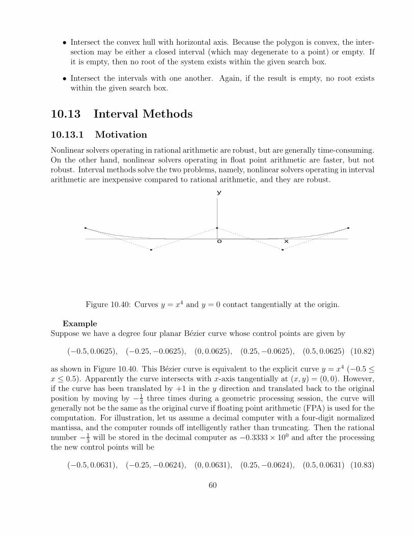
• Intersect the convex hull with horizontal axis. Because the polygon is convex, the inter-section may be either a closed interval (which may degenerate to a point) or empty. Ifit is empty, then no root of the system exists within the given search box.
• Intersect the intervals with one another. Again, if the result is empty, no root existswithin the given search box.
10.13 Interval Methods
10.13.1 Motivation
Nonlinear solvers operating in rational arithmetic are robust, but are generally time-consuming.On the other hand, nonlinear solvers operating in float point arithmetic are faster, but notrobust. Interval methods solve the two problems, namely, nonlinear solvers operating in intervalarithmetic are inexpensive compared to rational arithmetic, and they are robust.
x
y
o
Figure 10.40: Curves y = x4 and y = 0 contact tangentially at the origin.
ExampleSuppose we have a degree four planar Bezier curve whose control points are given by
(−0.5, 0.0625), (−0.25,−0.0625), (0, 0.0625), (0.25,−0.0625), (0.5, 0.0625) (10.82)
as shown in Figure 10.40. This Bezier curve is equivalent to the explicit curve y = x4 (−0.5 ≤x ≤ 0.5). Apparently the curve intersects with x-axis tangentially at (x, y) = (0, 0). However,if the curve has been translated by +1 in the y direction and translated back to the originalposition by moving by − 1
3three times during a geometric processing session, the curve will
generally not be the same as the original curve if floating point arithmetic (FPA) is used for thecomputation. For illustration, let us assume a decimal computer with a four-digit normalizedmantissa, and the computer rounds off intelligently rather than truncating. Then the rationalnumber −1
3will be stored in the decimal computer as −0.3333 × 100 and after the processing
the new control points will be
(−0.5, 0.0631), (−0.25,−0.0624), (0, 0.0631), (0.25,−0.0624), (0.5, 0.0631) (10.83)
60
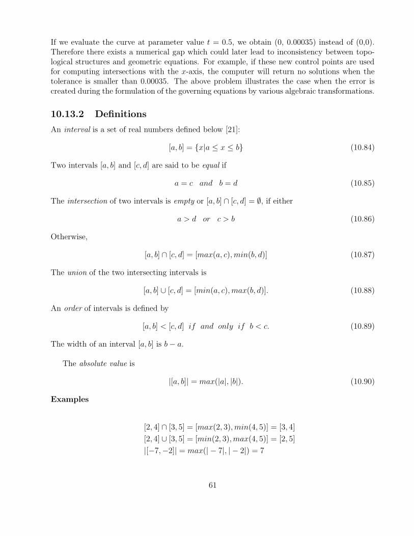
If we evaluate the curve at parameter value t = 0.5, we obtain (0, 0.00035) instead of (0,0).Therefore there exists a numerical gap which could later lead to inconsistency between topo-logical structures and geometric equations. For example, if these new control points are usedfor computing intersections with the x-axis, the computer will return no solutions when thetolerance is smaller than 0.00035. The above problem illustrates the case when the error iscreated during the formulation of the governing equations by various algebraic transformations.
10.13.2 Definitions
An interval is a set of real numbers defined below [21]:
[a, b] = {x|a ≤ x ≤ b} (10.84)
Two intervals [a, b] and [c, d] are said to be equal if
a = c and b = d (10.85)
The intersection of two intervals is empty or [a, b] ∩ [c, d] = ∅, if either
a > d or c > b (10.86)
Otherwise,
[a, b] ∩ [c, d] = [max(a, c), min(b, d)] (10.87)
The union of the two intersecting intervals is
[a, b] ∪ [c, d] = [min(a, c), max(b, d)]. (10.88)
An order of intervals is defined by
[a, b] < [c, d] if and only if b < c. (10.89)
The width of an interval [a, b] is b− a.
The absolute value is
|[a, b]| = max(|a|, |b|). (10.90)
Examples
[2, 4] ∩ [3, 5] = [max(2, 3), min(4, 5)] = [3, 4]
[2, 4] ∪ [3, 5] = [min(2, 3), max(4, 5)] = [2, 5]
|[−7,−2]| = max(| − 7|, | − 2|) = 7
61
10.13.3 Interval Arithmetic
[a, b] ◦ [c, d] = {x ◦ y | x ∈ [a, b] and y ∈ [c, d]}. (10.91)
where ◦ represents an arithmetic operation ◦ ∈ {+,−, ·, /}. Using the end points of the twointervals, we can rewrite equation (10.91) as follows
[a, b] + [c, d] = [a+ c, b+ d]
[a, b] − [c, d] = [a− d, b− c]
[a, b] · [c, d] = [min(ac, ad, bc, bd), max(ac, ad, bc, bd)]
[a, b]/[c, d] = [min(a/c, a/d, b/c, b/d), max(a/c, a/d, b/c, b/d)] (10.92)
provided 0 6∈ [c, d] in the division relation.
Examples
[2, 4] + [3, 5] = [2 + 3, 4 + 5] = [5, 9]
[2, 4] − [3, 5] = [2 − 5, 4 − 3] = [−3, 1]
[2, 4] · [3, 5] = [min(2 · 3, 2 · 5, 4 · 3, 4 · 5), max(2 · 3, 2 · 5, 4 · 3, 4 · 5)] = [6, 20]
[2, 4]/[3, 5] = [min(2/3, 2/5, 4/3, 4/5), max(2/3, 2/5, 4/3, 4/5)] = [2/5, 4/3]
10.13.4 Algebraic Properties
Interval arithmetic is commutative and associative.
[a, b] + [c, d] = [c, d] + [a, b]
[a, b] · [c, d] = [c, d] · [a, b][a, b] + ([c, d] + [e, f ]) = ([a, b] + [c, d]) + [e, f ]
[a, b] · ([c, d] · [e, f ]) = ([a, b] · [c, d]) · [e, f ]
But it is not distributive, however, it is subdistributive.
Examples
[1, 2]([1, 2] − [1, 2]) = [1, 2]([−1, 1]) = [−2, 2]
[1, 2][1, 2] − [1, 2][1, 2] = [1, 4] − [1, 4] = [−3, 3]
10.13.5 Rounded Interval Arithmetic and its Implementation
One has to keep in mind that any sequence of operations on a digital computer is essentiallyequivalent to a finite sequence of manipulations on a discrete grid of points. For example, afloating point number in the general form is given by [11]
(±).d1d2 · · ·dp · 2exp,
62

where d1d2 · · ·dp is mantissa with d1 6= 0, and p is the number of significant digits, and expis the integer exponent. If p = 2 and −2 ≤ exp ≤ 3 then a list of positive numbers in thissystem is
.10 ∗ 2−2 =1
8.11 ∗ 2−2 =
3
16
.10 ∗ 2−1 =1
4.11 ∗ 2−1 =
3
8
.10 ∗ 20 =1
4.11 ∗ 20 =
3
4
.10 ∗ 21 = 1 .11 ∗ 21 =3
2.10 ∗ 22 = 2 .11 ∗ 22 = 3
.10 ∗ 23 = 4 .11 ∗ 23 = 6
0 1−8
1−4
3−8
1−2
3−4
3−2
3−16
1 2 3 4 6
Figure 10.41: Nonnegative floating-point numbers on the interval [0,6], adapted from [11]
If floating–point arithmetic is used to evaluate these interval arithmetic equations there isno guarantee that the roundings of the bounds are performed conservatively. 1.
Most commercial processors implement floating–point arithmetic using the representationdefined by ANSI/IEEE Std 754–1985, Standard for Binary Floating–Point Arithmetic [2]. Thisstandard defines the binary representation of the floating–point number X in terms of a signbit s, an integer exponent E, for Emin ≤ E ≤ Emax, and a p–bit significand (or mantissa) B,where:
X = (−1)s2EB (10.93)
The significand B is a sequence of p bits b0b1 · · · bp−1, where bi = 0 or 1, with an impliedbinary point (analogous to a decimal point) between bits b0 and b1. Thus, the value of B iscalculated as:
1This statement is true only for the default IEEE-754 rounding mode of round towards nearest
63

B = b0.b1b2 · · · bp−1 = b020 +
p−1∑
1
bi2−i (10.94)
For double precision arithmetic, the standard defines p = 53, Emin = −1022, and Emax =1023. The number X is represented as a 64–bit quantity with sign bit s, an 11–bit biased ex-ponent e = E+1023, and a 52–bit fractional mantissa m composed of the bit string b1b2 · · · b52.Since the exponent can always be selected such that b0 = 1 (and thus, 1 ≤ B < 2), the valueof b0 is constant and it does not need to be stored in the binary representation.
63 62 · · · 52 51 · · · 0s e m
The integer value of the 11-bit biased exponent e is calculated as:
e = e0e1 · · · e10 =10∑
0
ei210−i (10.95)
ULP (One Unit in the Last Place)
If x and x′ are consecutive positive double-precision numbers, they differ by an amount εcalled ulp. To calculate ulp it is necessary to extract the integer value of the exponent from thebinary representation. Recall that the value of the significand B of a double precision numberX is:
B = 1 + b12−1 + b22
−2 + · · ·+ b522−52 (10.96)
and that the double precision value X = (−1)s2EB. The value of the least significant bit b52is 2−52. Thus, the value of ulp is 2E2−52 = 2E−52.
Rounded interval arithmetic [19, 20] ensures that the computed end points always containthe exact interval as follows:
[a, b] + [c, d] ≡ [a+ c− ε`, b+ d+ εu][a, b] − [c, d] ≡ [a− d− ε`, b− c+ εu][a, b] · [c, d] ≡ [min(a·c, a·d, b·c, b · d) − ε`,max(a·c, a·d, b·c, b·d) + εu][a, b] / [c, d] ≡ [min(a/c, a/d, b/c, b/d) − ε`,max(a/c, a/d, b/c, b/d) + εu]
(10.97)
where ε` and εu are the units–in–last–place and are denoted by ulp` and ulpu. When per-forming standard operations for interval numbers using RIA, the lower bound is extended toinclude its previous consecutive floating–point number, which is smaller than the lower boundby ulp`. Similarly, the upper bound is extended by ulpu to include its next consecutive num-ber. Thus, the width of the result is enlarged by ulp` + ulpu and the result will be reliable insubsequent operations.
Example
64

main(){
double a = 1.5;
Interval b = 1.5;
double dresult = pow(a, 20.);
Interval iresult = pow(b, 20.);}
dresult 3325.2567300796509
iresult [3325.2567300796404,3325.2567300796613]
10.14 Interval Projected Polyhedron Algorithm
We extend the de Casteljau subdivision method to operate in rounded interval arithmetic inorder to find all the roots of a polynomial system robustly. We illustrate the concept for asingle polynomial equation.
(x - 0.1)(x - 0.6)(x - 0.7) = 0
65

Floating Point Arithmetic
Iter Bounding Box (FPA) Message1 [0,1]2 [0.0763636363636364, 0.856]3 [0.098187732239346, 0.770083868323999]4 [0.0999880766853688, 0.72387404781026] Binary Sub.5 [0.402239977003124, 0.704479954527487]6 [0.550441290533288, 0.700214508664293]7 [0.591018492648952, 0.700000534482207]8 [0.599458794784619, 0.700000000003332] Binary Sub.9 [0.649998841568898, 0.699999999999999] No Root10 [0.599997683137796, 0.649998841568898] Root Found11 [0.099999999478761, 0.402239977003124] Root Found
t
f(t)
������������������������������������������������������������������������������������������������������������������������������������������������������������������������������������������
[P1]
[P2][P0]
t=tAL
t=tBU
Figure 10.42: Interval Projected Polyhedron Method
Rounded Interval Arithmetic
Iter Bounding Box (RIA) Message1 [0, 1]2 [0.076363636363635, 0.856000000000001]3 [0.0981877322393447, 0.770083868324001]4 [0.0999880766853675, 0.723874047810262] Binary Sub.5 [0.402239977003124, 0.704479954527489]6 [0.550441290533286, 0.700214508664294]7 [0.591018492648947, 0.700000534482208]8 [0.599458794784611, 0.700000000003333] Binary Sub.9 [0.649998841568894, 0.7] Root Found10 [0.599997683137788, 0.649998841568895] Root Found11 [0.0999999994787598, 0.402239977003124] Root Found
Most applications mentioned above result in n nonlinear polynomial equations with nunknowns, referred to as balanced systems. However, there exist some problems such as
66

tangential and overlapping intersection or implicit curve/surface rendering consisting of nnonlinear polynomial equations with m unknowns, where n could be larger or smaller than m.When n > m the system is called overconstrained and when n < m it is called underconstrained.Here is an algorithm (the interval n-dimensional Projected-Polyhedron algorithm) such thatit can effectively handle overconstrained problems [15].
Suppose we solve a system of nonlinear interval polynomial equations [f ] = ([f1], [f2], . . . , [fn]) =0 over the box S ∈ Rm (n > m, n = m, n < m) where S is defined by
S = [a1, b1] × [a2, b2] × . . .× [am, bm]. (10.98)
and each [fi] is an interval polynomial in m variables. That is, we wish to find all u ∈ S suchthat
[f1](u) = [f2](u) = . . . = [fn](u) = 0. (10.99)
By making the affine parameter transformation [13] ui = ai + xi(bi − ai) for i = 1, · · ·m, wesimplify the problem to the problem of determining all x ∈ [0, 1]m such that
[f1](x) = [f2](x) = . . . = [fn](x) = 0. (10.100)
Now furthermore suppose that each of the [fk] is polynomial in the independent parameters
x1, x2, . . . , xm. Let d(k)i denote the degree of [fk] in the variable xi; then [fk] can be written in
the multivariate Bernstein basis:
[fk](x) =d(k)1∑
i1=0
d(k)2∑
i2=0
. . .d(k)m∑
im=0
[w(k)i1i2...im ]B
i1,d(k)1
(x1)Bi2,d(k)2
(x2) . . .Bin,d(k)m
(xm). (10.101)
where Bi,m is the ith Bernstein polynomial. The notation in (10.101) may be simplified by
letting I = (i1, i2, . . . im), D(k) = (d(k)1 ,d
(k)2 ,. . .,d(k)
m ) and writing (10.101) in the equivalent form[27]
[fk](x) =D(k)∑
I
[w(k)I ]BI,D(k)(x). (10.102)
Here we have merely rewritten the product of Bernstein polynomials as a single Bernsteinmultinomial BI,D(k)(x). Bernstein polynomials have a useful identity called linear precisionproperty [13], in other words, the monomial t can be expressed as the weighted sum of Bernsteinpolynomials with coefficients evenly spaced in the interval [0, 1]. Using this property, we canrewrite equations (10.102) as follows:
[Fk](x) =D(k)∑
I
[v(k)I ]BI,D(k)(x) (10.103)
where
[v(k)I ] = ([
i1
d(k)1
], [i2
d(k)2
], . . . , [im
d(k)m
], [w(k)I ]). (10.104)
These [v(k)I ] are called the interval control points of [Fk]. Now the algebraic problem of finding
roots of systems of polynomials has been transformed to the geometric problem involving the
67

intersection of the hypersurfaces. Because the problem is now phrased geometrically, we canuse the convex hull property of the multivariate Bernstein basis to bound the set of roots. Wecan structure a root-finding algorithm as follows:
1. Start with an initial box of search.
2. Scale the box and, as we did in converting between equations (10.99) and (10.100),perform an appropriate affine parameter transformation to the functions fk, so that thebox becomes [0, 1]m. However, keep track of the scaling relationship between this boxand the initial box of search. This transformation can be performed with multivariateDe Casteljau subdivision.
3. Using the convex hull property, find a sub-box of [0, 1]m which contains all the roots.The essential idea behind the box generation scheme in this algorithm is to transforma complicated m + 1-dimensional problem into a series of m two-dimensional problems.Suppose Rm+1 can be coordinatized with the x1, x2, . . . , xm+1 axes; we can then employthese steps:
(a) Project the [v(k)I ] of all of the [Fk] into m different coordinate planes; specifically,
the (x1, xm+1)-plane, the (x2, xm+1)-plane, and so on, up to the (xm, xm+1) plane.
(b) In each one of these planes,
i. Construct n two-dimensional convex hulls. The first is the convex hull of theprojected control points of [F1], the second is from [F2] and so on.
ii. Intersect each convex hull with the horizontal axis (that is, xm+1 = 0). Becausethe polygon is convex, the intersection may be either a closed interval (whichmay degenerate to a point) or empty. If it is empty, then no root of the systemexists within the given search box.
iii. Intersect the intervals with one another. Again, if the result is empty, no rootexists within the given search box.
(c) Construct an m-dimensional box by taking the Cartesian product of each one ofthese intervals in order. In other words, the x1 side of the box is the intervalresulting from the intersection in the (x1, xm+1)-plane, and so forth.
4. Using the scaling relationship between our current box and the initial box of search, seeif the new sub-box represents a sufficiently small box in Rm. If it does not, then go tostep 5. If it does, then check the convex hulls of the hypersurface in the new box. Ifthe convex hulls cross each variable axis, conclude that there is a root or at least anapproximate root in the new box, and put the new box into a root list. Otherwise thenew box is discarded (see Appendix for elaboration of this point).
5. If any dimension of this sub-box are not much smaller than 1 unit in length (i.e., thebox has not decreased much in size along one or more sides), split the box evenly alongeach dimension which is causing trouble. Continue on to the next iteration with severalindependent sub-problems.
68
6. If none of the boxes is left, then the root-finding process is over. Otherwise, go back tostep 2, and perform it once for each new box.
If we assume that each equation 10.99 is degree m in each variable and the system is n-dimensional, then the total asymptotic time per step is of O(n2mn+1). The number of stepsdepends primarily on the accuracy required [27].
The Projected Polyhedron Algorithm achieves quadratic convergence in one dimension,while for higher dimensions, it exhibits at best linear convergence.
10.15 Interval Newton method
Interval Newton methods 2 have been the focus of significant attention in numerical analysis.A thorough review of various types of interval Newton methods is presented in [3]. In thesequel we briefly review the interval Newton method. The interval Newton method solves asystem of nonlinear equations in a numerically verifiable manner.
fi(x1, x2, · · · , xn) = 0, 1 ≤ i ≤ n (10.105)
within boxes
ai ≤ xi ≤ bi, 1 ≤ i ≤ n (10.106)
If we denote the n-vector whose ith component is xi by X and the n-vector whose ith componentis fi by F(X), the interval Newton methods can be described as finding a box Xk that containsall the solutions of the interval linear system
J(Xk)(Xk − Xck) = −F(Xc
k) (10.107)
where the subscript k denotes the kth iteration, J(Xk) is the Jacobian matrix of F over thebox Xk, and Xc
k is some point in Xk. There is a theorem about unique solution in the boxgiven by [16]:
TheoremIf Xk is strictly contained in Xk, then the system of equations in (10.105) has a uniquesolution in Xk, and Newton’s method starting from any point in Xk will converge to thatsolution. Conversely, if Xk ∩ Xk is empty, then there are no solutions of the system in(10.105).
The next iteration Xk+1 is evaluated by
Xk+1 = Xk ∩ Xk (10.108)
According to the mean value theorem, the solutions in the Xk must be in Xk+1. If thecoordinate intervals of Xk+1 are smaller than those of Xk, equations (10.107) and (10.108)
2When we use the term “interval Newton method”, we assume that bisection is included in the processwhen interval reduction is not substantial by the pure interval Newton step.
69

are iterated until the bounding boxes are smaller than a specified tolerance. If the coordinateintervals of Xk+1 are not smaller than those of Xk, then one of these intervals is bisected toform two new boxes. The boxes are pushed into a stack and iteration is continued until thestack becomes empty. The first interval Newton method introduced by Moore [21] involvescomputing the inverse of the interval matrix J(Xk). Hansen [12] introduced the Gaussianelimination procedure to solve the linear equation system in an interval Newton method.Krawczyk [12] introduced a variation of the interval Newton method which avoids the Gaussianelimination of an interval matrix by not attempting to obtain a sharp solution of (10.107). Hecomputes the new box Xk as follows
Xk = K(Xk) = Xck − YkF(Xc
k) + (I − YkJ(Xk))(Xk − Xck) (10.109)
where Yk is a preconditioned matrix of midpoints of the elements of the interval Jocobianmatrix. Hansen and Sengupta [12] introduced a box which is generally smaller than K(Xk).They simply solve the ith equation for the ith variable and replace the others by boundingintervals, which is the non-linear version of the Gauss-Seidel operator for linear systems. Let xc
i
be the ith component of Xck and ki be the ith component of YkF(Xk) and Gij be the entry in
the ith row and jth column of YkJ(Xk) then, the step for the ith row of the Hansen-Senguptaoperator becomes
xi = xi − [Gii]−1[ki +
i−1∑
j=1
Gij(xj − xcj) +
n∑
j=i+1
Gij(xj − xcj)] (10.110)
xi = xi ∩ xi
for i = 1, · · · , n.
70

Bibliography
[1] S. L. Abrams, W. Cho, C.-Y. Hu, T. Maekawa, N. M. Patrikalakis, E. C. Sherbrooke, andX. Ye. Efficient and reliable methods for rounded-interval arithmetic. Computer-AidedDesign, 30(8):657–665, July 1998.
[2] ANSI/IEEE Std 754–1985. IEEE Standard for Binary Floating–Point Arithmetic. IEEE,New York, 1985. Reprinted in ACM SIGPLAN Notices, 22(2):9-25, February 1987.
[3] C. Bliek. Computer Methods for Design Automation. PhD thesis, Massachusetts Instituteof Technology, Cambridge, MA, July 1992.
[4] B. Buchberger. Grobner bases: An algorithmic method in polynomial ideal theory. InN. K. Bose, editor, Multidimensional Systems Theory: Progress, Directions and OpenProblems in Multidimensional Systems, pages 184–232. Dordrecht, Holland: D. ReidelPublishing Company, 1985.
[5] J. F. Canny. Generalized characteristic polynomials. Journal of Symbolic Computation,9:241–250, 1990.
[6] G. Dahlquist and A. Bjorck. Numerical Methods. Prentice-Hall, Inc., Englewood Cliffs,NJ, 1974.
[7] R. T. Farouki and V. T. Rajan. Algorithms for polynomials in Bernstein form. ComputerAided Geometric Design, 5(1):1–26, June 1988.
[8] I. D. Faux and M. J. Pratt. Computational Geometry for Design and Manufacture. EllisHorwood, Chichester, England, 1987.
[9] C. B. Garcia and W. I. Zangwill. Global continuation methods for finding all solutionsto polynomial systems of equations in n variables. In A. V. Fiacco and K. O. Kortanek,editors, Extremal Methods and Systems Analysis, pages 481–497. Springer-Verlag, NewYork, NY, 1980.
[10] A. Geisow. Surface Interrogations. PhD thesis, School of Computing Studies and Accoun-tancy, University of East Anglia, Norwich NR47TJ, U. K., July 1983.
[11] C. F. Gerald and P. O. Wheatley. Applied Numerical Analysis. Addison-Wesley, Reading,MA, 4th edition, 1990.
71

[12] E. Hansen and S. Sengupta. Bounding solutions of systems of equations using intervalanalysis. BIT, 21:201–211, 1981.
[13] J. Hoschek and D. Lasser. Fundamentals of Computer Aided Geometric Design. A.K. Peters, Wellesley, MA, 1993. Translated by L. L. Schumaker.
[14] C. Y. Hu, T. Maekawa, N. M. Patrikalakis, and X. Ye. Robust interval algorithm forsurface intersections. Computer-Aided Design, 29(9):617–627, September 1997.
[15] C. Y. Hu, T. Maekawa, E. C. Sherbrooke, and N. M. Patrikalakis. Robust interval algo-rithm for curve intersections. Computer-Aided Design, 28(6/7):495–506, June/July 1996.
[16] R. B. Kearfott and M. Novoa. INTBIS, a portable interval Newton/bisection package(algorithm 681). ACM Transactions on Mathematical Software, 16(2):152–157, June 1990.
[17] G. A. Kriezis, P. V. Prakash, and N. M. Patrikalakis. Method for intersecting algebraicsurfaces with rational polynomial patches. Computer-Aided Design, 22(10):645–654, De-cember 1990.
[18] J. M. Lane and R. F. Riesenfeld. Bounds on a polynomial. BIT: Nordisk Tidskrift forInformations-Behandling, 21(1):112–117, 1981.
[19] T. Maekawa and N. M. Patrikalakis. Computation of singularities and intersections ofoffsets of planar curves. Computer Aided Geometric Design, 10(5):407–429, October 1993.
[20] T. Maekawa and N. M. Patrikalakis. Interrogation of differential geometry properties fordesign and manufacture. The Visual Computer, 10(4):216–237, March 1994.
[21] R. E. Moore. Interval Analysis. Prentice-Hall, Englewood Cliffs, NJ, 1966.
[22] M. E. Mortenson. Geometric Modeling. John Wiley and Sons, New York, 1985.
[23] T. Nishita, T. W. Sederberg, and M. Kakimoto. Ray tracing trimmed rational surfacepatches. ACM Computer Graphics, 24(4):337–345, August 1990.
[24] N. M. Patrikalakis. Surface-to-surface intersections. IEEE Computer Graphics and Ap-plications, 13(1):89–95, January 1993.
[25] N. M. Patrikalakis and P. V. Prakash. Surface intersections for geometric modeling.Journal of Mechanical Design, Transactions of the ASME, 112(1):100–107, March 1990.
[26] H. Pottmann. General offset surfaces. Neural, Parallel and Scientific Computations,5:55–80, 1997.
[27] E. C. Sherbrooke and N. M. Patrikalakis. Computation of the solutions of nonlinearpolynomial systems. Computer Aided Geometric Design, 10(5):379–405, October 1993.
[28] W. I. Zangwill and C. B. Garcia. Pathways to solutions, fixed points, and equilibria.Prentice-Hall, Englewood Cliffs, NJ, 1981.
72