3/23/2015

1

Chapter 13

By Charles I. Jones

Stabilization

Policy and the

AS/AD

Framework

Media Slides Created By

Dave Brown

Penn State University

13.1 Introduction

• In this chapter, we learn:

– With systematic monetary policy, we can combine

the IS curve and the MP curve to get an aggregate

demand (AD) curve.

– That the Phillips curve can be reinterpreted as an

aggregate supply (AS) curve.

– How the AD and AS curves represent an intuitive

version of the short-run model that describes the

evolution of the economy in a single graph.

– The modern theories that underlie monetary

policy.

• Question for this chapter: If we could

formulate a systematic policy in response

to the various kinds of shocks that can

possibly hit the economy, what would the

policy look like?

13.2 Monetary Policy Rules

and Aggregate Demand

• The short-run model consists of three

basic equations:

• The model implies that high short-run

output leads to an increase in inflation.

• The central bank chooses how to make

this trade-off by choosing the interest rate.

• A monetary policy rule

– A set of instructions that determines the

stance of monetary policy for a given situation

that might occur in the economy.

• The rule we consider is that the stance of monetary policy depends on– Current inflation

– Inflation target

• If inflation is above the target– The real interest rate should be high

• If inflation is below the target– The real interest rate should be low

3/23/2015

2

Governs how

aggressively

monetary policy

responds to

inflation

Inflation

target

Current

inflation

• Simple Monetary Policy Rule

Long run

interest

rate

Real

interest

rate

The AD Curve

• We can substitute the monetary policy

rule into the IS curve.

• The resulting equation is the aggregate

demand (AD) curve.

– Says short-run output is a function of the

rate of inflation

• The AD curve

– Describes how the central bank chooses

short-run output based on the rate of inflation.

– Is fundamentally different than market

demand

• If inflation is above target

– The central bank raises the interest rate to

lower output below potential.

Moving along the AD Curve

• A change in inflation

– A movement along the AD curve

• Changes in

– Alter the slope of the AD curve

3/23/2015

3

Shifts of the AD Curve

• AD curve shifts caused by:

– Changes in the parameter

– Changes in the target rate of inflation

13.3 The Aggregate Supply Curve

• The aggregate supply (AS) curve is

– The price-setting equation used by firms

– The Phillips curve with a new name

• Equation:

Current

inflation

Inflation in

last time

period

Parameters

• The point in the graph where short-run

output equals zero is equal to the inflation

rate in the previous period.

• The AS curve will shift due to

– The inflation rate changing over time

– Change in the inflation shock parameter

13.4 The AS/AD Framework

• Combining the AS and AD curve

– Two equations

– Two unknowns

3/23/2015

4

The Steady State

• In the steady state

– the endogenous variables are constant over time

– no shocks to the economy.

– the inflation rate must be constant and short-run

output is equal to zero.

• Steady state implies:

The AS/AD Graph

• The AS curve slopes upward

– implication of price-setting behavior of

firms embodied in the Phillips curve

• The AD curve slopes downward

– Due to the response of policymakers to

inflation.

• The vertical axis represents inflation

• The horizontal axis represents short-run

output.

13.5 Macroeconomic Events

in the AS/AD Framework

• The AS/AD curves allow us to analyze

the dynamics of inflation and output.

Event #1: An Inflation Shock

• The economy begins in steady state and is

hit with a lasting increase in the price of oil.

• Thus, the parameter

– Is positive for one period

– This inflation shock raises the price level

permanently.

• The AS curve will shift up as a result.

• Stagflation

– The stagnation of economic activity

accompanied by inflation.

3/23/2015

5

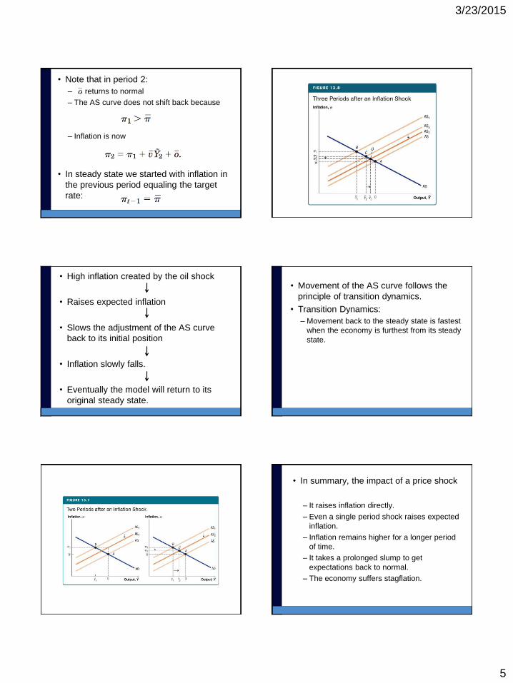
• Note that in period 2:

– returns to normal

– The AS curve does not shift back because

– Inflation is now

• In steady state we started with inflation in

the previous period equaling the target

rate:

• High inflation created by the oil shock

• Raises expected inflation

• Slows the adjustment of the AS curve

back to its initial position

• Inflation slowly falls.

• Eventually the model will return to its

original steady state.

• Movement of the AS curve follows the

principle of transition dynamics.

• Transition Dynamics:

– Movement back to the steady state is fastest

when the economy is furthest from its steady

state.

• In summary, the impact of a price shock

– It raises inflation directly.

– Even a single period shock raises expected

inflation.

– Inflation remains higher for a longer period

of time.

– It takes a prolonged slump to get

expectations back to normal.

– The economy suffers stagflation.

3/23/2015

6

Event 1: Second look:

Suppose the price of oil spikes up and produces

an inflation shock

Short-run output,

Inflation, πt

AS

0

AD

•The math of this is that

the parameter in AS

increases from zero:

•What happens to AS?

• It shifts upward: at

every level of output,

inflation is now higher

•The economy

immediately jumps to a

new temporary

equilibrium at a lower

level of short-run output

and a higher level of inflation

•It turns out that’s only the short-run effect; what

happens next?

AS’

’

’

After the oil shock subsides, inflation

expectations update slowly, and AS will slowly

shift back

Short-run output,

Inflation, πt

0

AD

•We can see from the

Aggregate Supply curve

that inflation stays high

because it was high last

period, even though the

shock subsides and

decreased output pulls it down:

AS’

Now higher

Now negative (lower)

Now zero

•So next, AS shifts

down but not all the way

•Inflation falls a little

while output increases

•Another perspective:

AS’’

’

’

”

”

AS

But we are still not yet back to the steady state, so

the whole process repeats itself, with AS shifting

slowly

Short-run output,

Inflation, πt

0

AD

•The same logic applies:

even with no oil shock

this period, and with

output below potential

pulling inflation down,

inflation will still remain

above its long run level, with gradual steps back

toward steady state

•The steps get smaller

and smaller as the

economy nears steady

state ...

•Sound familiar? This is

like the Solow Model

•An oil shock takes a

while to dissipate!

AS’’

”

”

AS’

AS

Let’s review the time path of output and

inflation after this oil price shock

Short-run output,

Inflation, πt

•Before the oil price

shock hits, inflation is

stable and output is

growing at potential

•When the oil shock hits,

Aggregate Supply shifts

up, immediately raising inflation and lowering

short-run output below

potential

•Since output is below

potential, firms set their

prices lower, reducing

inflation; Aggregate

Supply slowly shifts down, increasing short-

run output back to zero

time, t

time, t

0

Event #2: Disinflation

• Suppose the economy begins in steady

state and policymakers decide to lower

the target rate of inflation.

• The AD curve

– Shifts down

• The new rule calls for

– An increase in interest rates

3/23/2015

7

• The economy must now move to its

new steady state.

• When actual output equals potential

output, the new steady state is at the

new target rate of inflation.

• The change in the rate of inflation

causes the AS curve to shift during the

following period.

• Firms adjust their expectation for

inflation to account for the new lower

inflation rate.

– The AS curve shifts down.

• The inflation rate is still above the

target.

– The central bank keeps actual output

below potential.

– The inflation rate falls further.

• Eventually, the economy will rest in its

new steady state.

• Note that if the classical dichotomy holds

in the short run, the AD and AS curves

would reach the new steady state

immediately.

• If there is sticky inflation, a recession is

needed to adjust expectations down.

3/23/2015

8

Even 2. Second look: The Volcker Disinflation, a

permanent shock to AD

Short-run output,

Inflation, πt

•Suppose the Fed wants

a lower long-run rate of

inflation than is currently

prevailing, and it will use

monetary policy to

achieve it

•The Fed’s monetary policy affects Aggregate

Demand, and not

Aggregate Supply

•The Fed chooses a

lower inflation target,

•Aggregate Demand

shifts inward because

•But the Fed actually

aims for a short-term

intersection above the

final level of inflation!

AS

0

ADAD’

’

’

Just like before, we’re not done - AS also shifts!

Short-run output,

Inflation, πt

•When the Fed starts the

disinflation by lowering

Aggregate Demand,

inflation falls

•A fall in inflation shifts

Aggregate Supply

downward. Why? It’s because firms see the

disinflation and set their

prices accordingly:

•Since inflation has fallen,

πt–1 is lower, so the

intercept term has fallen, causing a downward or

outward shift in the AS

curve

•But AS doesn’t fall all the

way immediately!

AS

0

AD’

’

’

AS’

AD

And just like before, Aggregate Supply slowly

adjusts

Short-run output,

Inflation, πt

•The AS Curve

keeps falling as long

as short-run output is

below zero, because

firms set next

period’s prices that

way:AS’

0

AD’ AD

•Ultimately, the AS

curve reaches the

new steady state at

zero short-run output

(in other words,

output is at potential)

and lower long-run inflation,

AS

The time path of output and inflation after

the Volcker Disinflation, a permanent shift

in AD:

Short-run output,

Inflation, πt

•Before the Fed

switches targets,

inflation is stable but

high and output is

growing at potential

•The Fed chooses a

lower inflation target and raises interest

rates, shifting AD back

and immediately

lowering inflation and

short-run output

•Since output is below

potential, firms set their

prices lower, reducing inflation; Aggregate

Supply slowly shifts

down, increasing short-

run output back to zerotime, t

time, t

0

Event #3: A Positive AD Shock

• Suppose there is a temporary increase in

the aggregate demand parameter

– The AD curve will shift out.

– Prices increase.

3/23/2015

9

• As inflation has increased, firms expect

higher inflation in the future.

• Thus, the AS curve shifts upward over

time.

– The inflation rate associated with zero short-

run output rises.

– The AS curve shifts until the economy has

higher inflation and zero short-run output.

• The aggregate demand shock implies

that booms are matched by recessions.

– The economy benefits from a boom but

inflation rises.

– The way to reduce inflation is by a

recession.

• The costs of inflation:

– The economy would have been better

staying at its original steady state than

going through this cycle.

Event #3: Second look: A temporary positive

shock to Aggregate Demand through exports

Short-run output,

Inflation, πt

AS

0

AD

•Suppose there is a

boom in Europe, and

they demand more U.S.

exports temporarily

•Aggregate Demand

shifts out immediately,

and the economy jumps to the new intersection

•But we’re not done ...

•Aggregate Supply

reacts to increased

inflation by shifting

upward, reducing short-

run output, because

firms adjust their prices:

’

’

AD’

AS’

3/23/2015

10

As before, Aggregate Supply adjusts slowly

because firms are setting their prices

Short-run output,

Inflation, πt

AS

0

AD

•Aggregate Supply shifts

upward as firms set

prices higher and

increase inflation, and

the process stops when

the new AS and the new

AD intersect at

AD’

AS’

•But now: yet another

twist! We’re still not

done. Why? The

Aggregate Demand

shock was only

temporary

•Ultimately, AD will shift back to where it was

initially!

AS’’

AD

The Aggregate Demand shock eventually dies

out, and AD shifts back to where it was

Short-run output,

Inflation, πt

AS

0

•Now, Aggregate

Supply will adjust by

shifting downward,

because short-run

output is negative,

below potential!

•This process returns us slowly to the original

equilibrium! Why?

•The Aggregate

Demand shock, of

Europeans buying

more U.S. exports, is

only temporary

•Things happen in the interim, but in the long

run it “wears off”

AD’

AD

AS’’

AS

AS’’

AD’

The time path of output and inflation after the

temporary Aggregate Demand shock through exports

•Before the export shock

hits, inflation is stable and

output is growing at

potential

•Europeans demand more

U.S. exports, and AD shifts

out, raising output and

inflation immediately

•Aggregate Supply slowly

shifts up, increasing

inflation and lowering short-

run output back to 0

•When the export shock

stops, AD shifts back,

immediately lowering output

and inflation

•Aggregate Supply slowly

shifts down, lowering

inflation and raising output

Short-run output,

Inflation, πt

time, t

time, t

0

Further Thoughts on Aggregate Demand Shocks

• In theory, monetary policy can be used

to insulate an economy from aggregate

demand shocks.

• The monetary policy rule we specified

here responds only to inflation and not

output changes.

13.6 Empirical Evidence

• Question: What are the empirical

predictions of the short-run model when

monetary policy is dictated by an

inflation-based policy rule?

Predicting the Fed Funds Rate

• The Fisher equation

– Monetary policy rule in terms of the nominal

interest rate:

• The Taylor rule suggests picking

parameter values that are functions of 2.

Nominal interest rate

3/23/2015

11

Inflation-Output Loops

• When plotting inflation on the vertical

axis and output on the horizontal axis:

– The economy will follow counterclockwise

loops to shocks in the economy.

– Positive short-run output leads to rising

inflation.

– A rise in inflation leads policymakers to

reduce output.

Case Study: Forecasting and the Business Cycle

• To conduct forecasts, economists study

a large number of variables of leading

economic indicators.

– The fed funds rate

– The term structure for interest rates

– Claims for unemployment insurance

– The number of new houses

• Forecasts have a difficult time predicting

“turning points.”

3/23/2015

12

13.7 Modern Monetary Policy

• The short-run model captures many

features of monetary policy.

• Central banks are now more explicit

about policies and targets.

• Inflation rates in industrialized countries

have been well behaved for the last 25

years.

More Sophisticated Monetary Policy Rules

• Richer monetary policy rules that use

short-run output create results similar to

the simpler model.

– The simple policy rule we used implicitly

weights short-run output.

Rules versus Discretion

• Is there any benefit to creating a

systematic policy?

• The time consistency problem

– Even though an agent supports a particular

policy, once the future comes, they have

incentives to renege on their promises.

• Firms and workers form expectations

about inflation and build them into pricing

decisions.

– Central bankers have incentives to pursue an

expansionary policy.

– Firms and workers anticipate the policy and

build that anticipation into—resulting in no

benefit to output.

• Policymakers need to commit to not

exploit inflation expectations in order to

keep a low rate of inflation.

3/23/2015

13

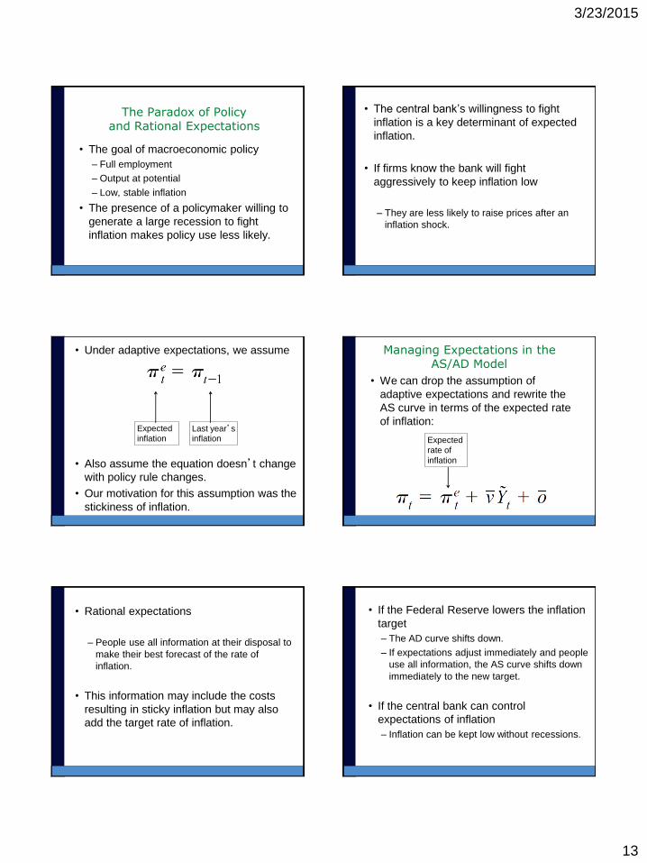
The Paradox of Policy and Rational Expectations

• The goal of macroeconomic policy

– Full employment

– Output at potential

– Low, stable inflation

• The presence of a policymaker willing to

generate a large recession to fight

inflation makes policy use less likely.

• Under adaptive expectations, we assume

• Also assume the equation doesn’t change

with policy rule changes.

• Our motivation for this assumption was the

stickiness of inflation.

Expected

inflationLast year’s inflation

• Rational expectations

– People use all information at their disposal to

make their best forecast of the rate of

inflation.

• This information may include the costs

resulting in sticky inflation but may also

add the target rate of inflation.

• The central bank’s willingness to fight

inflation is a key determinant of expected

inflation.

• If firms know the bank will fight

aggressively to keep inflation low

– They are less likely to raise prices after an

inflation shock.

Managing Expectations in the AS/AD Model

• We can drop the assumption of

adaptive expectations and rewrite the

AS curve in terms of the expected rate

of inflation:

Expected

rate of

inflation

• If the Federal Reserve lowers the inflation

target

– The AD curve shifts down.

– If expectations adjust immediately and people

use all information, the AS curve shifts down

immediately to the new target.

• If the central bank can control

expectations of inflation

– Inflation can be kept low without recessions.

3/23/2015

14

Case Study: Rational Expectations and the Lucas Critique

• The Lucas critique

– It is inappropriate to build a macroeconomic

model based on equations in which

expectations are not consistent with the

statistical properties of the economy.

• Models should incorporate the theory of

rational expectations.

Inflation Targeting

• In many countries, central banks have an

explicit target rate of inflation that they

seek to apply over the medium horizon.

• Explicit inflation targets

– Anchor inflation expectations

– May make it easier for central banks to

stimulate output

• Constrained discretion

– A central bank has the flexibility to respond to

shocks in the short-run.

– The bank is committed to particular rate of

inflation in the long run.

Second look:Rules versus discretion in

monetary policy

• To review: rules are set-in-stone reactions, like the rule we

specified for the Federal Reserve. Discretion refers to the Fed’s

choice whether and when to act

• Why talk about this distinction? Three reasons:

– Mechanically, we need a rule to simplify the short run model from IS-MP-

PC to the Aggregate Supply and Demand model

– Recent economic history suggests that the specific rule we chose is

consistent with the Fed’s actual behavior (this is in section 12.6 in the

text, if you are interested)

– Nobel prizewinning research has revealed why discretionary monetary

policy can actually be bad for the macroeconomy

• How could discretionary policy be bad if policymakers have good

intentions?

Why is discretionary policy dangerous?

• People know how the short-run model works, and they know that

policymakers also know how the short-run model works

• Why is this knowledge dangerous?

• First of all: everyone, including policymakers, likes to have low

inflation and high output at the same time

• What does the IS-MP diagram tell us about the Fed and interest

rates?

• By lowering interest rates, the Fed can stimulate investment and push

output above potential, raising

• What does the Phillips Curve (PC) tell us about output above

potential?

• When , the change in inflation is positive — inflation will rise

• If we know the Fed likes output, we might expect inflation to rise, and

it will, in a self-fulfilling prophecy, because πe is high:

3/23/2015

15

How can the Fed avoid this trap?•Odysseus (a.k.a. the Fed)

really badly wanted to get back

home from the Trojan War

(think of this as having low

inflation)

•But he also really badly

wanted to hear the song of the sirens (think: high output)

•The problem: he knew that if

he and his men listened to the

sirens, sure it would be fun, but

they’d run their ship aground

and die(think: high inflation)

•So he plugged the ears of his

men and tied himself to the mast (think: commit to rule)

Specifying a policy rule is a way of tying

yourself to the mast, so you can’t be tempted

• The rule does not have to ignore output, like our original rule

did, but it does have to convince the public that you will fight

inflation.

• The more convincing you are in promising to fight inflation —

the more tightly you tie yourself to the mast, promising not to

raise short-run output even though you really, really badly

want to ...

• ... the more adaptive Aggregate Supply will be, and the

shorter recessions will last

• Why? If your commitment to a particular inflation target is

credible, then inflation expectations will be equal to that target,

and not necessarily equal to recent inflation:

• How does this look in the AS/AD graph?

Suppose the Fed has garnered credibility and

announces a lower inflation target that people believe

Short-run output,

Inflation, πt

•As in Example #2, the

Fed chooses a new

target

•Aggregate demand will

fall because the Fed

adopts this new target,

since AD is

•But if the Fed announces this change

and has built up its

credibility so that firms

believe it, AS

will simultaneously jump

down as firms price in

exactly

•The result? Less

inflation with no recession!

AS

0

ADAD’

AS’

AS:

Is this for real? Lower inflation

without a recession?• This sounds almost too good to be true, right? We don’t like

inflation, and we don’t like recessions, so doesn’t this kind of

policy fit the bill exactly?

• Yes it does, and this reasoning is behind the use of inflation

targeting by central banks in many countries today: UK,

Australia, Brazil, Canada, Mexico, New Zealand, and Sweden

• But this isn’t a free lunch — credibility is required but not free!

• The only way to make firms believe in your inflation target is to

stick to it, which means raising interest rates and causing a

recession when oil price shocks hit, among other things

• The bottom line: we would still have recessions under fully

credible inflation targeting, and we still believe that flexibility —

the occasional use of discretion — is an important tool to keep

in the toolbox

Case Study: Choosing a Good Federal Reserve Chair

• The Romer and Romer study argues

that policymakers’ views about how the

economy works play a crucial role in

making a good chair.

• Knowledge of macroeconomics is

essential to successful Fed chairs.

Conclusion

• A credible, transparent commitment to a

low rate of inflation is one of the key

factors in taming inflation.

– Anchors inflation expectations so that

shocks are deflected quickly

– Stabilizes economy

• The period after the 1980–82 recession

– “The Great Moderation”

– Relative stability of the macroeconomy

3/23/2015

16

Summary

• Monetary policy often follows a

systematic approach that can be

characterized as a monetary policy rule:

• The central bank increases the real

interest rate whenever inflation exceeds

a particular target.

• This rule describes monetary policy in

the U.S. economy over the last few

decades reasonably well.

• Combining a monetary policy rule with the IS curve leads to an aggregate demand (AD) curve

• AD curve

– Describes how the central bank chooses the level of short-run output based on the current rate of inflation

• The aggregate supply (AS) curve, another name for the Phillips curve

– Tells us that the current rate of inflation depends positively on short-run output

• The equation for the AS curve is:

• In the AS/AD framework, we assume expected inflation adjusts slowly, or is sticky.

• We have adaptive expectations, so that

• The AS/AD framework allows us to study shocks to the economy and changes in the inflation target.

• The graph shows how inflation and short-run output evolve over time.

• The economy moves gradually back to its steady state after a shock.

• Modern monetary policy recognizes that

managing inflation expectations is an

important key to stabilizing the economy.

• The theory of rational expectations

– In order to determine future inflation, people

analyze all information that is available to

them.

• Systematic monetary policy, reputation,

and inflation targets are tools that central

banks use to help them manage inflation

expectations.

• By anchoring inflation expectations,

central banks can achieve low inflation

and stable output in the least costly

fashion.

Macroeconomics

This concludes the Lecture

Slide Set for Chapter 13

by

Charles I. Jones

Third Edition

W. W. Norton & CompanyIndependent Publishers Since 1923