1.3 sliding hinge joint
TRANSCRIPT

http://researchspace.auckland.ac.nz
ResearchSpace@Auckland
Copyright Statement The digital copy of this thesis is protected by the Copyright Act 1994 (New Zealand). This thesis may be consulted by you, provided you comply with the provisions of the Act and the following conditions of use:
• Any use you make of these documents or images must be for research or private study purposes only, and you may not make them available to any other person.
• Authors control the copyright of their thesis. You will recognise the author's right to be identified as the author of this thesis, and due acknowledgement will be made to the author where appropriate.
• You will obtain the author's permission before publishing any material from their thesis.
To request permissions please use the Feedback form on our webpage. http://researchspace.auckland.ac.nz/feedback
General copyright and disclaimer In addition to the above conditions, authors give their consent for the digital copy of their work to be used subject to the conditions specified on the Library Thesis Consent Form and Deposit Licence.
Development of the low damage
self-centering Sliding Hinge
Joint
Khoo Hsen Han
A thesis submitted in partial fulfilment of the requirements for the degree of
Doctor of Philosophy
Supervised by Associate Professor Charles Clifton
The University of Auckland Department of Civil and Environmental Engineering
New Zealand
July 2013

i
Abstract
The Sliding Hinge Joint (SHJ) is a low damage beam-column connection that rotates
inelastically with minimal damage through sliding in Asymmetric Friction Connections
(AFCs). The AFC is a type of slotted bolted connection, which is installed in the bottom
web and bottom flange bolt groups. Previous studies showed that under a major
earthquake, the SHJ undergoes permanent losses in elastic strength due to bolt tension
losses. The frames may also be subject to residual drifts. This thesis presents research
undertaken to better understand and improve the SHJ and AFC, and develop a self-
centering version of the SHJ (SCSHJ).
AFC specimens with shims made of three steel grades were tested to determine the
influence of shim hardness on the frictional performance. Abrasion resistant steel, the
hardest material tested with a specified hardness of 370 – 430 HB, performed the best
with the highest friction, least wear and most stable hysteretic behaviour. Abrasion
resistant steel was therefore recommended for use in future construction. Some of the
specimens were tested with Belleville Springs installed under the nut, where it was found
that the springs increased the sliding shear capacity by reducing the loss in bolt tension
that occurs when sliding takes place. Further AFC tests were conducted to establish
recommended sliding shear capacity values for use in design and residual joint strengths
once subjected to sliding. It was established that the AFC has minimal residual joint
strength after an earthquake and the bolts have to be retightened or replaced.
The proposed SCSHJ incorporates ring springs installed below or above the beam
bottom flange to improve self-centering properties. Ring springs are friction damping
springs that exhibit flag-shape hysteretic behaviour. In the SCSHJ, the ring spring will
partially develop moment resistance, store and release energy which improves self-
centering, and reduce elastic strength losses through pre-stressing. The objective is to
improve dynamic self-centering behaviour, taking shake-down of the building into
account. The SCSHJ thus does not reflect flag-shape hysteretic curves typical of other
self-centering systems. The SCSHJ is designed based on the percentage of ring spring

ii
contribution to total flexural capacity (PRS). Prototype 10-storey frames with the SHJ or
SCSHJ at PRS levels up to 50% were designed and studied analytically using a suite of
10 ground motions, showing reduced residual drifts with increasing PRS. Frames with PRS
of 25% or more had residual drifts under construction tolerance limits for all ground
motions scaled to the Design Level Event. The level of PRS investigated was however
insufficient to significantly increase the elastic strength of the post-earthquake joint. The
benefits of the ring springs were limited under the ground motions scaled to the
Maximum Considered Event due to the high drift demands.
Experimental tests of the SHJ and SCSHJ were undertaken on a full-scale subassembly
representing an internal connection. The joints tested ranged from the standard SHJ to
the Ring Spring Joint, where the flexural capacities of the latter were developed only by
ring springs. The joint self-centering hysteretic response improved with increasing PRS.
The hysteretic models used in previous analytical studies of the joints were modified
based on the experimental results. Further analytical studies on the 5 and 10 storey
frames showed the viability of using ring spring at selected joints within the frame to
reduce overall cost.

iii

iv

v

vi
vii
Acknowledgements
I would like to sincerely thank my supervisors Assoc. Professor Charles Clifton and
Assoc. Professor John Butterworth for their support, patience, contribution and
encouragement throughout this research project, and to Assoc. Professor Gregory
MacRae whose constant involvement was extremely helpful. I would also like to thank
Professor George Ferguson and Dr Chris Seal for their time and contribution to this
research.
The experimental testing in this research was financially supported by the New Zealand
Earthquake Commission (EQC) and material donations and discounts from Grayson
Engineering, Ringfeder Gmbh and Composite Floor Decks. Many thanks to Jeffrey Ang,
Daniel Ripley, Mark Byrami, Noel Perinpanayagam and Sujith Padiyara for assistance
during the experimental testing of this project, and to Christopher Mathieson, Steven
Yeung and Hao Zhou who conducted some of the testing in this research.
I would like to extend my deepest gratitude to my parents Khoo Chin Teng and Su Bee
Yan, and my sister Khoo Hsu-Ee for their unwavering support. Thank you for your love,
understanding, patience, encouragement and countless sacrifices over the past 26 years.
Without you, this would not have been possible. Many thanks also to my friends for
support and encouragement, and to my colleagues for friendship and insights over the
past three years. Special mention goes to Chong Yoong Xiong, Lee Jun Bin, Michelle Ho,
Elena Ching, Adane Sibani and Liu Tingting.
This thesis is testimony to the grace and faithfulness of God (Lamentations 3:22-24) and
to Him who gives me strength (Philippians 4:13).
Soli Deo Gloria


ix
Table of contents
Abstract ...................................................................................................................... i
Acknowledgments .................................................................................................. vii
Table of contents ..................................................................................................... ix
List of figures .......................................................................................................... xv
List of tables ............................................................................................................ xx
Notation ................................................................................................................. xxi
1 Introduction ........................................................................................................ 1
1.1 Overview......................................................................................................................... 2
1.2 Literature Review ........................................................................................................... 3
1.2.1 Rigid connections ................................................................................................ 3
1.2.2 Slotted bolted connection (SBC) ....................................................................... 5
1.2.3 Post-tensioned systems ....................................................................................... 7
1.2.4 Shape memory alloy systems ............................................................................ 10
1.3 Sliding Hinge Joint ...................................................................................................... 13
1.3.1 Joint configuration ............................................................................................ 13
1.3.2 Rotational behaviour ........................................................................................ 14
1.3.3 Experimental studies ........................................................................................ 17
1.3.4 Analytical studies ............................................................................................... 19
1.3.5 Bolt model ......................................................................................................... 20
1.3.6 Advantages and limitations .............................................................................. 23
1.3.7 Research limitations prior to this project ...................................................... 24
1.4 Objectives and scope .................................................................................................. 25
1.5 Thesis outline ............................................................................................................... 30
1.6 References .................................................................................................................... 33
2 Behaviour of the top and bottom flange plates in the Sliding Hinge Joint .. 39
2.1 Introduction ................................................................................................................. 40
2.2 Design considerations and behaviour of the bottom and top flange plates ....... 42
2.2.1 Design philosophy ........................................................................................... 42

x
2.2.2 Demand ............................................................................................................... 45
2.3 Weld behaviour ............................................................................................................ 51
2.4 Flange plates ................................................................................................................. 53
2.4.1 Damage model ................................................................................................... 53
2.4.2 Comparison with design provisions ................................................................ 56
2.5 Top flange plate elongation ........................................................................................ 58
2.6 Limitations .................................................................................................................... 60
2.7 Conclusions .................................................................................................................. 60
2.8 References ..................................................................................................................... 61
3 Influence of steel shim hardness on the Sliding Hinge Joint performance ..... 65
3.1 Introduction.................................................................................................................. 66
3.2 Behaviour of the Sliding Hinge Joint ........................................................................ 69
3.3 Test description ............................................................................................................ 73
3.4 Friction and Wear ........................................................................................................ 77
3.5 Test results .................................................................................................................... 82
3.5.1 Mild steel (G300) shims .................................................................................... 83
3.5.2 High strength quenched and tempered (G80) steel shims ........................... 85
3.5.3 Abrasion resistant (G400) steel shims ............................................................. 86
3.5.4 Material wear....................................................................................................... 89
3.5.5 Comparison with bolt model ........................................................................... 91
3.6 Discussion ..................................................................................................................... 92
3.7 Summary and conclusions .......................................................................................... 95
3.8 References ..................................................................................................................... 96
4 Sliding shear capacity and residual strength of the Asymmetric Friction
Connection ...................................................................................................... 101
4.1 Introduction................................................................................................................ 103
4.1.1 Sliding shear capacity (Vss) .............................................................................. 103
4.1.2 Residual joint strength (SR) ............................................................................. 107
4.2 Test description .......................................................................................................... 107
4.2.1 Test setup .......................................................................................................... 107

xi
4.2.2 Loading regime ................................................................................................. 110
4.2.3 Test specimens ................................................................................................. 114
4.3 Results and discussion .............................................................................................. 117
4.3.1 Strain gauge/load cell tests ............................................................................. 117
4.3.2 Bolt model ........................................................................................................ 124
4.3.3 Sliding shear capacity ....................................................................................... 129
4.3.4 Residual joint strength (SR) ............................................................................. 134
4.4 Limitations and recommendations.......................................................................... 137
4.5 Conclusions ................................................................................................................ 138
4.6 References .................................................................................................................. 139
5 Development of the self-centering Sliding Hinge Joint with friction ring
springs .......................................................................................................... 141
5.1 Introduction ............................................................................................................... 142
5.2 Joint behaviour .......................................................................................................... 145
5.2.1 SHJ ..................................................................................................................... 145
5.2.2 Ring springs ...................................................................................................... 147
5.2.3 SCSHJ ................................................................................................................ 149
5.2.4 Residual deformations ..................................................................................... 151
5.3 Building and modelling ............................................................................................. 153
5.3.1 MRF description .............................................................................................. 153
5.3.2 Design objectives ............................................................................................. 154
5.4 Analytical models ....................................................................................................... 157
5.5 Time history analysis ................................................................................................. 158
5.5.1 Ground motions and performance levels .................................................... 158
5.5.2 Response parameters ....................................................................................... 159
5.6 Results and Discussion ............................................................................................. 160
5.6.1 Peak and residual storey drift responses ....................................................... 160
5.6.2 Moment-rotational characteristics ................................................................. 164
5.6.3 Residual joint strength..................................................................................... 166
5.7 Limitations and challenges ....................................................................................... 168
5.8 Summary and conclusions ........................................................................................ 169

xii
5.9 References ................................................................................................................... 170
6 Experimental study of full-scale self-centering Sliding Hinge Joint
connections with friction ring springs ............................................................ 175
6.1 Introduction................................................................................................................ 176
6.2 Joint description ......................................................................................................... 179
6.2.1 Sliding Hinge Joint ........................................................................................... 179
6.2.2 Ring Spring Joint .............................................................................................. 182
6.2.3 Self-centering Sliding Hinge Joint.................................................................. 185
6.3 Subassembly Test Description ................................................................................. 186
6.3.1 Test setup .......................................................................................................... 186
6.3.2 Test details ........................................................................................................ 189
6.3.3 Test procedure .................................................................................................. 192
6.4 Results and discussion ............................................................................................... 193
6.4.1 Sliding Hinge Joint behaviour ........................................................................ 195
6.4.2 Ring Spring Joint behaviour ........................................................................... 196
6.4.3 Self-centering Sliding Hinge Joint behaviour ............................................... 199
6.4.4 Loading rate effects ......................................................................................... 200
6.4.5 Near fault type action performance............................................................... 200
6.4.6 Secondary element effects .............................................................................. 201
6.4.7 Slab damage ...................................................................................................... 203
6.5 SCSHJ model .............................................................................................................. 204
6.6 Summary and conclusions ........................................................................................ 206
6.7 References ................................................................................................................... 207
7 Analytical studies of the SHJ and SCSHJ ....................................................... 211
7.1 Introduction................................................................................................................ 211
7.2 Joint modelling ........................................................................................................... 214
7.2.1 Rotational springs ............................................................................................ 214
7.2.2 Original SHJ model (IHYST_42_2005) ....................................................... 214
7.2.3 Comparison of IHYST_42 _2005 with experimental results .................... 219
7.2.4 Modifications to SHJ model (IHYST 42) ..................................................... 223

xiii
7.2.5 Joint modelling discussion .............................................................................. 231
7.3 Time-history analysis ................................................................................................. 233
7.3.1 Performance objectives ................................................................................... 233
7.3.2 Frame description ............................................................................................ 234
7.3.3 Joint design and modelling ............................................................................. 235
7.3.4 Ground motions .............................................................................................. 241
7.3.5 Results ............................................................................................................... 242
7.3.6 Time-history analysis discussion .................................................................... 249
7.4 Limitations .................................................................................................................. 253
7.5 Recommendations ..................................................................................................... 255
7.6 Conclusions ................................................................................................................ 256
7.7 References .................................................................................................................. 257
8 Summary and conclusions .............................................................................. 251
8.1 Summary ..................................................................................................................... 252
8.1.1 Bottom and top flange plate behaviour ........................................................ 252
8.1.2 Dynamic behaviour of steel shims of different hardness .......................... 252
8.1.3 Sliding shear capacity and residual joint strength ........................................ 253
8.1.4 Self-centering Sliding Hinge Joint ................................................................. 254
8.1.5 Effects of ring spring component in the SCSHJ ......................................... 255
8.1.6 Experimental behaviour of full-scale SHJ and SCSHJ ............................... 256
8.1.7 Time-history analysis of SCSHJ frames ........................................................ 257
8.2 Conclusions ................................................................................................................ 258
8.3 Original contributions of research .......................................................................... 259
8.4 Future Work ............................................................................................................... 260
8.4.1 Asymmetric Friction Connection .................................................................. 260
8.4.2 Sliding Hinge Joint and Self-Centering Sliding Hinge Joint ...................... 260
Appendix A: Asymmetric Friction Connetion details ........................................... 275
A.1 Detailed dimensions of specimens .......................................................................... 275
A.2 Sliding shear capacity design tables ......................................................................... 278
A.3 References .................................................................................................................. 280

xiv
Appendix B: Full scale subassembly test details .................................................. 281
B.1 Test setup figures ....................................................................................................... 282
B.2 Ring spring cartridge figures .................................................................................... 286
B.3 Ring spring cartridge force-displacement behaviour ............................................ 289
B.4 Instrumentation ......................................................................................................... 290
B.5 Test figures ................................................................................................................. 292
B.6 References ................................................................................................................... 294
Appendix C: Supplementary information for time-history analyses .................... 295
C.1 References ................................................................................................................... 308

xv
1 List of figures
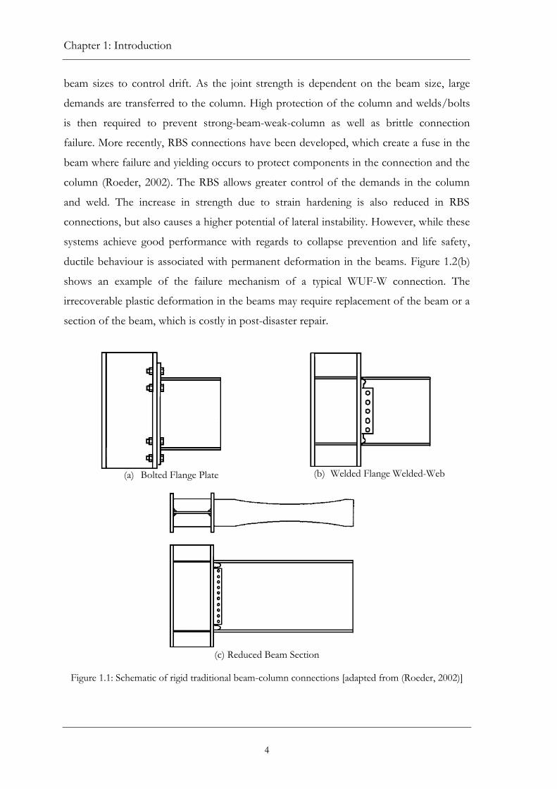
Figure 1.1: Schematic of rigid traditional beam-column connections [adapted from (Roeder, 2002)] ................................................................................................. 4
Figure 1.2: Welded Flange Welded Web (a) moment rotational curve (Roeder, 2002) and (b) beam hinging mechanism (Ricles et al., 2002). .............................. 5
Figure 1.3: Details of slotted bolted connection (Grigorian et al., 1993) .............................. 6
Figure 1.4: Rotational slotted bolted connections (Yang and Popov 1995) ......................... 6
Figure 1.5: Ring spring joint (Clifton 2005) ............................................................................... 8
Figure 1.6: Dual directional ring spring seismic damper (Filiatrault et al., 2000) ................. 8
Figure 1.7: PT connection with friction devices (Iyama et al., 2009) ..................................... 9
Figure 1.8: Behaviour of PT connection with bottom flange friction device (Kim and Christopoulos, 2008) ............................................................................. 10
Figure 1.9: Stress–strain temperature diagram showing deformation and shape memory behaviour of NiTi shape memory alloy (Desroches et al., 2004) ................................................................................................................ 10
Figure 1.10: Connections for MRFs using SMA (a) bolts (Ma et al., 2008), and (b) tendons (Ocel et al., 2004) ................................................................................ 12
Figure 1.11: Sliding Hinge Joint layout (not to scale) (MacRae et al., 2010) ....................... 14
Figure 1.12: Positive and negative rotation of the SHJ .......................................................... 14
Figure 1.13: (a) AFC in the bottom flange plate and (b) AFC idealised force-displacement behaviour .......................................................................................... 16
Figure 1.14: Experimental moment-rotational behaviour of Test 3 from Clifton (2005) ........................................................................................................... 17
Figure 1.15: AFC idealised bolt deformation, external forces and bending moment distribution ................................................................................................ 21
Figure 2.1: Sliding Hinge Joint layout ....................................................................................... 40
Figure 2.2: Joint rotation (web plate not shown for clarity) .................................................. 43
Figure 2.3: Longitudinal strain distribution under positive and negative moment for (a) bottom flange plate and (b) top flange plate ............................ 47
Figure 2.4: Strain relationship under 30 mrad design rotation for (a) longitudinal strain and r = feff/tp, (b) shear strain and feff and (c) longitudinal and equivalent strain and r = feff/tp ................................................... 48
Figure 2.5: Shear demands (a) slip between beam and web plate under negative rotation and (b) shear deformation in flange plates ............................ 49
Figure 2.6: HERA small scale test specimens (Seal et al., 2009) ........................................... 52
Figure 2.7: Small scale test rig (Khoo et al., 2012a) [Chapter 3] ........................................... 52
Figure 2.8: Relationship between number of cycles to failure Nf and (a) strain, and (b) r = feff/tp for longitudinal strain and equivalent strain where tp = 10 and 32 mm ................................................................................................... 55
Figure 2.9: Top flange plate core elastic area under negative rotation................................. 59
Figure 3.1: Sliding Hinge Joint layout [MacRae et al. (2012)] ................................................ 69
Figure 3.2: Beam rotation and idealised moment-rotation curve [MacRae et al.(2010)] .................................................................................................................... 70

xvi
Figure 3.3: Idealised deformation, external force and moment distribution on bolt [modified from MacRae et al. (2010)] ........................................................... 72
Figure 3.4: Test setup .................................................................................................................. 73
Figure 3.5: Sliding bolt component ........................................................................................... 75
Figure 3.6: Brass against G300 sliding characteristics [Clifton (2005)] ................................ 77
Figure 3.7: Real and apparent contact areas [modified from Rabinowicz (1995)] ........................................................................................................................ 79
Figure 3.8: Adhesive wear [modified from Rabinowicz (1995)] ........................................... 80
Figure 3.9: Abrasive wear [modified from Stachowiak et al. (2005)] ................................... 80
Figure 3.10: Hysteresis curves for G300, G80 and G400 shims, with and without Belleville Springs. ....................................................................................... 87
Figure 3.11: Cumulative travel versus force for G300, G80 and G400 shims, with and without Belleville Springs. ...................................................................... 88
Figure 3.12: Surface of cleats. Left to right: G300, G80 and G400...................................... 90
Figure 3.13: Surface of shims. Left to right: G300, G80 and G400. .................................... 91
Figure 3.14: Surface of beam flange plate. Left to right: G300, G80 and G400. ............... 91
Figure 4.1: Finite element analysis model of the AFC (Clifton 2005) ................................ 104
Figure 4.2: Bolt tension vs relative slip between beam flange and cleat (Clifton 2005)......................................................................................................................... 104
Figure 4.3: AFC idealised bolt deformation, external forces and bending moment distribution .............................................................................................. 105
Figure 4.4: Test rig ..................................................................................................................... 108
Figure 4.5: Specimen installed on top of rig with displacement gauges............................. 109
Figure 4.6: AFC specimen installed with bolt rows indicated. Left to right: top side and bottom (beam flange plate) view .......................................................... 109
Figure 4.7: Instrumentation of AFC component tests ......................................................... 110
Figure 4.8: Loading A consisting of Dy1, QE, Dy2, QE and Dy2....................................... 111
Figure 4.9: Comparison between strain gauge and load cell readings in M20.16.T4 (bolt in Row 1) and M20.16.T5 (bolt in Row 2) ............................ 118
Figure 4.10: Hysteretic behaviour of strain gauged tests (M20.16.T3, M20.16.T4 and M20.16.T5) .................................................................................. 119
Figure 4.11: Bolt tension vs AFC displacement for M20.16.T3 (strain gauge reading) .................................................................................................................... 121
Figure 4.12: Bolt tension vs AFC displacement (slip) ........................................................... 122
Figure 4.13: Prying of the AFC under positive (tension) and negative (compression) loading ........................................................................................... 124
Figure 4.14: Vss/2N vs time for strain gauged tests (M20.16.T3, M20.16.T4 and M20.16.T5)....................................................................................................... 126
Figure 4.15: Computed and measured AFC test strengths without Belleville Springs ..................................................................................................................... 131
Figure 4.16: Test results from first round of component testing ....................................... 132
Figure 4.17: Computed and measured AFC test strengths with Belleville Springs ..................................................................................................................... 133
Figure 4.18: AFC without Belleville springs comparison of initial and residual joint strength (%) in compression and tension .................................................. 136
Figure 4.19: AFC with Belleville springs comparison of initial and residual joint strength (%) in compression and tension .................................................. 136
Figure 5.1: SHJ layout ............................................................................................................... 144

xvii
Figure 5.2: (a) Idealised moment-rotational behaviour (MacRae et al., 2010) and (b) components of the bottom flange AFC ................................................ 146
Figure 5.3: Ring spring subassembly (Ringfeder Gmbh, 2008) .......................................... 147
Figure 5.4: (a) SCSHJ layout and (b) ring spring assembly .................................................. 149
Figure 5.5: Idealised moment rotational behaviour .............................................................. 151
Figure 5.6: Shake-down effect in the SHJ [modified from Clifton (2005)] ....................... 152
Figure 5.7: (a) Building plan and (b) MRF layout and member sizes ................................. 153
Figure 5.8: Connection modelling ........................................................................................... 158
Figure 5.9: Relationship between PRS and drift distribution:(a) DLE peak drifts, δp, and (b) MCE peak drifts, δp, (c) DLE residual drifts, δr, and (d) MCE residual drifts, δr. ............................................................................ 161
Figure 5.10: Mean storey drift distribution under the (a) DLE and (b) MCE .................. 162
Figure 5.11: Moment-rotational response in Frames 1 and 4 ............................................. 165
Figure 5.12: Response of storey 9 joint under second El Centro 1979 SLE event ......................................................................................................................... 167
Figure 5.13: Roof displacement under El Centro 1979 compound ground motion ..................................................................................................................... 167
Figure 6.1: Joint layout (a) SHJ and (b) SCSHJ ..................................................................... 177
Figure 6.2: Bottom flange AFC layout and idealised force-displacement characteristics.......................................................................................................... 181
Figure 6.3: SHJ moment-rotational behaviour spine curve ................................................. 182
Figure 6.4: (a) Ring spring cartridge and (b) idealised force-displacement behaviour................................................................................................................. 183
Figure 6.5: Theoretical ring spring moment-rotational behaviour ..................................... 184
Figure 6.6: Idealised moment rotational behaviour (i) SHJ, (ii) RSJ and (iii) SCSHJ (including strength degradation and load history dependence) ............................................................................................................ 186
Figure 6.7: Test setup ................................................................................................................ 187
Figure 6.9: Ring spring cartridge ............................................................................................. 191
Figure 6.10: Assembled SCSHJ ............................................................................................... 191
Figure 6.11: Load regimes: (a) SAC, (b) SAC_Dy, (c) EQ and (d) NF ............................. 193
Figure 6.12: Cyclic response of Test 1 (SHJ) and Test 9 (RSJ): (a) Test 1 load-drift, (b) Test 9 load-drift, (c) Test 1 joint moment-rotation and (d) Test 9 joint moment-rotation ............................................................................... 197
Figure 6.13: Moment-rotational behaviour ............................................................................ 202
Figure 6.14: Slab damage .......................................................................................................... 204
Figure 6.15: Comparison between model and experimental results ................................... 206
Figure 7.1: IHYST_42_2005 spine curve and quadrants ..................................................... 215
Figure 7.2: Calculation of constant mv .................................................................................... 218
Figure 7.3: Rotation vs mv relationship for SHJ without BeS in quadrants PL and NU .................................................................................................................... 219
Figure 7.4: Comparison between Test 1 and IHYST_42_2005 model under the SAC regime (only response from cycles in green) ...................................... 220
Figure 7.5: Comparison between Test 1 and IHYST_42_2005 model under winding down cycles (response from cycles in green) ...................................... 222
Figure 7.6: Proposed changes to IHYST 42 model (changes shown in red) .................... 224
Figure 7.7: Modifications to calculation of C2 in the model ................................................ 225
Figure 7.8: Comparison of proposed model with experimental results ............................. 226

xviii
Figure 7.9: Comparison of IHYST_42_2005 and IHYST_42_2012 models with Test 1 results for cycles up to approximately 15 mrad rotations (only green section of load history) .................................................... 228
Figure 7.10: Comparison of IHYST_42_2012 model with Test 1 results (SAC and winding down response) ................................................................................ 228
Figure 7.11: Comparison between revised model and experimental results for Test 6 under Tabas (only green section of load history) .................................. 230
Figure 7.12: Comparison between revised model and experimental results for Test 6 under El Centro 1979 (only green section of load history) .................. 230
Figure 7.13: Floor plan of 5-storey prototype building [modified from (Clifton 2005)] ........................................................................................................ 235
Figure 7.14: SCSHJ with two ring springs above bottom flange plate ............................. 236
Figure 7.15: SHJ, SCSHJ and RSJ distribution in Frames 7, B and C. ............................... 238
Figure 7.16: Frame peak drift distribution: (a) 10-storey DLE, (b) 5-storey DLE, (c) 10-storey MCE and (d) 5-storey MCE ............................................... 244
Figure 7.17: Frame residual drift distribution: (a) 10-storey DLE, (b) 5-storey DLE, (c) 10-storey MCE and (d) 5-storey MCE. .............................................. 245
Figure 7.18: Mean storey drift distribution (a) 10-storey DLE, (b) 10-storey MCE, (c) 5-storey DLE and (d) 10-storey MCE ............................................... 246
Figure 7.19: 5-storey frame residual drift distribution under the MCE level for (a) El Centro 1979 and (b) other records excluding El Centro 1979.............. 248
Figure 7.20: Moment-rotational response of the internal column on the 3rd storey of the 5-storey frames under the TCU ground motion scaled to the DLE event........................................................................................ 251
Figure 7.21: Moment-rotational response of the external column on the 3rd storey of the 5-storey frames under the TCU ground motion scaled to the DLE event........................................................................................ 251
Figure 7.22: Moment-rotational response of an internal column on the 3rd storey of the 5-storey frames under the Caleta ground motion scaled to the MCE event ....................................................................................... 252
Figure 7.23: Moment-rotational response of the internal column on the 3rd storey of the 5-storey frames under the Caleta ground motion scaled to the MCE event ....................................................................................... 252
Figure A-1: Bottom flange plate (cleat) .................................................................................. 276
Figure A-2: Shim, cap plate and beam flange plate ............................................................... 277
Figure B-3: South side SHJ....................................................................................................... 282
Figure B-4 Test setup prior to installation of floor slab....................................................... 283
Figure B-5: Partway through installation of steel deck ......................................................... 283
Figure B-6: Test setup with deck and reinforcing mesh ...................................................... 284
Figure B-7: Concrete slab at the column slab base prior to testing .................................... 284
Figure B-8: Test setup ............................................................................................................... 285
Figure B-9: Unassembled Type 08000 ring spring cartridge consisting of the cage and cover plate ............................................................................................... 286
Figure B-10: Type 08000 ring spring cartridge with uncompressed ring springs ...................................................................................................................... 287
Figure B-11: Assembled Type 08000 ring spring cartridge.................................................. 287
Figure B-12: Fully installed SCSHJ with ring spring cartridge bolted to bottom flange of beam .......................................................................................... 287

xix
Figure B-13: Nut tightened at the end of the ring spring cartridge .................................... 288
Figure B-14: Nuts tightened on both sides of the column flange ...................................... 288
Figure B-15: Force displacement behaviour of the Type 08000 ring spring cartridges ................................................................................................................. 289
Figure B-16: Force displacement behaviour of the Type 12400 ring spring cartridges ................................................................................................................. 289
Figure B-17: Instrumentation of the connections ................................................................ 290
Figure B-18: Instrumentation of the test setup ..................................................................... 290
Figure B-19: Instrumented panel zone ................................................................................... 291
Figure B-20: Deformation of assembly at 3% drift .............................................................. 292
Figure B-21: Ring spring deformation .................................................................................... 293
Figure B-22: Force-drift behaviour of Test 8 ........................................................................ 293
Figure B-23: Comparison of the joint moment-rotational behaviour in Test 8 with the modified model ....................................................................................... 293
Figure C-24: Response spectra of ground motions for DLE (10-storey frame on rock, T1 = 1.76 secs, Z = 0.4)....................................................................... 297
Figure C-25: Response spectra of ground motions for DLE (5-storey on deep soil, T1 = 1.41 secs, Z = 0.4) .............................................................................. 297

xx
List of tables
Table 1.1: Timeline of work and outputs from research programme .................................. 27
Table 3.1: Summary of material hardness tests ....................................................................... 75
Table 3.2: Test results ................................................................................................................. 83
Table 4.1: Details of AFC test specimen ................................................................................ 115
Table 4.2: Summary of results from coefficient of friction tests ........................................ 126
Table 4.3: Average test results for AFCs without Belleville Springs .................................. 129
Table 4.4: Average test results for AFCs with Belleville Springs ........................................ 129
Table 4.5: Average residual joint strength results for AFCs without Belleville Springs ..................................................................................................................... 135
Table 4.6: Average residual joint strength results for AFCs with Belleville Springs ..................................................................................................................... 135
Table 5.1: Joint details ............................................................................................................... 156
Table 5.2: Summary of individual ground motions .............................................................. 158
Table 5.3: Summary of compound ground motions ............................................................ 159
Table 5.4: Summary of frame maximum and residual drifts under DLE and MCE ground motions ........................................................................................... 160
Table 6.1: Test details – joint design, loading regime and order of tests. .......................... 191
Table 6.2: Details of ring spring cartridges ............................................................................ 191
Table 6.3: Test results ............................................................................................................... 194
Table 7.1: Summary of constants in the SHJ_IHYST_42 model ....................................... 217
Table 7.2: Joint details for Frames 1, 6 and 7, and Frames A, B and C. ............................ 240
Table 7.3: Summary of ground motions for 5-storey frame ................................................ 241
Table 7.4: Summary of results under DLE and MCE ground motions for Frames 1, 6, 7, A, B and C – mean δp, δr, Δp, and number of ground motions exceeding damage thresholds .................................................. 242
Table A-1: Bottom flange plate (cleat), shim, cap plate and bottom flange plate dimensions in millimetres for each AFC size combination of bolt and cleat thickness (tcl) ................................................................................... 276
Table A-2: Sliding shear capacity from (Clifton, 2007) ........................................................ 278
Table A-3: Revised sliding shear capacities from Chapter 4 ............................................... 279
Table B-1: Displacement gauge description .......................................................................... 291
Table C-1: RUAUMOKO input parameters for comparison with full scale joint test results ....................................................................................................... 296
Table C-2: Input control parameters for time-history analysis in RUAUMOKO. ....................................................................................................... 298
Table C-3: Example of RUAUMOKO input file (Frame B) .............................................. 299
Table C-4: Input element property descriptions for time-history analysis in RUAUMOKO. ....................................................................................................... 307

xxi
Notation
Roman
aep Edge distance from beam end to top flange bolt group
A Plate cross-sectional area
Aa Apparent frictional contact area
Ar Real frictional contact area
d Nominal bolt diameter
db Beam depth
dc Column depth
dtravel Total travel distance in the AFC
eRS Distance between ring spring and point of joint rotation
ewb Distance between web bottom bolt group and point of joint rotation
E Elastic modulus
fc’ Concrete compressive strength
F Ring spring capacity
feff Effective length of curvature in the flange plates during inelastic SHJ rotation
fSHJ Clearance between the column flange and beam end
fuf Ultimate tensile strength
Fp Ring spring precompression force
H Column height in full-scale SHJ tests
Hf Final actuator force in full-scale SHJ tests
kin Joint rotational inelastic stiffness
ko Joint rotational elastic stiffness
kr Ring spring contribution to inelastic rotational stiffness in RSJ and SCSHJ
ks Ring spring stiffness
l Bolt lever arm length (distance between points of bearing)

xxii
le Length of elastic core area in the top flange plate
ln Lever arm (l) normalised by bolt diameter
Lp Length of compressed ring spring in RSJ and SCSHJ
mv Joint softening factor
M Moment
M25 Moment resistance at 25 mrad rotation
Md Dependable moment, defined as MSHJ,0 + MRS,y
Mdes Large-scale test joint design capacity
MDLE* Moment demand (design level earthquake spectrum)
Mo Moment at zero displacement in final cycle of loading
MPT Post-tensioned force contribution to joint moment
Mrfn Bolt moment capacity considering axial force interaction
MRSJ RSJ design moment (ring spring contribution to joint moment in SCSHJ)
MSHJ Sliding Hinge Joint design moment (AFC contribution to moment in SCSHJ)
MSCSHJ Self-centering Sliding Hinge Joint design moment
MSLE* Moment demand (serviceability level earthquake spectrum)
My Yield moment
ne Number of ring spring elements
nbfb Number of bolts in the bottom flange plate
nwbb Number of bolts in the bottom web AFC bolt group
np2.5 Number of ground motions exceeding peak drift limit of 2.5%
nr0.1 Number of ground motions exceeding residual drift limit of 0.1%
nr0.1 Number of ground motions exceeding residual drift limit of 0.2%
N Bolt tension during sliding
Nf Number of cycles to low cycle fatigue fracture
Nproof Minimum bolt proof load
Pc Percentage of ring spring precompression
Pel Percentage of elastic area over the top flange plate thickness

xxiii
PRS Percentage of joint moment resistance developed by ring spring
r Ratio between feff and tp
rlu SHJ unloading stiffness factor
rpll Minimum SHJ stiffness factor
rsp SHJ post-elastic stiffness factor
ru SHJ unloading stiffness factor
Rf/i Ratio between Vssf and Vssi
Rm/f Ratio between Vssm and Vssf
S Ring spring deformation capacity
Se Ring spring deformation per element
Sfn Plastic section modulus of bolt core area
Sg Distance between bolts in the top flange bolt group
Si AFC initial elastic strength
SR AFC residual joint strength
tbfp Bottom flange plate thickness
tp Plate thickness
tsh Shim thickness
tw Weld length
V Volume of wear in the softer material of two opposing surfaces in sliding
Vrfn Bolt shear capacity not considering axial force interaction
Vss Sliding shear resistance per bolt
Vssi Initial stable sliding shear resistance when sliding first commences
Vssf Sliding shear resistance in the final cycle of loading at the zero position
Vssm Maximum sliding shear resistance

xxiv
Greek
βE Ratio of the area of the PT system hysteresis curve to an equivalent bilinear
elasto-plastic system with the same design displacement and strength
δ Interstorey drift
δp Peak interstorey drift
δr Residual interstorey drift
δy Yield drift
∆ Lateral displacements at the top of the column (full-scale SHJ tests)
∆l Beam bottom flange deflection when sliding first commences
∆p Peak roof displacement
∆ep Top and bottom flange plate plastic strain
∆m Maximum beam slip relative to web plate
∆s Shear deformation in the flange plates
εa Axial strain in the flange plates due to joint moment demand
εb Bending strain in the flange plates due to curvature
ε1 Longitudinal strain in the flange plates
ε2 Shear strain in the flange plates
ε3 Strain in the third principal axis in the flange plates
εq Equivalent strain (von Mises)
Ө Rotation
Өd Design rotation (0.03 rad)
Өm Maximum rotation
Өy Yield rotation
μf Structural design ductility factor
μ Coefficient of friction
μa Coefficient of friction contributed by adhesion
μd Coefficient of friction contributed by deformation
ɸAFC Recommended strength reduction factor for AFC in design
ɸb Strength reduction factor for bolts in tension (0.8 in NZS 3404)

1
Chapter 1
Introduction
1.1 Overview
In the 1994 Northridge and 1995 Kobe earthquakes, many traditional rigid welded steel
connections suffered premature brittle fracture in the beam flange to column flange
welds and sometimes in the column flange and web. While connection failures did not
lead to building collapse in Northridge, they caused considerable damage to the economy.
The extent of damage in Kobe was much greater, with the collapse of over 50 steel
structures, thus confirming the potential vulnerability of steel structures through
connection failure. Alternative strategies and procedures have since been developed to
avoid weld failure in steel connections. These methods, such as the reduced beam section
and bolted flange plate connections (Roeder, 2002), are typically based on capacity design
principles, where energy is dissipated through controlled damage in designated plastic
hinge locations, thereby protecting the integrity of the joints and structural system. In
rigid steel moment resisting frames (MRFs), this involves forcing plastic hinges to form
in the beam away from the column face to dissipate energy without affecting the
structural integrity of the building in a strong column weak beam system.

Chapter 1: Introduction
2
While effective in providing safety and preventing collapse, these systems are usually
associated with irrecoverable plastic deformation in the beams or joints. This can cause
heavy economic losses both in the post-disaster repair (direct costs), and downtime due
to closure of the building (indirect costs). The indirect costs while often overlooked are
significant and may often exceed the direct costs associated with physical damage from
the earthquake (Comerio, 2006). The economy of a society can be severely disrupted with
long lasting effects, particularly in highly developed regions. Damage can displace people
from their homes and force the closure of businesses. The 1994 Northridge earthquake
caused over USD 20 billion in property damage alone, and a further estimated
USD 6 billion from business interruption (Tierney, 1997). While relatively few lives were
lost, it is the most costly earthquake in the history of the United States, with significant
long term effects on the economy. The 1999 Taiwan earthquake claimed 2,500 lives and
left over 10,000 people homeless, costing the economy USD 11.5 billion (Yeh et al.,
2006). The 1995 Kobe earthquake caused an estimated USD 114 billion in direct damage
alone, which was 2.3% of the total gross domestic product (GDP) of Japan (Horwich,
2000), not including long lasting effects. Despite rebuilding, Kobe, once the sixth largest
port in the world, suffered significant permanent loss in container traffic to other ports
not affected by the disaster (Chang and Falit-Baiamonte, 2002). Following the 2010 and
2011 Christchurch earthquake sequence, it is estimated that the repair and replacement of
buildings and infrastructure alone will cost NZD 20 billion (New Zealand Treasury,
2012), approximately 10% of New Zealand’s GDP (IMF estimate).
In response to the adverse economic effects of earthquakes, there has been interest in the
development and implementation of low damage seismic systems. The objective is to not
only prevent building collapse, but to enable rapid or ideally, immediate return to
occupancy following a major earthquake. Any minor damage that may occur could be
fixed easily and cheaply. A number of low damage alternatives to plastic beam hinging in
steel MRFs have been developed to minimise permanent deformation and residual drifts
in buildings resulting from earthquake shaking. These involve beam end connections
providing inelastic resistance that dissipate energy with negligible damage, while the
structural members remain elastic.

1.2 Prior research
3
1.2 Literature Review
This section provides an overview of related research on steel MRFs. It covers
conventional rigid MRF connections, the slotted bolted connection which led to the
development of the Sliding Hinge Joint (which is the focus of this thesis), as well as the
post-tensioned steel tendon and shape memory alloy systems.
1.2.1 Rigid connections
Conventional rigid beam-column connections are designed with a strong column-strong
connection-weak beam philosophy. Examples of rigid connections include Bolted Flange
Plate (BFP) connections, Welded Flange Welded-Web (WUF-W) connections, and more
recently Reduced Beam Section (RBS) Connections. Schematics of typical connections
are shown in Figure 1.1. The aim of conventional rigid connections is to force inelastic
action to occur in the beams adjacent to (away from) the connections.
Rigid connections if well designed and detailed, are able to undergo large plastic rotations
while maintaining their integrity. The behaviour has been shown experimentally through
testing of various rigid connection types. The moment-rotational curve of a typical WUF-
W connection tested is shown in Figure 1.2(a). In order to provide ductility, the
connections are designed to ensure a yield mechanism of flexural yielding of the beam or
tensile yielding in the flange plates, while suppressing other failure modes. While other
failure modes such as web and/or flange buckling, lateral torsional buckling and
excessive plastic deformation of the beam and/or column do provide a reasonable
amount of ductility, bolt shear fracture and weld fracture can result in undesirable brittle
failure modes (Roeder, 2002). These failure modes are suppressed through good detailing
and capacity design of the respective components. However, suppression of these failure
modes can result in large component sizes (eg. columns) as the connections tend to
develop much larger failure strengths than the yield moment due to material strain
hardening. While the enhancement of joint strength improves the seismic response of
buildings and provides stability, it also increases demands in the column and welds. The
design of moment frames is also often governed by frame lateral stiffness, requiring large
Chapter 1: Introduction
4
beam sizes to control drift. As the joint strength is dependent on the beam size, large
demands are transferred to the column. High protection of the column and welds/bolts
is then required to prevent strong-beam-weak-column as well as brittle connection
failure. More recently, RBS connections have been developed, which create a fuse in the
beam where failure and yielding occurs to protect components in the connection and the
column (Roeder, 2002). The RBS allows greater control of the demands in the column
and weld. The increase in strength due to strain hardening is also reduced in RBS
connections, but also causes a higher potential of lateral instability. However, while these
systems achieve good performance with regards to collapse prevention and life safety,
ductile behaviour is associated with permanent deformation in the beams. Figure 1.2(b)
shows an example of the failure mechanism of a typical WUF-W connection. The
irrecoverable plastic deformation in the beams may require replacement of the beam or a
section of the beam, which is costly in post-disaster repair.
(a) Bolted Flange Plate
(b) Welded Flange Welded-Web
(c) Reduced Beam Section
Figure 1.1: Schematic of rigid traditional beam-column connections [adapted from (Roeder, 2002)]

1.2.2 Slotted bolted connection
5
(a) Moment-rotational curve
(b) Beam deformation
Figure 1.2: Welded Flange Welded-Web (a) moment rotational curve (Roeder, 2002) and (b) beam
hinging mechanism (Ricles et al., 2002).
1.2.2 Slotted bolted connection (SBC)
The slotted bolted connection (SBC) is a friction damper that provides ductility and
energy dissipation through relative slip between the interfaces of bolted plates. The SBC
provides a non-linear behaviour whereby slip occurs at a predetermined friction force
based on the level of clamping force and coefficient of friction. Friction connections in
seismic systems had been studied prior to this research [eg. (Filiatrault and Cherry, 1987)],
but it was shown that slippage between mild steel surfaces clamped with fully tensioned
bolts leads to significant losses in bolt tension and sliding shear capacity. Grigorian and
Popov (1994) then tested and compared the behaviour of sliding between mild steel
surfaces, and brass and mild steel surfaces, with the latter applied through the use of
brass shims. The tests were conducted on SBCs with symmetric sliding details. The SBC
(Figure 1.3) consists of the main plate (with slotted holes) sandwiched by two brass shims
and two outer plates (with standard sized bolt holes) that are bolted together. It was
found that the sliding combination of brass on mild steel developed stable and repeatable
cyclic behaviour once stable sliding had been achieved.
Yang and Popov (1995) then proposed and tested a rotational beam-column moment-
resisting connection with SBCs in the top and bottom flanges of the beam. The joint
configuration is shown in Figure 1.4. It was shown experimentally to provide ductility
with limited degradation through sliding in the SBCs. However, this system is expensive

Chapter 1: Introduction
6
and poses fabrication and construction difficulties. Furthermore, the performance of the
SBC in the top flange is also affected by the presence of a floor slab. As such, this
concept was adapted in the development of the Sliding Hinge Joint by Clifton (2005),
which utilised the Asymmetric Friction Connection (AFC), and involved sliding only in
the bottom flange. The SHJ is described in Section 1.3 onwards, and is the focus of this
research.
Figure 1.3: Details of slotted bolted connection (Grigorian et al., 1993)
Figure 1.4: Rotational slotted bolted connections (Yang and Popov 1995)

1.2.3 Post-tensioned systems
7
1.2.3 Post-tensioned systems
Danner and Clifton (1995) studied the feasibility of post-tensioning beams to the
columns through a flush endplate connection with conventional post-tensioning bars or
with bars incorporating ring springs, emulating the PRESSS system used in concrete
structures [eg. (Priestley and MacRae, 1996)]. The ring spring option is shown in
Figure 1.5. These systems were characterised by gap-opening at the beam-column
interface during large storey drifts, causing severe damage to the overlaying floor slab.
They were therefore considered impractical for superstructure beam-column
connections, with the ring spring option recommended for use in column bases.
Attention is drawn to ring springs, as they were adopted in the proposed self-centering
Sliding Hinge Joint. Ring springs are friction damping springs manufactured by
Ringfeder, Germany (Ringfeder Gmbh, 2008). They consist of a set of inner and outer
rings with tapered surfaces that slide during deformation and can therefore only be
loaded in compression. Their use in seismic applications were also proposed by Filiatrault
et al. (2000), who tested a dual directional acting seismic damper detailed to compress the
ring spring when loaded in both tension and compression. This is shown in Figure 1.6.
Shake table tests and numerical studies on a single storey braced frame showed the
damper effectively dissipated energy and reduced lateral displacements and accelerations.
Ring springs have been used in the column base of the Te Puni Village Tower Building at
the Victoria University of Wellington in New Zealand (Gledhill et al., 2008) in
accordance with the recommendations by Clifton (2005).

Chapter 1: Introduction
8
Figure 1.5: Ring spring joint (Clifton 2005)
Figure 1.6: Dual directional ring spring seismic damper (Filiatrault et al., 2000)
Post-tensioned (PT) steel tendon systems have more recently been developed to provide
low damage ductility and self-centering characteristics in steel MRFs [eg. (Chou et al.,
2008, Christopoulos et al., 2002, Garlock et al., 2005, Iyama et al., 2009, Kim and
Christopoulos, 2008, Ricles and Sause, 2001, Wolski et al., 2009)]. These systems involve
compressing the beams into the columns with high strength steel tendons that are
anchored to the exterior columns of the frame to develop joint moment capacity. Energy
is dissipated through yielding of secondary elements or friction devices. Examples of two
proposed connections which incorporate SBCs to dissipate energy are shown in Figure
1.7. When the moment in the beams exceed the resistance provided by the PT strands
and energy dissipating devices, the joints rotate inelastically through gap-opening between

1.2.3 Post-tensioned systems
9
the beam-column interfaces, resulting in “expansion” of the frame. Upon removal of the
applied moment, the tension in the strands closes the gaps between the beam-column
interfaces, and thus produces the ideal flag-shaped self-centering hysteresis curves
(eg. Figure 1.8) and return the frame to its original plumb position. Experimental studies
have shown that the joints provide stable, repeatable and predictable moment-rotational
characteristics.
The joint moment capacity and hysteretic behaviour is however adversely affected by the
frame-slab interaction during gap opening. Furthermore the demand on the frame
increases as the floor partially restrains the expansion which may force inelastic demand
away from the intended ductile elements and also cause significant damage to the slab.
To mitigate these effects, Garlock and Li (2008) proposed collector beams to transfer
inertia to the frames that are designed to deform. King (2007) and Chou and Chen (2011)
proposed connecting the slab to one rigid bay and allowing sliding in the other bays, or
using a discontinuous slab to allow deformation. These systems were tested showing their
effectiveness in isolating the floor slab during inelastic rotation of the joints. However,
none of these methods are able to be used easily on large frames without introducing
secondary damage.
Figure 1.7: PT connection with friction devices (Iyama et al., 2009)

Chapter 1: Introduction
10
Figure 1.8: Behaviour of PT connection with bottom flange friction device (Kim and Christopoulos,
2008)
1.2.4 Shape memory alloy systems
Researchers [eg. (Desroches et al., 2004, Wilson and Wesolowsky, 2005, Ocel et al.,
2004)] have proposed using the unique ability of shape memory alloys (SMAs) to recover
large inelastic strains in seismic resistant systems. SMAs exist in either the low-symmetry
martensitic crystal structure below the martensite finish temperature (Mf), or the high-
symmetry austenite crystal structure above the austenite finish temperature (Af). They
exhibit thermomechanical properties where an increase in temperature is equivalent to a
decrease in stress, which enables them to undergo phase transformation through the
application of stress. Figure 1.9 illustrates the temperature dependent stress-strain
characteristics of SMAs.
Figure 1.9: Stress–strain temperature diagram showing deformation and shape memory behaviour of
NiTi shape memory alloy (Desroches et al., 2004)

1.2.4 Shape memory alloy systems
11
When load is applied to austenitic SMAs, the strain increases linearly to the point where
stressed-induced phase transformation from austenite to martensite occurs. Further
deformation then takes place through phase transformation which also dissipates energy
through hysteretic damping. Upon removal of the load, the SMAs revert to the austenite
phase recovering strains of up to 8%. This is known as superelastic behaviour, which is
suitable for use in seismic design as they provide both energy dissipation and self-
centering flag-shaped hysteresis loops. Below the Mf in the martensitic form, SMAs
exhibit the shape memory effect (SME) where stress induced residual strains can be
recovered through heating the material above the Af.
DesRoches et al. (2010) and Ellingwood et al. (2010) compared superelasticity and SME
in structures showing that superelastic SMAs reduce permanent displacements but result
in larger peak displacements during earthquake shaking, whereas martensitic SMAs were
effective in reducing peak displacement demands but had larger residual displacements.
Researchers therefore generally aim to use SMAs in the austenitic state to reduce frame
residual drifts. SMAs in their superelastic state have been use in the Church of San
Giorgio and the Basilica of Saint Francis in Assisi, Italy (Janke et al., 2005).
Various beam-column connections using SMA bars to develop joint moment capacity,
dissipate energy through hysteretic damping, and provide a restoring force for
re-centering have been proposed. Ocel et al. (2004) first proposed using nitinol (NiTi), a
nickel titanium based shape memory alloy (SMA) in steel MRFs. Ma et al. (2008) and
Sepúlveda et al. (2008) then proposed using nitinol bolts in a flush endplate connection
and copper based SMA bars in beam-column connections respectively. Figure 1.10 shows
examples of proposed connections. However, SMAs in smaller diameters (ie. threads)
were shown to perform better compared to larger bars, making their use in MRF
connections more difficult. The implementation of SMA bars or threads in braced frames
is also currently being investigated. Results have shown that SMA braces can produce
results similar to steel braces, with additional self-centering properties (Yang et al., 2009,
Zhu and Zhang, 2008).

Chapter 1: Introduction
12
The implementation has been limited by the high cost and difficulties in machining of
nitinol, which is the most researched and suitable SMA for seismic applications. Others
such as copper and iron based SMAs which are cheaper and easier to be machine have
been tested but typically display poor ductility or poor shape recovery (Alam et al., 2007).
More recently, Cu-Al-Mn SMA has been developed and tested (Araki et al., 2011),
displaying superelastic behaviour comparable to nitinol, but significantly cheaper and
easier to machine. Further research on this material in seismic applications is currently
underway [eg. (Shrestha et al., 2013)]. With further advancement of SMA materials, the
application of SMAs in seismic structures may be viable in the future.
Figure 1.10: Connections for MRFs using SMA (a) bolts (Ma et al., 2008), and (b) tendons (Ocel et
al., 2004)

1.3 Sliding Hinge Joint
13
1.3 Sliding Hinge Joint
The Sliding Hinge Joint (SHJ) was developed by the New Zealand Heavy Engineering
Research Association (HERA) and the University of Auckland from 1998 to 2005
(Clifton, 2005) as a low-damage alternative to traditional welded connections. The
concept built on previous research (Grigorian et al., 1993, Yang and Popov, 1995) on the
slotted bolted connection and moment-resisting connection described in Section 1.2.2.
This section describes development of the SHJ prior to this research project, covering
the joint configuration, rotational behaviour and experimental and analytical studies to
date. The advantages and limitations of the current system, and the limitations on
research undertaken to date are then presented.
1.3.1 Joint configuration
The SHJ configuration is presented in Figure 1.11, showing each of the joint
components. The beam is connected to the column through the top flange plate, bottom
flange plate and web plate. Each of these plates are welded to the column and bolted to
the beam. Their description and design roles are summarised as follows:
1. The top flange plate provides a robust connection that pins the top
corner of the beam relative to the column, which provides a point of
rotation under inelastic rotation and limits gap opening.
2. The bottom flange bolt group consist of Asymmetric Friction
Connections (AFCs). The AFC is a type of slotted bolted connection,
and a key component of the SHJ that slides while dissipating energy
through friction.
3. The bolts in the web plate consist of a standard bolt group in the top
web bolts and AFCs in the bottom web bolt group. The top web bolt
group is designed to resist joint shear while the bottom web AFC
slides during inelastic joint rotation.

Chapter 1: Introduction
14
Beam Clearance
Web Cap
Plate
Web
Plate
Beam
Top Flange Plate
Column
Continuity
Plate
Shims
Bottom Flange Cap Plate Bottom Flange
Plate
Column
Point of rotation
Figure 1.11: Sliding Hinge Joint layout (not to scale) (MacRae et al., 2010)
1.3.2 Rotational behaviour
The SHJ behaves like a rigid connection until the moment in the beam overcomes the
frictional resistance provided by the bottom web and bottom flange AFCs. When this
occurs, the beam rotates about the top flange plate (relative to the column) through
sliding in the AFCs while dissipating energy through friction. The AFCs decouple joint
strength and stiffness, confines yielding to the bolts, and limits inelastic demands in the
beams and columns. Figure 1.12 illustrates the joint rotation under positive and negative
moments. The top flange plate was shown experimentally (Clifton, 2005) to not undergo
net elongation during inelastic rotation, which limits beam growth. Testing also showed
that rotating about the top flange plate isolates the floor slab, limiting additional demands
to the columns and slab. The slab may be subject to minor cracking which is easily
repairable. The top flange plate and slab were studied further and the results are reported
in this thesis in Chapters 2 and 6 respectively.
Positive
moment
Negative
moment
Figure 1.12: Positive and negative rotation of the SHJ

1.3.2 Rotational behaviour
15
At the onset of sliding, the joint moment-rotational behaviour is dependent on the AFC
sliding characteristics. The AFC is a type of slotted bolted connection with a different
configuration from the symmetric sliding conditions tested by Grigorian and Popov
(1994). The configuration of the AFC in the beam bottom flange is shown in Figure
1.13(a). It consists of five components, namely the beam bottom flange, bottom flange
plate (also referred to as the cleat), cap plate, and two shims. The bottom flange plate is
sandwiched between the beam bottom flange and cap plate, with shims in between. The
web plate AFC likewise consists of the web plate sandwiched by the beam web and cap
plate, with shims in between. The bottom flange plate and web plate have elongated
holes to allow sliding, with standard sized bolt holes in the beam flange, cap plate and
shims. The five plates are bolted with high strength Property Class 8.8 bolts, which are
fully tensioned at installation (ie. yielded) with the turn-of-nut method in accordance to
the New Zealand Steel Structures Standard, NZS 3404 (Standards New Zealand, 2009).
The AFC has two sliding surfaces. The first is the bottom flange/web plate and the
upper/inner shim interface, and the second is the bottom flange/web plate and the
lower/outer shim plate interface. The rotational behaviour of the SHJ is dependent on
the two sliding surfaces of the AFC. The idealised force-displacement behaviour of the
AFC is shown in Figure 1.13(b). When the frictional resistance of one surface is
exceeded, the first interface starts to slide (shown as B). As the demand increases, the cap
plate (which acts like a large washer) gets dragged long and the second interface
commences sliding, approximately doubling the frictional resistance (shown as C). When
this occurs, the bolts go into double curvature. The behaviour of the bolt in double
curvature is described in more detail in Section 1.3.4. Under load reversal, the AFC
initially has a low resistance. It then builds up as sliding occurs initially on the first
interface (shown as D) followed by the second interface (shown as E) as the bolts are
pushed into double curvature in the opposite direction. This gives the SHJ a “pinched”
hysteretic behaviour. The AFCs are designed to be rigid under the serviceability level
event (SLE) and slide under the design level event (DLE).

Chapter 1: Introduction
16
The slotted holes are sized to allow sliding up to 35 milliradians (mrad) rotation, which is
above the upper limit expected under the DLE. This is based on the 2.5% interstorey
drift limit from the New Zealand Earthquake Design Actions Standard, NZS 1170.5
(Standards New Zealand, 2004), with an “over-rotation factor” of 1.4 applied. Under rare
and extreme maximum considered events (MCE), the SHJ would maintain integrity but
undergo controlled damage as the bolts may hit the end of the slotted holes. The
connection then undergoes ductile failure through stretching and yielding in the bottom
flange plate. Upon further increases in rotation, the bolts in the bottom flange plate, or
the bottom flange plate itself may fracture. The flexural strength in the SHJ would then
be carried by the web plate and bolts. This ductile failure mechanism where the joint
integrity was maintained was shown experimentally by Clifton (2005), where the SHJ was
still able to deliver the design moment capacity at 120 mrads of rotation. Following the
MCE shaking, components in the SHJ such as the bottom flange plate and web plates
may then have to be replaced.
Displacement
A
B
C
D
E
Force
ShimsCap plate
Bottom
flange plateBeam
(a) (b)
Figure 1.13: (a) AFC in the bottom flange plate and (b) AFC idealised force-displacement behaviour

1.3.3 Experimental studies
17
1.3.3 Experimental studies
In the original development of the SHJ, Clifton (2005) conducted four tests on two full
scale SHJ subassemblies, each consisting of a 610 UB 101 external column and a 530 UB
82 beam. The tests were at quasi-static rates of loading. The first two tests (on the first
subassembly) showed the viability of the rotational concept of the joint about the top
flange plate and the AFC sliding behaviour. However, the joint displayed significant
degradation in strength due to insufficient clearance between the column and beam (see
Figure 1.11). This subjected the bottom flange AFC to significant prying effects under
negative rotation. A revised procedure was subsequently developed to ensure the joint is
designed with sufficient clearance. The procedure was shown to be effective, with further
tests achieving stable hysteretic behaviour with minimal strength degradation under cyclic
loading. The moment-rotational response of Test 3 by Clifton (2005) is shown in Figure
1.14. The behaviour of the SHJ was further tested by MacRae et al. (2010) through
testing of a beam-column subassembly consisting of a 310 UC 158 column and a 360 UB
44.7 UB undertaken at quasi-static rates of loading, also producing good, stable results.
The rotational behaviour about the top flange plate effectively isolates the floor slab, and
limits the effects of beam growth and frame expansion. As such, the SHJ is not
susceptible to frame expansion and additional demands on the columns and floor slab as
the PT systems previously described. However, the top and bottom flange plates are also
subject to inelastic demands during joint rotation. Their behaviour under multiple cycles
of loading and their susceptibility to low-cycle fatigue failure has yet to be investigated.
Figure 1.14: Experimental moment-rotational behaviour of Test 3 from Clifton (2005)

Chapter 1: Introduction
18
Clifton (2005) also conducted experimental testing of the AFC at the component level at
both quasi-static and dynamic rates of loading. The specimen sizes were limited to M24
and M30 bolts. The results showed the AFC produced stable hysteretic response with
minimal strength degradation under cyclic loading. Consequently, its application in other
seismic resistant systems has also been proposed [eg. (Chanchi-Golondrino et al., 2012,
Khan and Clifton, 2011)]. However, both the large-scale test SHJ tests, and the AFC at
the component level indicated that the joint undergoes a permanent loss in elastic
strength and stiffness once sliding commences. This is due to losses in bolt tension in the
AFC, which is covered in Section 1.3.4 below.
Brass shims were tested in the original development of the SHJ (Clifton, 2005) to
facilitate smooth stable sliding behaviour. Brass was chosen based on the findings of
Grigorian and Popov (1994), who reported rapid force fluctuations in symmetric sliding
between mild steel surfaces, and stable sliding between mild steel and brass surfaces.
Testing of the AFC at the component level at both quasi-static and dynamic rates, and
full-scale SHJ subassemblies at quasi-static rates of loading produced stable and
repeatable sliding characteristics. Brass was therefore recommended and implemented in
SHJ construction. Its use was however limited by its cost, availability and dissimilar metal
corrosion issues. MacRae et al. (2010) then compared aluminium, mild steel and brass
shims in beam-column SHJ subassembly tests at quasi-static rates of loading. It was
found that the tests with mild steel and brass shims exhibited similar moment-rotational
behaviour and capacity. Mild steel shims were therefore recommended and adopted in
SHJ building construction. Compared to brass, mild steel is cheaper, more readily
available, is not associated with dissimilar metal corrosion issues, and can be tack welded
in place to facilitate erection. There were nevertheless concerns that the performance of
mild steel shims had yet to be tested under seismic-dynamic rates of loading.

1.3.4 Analytical studies
19
1.3.4 Analytical studies
As the hysteretic behaviour of the SHJ was unique, a model was developed empirically
with the programme RUAUMOKO (Carr, 2007) to determine the seismic performance
of the SHJ in a representative frame. The model was based on the full-scale beam-
column SHJ tests conducted by Clifton (2005) and included the effects of strength and
stiffness degradation observed. Details of the model can be found in (Clifton, 2005,
Pantke, 2001).
Time-history analyses were undertaken by Clifton (2005) on 5 and 10 storey MRFs with
ground motions scaled to the DLE and MCE in accordance to NZS 1170.5. The frames
were designed with a capacity design procedure aimed at suppressing inelastic demand in
the beams and columns. It was found that the SHJ and capacity design procedure
successfully eliminated inelastic demand in the columns under the DLE. Under the MCE,
all demands were within column inelastic capacities, preventing soft storey failure. The
analyses also indicated that the frames had a reasonable tendency to re-center, which was
attributed to the elastic response of the columns as well as the pinched SHJ hysteretic
behaviour, where the resistance is low at load reversal. This observation was based on
limited studies using only two ground motions (Newhall and Sylmar Hospital) on the 10
storey MRF, where it was reported that the building self-centered under Newhall DLE
but not under Sylmar Hospital DLE. The residual drifts and displacements were however
not quantified as the study was focused on the strength demands on the frame members,
with self-centering behaviour being a limited focus in these analytical studies.
One of the original objectives of the SHJ was to not only provide stable, repeatable
hysteretic behaviour with minimal damage, but to return to effectively rigid at the end of
the earthquake shaking with minimal loss of strength and stiffness. The aim was for the
joint to remain rigid in a subsequent SLE, even after it had undergone a DLE shaking.
However, the analyses showed that once the frames had been subjected to the DLE and
the joints were pushed into the inelastic range, the SHJ does not retain sufficient elastic
strength and stiffness to achieve this. The joints recommenced sliding at a significantly
lower threshold, which was below the demand in the SLE shaking.

Chapter 1: Introduction
20
1.3.5 Bolt model
The SHJ softening is due to the behaviour of the AFC bolts during sliding. The bolts in
the AFC are subject to plastic tension force at installation through the part-turn method
in accordance to NZS 3404. When sliding commences, the bolts lose tension till they
reach their stable sliding state, where they are subject to the combined interaction of
moment-shear-axial forces (MVP). The MVP leads to further plasticity and uneven stress
distribution through the bolt cross-sectional area which results in a permanent loss in
tension. The sliding shear capacity (Vss) in the AFC is therefore determined through a
bolt model developed based on plastic theory.
The idealised deformation of the bolt in double curvature, free body diagram, and
bending moment distribution is shown in Figure 1.15 (bolt in its stable sliding state where
sliding is taking place on both interfaces). The bolt model is presented in Equations 1.1
to 1.5. The interaction of MVP in a bolt is shown in Equation 1.1. In the original
development of the SHJ (Clifton, 2005), the MVP interaction was assumed to be a
quadratic relationship based on the NZS 3404 provisions for bolts subjected to
combined shear and axial loading. MacRae et al. (2010) then recommended a linear
relationship which is more conservative. The linear relationship was adopted in this
thesis.
The shear force carried by each bolt (V*) is the force that can be developed across each
sliding interface (Figure 1.15). The V* is a function of the normal force (N) and
coefficient of friction (µ) between the sliding interfaces and is calculated using Equation
1.2. The µ previously adopted is 0.30 to 0.35, which is based on literature applicable for
slip critical joints and the results of experimental results of SHJ subassembly tests with
mild steel shims (MacRae et al., 2010). The bolt moment demand (M*) is a function of
V* and the length between the points of bearing which the forces are transferred (l), and
is calculated with Equation 1.3. It should be noted at this stage that these two parameters,
namely µ and l, were studied in this research and the recommendations from previous
research presented in Chapter 1 have been superseded by the results and conclusions in
Chapter 4.

1.3.5 Bolt model
21
The bolt moment capacity reduced by axial load (Mrfn) and the bolt shear capacity (Vrfn)
are determined using the provisions of NZS 3404 and plastic theory. They are calculated
with Equations 1.4 and 1.5, which are based on Clauses 9.3.2.2 and 9.3.2.1 in NZS 3404
respectively. By substituting Equations 1.3 to 1.5 into Equation 1.1, the equation is
solved for N, which is then used to calculate V* with Equation 1.2. The nominal sliding
shear capacity (Vss) of the AFC can then be calculated as Vss = 2V* as there are two
sliding interfaces in the AFC. The model was shown to predict sliding capacities
comparable to lower bound experimentally determine values in the AFC tests. The
comparison was made for brass shims in the component level (Clifton, 2005), and mild
steel shims in a ¾ scale SHJ beam-column subassembly (MacRae et al., 2010). However,
only M24 and M30 bolts were tested and therefore the comparisons were only made for
these two bolts sizes.
BMD
R
R
V*
V*l
M*
Cap plate
Bottom flange
Bottom flange
plate
Figure 1.15: AFC idealised bolt deformation, external forces and bending moment distribution
(1.1)
= 𝑁𝜇 (1.2)
= 𝑙
2=𝑁𝜇𝑙
2 (1.3)
= 𝑆 ( − (𝑁
𝑁𝑡 )
𝑐
)𝑓𝑢 ≈ 0. 665𝑑3 ( − (
𝑁
0.56𝑑2𝑓𝑢 )
𝑐
)𝑓𝑢 (1.4)
≈ 0.62𝑓𝑢 0.56𝑑2 (1.5)

Chapter 1: Introduction
22
where: M* = bolt moment demand; Mrfn = bolt moment capacity considering axial force
interaction; V* = shear force carried by each bolt; Vrfn = bolt shear capacity considering
no axial force interaction; d = nominal bolt diameter; N = bolt tension during sliding l =
lever arm (thickness of the bottom flange plate + 2×shim thickness + 0.2d);
Sfn = plastic section modulus of the circular core area; c = constant which is taken as 1
without BeS and 2 with BeS; fuf = ultimate tensile strength.
While the experimental tests, time-history analyses and the bolt model confirmed that the
SHJ undergoes permanent softening, the residual joint strength which is defined as the
threshold at which sliding recommences (SR) had yet to be quantified. The model in
RUAUMOKO used in the analyses was based on the joint behaviour under the stable
sliding state, which may be different from the static conditions when the frame comes to
a complete stop at the end of the earthquake shaking. The bolt model is also based on
the bolt in the stable sliding state (ie. in double curvature), whereas the actual bolt would
be close to vertical as a result of the dynamic shake-down of the building. The current
recommendations are for the bolts to be replaced at the end of the earthquake shaking if
required upon inspection.

1.3.6 Advantages and limitations
23
1.3.6 Advantages and limitations
As the SHJ inelastic demand is confined to the connection as opposed to typical elasto-
plastic beam hinging, the SHJ has many advantages over traditional rigid beam-column
connections. These include:
1. Moment frame strength and stiffness is decoupled, which allows the
use of large beam sizes to control frame lateral stiffness and drifts,
without imposing high overstrength demands on the columns.
2. Inelastic demand is confined to the bolts in the AFC, which are easily
replaced following an earthquake. Other joint components are subject
to negligible inelastic demands and do not required replacement (the
inelastic demand in the flange plates is studied in Chapter 2).
3. Lower cost due to reductions in column section sizes. This was
communicated by a steel fabricator involved in projects with SHJs,
who advised the author that the cost of fabricating SHJs is comparable
to standard moment connections. Savings can then be made through
reductions in member sizes.
The two main limitations of the SHJ were described in Section 1.3.4. They can be
summarised as:
1. While time-history analyses of 10 storey frames showed that the SHJ
has a tendency to dynamically recenter due to the “pinched” hysteretic
curve, the studies showed that frames with the SHJ may be subject to
residual drifts under a major earthquake. This can cause heavy
economic losses in building repair and/or closure.
2. The original objective of the SHJ is for it to seize up and return to
effectively rigid following a DLE shaking, with sufficient residual joint
strength to remain elastic in a subsequent SLE shaking. This is not
achieved, and shown experimentally and analytically that the bolts have
to be replaced.
Chapter 1: Introduction
24
1.3.7 Research limitations prior to this project
There were a number of limitations in the SHJ research prior to the commencement of
this project. These are summarised as:
1. The susceptibility of the top and bottom flange plates to low-cycle
fatigue failure has not been studied.
2. While mild steel shims have many practical benefits over brass shims,
their performance in the AFC has yet to be tested dynamically.
3. Previous experimental testing of the AFCs is limited to M24 and M30
bolts, whereas M16 and M20 bolts are also used in practice. As such,
the accuracy of the bolt model used to determine the sliding shear
capacities used in design might not be representative.
4. The residual joint strength in the AFC and hence the reliable elastic
strength and stiffness in the post-earthquake joint has yet to be
quantified.
5. Only two specimen sizes of full-scale SHJ beam-column connections
have been tested experimentally while the hysteretic model previously
developed empirically in RUAUMOKO was based only on one beam-
column size. The model has yet to be compared to other specimen
sizes.
6. Frictional behaviour is dependent on the surface conditions, which
may be affected by corrosion and/or contaminants. This has yet to be
studied, which confines the AFC usage to dry internal environments.

1.4 Objectives and scope
25
1.4 Objectives and scope
The overall objective of this research is to develop a self-centering version of the SHJ
(SCSHJ), and to address some of the current research limitations in the SHJ research.
The aim of the SCSHJ is to bring the frame residual drifts to within construction
tolerance limits, and return to effectively rigid following the DLE earthquake. The
research limitations investigated were 1 to 5 in Section 1.3.6. The specific research
objectives and the steps undertaken to achieve them are:
1. Evaluate the behaviour of the bottom and top flange plates under joint inelastic rotation: The
idealised rotational behaviour is used to determine the inelastic demand on the
bottom and top flange plates, which is then compared to a Coffin-Manson
damage model to determine their susceptibility to low-cycle fatigue failure.
2. Evaluate the dynamic behaviour of steel shims of different hardness: Conduct experimental
testing of the AFC with steel shims at seismic-dynamic rates of loading.
Investigate the effects of steel shim hardness on the sliding performance to
determine the best combination of sliding materials and recommended shim
material.
3. Evaluate the sliding shear capacity and residual joint strengths of the AFCs: Conduct
further testing on the AFC using the adopted shim material from (2) to determine
the sliding shear capacity for use in design and the likely residual joint strength
once forced into sliding. The latter evaluates the post-earthquake joint conditions.
4. Develop a concept for the self-centering Sliding Hinge Joint: Develop a joint concept that
incorporates a self-centering component which also reduces elastic strength losses
in the SHJ. Develop design and construction/erection methodologies, and a
simple joint hysteretic model for use in (5) below.

Chapter 1: Introduction
26
5. Evaluate the effects of the self-centering component in the SHJ: Conduct non-linear time
history analyses on five 10-storey frames with different joint designs to
understand the effects of the self-centering component (ring spring adopted) on
the seismic response of the frame. The response parameters are residual drifts and
residual joint strength. The results are used to determine the minimum ring spring
contribution that delivers reliable self-centering properties.
6. Evaluate the experimental behaviour of SHJ and SCSHJ connections: Conduct tests on a
full-scale beam-column subassembly with varying joint properties. The tests
investigate the effects of ring spring pretension and stiffness on the joint self-
centering response, and the effects of loading rate and a near-fault type action
response on the overall subassembly behaviour. The results are compared to the
analytical models of the joints used in (5) and modified as necessary.
7. Evaluate the behaviour of frames with the SCSHJ: Conduct time-history analyses on the
10-storey frames in (5) and a 5-storey frame with the revised model from (6).
Investigate the effects of different arrangements of the joints within the frame to
minimise the number of springs.
These objectives were not necessarily undertaken in the order listed. Table 1.1 presents
the timeline and research outputs over the duration of the project from July 2009 to
December 2012. It should be noted that point 6 in Section 1.3.6 is not within the scope
of this thesis, and is currently being studied at the University of Canterbury,
Christchurch, New Zealand.

1.4 Objectives and scope
27
Table 1.1: Timeline of work and outputs from research programme
Date Work undertaken Deliverable
July – December 2009
Literature review Developed joint concepts for the SCSHJ
Joint concept, design and construction/erection methodologies Hysteretic model for use in analytical studies of representative frames
January – June 2010
Setting up of trial structure for analytical studies of representative frames for proof of concept Preparation of project proposal for funding application Test rig design for AFC component testing
Preliminary results on the effects of ring springs on the joint behaviour Project proposal for funding application to the New Zealand Earthquake Commission (EQC)
July – December 2010
Preparation for project proposal to PhD committee Construction of AFC component test setup. Commencement of testing to determine dynamic behaviour of steel shims (continued to February 2011) Analysis and documentation of AFC behaviour with different shims
Provisional year report and presentation Establishment of abrasion resistant steel shims for use in future SHJ construction Journal paper (available online December 2011): Khoo, H.H., Clifton, G.C., Butterworth, J.W., MacRae, G.A. & Ferguson, G. (2012). Influence of steel shim hardness on the Sliding Hinge Joint performance. Journal of Constructional Steel Research 72(0):119-129.

Chapter 1: Introduction
28
January – June 2011
Completion of first round of AFC component testing to determine frictional capacity and residual joint strengths of various bolt and cleat sizes Further numerical time-history analyses on a 10-storey frame to determine the minimum level of ring spring contribution required to develop dependable self-centering behaviour Design of full-scale SHJ and SCSHJ subassembly tests
Established negligible residual joint strengths in AFCs once forced into sliding state Established the expected range of ring spring contribution to the SCSHJ Conference paper published: Khoo, H.H., Clifton, G.C., Butterworth, J., MacRae, G. & Mathieson, C. (2011). Development of the self-centering Sliding Hinge Joint. 9th Pacific Conference of Earthquake Engineering. Auckland, New Zealand. April 14-16 (Oral presentation).
July – December 2011
Documentation of time-history analytical studies of the SHJ and SCSHJ in the 10-storey frame Construction of full-scale SHJ subassembly test setup. Conducted tests with varying joint properties.
Journal paper (available online July 2012): Khoo, H.H., Clifton, G.C., Butterworth, J.W., MacRae, G.A., Gledhill, S., & Sidwell, G. (2012). Development of the self-centering Sliding Hinge Joint with ring springs. Journal of Constructional Steel Research 78(2012): 201-211 Experimental test results

1.4 Objectives and scope
29
January – June 2012
Analysis and documentation of SHJ and SCSHJ test results. Propose modifications to hysteretic models for use in time-history analyses. Studies on the susceptibility of the flange plates to low-cycle fatigue Commenced second round of AFC component testing
Conference paper published: Khoo, H.H., Clifton, G.C., Butterworth, J.W. & MacRae, G.A. (2012). Shim and bolt size effects on the Asymmetric Friction Connection. 7th STESSA Conference. Santiago, Chile, January 9-11 (Oral presentation) Journal paper submitted: Khoo, H.H., Clifton, G.C., Butterworth, J.W. & MacRae, G.A. (2012). Experimental studies of the self-centering Sliding Hinge Joint with friction ring springs. (submitted to the Journal of Earthquake Engineering July 2012) Conference paper published: Khoo, H.H., Clifton, G.C., Butterworth, J.W. & MacRae, G.A. (2012). Experimental studies of the self-centering Sliding Hinge Joint. NZSEE Conference, Christchurch, April 13-15 (Oral presentation) Journal paper submitted: Khoo, H.H., Seal, C., Clifton, G.C., Butterworth, J.W. & MacRae, G.A. (2012). Behaviour of the top and bottom flange plates in the Sliding Hinge Joint (submitted to the NZSEE Bulletin December 2012)
July – December 2012
Design and analyses of representative frames to evaluate behaviour with modified models, and frames with different ring spring arrangements Completed second round of AFC component testing Thesis write up and compilation
Final recommendations to bolt model and sliding shear capacities Final thesis Conference paper published: Khoo, H.H., Clifton, G.C., Butterworth, J.W. & MacRae, G.A. (2012). Developments on the Sliding Hinge Joint. 15th WCEE. Lisbon, Portugal, September 24-28, Paper 1766 (e-poster)

Chapter 1: Introduction
30
1.5 Thesis outline
The thesis consists of four journal papers which were written during the duration of the
PhD programme, supplemented with two additional chapters, conclusions and
appendices. As a result, the repetition of some material was unavoidable. The journal
papers are generally in their published form (or submitted form if under the review
process at time of writing) with a few minor changes. The chapters were arranged into
two categories. Chapters 2 to 4 cover research applicable to the standard SHJ and AFC in
their current form, while Chapters 5 to 7 presents the development of the SCSHJ. The
order the studies were undertaken over the duration of the project is presented in
Table 1.1. The chapter details are as follows:
Chapter 2: Behaviour of the top and bottom flange plates in the Sliding Hinge Joint
Khoo, H.H., Seal, C., Clifton, G.C., Butterworth, J.W. and MacRae, G.A. (2012).
“Behaviour of the top and bottom flange plates in the Sliding Hinge Joint.” New Zealand
Society for Earthquake Engineering Bulletin (under review).
Chapter 2 is a journal paper addressing objective (1) in Section 1.4, which was to evaluate
the susceptibility of the bottom and top flange plates to low-cycle fatigue failure. This
question was raised after the conclusion of the large-scale experimental testing. As a
result, there was no experimental data of the inelastic demands in the flange plates from
actual experimental testing. An analytical approach was therefore undertaken assuming an
idealised rotational joint behaviour and shear slip, with conservative assumptions made
regarding the stress-strain distribution in the plates. The cycle life was then predicted with
a damage model based on the Coffin-Manson relationship.

1.4 Objectives and scope
31
Chapter 3: Influence of steel shim hardness on the Sliding Hinge Joint performance
Khoo, H.H., Clifton, G.C., Butterworth, J.W., MacRae, G.A. and Ferguson, G. (2012).
"Influence of steel shim hardness on the Sliding Hinge Joint performance." Journal of
Constructional Steel Research, 72(0): 119-129.
Chapter 3 is a journal paper presenting experimental testing of the AFC using steel shims
of different hardness. The original objective of this testing programme was to evaluate
the dynamic performance of mild steel shims currently used in practice, which is
objective (2) in Section 1.4. However, the performance proved to be unsatisfactory due
to significant wear in the plates which resulted in instability of the hysteretic curves. In an
effort to improve the AFC, two different grades of low alloy, high hardness steel shims
were tested based on the understanding that sliding between two materials of different
hardness improves frictional performance. The abrasion resistance steel, which was the
hardest shim tested with a specified hardness of 400 HB in the Brinell scale, produced
the best performance and was therefore recommended for use in practice. The sliding
performance is presented based on the theory of wear and friction. Further details of the
test setup are given in Chapter 4.
Chapter 4: Experimental studies on the Asymmetric Friction Connection - sliding shear
capacity, residual joint strength and surface conditions
Chapter 4 addresses objective (3) in Section 1.4. Once it was established in Chapter 3 that
abrasion resistant shims are to be used in future SHJ and AFC construction, further
experimental testing was conducted to increase the experimental database, improve the
bolt model used to compute the predicted sliding shear capacities and determine the
residual joint strength once forced into the sliding state under a major earthquake. The
residual joint strength determined the threshold to re-initiate sliding in the post-
earthquake joint. The testing confirmed the need for bolt replacement following an
earthquake shaking and the negligible elastic strength and stiffness contribution of the
AFCs in the SCSHJ.

Chapter 1: Introduction
32
Chapter 5: Development of the self-centering Sliding Hinge Joint with ring springs
Khoo, H.H., Clifton, G.C., Butterworth, J.W., MacRae, G.A., Gledhill, S. and Sidwell, G.
(2012). "Development of the self-centering Sliding Hinge Joint with ring springs." Journal
of Constructional Steel Research, 78(2012): 201-211.
Chapter 5 is a journal paper written to address objectives (4) and (5) in Section 1.4. The
paper covers the concept of the SCSHJ, which incorporates friction ring springs
connected to the bottom flange of the beam as a self-centering component in the SHJ. A
proposed method of designing the SCSHJ is presented based on the percentage of total
joint flexural capacity generated by the ring springs (PRS). A simple model of the joint
hysteretic behaviour contributed by the ring springs is then developed. The model is used
in time-history analysis on 10-storey five bay frames with the SHJ and proposed SCSHJs
with different levels of PRS. The results were analysed with reference to the effectiveness
of the ring springs in reducing frame residual drifts as well as reducing losses in elastic
strength and stiffness following a major earthquake. A minimum level of PRS that would
generate reliable self-centering properties was then determined.
Chapter 6: Experimental studies on the self-centering Sliding Hinge Joint with ring
springs
Khoo, H.H., Clifton, G.C., Butterworth, J.W. and MacRae, G.A. (2012). “Experimental
studies on the self-centering Sliding Hinge Joint with ring springs.” Journal of Earthquake
Engineering (under review).
Chapter 6 is a journal paper written to address objectives (4) and (6) in Section 1.4. The
paper presents experimental tests on a full-scale beam-column subassembly with SHJ and
SCSHJ, and includes a description of the erection process of the ring spring component.
The joints tested were the standard SHJ, Ring Spring Joint (RSJ) which generated
moment capacity from only ring springs, and the SCSHJ which had a combination of
both AFC and ring spring contributions. The PRS levels tested in the SCSHJ were within
the expected values required based on the results from Chapter 5. The results of the tests
were then used to revise the hysteretic model of the ring spring contribution presented in

1.6 References
33
Chapter 5. Part of the comparison of the experimental results with the SHJ model is
given in Chapter 7. Further details and figures of the tests (including ring spring cartridge
details) can be found in Appendix B.
Chapter 7: Hysteretic behaviour and time-history analyses
Chapter 7 addresses objectives (6) and (7) in Section 1.4. It provides a background to the
SHJ hysteretic model previously developed and used in Chapter 5. The model is then
compared to the rotational response of the SHJ test in Chapter 6, with modifications to
the current model proposed. Time-history analyses on the 10-storey frame in Chapter 5,
and a prototype 5-storey frame were then undertaken to investigate the effects of
different arrangements of the ring springs in the frames. More specifically, the analyses
investigate using RSJs in the external columns and standard SHJs in the internal columns.
The analyses were conducted with the revised ring spring contribution model from
Chapter 6, and also a revised SHJ model.
Chapter 8: Conclusions
Chapter 8 summarises the key findings and limitations of this research, and identifies
future areas of research.
1.6 References
Alam, M. S., Youssef, M. A. and Nehdi, M. (2007). "Utilizing shape memory alloys to
enhance the performance and safety of civil infrastructure: A review." Canadian
Journal of Civil Engineering, 34(9): 1075-1086.
Araki, Y., Endo, T., Omori, T., Sutou, Y., Koetaka, Y., Kainuma, R., and Ishida, K.
(2011). “Potential of superelastic Cu-Al-Mn alloy bars for seismic applications.”
Earthquake Engineering and Structural Dynamics, 40(1): 107–115.

Chapter 1: Introduction
34
Carr, A. (2007). RUAUMOKO2D. Civil Engineering Department, University of
Canterbury, Christchurch, New Zealand.
Chanchi-Golondrino, J., MacRae, G. A., Chase, J. G., Rodgers, G. W., Mora-Munoz, A.
and Clifton, C. (2012). “Design considerations for braced frames with
asymmetrical friction connections – AFC”. 7th STESSA Conference on the Behaviour
of Steel Structures in Seismic Areas. Santiago, Chile.
Chang, S. E. and Falit-Baiamonte, A. (2002). "Disaster vulnerability of businesses in the
2001 Nisqually earthquake." Environmental Hazards, 4(2-3): 59-71.
Chou, C.-C. and Chen, J.-H. (2011). "Development of floor slab for steel post-tensioned
self-centering moment frames." Journal of Constructional Steel Research, 67(10): 1621-
1635.
Chou, C.-C., Wang, Y.-C. et al. (2008). "Seismic design and behavior of post-tensioned
steel connections including effects of a composite slab." Engineering Structures
30(11): 3014-3023.
Christopoulos, C., Filiatrault, A., Uang, C.-M. and Folz, B. (2002). "Posttensioned energy
dissipating connections for moment-resisting steel frames." Journal of Structural
Engineering, 128(9): 1111-1120.
Clifton, G. C. (2005). “Semi-rigid joints for moment-resisting steel framed seismic-
resisting systems.” Department of Civil and Environmental Engineering,
University of Auckland, Auckland.
Comerio, M. C. (2006). "Estimating downtime in loss modelling." Earthquake Spectra,
22(2): 349-365.
Danner, M. and Clifton, C. (1995). “Development of moment-resisting steel frames
incorporating semi-rigid elastic joints.” Report R4-87. Heavy Engineering
Research Association, Manukau City, New Zealand.

1.6 References
35
Desroches, R., McCormick, J., and Delemont, M. (2004). "Cyclic properties of
superelastic shape memory alloy wires and bars." Journal of Structural Engineering,
130(1): 38-46.
DesRoches, R., Taftali, B. and Ellingwood, B. R. (2010). "Seismic performance
assessment of steel frames with shape memory alloy connections. Part I - Analysis
and seismic demands." Journal of Earthquake Engineering, 14(4): 471-486.
Ellingwood, B. R., Taftali, B. and DesRoches, R. (2010). " Seismic performance
assessment of steel frames with shape memory alloy connections. Part II -
Probabilistic seismic demand assessment." Journal of Earthquake Engineering, 14(5):
631-645.
Filiatrault, A. and Cherry, S. (1987). "Performance evaluation of friction damped braced
steel frames under simulated earthquake loads." Earthquake Spectra, 3(1): 57-78.
Filiatrault, A., Tremblay, R. and Kar, R. (2000). "Performance evaluation of friction
spring seismic damper." Journal of Structural Engineering, 126(4): 491-499.
Garlock, M. and Li, J. (2008). "Steel self-centering moment frames with collector beam
floor diaphragms." Journal of Constructional Steel Research, 64(5): 526-538.
Garlock, M., Ricles, J. M. and Sause, R. (2005). "Experimental studies of full-scale
posttensioned steel connections." Journal of Structural Engineering, 131(3): 438-448.
Gledhill, S. M., Sidwell, G. K. and Bell, D. K. (2008). “The damage avoidance design of
tall steel frame buildings - Fairlie Terrace Student Accommodation Project,
Victoria University of Wellington.” 2008 NZSEE Conference, Taupo, New
Zealand.
Grigorian, C. E. and Popov E. P. (1994). “Energy dissipation with slotted bolted
connections.” Report No. UCB/EERC-74/02. Earthquake Engineering Research
Centre, Berkeley, California.

Chapter 1: Introduction
36
Grigorian, C. E., Yang, T. S. and Popov, E. P. (1993). "Slotted Bolted Connection energy
dissipators." Earthquake Spectra, 9(3): 491-504.
Horwich, G. (2000). "Economic lessons of the Kobe Earthquake." Economic Development
and Cultural Change, 48(3): 521-542.
Iyama, J., Seo, C. Y., Ricles, J. M. and Sause, R. (2009). "Self-centering MRFs with
bottom flange friction devices under earthquake loading." Journal of Constructional
Steel Research, 65(2): 314-325.
Janke, L., Czaderski, C., Motavalli, M. and Ruth, J. (2005). "Applications of shape
memory alloys in civil engineering structures - Overview, limits and new ideas."
Materials and Structures/Materiaux et Constructions, 38(279): 578-592.
Khan, M. J. and Clifton, C. (2011). "Proposed development of a damage resisting
eccentrically braced frame with rotational active links." Bulletin of the New Zealand
Society for Earthquake Engineering, 44(2): 99-107.
Kim, H.-J. and Christopoulos, C. (2008). "Friction damped posttensioned self-centering
steel moment-resisting frames." Journal of Structural Engineering, 134(11): 1768-1779.
King, A. (2007). “Design of collector elements for self-centering moment resisting
frames.” Master of Science in Civil Engineering, Purdue University.
Ma, H., Cho, C and Wilkinson, T. (2008). "A numerical study on bolted end-plate
connection using shape memory alloys." Materials and Structures/Materiaux et
Constructions, 41(8): 1419-1426.
MacRae, G. A., Clifton, C., MacKinven, H., Mago, N., Butterworth, J. and Pampanin, S.
(2010)."The Sliding Hinge Joint moment connection." Bulletin of the New Zealand
Society for Earthquake Engineering, 43(3): 202-212.
New Zealand Treasury (2012). “Budget Economic and Fiscal Update 2012.”

1.6 References
37
Ocel, J., DesRoches, R., Leon, R. T., Hess, W. G., Krumme, R., Hayes, J. R. and
Sweeney, S. (2004). "Steel beam-column connections using shape memory alloys."
Journal of Structural Engineering, 130(5): 732-740.
Pantke, M. (2001). “Development of analytical models for SHJ and SHJS.” Report for 2nd
Industrial Internship, Heavy Engineering Research Association, Manukau City,
New Zealand.
Priestley, M. J. N. and MacRae G. A. (1996). "Seismic tests of precast beam-to-column
joint subassemblages with unbonded tendons." PCI Journal, 41(1): 64-80.
Ricles, J. M., Sause, R., Garlock M. and Zhao, C. (2001). "Post-tensioned seismic-
resistant connections for steel frames." Journal of Structural Engineering, 127(2): 113-
121.
Ringfeder Gmbh (2008). Damping Technology. Catalogue R60. Krefeld, Germany.
Roeder, C. W. (2002). "Connection performance for seismic design of steel moment
frames." Journal of Structural Engineering, 128(4): 517-525.
Sepúlveda, J., Boroschek, R., Herrera, R., Moroni, O. and Sarrazin, M. (2008). "Steel
beam-column connection using copper-based shape memory alloy dampers."
Journal of Constructional Steel Research, 64(4): 429-435.
Shrestha, K.C., Araki, Y., Nagae, T., Omori, T., Sutou, Y., Kainuma, R. and Ishida, K.
(2013). “Effectiveness of superelastic bars for seismic rehabilitation of clay-unit
masonry walls.” Earthquake Engineering and Structural Dynamics, 42(1).
Standards New Zealand (2004). NZS 1170.5 - Structural design actions. Earthquake actions.
Wellington, New Zealand.
Standards New Zealand (2009). NZS 3404 - Steel structures standard. Wellington, New
Zealand.

Chapter 1: Introduction
38
Tierney, K. J. (1997). "Business impacts of the Northridge Earthquake." Journal of
Contingencies and Crisis Management, 5(2): 87-97.
Wilson, J. C. and Wesolowsky, M. J. (2005). "Shape memory alloys for seismic response
modification: A state-of-the-art review." Earthquake Spectra, 21(2): 569-601.
Wolski, M., Ricles, M. J. and Sause, R. (2009). "Experimental study of a self-centering
beam-column connection with bottom flange friction device." Journal of Structural
Engineering, 135(5): 479-488.
Yang, C.-S. W., DesRoches, R. and Leon, R. T. (2009). "Design and analysis of braced
frames with shape memory alloy and energy-absorbing hybrid devices." Engineering
Structures, 32(2): 498-507.
Yang, T.-S. and Popov, E. P. (1995). “Experimental and analytical studies of steel
connections and energy dissipators.” Report No. UCB/eerc-95/13. Earthquake
Engineering Research Center, Berkeley, University of California.
Yeh, C.-H., Loh, C.-H. and Tsai, K.-C. (2006). "Overview of Taiwan Earthquake loss
estimation system." Natural Hazards, 37(1): 23-37.
Zhu, S. and Zhang, Y. (2008). "Seismic Analysis of concentrically braced frame systems
with self-centering friction damping braces." Journal of Structural Engineering, 134(1):
121-131.

39
Chapter 2
1 Behaviour of the top and
bottom flange plates in the
Sliding Hinge Joint
The Sliding Hinge Joint is a low damage beam-column connection used in steel moment
resisting frames. It dissipates energy through sliding in Asymmetric Friction Connections
(AFCs) in the bottom web and bottom flange bolt groups. The AFC confines earthquake
induced damage to bolts that can be retightened or replaced following a major
earthquake. The other joint components sustain negligible damage and would be kept in
service and may thus be subjected to further earthquake shaking during the lifetime of
the building. The bottom and top flange plates are also subject to inelastic action about
their minor axis under joint rotation. This study evaluates the behaviour of the bottom
and top flange plates to determine their susceptibility to low-cycle fatigue failure. The
basic flange plate deformation was approximated by an arc, with the effects of shear slip
considered to obtain estimates of the likely possible demands. It was shown that even in
the most critical case the fatigue life is more than three times the demand expected in a
severe earthquake. As a result, it is concluded that properly designed, detailed and
connected flange plates are not prone to low-cycle fatigue failure.

Chapter 2: Behaviour of the top and bottom flange plates
40
2.1 Introduction
The Sliding Hinge Joint (SHJ) is a beam-column connection used in steel moment
resisting frames (MRFs). It was developed by Clifton (2005) as a low-damage alternative
to traditional welded connections. The joint layout is shown in Figure 2.1. The beam is
pinned to the column through the top flange plate which acts as the point of rotation,
with Asymmetric Friction Connections (AFCs), a sliding friction connection, in the
bottom web and flange bolt groups. The SHJ can undergo large inelastic rotations with
minimal damage while decoupling MRF strength and stiffness. This is achieved through
AFC sliding during SHJ rotation which minimises inelastic demand in the beam and
columns. Most other joint components such as the web and flange plates sustain minimal
damage. The AFCs are designed to be rigid under serviceability level earthquake (SLE)
events and slide under design level earthquake (DLE) events. When this occurs, the AFC
bolts are subject to additional plasticity which results in a loss in bolt tension. The
pinning of the beam to the column about the top flange plate minimises beam elongation
and damage to the floor slab. The benefits of the SHJ over welded connections include
(1) decoupled moment frame strength and stiffness, (2) confinement of inelastic demand
to the bolts which are easily replaced following an earthquake, (3) improved seismic-
dynamic recentering ability, and (4) lower cost.
AFC
Top flange plate
Bottom flange platef SHJ
Figure 2.1: Sliding Hinge Joint layout

2.1 Introduction
41
Further developments on the SHJ have since been undertaken. Clifton (2005) and
MacRae et al. (2010) further investigated the importance of construction tolerance in the
vertical offset between the top and bottom flange plates and MacRae et al. (2010)
investigated the effects of aluminium and mild steel shims compared to brass shims
tested by Clifton (2005). It was shown that a tolerance of 3 mm was sufficient to limit
effects on the joint capacity and mild steel shims performed similarly to brass shims. Mild
steel shims have since been used in construction. Khoo et al. (2012a) [Chapter 3] tested
steel shims of different hardness, recommending the use of low alloy abrasion resistant
steel shims. The particular steel grade used was Bisplate 400, manufactured by Bisalloy
Steel Group Limited, Unanderra, Australia (Bisalloy Steels, 2008) and has a specified
hardness of 370−430 HB in the Brinell scale. Further work has confirmed the benefits of
high hardness shims (Chanchi-Golondrino et al., 2012). Research is currently underway
to implement the AFC in other seismic resistant systems (Khan and Clifton, 2011,
Chanchi-Golondrino et al., 2012), and to develop a self-centering version of the SHJ
(Khoo et al., 2012b, Khoo et al., 2012c) [Chapter 5].
It is expected that the SHJ would require limited maintenance following an earthquake
shaking. This would involve replacing the bolts in the AFC, with all other components
left in service. The SHJ may then be subject to additional severe earthquake shaking, such
as occurred in the 2010 and 2011 Christchurch earthquake sequence. However, concerns
have been raised regarding the performance of the bottom and top flange plate
components under multiple earthquakes. These components consisting of the welds and
plates are subject to inelastic demand during joint rotation. In addition, it is also required
that the top flange plate does not undergo net elongation during rotation in order to
function as an effective pin and limit damage in the floor slab.
For the reasons stated above, there is a need to determine whether the flange plate
components are likely to be susceptible to low-cycle fatigue fracture in the earthquakes
they are expected to experience over their life. This paper presents research undertaken
to answer the following questions:

Chapter 2: Behaviour of the top and bottom flange plates
42
1. How do the bottom and top flange plates, and the welds connecting
them to the column flange behave under joint inelastic rotation?
2. Are the bottom and top flange plates susceptible to low-cycle fatigue?
3. Is the top flange plate prone to net elongation?
4. Are the current design provisions of the bottom and top flange plates
adequate?
2.2 Design considerations and behaviour of the
bottom and top flange plates
2.2.1 Design philosophy
The flange plate design considerations are the size of the plates, welds, and clearance
between the column flange and beam end (fSHJ). The design considerations are briefly
presented, with further details found in Clifton (2005).
The rotational behaviour of the SHJ under pure positive and negative inelastic rotation
(ie. no shear) and AFC sliding is shown in Figure 2.2, where the bottom and top flange
plates are subjected to axial and bending actions. The SHJ is also subjected to vertical
shear demands, which are designed to be resisted by the web plate. Note that to date, no
finite element analysis (FEA) of the connection has been undertaken to determine the
loads and demands on the components of the SHJ. The web plate and shear effects are
not shown in Figure 2.2, but are covered in more detail in Section 2.2.2. The bottom
flange plate resists the total sliding shear capacity of the bottom flange bolts, which is
calculated as the number of bolts in the bottom flange plate × bolt sliding shear capacity. The
bottom flange plate is sized to suppress: (1) tension yield prior to the full sliding capacity
reached, (2) tension fracture while sliding, (3) compression yielding or buckling while
sliding and (4) bolt shear fracture. For the first two conditions, the section of the plate
where there is a reduced cross-sectional area to accommodate the bolt holes is critical.
Compression buckling must be suppressed for the longest length between the column

2.2.1 Design philosophy
43
flange and beam end, which occurs at load reversal from the design positive rotation
[Figure 2.2(a)].
The top flange plate anchors the beam to the column and operates as a pin which the
column rotates about. It is designed to resist the combined sliding shear capacity
generated in the bottom web and bottom flange plate AFCs. It is sized to suppress net
tension yield as well as compression buckling if no concrete slab is present. The critical
section for local effects is again the reduced cross-sectional area where the plate is bolted
to the beam. Both bottom and top flange plates away from the bolted region will
therefore remain elastic under pure axial loading developed under moment demand.
Inelastic demands are expected in the bottom and top flange plates under combined
axial, bending and shear actions, which are investigated in Section 2 2.2.
b
a
O Compression due to bending
Tension due to bending
Tension due to bending
Compression due to bending
Axial compression
from moment
Axial tension
from moment
Positive
moment
Өd
eff,tfp
f eff,bfp
f
Tension due to bending
Compression due to bending
b
O
Compression due to bending
Tension due to bending
Axial tension
from moment
Axial compression
from moment
Negative
moment
feff,bfp
a
b
Ө
Өdb
eff,tfpf
Ө
(a) Positive rotation (b) Negative rotation
Figure 2.2: Joint rotation (web plate not shown for clarity)

Chapter 2: Behaviour of the top and bottom flange plates
44
The flange plates are welded to the column through equal sized fillet welds on both sides
of the plates up to a weld length (tw) of 12 mm. If a tw greater than 12 mm is required, the
design recommendations (Steel Construction New Zealand, 2007) specify a complete
penetration butt weld (herein referred to as a butt weld). The welds are to be Category SP
welds in accordance to the provisions of NZS 3404 Steel Structures Standard (Standards
New Zealand, 2009), which specifies welds within the limits of AS/NZS 1554:1
(Standards New Zealand, 2011). The welds are subjected to axial loading as well as
bending action due to joint rotation.
A critical consideration in the design of the flange plates is the clearance between the
column face and the beam end (fSHJ). In the original development of the SHJ (Clifton,
2005), it was found that without sufficient clearance, the bottom flange plate was subject
to very high localised curvature when the gap between the column face and the beam
flange was at a minimum under negative rotation. This caused significant prying of the
bolts due to deformation compatibility between the sloping face of the column and the
horizontal face of the beam, leading to excessive loss of bolt tension and sliding shear
capacity. A revised procedure to determine fSHJ was then empirically developed by Clifton
(2005). This is presented in Equation 2.1. It was shown experimentally to ensure the
flange plates describe an arc under joint inelastic rotation, allowing the SHJ to develop
stable sliding resistance with limited strength degradation. The procedure was then
verified through further large-scale testing by Mackinven (2006) and Khoo et al. (2012b).
(2.1)
where tw = weld length, Ɵd = design rotation, db = beam depth, and tbfp = thickness of
bottom flange plate.

2.2.2 Demand
45
2.2.2 Demand
The critical components are the welds connecting the plates to the column flange and the
plates themselves. As briefly described in Section 2.2.1, the demands are due to (1) axial
and bending actions from joint rotation and (2) shear slip. The welds are required to
resist axial and bending loads in a similar way to beam flanges in traditional welded
connections. The flange plates are subjected to longitudinal strain (ε1) from the axial load
due to moment demand and strain due to bending in the weak axis, and shear strain (ε2)
from joint shear slip deformation demands.
The axial load from moment demand results in longitudinal axial strain (εa) which cycles
in tension and compression, depending on the direction of moment. Under positive
rotation, the top flange plate is in compression (negative εa), while the bottom flange
plate is in tension (positive εa). Under negative rotation, the top flange plate is in tension
(positive εa), and the bottom flange plate is in compression (negative εa). The magnitude
of εa is dependent on the moment demand (M), distance between the flange plates (db),
plate cross-sectional area (A) and elastic modulus (E). The εa can be calculated with
Equation 2.2, which assumes the axial stress and strain to be uniformly distributed
throughout the cross-sectional area of the plate. Based on the design methodology of
suppressing axial yielding in the critical section of the plate (ie. reduced cross-sectional
area due to bolt holes), the full cross-section of the top flange plate is expected to be
under axial yield strain of 0.15% determined for Grade 300 steel to
NZS 3404. The analysis in this paper assumes εa = 0.15% in order to a give a
conservative estimate of the flange plate cycle lives.
(2.2)
where: εa = axial strain; M = moment demand; db = beam depth; A = plate cross-
sectional area; E = elastic modulus.

Chapter 2: Behaviour of the top and bottom flange plates
46
The formation of the arc also induces longitudinal strain in the top and bottom flange
plates due to bending (εb). The level and direction of strain εb is dependent on the
level and direction of rotation, which from geometrical considerations is taken about a
point O, at a distance L from the plate of interest as shown in Figure 2.2. The position of
O changes based on the direction of loading, whereby it is above the joint under positive
rotation, and below the joint under negative rotation. The magnitude of
length L differs for the bottom and top flange plates. For the bottom flange plate,
L = a + b and L = a − b under positive and negative rotation respectively. For the top
flange plate, L = a under both positive and negative rotations. The respective lengths are
shown in Figure 2.2. Length L is nevertheless dependent on the rotation (Ɵ) and
effective length of curvature (feff), and can be calculated by geometry. Length feff is the
effective length of the plate (at mid-thickness) curving about point O, excluding weld
lengths and sliding distance. This length is described in more detail in Section 2.4.2. The
magnitude of bending strain (εb) increases the further the fibres are from the neutral axis,
making the maximum strain also a function of the plate thickness. This is shown in
Equation 2.3, which calculates the actual length (l) of the extreme fibre under rotation,
consisting of the effective length of curvature (feff), and the deformation (∆l) calculated in
Equations 2.4 and 2.5 respectively. The strain demand εb is then calculated with Equation
2.6, based on the ratio between the effective length of curvature and the plate thickness
(r) calculated in Equation 2.7.
The longitudinal strain demand (ε1) is the combined maximum εa and εb, and can thus be
calculated with Equation 2.8. The ε1 distribution over the cross-sectional area of the
plates are presented in Figure 2.3 for both the bottom and top flange plates under
positive and negative rotations. Assuming a design rotation of 30 milliradians (mrad), the
resulting strain can be related to the ratio r = feff/tp. This is presented in Figure 2.4(a),
showing the decrease in strain demand as r increases. Note that the ε1 shown in
Figure 2.4(a) was calculated assuming εa = 0.15%.

2.2.2 Demand
47
(
) (2.3)
(2.4)
(2.5)
(2.6)
(2.7)
(2.8)
where: l = actual length of extreme fibres; Ө = rotational demand; tp = plate thickness;
feff = effective length of curvature; ∆l = plate deformation; εb = strain due to bending;
r = ratio between effective length and plate thickness; ε1 = longitudinal strain.
Figure 2.3: Longitudinal strain distribution under positive and negative moment for (a) bottom flange
plate and (b) top flange plate
(a) Bottom flange plate
(b) Top flange plate
=+
-ɛ a -ɛ b
ɛ b
-ɛ a -ɛ b+
-ɛ a ɛ b+
=+
ɛ a
-ɛ b
ɛ b ɛ a ɛ b+
ɛ a -ɛ b+
le
Negative moment
Negative moment
=+
ɛ a
-ɛ b
ɛ b ɛ a ɛ b+
ɛ a -ɛ b+
=+
-ɛ a -ɛ b
ɛ b
-ɛ a -ɛ b+
-ɛ a ɛ b+
le
Positive moment
Positive moment

Chapter 2: Behaviour of the top and bottom flange plates
48
(a) Longitudinal strain (ε1)
(b) Shear strain (ε2)
(c) Equivalent strain (εq)for plate thickness of 10 mm and 32 mm.
Figure 2.4: Strain relationship under 30 mrad design rotation for (a) longitudinal strain and r = feff/tp,
(b) shear strain and feff and (c) longitudinal and equivalent strain and r = feff/tp
The SHJ resists shear through the web plate. The shear deformation (∆s) considered is
therefore that due to vertical slip of the beam relative to the web plate, which is resisted
by the top web bolt group. The top web bolt group holes are standard 2 mm oversized
holes, corresponding to the maximum slip (∆m) assuming the bolts were bearing on the
opposite end to the direction of slippage at installation. As the beam effectively rotates
about the column and web plate, the ∆s is the relative slip at the beam end, which is less
than the slippage at the bolts. The ∆s is calculated through geometry as a function of the
relative distances between the column to the beam edge, and the column to the furthest
bolt. The distances are related to feff, the edge distance between the beam end and bolt (eep)
and the distance between the bolts (Sg) as shown in Equation 2.9 and illustrated in
0.0
0.5
1.0
1.5
2.0
0 1 2 3 4 5 6
Lo
ng
itu
din
al
stra
in (
%)
r = feff/tp
0.0
0.5
1.0
1.5
2.0
0 20 40 60 80 100
Sh
ear
stra
in (
%)
feff
0.0
0.5
1.0
1.5
2.0
0 1 2 3 4 5 6
Str
ain
(%
)
r = feff/tp
Longitudinal strain
Equivalent strain, tp = 10 mm
Equivalent strain, tp = 32 mm

2.2.2 Demand
49
Figure 2.5(a). The shear strain (ε2) is a function of feff and calculated with Equation 2.10,
and illustrated in Figure 2.5(b). Note that it is assumed that there are three top web bolts
and that aep = 40 mm and Sg = 70 mm, which is the minimum number of bolts required
and the minimum allowable distances in design respectively (Clifton 2005), representing
the most conservative case. It should also be noted that the presence of a floor slab is
likely to provide additional shear resistance and reduce the likelihood of shear
deformation. The analysis was nevertheless conducted for the joint without the slab to
determine estimates of likely possible demands.
feff
Sgaep
∆ s∆ m
∆ s
∆ s
(a) Shear slip under negative rotation (b) Shear deformation
feff
Positive rotation
Negative rotation
Figure 2.5: Shear demands (a) slip between beam and web plate under negative rotation and (b) shear
deformation in flange plates
(2.9)
(2.10)
√
√ (2.11)
where: ∆s = shear deformation in flange plates; ∆m = maximum slip between beam and
web plate, 2 mm adopted; aep = edge distance between beam end and top web bolts,
40 mm adopted; Sg = distance between top web bolts, 70 mm adopted; ε1 = longitudinal
strain; ε2 = shear strain; ε3 = third principal strain (equals zero); εq = equivalent strain;
ν = Poisson’s ratio, 0.3 adopted for steel.

Chapter 2: Behaviour of the top and bottom flange plates
50
The combination of longitudinal (ε1) and shear strains (ε2) in the flange plates can be
considered through the von Mises equivalent strain (εq) shown in Equation 2.11, which
can then be compared to uniaxial test results. The relationship between r and εq is shown
in Figure 2.4(c), which also shows the relationship with ε1. As ε2 is independent of tp, the
εq is calculated for tp of 10 mm and 32 mm, which represent the lower and upper limits
expected in SHJ construction. As for both ε1 and ε2, the εq demand decreases with
increasing clearance feff. It can also be seen that the demand decreases with increasing tp.
The ε1 is critical till approximately r = 3 when tp = 10 mm, after which the εq becomes the
critical case. It should be noted at this stage that the strain demands on the plates
presented represent the results from a simple model. Further work is required, such as
FEA of the joint under inelastic rotation to determine more accurate load paths and
stress/strain demands in the components of the connection.
As the joint behaviour is dependent on the two components, namely welds and plates,
the weld performance and interaction between the plate and the welds is presented in
Section 2.3, and the performance of the flange plates is presented in Section 2.4.

2.3 Weld behaviour
51
2.3 Weld behaviour
The weld and plate performance was analysed using the results of tests carried out by the
Heavy Engineering Research Association (HERA). As part of their seismic research
project, HERA carried out a series of small and large scale tests aimed at testing column-
beam flange welds in rigid welded connections (Eisenbeis et al., 2000, Mago et al., 2001).
The small scale test components comprised a welded T-section (Figure 2.6), which
represented a beam flange welded to a column flange. The objective was to determine
whether fracture occurs in the weld or beam flange in welded beam-column connections
through testing of T-sections under inelastic cyclic loading. The test rig (Figure 2.7) was
the same rig used by Clifton (2005) in his small scale AFC component testing, while a
similar configuration was used by Khoo et al. (2012a) [Chapter 3]. The T-section
specimens were installed at the top of the rig shown as C, with the actuator applying the
load at B, rotating the lever arm as it pivots about A. The rig simulated the rotation of a
beam about the column, loading the specimen cyclically in both tension and
compression, with the plate restrained to prevent buckling under compression. Large
scale beam-column connection tests were also conducted, simulating connections in
exterior moment resisting frames (Eisenbeis et al., 2000).
In both small and large scale tests, the fillet and butt welds were subjected to bending in
addition to axial load, in a similar way to the flange plates in the SHJ. They were,
however, not subjected to shear strain. The plates were made of mild steel, and can
therefore be directly related to the top and bottom flange plates in the SHJ. The test
programme included testing double sided fillet welds and butt welds of different filler
materials (355 MPa, 400 MPa and 470 MPa yield strengths). This was done to vary the
ratio of the weld metal strength to the parent metal strength (which was mild steel for all
tests). The level of weld defects were measured and shown to be within the limits of
AS/NZS 1554:1 (Standards New Zealand, 2011) for Category SP welds. It was found
that when the weld material nominal tensile strength (fuw) exceeded the parent material
nominal tensile strength (fup), failure occurred in the plates near the welds for both double
sided fillet and butt welds in welded T-sections, showing the adequacy of this provision

Chapter 2: Behaviour of the top and bottom flange plates
52
in forcing failure of the specimen to occur in the plates under inelastic cyclic loading. As
the plate and weld conditions in these tests were the same as those in the flange plates of
the SHJ and the requirements of fuw > fup applies, it is concluded that the flange plate
welds are capable of resisting seismic load and forcing inelastic deformation/failure to
occur in the flange plates critical location (ie. near the welds) under multiple cycles of
loading, making the flange plates the critical components.
Figure 2.6: HERA small scale test specimens (Seal et al., 2009)
Figure 2.7: Small scale test rig (Khoo et al., 2012a) [Chapter 3]

2.4 Flange plates
53
2.4 Flange plates
2.4.1 Damage model
The damage model chosen to estimate the number of cycles to failure in the flange plates
is based on the Coffin-Manson relationship. This relationship was published by Manson
(1953) and Coffin (1954) showing a linear relationship between plastic strain (∆εp) and the
number of cycles to fracture (Nf) of metallic material subjected to cyclic stress in the log-
log scale, and is presented as:
(2.12)
Seal et al. (2009) applied the Coffin-Manson relationship to the results of six HERA
small scale tests undertaken at two different strain conditions (Mago et al., 2001). The
two strain conditions were (i) cyclic loading of 10 cycles to the yield strain (εy) followed
by 0.5εy step increases (3 cycles each) up to 7εy where the cycles were continued till
failure, and (ii) decreasing cycles from 4εy to εy at 0.5εy steps (3 cycles of each), where 10
cycles were applied at εy, followed by increasing cycles from 4.5εy to 7εy in 0.5εy steps (3
cycles), and up to failure as before. The cycles were applied at a strain rate of
approximately 0.05 Hz. In each of the six tests, failure occurred in the plates near the
welds, which in this context are assumed to be in the SHJ flange plates. The parameters
from that study were n = 0.23 and c = -0.5759, which were provided by Seal through
personal communication. However, rather than axial strain (εaxial), the model used
diametric strain (εdia), which is approximately half the axial strain (ie. εaxial ≈ 2εdia). Seal et
al. (2009), compared the model with experimental testing of three mild steel plates under
cyclic loading. It was found that the model gave good agreement with the testing, with
the three plates failing at cycle lives within 1-5% of the predicted value.

Chapter 2: Behaviour of the top and bottom flange plates
54
The modified Coffin-Manson relationship is shown in Equation 2.13, which is rearranged
to Equation 2.14 and the results from its application are presented in Figure 2.8(a),
showing the relationship between Nf and εaxial.. This is used to predict Nf of the top and
bottom flange plates by using either the longitudinal (ε1) or equivalent strain (εq) to take
the multiaxial strains into account, whichever is the critical case. As the strain demand is
related to r = feff/tp as shown previously in Figure 2.4, this can be extended to Figure
2.8(b) which shows the relationship between Nf and the ratio r = feff/tp for tp = 10 and
32 mm, assuming the joint is loaded to constant cycles to the 30 mrad design rotation.
That range of plate thicknesses covers those used in practice. With an r = 1, the joint is
expected to fail at approximately Nf = 323 cycles, which is well beyond the expected
demand on a moment-resisting frame connection even in multiple major earthquakes.
The rotational demands in the SHJ can be approximated with the SAC Joint Venture
(2000) loading protocol developed for steel MRFs. The loading protocol was based on
the results of time-history analyses of 3, 9 and 20 storey MRFs undertaken to determine
an upper limit of deformation demand under DLE events. It consists of 28 cycles of
drifts ranging from 0.375% to 3%, which is adopted as an upper limit for rotational cyclic
demand for the SHJ under DLE shaking. There are no loading protocols referring to the
MCE event, with the SAC protocol recommending increasing drift amplitudes till failure
occurs. NZS 1170.5 (Standards New Zealand, 2004) specifies an MCE loading 1.8 times
the DLE. The MCE rotational drift herein is thus assumed to be 5.4% drift. It should be
noted that the SHJ is not expected to be fully recoverable under the MCE, with
components such as the flange plates requiring replacement after the event. The current
design recommendations are investigated in Section 2.4.2.
(2.13)
(2.14)
where: εaxial = axial strain; Nf = number of cycles to failure.

2.4 Flange plates
55
(a) Nf vs strain
(b) Nf vs r =feff/tp
Figure 2.8: Relationship between number of cycles to failure Nf and (a) strain, and (b) r = feff/tp for
longitudinal strain and equivalent strain where tp = 10 and 32 mm
It should be noted that the parameters in the Coffin-Manson equation may not be fully
representative of the actual flange plates in the SHJ, as they were based only on six tests
at two different strain conditions as mentioned above. Furthermore, the Coffin-Manson
relationship assumes cyclic demand at constant strains, unlike the variable strain
amplitude which occurs in an actual earthquake. It was nevertheless shown in the HERA
tests (Eisenbeis et al., 2000) that the accumulation of damage is independent of loading
history. Furthermore, Seal et al. (2009), using toughness as a damage parameter to predict
failure in beam flanges subject to inelastic demand under seismic loading, tested steel
samples cut from the flanges of 310 UC 158 sections under variable strain amplitudes.
The specimens were tested to groups of 10 cycles to approximately 2.5%, 3 cycles to 5%
and 1 cycle to 10% axial strain, which were arranged in all six possible orders. It was
found that there were no significant differences in damage accumulation between
different orders, although there was a slight trend showing lower damage when the
regimes started with the largest strain of 10%. This represents the near fault effects, and
is beneficial in practice given it is the most severe form of earthquake demand. Its
application in the flange plates of the SHJ may however be limited given geometric
differences in the test specimens. Given these limitations and uncertainties, the numbers
calculated by the model described above give an indicative limit only for low cycle fatigue
failure of the flange plates.
0
500
1000
1500
2000
2500
3000
3500
0 0.5 1 1.5 2 2.5
Nu
mb
er o
f cy
cles
to f
ail
ure
(N
f)
Strain (%)
0
500
1000
1500
2000
2500
3000
3500
0 1 2 3 4 5
Nu
mb
er o
f cy
cles
to f
ail
ure
(N
f)
r = feff/tp
Longitidunal strain
Equivalent strain, tp = 10 mm
Equivalent strain, tp = 32 mm

Chapter 2: Behaviour of the top and bottom flange plates
56
2.4.2 Comparison with design provisions
2.4.2.1 Bottom flange plate
There are two cases for the bottom flange plate, which are the joint under positive and
negative moments. Under positive moment, the effective length feff,bfp is at its maximum as
the column rotates away from the beam. This increases the distance L from the point O,
which results in a lower level of plate curvature. Under negative moment, feff,bfp is at its
minimum, and therefore L is also at its minimum. The negative moment produces a
higher level of curvature compared to positive moment, making it the critical case. The
critical length feff,bfp at this point is then the clearance fSHJ less the weld length (tw) and
sliding distance, and is calculated with Equation 2.15. Note that the additional distance of
flange plate thickness which increases the lever arm above the beam depth (db) is
considered negligible and not included in the equation. Equation 2.15 can be combined
with Equations 2.1 and 2.7, giving an expression of the minimum r ratio (rbfp) shown in
Equation 2.16. This shows that the rbfp for the bottom flange plate would always be above
2.5, and increase as the beam depth increases. With an rbfp = 2.5, the longitudinal strain ε1
is critical and the bottom flange plate is expected to fail at Nf = 1271 cycles to 30 mrad,
and Nf = 540 cycles to 54 mrad, representing the demands at the DLE and MCE
respectively.
(2.15)
( )
(2.16)

2.4.2.2 Top flange plate
57
2.4.2.2 Top flange plate
The effective length (feff,top) of the top flange plate is the same under both positive and
negative rotations. As sliding does not occur, it is the clearance less the weld length and is
calculated with Equation 2.17. Combining this with Equations 2.1 and 2.7 as for the
bottom flange plate, this gives an expression of r shown in Equation 2.18. This gives rtfp as
a function of the thickness of the bottom flange plate (tbfp), which is sized independently
from the top flange plate.
In order to simplify the analysis, it was assumed that the top flange plate thickness is
double that of the bottom flange plate, giving ttfp = 2tbfp. In practice, this would not be the
case as the top flange plate is sized to the combined sliding shear capacities of both
bottom web and bottom flange AFCs as described in Section 2.2.1, which would be less
than double the bottom flange AFC (which provides the joint primary resistance).
However, the assumption is conservative in terms of the fatigue life predicted. This
simplifies Equation 2.18 to Equation 2.19. Consistent with the bottom flange plate ratio
of rbfp = 2.5, the minimum rtfp value is 1.25, where the longitudinal strain ε1 is critical. This
equates to a predicted Nf = 458 cycles and 181 cycles to rotations of 30 mrad and
54 mrad for DLE and MCE respectively, before failure is expected to occur, thus making
the top flange plate the critical component of the two flange plates.
(2.17)
(2.18)
(2.19)

Chapter 2: Behaviour of the top and bottom flange plates
58
As described in Section 2.4.1, the values calculated are only indicative due to the
uncertainty over the current available damage model. This is nevertheless mitigated by
the conservative approach in calculating strain demand, and the calculated numbers of
cycles to failure, which is much larger than would be experienced by a structure in
service. Applying a factor of safety of 5, which is a conservative value for fatigue
determination (Clause 10.1.6 in NZS 3404), this gives a design fatigue life of 91 cycles to
30 mrad of rotation. This is approximately 3 times that expected in a DLE, assuming a
demand of 28 cycles to 30 mrad rotation. For the MCE event, the SHJ fatigue life is 36
cycles to 54 mrad of rotation, which is larger than the demand of 28 cycles to 54 mrad
rotation, and indicates that the flange plates will not fail during the MCE. However as
described in Section 2.4.1, replacement of components may be required in the SHJ
following the MCE event. Further work is required to establish the susceptibility of the
SHJ flange plates to low-cycle fatigue failure following an MCE event.
While the approach taken does not give a cycle life with sufficient confidence, it is
adequate to conclude that well designed and detailed flange plates are not expected to fail
under low cycle fatigue. The design provisions for the flange plates are therefore
adequate, and changes are not required.
2.5 Top flange plate elongation
The other issue of the top flange plate is the possibility of net elongation. It was found
from previous large scale tests of subassemblies both with and without slabs (Clifton,
2005, Khoo et al., 2012b), that there was no measureable or visible elongation in the top
flange plates. This is due to the behaviour under both positive and negative rotations and
the resulting longitudinal strain distribution and neutral axis position. The longitudinal
strain distribution is shown in Figure 2.3. As described in Section 2.2.2, under positive
rotation, axial compression is generated due to the SHJ moment demand, while plate
bending due to joint rotation causes a compressive strain at the top extreme fibre and a
tension strain at the bottom. The neutral axis shifts downwards away from the centre,
and leaves a portion of the plate elastic, shown as le. Under negative rotation, the actions

2.5 Top flange plate elongation
59
are the opposite, with the SHJ moment demand causing a net axial tension, and the plate
bending causing a tension at the top extreme fibre and compression at the bottom. The
neutral axis again downwards as shown in Figure 2.9. This behaviour is ideal as the
neutral axis and resulting le remains at the same location under both positive and negative
rotations, leaving a core area elastic. The length le and the percentage of elastic area over
the thickness of the plate (Pel) are derived below in Equations 2.20 and 2.21. It should be
noted that these equations do not consider the effects of shear strain.
In theory, net elongation is prevented provided there is a core elastic area in the plate (ie.
Pel > 0%). In order to be conservative, it is assumed that an elastic core of 10% is
required to prevent net elongation (ie. Pel > 10%), which requires r = feff,tfp/ttfp > 1. In
practice, r = feff,tfp/ttfp > 1.25 will occur in SHJ design. As Equations 2.20 and 2.21 do not
consider shear strain, the effects of shear have to be considered through Figure 2.4(c),
where it is shown that equivalent strain consisting of axial and shear strain is only critical
when r > 3. At r = 1.25, axial strain alone is critical with Pel > 12.5% preventing net
elongation. It is therefore concluded that no further design requirements are required to
prevent top flange plate elongation.
Figure 2.9: Top flange plate core elastic area under negative rotation
⁄
(2.20)
(2.21)
ɛ b+
ɛ a -ɛ b+
le
t tfp
ɛ y ɛ y ɛ a

Chapter 2: Behaviour of the top and bottom flange plates
60
2.6 Limitations
The analyses and conclusions reported in this study should be used with caution due to
the number of limitations summarised below:
1. The demands in bottom and top flange plates were calculated using a
simple model based on geometry of the SHJ. These values have not
been validated by experimental testing or FEA. Experimental testing of
the SHJ with measured strains in the flange plates is recommended for
future research. FEA is recommended to validate the calculated
demands in the SHJ components.
2. No experimental testing was undertaken in this project to validate the
parameters in the Coffin-Manson damage model. Furthermore, while
the model was based on components representative of the SHJ flange
plates, the model was developed based only on 6 tests at two different
strain conditions as detailed in Section 2.4.1. Further testing is required
to validate the adopted parameters.
2.7 Conclusions
Analyses of the bottom and top flange plate behaviour in the SHJ under inelastic rotation
was conducted using previous experimental studies. The conclusions are listed as follows
(which should be read in conjunction with the limitations in Section 2.6):
1. Previous testing by HERA has shown that welds designed to
NZS 3404 seismic design provisions do not become inelastic, making
the plates the critical component for low cycle fatigue checks. The
basic flange plate deformation as the beam end rotated was
approximated by an arc. The effects of shear slip on this were
considered in order to obtain estimates of the likely possible demands
in the critical location near the weld.

2.8 References
61
2. Under the minimum fSHJ based on the current design
recommendations, the SHJ can undergo at least 3 severe earthquake
events, each with 28 cycles to an inelastic sliding rotation of 30 mrad
before the top flange plate fails in low-cycle fatigue.
3. An examination of the rotational behaviour of the top flange plate and
resulting strain distribution leads to the conclusion that there will be a
core area within the plate that remains elastic under joint inelastic
rotation. A by-product of the current design procedure is that the core
area to be at least 10% of the plate thickness, and therefore the top
flange plate is not expected to undergo net elongation.
4. Design procedures specified by Clifton (2008) for the bottom and top
flange plate requiring a minimum clearance feff are adequate and do not
require any changes.
2.8 References
Bisalloy Steels (2008). Bisplate Technical Guide. Unanderra, Australia.
Chanchi-Golondrino, J., MacRae, G. A., Chase, J. G., Rodgers, G. W., Mora-Munoz, A.
and Clifton, C. (2012). “Design considerations for braced frames with
asymmetrical friction connections – AFC”. 7th STESSA Conference on the Behaviour
of Steel Structures in Seismic Areas. Santiago, Chile.
Clifton, G. C. (2005). “Semi-rigid joints for moment-resisting steel framed seismic-
resisting systems.” Department of Civil and Environmental Engineering,
University of Auckland, Auckland.
Coffin, L. F. J. (1954). "A study of the effects of cyclic thermal stresses on a ductile
metal." Trans. ASME 76: 931-950.

Chapter 2: Behaviour of the top and bottom flange plates
62
Eisenbeis, M., Scholz, W., Clifton, C. and Bayley, C. (2000). “Development of small scale
test rig to trial the performance of welded beam to column connections under
seismic loading.” R8-18. Heavy Engineering Research Association. Auckland.
Khan, M. J. and Clifton, C. (2011). "Proposed development of a damage resisting
eccentrically braced frame with rotational active links." Bulletin of the New Zealand
Society for Earthquake Engineering, 44(2): 99-107.
Khoo, H. H., Clifton, C., Butterworth, J. W., MacRae, G. A. and Ferguson, G. (2012a).
"Influence of steel shim hardness on the Sliding Hinge Joint performance." Journal
of Constructional Steel Research, 72(0): 119-129. [Chapter 3]
Khoo, H. H., Clifton, C., Butterworth, J. W. and MacRae, G. A. (2012b). “Experimental
studies of the self-centering Sliding Hinge Joint.” 2012 NZSEE Conference.
Christchurch, New Zealand.
Khoo, H. H., Clifton, C., Butterworth, J. W., MacRae, G. A., Gledhill, S. and Sidwell, G.
(2012c). “Development of the self-centering Sliding Hinge Joint with friction ring
springs.” Journal of Constructional Steel Research, 78(2012): 201-211. [Chapter 5]
MacKinven, H. (2006).“Sliding Hinge Joint for steel moment frames experimental
testing.” ENCI 493 Project Report. Department of Civil Engineering, University
of Canterbury, Christchurch.
MacRae, G. A., Clifton, C., MacKinven, H., Mago, N., Butterworth, J. and Pampanin, S.
(2010)."The Sliding Hinge Joint moment connection." Bulletin of the New Zealand
Society for Earthquake Engineering, 43(3): 202-212.
Mago, N., Seal, C. K., Scholz, W., Clifton, C. and Bauer, S. (2001).“Cyclic performance of
welded T joints.” Heavy Engineering Research Association. Auckland, New
Zealand.

2.8 References
63
Manson, S. S. (1953). “Behaviour of materials under conditions of thermal stress.” Heat
Transfer Symposium, University of Michigan Engineering Research Institute, Ann
Arbor, Michigan.
SAC Joint Venture (2000). “Loading histories for seismic performance testing of SMRF
Components and Assemblies”. Rep. No. SAC/BD-00/10. Stamford University,
California.
Seal, C. K., Hodgson, M. A., Clifton G. C. and Ferguson W. G. (2009). "A novel method
for predicting damage accumulation in seismically deformed steel." Journal of
Constructional Steel Research, 65(12): 2157-2166.
Standards New Zealand (2009). NZS 3404 - Steel structures standard. Wellington, New
Zealand.
Standards New Zealand (2011). AS/NZS 1554.1 – Structural steel welding Part 1: Welding of
steel structures. Wellington, New Zealand.
Steel Construction New Zealand (2007). Steel Connect SCNZ: Parts 1 and 2. Auckland,
New Zealand.

Chapter 2: Behaviour of the top and bottom flange plates
64

65
Chapter 3
1 Influence of steel shim hardness
on the Sliding Hinge Joint
performance
The Sliding Hinge Joint is a flexural connection designed for use at the ends of beams in
steel moment resisting frames. Energy is dissipated through sliding in Asymmetric
Friction Connections (AFCs), a type of slotted bolted connection, installed in the beam
bottom flange and bottom web bolt groups. The friction resistance and the repeatability
of the hysteretic force displacement curves are dependent on the type of shim used.
Brass or mild steel shims have been researched and used in construction to date. This
paper describes tests on the sliding components conducted to investigate the use of steel
shims of different hardness. The materials tested were mild steel, high strength quenched
and tempered steel, and abrasion resistant steel. The beam and cleats which the shims slid
against were Grade 300 mild steel. The specimens were tested dynamically at earthquake
rates of loading. The abrasion resistant steel, the hardest material, produced the most
stable and consistent sliding characteristics for all displacement cycles on different
specimens. It also had the least material wear and the highest friction capacity per bolt.
Compared to brass, high strength steels are more readily available, less costly, more easily
erected, and less susceptible to corrosion, making them a preferred solution.

Chapter 3: Influence of steel shim hardness on the Sliding Hinge Joint performance
66
3.1 Introduction
Many traditional welded rigid beam to column connections in steel moment resisting
frames (MRFs) suffered premature brittle fracture in the beam flange to column flange
welds in the 1994 Northridge and 1995 Kobe earthquakes. As a result, systems have been
developed to avoid weld failure in steel connections [eg. Roeder (2002)]. These methods
typically involve forcing plastic hinges to form in the beam away from the column face.
In this case, or if traditional beam to column connections do not fracture, energy from
the earthquake is dissipated through beam ductile deformation. Buildings with these
yielding beams may have large permanent displacements and localised plastic
deformation after a large earthquake, resulting in significant losses in terms of damage
and business interruption.
A number of low damage alternatives to plastic beam hinging have been developed to
minimise permanent deformation and residual drifts in buildings resulting from
earthquake shaking. These involve beam end connections providing inelastic resistance
that dissipates energy with negligible damage, while the structural members remain
damage free. Danner and Clifton (1995) studied the feasibility of post-tensioning beams
to the columns with bolts incorporating ring springs (Ringfeder Gmbh, 2008), or with
conventional post-tensioning bars. Ricles et al. (2001), and Christopoulos et al. (2002)
developed the self-centering (SC) post-tensioned (PT) system, which involves running
high strength steel tendons through the length of the beams and anchoring them to the
exterior columns of the frames. The tension force in the PT strands compresses the
beam flange into the column flange to develop the joint moment capacity and self-
centering restoring force. There have been various PT configurations proposed with
different energy dissipating systems ranging from yielding of supplementary elements to
the use of friction devices.
Kim and Christopoulos (2008), Iyama et al. (2009) and Chou et al. (2009) developed PT
systems with friction energy dissipation through the use of slotted bolted connections
(SBC) in the beam flanges, producing good self-centering and energy dissipation

3.1 Introdution
67
properties. The rotational behaviour of these systems however, is characterised by “gap-
opening” between the beam and column interface. The columns then move apart leading
to frame expansion. This causes unwanted interaction between the frame and floor slab,
which can cause major floor damage, additional demands on the columns, and adverse
effects on the joint capacity and hysteretic stability. Collector beam and bay systems have
been proposed to accommodate gap-opening [eg. Garlock (2008)]. However, these
remain conceptual only.
Ocel et al. (2004) proposed using the unique properties of shape memory alloys (SMA) in
steel MRFs. SMA have the unique ability of recovering large inelastic strains (Desroches
et al., 2004) making them ideal for use in low damage structures. Various joints have been
developed with SMA bars or bolts designed to develop the joint moment capacity,
dissipate energy through hysteretic damping, and provide a restoring force for re-
centering. Ma et al. (2008) developed a beam-column connection consisting of SMA bolts
and Sepúlveda et al. (2008) tested copper based SMA bars in a joint. The implementation
of SMA is limited by the very high cost of Nitinol, the most researched and suitable SMA
for seismic application.
The Sliding Hinge Joint (SHJ) was developed by Clifton (2005), from 1995 to 2002, as a
low damage alternative for steel MRFs. It is able to undergo large inelastic rotations,
which is achieved by pinning the beam top flange to the column and Asymmetric
Friction Connections (AFCs) in the bottom flange and bottom web bolt groups to allow
sliding and column rotation. AFCs are a type of SBCs described in more detailed in
Section 3.2. The rotational characteristics result in minimal beam slab interaction and
frame expansion. In the development of the original SHJ (Clifton, 2005), brass shims
were used in the AFCs to facilitate smooth, stable and predictable sliding performance.
This was based on symmetric sliding component research previously undertaken in by
Grigorian and Popov (1994). It was observed that mild steel-mild steel sliding (MSS)
produced undesirable “stick-slip” performance with irregular spikes and rapid
fluctuations in friction force, while brass-mild steel sliding (BMS) produced stable,
repeatable and predictable sliding friction. Non-asbestos organic break lining pads on

Chapter 3: Influence of steel shim hardness on the Sliding Hinge Joint performance
68
stainless steel symmetrical sliding have also been investigated and shown to produce
good frictional performance (Kim and Christopoulos, 2008).
The SHJ sliding performance was determined from 19 tests on the asymmetric sliding
components at quasi-static and seismic-dynamic rates of loading and two full scale beam
to column sub-assemblage tests (including concrete floor slab) at quasi-static rates of
loading. Some of these tests incorporated Belleville Springs to facilitate greater retention
of bolt tension during stable sliding and hence higher design moment capacity.
Subsequent testing on a three-quarter scale beam column sub-assemblage at quasi-static
rates of loading by MacRae et al. (2010) demonstrated that mild steel shims delivered
similar performance when comparing BMS and MSS. It was postulated that this was due
to the asymmetric sliding action in the SHJ as opposed to the symmetrical tests
conducted by Grigorian and Popov (1994). Mild steel shims have since been adopted in
recent SHJ building construction.
The research described in this paper comprises a programme of sliding component
testing to develop cheaper, more robust, and better performing AFCs by using steel
shims of different hardness. Testing was conducted with boundary conditions
representative of the SHJ asymmetrical rotational sliding behaviour. Each shim was
tested with and without Belleville Springs. This paper was written to answer the following
questions for each combination:
1. What modes of friction are present?
2. What effects does hardness have on the initial and stable friction
sliding capacity?
3. Which material has the highest peak/initial sliding strength ratio?
4. What effects does shim hardness have on material wear?
5. Which material produced the most stable and repeatable hysteretic
loops?
6. Which material has the best performance?
7. How do Belleville springs affect the sliding performance?

3.2 Behaviour of the SHJ
69
3.2 Behaviour of the Sliding Hinge Joint
Details of the SHJ are shown in Figure 3.1. The top corner of the beam is pinned to the
column through the top flange plate, with AFC groups provided in the beam bottom
flange and bottom web to allow sliding and joint rotation. The configuration of the AFC
is described for both the flange and web groups. The bottom flange plate is under the
beam bottom flange, with a steel or brass shim in between. A cap plate is placed under
the bottom flange plate, with another shim in between. The web plate is likewise
sandwiched by the beam web and a cap plate, with shims in between. The bottom flange
plate and web plate both have elongated holes, with nominal sized bolt holes in all other
plates and shims. There are two sliding surfaces for each AFC bolt group. For example,
with respect to the bottom flange system, the first is the interface between the bottom
flange plate and the shim next to the beam, and the second is the bottom flange plate and
the shim next to the cap plate.
Beam Clearance
Web Cap
Plate
Web
Plate
Beam
Top Flange Plate
Column
Continuity
Plate
Shims
Bottom Flange Cap Plate Bottom Flange
Plate
Column
Point of rotation
ewb db
Vss
Figure 3.1: Sliding Hinge Joint layout [MacRae et al. (2012)]

Chapter 3: Influence of steel shim hardness on the Sliding Hinge Joint performance
70
Figure 3.2 shows the idealised moment-rotation (M-θ) joint behaviour. The joint is rigid
(a) until the sliding resistance provided by the web bottom and bottom flange bolts is
exceeded. It then starts to rotate asymmetrically about the top flange plate to column
connection as the first interface in the AFC starts to slide (b). As the load increases, the
second interface, which is between the bottom flange plate and the shim next to the
bottom flange cap plate starts to slide (c). When this occurs, the frictional resistance
approximately doubles. Upon load reversal, sliding occurs initially on the first surface (d),
following by the second surface (e). Under negative rotation, the AFC is in compression
with a slightly higher frictional resistance. Similar observations were made by Clifton
(2005), who speculated that the effects of Poisson’s swelling of the plate in compression
increases bolt tension and hence frictional resistance. This may however not be the case
given that SBCs in symmetric sliding yielded similar tensile and compressive forces
(Grigorian and Popov, 1994). The higher force in compression could instead be due to
the rotational behaviour of the SHJ, whereby the bottom flange plate pushes into the
beam flange at an angle during negative rotation, which may cause a slight elongation and
increase in tension in the bolts.
Rotation
(a)
(b)
(c)
(d)(e)
Joint
Moment
Figure 3.2: Beam rotation and idealised moment-rotation curve [MacRae et al.(2010)]

3.2 Behaviour of the SHJ
71
The SHJ can be designed to accommodate rotations of 0.040 radians (rad) or more,
making it suitable for regions of very high seismic demands. A key advantage of the SHJ
is its non-susceptibility to gap-opening between the column and beam which minimises
the interaction with the floor slab. This can increase the strength of conventional rigid
beam to column joints by over 30% which is undesirable in earthquake resisting systems
designed to undergo controlled overload in the beams. The joint moment capacity (MSHJ)
is calculated as: nbfb Vss db + nwbb Vss ewb, where nbfb = number of bottom flange bolts;
Vss = design sliding shear capacity per bolt; db = beam depth; nwbb = number of bottom
web bolts; ewb = distance of the web bottom bolt group to the point of rotation as shown
in Figure 3.1. The Vss used in design is based on a bolt model developed by Clifton
(2005) using plastic theory, and modified by MacRae et al. (2010).
The frictional resistance of the AFC is a function of the coefficient of friction, and the
installed bolt tension and subsequent interaction of moment-shear-axial forces (MVP) as
the bolts go into double curvature during sliding. The MVP in turn is dependent on the
bottom flange plate thickness which affects the lever arm and resulting moment.
Figure 3.3 shows the idealised deformation, external action and moment on the bolt. The
MVP results in a drop in load from the original installed bolt tension, and an uneven
stress distribution in the cross-sectional area of the bolt. The bolt model captures the
effects of the MVP, and computes the Vss based on bolt proof load, coefficient of
friction between the sliding surfaces, and thickness of the bottom flange plate. It is
summarised in Equations 3.1 to 3.5, with the predicted Vss = 2V* to take into account
the two sliding interfaces in the AFC. The coefficient of friction (μ) is not fully
determined. Grigorian and Popov (1994) indicated that μ for BMS is 0.29, while μ for
MSS is in the order of 0.30 to 0.35. The value of μ adopted was 0.29 and 0.3 for brass and
mild steel shims respectively, with model computed values comparable to lower bound
experimental test results of various bolt and beam flange plate thicknesses. Note that the
bolt model has been modified in Chapter 4. Please refer to Sections 4.3.2.2 and 4.3.2.3.

Chapter 3: Influence of steel shim hardness on the Sliding Hinge Joint performance
72
BMD
R
R
V*
V*l
M*
Cap plate
Bottom flange
Bottom flange
plate
Figure 3.3: Idealised deformation, external force and moment distribution on bolt [modified from
MacRae et al. (2010)]
(3.1)
= 𝑁𝜇 (3.2)
= 𝑙
2=𝑁𝜇𝑙
2 (3.3)
= 𝑆 ( − (𝑁
𝑁𝑡 )
𝑐
)𝑓𝑢 ≈ 0. 665𝑑3 ( − (
𝑁
0.56𝑑2𝑓𝑢 )
𝑐
)𝑓𝑢 (3.4)
≈ 0.62𝑓𝑢 0.56𝑑2 (3.5)
where: M* = bolt moment demand; Mrfn = bolt moment capacity considering axial force
interaction; V* = shear force carried by each bolt; Vrfn = bolt shear capacity considering
no axial force interaction; d = nominal bolt diameter; N = bolt tension during sliding;
l = lever arm (thickness of the bottom flange plate + 2×shim thickness + 0.2d);
Sfn = plastic section modulus of the circular core area; c = constant which is taken as 1
without BeS and 2 with BeS; fuf = ultimate tensile strength.
The SHJ has been adopted in actual construction (Gledhill et al., 2008) and is suitable for
use in fully ductile design level earthquake events due to its ability to deliver dependable
moment-rotation behaviour while dissipating energy through friction. However,
experimental tests showed that once the SHJ is forced into the sliding state, it undergoes
a small but significant loss of elastic strength and stiffness due to the MVP in the bolt
reducing the clamping force. It thus does not fulfil the optimum performance of a return
to full static strength and stiffness after the earthquake shaking. The current repair
recommendation is the replacement of the bolts in the AFC. Furthermore, numerical

3.3 Test description
73
integration time-history analyses on 5-storey and 10-storey frames incorporating SHJs
indicate that they do not always return to their pre-earthquake, post-construction
tolerance position, although their self-centering capability is better than beam hinging
systems.
3.3 Test description
The test rig (Figure 3.4) was designed to test the sliding characteristics of the bottom
flange AFC assemblage in the SHJ. It consisted of a reaction arm hinged and mounted to
a strong wall at A, a ±300 kN actuator applying the load at B, and the test specimen
mounted at C. The test setup is an inverted configuration of the SHJ with the point of
rotation at bearing A representing the top flange plate, and C representing the bottom
flange plate. The motion of the reaction arm and the specimen replicates the asymmetric
rotational characteristics of the SHJ. The vertical distance between the hinge and the
specimen was 460 mm, corresponding to a beam depth of a 460 UB section. The
reaction arm amplifies the load at C from that applied at A by a factor of 2.33, generating
the required sliding shear capacity for the heavy components tested.
460 mm
A
B
C
Figure 3.4: Test setup

Chapter 3: Influence of steel shim hardness on the Sliding Hinge Joint performance
74
Each test specimen comprised a beam flange plate representing the beam flange, a cleat
representing the bottom flange plate, and a cap plate on top. This can be seen in
Figure 3.5. The beam flange plate was 16 mm thick with 26 mm diameter holes and was
connected to the strong wall. The narrow end of the cleat was 263 mm × 160 mm ×
16 mm with 60 mm long elongated holes, with the wider end bolted to the top of the
reaction arm and held by a circular shear key. The cap plate was 195 mm × 160 mm ×
16 mm with 26 mm diameter holes. These plates were made from Grade 300 steel.
The shims were made from Grade 300 mild steel (G300), low alloy Grade 80 high
strength quenched and tempered steel (G80), and through hardened Grade 400 abrasion
resistant steel (G400). G300 shims were the same material as the beam and cleats, with
specified yield and tensile strengths of 300 MPa and 430 MPa and average measured
hardness of 168 HB in the Brinell scale. G80 is approximately three times stronger than
G300 with specified yield and tensile strengths of 690 MPa and 790 – 930 MPa, with a
typical hardness of 255 HB. G400 has a specified hardness of 370 – 430 HB, with typical
yield and tensile strengths of 1070 MPa and 1320 MPa. The shims were inserted between
the beam flange plate and cleat, and between the cap plate and cleat. The shims were 195
mm long and 200 mm wide. The shim thickness (tsh) varied depending on the thinnest
possible plate manufactured of the particular grade. The G300 and G80 shims were 3
mm, and the G400 shims were 5 mm.
The critical variable was thought to be the material hardness, with the hardness of a
sample of shims measured to ASTM E18-12 Standard Test Methods for Rockwell
Hardness of Metallic Materials. The average hardness for G300 was 84.5 Rockwell B
(RB), while G80 and G400 were 27.4 and 41 Rockwell C (RC) respectively (Table 3.1).
These hardness values correspond to Brinell hardness of 168 HB, 266 HB and 382 HB
respectively. Note that the different Rockwell hardness measurements of B and C were
chosen based on their suitability for different levels of hardness, with Rockwell C suitable
for harder materials.

3.3 Test description
75
Table 3.1: Summary of material hardness testing
Material Samples Hardness
Measurementsa Average
Brinell (HB)
Specified hardness (HB)
Grade 300 4 84, 87, 83, 84 84.5 168 -
Grade 80 5 29, 28, 26, 25, 29 27.4 266 -
Grade 400 4 39, 40, 43, 42 41 382 370-430 a Note Grade 300 measurement is Rockwell B, and Grade 80 and Grade 400
measured is Rockwell C
Cleat
Shims
Cap plate
Beam flange plate
Figure 3.5: Sliding bolt component
The plates were bolted together with four M24 bolts of Property Class 8.8 to AS/NZS
1252 (Standards New Zealand, 2006), and installed by the turn-of-nut method to 120º in
accordance with NZS 3404 (Standards New Zealand, 2009). The bolt minimum proof
load (Nproof) is 210 kN. The bolts were 100 mm long, with a threaded length of 54 mm.
The shims were also tested using bolts installed with Belleville Springs (BeS) under the
nut. BeS are conical shaped compression washers that deflect and flatten linearly at a
given rate, remaining in the elastic range. When the bolt relaxes, the BeS pushes out to

Chapter 3: Influence of steel shim hardness on the Sliding Hinge Joint performance
76
maintain the installed level of tension. The load at which the BeSs are fully flat is called
the flat-load and should be similar to Nproof. The flat-load is increased by installing
multiple springs in parallel. The Belleville Springs used were produced by Solon
Manufacturing, Ohio (Solon Manufacturing, 2009). Each bolt was installed with three
16M168 springs in parallel with a deflection of 1.19 mm, and combined flat load of
184.2 kN, which is 87.7% of Nproof. When BeS were used, the bolts were 110 mm long
with a threaded length of 54 mm. They were installed by turning the nut head an extra
115º in addition to the 120º to allow for deflection in the BeS. This was determined by
Clifton (2005) through the use of a load cell.
The specimens were tested with a displacement controlled sinusoidal load regime of three
cycles each at a target rotation of 0.0075 rad and 0.015 rad at a frequency of 1 Hz,
followed by three cycles of 0.0225 rad and five cycles of 0.030 rad at 0.67 Hz. These
angles correspond to displacement amplitudes of 3.45 mm, 6.9 mm, 10.35 mm and
13.8 mm, and average slip rates of 13.8 mm/s, 27.6 mm/s, 27.6, mm/s and 36.8 mm/s.
The slip rates are an average over the applied sinusoidal cycle. Under sinusoidal cycles,
the rates instantaneously decrease to zero at the largest displacement, and increase to a
maximum as the specimen passes through the plumb position. The same load regime was
repeated a second time to determine changes to the sliding behaviour. In practice, these
target displacements were not achieved due to the considerable amount of deflection lost
due to the flexibility of the reaction arm and the variable degrees of slip between the rig
and specimen components. In the earlier tests (G300 and G80) the maximum
displacements were at approximately 10 mm in amplitude. In the later tests the actuator
stroke was increased to compensate for this. While differences in regime resulted in
differences in the total cumulative displacements, these differences were not considered
to be significant enough to alter the conclusions. Without BeS, predicted Vss from the
bolt model was 91 kN/bolt and 86 kN/bolt for 3 mm and 5 mm thick steel shims
respectively. With BeS, the predicted Vss was 111 kN/bolt and 104 kN/bolt for 3 mm
and 5 mm shims respectively. This was based on an assumed bolt fuf of 830 MPa.
Attempts to measure the bolt strain directly with strain gauges during sliding to
determine the changes in clamping force did not yield meaningful results. This was not
unexpected, given the uneven stress distribution in the bolts of the AFC.

3.4 Friction and wear
77
3.4 Friction and Wear
A good combination of materials would have a high initial sliding friction, and thus
higher capacity per bolt to reduce the number of required bolts. The force-displacement
behaviour has to be stable, repeatable and predictable, with minimal drop in strength. In
order to achieve this, similar static and dynamic coefficients of friction between the two
surfaces is required as the sliding instantaneously stops at load/directional reversal, where
the friction is then dependent on the static coefficient of friction. The static and dynamic
coefficients of friction between mild steel surfaces varies, which causes unstable sliding
behaviour in symmetric sliding. However as described in Section 3.1, it was found that
asymmetric sliding produced stable behaviour with mild steel shims, thus removing the
effects of changes in coefficient of friction (MacRae et al., 2010). A good combination
also requires a low increase in sliding friction over time to allow a low overstrength factor
to be used in design. Brass against G300 steel has been shown to be a good sliding
combination, as shown by the force-displacement behaviour in Figure 3.6. In addition to
that, there should be minimal damage or wear to both sliding surfaces. This avoids the
need for the replacement of components following a major earthquake. Replacement of
the bottom flange plate/web plate and the shim on the side of the beam would be
difficult.
Figure 3.6: Brass against G300 sliding characteristics [Clifton (2005)]
-800
-600
-400
-200
0
200
400
600
800
-50 -40 -30 -20 -10 0 10 20 30 40 50 60 70
Forc
e (k
N)
Rotation (mrad)

Chapter 3: Influence of steel shim hardness on the Sliding Hinge Joint performance
78
The sliding performance of materials is understood in terms of the interaction between
the sliding surfaces and the associated wear. This paper uses the terminology and wear
theory described in “Friction and Wear of Materials” by Rabinowicz (1995), and
“Engineering Tribology” by Williams (2005). It is based on the adhesion theory by
Bowden and Tabor (1950), and is consistent with the literature of Grigorian and Popov
(1994) in their work on the SBC.
Friction is the resistance of moving one surface tangentially relative to the other and is
dependent on the normal force (N) and the coefficient of friction (μ) between the two
sliding surfaces. The coefficient of friction comprises the adhesion and deformation
components of friction and can be written as μ = μa + μd, where μa and μd are the
contributions from adhesion and deformation respectively. These components are
dependent on the chemical and mechanical properties of the sliding materials. It is also
affected by the sliding surface condition which always has a certain degree of surface
roughness at the microscopic scale. The interaction between sliding surfaces are
described in terms of the contact areas between the surfaces.
When two surfaces are pressed together by a normal force, contact is initially made where
high asperities on the opposing surfaces come into direct contact. These regions are
known as junctions. As the load is increased, the total contact area increases as the
asperities of the softer material plastically yield due to large localised stresses, and the
forming of new junctions as lower asperities come into contact. The total area of these
regions is known as the real contact area (Ar), and is dependent on the mechanical
properties of the softer contacting surface, irrespective of the apparent contact area (Aa)
(Rabinowicz, 1995, Williams, 2005). Figure 3.7 shows a schematic drawing of the Aa and
Ar between two surfaces in contact.
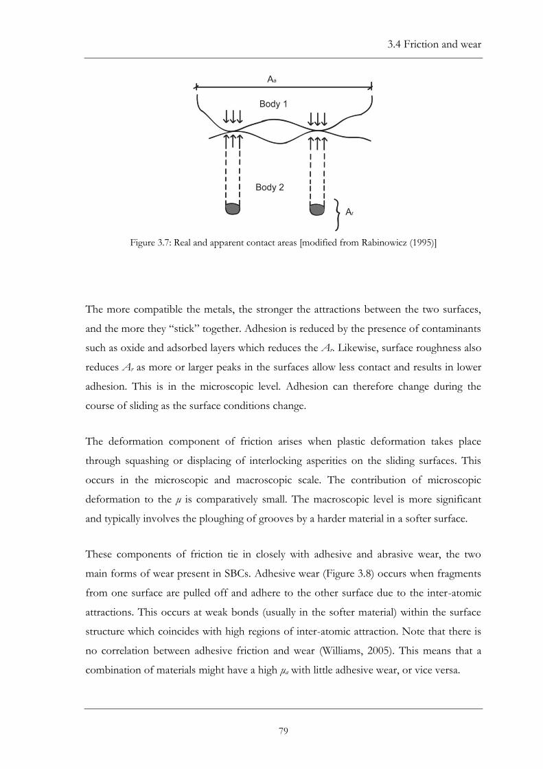
3.4 Friction and wear
79
Figure 3.7: Real and apparent contact areas [modified from Rabinowicz (1995)]
The more compatible the metals, the stronger the attractions between the two surfaces,
and the more they “stick” together. Adhesion is reduced by the presence of contaminants
such as oxide and adsorbed layers which reduces the Ar. Likewise, surface roughness also
reduces Ar as more or larger peaks in the surfaces allow less contact and results in lower
adhesion. This is in the microscopic level. Adhesion can therefore change during the
course of sliding as the surface conditions change.
The deformation component of friction arises when plastic deformation takes place
through squashing or displacing of interlocking asperities on the sliding surfaces. This
occurs in the microscopic and macroscopic scale. The contribution of microscopic
deformation to the μ is comparatively small. The macroscopic level is more significant
and typically involves the ploughing of grooves by a harder material in a softer surface.
These components of friction tie in closely with adhesive and abrasive wear, the two
main forms of wear present in SBCs. Adhesive wear (Figure 3.8) occurs when fragments
from one surface are pulled off and adhere to the other surface due to the inter-atomic
attractions. This occurs at weak bonds (usually in the softer material) within the surface
structure which coincides with high regions of inter-atomic attraction. Note that there is
no correlation between adhesive friction and wear (Williams, 2005). This means that a
combination of materials might have a high μa with little adhesive wear, or vice versa.

Chapter 3: Influence of steel shim hardness on the Sliding Hinge Joint performance
80
The formula governing adhesive wear is V = KNdtravel/H, where V = volume of wear in the
softer material; K = coefficient of wear between the two surfaces; N = normal force; dtravel = total travel
distance; H = hardness of the softer material. The constant K is a measure of the probability of
material being pulled from one surface and adhering to the other and is dependent on the
compatibility of the two sliding materials. Consequently it is lower for unlike materials
and higher for similar materials. This explains the low adhesive wear of half hard
cartridge brass shims, despite having similar hardness to mild steel, whereas the use of
similar metals can cause severe damage with macroscopic tearing of material known as
galling. It is particularly a problem with members of the same material, such as ferrous
alloys (Williams, 2005).
Abrasive wear (Figure 3.9) occurs during friction deformation, and can either be two-
body abrasion where a rough surface ploughs a series of grooves on a softer surface, or
three-body abrasion where abrasive particles are sliding between the opposing surfaces.
This is usually associated with irregular frictional deformation resistance during sliding.
Figure 3.8: Adhesive wear [modified from Rabinowicz (1995)]
Figure 3.9: Abrasive wear [modified from Stachowiak et al. (2005)]

3.4 Friction and wear
81
In terms of the AFC tests, the specimens involved the same softer material (G300 cleat),
and similar N. It is expected that the different grades of steel shims have little difference
in compatibility and therefore the sliding is expected to undergo a similar process. When
sliding first commences, the behaviour is characterised by a low Ar and low friction due
to the presence of surface contaminants. Furthermore, since each surface is initially
smooth, only adhesive friction and adhesive wear are present at this stage. The surfaces
then undergo a process called breaking-in as the cumulative travel increases, where the
contaminants such as oxide layers are removed, and asperities on the opposing surfaces
flatten out. This increases the Ar between the surfaces which increases the adhesion
component of friction. Once breaking-in is complete, the frictional characteristics are
then determined by the mechanical properties and subsequent wear mechanism. While
differences in crystal structure or alloying elements can affect compatibility and hence
frictional resistance, these influences are minimal on altering the coefficient of wear
between the different steel based materials.
The major difference between the shims is thus the material hardness, which is expected
to improve the performance through the reduction of wear. In mechanical engineering
applications, materials are chosen to ensure a difference in hardness between sliding
surfaces. This combination improves frictional performance by allowing the harder
surface to control the interaction and the softer surface to conform. Williams (2005)
states it is common for shafts to be three times harder than the supporting bearing. The
harder material is more wear resistant, which reduces the total adhesive wear over both
surfaces. The difference in hardness also allows hard abrasive particles to imbed in the
softer material. If the particles are completely absorbed, the surfaces are protected, and
the abrasive wear minimised. However, if the particles are only partially embedded, they
may act as aggressive abrasive asperities. With two materials of similar hardness, the
abrasive particles will slide and roll relative to the surfaces resulting in grooving on both
sides through abrasive wear. This is reduced with the different hardness of the two layers.
With a reduction in wear, particularly abrasive wear, the harder shims are expected to
reduce damage, and produce a more stable sliding behaviour.

Chapter 3: Influence of steel shim hardness on the Sliding Hinge Joint performance
82
3.5 Test results
The details and results of the 10 specimens tested are shown in Table 3.2, showing the
expected Vss values calculated from the bolt model in Section 3.3 (Vssn). Each test is
identified by the notation SG.TN for specimens without BeS, and SG.BeS.TN for
specimens with BeS, where SG is the steel grade and TN the test number. All specimens
were tested with newly installed bolts. Specimens G300.BeS, G80.BeS.T2 and
G400.BeS.T2 were conducted using plates from specimens G300.T1, G80.T1 and
G400.T1 respectively. The maximum displacements (Disp) between test specimens varied
as explained in Section 3.3 and are shown in Table 3.2.
The behaviour of each of the different steel shims was characterised by an initial stable
level of sliding friction for the early cycles of loading. This then increased as the
cumulative travel increased, and stabilised at a higher level. This is shown in Table 3.2 as
a force per bolt for the initial stable sliding friction (Vssi) and the stable sliding friction at
the final cycle of maximum displacement (Vssf). Vssi and Vssf are taken at the zero
displacements unless stated otherwise in Table 3.2. The maximum friction per bolt at any
point (Vssm) is also shown. The Vssi, Vssf and Vssm are shown as A, B and C respectively in
Figure 3.10. The R-ratios of Rf/i and Rm/f are a measure of the stability of the force-
displacement characteristics. Rf/i is the ratio of Vssf and Vssi which indicates the level of
increase in sliding friction as the cumulative travel increases. Rm/f is the ratio of Vssm to
Vssf, which indicates the variability of the friction force once breaking-in is complete. A
good combination of materials provides high initial sliding friction (Vssi), stable,
repeatable and predictable force-displacement behaviour and a low increase in friction
over time. These ideal characteristics correspond to high Vssi values and low Rf/i and Rm/f
ratios, which measure the stability of the sliding behaviour.
.

3.5.1 Mild steel shims
83
The experimental values presented are the average of the positive and negative directions.
The negative friction values were consistently larger than the positive values as expected
and described in Section 3.2. On average, the maximum negative friction forces were
8.1% larger than the corresponding positive friction forces. This excludes specimen
G400.T1 where the positive friction was 5.6% larger than the negative friction, and
G80.BeS.T1 where the forces in each direction were approximately the same.
Table 3.2: Test results
Specimen Vssn (kN)
First run Second run
Disp (mm)
Vssi (kN)
Vssf (kN)
Vssm (kN)
Rf/i = Vssf /Vssi
Rm/f = Vssm/ Vssf
Disp (mm)
Vssf
(kN)
G300.T1 91 10.2 62.6 99.8 110.3 1.59 1.11 9.2 100.4
G300.T2 91 9.0 62.3 98.5 113.9 1.58 1.16 8.4 111.5
G300.BeS 111 10.0 82.3b 124.1a 138.7 1.51 1.12 9.7 122.4
G80.T1 91 10.1 66.9a 76.4 93 1.14 1.22 9.8 96.8
G80.BeS.T1 111 9.0 88.4 112.1 115.3 1.27 1.03 12.7 106.9
G80.T2 91 13.9 51.1a 75.8 84.6 1.48 1.12 12.6 86.3
G80.BeS.T2 111 11.9 109.4 118.1 128.4 1.08 1.09 11.9 122
G400.T1 86 15.2 84.1 107.7 110 1.28 1.02 15.7 91.4
G400.T2 86 13.4 89.2 103.4 107.4 1.16 1.04 13 102.9
G400.BeS 104 12.7 106.9 124.5 134 1.16 1.08 12.5 122.5 a Vss did not rise to a stable level at the zero displacement. Values are at stable levels past the zero displacement.
b Friction did not stabilise. Value is at the zero displacement.
3.5.1 Mild steel (G300) shims
Mild steel shims produced the least desirable results with a low initial sliding shear
resistance (low Vssi) and the least stable sliding characteristics (highest R-ratios). This
behaviour was consistent for specimens both with and without BeS.
The two tests carried out without BeS (G300.T1 and G300.T2) had very similar
performance. The friction levels were comparable, with Vssi of 62.6 and 62.3 kN/bolt,
and Vssf of 99.8 and 98.5 kN/bolt respectively. The force-displacement characteristics of
G300.T1 can be seen in Figure 3.10(a). The friction displayed the typical initial stable Vssi
up to the 7 mm amplitude cycles. In the subsequent cycles, which were of amplitudes
exceeding 9 mm, the friction increased with increasing cycles of loading before

Chapter 3: Influence of steel shim hardness on the Sliding Hinge Joint performance
84
stabilising. The increase in friction was the largest amongst the different shims, as
reflected in the largest Rf/i of 1.59 and 1.58 for G300.T1 and G300.T2 respectively. The
friction was also variable once breaking-in was complete, as it was lower while passing
through the zero position, and increased at greater displacements within the same cycle.
This is shown by the Rm/f of 1.11 and 1.16. In the second load regime [shown in Figure
3.10(a) in light blue], the force-displacement behaviour differed with no observed stable
Vssi. Instead, the friction built up and stabilised at the Vssf within a few cycles. The
incremental force behaviour over both dynamic load regimes is shown in the force-
cumulative travel behaviour in Figure 3.11(a). Within the range of total travel, there is no
loss in sliding shear capacity.
The plates from G300.T1 were tested with new bolts and BeS (G300.BeS). The hysteresis
curve and force-cumulative travel are shown in Figures 3.10(b) and 3.11(b) respectively.
The friction was higher as the BeS reduced the loss in bolt tension with a Vssi of
82.3 kN/bolt. While there was generally less variation between cycles, the friction also
increased with increasing cumulative travel, and was also higher at displacements away
from the zero position. This was reflected in the Rf/i and Rm/f of 1.51 and 1.12. In a similar
way to that without BeS, the specimen developed the Vssf within a few cycles in the
second load regime.
The G300 shims did not produce favourable performance, displaying undesirably large
R-ratios. Their use would require a large overstrength factor in design and increase the
overall cost of construction. The behaviour, however, is unlike the sharp initial increases
and quick drop in friction as reported by Grigorian and Popov (1994). This is due to the
asymmetric sliding of the joint (MacRae et al., 2010).

3.5.2 High strength quenched and tempered steel shims
85
3.5.2 High strength quenched and tempered (G80) steel
shims
The use of G80 shims reduced the Vssi and Vssf of the joints, but improved the overall
stability of the sliding behaviour. The combination of G80 shims and BeS were also
tested, which significantly increased the Vssi and sliding stability. It is noted that G80.T1
and G80.BeS.T1 were taken to similar displacements to that of the G300 specimens, while
G80.T2 was taken to the same displacements, followed by three extra cycles of 11.5 mm.
Following tests, starting from G80.BeS.T2, were all taken to five cycles at or close to the
target displacement of 13.8 mm, which corresponds to a joint rotation of 0.030 rad.
The behaviour of the tests conducted without BeS (B80.T1 and B80.T2) was similar to
that of the G300 specimens [Figure 3.10(c)]. This is seen in the characteristic Vssi and Vssf,
and the increase in friction with cumulative travel as shown in Figures 3.10(c) and 3.11(c).
The Vssi and Vssf were lower compared to the G300 specimens, but were more stable with
lower Rf/i ratios, and similar Rm/f ratios. Further increases in friction were shown during
the second dynamic load regime. This could be due to the difference in cumulative travel
over both loading regimes, where the G300 specimens and G80.T2 were taken to
approximately 700 mm and 900 mm respectively. The G80.T2 friction at 700 mm was
similar to the maximum force of the first regime.
It was surprising to notice the slight difference in shape of the hysteresis curve. The
sliding friction built up at a slower rate after load reversal, often only reaching the stable
sliding force after passing the zero position. With the lower friction, and little changes to
the R-ratios, G80 shims do not give a substantial advantage over G300 shims.
Two specimens using BeS (G80.BeS.T1 using new plates and G80.BeS.T2 using plates
from G80.T2) performed significantly better with increased Vssi and Vssf and improved
sliding stability. The force-displacement and force-cumulative travel behaviour of
G80.BeS.T2 are shown in Figures 3.10(d) and 3.11(d). The larger friction forces were a
result of the reduction in bolt tension losses due to the BeS. The R-ratios were also lower
with Rf/i and Rm/f of 1.27 and 1.03 for G80.BeS.T1, and 1.08 and 1.09 for G80.BeS.T2

Chapter 3: Influence of steel shim hardness on the Sliding Hinge Joint performance
86
respectively. The Vssf of G80.BeS.T1 and G80.BeS.T2 were very similar despite the
differences in the initial conditions of the plates. The lower Rf/i of G80.BeS.T2 was
because the plates were reused, resulting in a higher Vssi. A difference was observed in
the specimen behaviour compared to the other tests at load reversal. The force built up
in the expected stepwise manner as the first surfaces slides first, followed by the second
surface. There was then a sudden drop in friction, which was not observed in Clifton
(2005) component tests. The friction then rose to the stable level more quickly than the
specimens without BeS, reaching a maximum before passing through the zero
displacement.
The combination of G80 and BeS gives a significant improvement over G300 shims and
B80 shims without BeS. The sliding capacity is higher, and the behaviour stable with a
low increase in strength, and is therefore easily modelled.
3.5.3 Abrasion resistant (G400) steel shims
The G400 shims produced the best results with the largest and most stable sliding
friction resistance. The results were similar for tests conducted with and without BeS,
with the exception of the increased friction with the BeS.
The force-displacement and force-cumulated travel behaviour of G400.T2 can be seen in
Figure 3.10(e) and Figure 3.11(e). The results were shown to be repeatable with G400.T1
and G400.T2 producing similar results. Both produced higher friction compared to the
other shims, giving a Vssi of 84.1 and 89.2 kN/bolt. There were also significant
improvements in the stability of the sliding behaviour. While there were increases in
friction over time, it was to a much lesser extent than with the G300 and G80 specimens.
These observations are reflected in the Rf/i and Rm/f of 1.28 and 1.02 respectively for
G400.T1, and 1.16 and 1.04 respectively for G400.T2. Note however, that G400.T2 was
the only test that showed a drop in sliding shear capacity in the second loading regime.
Overall, the sliding behaviour is comparable to that of the G80 with BeS specimens.
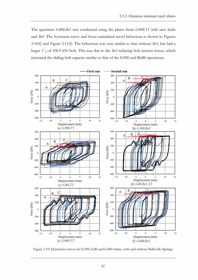
3.5.3 Abrasion resistant steel shims
87
The specimen G400.BeS was conducted using the plates from G400.T1 with new bolts
and BeS. The hysteresis curve and force-cumulated travel behaviour is shown in Figures
3.10(f) and Figure 3.11(f). The behaviour was very similar to that without BeS, but had a
larger Vssi of 106.9 kN/bolt. This was due to the BeS reducing bolt tension losses, which
increased the sliding bolt capacity similar to that of the G300 and Bis80 specimens.
(a) G300.T1
(b) G300.BeS
(c) G80.T2
(d) G80.BeS.T2
(e) G400.T2
(f) G400.BeS
Figure 3.10: Hysteresis curves for G300, G80 and G400 shims, with and without Belleville Springs.
-600
-400
-200
0
200
400
600
-15 -10 -5 0 5 10 15
First run Second run
-600
-400
-200
0
200
400
600
-15 -10 -5 0 5 10 15
Fo
rce
(kN
)
Displacement (mm)
A
B C
-600
-400
-200
0
200
400
600
-15 -10 -5 0 5 10 15
Fo
rce
(kN
)
Displacement (mm)
AB C
-600
-400
-200
0
200
400
600
-15 -10 -5 0 5 10 15
Fo
rce
(kN
)
Displacement (mm)
AB C
-600
-400
-200
0
200
400
600
-15 -10 -5 0 5 10 15
Fo
rce
(kN
)
Displacement (mm)
A B C
-600
-400
-200
0
200
400
600
-15 -10 -5 0 5 10 15
Fo
rce
(kN
)
Displacement (mm)
A
B C
-600
-400
-200
0
200
400
600
-15 -10 -5 0 5 10 15
Fo
rce
(kN
)
Displacement (mm)
A B C

Chapter 3: Influence of steel shim hardness on the Sliding Hinge Joint performance
88
(a) G300.T1
(b) G300.BeS
(c) G80.T2
(d) G80.BeS.T2
(e) G400.T2
(f) G400.BeS
Figure 3.11: Cumulative travel versus force for G300, G80 and G400 shims, with and without
Belleville Springs.
-600
-400
-200
0
200
400
600
0 200 400 600 800 1000
Fo
rce
(kN
)
Cumulative Travel (mm)
-600
-400
-200
0
200
400
600
0 200 400 600 800 1000
Fo
rce
(kN
)
Cumulative Travel(mm)
-600
-400
-200
0
200
400
600
0 200 400 600 800 1000
Fo
rce
(kN
)
Cumulative Travel (mm)
-600
-400
-200
0
200
400
600
0 200 400 600 800 1000
Fo
rce
(kN
)
Cumulative Travel (mm)
-600
-400
-200
0
200
400
600
0 200 400 600 800 1000
Fo
rce
(kN
)
Cumulative Travel (mm)
-600
-400
-200
0
200
400
600
0 200 400 600 800 1000
Fo
rce
(kN
)
Cumulative Travel (mm)

3.5.4 Material wear
89
3.5.4 Material wear
It was observed that the debris being expelled from the sliding surfaces during testing
decreased from G300 to G400 shims. There was also noticeably less debris between the
plates when the specimens were disassembled, indicating a reduction in material wear
with increasing shim hardness. This was reflected in the final surface conditions of the
plates. Figures 3.12 to 3.14 show the typical surface of the shims, cleats and beam flange
plates. Note that these photographs were taken after the removal of loose debris, for
clarity of showing the final surface conditions, and may not correspond to the specimen
graphs in Figures 3.10 and 3.11. Considering the similar force-displacement behaviour in
the second load regime of each of the specimens (Figures 3.10 and 3.11), it can be
concluded that component replacement is not required when any of the shim types are
used. The material wear performance is nevertheless related to the sliding behaviour as
described in Section 3.4.
The G300 specimens exhibited severe damage on both sides of the cleat, and on the
sliding surface of both shims. There was concentrated galling near the bolt holes. Similar
damage was also present on both surfaces of the shim to beam flange plate interface,
albeit to a lesser degree. This was surprising given the little relative movement between
these two surfaces. The conditions of the opposing surfaces were similar as they were the
same material.
There were significant improvements with the use of G80 shims. The surface condition
could be described as moderately scratched, with substantial scratches on both the cleat
and shims. They were more evenly distributed around the sliding surface, as opposed to
the deep, irregular grooves in the G300 specimens. The scratches to the cleat were
slightly deeper compared to the shims, as reflected in the difference in hardness of the
two sliding surfaces. The wear at the shim to beam flange plate interface was insignificant
with the surface showing small, smooth patches with very little material removal.

Chapter 3: Influence of steel shim hardness on the Sliding Hinge Joint performance
90
The G400 specimens showed the least wear. The appearances of the shims were smooth
and shiny as they underwent polishing during sliding. While lines in the direction of
sliding were present, they were well distributed and could not be felt by touch. The cleat
damage was much less compared to the cleat damage when softer shims were used. The
surface roughness of the cleat and shims of the G400.BeS specimen in their final
conditions was measured, and compared to that measured from G400 and G300 steel
plates in their as supplied conditions. The roughness parameter adopted was the Ra
surface roughness, which is the mean height and depth of crests and troughs on the
surface. The measurements were made using a Taylor Hobson Surtronic 3 (Taylor
Hobson, 2013), which measures surface textures to ISO 4287:1997. The G400 shims had
an initial roughness of 7.3 µm and a final roughness of 2.4 µm. The G300 cleat initial
roughness was 2.6 µm, with a final roughness of 1.8 µm. The measurements are an
average of 10 readings taken in the direction of sliding along the lines show in Figures
3.12 and 3.13, at approximately equal distances apart, for a length of 12 mm. These
measurements were not taken for the G300 and G80 specimens as it would not have
given a meaningful result given the extent of damage. This is because Ra measurements
are only suitable for measuring microscopic roughness, as opposed to macroscopic
grooves and galling as described before. It is another indication that surface damage with
the G400 shim and G300 cleat combination is on the microscopic scale rather than the
macroscopic scale.
Figure 3.12: Surface of cleats. Left to right: G300, G80 and G400.

3.5.5 Comparison with bolt model
91
Figure 3.13: Surface of shims. Left to right: G300, G80 and G400.
Figure 3.14: Surface of beam flange plate. Left to right: G300, G80 and G400.
3.5.5 Comparison with bolt model
The bolt model was developed using experimental Vssf values and plastic theory and is
thus compared to the Vssf. The model values proved to be a reasonably good lower
bound prediction of the experimental test values for the 3 mm thick G300 shims. This is
consistent with previous studies (Clifton, 2005, MacRae et al., 2010). It was however not
the case for the G80 shims, which exhibited surprisingly lower Vss values as described
above. The reason for this is unclear.
The Vss measured when G400 shims were used were unexpectedly higher than the
predicted values for 5 mm thick shims. Upon inspection of the bolts from the G400

Chapter 3: Influence of steel shim hardness on the Sliding Hinge Joint performance
92
specimens, it was found from impact marks on the bolts that the loads were transferred
to the bolts through bearing on the shims, as opposed to the cap plate and cleat which is
assumed in the calculation of the lever arm l in the bolt model described in Section 3.2.
This was unique to the G400 shims, and is probably due to the high strength and
hardness resulting in the force transfer being confined to the shims. This effectively
reduced the lever arm and moment demand on the bolt. When the lever arm l is taken as
the thickness of the beam flange plate + thickness of the shim (which corresponds to the distance between
the centroid of the two shims bearing on the bolt), the model predicts a Vss of 119 kN/bolt and
99 kN/bolt with and without BeS respectively. This is a better representation of the
actual conditions during sliding, and moreover gives a better lower bound prediction of
the Vss. It is therefore recommended that a lever arm (l) of beam flange plate thickness + shim
thickness is used in design when G400 shims are used. Note that this recommendation has
been superseded in Section 4.3.2.2. Also please refer to Section 4.3.2.3 for updates to the
bolt model.
3.6 Discussion
The pattern of behaviour showed that the process of wear and friction is similar for each
specimen. This was observed by the lower, initial and stable Vssi during breaking-in,
which increased and stabilised at the Vssf during the first load regime in all specimens with
new plates. This behaviour was not present in the same degree in specimens with reused
plates, or in the second load regimes as breaking-in had already occurred. While the
surfaces would have re-oxidised, it would not be to the same degree within the short time
frame as the tests were conducted within a few days to a week apart. There were
differences in the level of Vssi between the shims showing a difference in the oxide
properties of the shims. The Vssf, however, not only varied significantly between the
different shims in terms of the level of friction, but also the stability. This was due to the
effects of different hardness of the sliding surfaces.

3.6 Discussion
93
In the case of G300 shims, the wear fragments from adhesive wear built up and
eventually formed loose particles which were work-hardened by the sliding motion. Due
to similar surface hardness, three-body abrasive wear then takes place as these hard
particles plough into the opposing surfaces, contributing to μd and increasing the overall
sliding friction. This leads to less predictable patterns of sliding forces as the resistance
became a function of the irregular ploughing friction, on top of the ongoing adhesion
friction and adhesive wear. The resistance also increased due to piling up of deformed
material at the ends of the grooves, which increased the friction at larger displacements.
The material continued to work-harden, which increased the force until it reached a
plateau. This process forms irregular surfaces which leads to an uneven stress distribution
as observed in the concentrated damage.
The use of the harder G80 shims changed the wear mechanism slightly by firstly reducing
adhesive wear on the shims. It secondly reduced the abrasive wear as the harder shims
are only susceptible to the effects of the fewer G80 loose particles adhering to the cleat,
but not to the softer G300 fragments. The difference in hardness allows the hard
abrasive particles to imbed into the softer material. It is believed that only partial
embedment occurred in the cleat, which ploughed the observed scratches in the shims.
Similarly to G300, the increase in friction shear is due to the removal of contaminant
layers and the subsequent deformation component. The latter is significantly reduced,
which results in the smaller increase in friction with cumulative travel as shown by the
lower Vssf compared to the G300 shims. There is also very little increase in friction at
larger displacements, with little piling up of wear particles at the ends of the grooves.
The G400 shims further improved the performance with the highest and most stable
friction force. Compared to G80, the difference in hardness is sufficient to improve the
embedment of hard particles into the softer cleat as observed in minimal wear of the
cleat and shims. This results in stable and consistent friction with little deformation
contributing to the sliding resistance. Despite the lack of deformation friction, the Vssf
was significantly higher. This is a result of the smoother surfaces caused by polishing.
Polishing is a unique form of microscopic abrasive wear by small particles (5 µm or less).
It reduces the surface roughness through the removal of asperities in the microscopic

Chapter 3: Influence of steel shim hardness on the Sliding Hinge Joint performance
94
scale and improves the surface condition (Rabinowicz, 1995). These particles may be
from the oxide layers present in G400. With smoother surfaces, the real contact area
between the plates increases which increases surface attraction and µa.
For each shim tested, it is expected that the friction will eventually drop with further
surface degradation as wear particles between the plates fall out, thereby reducing the
bolt clamping length and normal force. The only test where this was observed was
G400.T1, noting that the specimens were not subjected to the large number of cycles
required for this to occur. This potential drop in capacity is nevertheless insignificant, as
it is unlikely that the joint will be subjected to inelastic deformation as severe as even one
run of the load regime in an actual earthquake. The results have also shown that for each
shim tested, the Vss was independent of the slip rate. This was shown by the stability of
the loop over each individual cycle, and between cycles of different amplitudes. As
described in Section 3.3, the slip rate varies within sinusoidal cyclic loading, as well as
between cycles of different amplitudes. This could be due to the asymmetric sliding
nature which reduces the effects of static and dynamic coefficients of friction as reported
by MacRae et al. (2010) and described in Section 3.4.
The results have shown that, despite the similar material compatibilities, G400 and G300
is a successful sliding pairing in the AFC application, and therefore for the SHJ. It
performed the best with the largest Vssi, the most stable, predictable and repeatable
sliding behaviour, and the lowest increase in sliding shear resistance. While G400 also
performed well with BeS, there appears to be no further improvements compared to the
specimens without them. The only reason for employing BeS would be to minimise losses
in bolt tension over time or through joint sliding. This combination exhibited behaviour
as good as the original component tests by Clifton (2005) using brass shims. There are
considerable benefits of using Grade 400 abrasion resistant steel shims in preference to
brass shims. They are cheaper and more readily available, can be tack welded to the beam
and cleat to facilitate erection, and do not have dissimilar metal issues with corrosion.
Practical design of the joint can be achieved using values computed by the bolt model,
which gives a reasonable lower bound value. They are therefore a preferred solution for
the AFC. It is also recommended that G400 shims are tested in symmetric sliding.

3.7 Summary and conclusions
95
3.7 Summary and conclusions
This paper presented a series of component tests conducted to investigate material
options for shims in asymmetric sliding joints. Grade 300 mild steel, Grade 80 high
strength quenched and tempered steel, and Grade 400 abrasion resistant steel with
measured hardnesses of 168 HB, 266 HB and 382 HB were tested. It was shown that:
1. Adhesion and deformation components of friction were present in
each sliding pair, albeit to different degrees. Adhesion arises from the
inter-atomic attractions between the opposing sliding surfaces.
Deformation is from macroscopic plastic deformation of interlocking
asperities, which results in unstable sliding characteristics.
2. There was no clear correlation between the sliding friction capacity and
increasing hardness. It was highest for G400, followed by G300 and
G80. This was also reflected in the stable friction levels once breaking-
in was complete.
3. G400 had the lowest gain in strength with the lowest Rf/i and Rm/i. This
was followed by G80 and G300 shims.
4. Increasing the difference in hardness of the opposing surfaces
effectively reduces material wear. The wear in G300 shims was the
most severe, followed by G80 and G400. G400 had an improved
surface condition due to polishing. The difference in hardness
minimises adhesive wear on the harder surface, which in turn
minimises abrasive wear on both surfaces. It also allows harder wear
particles to embed into the softer surface which minimises wear on
both surfaces.
5. The G400 produced the most stable hysteretic loops across different
levels of displacement. The behaviour was repeatable with similar
results in the specimens tested. This was followed by G80 and G300,
indicating that harder shims improved the stability despite having
similar material compatibilities.

Chapter 3: Influence of steel shim hardness on the Sliding Hinge Joint performance
96
6. The specimens with G400 performed the best with stable, predictable
and repeatable sliding characteristics. They had the lowest increase in
strength over time enabling the use of lower overstrength factors.
G400 has many advantages compared to brass. It is cheaper and more
readily available, can be tack welded to the beam and cleat to facilitate
erection, and avoids dissimilar metal corrosion issues. Practical design
of the joint can be achieved using values computed by the bolt model,
which gives a reasonable lower bound value. It is therefore a preferred
solution in the SHJ.
7. Belleville springs increase the sliding friction in the AFCs by reducing
the loss in bolt tension. For G300 and G400 shims, they do not give
further improvements in loop stability, but for G80 shims, they
improve the frictional stability. As G400 shims are recommended for
the SHJ (which already produces stable hysteretic behaviour), the only
reason for employing Belleville Springs would be to minimise losses in
bolt tension over time or through joint sliding.
3.8 References
ASTM (2012). ASTM E18: Standard Test Methods for Rockwell Hardness of Metallic Materials,
ASTM International, West Conshohocken, PA, DOI: 10.1520/E0018-12,
www.astm.org .
Bowden, F. P. and Tabor, D. (1950). The friction and lubrication of solids. Clarendon Press,
Oxford.
Chou, C.-C. and Lai Y.-J. (2009). “Post-tensioned self-centering moment connections
with beam bottom flange energy dissipators.” Journal of Constructional Steel Research,
65(10-11): 1931-1941.

3.8 References
97
Christopoulos, C., Filiatrault, A., Uang, C.-M. and Folz, B. (2002). “Posttensioned energy
dissipating connections for moment-resisting steel frames.” Journal of Structural
Engineering, 128(9): 1111-1120.
Clifton, G. C. (2005). “Semi-rigid joints for moment-resisting steel framed seismic-
resisting systems.” Department of Civil and Environmental Engineering,
University of Auckland, Auckland.
Danner, M. and Clifton, C. (1995). “Development of moment-resisting steel frames
incorporating semi-rigid elastic joints.” Report R4-87. Heavy Engineering
Research Association (HERA), Manukau City, New Zealand.
Desroches, R., McCormick, J., and Delemont, M. (2004). “Cyclic properties of
superelastic shape memory alloy wires and bars.” Journal of Structural Engineering,
130(1): 38-46.
Garlock, M. and Li, J. (2008). “Steel self-centering moment frames with collector beam
floor diaphragms.” Journal of Constructional Steel Research, 64(5): 526-538.
Gledhill, S. M., Sidwell, G. K. and Bell, D. K. (2008). “The damage avoidance design of
tall steel frame buildings - Fairlie Terrace Student Accommodation Project,
Victoria University of Wellington.” 2008 NZSEE Conference, Taupo, New
Zealand.
Grigorian, C. E. and Popov E. P. (1994). “Energy dissipation with slotted bolted
connections.” Report No. UCB/EERC-74/02. Earthquake Engineering Research
Centre, Berkeley, California.
International Organization for Standardisation (1997). ISO 4287:1997 Geometrical Product
Specifications (GPS) -- Surface texture: Profile method - Terms, definitions and surface texture
parameters. Geneva, Switzerland.

Chapter 3: Influence of steel shim hardness on the Sliding Hinge Joint performance
98
Iyama, J., Seo, C. Y., Ricles, J. M. and Sause, R. (2009). "Self-centering MRFs with
bottom flange friction devices under earthquake loading." Journal of Constructional
Steel Research, 65(2): 314-325.
Kim, H.-J. and Christopoulos, C. (2008). "Friction damped posttensioned self-centering
steel moment-resisting frames." Journal of Structural Engineering, 134(11): 1768-1779.
Ma, H., Cho, C and Wilkinson, T. (2008). "A numerical study on bolted end-plate
connection using shape memory alloys." Materials and Structures/Materiaux et
Constructions, 41(8): 1419-1426.
MacRae, G. A., Clifton, C., MacKinven, H., Mago, N., Butterworth, J. and Pampanin, S.
(2010)."The Sliding Hinge Joint moment connection." Bulletin of the New Zealand
Society for Earthquake Engineering, 43(3): 202-212.
Ocel, J., DesRoches, R., Leon, R. T., Hess, W. G., Krumme, R., Hayes, J. R. and
Sweeney, S. (2004). "Steel beam-column connections using shape memory alloys."
Journal of Structural Engineering, 130(5): 732-740.
Rabinowicz, E. (1995). Friction and wear of materials. 2nd edition. Wiley, New York.
Ricles, J. M., Sause, R., Garlock M. and Zhao, C. (2001). "Post-tensioned seismic-
resistant connections for steel frames." Journal of Structural Engineering, 127(2): 113-
121.
Ringfeder Gmbh (2008). Damping Technology. Catalogue R60. Krefeld, Germany.
Roeder, C. W. (2002). "Connection performance for seismic design of steel moment
frames." Journal of Structural Engineering, 128(4): 517-525.
Sepúlveda, J., Boroschek, R., Herrera, R., Moroni, O. and Sarrazin, M. (2008). "Steel
beam-column connection using copper-based shape memory alloy dampers."
Journal of Constructional Steel Research, 64(4): 429-435.

3.8 References
99
Solon Manufacturing (2009). Belleville Springs. Catalogue 04-007. Chardon, Ohio.
Stachowiak, G. W. and Batchelor, A. W. (2005). Engineering tribology. 3rd edition. Elsevier
Butterworth-Heinemann, Amsterdam; Boston.
Standards New Zealand (2006). AS/NZS 1252 - High Strength Steel Bolts with Associated
Nuts and Washers for Structural Engineering. Wellington, New Zealand.
Standards New Zealand (2009). NZS 3404 - Steel structures standard. Wellington, New
Zealand, Standards New Zealand.
Taylor Hobson (2013, June 23). Surtronic 3-Plus Handbook. Retrieved 23 June 2013 from
http://www.taylor-hobson.com/uploads/learningzone/user-
guides/Surtronic%203-Plus%20Handbook.pdf.
Williams, J. A. (2005). Engineering tribology. Cambridge University Press, New York.

Chapter 3: Influence of steel shim hardness on the Sliding Hinge Joint performance
100

101
Chapter 4
1 Sliding shear capacity and
residual strength of the
Asymmetric Friction Connection
Further testing on the Asymmetric Friction Connection (AFC) was undertaken once it
was established in Chapter 3 that abrasion resistant steel shims are to be used in future
AFC construction. The experimental tests were carried out in two rounds of testing over
a period of slightly under two years. The first round was from November 2010 to
February 2011, with a focus on determining the residual joint strength (SR) in the AFCs.
The SR is defined as the force required to reinitiate sliding in the softened joint which
determines the post-earthquake joint conditions. This would confirm the need for bolt
replacement in the SHJ bolts following a major shaking in order that the building remains
rigid under other lateral loads such as wind loading, as well as the dependable post-
earthquake contribution of the AFC in the self-centering SHJ (SCSHJ) covered from
Chapter 5 onwards. The results of the first round of testing were reported in Khoo et al.
(2012).

Chapter 4: Sliding shear capacity and residual joint strength of the AFC
102
The results from the first round of testing produced unexpectedly high values of
measured sliding shear capacities (Vss) for M16 and M20 bolts compared to M24 and
M30 bolts, indicating a bolt size effect where smaller bolts have disproportionately larger
Vss. This led to the second round of the test programme which was undertaken from
June to August 2012. The testing and parts of the analysis were carried out by two
undergraduate students (working closely with the author) as part of their honours
research project (Yeung, 2012, Zhou, 2012). The objective was to investigate the
observed bolt size effect, and to determine if the bolt model previously developed to
predict the Vss is representative of the actual connection behaviour. This was achieved
through determining more dependable input variables into the bolt model (ie. coefficient
of friction and lever arm between points of bearing on the bolt), and increasing the AFC
experimental database. It should be noted that as the second round of testing and
analyses were conducted towards the end of the doctoral research programme, the
conclusions and recommendations were unavailable during the testing and analyses of the
other research components in this project (ie. Chapters 5 to 7).
This chapter presents the results and conclusions from both series of tests. While not
representative of the order they were conducted, it was easiest to discuss the bolt
behaviour and sliding shear capacity (Vss), followed by the residual joint strength (SR).
This chapter provides answers to the questions below in the following order:
1. How does the bolt behave during sliding?
2. What are the recommended input parameters (coefficient of friction
and lever arm) in the bolt model to compute the predicted Vss?
3. How representative is the model of the experimentally measured Vss?
4. What is the level of residual joint strength (SR)? Do the bolts need to
be replaced? What is the elastic strength contribution of the AFC in
the post-earthquake joint?

4.1 Introduction
103
4.1 Introduction
4.1.1 Sliding shear capacity (Vss)
The moment resistance in the SHJ is determined by the AFC frictional resistance in the
bottom web and bottom flange, and their respective lever arms from the point of
rotation about the top flange plate. It is therefore calculated as nbfb Vss db + nwbb Vss ewb,
where nbfb = number of bottom flange bolts; Vss = design sliding shear capacity per bolt;
db = beam depth; nwbb = number of bottom web bolts; ewb = distance of the web bottom
bolt group to the point of rotation as described in Section 3.2. As such, the sliding shear
capacities (Vss) for a range of bolt size and cleat thickness are required for its use in
practice. The current values used in design (Clifton, 2007) were determined by a bolt
model previously developed by Clifton (2005) using plastic theory, which was then
modified and presented in MacRae et al. (2010). The bolt model was presented in
Equations 3.1 to 3.5 in Chapter 3, and repeated here for convenience. The computed
design values are provided in Appendix A.
4.1.1.1 Bolt behaviour
The AFC bolts are Property Class 8.8 bolts which are fully tensioned (ie. tightened into
the inelastic range) at installation using the turn-of-nut method in accordance to NZS
3404 (Standards New Zealand, 2009). When sliding commences in the AFC, the bolts are
subject to additional plasticity and the interaction of moment-shear-axial actions (MVP),
which results in an uneven stress distribution through the cross-sectional area of the bolt
and a drop in tension. The stress distribution in the bolt was studied through finite
element analysis (FEA) by Clifton (2005). The FEA model is shown in Figure 4.1, which
consists of the AFC component plates with a single M24 bolt. A displacement controlled
cyclic regime was applied, moving the cleat relative to the beam flange to simulate the
conditions of the AFC during sliding. The changes in bolt tension with respect to slip
between the cleat and beam flange is shown in Figure 4.2. Starting from the point of
initial maximum tension at rest (slightly under 350 kN), there is an initial drop until the
first interface commences sliding in the positive direction. As the displacement increases,

Chapter 4: Sliding shear capacity and residual joint strength of the AFC
104
the tension drops further until the second surface slides. Once both surfaces are sliding,
the bolt tension remains stable till the load reverses at the end of the cycle, which then
drops again as the AFC is pushed in the negative direction. The slight increase in tension
with beam flange axial displacement when both surfaces are sliding is due to prying
effects as the component rotates due to the movement of the column about the pinned
top flange plate. As the load reverses at maximum negative displacement, there is a
further drop in tension, which stabilises and reaches a stable sliding state in subsequent
cycles. The FEA model showed satisfactory agreement with the experimental component
testing (Clifton, 2005). It does not fully take prying effects into account, which occurs
when the cleat is in curvature during large inelastic rotations, however it did investigate
the change in bolt behaviour when the bolt hits the end of the slotted holes, with this
being reported in Clifton (2005).
Figure 4.1: Finite element analysis model of the AFC (Clifton 2005)
Figure 4.2: Bolt tension vs relative slip between beam flange and cleat (Clifton 2005)

4.1.1.2 Bolt model
105
4.1.1.2 Bolt model
The bolt model calculates the Vss based on the theoretical axial tension in the bolt once
the AFC is in the stable sliding state. The bolt at this stage is in double curvature, of
which the external actions, idealised deformation and bending moment distribution in the
bolts are shown in Figure 4.3. The bolt model predicts the Vss with three input
parameters, namely: (1) the coefficient of friction between the opposing surfaces, (2) bolt
size and (3) length of the lever arm between the points of bearing (l). The mathematical
model developed by Clifton (2005) and modified by MacRae et al. (2010) is presented in
Equations 4.1 to 4.5. A factor of 1.12 is applied to the material strength, which is the
ratio of the average bolt tensile strength to the nominal tensile strength (Clifton, 2005).
BMD
R
R
V*
V*l
M*
Cap plate
Bottom flange
Bottom flange
plate
Figure 4.3: AFC idealised bolt deformation, external forces and bending moment distribution
(4.1)
= 𝑁𝜇 (4.2)
= 𝑙
2=𝑁𝜇𝑙
2 (4.3)
= 𝑆 ( − (𝑁
𝑁𝑡 )
𝑐
)𝑓𝑢 ≈ 0. 665𝑑3 ( − (
𝑁
0.56𝑑2𝑓𝑢 )
𝑐
)𝑓𝑢 (4.4)
≈ 0.62𝑓𝑢 0.56𝑑2 (4.5)
where: M* = bolt moment demand; Mrfn = bolt moment capacity considering axial force
interaction; V* = shear force carried by each bolt; Vrfn = bolt shear capacity considering
no axial force interaction; d = nominal bolt diameter; N = bolt tension during sliding;
l = lever arm between points of bearing; Sfn = plastic section modulus of the circular

Chapter 4: Sliding shear capacity and residual joint strength of the AFC
106
core area; c = constant which is taken as 1 or 2, without or with Belleville Springs;
fuf = ultimate tensile stress (830 MPa for Grade 8.8 bolts).
The previously used input coefficient of friction (µ) was 0.30 to 0.35, as recommended by
MacRae et al. (2010). The recommendation was made based on literature applicable for
slip critical joints and the experimental results of SHJ subassembly tests with mild steel
shims. At that time, no experimental testing had been undertaken to determine the µ for
the pairing of mild steel and abrasion resistant steel sliding under the SHJ conditions.
There is likely to be a considerable amount of variability. Values from Kulak et al. (2001)
for slip critical joints gave a mean slip factor of 0.33 with standard deviation of 0.06 for
clean millscale surfaces and a mean of 0.52 with standard deviation of 0.04 for abrasive
blasted surfaces. While the surfaces in the AFC would be sweep blasted as-rolled
conditions in accordance to NZS 3404, it is likely that the surface conditions under stable
sliding would be more similar to abrasive blasted conditions as the millscale would be
worn off during sliding as described in Chapter 3.
The lever arm l is a function of the beam flange plate thickness (tcl). The results from
Section 3.5.5 indicated that the Vss was higher when abrasion resistant steel shims were
used compared to when mild steel shims were used, despite the similar chemical
properties of both ferrous materials. Examination of the bolts indicated that the high
hardness caused the force to be transferred through the shims as opposed to the beam
flange and cap plate when brass or mild steel shims were used. This reduced the lever
arm and increased the Vss. The calculation of the lever arm was modified to l = tcl + tsh,
where tsh = shim thickness (compared to l = tcl + 2tsh +0.2d in Section 1.3.4), which was
shown to compute values comparable to the experimental values of the M24 bolts and tcl
= 16 mm for two specimens without Belleville Springs, and one specimen with Belleville
Springs. The validity for other specimen sizes had yet to be investigated. The purpose of
the round of experimental testing described herein was to determine more dependable
input variables for the µ and l, and increase the AFC experimental database for a range of
specimen sizes likely to be used in practice.

4.1.2 Residual joint strength
107
4.1.2 Residual joint strength (SR)
One of the original objectives of the SHJ was to return to an effectively rigid connection
at the end of the earthquake shaking. As previously described, FEA and experimental
testing of the AFC at the component level and in the SHJ subassembly showed that the
AFC undergoes a permanent loss of elastic strength due to a drop in tension when sliding
occurs. There is insufficient information regarding the post-earthquake joint conditions
as the extent of these losses has not been established. While the hysteretic model
developed empirically in RUAUMOKO (Carr, 2007) models the strength and stiffness
loss behaviour under an earthquake load history, it had yet to be compared to
experimental tests of SHJ or AFC subject to cycles of decreasing amplitudes before
coming to a complete stop, and then pushed till sliding is reinitiated from static
conditions. Testing was therefore required to determine the residual joint strength (SR),
which is defined as the force at which sliding recommences in the post-earthquake joint.
This quantifies the dependable elastic strength in the post-earthquake SHJ, and therefore
the need for bolt replacement. This would also determine the dependable elastic strength
contribution of the AFC in the SCSHJ once subjected to a major earthquake shaking.
4.2 Test description
4.2.1 Test setup
The same test rig used in the experimental testing described in Chapter 3 was used in this
round of AFC component tests. Figure 4.4 shows the overall test setup consisting of the
reaction arm attached to the strong wall with the actuator providing the load at the base.
The AFC specimens consisting of the beam flange plate, cleat, shims and cap plate were
installed at the top of the reaction arm. A typical installed specimen is shown in
Figure 4.5, which also shows the displacement gauges. The top side and bottom (ie. beam
flange plate) side view of a typical specimen is shown in Figure 4.6. There were four bolts
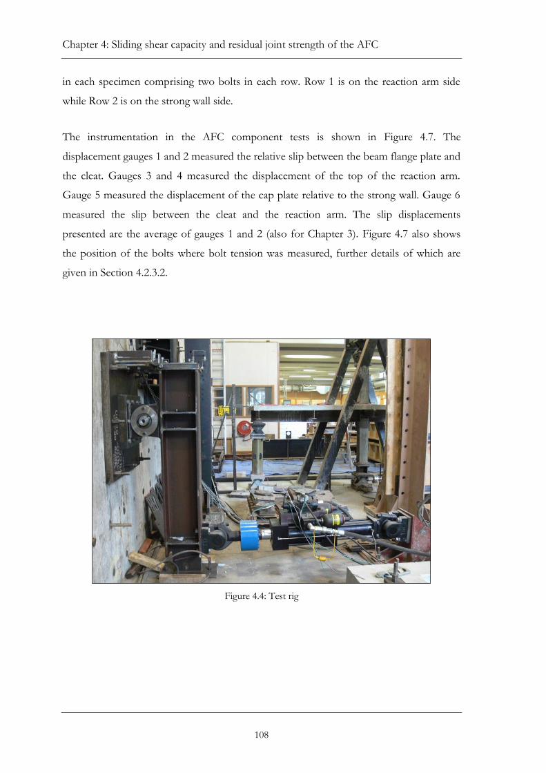
Chapter 4: Sliding shear capacity and residual joint strength of the AFC
108
in each specimen comprising two bolts in each row. Row 1 is on the reaction arm side
while Row 2 is on the strong wall side.
The instrumentation in the AFC component tests is shown in Figure 4.7. The
displacement gauges 1 and 2 measured the relative slip between the beam flange plate and
the cleat. Gauges 3 and 4 measured the displacement of the top of the reaction arm.
Gauge 5 measured the displacement of the cap plate relative to the strong wall. Gauge 6
measured the slip between the cleat and the reaction arm. The slip displacements
presented are the average of gauges 1 and 2 (also for Chapter 3). Figure 4.7 also shows
the position of the bolts where bolt tension was measured, further details of which are
given in Section 4.2.3.2.
Figure 4.4: Test rig

4.2.1 Test setup
109
Figure 4.5: Specimen installed on top of rig with displacement gauges
Figure 4.6: AFC specimen installed with bolt rows indicated. Left to right: top side and bottom (beam flange plate) view

Chapter 4: Sliding shear capacity and residual joint strength of the AFC
110
1
2
56
3
4
M20.16.T3 &
M20.16.T4
M20.16.T5
Bolt tension measurements
Figure 4.7: Instrumentation of AFC component tests
4.2.2 Loading regime
The specimens were tested with two different load regimes. The first (Loading A) was
used in the first round of testing from November 2010 to February 2011, with the aim of
measuring both the sliding shear capacities (Vss) and residual joint strengths (SR) in the
AFC test components. The second (Loading B) was the same regime used in Chapter 3
and was used during the second round of testing from June to August 2012 to measure
only sliding shear capacity. Loading B comprised stepwise increases in displacements of
three cycles each to 3.45 mm and 6.9 mm at 1 Hz, followed by three cycles to 10.35 mm
and five cycles to 13.8 mm at 0.67 Hz.
Loading A comprised a combination of displacement controlled load histories, namely a
dynamic regime (Dy1), quasi-static applied excursions (QEs) and intermediate dynamic
regimes (Dy2). The combination and sequence was developed to determine both Vss and
SR of the test components. The components Dy1, QE and Dy2 of the regime are shown
in Figure 4.8 and described as follows:

4.2.2 Loading regime
111
Figure 4.8: Loading A consisting of Dy1, QE, Dy2, QE and Dy2
Initial dynamic regime (Dy1)
Dy1 was used to determine the Vss under dynamic conditions, while subjecting the test
specimens to the likely total travel, ductility and hence damage that would be expected
under a major earthquake. The test was 3 cycles to 2.3 mm and 3.5 mm, 2 cycles to
4.6 mm, 1 cycle to 6.9 mm and 9.2 mm, 2 cycles to 13.8 mm, and back down again. This
corresponds to rotations of 0.005 rad, 0.0075 rad, 0.010 rad, 0.015 rad, 0.020 rad and
0.030 rad in the SHJ with a 460 UB beam. The regime was adapted from the
recommended testing procedure for steel MRFs by the SAC Joint Venture (2000), which
comprised a series of stepwise increases in drift. The SAC loading was developed through
a series of time-history analyses on 3, 9 and 20 storey frames to determine the expected
DLE demand in steel MRFs. The results from the critical case were then used to develop
a recommended testing regime based on the assumptions that: (1) each cycle causes
damage, (2) damage is cumulative and (3) larger excursions cause greater damage. The
changes from the recommended SAC loading regime are summarised as:
1. The regime was applied in terms of joint rotations as opposed to storey
drifts. Drifts are a combination of column deformation, panel zone
rotation and joint rotation, which the test rig was unable to
accommodate.
-20
-15
-10
-5
0
5
10
15
20
Dis
pa
clem
ent
(mm
)
Time
QE
(either QT or
QC)
≈ 276 sec
Amplitude < 3.5 mm → T = 1 sec/cycle
Amplitude > 3.5 mm → T = 1.5 sec/cycle
T =
1 sec/cycle
Dy2Dy1
T =
1 sec/cycle
QE
(either QT or
QC)
≈ 276 sec
Dy2

Chapter 4: Sliding shear capacity and residual joint strength of the AFC
112
2. The rotational amplitudes were reduced by 0.005 rad from the
specified drifts to take column deformation and panel zone rotation
into account. This was based on the assumption that drifts under 0.5%
are non-damaging (SAC Joint Venture, 2000), which constitutes elastic
deformation in the overall joint assembly, as opposed to inelastic joint
rotation through slip in the AFC.
3. The sequence of excursions was modified from the original stepwise
increase to maximum displacement, to a stepwise increase to maximum
in half the number of cycles and back to minimum with the other half,
followed by a further nine cycles of linearly decreasing amplitudes to
zero. This modification was made to ensure the condition of the
specimen at the end of Dy1 was representative of post-earthquake
conditions. If the joint came to rest immediately after the maximum
excursion, the bolts would be in the sliding state (Figure 4.3), with
different residual joint strengths (SR) in each direction. If the AFC is
then loaded in the same direction as sliding was taking place prior to
stopping, the connection would develop the Vss before sliding re-
commences. If the specimen was loaded in the opposite direction, it
would behave as it does under load reversal, and thus slide at very low
levels of friction. Both of these cases do not represent the actual
conditions of the AFC under earthquake shaking. The stepwise
decreases in cycles ensured the bolts were close to vertical when the
AFC came to a complete stop. Travel and maximum displacement are
the main parameters that affect the level of damage in the AFC. This is
because material wear and degradation increases with travel (Section
3.6), and the level of bolt tension loss is dependent on maximum
displacement (Figure 4.2). By using a combination of cycles (number
and magnitude) that are as similar to the SAC loading as possible, the
regime would reflect the travel, magnitude and number of cycles under
a DLE, and thus also the expected cumulative damage.

4.2.2 Loading regime
113
Quasi-static excursion (QE)
Dy1 was followed by a QE loading, which is an excursion to an AFC displacement of
approximately 4.6 mm, corresponding to a rotation of 10 mrad in the SHJ. It was applied
at a slip rate of 1 mm/minute at the specimen level, which gives a definite point where
sliding recommenced in the AFC, and hence the residual joint strength (SR). The
displacement QE can be either a tension load (QT) or compression load (QC),
representing positive (column rotating away) or negative (column rotating in) joint
rotations in the SHJ respectively.
Intermediate dynamic loading (Dy2)
Following the QE, the intermediate dynamic regime (Dy2) was applied to ensure the AFC
winds down and the bolts are close to vertical in a similar way to the Dy1 regime. The
number of excursions was arbitrary, and consisted of five cycles each to 3.5 mm and
2.3 mm, followed by nine cycles of decreasing amplitudes. Following this, the QE was
applied again, this time in the opposite direction to the initial QE.
The procedure was repeated till each specimen was tested a total of four times, with two
of each QT and QC to maximise the number of data points. An example of a complete
regime therefore consisted of an initial Dy1, followed by QT, Dy2, QC, Dy2, QC, Dy2 and
QT. The tension and compression QE (ie. QT and QC) were used interchangeably, but
with always two of each per specimen. In reality, the AFC sliding surfaces would undergo
further wear which would reduce the clamping length, and hence bolt tension and
friction. The later tests were thus expected to yield lower SR due to the additional travel
from the QE and intermediate dynamic (Dy2) loadings. However, as there was no
noticeable difference between the earlier and later SR of the same specimen, it was
concluded that the additional travel was insufficient to alter the SR and all tests were
representative of post-earthquake joint conditions. No AFC specimens were tested with
load histories typical of earthquake shaking (eg. time-history outputs). This was
undertaken for the large-scale SHJ tests described in Chapter 6.

Chapter 4: Sliding shear capacity and residual joint strength of the AFC
114
4.2.3 Test specimens
4.2.3.1 Specimen sizes
A total of 69 tests were conducted, consisting of M16, M20, M24 and M30 bolts, with
cleat thicknesses of 12, 16, 20 and 25 mm. They were chosen to provide a range of sizes
likely to be used in practice. Only M24 bolts were tested with Belleville Springs, where
each bolt was installed with three 16M168 springs in parallel with a combined flat load of
184 kN (Solon Manufacturing, 2009). The specimen details are summarised in Table 4.1,
which provides details of bolt size, cleat thicknesses, loading regime and number of tests.
The naming system adopted is bolt_size.cleat_thickness.test_number for specimens without
Belleville Springs, and bolt_size.cleat_thickness.BeS.test_number for specimens with Belleville
Springs. The tests numbering starts with specimens under Loading A followed by
Loading B. For example, for specimens with M16 bolts and 12 mm thick cleat, 5
specimens were tested with 2 under Loading A (M16.12.T1 and M16.12.T2) and 3 under
Loading B (M16.12.T3 to M16.12.T5). The effects of bolt clamping (grip) length on the
Vss were also studied with clamping lengths varying from 63 to 95 mm in the M20 bolts
with 16 mm thick cleat specimens (ie. M20.16.T1 to M20.16.T17). The clamping lengths
consisted of the beam flange plate, cleat, cap plate, shims and stacked washers to make
up the required lengths. No correlation was found between Vss and clamping length, and
therefore the results are presented assuming all bolt lengths are the same. Further details
of the independence of Vss on the bolt lengths can be found in Yeung (2012).
New bolts were used in each test, while some of the cleats and shims were reused. For
the tests under Loading A, a comparison was made between the performance of
specimens with unused, as-rolled surface conditions, and specimens which had already
been tested and therefore subject to wear. It was found that there was no difference in
the Vss once breaking-in had occurred. Consequently all specimens were considered to be
representative of actual SHJ conditions, with tests under Loading B generally using shims
that had previously been used and subjected to wear and breaking-in of the surfaces. The
dimensions of the plates used for each specimen size can be found in Appendix A.

4.2.3.2 Bolt tension tests
115
Table 4.1: Details of AFC test specimen
Specimen name Details Number of tests
Bolt Cleat Loading A Loading B Total
M16.12.T1 – M16.12.T5 M16 12 2 3 5
M16.16.T1 – M16.16.T4
16 2 2 4
M16.20.T1 – M16.20.T2
20 2 - 2
M20.12.T1 – M20.12.T5 M20 12 2 3 5
M20.16.T1 – M20.16.T171
16 4 13 17
M20.20.T1 – M20.20.T8
20 2 6 8
M24.12.T1 – M24.12.T4 M24 12 4 - 4
M24.16.T1 – M24.16.T82
16 3 5 8
M24.20.T1 – M24.20.T5
20 2 3 5
M30.20.T1 M30 20 1 - 1
M30.25.T1 – M30.25.T2
25 2 - 2
M24.12.BeS.T1 – M24.12.BeS.T2 M24 12 2 - 2
M24.16.BeS.T1 – M24.16.BeS.T32 16 2 1 3
M24.20.BeS.T1 – M24.20.BeS.T3 20 3 - 3 1 Includes strain gauged and load cell specimens described in Section 4.2.3.2 below (M20.16.T3 – M20.16.T5)
2 Includes test results from Chapter 3, where G400T1, G400T2 and G400.BeS renamed as M24.16.T4, M24.16.T5 and M24.16.BeS.T1 respectively
4.2.3.2 Bolt tension tests
An attempt to determine the coefficient of friction (µ) was made by measuring the
tension (N) in the bolts with strain gauges installed in the shank, and a load cell under the
bolt head when sliding was taking place. The measurement of bolt tension also provided
experimental validation of the predicted bolt behaviour during sliding. The specimens
were identical and comprised M20 bolts and 16 mm thick cleats and were subjected to
Loading B. The specimen names were M20.16.T3 to M20.16.T5.
The 4 bolts in specimen M20.16.T3 were installed with strain gauges. The M20 bolts were
110 mm long comprising threaded and shank lengths of 53 and 57 mm respectively. The
strain gauge model was KFG-1.5-120-C20-11, installed with EP-180 adhesive (Kyowa
Electronic Instruments, 2012). The strain gauges were inserted into Ø2 mm holes that
were drilled into the middle of the bolt head. The depth of the hole was 42 mm past the
end of bolt head, which is a relatively uniform area and free from end-effects. The strain
gauge readings from each bolt was then calibrated with a washer type load cell by
tightening the bolts to snug tight, which is within the elastic range of the bolts. As the
shank would theoretically be elastic in the fully tensioned state (assuming any inelastic

Chapter 4: Sliding shear capacity and residual joint strength of the AFC
116
deformation occurs in the threads), this would provide a reasonable measurement of the
bolt tension at installation. The bolts would then be subject to the uneven stress
distribution during sliding, which may cause the readings from the strain gauge to be
unrepresentative of the actual bolt tension. This may be mitigated by the installation of
the strain gauge in the middle of the bolt, which is the theoretically neutral axis.
However, only one bolt from M20.16.T3 produced meaningful measurements during
AFC sliding. The position of the bolt is shown in Figure 4.7. The load cell model was
LWO-60 from Transducer Techniques, Temecula (Transducer Techniques, 2012), which
was purchased for this project and calibrated by the manufacturer prior to delivery. The
load cell measurement was also verified with calibrated load cells to ensure dependability.
The bolt which produced meaningful strain gauge readings was reused in the same
position in specimen M20.16.T4, with the LWO-60 load cell installed under the bolt head
to determine the accuracy of the strain gauge measurements. The other bolts were also
from the M20.16.T3 specimen to maintain consistency. The tension could only be
measured in one bolt at any one time as only one suitable washer load cell was available.
The same set of bolts were again used in specimen M20.16.T5, except the working strain
gauge bolt was placed in the row of bolts closer to the strong wall (Row 2) to determine
any row effects (the position shown in Figure 4.7).
There are limitations to the two methods of bolt tension measurement. The provisions of
NZS 3404 do not allow bolts to be reused just once after they have been fully tensioned.
The performance may differ from that expected from unused bolts, as they would have
been pushed further into the inelastic plateau. It should also be noted that the drilled
holes in the bolt head and shank as well as the washer shaped load cell are variations
from that expected in construction and may influence bolt performance. Furthermore,
upon consultation with the load cell manufacturers, it was advised that uniform load
distribution from flat surfaces at each side was required for accurate measurements. This
was the case during bolt tensioning, at which point the correct functioning of the load
cell was checked. However, it is not the case for the AFC when the bolts are in double
curvature. The tests were nevertheless conducted to provide two independent
measurements of bolt tension.

4.3 Results and discussion
117
4.3 Results and discussion
The test results are presented in the following order: (1) behaviour of the AFC in the
strain gauged/load cell tests, (2) input parameters and modification to the bolt model, (3)
sliding shear capacities and (4) residual joint strengths.
4.3.1 Strain gauge/load cell tests
4.3.1.1 Evaluation of bolt tension measurements
Figure 4.9 presents the bolt tension (N) for the single bolt in Row 1 from M20.16.T4, and
the bolt from Row 2 in M20.16.T5 respectively. The N throughout the whole testing
duration, from tensioning through to sliding is shown in Figure 4.9(a) and (b). The
tensioning process of the bolt represents uniform load distribution, which is the
recommended usage of the load cell. As mentioned in Section 4.2.3.2, the load cell was
purchased for this project and calibrated by the manufacturer prior to delivery. The
measurements were also verified with a calibrated load cell to ensure reliability.
Under snug tight conditions, there were discrepancies of about 35% in the M20.16.T4
bolt tension measurements, with the strain gauge and the load cell reading approximately
47 kN and 35 kN respectively. When fully tensioned with the part-turn method, the
strain gauge read approximately 144 kN, and was reasonably stable till sliding
commenced. The load cell initially read approximately 130 kN, which then increased and
stabilised at approximately 144 kN. The stabilisation of the reading in the load cells was
also observed during trials of the load cells, and may limit the accuracy of the results
during sliding. In M20.16.T5, the strain gauge reading of 31 kN was almost double the
load cell reading of 17 kN at snug tight. When fully tensioned and stabilised, the strain
gauge and load cell recorded 119 kN and 114 kN respectively, which is a difference of
approximately 5%. In both specimens, the strain gauge and load cell produced similar
pattern of behaviour when the bolt was being tensioned. The results therefore indicate
that at low levels of load, the difference in the readings was high at 35% or more, while at

Chapter 4: Sliding shear capacity and residual joint strength of the AFC
118
high loads (fully tensioned), the values were within 5%. The readings of the two systems
were more closely matched if the component was allowed to stabilise with time.
The results from the strain gauge and load cell in M20.16.T4 and M20.16.T5 during
dynamic testing are shown in Figure 4.9(c) and (d). The strain gauge and load cell again
produced similar pattern of behaviour. However as expected, there were discrepancies in
the measured bolt tensions, with the accuracy limited by the strain gauge and load cell
measurements described above. The bolt tension readings are covered in more detail in
Section 4.3.1.2.
Figure 4.9: Comparison between strain gauge and load cell readings in M20.16.T4 (bolt in Row 1) and
M20.16.T5 (bolt in Row 2)

4.3.1.2 Bolt behaviour
119
4.3.1.2 Bolt behaviour
The measured Vss, taken as the resistance at the final cycle of maximum displacement
(Vssf in Chapter 3) for specimens M20.16.T3 to M20.16.T5 were similar at 60 kN/bolt,
65 kN/bolt and 60 kN/bolt respectively. Figure 4.10 presents their force-displacement
curves, where positive represents loading in tension (ie. positive joint rotation or column
rotating away). The M20.16.T3 curve was similar to that described in Chapter 3, where
the Vss stabilised and remained constant, with negligible difference between the initial
sliding shear resistance when sliding first commenced (Vssi) and Vssf. This was not
unexpected as the shims and cleat had been used in previous tests, and therefore had
already been subject to wear and breaking-in of the surfaces. M20.16.T4 and M20.16.T5
displayed a different behaviour, where the Vssi was initially higher at 86 kN/bolt and
85 kN/bolt respectively, which then dropped to Vssf. This could be due to the use of
recycled bolts, which would have undergone further strain hardening and resulted in
higher strengths. The specimens nevertheless had similar Vssf, corresponding to the stable
sliding state, which is the focus of the bolt model and this study. The Vss referred to from
here is the Vssf.
Figure 4.10: Hysteretic behaviour of strain gauged tests (M20.16.T3, M20.16.T4 and M20.16.T5)
-150
-100
-50
0
50
100
150
-15 -10 -5 0 5 10 15
Sli
din
g s
hea
r (k
N/b
olt
)
Displacement (mm)
M20.16.T3
M20.16.T4
M20.16.T5

Chapter 4: Sliding shear capacity and residual joint strength of the AFC
120
The tests with strain gauges and load cells used to measure the tension in the bolts while
sliding have been discussed in Section 4.3.1.1. While the actual measurements from the
strain gauge and load cell (shown in Figure 4.9) are not fully consistent with each other,
taken together, they provide a reasonable representation of the bolt behaviour when
sliding is taking place. Figures 4.11 and 4.12 present the bolt tension with respect to the
AFC slip for specimens M20.16.T3, M20.16.T4 and M20.16.T5. The graphs present the
results with just the strain gauge reading for M20.16.T3, and both load cell and strain
gauges for M20.16.T4 and M20.16.T5.
The bolt in M20.16.T3 (Figure 4.11) was tensioned to only approximately 60 kN, which is
significantly lower than that expected for an M20 bolt. This could be due to an error in
the strain gauge reading (no load cell reading taken to verify), or the bolt was not fully
tensioned despite the part-turn tensioning process. Consequently, the drop in bolt
tension as first sliding commences (as indicated in the FEA study shown in Figure 4.1)
was not observed. Instead, the bolt tension increased between the pre-sliding and the
post-sliding states. The reading however illustrates the bolt behaviour in the stable sliding
state, seen clearly during cycles at the maximum amplitude of approximately 10 mm
(shown in Figure 4.11). A typical cycle is described starting from the point at zero
displacement while in the stable sliding state (shown as A). At this stage, sliding on both
interfaces is engaged and the bolt is in the stable, double curvature state. The bolt tension
increases as the AFC is pushed in the positive direction and away from the plumb
position, which is due to prying effects as the cleat bends around the beam flange plate.
The bolt tension peaks at the maximum displacement (shown as B) before the load is
reversed. The bolt tension then drops (shown as C), which corresponds to the point the
bolt has been pushed back from its double curvature shape and is near vertical. This is
unlike the expected behaviour from the FEA (Figure 4.1), but is consistent with the drop
in Vss at load reversal and the pinched hysteretic curve shape. As the load is then
increased in the negative direction, the bolt is pushed to its double curvature state in the
opposite direction. This causes the tension and resulting Vss to increase. The tension and
Vss then plateaus as the bolt reaches the stable double curvature state (shown as D).

4.3.1.2 Bolt behaviour
121
Figure 4.11: Bolt tension vs AFC displacement for M20.16.T3 (strain gauge reading)
The behaviour of the bolt in M20.16.T4 [shown in Figure 4.12(a)] was the most similar to
that expected from the FEA model (Clifton, 2005). The bolt had an initial installed
tension of 144 kN as previously described. As it was first subjected to sliding, the tension
was reasonably constant at low displacement amplitudes up to approximately 0.6 mm.
When the amplitude increased to 3.5 mm (in the positive direction), there was a
permanent drop in tension when the load reversed, which continued to decrease over the
three cycles to 3.5 mm. There was then a significant drop in tension as the amplitudes
increased from approximately 3.5 mm to 7.5 mm. When the amplitude increased to
approximately 13 mm, the bolt tension stabilised with repeated cycles. Once the stable
sliding state had been reached, the bolt behaviour was similar to that described for
M20.16.T3 above. However, the bolt tension was higher when loading in the positive
direction and plateaued at approximately 80 kN compared to 70 kN in the negative
direction for the strain gauge readings. The load cell also produced the same pattern of
behaviour where the bolt tensions in the positive and negative directions were 73 kN and
57 kN respectively. The higher tension in the positive direction was unexpected given
was no difference in the positive or negative Vss. This is also inconsistent with the
0
20
40
60
80
100
120
140
160
-15 -10 -5 0 5 10 15
Bolt
ten
sion
(kN
)
Displacement (mm)
Initial cycles
Maximum amplitude cycles
A
BD
C

Chapter 4: Sliding shear capacity and residual joint strength of the AFC
122
behaviour of M20.16.T3, where there was no noticeable difference between the positive
and negative bolt tension (Figure 4.11). The difference under positive and negative
loading is due to prying effects described below.
The bolt in M20.16.T5 had similar overall behaviour with M20.16.T4 from the strain
gauge reading. From the installed bolt tension of approximately 119 kN, the tension
decreased with increasing cycles and amplitude. The bolt tension eventually stabilised at
70 kN and 50 kN in the positive and negative directions respectively. However, the load
cell gave an unrealistically large bolt tension reading of 110 kN during stable sliding in the
positive direction. In the negative direction, the load cell gave near identical readings with
the strain gauge of approximately 50 kN. The load cell measurement was also
characterised by an increase in tension at load reversal, which then dropped significantly
before building up again. This was observed to a lesser degree in M20.16.T4. The
behaviour is inconsistent with the hysteretic behaviour of the AFC, and also the strain
gauge reading. It is probably due to the limitations of the load cell reading the uneven
load distribution in the bolts under the AFC sliding conditions.
Figure 4.12: Bolt tension vs AFC displacement (slip)

4.3.1.2 Bolt behaviour
123
Overall from all three tests, the strain gauge and load cell readings showed bolt behaviour
similarities with the FEA model in Clifton (2005). The primary difference was the
significant drop and increase in tension that occurred after load reversal as the bolt was
pushed from double curvature in one direction to double curvature in the other direction.
The results also indicate that there may be a difference between the positive and negative
directions. This observation could be due to prying effects which were not fully taken
into account in the FEA model.
The prying effects in the AFC under both positive and negative rotational conditions are
illustrated in Figure 4.13. When loaded in the positive direction, the cleat bends around
the beam flange plate causing an uplifting effect which is more severe further from the
edge of the beam flange. While the bolt tension may increase, the effective normal force
between the plates may decrease due to the uplifting effect, which would result in a lower
Vss. In the negative direction, the cleat is pushed down onto the beam flange plate. There
is however no increase in overall normal force and Vss as it would be balanced by a
decrease in clamping length and bolt tension. As the strain gauge and load cell readings
measure bolt tension rather than normal force, this may be the cause of the larger tension
measurements when loaded in the positive direction compared to the negative direction.
This is also consistent with previous studies (Clifton, 2005, MacRae et al., 2010) and in
Chapter 3, where it was found that the Vss in the negative direction is slightly higher than
in the positive direction.
The prying effect may lead to increased demands and inelastic action in the bolts, and
overall loss in tension. The uplifting effect is more severe for bolts further from the edge
of the beam flange plate (in this case Row 2), which may have caused the differences in
the load cell readings between M20.16.T4 and M20.16.T5, corresponding to the
behaviour of bolts in Row 1 and Row 2 respectively. This would suggest that the loss in
bolt tension and hence Vss may be influenced by the number of bolt rows. More rows
may reduce the overall impact of prying on the individual bolts as prying is resisted by a
larger number of bolts over a longer connection. The effect of the number of rows on
the Vss has yet to be investigated and is recommended for future research.

Chapter 4: Sliding shear capacity and residual joint strength of the AFC
124
Row 1Row 2
Positive rotation
(tension loading)
Negative rotation
(compression loading)
Direction of motion
Direction of motionRow 1Row 2
Figure 4.13: Prying of the AFC under positive (tension) and negative (compression) loading
4.3.2 Bolt model
4.3.2.1 Coefficient of friction (µ)
The results of M20.16.T3 to M20.16.T5 were used to determine an estimate of the
coefficient of friction (µ) between the mild steel cleat and the abrasion resistant steel
shims. This was achieved by calculating µ = Vss/2N, where Vss is the frictional resistance
per bolt (ie. the total measured resistance of the test specimen divided by 4 bolts), while
the factor of 2 takes the two sliding interfaces of the AFC into account.
Figure 4.14 plots the Vss/2N with respect to time for M20.16.T3 to M20.16.T5. This is
presented for just the strain gauge reading in M20.16.T3, and both strain gauge and load
cell readings in M20.16.T4 and M20.16.T5. Note that the extreme values in M20.16.T5
due to the load cell reading large decreases at load reversal from the positive direction
were removed. In each of the specimens, the Vss/2N started at a level of 0.1 to 0.2 in
both the positive and negative directions apart from the positive M20.16.T3. The Vss/2N
then increased and stabilised at higher levels of amplitude. This behaviour does not
reflect the actual µ as the AFC in the initial state was characterised by unstable bolt
tension and low level displacements where both sliding interfaces may not have been

4.3.2.1 Coefficient of friction
125
sliding at the same time. The most appropriate location to determine µ is when the bolt is
in the stable sliding state in double curvature during cycles to the largest amplitude
displacement, corresponding to the stable plateaus in bolt tension (Figure 4.11 and 4.12).
There were variations between the strain gauge and load cell readings between repeated
cycles to the same displacement and between positive and negative directions. The
discrepancies in the measurements were due to uncontrollable factors described
previously such as prying effects and strain gauge or load cell limitations. A µ value was
therefore determined for both the positive and negative directions at the point of greatest
consistency in each specimen. For M20.16.T4 and M20.16.T5, it was also attempted to
adopt the µ where the strain gauge and load cell recorded the most similar bolt tension.
The values are shown in Figure 4.14 and summarised in Table 4.2. The average over the
three specimens in both positive and negative directions is µ = 0.48, which is
recommended for use to compute the Vss. This is significantly higher than the µ = 0.30
previously adopted, but is more similar to the mean slip factor of 0.52 for abrasive
blasted surfaces in slip critical joints from Kulak et al. (2001). Abrasive blasted surfaces
are more representative of surfaces subjected to wear compared to clean as-rolled surface
conditions. The value of µ = 0.48 is therefore recommended to calculate the Vss in the
bolt model.
The reliability of the experimentally determined µ is limited by the test data, where only
three tests were undertaken, and the assumptions in the calculations. The tension was
only measured in one bolt, whereas each specimen comprised four bolts. There would be
variability in tension due to material properties as well as between bolt rows due to
prying. The tests were also conducted using reused shims and cleats as opposed to the
as-rolled surfaces used in practice which may add additional variability to the system and
test results. It is recommended that further studies are undertaken to determine a more
reliable co-efficient of friction.

Chapter 4: Sliding shear capacity and residual joint strength of the AFC
126
(a) M20.16.T3 (Row 1)
(b) M20.16.T3 (Row 1)
(c) M20.16.T4 (Row 2)
Figure 4.14: Vss/2N vs time for strain gauged tests (M20.16.T3, M20.16.T4 and M20.16.T5)
Table 4.2: Summary of results from coefficient of friction tests
Specimen Vss
(kN/bolt)
Coefficient of friction (µ)
Positive direction
Negative direction
Average
M20.16.T3 60 0.37 0.42 0.40
M20.16.T4 65 0.50 0.55 0.53
M20.16.T5 60 0.48 0.55 0.52
Average 61.7 0.45 0.51 0.48
-0.6
-0.4
-0.2
0
0.2
0.4
0.6
0 5 10 15 20 25 30
Vss
/2N
Time (s)
µ = 0.37
µ = 0.42-0.8
-0.6
-0.4
-0.2
0
0.2
0.4
0.6
0.8
590 595 600 605 610 615 620
Vss
/2N
Time (s)
Strain gauge
Load cell µ = 0.50
µ = 0.55
-1
-0.8
-0.6
-0.4
-0.2
0
0.2
0.4
0.6
0.8
440 445 450 455 460 465 470
Vss
/N
Time (s)
Strain gauge
Load cellµ = 0.48
µ = 0.55

4.3.2.2 Lever arm
127
4.3.2.2 Lever arm (l)
The marks on bolts from each specimen were examined at the end of each test to
determine the points of impact with the plates and hence the length of the lever arm (l).
The examination was made for not just the strain gauge and load cell tests, but for the
other tests described in Sections 4.3.3 and 4.3.4 below in order to verify the observation
in Section 3.5.5 in Chapter 3 that the lever arm between points of bearing is from shim to
shim. As a result of that observation, the calculation of the lever arm was modified from
cleat thickness + 2×shim thickness + 0.2×bolt diameter (l = tcl + 2tsh + 0.2d) presented in
Section 1.3.4, to cleat thickness + 2 × shim thickness (l = tcl + tsh).
It was found to be variable between test specimens with no correlation between bolt size
or cleat thickness. The points of bearing were also often smeared over the location of the
shims and the bottom flange plate or cap plate, making it difficult to determine fully
where the load was transferred. There was also variability whereby the points of bearing
were different on either side of a bolt, indicating different lever arms in either direction.
Based on a general observation, a majority of the marks indicated that the point of
impact occurred at the beam flange-shim and cap plate-shim interfaces. It was thus
decided that the recommendations from Section 3.5.5 should be modified to the
calculation of the lever arm as l = tcl + 2 × tsh where tcl = cleat thickness; tsh = shim
thickness. This corresponds to approximately the average between the lever arm adopted
by Clifton (2005) and MacRae et al. (2012), and that recommended in Section 3.5.5. As
this recommendation is based on a general observation rather than a quantitative
measurement, it may be subject to change and should be used with caution. Further
testing and observation is required to determine a lever arm value with greater certainty.

Chapter 4: Sliding shear capacity and residual joint strength of the AFC
128
4.3.2.3 Effective bolt area
Prior research (Clifton, 2005; MacRae et al., 2010) computed the bolt strengths using the
area of the shank. The actual performance will however be determined by where the load
is applied, either shank or threaded region. The bolts were installed in the AFC with the
bolt head on the beam flange plate side for all tests which led to the bearing location of
the beam flange side always being the shank. The second point of impact on the cap plate
side was then dependent on the bolt length and clamping length. Examination of the
bolts indicated that both points of bearing were generally in the shank for M16 and M20
bolts. For M24 and M30 bolts, the points of bearing on the beam flange plate side were
on the shank, while the points of bearing on the cap plate side were generally on the bolt
threads. A simplified method to incorporate this possible influence by using the average
strengths of the shank and threads is presented in Equations 4.6 and 4.7, which should be
used in place of Equation 4.1 for M16 - M20 bolts and M24 - M30 bolts respectively,
with Equations 4.2 to 4.5 remaining the same. The proposed modification would reduce
the predicted strength and could be the cause for the bolt size effect observed previously
where small bolts have a disproportionately larger capacity compared to larger bolts.
(
) (
) (4.6)
(2
𝑡 ) (
2
𝑡 ) (4.7)
where: M* = bolt moment demand; Mrfn,shank = bolt shank moment capacity considering
axial force interaction; Mrfn,thread = bolt thread moment capacity considering axial force
interaction; V* = shear force carried by each bolt; Vrfn,shank = bolt shank shear capacity
considering no axial force interaction; Vrfn,thread = bolt thread shear capacity considering
no axial force interaction

4.3.3 Sliding shear capacity
129
4.3.3 Sliding shear capacity
The average values for the different specimen sizes without and with Belleville Springs
are presented in Tables 4.3 and 4.4 respectively, showing the bolt size, cleat thickness (tcl);
computed strength from the bolt model (Vss,cal); experimentally measured strength
(Vss,exp); ratio between measured and computed strengths (Vss,exp/Vss,cal) presented as the
mean for each specimen type and mean, standard deviation (Ω) and 95th percentile for
each bolt size group and overall sample. The The Vss,cal is computed by the bolt model
using Equations 4.2 to 4.5, and Equation 4.6 for the M16 and M20 bolts and Equation
4.7 used for M24 and M30 bolts. The Vss,exp is the strength at zero displacement in the
final cycle of maximum amplitude.
Table 4.3: Average test results for AFCs without Belleville Springs
Bolt tcl
(mm) No.
Vss,cal (kN/bolt)
Vss,exp (kN/bolt)
Vss,exp/Vss,cal
Specimen mean
Bolt size group
Mean Ω 95th percentile
M16
12 5 49.5 46.9 0.95
1.02 0.15 0.81 16 4 45.5 46.0 1.01
20 2 42.2 50.0 1.18
M20
12 5 85.8 79.5 0.93
0.91 0.16 0.73 16 17 79.5 69.8 0.88
20 8 74.1 72.4 0.98
M24
12 4 116.7 122.8 1.05
1.00 0.11 0.83 16 8 108.5 113.4 1.05
20 5 101.5 92.4 0.91
M30 20 1 177.0 125.0 0.71
0.76 0.04 0.71 25 2 165.1 129.4 0.78
Overall*
0.95 (0.96)
0.16 (015)
0.73 (0.75)
* Values in brackets excludes M30 bolts
Table 4.4: Average test results for AFCs with Belleville Springs
Bolt tcl
(mm) No.
Vss,cal (kN/bolt)
Vss,exp (kN/bolt)
Vss,exp/Vss,cal
Specimen mean
Bolt size group
Mean Ω 95th percentile
M24
12 2 137.3 131.3 0.96
1.01 0.05 0.93 16 3 128.0 131.0 1.02
20 3 120.0 125.3 1.04

Chapter 4: Sliding shear capacity and residual joint strength of the AFC
130
The model predicts a trend of decreasing strength with increasing tcl and ln. This is
because the moment demand in the bolt increases as the lever arm increases, which in
turn reduces the axial force and Vss. The effective coefficient of friction (µn) with respect
to the lever arm normalised by the bolt diameter (ln) for the AFC without Belleville
Springs is shown in Figure 4.15. The µn is Vss/2Nthe which is the Vss normalised by twice
the theoretical installed bolt tension (Nthe) calculated as the nominal yield strength
(660 MPa) × effective tensile stress area × 1.12, where the factor of 1.12 is the ratio of the
average to nominal bolt strength. The computed values present two trend lines, the
higher M16 and M20 bolts and the lower M24 and M30 bolts calculated from Equations
4.6 and 4.7 respectively.
The experimental results are shown on the same graph, displaying a considerable amount
of scatter. The individual specimen Vss,exp/Vss,cal ratios ranged from 0.71 to 1.25, with
the average for M16, M20, M24 and M30 bolts at 1.02, 0.91, 1.0 and 0.76 respectively
(Table 4.3). The overall experimental results showed the AFC behaved as predicted by
the model, where the Vss,exp decreased with increasing lever arm. It also showed that the
modifications to the calculation of the Vss,cal for M24 bolts with Equation 4.7 produced a
better match with the Vss,exp values. The disproportionately lower Vss,exp in the M30 bolts
could be due to the tensioning process as the capacity of the available torque wrench was
insufficient to fully tension the M30 bolts. While the bolts were turned by 1/3 turn in
accordance to the standard, this was with difficulty and over multiple attempts with the
torque wrench. The M30 bolts may therefore not have been fully tensioned at
installation. It could also be due to the different manufacturing process of M30 bolts
where they are usually hot forged while M16 to M24 bolts are cold forged. This causes
greater variability in material properties between M30 and the smaller bolts. Their
application in the AFC should therefore be applied with caution given their lower
reliability as shown in the experimental tests. As there was no experimental testing of
M36 bolts, they are not recommended for use. The mean Vss,exp/Vss,cal ratio for all bolts
excluding M30 bolts is 0.96, which equates to an average strength of 4% lower than the
computed values. The standard deviation was 0.15, indicating the large variation in the
results. The 95th percentile Vss,exp/Vss,cal ratio was 0.76, with 3 out of the 59 specimens
with M16 to M24 bolts below 24% of the computed strength.

4.3.3 Sliding shear capacity
131
Figure 4.15: Computed and measured AFC test strengths without Belleville Springs
The scatter in the results was due to variable bolt strengths and coefficient of friction
between tests. The variability became more significant when bolts from different
manufacturers were used. As described previously, the tests were conducted in two
rounds of experimental testing. The first batch of bolts was purchased for the first round
of AFC component tests (this was also used for the large-scale SHJ tests described in
Chapter 6). The results within each specimen size were reasonably consistent, the
summary of which is shown in Figure 4.16 which was presented in Khoo et al. (2012). In
the second round of testing, some of the bolts were from the first batch with more bolts
purchased from a different supplier. The results of the second round of testing increased
the experimental database but also produced greater variability. The highly variable
capacities would require large overstrength considerations in capacity design. This is
unavoidable as bolts are mass produced by various manufacturers. Upon consultation
with the principal engineering of one manufacturer, the author was informed that a batch
of bolts manufactured to be within 10% of the target nominal strength can be specially
ordered. This would involve a higher degree of control during the manufacturing process
which would increase the cost. The author was also advised there would be no guarantee
that all bolts would be within 10% of the nominal strength.
0
0.05
0.1
0.15
0.2
0.25
0.3
0.35
0.8 1 1.2 1.4 1.6 1.8 2
Fo
rce/
bolt
(no
rmal
ised
by i
nst
alle
d t
ensi
on)
Bolt lever arm (normalised by bolt diameter)
M16 M20 M24 M30 Model - Eqn 4.6 Model - Eqn 4.7

Chapter 4: Sliding shear capacity and residual joint strength of the AFC
132
Figure 4.16: Test results from first round of component testing
The specimens tested with Belleville Springs were confined to just M24 bolts. The Vss
was larger compared to the specimens without Belleville Springs as the springs effectively
reduced bolt tension losses. The mean Vss for the 12 mm, 16 mm and 20 mm cleat sizes
were 130.3 kN/bolt, 130.0 kN/bolt and 125.3 kN/bolt respectively (Table 4.4),
indicating that the Vss is independent of the lever arm length when Belleville Springs are
used. This may be due to the springs moderating the bolt tension which minimised the
effects of the lever arm length. The moderation in bolt tension is also reflected in the
reduced scatter as shown in Figure 4.17 which plots the µn with respect to ln for the
computed and experimental values. The use of Belleville Springs in the AFC may thus be
an option to not only increase the capacity but also to reduce the variation. It can also be
seen that the model does not match the results which are independent of lever arm
length. The lower variation may also be due to the relatively few tests (8 specimens), and
the bolts coming from the same batch/supplier (first round of testing). There is currently
insufficient data to verify the bolt model over the different specimen sizes. This is
recommended for future research.
0
0.05
0.1
0.15
0.2
0.25
0.3
0.35
0.8 1 1.2 1.4 1.6 1.8 2
Forc
e/bolt
(norm
alis
ed b
y i
nst
alle
d t
ensi
on)
Bolt lever arm (normalised by bolt diameter)
M16 M20 M24 M30

4.3.3 Sliding shear capacity
133
Figure 4.17: Computed and measured AFC test strengths with Belleville Springs
The computed values without and with Belleville Springs are presented in Tables 4.3 and
4.4 and tabulated in Appendix A. For the AFC without Belleville Springs, it is
recommended that a strength reduction factor (ɸAFC) of 0.70 is applied based on the
calculation shown in Equation 4.8, where: 1.12 removes the factor previously applied to
increase the nominal strength of the bolt to the average strength; ɸb is the strength
reduction factor for bolts in tension from NZS 3404. This is then rounded up to 0.70,
which also reflects the results where none of the specimens had strengths below 30% of
the computed values, and the 95th percentile of 0.76 for M16 to M24 bolts. As described
above, there was insufficient experimental data to determine the accuracy of the bolt
model and the possible strength variations of the AFC with Belleville Springs. Therefore,
no design recommendations could be made from this work.
=
𝑙
. 2
=0. 5
. 2 0. = 0.6 ≈ 0. 0 (4.8)
0
0.05
0.1
0.15
0.2
0.25
0.3
0.8 0.9 1 1.1 1.2 1.3 1.4
Fo
rce/
bo
lt (
no
rmal
ised
by i
nst
alle
d t
ensi
on
)
Bolt lever arm normalised by bolt diameter
M24 Bolt model - Eqn 4.7
Chapter 4: Sliding shear capacity and residual joint strength of the AFC
134
A modification to the AFC to reduce the influence of variable bolt strengths is proposed.
This involves the installation of the bolts in their elastic range with Belleville Springs used
to determine the installed bolt tension. Belleville Springs are designed to be fully flat
when their capacity is reached and can thus be used to specify/determine the installed
bolt tension. This removes the part-turn method which relies on material properties. The
Belleville Springs would also reduce variability by maintaining bolt tension over the
duration of the building life. The Belleville Springs would also reduce the elastic strength
losses during sliding. It is recommended that this method of installation is studied in
future research.
4.3.4 Residual joint strength (SR)
The AFC residual joint strengths (SR) were determined only for the specimens tested with
Loading A. The average SR values for the various specimen sizes without and with
Belleville Springs are shown in Tables 4.5 and 4.6 respectively. The SR is presented as a
percentage of the Vss from the Dy1 measured from the same specimen. There was
considerable scatter in the results as the SR is dependent on the random position of the
bolts when the joint comes to a complete stop. Figure 4.18 shows the SR compared to the
average initial strengths (Si), which is the force required to initiate sliding from the full
strength joint, presented as a percentage of Vss in the Dy1 test.
The SR without Belleville Springs were generally significantly lower than the Si, falling
from an average of 70.1%, to 28.0% for all tests. There was a difference in SR when
loading in tension (SRt) and in compression (SRc), with the average SRt higher for all
specimen types except for the M20 with 16 mm thick cleat. The average SRt and SRc for all
bolts was 31.3% and 24.6% respectively. When Belleville Springs were used, the joint
started to slide at a level of force similar to the equivalent M24 bolt and tcl specimens
without BeS. This resulted in effectively lower Si due to the increased Vss. On average,
the strength of the AFCs dropped from the average Si of 46.4% to 35.7%. There was also
less scatter in the results as the level of bolt tension losses were regulated by the use of
Belleville Springs. They also performed better in tension with an average residual joint
strength of 39.5%, as opposed to the 31.9% when tested in compression.

4.3.4 Residual joint strength
135
The results from the residual joint strength test showed that there is a significant loss in
elastic strength in the AFC once subjected to sliding typically expected in a major
earthquake. The AFC without Belleville Springs does not meet the original objective of
the SHJ, which was to return to effectively rigid following a major earthquake with
sufficient residual joint strength that enables it to be rigid in a subsequent serviceability
limit state event. Due to the variability in results, it is also concluded that the AFCs
should be considered to contribute negligible SR in the SCSHJ covered from Chapter 5
onwards. The residual joint strength may be increased by Belleville Springs, but this
should be investigated experimentally with a larger range of bolt sizes and number of
Belleville Springs. The proposed installation of the bolts described in Section 4.3.3, where
the bolts are installed in their elastic range with Belleville Springs as a method of
determining and retaining installed bolt tension may also reduce the losses in bolt
tension.
Table 4.5: Average residual joint strength results for AFCs without Belleville Springs
Bolt tcl (mm) No. ln Si (%) SRt (%) SRc (%)
M16 12 2 22.0 81.8 23.9 18.0
16 2 26.0 85.7 25.9 17.3
20 2 30.0 72.8 23.9 13.4
Average 81.6 25.5 16.5
M20 12 2 22.0 55.8 21.9 16.0
16 4 26.0 64.2 13.4 14.7
20 2 30.0 79.2 45.9 44.1
Average 66.4 27.1 24.9
M24 12 4 22.0 57.5 45.4 43.7
16 3 26.0 66.6 29.9 19.8
20 2 30.0 60.0 25.8 10.2
Average 51.3 36.0 28.7
M30 20 1 30.0 68.0 44.0 21.0
25 2 35.0 80.0 45.5 43.0
Average 74.0 44.8 32.0
* Each test represents 2 test values each of SRS and SRc
Table 4.6: Average residual joint strength results for AFCs with Belleville Springs
Bolt tcl (mm) No.* ln Si (%) SRt (%) SRc (%)
M24 12 2 22.0 51.4 42.9 39.4
16 3 26.0 45.1 36.5 28.5
20 3 30.0 42.3 41.7 28.4
Average 45.8 39.8 31.1
* Each test represents 2 test values each of SRS and SRc

Chapter 4: Sliding shear capacity and residual joint strength of the AFC
136
Figure 4.18: AFC without Belleville springs comparison of initial and residual joint strength (%) in compression and tension
Figure 4.19: AFC with Belleville springs comparison of initial and residual joint strength (%) in compression and tension
0
10
20
30
40
50
60
70
80
90
100
0.8 1 1.2 1.4 1.6 1.8 2
Res
idual
join
t st
rength
(%
)
Bolt lever arm (normalised by bolt diameter)
Tension Compression Initial
0
10
20
30
40
50
60
70
0.8 0.9 1 1.1 1.2 1.3 1.4
Res
idu
al j
oin
t st
ren
gth
(%
)
Bolt lever arm (normalised by bolt diameter)
Tension Compression Initial

4.4 Limitations and recommendations
137
4.4 Limitations and recommendations
The input parameters, namely the coefficient of friction (µ) and bolt lever arm (l) were
modified based on the observations during the experimental tests, showing a reasonable
representation of the AFC capacities. However, there was considerable scatter in the
results, which could be due to either the reliability of the input parameters or the
variability of the bolt properties, or both.
The µ studies were undertaken on a specimen consisting of 4 bolts where the tension was
only measured in one bolt, with the assumption that it is representative of all 4 bolts in
the test specimen. There would in reality be variability between the bolts, which may be
reasonably high as shown by the variability in the measured Vss between specimens.
Furthermore, the tests were conducted only on 3 specimens, each with plates that had
previously been used and subjected to wear. The reliability of the recommended µ = 0.48
is therefore limited and should be investigated further. More tests are required with new
as-rolled surfaces and the tension in all four bolts measured at the same time to
determine a reliable µ with sufficient statistical confidence. The l was defined by the
impact marks on the bolts and found to be variable between specimens, often smeared
over the shims and bottom flange plate or cap plate locations, and often different on
either side of a bolt indicating different l in either direction. The variability and smearing
made it difficult to determine the position where load was transferred. The current
recommendations may therefore be subject to change with further testing undertaken (as
shown in the updates from Chapters 3 to 4).
As the AFC in its current form may impose high overstrength demands, it is proposed
that a new method of installation is investigated in the future. This entails tightening the
bolts in their elastic range with Belleville Springs used to control the installed tension,
which may produce better control of the Vss, and hence reduce overstrength. The
proposed installation would reduce the dependency of the Vss to bolt material properties,
which has been shown to be variable. The bolts should be installed at their theoretical
proof load to maximise the Vss. This would also likely increase the SR as the bolts would
not have yielded and therefore not be subject to the loss in tension, with the Belleville

Chapter 4: Sliding shear capacity and residual joint strength of the AFC
138
Springs also reducing tension losses over time or during sliding. The increase in SR may
then allow the SHJ to retain its pre-earthquake elastic stiffness.
The effect of the number of AFC bolt rows on the Vss should also be investigated. As
described in Section 4.3.1.2, the prying effect in bolts was dependent on the row they
were in. The variation in Vss may thus also be reduced by increasing the number of rows.
This should be investigated in the future.
4.5 Conclusions
This chapter describes a series of component tests on the AFC undertaken to improve
the prediction of the Vss by determining more reliable input parameters for the bolt
model and increasing the AFC experimental database, and also to determine the residual
joint strength. It was shown that:
1. The AFC bolts are subject to a drop in tension during sliding due to
the interaction of moment-shear-axial forces generated. The bolt
sliding behaviour was investigated with strain gauge and load cell
measurements.
2. The recommended coefficient of friction (µ) is 0.48 based on the
limited results of 3 specimens, where the tension in one out of four
bolts in the AFC was measured. The lever arm between points of
bearing on the bolt (l) is modified from cleat thickness + shim thickness
(the recommendations made in Section 3.5.5) to cleat thickness + 2×shim
thickness in Section 4.3.2.2. This was based on general observations of
the impact marks on the bolts. Due to the limited experimental
evidence to date, these two recommendations should be used with
caution. Further testing is required to verify these two parameters in
the bolt model.
3. The bolt model computes values for the Vss. There was large scatter in
the experimental results without Belleville Springs due to variation in
coefficient of friction and bolt strengths. M30 bolts were found to give

4.6 References
139
unreliable results compared to the computed values (only 3 tests) and
are therefore not recommended for use in the AFC. For M16 to M24
bolts (which are recommended for use in the AFC), the average test
values were 4% lower than the computed values with a standard
deviation of 15% (59 tests conducted). The 95th percentile strength was
24% lower than the computed values. The model computed values are
therefore recommended for use in design with a strength reduction
factor of 0.70. Limited tests with Belleville Springs were undertaken (8
tests with M24 bolts only), indicating that the Vss is independent of
lever arm length. Belleville Springs have the potential to reduce
variability in Vss due to their ability to retain and moderate bolt
tension. There was insufficient data for design recommendations for
AFCs with Belleville Springs.
4. The AFC without and with Belleville Springs had low average residual
joint strengths (SR) of 28% and 35.7%, calculated as a percentage of
their Vss. The bolts should be replaced following a major earthquake
and the SR contribution is considered to be negligible in the SCSHJ
covered in Chapters 5 onwards.
4.6 References
Carr, A. (2007). RUAUMOKO2D. Civil Engineering Department, University of
Canterbury, Christchurch, New Zealand.
Clifton, G. C. (2005). “Semi-rigid joints for moment-resisting steel framed seismic-
resisting systems.” Department of Civil and Environmental Engineering,
University of Auckland, Auckland.
Clifton, G. C. (2007). Sliding Hinge Joint: Revisions to the Design Procedure. Heavy
Engineering Research Association, Auckland.

Chapter 4: Sliding shear capacity and residual joint strength of the AFC
140
Khoo, H. H., Clifton, G. C., Butterworth, J. W. and MacRae, G. A. (2012). “Shim and
bolt size effects on the Asymmetric Friction Connection.” 7th STESSA Conference
on the Behaviour of Steel Structures in Seismic Areas. Santiago, Chile.
Kulak, G.L., Fisher, J.W. & Struik, J.H. (2001). “Guide to design criteria for bolted and
riveted joints.” 2nd edition. American Institute of Steel Construction.
Kyowa Electronic Instruments (2012). Strain gauge for stress measurement on tightened
bolts Catalogue. Tokyo, Japan.
MacRae, G. A., Clifton, C., MacKinven, H., Mago, N., Butterworth, J. and Pampanin, S.
(2010)."The Sliding Hinge Joint moment connection." Bulletin of the New Zealand
Society for Earthquake Engineering, 43(3): 202-212.
SAC Joint Venture (2000). “Loading histories for seismic performance testing of SMRF
Components and Assemblies”. Rep. No. SAC/BD-00/10. Stamford University,
California
Solon Manufacturing (2009). Belleville Springs. Catalogue 04-007. Chardon, Ohio.
Standards New Zealand (2009). NZS 3404 - Steel structures standard. Wellington, New
Zealand, Standards New Zealand.
Transducer Techniques (2012). Load Cells Force/Torque Sensors Catalogue. Temecula,
California.
Yeung, S. (2012). “Experimental studies on the design parameters of the Asymmetric
Friction Connection.” Project Report. Department of Civil and Environmental
Engineering, University of Auckland, Auckland.
Zhou, H. (2012). “Sliding shear capacity of the Asymmetric Friction Connection.”
Project Report. Department of Civil and Environmental Engineering, University
of Auckland, Auckland.

141
Chapter 5
1 Development of the self-centering
Sliding Hinge Joint with friction
ring springs
The Sliding Hinge Joint (SHJ) is a low-damage beam-column connection used in steel
moment-resisting frames. It allows large beam-column rotation with minimal damage
through sliding in asymmetric friction connections. It is however, subject to elastic
strength and stiffness degradation and potential residual deformations under earthquake
shaking and inelastic action. This paper describes the development of the self-centering
SHJ incorporating ring springs installed to the beam bottom flange to improve the
dynamic re-centering properties and reduce strength degradation. Five 10-storey frames
with ring springs generating up to 50% of joint moment capacity were studied analytically
using a suite of 10 earthquake records. Ring spring contribution of 40% improved the
self-centering properties, resulting in residual drifts less than 0.1% under design level
shaking. They also reduced strength degradation.

Chapter 5: Development of the SCSHJ with friction ring springs
142
5.1 Introduction
Beam-to-column flange welds in conventional rigid welded connections in steel moment
resisting frames (MRFs) suffered premature brittle fracture in the 1994 Northridge and
1995 Kobe earthquakes. Improved welded connections have since been developed which
typically force plastic hinges to form in the beams away from the column face to dissipate
energy [e.g. (Roeder, 2002, Ricles et al., 2002)]. While effective in providing safety and
collapse prevention, these systems are usually associated with irrecoverable plastic
deformation and residual drifts, potentially causing significant economic losses in the
building closure and post-disaster repair or replacement.
In order to mitigate these effects, low damage alternatives to welded systems
incorporating self-centering capabilities have since been developed for use in steel MRFs.
Ricles et al. (2001), Christopoulos et al. (2002), and Garlock et al. (2005) applied the post-
tensioned steel tendon (PT) system. This involves running high strength steel strands
anchored to the exterior columns of the frame to pre-stress the beams ends against the
columns. The tendons close the gaps which open between the beam and column face
thereby providing static self-centering. Wolski et al. (2009), Chou and Lai (2009) and
Iyama et al. (2009) proposed incorporating energy dissipating friction devices in the top
or bottom flange of the beam. Experimental studies showed that these systems provide
good self-centering and energy dissipation properties (Wolski et al., 2009). However,
because joint rotation is characterised by “gap-opening” of the beam-to-column
interface, this leads to undesirable frame/slab interaction, which changes the self-
centering behaviour of the joint and causes slab damage and increased column demands
(MacRae and Gunasekaran, 2006). Consequently, Garlock et al. (2008) studied collector
beam systems to accommodate gap opening. King (2007), and Chou and Chen (2011b,
2011a) proposed fixing the floor slab to one bay and allowing sliding in the other bays, or
using a discontinuous slab near the column face to limit the effects of gap-opening.
These systems were tested showing good self-centering results. Clifton (2005) also
investigated the PT joint, but considered it impractical due to the effects of gap-opening,
requirements for beam strengthening to carry the high internal compression forces

5.1 Introduction
143
developed in the beam flange, and the minimum tendon lengths required for the tendon
to remain elastic with gap-opening in the design range.
Researchers have also proposed using the unique properties of shape memory alloys
(SMA) in low damage connections. SMAs in their austenitic state display superelastic
properties, allowing them to undergo up to 8% recoverable strain. In their martensitic
state, SMAs display shape memory effect, which allows strain recovery upon application
of heat. Ocel et al. (2004) and Sepulveda et al. (2008) tested nickel titanium SMA (nitinol)
and copper based SMA respectively in steel beam-column connections. DesRoches et al.
(2010) and Ellingwood et al. (2010) analytically studied the effects of austenitic and
martensitic SMAs in structures. They showed that structures with austenitic SMAs had
higher peak drift demands but lower residual drifts compared to structures with
martensitic SMAs.
The Sliding Hinge Joint (SHJ) is a low damage connection developed by Clifton (2005)
between 1999 to 2005. It can undergo large inelastic rotations with minimal damage. The
top corner of the beam is pinned to the column through the top flange plate which acts
as the point of rotation, with asymmetric friction connections (AFCs) in the bottom web
and bottom flange bolt groups that slide to allow inelastic joint rotation as shown in
Figure 5.1. The AFCs are designed to be rigid under serviceability level events (SLE),
slide under design level earthquake (DLE) loadings, and return to an effectively rigid
connection at the end of the earthquake shaking. The SHJ was shown to provide stable
and repeatable moment rotational behaviour by Clifton (2005) through four tests on two
beam-column subassemblies, each consisting of a 610 UB 101 external column and a 530
UB 82 beam. This was then verified through further testing by MacRae et al. (2010), who
tested a sub-assemblage consisting of a 310 UC 158 external column and a 360 UB 44.7
beam, and Khoo et al. (2012b), who tested a sub-assemblage consisting of a 460 UB 76.6
internal column and two 360 UB 57 beams.
The SHJ has several advantages over traditional welded joints (MacRae et al., 2010),
namely (1) decoupled joint strength and stiffness which allow the use of smaller joint
overstrength factors and hence smaller column sizes, (2) ease of repair following an

Chapter 5: Development of the SCSHJ with friction ring springs
144
earthquake as any significant inelastic demand is confined to the bolts, (3) improved
dynamic re-centering ability, and (4) lower cost. The asymmetric rotation about the top
flange plate also isolates the slab and minimises floor slab participation and damage.
Point of rotation
ewb
db
Asymmetric Friction Connections
Figure 5.1: SHJ layout
The SHJ undergoes a loss of elastic strength and stiffness once forced into the sliding
state. Finite element analysis and experimental testing of the AFC (Clifton, 2005)
indicated that the fully tensioned (ie. yielded) high strength friction grip bolts are subject
to the interaction of moment, shear and axial forces generated during sliding. This leads
to further yielding and hence a drop in tension. Moreover, non-linear time-history
analyses on five and ten storey frames by Clifton (2005) indicated the frames may be
subject to residual drifts following a major earthquake.
This paper describes a self-centering version of the SHJ (referred to as the SCSHJ). It
combines the energy dissipation of the SHJ and self-centering properties of ring springs
for immediate occupancy and functionality following a major earthquake. Ring springs
are friction damping springs produced by Ringfeder, Germany (Ringfeder Gmbh, 2008).
They exhibit flag-shaped hysteretic behaviour and have been studied in seismic
applications (Clifton, 2005, Filiatrault et al., 2000). More details are given in Section 5.2.2.
Time-history analyses on a 10-storey MRF with the SHJ are compared to analyses of four
similar frames with SCSHJs, each with different ring spring properties, to answer the
following questions:

5.2 Joint behaviour
145
1. What are the effects of ring springs on the dynamic re-centering
properties of the SHJ and resulting frame residual drift?
2. What is the optimal level of ring spring contribution to the joint
moment capacity that ensures reliable self-centering properties?
3. How does ring spring pre-stress affect the residual joint strength
following a design level earthquake?
4. What are the current limitations/challenges of the system?
5.2 Joint behaviour
A low damage SCSHJ was proposed by Clifton (2005), which utilised four ring springs
per joint. The self-centering ability and effectiveness in retaining post-earthquake elastic
strength and stiffness was demonstrated analytically. However, no physical testing was
conducted due to the high cost of four ring springs per joint. A new configuration for the
SCSHJ is presented, which is simpler and cheaper, with only one or two ring springs
required.
5.2.1 SHJ
The behaviour of the SHJ is dependent on the AFC sliding characteristics. Figure 5.2(a)
presents the idealised moment-rotational behaviour of the SHJ, which is characterised by
the two sliding surfaces in the AFC [Figure 5.2(b)]. For the bottom flange AFC, the first
sliding surface is at the bottom flange plate/upper shim interface and the second is at the
bottom flange plate/lower shim interface. Likewise the bottom web AFC slides at the
web plate/inner shim and web plate/outer shim interfaces. When the seismic demand
exceeds the static frictional resistance of one surface, sliding occurs in the first interface,
shown as B. With further load increase, the second interface then slides, approximately
doubling the resistance as shown as C. Upon load reversal, sliding occurs initially on the
first interface (D) followed by the second (E).

Chapter 5: Development of the SCSHJ with friction ring springs
146
The AFC has a very low sliding resistance at load reversal before it builds up, which
contributes to the self-centering properties of the SHJ, but also reflects the loss of initial
elastic strength and stiffness. The shims are made of high hardness abrasion resistant
steel to facilitate smooth stable sliding behaviour, which was determined through
component testing of the AFC (Khoo et al., 2012a) [Chapter 3]. It should be noted that
the frictional behaviour of the AFC may be affected by other parameters such as
temperature, corrosion and lubrication. This confines its current usage to dry internal
environments, and with sliding surface preparation in accordance to the New Zealand
Structural Steel Standard NZS 3404 (Standards New Zealand, 2009) condition for “bare
steel slip critical” fabrication and erection. The lengths of the slotted holes are designed
to allow sliding up to a rotation of 35 milliradians (mrad), which is above the upper limit
expected under the design level event (DLE). This was based on the 2.5% inter-storey
drift limit from NZS 1170.5 (Standards New Zealand, 2004), with an applied “over-
rotation” factor of 1.4. Under extreme maximum considered events (MCE), the bolts
may hit the end of the slotted hole, where the connection undergoes ductile failure
through stretching and yielding in the bottom flange plate. This was demonstrated
experimentally by Clifton (2005), where the bottom flange plate fractured at a joint
rotation of over 100 mrad.
Rotation
A
B
C
DE
Joint
Moment
ShimsCap plate
Bottom
flange plate
Beam
(a) (b)
Figure 5.2: (a) Idealised moment-rotational behaviour (MacRae et al., 2010) and (b) components of
the bottom flange AFC

5.2.2 Ring springs
147
As the SHJ moment capacity (MSHJ) is generated by the sliding resistance in the AFCs,
the moment capacity is a function of the sliding friction resistance and respective lever
arms to the point of rotation at the top flange plate. It is calculated with Equation 5.1.
The top row of bolts in the web is not considered in this equation, as it is considered to
have negligible resistance given the short lever arm length. These bolts may nevertheless
be subject to horizontal and vertical slip. This was shown experimentally to have
negligible effects on the joint performance even at large rotations of over 100 mrad
(Clifton, 2005) or 40 mrad (Khoo et al., 2012b), provided the bolts are sized (relative to
the thinnest plate) to prevent shear failure.
(5.1)
where nwbb = the number of bolts in the bottom web AFC; ewb = beam bottom web AFC
lever arm (Figure 5.1); Vss = sliding shear resistance per bolt; nbfb = number of bolts in the
beam bottom flange AFC; db = beam depth.
5.2.2 Ring springs
Ring springs are friction damping springs produced by Ringfeder, Germany (Ringfeder
Gmbh, 2008). Figure 5.3 shows the typical ring spring assembly, which consists of a set
of inner and outer rings with tapered surfaces. The ring springs deform through the
sliding between the tapered surfaces of the inner and outer rings, and can therefore only
be loaded in compression. When this occurs, 66% of the energy is dissipated through
friction, with the remainder stored as tension and compression forces in the outer and
inner rings respectively.
Figure 5.3: Ring spring subassembly (Ringfeder Gmbh, 2008)

Chapter 5: Development of the SCSHJ with friction ring springs
148
Ring springs have high load capacities, characteristics independent of loading rate, and
are maintenance free (Filiatrault et al., 2000, Ringfeder Gmbh, 2008). They can typically
be pre-stressed up to 50% of their maximum capacity. However, upon consultation with
the manufacturer’s technical advisor, the pre-stress level can be increased to 65% in this
application due to the low expected number of cycles under an earthquake shaking
compared to their typical applications, such as in the railway industry. The compression
capacity (F) is determined by the spring type, which has a specific allowable deformation
per element (Se). The available travel (S) and resulting stiffness (ks) can be adjusted
independently by varying the number of inner and outer ring elements (ne). This can be
calculated as follows:
(5.2)
(5.3)
Clifton (2005) tested the Ring Spring Joint, where ring springs were designed to develop
moment capacity and self-centering capabilities in a flush endplate connection. It was
nevertheless associated with gap-opening between the beam-to-column interfaces,
resulting in adverse interaction with the floor slab. It was therefore considered unsuitable
for superstructure beam-column connections, but recommended for column bases.
Filiatrault et al. (2000) tested a dual directional acting seismic damper detailed to
compress a ring spring when loaded in both tension and compression. Shake table tests
and numerical studies on a single storey braced frame showed the damper effectively
dissipated energy and reduced lateral displacements and accelerations. While there are no
current applications of ring springs in beam-column joints, they have been used in the
column base of the Te Puni Village Tower Building at the Victoria University of
Wellington, New Zealand (Gledhill et al., 2008), in accordance with the
recommendations by Clifton (2005).

5.2.3 SCSHJ
149
5.2.3 SCSHJ
The SCSHJ presented combines the SHJ behaviour and the energy storing properties of
ring springs connected to the beam bottom flange and column flange. This is enabled by
maximising spring efficiency through a similar detail to that of Filiatrault et al. (2000),
which ensures the ring spring deforms in compression regardless of loading direction.
The joint layout and ring spring assembly is shown in Figure 5.4.
Ring Spring
Endplate
NutHousing
(i)
(ii)
(iii)
(a)
(b)
B A
eRS
C
Figure 5.4: (a) SCSHJ layout and (b) ring spring assembly
The ring spring assembly consists of a boxed shaped housing, a bar, nuts, endplates and a
baseplate. The bar runs through the ring spring and is fixed to the column flange, shown
as C in Figure 5.4(a). It transfers load from the column to the endplates, which in turn
compresses the ring spring. The housing is a square guide that prevents ring spring
buckling. The length is designed to maintain the desired pre-stress when the joint is at
rest. The housing is welded onto the baseplate which is then bolted to the beam bottom
flange.
The rotational behaviour of the SCSHJ is dependent on the SHJ and ring spring
components. It is designed to remain rigid till the moment demand exceeds the
combined frictional resistance and ring spring pre-stress (Fp), whereupon the ring spring
compresses and the AFC slides. Under positive moment, the column rotates away from
the beam, pulling the bar and opening a gap between endplate A and the housing
interface. The ring spring compresses as endplate B is held in position by the other end
of the housing. This is shown in Figure 5.4(b)ii. Under negative moment, the column
pushes the bar towards the beam, opening a gap between endplate B and the housing

Chapter 5: Development of the SCSHJ with friction ring springs
150
interface which again compresses the spring. This is shown in Figure 5.4(b)iii. The
rotation stiffness (kr) generated by deformation of the ring springs can be calculated
using Equations 5.4 and 5.5, where eRS is the ring spring lever arm as shown in Figure
5.4(a).
The ring spring will contribute in three ways: (1) moment capacity (MSCSHJ) developed
partially by the spring, and thus the number of bolts in the AFC can be reduced, (2)
energy stored in the ring spring contributes to self-centering upon load removal or
reversal, and (3) loss in overall elastic strength due to bolt tension losses can be reduced
by ring spring pre-stress. While the energy dissipated is reduced, frictional resistance to
joint re-centering also reduces. The joint capacity (MSCSHJ) is calculated with Equations
5.1, 5.6 and 5.7.
(5.4)
(5.5)
(5.6)
(5.7)
Figure 5.5 shows the idealised hysteresis curves for the SHJ, the ring spring component,
and the resulting SCSHJ. Figure 5.5(a) shows the AFC dependence on load history and
amplitude, which requires sufficient sliding distance to develop the full capacity of two
sliding surfaces. The ring spring resistance [Figure 5.5(b)] is dependent only on the level
of deflection from the plumb position. The SCSHJ [Figure 5.5(c)] is the hysteresis curve
best suited for drift control and self-centering capability. Drift control is achieved
through high strength, stable moment-rotational behaviour and good energy dissipation
in the first and third quadrants of the moment-rotation curve. Good self-centering
capability is achieved through minimal strength in the second and fourth quadrants. This
is because frames with these characteristics will easily return to the original position when
pushed out of position, but would require a large force to move past that point.

5.2.4 Residual deformations
151
Residual drift and self-centering is further discussed in Section 5.2.4. The AFC and ring
spring can be altered independently, and thus the joint properties can be designed to
develop the required hysteresis behaviour based on the desired performance. There is
also the possibility of having some joints using only ring springs, and some joints only
AFCs.
(a) SHJ
(b) Ring springs
(c) SCSHJ
Figure 5.5: Idealised moment rotational behaviour
5.2.4 Residual deformations
Researchers have observed that building residual drifts are highly variable due to their
dependence on seismic ground motions and system hysteretic behaviour. MacRae and
Kawashima (1997) showed that a high post-yield stiffness decreased residual drift
displacements in elasto-plastic single-degree-of-freedom oscillators. Kawashima et al.
(1998) then developed a residual displacement response spectrum as a means of
estimating residual drifts. Christopoulos et al. (2003) recognised that residual drifts are
dependent on hysteretic behaviour and ductility, as well as the dynamic response in the
period of diminishing vibration at the end of the earthquake excitation. Structures
typically undergo dynamic shake-down at the end of the earthquake (MacRae and
Kawashima, 1997) which is illustrated in the hysteretic behaviour of the current SHJ in
Figure 5.6. The rotational response shows a significantly lower actual residual rotation
(Өr,act) through dynamic shake-down effects, compared to the maximum possible residual
rotation (Өr,max) had structural response become pseudo-static following the attainment of
peak displacement, in which case the movement would have been dependent only on the
unloading stiffness.
Mo
men
t
Rotation
Mo
men
t
Rotation
Mo
men
t
Rotation

Chapter 5: Development of the SCSHJ with friction ring springs
152
Residual drifts can be reduced or eliminated through full static flag-shaped hysteretic
behaviour. Self-centering systems aim to return the frame to the original position when
the load is slowly released from the design displacement. In order to achieve this, Seo and
Sause (2005) specified that for systems generating flag shaped hysteretic response, such as
a post-tensioned (PT) system, the βE factor should be between 0 and 50%. The factor
βE is the ratio of the area of the PT system hysteresis curve, to the area of an
equivalent bilinear elasto-plastic system with the same design displacement and strength.
Iyama et al. (2009) set the criterion in the PT moment connection, where at gap-opening,
the ratio of moment generated by tendon force (MPT) to total joint moment (MJoint) is 0.6
(i.e. MPT ≥ 0.6MJoint). These criteria are only applicable to self-centering systems aiming to
achieve the static flag-shaped hysteresis loops, and are conservative under dynamic
behaviour in which self-centering is more easily achieved.
The SCSHJ loop shown in Figure 5.5(c) does not reflect the flag-shaped hysteresis curves
of these systems. This is because the objective of the SCSHJ is to improve dynamic re-
centering properties to a dependable level, taking dynamic shake-down into account. The
residual drifts are to be within the construction tolerance of 0.2%, with all points within
25 mm of the plumb position for structures up to 60 m height in accordance to
NZS 3404 (Standards New Zealand, 2009), or 0.1% as indicated by remedial work
required in buildings following the 2011 Christchurch earthquake (Clifton et al., 2011).
Figure 5.6: Shake-down effect in the SHJ [modified from Clifton (2005)]
-500
-400
-300
-200
-100
0
100
200
300
400
-15 -10 -5 0 5 10
Mo
men
t (k
Nm
)
Rotation (mrad)
Ɵr,max Ɵr,act

5.3 Building and modelling
153
5.3 Building and modelling
5.3.1 MRF description
Five 5-bay, 10-storey MRFs situated on rock [soil class B to NZS 1170.5 (Standards New
Zealand, 2004)] in Wellington, New Zealand were studied. Wellington is the location of
all SHJ construction to date, is prone to near fault events, and has the highest hazard
factor of all major cities in New Zealand and thus represents the most critical case. Frame
1 is the frame from the Victoria University Te Puni Village Tower Building from Gledhill
et al. (2008), which uses the current SHJ. The elevation and floor plan of the building are
shown in Figure 5.7. The building consists of the longitudinal perimeter MRFs studied,
and transverse concentrically braced frames (CBF). The floors were pre-stressed concrete
units supporting in-situ structural topping spanning onto steel beams supported by
internal structural steel posts and the columns of the MRFs.
(a)
530 U
B 9
2.4
27.5 m
310 UB 40.4
360 UB 50.7
360 UB 50.7
460 UB 67.1
460 UB 67.1
530 UB 82.0
530 UB 82.0
460 UB 67.1
460 UB 67.1
310 UB 40.4
310 U
C 1
58
310 U
C 9
6.8
4 m
12 m
MRF
(b)
460 U
B7 4
.6
Inte
rnal
colu
mns
Exte
rnal
colu
mns
31 m
Figure 5.7: (a) Building plan and (b) MRF layout and member sizes

Chapter 5: Development of the SCSHJ with friction ring springs
154
The corner columns were compound members consisting of the MRF external column
UB section welded to the CBF external column UC section. They were connected to the
foundations through pre-tensioned ring springs coupled with AFCs in the section flanges
that allow the base to uplift. This was designed to uplift when excited in the CBF
direction to limit seismic demand in a severe earthquake. The internal columns of the
MRF have vertically oriented SHJs installed at the base to limit inelastic demand in the
columns. The roof is supported by the main columns cantilevering beyond the floor at
the 9th storey. Frames 2, 3, 4 and 5 were modified versions of this MRF, with joints
designed incorporating ring springs. The beams, columns and base details were the same.
5.3.2 Design objectives
Frame 1, which is the Te Puni Village Tower Building, was designed to the requirements
of the New Zealand Loadings Standard NZS 1170.1 (Standards New Zealand, 2002). The
steel members were designed to NZS 3404 (Standards New Zealand, 2009). The joint
moment demands were determined through a response spectrum model and equivalent
static analysis to a structural ductility factor (µf) of 2. The natural period of the
longitudinal frame was 1.76 seconds, with the second and third modes of vibration at
38% and 28% respectively, which is typical of steel MRFs. It was designed with a damage
avoidance philosophy, with the aim of being utilised for administration after the design
level earthquake (DLE). This is a 500 year return period for this normal importance
building (Standards New Zealand, 2004). Under the rare, extreme maximum considered
event (MCE) with a return period of 2500 years for a normal importance building
(Standards New Zealand, 2004), the joints would suffer damage, but retain its integrity.
The Vss values adopted were from the design recommendations at that time (Clifton,
2007). This has since been modified in Chapter 4, with both sets of Vss values provided
in Appendix A. The details of the joints in each frame are shown in Table 5.1.
Frames 2 to 5 were designed based on a target percentage (PRS) of total moment capacity
developed by the ring springs in the joints. The standard SHJ used in the actual building,
and hence Frame 1 has an equivalent PRS of 0%. Frames 2, 3, 4 and 5 were SCSHJs with

5.3.2 Design objectives
155
PRS of 15%, 25%, 40% and 50% respectively. Equations 5.1 to 5.9 were used to design
the MSCSHJ. The target MRS (MRS,tar) was determined using Equation 5.8, with the design
MRS (MRS,des) chosen to be within 5%. The MSHJ was then designed to ensure the MSCSHJ is
within 5% of the original joint strength in Frame 1. The strength reduction factor (ɸ) for
the SHJ was taken as 0.9 (Clifton, 2007). The ring springs have a tolerance of 10% as per
the manufacturer’s technical advice. A ɸ of 0.9 was therefore also applied to MRS, which
also simplified the application of PRS in the overall MSCSHJ.
The MSCSHJ in Frames 2 to 5 were designed to be similar to the MSHJ in Frame 1 for
comparability purposes. This was achieved by ensuring the SCSHJ moments at the onset
of inelastic rotation (My), and at the design rotation (M25) of 25 mrad were within 5% of
the My and M25 in the equivalent joints in Frame 1. The maximum PRS of 50%
investigated may in reality be unpractical, given the cost and size of the springs required
to generate the specified resistance. However, this range of analyses was undertaken to
determine the influence of PRS on the system performance, which can then be used to
establish the minimum value of PRS that still delivers reliable self-centering properties.
The SCSHJs were also expected to retain sufficient elastic strength and stiffness
following a DLE shaking, in order to remain elastic in a 25 year return period SLE, which
is 25% of the DLE design spectrum. While not a requirement of New Zealand Standards,
this would limit further damage under an SLE that might occur after the building had
previously been subjected to a DLE. This was considered through Equation 5.10, which
assumed negligible residual joint strength in the AFC, with the overall joint residual joint
strength contributed by the ring spring alone. The residual joint strength is defined as the
load that reinitiates sliding in the post-DLE joint. As such, the level of post-DLE elastic
strength was limited by the ring spring capacity, which was in turn limited by the PRS. The
only frames that satisfied this criterion were Frames 4 and 5.
(5.8)
(5.9)
(5.10)

Chapter 5: Development of the SCSHJ with friction ring springs
156
Table 5.1: Joint details
Frame Storey
Sliding Component Ring Spring Component PRS (%)
MSCSHJ (kNm) Bolt
Vss
(kN) nbfb nwbb
MSHJ
(kNm) Type ne
Fp
(kN) eRS
(mm) MRS
(kNm)
Frame 1
1 M24 75.6 4 3 269 269
2 M24 75.6 4 3 269 269
3 M24 75.6 4 3 315 315
4 M24 75.6 4 3 315 315
5 M20 47.8 6 3 223 223
6 M20 47.8 6 3 223 223
7 M20 47.8 4 3 130 130
8 M20 47.8 4 3 130 130
9 M16 30 4 3 64.2 64.2
Average - 0 216
Frame 2
1 M16 30 10 6 231 9000 16 75 498 37.4 15.3 268
2 M16 30 10 6 231 9000 20 75 498 37.4 15.3 268
3 M16 30 10 6 269 9000 16 75 572 42.9 15.1 312
4 M16 30 10 6 269 9000 16 75 572 42.9 15.1 312
5 M16 30 10 3 191 8000 20 60 493 29.6 14.8 221
6 M16 30 10 3 191 8000 20 60 493 29.6 14.8 221
7 M16 30 6 4 110 7000 16 46 393 17.9 15.4 128
8 M16 30 6 4 110 7000 20 46 393 17.9 15.4 128
9 M24 75.6 0 3 55.7 4800 20 26 332 8.6 14.8 64.3
Average 29.4 15.1 214
Frame 3
1 M20 47.8 6 3 207 13000 30 120 510 61.2 24.9 268
2 M20 47.8 6 3 207 13000 30 120 510 61.2 24.9 268
3 M20 47.8 6 3 242 13000 30 130 584 75.9 26.0 317
4 M20 47.8 6 3 242 13000 30 130 584 75.9 26.0 317
5 M16 30 8 4 174 10000 18 104 513 53.4 25.6 227
6 M16 30 8 4 174 10000 18 104 513 53.4 25.6 227
7 M16 30 6 3 101 9000 30 75 403 30.2 25.2 131
8 M16 30 6 3 101 9000 30 75 403 30.2 25.2 131
9 M20 47.8 - 4 48.7 6300 30 42 339 14.3 24.8 63.0
Average 50.6 25.4 217
Frame 4
1 M16 30 8 3 162 16600 16 193 531 102 41.5 264
2 M16 30 8 3 162 16600 20 193 531 102 41.5 264
3 M16 30 8 3 188 16600 16 193 605 117 41.0 304
4 M16 30 8 3 188 16600 16 193 605 117 41.0 304
5 M16 30 6 4 143 14000 20 138 518 71.2 35.8 214
6 M16 30 6 4 143 14000 20 138 518 71.2 35.8 214
7 M16 30 4 3 76.7 12400 16 115 415 47.7 41.1 124
8 M16 30 4 4 86.3 12400 20 100 415 41.5 35.0 128
9 M16 30 - 5 39.5 10000 20 69 354 24.3 40.8 63.9
Average 77.0 39.3 209
Frame 5
1 M20 47.8 4 2 138 16600 14 228 531 121 49.5 259
2 M20 47.8 4 2 138 16600 14 228 531 121 49.5 259
3 M20 47.8 4 2 161 16600 14 228 605 138 48.9 299
4 M20 47.8 4 2 161 16600 14 228 605 138 48.9 299
5 M16 30 4 4 113 14000 16 193 531 102 50.4 215
6 M16 30 4 4 113 14000 16 193 531 102 50.4 215
7 M16 30 4 2 67.1 12400 16 138 423 58.2 49.3 125
8 M16 30 4 2 67.1 12400 16 138 423 58.2 49.3 125
9 M16 30 - 4 31.6 9000 16 80 369 29.5 51.1 61.1
Average 96.4 49.7 206

5.4 Analytical models
157
5.4 Analytical models
The frames were modelled in 2D using the non-linear programme RUAUMOKO (Carr,
2007). The SHJs were modelled as two rotational springs in parallel. The first was a SHJ
model that was empirically developed by Clifton (2005), and modelled the joint rotational
characteristics in the stable sliding range, while the second is an impact spring modelling
the one-off increase in strength when the bolt hits the end of the slotted hole at a
rotation of 35 mrad. A third rotational spring in parallel represented the dual-directional
ring spring component in the SCSHJs. It should be noted that the SHJ model was
developed from the full scale beam-column connection tests by Clifton (2005), which
were of the particular specimen size described above. While the overall behaviour of
other connection sizes are expected to be similar, the model may not be fully
representative of the actual joint behaviour for all sizes.
Figure 5.8 shows an illustration of how the connections were modelled. The SHJ, impact
and ring spring component springs (shown as the “rotational springs”) were connected to
short, rigid elastic end link elements. The lengths of these elements were equal to half the
column depth (dc), and were connected to the columns with rotational bilinear elasto-
plastic panel zone springs. They also incorporated rigid end blocks with lengths equal to
half the corresponding beam depth (db). The columns were modelled as bilinear elasto-
plastic steel beam-column frame elements, with the interaction of moment and axial
force in accordance with NZS 3404 (Standards New Zealand, 2009). The beams spanned
the SHJ springs, and were modelled as bi-linear elasto-plastic members. The expected
strengths of the members were used, with included strength factors applied to model the
average strengths for all elements.
The seismic mass consisted of the building seismic mass divided between the two MRFs,
and was applied to each level at the column nodes. A factor of 1.06 was applied to
increase the seismic mass to allow for torsional effects, as determined from (Standards
New Zealand, 2004). The P-∆ effects were considered using the in-built large
displacement analyses. This updates the displacement matrix at each time-step, thereby
taking the effects of the deformed shape of the system directly into account.

Chapter 5: Development of the SCSHJ with friction ring springs
158
Rigid end
block
Rotation
springs
Beam
Column
Panel
zone
spring Column
db
0.5dc
Figure 5.8: Connection modelling
5.5 Time history analysis
5.5.1 Ground motions and performance levels
The time-history analysis was undertaken with 10 ground motions developed by Oyarzo-
Vera et al. (2012) for the North Island of New Zealand. The records were developed
based on seismological aspects which included magnitude, distances and types. The
ground motions corresponded to the ‘zone of influence of near-fault effects’ with
provisions for strong forward directivity effects. They are summarised Table 5.2. The
suite profiles were scaled to match the 500 year return period DLE and the 2500 year
return period MCE design spectrum. Included in the scaling factor was the code
(Standards New Zealand, 2004) recommended structural performance factor (Sp) in the
design and time-history analysis, to allow for the response of the overall building
Table 5.2: Summary of individual ground motions
Earthquake Name Date Fault
mechanism Original
PGA DLE
Factor MCE Factor
Arcelik, Kocaeli, Turkey* 17-Aug-99 Strike-Slip 0.219g 2.390 4.530
Caleta de Campos, Mexico 19-Sep-85 Subduction 0.141g 1.287 2.326
Duzce, Duzce, Turkey 12-Nov-99 Oblique 0.535g 0.451 0.812
El Centro, Imperial Valley, USA 19-May-40 Strike-Slip 0.347g 0.953 1.715
El Centro #6, Imperial Valley* 15-Oct-79 Reverse 0.439g 0.609 1.096
HKD085, Hokkaido, Japan 26-Sep-03 Subduction 0.283g 0.586 1.055
La Union, Mexico 19-Sep-85 Subduction 0.163g 1.544 2.779
Tabas, Iran* 16-Sep-78 Reverse 1.041g 0.360 0.648
TCU 051, Chi-Chi, Taiwan* 20-Sep-99 Reverse 0.225g 1.129 2.032
Yarimka YPT, Kocaeli, Turkey* 17-Aug-99 Strike-Slip 0.349g 0.681 1.225
* Forward directivity effects

5.5.2 Response parameters
159
compared to that of the numerical model. The DLE ground motions were multiplied by
1.8 to scale them to the MCE. The response spectra are provided in Figure C-1 in
Appendix C. The frames were also analysed using three compound ground motions
(Table 5.3), each comprising a length of 15 or 25 seconds incorporating the peak ground
acceleration of the ground motions scaled to the SLE, followed by a DLE and a second
SLE. A 15 second free vibration period was allowed at the end of each level of shaking.
The SLE ground motions were scaled to match the 25 year return period design
spectrum, and includes the same Sp as the DLE in accordance to NZS 1170.5 (Standards
New Zealand, 2004). The first SLE represents the joint pre-sliding (full strength and
stiffness) and is designed to respond elastically. Under the DLE, the joints slide and
undergo permanent loss in elastic strength. The second SLE then represents the
behaviour of the post-DLE joint if no maintenance (bolt replacement) had been
undertaken. The compound ground motions could therefore be used to assess the joints
post-DLE conditions by comparing the response of the two SLE events.
Table 5.3: Summary of compound ground motions
Earthquake Name Length (s) Original
PGA SLE
Factor DLE
Factor
El Centro #6, Imperial Valley 15 0.439g 0.179 0.609
Tabas, Iran 15 1.041g 0.106 0.360
TCU 051, Chi-Chi, Taiwan 25 0.225g 0.282 1.129
5.5.2 Response parameters
The parameters examined were the peak inter-storey drift (δp), peak roof displacement
(∆p), residual inter-storey drift (δr), and residual joint strength. The parameters δp and ∆p
evaluate the extent of damage to both structural and non-structural elements, while δr
evaluates the maintenance required after an earthquake. The δp limit was 2.5% under the
DLE (Standards New Zealand, 2004), and the δr limit was 0.1% and 0.2% (Section 5.2.4).
The 25 mm residual deformation limit is therefore not presented as it was not critical in
all cases. The frame performance under the second SLE in the compound earthquake
records evaluated the residual joint strengths and hence their ability to remain elastic
under a SLE shaking in their post-DLE state (ie once sliding and softening has occurred).

Chapter 5: Development of the SCSHJ with friction ring springs
160
5.6 Results and Discussion
5.6.1 Peak and residual storey drift responses
Table 5.4 summarises the overall performance of the frames under the DLE and MCE
ground motions. It shows the mean δp and δr at any level, the mean peak roof
displacement ∆p, and the number of ground motions exceeding the δp limit of 2.5% (np2.5),
and the δr limit of 0.1% (nr0.1) or 0.2% (nr0.2).
Table 5.4: Summary of frame maximum and residual drifts under DLE and MCE ground motions
Frame Design level earthquake (DLE) Maximum considered event (MCE)
δp (%)
δr (%)
∆p (mm)
np2.5 nr0.1 nr0.2 δp
(%) δr
(%) ∆p
(mm) np2.5 nr0.1 nr0.2
Frame 1 1.56 0.12 331 1 5 1 3.19 0.66 584 4 10 10
Frame 2 1.54 0.07 333 1 2 1 3.26 0.47 602 5 10 6
Frame 3 1.58 0.05 331 1 2 0 3.33 0.43 606 5 10 4
Frame 4 1.51 0.04 332 1 0 0 3.33 0.41 620 5 5 2
Frame 5 - - - - - - 3.40 0.38 633 4 4 2
5.6.1.1 Design Level Earthquake
The mean δp demand was between 1.54 to 1.58% for each frame, which is well below the
damage threshold of 2.5%. Figure 5.9(a) presents the mean δp and distribution of
individual ground motions, which displayed a similar distribution for each frame. All
frames were under the δp damage threshold of 2.5%, with the exception of the El Centro
1979 ground motion. The similar drift distribution was also reflected in the mean frame
∆p, which ranged from 331 to 333 mm respectively (Table 5.4). This indicated that frame
displacement demands were independent of joint PRS.
Figure 5.9(c) presents the mean and distribution of δr for each frame. Frame 1 had the
highest mean δr of 0.12%, and the largest number of ground motions exceeding damage
thresholds, with nr0.1 and nr0.2 of 5 and 1 respectively. The residual deformation reduced
with increasing PRS. The mean δr was 0.07%, 0.05% and 0.04% for Frames 2, 3 and 4
respectively. The number of ground motions exceeding damage thresholds also decreased

5.6.1.1 Design level earthquake
161
with nr0.1 and nr0.2 of 2 and 1 for Frame 2. This reduced further, with nr0.1 and nr0.2 of 2 and
0 respectively for Frame 3, and nr0.1 and nr0.2 of 0 for Frame 4. The δr values were within
0.2% for all ground motions in Frame 3, and within 0.1% in Frame 4, showing the ring
springs improved the dynamic self-centering abilities of the joint. The mean δr over the
height of the building is shown in Figure 5.10(a). In the upper storeys, the δr decreased
with increasing PRS. In the lower storeys, the δr decreased from Frame 1 to Frame 2, with
little change from Frame 2 to Frame 4.
(a) DLE δp
(b) MCE δp
(c) DLE δr
(d) MCE δr
Figure 5.9: Relationship between PRS and drift distribution:(a) DLE peak drifts, δp, and (b) MCE peak
drifts, δp, (c) DLE residual drifts, δr, and (d) MCE residual drifts, δr.
0.001.002.003.004.005.006.007.008.00
0 5 10 15 20 25 30 35 40 45 50Max
imu
m d
rift
(%
)
PRS (%)
Arcelik El Centro 1979 Other records Mean
2.5% damage threshold
0.00
0.50
1.00
1.50
2.00
2.50
3.00
3.50
0 5 10 15 20 25 30 35 40 45 50
Pea
k d
rift
(%
)
PRS (%)
2.5% damage threshold
0.00
1.00
2.00
3.00
4.00
5.00
6.00
7.00
8.00
0 5 10 15 20 25 30 35 40 45 50
Pea
k d
rift
(%
)
PRS (%)
2.5% damage threshold
0.00
0.05
0.10
0.15
0.20
0.25
0.30
0.35
0.40
0 5 10 15 20 25 30 35 40 45 50
Res
idu
al
dri
ft (
%)
PRS (%)
0.1% and 0.2%
damage
thresholds
0.00
0.50
1.00
1.50
2.00
2.50
3.00
0 5 10 15 20 25 30 35 40 45 50
Res
idu
al
dri
ft (
%)
PRS (%)
0.1% and 0.2%
damage thresholds

Chapter 5: Development of the SCSHJ with friction ring springs
162
The benefits of the ring springs on the dynamic self-centering ability of the joint did not
improve proportionally with the increasing level of PRS. This is shown in comparing the
reduction in residual deformation from Frame 1 to Frame 2, and the reduction from
Frame 3 to Frame 4. There is a disproportionate effect, where the former improved the
performance more significantly with a reduction in mean δr of 0.05%, compared to 0.01%
in the latter. While the performance improved with increasing PRS, it was not to the same
effect as the initial increase from PRS of 0 to 15%.
A PRS of 15% was sufficient to improve the joint performance. A PRS of 25% gave
dependable self-centering properties, where Frame 3 was within the δr damage threshold
of 0.2% under all ground motions. A PRS of 40% improved this further, with Frame 4
within the δr = 0.1% damage threshold. As this corresponded to the SCSHJ objectives,
no analysis was undertaken for the higher PRS of 50%.
(a) DLE
(b) MCE
Figure 5.10: Mean storey drift distribution under the (a) DLE and (b) MCE
0
1
2
3
4
5
6
7
8
9
10
0 0.05 0.1
Sto
rey
Residual Drift (%)
0
1
2
3
4
5
6
7
8
9
10
0 0.2 0.4 0.6
Sto
rey
Residual Drift (%)0
2
4
6
8
10
00.20.40.6
Sto
rey
Residual Drift (%)
Frame 1
Frame 2
Frame 3
Frame 4
Frame 5

5.6.1.2 Maximum considered event
163
5.6.1.2 Maximum Considered Event
Figure 5.9(b) presents the mean and distribution of δp of the frames under the MCE
ground motions. The mean δp values were well beyond the 2.5% damage threshold, with
Frame 1 the lowest at 3.19%, which increased to 3.40% in Frame 5. The mean ∆p
increased from 584 mm in Frame 1 to 633 mm in Frame 5 (Table 5.4). This trend was
due to the performance under Arcelik, which was the only ground motion that resulted in
increased peak drift demands with larger PRS as shown in Figure 5.9(b). There was no
difference in response with increasing PRS under the other ground motions, which
resulted in similar np2.5 of either 4 or 5 for Frames 1 to 5. The independence of δp from
frames PRS under the other ground motions is consistent with the results from the DLE
analysis. The reason for the increased δp in frames with higher PRS under Arcelik is
currently unknown. The potential for increased drift demands with increasing PRS is
recommended for future research.
The mean and distribution of δr is presented in Figure 5.9(d). Frame 1 had the highest
mean δr of 0.66%, and exceeded the δr threshold of 0.2% for all ground motions (nr0.2 =
10). The mean δr reduced to 0.47%, 0.43%, and 0.41% in Frames 2, 3, and 4 respectively.
The nr0.2 reduced to 6, 4 and 2 in Frames 2, 3, and 4 respectively, showing a clear trend of
decreasing δr with increasing PRS. A PRS of 40% was sufficient to significantly reduce
residual deformations, with only two ground motions exceeding the construction
tolerance of 0.2%. Increasing the PRS to 50% decreased the mean δr from 0.41% to
0.38%, but nr0.2 remained 2, showing minimal benefits over PRS of 40%. This is also seen
in the mean δr over the height of the frame shown in Figure 5.10(b). While Frame 2 had
significantly lower δr over the height of the frame compared to Frame 1, the
improvement to Frame 5 was minimal.
The two ground motions where Frames 4 and 5 exceeded the δr of 0.2% were Arcelik
and El Centro 1979, where the peak drift demands were significantly higher and all
frames were well beyond the δp damage threshold [Figure 5.9(b)]. These were a result of
the frames hitting resonance under these high velocity ground motions scaled to the
Chapter 5: Development of the SCSHJ with friction ring springs
164
MCE level. Due to the high drift demands, there were no improvements in self-centering
ability with increasing PRS. It should be noted that the large residual deformations were
also due to residual deformations in the base rotational springs. The overall response of
the frames under the MCE ground motions was expected, with the frames exceeding the
damage thresholds in some rare, extreme events, while maintaining integrity of the
structure.
5.6.2 Moment-rotational characteristics
The ring spring decreased the resistance at load reversal, which reduced the resistance to
re-centering. This resulted in the hysteresis curve getting closer to the ideal static re-
centering flag-shaped curve. Figure 5.11 compares the joint hysteresis curves from the
SHJ in Frame 1 and the SCSHJ with PRS of 40% in Frame 4. The effectiveness is shown
by the near zero residual rotation in the Frame 4 joints, despite lacking the full flag-
shaped self-centering curves.
The improved performance is due to the difference in behaviour between the AFC and
ring spring components following peak displacement. As described in Section 5.2.3, the
AFC resistance is load history and amplitude dependent, and requires sufficient sliding
distance to develop the full capacity of two sliding surfaces. When the frame undergoes
shake-down, the amplitude decreases which lowers the maximum AFC sliding resistance
[shown as ∆V in Figure 5.11(a)]. As the ring spring resistance is dependent only on the
level of deflection from the plumb position and therefore remains the same as before, the
effective PRS at this stage is higher. This enhances the self-centering characteristics of the
joint, and is observed in Figure 5.11(b), where the cycles at low amplitude displacements
better resemble the ideal flag-shape self-centering curves compared to the large amplitude
displacements. This was also seen in Figure 5.5(c).

5.6.2 Moment-rotational characteristics
165
Ring springs are a viable option in the SCSHJ to reduce building residual deformation by
improving dynamic self-centering properties to a dependable level. A PRS of 25% is
required to bring the frame to within construction tolerances (0.2%) under the DLE,
whereas a PRS of 40% is required under the MCE. The similar performance of Frames 4
and 5 indicates little further benefit above a PRS of 40%. While the results were analysed
using both criteria of 0.1% and 0.2%, it is recommended that the 0.2% limit is used due
the associated PRS and hence cost of ring springs to achieve the 0.1% limit.
(a) Storey 8 joint under El Centro 1979 DLE ground motion
(b) Storey 9 joint under Tabas MCE ground motion
Figure 5.11: Moment-rotational response in Frames 1 and 4
-200
-100
0
100
200
300
-0.01 -0.005 0 0.005 0.01
Mom
ent
(kN
m)
Rotation (rad)
Frame 1
Frame 4
∆V
PRS = 0%
PRS = 40%
-150
-100
-50
0
50
100
150
-0.015 -0.01 -0.005 0 0.005 0.01 0.015
Mom
ent
(kN
m)
Rotation (rad)
Frame 1
Frame 4
low amplitude shape
PRS = 40%
PRS = 0%

Chapter 5: Development of the SCSHJ with friction ring springs
166
5.6.3 Residual joint strength
Frames 1, 3, 4 and 5 were analysed with the three compound ground motions to assess
the residual joint strengths following the DLE. The ground motions were El Centro
1979, Tabas and TCU, which had the highest deflection demands from the DLE
analyses.
Figure 5.12 compares the hysteretic behaviour of internal joints from Frames 1, 3 and 5
under the second SLE in the El Centro 1979 compound ground motion. It also
compares their response to the first SLE ground motion response from Frame 1. In all
cases, the joints did not remain rigid in the second SLE shaking. The residual joint
strengths (shown as A, B and C for Frames 1, 3 and 5 respectively), nevertheless
increased with increasing PRS. This is because a higher proportion of the elastic strength
is generated by the ring springs, which maintain elastic strength after inelastic rotation.
Note that Frames 1 and 3 do not start from zero due to residual displacements following
the DLE shaking.
The post-sliding joints did not meet the optimum criterion of remaining elastic during the
second SLE event in all cases. This included the maximum PRS of 50% investigated,
which instead exhibited a flag-shaped like hysteretic behaviour due to the low
displacement amplitude and higher effective PRS as described in Section 5.6.2. In each of
the frames, including Frame 1, there was nevertheless no increase in peak deformation
compared to the first SLE, or an increase in residual deformation sustained under the
DLE. This is shown by the similar roof displacement response under the two SLE events
in the El Centro 1979 compound ground motion in Figure 5.13.

5.6.3 Residual joint strength
167
Figure 5.12: Response of storey 9 joint under second El Centro 1979 SLE event
Figure 5.13: Roof displacement under El Centro 1979 compound ground motion
-40
-20
0
20
40
60
80
-0.002 0 0.002 0.004 0.006 0.008 0.01
Mom
ent
(kN
m)
Rotation (rad)
Frame 1 1st SLE
Frame 1
Frame 3
Frame 5C
B
A
-0.4
-0.3
-0.2
-0.1
0
0.1
0.2
0.3
0.4
0.5
0.6
0 20 40 60 80 100
Dis
pla
cem
ent
(m)
Time (s)
Frame 1
Frame 3
Frame 5

Chapter 5: Development of the SCSHJ with friction ring springs
168
5.7 Limitations and challenges
The analytical results showed that the proposed SCSHJ offers an improvement over the
behaviour of the SHJ in terms of self-centering ability and residual joint strength.
However, there are challenges to its implementation, mainly due to the cost and size of
the springs required to generate sufficient resistance at higher levels of PRS. The
minimum spring size could be limited by the level of pre-stressing required to limit joint
degradation once sliding has occurred, as ring springs can only be pre-stressed up to 65%
of their capacities. A higher pre-stress also requires more elements (and hence longer
springs) to generate the spring deformation capacity required to meet the rotational
demand. This may limit its use to frames with larger beam depths that increase the lever
arm and moment resistance. This may be mitigated by using the springs only at selected
floors or joints within a particular storey, which would decrease the number of springs
required and hence the overall cost. This has to be studied further. In addition to that,
cost-benefit studies on this proposed system needs to be undertaken to determine its
practicality.
Further work on the SHJ is also required in order to better understand the joint
behaviour. While the SHJ has been shown to perform well experimentally, the tests were
with beam sizes up to 530 UB 82, which was the connection the joint rotational model
was based on. However, its performance should be experimentally studied with beams of
larger depths to determine if there are any effects or failure modes not observed in the
smaller specimen sizes tested. The experimental tests should also be used to verify the
rotational model used in this study (Chapters 6 and 7). Further work is also required to
determine if the top flange plate is prone to low-cycle fatigue failure (Chapter 2), and to
determine the AFC frictional performance under corrosive outdoor environments.

5.8 Summary and conclusions
169
5.8 Summary and conclusions
The SCSHJ moment connection utilising friction ring springs was proposed for the ends
of beams with the aim of fulfilling the optimum requirement of full immediate occupancy
and functionality following a major earthquake. Five 10-storey frames using joints with
different spring sizes based on the proportion of moment capacity (PRS) developed by the
springs were studied analytically. It was shown that:
1. The SCSHJ behaviour is a combination of the SHJ and flag-shaped
ring spring behaviours. Increasing PRS had no effect on peak
displacement for all ground motions at either DLE or MCE, with the
exception of the performance under the Arcelik MCE ground motion,
where the peak displacements increased with increasing PRS. The
reason for the difference in behaviour under the Arcelik MCE is
unknown and further studies aimed at investigating the potential
sensitivity of peak drift demands to PRS is recommended. Increasing
PRS significantly reduced residual displacements as a result of increasing
pinching of the hysteresis loop. There were however no benefits of
pinching when the peak drifts were large (beyond damage threshold of
2.5%). The ground motions where this occurred were the high velocity
Arcelik and El Centro 1979 ground motions scaled to the MCE, where
the frames hit resonance.
2. The residual drifts of frames with a minimum PRS of 25% were within
the construction tolerance threshold of 0.2%, and frames with PRS of
40% were generally within 0.1% when subjected to ground motions
scaled to the DLE. The recommended level of ring spring contribution
is 40% for a quick return to service.
3. The residual joint strength of the SCSHJ increased with increasing PRS.
While the maximum PRS of 50% investigated was insufficient for the
joints to remain elastic under the SLE in their post-sliding state, joint

Chapter 5: Development of the SCSHJ with friction ring springs
170
softening did not result in an increase in frame peak and residual drift
demands.
4. The implementation of the joint may be limited by the cost of the
springs. This could be mitigated by using the springs in selected
connections within the frame. Further studies on the SHJ using larger
specimen sizes, as well as their use in corrosive environments are also
required, the latter of which is currently underway.
5.9 References
Carr, A. (2007). RUAUMOKO2D. Civil Engineering Department, University of
Canterbury, Christchurch, New Zealand.
Chou, C.-C. and Chen, J.-H. (2011). "Development of floor slab for steel post-tensioned
self-centering moment frames." Journal of Constructional Steel Research, 67(10): 1621-
1635.
Chou, C.-C. and Chen, J.-H. (2011a). "Seismic design and shake table tests of a steel post-
tensioned self-centering moment frame with a slab accommodating frame
expansion." Earthquake Engineering and Structural Dynamics, 40(11): 1241-1261.
Chou, C.-C. and Lai, Y.-J. (2009b). "Post-tensioned self-centering moment connections
with beam bottom flange energy dissipators." Journal of Constructional Steel Research,
65(10-11): 1931-1941.
Christopoulos, C., Filiatrault, A., Uang, C.-M. and Folz, B. (2002). "Posttensioned energy
dissipating connections for moment-resisting steel frames." Journal of Structural
Engineering, 128(9): 1111-1120.
Christopoulos, C., Pampanin, S., Priestly, M. J. N. (2003). "Performance-based seismic
response of frame structures including residual deformations. Part I: Single-degree
of freedom systems." Journal of Earthquake Engineering, 7(1): 97-118.

5.9 References
171
Clifton, G. C. (2005). “Semi-rigid joints for moment-resisting steel framed seismic-
resisting systems.” Department of Civil and Environmental Engineering,
University of Auckland, Auckland.
Clifton, G. C. (2007). Sliding Hinge Joint: Revisions to the Design Procedure. Heavy
Engineering Research Association, Auckland.
Clifton, G. C., Bruneau, M., MacRae, G. A., Leon, R. T. and Fussell, A. (2011). "Steel
structures damage from the Christchurch earthquake series of 2010 and 2011."
Bulletin of the New Zealand Society for Earthquake Engineering, 44(4): 297-318.
DesRoches, R., Taftali, B. and Ellingwood, B. R. (2010). "Seismic performance
assessment of steel frames with shape memory alloy connections. Part I - Analysis
and seismic demands." Journal of Earthquake Engineering, 14(4): 471-486.
Ellingwood, B. R., Taftali, B. and DesRoches, R. (2010). "Seismic performance
assessment of steel frames with shape memory alloy connections. Part II -
Probabilistic seismic demand assessment." Journal of Earthquake Engineering, 14(5):
631-645.
Filiatrault, A., Tremblay, R. and Kar, R. (2000). "Performance evaluation of friction
spring seismic damper." Journal of Structural Engineering, 126(4): 491-499.
Garlock, M. and Li, J. (2008). "Steel self-centering moment frames with collector beam
floor diaphragms." Journal of Constructional Steel Research, 64(5): 526-538.
Garlock, M., Ricles, J. M. and Sause, R. (2005). "Experimental studies of full-scale
posttensioned steel connections." Journal of Structural Engineering, 131(3): 438-448.
Gledhill, S. M., Sidwell, G. K. and Bell, D. K. (2008). “The damage avoidance design of
tall steel frame buildings - Fairlie Terrace Student Accommodation Project,
Victoria University of Wellington.” 2008 NZSEE Conference, Taupo, New
Zealand.

Chapter 5: Development of the SCSHJ with friction ring springs
172
Iyama, J., Seo, C. Y., Ricles, J. M. and Sause, R. (2009). "Self-centering MRFs with
bottom flange friction devices under earthquake loading." Journal of Constructional
Steel Research, 65(2): 314-325.
Kawashima, K., MacRae, G. A., Hoshikuma, J. I. and Nagaya, K. (1998). "Residual
displacement response spectrum." Journal of Structural Engineering, 124(5): 523-530.
Khoo, H. H., Clifton, C., Butterworth, J. W., MacRae, G. A. and Ferguson, G. (2012a).
"Influence of steel shim hardness on the Sliding Hinge Joint performance." Journal
of Constructional Steel Research, 72(0): 119-129. [Chapter 3]
Khoo, H. H., Clifton, C., Butterworth, J. W. and MacRae, G. A. (2012b). “Experimental
studies of the self-centering Sliding Hinge Joint.” 2012 NZSEE Conference.
Christchurch, New Zealand.
King, A. (2007). “Design of collector elements for self-centering moment resisting
frames.” Master of Science in Civil Engineering, Purdue University.
MacRae, G. A., Clifton, C., MacKinven, H., Mago, N., Butterworth, J. and Pampanin, S.
(2010)."The Sliding Hinge Joint moment connection." Bulletin of the New Zealand
Society for Earthquake Engineering, 43(3): 202-212.
MacRae, G. and Gunasekaran, U. (2006). “A concept for consideration of slab effects on
building seismic performance.” 2006 NZSEE Conference. Napier, New Zealand.
MacRae, G. A. and Kawashima, K. (1997). "Post-earthquake residual displacements of
bilinear oscillators." Earthquake Engineering & Structural Dynamics, 26(7): 701-716.
Ocel, J., DesRoches, R., Leon, R. T., Hess, W. G., Krumme, R., Hayes, J. R. and
Sweeney, S. (2004). "Steel beam-column connections using shape memory alloys."
Journal of Structural Engineering, 130(5): 732-740.

5.9 References
173
Oyarzo-Vera, C. A., McVerry, G. H. and Ingham, J. M. (2012). “Seismic zonation and
default suite of ground-motion records for time-history analysis in the North
Island of New Zealand.” Earthquake Spectra, 28(2): 667-688.
Ricles, J. M., Fisher, J. W., Lu, L.-W. and Kaufmann, E. L. (2002). "Development of
improved welded moment connections for earthquake-resistant design." Journal of
Constructional Steel Research, 58(5–8): 565-604.
Ricles, J. M., Sause, R., Garlock M. and Zhao, C. (2001). "Post-tensioned seismic-
resistant connections for steel frames." Journal of Structural Engineering, 127(2): 113-
121.
Ringfeder Gmbh (2008). Damping Technology. Catalogue R60. Krefeld, Germany.
Roeder, C. W. (2002). "Connection performance for seismic design of steel moment
frames." Journal of Structural Engineering, 128(4): 517-525.
Seo, C. Y. and Sause, R. (2005). "Ductility demands on self-centering systems under
earthquake loading." ACI Structural Journal, 102(2): 275-285.
Sepúlveda, J., Boroschek, R., Herrera, R., Moroni, O. and Sarrazin, M. (2008). "Steel
beam-column connection using copper-based shape memory alloy dampers."
Journal of Constructional Steel Research, 64(4): 429-435.
Standards New Zealand (2002). AS/NZS 1170.1 - Structural design actions. Wellington,
New Zealand.
Standards New Zealand (2004). NZS 1170.5 - Structural design actions. Earthquake actions.
Wellington, New Zealand.
Standards New Zealand (2009). NZS 3404 - Steel structures standard. Wellington, New
Zealand.

Chapter 5: Development of the SCSHJ with friction ring springs
174
Wolski, M., Ricles, M. J. and Sause, R. (2009). "Experimental study of a self-centering
beam-column connection with bottom flange friction device." Journal of Structural
Engineering, 135(5): 479-488.
175
Chapter 6
1 Experimental study of full-scale
self-centering Sliding Hinge Joint
connections with friction ring
springs
This paper presents 10 tests on a self-centering Sliding Hinge Joint (SHJ) subassembly.
The flexural capacity was generated with a combination of ring springs and Asymmetric
Friction Connections, with the proportion varied between tests. The joints produced
stable and repeatable hysteretic behaviour and minimal damage to the floor slab, with
self-centering capability improving with increasing ring spring contribution. There was
negligible difference between tests undertaken at static and seismic-dynamic rates of
loading. The SHJ had a 20% reduction in strength under a near fault pulse type motion.
A simple mathematical model of the SCSHJ rotational behaviour is also developed.

Chapter 6: Experimental study of full-scale SCSHJ
176
6.1 Introduction
Rigid welded connections in steel moment resisting frames (MRFs) are typically designed
to force plastic hinges to form in the beams near the column face. This dissipates energy
during earthquake shaking while providing safety and preventing collapse (Roeder, 2002).
The hinges are nevertheless associated with irrecoverable plastic deformation in the
beams, resulting in frame residual drifts. This can cause heavy economic losses in the
post-disaster repair and building closure. Low damage alternatives to welded systems
incorporating self-centering capabilities have since been developed for use in steel MRFs.
Danner and Clifton (1995) proposed post-tensioning beams to columns with either
conventional post-tensioning bars or friction damping ring springs. These systems were
characterised by gap-opening at the beam-column interface during large storey drifts,
causing severe damage to the overlaying floor slab. They were therefore not studied
further, with the ring spring option recommended for use in column bases. Post-
tensioned steel tendon systems have more recently been developed (Chou et al., 2008,
Christopoulos et al., 2002, Garlock et al., 2005, Iyama et al., 2009, Kim and
Christopoulos, 2008, Ricles and Sause, 2001, Wolski et al., 2009), emulating the PRESSS
system used in concrete structures [eg. (Priestley and MacRae, 1996)]. They involve
compressing the beams into the columns with high strength steel tendons anchored to
the exterior columns of the frame. The post-tension force, coupled with energy
dissipated through yielding of secondary elements or friction damping, produces statically
self-centering flag-shaped hysteresis curves. It was shown however that gap-opening
during joint rotation causes the columns to push apart (known as frame expansion),
limiting joint self-centering and leading to extra demands on the floor slab and columns.
To mitigate these effects, Garlock and Li (2008) proposed collector beams to transfer
inertia to the frames that are designed to deform to accommodate frame expansion.
King (2007) and Chou and Chen (2011) proposed connecting the slab to one rigid bay
and allowing sliding in the other bays, or using a discontinuous slab to allow deformation.
However, none of these methods are able to be used easily on large frames without
introducing secondary damage. Researchers (Ocel et al., 2004, Sepúlveda et al., 2008,

6.1 Introduction
177
DesRoches et al., 2010, Ellingwood et al., 2010) have also proposed using the unique
ability of shape memory alloys (SMA) to undergo large recoverable inelastic strains while
dissipating energy in low damage self-centering MRFs.
The Sliding Hinge Joint (SHJ), shown in Figure 6.1(a) is a low damage connection
originally developed by Clifton (2005), as an alternative to traditional welded connections.
It is able to undergo large inelastic rotations with minimal damage. This is achieved by
allowing joint inelastic rotation through sliding in Asymmetric Friction Connections
(AFCs) installed in the bottom web and bottom flange bolt groups [Figure 6.1(a)].
Experimental tests on full scale SHJ subassemblies, and AFCs in the component level
displayed stable repeatable hysteretic behaviour. The SHJ has been used in practice, with
many benefits over welded connections which include (1) decoupling of joint strength
and stiffness, (2) confining inelastic demand to the bolts which are easily replaced
following an earthquake, (3) improving dynamic recentering ability, and (4) reducing
construction costs.
Figure 6.1: Joint layout (a) SHJ and (b) SCSHJ
(a)
C
Point of rotation
ewb
db
Asymmetric Friction
Connections
eRS
(b)
Ring spring

Chapter 6: Experimental study of full-scale SCSHJ
178
The SHJ however undergoes a loss of elastic strength and stiffness once forced into the
sliding state. Finite element analysis and experimental testing of the AFC showed the
bolts are subjected to additional inelastic action during sliding, which results in losses in
clamping force and frictional resistance. Furthermore, while the SHJ has a dynamic
recentering tendency as shown in analytical studies on 5 and 10 storey frames
(Clifton, 2005), it does not always return the frames to their pre-earthquake position.
As the next stage of the SHJ development, Khoo et al. (2012c) [Chapter 5] proposed the
self-centering version of the SHJ (SCSHJ) which incorporates friction damping ring
springs to reduce joint elastic strength and stiffness losses, and reduce frame residual
drifts to within construction tolerances following an earthquake. The joint is shown in
Figure 6.1(b), and combines the AFC frictional energy dissipating system and rotational
behaviour of the SHJ with the flag-shaped self-centering behaviour of ring springs. Ring
springs are friction damping spring manufactured by Ringfeder, Germany (Ringfeder
Gmbh, 2008), more details of which are given in Section 6.2.2. The properties of the
joint can be altered by varying the percentage of moment capacity contributed by the ring
springs (PRS). The joints can thus be categorised into (1) the standard SHJ, where
moment capacity is developed only by AFCs, (2) the Ring Spring Joint (RSJ) where the
moment capacity is developed only by ring springs, and (3) the SCSHJ where the
moment capacity is a combination of AFC and ring springs. The SCSHJ system was
studied analytically on a 10-storey frame. Frames with PRS of 25% had residual drifts
within 0.2%, showing its viability in developing frame dynamic recentering
characteristics. However, no studies have been taken to evaluate the experimental
behaviour of such a joint, which is required before it is used in practice.

6.2 Joint description
179
This paper seeks to evaluate the experimental behaviour of such joints with 10 tests on a
specimen subassembly representing an interior connection in a MRF. The specimen
consisted of a 460 UB 76.6 column and two 360 UB 57 beams. The test joints were
designed with different PRS levels and ring spring stiffness and undertaken at different
rates of loading. In particular, answers are sought for the following questions:
1. How does the SHJ behave?
2. How does the RSJ behave?
3. How does the SCSHJ behave?
4. How does loading rate affect the joint performance?
5. How does the SHJ perform under a near-fault pulse type action?
6. What is the extent of secondary element contribution, such as the slab,
web plate in bending and prying effects?
7. What is the floor slab damage sustained during joint inelastic rotation?
8. Are the SHJ and RSJ analytical models previously developed adequate?
6.2 Joint description
6.2.1 Sliding Hinge Joint
A schematic drawing of the standard SHJ is shown in Figure 6.1(a). The joint pins the
top flange of the beam to the column through the top flange plate. This acts as the point
of rotation, which is allowed through sliding in AFCs installed in the bottom web and
flange bolt groups. The rotational behaviour about the top flange plate minimises frame
expansion and damage to the floor slab. The AFC is a type of slotted bolted connection
which slides while dissipating energy through friction. The configuration for the bottom
flange bolt group is shown in Figure 6.2. It consists of the beam bottom flange, bottom
flange plate, cap plate, and two shims. The bottom flange plate is welded to the column,
and comes in under the bottom flange of the beam with a shim in between. The cap plate
is under the bottom flange plate with another shim in between. The bolt holes in the
Chapter 6: Experimental study of full-scale SCSHJ
180
bottom flange plate are elongated, while all other components have standard sized bolt
holes. The same configuration is used in the bottom web AFC bolt group, with the beam
web instead of the beam bottom flange, and web plate instead of bottom flange plate.
The AFC has two sliding interfaces, which are the bottom flange plate/upper shim and
the bottom flange plate/lower shim interfaces (in the bottom flange AFC). Sliding always
occurs between the bottom flange plate and the upper and lower shims. The shims are
made of abrasion resistant steel shims which are required to facilitate smooth, stable
sliding behaviour (Khoo et al., 2012a) [Chapter 3].
The SHJ rotational behaviour is dependent on the AFC, which is characterised by its
two sliding surfaces. The AFC idealised force-displacement behaviour is shown in
Figure 6.2(b). When the seismic demand exceeds the static frictional resistance of one
surface, sliding commences in the first interface, shown as B. When this occurs, the beam
rotates asymmetrically about the top flange plate. With further load increase, the second
interface then slides, approximately doubling the sliding resistance as shown as C. Upon
load reversal, the resistance is initially near zero, which then increases as the first interface
slides (D) followed by the second interface (E). This behaviour gives the SHJ a
“pinched” hysteretic curve and tendency to dynamically recenter. It also gives the SHJ a
load history and amplitude dependence as the AFC requires sufficient sliding distance to
develop its full stable sliding capacity of two surfaces. The AFCs are designed to be rigid
under serviceability limit state conditions and slide under design level events. It decouples
joint strength and stiffness, and confines inelastic demand to the bolts which can be
readily replaced. The joint design moment capacity (MSHJ) is dependent on the AFC
sliding shear resistance of both AFC bolt groups and their respective distances from the
point of rotations [shown in Figure 6.1(a)]. It is calculated with Equation 6.1.
(6.1)
where: nwbb = number of bottom web bolts; Vss = the design sliding shear capacity per
bolt; ewb = distance of the web bottom bolt group to the point of rotation; nbfb = number
of bottom flange bolts; db = beam depth.

6.2.1 Sliding Hinge Joint
181
Displacement
A
B
C
D
E
Force
ShimsCap plate
Bottom
flange plateBeam
(a) (b)
Figure 6.2: Bottom flange AFC layout and idealised force-displacement characteristics
SHJ subassembly tests showed differences in behaviour compared to the AFC in the
component level. The SHJ had larger “yield” and sliding friction capacities than the
theoretical AFC values. The SHJ also had significant post-yield joint stiffness, whereas
the AFC plateaus once the stable sliding state of two surfaces is reached (Khoo et al.,
2012a, Clifton, 2005). These differences are due to secondary elements such as the
contribution of the floor slab and prying of the flange plates during joint rotation
(MacRae et al., 2010). An empirical model was therefore developed (Clifton, 2005,
Pantke, 2001) with the programme RUAUMOKO (Carr, 2007) in order to determine the
performance of MRFs built with the SHJ system. The model was based on the
experimental testing reported in Clifton (2005), which consisted of a 610 UB 101 column
and a 530 UB 82 beam. Figure 6.3 presents the joint moment-rotational spine curve. The
yield moment (MSHJ,y) is equal to the moment capacity (MSHJ) calculated in
Equation 6.1. The elastic (kSHJ,o) and inelastic stiffness (kSHJ,in) is calculated with
Equations 6.2 to 6.5. Equation 6.6 calculates the resistance as the joint passes through the
zero displacement. Further details of the model can be found in (Clifton, 2005, Pantke,
2001).
(6.2)
(6.3)
(6.4)
(6.5)
(6.6)
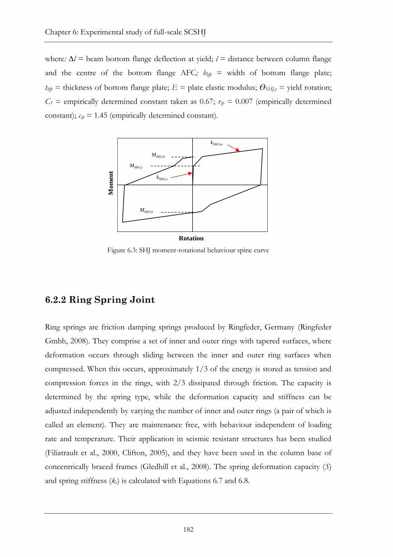
Chapter 6: Experimental study of full-scale SCSHJ
182
where: ∆l = beam bottom flange deflection at yield; l = distance between column flange
and the centre of the bottom flange AFC; bbfp = width of bottom flange plate;
tbfp = thickness of bottom flange plate; E = plate elastic modulus; ӨSHJ,y = yield rotation;
C1 = empirically determined constant taken as 0.67; rsp = 0.007 (empirically determined
constant); csp = 1.45 (empirically determined constant).
Figure 6.3: SHJ moment-rotational behaviour spine curve
6.2.2 Ring Spring Joint
Ring springs are friction damping springs produced by Ringfeder, Germany (Ringfeder
Gmbh, 2008). They comprise a set of inner and outer rings with tapered surfaces, where
deformation occurs through sliding between the inner and outer ring surfaces when
compressed. When this occurs, approximately 1/3 of the energy is stored as tension and
compression forces in the rings, with 2/3 dissipated through friction. The capacity is
determined by the spring type, while the deformation capacity and stiffness can be
adjusted independently by varying the number of inner and outer rings (a pair of which is
called an element). They are maintenance free, with behaviour independent of loading
rate and temperature. Their application in seismic resistant structures has been studied
(Filiatrault et al., 2000, Clifton, 2005), and they have been used in the column base of
concentrically braced frames (Gledhill et al., 2008). The spring deformation capacity (S)
and spring stiffness (ks) is calculated with Equations 6.7 and 6.8.
Mo
men
t
Rotation
MSHJ,0
kSHJ,in
MSHJ,y
MSHJ,0
kSHJ,o

6.2.2 Ring Spring Joint
183
(6.7)
(6.8)
where: ne = number of elements; Se = deformation capacity of one element; F = spring
maximum capacity.
As ring springs are only effective in compression, the configuration shown in Figure
6.4(a) is required for their use in the SCSHJ. The assembly consists of a housing cage
which guides the spring to prevent buckling, and a threaded bar, nuts and endplates to
transfer load from the beams into the column. The ring spring assembly (referred to as
the cartridge) results in a dual-direction acting ring spring similar to that proposed by
Filiatrault et al. (2000). The cartridge is then bolted to the bottom flange of the beam as
shown in Figure 6.1(b). The bar runs through the centre of the spring into the column,
and is held in place by nuts. When a positive moment is applied, the joint remains rigid
till the demand exceeds the pre-compression in the spring. Once this occurs, the column
rotates away from the beam, pulling the bar and opening a gap between endplate A and
the housing cage interface. The ring spring compresses as endplate B is held in position
[Figure 6.4(a)ii]. When a negative moment is applied, the column pushes the bar towards
the beam, opening a gap between endplate B and the housing interface and again, the
spring is compressed [Figure 6.4(a)iii]. The resulting force-displacement behaviour is
shown in Figure 6.4(b), where Fp is the precompression force.
Ring Spring Endplate
NutHousing
(i)
(ii)
(iii)
(a)
B A
Displacement
Force(b)
Fp
ks
Fp1
3
ks1
3
Bar
Figure 6.4: (a) Ring spring cartridge and (b) idealised force-displacement behaviour
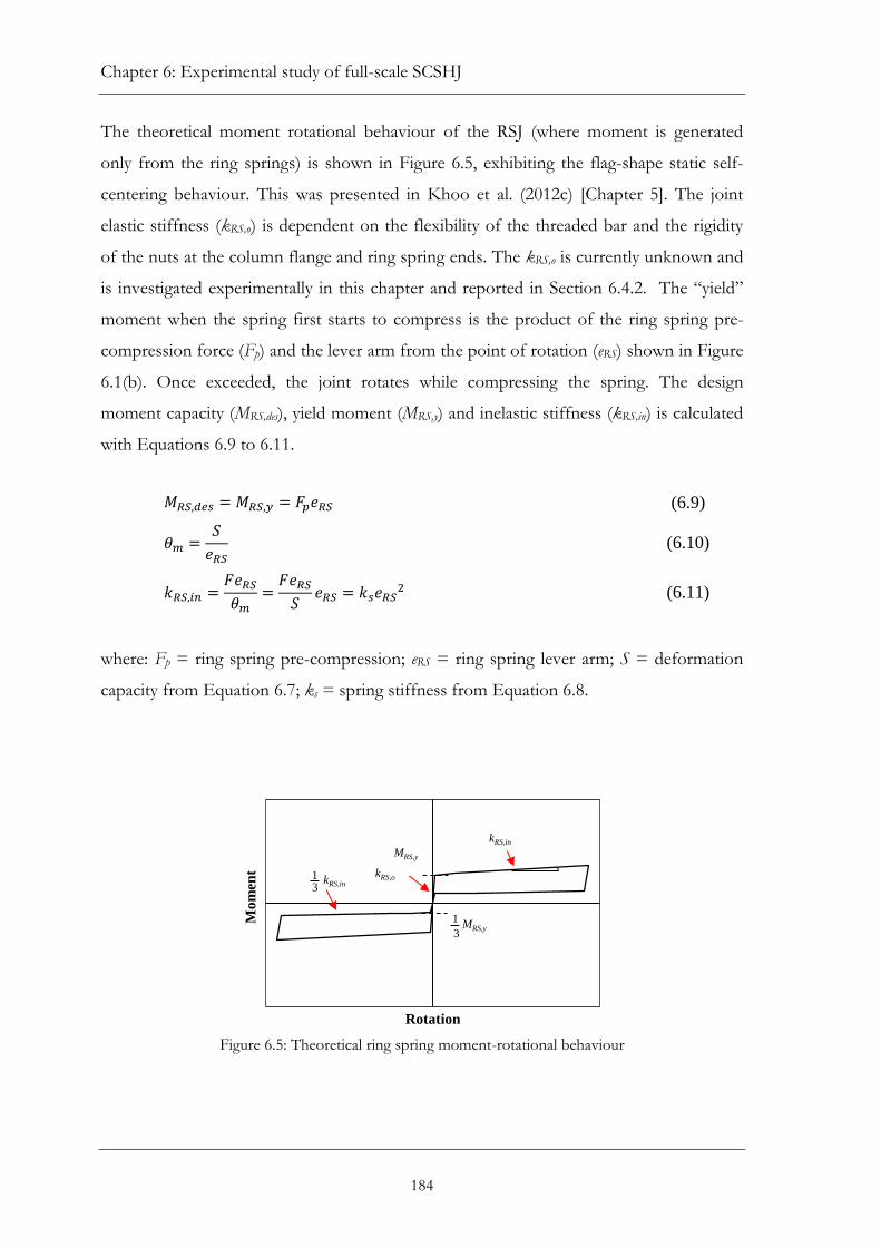
Chapter 6: Experimental study of full-scale SCSHJ
184
The theoretical moment rotational behaviour of the RSJ (where moment is generated
only from the ring springs) is shown in Figure 6.5, exhibiting the flag-shape static self-
centering behaviour. This was presented in Khoo et al. (2012c) [Chapter 5]. The joint
elastic stiffness (kRS,o) is dependent on the flexibility of the threaded bar and the rigidity
of the nuts at the column flange and ring spring ends. The kRS,o is currently unknown and
is investigated experimentally in this chapter and reported in Section 6.4.2. The “yield”
moment when the spring first starts to compress is the product of the ring spring pre-
compression force (Fp) and the lever arm from the point of rotation (eRS) shown in Figure
6.1(b). Once exceeded, the joint rotates while compressing the spring. The design
moment capacity (MRS,des), yield moment (MRS,y) and inelastic stiffness (kRS,in) is calculated
with Equations 6.9 to 6.11.
(6.9)
(6.10)
(6.11)
where: Fp = ring spring pre-compression; eRS = ring spring lever arm; S = deformation
capacity from Equation 6.7; ks = spring stiffness from Equation 6.8.
Figure 6.5: Theoretical ring spring moment-rotational behaviour
Mo
men
t
Rotation
kRS,in
MRS,y
MRS,y1
3
13
kRS,in
kRS,o

6.2.3 Self-centering Sliding Hinge Joint
185
6.2.3 Self-centering Sliding Hinge Joint
The SCSHJ is a combination of the SHJ and RSJ. The SCSHJ remains rigid till the AFC
frictional resistance and ring spring pre-compression (Fp) is exceeded. After which it
rotates as the AFCs slide and the springs compress, with rotational characteristics a
combination of the two components. The flexural behaviour of the SCSHJ can thus be
written as Equation 6.12. The behaviour is illustrated in Figure 6.6, which compares the
SHJ, RSJ and SCSHJ behaviours. This shows improved flag shape curves in the SCSHJ,
which is more pronounced at lower displacements once AFC softening has occurred.
Further details can be found in (Khoo et al., 2012c) [Chapter 5].
There are several benefits compared to the standard SHJ namely: (1) the number of bolts
in the AFC can be reduced, (2) energy stored in the spring contributes to joint re-
centering upon load removal or reversal, and (3) loss in joint elastic strength due to bolt
tension losses in the AFC can be compensated by spring pre-compression. While the RSJ
displays the ideal flag-shaped behaviour, larger springs are required to generate the
required moment capacity which may limit its application due to cost. The SCSHJ
represents a compromise which aims to take advantage of the energy dissipation, sliding
resistance and relatively cheap construction costs of the SHJ, but include benefits of the
ring springs to enhance the recentering ability of the joint during dynamic shake-down of
a structure.
The SCSHJ is designed as a percentage of moment capacity generated by ring springs
(PRS), which is represented by Equation 6.13. This means that a PRS of 0% represents the
standard SHJ where there is only AFC contribution, a PRS of 100% represents the RSJ
where there is only ring spring contribution, and a PRS between 0% and 100% represents
the SCSHJ with both AFC and ring spring contribution. The target PRS is 25% or more to
develop dependable dynamic self-centering behaviour, as indicated by 10-storey frames
studied analytically (Khoo et al., 2012c) [Chapter 5].

Chapter 6: Experimental study of full-scale SCSHJ
186
(6.12)
(6.13)
where: MSCSHJ = SCSHJ moment; MSHJ = moment from AFC (from Equation 6.1);
MRSJ = moment contributed by the ring spring; PRS = percentage of moment capacity
generated by ring springs.
(i)
(ii)
(iii)
Figure 6.6: Idealised moment rotational behaviour (i) SHJ, (ii) RSJ and (iii) SCSHJ (including strength
degradation and load history dependence)
6.3 Subassembly Test Description
6.3.1 Test setup
The test setup (Figure 6.7) simulated an internal connection. The column and beam sizes
were based on the 8th floor of the 10-storey Te Puni Village Tower Building in
Wellington, New Zealand (Gledhill et al., 2008), which is the same frame studied in Khoo
et al. (2012c) [Chapter 5].
The test setup assumed the column mid-height and beam mid-span are points of
inflection. The bottom of the column was pinned to allow rotation and no movement in
the horizontal and vertical direction. The top of the column was free and attached to an
actuator connected to the strong wall. The beam ends were held by a rigid vertical link
with pins at each end to hold the beams vertically and allow rotation and horizontal
movement. The interstorey column height was 3000 mm, while the beams were 2500 mm
long, giving a length L = 5460 mm (shown in Figure 6.7). The column and beams were
Mo
men
t
Rotation
Mo
men
t
Rotation
Mo
men
t
Rotation

6.3.1 Test setup
187
460 UB 74.6 and 360 UB 57 sections respectively, with nominal plastic moments of
498 kNm and 303 kNm. A steel deck concrete slab of 1000 mm width was installed on
the specimen, through the length of the beams. The deck was Comflor 60 (Comflor,
2008) installed perpendicular to the beams and cantilevering 500 mm out each side from
the beam centreline. The slab was 125 mm thick and connected to the beams through six
Ø19 mm shear studs each side (350 mm centres) to prevent sliding between the beams
and deck. The concrete had a 28 day strength f’c of 27.4 MPa. The slab reinforcement was
147/10 (665 equivalent), which is a 300 mm × 300 mm grid with Ø7.5 mm wires of
500 MPa yield strength (Easysteel, 2011). The column was braced at the top to prevent
lateral deflection and twisting, with further bracing to the slab to prevent lateral
deflection of the test specimen.
The joint details are shown in Figure 6.8. All steel plates and sections were Grade 300
steel, except the shims which were abrasion resistant steel with a specified hardness of
370 – 430 HB in the Brinell scale (Bisalloy Steels, 2008). The top flange plates, bottom
flange plates and web plates were welded to the column with fillet welds on both sides.
NorthSouth
h = 3000 mm
Rigid link Rigid link
Actuator
Pin
L = 5460 mm
460 UB 76.6
360 UB 57
125 mm concrete slab
1000
mm
300 x 300 grid, Ø7.5mm,
fy=500 MPa reinforcement
mesh
6 – Ø19 mm shear studs
each side
1.5db
Concrete f’ = 27.4 MPac
Figure 6.7: Test setup

Chapter 6: Experimental study of full-scale SCSHJ
188
All welds were 10 mm E48XX SP fillet welds except the semi-circle stiffener described
below. All bolts were Property Class 8.8 to AS/NZS 1252 (Standards New Zealand,
2006). The beams were bolted to the top flange plates with ten M24 bolts, with Ø26 mm
holes. The top and bottom web bolt groups were each three M16 bolts with Ø18 mm
bolt holes. The AFCs in the bottom flange plate, and bottom web bolt group had 55 mm
long slotted holes to allow sliding. All bolts were proof loaded using the turn of nut
method in accordance with NZS 3404 (Standards New Zealand, 2007).
The column detail was designed to test SHJ, RSJ and SCSHJ connections and therefore
had a unique stiffener configuration to accommodate the ring spring bar through the
middle of the column and transfer load into the web. A semi-circle hole was cut through
the web, with a semi-circular stiffener welded to the column. The semi-circular stiffener
was a Ø168.3 mm outside diameter, 14.27 mm thick tube to ASTM A106B with specified
yield and tensile strengths of 35000 psi (241 MPa) and 60000 psi (414 MPa). It was 190
mm long to extend over the length of the flange. The flange was reinforced with a 168
mm × 190 mm × 20 mm Grade 300 steel plate to prevent yield line failure. This was
welded to the flange and the semi-circular stiffener with a square weld. A Ø38 mm hole
was then drilled through the flange and reinforcing plate. The configuration allowed one
ring spring to be used per joint, which decreased the cost both for experimental purposes
and possibly in practice. While unlike typical SHJ details, the overall joint behaviour and
results are unaffected as the behaviour of the critical components are not compromised.
The column panel zone had a 10 mm thick doubler plate welded to the web, and 12 mm
thick top and bottom continuity plates. Note that there were additional stiffeners
between the top and bottom continuity plates on either side of the column web. This was
because the rig was originally designed for further tests using SMA springs installed
above the bottom flange, on each side of the web, and connected to the column flanges.
The stiffeners were designed to prevent yield line failure of the column flanges. This
series of tests was however not undertaken due to the difficulty of machining nitinol bars.
The nitinol bars failed in brittle fracture when subjected to tensile strains of
approximately 4% during “training”. This was a result of cracks that occurred during the
threading process.

6.3.2 Test details
189
Top flange plate
515 mm × 175 mm × 20 mm
10 – M24 bolts
Web plate
285 mm × 305 mm × 12 mm
Inner web shim
250 × 290 mm × 6 mm
Web cap plate
250 mm × 100 mm × 16 mm
Outer web shim
280 × 100 mm × 6 mm
Bottom flange plate
355 mm × 155 mm × 12 mm
Upper shim
245 mm × 195 mm × 6 mm
Bottom flange cap plate
175 mm × 155 mm × 12 mm
Lower shim
175 mm × 195 mm × 6 mm
Top web bolts
3 – M16
Continuity plates
t =12 mm
Doubler plate
t =10 mm
Column flange stiffener
168 mm × 190 mm × 20 mm
Bottom web AFC bolts
M16
Ø38mm
Semi-circular stiffener
Ø168.3 mm OD, 14.27 mm thick
ASTM A106B
Bottom web AFC bolts
M16
Additional stiffener
t =12 mm
Figure 6.8: Joint components
6.3.2 Test details
The details of the 10 tests are given in Table 6.1, with the ring spring details given in
Table 6.2. The parameters include the number of bottom web bolts, nwbb; number of
bottom flange plate bolts, nbfb; ring spring type; and the number of ring spring elements,
ne. These parameters were chosen to vary the percentage of joint moment capacity
developed by the ring springs (PRS), and the inelastic stiffness developed by the ring
springs (kRS,in). The same beams, column and floor slab were used for all tests. Tests 1
and 2 were standard SHJs, Tests 3 to 7 were SCSHJs with PRS ranging from 20.6% to
52.4%, and Tests 8 and 9 were RSJs. The test numbering is in the order of increasing PRS,
while the order number is the order in which they were undertaken. The loading regime
for each test is shown in Table 6.1 and explained in Section 6.3.3.
Table 6.1 also shows the design moments generated individually by the AFC (MSHJ) and
ring springs (MRSJ), the total design capacity (Mdes) and the dependable moment capacity
(Md). The predicted moment capacities were calculated using Equations 6.1 to 6.13. The
dependable moment capacity Md is defined as Md = MSHJ,0 + MRS,y, and represents the
combined moment resistance contributed by the AFC when both interfaces are sliding,
and the ring spring pre-compression. The ring spring lever arm (eRS) was 446 mm. The
adopted sliding shear capacity (Vss) was 53.8 kN/bolt, which was the average of the
equivalent specimens from the first round of AFC tests (Khoo et al., 2012b) presented in
Chapter 4. This is different from the Vss calculated with the bolt model and was adopted
because the bolts used in the full scale tests were from the same supplier as the first AFC
tests, and would give a better estimate of the actual experimental Vss.

Chapter 6: Experimental study of full-scale SCSHJ
190
The ring springs tested were Type 08000 and Type 12400, with specified maximum force
capacities (F) of 80 kN and 200 kN respectively. The Type 08000 cartridges consisted of
50 elements, giving a theoretical stiffness (ks) = 0.92 kN/mm. The Type 12400 cartridges
consisted of 40 elements, with ks = 1.92 kN/mm. The springs where encased in a steel
housing cage to prevent buckling during compression (Figure 6.9). The cage length was
designed to the spring compressed length (Lp), in order to develop the required level of
pre-compression (Fp). The lengths Lp were 432 mm and 541 mm, corresponding to
theoretical Fp values of 53.5 kN and 113.5 kN for Types 08000 and 12400 respectively.
The details of the ring spring cartridges are summarised in Table 6.2. The cartridges were
tested with a load cell, LVDT and tensioning jack to determine their actual properties.
The ring springs behaved as expected, dissipating energy while maintaining approximately
1/3 of the energy as a restoring force. The two Type 08000 cartridges had Fp of
approximately 53 kN and 50 kN, and ks of 0.89 kN/mm and 0.95 kN/mm. The two
Type 14000 cartridges had Fp of approximately 108 kN and 115 kN, and ks of
1.85 kN/mm and 1.95 kN/mm respectively. These were within 10% of information
provided by the manufacturers. The measured force-displacement curves of these springs
can be found in Figures B-13 and B-14 in Appendix B.
The springs were assembled with the following steps: (1) ring springs with endplates on
each end inserted in the cage through the open end, (2) ring springs compressed with a
jack to a length shorter than the cage, (3) cover plate bolted with four M16 bolts and (4)
compression in the ring spring released. The cartridges were then bolted to the bottom
flange of the beams using four fully tension M16 bolts for each cartridge to prevent
slippage with the beam. The threaded bar was inserted through the ring spring and into
the hole in the column flange. The bar was Grade 8.8 high tensile steel bar of M36
diameter. Four nuts were tightened on either side of the column flange and the ring
spring endplates. The nuts were made from AISI 4140 high tensile steel bar and installed
at snug tight. The assembling and installation of the cartridge was a straightforward
process. This can be completed relatively easily by one person. An example of an
assembled SCSHJ is shown in Figure 6.10.

6.3.2 Test details
191
Table 6.1: Test details – joint design, loading regime and order of tests.
Test no.
nwbb nbfp Ring spring
Design moment (kNm) PRS (%)
Loading Order MSHJ (kNm)
MRS
(kNm) Mdes = My,the
(kNm) Md,the
(kNm)
1 3 4 - 123 0.0 123 178 0.0 SAC 3
2 3 4 - 123 0.0 123 178 0.0 NF 9
3 1 4 Type 08000 92.1 23.9 116 157 20.6 SAC 1
4 0 4 Type 12400 76.6 51.1 128 162 40.0 SAC 4
5 0 4 Type 12400 76.6 51.1 128 162 40.0 SAC_Dy 7
6 0 4 Type 12400 76.6 51.1 128 162 40.0 EQ 8
7 3 0 Type 12400 46.4 51.1 97.5 119 52.4 SAC 6
8 0 0 Type 08000 0.0 23.9 23.9 23.9 100 SAC 2
9 0 0 Type 12400 0.0 51.1 51.1 51.1 100 SAC 5
10 - - - - - - - -
Table 6.2: Details of ring spring cartridges
Ring Spring
Type F (kN) ne Lp
(mm) Pc (%)
Theoretical Measured
Fp (kN)
ks (kN/mm)
Fp (kN)
ks
(kN/mm)
1 8000 83 50 432 64.4 53.5 0.92 53 0.89
2 8000 83 50 432 64.4 53.5 0.92 50 0.95
3 12400 200 40 541 56.7 113.5 1.92 108 1.85
4 12400 200 40 541 56.7 113.5 1.92 115 1.95
Cover platePrestressed ring spring inside
Endplate Nut
Lp Figure 6.9: Ring spring cartridge
Figure 6.10: Assembled SCSHJ

Chapter 6: Experimental study of full-scale SCSHJ
192
6.3.3 Test procedure
Four regimes were used and named as SAC, SAC_Dy, EQ and NF as shown in Figure
6.11. Table 6.1 shows the regimes applied to each test as well as the order that they were
undertaken. SAC [Figure 6.11(a)] is the regime recommended for steel MRF connection
subassembly tests by the SAC Joint Venture (SAC Joint Venture, 2000). This consisted of
symmetric drift cycles of δ = ∆/h, where ∆ = lateral displacements at the top of the
column; h = column height. The regime was six cycles to δ = 0.375%, 0.5%, and 0.75%,
four cycles to δ = 1% and two cycles at δ = 1.5%, 2% and 3% at quasi-static rates of
loading. SAC_Dy is the SAC displacement regime which was modified to dynamic rates
of loading as shown in Figure 6.11(b). This was applied assuming a period of 1.5 s at
δ = 2%, with cycles of different drifts scaled to reflect the same displacement rate at the
top of the column.
The EQ regime [Figure 6.11(c)] is a combination of outputs from time-history analysis
undertaken on the Te Puni Village Tower Building longitudinal frame (Khoo et al.,
2012c) [Chapter 5]. It was the rotational response of an internal connection in the 8th
storey, which the test specimen member sizes were based on. The loading regime was the
response under the maximum considered events of the 1978 Tabas earthquake in Iran,
followed by the 1979 El Centro #6, Imperial Valley earthquake. The latter was scaled to a
target maximum drift of 3%. This was however not achieved due to limitations of the
hydraulic pump, with a maximum drift of 2.44% reached. The NF regime [Figure 6.11(d)]
was adapted from the near-fault loading protocol recommended by the SAC Joint
Venture (2000), which incorporates a large displacement pulse cycle of up to δ = 6%. It
consisted of the recommended regime scaled to a target δ = 4.5%, which corresponded
to the design joint rotation where the bolts hit the end of the slotted hole, followed by
the same recommended regime to a target drift of δ = 6.0%. It was applied at a rate
assuming a period of 6 s at δ = 2%. However, due to the limitations of the hydraulic
pump, the maximum drifts achieved were 4.0% and 5.37% respectively. This is shown in
Figure 6.11(d). All bolts were replaced for each test.

6.4 Results and discussion
193
(a) SAC
(b) SAC_Dy
(c) EQ
(d) NF
Figure 6.11: Load regimes: (a) SAC, (b) SAC_Dy, (c) EQ and (d) NF
6.4 Results and discussion
The experimental results are summarised in Table 6.3. This includes the experimentally
measured yield (My,exp) and dependable (Md,exp) moment capacities, moment at 25 mrad
rotation (M25,exp), ratios between measured and theoretical moment capacities (Mexp/Mthe),
ratio between moment at 25 mrad and dependable moment capacity (M25,exp/Md,exp),
maximum drift (δm), maximum rotation (Өm), residual drift (δr) and final actuator force
(Hf).
The moment capacities Md,exp and M25,exp are the average of the moments in both
directions of drift in the final cycle of loading. For Test 1, Md,exp is the moment as the
joint passes through the zero displacement in the final cycle of loading. For the other
tests, it is the moment at first instance when the curve plateaus past the zero
displacement point in the final cycle of loading. This is because the ring springs have a
zero theoretical force at the plumb position. The Mexp/Mthe ratios compare the results
-4
-2
0
2
4
Dri
ft δ
(%)
Time
h
δ = ∆/h∆
-4
-2
0
2
4
0 5 10 15 20 25
Dri
ft δ
(%)
Time (s)
-3
-2
-1
0
1
2
3
0 20 40 60 80 100
Dri
ft (
%)
Time (s)
-6
-4
-2
0
2
4
6
0 5 10 15 20 25 30 35
Dri
ft (
%)
Time (s)
Break

Chapter 6: Experimental study of full-scale SCSHJ
194
with the rotational models, while M25,exp/Md,exp gives an indication of post-yield joint
stiffness and joint overstrength. The joint rotations (Ө) were determined through
measuring the displacement of the beam bottom flange relative to the column face (∆bfp).
The point of rotation was assumed to be the middle of the top flange plate to column
interface. This gave a Ө = ∆bfp/(db+ 0.5ttfp), where db = beam depth; ttfp = top flange plate
thickness. The results presented are the average of north and south side joints at any
time.
The residual drift (δr) is the column drift when the load is slowly reduced to zero from
the maximum drift of approximately δ = 3.0%. The load Hf is the final actuator load
when the column is brought back to the vertical plumb position at the end of the load
regime. Both δr and Hf give an indication of the recentering ability of the joints, but do
not take dynamic effects into account. The closer they are to zero, the better the joint
recentering properties.
As the SHJ and RSJ involve only the contribution of the AFC and ring springs
respectively, they serve as the baseline to which the SCSHJ tests can be compared, in
which these contributions are combined. The behaviour of the standard SHJ and RSJs
are therefore discussed first, followed by the SCSHJ. This would then be followed by a
description of the test results from the dynamic and near fault type load regimes, a
discussion on secondary element effects, and the damage to the floor slab.
Table 6.3: Test results
Test no. My,exp
(kNm) Md,exp
(kNm) M25,exp
(kNm) My,exp/ My,the
Md,exp/ Md,the
M25,exp/ Md,exp
δm (%)
Ɵm (mrad)
δrb
(%) Hf
(kN)
1 130 168 254 1.06 0.94 1.51 3.04 26.1 -2.0 74.4
2 115 138 175 0.93 0.78 1.27 5.37 43.7 - -
3 138 165 243 1.19 1.05 1.47 3.03 28.2 -1.9 58.0
4 130 158 257 (221a) 1.02 0.97 1.63 3.03 26.7 -1.51 53.6
5 121 165 244 (226a) 0.95 1.01 1.48 2.87 25.3 -1.48 58.4
6 129 170 220a 1.01 1.04 1.29a 2.44 20.0 - 3.0
7 75.0 110 170 0.77 0.92 1.55 3.07 31.9 -1.14 16.1
8 29.8 29.8 60.0 1.25 1.25 2.01 3.12 32.0 -0.02 0.4
9 64.4 64.4 125 1.26 1.26 1.94 3.09 30.2 0.36 -8.4
10 - 6 30.5 - - 5.08 3.60 35.5 - - a Moment at 20 mrad (M20,exp)
b Negative values indicate drift in the south direction
6.4.1 Sliding Hinge Joint behaviour
195
6.4.1 Sliding Hinge Joint behaviour
Test 1 was the standard SHJ tested with the SAC loading regime. The load-drift
relationship (H-δ) and joint moment-rotation (M-Ө) are presented in Figure 6.12(a) and
(c). The behaviour was comparable to SHJ tests undertaken by Clifton (2005) and
MacRae et al. (2010). It behaved similar to a rigid connection under elastic loading, with
stiffness comparable to rigid connections. This is shown in the near identical hysteresis
behaviour for all elastic cycles up to approximately 0.47% drift when sliding first
commenced. The yield moment (My,exp) was 130 kNm, which is slightly higher than the
theoretical My,the of 123 kNm. This gave a My,exp/ My,the ratio of 1.06 as shown in Table 6.3.
At the onset of inelastic rotation, the AFC resistance quickly built up as the second
surface started to slide. It however did not exhibit the theoretical two stage increase seen
in component tests of the AFC, which is due to the bolts rotating and smearing the
double slip effect (MacRae et al., 2010). The resistance then plateaued as the AFC
reached the stable sliding state of both surfaces. There was still a reasonably large
inelastic stiffness at this stage which further increased the moment resistance. At load
reversal, the resistance was near zero, which then built up as it was pushed in the other
direction, with the two stage increase in friction again smeared out.
The joint stiffness is dependent on the maximum rotation previously reached. At the first
cycle of each increase in rotation, the inelastic stiffness was the same as the previous cycle
(which was to a lower demand). However in subsequent cycles to the same rotation, the
stiffness then dropped and stabilised with further cycles. This could be due to the
influence of the floor slab, which increases the joint strength and stiffness, but undergoes
damage, which then reduces its contribution in subsequent cycles of loading. The results
nevertheless showed that the SHJ produced repeatable and near identical curves for
cycles to the same level of deformation once it stabilised. In the final cycle of loading, the
dependable moment capacity while passing through the zero displacement Md,exp was
168 kNm [Figure 6.12(c)], which was within 10% of the predicted Md,the of 178 kNm
(Table 6.1), giving a Md,exp/Md,the ratio of 0.94. The M25,exp was 254 kNm, giving a

Chapter 6: Experimental study of full-scale SCSHJ
196
M25,exp/Md,exp ratio of 1.51, indicating the large inelastic stiffness due to secondary element
effects as described in Section 6.2.1.
The column residual drift δr was approximately 2.0%, when the load was slowly released
from the maximum drift. When the column was forced back to its plumb position, the
final actuator load was Hf = 74.4 kN [shown in Figure 6.12(a) and Table 6.3]. These
results show that the SHJ does not display static self-centering behaviour. As mentioned
above, this does not take dynamic effects into account, but provides a simple method of
comparing the self-centering abilities of the joints studied.
6.4.2 Ring Spring Joint behaviour
Tests 8 and 9 represented RSJs with PRS = 100%, and were tested with the SAC loading
regime. The load-drift (H-δ) and joint moment-rotation (M-Ɵr) response of Test 9 is
presented in Figure 6.12(b) and (d).
The elastic stiffness (kRS,o) was much lower than that of the SHJ, with measured
stiffnesses of 13.9 kNm/mrad and 21.5 kNm/mrad for Tests 8 and 9 respectively. Both
displayed definite yield moments (My,exp) indicating the point where the pre-compression
(Fp) was exceeded and the ring springs started to compress. This occurred at
approximately 0.8 mm and 1.1 mm deflections of the bottom beam flange relative to the
column face, corresponding to rotations of approximately 2.2 mrad and 3.0 mrad. The
My,exp values were 29.8 kNm and 64.4 kNm (Table 6.3) for Tests 8 and 9. These were
higher than the predicted My,the values of 23.9 kNm and 51.1 kNm (Table 6.1), giving
My,exp/My,the ratios of 1.25 and 1.26 respectively.

6.4.2 Ring Spring Joint behaviour
197
(a) Test 1 – load drift response
(b) Test 9 – load drift response
(c) Test 1 – moment rotational response
(d) Test 9 – moment rotational response
Figure 6.12: Cyclic response of Test 1 (SHJ) and Test 9 (RSJ): (a) Test 1 load-drift, (b) Test 9 load-
drift, (c) Test 1 joint moment-rotation and (d) Test 9 joint moment-rotation
The low elastic stiffness was due to the lack of pretension in the threaded bar connecting
the cartridges and the column flanges, causing the elastic stiffness to be dependent on the
flexibility of the bar and nuts. While the bar diameter was sufficient to prevent buckling,
it had considerable flexibility and deformation in the threads when loaded axially. A slight
bending action was visually observed under compression in negative joint rotation. As
the same bar and nuts were used for both tests, it was expected that the elastic stiffness
would be the same for both tests. This was however not the case due to the variability in
snug tight installation of the bolts.
Once in the inelastic range, the ring spring cartridges performed as expected,
compressing the springs in both positive and negative joint rotations. This gave constant
inelastic stiffness (kin,exp) in both directions of loading up to a rotation of approximately
20 mrad. The kin,exp was approximately 1.0 kNm/mrad and 2.0 kNm/mrad compared to
kin,the of 0.2 kNm/rad and 0.4 kNm/mrad calculated with Equation 6.11 for Tests 8 and 9
-200
-100
0
100
200
-4 -3 -2 -1 0 1 2 3 4
Lo
ad
(k
N)
Drift δ (%)
H (positive)δ
f
δr
H
Regime = SAC
PRS = 100%
-200
-100
0
100
200
-4 -3 -2 -1 0 1 2 3 4
Lo
ad
(k
N)
Drift δ (%)
H
H (positive)δ
f
δr
Regime = SAC
PRS = 0%
-300
-200
-100
0
100
200
300
-35 -30 -25 -20 -15 -10 -5 0 5 10 15 20 25 30 35
Mo
men
t (k
Nm
)
Rotation (mrad)
M25,des
M d,exp
M25,des
Regime = SAC
PRS = 100%Md,exp
-300
-200
-100
0
100
200
300
-35 -30 -25 -20 -15 -10 -5 0 5 10 15 20 25 30 35
Mo
men
t (k
Nm
)
Rotation (mrad)
M d,exp
Md,exp
M
M
25,exp
25,exp
1/5M y,the
Regime = SAC
PRS = 0%

Chapter 6: Experimental study of full-scale SCSHJ
198
respectively. This resulted in kin,exp/kin,the ratios of approximately 5 for both tests, and high
M25,exp/Md,exp ratios of 2.01 and 1.94. Above 25 mrad, the stiffness increased sharply,
developing maximum moments of 129 kNm and 176 kNm at maximum rotation, which
was much higher than the M25,exp of 60 kNm and 125 kNm. While the secondary element
effects were more significant compared to Test 1 (SHJ), this may be due to the larger
rotations that Tests 8 and 9 were subjected to. As a result of these large increases in
moment, Test 10 was undertaken to investigate the extent of secondary element
contribution. This is covered in Section 6.4.6.
Upon load reversal or removal, the RSJs displayed the ideal flag-shape, static recentering
curve, with the load almost zero as the column passed through the plumb position. The
self-centering ability of the joint is clearly shown by the residual drift δr and final actuator
load Hf. The δr was -0.02% and -0.36% from the maximum drift, and the Hf was 0.4 kN
and 8.4 kN for Tests 8 and 9 respectively. The RSJ also provided good energy dissipation
as seen in the hysteretic behaviour. The restoring force was however approximately 1/5
of the calculated force, rather than 1/3, as shown in Figure 6.12(d). The RSJ displayed
the characteristics of the ring springs, and developed stable, ideal flag-shaped self-
centering hysteretic behaviours. However, the RSJ model presented in Section 6.2.2
underestimated the moment resistance and rotational stiffness of the RSJs as shown in
the Mexp/Mthe ratios.
The ring springs had high deflection capabilities, which is a product of designing the
springs with low stiffness to reduce the “post-yield” joint stiffness and therefore
overstrength demands. The ring spring components can therefore be designed to
theoretically undergo unlimited levels of rotation till failure is governed by structure
collapse due to instability under extreme drifts. However, a failure mechanism as a result
of buckling of the bars under negative rotation due to bending may also occur. The
maximum rotation Өm that any connection with ring springs (either RSJ or SCSHJ) was
subjected to was Test 8, which was tested to 32 mrad. As the connections were not tested
to failure or to higher levels of rotations, there are no experimental results to determine if
this would occur. It is therefore recommended that the failure mechanism of connections
with the proposed ring spring configuration is investigated experimentally in the future.

6.4.3 Self-centering Sliding Hinge Joint behaviour
199
6.4.3 Self-centering Sliding Hinge Joint behaviour
Tests 3, 4 and 7 were designed with PRS of 20.6%, 40.0% and 52.4% respectively. Their
M-Ө behaviour displayed a combination of the SHJ and RSJ characteristics, and is shown
in Figure 6.13(a)-(c). The SCSHJ tests behaved as rigid connections under elastic loading,
until yield occurred at drifts of approximately 0.56%, 0.45% and 0.33% respectively. The
yield moments (My,exp) were 138 kNm, 130 kNm and 75 kNm for Tests 3, 4 and 7
respectively, compared to the predicted values of 116 kNm, 128 kNm and 97.5 kNm
shown in Table 6.1. This gave My,exp/My,the ratios of 1.19, 1.02 and 0.77. The decrease in
ratio showed that the yield moment decreased with increasing PRS, which was expected
given the lower elastic stiffness provided by the cartridges. This indicated that sliding in
the AFC commenced before the cartridges started to compress. Once the latter were
engaged, the rotational stiffness was a combination of the two contributing resistances.
The SCSHJs tests showed that the hysteresis curves better resembled the self-centering
flag shaped curves of the RSJs as the PRS increased. This is shown in the M-Ө curves of
Tests 1, 4 and 9 shown in Figure 6.13(d), where the moments were normalised with their
experimental dependable moment capacity (Md,exp) in Table 6.3. The improved self-
centering ability of the joints is also shown by the reduced residual drifts (δr). The SHJ
had a δr of 2.0% (Test 1), which decreased to 1.9%, 1.51% and 1.14% in Tests 3, 4 and 7.
It was nevertheless higher than the δr of 0.02% and 0.36% in the RSJs (Tests 8 and 9).
Likewise, the final actuator load (Hf) decreased with increasing PRS. From the maximum
drift, Hf was 74.4 kN in the SHJ (Test 1), but decreased to 58 kN, 53.6 kN and 16.1 kN
in Tests 3, 4 and 7. The SCSHJs were again higher than the Hf of 0.4 kN and 8.4 kN in
the RSJs (Tests 8 and 9). The maximum PRS of 52.3% was insufficient to develop full
static recentering curves. In order to achieve static recentering, a larger PRS is required
which would increase the cost of the system and may limit its implementation. However,
a structure would in reality be subjected to dynamic and shake-down effects, which
would reduce residual drifts. This effect has been studied analytically (Khoo et al., 2012c)
[Chapter 5] and could be studied experimentally through shake-table tests.

Chapter 6: Experimental study of full-scale SCSHJ
200
6.4.4 Loading rate effects
The joints in Tests 5 and 6 were identical to the joint in Test 4, and designed with a
PRS = 40%. Test 5 was undertaken with the SAC_Dy regime, which brought the
specimen to approximately the same displacements as the quasi-static SAC regime
applied to Test 4, but at dynamic rates of loading. This was undertaken to determine any
loading rate effects in the SHJ. Their M-Ө curves are compared in Figure 6.13(e),
showing near identical behaviour. The moment capacities My,exp, Md,exp and M25,exp were
121 kNm, 165 kNm and 244 kNm in Test 5, which were within 10% of the 130 kNm,
158 kNm and 257 kNm in Test 4. The self-centering responses were also similar, with
δr = 1.48% and Hf = 58.4 kN in Test 5 compared to δr = 1.48% and Hf = 53.6 kN for
Test 4. These values are given in Table 6.3. Test 6 [Figure 6.13(f)] was loaded with the
EQ regime in Figure 6.11(c). The experimental My,exp and Md,exp values were 129 kNm and
170 kNm, which was within 10% of both Tests 4 and 5. Test 6 was subjected to a
maximum rotation of approximately 20 mrad, generating a maximum moment (M20,exp) of
220 kNm. This is was also similar to the equivalent M20,exp of Tests 4 and 5, which were
221 kNm and 226 kNm respectively (Table 6.3). This indicates there is no significant
difference between the static and dynamic response of the joints.
6.4.5 Near fault type action performance
Test 2 was undertaken with the NF regime shown in Figure 6.11(d), testing the specimen
to a maximum drift of 5.37%. The M-Ө curve is shown in Figure 6.13(g). The joint
capacities at various stages of loading were lower than Test 1 (identical SHJ), with My,exp,
Md,exp and M25,exp of 115 kNm, 138.0 kNm and 174.9 kNm compared to 130 kNm, 167.8
kNm and 254.4 kNm in Test 1. The Md,exp for Test 2 was taken as the moment at the
final cycle as it passed through the zero position, with M25,exp taken as the moment at 25
mrad of that same cycle. These values are summarised in Table 6.3, and represent an
average drop in capacity of approximately 20%. The extreme deformations in the NF
regime caused the bolts to hit the end of the slotted hole, which is seen as the spike in the
positive rotation. This resulted in further bolt inelastic deformation and tension loss.

6.4.6 Secondary element effects
201
6.4.6 Secondary element effects
The joint inelastic stiffnesses were significant as shown by M25,exp/Md,exp ratios ranging
from 1.27 to 2.01. This is due to secondary element effects, which include floor slab
contribution, prying of the flange plates and additional resistance from the web plate
bolts. The overlaying concrete slab increases the joint strength and stiffness, but sustains
damage as it undergoes cyclic loading, causing variability in joint strength and stiffness
between cycles. The damage is described in more detail in Section 6.4.7. The web plate
bolts are also contributing factors due to the rotational behaviour of the web plate about
the beam, causing a vertical component of motion, in contrast to the longitudinal
direction motion of the bottom flange plate. This adds additional demand on the top web
bolts (designed to carry joint vertical shear) and increases moment resistance. This is also
the case for the bottom web AFC, where impact marks on the bolts and slotted hole
indicate vertical displacement during joint rotation.
Test 10 was therefore undertaken to investigate the extent of secondary element
contribution, and effect on joint overstrength. The bolts in the AFC were left loose, and
the ring spring cartridges were removed, giving negligible design moment capacity. It was
tested with the SAC regime, with the M-Ө curve shown in Figure 6.13(h). The resistance
was under 6 kNm up to 15 mrad, before it increased to 30.5 kNm at 25 mrad (values
shown in Table 6.3). There was then a significant spike which resulted in maximum
moment of 88 kNm at the maximum rotation of 35.5 mrad. At larger drifts, the bolts
would hit the end of the slotted holes and significantly increase the force again. As the
expected operation of the SHJ is within 25 mrad, corresponding to 3% drift, these effects
are expected to be limited under the DLE.
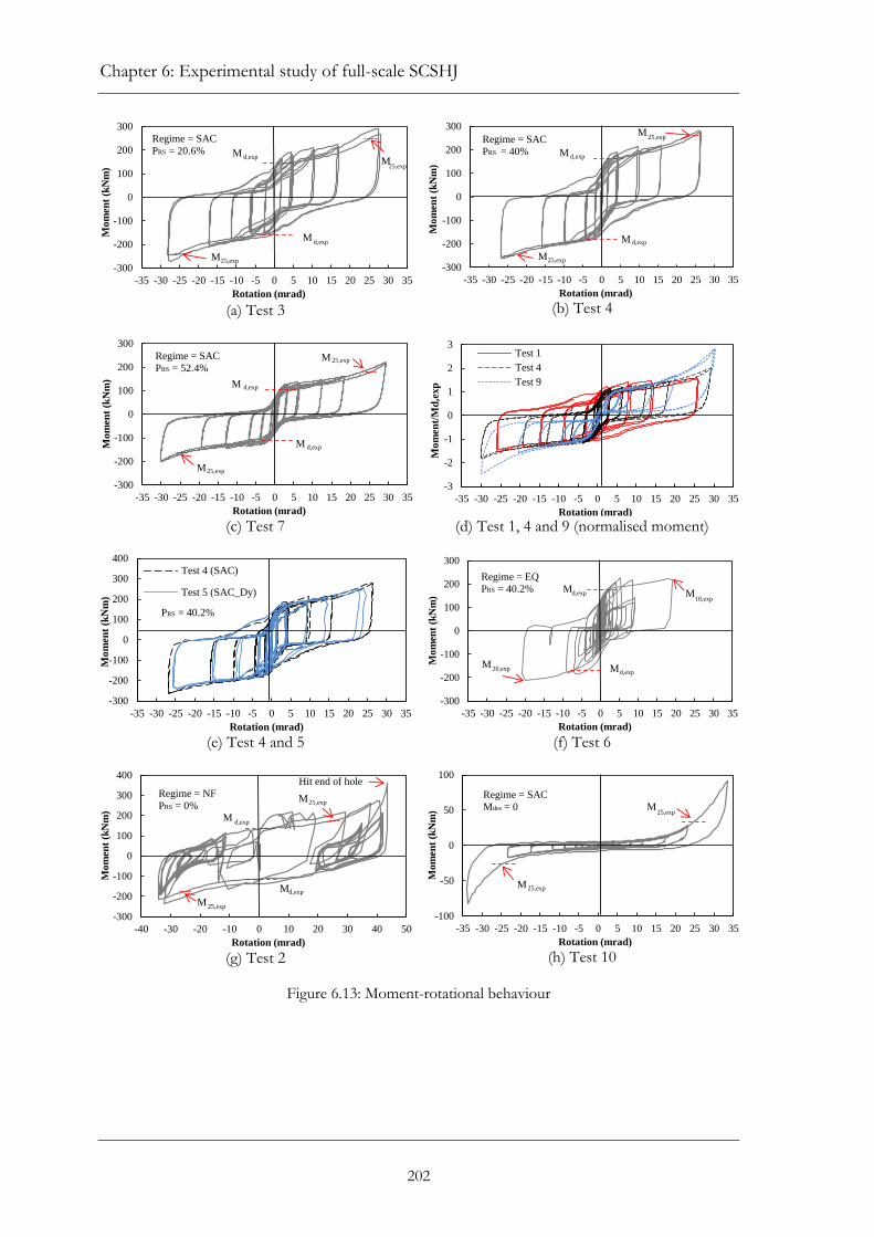
Chapter 6: Experimental study of full-scale SCSHJ
202
(a) Test 3
(b) Test 4
(c) Test 7
(d) Test 1, 4 and 9 (normalised moment)
(e) Test 4 and 5
(f) Test 6
(g) Test 2
(h) Test 10
Figure 6.13: Moment-rotational behaviour
-300
-200
-100
0
100
200
300
-35 -30 -25 -20 -15 -10 -5 0 5 10 15 20 25 30 35
Mo
men
t (k
Nm
)
Rotation (mrad)
M d,exp
d,expM
M
M25,exp
25,exp
Regime = SAC
PRS = 20.6%
-300
-200
-100
0
100
200
300
-35 -30 -25 -20 -15 -10 -5 0 5 10 15 20 25 30 35
Mo
men
t (k
Nm
)
Rotation (mrad)
M d,exp
d,expM
M
M25,exp
25,exp
Regime = SAC
PRS = 40%
-300
-200
-100
0
100
200
300
-35 -30 -25 -20 -15 -10 -5 0 5 10 15 20 25 30 35
Mo
men
t (k
Nm
)
Rotation (mrad)
M d,exp
d,expM
M
M25,exp
25,exp
Regime = SAC
PRS = 52.4%
-3
-2
-1
0
1
2
3
-35 -30 -25 -20 -15 -10 -5 0 5 10 15 20 25 30 35
Mo
men
t/M
d,e
xp
Rotation (mrad)
Test 1
Test 4
Test 9
-300
-200
-100
0
100
200
300
400
-35 -30 -25 -20 -15 -10 -5 0 5 10 15 20 25 30 35
Mo
men
t (k
Nm
)
Rotation (mrad)
Test 4 (SAC)
Test 5 (SAC_Dy)
PRS = 40.2%
-300
-200
-100
0
100
200
300
-35 -30 -25 -20 -15 -10 -5 0 5 10 15 20 25 30 35
Mo
men
t (k
Nm
)
Rotation (mrad)
Md,exp
d,expMM
M18,exp
20,exp
Regime = EQ
PRS = 40.2%
-300
-200
-100
0
100
200
300
400
-40 -30 -20 -10 0 10 20 30 40 50
Mo
men
t (k
Nm
)
Rotation (mrad)
Md,exp
d,expM
M
M25,exp
25,exp
Regime = NF
PRS = 0%
Hit end of hole
-100
-50
0
50
100
-35 -30 -25 -20 -15 -10 -5 0 5 10 15 20 25 30 35
Mo
men
t (k
Nm
)
Rotation (mrad)
M
M25,exp
25,exp
Regime = SAC
Mdes = 0

6.4.7 Slab damage
203
6.4.7 Slab damage
The response of the earliest test (Test 3) is presented, which best describes the expected
damage under a severe earthquake shaking. The cracks in the floor slab at various levels
of drift are illustrated in Figure 6.14(a). A hairline crack first developed at the column
flange interface at δ = 0.5%. Further cracks developed parallel to and away from the
column flange as the drift demand increased. Above 1.5% and 2.0%, cracks occurred
perpendicular to the column flange as a result of the concrete bearing on the shear studs.
The crack at each side of the column face eventually opened to around 1-2 mm during
positive rotation [eg. Figure 6.14(b)], and there was minor crushing of the concrete
around the column flanges at approximately 3.0% drift [Figure 6.14(c)]. All other cracks
remain hairline.
The level of slab damage is consistent with the stable and repeatable hysteretic behaviour,
as the rotation about the top flange plate reduced floor slab demands and interaction
with the joint behaviour. There was little change to the cracks away from the column in
subsequent tests. While damage accumulated around the column with further crushing of
the concrete, it was minimal and easily repairable. The extent of damage after Test 6 is
shown in Figure 6.14(d). This was the final condition of the slab around the concrete
after it was tested to 24 cycles of δ greater than 2%, which is well beyond the demand
expected during a major earthquake.

Chapter 6: Experimental study of full-scale SCSHJ
204
(a) Crack pattern after Test 3
(b) Crack at 3% drift (Test 6)
(c) Concrete crushing after Test 3
(d) Damage after Test 6
Figure 6.14: Slab damage
6.5 SCSHJ model
The experimentally measured values of Test 1 were within 10% of the predicted values,
showing the adequacy of the SHJ model previously developed (Clifton, 2005, Pantke,
2001). This is also illustrated in Figure 6.15(a), which compares the experimental results
with the model in RUAUMOKO (Carr, 2007). The comparisons were based on predicted
moment capacities calculated using the Vss from the first round of AFC tests, which is
higher than the expected average capacity as computed by the bolt model in Chapter 4.
This was the most reliable estimate of the actual experimental Vss available, and gives an
indication of the accuracy of the SHJ model. The average moment capacities of SHJs in
practice is expected to be similar to that calculated from the bolt model Vss, with similar
variations as the AFCs, due to bolt strength and coefficient variability as described in
Chapter 4.

6.5 SCSHJ model
205
The RSJ model presented in Section 6.2.2 significantly underestimated the moment
capacity of the joint. It is therefore necessary to modify the model based on the
experimental results. It was not possible to model the elastic stiffness given the variability
in the threaded bar and bolts as described in Section 6.4.2. It would however be in the
order of 1 mm deflection at the beam end to column face under similar configurations,
with the elastic stiffness calculated with Equations 6.14 and 6.15. It should be noted that
this is an approximation, with further experimental testing and/or modelling required to
more accurately model the elastic stiffness. In the inelastic state, the behaviour (described
in Section 6.4.2) can be summarised as (1) the yield moment was 1.25 times higher than
the theoretical moment, (2) the rotational stiffness was 5 times higher than the
theoretically values, and (3) the recentering force was 1/5 of the theoretical pre-
compression. Equations 6.9 and 6.11 are therefore modified to Equations 6.16 and 6.17.
Figure 6.15(b) shows the revised model compared to the experimental results of Test 9
(RSJ), showing a reasonable fit to a rotation of 20 mrad. As previously mentioned, the
enhancement in strength and stiffness is a function of the overall subassemblage
behaviour. Because of the number of potential sources of this extra strength and stiffness
it is not possible to establish a meaningful determination of the extra capacity by first
principles. While these effects are expected to be similar for similarly proportioned joints
to a range of beam sizes and joint capacities, the model should be verified with further
experimental studies on connections of difference sizes.
(6.14)
(6.15)
(6.16)
(6.17)
where: ӨRS,y = yield rotation (rad), db = beam depth (mm); ttfp = top flange plate
thickness (mm); MRS,y = yield moment (kNm); kRS,o = elastic stiffness (kNm/rad);
MRS,y,mod = modified model yield moment; kRS,in,mod = modified model inelastic stiffness;
cy = constant adopted as 1.25; ck = constant adopted as 5.

Chapter 6: Experimental study of full-scale SCSHJ
206
(a) Test 1 (b) Test 9
Figure 6.15: Comparison between model and experimental results
6.6 Summary and conclusions
1. The SHJ behaved like a rigid connection till sliding commenced when
the frictional resistance was exceeded. It then produced stable and
repeatable hysteretic behaviour but not self-centering properties.
2. The RSJs produce stable and repeatable hysteretic behaviour,
displaying ideal flag-shaped self-centering curves. The dual-directional
acting ring spring behaved as expected, compressing under both
positive and negative joint rotations. Further research is recommended
to experimentally investigate the possible failure mechanism of the ring
spring bar buckling under joint negative rotation.
3. The SCSHJ displayed a combination of the SHJ and RSJ behaviours.
As the PRS increased, the joint better resembled the flag-shaped curves
of the RSJs which improved recentering. The PRS tested was
insufficient to develop static recentering properties.
4. Tests undertaken at seismic-dynamic rates of loading showed negligible
difference in behaviour compared to quasi-static tests.
5. The SHJ had an average of 20% drop in capacity under a near fault
type pulse action. The bolts hit the end of the slotted hole under
extreme deformations, causing a spike in moment resistance.
6. Secondary elements, such as the slab contribution, prying of flange
plates and web bolts increase joint strength and stiffness. This
becomes significant above 25 mrad, causing a spike in the moment
-300
-200
-100
0
100
200
300
-30 -25 -20 -15 -10 -5 0 5 10 15 20 25 30
Mo
men
t (k
Nm
)
Rotation (mrad)
Experimental
Model
-200
-150
-100
-50
0
50
100
150
200
250
-35-30-25-20-15-10 -5 0 5 10 15 20 25 30 35
Mo
men
t (k
Nm
)
Rotation (mrad)
Experimental
Model

6.7 References
207
7. resistance. At larger drifts, the bolt would reach the end of the slotted
hole and significantly increasing the force again. There was minimal
crushing at the column/slab interface which is easily repaired, with
further hairline cracking away from the column, showing the
effectiveness of the joint in minimising floor slab damage.
8. The model previously developed for the SHJ gives good representation
of the joint behaviour, with experimentally measured values within
10% of predictions. The RSJ had enhanced moment resistance and
rotational stiffness, which led to modification to the theoretical model
with experimentally determined parameters. As the modified RSJ
model is based on just one test, it should be verified with further
testing of connections of difference sizes. Further studies are also
required to more accurately model the RSJ elastic stiffness.
6.7 References
Bisalloy Steels (2008). Bisplate Technical Guide. Unanderra, Australia.
Carr, A. (2007). RUAUMOKO 2D. Civil Engineering Department, University of
Canterbury, Christchurch, New Zealand.
Chou, C.-C. and Chen, J.-H. (2011). "Development of floor slab for steel post-tensioned
self-centering moment frames." Journal of Constructional Steel Research, 67(10): 1621-
1635.
Chou, C.-C., Wang, Y.-C. and Chen, J.-H. (2008). "Seismic design and behavior of post-
tensioned steel connections including effects of a composite slab." Engineering
Structures, 30(11): 3014-3023.
Christopoulos, C., Filiatrault, A., Uang, C.-M. and Folz, B. (2002). "Posttensioned energy
dissipating connections for moment-resisting steel frames." Journal of Structural
Engineering, 128(9): 1111-1120.

Chapter 6: Experimental study of full-scale SCSHJ
208
Clifton, G. C. (2005). “Semi-rigid joints for moment-resisting steel framed seismic-
resisting systems.” Department of Civil and Environmental Engineering,
University of Auckland, Auckland.
Comflor. (2008). Comflor 60 Composite Floor Decking. Auckland, New Zealand.
Danner, M. and Clifton, C. (1995). “Development of moment-resisting steel frames
incorporating semi-rigid elastic joints.” Report R4-87. Heavy Engineering
Research Association (HERA), Manukau City, New Zealand.
DesRoches, R., Taftali, B. and Ellingwood, B. R. (2010). "Seismic performance
assessment of steel frames with shape memory alloy connections. Part I - Analysis
and seismic demands." Journal of Earthquake Engineering, 14(4): 471-486.
Easysteel, F. (2011). The Steel Book.
Ellingwood, B. R., Taftali, B. and DesRoches, R. (2010). "Seismic performance
assessment of steel frames with shape memory alloy connections. Part II -
Probabilistic seismic demand assessment." Journal of Earthquake Engineering, 14(5):
631-645.
Filiatrault, A., Tremblay, R. and Kar, R. (2000). "Performance evaluation of friction
spring seismic damper." Journal of Structural Engineering, 126(4): 491-499.
Garlock, M. and Li, J. (2008). "Steel self-centering moment frames with collector beam
floor diaphragms." Journal of Constructional Steel Research, 64(5): 526-538.
Garlock, M., Ricles, J. M. and Sause, R. (2005). "Experimental studies of full-scale
posttensioned steel connections." Journal of Structural Engineering, 131(3): 438-448.
Gledhill, S. M., Sidwell, G. K. and Bell, D. K. (2008). “The damage avoidance design of
tall steel frame buildings - Fairlie Terrace Student Accommodation Project

6.7 References
209
Victoria University of Wellington.” 2008 NZSEE Conference, Taupo, New Zealand.
Iyama, J., Seo, C. Y., Ricles, J. M. and Sause, R. (2009). "Self-centering MRFs with
bottom flange friction devices under earthquake loading." Journal of Constructional
Steel Research, 65(2): 314-325.
Khoo, H. H., Clifton, C., Butterworth, J. W., MacRae, G. A. and Ferguson, G. (2012a).
"Influence of steel shim hardness on the Sliding Hinge Joint performance." Journal
of Constructional Steel Research, 72(0): 119-129. [Chapter 3]
Khoo, H. H., Clifton, G. C., Butterworth, J. W. and MacRae, G. A. (2012b). “Shim and
bolt size effects on the Asymmetric Friction Connection.” 7th STESSA Conference
on the Behaviour of Steel Structures in Seismic Areas. Santiago, Chile.
Khoo, H. H., Clifton, C., Butterworth, J. W., MacRae, G. A., Gledhill, S. and Sidwell, G.
(2012c). “Development of the self-centering Sliding Hinge Joint with friction ring
springs.” Journal of Constructional Steel Research, 78(2012): 201-211. [Chapter 5]
Kim, H.-J. and Christopoulos, C. (2008). "Friction damped posttensioned self-centering
steel moment-resisting frames." Journal of Structural Engineering, 134(11): 1768-1779.
King, A. (2007). “Design of collector elements for self-centering moment resisting
frames.” Master of Science in Civil Engineering, Purdue University.
MacRae, G. A., Clifton, C., MacKinven, H., Mago, N., Butterworth, J. and Pampanin, S.
(2010)."The Sliding Hinge Joint moment connection." Bulletin of the New Zealand
Society for Earthquake Engineering, 43(3): 202-212.
Ocel, J., DesRoches, R., Leon, R. T., Hess, W. G., Krumme, R., Hayes, J. R. and
Sweeney, S. (2004). "Steel beam-column connections using shape memory alloys."
Journal of Structural Engineering, 130(5): 732-740.

Chapter 6: Experimental study of full-scale SCSHJ
210
Pantke, M. (2001). “Development of analytical models for SHJ and SHJS.” Report for 2nd
Industrial Internship, Heavy Engineering Research Association, Manukau City,
New Zealand.
Priestley, M. J. N. and MacRae G. A. (1996). "Seismic tests of precast beam-to-column
joint subassemblages with unbonded tendons." PCI Journal, 41(1): 64-80.
Ricles, J. M., Sause, R., Garlock M. and Zhao, C. (2001). "Post-tensioned seismic-
resistant connections for steel frames." Journal of Structural Engineering, 127(2): 113-
121.
Ringfeder Gmbh (2008). Damping Technology. Catalogue R60. Krefeld, Germany.
Roeder, C. W. (2002). "Connection performance for seismic design of steel moment
Frames." Journal of Structural Engineering, 128(4): 517-525.
SAC Joint Venture (2000). “Loading histories for seismic performance testing of SMRF
Components and Assemblies”. Rep. No. SAC/BD-00/10. Stamford University,
California.
Sepúlveda, J., Boroschek, R., Herrera, R., Moroni, O. and Sarrazin, M. (2008). "Steel
beam-column connection using copper-based shape memory alloy dampers."
Journal of Constructional Steel Research, 64(4): 429-435.
Standards New Zealand (2006). AS/NZS 1252 - High Strength Steel Bolts with Associated
Nuts and Washers for Structural Engineering. Wellington, New Zealand.
Standards New Zealand (2009). NZS 3404 - Steel structures standard. Wellington, New
Zealand.
Wolski, M., Ricles, M. J. and Sause, R. (2009). "Experimental study of a self-centering
beam-column connection with bottom flange friction device." Journal of Structural
Engineering, 135(5): 479-488.

211
Chapter 7
1 Analytical studies of the SHJ and
SCSHJ
7.1 Introduction
The performance of the SHJ and SCSHJs were studied analytically through time-history
analyses on the 5-bay, 10-storey frames in Chapter 5. The results indicated reasonably
good self-centering performance of the SHJ, where the frame residual drifts with the
standard SHJ were within construction tolerance limits of 0.1% for 5 out of the 10
ground motions (scaled to the design level event) used in the analyses. The analyses also
showed the viability of ring springs in improving the dynamic re-centering properties of
the SCSHJs, where frames with PRS = 25% and 40% were within 0.1% residual drifts for
8 and 10 ground motions respectively.

Chapter 7: Analytical studies of the SHJ and SCSHJ
212
The accuracy of the results was nevertheless limited by the accuracy of the hysteretic
models in representing actual joint behaviour. The SHJ model, empirically developed by
Pantke (2001) as part of the project undertaken by Clifton (2005), was based only on one
beam-column subassembly test consisting of a 610 UB 101 external column and a
530 UB 82 beam. The model used in the analyses had yet to be compared to
experimental tests results with other member sizes. Furthermore, the model of the ring
spring contribution was purely analytical, and had yet to be verified with experimental
testing. Consequently, the SHJ model in RUAUMOKO (Carr, 2007) was compared to
the experimental results of Test 1 in the beam-column subassembly tests in Section 6.5 in
Chapter 6. While showing a reasonable fit, with predicted yield and dependable moment
resistance and moment at 25 mrad rotation within 10% of the experimental values, the
comparison was only made for the response under the SAC loading regime. The SAC
regime comprised stepwise increases in drift, which is unlike the typical rotational
demand on a connection under an actual earthquake.
The ring spring model used in Chapter 5 was also compared to the experimental Ring
Spring Joint (RSJ) results of Test 8 and 9 in Section 6.5. The model was shown to
underestimate the joint strength and stiffness as the effects of secondary elements, such
as the floor slab and prying of the flange plates were not included. The RSJ model was
then revised using empirically determined constants, showing a good fit with the
experimental results up to a rotation of approximately 20 mrad. The effects of these
changes on the overall frame behaviour have yet to be determined.
Chapter 5 also highlighted that the implementation of the proposed SCSHJ may be
limited due to the high cost of ring springs. The joints in the frames studied were
designed to be the same across each storey, with every joint having the same percentage
of moment resistance developed by the ring spring (PRS). With this arrangement, a large
number of ring springs would be required for a whole building which may limit its
implementation due to cost. It was therefore suggested that the cost may be reduced by
using the springs only at selected storeys or joints within a particular storey, which would
decrease the number of springs. The proposed layout involved having standard SHJs in
the internal connections, and RSJs or SCSHJs in the external connections.

7.1 Introduction
213
This chapter is divided into two main sections. The first section (Section 7.2) evaluates
and proposes a revision to the SHJ hysteretic model with a focus on the behaviour under
decreasing levels of cyclic amplitudes, typical of joint behaviour at the end of an
earthquake excitation. The original and revised models are then evaluated in terms of
their suitability for use in time-history analyses of frames with the SHJ and SCSHJ.
Time-history analytical studies with the revised SHJ and RSJ models were then
undertaken and presented in the second section (Section 7.3). The frames studied were
the Te Puni Village Tower Building frame from Chapter 5 and a prototype 3-bay 5-storey
frame. The analyses were undertaken to determine the effects of the changes to the
model as well as the viability of different ring spring arrangements. In particular, answers
are sought for the following questions:
1. Is the current SHJ model representative of the joint experimental
behaviour? What are the recommended modifications to the model?
2. How does the revised model behave? Which hysteretic models are best
suited for use in time-history analyses?
3. What further work is required to better understand the SHJ behaviour
and to improve the hysteretic model?
4. How do frames with the SHJ and SCSHJ behave, using the revised
joint hysteretic model?
5. What are the effects of ring spring arrangement within a frame to the
overall system performance?
6. What are the recommendations for future studies on the SCSHJ?

Chapter 7: Analytical studies of the SHJ and SCSHJ
214
7.2 Joint modelling
This section gives a background of the SHJ hysteretic model previously developed, which
is then compared to the experimental results from Tests 1 and 6 (presented in Chapter 6)
to evaluate its representation of the SHJ and SCSHJ behaviour. Recommended revisions
to the model are then proposed, followed by a description of the behaviour of a revised
SHJ model. The original and revised models are then evaluated in terms of their
suitability for use in time-history analyses of frames with the SHJ and SCSHJ.
7.2.1 Rotational springs
The SHJ and SCSHJs were modelled with three rotational springs in parallel. The first
two modelled the standard SHJ while the third modelled the ring spring contribution.
The hysteretic models in RUAUMOKO are summarised as:
1. IHYST 42 – modelled the behaviour of the SHJ as characterised by the
AFC sliding. This was the model compared to the results of Test 1 in
Section 6.5 and is the focus of the study herein Section 7.2.
2. IHYST 35 – modelled the one off increase in resistance when the bolts
hit the end of the slotted hole.
3. IHYST 18 – modelled the flag-shaped contribution of ring springs in
the SCSHJ. This was modified in Section 6.5 with empirically
determined constants to match the experimental results.
7.2.2 Original SHJ model (IHYST_42_2005)
The original IHYST 42 model (referred to as IHYST_42_2005) was briefly described in
Section 6.2.1 in Chapter 6, covering only the moment resistance and elastic and inelastic
behaviour of the joint as it is pushed in either positive or negative rotations along the
spine curve. It is however more complex and models the overall joint behaviour under a
typical load history expected in an earthquake excitation. Figure 7.1 presents the spine
curve of the SHJ, which is the response when loaded to a cycle to the design rotation

7.2.2 Original SHJ model
215
(Өd). The curve is divided into four quadrants which are used to define the rules of
calculating stiffness behaviour. The quadrants are known as negative lower (NL),
negative upper (NU), positive upper (PU) and positive lower (PL) as shown in Figure 7.1.
The elastic stiffness (kSHJ,o), yield moment (MSHJ,y), inelastic stiffness (kSHJ,in = rspkSHJ,o),
and moment resistance while passing through the zero displacement (MSHJ,o) were
presented in Equations 6.1 to 6.6. This is repeated in Equations 7.1 to 7.7 for
convenience, with added details of the joint stiffness at load reversal. There are two
options for the SHJ, namely the behaviour of the joint with and without Belleville
Springs (BeS) in the AFC bolts. The focus of this study is on the latter, but the model is
described covering both for completeness. They follow the same pattern of behaviour,
with different empirically determined constants applied to account for differences in
behaviour. The constants are summarised in Table 7.1.
The joint behaviour is easiest to describe by tracing along the spine curve. The joint
initially behaves like a rigid connection with an elastic stiffness (kSHJ,o) dependent on the
elongation of the bottom flange plate before sliding commences. This is shown as the
joint loads in the PU quadrant, with kSHJ,o calculated using equations 7.1 to 7.3. The yield
moment (MSHJ,y) is equal to the design moment capacity (MSHJ) and calculated with
Equation 6.1 in Chapter 6.
Figure 7.1: IHYST_42_2005 spine curve and quadrants
Mo
men
t
Rotation
MSHJ,0
kSHJ,in = rsp kSHJ,o
MSHJ,y
MSHJ,0
rlu rpll kSHJ,o
rlu rpll kSHJ,o
mv rpll kSHJ,o
kSHJ,o
ru kSHJ,o
ru kSHJ,o
mv rpll kSHJ,o
MSHJ,y
kSHJ,in = rsp kSHJ,o PLNL
PUNU
C2 MSHJ,y
C2 MSHJ,y

Chapter 7: Analytical studies of the SHJ and SCSHJ
216
(7.1)
(7.2)
(7.3)
(7.4)
where: ∆l = beam bottom flange deflection when sliding first commences; nbfb = number
of bottom flange bolts; Vss = bolt sliding shear capacity (kN/bolt); lbfp = distance between
the column flange and the centre of the bottom flange AFC; bbfp = width of bottom
flange plate; tbfp = thickness of bottom flange plate; E = 205 000 MPa; ӨSHJ,y = yield
rotation (rad); db = beam depth; C1 = 0.67 or 1.5 (see Table 7.1); MSHJ = design moment
capacity from Equation 6.1
When sliding first commences in the AFC, the stiffness decreases to rlurpllkSHJ,o where rlu is
either 3.5 and 2.3 for the SHJ without and with BeS respectively. The parameter rpll is
calculated with Equation 7.5 and represents the minimum joint stiffness at load reversal.
This is further described below. The joint then reaches and loads along the spine curve
with inelastic rotational stiffness (kSHJ,in) calculated with Equation 7.6, representing the
point where sliding has commenced in the second surface. It continues along kSHJ,in until
load reversal, where the joint resistance loads along line rukSHJ,o and into quadrant PL
where ru = 1. There is an overshoot past the x-axis of C2MSHJ,y into quadrant PL where
C2 was empirically determined to be 0.1 and 0.3 without and with BeS.
As the joint is then loaded in the negative rotational direction, it loads with stiffness
mvrpllkSHJ,o (the parameter mv is explained below). When the joint moment reaches MSHJ,y,
the stiffness increases to rlurpllkSHJ,o till it reaches the spine curve. It then loads along the
spine curve with a stiffness of kSHJ,in as before, passing through the plumb position (with
negative moment MSHJ,0 calculated from Equation 7.7) and into quadrant NL. The SHJ
has the same behaviour in both positive and negative rotations, with the same theoretical
capacities and stiffnesses, eventually passing the plumb position with positive MSHJ,0
calculated in Equation 7.7.

7.2.2 Original SHJ model
217
{
(7.5)
(7.6)
(7.7)
where: csp = 1.45 or 1.55 (see Table 7.1); MSHJ,y = yield moment from Equation 7.4;
Өd = 30 mrad design rotation; kSHJ,o = elastic stiffness from Equation 7.3; rsp = 0.007 or
0.0025 (see Table 7.1)
Table 7.1: Summary of constants in the SHJ_IHYST_42 model
Constants Without Belleville Springs With Belleville Springs
C1
C2
C3
C4
C5
rlu
0.67 0.1 6 5
0.357 3.5
1.5 0.3 8 7
0.624 2.3
rsp 0.007 0.0025
ru 1 1
csp 1.45 1.55
The parameters rpll and mv are used to determine the joint stiffness at load reversal. The
constant rpll is calculated with Equation 7.5 and determines the minimum joint stiffness,
while mv represents the extent of joint softening. The latter is therefore variable and
dependent on the loading history. In the calculations of mv, different rules are applied to
the four quadrants, with each quadrant divided into two sections based on the rotation
when the moment last passed the x-axis (Ө).

Chapter 7: Analytical studies of the SHJ and SCSHJ
218
The rules governing mv are described as follows, with the equations summarised in
Figure 7.2.
If Ө < -C5Ө d or Ө > C5Өd
- mv = 1
If -C5 Өd < Ө < C5 Өd
- In the PL and NU quadrants, mv is a function of Ө (ie. ductility at that point).
Starting with a value of C3 at Ө = 0 mrad, mv decreases linearly to 1 at
Ө = C5Өd mrad. This is represented in Figure 7.3 for the SHJ without BeS.
- In the PU and NL quadrants, mv is defined as a function of the maximum
positive rotation (Өp) and negative rotation (Өn) previously reached (ie.
maximum ductility reached). This equation represents the permanent
softening of the joint while taking into account limited re-stiffening observed
in experimental testing when the displacement decreases.
Figure 7.2: Calculation of constant mv
Mo
men
t
Rotation
mv = 1
mv = 1 mv = 1
mv = 1
-C5Өd
mv =
C5Өd
mv =
mv =
mv =
PLNL
PUNU PU
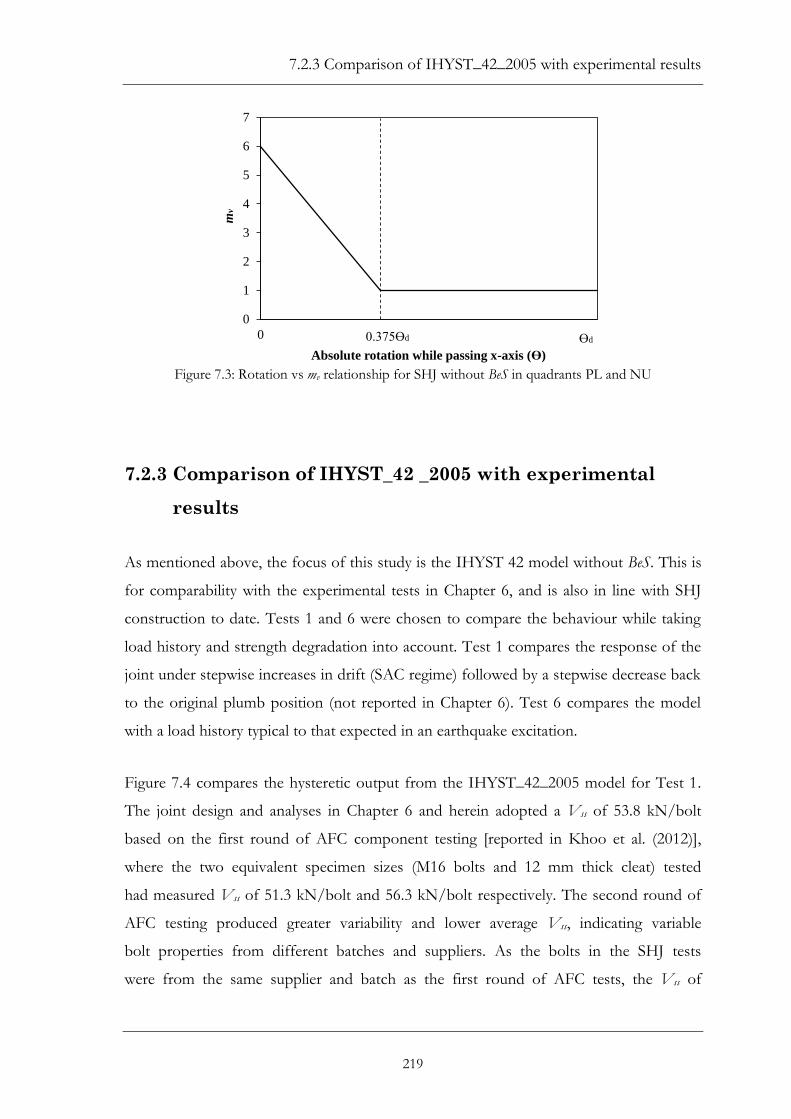
7.2.3 Comparison of IHYST_42_2005 with experimental results
219
Figure 7.3: Rotation vs mv relationship for SHJ without BeS in quadrants PL and NU
7.2.3 Comparison of IHYST_42 _2005 with experimental
results
As mentioned above, the focus of this study is the IHYST 42 model without BeS. This is
for comparability with the experimental tests in Chapter 6, and is also in line with SHJ
construction to date. Tests 1 and 6 were chosen to compare the behaviour while taking
load history and strength degradation into account. Test 1 compares the response of the
joint under stepwise increases in drift (SAC regime) followed by a stepwise decrease back
to the original plumb position (not reported in Chapter 6). Test 6 compares the model
with a load history typical to that expected in an earthquake excitation.
Figure 7.4 compares the hysteretic output from the IHYST_42_2005 model for Test 1.
The joint design and analyses in Chapter 6 and herein adopted a Vss of 53.8 kN/bolt
based on the first round of AFC component testing [reported in Khoo et al. (2012)],
where the two equivalent specimen sizes (M16 bolts and 12 mm thick cleat) tested
had measured Vss of 51.3 kN/bolt and 56.3 kN/bolt respectively. The second round of
AFC testing produced greater variability and lower average Vss, indicating variable
bolt properties from different batches and suppliers. As the bolts in the SHJ tests
were from the same supplier and batch as the first round of AFC tests, the Vss of
0
1
2
3
4
5
6
7
0
mv
Absolute rotation while passing x-axis (Ө)
Ɵd0.375Ɵd

Chapter 7: Analytical studies of the SHJ and SCSHJ
220
53.8 kN/bolt is more representative and therefore used in the analysis. The input
parameters of the joint into RUAUMOKO are given in Appendix C. In practice, bolts
from different manufacturers and batches would be used in the SHJ, which would
produce variable capacities similar to that found in the AFC tests described in Chapter 4.
They would also produce mean moment capacities that are lower than the SHJ and
SCSHJ tests presented in Chapter 6.
Figure 7.4: Comparison between Test 1 and IHYST_42_2005 model under the SAC regime (only
response from cycles in green)
Under cycles of rotations below 10 mrad, the model underestimated the joint strength
and stiffness at load reversal. This is because the model represents the load reversal
behaviour with a constant overshoot of C2MSHJ,y (0.1MSHJ,y for the SHJ without BeS) past
the x-axis at all levels of rotation followed by the stiffness of mvrpllkSHJ,o as described
above. The experimental result on the other hand had a significantly higher overshoot at
lower levels of rotation, which then decreased as the rotational amplitude increased. As a
result, the accuracy of the model improved with increasing rotational amplitudes as the
experimental overshoot decreased to the similar level of the model. The IHYST_42_2005
gave a reasonably good overall representation of the SHJ behaviour under increasing
levels of rotation in the SAC loading regime. It was shown to be within 10% of MSHJ,y,
-300
-200
-100
0
100
200
300
-30 -20 -10 0 10 20 30
Mom
ent
(kN
m)
Rotation (mrad)
Experimental results
IHYST_42_2005
-30
-20
-10
0
10
20
30
0
Ro
tati
on
(m
ra
d)
Time

7.2.3 Comparison of IHYST_42_2005 with experimental results
221
MSHJ,25 and MSHJ,0 (Chapter 6). However, the comparison had yet to be made under
decreasing cycles of rotation or under a load history similar to an actual earthquake.
Following the SAC loading regime [Figure 6.11(a)] applied in Test 1, the specimen was
immediately subjected to a further displacement regime comprising stepwise decreases in
drifts to zero. The actual purpose of this sequence was to return the column to a vertical
position with minimal residual stress for ease of dismantling the connection AFCs. It was
then found to be suitable to determine the accuracy of the IHYST_42_2005 model in
predicting joint stiffness and strength degradation under cycles of decreasing amplitudes.
Figure 7.5 compares the measured and predicted responses from the final cycle in the
SAC regime (to the maximum rotation of approximately 26 mrad), followed by the
stepwise decreases in rotation to approximately zero. The load history is shown in the
inset of Figure 7.5. In the experimental tests, the joint continued to load along the spine
curve as it was pushed into the PU quadrant immediately following the cycle of
maximum rotation to 26 mrad. At load reversal, which occurred at approximately 6 mrad,
the resistance built up at a significantly lower stiffness compared to the IHYST_42_2005
model (as seen in quadrant PL). The experimental curve eventually reached
approximately -67 kNm in quadrant NL with a total travel of approximately 15 mrad in
the negative direction. The stiffness was similar to the joint response when the load was
reversed at the maximum drift of 26 mrad in the previous cycle. At load reversal from
26 mrad positive rotation, the joint built up to -72 kNm in 15 mrad of travel in the
negative direction, before increasing in stiffness as the bolts in the AFC go into double
curvature and thus developing the stable sliding resistance. In the case of the winding
down cycles, there was insufficient sliding distance for the joint to develop the stable
sliding resistance. The stiffness comparison is shown in Figure 7.5. When the load was
reversed again in the NL quadrant, and the connection was pushed in the positive
rotation direction (and into quadrant NU), the stiffness was again significantly lower than
the IHYST_42_2005 model prediction. As the joint was subjected to further cycles, it
generally loaded along the same line. This means that there was a slight re-stiffening of
the joint, as it would load to the equivalent -67 kNm (as before) in 9 mrad negative
rotation from the zero position. The measured results of Test 1 also showed a difference
in positive and negative rotations, with higher stiffness in the positive rotation as shown

Chapter 7: Analytical studies of the SHJ and SCSHJ
222
in Figure 7.5 (ie. kp > kn). The reason for this is unknown, as the rotations presented are
the average of both North and South side joints (as described in Chapter 6). Any
directional effects would have been cancelled.
The experimental results indicate that the joint undergoes permanent losses in strength
and stiffness as a function of maximum ductility. The IHYST_42_2005 model however,
does not pick up the permanent softening, resulting in unrealistic increases in stiffness
when the joint winds down. This is because mv is determined from the ductility at that
point (ie. just Ө) for quadrants PL and NU (as illustrated in Figure 7.2). Whereas when
the load reverses and loads into quadrants PU and NL, the mv is calculated as a function
of Өp and Өn respectively. This causes mv and the resulting stiffness at load reversal (from
quadrants NL to NU or PU to PL) to reduce when the rotations increase (as seen in the
SAC loading regime comparison), but increase again when Ө decreases. This results in
significant overestimation of the joint strength and stiffness once softening has occurred
at high levels of rotational demand, which is not representative of the actual joint
behaviour. Modifications are required to take permanent joint softening into account.
Figure 7.5: Comparison between Test 1 and IHYST_42_2005 model under winding down cycles
(response from cycles in green)
-300
-200
-100
0
100
200
300
-30 -20 -10 0 10 20 30
Mo
men
t (k
Nm
)
Rotation (mrad)
Experimental results
IHYST_42_2005
k
≈15 mrad
≈15 mrad
≈9 mrad
k≈ -67 kNm
p
n
-30
-20
-10
0
10
20
30
0
Rota
tion
(m
rad
)
Time

7.2.4.1 Proposed modifications to IHYST 42
223
7.2.4 Modifications to SHJ model (IHYST 42)
7.2.4.1 Proposed modifications to IHYST 42
Tests 1 and 2 were the only tests with the standard SHJ, where the behaviour was
contributed by the AFCs alone. However, Test 2 was subjected to extreme near-fault
type deformations, as opposed to the SAC cyclic loading, making the rotational
behaviour difficult to interpret. While the other SCSHJ tests (Test 3, 4 and 7) were also
subjected to the stepwise decreases in drift to reduce residual stresses at the end of the
SAC regime, attempts to isolate the AFC contribution from the ring spring contribution
did not provide meaningful results. Consequently, the proposed modification was made
based only on the observations from Test 1, namely: (1) the overshoot moment at load
reversal is higher when the peak demand is lower and (2) the stiffness at load reversal
under lower amplitude cycles that occur after a larger amplitude cycle is similar to that at
the larger amplitude. The modification is shown in Figure 7.6 and is summarised as:
1. The factor C2 applied to the moment overshoot is not a constant, but
instead calculated as a function of rotation (Ɵ). C2 starts at 1.0 at
Ɵ = 0, and decreases to 0.1 at Ɵ = C5Ɵ. It then remains at 0.1 with
further increases in Ɵ. This takes the strength and stiffness degradation
as a function of rotation into account. The C2 factor is calculated at
each instantaneous point (C2,cal) and written as:
( ) (7.8)
2. The value of C2 applied is set equal to the minimum of the calculated
value from the instantaneous rotation, or the minimum value
previously reached under the loading history. This takes permanent
softening of the joint into account. The applied C2 can thus be written
as Equation 7.9 where: C2,cal = calculated from Equation 7.8; C2,min =
minimum C2 in the duration of the loading history
( ) (7.9)

Chapter 7: Analytical studies of the SHJ and SCSHJ
224
3. The stiffness at load reversal is constant at rpllko (ie. mv no longer
applied as the stiffness loss is captured in the variable C2 moment
overshoot factor).
It is also expected that the constant C5 should in reality be a variable that is dependent on
the beam depth. This is because the beam depth determines the relationship between
joint rotation and the level of AFC sliding, which in turn determines the joint strength
and stiffness loss. There is currently insufficient full-scale SHJ testing to establish this and
it is recommended as a focus for future research.
Figure 7.6: Proposed changes to IHYST 42 model (changes shown in red)
The modification is illustrated in Figure 7.7 which shows the SHJ pushed to excursions
passing the x-axis (Ө) at 3 mrad, -8.5 mrad, 26 mrad, -26 mrad, 5 mrad, -5 mrad and to
26 mrad. This corresponds to two excursions below C5Өd, followed by a large cycle
exceeding C5Өd, a cycle below C5Өd and ending with a large excursion. When the joint is
first pushed from the zero displacement, it loads along the same path as IHYST_42_2005
till 3 mrad rotation. At load reversal, it unloads along line rluko as before but with an
Mo
men
t
Rotation
MSHJ,0
kSHJ,in = rsp kSHJ,o
MSHJ,y
MSHJ,0
rlu rpll kSHJ,o
rlu rpll kSHJ,o
rpll kSHJ,o
kSHJ,o
ru kSHJ,o
ru kSHJ,o
rpll kSHJ,o
MSHJ,y
kSHJ,in = rsp kSHJ,o PLNL
PUNU
C2 MSHJ,y
C2 MSHJ,y

7.2.4.1 Proposed modifications to IHYST 42
225
overshoot of C2MSHJ,y, where C2 = max[0.1,1–0.9×3/(0.375×30)] = 0.7479. The joint
then loads with stiffness rpllko till it reaches MSHJ,y. After which, it loads along rlurpllkSHJ,o as
for the IHYST_42_2005 model till it reaches the spine curve. It then loads along kSHJ,in
till -8.5 mrad. The load then reverses, with an overshoot calculated with C2 = max[0.1,1–
0.9×8.5/(0.375×30)] = 0.2857. It then loads to a cycle to 26 mrad in both positive and
negative rotations, which is the same curve as for IHYST_42_2005, where C2 is at the
minimum of 0.1 as abs(Ө)>C5Өd. The behaviour of the joint after the moment overshoot
is the same throughout, where the joint loads along rpllko till the moment reaches MSHJ,y,
followed by rlurpllkSHJ,o to the spine curve. The final cycle of 5 mrad shows the changes to
the strength degradation and load history dependence of the model. At the start of the
final cycle (point shown as O) the joint loads along the spine curve into quadrant PU till
load is reversed. As the joint is pushed in the negative direction into quadrant PL, the
moment overshoot is equal to the minimum value previously reached (ie. C2 = 0.1 as for
the previous cycle). Under a lower amplitude displacement, it lacks sufficient sliding
distance to develop the stable sliding capacities (reach the spine curve) before the load is
again reversed in quadrant NL. When pushed back in the positive direction, the
overshoot is again at the minimum (C2 = 0.1). This time with sufficient sliding distance to
26 mrad, it increases to rlurpllkSHJ,o at MSHJ,y, and eventually the spine curve once more in
quadrant PU.
Figure 7.7: Modifications to calculation of C2 in the model
-30 -20 -10 0 10 20 30Mom
ent
Rotation
(3) Ө > 0.357Өd
→ C2 = 0.1
(5) & (6)
C2 = min (C2,cal, C2,min)
= min (0.58, 0.1)
= 0.1
O
(1) Ө = 3 mrad
→ C2 = 0.7479
(2) Ө = -8 mrad
→ C2 = 0.2857
(4) C2 = 0.1

Chapter 7: Analytical studies of the SHJ and SCSHJ
226
The comparison of the proposed modified model with the experimental results of Test 1
is shown in Figure 7.8. Despite the changes, it can be seen that the model still
overestimates the joint strength and stiffness at decreasing cycles of rotation, although to
a lesser degree than previously. This is similar to the joint at load reversal from the
maximum rotation of approximately 26 mrad, where the stiffness is also initially
overestimated in the model, which then converges to the experimental results as the
connection stiffness increases when it is pushed further in the opposite direction. The
softening may be dependent on the specimen size as the experimental testing by Clifton
(2005) showed that there is limited re-stiffening when the cyclic amplitudes decrease.
Also in Test 1, the joint loaded along the same line as it decreased from cyclic amplitudes
of 6 mrad as described before, indicating limited re-stiffening. The extent of re-stiffening
is unclear from the current available information. In addition to that, the modification
assumes that there is no directional difference in softening (eg. when the joint softens
when loaded in the positive direction, it also loses stiffness when loaded in the negative
direction). There was no evidence from the results of this test or previous tests to
support this assumption. Further experimental testing of full scale beam-column
subassemblies are required to further improve the SHJ hysteretic model.
Figure 7.8: Comparison of proposed model with experimental results
-300
-200
-100
0
100
200
300
-30 -20 -10 0 10 20 30
Mom
ent
(kN
m)
Rotation (mrad)
Experimental results
IHYST_42_2005
-30
-20
-10
0
10
20
30
0
Rota
tion
(m
rad
)
Time
IHYST_42_2012

7.2.4.2 Current modifications (IHYST_42_2012)
227
7.2.4.2 Current modifications (IHYST_42_2012)
The IHYST_42_2005 model was written in Visual Basic and converted to Fortran code
for use in RUAUMOKO. Revision of the model in RUAUMOKO was not within the
scope of this project. However, an attempt was made at modifying the code to meet the
required changes described in Section 7.2.4.1. This is because the SHJ was shown in
Chapter 5 to be more prone to residual drifts under large rotations. The revised model
(referred to as IHYST_42_2012) and written in a new edition of RUAUMOKO (Carr,
2012) produced two significant effects on the rotational behaviour which can be divided
into the behaviour where the rotation is below C5Өd throughout the load history, and
where the rotation exceeds C5Өd.
The behaviour of the connection prior to the rotation exceeding C5Өd is illustrated in
Figure 7.9, which compares the experimental results with the IHYST_42_2005 and
IHYST_42_2012 models, up to rotations of approximately 15 mrad. The joint behaviour
in the elastic range and loading past the yield moment from the plumb position into
quadrant PU is the same for both models. However, at load reversal, the
IHYST_42_2012 overestimates the stiffness losses at low levels of rotation. This is
because the model assumes a constant overshoot with the minimum C2 = 0.1 regardless
of the instantaneous rotation as it passed the x-axis (Ө) or previous maximum rotation
(Өm). After the moment overshoot, the joint loads along rpllko with the mv factor removed.
As the joint is then pushed from the PL quadrant to the NL quadrant, there is a sudden
spike as it loads along the elastic stiffness ko to MSHJ,y. It then continues loading along
rpllko till either load reversal or the spine curve is reached. This creates a flag-shaped
hysteretic curve which is not representative of the actual SHJ behaviour. While it
underestimates the connection strength and stiffness as well as energy dissipation, this
causes it to over predict the self-centering behaviour of the joint.
Once the maximum rotation (Өm) exceeds C5Өd, the IHYST_42_2005 model develops
the intended rotation behaviour as described in Section 7.2.4.1, taking permanent
softening into account. Figure 7.10 compares the hysteretic response of Test 1 through
the SAC regime and the winding down component of the load history. Under load

Chapter 7: Analytical studies of the SHJ and SCSHJ
228
reversal from the PU to the PL quadrants, the model maintained the minimum C2
overshoot and rpllko as it moved from PL to the NL quadrants. Likewise under load
reversal from the NL to the NU quadrants, the joint increased in strength at a stiffness
corresponding to the minimum C2 and rpllko as it moved from quadrants NU to PU.
Figure 7.9: Comparison of IHYST_42_2005 and IHYST_42_2012 models with Test 1 results for
cycles up to approximately 15 mrad rotations (only green section of load history)
Figure 7.10: Comparison of IHYST_42_2012 model with Test 1 results (SAC and winding down
response)
-300
-200
-100
0
100
200
300
-30 -20 -10 0 10 20 30
Mom
ent
(kN
m)
Rotation (mrad)
Experimental results
IHYST_42_2005
IHYST_42_2012
-300
-200
-100
0
100
200
300
-30 -20 -10 0 10 20 30
Mom
ent
(kN
m)
Rotation (mrad)
Experimental results
IHYST_42_2012

7.2.4.2 Current modifications (IHYST_42_2012)
229
The behaviour of the models is also illustrated in the comparison between the
experimental results of Test 6 in Chapter 6 with the IHYST_42_2005 and
IHYST_42_2012 models. Test 6 was tested with the EQ loading regime [shown in Figure
6.11(c)], consisting of the scaled joint rotational outputs of the frame under the Tabas
and El Centro 1979 ground motions. The outputs were from the analytical studies
described in Chapter 5. The response of the connection is provided separately for the
scaled Tabas and El Centro 1979 components in order to illustrate the model behaviour
with Өm above or below C5Өd. The hysteretic curves are shown in Figure 7.11 and 7.12
respectively. The model comprised the IHYST_42_2005 or IHYST_42_2012 models and
the IHYST 18 model in parallel to account for the AFC and ring spring contributions
respectively, proportioned to the design PRS of 40%. The input data for the IHYST 42
spring was determined from Equations 7.1 to 7.7. The input data for the IHYST 18
spring was determined from the modified RSJ model presented as Equations 6.7 to 6.11
and 6.14 to 6.17 in Chapter 6. The input parameters into RUAUMOKO are provided in
Appendix C.
Under the Tabas rotational history, the IHYST_42_2012 model, and to a lesser degree
the IHYST_42_2005 model underestimated the joint stiffness at load reversal (Figure
7.11). This was not unexpected and is consistent with the comparison of
IHYST_42_2005 with Test 1 described in Section 7.2.3 and IHYST_42_2012 above.
Under the El Centro 1979 component, where the maximum rotation exceeded the
C5Ɵd threshold (ie. Өm>0.357Өd), the model then developed the moment-rotational
characteristics expected in the modified IHYST_42_2012 model. The comparison is
shown in Figure 7.12, which provides a reasonable match with the experimental data.
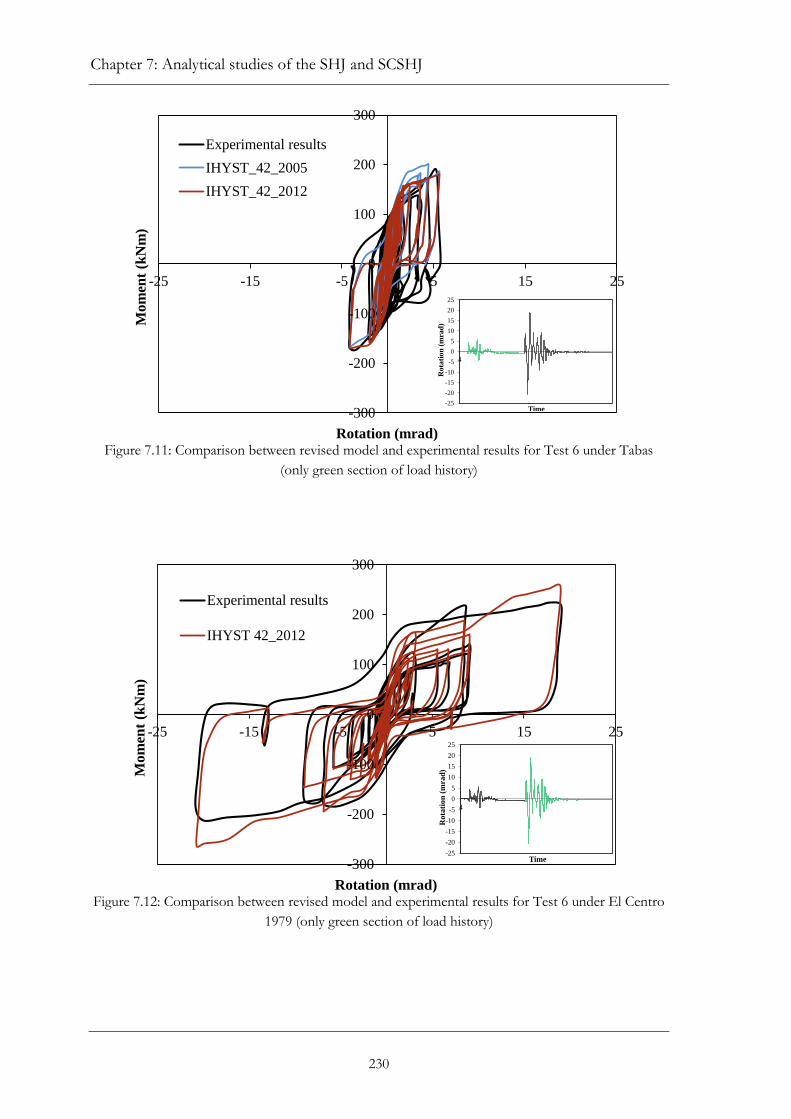
Chapter 7: Analytical studies of the SHJ and SCSHJ
230
Figure 7.11: Comparison between revised model and experimental results for Test 6 under Tabas
(only green section of load history)
Figure 7.12: Comparison between revised model and experimental results for Test 6 under El Centro
1979 (only green section of load history)
-300
-200
-100
0
100
200
300
-25 -15 -5 5 15 25
Mom
ent
(kN
m)
Rotation (mrad)
Experimental results
IHYST_42_2005
IHYST_42_2012
-25
-20
-15
-10
-5
0
5
10
15
20
25
4
Ro
tati
on
(m
ra
d)
Time
-300
-200
-100
0
100
200
300
-25 -15 -5 5 15 25
Mom
ent
(kN
m)
Rotation (mrad)
Experimental results
IHYST 42_2012
-25
-20
-15
-10
-5
0
5
10
15
20
25
4
Rota
tio
n (
mra
d)
Time

7.2.5 Joint modelling discussion
231
7.2.5 Joint modelling discussion
The purpose of this study was to determine the hysteretic model which best represents
the SHJ and SCSHJ for use in time-history analyses. The characteristics/limitations of the
two models IHYST_42_2005 and IHYST_42_2012 can be summarised as:
IHYST_42_2005
Under a rotations below C5Өd, the model underestimates the strength and
stiffness at load reversal due to the assumed constant overshoot of C2MSHJ,y. The
overshoot should be a function of the rotation, representing the bolt tension
losses as a function of ductility.
Stiffness at load reversal in the PL and NU quadrants is determined independent
of maximum ductility reached and therefore does not take permanent softening
into account.
IHYST_42_2012
When the peak rotation does not exceed C5Өd, the model underestimates the
strength and stiffness at load reversal to a higher degree than the
IHYST_42_2005 model. This is due to the minimum constant overshoot of
0.1MSHJ,y, minimum loading stiffness of rpllko and stiffness spike past the zero
position, which results in a flag-shape hysteretic behaviour.
Once the peak rotation exceeds C5Өd, the model provides a reasonable
representation of the SHJ for subsequent cycles, and thus takes permanent
softening under large rotations into account.

Chapter 7: Analytical studies of the SHJ and SCSHJ
232
The IHYST_42_2005 provides a better representation of the joint behaviour compared
to IHYST_42_2012 when the rotational demand is relatively low (ie. Өm < C2Ɵd). In both
cases, the underestimation of the joint strength and stiffness at load reversal may
overestimate the self-centering capability of the joint and also underestimate the
rotational demand. Good self-centering (covered in more detail in Chapters 5 and 6) is
characterised by high resistance in quadrants PU and NL with low resistance in quadrants
PL and NU. The IHYST_42_2005 would however overestimate the joint strength and
stiffness at the end of the earthquake excitation when softening would have occurred.
Once the rotation exceeds the C5Өd threshold, IHYST_42_2012 provides a better
representation of the SHJ by taking permanent softening into account under decreasing
amplitude cycles. This makes it suitable for modelling the joint and frame behaviour
following a severe ground motion shaking. These two models establish upper and lower
bounds of the SHJ behaviour. Due to time constraints, it was decided that both the
IHYST_42_2005 and IHYST_42_2012 models would be used in further analytical
studies in this project. The results can then be compared to give an indication of the
performance of the frames with the SHJ and SCSHJ.
7.3 Time-history analysis
233
7.3 Time-history analysis
Section 7.3 presents numerical integration time-history analyses undertaken to determine
the behaviour of the SHJ and SCSHJ in representative frames using the revised
IHYST_42_2012 and modified RSJ (IHYST 18) models. Analysis with IHYST_42_2005
was also undertaken for comparison. The effects of ring spring arrangement within the
frame were also studied on frames where ring springs were installed only in the external
columns.
7.3.1 Performance objectives
The performance objectives are similar to those described in Chapter 5. Under the 500
year return period DLE event, the joints should provide ductile moment-rotational
characteristics and return the frame to residual drifts within the construction drift
tolerance of 0.2% (Standards New Zealand, 2009). The residual drift threshold of 0.1%
was also used for comparison, which was based on maintenance requirements found in
the Christchurch 2011 earthquake (Clifton et al., 2011). The peak drifts should also be
within 2.5% to limit damage to non-structural elements (Standards New Zealand, 2004).
Under the 2500 year return period MCE event, the frames may exceed the peak drift
damage thresholds of 2.5% while maintaining the integrity of the structure. The frames
are not expected to be within residual drift limits under the extreme MCE events.
The aim of achieving an effectively rigid structure which would remain elastic in a
subsequent serviceability level event (SLE) was not included in the performance
objectives and analyses. This was based on the experimental findings covered in Chapter
4 which showed that there is negligible post-earthquake elastic strength and stiffness in
the AFC without Belleville Springs, concluding that the bolts would have to be replaced
under the DLE event. The results in Chapter 5 then showed that the upper limit design
PRS of 50% was insufficient to remain elastic in the subsequent SLE. It was therefore
concluded that the original objective was unattainable in the SCSHJ unless very large ring
spring sizes were used, which would be unpractical from a cost and construction
perspective.

Chapter 7: Analytical studies of the SHJ and SCSHJ
234
7.3.2 Frame description
Two frame types were studied to provide a range of building sizes expected in SHJ or
SCSHJ construction. The first is the 5-bay longitudinal MRF from the 10-storey Te Puni
Village Tower Building studied in Chapter 5. The building is in Wellington, New Zealand,
corresponding to a high seismic hazard region. It is situated on rock [soil class B to
NZS 1170.5 (Standards New Zealand, 2004)]. The description of the building can be
found in Section 5.3.1, with the layout and member sizes given in Figure 5.7.
The second frame is a 3-bay MRF from a 5-storey prototype building on deep soil (soil
class D to NZS 1170.5), also situated in Wellington. This was the same building studied
analytical by Clifton (2005) in the original development of the SHJ. The building is a
35 m × 21 m office building, with perimeter MRFs along each wall providing lateral
support. The floor is a composite steel flooring system supported by steel secondary
beams. The frame members were designed with the design procedure given in Clifton
(2005), which was modified from the procedure in HERA Report R4-76 (Feeney and
Clifton, 1995). The loadings in the building were in accordance with AS/NZS 1170.1
(Standards New Zealand, 2002), with the steel members designed to NZS 3404
(Standards New Zealand, 2009). The building layout, elevation, member sizes and
summary of loadings are shown in Figure 7.13. The frames studied were based on MRF
1. The perpendicular frames (MRFs 2) are expected to be similar, with the central beam
larger to support gravity loads from the primary beam. The joint moment demands were
determined through a response spectrum model and equivalent static analysis to a
structural ductility factor µf of 4. The natural period of the MRF was 1.41 seconds, with
the second and third modes at 30 and 15% percent respectively. The columns were
assumed to be pinned to the base, with minimum rotational stiffness in accordance to
NZS 3404 (Standards New Zealand, 2009). This eliminated column base hinging. Further
details of the prototype building can be found in Clifton (2005). As described in Section
5.3.1, the location of Wellington was chosen as it has the highest seismic hazard of all
major cities in New Zealand, and also subject to near fault events. Furthermore, the soil
categories of B and C are the same throughout New Zealand, and thus the analyses and
results are applicable for all regions.

7.3.3 Joint design and modelling
235
(a)
5 @ 7m = 35m
3 @
7m
= 2
1 m
MRF 1
(b)
5 @
3.5
m =
17
.5 m
530 UB 82
610 UB 101
610 UB 125
610×299 UB 140
610×299 W 153
610×324 W372
610×324 W307
610×299 W270
610×299 W171
610×178 W82
MRF 1
MRF 2
MRF 2
Primary beams
Gravity columns
Secondary beams
Gfloor = 4.5 kN/m2
Qb,floor = 3.5 kN/m2
Groof = 2.25 kN/m2
Qb,roof = 0.25 kN/m2
Gcladding= 3.5 kN/m
(line load)
Figure 7.13: Floor plan of 5-storey prototype building [modified from (Clifton 2005)]
7.3.3 Joint design and modelling
The joints were designed with the same procedure described in Section 5.3.2 in Chapter
5, and presented in Equations 5.1 to 5.9. This entailed designing the SCSHJ based on the
target percentage (PRS) of moment capacity generated by ring springs. It should be noted
that the sliding shear resistance (Vss) values adopted in the design were based on the
recommendations in Clifton (2007), which was were the most up to date values at the
time the design and analyses were conducted. The bolt model and design values have
since been revised in Chapter 4 and tabulated in Appendix A. As the recommended
strength reduction factor (ɸAFC) is 0.70, the effect would have been overall stronger joints
which would reduce the effective frame ductility. It may also have resulted in larger
column sections in capacity design.

Chapter 7: Analytical studies of the SHJ and SCSHJ
236
The SCSHJ studied in Chapter 7 is modified slightly from the joint studied and tested in
Chapters 5 and 6. It involves using two ring springs per SCSHJ, each attached above the
bottom flange of the beam on either side of the beam web. The layout is shown in Figure
7.14. While two ring springs per joint would increase the cost, the ring spring under the
beam bottom flange may not be practical due to aesthetic/architectural issues. The new
configuration would also eliminate the need for the expensive column detailing used for
the large-scale test described in Chapter 6, which involved cutting out part of the column
web to accommodate the centrally placed rod and nuts. The joints were designed with
the proposed modified configuration to determine the likely ring spring sizes required. As
the joints were designed to the target PRS, there would effectively be no significant
difference to the joint properties and behaviour had the configuration been the same as
the original recommendations.
eRS
Figure 7.14: SCSHJ with two ring springs above bottom flange plate

7.3.3 Joint design and modelling
237
Three frames of each 10-storey and 5-storey MRFs were designed and analysed with
different ring spring contributions or arrangements. The frames studied are named
Frames 1, 6 and 7 for the 10-storey MRFs, and Frames A, B and C for the 5-storey
MRFs. Frame 1 is the same as Frame 1 in Chapter 5, which is the 10-storey frame with
the standard SHJ. Frame 6 was designed with SCSHJs in each joint with a target PRS of
25%. This was the same target for Frame 3 in Chapter 5, which was shown to have
residual drifts (δr) under 0.2% for all DLE ground motions. The aim of this analysis was
to determine likely joint and ring spring sizes, and the optimal performance for the given
sizes. It was therefore decided that the ring spring size would be the minimum size
required to generate the target PRS of 25%, which would then be increased to the
maximum achievable PRS. This entailed applying a maximum precompression of 65% of
the spring capacity, which resulted in a larger PRS for each storey level with an average of
30.6%. The number of ring spring elements (ne) was set to ensure the moment at 25 mrad
rotation was within 5% of that in the equivalent joint in Frame 1.
Frame 7 consists of a combination of the standard SHJs in the internal connections and
RSJs in the external connections. They were designed with an average PRS of
approximately 21% over each storey, calculated as the combined MRSJ from the external
columns over the total moment from all joints in the storey level. The purpose of this
was to determine if the frame with the same overall PRS but with ring springs
concentrated at selected joints in the frame also improve self-centering behaviour.
Having the ring springs only at the external column decreases the number of ring springs
required in the frame, which would reduce the cost. It is also easier and cheaper to
fabricate as only the external columns and their respective beam ends need to be detailed
for the ring spring installation. The layout studied would nevertheless limit the overall
storey PRS as a function of the number of bays. The PRS can be increased by adding an
additional SCSHJ or RSJ in the internal connection. This was not within the scope of the
analysis.

Chapter 7: Analytical studies of the SHJ and SCSHJ
238
Frame 7
Frame B
Frame C
SHJ
SCSHJ
RSJ
Figure 7.15: SHJ, SCSHJ and RSJ distribution in Frames 7, B and C.
The 5-storey MRFs were similarly designed to the 10-storey MRF. Frame A was designed
with the standard SHJ. Frame B was designed with the SCSHJ with a target PRS of 25%
per joint. As for Frame 6, Frame B was designed to achieve the maximum PRS with the
minimum ring springs required to generate the target PRS = 25%. This resulted in an
actual PRS ranging from 24.9% to 28.0% in the first four storeys. The 5th storey was a
standard SHJ as the target PRS = 25% was not a practical option given the construction of
the AFC, where a minimum of two rows of bolts in the bottom flange plate is required.
The overall frame therefore had an average of PRS = 20.6%, taking the 5th storey
PRS = 0% into account.
7.3.3 Joint design and modelling
239
Frame C consisted of a combination of SHJ in the internal connections, and SCSHJs in
the external connections, with a target overall PRS = 25% over each storey. As the 5-
storey frame was a 3-bay frame, having RSJs in the external columns would result in
frames with PRS = 33%. The external columns were therefore designed with a
combination of AFC and ring spring contributions, apart from the 5th storey where it was
not practical to have AFCs given the low level of seismic moment demand. The joint
details for the 10-storey and 5-storey frames are summarised in Table 7.2.
The frames were modelled in 2D with the programme RUAUMOKO (Carr, 2007). The
5-storey frames were modelled in similar way to the 10-storey frame, which in turn is the
same to that described in Section 5.4 in Chapter 5. The only difference was the joint
rotational characteristics were modified based on the experimental results as described in
Section 7.2 above. The model does not take the effects of the floor slab into account,
which is particularly large at rotations above 20 mrad as shown in Chapter 6. The SCSHJ
models would therefore likely underestimate the strength and stiffness of the joint, which
would then overestimate the deformation demands in the connections. The enhancement
of the joint strength and stiffness as well as to the self-centering ability of the joint has
yet to be quantified. This research is currently underway at the University of Auckland.

Chapter 7: Analytical studies of the SHJ and SCSHJ
240
Table 7.2: Joint details for Frames 1, 6 and 7, and Frames A, B and C.
Frame Storey
Sliding Component Ring Spring Component PRS
b
(%) MSCSHJ (kNm) Bolt
Vss (kN)
nbfb nwbb MSHJ
(kNm) Typea n
Fpre
(kN) eRS
(mm) MRS
(kNm)
Frame 1 1 M24 75.6 4 3 269 0.0 269
2 M24 75.6 4 3 269 0.0 269
3 M24 75.6 4 3 316 0.0 316
4 M24 75.6 4 3 316 0.0 316
5 M20 47.8 6 3 223 0.0 223
6 M20 47.8 6 3 223 0.0 223
7 M20 47.8 4 3 130 0.0 130
8 M20 47.8 4 3 130 0.0 130
9 M16 30 4 3 64 64
Average 216 Average 216
Frame 6 1 M20 43 6 3 185 13000 20 208 349 72.5 28.2 257
2 M20 43 6 3 185 13000 20 208 349 72.5 28.2 257
3 M20 43 6 3 216 13000 22 208 424 88.2 29.0 304
4 M20 43 6 3 216 13000 22 208 424 88.2 29.0 304
5 M16 27 8 3 143 13000 20 208 350 72.9 33.7 216
6 M16 27 8 3 143 13000 22 208 350 72.9 33.7 216
7 M16 27 6 3 90 10000 20 163 272 44.1 32.9 134
8 M16 27 6 3 90 10000 20 163 272 44.1 32.9 134
9 M20 43 0 4 43 6300 20 70.2 242 17.0 28.1 60
Average 146 Average 63.6 30.6 209
Frame 7c 1 M24 75.6 4 3 269 13000 30 864 304 262 19.6
2 M24 75.6 4 3 269 13000 30 864 304 262 19.6
3 M24 75.6 4 3 316 13000 30 864 379 327 20.6
4 M24 75.6 4 3 316 13000 30 864 379 327 20.6
5 M20 47.8 6 3 223 10000 18 720 318 229 20.4
6 M20 47.8 6 3 223 10000 18 864 305 264 22.8
7 M20 47.8 4 3 130 9000 30 663 223 148 22.1
8 M20 47.8 4 3 130 9000 30 663 223 148 22.1
9 M16 30.0 4 3 64 6300 30 325 204 66.2 20.5
Average 216 Average 226 20.9 224
Frame A 1 M30 110 10 3 941 0.0 941
2 M30 110 8 3 790 0.0 790
3 M30 118 4 4 586 0.0 586
4 M24 74 6 4 466 0.0 466
5 M16 27 4 4 118 0.0 118
Average 580 Average 580
Frame B 1 M30 110 6 3 645 16600 30 455 540 246 27.6 890
2 M24 63 10 4 578 16600 30 420 534 224 28.0 802
3 M24 68 8 3 487 12400 36 260 550 143 22.7 630
4 M20 47 6 3 270 10000 40 163 552 90 24.9 360
5 M16 27 4 4 118 - - - - 0 0.0 118
Average 420 Average 141 20.6 560
Frame Cd 1 M20 40.0 4 3 182 32000 20 1560 463 722 25.9 904
2 M20 40.0 4 0 110 32000 20 1560 457 713 29.7 823
3 M24 68.0 0 3 117 26200 20 1032 481 496 27.8 614
4 M20 47.0 0 3 82 20000 24 612 503 308 23.3 389
5 M16 27 0 0 0 14000 24 325 458 149 38.7 149
Average 123 Average 478 29.1 576 a Two of each per joint b PRS over the storey for Frames 7 and C, for each joint in the other frames c Internal columns are standard SHJs with design shown under the Sliding Component, while the external columns are RSJ with joint design shown in Ring Spring Component d Design shown for the external columns. Internal columns are as for Frame A

7.3.4 Ground motions
241
7.3.4 Ground motions
The same ground motions and scaling factors used in the analyses in Chapter 5 were used
for the 10-storey frame. The suite of ground motions were developed by Oyarzo-Vera et
al. (2012) based on seismological aspects which included magnitude, distances and
earthquake types. The recommended suite consisted of seven accelerograms for both Soil
Class C and D (corresponding to shallow and deep soils) for each region of the North
Island of New Zealand. They were valid for all soil classes provided the reasonable fit
criteria [Clause 5.5.2(c)] in NZS 1170.5 (Standards New Zealand, 2004) is met. The
ground motions were scaled to the DLE and MCE design spectrum for Soil Class B
(rock). There was overlap between the two sets of seven records, with a total of 11 for
the Wellington region. One of the ground motions, which was Lucerne, Landers, USA in
1992, did not meet the criteria of reasonable fit with the target spectra for Soil Class B
and was therefore excluded, leaving the 10 ground motions used in the analyses. Details
of the ground motions can be found in Table 5.2 in Chapter 5.
The suite of 7 earthquake ground motions in Oyarzo-Vera et al. (2012) corresponding to
Soil Class D were used in the analysis of the 5-storey frame. The ground motions and
scaling factors are summarised in
Table 7.3. The ground motion spectra are provided in Figure C-2 in Appendix C.
Table 7.3: Summary of ground motions for 5-storey frame
Earthquake Year Fault
mechanism Original
PGA DLE
Factor MCE Factor
Caleta de Campos, Mexico 19-Sep-85 Subduction 0.141g 2.869 5.164
Duzce, Duzce, Turkey 12-Nov-99 Oblique 0.535g 0.865 1.557
El Centro, Imperial Valley, USA 19-May-40 Strike-Slip 0.347g 1.602 2.884
El Centro #6, Imperial Valley* 15-Oct-79 Reverse 0.439g 1.299 2.338
HKD085, Hokkaido, Japan 26-Sep-03 Subduction 0.283g 1.087 1.957
TCU 051, Chi-Chi, Taiwan* 20-Sep-99 Reverse 0.225g 3.496 6.293
Yarimka YPT, Kocaeli, Turkey* 17-Aug-99 Strike-Slip 0.349g 1.350 2.430
* Forward directivity (near fault) effects

Chapter 7: Analytical studies of the SHJ and SCSHJ
242
7.3.5 Results
The response parameters are similar to Section 5.5.2, which were chosen to evaluate the
damage to both structural and non-structural elements during an earthquake shaking.
They are the peak inter-storey drift (δp), peak roof displacement (Δp) and residual inter-
storey drift (δr). As noted before, the residual joint strength (SR) parameter was not
considered in this analysis. The δp and δr damage limits are 2.5% and 0.1% or 0.2%
respectively under the DLE event as described in Section 5.2.4. Table 7.4 summarises the
overall performance under the DLE and MCE ground motions. The results from both
IHYST_42_2005 and IHYST_42_2012 models are presented with the latter in brackets.
As described in Section 7.2.5, the IHYST_42_2005 model is more representative of the
actual joint behaviour under peak rotational demands not exceeding C5Өd, and the
IHYST_42_2012 model is more representative when the peak rotational demand exceeds
C5Өd. It was generally the case that the rotational demand was lower than C5Өd for all
joints within the frame under the DLE ground motions and exceeded it for majority of
joints within the frames under the MCE. The results are therefore discussed accordingly,
with the DLE results from IHYST_42_2005 and MCE from IHYST_42_2012.
Table 7.4: Summary of results under DLE and MCE ground motions for Frames 1, 6, 7, A, B and C – mean δp, δr, Δp, and number of ground motions exceeding damage thresholds
Frame
Design level earthquake (DLE) Maximum considered event (MCE)
δp (%)
δr (%)
∆p (mm)
np2.5 nr0.1 nr0.2 δp δr (%) ∆p
(mm) np2.5 nr0.1 nr0.2
Frame 1 1.56
(1.55) 0.12
(0.04) 331
(329) 1
5 (1)
1 (0)
3.19 (3.23)
0.66 (0.48)
614 (585)
4 10 (8)
(10) 4
Frame 6 1.55
(1.49) 0.10
(0.04) 320
(326) 1
3 (1)
2 (0)
3.14 (3.19)
0.36 (0.37)
580 (601)
4 10 (8)
5 (3)
Frame 7 1.54
(1.55) 0.08
(0.05) 328
(326) 1
2 (1)
0 3.24
(3.29) 0.37
(0.47) 595
(614) 5 7
4 (5)
Frame A 2.16
(2.11) 0.16
(0.13) 291
(296) 3
(2) 3
(4) 3
(1) 3.90
(3.93) 0.41
(0.41) 610
(618) 6
7 (6)
5 (4)
Frame B 2.11
(2.08) 0.09
(0.08) 294
(296) 2
3 (1)
1 (1)
3.82 (3.92)
0.27 (0.30)
599 (621)
6 5
(6) 5
(4)
Frame C 2.05
(2.02) 0.09
287 (291)
1 (0)
3 (1)
1 (1)
3.76 (3.80)
0.21 (0.27)
585 (590)
6 3
(4) 2
(2) Note: values provided for both IHYST 42 models. The values in brackets are for the IHYST_42_2012 model.
If only one value given, it is the same for both models.

7.3.5.1 Design level earthquake
243
7.3.5.1 Design level earthquake
The performance of the frames under the DLE described and presented here in Section
7.3.5.1 is from the IHYST_42_2005 model.
The mean peak drift (δp) was between 1.54 to 1.56% for Frames 1, 6 and 7, which is well
below the damage threshold of 2.5%. All three frames only exceeded 2.5% under the El
Centro 1979 ground motion, out of all 10 ground motions. The mean δp and distribution
is given in Figure 7.16(a), showing a similar distribution. This was reflected in the similar
peak roof displacement (∆p) for each frame, ranging from 320 to 331 mm. Likewise, the
deformation demands of the 5-storey frames were similar, with the mean δp between 2.05
to 2.16%, and ∆p between 287 to 291 mm for Frames A, B and C. The mean and
distribution of δp is presented in Figure 7.16(b). The demand was higher than the
10-storey frame, with the number of ground motions exceeding the damage threshold of
2.5% (np2.5) at 3, 2 and 1 for Frames A, B and C respectively, out of the 7 ground motions
used in the analyses of the 5-storey frames. This is not unexpected given that the 5-storey
frames were designed to a ductility of 4, as opposed to the ductility of 2 in the 10-storey
frame (Section 5.3.2). The similar peak drift demands is consistent with Chapter 5, where
it was found that the frame peak displacements were independent of PRS.
Figure 7.17(a) presents the mean and distribution of δr for the 10-storey frames.
The mean residual drifts for Frames 1, 6 and 7 were 0.12%, 0.10% and 0.08%
respectively. The number of ground motions exceeding the damage thresholds of 0.1%
(nr0.1) and 0.2% (nr0.2) were 5 and 1 for Frame 1. For Frame 6, the numbers of ground
motions exceeding damage thresholds reduced to nr0.1 = 3 and nr0.2 = 2, and for Frame 7,
the number of ground motions reduced to nr0.1 = 2 and nr0.2 = 0. The improvement in
performance can also be seen in the mean δr over the height of the building, which is
presented in Figure 7.18(a). Frame 1 with the SHJ had the highest average δr, particularly
at the upper stories, which reduced in Frames 6 and 7. There may also be an advantage of
having RSJs in the external columns, as the residual drifts in Frame 7 were lower than
that of Frame 6, despite having a lower average storey PRS of 21% compared to the
average PRS of 30.6% per joint in Frame 7.

Chapter 7: Analytical studies of the SHJ and SCSHJ
244
Figure 7.17(b) presents the mean and distribution of δr for the 5-storey frames. The mean
residual drift for Frame A was 0.16%, with the mean for Frames B and C both at 0.09%.
For Frame A, the nr0.1 and nr0.2 were both 3. The nr0.1 and nr0.2 were 3 and 1 respectively
for both Frames B and C. The mean δr over the height of the building is shown in
Figure 7.18(b), which shows an overall reduction in residual drifts over the height of the
building in Frames B and C. However, the residual drifts were overall higher than the
10-storey frame, which is probably due to the greater drift demand that they were
subjected to. The results nevertheless showed that the performance improved with the
ring springs, with little difference between Frames B and C.
(a) 10-storey DLE peak drifts
(b) 5-storey DLE peak drifts
(c) 10-storey MCE peak drifts
(d) 5-storey MCE peak drifts
Figure 7.16: Frame peak drift distribution: (a) 10-storey DLE, (b) 5-storey DLE, (c) 10-storey MCE
and (d) 5-storey MCE
0.001.002.003.004.005.006.007.008.00
0 5 10 15 20 25 30 35 40 45 50Max
imu
m d
rift
(%
)
PRS (%)
Individual records Mean
2.5% 0.0
0.5
1.0
1.5
2.0
2.5
3.0
3.5
0 10 20 30 40
Pea
k d
rift
(%
)
Frame
2.5% damage threshold
761
0.0
0.5
1.0
1.5
2.0
2.5
3.0
3.5
0 10 20 30 40
Pea
k d
rift
(%
)
Frame
2.5% damage threshold
CBA
0.0
1.0
2.0
3.0
4.0
5.0
6.0
7.0
8.0
0 10 20 30 40
Pea
k d
rift
(%
)
Frame
2.5% damage threshold
7610.0
1.0
2.0
3.0
4.0
5.0
6.0
7.0
8.0
0 10 20 30 40
Pea
k d
rift
(%
)
Frame
2.5% damage threshold

7.3.5.1 Design level earthquake
245
Figure 7.17: Frame residual drift distribution: (a) 10-storey DLE, (b) 5-storey DLE, (c) 10-storey
MCE and (d) 5-storey MCE.
(a) 10-storey DLE residual drifts
(b) 5-storey DLE residual drifts
(c) 10-storey MCE residual drifts
(d) 5-storey MCE residual drifts
0.001.002.003.004.005.006.007.008.00
0 5 10 15 20 25 30 35 40 45 50Max
imu
m d
rift
(%
)
PRS (%)
Individual records Mean
2.5% 0.00
0.05
0.10
0.15
0.20
0.25
0.30
0.35
0.40
0 10 20 30 40
Res
idu
al
dri
ft (
%)
Frame
0.1% and 0.2%
damage
thresholds
1 6 7
0.00
0.10
0.20
0.30
0.40
0.50
0 10 20 30 40
Res
idu
al
dri
ft (
%)
Frame
0.1% and 0.2%
damage
thresholds
CBA
0.00
0.50
1.00
1.50
2.00
2.50
3.00
0 10 20 30 40
Res
idu
al
dri
ft (
%)
Frame
0.1% and 0.2%
damage thresholds
7610.00
0.20
0.40
0.60
0.80
1.00
1.20
1.40
1.60
1.80
0 10 20 30 40
Res
idu
al
dri
ft (
%)
Frame
0.1% and 0.2%
damage thresholds
CBA

Chapter 7: Analytical studies of the SHJ and SCSHJ
246
(a) 10-storey DLE
(b) 5-storey DLE
(c) 10-storey MCE
(d) 5-storey MCE
Figure 7.18: Mean storey drift distribution (a) 10-storey DLE, (b) 10-storey MCE, (c) 5-storey DLE
and (d) 10-storey MCE
0
1
2
3
4
5
6
7
8
9
10
0 0.05 0.1
Sto
rey
Residual drift (%)
0
1
2
3
4
5
0 0.1 0.2
Sto
rey
Residual drift (%)0
1
2
3
4
5
0 0.5
Sto
rey
Residual drift (%)
Frame 1 - IHYST_42_2005
Frame 6 - IHYST_42_2005
Frame 7 - IHYST_42_2005
Frame 1 - IHYST_42_2012
Frame 6 - IHYST_42_2012
Frame 7 - IHYST_42_2012
Frame A - IHYST_42_2005
Frame B - IHYST_42_2005
Frame C - IHYST_42_2005
Frame A - IHYST_42_2012
Frame B - IHYST_42_2012
Frame C - IHYST_42_2012
0
1
2
3
4
5
6
7
8
9
10
0 0.1 0.2 0.3 0.4 0.5
Sto
rey
Residual drift (%)
0
1
2
3
4
5
0 0.2 0.4
Sto
rey
Residual drift (%)

7.3.5.2 Maximum considered earthquake
247
7.3.5.2 Maximum considered earthquake
The performance of the frames under the MCE described and presented here in Section
7.3.5.2 is from the IHYST_42_2012 model unless stated otherwise.
Figure 7.16(c) presents the mean δp and distribution of the 10-storey MRFs under the
MCE ground motions. Note that this is different from that reported in Chapter 5 due to
the IHYST_42_2012 used here. The mean δp was between 3.19% to 3.29%, and the mean
peak roof displacement (∆p) was between 585 mm to 614 mm, again showing limited
effects on the drift demand with ring springs. Figure 7.16(d) presents the δp mean and
distribution of the 5-storey MRFs under the MCE ground motions. The mean δp was
3.80% to 3.93%, and the ∆p was between 590 mm to 621 mm for Frames A, B and C,
showing the similar drift responses of the 5-story frame. The 10-storey frames were again
susceptible to high drift demands under Arcelik and El Centro 1979, as they hit
resonance under these high velocity ground motions scaled to the MCE level (reported in
Chapter 5). However, unlike the results in Chapter 5 where the drifts increased with PRS
for the Arcelik ground motion (Section 5.6.1.2), there was no correlation for the frames
studied in Chapter 7 despite the different average PRS values of 0%, 30.6% and 20.9%
respectively. The reason for this is unclear, and further studies are recommended to
investigate the potential increase in drifts with increasing PRS.
The mean δr and distribution in the 10-storey MRFs under the MCE ground motions is
presented in Figure 7.17(c). As was shown in Chapter 5, the reductions in δr to within the
damage thresholds were limited by high levels of δp. There was nevertheless the trend of
increased self-centering with when the ring springs were used. Frame 1 had the highest
mean with δr = 0.48%, nr0.1 = 8 and nr0.2 = 4. The mean δr reduced to 0.37% for Frame 6,
with nr0.1 = 8 and nr0.2 = 3. The ring springs however did not improve the performance of
Frame 7, with the mean δr = 0.47%, and nr0.1 = 7 and nr0.2 = 5. The mean δr over the
height of the building is shown in Figure 7.18(c) for the 10-storey frames, showing an
overall reduction in residual drifts in Frame 6 for the PRS of 30.6% per joint, but minimal
effects of the PRS of 20.9% per storey in Frame 7.

Chapter 7: Analytical studies of the SHJ and SCSHJ
248
The mean δr and distribution in the 5-storey MRFS under the MCE ground motions is
presented in Figure 7.17(d). Frame A had the highest mean δr of 0.41%, which reduced to
0.30% and 0.27% in Frames B and C respectively. The nr0.1 and nr0.2 for both Frames A
and B were nevertheless the same at 6 and 4 respectively, which reduced in Frame C to
nr0.1 = 4 and nr0.2 = 2. The mean δr over the height of the building is shown in
Figure 7.18(d), which shows that apart from the 5th storey, Frame A had lower residual
drifts than Frames B and C. This was due to the effects of El Centro 1979 where the
frames hit resonance, which skewed the results, of which the δr distribution over the
height of the frame is shown in Figure 7.19(a). This was the only case where all joints
within any storey exceeded the ductility where the bolts hit the end of the slotted hole
and the bottom flange plate fractures. This corresponds to a rotation of approximately 60
mrad for the 5th storey connection in Frame A. This resulted in large residual rotations in
the 5th storey, and the change to the overall frame behaviour. Figure 7.19(b) shows the
mean δr distribution of the other 6 ground motions, where the performance of Frame B
and C were improved by the ring springs, compared to the performance of Frame A.
While an event like El Centro 1979 may occur, this comparison was made to show that
the trend and benefits of the ring springs were observed in the other ground motion
records.
(a) El Centro 1979 residual
drift
(b) Residual drifts excluding El
Centro 1979
Figure 7.19: 5-storey frame residual drift distribution under the MCE level for (a) El Centro 1979 and
(b) other records excluding El Centro 1979
0
1
2
3
4
5
0 1 2
Sto
rey
Residual drift (%)
0
1
2
3
4
5
0 0.1 0.2 0.3
Sto
rey
Residual drift (%)
0
1
2
3
4
5
0 0.5
Sto
rey
Residual drift (%)
Frame A - IHYST_42_2005
Frame B - IHYST_42_2005
Frame C - IHYST_42_2005
Frame A - IHYST_42_2012
Frame B - IHYST_42_2012
Frame C - IHYST_42_2012

7.3.6 Time-history analysis discussion
249
7.3.6 Time-history analysis discussion
The drift demands were independent of the frame PRS for both the 10-storey and
5-storey frames, under both the DLE and MCE level ground motions. As a low damage
solution, which would include reducing damage to non-structural elements, the peak
drifts should not exceed the limit of 2.5%. This was generally the case for the DLE event
in the 10-storey frames, where np2.5 was 1 for all frames out of the 10 ground motions.
However in the 5-storey frames, np2.5 was 3, 2 and 1 out of the 7 ground motions for
Frames A, B and C respectively. It is recommended that the maximum ductility of 3 is
used in order to limit peak drifts to within 2.5%. This should be studied further with
different frame layouts, heights, and column base conditions.
Under the DLE ground motions, the benefits of ring springs were shown for both the
10-storey and 5-storey frames, where the residual drifts reduced in the frames with ring
springs. In the 10-storey frames, the residual drifts in Frame 7 were slightly lower than
that of Frame 6, despite the lower overall PRS of 20.9% compared to 30.6% in Frame 6.
This indicates there may be advantages of using a combination of SHJ and RSJs within
the frames, compared to an even distribution of PRS across all joints. However, there was
no clear difference between the 5-storey Frame B and Frame C, despite the different PRS
values of 20.6% and 29.1% respectively, and their different ring spring arrangements.
This is illustrated in Figures 7.20 and 7.21, which presents the moment-rotational
response of an internal and an external connection on the 3rd floor of the 5-storey
frames. The internal joints in Frames A and C are identical (Figure 7.20), but the residual
rotation is reduced under dynamic shake-down due to the influence of the flag-shaped
response of the external connection in the same storey (Figure 7.21). The effect of overall
PRS and ring spring distribution may also be dependent on other parameters such as
frame layout and building height, which is recommended for future research.

Chapter 7: Analytical studies of the SHJ and SCSHJ
250
Both the 10-storey and 5-storey frames had large peak and residual drifts under the
ground motions scaled to the MCE events. This was not unexpected as the performance
objective was to maintain the integrity of the structure under rare, extreme MCE events.
While there were reductions in the overall peak residual drifts in the frames with ring
springs (apart from Frame 7), the residual drifts were high, with similar number of
ground motions exceeding the damage thresholds of 0.1% and 0.2%. This is due to the
large peak drifts that the frames were subjected to, which was not unexpected in an MCE
level event.
In the 10-storey frame, Frame 6 performed better than Frame 7, in contrast to their
performance under the DLE ground motions, where Frame 7 had lower residual drifts
than Frame 6. This is likely due to the lower PRS of 20.9% in Frame 7 compared to 30.6%
in Frame 6. There was effectively no difference in the peak residual drifts between
Frames 1 and 7, although the overall mean residual drifts over the height of the frame did
reduce from Frame 1 to Frame 7. In the 5-storey frames, the ring springs reduced the
mean δr in Frames B and C. There was also a reduction from Frame B to C, which could
be due to the larger overall PRS in Frame C. However, it should be noted that in some
cases the frames with ring springs had increased residual drifts or rotations. This is
illustrated in Figures 7.22 and 7.23, which presents the moment-rotational response of
the same joints in Figures 7.20 and 7.21, but under the Caleta ground motion scaled to
the MCE level shaking. It can be seen that while the flag-shaped behaviour of the
external column in Frame C (Figure 7.23) produced near zero residual rotation, this did
not improve the behaviour of the internal connection (Figure 7.22). The internal
connection in Frame A had a lower residual rotation, and an overall lower frame residual
drift.

7.3.6 Time-history analysis discussion
251
Figure 7.20: Moment-rotational response of the internal column on the 3rd storey of the 5-storey
frames under the TCU ground motion scaled to the DLE event
Figure 7.21: Moment-rotational response of the external column on the 3rd storey of the 5-storey
frames under the TCU ground motion scaled to the DLE event.
-1500
-1000
-500
0
500
1000
1500
-6 -4 -2 0 2 4 6 8 10
Mo
men
t (k
Nm
)
Rotation (mrad)
Frame A
Frame B
Frame C
-6
-4
-2
0
2
4
6
8
10
0 20 40 60 80 100Rota
tion
(m
rad
)
Time (s)
-1500
-1000
-500
0
500
1000
1500
-10 -5 0 5 10 15
Mo
men
t (k
Nm
)
Rotation (mrad)
Frame A
Frame B
Frame C
-6
-4
-2
0
2
4
6
8
10
12
0 20 40 60 80 100Rota
tion
(m
rad
)
Time (s)

Chapter 7: Analytical studies of the SHJ and SCSHJ
252
Figure 7.22: Moment-rotational response of an internal column on the 3rd storey of the 5-storey
frames under the Caleta ground motion scaled to the MCE event
Figure 7.23: Moment-rotational response of the internal column on the 3rd storey of the 5-storey
frames under the Caleta ground motion scaled to the MCE event
-1500
-1000
-500
0
500
1000
1500
-25 -20 -15 -10 -5 0 5 10 15
Mo
men
t (k
Nm
)
Rotation (mrad)
Frame A
Frame B
Frame C
-25
-20
-15
-10
-5
0
5
10
15
0 20 40 60 80
Ro
tati
on
(m
ra
d)
Time (s)
-1500
-1000
-500
0
500
1000
1500
-30 -20 -10 0 10 20
Mo
men
t (k
Nm
)
Rotation (mrad)
Frame A
Frame B
Frame C
-30
-25
-20
-15
-10
-5
0
5
10
15
20
0 20 40 60 80
Ro
tati
on
(m
rad
)
Time (s)

7.4 Limitations
253
The results for this analysis indicated that the effectiveness of the ring springs is largely
dependent on the ductility and peak drifts of the frames. In low damage construction, the
frame ductility should be limited to µf = 3, with further studies undertaken to ascertain
the influence of ductility on peak and residual drifts including such factors as the floor
slab contribution to self-centering. It can also be concluded that the use of ring springs
only at selected connections (ie. some RSJs or SCSHJs) with the standard SHJ in other
connections is a viable option at reducing the overall cost of the system while still
providing self-centering benefits.
7.4 Limitations
The frame drift demands for the 10-storey and 5-storey frames were similar across the
different joint designs, as well as for both the IHYST_42_2005 and IHYST_42_2012
models. As the two models establish upper and lower bounds of the SHJ behaviour with
both producing similar drift demands, it can be concluded that the drift results presented
are a reasonable representation of the overall frame behaviour.
The models may however not be fully representative of the frame residual drifts. As
described in Section 7.2.5, the IHYST_42_2005 model overestimates the joint strength
and stiffness at load reversal in quadrants NU and PL during the dynamic shake-down
phase. This is because the model does not take the strength and stiffness reduction with
increasing peak inelastic rotation (which is dependent on the beam depth). The
overestimation of the joint strength and stiffness in these two quadrants NU and PL may
cause an overestimation of the residual drifts, as it overestimates the resistance to
recentering in these two quadrants. An example of this effect is the comparison between
the MCE response of Frame 1 in Chapter 5 (IHYST_42_2005 model), and in Section
7.3.5.2 (IHYST_42_2012 model), where the latter was significantly lower at 0.48% mean
δr compared to 0.66% in Chapter 5. The DLE results herein may therefore overestimate
the residual drifts of the frames.

Chapter 7: Analytical studies of the SHJ and SCSHJ
254
The IHYST_42_2012 gives a reasonable representation of the joint behaviour once C5Өd
is exceeded, which is assumed to occur under the MCE ground motions. However, not
all connections within the frames had peak rotations above C5Өd. For example, in Frame
A where there are 30 joints, the rotational demand varied between the 7 ground motions,
where between 12 and 30 joints exceeded the C5Өd threshold. This would mean that the
joints that exceeded the threshold gave a reasonable representation of actual shake-down
behaviour, while the other connections would produce the flag-shaped like hysteretic
behaviour described in Section 7.2.4.2. This is not representative of the system and can
cause the analysis to be unconservative in the estimation of frame residual drifts. Further
studies of the frame behaviour and residual drifts should be undertaken with the IHYST
42 model revised in accordance to 7.2.4.1.
The IHYST 18 spring that modelled the ring spring contribution was shown to give a
reasonably good prediction of the joint strength and stiffness under a rotation of
20 mrad. Above 20 mrad, the stiffness and strength increased due to the contribution of
secondary element effects such as floor slab effects as described in Section 6.4.6 in
Chapter 6. Under the MCE event, this was often exceeded. For example, the rotational
demand was above 20 mrad for 26 joints out of the 30 joints in Frame B under the El
Centro 1979 MCE ground motion. This would then underestimate the joint strength and
stiffness, and hence overestimate the rotational demand.

7.5 Recommendations
255
7.5 Recommendations
Further experimental work should be conducted to improve the SHJ model, and the
IHYST 42 in RUAUMOKO. The model has thus far been compared to only two SHJ
subassemblage sizes. They are the larger specimen size comprising a 610 UB 101 external
column and a 530 UB 82 beam by Clifton (2005), and the smaller 460 UB 76.6 internal
column and 360 UB 57 beams described in Chapter 6. Further testing of a specimen size
with beam depth above 600 mm is required to determine the performance of an upper
end size, as well as the accuracy of the rotational model. This would cover beam sizes
used in the analytical analyses. The focus should be on investigating the effects of beam
sizes on the C5 value. The testing should also investigate the behaviour of the joint under
decreasing amplitude cycles.
The hysteretic model should be revised in RUAUMOKO or written in other
programmes to determine the effects to the SHJ or SCSHJ systems described herein. The
recommended revisions (dependence of the joint strength and stiffness at load reversal
on maximum inelastic rotation) are detailed in Section 7.2.4.1. Further analyses is also
required to determine the behaviour of different frame heights, layout, PRS and spring
distribution to determine the expected performance/damage under different levels of
ground shaking. Analyses should be conducted to determine the contribution of the floor
slab and other secondary elements to the overall frame performance, which occurs in
both the SHJ and RSJ connections. The enhancement of strength may affect the strength
hierarchy of the frames, resulting in an undesirable failure mechanism (eg. strong beam-
weak column). Research is currently underway to reliably quantify this contribution at the
University of Auckland. Furthermore, the AFC connections may be stronger than the
design strengths due to the low strength reduction (ɸAFC = 0.7) and high overstrength (ɸo
= 1.4) factors [Section 4.3.3 and Clifton (2005) respectively], imposed by the variability in
bolt properties. The sensitivity of the frames to these effects has not been studied in this
research and is recommended for future research. Finally, cost-benefit analysis of the
system should be conducted, comparing the benefits of the ring springs and the likely
amount of maintenance required at different PRS levels.

Chapter 7: Analytical studies of the SHJ and SCSHJ
256
7.6 Conclusions
1. The SHJ model previously developed (IHYST_42_2005) provides a
reasonable representation of the SHJ behaviour when the maximum
rotation does not exceed C5Өd (ie. 0.357Өd for SHJ without springs). It
was recommended that the model is modified to ensure the stiffness at
load reversal is always equal to the minimum stiffness in the duration
of the earthquake excitation.
2. The model was revised to the IHYST_42_2012 model, which gave an
unrealistic flag-shaped hysteretic behaviour up to a rotation of C5Өd.
Once this was exceeded, the model gave a reasonable prediction of the
SHJ behaviour, taking strength and stiffness degradation into account.
The IHYST_42_2005 model is suitable when the rotational demand is
below C5Өd. The IHYST_42_2012 is suitable for joints where the
rotational demand exceeds C5Өd.
3. It is recommended that larger SHJ specimen sizes (above 600 mm
deep beam) are tested to verify the joint behaviour and accuracy of the
IHYST 42 model.
4. The revised IHYST_42_2012 model predicted similar drift demands in
the 10-storey and 5-storey MRFs, but with reduced residual drifts. The
latter is due to the lower stiffness at load reversal, which reduced the
resistance to recentering. It was shown that PRS values between 20% to
30% has minimal effect on the peak drift and reduces residual drifts
under the DLE shaking.
5. The use of ring springs only at the external columns was shown to
improve the overall self-centering ability of the system. The frames
under the DLE shaking performed similarly or better than the frames
with ring springs at every joint. Under the MCE level shaking, there
were no benefits for the 10-storey frame while the 5-storey frame
residual drifts reduced.
7.7 References
257
6. A structural ductility factor of µf = 3 is recommended for low damage
systems. Recommendations for future research on the SCSHJ were
given, which includes further full-scale testing of the SHJ and SCSHJs,
further validation of the hysteretic model, further analysis on different
frame and joint configurations and arrangements, and finally cost-
benefit analysis of the overall system.
7.7 References
Carr, A. (2007). RUAUMOKO2D. Civil Engineering Department, University of
Canterbury, Christchurch, New Zealand.
Carr, A. (2012). RUAUMOKO2D. Civil Engineering Department, University of
Canterbury, Christchurch, New Zealand (specially provided by the author for this
project).
Clifton, G. C. (2005). “Semi-rigid joints for moment-resisting steel framed seismic-
resisting systems.” Department of Civil and Environmental Engineering,
University of Auckland, Auckland.
Clifton, G. C. (2007). Sliding Hinge Joint: Revisions to the Design Procedure. Heavy
Engineering Research Association, Auckland.
Clifton, G. C., Bruneau, M., MacRae, G. A., Leon, R. T. and Fussell, A. (2011). “Steel
structures damage from the Christchurch earthquake series of 2010 and 2011.”
Bulletin of the New Zealand Society for Earthquake Engineering, 44(4): 297-318.
Khoo, H. H., Clifton, G. C., Butterworth, J. W. and MacRae, G. A. (2012). “Shim and
bolt size effects on the Asymmetric Friction Connection.” 7th STESSA Conference
on the Behaviour of Steel Structures in Seismic Areas. Santiago, Chile.

Chapter 7: Analytical studies of the SHJ and SCSHJ
258
Oyarzo-Vera, C. A., McVerry, G. H. and Ingham, J. M. (2012). “Seismic zonation and
default suite of ground-motion records for time-history analysis in the North
Island of New Zealand.” Earthquake Spectra, 28(2): 667-688.
Pantke, M. (2001). “Development of analytical models for SHJ and SHJS.” Report for 2nd
Industrial Internship, Heavy Engineering Research Association, Manukau City,
New Zealand.
Standards New Zealand (2002). AS/NZS 1170.1 - Structural design actions. Wellington,
New Zealand.
Standards New Zealand (2004). NZS 1170.5 - Structural design actions. Earthquake actions.
Wellington, New Zealand.
Standards New Zealand (2009). NZS 3404 - Steel structures standard. Wellington, New
Zealand.

259
Chapter 8
1 Summary and conclusions
This thesis presents research undertaken to address limitations in the low damage Sliding
Hinge Joint (SHJ) research to date, and to develop the self-centering Sliding Hinge Joint
(SCSHJ). The aim of the SCSHJ is to ensure frame residual drifts are within construction
tolerance limits and the joints return to effectively rigid following a design level
earthquake (DLE) shaking. Research on addressing limitations in the existing SHJ is
presented in Chapters 2 to 4 and the development of the SCSHJ is presented in
Chapters 5 to 7.

Chapter 8: Summary and conclusions
260
8.1 Summary
8.1.1 Bottom and top flange plate behaviour
A study on the susceptibility of the bottom and top flange plates to low-cycle fatigue
failure was presented in Chapter 2. The plates were analysed assuming the stress and
strain in the flange plates comprised the effects of axial load, plate curvature and shear
stresses due to joint moment demand, deformation of the flange plates due to joint
rotation, and joint shear respectively. The maximum stress and strain under a rotation of
30 mrad was then calculated for the most critical flange plate sizes designed to the
current design procedure. The number of cycles to failure was estimated using a damage
model previously developed for structural steel plates based on the Coffin-Manson
relationship. Using the theoretical maximum stress and strain, it was predicted that the
critical component is the top flange plate which has cycle life of 458 cycles to 30 mrad
rotation. Applying a safety factor of 5, which is conservative for fatigue assessments, the
cycle life is reduced to 91 cycles which exceeds 3 severe earthquake events, each with 28
cycles to an inelastic sliding rotation of 30 mrad. It was therefore concluded that based
on the limited study undertaken, adequately designed and detailed flange plates in
accordance to the current design provisions are not prone to low-cycle fatigue failure.
The analyses and conclusions reported should be used with caution due to the limitations
of the study. The demands in the bottom and top flange plates were calculated using a
simple model based on geometry. These values have not been validated by experimental
testing or FEA. Experimental testing of the SHJ with measured strains in the flange
plates is recommended for future research, and FEA is recommended to validate the
calculated demands in the SHJ components. No experimental testing was undertaken in
this project to validate the parameters in the Coffin-Manson damage model.
Furthermore, while the model was based on components representative of the SHJ
flange plates, the model was developed based only on 6 tests at two different strain
conditions as detailed in Section 2.4.1. Further testing is required to validate the adopted
parameters.

8.1.2 Dynamic behaviour of steel shims of different hardness
261
8.1.2 Dynamic behaviour of steel shims of different
hardness
Testing of the Asymmetric Friction Connection (AFC) with steel shims was undertaken
to determine their performance under dynamic rates of loading. The results are presented
in Chapter 3. The specimens were tested with sinusoidal cycles up to displacement
amplitudes of 13.8 mm at 0.67 Hz. The average slip rates of the specimens were between
13.8 mm/sec to 36.8 mm/sec. It was shown that within the range of slip rates tested, the
sliding behaviour was independent of rate.
The effects of steel shims of different hardness were tested based on the understanding
that sliding between surfaces of different hardness improves performance. A total of 10
tests were undertaken with shims made of three different steel grades. The shim materials
tested in order of increasing hardness were mild steel (G300), high strength quenched
and tempered steel (G80), and abrasion resistant steel (G400). The average measured
hardness values were 168 HB, 266 HB and 382 HB in the Brinell scale respectively. The
shims were sliding on the cleats which were made of mild steel. Their performance was
evaluated based on the level of frictional resistance, material wear, and the stability and
repeatability of the hysteretic loops. The behaviour was analysed based on the theory of
friction and wear. It was found that (1) adhesion and deformation components of friction
were present in all combinations, (2) there was no correlation between hardness and level
of friction, (3) G400 had the lowest gain in strength, (4) wear reduced with increasing
shim hardness, (5) G400 shims had the most stable and repeatable loops followed by
G80 and G300 shims, (6) G400 shims had the highest and most stable frictional
resistance and the least wear, and are therefore recommended for use in the SHJ, and
(7) Belleville springs increase the friction in the AFCs by reducing bolt tension losses but
do not provide additional improvement to G400 shims in terms of frictional stability.
The bolt model was revised, whereby the lever arm (l) between points of bearing from
the shim plates was modified to shim to shim, ie. l = cleat thickness + shim thickness (Section
3.5.5). The revision was then superseded in Chapter 4 with further testing undertaken
with G400 shims (Section 4.3.2.2 and summarised in Section 8.1.3).
Chapter 8: Summary and conclusions
262
8.1.3 Sliding shear capacity and residual joint strength
Once it was established that abrasion resistant steel (G400) shims are to be used in future
SHJ construction, further testing was conducted to determine the AFC sliding shear
capacities (Vss) and residual joint strengths (SR). A total of 69 tests were conducted to
improve the reliability of parameters used in the bolt model which predicts the Vss as well
as to increase the AFC experimental database. The specimens tested comprised M16 to
M30 bolts and cleat thicknesses of 12 mm to 25 mm. The results are presented in
Chapter 4.
The tension was measured in one bolt in three test specimens which illustrated the drop
in bolt tension due to the interaction of moment-shear-axial actions during sliding. With
the direct measurement of bolt tension and sliding shear friction, the coefficient of
friction (µ) could be determined, giving a recommended value of 0.48. The recommended
lever arm between the points of bearing (l) is estimated to be cleat thickness + 2×shim
thickness based on the examination of the impact marks on the bolt at the end of each test
(Section 4.3.2.2). It should be noted that this supersedes the previous recommendation of
l = cleat thickness + shim thickness (Section 3.5.5 and summarised in Section 8.1.2).
The two revised design parameters (µ and l) were used to compute the bolt model
predicted Vss, which was then compared to the experimental test results. It was shown
that for specimens without Belleville Springs, the revised bolt model matched the
experimental results reasonably well, with the experimental values on average 4% lower
than the computed values and a standard deviation of 15%. There was nevertheless
considerable scatter (as reflected in the high standard deviation) due to the variation in µ
and bolt strengths. The computed bolt model values are recommended for use in design
with a strength reduction factor of 0.70 applied to take the variation into account.
Limited tests of AFCs with Belleville Springs (only M24 bolts) were undertaken,
indicating higher Vss that is independent of lever arm length. Belleville Springs have the
potential to reduce variability in Vss due to their ability to retain and moderate bolt
tension.

8.1.3 Sliding shear capacity and residual joint strength
263
The design Vss values should be used with caution due to the number of limitations in
the research to date. These are summarised as: (1) only three test specimens were used to
estimate the µ, and (2) the l was defined by general observation of impact marks on the
bolts with no statistical basis presented. The current recommendations may therefore be
subject to change with further testing undertaken (as shown in the updates of the l
calculation from Chapters 3 to 4). It is recommended that more tests are conducted to
determine more reliable parameter values with statistical confidence. While a list of
design Vss values was provided for the AFCs with Belleville Springs, the model and
therefore values have not been verified for other bolt sizes apart from the M24 bolts
tested. The AFCs with Belleville Springs should be tested with a range of bolt sizes to
verify the bolt model computed values.
A testing procedure was developed to determine the residual joint strength (SR) of the
AFCs. It was found to be very variable due to its dependency on the position at which
the bolts came to a complete stop. The AFC without and with Belleville Springs had
average SR of 28% and 35.7% calculated as a percentage of their respective Vss. This led
to the conclusion that the bolts should be replaced following a major earthquake and the
SR contribution is considered to be negligible in the SCSHJ covered in Chapters 5
onwards.

Chapter 8: Summary and conclusions
264
8.1.4 Self-centering Sliding Hinge Joint
It was proposed that the self-centering ability of the joint could be improved by
connecting a dual-directional acting ring spring cartridge to the bottom flange of the
beam. The joints can be categorised as the standard SHJ, Ring Spring Joint (RSJ) and
self-centering Sliding Hinge Joint (SCSHJ), which correspond to joints where the flexural
capacities are developed by only the AFC, only the ring spring, and a combination of
both respectively. The development of the SCSHJ is presented in Chapter 5 and
validation of the performance through experimental study presented in Chapter 6.
The RSJ exhibits the ideal flag-shaped static recentering hysteretic curves, which return to
the joints and frame to their pre-earthquake position when the load is slowly released
from the design displacement. A theoretical model of the RSJ hysteretic behaviour was
developed based on the ring spring load-displacement behaviour and the joint
configuration, whereby the ring springs are installed below the bottom flange of the
beam. In the SCSHJ, the ring spring acts in parallel to the AFCs, giving a hysteretic
behaviour that is a combination of the two components. The benefits over the standard
SHJ include (1) the number of bolts in the AFC can be reduced, (2) energy stored in the
spring contributes to joint re-centering upon load removal or reversal, and (3) loss in
joint elastic strength due to bolt tension losses in the AFC can be compensated by ring
spring pre-compression. While the RSJ produces the ideal behaviour, its use is limited by
the high cost of ring springs. The SCSHJ represents a compromise which aims to take
advantage of the energy dissipation, sliding resistance and relatively cheap construction
costs of the SHJ, but include benefits of ring springs to enhance the joint re-centering
ability during dynamic shake-down of a structure. A proposed design procedure was
developed, and is presented in Chapter 5, which involved designing the SCSHJ as a
percentage of joint moment capacity developed by the ring springs (PRS).

8.1.5 Effects of ring spring component in the SCSHJ
265
8.1.5 Effects of ring spring component in the SCSHJ
Time-history analyses on five 10-storey moment resisting frames (MRFs) were
undertaken using a suite of 10 ground motions scaled to the 500 year return period DLE
and the 2500 year return period maximum considered earthquake (MCE). Results are
presented in Chapter 5. The frames were designed to a particular level of PRS for each
joint within the frame. The PRS values studied were 0% representing the standard SHJ
and 15% to 50% representing SCSHJs. While the application of the ring spring at every
joint in a 10-storey frame is unlikely due to cost, this range was studied to determine the
effects of PRS on the system performance over a range of levels. The joints were
modelled using the SHJ model developed in previous research, and the flag-shaped RSJ
model developed.
The PRS had no effect on peak displacement for all ground motions at either DLE or
MCE levels, with the exception of the performance under the Arcelik MCE ground
motion, where the peak displacements increased with increasing PRS. The behaviour
under the Arcelik MCE may indicate a potential sensitivity of peak drift demands to PRS.
Further studies are recommended to investigate this effect. The residual drifts of frames
decreased with increasing PRS. When subjected to the DLE ground motions, the frames
with a minimum PRS of 25% were within construction tolerances of 0.2% for all
earthquake records and frames with PRS of 40% were generally within 0.1%. The
reduction in residual drifts is due to the ring springs increasing the pinching of the
moment-rotational curve which effectively reduces the resistance to recentering. Self-
centering is further enhanced by the reduction in strength and stiffness in the AFC which
results in the hysteretic loops becoming more flag-shaped under decreasing cycles of load
during dynamic shake-down. The recommended level of ring spring contribution is 40%
for a quick return to service. There were no benefits of pinching when the peak drifts
were large (beyond 2.5%). The ground motions where this occurred were the Arcelik and
El Centro 1979 ground motions scaled to the MCE. These ground motions represent
rare and extreme events, where the frames are expected to be damaged while maintaining
the integrity of the structure. It should be noted that the joint rotational models used in
this series of time-history analyses have since been modified using further experimental

Chapter 8: Summary and conclusions
266
tests results in Chapters 6 and 7 to better represent actual joint behaviour. The model
used in Chapter 5 provides a reasonable representation of the rotational demands, but
overestimates the self-centering ability of the joint. This means that the analysis and
conclusions in Chapter 5 are unaffected with regards to peak drifts, but are likely to have
underestimated the residual drifts and self-centering performance of the frames. These
modifications are summarised in Sections 8.1.6 and 8.1.7 below.
The residual joint strength (SR) can also be increased by increasing PRS, which increases
the proportion of joint elastic strength and stiffness contributed by the ring spring. The
joints with higher PRS retain a larger portion of the original elastic joint strength and
stiffness as the ring springs do not undergo degradation like the AFCs when subjected to
inelastic deformation. However, a larger level of PRS beyond the 50% studied is required
to increase the SR whereby the joints remain rigid in a subsequent SLE event once
subjected to a prior DLE event. A higher PRS would require larger and/or more springs
which is difficult to implement given the space required for the springs and the increased
cost, making it impractical to achieve full joint rigidity post-DLE shaking.

8.1.6 Experimental behaviour of full-scale SHJ and SCSHJ
267
8.1.6 Experimental behaviour of full-scale SHJ and SCSHJ
Experimental tests of SHJ and SCSHJs were undertaken on a full-scale joint subassembly
representing an internal connection and are reported in Chapter 6. The test specimen
consisted of a 460 UB 76.6 column and two 360 UB 57 beams. The member sizes were
adopted from the 8th storey of the 10-storey MRF studied analytically in Chapter 5. A
steel deck concrete slab was installed on top of the specimen, over the length of the
beams.
The PRS was varied from 0% to 100%, corresponding to the standard SHJ, RSJ and the
SCSHJ in between. The joints showed stable and repeatable hysteretic behaviour with
minimal damage to the floor slab. The self-centering capability increased with PRS, where
joints with PRS of 100% exhibited the flag-shaped static recentering behaviour. However,
the next highest PRS of 52.3% was insufficient to develop static recentering properties.
The tests also compared the response under seismic-dynamic and quasi-static rates of
loading, showing negligible difference in behaviour. The specimen was also tested to a
near fault pulse type motion to a drift of 5.37%, which resulted in a reduction in lateral
strength of approximately 20%. The connections were not tested to failure, and as such
further experimental testing is required to determine the failure mechanism of the RSJ.
The failure mechanism of the SHJ had previously been demonstrated experimentally to
occur through ductile yielding of the bottom flange plate.
The hysteretic models used in the time-history analyses of the 10-storey frames were
compared to experimental results and presented in Chapters 6 and 7. The ring spring
model (IHYST 18 in RUAUMOKO) was compared to the RSJ tests (only ring spring
contribution) while the SHJ model (IHYST 42 in RUAUMOKO) was compared to the
SHJ test (only AFC contribution). It was found that the ring spring contribution to joint
flexural capacity was underestimated in the hysteretic model used in the analyses reported
in Chapter 5 and summarised in Section 8.1.5 above. This is due to the effects of
secondary element contribution that were not taken into account. The model was
modified with empirically determined constants, which provided a reasonable match with
the experimental results up to a rotation of approximately 20 mrad. Further research is

Chapter 8: Summary and conclusions
268
required to model the joint behaviour at rotations exceeding 20 mrad. As the
modifications were based only on one specimen size, further testing and modelling of
different connection sizes is required to validate and improve the hysteretic model.
The comparison between IHYST 42 and the SHJ experimental behaviour is presented in
Chapter 7. The experimental test of the SHJ showed that the previously developed
IHYST 42 gave a reasonably good representation of the joint behaviour when subjected
to stepwise increases in rotations. The measured joint strengths were within 10% of the
model predicted values. However, the IHYST 42 model did not take permanent
softening of the joint into account, and thus did not represent the behaviour of the joint
under decreasing amplitudes during dynamic shake-down. The SHJ stiffness at load
reversal reduces with increasing maximum inelastic rotation. Recommended revisions to
the model were then proposed to calculate the joint stiffness as a function of the
maximum inelastic rotation reached. It should be noted that the SHJ hysteretic behaviour
is also dependent on the lever arm about the point of rotation, which in turn is
dependent on the beam size. This is not taken into account in the current SHJ hysteretic
model and proposed modifications. The SHJ has been tested with beams ranging from
360 UB 57 to 530 UB 82 beams. Further testing using a specimen size with beam depth
exceeding 600 mm is recommended to determine the performance of an upper end size,
as well as the accuracy of the rotational model.
A modification to the hysteretic model in RUAUMOKO was made which did not fully
capture the behaviour of the recommended revisions and has a tendency to overestimate
the self-centering ability of the joint. It was then recommended to use both models to
bracket the range of behaviour expected from seismic-resisting systems utilising the SHJ.
Modifications to the model in RUAUMOKO based on the recommended revisions
described herein are recommended as a high priority for future work.

8.1.7 Time-history analysis of SCSHJ frames
269
8.1.7 Time-history analysis of SCSHJ frames
Time-history analyses were undertaken on the same 10-storey frame analysed in Chapter
5 and summarised in Section 8.1.5, and a prototype 5-storey frame to determine (1) the
behaviour of the frames with the modified IHYST 18 and IHYST 42 models and (2) the
behaviour of frames designed with a combination of standard SHJs and RSJs or SCSHJs
within the frame. The revised IHYST 42 model predicted similar drift demands for both
the 10-storey and 5-storey MRFs, but with reduced residual drifts (compared to the
original model used in Chapter 5). Three variations of both the 10-storey and 5-storey
frames were analysed, namely frames with the standard SHJ, frames with SCSHJs with an
even distribution of ring springs, and frames with SHJs in the internal connections and
RSJs in the external connections. The frames with ring springs had PRS ranging from 20%
to 30%. The analysis and results are presented in Chapter 7.
Comparing the frames with only SHJs and the frames with ring springs, it was found that
under the DLE shaking, PRS values ranging from 20% to 30% has minimal effect on the
peak drift and reduces residual drifts. As none of the frames had connections designed to
develop the flag-shaped static recentering curves, it was shown that self-centering can be
achieved under dynamic shake-down effects. Under the MCE, the 10-storey frames were
susceptible to high drift demands under two ground motions (Arcelik and El Centro
1979). The same effect was seen in the 5-storey frames under El Centro 1979. The
response of the frames under the MCE ground motions was not unexpected as the
performance objective was to undergo damage but maintain the integrity of the structure.
However, as the connection inelastic rotational demands increased, the self-centering
ability of the system decreased. This was observed in the MCE events where there were
no benefits of ring springs under the extreme cases of high drift demands. It is therefore
recommended that a maximum structural ductility factor of µf = 3 is used for low damage
design in order to limit the rotational inelastic demands on the connections, thereby
improving the self-centering ability of the system.
Chapter 8: Summary and conclusions
270
The combination of SHJs at the internal columns and RSJs at the external columns was
shown to improve frame self-centering. The frames under the DLE shaking performed
similarly or better than the frames with the even distribution of ring springs at every joint.
Under the MCE level shaking, there were no benefits for the 10-storey frame while the
residual drifts in the 5-storey frame reduced. The results and observations were based on
limited preliminary studies. Further analysis is required to determine the effects of
different configurations (eg. heights and number of bays) and RSJ distribution on the
self-centering ability of such frames.
The results presented in Chapter 7 are limited by the accuracy of the hysteretic models
used in the analysis. As described in Section 8.1.6, the IHYST 18 model has only been
compared to one specimen size and may therefore not represent actual RSJ behaviour
over a range of connection sizes. The IHYST 42 model does not fully capture the
recommended revisions from the SHJ experimental tests as it does not take into account
the strength and stiffness reduction with increasing peak inelastic rotation. The IHYST
42 model also does not consider the effects of beam depth on the joint rotational
behaviour. The analysis did not include the contribution of the floor slab and other
secondary elements to the overall frame performance, which occurs in both the SHJ and
RSJ connections. The enhancement of strength may affect the strength hierarchy of the
frames, resulting in an undesirable failure mechanism (eg. strong beam-weak column)
which should be studied. Furthermore, the AFC connections may be stronger than the
design strengths due to the low strength reduction and high overstrength factors, as
imposed by the variability in bolt properties. The sensitivity of the frames to these effects
has not been studied in this research and is recommended for future research.

8.2 Conclusions
271
8.2 Conclusions
The main research conclusions can be summarised as:
1. Well designed and detailed flange plates in the SHJ are not susceptible
to low-cycle fatigue failure.
2. Abrasion resistant steel shims enhance AFC performance with higher
and more stable sliding shear resistance and are recommended for
future SHJ construction.
3. The bolt model originally developed was revised to compute more
representative sliding shear capacities for a range of bolt and cleat
sizes.
4. The AFC has low and highly variable residual joint strength. Its
contribution to the elastic strength in the SCSHJ is considered
negligible and the bolts in the sliding components are likely to need
replacing following a major earthquake.
5. The use of ring springs in the SCSHJ was proposed and its viability in
reducing frame residual drifts was shown analytically and
experimentally. A PRS of 25% is required to achieve self-centering with
residual drifts below 0.2% under the DLE, while a PRS of 40% is
required to achieve residual drifts below 0.1% under the DLE.
6. The objective of returning the frame to its pre-earthquake strength and
stiffness was shown to be unachievable unless a large PRS exceeding
that studied in used. This would increase the cost of the system and
limit its implementation.

Chapter 8: Summary and conclusions
272
8.3 Original contributions of research
This research further developed the AFC and SHJ, and proposed the SCSHJ. The
specific original contributions of this research can be summarised as:
1. Proposed and experimentally verified the performance of abrasion resistant steel
shims in friction connections: Prior research and construction of friction
connections generally used brass shims to develop stable sliding
characteristics. This research identified and verified a cheap and widely
available replacement to brass shims that delivers good performance.
2. Determined more reliable predictions of AFC sliding shear resistance by extending
the experimental database: Prior testing of the AFC in the component
level was confined to M24 and M30 bolts with brass shims. However,
the use of M16 and M20 bolts with abrasion resistant steel shims is
used in construction making this a practical and important aspect of
the research.
3. Extended the knowledge of the SHJ subassembly behaviour: Prior full-scale SHJ
subassemblage testing was focused on determining the ability of the
joint to deliver dependable moment-rotational behaviour. This
research investigated the behaviour of the joint under an earthquake
like load history and the conditions of the joint at the end of the
earthquake shaking. The performance of the SHJ under dynamic rates
of loading and under a near fault type action had yet to be investigated
prior to this research.
4. Developed a concept for incorporating a self-centering component in the SHJ: The
dual-directional acting ring spring in a beam-column connection had
yet to be investigated. The SCSHJ and RSJ were studied analytically
and tested in large-scale subassembly joints. This research developed a
simple method of design and construction of the system.

8.4 Future research
273
8.4 Future research
This section identifies areas of research in the AFC as well as the SHJ and SCSHJ. These
recommendations would further develop the knowledge database and improve the
performance of the system.
8.4.1 Asymmetric Friction Connection
1. Conduct AFC tests while measuring the bolt tensions during sliding to
determine a more reliable coefficient of friction with statistical
confidence. A statistical value for the lever arm between points of
bearing on the bolt should also be determined.
2. Conduct AFC tests with Belleville Springs using a range of bolt sizes
(M16 and M20) which are fully tensioned with the part-turn method.
This should be undertaken to validate the bolt model and design table
values.
3. Investigate the effects of the number of bolt rows on bolt prying and
hence bolt tension loss and sliding shear capacity. All tests to date have
been with AFCs with only 4 bolts.
4. Develop a displacement based assessment methodology to determine
the threshold at which the bolts in the AFC have to be replaced. The
studies in this thesis have assumed that the AFCs were taken to their
design rotation of 30 mrad, which is not always the case in an
earthquake.
5. Investigate the proposed method of installing the bolts within their
elastic range with Belleville Springs used to provide a reasonable
measure of the installed tension and to maintain clamping force. This
may give better control of the frictional capacity and increase the
residual joint strength to a dependable level.

Chapter 8: Summary and conclusions
274
8.4.2 Sliding Hinge Joint and Self-Centering Sliding Hinge
Joint
1. The strain in the flange plates should be measured in full-scale or small
scale test setups to validate the strain demands in the analysis of the
bottom and top flange plate studies.
2. Finite element modelling of the connections should be undertaken to
verify the load path assumptions used in design (eg. transfer of shear
through the web plate).
3. Full scale testing of the connections should be undertaken with a beam
depth exceeding 600 mm to cover the upper limit of beam sizes used
in SHJ construction, and to determine failure mechanism of the RSJ.
4. The SHJ hysteretic model should be revised in RUAUMOKO or
written in other similar analytical programmes based on the
recommendations reported in Chapter 7. Both the SHJ and RSJ
hysteretic models should also be improved with a focus on their
dependence on beam depth.
5. The contribution of the floor slab and other secondary elements to the
overall system behaviour should be included in the analyses to
determine their effects on the overall frame performance. The
additional contribution, together with possible increases in joint
strengths due to AFC sliding shear variation may alter the design
strength hierarchy. Studies are required to determine the susceptibility
of the frames to these effects.
6. The possible increase in drifts with increasing ring spring contribution
as indicated in the limited MCE studies should be investigated further.
7. Further analytical studies of the system using frames of different
configurations and ring spring contribution and distribution is required
to establish the likely performance and damage under a major
earthquake. This should be undertaken with a larger number of ground
motions.
8. Cost-benefit analyses of the system should be conducted.

275
Appendix A
A. Asymmetric Friction Connection
details
A.1 Detailed dimensions of specimens
The dimensions of the AFC specimens, consisting of the bottom flange plate (also
referred to as the cleat), shims, cap plate and beam flange plate are given in Table A-1.
The dimensions are in millimetres, representing each combination of bolt size and cleat
thickness. Table A-1 should be read with reference to Figure A-1 for the bottom flange
plate, and Figure A-2 for the shims, cap plate, and beam flange plate.

Appendix A
276
Table A-1: Bottom flange plate (cleat), shim, cap plate and bottom flange plate dimensions in
millimetres for each AFC size combination of bolt and cleat thickness (tcl)
Bolt M16 M20 M24 M30
tcl (mm) 12 16 20 12 16 20 12 16 20 20 25
Dim
ensi
on
s (m
m)
A 553 553 553 561 561 561 570 580 590 610 610
B 406 406 406 414 414 414 423 433 443 463 463
C 236 236 236 243 243 243 253 263 273 303 316
D 103 103 103 108 108 108 123 123 123 144 144
E 29 29 29 30 30 30 38 38 38 48 48
F 80 80 80 80 80 80 110 90 90 110 110
G 150 150 150 150 150 150 200 160 160 200 200
H 296 296 296 304 304 304 313 323 333 353 353
I 516 516 516 524 524 524 533 543 553 573 573
J 36 36 36 35 35 35 34 34 34 34 34
K 18 18 18 22 22 22 26 26 26 32 32
tcp 16 16 20 16 16 20 16 16 20 20 25
L 190 190 190 190 190 190 240 200 200 240 240
M 18 18 18 22 22 22 26 26 26 32 32
N 74 74 74 77 77 77 85 85 85 96 96
O 168 168 168 175 175 175 195 195 195 226 226
P 47 47 47 49 49 49 55 55 55 65 65
Figure A-1: Bottom flange plate (cleat)
A
I
B
C
GF
K
J
Ø100
H
29
0
19
0
D
E
Ø22

A.1 Detailed dimensions of specimens
277
Figure A-2: Shim, cap plate and beam flange plate
F
GL
N
F
O
ØM
ØM
Shim
Cap plate Beam flange plate
62
0
N
ØM
90
Ø22
90
247
5 mm
thick
16 mm
thick
P
77
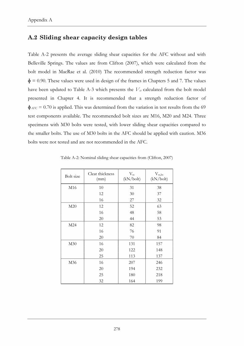
Appendix A
278
A.2 Sliding shear capacity design tables
Table A-2 presents the average sliding shear capacities for the AFC without and with
Belleville Springs. The values are from Clifton (2007), which were calculated from the
bolt model in MacRae et al. (2010) The recommended strength reduction factor was
ɸ = 0.90. These values were used in design of the frames in Chapters 5 and 7. The values
have been updated to Table A-3 which presents the Vss calculated from the bolt model
presented in Chapter 4. It is recommended that a strength reduction factor of
ɸAFC = 0.70 is applied. This was determined from the variation in test results from the 69
test components available. The recommended bolt sizes are M16, M20 and M24. Three
specimens with M30 bolts were tested, with lower sliding shear capacities compared to
the smaller bolts. The use of M30 bolts in the AFC should be applied with caution. M36
bolts were not tested and are not recommended in the AFC.
Table A-2: Nominal sliding shear capacities from (Clifton, 2007)
Bolt size Cleat thickness
(mm) Vss
(kN/bolt) Vss,bs
(kN/bolt)
M16 10 31 38
12 30 37
16 27 32
M20 12 52 63
16 48 58
20 44 53
M24 12 82 98
16 76 91
20 70 84
M30 16 131 157
20 122 148
25 113 137
M36 16 207 246
20 194 232
25 180 218
32 164 199

A.2 Sliding shear capacity tables
279
Table A-3: Revised nominal sliding shear capacities from Chapter 4
Bolt size Cleat thickness
(mm) Vss
(kN/bolt) Vss,bs
(kN/bolt)
M16 12 50 59
16 46 54
20 42 50
M20 12 86 102
16 79 94
20 74 88
M24 12 117 137
16 108 128
20 101 120
M30* 20 177 209
25 165 195
* Note that the M30 tests results were less reliable than the smaller bolts, with lower sliding shear capacities.

Appendix A
280
A.3 References
Clifton, G. C. (2007). Sliding Hinge Joint: Revisions to the Design Procedure. Heavy
Engineering Research Association, Auckland.
MacRae, G. A., Clifton, C., MacKinven, H., Mago, N., Butterworth, J. and Pampanin, S.
(2010)."The Sliding Hinge Joint moment connection." Bulletin of the New Zealand
Society for Earthquake Engineering, 43(3): 202-212.

281
Appendix B
B. Full scale subassembly tests
details
Appendix B provides details and figures from the large-scale SHJ subassembly tests that
were not presented in Chapter 6 due to length requirements of the journal. The details
provided include figures from the test setup, ring spring cartridge and testing process.
The results include the load deformation test results of the ring spring cartridges and
results from Test 8.

Appendix B
282
B.1 Test setup figures
Figure B-1 shows the fully installed SHJ on the south side before the floor deck was
installed. The four holes in the beam web as well as the extra stiffener in the column web
(between the top and bottom continuity plates) are not part of the standard SHJ or
SCSHJ configurations. Their purpose was to allow shape memory alloy (SMA) springs to
be tested as an alternative to ring springs. This was eventually not carried out due to
difficulties in machining (threading) of the bars as described in Chapter 6. Figure B-2
shows the overall test setup without the floor slab and actuator. Figure B-3 shows the
test rig during the installation of the steel deck. Figures B-4 and B-5 show the floor slab
prior and after the pouring of the concrete respectively. Figure B-6 presents the overall
test setup with installed actuator and concrete floor slab. Note that the props at the four
corners of the slab were removed before testing commenced.
Figure B-1: South side SHJ

B.1 Test setup figures
283
Figure B-2: Test setup prior to installation of floor slab
Figure B-3: Partway through installation of steel deck

Appendix B
284
Figure B-4: Test setup with deck and reinforcing mesh
Figure B-5: Concrete slab at the column slab base prior to testing

B.1 Test setup figures
285
Figure B-6: Test setup

Appendix B
286
B.2 Ring spring cartridge figures
This section illustrates the ring spring cartridge assembling process described in Section
6.3.2 with figures. Figure B-7 shows the Type 08000 ring spring cartridge, consisting of
the cage and cover plate. The ring spring (endplates on each end) is inserted into the cage
as shown in Figure B-8. The ring spring is then compressed till the length is shorter than
the cage length. The cover plate is then bolted with four M16 bolts before the tension in
the ring spring is released. Figure B-9 shows the fully assembled Type 08000 cartridge
(including the threaded bar and nuts tightened at both ends). In practice, the cartridge
was first bolted onto the bottom flange of the beam, then the threaded bar was inserted
through the centre of the cartridge and the nuts tightened. The cartridges were bolted to
the beams with four fully tensioned M16 bolts to prevent slippage between the
cartridge/flange interfaces during inelastic rotation. The typical SCSHJ with the cartridge
is shown in Figure B-10. The connection between the threaded bar and the cartridge and
column flange is shown in Figures B-11 and B-12 respectively.
Figure B-7: Unassembled Type 08000 ring spring cartridge consisting of the cage and cover plate

B.2 Ring spring cartridge figures
287
Figure B-8: Type 08000 ring spring cartridges with uncompressed ring springs
Figure B-9: Assembled Type 08000 ring spring cartridge
Figure B-10: Fully installed SCSHJ with ring spring cartridge bolted to bottom flange of beam

Appendix B
288
Figure B-11: Nut tightened at the end of the ring spring cartridge
Figure B-12: Nuts tightened on both sides of the column flange

B.3 Ring spring cartridge force-displacement behaviour
289
B.3 Ring spring cartridge force-displacement behaviour
The four ring spring cartridges, two of each Type 08000 and Type 12400 ring springs,
were tested with a load cell, LVDT and post-tensioning jack to determine their force-
displacement characteristics. They each were subjected to an arbitrary displacement
regime to verify the theoretical pre-compression force and spring stiffness calculated
from the equations in the manufacturer’s manual (Ringfeder Gmbh, 2008). The measured
results compared to the theoretical behaviours for the Type 08000 and Type 12400 ring
spring cartridges are presented in Figures B-13 and B-14 respectively.
Figure B-13: Force displacement behaviour of the Type 08000 ring spring cartridges
Figure B-14: Force displacement behaviour of the Type 12400 ring spring cartridges
ks,the = 0.92 kN/mm
0
10
20
30
40
50
60
70
80
90
0 5 10 15 20 25 30
Fo
rce
(kN
)
Displacement (mm)
Type 08000 - 1 Type 08000 - 2 Theoretical
ks,the = 1.92 kN/mm
0
20
40
60
80
100
120
140
160
180
0 2 4 6 8 10 12 14
Fo
rce
(kN
)
Displacement (mm)
Type 12400 - 1 Type 12400 - 2 Theoretical

Appendix B
290
B.4 Instrumentation
The instrumentation of the test specimen with displacement gauges is shown in Figures
B-15 and B-16. Note that two measurements were taken for gauges 1 – 2, 5 – 13 and 17
(ie. on either side of the connection). The description of each gauge is summarised in
Table B-1. The load applied by the actuator was measured through an internal load cell in
the actuator. Figure B-17 shows a figure of the instrumented panel zone.
Figure B-15: Instrumentation of the connections
17 17
1514
Load cell
Rigid
structure
16
13 13
Figure B-16: Instrumentation of the test setup
1 122
4
3
55
8
6 7
9
10
11
12

B.4 Instrumentation
291
Table B-1: Displacement gauge description
Gauge number Description
1 Displacement of the beam bottom flange relative to the column. Measured overall joint rotation
2 Slip between the bottom flange plate and beam flange. Measured AFC slip and joint inelastic rotation
3 & 4 Displacement of the web plate and the web cap plate relative to the beam web
5 Displacement between column and the top flange of the beam
6 - 12 Deformation of the panel zone, continuity plates and stiffeners. It was shown to remain elastic throughout the duration of all tests
13 Relative displacement of the threaded bar and ring spring cartridge. Measured ring spring deformation.
14 & 15 Column drift. Gauge 15 was an internal LVDT in the actuator, while Gauge 14 provided an independent measurement.
16 Slip between column base and strong floor.
17 Deformation of the rigid link.
Figure B-17: Instrumented panel zone

Appendix B
292
B.5 Test figures
Figure B-18 shows the test specimen under a drift of approximately 3%. Figure B-19
illustrates the deformation of the ring spring cartridge, where the marks on the nut
indicate the two points between maximum positive and negative deformation.
Figures B-20 and B-21 shows the force-drift and moment-rotational behaviours of
Test 8, which was the test with only the Type 08000 cartridge. Figure B-21 also presents
the comparison of the experimental response with the modified model.
Figure B-18: Deformation of assembly at 3% drift

B.5 Test figures
293
Figure B-19: Ring spring deformation
Figure B-20: Force-drift behaviour of Test 8
Figure B-21: Comparison of the joint moment-rotational behaviour in Test 8 with the modified
model
-100
-80
-60
-40
-20
0
20
40
60
80
100
-4 -3 -2 -1 0 1 2 3 4
Fo
rce
(kN
)
Drift (%)
-150
-100
-50
0
50
100
150
-35 -30 -25 -20 -15 -10 -5 0 5 10 15 20 25 30 35
Mom
ent
(kN
m)
Rotation (mrad)
Experimental
Modified IHYST 18
model

B.6 References
294
B.6 References
Ringfeder Gmbh (2008). Damping Technology. Catalogue R60. Krefeld, Germany.

295
Appendix C
C. Supplementary information for
time-history analyses
(Chapters 5 and 7)
Appendix C provides supplementary information on the analytical studies presented in
Chapters 5 to 7. The input parameters into RUAUMOKO (Carr, 2007) for the
comparison of the model and the experimental results are provided in Table C-1. No
input values to model degrading strength were used as the AFCs in the connections were
not subjected to rotations where the bolts hit the end of the slotted holes in the
experimental tests. Figures C-1 and C-2 present the response spectra of the ground
motions used for the time history analyses on the 10-storey and 5-storey frames
respectively. The input control parameters which were used in the analyses of both
frames are shown in Table C-2. An example of the input file for RUAUMOKO (Frame
B) is provided in Table C-3. Refer to Figure 7.13 for the layout of the frame, Figure 7.15
for types of connections and distribution, and Table 7.2 for details of the connection
designs. Note that the descriptions in blue fonts are not part of the model code, but were
inserted to assist in understanding of the code. Some input parameter descriptions for
“frames” modelling columns and beams, and “springs” modelling panel zones and
connections are provided in Table C-4. This is meant to aid understanding and is not an
exhaustive description. Further references should be made to the RUAUMOKO user
manual (Carr, 2007).

Appendix C
296
Table C-1: RUAUMOKO input parameters for comparison with full scale joint test results
Test Input Description
Test1 IHYST = 42 GJ = 227942 RT = 0.007 MZ+ = 123 MZ- = -123 Cspp = 1.45 Cspp = -1.45 Ru = 1 Tdp = 0.03 Tdn = -0.03 Ispr = 0
SHJ hysteretic model Rotational stiffness of the member section Bi-linear factor, or Ramberg-Osgood r, rotation Positive torsion yield Negative torsion yield Positive moment intercept Negative moment intercept Unloading stiffness factor Positive design theta Negative design theta Without Belleville Springs
AFC contribution in Test 6
IHYST = 42 GJ = 227942 RT = 0.007 MZ+ = 76.6 MZ- = -76.6 Cspp = 1.45 Cspp = -1.45 Ru = 1 Tdp = 0.03 Tdn = -0.03 Ispr = 0
SHJ hysteretic model Rotational stiffness of the member section Bi-linear factor, or Ramberg-Osgood r, rotation Positive torsion yield Negative torsion yield Positive moment intercept Negative moment intercept Unloading stiffness factor Positive design theta Negative design theta Without Belleville Springs
Test 8 and Ring spring contribution in Test 6
IHYST = 18 GJ = 42147 RT = 0.0538 MZ+ = 63.3 MZ- = -63.3 RSTEEP = 1 RLOWER = 0.0090761 DXINIT = 0.03184 KTYPE = 1 KLOOP = 1
Ring spring hysteresis Rotational stiffness of the member section Bi-linear factor, or Ramberg-Osgood r, rotation Positive torsion yield Negative torsion yield Unloading steep stiffness factor Unloading lower stiffness factor Initial displacement Bi-directional Original definition
Test 9 IHYST = 18 GJ = 20051 RT = 0.04574359 MZ+ = 30.1 MZ- = -30.1 RSTEEP = 1 RLOWER = 0.0091487 DXINIT = 0.03158 KTYPE = 1 KLOOP = 1
Ring spring hysteresis Rotational stiffness of the member section Bi-linear factor, or Ramberg-Osgood r, rotation Positive torsion yield Negative torsion yield Unloading steep stiffness factor Unloading lower stiffness factor Initial displacement Bi-directional Original definition

Appendix C
297
Figure C-1: Response spectra of ground motions for DLE (10-storey frame on rock,
T1 = 1.76 secs, Z = 0.4)
Figure C-2: Response spectra of ground motions for DLE (5-storey on deep soil,
T1 = 1.41 secs, Z = 0.4)
0.0
0.2
0.4
0.6
0.8
1.0
1.2
1.4
1.6
1.8
2.0
0 0.5 1 1.5 2 2.5 3 3.5 4 4.5 5
Acc
eler
atio
n (
×g)
Period (s)
Arcelik H1 Arcelik H2
Caleta H1 Caleta H2
Duzce H1 Duzce H2
El Centro 1940 H1 El Centro 1940 H2
El Centro 1979 #6 H1 El Centro 1979 #6 H2
Hokkaido H1 Hokkaido H2
La Union H1 La Union H2
Tabas H1 Tabas H2
TCU H1 TCU H2
Yarimka H1 Yarimka H2
Target Spectra
T1 = 1.76 1.3T1
0.4T1
0.0
0.2
0.4
0.6
0.8
1.0
1.2
1.4
1.6
1.8
2.0
0 0.5 1 1.5 2 2.5 3 3.5 4 4.5 5
Acc
eler
atio
n (
×g)
Period (s)
Caleta H1 Caleta H2
Duzce H1 Duzce H2
El Centro 1940 H1 El Centro 1940 H2
El Centro 1979 #6 H1 El Centro 1979 #6 H2
Hokkaido H1 Hokkaido H2
TCU H1 TCU H2
Yarimka H1 Yarimka H2
Target SpectraT1 = 1.41
1.3T1
0.4T1

Appendix C
298
Table C-2: Input control parameters for time-history analysis in RUAUMOKO.
Input* Description
Principal analysis options
IPANAL = 2 IFMT = 0 IPLAS = 1 IPCONM = 1 ICTYPE = 1 IPVERT = 0 INLGEO = 1 IPNF = 0 IZERO = 0 ORTHO = 0 IMODE = 1
Dynamic time-history using Newmark constant average acceleration Binary post-processor file with extension .RES In-elastic time-history analysis Diagonal mass matrix used in time-history Tangent stiffness Rayleigh damping X-direction earthquake only Large displacement effects included Modal analysis is carried out after the static analysis All zero output is omitted Mode shape orthogonality check not carried out Jacobi eigenvalue algorithm used
Frame control parameters
NNP = 320 (112) NMEM = 545 (149) NTYPE = 105 (37) M = 7 (5) MODE1 = 1 MODE2 = 10 (3) GRAV = 9.81 MODE1 = 5 MODE2 = 5 DT < 0.01 TIME FACTOR
Number of nodal points Number of members in the structure Number of different cross-section in the section table Number of mode-shapes required to be printed in the modal analysis The mode number at which the first daping ratio is applied The mode number at which the second damping ratio is applied The acceleration of gravity The percentage of critical damping at MODE1 The percentage of critical damping at MODE2 The time-step (minimum of 0.01 or time-step in time-history input) The length of time-history to be run A scale factor applied to the time-history input
Output intervals and plotting control parameters
KP = 0 KPA = 4 KPLOT = 20 DFACT = 10 XMAX = 1 YMAX = 1 NLEVEL = 11 (6) NUP = 2 IRESD = 0 KDUMP = 0
Time-history output surpressed Post-processor DYNAPLOT output every 4 time-steps Plastic hinges plotted every 20 time-steps Displacement multiplying scale factor for on-screen graphics Maximum X displacement for on-screen graphics Maximum Y displacement for on-screen graphics Number of levels computed inter-storey drifts Vertical axis for storey drifts is Y-axis Residual displacements and forces not output Maxx and stiffness matrices output supressed
Iteration control and wave velocities
MAXIT = 3 MAXCIT = 3 FTEST = 0.001 WAVEX = 0 WAVEY = 0
Maximum number of cycles of Newton-Raphson iteration per time-step Maximum number of cycles of iteration/solution step for damping models Tolerance of 10% in the residual vector Infinite wave velocity of propagation in the x-direction Infinite wave velocity of propagation in the y-direction
* Values for 10-storey frame (brackets for the 5-storey frame)

Appendix C
299
Table C-3: Example of RUAUMOKO input file (Frame B)
Input control parameters (refer to Table C-2) IPANAL
2 IFMT
0 IPLAS
1 IPCONM
1 ICTYPE
1 IPVERT
0 INGLEO
1 IPNF
0 IZERO
0 ORTHO
0 IMODE
1
NNP 112
NMEM 149
NTYPE 37
M 5
MODE1 1
MODE2 3
GRAV 9.81
C1 5
C2 5
DT 0.002
TIME 10
FACTOR 1.09
KP 0
KPA 4
KPLOT 20
JOUT 0
DSTORT 1
DFACT 10
XMAX 0.7
YMAX 0.1
MAXIT 3
MAXCIT 3
FTEST 0.001
WAVEX 0
WAVEY 0
Nodes 1 * Defining position of nodes* N
1 X(N)
0 Y(N)
0 NF1
1 NF2
1 NF3
1 KUP1
0 KUP2
0 KUP3
0 2 0 0 0 0 0 1 1 1 N Nodal number
3 7 0 1 1 1 0 0 0 X(N) X-coordinate
4 7 0 0 0 0 3 3 3 Y(N) Y-coordinate
5 14 0 1 1 1 0 0 0 NF1 X, Y, Z displacement constrained (0) or fixed (1)
6 14 0 0 0 0 5 5 5 NF2
7 21 0 1 1 1 0 0 0 NF3
8 21 0 0 0 0 7 7 7 KUP1 X,Y, Z displacement no coupling (0) or coupled to node
9 0 3.5 0 0 0 15 0 0 KUP2
10 0 3.5 0 0 0 15 9 0 KUP3
11 0.33 3.5 0 0 0 0 0 0 12 0.33 3.5 0 0 0 11 11 0 13 6.67 3.5 0 0 0 14 14 0 14 6.67 3.5 0 0 0 0 0 0 15 7 3.5 0 0 0 0 0 0 16 7 3.5 0 0 0 15 15 0 17 7.33 3.5 0 0 0 0 0 0 18 7.33 3.5 0 0 0 17 17 0 19 13.67 3.5 0 0 0 20 20 0 20 13.67 3.5 0 0 0 0 0 0 21 14 3.5 0 0 0 15 0 0 22 14 3.5 0 0 0 15 21 0 23 14.33 3.5 0 0 0 0 0 0 24 14.33 3.5 0 0 0 23 23 0 25 20.67 3.5 0 0 0 26 26 0 26 20.67 3.5 0 0 0 0 0 0 27 21 3.5 0 0 0 15 0 0 28 21 3.5 0 0 0 15 27 0 29 0 7 0 0 0 35 0 0 30 0 7 0 0 0 35 29 0 31 0.33 7 0 0 0 0 0 0 32 0.33 7 0 0 0 31 31 0 33 6.67 7 0 0 0 34 34 0 34 6.67 7 0 0 0 0 0 0 35 7 7 0 0 0 0 0 0 36 7 7 0 0 0 35 35 0 37 7.33 7 0 0 0 0 0 0 38 7.33 7 0 0 0 37 37 0 39 13.67 7 0 0 0 40 40 0 40 13.67 7 0 0 0 0 0 0 41 14 7 0 0 0 35 0 0 42 14 7 0 0 0 35 41 0 43 14.33 7 0 0 0 0 0 0 44 14.33 7 0 0 0 43 43 0 45 20.67 7 0 0 0 46 46 0 46 20.67 7 0 0 0 0 0 0 47 21 7 0 0 0 35 0 0 48 21 7 0 0 0 35 47 0 49 0 8.5 0 0 0 0 0 0 50 7 8.5 0 0 0 0 0 0 51 14 8.5 0 0 0 0 0 0 52 21 8.5 0 0 0 0 0 0 53 0 10.5 0 0 0 59 0 0 54 0 10.5 0 0 0 59 53 0 55 0.33 10.5 0 0 0 0 0 0 56 0.33 10.5 0 0 0 55 55 0 57 6.67 10.5 0 0 0 58 58 0 58 6.67 10.5 0 0 0 0 0 0 59 7 10.5 0 0 0 0 0 0 60 7 10.5 0 0 0 59 59 0 61 7.33 10.5 0 0 0 0 0 0 62 7.33 10.5 0 0 0 61 61 0 63 13.67 10.5 0 0 0 64 64 0 64 13.67 10.5 0 0 0 0 0 0 65 14 10.5 0 0 0 59 0 0

Appendix C
300
66 14 10.5 0 0 0 59 65 0 67 14.33 10.5 0 0 0 0 0 0 68 14.33 10.5 0 0 0 67 67 0 69 20.67 10.5 0 0 0 70 70 0 70 20.67 10.5 0 0 0 0 0 0
71 21 10.5 0 0 0 59 0 0 72 21 10.5 0 0 0 59 71 0 73 0 14 0 0 0 79 0 0 74 0 14 0 0 0 79 73 0 75 0.31 14 0 0 0 0 0 0 76 0.31 14 0 0 0 75 75 0 77 6.69 14 0 0 0 78 78 0 78 6.69 14 0 0 0 0 0 0 79 7 14 0 0 0 0 0 0 80 7 14 0 0 0 79 79 0 81 7.31 14 0 0 0 0 0 0 82 7.31 14 0 0 0 81 81 0 83 13.69 14 0 0 0 84 84 0 84 13.69 14 0 0 0 0 0 0 85 14 14 0 0 0 79 0 0 86 14 14 0 0 0 79 85 0 87 14.31 14 0 0 0 0 0 0 88 14.31 14 0 0 0 87 87 0 89 20.69 14 0 0 0 90 90 0 90 20.69 14 0 0 0 0 0 0 91 21 14 0 0 0 79 0 0 92 21 14 0 0 0 79 91 0 93 0 17.5 0 0 0 99 0 0 94 0 17.5 0 0 0 99 93 0 95 0.30 17.5 0 0 0 0 0 0 96 0.30 17.5 0 0 0 95 95 0 97 6.70 17.5 0 0 0 98 98 0 98 6.70 17.5 0 0 0 0 0 0 99 7 17.5 0 0 0 0 0 0 100 7 17.5 0 0 0 99 99 0 101 7.30 17.5 0 0 0 0 0 0 102 7.30 17.5 0 0 0 101 101 0 103 13.70 17.5 0 0 0 104 104 0 104 13.70 17.5 0 0 0 0 0 0 105 14 17.5 0 0 0 99 0 0 106 14 17.5 0 0 0 99 105 0 107 14.30 17.5 0 0 0 0 0 0 108 14.30 17.5 0 0 0 107 107 0 109 20.70 17.5 0 0 0 110 110 0 110 20.70 17.5 0 0 0 0 0 0 111 21 17.5 0 0 0 99 0 0 112 21 17.5 0 0 0 99 111 0 Elements 1 * Defining elements from props and locations in frame* N
1 MT 1
NODE1 2
NODE2 9
2 2 9 10 3 3 9 29
N Element number 4 4 29 30
MT Member type (from Props below)
5 5 29 49
NODE1 Nodal number at end 1 of the member 6 6 53 54
NODE2 Nodal number at end 2 of the member
7 7 53 73 8 8 73 74 9 9 73 93 10 10 93 94 11 11 10 11 12 11 30 31 13 11 54 55 14 11 74 75 15 11 94 95 16 12 11 12 17 13 11 12 18 14 31 32 19 15 31 32 20 16 55 56 21 17 55 56 22 18 75 76 23 19 75 76 24 20 95 96 25 21 95 96 26 22 12 13 27 23 32 33 28 24 56 57 29 25 76 77 30 26 96 97

Appendix C
301
31 28 13 14 32 29 13 14 33 30 33 34 34 31 33 34 35 32 57 58 36 33 57 58 37 34 77 78 38 35 77 78 39 36 97 98 40 37 97 98 41 11 14 16 42 11 34 36 43 11 58 60 44 11 78 80 45 11 98 100 46 1 4 15 47 2 15 16 48 3 15 35 49 4 35 36 50 5 35 50 51 6 59 60 52 7 59 79 53 8 79 80 54 9 79 99 55 10 99 100 56 11 16 17 57 11 36 37 58 11 60 61 59 11 80 81 60 11 100 101 61 28 17 18 62 29 17 18 63 30 37 38 64 31 37 38 65 32 61 62 66 33 61 62 67 34 81 82 68 35 81 82 69 36 101 102 70 37 101 102 71 22 18 19 72 23 38 39 73 24 62 63 74 25 82 83 75 26 102 103 76 28 19 20 77 29 19 20 78 30 39 40 79 31 39 40 80 32 63 64 81 33 63 64 82 34 83 84 83 35 83 84 84 36 103 104 85 37 103 104 86 11 20 22 87 11 40 42 88 11 64 66 89 11 84 86 90 11 104 106 91 1 6 21 92 2 21 22 93 3 21 41 94 4 41 42 95 5 41 51 96 6 65 66 97 7 65 85 98 8 85 86 99 9 85 105 100 10 105 106 101 11 22 23 102 11 42 43 103 11 66 67 104 11 86 87 105 11 106 107 106 28 23 24 107 29 23 24 108 30 43 44 109 31 43 44

Appendix C
302
110 32 67 68 111 33 67 68 112 34 87 88 113 35 87 88 114 36 107 108 115 37 107 108 116 22 24 25 117 23 44 45 118 24 68 69 119 25 88 89 120 26 108 109 121 12 25 26 122 13 25 26 123 14 45 46 124 15 45 46 125 16 69 70 126 17 69 70 127 18 89 90 128 19 89 90 129 20 109 110 130 21 109 110 131 11 26 28 132 11 46 48 133 11 70 72 134 11 90 92 135 11 110 112 136 1 8 27 137 2 27 28 138 3 27 47 139 4 47 48 140 5 47 52 141 6 71 72 142 7 71 91 143 8 91 92 144 9 91 111 145 10 111 112 146 27 49 53 147 27 50 59 148 27 51 65 149 27 52 71 Props * Defining properties of props, see Table C-1 and C-4*
1 frame *Columns* ITYPE
3 IPIN
0 ICOND
0 IHYST
2 ILOS
0 IDAMG
1 ICOL
0 E
205000000 G
80000000 A
0.047 AS
0.015 I
0.004 WGT 3.65
END1 0
END2 0.312
FJ1 1.38E-05
FJ2 0
RA 0
RF 0.03
H1 0
H2 0
PYC -14259.6
PB -2181.7
MB 3664.9
M0 3664.9
PC 2181.7
MC 3664.9
PYT 14259.6
MUT 2
MUC 2
MU1+ 4
MU2+ 4
MU2+ 4
MU2- 4
2 spring *Panel zone* ITYPE
1 IHYST
2 ILOSE
0 IDAMG
1 KX 0
KY 0
G 651154.4
WGT 0
RF 0.03
RT 0.05
FX+ 0
FX- 0
FY+ 0
FY- 0
MZ+ 2165.9
MZ- -2165.9
MUX+ 1
MUX- 1
MUY+ 1
MUY- 1
MUR+ 10
MUR- 10
3 frame 3 0 0 2 0 1 0 205000000 80000000 0.039 0.013 0.003 3.01 0.312 0.309 0 0 0 0.03 0 0 -12228.7 -1871.0 3101.5 3664.9 1871.0 3101.5 12228.7
2 2 4 4 4 4 4 spring 1 2 0 1 0 0 651154.4 0 0.03 0.05 0 0 0 0 2165.9 -2165.9 1 1 1 1 10 10 5 frame 3 0 0 2 0 1 0 205000000 80000000 0.039 0.013 0.003 3.01 0.309 0 0 0 0 0.03 0 0 -12228.7 -1871.0 3101.5 3101.5 1871.0 3101.5 12228.7 0 2 2 4 4 4 4 6 spring 1 2 0 1 0 0 528523.2 0 0.03 0.05 0 0 0 0 2165.9 -2165.9 1 1 1 1 10 10 7 frame 3 0 0 2 0 1 0 205000000 80000000 0.022 0.009 0.001 1.68 0.306 0.301 0 0

Appendix C
303
0 0.03 0 0 -6826.7 -1044.5 1614.4 3664.9 1044.5 1614.4 6826.7 0 2 2 4 4 4 4 8 spring 1 2 0 1 0 0 341689.9 0 0.03 0.05 0 0 0 0 1411.1 -1411.1 1 1 1 1 10 10 9 frame 3 0 0 2 0 1 0 205000000 80000000 0.010 0.006 0.001 0.80 0.301 0.264 0 0 0 0.03 0 0 -2911.4 -445.4 711.7 3664.9 516.9 711.7 3378.4 0 2 2 4 4 4 4 10 spring 1 2 0 1 0 0 293801.6 0 0.03 0.05 0 0 0 0 1041.0 -1041.0 1 1 1 1 10 10 11 frame 1 0 0 0 0 0 205000000 80000000 1 0 1 0 0 0 0 0 12 spring *Sliding Hinge Joint, see Table C-1* ITYPE
1 IHYST
42 ILOS
1 IDAMG
0 KX 0
KY 0
GJ 322453.6
WGT 0
RF 1
RT 0.007
FX+ 0
FX- 0
FY+ 0
FY- 0
MZ+ 721.9
MZ- -721.9
DUCT1 27.14
DUCT2 29.28
RDUCT 0.60
DUCT3 37.84
Cspp 1.45
Cspn 1.45
Ru 1.00
Tdp 0.030
Tdn -0.030
Ispr 0.00
1.45 1.45 1.00 0.030 -0.030 0.00
13 spring *Ring spring component, see Table C-1* ITYPE
1 IHYST
18 ILOS
0 IDAMG
0 KX 0
KY 0
GJ 191405.0
WGT 0
RF 1
RT 0.02403
RSTEEP 1
RLOWER 0.00480552
DXINIT 0.0655031
KTYPE 1
KLOOP 1
14 spring
1 42 1 0 0 0 289058.1 0 1 0.007
0 0 0 0 647.1 -647.1
27.16 29.32 0.60 37.96
1.45 1.45 1.00 0.030 -0.030 0.00
1.45 1.45 1.00 0.030 -0.030 0.00
15 spring
1 18 0 0 0 0 173096.8 0 1 0.02599
1 0.00519833 0.0610333 1 1
16 spring
1 42 1 0 0 0 243785.3 0 1 0.007
0 0 0 0 545.8 -545.8
27.18 29.36 0.60 38.07
1.45 1.45 1.00 0.030 -0.030 0.00
1.45 1.45 1.00 0.030 -0.030 0.00
17 spring
1 18 0 0 0 0 109395.0 0 1 0.02954
1 0.00590857 0.0539943 1 1
18 spring
1 42 1 0 0 0 135173.6 0 1 0.007
0 0 0 0 302.6 -302.6
27.21 29.43 0.60 38.29
1.45 1.45 1.00 0.030 -0.030 0.00
1.45 1.45 1.00 0.030 -0.030 0.00
19 spring
1 18 0 0 0 0 67499.3 0 1 0.03206
1 0.00641219 0.0504741 1 1
20 spring
1 42 1 0 0 0 59089.5 0 1 0.007
0 0 0 0 132.3 -132.3
27.53 30.05 0.60 40.15
1.45 1.45 1.00 0.03 -0.03 0.00
1.45 1.45 1.00 0.03 -0.03 0.00
21 spring
1 18 0 0 0 0 0.0 0 1 0.00100
1 0.0002 1.8924239 1 1
22 frame *Beam* ITYPE
1 IPIN
0 ICOND
1 IHYST
0 ILOS
0 IDAMG
0 E
205000000 G
80000000 A
0.020 AS
0.008 I
0.002 WGT
0 END1
0 END2
0 FJ1 0
FJ2 0
M1 -103
M2 -103
V1 -118
V2 118
AXIAL 0
AXPS 0
23 frame
1 0 1 0 0 0
205000000 80000000 0.018 0.007 0.001 0 0 0 0 0
-103 -103 -118 118 0 0
24 frame

Appendix C
304
1 0 1 0 0 0
205000000 80000000 0.016 0.007 0.001 0 0 0 0 0
-103 -103 -118 118 0 0
25 frame
1 0 1 0 0 0
205000000 80000000 0.013 0.006 0.001 0 0 0 0 0
-103 -103 -118 118 0 0
26 frame
1 0 1 0 0 0
205000000 80000000 0.011 0.005 0.001 0 0 0 0 0
-46.5 -46.5 -53.6 53.6 0 0
27 frame
3 0 0 2 0 1 0
205000000 80000000 0.034 0.014 0.002 2.65 0 0.306 0 0
0 0.03 0 0
-10309.1 -1577.3 2495.1 3664.9 1577.3 2495.1 10309.1 0
2 2 4 4 4 4
28 spring
1 42 1 0 0 0 322453.6 0 1 0.007
0 0 0 0 721.9 -721.9
27.14 29.28 0.60 37.84
1.45 1.45 1.00 0.030 -0.030 0.00
1.45 1.45 1.00 0.030 -0.030 0.00
29 spring
1 18 0 0 0 0 191405.0 0 1 0.02
1 0.00322731 0.0981681 1 1
30 spring
1 42 1 0 0 0 289058.1 0 1 0.007
0 0 0 0 647.1 -647.1
27.16 29.32 0.60 37.96
1.45 1.45 1.00 0.030 -0.030 0.00
1.45 1.45 1.00 0.030 -0.030 0.00
31 spring
1 18 0 0 0 0 173096.8 0 1 0.02
1 0.00342028 0.0934413 1 1
32 spring
1 42 1 0 0 0 243785.3 0 1 0.007
0 0 0 0 545.8 -545.8
27.18 29.36 0.60 38.07
1.45 1.45 1.00 0.030 -0.030 0.00
1.45 1.45 1.00 0.030 -0.030 0.00
33 spring
1 18 0 0 0 0 109395.0 0 1 0.02
1 0.00396885 0.0810282 1 1
34 spring
1 42 1 0 0 0 135173.6 0 1 0.007
0 0 0 0 302.6 -302.6
27.21 29.43 0.60 38.29
1.45 1.45 1.00 0.030 -0.030 0.00
1.45 1.45 1.00 0.030 -0.030 0.00
35 spring
1 18 0 0 0 0 67499.3 0 1 0.02
1 0.00425217 0.0767963 1 1
36 spring
1 42 1 0 0 0 59089.5 0 1 0.007
0 0 0 0 132.3 -132.3
27.53 30.05 0.60 40.15
1.45 1.45 1.00 0.03 -0.03 0.00
1.45 1.45 1.00 0.03 -0.03 0.00
37 spring
1 18 0 0 0 0 0.0 0 1 0.00
1 0.0002 1.8924239 1 1
weight 0 *Defining weights* N
1 WX
0 WY
0 9 532.5 532.5 N Nodal point number
15 532.5 532.5 WX Lumped nodal weight in X direction 21 532.5 532.5 WY Lumped nodal weight in Y direction 27 532.5 532.5
29 532.5 532.5 35 532.5 532.5 41 532.5 532.5 47 532.5 532.5 53 532.5 532.5 59 532.5 532.5 65 532.5 532.5 71 532.5 532.5 73 532.5 532.5 79 532.5 532.5

Appendix C
305
85 532.5 532.5 91 532.5 532.5 93 227.5 227.5 99 227.5 227.5 105 227.5 227.5 111 227.5 227.5 112 0 0 loads * Defining loads *
N 1
FX 0
FY 0
FM 0
2 0 0 0
N Nodal point number 3 0 0 0
FX Lumped nodal weight acting in the X direction
4 0 0 0
FY Lumped nodal weight acting in the YX direction 5 0 0 0
FM Lumped nodal weight acting in rotation at the node
6 0 0 0 7 0 0 0 8 0 0 0 9 0 -100 0 10 0 0 0 11 0 0 0 12 0 0 0 13 0 0 0 14 0 0 0 15 0 18 0 16 0 0 0 17 0 0 0 18 0 0 0 19 0 0 0 20 0 0 0 21 0 18 0 22 0 0 0 23 0 0 0 24 0 0 0 25 0 0 0 26 0 0 0 27 0 -100 0 28 0 0 0 29 0 -103 0 30 0 0 0 31 0 0 0 32 0 0 0 33 0 0 0 34 0 0 0 35 0 15 0 36 0 0 0 37 0 0 0 38 0 0 0 39 0 0 0 40 0 0 0 41 0 15 0 42 0 0 0 43 0 0 0 44 0 0 0 45 0 0 0 46 0 0 0 47 0 -103 0 48 0 0 0 49 0 0 0 50 0 0 0 51 0 0 0 52 0 0 0 53 0 -103 0 54 0 0 0 55 0 0 0 56 0 0 0 57 0 0 0 58 0 0 0 59 0 15 0 60 0 0 0 61 0 0 0 62 0 0 0 63 0 0 0 64 0 0 0 65 0 15 0 66 0 0 0 67 0 0 0 68 0 0 0 69 0 0 0 70 0 0 0

Appendix C
306
71 0 -103 0 72 0 0 0 73 0 -118 0 74 0 0 0 75 0 0 0 76 0 0 0 77 0 0 0 78 0 0 0 79 0 0 0 80 0 0 0 81 0 0 0 82 0 0 0 83 0 0 0 84 0 0 0 85 0 0 0 86 0 0 0 87 0 0 0 88 0 0 0 89 0 0 0 90 0 0 0 91 0 -118 0 92 0 0 0 93 0 -32.4 0 94 0 0 0 95 0 0 0 96 0 0 0 97 0 0 0 98 0 0 0 99 0 21.2 0 100 0 0 0 101 0 0 0 102 0 0 0 103 0 0 0 104 0 0 0 105 0 21.2 0 106 0 0 0 107 0 0 0 108 0 0 0 109 0 0 0 110 0 0 0 111 0 -32.4 0 112 0 0 0 equake *Defining earthquake input*
IBERG 0
ISTART 1
DELTAT 0.01
ASCALE 1
END 0
VEL 0
DIS 0
TSCALE 1

Appendix C
307
Table C-4: Input element property descriptions for time-history analysis in RUAUMOKO.
Input Description
Frame
ITYPE IPIN ICOND IHYST ILOS IDAMG ICOL
Element type (eg. beam = 1, steel beam-column = 3) Member end connection (eg. built-in = 0, end 1 pinned = 1) Initial loading conditions (eg. no initial loads = 0) Hysteresis rule (eg. elastic = 0, elasto-plastic = 1) Strength degradation (eg. no strength degradation = 0) Computation of damage indices (eg. no damage indices computed = 0) Column ductilities computation (eg. computed at balance point = 0).
E G A AS I WGT END1 END2 FJ1 FJ2
Elastic Modulus of member material Shear Modulus of member material Cross-sectional area of the member section Effective shear area of the member section Moment of intertia of section Weight/(unit length) of the member Length of rigid end-block of End 1 Length of rigid end-block of End 2 Joint flexibility at End 1 Joint flexibility at End 2
M1 M2 V1 V2 AXIAL AXPS
Fixed-end moment at End 1 Fixed-end moment at End 2 Fixed-end shear force at End 1 Fixed-end shear force at End 2 Axial force applied to member Axial prestress in the member
PYC PB MB M0 PC MC PYT
Axial compression yield force Axial compression force at B (see figure) Yield moment at B (see figure) Yield moment at P = 0 (see figure) Axial tension force at C (see figure) Yield moment at C (see figure) Axial tension yield force Steel beam-column yield interaction
surface (Carr, 2007) MUT MUC MU1+ MU1- MU2+ MU2-
Positive axial ultimate ductility Negative axial ultimate ductility Positive ultimate ductility (End 1) Negative ultimate ductility (End 1) Positive ultimate ductility (End 2) Negative ultimate ductility (End 2)

Appendix C
308
Spring
ITYPE IHYST ILOS IDAMG KX KY GJ WGT RF RT FX+ FX- FY+ FY- MZ+ MZ- MUX+ MUX- MUY+ MUY- MUR+ MUR-
Interaction between X, Y or theta Z components (eg. no interaction = 0) Hysteresis rule (eg. ring spring = 18, SHJ = 42) Strength degradation (eg. strength reduction base on ductility in that direction = 1) Computation of damage indices (eg. not computed = 0) Spring stiffness in the local X-direction Spring stiffness in the local Y-direction Rotational stiffness of the member section Weight/(unit length) of the member Bi-linear factor, spring forces Bi-linear factor, rotation Positive spring yield force in the X direction Negative spring yield force in the X direction Positive spring yield force in the Y direction Negative spring yield force in the Y direction Positive torsional yield Negative torsional yield Positive ultimate ductility (X direction) Negative ultimate ductility (X direction) Positive ultimate ductility (Y direction) Negative ultimate ductility (Y direction) Positive rotational ultimate ductility Negative rotational ultimate ductility
C.1 References
Carr, A. (2007). RUAUMOKO2D. Civil Engineering Department, University of
Canterbury, Christchurch, New Zealand.
Carr, A. (2012). RUAUMOKO2D. Civil Engineering Department, University of
Canterbury, Christchurch, New Zealand (specially provided by the author for this
project).