12735 15 lec 09 8 apr - cmu12735: urban systems modeling lec. 09 bayesian networks applications 8...

Lec. 0912735: Urban Systems Modeling Bayesian Networks

12735: Urban Systems Modeling

instructor: Matteo Pozzi

1

Bayesian Networks

Lec. 09

x1

x3 x4

x2

x6

x5

x8x7

x9


outline

2

‐ example of applications

‐ how to shape a problem as a BN

‐ complexity of the inference problem

‐ inference via variable elimination

‐ inference via junction tree

‐ MCMC approximate inference


intro on Bayesian Networks

3

magnitudoseismic intensity Discrete variables, possible values for each var.

JOINT PROBABILITYChain rule (product rule)

, , ,table

damage

1table table,

table

Each variable is defined by a table withnumber of dimensions equal to number of parents plus one.

random variables are nodes,links defines conditional dependence/independence.


example of Bayesian network

4

x1

x3

scenario

x4

x2

x6

x5

x8x7

material

strength

damagedemand

stiffness

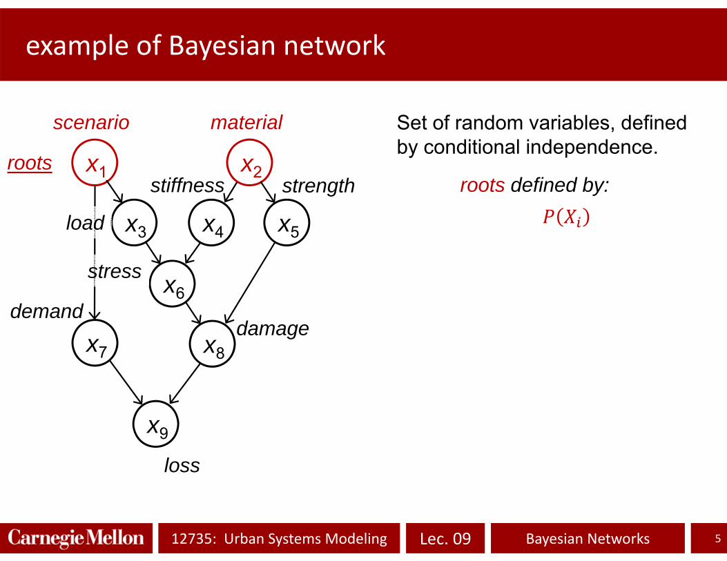
Set of random variables, defined by conditional independence.

loss

x9

load

stress



5

x1

x3

scenario

x4

x2

x6

x5

x8x7

material

strength

damagedemand

stiffness

loss

x9

load

stress

roots


roots defined by:



6

x1

x3

scenario

x4

x2

x6

x5

x8x7

material

strength

damagedemand

stiffness

loss

x9

load

stress

roots


parentschildren defined by:

parent

child

roots defined by:



7

x1

x3

scenario

x4

x2

x6

x5

x8x7

material

strength

damagedemand

stiffness

loss

x9

load

stress

roots


parent

child

roots defined by:

parents

joint probability:

task: prediction – conditional prediction

parentschildren defined by:


applications

8

‐ integrated risk analysis

‐ predicting global warming

‐ predicting effects of natural hazards

‐ road construction

‐ time models: degrading systems, e.g. due to fatigue HMM

‐ time models: vibration of structures (Kalman Filter)


example of 2 vars. BN

9

magnitudoseismic intensity Discrete variables,

possible values for each variable

Joint probability, : table: 1degreesoffreedom (dofs)

Chain rule (product rule),: 1table: 1dofs: table: dofs

,,

1

1

∀ : 1

fully connected, or complete graph

if :

, : 2 2dofs

this reduced graph is less powerful than the complete one.It can represent only joint probability satisfying . However inference is much easier for this graph:


P (Y ) Y 1 Y 2 Y 3

20% 50% 30% 100%

P (X ) P (X ,Y ) Y 1 Y 2 Y 3

X 1 10% X 1 2% 5% 3% 10%X 2 60% X 2 3% 30% 27% 60%X 3 30% X 3 15% 15% 0% 30%

100% 20% 50% 30% 100%

P (Y ) Y 1 Y 2 Y 3

20% 50% 30% 100%

P (X ) P (X ,Y ) Y 1 Y 2 Y 3

X 1 10% X 1 2% 5% 3% 10%X 2 60% X 2 12% 30% 18% 60%X 3 30% X 3 6% 15% 9% 30%

100% 20% 50% 30% 100%

Independence [from lec.2]

10

,

,

,

,the joint prob. is “richer” than the set of marginal prob.

the joint prob. is no “richer” than the set of marginal prob.

12

3

12

3

0

0.1

0.2

0.3

XY

P(X

,Y)

12

3

12

3

0

0.1

0.2

0.3

XY

P(X

,Y)


example of 3 vars. BN

11

magnitudoseismic intensity Discrete variables, possible values for each var.

Joint probability, , : table: 1dofs

Chain rule (product rule), , ,

, ,, ,

1

complete graph

if | : ,

damage

, ,1 2 2 N 1dofs

After observing intensity , any additional information on magnitudo is irrelevant for inferring the damage .conditional independence


chain graph for n vars

12

…Complete graph:

: table: 1dofs

If ∀ , … , | : , … ,

, … ,

1 1 ≅ dofs

Chain graph

1 2 3 4 5 6 7 8 9101

103

105

107

109

n

num

ber o

f dof

s

N = 10

completechain

the chain graph is less powerful, but much easier to handle.

…


prediction by variable elimination

13

M I D

magnitudoseismic intensity

damage, ,

build joint probability:

derive marginal probability by marginalization:

, ,,

table

,I D

D

we can derive without handling any 3‐d table: only handling 1‐d and 2‐d tables.

you can derive everything from the joint prob.:

vector matrix product


prediction by variable elimination [cont.]

14

M I D


damage

,I

1

M

I

, ,build joint probability:


, ,,

table



prediction by variable elimination [cont.]

15

M I D


damage

,I

1

M

1M



, ,,

table



inference by variable elimination

16

M I D


damage

,M



, , , /

table


D

,,

normalization:


inference by variable elimination [cont.]

17

M I D


damage

,



, , , /

table


D

,,

normalization:

I


best order of elimination

18

x3 x4

x6

x5

x8

strength

damage

load

stress

stiffness

, , , , ,

, ,

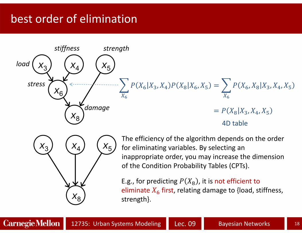
x3 x4 x5

x8

4D table

The efficiency of the algorithm depends on the order for eliminating variables. By selecting an inappropriate order, you may increase the dimension of the Condition Probability Tables (CPTs).

E.g., for predicting , it is not efficient to eliminate first, relating damage to {load, stiffness, strength}.


D1 D2 |

task: modeling

branching graph

19

D1

I

seismic intensity

damage on building 2


D2

damage on building 1

∝ ,

,

, ∝ , , ∝cost.

, 1

prediction:

after observing :

after observing and :

is irrelevant

and are NOT independent, while is not fixed.

is irrelevant after

1‐d table

3‐d table

no 3‐d table is used

D1 D2


V graph

20

L1

Ddamage

load 2, , ,


L2

load 1

L1 L2

,,

,, 1

prediction:

after observing :

task: modeling

, are irrelevant

as L1 L2

,

,

∝ , ,

, ∝

1cost.


V graph [cont.]

21

L1

Ddamage

load 2, , ,


L2

load 1

,

L1 L2

task: modeling

after observing :

knowledge on L1 is used for building likelihood .

∝ , ,

,

after observing and :

conditionally to (having observed) , variables L1 and L2 are NOT independent.

, ∝ , , , ∝ ,cost.

L1 L2 |

this is an example of INDUCED DEPENDENCE(induced correlation)


inference via variable elimination and junction tree

22

M I D


damage

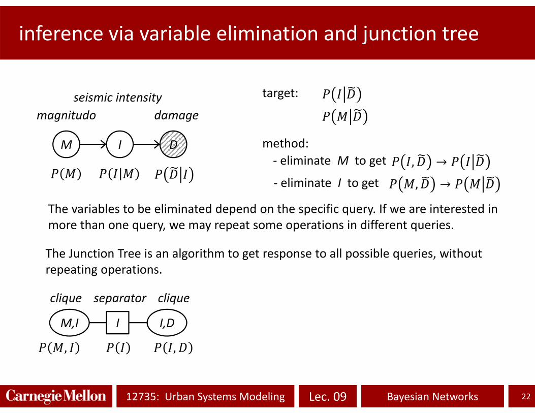
target:

M,I I,D

, →

method:

‐ eliminate I to get

, →‐ eliminate M to get

The variables to be eliminated depend on the specific query. If we are interested in more than one query, we may repeat some operations in different queries.

I

clique cliqueseparator

, ,

The Junction Tree is an algorithm to get response to all possible queries, without repeating operations.


HHM revised

23

Sk Sk+1

yk yk+1

S1

y1

Sn

yn

S0 … … task:compute

:

eliminate , process , eliminate , process , … , eliminate , process .(eliminate) (eliminate) (eliminate)

The prediction‐correction algorithm is an application of a best elimination order.


conditions for exact inference

24

‐ Discrete variables, except for “course of dimensionality”.

‐ Continuous variables: integral instead of sum. Generally integrals cannot be solved in close form. But they can be solved for Gaussian Linear Models (GLM).

x3

x4

x1

x6x2

x5, ,

condition for GLM: if vector lists all parents of :

x7

‐ Other problems can be also mapped into a GLM. For example Log‐normal models can be mapped by taking into GLMs by taking the log.

‐ Hybrid graphs have also been proposed, mixing discrete and continuous variables, by imposing some rules.

‐ GLM can be seen as a special case of Gaussian processes, with special independency relations (while Gaussian processes are complete graphs).

GLMs are used for dynamic systems (Kalman filters)


approximate inference

25

‐MC: sequential sampling. We start sampling roots from their marginal, then each other variables conditional to their (sampled) parents. After observing any variable, we can reject samples non compatible with observations, or use importance sampling.

‐MCMC: Gibbs sampling. We samples randomly variables conditional to the other vars. In the Markov blanket (kept fixed). It is an application of the Metropolis algorithm with special proposal distribution.

Markov blanket

Gibbs sampling

Russell, S. and P. Norvig. (2010). Artificial Intelligence: A Modern Approach. Pearson Education.

Barber, B. (2012). Bayesian Reasoning and Machine Learning. Cambridge UP


summary

26

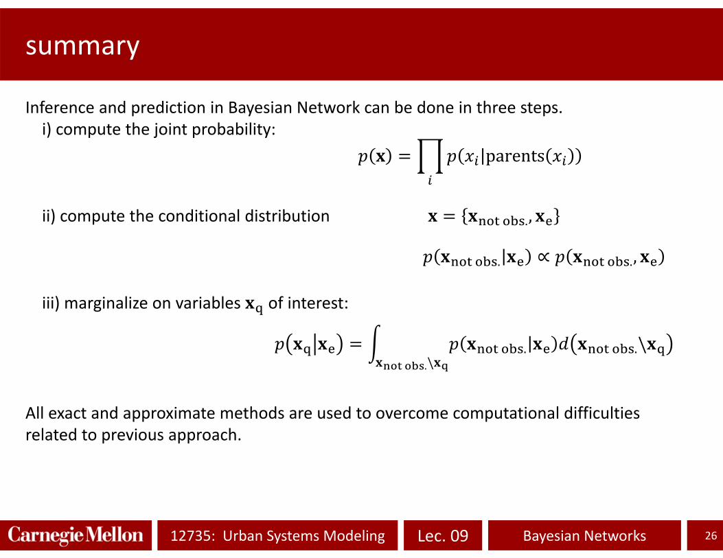
Inference and prediction in Bayesian Network can be done in three steps.i) compute the joint probability:

ii) compute the conditional distribution

iii) marginalize on variables of interest:

All exact and approximate methods are used to overcome computational difficulties related to previous approach.

parents

. ∝ .,

.,

. .\ .\


HHM with dummy algorithm

27

Sk Sk+1

yk yk+1

S1

y1

Sn

yn

S0 … … task:compute

:

i) compute the joint probability: : , : ∏

ii) compute the conditional distribution: : : ∝ : , :

iii) marginalize on variables of interest : : ∑ : ::

huge table/function:it is not an effective path


references

28

Barber, B. (2012). Bayesian Reasoning and Machine Learning. Cambridge UP. Downloadable from http://web4.cs.ucl.ac.uk/staff/D.Barber/pmwiki/pmwiki.php?n=Brml.HomePage

Bishop, C. (2006). Pattern Recognition and Machine Learning. Springer

Russell, S. and P. Norvig. (2010). Artificial Intelligence: A Modern Approach. Pearson Education.

12735 15 lec 09 8 apr - cmu12735: urban systems modeling lec. 09 bayesian networks applications 8...

Documents