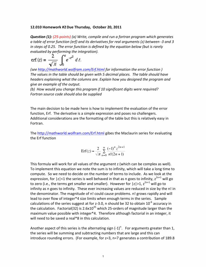
12.010  Homework  #2  Due  Thursday,    October  20,  2011   Question  (1):  (25-­‐points)  (a)  Write,  compile  and  run  a  fortran  program  which  generates  a  table  of  error  function  (erf)  and  its  derivatives  for  real  arguments  (z)  between  -­‐3  and  3  in  steps  of  0.25.    The  error  function  is  defined  by  the  equation  below  (but  is  rarely  evaluated  by  performing  the  integration).  

 (see  http://mathworld.wolfram.com/Erf.html  for  information  the  error  function  )  The  values  in  the  table  should  be  given  with  5  decimal  places.    The  table  should  have  headers  explaining  what  the  columns  are.  Explain  how  you  designed  the  program  and  give  an  example  of  the  output.  (b)    How  would  you  change  this  program  if  10  significant  digits  were  required?      Fortran  source  code  should  also  be  supplied   The  main  decision  to  be  made  here  is  how  to  implement  the  evaluation  of  the  error  function,  Erf.    The  derivative  is  a  simple  expression  and  poses  no  challengers.      Additional  considerations  are  the  formatting  of  the  table  but  this  is  relatively  easy  in  Fortran.    The  http://mathworld.wolfram.com/Erf.html  gibes  the  Maclaurin  series  for  evaluating  the  Erf  function    

2 (Erf(z)$ #1)n z2n+1  

= %" n=0 n!(2n +1)

 This  formula  will  work  for  all  values  of  the  argument  z  (which  can  be  complex  as  well).    To  implement  this  equation  we  note  the  sum  is  to  infinity,  which  will  take  a  long  time  to  compute.    So  we  need  to  decide  on  the  number  of  terms  to  include.    As  we  look  at  the  expression,  for  |z|<1  the  series  is  well  behaved  in  that  as  n  goes  to  infinity,  z2n+1  will  go  to  zero  (i.e.,  the  terms  get  smaller  and  smaller).    However  for  |z|>1,  z2n+1  will  go  to  infinity  as  n  goes  to  infinity.    These  ever  increasing  values  are  reduced  in  size  by  the  n!  in  the  denominator.  The  magnitude  of  n!  could  cause  problems.  n!  grows  rapidly  and  will  lead  to  over  flow  of  integer*4  size  limits  when  enough  terms  in  the  series.      Sample  calculations  of  the  series  suggest  at  for  z-­‐3.0,  n  should  be  32  to  obtain  10-­‐6  accuracy  in  the  calculation.    Factorial(32)  is  2.6x1035  which  25-­‐orders  of  magnitude  larger  than  the  maximum  value  possible  with  integer*4.    Therefore  although  factorial  in  an  integer,  it  will  need  to  be  saved  a  real*8  in  this  calculation.    Another  aspect  of  this  series  is  the  alternating  sign  (-­‐1)n.      For  arguments  greater  than  1,  the  series  will  be  summing  and  subtracting  numbers  that  are  large  and  this  can  introduce  rounding  errors.    (For  example,  for  z=3,  n=7  generates  a  contribution  of  189.8  

!

1

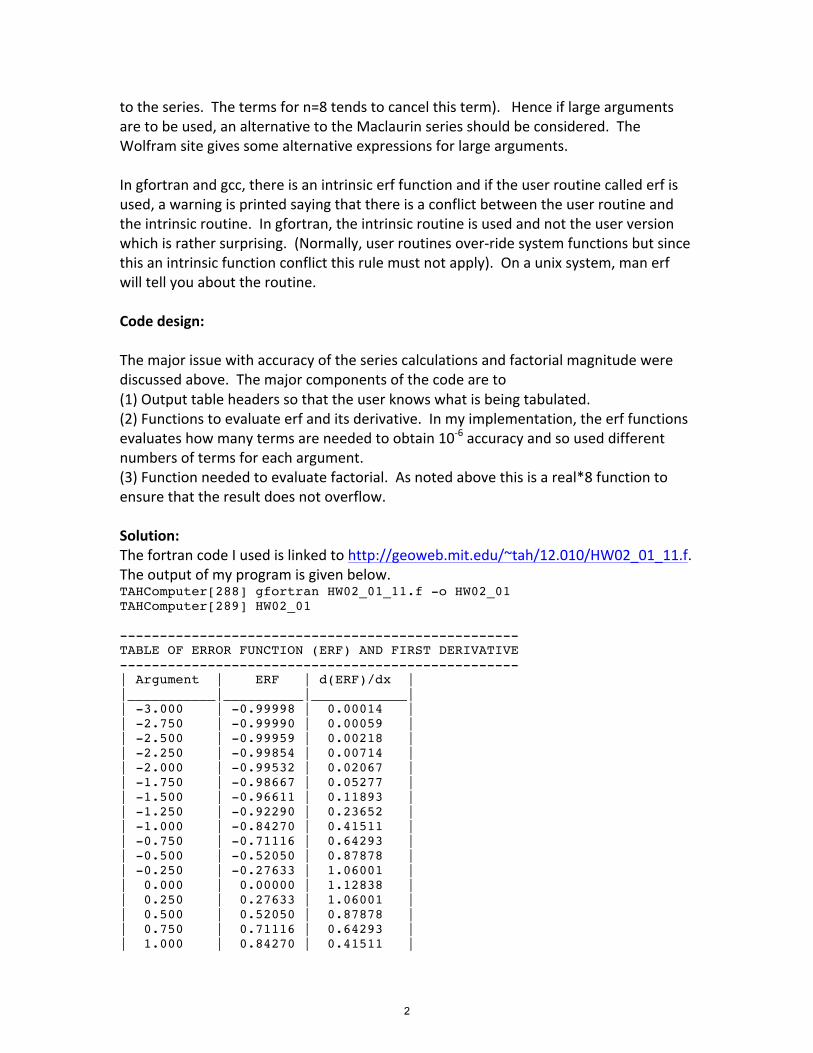
to  the  series.    The  terms  for  n=8  tends  to  cancel  this  term).      Hence  if  large  arguments  are  to  be  used,  an  alternative  to  the  Maclaurin  series  should  be  considered.    The  Wolfram  site  gives  some  alternative  expressions  for  large  arguments.    In  gfortran  and  gcc,  there  is  an  intrinsic  erf  function  and  if  the  user  routine  called  erf  is  used,  a  warning  is  printed  saying  that  there  is  a  conflict  between  the  user  routine  and  the  intrinsic  routine.    In  gfortran,  the  intrinsic  routine  is  used  and  not  the  user  version  which  is  rather  surprising.    (Normally,  user  routines  over-­‐ride  system  functions  but  since  this  an  intrinsic  function  conflict  this  rule  must  not  apply).    On  a  unix  system,  man  erf  will  tell  you  about  the  routine.      Code  design:    The  major  issue  with  accuracy  of  the  series  calculations  and  factorial  magnitude  were  discussed  above.    The  major  components  of  the  code  are  to    (1)  Output  table  headers  so  that  the  user  knows  what  is  being  tabulated.  (2)  Functions  to  evaluate  erf  and  its  derivative.    In  my  implementation,  the  erf  functions  evaluates  how  many  terms  are  needed  to  obtain  10-­‐6  accuracy  and  so  used  different  numbers  of  terms  for  each  argument.  (3)  Function  needed  to  evaluate  factorial.    As  noted  above  this  is  a  real*8  function  to  ensure  that  the  result  does  not  overflow.    Solution:  The  fortran  code  I  used  is  linked  to  http://geoweb.mit.edu/~tah/12.010/HW02_01_11.f.  The  output  of  my  program  is  given  below.  TAHComputer[288] gfortran HW02_01_11.f -o HW02_01 TAHComputer[289] HW02_01 -------------------------------------------------- TABLE OF ERROR FUNCTION (ERF) AND FIRST DERIVATIVE -------------------------------------------------- | Argument | ERF | d(ERF)/dx | |___________|__________|____________| | -3.000 | -0.99998 | 0.00014 | | -2.750 | -0.99990 | 0.00059 | | -2.500 | -0.99959 | 0.00218 | | -2.250 | -0.99854 | 0.00714 | | -2.000 | -0.99532 | 0.02067 | | -1.750 | -0.98667 | 0.05277 | | -1.500 | -0.96611 | 0.11893 | | -1.250 | -0.92290 | 0.23652 | | -1.000 | -0.84270 | 0.41511 | | -0.750 | -0.71116 | 0.64293 | | -0.500 | -0.52050 | 0.87878 | | -0.250 | -0.27633 | 1.06001 | | 0.000 | 0.00000 | 1.12838 | | 0.250 | 0.27633 | 1.06001 | | 0.500 | 0.52050 | 0.87878 | | 0.750 | 0.71116 | 0.64293 | | 1.000 | 0.84270 | 0.41511 |

2

| 1.250 | 0.92290 | 0.23652 | | 1.500 | 0.96611 | 0.11893 | | 1.750 | 0.98667 | 0.05277 | | 2.000 | 0.99532 | 0.02067 | | 2.250 | 0.99854 | 0.00714 | | 2.500 | 0.99959 | 0.00218 | | 2.750 | 0.99990 | 0.00059 | | 3.000 | 0.99998 | 0.00014 | |___________|__________|____________| (b)  How  would  you  change  this  program  if  10  significant  digits  were  required?  Several  changes  would  be  needed  to  output  to  10-­‐signifciant  digits.  

(1) The  format  would  need  to  change  for  the  extra  digits.    In  particular  F8.5  would  need  to  be  changed  to  F14.10  

(2) The  headings  format  would  need  to  be  changed  to  re-­‐align  the  columns  (3) In  the  Erff  function  itself,  the  eps  variable  would  be  changed  to  1.0d-­‐11  to  

ensure  the  10-­‐digits  of  precision  for  the  output.  (4) All  variables  would  need  to  be  real*8.  

Question (2): (25-points). Write  a  program  that  reads  your  name  in  the  form  <first  name>  <middle  name>  <last  name>  and  outputs  the  last  name  first  and  adds  a  comma  after  the  name,  the  first  name,  and  initial  of  your  middle  name  with  a  period  after  the  middle  initial.    If  the  names  start  with  lower  case  letters,  then  these  should  be  capitalized.    The  program  should  not  be  specific  to  the  lengths  of  your  name  (ie.,  the  program  should  work  with  anyone’s  name.  As  an  example.  An  input  of  thomas  abram  herring    would  generate:  Herring,  Thomas  A.    Hints:  Look  at  the  ASCII  table  and  check  the  relationship  between  upper  and  lower  case  letters  Intrinsic  function  CHAR  and  ICHAR  convert  between  character  strings  and  ascii  codes  and  visa  versa.  Reading  with  a  *  format  will  allow  three  strings  to  be  read  on  the  same  line  i.e.,                read(*,*)  string1,  string2,  string3  will  allow  all  names  to  be  on  the  one  line.  Writing  with  a  format  of  a  single  a  (instead  of  a10  for  example)  will  output  only  the  number  of  characters  in  the  string  to  be  output.    To  avoid  extra  spaces,  only  print  the  number  of  characters  needed  using  the  1:N  feature  where  N  is  the  number  of  characters  needed.   Again  a  nominally  easy  program  but  we  will  clearly  need  a  few  utility  subroutines  to  perform  various  tasks.    From  the  question,  the  main  ones  will  be:  

(1) A  subroutine  that  will  convert  a  string  to  upper  case.    Examination  of  the  ASCII  codes  shows  that  the  only  difference  between  upper  and  lower  case  is  that  the  

3

upper  case  symbol  for  a  letter  is  32  less  than  the  lower  case  value.    (man  ascii  on  most  systems  will  print  the  ASCII  table).    Therefore  by  use  of  ICHAR  to  get  the  ASCII  numeric  value  and  CHAR  to  convert  the  ASCII  numeric  value  back  to  a  character,  we  can  convert  from  lower  to  upper  case.    But  we  do  need  to  be  careful:  Only  the  characters  from  a-­‐z  should  be  converted.  

(2) Since  we  need  to  do  other  manipulations  of  strings,  we  will  probably  need  something  that  finds  the  length  of  the  used  portion  of  a  string,  i.e.,  even  though  a  string  may  be  declared  to  a  certain  length  only  some  of  the  string  is  filled  with  non-­‐blank  characters  (in  class  we  discussed  that  fortran  pads  strings  with  blanks  if  a  shorter  length  string  is  assigned  to  a  longer  string  

(3) Since  the  question  calls  for  re-­‐arranging  the  names,  a  routine  that  extracts  “words”  from  a  string  will  be  useful.    An  alternative  would  be  to  read  the  parts  of  the  name  into  different  strings  in  which  case,  this  routine  would  not  be  needed.    This  second  approach  is  used  in  the  homework  solution.  

 For  items  2  and  3  above,  the  routines  will  work  by  finding  the  positions  in  strings  of  blank  and  non-­‐blank  characters  and  using  the  fortran  string(n:m)  feature  to  extract  those  parts  of  the  string.  Code  design  

• Ask  the  user  for  the  string  to  be  converted  and  read  the  user  input.  • Check  for  IOSTAT  errors  reading  the  string    • Check  that  the  string  given  is  not  of  zero-­‐length  (lenline  function).  • Convert  to  upper  case  (tocaps  subroutine-­‐-­‐-­‐  this  could  be  implemented  as  a  

function  since  there  is  only  one  return)  • Extract  each  part  from  it,  namely  first  name,  middle  initial  and  last  name.  

(GetName  routine)  • Check  the  lengths  of  the  parts  of  the  names  to  see  if  zero  length.  • If  the  last  name  is  zero  length,  then  this  implies  that  only  two  parts  of  the  name  

were  entered  so  take  the  second  part  of  name  to  be  last  name  and  make  the  middle  initial  a  question  mark  since  it  does  not  seem  to  have  been  entered.  

• If  the  last  name  still  seems  to  be  zero  length,  then  assume  only  one  name  was  entered  and  so  take  this  to  the  last  name  and  use  question  marks  for  the  first  name  and  middle  initials.  

• Convert  to  upper  case  the  first  letter  of  each  part  of  the  names  (in  case  no  upper  case  given  by  user).      

• Compute  the  lengths  of  each  name  part  and  compute  the  size  of  banner  needed  • Output  banner  and  names  using  the  first  character  only  of  the  middle  name.    

 Routine  tocaps(  in_string,  out_string)  Get  the  minimum  length  of  string  passed  (so  that  we  don’t  exceed  bounds)  Loop  over  each  character  in  string  

If  the  input  character  is  between  ‘a’  and  ‘z’  Subtract  32  from  ASCII  code  and  convert  back  to  character  

4

Endif  End  loop  Function  lenline(inline)  Returns  the  length  of  the  used  portion  (non-­‐blank  character)  of  a  string  Get  the  full  length  of  the  string  Start  at  the  end  of  the  string  working  backwards  to  find  a  non-­‐blank  character.    Make  

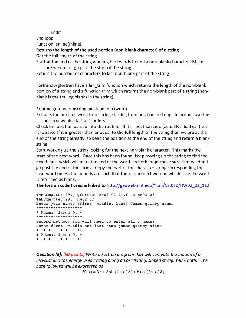
sure  we  do  not  go  past  the  start  of  the  string  Return  the  number  of  characters  to  last  non-­‐blank  part  of  the  string    Fortran90/gfortran  have  a  len_trim  function  which  returns  the  length  of  the  non-­‐blank  portion  of  a  string  and  a  function  trim  which  returns  the  non-­‐blank  part  of  a  string  (non-­‐blank  is  the  trailing  blanks  in  the  string)    Routine  getname(instring,  position,  nextword)  Extracts  the  next  full  word  from  string  starting  from  position  in  string.    In  normal  use  the  

position  would  start  at  1  or  less.  Check  the  position  passed  into  the  routine.    If  it  is  less  than  zero  (actually  a  bad  call)  set  it  to  zero.    If  it  is  greater  than  or  equal  to  the  full  length  of  the  string  then  we  are  at  the  end  of  the  string  already,  so  keep  the  position  at  the  end  of  the  string  and  return  a  blank  string.  Start  working  up  the  string  looking  for  the  next  non-­‐blank  character.    This  marks  the  start  of  the  next  word.    Once  this  has  been  found,  keep  moving  up  the  string  to  find  the  next  blank,  which  will  mark  the  end  of  the  word.    In  both  loops  make  sure  that  we  don’t  go  past  the  end  of  the  string.    Copy  the  part  of  the  character  string  corresponding  the  next  word  unless  the  bounds  are  such  that  there  is  no  next  word  in  which  case  the  word  is  returned  as  blank.  The  fortran  code  I  used  is  linked  to  http://geoweb.mit.edu/~tah/12.010/HW02_02_11.f   TAHComputer[290] gfortran HW02_02_11.f -o HW02_02 TAHComputer[291] HW02_02 Enter your names (First, middle, last) James quincy adams ******************* * Adams, James Q. * ******************* Second method: You will need to enter all 3 names Enter first, middle and last name james quincy adams +++++++++++++++++++ + Adams, James Q. + +++++++++++++++++++ Question  (3):  (50-­‐points)  Write  a  Fortran  program  that  will  compute  the  motion  of  a  bicyclist  and  the  energy  used  cycling  along  an  oscillating,  sloped  straight-­‐line  path.      The  path  followed  will  be  expressed  as  

H (x) = Sx + Asin(2! x / ")+Bcos(2! x / ")  

5

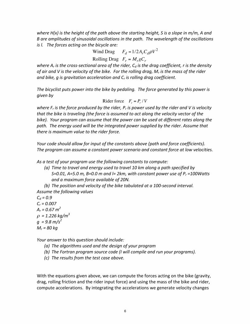
where  H(x)  is  the  height  of  the  path  above  the  starting  height,  S  is  a  slope  in  m/m,  A  and  B  are  amplitudes  of  sinusoidal  oscillations  in  the  path.    The  wavelength  of  the  oscillations  is  l.      The  forces  acting  on  the  bicycle  are:  

 Wind Drag Fd =1/2ArCd V 2"

Rolling Drag Fr = MrgCrwhere  Ar  is  the  cross-­‐sectional  area  of  the  rider,  Cd  is  the  drag  coefficient,  r  is  the  density  of  air  and  V  is  the  velocity  of  the  bike.    For  the  rolling  drag,  Mr  is  the  mass  of  the  rider  and  bike,  g  is  gravitation  acceleration  and  Cr  is  rolling  drag  coefficient.    The  bicyclist  puts  power  into  the  bike  by  pedaling.    The  force  generated  by  this  power  is  given  by  

Rider force Fr = Pr /V  where  Fr  is  the  force  produced  by  the  rider,  Pr  is  power  used  by  the  rider  and  V  is  velocity  that  the  bike  is  traveling  (the  force  is  assumed  to  act  along  the  velocity  vector  of  the  bike).    Your  program  can  assume  that  the  power  can  be  used  at  different  rates  along  the  path.    The  energy  used  will  be  the  integrated  power  supplied  by  the  rider.  Assume  that  there  is  maximum  value  to  the  rider  force.    Your  code  should  allow  for  input  of  the  constants  above  (path  and  force  coefficients).    The  program  can  assume  a  constant  power  scenario  and  constant  force  at  low  velocities.      As  a  test  of  your  program  use  the  following  constants  to  compute:  

(a) Time  to  travel  and  energy  used  to  travel  10  km  along  a  path  specified  by  S=0.01,  A=5.0  m,  B=0.0  m  and  l=  2km,  with  constant  power  use  of  Pr  =100Watts  and  a  maximum  force  available  of  20N.  

(b) The  position  and  velocity  of  the  bike  tabulated  at  a  100-­‐second  interval.  Assume  the  following  values  Cd  =  0.9  Cr  =  0.007  Ar  =  0.67  m

2  ρ    =  1.226  kg/m3  g    =  9.8  m/s2  Mr  =  80  kg    Your  answer  to  this  question  should  include:  

(a) The  algorithms  used  and  the  design  of  your  program  (b) The  Fortran  program  source  code  (I  will  compile  and  run  your  programs).  (c) The  results  from  the  test  case  above.    

   With  the  equations  given  above,  we  can  compute  the  forces  acting  on  the  bike  (gravity,  drag,  rolling  friction  and  the  rider  input  force)  and  using  the  mass  of  the  bike  and  rider,  compute  accelerations.    By  integrating  the  accelerations  we  generate  velocity  changes  

!

6

and  by  integrating  the  velocity  changes  we  get  position  changes.    Since  the  forces  depend  on  velocity,  we  need  to  integrate  in  small  steps.    Precisely  how  small  we  discuss  below.    This  problem  is  basically  an  integration  problem.    It  can  also  be  posed  as  the  solution  to  a  second-­‐order  differential  equation  and  in  later  homework  (and  languages)  we  will  how  to  solve  it  this  way.    There  are  two  basic  ways  of  approaching  this  problem:    (1)  Assume  that  the  bike  remains  attached  to  the  track  (roller  coaster  problem)  and  resolve  the  forces  into  the  direction  of  the  track  at  the  location  of  the  bike  and  assume  that  the  force  perpendicular  to  this  are  balanced  and  can  be  neglected.    In  this  solution,  the  integration  is  along  the  track  and  because  the  track  description  is  given  as  a  function  of  horizontal  distance  and  that  the  total  distance  traveled  is  the  horizontal  distance  (and  not  the  distance  along  the  track),  the  integration  will  need  to  keep  track  of  both  the  distance  along  the  track  and  the  horizontal  distance.    For  a  small  change  in  distance,  the  horizontal  distance  increment  is  dS  cos(theta)  where  theta  is  the  local  slope.  (2)  Compute  the  complete  force  balance  on  the  bike  and  solve  the  equations  in  two  dimensions.    In  this  mode  of  solution,  the  bike  does  not  need  to  stay  on  the  ground.    In  this  solution,  we  need  to  add  gravity  acting  vertically  down,  the  normal  force  from  the  track  surface  which  largely  compensates  gravity  but  because  of  local  slopes  will  also  have  a  component  that  acts  in  the  direction  of  motion  of  the  bike,  and  finally  because  of  the  curvature  of  the  track,  the  centrifugal  and  centripetal  forces  need  to  be  considered.    If  the  force  balance  is  computed  correctly  and  the  bike  is  slow  enough  that  is  does  not  leave  the  track,  the  integration  of  acceleration  and  velocity  to  yield  position  should  trace  out  the  shape  of  the  track.    Both  of  the  above  solutions  are  given  is  the  solution.    In  both  cases,  we  also  add  code  that  allows  the  accuracy  of  the  integrations  to  be  specified.        Since  in  both  solutions  above  we  need  integration  we  should  go  to  the  library  and  read  about  numerical  integration.    Notice  that  there  are  two  parts  to  integration  problems:  (1)  you  need  to  do  the  integration  and  (2)  the  program  has  to  determine  the  accuracy  of  the  integration.    In  particular,  if  the  user  requests  low  accuracy  integration,  then  the  program  should  run  quicker.    In  reading  about  numerical  integration  both  methods  for  integration  and  the  way  of  judging  accuracy  must  be  determined.    You  need  to  know  the  techniques  well  enough  to  implement  in  a  program.  As  discussed  in  the  solution  to  Homework  1,  the  basic  equation  being  integrated  here  the  acceleration  of  the  body.    The  tricky  part  of  the  problem  is  that  the  acceleration  depends  on  the  velocity  of  the  body.    In  the  full  approach,  (2)  above,  we  are  solving  a  pair  of  non-­‐linear  ordinary  differential  equations  in  this  problem.    We  have:  ˙ x ̇ k(x ˙ )2 c(x ˙ ) f (g) 0  " " " =where  x  is  a  vector  of  the  x  and  z  coordinates  of  the  object,  and  the  derivatives  are  with  respect  to  time.  The  k  term  here  is  drag,  c( )  is  the  centripetal  term  and  f(g)  is  the  gravity  and  surface  normal  forces.    In  gene

!ral,  the  integral  above  can  not  be  solved  

analytically  because  the  functions  c  and  f  depend  on  the  track  shape.    

!

7

I  consulted  Numerical  Recipes  (for  the  discussion  of  numerical  integration,  not  the  programs)  and  Abramowitch  and  Stegum.  The  latter  book  gives  the  Runge-­‐Kutta  formula  for  numerically  integrating  an  equation  of  the  form  y’’(x)  =  f(x,y,y’)  where  in  our  case  x  is  time,  y  is  position,  y’  is  velocity  and  y’’  is  acceleration.          

yn+1 = y 'n + h[y 1

n + (k1 + k2 + k3)] O6

+ (h5)

' ' 1yn+1 = yn + [k6 1 + 2k2 + 2k3 + k4 ]

k '1 = hf (xn ,yn,yn )  

k hf (x h /2,y hy ' /2 hk /8,y '2 = n + n + n + 1 n + k1 /2)k hf (x h /2,y hy ' /2 hk /8,y '3 = n + n + n + 1 n + k2 /2)k4 = hf (xn + h,y '

n + hyn + hk3 /2,y'n + k3)

 The  equations  above  give  the  position  (y)  and  velocity  (y’)  at  time  step  n+1  in  the  numerical  integration  based  on  the  values  at  time  step  n.    The  length  of  the  time  step  is  h.    The  O(h^5)  statement  means  that  the  error  in  the  integration  decreases  as  step  size  to  the  5th  power.    The  simple  approach  to  the  numerical  integration  in  Euler’s  method  in  which  the  acceleration  (function  f)  is  computed  for  the  position  and  velocity  at  the  start  of  the  step  and  is  assumed  constant  for  the  distance  traveled  and  velocity  change  during  the  step.    The  above  equation  is  an  approach  (one  of  many  different  ones  available)  in  which  the  constant  acceleration  assumption  is  replaced  with  accelerations  computed  at  different  points  in  the  time  step.    A  very  simple  application  of  this  approach  is  consider  where  gravity  will  be  computed.    Since  the  velocity  of  the  body  is  known  at  the  start  of  the  step,  an  approach  height  at  the  end  of  the  step  can  be  computed  (assuming  constant  velocity)  and  constant  value  of  gravity  used  could  be  computed  at  the  mid-­‐point  of  the  height  at  the  beginning  of  the  step  and  the  approximate  position  at  the  end  of  the  step.    Similarly,  rather  than  computing  drag  using  the  initial  velocity  only,  the  change  in  velocity  can  be  estimated  and  the  drag  computed  using  the  average  velocity  of  the  drag  during  the  step.    The  Runge-­‐Kutta  equations  are  derived  using  these  ideas.    The  Runge-­‐Kutta  integration  method  allows  the  trajectory  to  be  computed  based  in  an  initial  velocity.    Our  problem  is  two-­‐dimensional  and  in  f90  we  could  implement  the  equations  above  uses  two  element  arrays  for  y  and  y’.    In  f77,  we  could  compute  each  component  separately,  or  we  could  use  a  technique  commonly  used  in  2D  problems.    We  can  make  y  and  y’  complex  data  types  where  the  real  component  is  the  x-­‐coordinate  and  the  imaginary  component  is  the  z  coordinate.      One  complication  in  the  integration  here  is  that  we  are  not  integrating  for  a  finite  length  of  time  but  rather  until  the  x-­‐coordinate  reaches  a  set  distance.    This  is  a  bit  tricky  for  the  last  integration  step  where  the  time  interval  until  the  objects  is  not  likely  to  be  the  time  step  being  used  for  the  integration.    The  implementation  in  the  solution  is  to  integrate  until  the  bike  goes  just  past  the  end  of  the  distance.    Smaller  integration  step  sizes  are  made  as  we  approach  the  end.    Based  on  how  far  back  in  time  in  that  last  step,  

!

8

the  last  step  of  the  integration  is  done  with  a  smaller  step  size.    The  last  step  is  repeated  with  smaller  step  sizes  until  the  bike  is  within  the  tolerance  of  the  distance  for  the  accuracy  of  the  calculation.    The  energy  integration  is  done  with  a  a  3-­‐point  Newton-­‐Cotes  Methods  (also  called  Simpson's  rule).    The  one-­‐dimensional  solution  used  the  same  approach  except  that  the  horizontal  coordinate  needs  also  the  integrated.    The  integration  is  built  into  the  Runge-­‐Kutta  integration.      The  basic  flow  of  the  program  is  to:  -­‐Read  the  inputs  fro  the  user.    These  reads  are  ordered  such  that  those  quantities  most  

likely  to  be  changed  by  the  user.  These  values  have  defaults  and  so  the  user  only  needs  to  use  /<cr>  to  adopt  the  defaults.  –  Initialize  the  variables  needed  in  the  program  

-­‐  Trial  integrations  with  decreasing  step  sizes  to  determine  the  step  size  needed  to  hit  the  ground  within  a  specific  accuracy.    In  the  standard  example  we  try  for  10  mm  precision  in  distance  accuracy.  

  The  integration  routine  is  called  Int2d  for  the  two-­‐dimensional  integration  and  Int1d  for  the  one-­‐dimensional  version.      The  routine  called  accel  returns  the  acceleration  at  a  specific  time,  position  and  velocity  (position  is  needed  to  compute  slopes  and  surface  curvature  in  Int2d  (the  latter  is  needed  for  centripetal  force  calculation).    Notice  in  the  2D  version  we  treat  the  X  and  Z  coordinates,  velocities  and  accelerations  as  complex  numbers.    This  allows  the  acceleration  function  to  return  a  complex  result  that  contains  the  X  and  Z  acceleration.    In  the  Runge-­‐Kutta  integration  equations,  I  just  need  one  set  of  expressions  that  do  the  complex  calculations.    (Here  I  just  need  to  be  careful  to  only  multiply  by  real  values  and  to  add  and  subtract  complex  values.)  

-­‐  Once  the  step  size  is  set,  run  with  the  final  step  size  and  output  results.    (This  later  step  is  a  little  inefficient  since  it  repeats  an  earlier  calculation  but  with  output  generated  this  time.    The  output  of  the  trajectory  lines  start  with  T[  *]  and  I  can  use  this  to  extract  using  grep  the  trajectory  of  the  bike.  

Out  put  the  final  velocity  and  the  trajectory  (optional  for  making  plots)    The  program  in  implemented  is  given  in    http://geoweb.mit.edu/~tah/12.010/HW02_03-­‐2D_11.f    for  the  full  two-­‐dimensional  calculation  and  in  http://geoweb.mit.edu/~tah/12.010/HW02_03-­‐1D_11.f    for  the  alternative  formulation  that  uses  the  one-­‐dimensional  integration.    Both  programs  also  uses  an  include  file    http://geoweb.mit.edu/~tah/12.010/FBike.h    that  contains  parameters  for  gravity  values,  air  density  etc  and  a  common  block  that  contains  the  “fixed:”  variables  in  the  program  (object  mass,  drag  coefficient  etc.)  We  also  include  a    

9

http://geoweb.mit.edu/~tah/12.010/HW02_03_11.in  file  that  contains  input  for  the  program.  (Using  /  to  respond  to  the  questions  asked  by  the  program  will  also  generate  the  standard  example  output.)    Example  output  for  test  case:    (HW02_03-2D < HW02_03_11.in >! HW02_03_11.out can also be used. The run bellow uses just default values. These are the values stored in HW02_03_11.in)

 % gfortran HW02_03-2D_11.f -o HW02_03-2D % HW02_03-2D 12.010 Program to solve Bike Motion problem Given track characteristics and rider/bike properties the time, energy and path are computed Program Parameter Input. [Defaults are printed use /<cr> to accept default Length of track (km) and error (mm) [10.000 km 10.0 mm] / Track Slope, Sin and Cos amplitudes (m) and wavelenghth (km) [Defaults 0.001 5.00 m 0.00 m 2.00 km] / Rider/Bike Mass (kg), Area (m**2), Drag and rolling Coefficient ,[ 80.00 kg, 0.670 m^2, 0.90 and 0.0070] / Rider Power (W) and max force (N) [100.00 Watts, 20.00 N] / Output interval, zero for none (default 100.00 s) / ++++++++++++++++++ PROGRAM PARAMETERS ++++++++++++++++++ Length of track 10.000 (km) and error 10.0 (mm) Track Slope 0.001 Sin and Cos amplitudes 5.00 0.00 (m) and wavelenghth 2.00 (km) Rider/Bike Mass 80.00(kg), Area 0.670 (m**2),Drag and rolling Coefficient 0.90 0.0070 Rider Power 100.00 (Watts) and max force 20.00 (N) ++++++++++++++++++++++++++++++++++++++++++++++++++++++++++++ Step size 0.100E+01 s, Times 2255.1473 2255.1669 s Error 195.74 mm Step size 0.500E+00 s, Times 2255.1669 2255.1728 s Error 58.73 mm Step size 0.250E+00 s, Times 2255.1728 2255.1739 s Error 11.37 mm Step size 0.125E+00 s, Times 2255.1739 2255.1741 s Error 2.50 mm O* Time X_pos Z_pos X_vel Z_vel Energy O* (sec) (m) (m) (m/s) (m/s) (Joules) O 0.000 0.0000 0.0000 0.0000 0.0000 0.00 O 100.000 79.9901 1.3233 1.4887 0.0241 1600.02 O 200.000 306.7628 4.4134 3.3670 0.0335 6135.90 O 300.000 826.7974 3.4153 6.7976 -0.0846 15409.05 O 400.000 1513.8127 -3.4814 5.8770 0.0099 25409.05 O 500.000 1951.6809 1.1956 2.9595 0.0489 33914.45 O 600.000 2202.4203 5.1719 2.6542 0.0362 38929.87 O 700.000 2608.5166 7.3207 5.8297 -0.0248 46841.18 O 800.000 3292.8975 -0.6856 6.8882 -0.0586 56841.18 O 900.000 3834.8273 1.3551 3.8825 0.0568 66456.49 O 1000.000 4117.3686 5.9193 2.3535 0.0368 72108.05 O 1100.000 4428.1180 9.3010 4.5333 0.0205 78323.45 O 1200.000 5046.5582 4.3178 7.2497 -0.1054 88273.31 O 1300.000 5681.6964 1.4743 4.9737 0.0472 98273.04 O 1400.000 6035.2522 6.5876 2.4808 0.0412 105344.91 O 1500.000 6294.1703 10.2844 3.3205 0.0347 110523.81 O 1600.000 6803.7014 9.6952 6.7144 -0.0793 119705.43 O 1700.000 7493.5363 2.4943 5.9865 0.0041 129705.43 O 1800.000 7941.4394 7.0264 3.0334 0.0499 138347.80 O 1900.000 8193.4336 11.0479 2.6045 0.0362 143388.33 O 2000.000 8588.7675 13.3952 5.7249 -0.0190 151137.56 O 2100.000 9269.2214 5.5265 6.9632 -0.0656 161137.56 O 2200.000 9821.3690 7.1600 3.9921 0.0571 170825.51

10

O 2255.174 10000.0004 9.9995 2.6501 0.0443 174398.59 Time to travel 10.000 km, 2255.17 seconds, 0.63 hrs Rider Energy 174398.59 Joules, 41654.387 Calories Potential 7839.61 Kinetic 281.00 Joules Final Velocity 2.650 0.044 m/sec

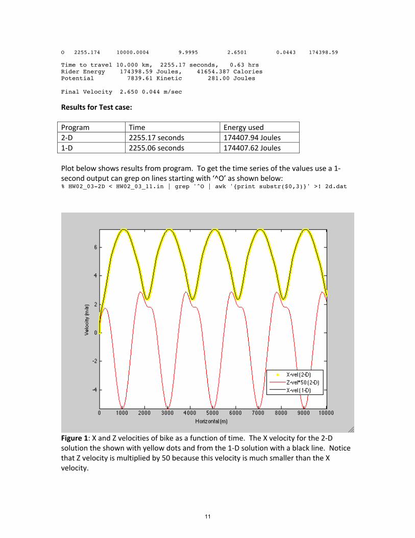
Results  for  Test  case:    Program   Time     Energy  used  2-­‐D   2255.17  seconds   174407.94  Joules  1-­‐D   2255.06  seconds   174407.62  Joules    Plot  below  shows  results  from  program.    To  get  the  time  series  of  the  values  use  a  1-­‐second  output  can  grep  on  lines  starting  with  ‘^O’  as  shown  below:  % HW02_03-2D < HW02_03_11.in | grep '^O | awk '{print substr($0,3)}' >! 2d.dat

Figure  1:  X  and  Z  velocities  of  bike  as  a  function  of  time.    The  X  velocity  for  the  2-­‐D  solution  the  shown  with  yellow  dots  and  from  the  1-­‐D  solution  with  a  black  line.    Notice  that  Z  velocity  is  multiplied  by  50  because  this  velocity  is  much  smaller  than  the  X  velocity.  

11

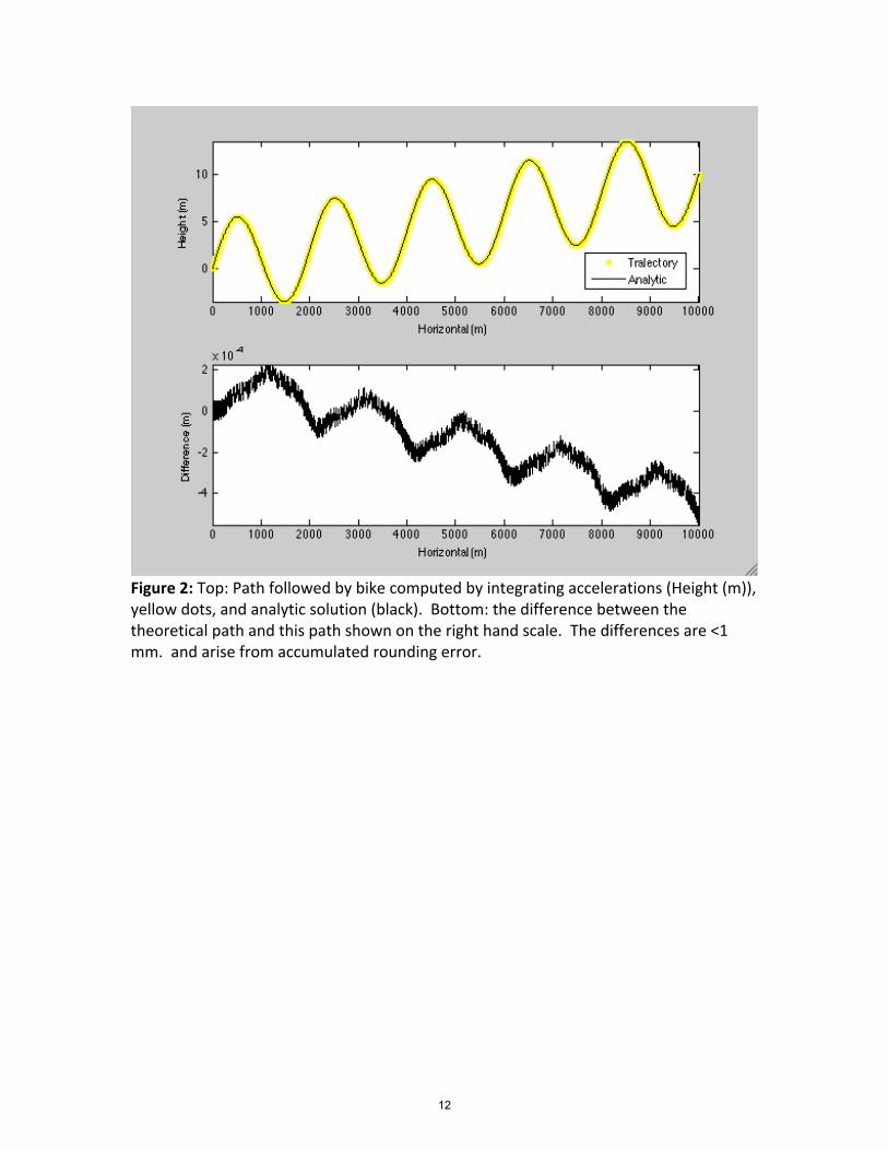
Figure  2:  Top:  Path  followed  by  bike  computed  by  integrating  accelerations  (Height  (m)),  yellow  dots,  and  analytic  solution  (black).    Bottom:  the  difference  between  the  theoretical  path  and  this  path  shown  on  the  right  hand  scale.    The  differences  are  <1  mm.    and  arise  from  accumulated  rounding  error.  

12

MIT OpenCourseWare http://ocw.mit.edu

12.010 Computational Methods of Scientific Programming Fall 2011

For information about citing these materials or our Terms of Use, visit: http://ocw.mit.edu/terms.