11. lecture ws 2014/15 bioinformatics iii1 v11 menger’s theorem borrowing terminology from...

11. Lecture WS 2014/15Bioinformatics III 1

V11 Menger’s theorem

Borrowing terminology from operations research

consider certain primal-dual pairs of optimization

problems that are intimately related.

Usually, one of these problems involves

the maximization of some objective function,

while the other is a minimization problem.

Bioinformatics III 2

Separating setA feasible solution to one of the problems provides a bound for the

optimal value of the other problem (referred to as weak duality),

and the optimal value of one problem is equal to the optimal value

of the other (strong duality).

a u-v separating vertex set is a vertex-cut, and

a u-v separating edge set is an edge-cut.

When the context is clear, the term u-v separating set will refer either to a

u-v separating vertex set or to a u-v separating edge set.

Definition: Let u and v be distinct vertices in a connected graph G.

A vertex subset (or edge subset) S is u-v separating (or separates u and v),

if the vertices u and v lie in different components of the deletion subgraph G – S.

11. Lecture WS 2014/15


Example

For the graph G in the Figure below, the vertex-cut {x,w,z} is a u-v separating set

of vertices of minimum size, and the edge-cut {a,b,c,d,e} is a u-v separating set of

edges of minimum size.

Notice that a minimum-size u-v separating set of edges (vertices) need not be a

minimum-size edge-cut (vertex-cut).

E.g., the set {a,b,c,d,e} is not a minimum-size edge-cut in G, because the set of

edges incident on the 3-valent vertex y is an edge-cut of size 3.



A Primal-Dual Pair of Optimization ProblemsThe connectivity of a graph may be interpreted in two ways.

One interpretation is the number of vertices or edges it takes to disconnect the

graph, and the other is the number of alternative paths joining any two given

vertices of the graph.

Corresponding to these two perspectives are the following two optimization

problems for two non-adjacent vertices u and v of a connected graph G.

Maximization Problem: Determine the maximum number of internally disjoint

u-v paths in graph G.

Minimization Problem: Determine the minimum number of vertices of graph G

needed to separate the vertices u and v.



A Primal-Dual Pair of Optimization ProblemsProposition 5.3.1: (Weak Duality) Let u and v be any two non-adjacent vertices of

a connected graph G. Let Puv be a collection of internally disjoint u-v paths in G,

and let Suv be a u-v separating set of vertices in G.

Then | Puv| ≤ | Suv |.

Proof: Since Suv is a u-v separating set, each u-v path in Puv must include at least

one vertex of Suv . Since the paths in Puv are internally disjoint, no two paths of them

can include the same vertex.

Thus, the number of internally disjoint u-v paths in G is at most | Suv |. □

Corollary 5.3.2. Let u and v be any two non-adjacent vertices of a connected

graph G. Then the maximum number of internally disjoint u-v paths in G is less

than or equal to the minimum size of a u-v separating set of vertices in G.

Menger‘s theorem will show that the two quantities are in fact equal.11. Lecture WS 2014/15


A Primal-Dual Pair of Optimization ProblemsThe following corollary follows directly from Proposition 5.3.1.

Corollary 5.3.3: (Certificate of Optimality) Let u and v be any two non-adjacent

vertices of a connected graph G.

Suppose that Puv is a collection of internally disjoint u-v paths in G,

and that Suv is a u-v separating set of vertices in G, such that | Puv| = | Suv |.

Then Puv is a maximum-size collection of internally disjoint u-v paths, and

Suv is a minimum-size u-v separating set (i.e. S has the smallest size of all u-v

separating sets).



Vertex- and Edge-ConnectivityExample: In the graph G below, the vertex sequences u,x,y,t,v, u,z,v, and

u,r,s,v represent a collection P of three internally disjoint u-v paths in G,

and the set S = {y,s,z} is a u-v separating set of size 3.

Therefore, by Corollary 5.3.3, P is a maximum-size collection of internally disjoint

u-v paths, and S is a minimum-size u-v separating set.

The next theorem proved by K. Menger in 1927 establishes a strong duality

between the two optimization problems introduced earlier.

The proof given here is an example of a traditional style proof in graph theory.

The theorem can also be proven e.g. based on the theory of network flows.



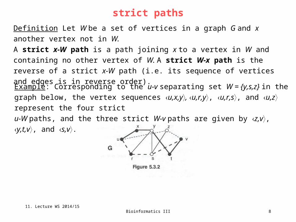
strict paths

Definition Let W be a set of vertices in a graph G and x another vertex not in W.

A strict x-W path is a path joining x to a vertex in W and containing no other vertex

of W. A strict W-x path is the reverse of a strict x-W path (i.e. its sequence of

vertices and edges is in reverse order).

Example: Corresponding to the u-v separating set W = {y,s,z} in the graph below,

the vertex sequences u,x,y, u,r,y, u,r,s, and u,z represent the four strict

u-W paths, and the three strict W-v paths are given by z,v, y,t,v, and s,v.



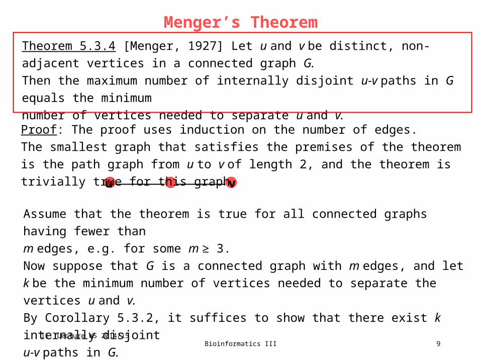
Menger’s TheoremTheorem 5.3.4 [Menger, 1927] Let u and v be distinct, non-adjacent vertices in a

connected graph G.

Then the maximum number of internally disjoint u-v paths in G equals the minimum

number of vertices needed to separate u and v.

u v

Proof: The proof uses induction on the number of edges.

The smallest graph that satisfies the premises of the theorem is the path graph

from u to v of length 2, and the theorem is trivially true for this graph.

Assume that the theorem is true for all connected graphs having fewer than

m edges, e.g. for some m ≥ 3.

Now suppose that G is a connected graph with m edges, and let k be the minimum

number of vertices needed to separate the vertices u and v.

By Corollary 5.3.2, it suffices to show that there exist k internally disjoint

u-v paths in G.

Since this is clearly true if k = 1 (since G is connected), assume k ≥ 2.11. Lecture WS 2014/15


Proof of Menger’s TheoremAssertion 5.3.4a If G contains a u-v path of length 2, then G contains k internally

disjoint u-v paths.

Proof of 5.3.4a: Suppose that P = u,e1,x,e2,v is a path in G of length 2.

Let W be a smallest u-v separating set for the vertex-deletion subgraph G – x.

Since W {x} is a u-v separating set for G, the minimality of k implies that

| W | ≥ k – 1. By the induction hypothesis, there are at least k – 1 internally disjoint u

– v paths in G – x. Path P is internally disjoint from any of these, and, hence,

there are k internally disjoint u-v paths in G. □

If there is a u-v separating set that contains a vertex adjacent to both vertices

u and v, then Assertion 5.3.4a guarantees the existence of k internally disjoint

u-v paths in G.

The argument for distance (u,v) ≥ 3 is now broken into two cases, according to the

kinds of u-v separating sets that exist in G.11. Lecture WS 2014/15


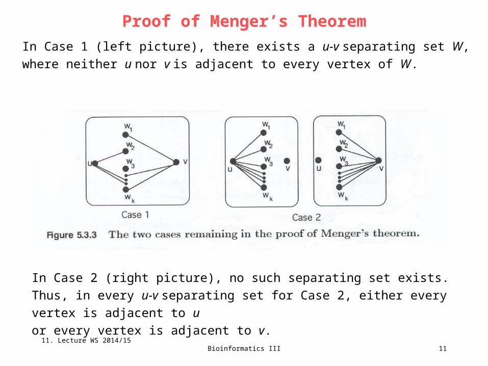
Proof of Menger’s Theorem

In Case 1 (left picture), there exists a u-v separating set W, where neither u nor v is

adjacent to every vertex of W .

In Case 2 (right picture), no such separating set exists.

Thus, in every u-v separating set for Case 2, either every vertex is adjacent to u

or every vertex is adjacent to v.




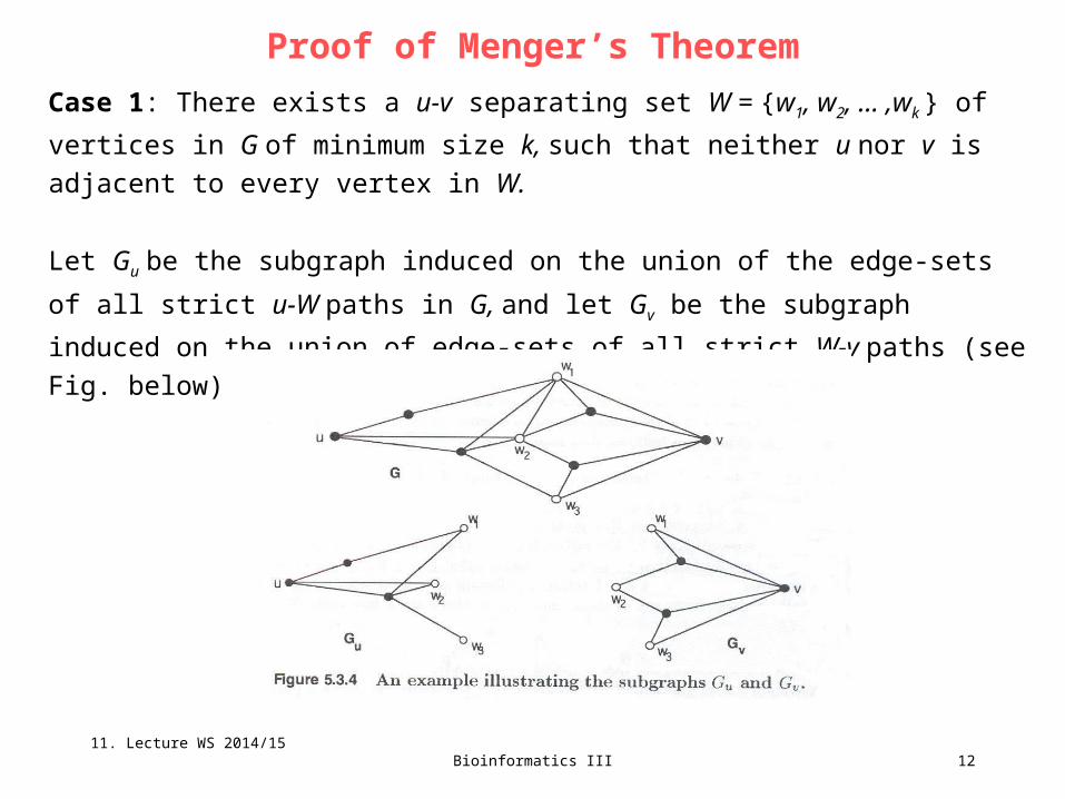
Case 1: There exists a u-v separating set W = {w1, w2, ... ,wk } of vertices in G of

minimum size k, such that neither u nor v is adjacent to every vertex in W.

Let Gu be the subgraph induced on the union of the edge-sets of all strict u-W paths

in G, and let Gv be the subgraph induced on the union of edge-sets of all strict W-v

paths (see Fig. below).




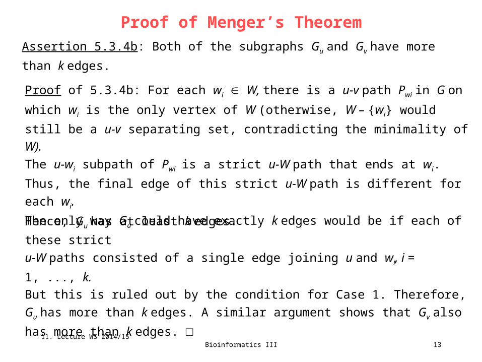
Assertion 5.3.4b: Both of the subgraphs Gu and Gv have more than k edges.

Proof of 5.3.4b: For each wi W, there is a u-v path Pwi in G on which wi is the only

vertex of W (otherwise, W – {wi} would still be a u-v separating set, contradicting the

minimality of W).

The u-wi subpath of Pwi is a strict u-W path that ends at wi.

Thus, the final edge of this strict u-W path is different for each wi.

Hence, Gu has at least k edges.

The only way Gu could have exactly k edges would be if each of these strict

u-W paths consisted of a single edge joining u and wi, i = 1, ..., k.

But this is ruled out by the condition for Case 1. Therefore, Gu has more than k

edges. A similar argument shows that Gv also has more than k edges. □




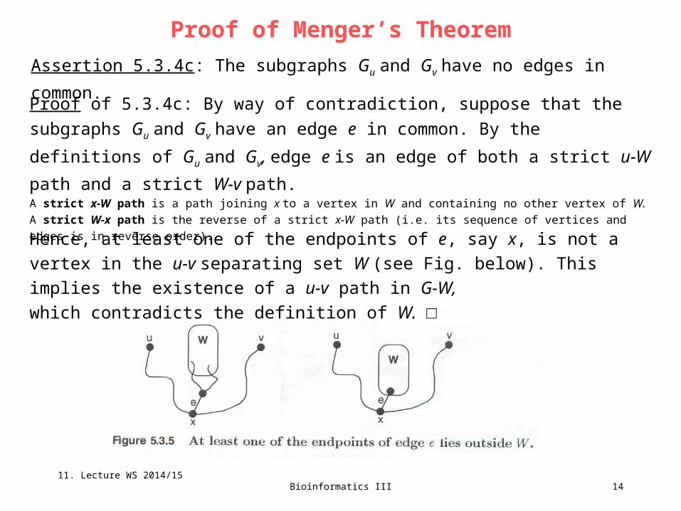
Assertion 5.3.4c: The subgraphs Gu and Gv have no edges in common.

Proof of 5.3.4c: By way of contradiction, suppose that the subgraphs Gu and Gv

have an edge e in common. By the definitions of Gu and Gv, edge e is an edge of

both a strict u-W path and a strict W-v path. A strict x-W path is a path joining x to a vertex in W and containing no other vertex of W.

A strict W-x path is the reverse of a strict x-W path (i.e. its sequence of vertices and edges is in reverse order).

Hence, at least one of the endpoints of e, say x, is not a vertex in the u-v separating

set W (see Fig. below). This implies the existence of a u-v path in G-W,

which contradicts the definition of W. □




We now define two auxiliary graphs Gu* and Gv

*:

Gu* is obtained from G by replacing the subgraph Gv with a new vertex v* and

drawing an edge from each vertex in W to v*, and

Gv* is obtained by replacing Gu with a new vertex u* and drawing an edge from u* to

each vertex in W (see Fig. below).




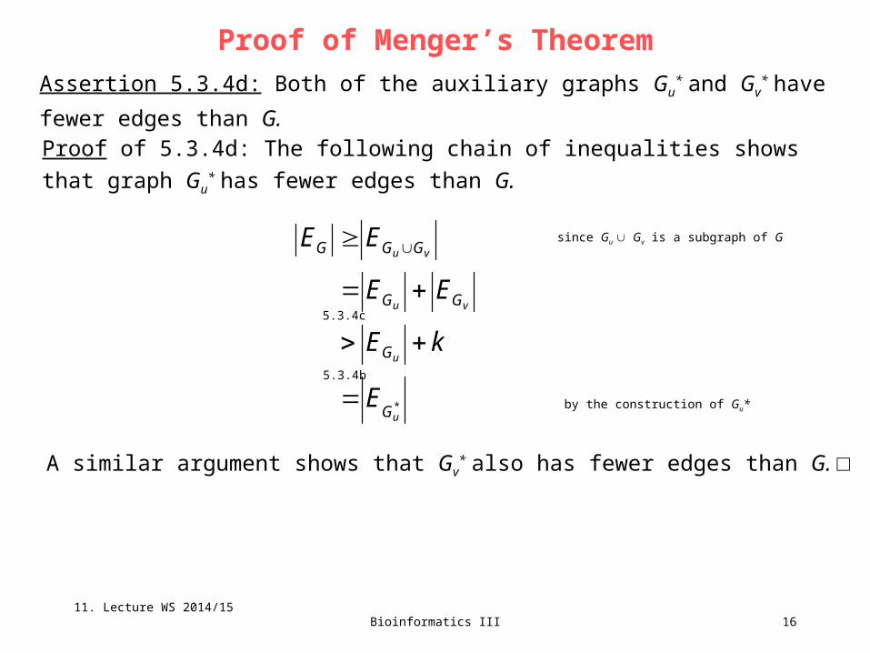
Assertion 5.3.4d: Both of the auxiliary graphs Gu* and Gv

* have fewer edges than G.

*u

u

vu

vu

G

G

GG

GGG

E

kE

EE

EE

A similar argument shows that Gv* also has fewer edges than G. □

5.3.4c

5.3.4b

since Gu Gv is a subgraph of G

by the construction of Gu*

Proof of 5.3.4d: The following chain of inequalities shows that graph Gu* has fewer

edges than G.




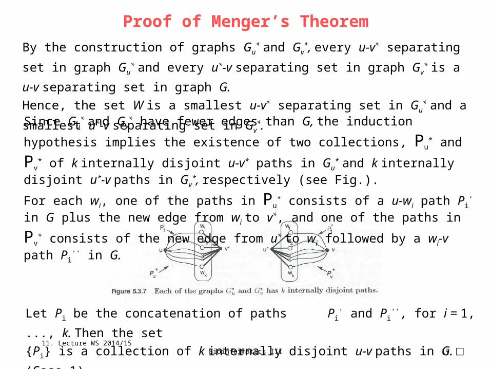
By the construction of graphs Gu* and Gv

*, every u-v* separating set in graph Gu* and

every u*-v separating set in graph Gv* is a u-v separating set in graph G.

Hence, the set W is a smallest u-v* separating set in Gu* and a smallest u*-v

separating set in Gv*.

Since Gu* and Gv

* have fewer edges than G, the induction hypothesis implies the

existence of two collections, Pu* and Pv

* of k internally disjoint u-v* paths in Gu* and

k internally disjoint u*-v paths in Gv*, respectively (see Fig.).

For each wi, one of the paths in Pu* consists of a u-wi path Pi

‘ in G plus the new

edge from wi to v*, and one of the paths in Pv* consists of the new edge from u* to wi

followed by a wi-v path Pi‘‘ in G.

Let Pi be the concatenation of paths Pi‘ and Pi

‘‘, for i = 1, ..., k. Then the set

{Pi} is a collection of k internally disjoint u-v paths in G. □ (Case 1)11. Lecture WS 2014/15



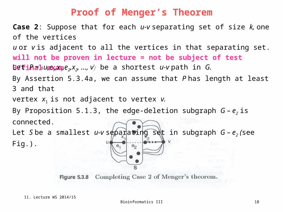
Case 2: Suppose that for each u-v separating set of size k, one of the vertices

u or v is adjacent to all the vertices in that separating set.

will not be proven in lecture = not be subject of test 3/final exam.

Let P = u,e1,x1,e2,x2, ..., v be a shortest u-v path in G.

By Assertion 5.3.4a, we can assume that P has length at least 3 and that

vertex x1 is not adjacent to vertex v.

By Proposition 5.1.3, the edge-deletion subgraph G – e2 is connected.

Let S be a smallest u-v separating set in subgraph G – e2 (see Fig.).




Then S is a u-v separating set in the vertex-deletion subgraph G – x 1.

Thus, S {x1} is a u-v separating set in G, which implies that | S | ≥ k – 1, by the

minimality of k. On the other hand, the minimality of

| S | in G – e2 implies that | S | ≤ k, since every u-v separating set in G is also

a u-v separating set in G – e2.

If | S | = k, then, by the induction hypothesis, there are k internally disjoint u-v paths

in G – e2 and, hence, in G.

If | S | = k – 1, then xi S, i = 1,2 (otherwise S – {xi } would be a u-v separating set

in G – e2, contradicting the minimality of k).

Thus, the sets S {x1} and S {x2} are both of size k and both u-v separating sets

of G. The condition for Case 2 and the fact that vertex x1 is not adjacent to v imply

that every vertex in S is adjacent to vertex u.

Hence, no vertex in S is adjacent to v (lest there be a u-v path of length 2).

But then the condition of Case applied to S { x2 } implies that vertex x2 is adjacent

to vertex u, which contradicts the minimality of path P and completes the proof. □11. Lecture WS 2014/15


V11 – second half

This part follows closely chapter 12.1 in the book on the right

on „Flows and Cuts in Networks and

Chapter 12.2 on “Solving the Maximum-Flow Problem“

Flow in Networks can mean

- flow of oil or water in pipelines, electricity

- phone calls, emails, traffic networks ...

Equivalences between

max-flow min-cut theorem of Ford and Fulkerson

& the connectivity theorems of Menger

led to the development of efficient algorithms for a

number of practical problems to solve scheduling and

assignment problems.



Definition: A single source – single sink network is a connected digraph that

has a distinguished vertex called the source with nonzero outdegree and a

distinguished vertex called the sink with nonzero indegree.

Such a network with source s and sink t is often referred to as a s-t network.

Single Source – Single Sink Capacitated Networks

vetailEevOut N

Correspondingly, In(v) denotes the set of arcs that are directed to vertex v:

veheadEevIn N

Definition: A capacitated network is a connected digraph such that each arc e

is assigned a nonnegative weight cap(e), called the capacity of arc e.

Notation: Let v be a vertex in a digraph N. Then Out(v) denotes the set of all

arcs that are directed from vertex v. That is,



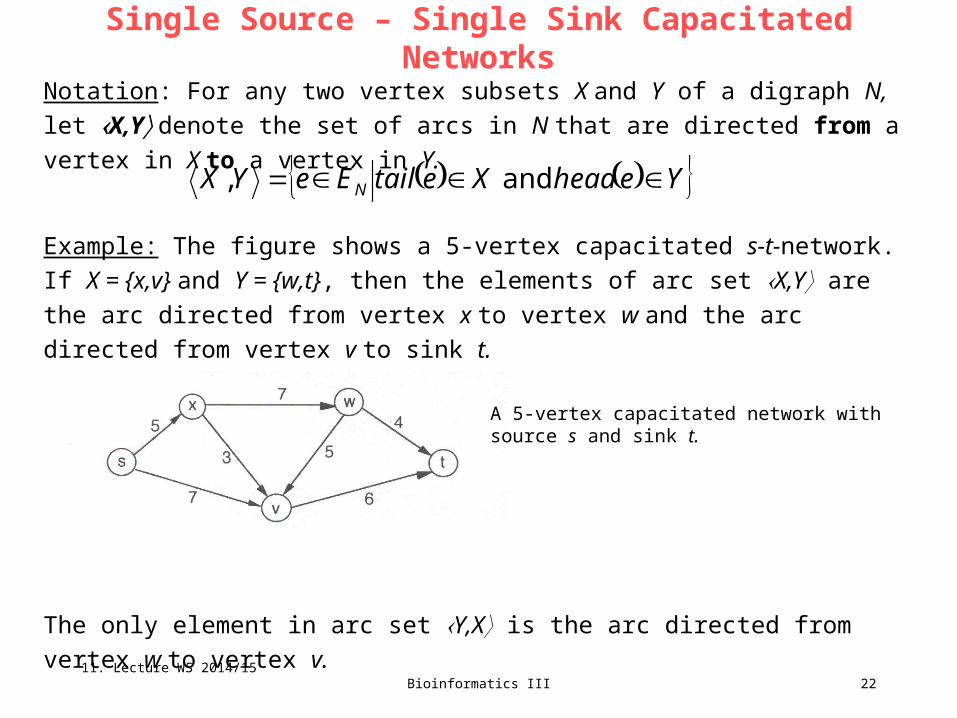
Notation: For any two vertex subsets X and Y of a digraph N, let X,Y denote

the set of arcs in N that are directed from a vertex in X to a vertex in Y.

Single Source – Single Sink Capacitated Networks

YeheadXetailEeYX N and,

Example: The figure shows a 5-vertex capacitated s-t-network.

If X = {x,v} and Y = {w,t}, then the elements of arc set X,Y are the arc directed

from vertex x to vertex w and the arc directed from vertex v to sink t.

The only element in arc set Y,X is the arc directed from vertex w to vertex v.

A 5-vertex capacitated network withsource s and sink t.



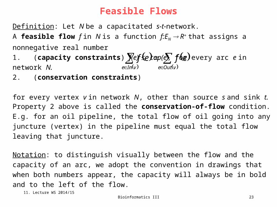
Definition: Let N be a capacitated s-t-network.

A feasible flow f in N is a function f:EN R+ that assigns a nonnegative real number

1. (capacity constraints) f(e) cap(e), for every arc e in network N.

2. (conservation constraints)

for every vertex v in network N, other than source s and sink t.

Feasible Flows

vOutevIne

efef

Property 2 above is called the conservation-of-flow condition.

E.g. for an oil pipeline, the total flow of oil going into any juncture (vertex) in the

pipeline must equal the total flow leaving that juncture.

Notation: to distinguish visually between the flow and the capacity of an arc, we adopt

the convention in drawings that when both numbers appear, the capacity will always

be in bold and to the left of the flow.



Example: The figure shows a feasible flow for the previous network.

Notice that the total amount of flow leaving source s equals 6, which is also the

net flow entering sink t.

Feasible Flows

sInesOute

efeffval

Definition: The maximum flow f* in a capacitated network N is a flow in N

having the maximum value, i.e. val(f) val(f*), for every flow f in N.

Definition: The value of flow f in a capacitated network N, denoted with val(f),

is the net flow leaving the source s, that is



By definition, any nonzero flow must use at least one of the arcs in Out(s).

In other words, if all of the arcs in Out(s) were deleted from network N,

then no flow could get from source s to sink t.

This is a special case of the following definition, which combines the concepts of

partition-cut and s-t separating set.

Cuts in s-t Networks

From V11

Definition: Let G be a graph, and let X1 and X2 form a partition of VG.

The set of all edges of G having one endpoint in X1 and the other endpoint

in X2 is called a partition-cut of G and is denoted X1,X2.

From V12

Definition: Let u and v be distinct vertices in a connected graph G.

A vertex subset (or edge subset) S is u-v separating (or separates u and v),

if the vertices u and v lie in different components of the deletion subgraph G – S.



Definition: Let N be an s-t network, and let Vs and Vt form a partition of VG such

that source s Vs and sink t Vt.

Then the set of all arcs that are directed from a vertex in set Vs to a vertex in set

Vt is called an s-t cut of network N and is denoted Vs,Vt.


Remark: The arc set Out(s) for an s-t network N is the s-t cut {s},VN – {s}, and

In(t) is the s-t cut VN – {t},{t}.



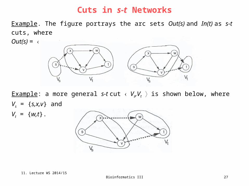
Example. The figure portrays the arc sets Out(s) and In(t) as s-t cuts, where

Out(s) = {s}, {x,v,w,t} and In(t) = {s,x,v,w},{t} .


Example: a more general s-t cut Vs,Vt is shown below, where Vs = {s,x,v} and

Vt = {w,t}.



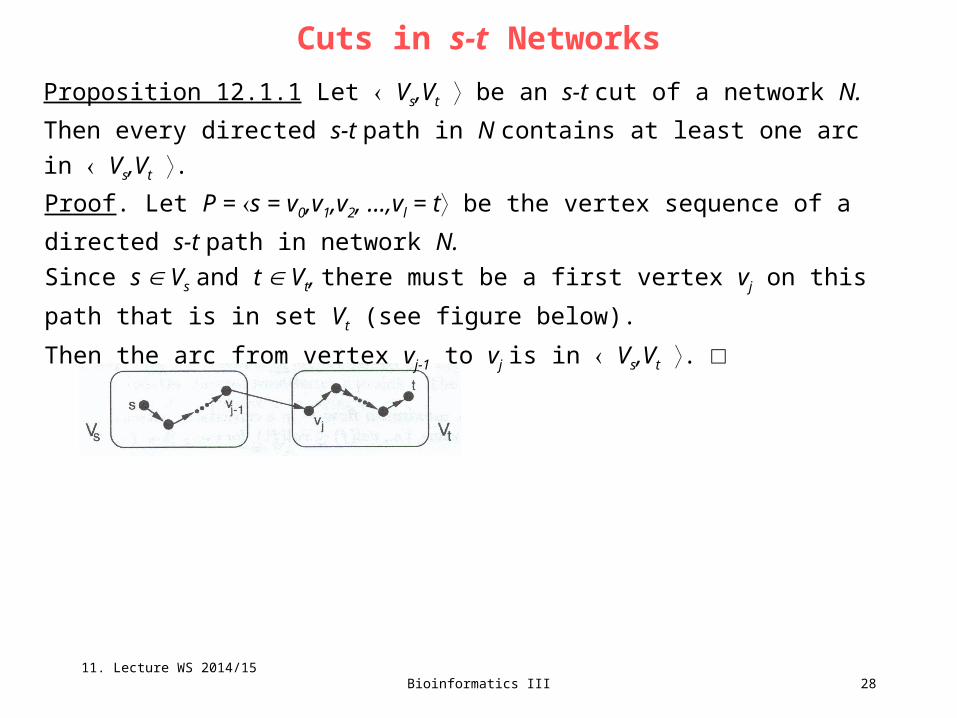
Proposition 12.1.1 Let Vs,Vt be an s-t cut of a network N.

Then every directed s-t path in N contains at least one arc in Vs,Vt .


Proof. Let P = s = v0,v1,v2, …,vl = t be the vertex sequence of a directed s-t path

in network N.

Since s Vs and t Vt, there must be a first vertex vj on this path that is in set Vt

(see figure below).

Then the arc from vertex vj-1 to vj is in Vs,Vt . □



Similar to viewing the set Out(s) of arcs directed from source s as the s-t cut{s}, VN – {s} , the set In(s) may be regarded as the set of „backward“ arcs

relative to this cut, namely, the arc set VN – {s}, {s}, .

From this perspective, the definition of val(f) may be rewritten as

Relationship between Flows and Cuts

ssVesVse NN

efeffval,,



Lemma 12.1.2. Let Vs,Vt be any s-t cut of an s-t network N. Then


stssVv

tsssVv

VVVVvInVVVVvOutss

,, and ,,

Proof: For any vertex v Vs, each arc directed from v is either in Vs,Vs or in

Vs,Vt. The figure illustrates for a vertex v the partition of Out(v) into a 4-element

subset of Vs,Vs and a 3-element subset of Vs,Vt.

Similarly, each arc directed to vertex v is either in Vs,Vs or in Vt,Vs . □

tsVv

ss VVVVvOuts

,,



Proposition 12.1.3. Let f be a flow in an s-t network N, and let Vs,Vt be any s-t

cut of N. Then


stts VVeVVe

efeffval,,

)()( sInesOute

efeffval

Thus . other than every for 0)()(

sVvefef svInevOute

Proof: By definition,

And by the conservation of flow

sss Vv vIneVv vOuteVv vOute vIne

efefefeffval

By Lemma 12.1.2.

stsss

tssss

VVeVVeVv vIne

VVeVVeVv vOute

efefef

efefef

,,

,,

and

(1)

(2)

Now enter the right hand sides of (2) into (1) and obtain the desired equality. □



The flow f and cut {s,x,v},{w,t} shown in the figure illustrate Proposition 12.1.3.

Example

The next corollary confirms something that was apparent from intuition:

the net flow out of the source s equals the net flow into the sink t.

Corollary 12.1.4 Let f be a flow in an s-t network. Then

)()( tOutetIne

efeffval

Proof: Apply proposition 12.1.3 to the s-t cut In(t) = VN – {t}, {t} . □

176,,,,,,,,

vxstwetwvxse

efeffval



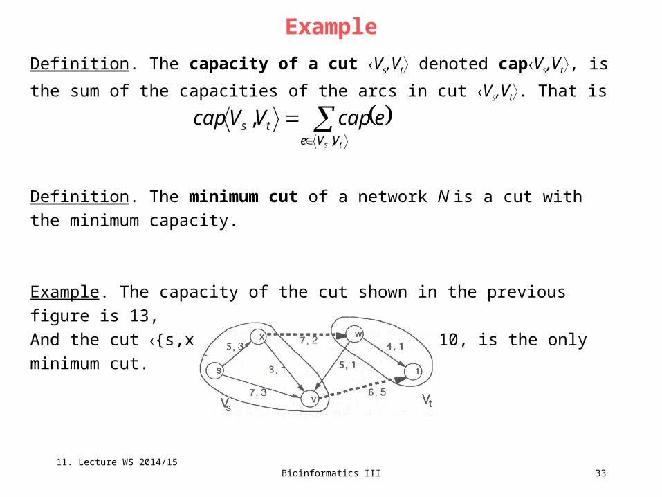
Definition. The capacity of a cut Vs,Vt denoted capVs,Vt, is the sum of the

capacities of the arcs in cut Vs,Vt. That is

Example

ts VVe

ts ecapVVcap,

,

Definition. The minimum cut of a network N is a cut with the minimum capacity.

Example. The capacity of the cut shown in the previous figure is 13,

And the cut {s,x,v,w},{t} with capacity 10, is the only minimum cut.



The problems of finding the maximum flow in a capacitated network N and

finding a minimum cut in N are closely related.

These two optimization problems form a max-min pair.

The following proposition provides an upper bound for the maximum-flow

problem.

Maximum-Flow and Minimum-Cut Problems



Proposition 12.1.5 Let f be any flow in an s-t network, and let Vs,Vt be any s-t cut.

Then


ts VVcapfval ,

Proof:

e)nonnegativ is )(each (since ,

)V, of definition(by ,

s)constraintcapacity (by

12.1.3)n propositio(by

t,

,,

,,

efVVcap

VcapefVVcap

efecap

efeffval

ts

sVVe

ts

VVeVVe

VVeVVe

st

stts

stts

□



Proof: Let f‘ be any feasible flow in network N.

Proposition 12.1.5 and the premise give

On the other hand, let Vs,Vt be any s-t cut. Proposition 12.1.5:

Therefore, K is a minimum cut. □

Corollary 12.1.6 (Weak Duality) Let f* be a maximum flow in an s-t network N,

and let K* be a minimum s-t cut in N. Then


** Kcapfval

Proof: This follows immediately from proposition 12.1.5.

Corollary 12.1.7 (Certificate of Optimality) Let f be a flow in an s-t network N and

K an s-t cut, and suppose that val(f) = cap(K).

Then flow f is a maximum flow in network N, and cut K is a minimum cut.

fvalKcapfval '

ts VVcapfvalKcap ,



Example The flow for the example network shown in the figure has value 10,

which is also the capacity of the s-t cut {s,x,v,w},{t}.By corollary 12.1.7, both the flow and the cut are optimal for their respective

problem.

Example

, if 0

, if

st

ts

VVe

VVeecapef

A maximum flow and minimum cut.

Corollary 12.1.8 Let Vs,Vt be an s-t cut in a network N, and suppose that f is a

flow such that

Then f is a maximum flow in N, and Vs,Vt is a minimum cut.


11. lecture ws 2014/15 bioinformatics iii1 v11 menger’s theorem borrowing terminology from...

Documents

disjoint u

separating set of vertices

minimumsize u

term u

separating vertex set

separating edge set

nonadjacent vertices

minimum number of vertices