1.1 introduction - bharathidasan engineering collegelibrary.bec.ac.in/kbc/notes bec/ece/8 sem/ec...
TRANSCRIPT
BHARATHIDASAN ENGINEERING COLLEGE
LECTURE NOTES ON EC 6801 WIRELESS COMMUNICATION
Prepared by: Prof. C. Narasimhan, Dept. of ECE for V Sem B. Tech. (IT) & VIII Sem ECE
UNIT – I WIRELESS CHANNELS
Large scale path loss – Path loss models: Free Space and Two-Ray models -Link Budget design – Small
scale fading- Parameters of mobile multipath channels – Time dispersion parameters-Coherence
bandwidth – Doppler spread & Coherence time, Fading due to Multipath time delay spread – flat fading –
frequency selective fading – Fading due to Doppler spread – fast fading – slow fading.
1.1 Introduction
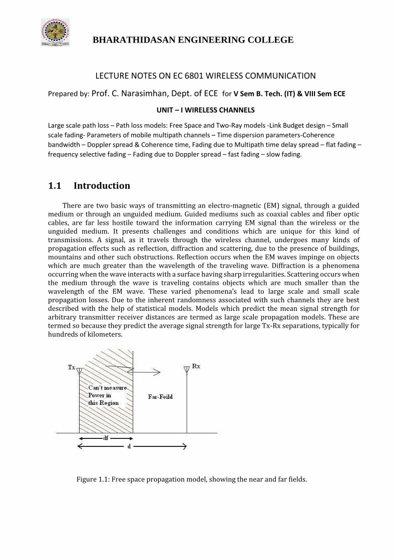
There are two basic ways of transmitting an electro-magnetic (EM) signal, through a guided medium or through an unguided medium. Guided mediums such as coaxial cables and fiber optic cables, are far less hostile toward the information carrying EM signal than the wireless or the unguided medium. It presents challenges and conditions which are unique for this kind of transmissions. A signal, as it travels through the wireless channel, undergoes many kinds of propagation effects such as reflection, diffraction and scattering, due to the presence of buildings, mountains and other such obstructions. Reflection occurs when the EM waves impinge on objects which are much greater than the wavelength of the traveling wave. Diffraction is a phenomena occurring when the wave interacts with a surface having sharp irregularities. Scattering occurs when the medium through the wave is traveling contains objects which are much smaller than the wavelength of the EM wave. These varied phenomena’s lead to large scale and small scale propagation losses. Due to the inherent randomness associated with such channels they are best described with the help of statistical models. Models which predict the mean signal strength for arbitrary transmitter receiver distances are termed as large scale propagation models. These are termed so because they predict the average signal strength for large Tx-Rx separations, typically for hundreds of kilometers.
Figure 1.1: Free space propagation model, showing the near and far fields.

BHARATHIDASAN ENGINEERING COLLEGE
1.2 LARGE SCALE PATH LOSS Free Space Propagation Model
Although EM signals when traveling through wireless channels experience fading effects due to various effects, but in some cases the transmission is with a direct line of sight such as in satellite communication. Free space model predicts that the received power decays as negative square root of the distance. Friis free space equation is given by
(1.1)
where Pt is the transmitted power, Pr(d) is the received power, Gt is the transmitter antenna gain, Gr is the receiver antenna gain, d is the Tx-Rx separation and L is the system loss factor depended upon line attenuation, filter losses and antenna losses and not related to propagation. The gain of the antenna is related to the effective aperture of the antenna which in turn is dependent upon the physical size of the antenna as given below
G = 4πAe/λ2. (1.2)
The path loss, representing the attenuation suffered by the signal as it travels through the wireless channel is given by the difference of the transmitted and received power in dB and is expressed as:
PL(dB) = 10logPt/Pr. (1.3)
The fields of an antenna can broadly be classified in two regions, the far field and the near field. It is in the far field that the propagating waves act as plane waves and the power decays inversely with distance. The far field region is also termed as Fraunhofer region and the Friis equation holds in this region. Hence, the Friis equation is used only beyond the far field distance, df, which is dependent upon the largest dimension of the antenna as df = 2D2/λ. (1.4)
Also we can see that the Friis equation is not defined for d=0. For this reason, we use a close
in distance, do, as a reference point. The power received, Pr(d), is then given by:
Pr(d) = Pr(do)(do/d)2. (1.5)
Ex. 1: Find the far field distance for a circular antenna with maximum dimension of 1 m and operating frequency of 900 MHz. Solution: Since the operating frequency f = 900 Mhz, the wavelength
. Thus, with the largest dimension of the antenna, D=1m, the far field distance is
.

BHARATHIDASAN ENGINEERING COLLEGE
Ex. 2: A unit gain antenna with a maximum dimension of 1 m produces 50 W power at 900 MHz. Find (i) the transmit power in dBm and dB, (ii) the received power at a free space distance of 5 m and 100 m. Solution:
(i) Tx power = 10log(50) = 17 dB = (17+30) dBm = 47 dBm
(ii) d
Thus the received power at 5 m can not be calculated using free space distance formula.
At 100 m ,
= 3.5 × 10⁻³mW PR(dBm) = 10logPr(mW) = −24.5dBm
1.3 Basic Methods of Propagation
Reflection, diffraction and scattering are the three fundamental phenomena that cause signal propagation in a mobile communication system, apart from LoS communication. The most important parameter, predicted by propagation models based on above three phenomena, is the received power. The physics of the above phenomena may also be used to describe small scale fading and multipath propagation. The following subsections give an outline of these phenomena.
1.3.1 Reflection
Reflection occurs when an electromagnetic wave falls on an object, which has very large dimensions as compared to the wavelength of the propagating wave. For example, such objects can be the earth, buildings and walls. When a radio wave falls on another medium having different electrical properties, a part of it is transmitted into it, while some energy is reflected back. Let us see some special cases. If the medium on which the e.m. wave is incident is a dielectric, some energy is reflected back and some energy is transmitted. If the medium is a perfect conductor, all energy is reflected back to the first medium. The amount of energy that is reflected back depends on the polarization of the e.m. wave. Another particular case of interest arises in parallel polarization, when no reflection occurs in the medium of origin. This would occur, when the incident angle would be such that the reflection coefficient is equal to zero. This angle is the Brewster’s angle. By applying laws of electro-magnetics, it is found to be
. (1.6)
Further, considering perfect conductors, the electric field inside the conductor is always zero. Hence all energy is reflected back. Boundary conditions require that
θi = θr (1.7)
BHARATHIDASAN ENGINEERING COLLEGE
and
Ei = Er (1.8) for vertical polarization, and
Ei = −Er (1.9)
for horizontal polarization.
1.3.2 Diffraction
Diffraction is the phenomenon due to which an EM wave can propagate beyond the horizon, around the curved earth’s surface and obstructions like tall buildings. As the user moves deeper into the shadowed region, the received field strength decreases. But the diffraction field still exists an it has enough strength to yield a good signal. This phenomenon can be explained by the Huygen’s principle, according to which, every point on a wavefront acts as point sources for the production of secondary wavelets, and they combine to produce a new wavefront in the direction of propagation. The propagation of secondary wavelets in the shadowed region results in diffraction. The field in the shadowed region is the vector sum of the electric field components of all the secondary wavelets that are received by the receiver.
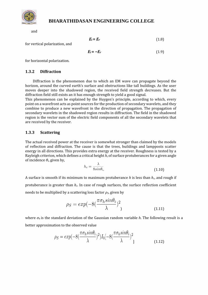
1.3.3 Scattering
The actual received power at the receiver is somewhat stronger than claimed by the models of reflection and diffraction. The cause is that the trees, buildings and lampposts scatter energy in all directions. This provides extra energy at the receiver. Roughness is tested by a Rayleigh criterion, which defines a critical height hc of surface protuberances for a given angle of incidence θi, given by,
. (1.10)
A surface is smooth if its minimum to maximum protuberance h is less than hc, and rough if
protuberance is greater than hc. In case of rough surfaces, the surface reflection coefficient
needs to be multiplied by a scattering loss factor ρS, given by
) (1.11)
where σh is the standard deviation of the Gaussian random variable h. The following result is a
better approximation to the observed value
] (1.12)

BHARATHIDASAN ENGINEERING COLLEGE
which agrees very well for large walls made of limestone. The equivalent reflection coefficient is given by,
Γrough = ρSΓ. (1.13)
1.4 Two Ray Reflection Model
Interaction of EM waves with materials having different electrical properties than the
material through which the wave is traveling leads to transmitting of energy through the
medium and reflection of energy back in the medium of propagation. The amount of energy
reflected to the amount of energy incidented is represented by Fresnel reflection coefficient
Γ, which depends upon the wave polarization, angle of incidence and frequency of the wave.
For example, as the EM waves can not pass through conductors, all the energy is reflected
back with angle of incidence equal to the angle of reflection and reflection coefficient Γ = −1.
In general, for parallel and perpendicular polarizations, Γ is given by:
Γ|| = Er/Ei = η2 sinθt − η1 sinθi/η2 sinθt + η1 sinθi (1.14)
Γ⊥ = Er/Ei = η2 sinθi − η1 sinθt/η2 sinθi + η1 sinθt. (1.15)
Figure 1.2: Two-ray reflection model.
Seldom in communication systems we encounter channels with only LOS paths and hence the Friis formula is not a very accurate description of the communication link. A two-ray model, which consists of two overlapping waves at the receiver, one direct path and one reflected wave from the ground gives a more accurate description as shown in Figure 4.2. A simple addition of a single reflected wave shows that power varies inversely with the forth power of
BHARATHIDASAN ENGINEERING COLLEGE
the distance between the Tx and the Rx. This is deduced via the following treatment. From Figure 4.2, the total transmitted and received electric fields are
ETTOT = Ei + ELOS, (1.16)
ERTOT = Eg + ELOS. (1.17)
Let E0 is the free space electric field (in V/m) at a reference distance d0. Then
) (1.18)
where
(1.19)
and d > d0. The envelop of the electric field at d meters from the transmitter at any time t is therefore
. (1.20)
This means the envelop is constant with respect to time.
Two propagating waves arrive at the receiver, one LOS wave which travels a 0 00 distance of d and another ground reflected wave, that travels d . Mathematically, it can be expressed as:
) (1.21)
where
(1.22)
and
) (1.23)
where
. (1.24)
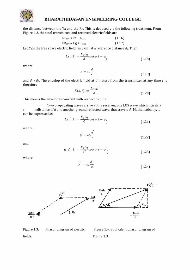
Figure 1.3: Phasor diagram of electric Figure 1.4: Equivalent phasor diagram of
fields. Figure 1.3.
BHARATHIDASAN ENGINEERING COLLEGE
According to the law of reflection in a dielectric, θi = θ0 and Eg = ΓEi which means the total electric field, Et = Ei + Eg = Ei(1 + Γ). (1.25) For small values of θi, reflected wave is equal in magnitude and 180o out of phase with respect to incident wave. Assuming perfect horizontal electric field polarization, i.e., Γ⊥ = −1 =⇒ Et = (1 − 1)Ei = 0, (1.26)
the resultant electric field is the vector sum of ELOS and Eg. This implies that,
ERTOT = |ELOS + Eg|. (1.27)
It can be therefore written that
) (1.28)
In such cases, the path difference is 00 0 q q ∆ = d − d = (ht + hr)2 + d2 − (ht − hr)2 + d2. (1.29) However, when T-R separation distance is very large compared to (ht + hr), then
(1.30)
Ex 3: Prove the above two equations, i.e., equation (1.29) and (1.30).
Once the path difference is known, the phase difference is
(4131) and the time difference,
. (1.32) When d is very large, then ∆ becomes very small and therefore ELOS and Eg are virtually identical with only phase difference,i.e.,
. (1.33)
Say, we want to evaluate the received E-field at any .
Then,
) (1.34)
) (1.35)
(1.36)
(1.37)

BHARATHIDASAN ENGINEERING COLLEGE
Using
phasor diagram concept for vector addition as shown in Figures 1.3 and 1.4, we get
) (1.38)
(1.39)
(1.40)
(1.41)
For . Using equation (1.31) and further equation (1.30),
we can then approximate that
(1.42)
This raises the wonderful concept of ‘cross-over distance’ dc, defined as
. (1.43)
The corresponding approximate received electric field is
. (1.44) Therefore, using equation (4.43) in (4.1), we get the received power as
. (1.45)
The cross-over distance shows an approximation of the distance after which the received
power decays with its fourth order. The basic difference between equation (4.1) and (4.45)
is that when d < dc, equation (4.1) is sufficient to calculate the path loss since the two-ray
model does not give a good result for a short distance due to the oscillation caused by the
constructive and destructive combination of the two rays, but whenever we distance crosses
the ‘cross-over distance’, the power falls off rapidly as well as two-ray model approximation
gives better result than Friis equation.
Observations on Equation (1.45): The important observations from this equation are:
1. This equation gives fair results when the T-R separation distance crosses the cross-over distance.
1. In that case, the power decays as the fourth power of distance

BHARATHIDASAN ENGINEERING COLLEGE
, (1.46)
with K being a constant.
2. Path loss is independent of frequency (wavelength).
3. Received power is also proportional to h2t and h2r, meaning, if height of any of the antennas is increased, received power increases.
1.5 Diffraction
Diffraction is the phenomena that explains the digression of a wave from a straight line path, under the influence of an obstacle, so as to propagate behind the obstacle. It is an inherent feature of a wave be it longitudinal or transverse. For e.g the sound can be heard in a room, where the source of the sound is another room without having any line of sight. The similar phenomena occurs for light also but the diffracted light intensity is not noticeable. This is because the obstacle or slit need to be of the order of the wavelength of the wave to have a significant effect. Thus radiation from a point source radiating in all directions can be received at any
Figure 1.5: Huygen’s secondary wavelets.
point, even behind an obstacle (unless it is not completely enveloped by it), as shown in Figure 1.5. Though the intensity received gets smaller as receiver is moved into the shadowed region. Diffraction is explained by Huygens-Fresnel principle which states that all points on a wavefront can be considered as the point source for secondary wavelets which form the secondary wavefront in the direction of the prorogation. Normally, in absence of an obstacle, the sum of all wave sources is zero at a point not in the direct path of the wave and thus the wave travels in the straight line. But in the case of an obstacle, the effect of wave source behind the obstacle cannot be felt and the sources around the obstacle contribute to the secondary wavelets in the shadowed region, leading to bending of wave. In mobile communication, this has a great advantage since, by diffraction (and scattering, reflection), the receiver is able to receive the signal even when not in line of sight of the transmitter. This we show in the subsection given below.
BHARATHIDASAN ENGINEERING COLLEGE
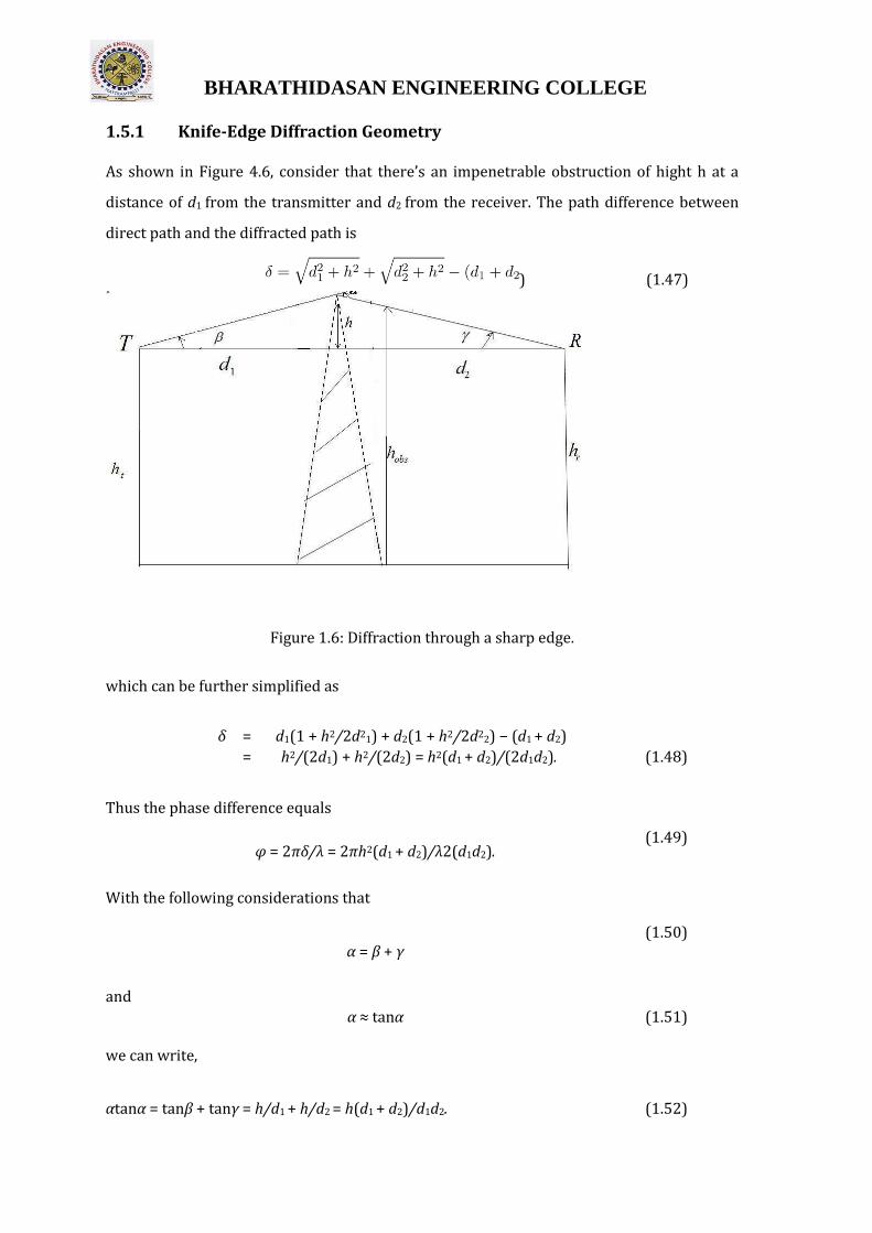
1.5.1 Knife-Edge Diffraction Geometry
As shown in Figure 4.6, consider that there’s an impenetrable obstruction of hight h at a
distance of d1 from the transmitter and d2 from the receiver. The path difference between
direct path and the diffracted path is
) (1.47)
Figure 1.6: Diffraction through a sharp edge.
which can be further simplified as
δ = d1(1 + h2/2d21) + d2(1 + h2/2d22) − (d1 + d2)
= h2/(2d1) + h2/(2d2) = h2(d1 + d2)/(2d1d2). (1.48)
Thus the phase difference equals
φ = 2πδ/λ = 2πh2(d1 + d2)/λ2(d1d2).
With the following considerations that
(1.49)
α = β + γ
and
(1.50)
α ≈ tanα
we can write,
(1.51)
αtanα = tanβ + tanγ = h/d1 + h/d2 = h(d1 + d2)/d1d2. (1.52)

BHARATHIDASAN ENGINEERING COLLEGE
In order to normalize this, we usually use a Fresnel-Kirchoff diffraction parameter v, expressed
as
q q
v = h 2(d1 + d2)/(λd1d2) = α (2d1d2)/(λ(d1 + d2)) (1.53)
Figure 1.7: Fresnel zones.
and therefore the phase difference becomes
φ = πv2/2. (1.54)
From this, we can observe that: (i) phase difference is a function of the height of the
obstruction, and also, (ii) phase difference is a function of the position of the obstruction from
transmitter and receiver.
1.5.2 Fresnel Zones: the Concept of Diffraction Loss
As mentioned before, the more is the object in the shadowed region greater is the diffraction
loss of the signal. The effect of diffraction loss is explained by Fresnel zones as a function of

BHARATHIDASAN ENGINEERING COLLEGE
the path difference. The successive Fresnel zones are limited by the circular periphery
through which the path difference of the secondary waves is nλ/2 greater than total length of
the LOS path, as shown in Figure 4.7. Thus successive Fresnel zones have phase difference of
π which means they alternatively provide constructive and destructive interference to the
received the signal. The radius of the each Fresnel zone is maximum at middle of transmitter
and receiver (i.e. when d1 = d2 ) and decreases as moved to either side. It is seen that the loci
of a Fresnel zone varied over d1 and d2 forms an ellipsoid with the transmitter and receiver
at its focii. Now, if there’s no obstruction, then all Fresnel zones result in only the direct LOS
prorogation and no diffraction effects are observed. But if an obstruction is present,
depending on its geometry, it obstructs contribution from some of the secondary wavelets,
resulting in diffraction and also the loss of energy, which is the vector sum of energy from
unobstructed sources. please note that height of the obstruction can be positive zero and
negative also. The diffraction losses are minimum as long as obstruction doesn’t block volume
of the 1st Fresnel zone. As a rule of thumb, diffraction effects are negligible beyond 55% of
1st Fresnel zone.
Ex 4: Calculate the first Fresnel zone obstruction height maximum for f = 800
MHz.
Solution:
H =
H
Thus H1 = 10 + 6.89 = 16.89m
(b)
Thus
H2 = 10 + 5.6 = 15.48m
. To have good power strength, obstacle should be within the 60% of the first fresnel zone.
Ex 5: Given f=900 MHz, d1 = d2 = 1 km, h = 25m, where symbols have usual
BHARATHIDASAN ENGINEERING COLLEGE
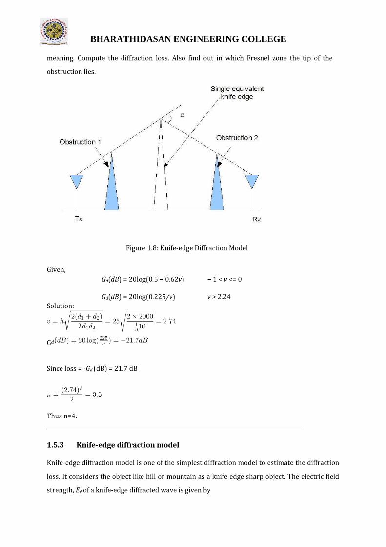
meaning. Compute the diffraction loss. Also find out in which Fresnel zone the tip of the
obstruction lies.
Figure 1.8: Knife-edge Diffraction Model
Given,
Gd(dB) = 20log(0.5 − 0.62v) − 1 < v <= 0
Gd(dB) = 20log(0.225/v) v > 2.24
Solution:
G
Since loss = -Gd (dB) = 21.7 dB
Thus n=4.
1.5.3 Knife-edge diffraction model
Knife-edge diffraction model is one of the simplest diffraction model to estimate the diffraction
loss. It considers the object like hill or mountain as a knife edge sharp object. The electric field
strength, Ed of a knife-edge diffracted wave is given by

BHARATHIDASAN ENGINEERING COLLEGE
(1.55)
The diffraction gain due to presence of knife edge can be given as
Gd(db) = 20log|F(v)| (1.56)
Gd(db) = 0v <= −1 (1.57)
Gd(db) = 20log(0.5 − 0.62) − 1 <= v <= 0 (1.58)
Gd(db) = 20log(0.5exp(−0.95v)) 0 <= v <= 1 (1.59)
Gd(db) = 20log(0.4 − sqrt(0.1184 − (0.38 − 0.1v2))) 1 <= v <= 2.4 (1.60)
Gd(db) = 20log(0.225/v) v > 2.4 (1.61)
When there are more than one obstruction, then the equivalent model can be found by one
knife-edge diffraction model as shown in Figure 4.8.
1.6 Link Budget Analysis
1.6.1 Log-distance Path Loss Model
According to this model the received power at distance d is given by,
) (1.62)
The value of n varies with propagation environments. The value of n is 2 for free space. The
value of n varies from 4 to 6 for obstruction of building, and 3 to 5 for urban scenarios. The
important factor is to select the correct reference distance d0.
For large cell area it is 1 Km, while for micro-cell system it varies from 10m-1m.
Limitations:
Surrounding environmental clutter may be different for two locations having the same
transmitter to receiver separation. Moreover it does not account for the shadowing effects.
1.6.2 Log Normal Shadowing
The equation for the log normal shadowing is given by,
(1.63)
where Xσ is a zero mean Gaussian distributed random variable in dB with standard deviation σ
also in dB. In practice n and σ values are computed from measured

BHARATHIDASAN ENGINEERING COLLEGE
data.
Average received power
The ‘Q’ function is given by,
)) (1.64)
and
Q(z) = 1 − Q(−z) (1.65) So the probability that the received signal level (in dB) will exceed a certain value γ is
. (1.66)
1.7 Multipath Propagation
In wireless telecommunications, multipath is the propagation phenomenon that results in
radio signals reaching the receiving antenna by two or more paths. Causes of multipath
include atmospheric ducting, ionospheric reflection and refraction, and reflection from water
bodies and terrestrial objects such as mountains and buildings. The effects of multipath
include constructive and destructive interference, and phase shifting of the signal. In digital
radio communications (such as GSM) multipath can cause errors and affect the quality of
communications. We discuss all the related issues in this chapter.
1.7.1 Multipath & Small-Scale Fading
Multipath signals are received in a terrestrial environment, i.e., where different forms of
propagation are present and the signals arrive at the receiver from transmitter via a variety
of paths. Therefore there would be multipath interference, causing multipath fading. Adding
the effect of movement of either Tx or Rx or the surrounding clutter to it, the received overall
signal amplitude or phase changes over a small amount of time. Mainly this causes the fading.
1.7.2 Fading
The term fading, or, small-scale fading, means rapid fluctuations of the amplitudes, phases,
or multipath delays of a radio signal over a short period or short travel distance. This might
be so severe that large scale radio propagation loss effects might be ignored.
BHARATHIDASAN ENGINEERING COLLEGE
1.7.3 Multipath Fading Effects
In principle, the following are the main multipath effects:
1. Rapid changes in signal strength over a small travel distance or time interval.
2. Random frequency modulation due to varying Doppler shifts on different multipath signals.
3. Time dispersion or echoes caused by multipath propagation delays.
1.7.4 Factors Influencing Fading
The following physical factors influence small-scale fading in the radio propagation channel:
(1) Multipath propagation – Multipath is the propagation phenomenon that results in radio
signals reaching the receiving antenna by two or more paths. The effects of multipath
include constructive and destructive interference, and phase shifting of the signal.
(2) Speed of the mobile – The relative motion between the base station and the mobile
results in random frequency modulation due to different doppler shifts on each of the
multipath components.
(3) Speed of surrounding objects – If objects in the radio channel are in motion, they
induce a time varying Doppler shift on multipath components. If the surrounding objects
move at a greater rate than the mobile, then this effect dominates fading.
(4) Transmission Bandwidth of the signal – If the transmitted radio signal bandwidth is
greater than the “bandwidth” of the multipath channel (quantified by coherence
bandwidth), the received signal will be distorted.
1.8 Types of Small-Scale Fading
The type of fading experienced by the signal through a mobile channel depends on the
relation between the signal parameters (bandwidth, symbol period) and the channel
parameters (rms delay spread and Doppler spread). Hence we have four different types of
fading. There are two types of fading due to the time dispersive nature of the channel.
BHARATHIDASAN ENGINEERING COLLEGE
1.8.1 Fading Effects due to Multipath Time Delay Spread
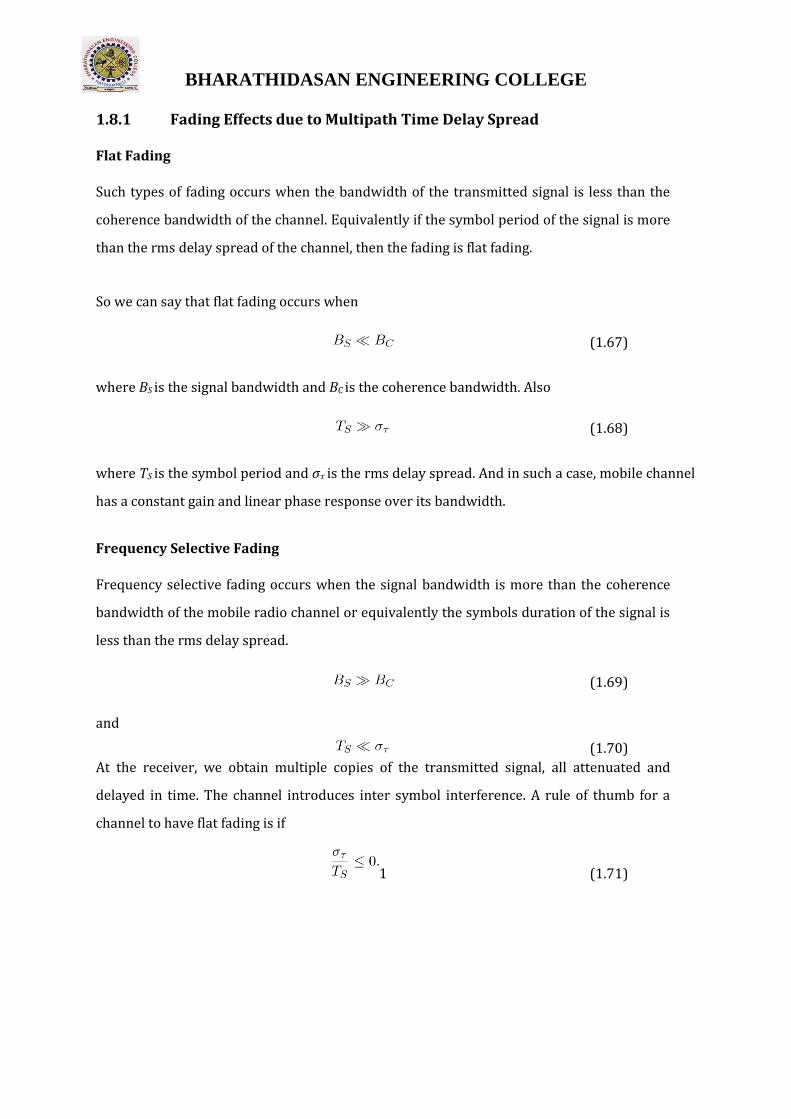
Flat Fading
Such types of fading occurs when the bandwidth of the transmitted signal is less than the
coherence bandwidth of the channel. Equivalently if the symbol period of the signal is more
than the rms delay spread of the channel, then the fading is flat fading.
So we can say that flat fading occurs when
(1.67)
where BS is the signal bandwidth and BC is the coherence bandwidth. Also
(1.68)
where TS is the symbol period and στ is the rms delay spread. And in such a case, mobile channel
has a constant gain and linear phase response over its bandwidth.
Frequency Selective Fading
Frequency selective fading occurs when the signal bandwidth is more than the coherence
bandwidth of the mobile radio channel or equivalently the symbols duration of the signal is
less than the rms delay spread.
(1.69)
and
(1.70)
At the receiver, we obtain multiple copies of the transmitted signal, all attenuated and
delayed in time. The channel introduces inter symbol interference. A rule of thumb for a
channel to have flat fading is if
1 (1.71)

BHARATHIDASAN ENGINEERING COLLEGE
1.8.2 Fading Effects due to Doppler Spread
Fast Fading
In a fast fading channel, the channel impulse response changes rapidly within the symbol
duration of the signal. Due to Doppler spreading, signal undergoes frequency dispersion
leading to distortion. Therefore a signal undergoes fast fading if
(1.72)
where TC is the coherence time and
(1.73)
where BD is the Doppler spread. Transmission involving very low data rates suffer from fast
fading.
Slow Fading
In such a channel, the rate of the change of the channel impulse response is much less than
the transmitted signal. We can consider a slow faded channel a channel in which channel is
almost constant over atleast one symbol duration. Hence
(1.74)
and
(1.75)
We observe that the velocity of the user plays an important role in deciding whether the signal
experiences fast or slow fading.
BHARATHIDASAN ENGINEERING COLLEGE
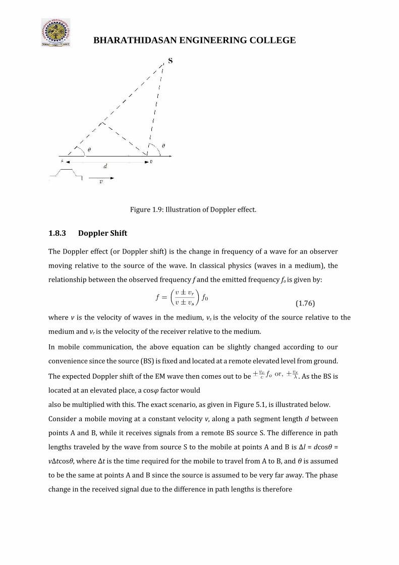
Figure 1.9: Illustration of Doppler effect.
1.8.3 Doppler Shift
The Doppler effect (or Doppler shift) is the change in frequency of a wave for an observer
moving relative to the source of the wave. In classical physics (waves in a medium), the
relationship between the observed frequency f and the emitted frequency fo is given by:
(1.76)
where v is the velocity of waves in the medium, vs is the velocity of the source relative to the
medium and vr is the velocity of the receiver relative to the medium.
In mobile communication, the above equation can be slightly changed according to our
convenience since the source (BS) is fixed and located at a remote elevated level from ground.
The expected Doppler shift of the EM wave then comes out to be . As the BS is
located at an elevated place, a cosφ factor would
also be multiplied with this. The exact scenario, as given in Figure 5.1, is illustrated below.
Consider a mobile moving at a constant velocity v, along a path segment length d between
points A and B, while it receives signals from a remote BS source S. The difference in path
lengths traveled by the wave from source S to the mobile at points A and B is ∆l = dcosθ =
v∆tcosθ, where ∆t is the time required for the mobile to travel from A to B, and θ is assumed
to be the same at points A and B since the source is assumed to be very far away. The phase
change in the received signal due to the difference in path lengths is therefore

BHARATHIDASAN ENGINEERING COLLEGE
(1.77)
and hence the apparent change in frequency, or Doppler shift (fd) is
(1.78)
Example 1
An aircraft is heading towards a control tower with 500 kmph, at an elevation of 20.
Communication between aircraft and control tower occurs at 900 MHz. Find out the expected
Doppler shift. Solution As given here,
v = 500kmph
the horizontal component of the velocity is
v0 = v cosθ = 500 × cos20 = 130m/s
Hence, it can be written that
If the plane banks suddenly and heads for other direction, the Doppler shift change will be 390Hz
to −390Hz.
1.8.4 Impulse Response Model of a Multipath Channel
Mobile radio channel may be modeled as a linear filter with time varying impulse response
in continuous time. To show this, consider time variation due to receiver motion and time
varying impulse response h(d,t) and x(t), the transmitted signal. The received signal y(d,t) at
any position d would be
Z ∞
y(d,t) = x(t) ∗ h(d,t) = x(τ)h(d,t − τ)dτ (1.79) −∞
For a causal system: h(d,t) = 0, for t < 0 and for a stable system
∞
Applying causality condition in the above equation, h(d,t − τ) = 0 for t − τ < 0 ⇒ τ > t, i.e., the
integral limits are changed to

BHARATHIDASAN ENGINEERING COLLEGE
Since the receiver moves along the ground at a constant velocity v, the position of the receiver is
d = vt, i.e.,
Z t
y(vt,t) = x(τ)h(vt,t − τ)dτ. −∞
Since v is a constant, y(vt,t) is just a function of t. Therefore the above equation can be expressed
as
) (1.80)
It is useful to discretize the multipath delay axis τ of the impulse response into equal time
delay segments called excess delay bins, each bin having a time delay width equal to (τi+1 −τi)
= ∆τ and τi = i∆τ for i ∈ 0,1,2,..N −1, where N represents the total number of possible equally-
spaced multipath components, including the first arriving component. The useful frequency
span of the model is 2/∆τ. The model may be used to analyze transmitted RF signals having
bandwidth less than
2/∆τ.
If there are N multipaths, maximum excess delay is given by N∆τ.
y(t) = x(t) ∗ h(t,τi)|i = 0,1,...N − 1
Bandpass channel impulse response model is
(1.81)
x(t) → h(t,τ) = Rehb(t,τ)ejωct → y(t) = Rer(t)ejωct
Baseband equivalent channel impulse response model is given by
(1.82)
) (1.83)
Average power is
(1.84)
The baseband impulse response of a multipath channel can be expressed as
N−1 hb(t,τ) = X ai(t,τ)exp[j(2πfcτi(t) + ϕi(t,τ))]δ(τ − τi(t)) (1.85)
i=0
where ai(t,τ) and τi(t) are the real amplitudes and excess delays, respectively, of the ith
multipath component at time t. The phase term 2πfcτi(t) + ϕi(t,τ) in the above equation

BHARATHIDASAN ENGINEERING COLLEGE
represents the phase shift due to free space propagation of the ith multipath component, plus
any additional phase shifts which are encountered in the channel.
If the channel impulse response is wide sense stationary over a small-scale time or distance
interval, then
N−1
hb(τ) = X ai exp[jθi]δ(τ − τi) (1.86) i=0
For measuring hb(τ), we use a probing pulse to approximate δ(t) i.e.,
p(t) ≈ δ(t − τ) (1.87)
Power delay profile is taken by spatial average of |hb(t,τ)|2 over a local area. The received power
delay profile in a local area is given by
p(τ) ≈ k|hb(t;τ)|2. (1.88)
1.8.5 Relation Between Bandwidth and Received Power
In actual wireless communications, impulse response of a multipath channel is measured
using channel sounding techniques. Let us consider two extreme channel sounding cases.
Consider a pulsed, transmitted RF signal
x(t) = Rep(t)ej2πfct (1.89)
where for 0 ≤ t ≤ Tbb and 0 elsewhere. The low pass channel output
is
.

BHARATHIDASAN ENGINEERING COLLEGE
Figure 5.2: A generic transmitted pulsed RF signal.
The received power at any time t0 is
Interpretation: If the transmitted signal is able to resolve the multipaths, then average
small-scale receiver power is simply sum of average powers received from each multipath
components.
(1.90)
Now instead of a pulse, consider a CW signal, transmitted into the same channel and for simplicity,
let the envelope be c(t) = 2. Then
N−1
r(t) = X ai exp[jθi(t,τ)] (1.91) i=0

BHARATHIDASAN ENGINEERING COLLEGE
and the instantaneous power is
N−1
|r(t)|2 = | X ai exp[jθi(t,τ)]|2 (1.92) i=0
Over local areas, ai varies little but θi varies greatly resulting in large fluctuations.
where rij = Ea[aiaj].
If, rij = cos(θi − θj) = 0, then Ea,θ[PCW ] = Ea,θ[PWB]. This occurs if multipath components are
uncorrelated or if multipath phases are i.i.d over [0,2π].
Bottomline:
1. If the signal bandwidth is greater than multipath channel bandwidth thenfading effects are
negligible
2. If the signal bandwidth is less than the multipath channel bandwidth, largefading occurs
due to phase shift of unresolved paths.
1.8.6 Linear Time Varying Channels (LTV)
The time variant transfer function(TF) of an LTV channel is FT of h(t,τ) w.r.t. τ.
Z ∞
H(f,t) = FT[h(τ,t)] = h(τ,t)e−j2πfτ dτ −∞
(1.93)
Z ∞
h(τ,t) = FT−1[H(f,t)] = H(f,t)ej2πfτ df −∞
The received signal
(1.94)
(1.95)
where R(f,t) = H(f,t)X(f).
For flat fading channel, h(τ,t) = Z(t)δ(τ − τi) where Z(t) = Pαn(t)e−j2πfcτn(t). In this case, the received
signal is

BHARATHIDASAN ENGINEERING COLLEGE
) (1.96)
Figure 1.10: Relationship among different channel functions.
where the channel becomes multiplicative.
Doppler spread functions:
(1.97)
and
(1.98)
Delay Doppler spread:
Z ∞
H(τ,ν) = FT[h(τ,t)] = h(τ,t)e−j2πνtdt (1.99) −∞
1.9 Multipath Channel Parameters
To compare the different multipath channels and to quantify them, we define some
parameters. They all can be determined from the power delay profile. These parameters can
be broadly divided in to two types.

BHARATHIDASAN ENGINEERING COLLEGE
1.9.1 Time Dispersion Parameters
These parameters include the mean excess delay,rms delay spread and excess delay spread. The
mean excess delay is the first moment of the power delay profile and is defined as
(1.100)
where ak is the amplitude, τk is the excess delay and P(τk) is the power of the
individual multipath signals.
The mean square excess delay spread is defined as
(1.101)
Since the rms delay spread is the square root of the second central moment of the power delay
profile, it can be written as
q
στ = τ¯2 − (¯τ)2 (1.102)
As a rule of thumb, for a channel to be flat fading the following condition must be
satisfied
1 (1.103)
where TS is the symbol duration. For this case, no equalizer is required at the
receiver.
Example 2
1. Sketch the power delay profile and compute RMS delay spread for the follow-
ing: 1
P(τ) = P δ(τ − n × 10−6) (in watts) n=0
2. If BPSK modulation is used, what is the maximum bit rate that can be sentthrough the
channel without needing an equalizer?
Solution
1. P(0) = 1 watt, P(1) = 1 watt

BHARATHIDASAN ENGINEERING COLLEGE
τ2 = 0.5µs2 στ = 0.5µs
2. For flat fading channel, we need
For BPSK we need Rb = Rs = 200kbps
Example 3 A simple delay spread bound: Feher’s upper bound
Consider a simple worst-case delay spread scenario as shown in figure below.
Here dmin = d0 and dmax = di + dr
Transmitted power = PT , Minimum received power = PRmin = PThreshold
Put GT = GR = 1 i.e., considering omni-directional unity gain antennas
1.9.2 Frequency Dispersion Parameters
To characterize the channel in the frequency domain, we have the following param-
eters.

BHARATHIDASAN ENGINEERING COLLEGE
(1) Coherence bandwidth: it is a statistical measure of the range of frequencies over which
the channel can be considered to pass all the frequency components with almost equal gain
and linear phase. When this condition is satisfied then we say the channel to be flat.
Practically, coherence bandwidth is the minimum separation over which the two frequency
components are affected differently. If the coherence bandwidth is considered to be the
bandwidth over which the frequency correlation function is above 0.9, then it is
approximated as
. (1.104)
However, if the coherence bandwidth is considered to be the bandwidth over which the
frequency correlation function is above 0.5, then it is defined as
. (1.105)
The coherence bandwidth describes the time dispersive nature of the channel in the local
area. A more convenient parameter to study the time variation of the channel is the coherence
time. This variation may be due to the relative motion between the mobile and the base
station or the motion of the objects in the channel.
(2) Coherence time: this is a statistical measure of the time duration over which the channel
impulse response is almost invariant. When channel behaves like this, it is said to be slow
faded. Essentially it is the minimum time duration over which two received signals are
affected differently. For an example, if the coherence time is considered to be the bandwidth
over which the time correlation is above 0.5, then it can be approximated as
(1.106)
where fm is the maximum doppler spread given be .
Another parameter is the Doppler spread (BD) which is the range of frequencies over which the
received Doppler spectrum is non zero.
1.10 Statistical models for multipath propagation
Many multipath models have been proposed to explain the observed statistical nature of a
practical mobile channel. Both the first order and second order statistics

BHARATHIDASAN ENGINEERING COLLEGE
Figure 1.13: Two ray NLoS multipath, resulting in Rayleigh fading. have been examined in
order to find out the effective way to model and combat the channel effects. The most popular
of these models are Rayleigh model, which describes the NLoS propagation. The Rayleigh
model is used to model the statistical time varying nature of the received envelope of a flat
fading envelope. Below, we discuss about the main first order and second order statistical
models.
1.10.1 NLoS Propagation: Rayleigh Fading Model
Let there be two multipath signals S1 and S2 received at two different time instants due to the
presence of obstacles as shown in Figure 5.6. Now there can either be constructive or
destructive interference between the two signals.
Let En be the electric field and Θn be the relative phase of the various multipath
signals.So we have N
E˜ = X Enejθn (1.107)
n=1
Now if N→ ∞(i.e. are sufficiently large number of multipaths) and all the En are IID distributed,
then by Central Limit Theorem we have,
N
lim E˜ = lim X Enejθn (5.42) N→∞ N→∞ n=1
= Zr + jZi = Rejφ (1.108)
where Zr and Zi are Gaussian Random variables. For the above case
BHARATHIDASAN ENGINEERING COLLEGE
q
R = Zr2 + Zi2 (1.109)
and
(1.110)
For all practical purposes we assume that the relative phase Θn is uniformaly dis-
tributed.
= 0 (1.111)
It can be seen that En and Θn are independent. So,
E[E˜] = E[XEnejθn] = 0 (1.112)
(5.48)
where P0 is the total power obtained. To find the Cumulative Distribution Function(CDF) of R, we
proceed as follows.
Z Z
FR(r) = Pr(R ≤ r) = fZi,Zr(zi,zr)dzidzr (1.113) A
where A is determined by the values taken by the dummy variable r. Let Zi and Zr be zero mean
Gaussian RVs. Hence the CDF can be written as
(1.114)
Let Zr = pcos(Θ) and Zi = psin(Θ) So we have
(1.115)
(1.116)
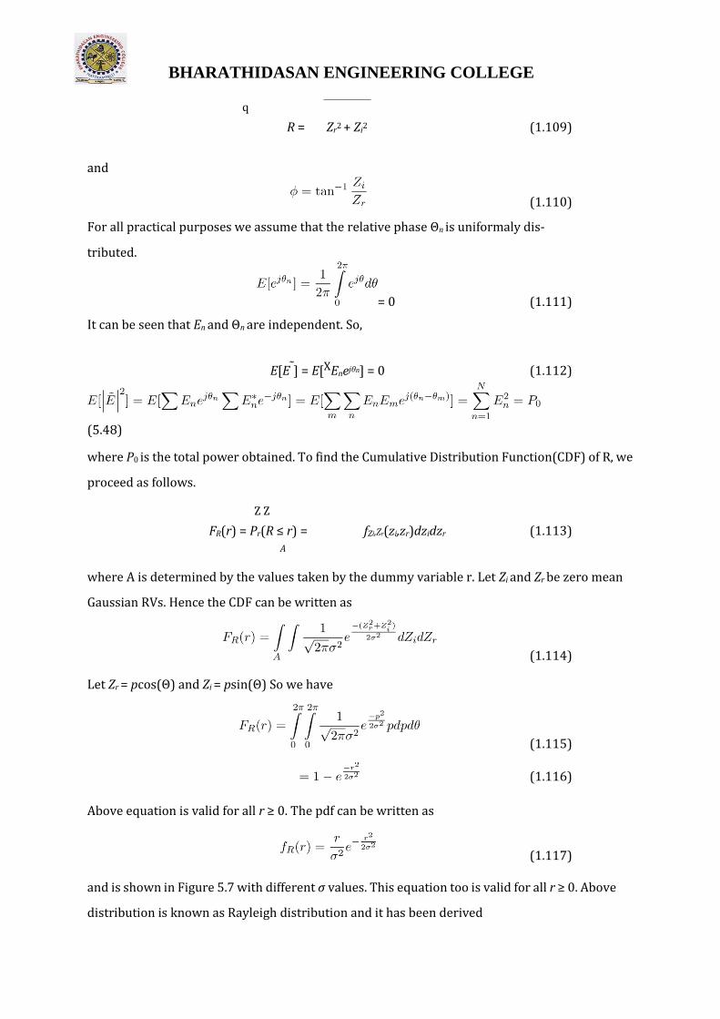
Above equation is valid for all r ≥ 0. The pdf can be written as
(1.117)
and is shown in Figure 5.7 with different σ values. This equation too is valid for all r ≥ 0. Above
distribution is known as Rayleigh distribution and it has been derived

BHARATHIDASAN ENGINEERING COLLEGE
Figure 1.14: Rayleigh probability density function.
for slow fading. However, if 1 Hz, we call it as Quasi-stationary Rayleigh fading. We observe
the following:
(1.118)
(1.119)
(1.120)
(1.121)
1.10.2 LoS Propagation: Rician Fading Model
Rician Fading is the addition to all the normal multipaths a direct LOS path.
Figure 1.15: Ricean probability density function.
) (1.122)

BHARATHIDASAN ENGINEERING COLLEGE
for all A ≥ 0 and r ≥ 0. Here A is the peak amplitude of the dominant signal and
I0(.) is the modified Bessel function of the first kind and zeroth order.
A factor K is defined as
(1.123)
As A → 0 then KdB → ∞.
BHARATHIDASAN ENGINEERING COLLEGE
UNIT II CELLULAR ARCHITECTURE
Multiple Access techniques - FDMA, TDMA, CDMA – Capacity calculations–Cellular concept- Frequency
reuse - channel assignment- hand off- interference & system capacity- trunking & grade of service –
Coverage and capacity improvement.
2.1Multiple Access Techniques for Wireless Communication
In wireless communication systems it is often desirable to allow the subscriber to send
simultaneously information to the base station while receiving information from the base station.
A cellular system divides any given area into cells where a mobile unit in each cell
communicates with a base station. The main aim in the cellular system design is to be able to
increase the capacity of the channel i.e. to handle as many calls as possible in a given bandwidth
with a sufficient level of quality of service. There are several different ways to allow access to the
channel. These includes mainly the following:
1) Frequency division multiple-access (FDMA)
2) Time division multiple-access (TDMA)
3) Code division multiple-access (CDMA)
4) Space Division Multiple access (SDMA)
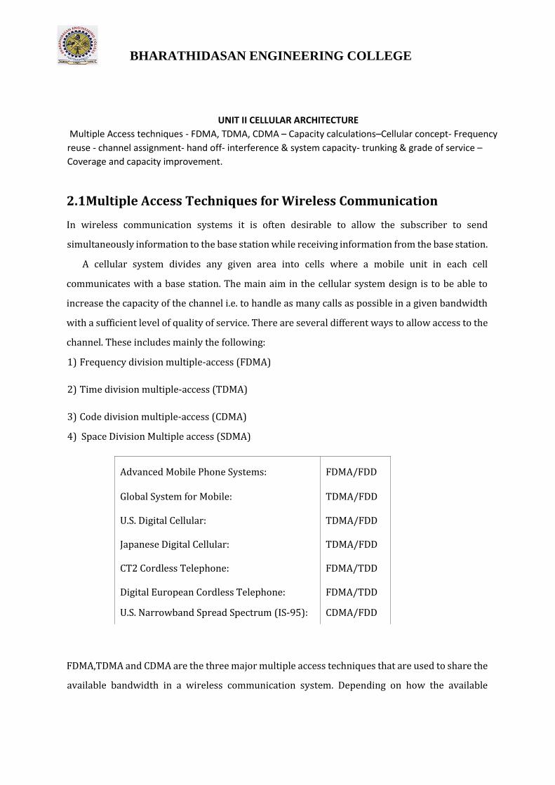
Advanced Mobile Phone Systems: FDMA/FDD
Global System for Mobile: TDMA/FDD
U.S. Digital Cellular: TDMA/FDD
Japanese Digital Cellular: TDMA/FDD
CT2 Cordless Telephone: FDMA/TDD
Digital European Cordless Telephone: FDMA/TDD
U.S. Narrowband Spread Spectrum (IS-95): CDMA/FDD
FDMA,TDMA and CDMA are the three major multiple access techniques that are used to share the
available bandwidth in a wireless communication system. Depending on how the available

BHARATHIDASAN ENGINEERING COLLEGE
bandwidth is allocated to the users these techniques can be classified as narrowband and
wideband systems.
2.1.1 Narrowband Systems
The term narrowband is used to relate the bandwidth of the single channel to the expected
coherence bandwidth of the channel. The available spectrum is divided in to a large number of
narrowband channels. The channels are operated using FDD. In narrow band FDMA, a user is
assigned a particular channel which is not shared by other users in the vicinity and if FDD is used
then the system is called FDMA/FDD. Narrow band TDMA allows users to use the same channel
but allocated a unique time slot to each user on the channel, thus separating a small number of
users in time on a single channel. For narrow band TDMA, there generally are a large number of
channels allocated using either FDD or TDD, each channel is shared using TDMA.
Such systems are called TDMA/FDD and TDMA/TDD access systems.
2.1.2 Wideband Systems
In wideband systems, the transmission bandwidth of a single channel is much larger than the
coherence bandwidth of the channel. Thus, multipath fading doesnt greatly affect the received
signal within a wideband channel, and frequency selective fades occur only in a small fraction of
the signal bandwidth

BHARATHIDASAN ENGINEERING COLLEGE
Figure 2.1: The basic concept of FDMA.
2.2 Frequency Division Multiple Access
This was the initial multiple-access technique for cellular systems in which each individual user
is assigned a pair of frequencies while making or receiving a call as shown in Figure 8.1. One
frequency is used for downlink and one pair for uplink. This is called frequency division duplexing
(FDD). That allocated frequency pair is not used in the same cell or adjacent cells during the call
so as to reduce the co channel interference. Even though the user may not be talking, the spectrum
cannot be reassigned as long as a call is in place. Different users can use the same frequency in
the same cell except that they must transmit at different times.
The features of FDMA are as follows: The FDMA channel carries only one phone circuit at a
time. If an FDMA channel is not in use, then it sits idle and it cannot be used by other users to
increase share capacity. After the assignment of the voice channel the BS and the MS transmit
simultaneously and continuously.
The bandwidths of FDMA systems are generally narrow i.e. FDMA is usually implemented in a
narrow band system The symbol time is large compared to the average delay spread. The

BHARATHIDASAN ENGINEERING COLLEGE
complexity of the FDMA mobile systems is lower than that of TDMA mobile systems. FDMA
requires tight filtering to minimize the
adjacent channel interference.
2.2.1 FDMA/FDD in AMPS
The first U.S. analog cellular system, AMPS (Advanced Mobile Phone System) is based on
FDMA/FDD. A single user occupies a single channel while the call is in progress, and the single
channel is actually two simplex channels which are frequency duplexed with a 45 MHz split. When
a call is completed or when a handoff occurs the channel is vacated so that another mobile
subscriber may use it. Multiple or simultaneous users are accommodated in AMPS by giving each
user a unique signal. Voice signals are sent on the forward channel from the base station to the
mobile unit, and on the reverse channel from the mobile unit to the base station. In AMPS, analog
narrowband frequency modulation (NBFM) is used to modulate the carrier.
2.2.2 FDMA/TDD in CT2
Using FDMA, CT2 system splits the available bandwidth into radio channels in the assigned
frequency domain. In the initial call setup, the handset scans the available channels and locks on
to an unoccupied channel for the duration of the call. Using TDD(Time Division Duplexing ), the
call is split into time blocks that alternate between transmitting and receiving.
2.2.3 FDMA and Near-Far Problem
The near-far problem is one of detecting or filtering out a weaker signal amongst stronger signals.
The near-far problem is particularly difficult in CDMA systems where transmitters share
transmission frequencies and transmission time. In contrast, FDMA and TDMA systems are less
vulnerable. FDMA systems offer different kinds of solutions to near-far challenge. Here, the worst
case to consider is recovery of a weak signal in a frequency slot next to strong signal. Since both
signals are present simultaneously as a composite at the input of a gain stage, the gain is set
according to the level of the stronger signal; the weak signal could be lost in the noise floor. Even
if subsequent stages have a low enough noise floor to provide

BHARATHIDASAN ENGINEERING COLLEGE
2.3 Time Division Multiple Access
In digital systems, continuous transmission is not required because users do not use the allotted
bandwidth all the time. In such cases, TDMA is a complimentary access technique to FDMA. Global
Systems for Mobile communications (GSM) uses the TDMA technique. In TDMA, the entire
bandwidth is available to the user but only for a finite period of time. In most cases the available
bandwidth is divided into fewer channels compared to FDMA and the users are allotted time slots
during which they have the entire channel bandwidth at their disposal, as shown in Figure
2.2.
TDMA requires careful time synchronization since users share the bandwidth in the frequency
domain. The number of channels are less, inter channel interference is almost negligible. TDMA
uses different time slots for transmission and reception. This type of duplexing is referred to as
Time division duplexing(TDD).
The features of TDMA includes the following: TDMA shares a single carrier frequency with
several users where each users makes use of non overlapping time slots. The number of time slots
per frame depends on several factors such as modulation technique, available bandwidth etc.
Data transmission in TDMA is not continuous but occurs in bursts. This results in low battery
consumption since the subscriber transmitter can be turned OFF when not in use. Because of a
discontinuous transmission in TDMA the handoff process is much simpler for a subscriber unit,
since it is able to listen to other base stations during idle time slots. TDMA uses different time
slots for transmission and reception thus duplexers are not required. TDMA has an advantage
that is possible to allocate different numbers of time slots per frame to different users. Thus
bandwidth can be supplied on demand to different users by concatenating or reassigning time
slot based on priority.
2.3.1 TDMA/FDD in GSM
As discussed earlier, GSM is widely used in Europe and other parts of the world. GSM uses a
variation of TDMA along with FDD. GSM digitizes and compresses data, then sends it down a
channel with two other streams of user data, each in its

BHARATHIDASAN ENGINEERING COLLEGE
Figure 2.2: The basic concept of TDMA.
own time slot. It operates at either the 900 MHz or 1800 MHz frequency band. Since many GSM
network operators have roaming agreements with foreign operators, users can often continue to
use their mobile phones when they travel to other countries.
2.3.2 TDMA/TDD in DECT
DECT is a pan European standard for the digitally enhanced cordless telephony using TDMA/TDD.
DECT provides 10 FDM channels in the band 1880-1990 Mhz. Each channel supports 12 users
through TDMA for a total system load of 120 users. DECT supports handover, users can roam over
from cell to cell as long as they remain within the range of the system. DECT antenna can be
equipped with optional spatial diversity to deal with multipath fading.
2.4 Spread Spectrum Multiple Access
Spread spectrum multiple access (SSMA) uses signals which have a transmission bandwidth
whose magnitude is greater than the minimum required RF bandwidth. A pseudo noise (PN)
sequence converts a narrowband signal to a wideband noise like signal before transmission.

BHARATHIDASAN ENGINEERING COLLEGE
SSMA is not very bandwidth efficient when used by a single user. However since many users can
share the same spread spectrum bandwidth without interfering with one another, spread
spectrum systems become bandwidth efficient in a multiple user environment.
There are two main types of spread spectrum multiple access techniques: Frequency hopped
multiple access (FHMA) Direct sequence multiple access (DSMA) or Code division multiple access
(CDMA).
2.4.1 Frequency Hopped Multiple Access (FHMA)
This is a digital multiple access system in which the carrier frequencies of the individual users are
varied in a pseudo random fashion within a wideband channel. The digital data is broken into
uniform sized bursts which is then transmitted on
different carrier frequencies.
2.4.2 Code Division Multiple Access
In CDMA, the same bandwidth is occupied by all the users, however they are all assigned separate
codes, which differentiates them from each other (shown in Figure 8.3). CDMA utilize a spread
spectrum technique in which a spreading signal (which is uncorrelated to the signal and has a
large bandwidth) is used to spread the narrow band message signal.
Direct Sequence Spread Spectrum (DS-SS)
This is the most commonly used technology for CDMA. In DS-SS, the message signal is multiplied
by a Pseudo Random Noise Code. Each user is given his own codeword which is orthogonal to the
codes of other users and in order to detect the user, the receiver must know the codeword used
by the transmitter. There are, however, two problems in such systems which are discussed in the
sequel.

BHARATHIDASAN ENGINEERING COLLEGE
Figure 2.3: The basic concept of CDMA.
CDMA/FDD in IS-95
In this standard, the frequency range is: 869-894 MHz (for Rx) and 824-849 MHz
(for Tx). In such a system, there are a total of 20 channels and 798 users per channel. For each
channel, the bit rate is 1.2288 Mbps. For orthogonality, it usually combines 64 Walsh-Hadamard
codes and a m-sequence.
2.4.3 CDMA and Self-interference Problem
In CDMA, self-interference arises from the presence of delayed replicas of signal due to multipath.
The delays cause the spreading sequences of the different users to lose their orthogonality, as by
design they are orthogonal only at zero phase offset. Hence in despreading a given user’s
waveform, nonzero contributions to that user’s signal arise from the transmissions of the other
users in the network. This is distinct from both TDMA and FDMA, wherein for reasonable time or
frequency guardbands, respectively, orthogonality of the received signals can be preserved.

BHARATHIDASAN ENGINEERING COLLEGE
2.4.4 CDMA and Near-Far Problem
The near-far problem is a serious one in CDMA. This problem arises from the fact that signals
closer to the receiver of interest are received with smaller attenuation than are signals located
further away. Therefore the strong signal from the nearby transmitter will mask the weak signal
from the remote transmitter. In TDMA and FDMA, this is not a problem since mutual interference
can be filtered. In CDMA, however, the near-far effect combined with imperfect orthogonality
between codes (e.g. due to different time sifts), leads to substantial interference. Accurate and
fast power control appears essential to ensure reliable operation of multiuser DS-CDMA systems.
2.4.5 Hybrid Spread Spectrum Techniques
The hybrid combinations of FHMA, CDMA and SSMA result in hybrid spread spectrum techniques
that provide certain advantages. These hybrid techniques are explained below,
Hybrid FDMA/CDMA (FCDMA):
An alternative to the CDMA technique in which the available wideband spectrum is divided
into a smaller number of sub spectra with smaller bandwidths. The smaller sub channels become
narrow band CDMA systems with processing gain lower than the original CDMA system. In this
scheme the required bandwidth need not be contiguous and different user can be allotted
different sub spectrum bandwidths depending on their requirements. The capacity of this hybrid
FCDMA technique is given by the sum of the capacities of a system operating in the sub spectra.
Hybrid Direct Sequence/Frequency Hopped Multiple Access Techniques (DS/FHMA):
A direct sequence modulated signal whose center frequency is made to hop periodically in a
pseudo random fashion is used in this technique. One of the advantages using this technique is
they avoid near-far effect. However, frequency hopped CDMA systems are not adaptable to the
soft handoff process since it is difficult to synchronize the frequency hopped base station receiver
to the multiple hopped signals. Time and Code Division Multiple Access (TCDMA):
In this TCDMA method different cells are allocated different spreading codes.
In each cell, only one user per cell is allotted a particular time slot. Thus at any
time only one user is transmitting in each cell. When a handoff takes place the spreading code of
that user is changed to the code of the new cell. TCDMA also avoids near-far effect as the number
of users transmitting per cell is one.
Time Division Frequency Hopping (TDFH):
This technique has been adopted for the GSM standard, where the hopping sequence is
predefined and the subscriber is allowed to hop only on certain frequencies which are assigned

BHARATHIDASAN ENGINEERING COLLEGE
to a cell. The subscriber can hop to a new frequency at the start of a new TDMA frame, thus
avoiding a severe fade or erasure event on a particular channel. This technique has the advantage
in severe multipath or when severe channel interference occurs.
2.5 Space Division Multiple Access
SDMA utilizes the spatial separation of the users in order to optimize the use of the frequency
spectrum. A primitive form of SDMA is when the same frequency is reused in different cells in a
cellular wireless network. The radiated power of each user is controlled by Space division
multiple access. SDMA serves different users by using spot beam antenna. These areas may be
served by the same frequency or different frequencies. However for limited co-channel
interference it is required that the cells be sufficiently separated. This limits the number of cells
a region can be divided into and hence limits the frequency re-use factor. A more advanced
approach can further increase the capacity of the network. This technique would enable
frequency re-use within the cell. In a practical cellular environment it is improbable to have just
one transmitter fall within the receiver beam width. Therefore it becomes imperative to use other
multiple access techniques in conjunction with SDMA. When different areas are covered by the
antenna beam, frequency can be re-used, in which case TDMA or CDMA is employed, for different
frequencies FDMA can be used.
Cellular concept
Introduction
Communication is one of the integral parts of science that has always been a focus point for
exchanging information among parties at locations physically apart. After its discovery,
telephones have replaced the telegrams and letters. Similarly, the term ‘mobile’ has
completely revolutionized the communication by opening up innovative applications that are
limited to one’s imagination. Today, mobile communication has become the backbone of the
society. All the mobile system technologies have improved the way of living. Its main plus
point is that it has privileged a common mass of society. In this chapter, the evolution as well
as the fundamental techniques of the mobile communication is discussed.

BHARATHIDASAN ENGINEERING COLLEGE
Evolution of Mobile Radio Communications
The first wireline telephone system was introduced in the year 1877. Mobile communication
systems as early as 1934 were based on Amplitude Modulation (AM) schemes and only
certain public organizations maintained such systems. With the demand for newer and better
mobile radio communication systems during the World War II and the development of
Frequency Modulation (FM) technique by Edwin Armstrong, the mobile radio
communication systems began to witness many new changes. Mobile telephone was
introduced in the year 1946. However, during its initial three and a half decades it found very
less market penetration owing to high
Figure The worldwide mobile subscriber chart.
costs and numerous technological drawbacks. But with the development of the cellular
concept in the 1960s at the Bell Laboratories, mobile communications began to be a
promising field of expanse which could serve wider populations. Initially, mobile
communication was restricted to certain official users and the cellular concept was never
even dreamt of being made commercially available. Moreover, even the growth in the cellular
networks was very slow. However, with the development of newer and better technologies
starting from the 1970s and with the mobile users now connected to the Public Switched
Telephone Network (PSTN), there has been an astronomical growth in the cellular radio and
the personal communication systems. Advanced Mobile Phone System (AMPS) was the first

BHARATHIDASAN ENGINEERING COLLEGE
U.S. cellular telephone system and it was deployed in 1983. Wireless services have since then
been experiencing a 50% per year growth rate. The number of cellular telephone users grew
from 25000 in 1984 to around 3 billion in the year 2007 and the demand rate is increasing
day by day. A schematic of the subscribers is shown in Fig. 1.1.
Figure Basic mobile communication structure.
Present Day Mobile Communication
Since the time of wireless telegraphy, radio communication has been used extensively. Our
society has been looking for acquiring mobility in communication since then. Initially the
mobile communication was limited between one pair of users on single channel pair. The
range of mobility was defined by the transmitter power, type of antenna used and the
frequency of operation. With the increase in the number of users, accommodating them
within the limited available frequency spectrum became a major problem. To resolve this
problem, the concept of cellular communication was evolved. The present day cellular
communication uses a basic unit called cell. Each cell consists of small hexagonal area with a
base station located at the center of the cell which communicates with the user. To
accommodate multiple users Time Division multiple Access (TDMA), Code Division Multiple

BHARATHIDASAN ENGINEERING COLLEGE
Access (CDMA), Frequency Division Multiple Access (FDMA) and their hybrids are used.
Numerous mobile radio standards have been deployed at various places such as AMPS, PACS,
Figure The basic radio transmission techniques: (a) simplex, (b) half duplex and (c) full duplex.
GSM, NTT, PHS and IS-95, each utilizing different set of frequencies and allocating different
number of users and channels.
Fundamental Techniques
By definition, mobile radio terminal means any radio terminal that could be moved during its
operation. Depending on the radio channel, there can be three different types of mobile
communication. In general, however, a Mobile Station (MS) or subscriber unit communicates
to a fixed Base Station (BS) which in turn communicates to the desired user at the other end.
The MS consists of transceiver, control circuitry, duplexer and an antenna while the BS
consists of transceiver and channel multiplexer along with antennas mounted on the tower.
The BS are also linked to a power source for the transmission of the radio signals for
communication and are connected to a fixed backbone network. Figure 1.2 shows a basic

BHARATHIDASAN ENGINEERING COLLEGE
mobile communication with low power transmitters/receivers at the BS, the MS and also the
Mobile Switching Center (MSC). The MSC is sometimes also called Mobile Telephone
Switching Office (MTSO). The radio signals emitted by the BS decay as the signals travel away
from it. A minimum amount of signal strength is needed in order to be detected by the mobile
stations or mobile sets which are the hand-held personal units (portables) or those installed
in the vehicles (mobiles). The region over which the signal strength lies above such a
threshold value is known as the coverage area of a BS. The fixed backbone network is a wired
network that links all the base stations and also the landline and other telephone networks
through wires.
Radio Transmission Techniques
Based on the type of channels being utilized, mobile radio transmission systems may be
classified as the following three categories which is also shown in Fig. 1.3:
• Simplex System: Simplex systems utilize simplex channels i.e., the communication is
unidirectional. The first user can communicate with the second user. However, the
second user cannot communicate with the first user. One example of such a system is a
pager.
• Half Duplex System: Half duplex radio systems that use half duplex radio channels
allow for non-simultaneous bidirectional communication. The first user can
communicate with the second user but the second user can communicate to the first
user only after the first user has finished his conversation. At a time, the user can only
transmit or receive information. A walkie-talkie is an example of a half duplex system
which uses ‘push to talk’ and ‘release to listen’ type of switches.
• Full Duplex System: Full duplex systems allow two way simultaneous
communications. Both the users can communicate to each other simultaneously. This
can be done by providing two simultaneous but separate channels to both the users.
This is possible by one of the two following methods.
– Frequency Division Duplexing (FDD): FDD supports two-way radio communication by
using two distinct radio channels. One frequency channel is transmitted downstream from
the BS to the MS (forward channel).

BHARATHIDASAN ENGINEERING COLLEGE
Figure (a) Frequency division duplexing and (b) time division duplexing.
A second frequency is used in the upstream direction and supports transmission from the MS
to the BS (reverse channel). Because of the pairing of frequencies, simultaneous transmission
in both directions is possible. To mitigate self-interference between upstream and
downstream transmissions, a minimum amount of frequency separation must be maintained
between the frequency pair, as shown in Fig. 1.4.
– Time Division Duplexing (TDD): TDD uses a single frequency band to transmit signals in
both the downstream and upstream directions. TDD operates by toggling transmission
directions over a time interval. This toggling takes place very rapidly and is imperceptible to
the user.
A full duplex mobile system can further be subdivided into two category: a single MS for a
dedicated BS, and many MS for a single BS. Cordless telephone systems are full duplex
communication systems that use radio to connect to a portable handset to a single dedicated
BS, which is then connected to a dedicated telephone line with a specific telephone number
on the Public Switched Telephone Network (PSTN). A mobile system, in general, on the other
hand, is the example of the second category of a full duplex mobile system where many users
connect among themselves via a single BS.

BHARATHIDASAN ENGINEERING COLLEGE
Basic Cellular Structure.
2.6 How a Mobile Call is Actually Made?
In order to know how a mobile call is made, we should first look into the basics of cellular
concept and main operational channels involved in making a call. These are given below.
2.6.1 Cellular Concept
Cellular telephone systems must accommodate a large number of users over a large
geographic area with limited frequency spectrum, i.e., with limited number of channels. If a
single transmitter/ receiver is used with only a single base station, then sufficient amount of
power may not be present at a huge distance from the BS. For a large geographic coverage
area, a high powered transmitter therefore has to be used. But a high power radio transmitter
causes harm to environment. Mobile communication thus calls for replacing the high power
transmitters by low power transmitters by dividing the coverage area into small segments,
called cells. Each cell uses a certain number of the available channels and a group of adjacent
cells together use all the available channels. Such a group is called a cluster. This cluster can
repeat itself and hence the same set of channels can be used again and again.
Each cell has a low power transmitter with a coverage area equal to the area of the cell. This
technique of substituting a single high powered transmitter by several low powered transmitters
to support many users is the backbone of the cellular concept.
2.6.2 Operational Channels
In each cell, there are four types of channels that take active part during a mobile call. These are:
BHARATHIDASAN ENGINEERING COLLEGE
• Forward Voice Channel (FVC): This channel is used for the voice transmission from the
BS to the MS.
• Reverse Voice Channel (RVC): This is used for the voice transmission from the MS to the
BS.
• Forward Control Channel (FCC): Control channels are generally used for controlling the
activity of the call, i.e., they are used for setting up calls and to divert the call to unused voice
channels. Hence these are also called setup channels. These channels transmit and receive
call initiation and service request messages. The FCC is used for control signaling purpose
from the BS to MS.
• Reverse Control Channel (RCC): This is used for the call control purpose from the MS to
the BS. Control channels are usually monitored by mobiles.
2.6.3 Making a Call
When a mobile is idle, i.e., it is not experiencing the process of a call, then it searches all the
FCCs to determine the one with the highest signal strength. The mobile then monitors this
particular FCC. However, when the signal strength falls below a particular threshold that is
insufficient for a call to take place, the mobile again searches all the FCCs for the one with the
highest signal strength. For a particular country or continent, the control channels will be the
same. So all mobiles in that country or continent will search among the same set of control
channels. However, when a mobile moves to a different country or continent, then the control
channels for that particular location will be different and hence the mobile will not work.
Each mobile has a mobile identification number (MIN). When a user wants to make a call, he sends
a call request to the MSC on the reverse control channel. He also sends the MIN of the person to
whom the call has to be made. The MSC then sends this MIN to all the base stations. The base
station transmits this MIN and all the mobiles within the coverage area of that base station receive
the MIN and match it with their own. If the MIN matches with a particular MS, that mobile sends
an acknowledgment to the BS. The BS then informs the MSC that the mobile is within its coverage
area. The MSC then instructs the base station to access specific unused voice channel pair. The
base station then sends a message to the mobile to move to the particular channels and it also
sends a signal to the mobile for ringing.

BHARATHIDASAN ENGINEERING COLLEGE
In order to maintain the quality of the call, the MSC adjusts the transmitted power of the
mobile which is usually expressed in dB or dBm. When a mobile moves from the coverage
area of one base station to the coverage area of another base station i.e., from one cell to
another cell, then the signal strength of the initial base station may not be sufficient to
continue the call in progress. So the call has to be transferred to the other base station. This
is called handoff. In such cases, in order to maintain the call, the MSC transfers the call to one
of the unused voice channels of the new base station or it transfers the control of the current
voice channels to the new base station.
Ex. 1: Suppose a mobile unit transmits 10 W power at a certain place. Express this power in terms
of dBm.
Solution: Usually, 1 mW power developed over a 100 Ω load is equivalently called
0 dBm power. 1 W is equivalent to 0 dB, i.e., 10log10(1W) = 0dB. Thus, 1W = 103mW = 30dBm
= 0dB. This means, xdB = (x + 30)dBm. Hence, 10W = 10log10(10W) = 10dB = 40dBm.
Ex. 2: Among a pager, a cordless phone and a mobile phone, which device would
have the (i) shortest, and, (ii) longest battery life? Justify.
Solution: The ‘pager’ would have the longest and the ‘mobile phone’ would have the shortest
battery life. (justification is left on the readers)
Modern Wireless Communication Systems
At the initial phase, mobile communication was restricted to certain official users and the
cellular concept was never even dreamt of being made commercially available. Moreover,
even the growth in the cellular networks was very slow. However, with the development of
newer and better technologies starting from the 1970s and with the mobile users now
connected to the PSTN, there has been a remarkable growth in the cellular radio. However,
the spread of mobile communication was very fast in the 1990s when the government
throughout the world provided radio spectrum licenses for Personal Communication Service
(PCS) in 1.8 - 2 GHz frequency band.
BHARATHIDASAN ENGINEERING COLLEGE
1G: First Generation Networks
The first mobile phone system in the market was AMPS. It was the first U.S. cellular telephone
system, deployed in Chicago in 1983. The main technology of this first generation mobile
system was FDMA/FDD and analog FM.
2G: Second Generation Networks
Digital modulation formats were introduced in this generation with the main technology as
TDMA/FDD and CDMA/FDD. The 2G systems introduced three popular TDMA standards and
one popular CDMA standard in the market. These are as follows:
TDMA/FDD Standards
(a) Global System for Mobile (GSM): The GSM standard, introduced by GroupeSpecial
Mobile, was aimed at designing a uniform pan-European mobile system. It was the first fully
digital system utilizing the 900 MHz frequency band. The initial GSM had 200 KHz radio
channels, 8 full-rate or 16 half-rate TDMA channels per carrier, encryption of speech, low
speed data services and support for SMS for which it gained quick popularity.
(b) Interim Standard 136 (IS-136): It was popularly known as North AmericanDigital
Cellular (NADC) system. In this system, there were 3 full-rate TDMA users over each 30 KHz
channel. The need of this system was mainly to increase the capacity over the earlier analog
(AMPS) system.
(c) Pacific Digital Cellular (PDC): This standard was developed as the counterpart of
NADC in Japan. The main advantage of this standard was its low transmission bit rate which
led to its better spectrum utilization.
CDMA/FDD Standard
Interim Standard 95 (IS-95): The IS-95 standard, also popularly known as CDMAOne, uses 64
orthogonally coded users and codewords are transmitted simultaneously on each of 1.25
MHz channels. Certain services that have been standardized as a part of IS-95 standard are:
short messaging service, slotted paging, over-the-air activation (meaning the mobile can be
activated by the service provider without any third party intervention), enhanced mobile
station identities etc.
BHARATHIDASAN ENGINEERING COLLEGE
2.5G Mobile Networks
In an effort to retrofit the 2G standards for compatibility with increased throughput rates to
support modern Internet application, the new data centric standards were developed to be
overlaid on 2G standards and this is known as 2.5G standard.
Here, the main upgradation techniques are:
• supporting higher data rate transmission for web browsing
• supporting e-mail traffic
• enabling location-based mobile service
2.5G networks also brought into the market some popular application, a few of which are:
Wireless Application Protocol (WAP), General Packet Radio Service
(GPRS), High Speed Circuit Switched Dada (HSCSD), Enhanced Data rates for GSM Evolution
(EDGE) etc.
3G: Third Generation Networks
3G is the third generation of mobile phone standards and technology, superseding 2.5G. It is
based on the International Telecommunication Union (ITU) family of standards under the
International Mobile Telecommunications-2000 (IMT-2000). ITU launched IMT-2000
program, which, together with the main industry and standardization bodies worldwide,
targets to implement a global frequency band that would support a single, ubiquitous
wireless communication standard for all countries,to provide the framework for the
definition of the 3G mobile systems.Several radio access technologies have been accepted by
ITU as part of the IMT-2000 framework.
3G networks enable network operators to offer users a wider range of more advanced
services while achieving greater network capacity through improved spectral efficiency.
Services include wide-area wireless voice telephony, video calls, and broadband wireless
data, all in a mobile environment. Additional features also include HSPA data transmission
capabilities able to deliver speeds up to 14.4Mbit/s on the down link and 5.8Mbit/s on the
uplink.
3G networks are wide area cellular telephone networks which evolved to incorporate high-
speed internet access and video telephony. IMT-2000 defines a set of technical requirements
for the realization of such targets, which can be summarized as follows:

BHARATHIDASAN ENGINEERING COLLEGE
• high data rates: 144 kbps in all environments and 2 Mbps in low-mobility and indoor
environments
• symmetrical and asymmetrical data transmission
• circuit-switched and packet-switched-based services
• speech quality comparable to wire-line quality
• improved spectral efficiency
• several simultaneous services to end users for multimedia services • seamless incorporation of second-generation cellular systems • global roaming • open architecture for the rapid introduction of new services and technology.
• 3G Standards and Access Technologies As mentioned before, there are several different radio access technologies defined within
ITU, based on either CDMA or TDMA technology. An organization called 3rd Generation
Partnership Project (3GPP) has continued that work by defining a mobile system that fulfills
the IMT-2000 standard. This system is called Universal Mobile Telecommunications System
(UMTS). After trying to establish a single 3G standard, ITU finally approved a family of five
3G standards, which are part of the 3G framework known as IMT-2000:
• W-CDMA
• CDMA2000
• TD-SCDMA
Europe, Japan, and Asia have agreed upon a 3G standard called the Universal Mobile
Telecommunications System (UMTS), which is WCDMA operating at 2.1 GHz. UMTS and
WCDMA are often used as synonyms. In the USA and other parts of America, WCDMA will
have to use another part of the radio spectrum.
3G W-CDMA (UMTS)
WCDMA is based on DS-CDMA (direct sequencecode division multiple access) technology in
which user-information bits are spread over a wide bandwidth (much larger than the
BHARATHIDASAN ENGINEERING COLLEGE
information signal bandwidth) by multiplying the user data with the spreading code. The chip
(symbol rate) rate of the spreading sequence is 3.84 Mcps, which, in the WCDMA system
deployment is used together with the 5-MHz carrier spacing. The processing gain term refers
to the relationship between the signal bandwidth and the information bandwidth. Thus, the
name wideband is derived to differentiate it from the 2G CDMA (IS-95), which has a chip rate
of 1.2288 Mcps. In a CDMA system, all users are active at the same time on the same frequency
and are separated from each other with the use of user specific spreading codes.
The wide carrier bandwidth of WCDMA allows supporting high user-data rates and also has
certain performance benefits, such as increased multipath diversity. The actual carrier
spacing to be used by the operator may vary on a 200-kHz grid between approximately 4.4
and 5 MHz, depending on spectrum arrangement and
the interference situation.
In WCDMA each user is allocated frames of 10 ms duration, during which the user-data rate
is kept constant. However, the data rate among the users can change from frame to frame.
This fast radio capacity allocation (or the limits for variation in the uplink) is controlled and
coordinated by the radio resource management (RRM) functions in the network to achieve
optimum throughput for packet data services and to ensure sufficient quality of service (QoS)
for circuit-switched users. WCDMA supports two basic modes of operation: FDD and TDD. In
the FDD mode, separate 5-MHz carrier frequencies with duplex spacing are used for the
uplink and downlink, respectively, whereas in TDD only one 5-MHz carrier is time shared
between the uplink and the downlink. WCDMA uses coherent detection based on the pilot
symbols and/or common pilot. WCDMA allows many performance- enhancement methods to
be used, such as transmit diversity or advanced CDMA receiver concepts.Table summaries
the main WCDMA parameters.
The support for handovers (HO) between GSM and WCDMA is part of the first standard
version. This means that all multi-mode WCDMA/GSM terminals will support measurements
from the one system while camped on the other one. This allows networks using both
WCDMA and GSM to balance the load between the networks and base the HO on actual
measurements from the terminals for different radio conditions in addition to other criteria
available.

BHARATHIDASAN ENGINEERING COLLEGE
Table Main WCDMA parameters
Multiple access method DS-CDMA
Duplexing method Frequency division duplex/time division duplex
Base station synchronisation Asynchronous operation
Chip rate 3.84 Mcps
Frame length 10 ms
Service multiplexing Multiple services with different quality of service requirements multiplexed on one connection
Multi-rate concept Variable spreading factor and multicode
Detection Coherent using pilot symbols or common
pilot
Multi-user detection, smart antennas Supported by the standard, optional in the implementation
The world’s first commercial W-CDMA service, FoMA, was launched by NTT DoCoMo in Japan
in 2001. FoMA is the short name for Freedom of Mobile Multimedia Access, is the brand name
for the 3G services being offered by Japanese mobile phone operator NTT DoCoMo.
Elsewhere, W-CDMA deployments have been exclusively UMTS based.
UMTS or W-CDMA, assures backward compatibility with the second generation GSM, IS-136
and PDC TDMA technologies, as well as all 2.5G TDMA technologies. The network structure
and bit level packaging of GSM data is retained by W-CDMA, with additional capacity and
bandwidth provided by a new CDMA air interface.
3G CDMA2000
Code division multiple access 2000 is the natural evolution of IS-95 (cdmaOne). It includes
additional functionality that increases its spectral efficiency and data rate capability.(code
division multiple access) is a mobile digital radio technology where channels are defined with
codes (PN sequences). CDMA permits many simultaneous transmitters on the same
frequency channel. Since more phones can be served by fewer cell sites, CDMA-based
standards have a significant economic advantage over TDMA- or FDMA-based standards. This

BHARATHIDASAN ENGINEERING COLLEGE
standard is being developed by Telecommunications Industry Association (TIA) of US and is
is standardized by 3GPP2.
The main CDMA2000 standards are: CDMA2000 1xRTT,CDMA2000 1xEV and CDMA2000 EV-
DV. These are the approved radio interfaces for the ITU’s IMT-2000 standard. In the
following, a brief discussion about all these standards is given.
CDMA2000 1xRTT: RTT stands for Radio Transmission Technology and the designation
”1x”, meaning ”1 times Radio Transmission Technology”, indicates the same RF bandwidth as
IS-95.The main features of CDMA2000 1X are as follows:
• Supports an instantaneous data rate upto 307kpbs for a user in packet mode and a typical
throughput rates of 144kbps per user,depending on the number of user, the velociy of user
and the propagating conditions.
• Supports up to twice as many voice users a the 2G CDMA standard
• Provides the subscriber unit with upto two times the standby time for longer
lasting battery life.
CDMA2000 EV: This is an evolutionary advancement of CDMA with the
following characteristics:
• Provides CDMA carriers with the option of installing radio channels with data only
(CDMA2000 EV-DO) and with data and voice (CDMA2000 EV-DV) .
• The cdma2000 1xEV-DO supports greater than 2.4Mbps of instantaneous high-speed
packet throughput per user on a CDMA channel, although the user data rates are much
lower and highly dependent on other factors.
• CDMA2000 EV-DV can offer data rates upto 144kbps with about twice as many voice
channels as IS-95B.
CDMA2000 3x is (also known as EV-DO Rev B) is a multi-carrier evolution.
• It has higher rates per carrier (up to 4.9 Mbit/s on the downlink per carrier). Typical
deployments are expected to include 3 carriers for a peak rate of 14.7

BHARATHIDASAN ENGINEERING COLLEGE
Mbit/s.Higher rates are possible by bundling multiple channels together. It enhances the
user experience and enables new services such as high definition video streaming.
• Uses statistical multiplexing across channels to further reduce latency, enhancing the
experience for latency-sensitive services such as gaming, video telephony, remote console
sessions and web browsing.
• It provides increased talk-time and standby time.
• The interference from the adjacent sectors is reduced by hybrid frequency reuse and
improves the rates that can be offered, especially to users at the edge of the cell.
• It has efficient support for services that have asymmetric download and upload
requirements (i.e. different data rates required in each direction) such as file transfers, web
browsing, and broadband multimedia content delivery.
3G TD-SCDMA
Time Division-Synchronous Code Division Multiple Access, or TD-SCDMA, is a
3G mobile telecommunications standard, being pursued in the People’s Republic of China by
the Chinese Academy of Telecommunications Technology (CATT). This proposal was adopted
by ITU as one of the 3G options in late 1999. TD-SCDMA is based on spread spectrum
technology.
TD-SCDMA uses TDD, in contrast to the FDD scheme used by W-CDMA. By dynamically
adjusting the number of timeslots used for downlink and uplink, the system can more easily
accommodate asymmetric traffic with different data rate requirements on downlink and
uplink than FDD schemes. Since it does not require paired spectrum for downlink and uplink,
spectrum allocation flexibility is also increased. Also, using the same carrier frequency for
uplink and downlink means that the channel condition is the same on both directions, and
the base station can deduce the downlink channel information from uplink channel estimates,
which is helpful to the application of beamforming techniques.
TD-SCDMA also uses TDMA in addition to the CDMA used in WCDMA. This reduces the number
of users in each timeslot, which reduces the implementation complexity of multiuser detection
and beamforming schemes, but the non-continuous transmission also reduces coverage (because

BHARATHIDASAN ENGINEERING COLLEGE
of the higher peak power needed), mobility (because of lower power control frequency) and
complicates radio resource management algorithms.
The ”S” in TD-SCDMA stands for ”synchronous”, which means that uplink signals are
synchronized at the base station receiver, achieved by continuous timing adjustments. This
reduces the interference between users of the same timeslot using different codes by
improving the orthogonality between the codes, therefore increasing system capacity, at the
cost of some hardware complexity in achieving uplink synchronization.
Wireless Transmission Protocols
There are several transmission protocols in wireless manner to achieve different application
oriented tasks. Below, some of these applications are given.
Wireless Local Loop (WLL) and LMDS
Microwave wireless links can be used to create a wireless local loop. The local loop can be
thought of as the ”last mile” of the telecommunication network that resides between the
central office (CO) and the individual homes and business in close proximity to the CO. An
advantage of WLL technology is that once the wireless equipment is paid for, there are no
additional costs for transport between the CO and the customer premises equipment. Many
new services have been proposed and this includes the concept of Local Multipoint
Distribution Service (LMDS), which provides broadband telecommunication access in the
local exchange.
Bluetooth
• Facilitates ad-hoc data transmission over short distances from fixed and mobile devices as
shown in Figure 2.1
• Uses a radio technology called frequency hopping spread spectrum. It chops up the data
being sent and transmits chunks of it on up to 79 different frequencies.

BHARATHIDASAN ENGINEERING COLLEGE
Figure 2.1: Data transmission with Bluetooth.
In its basic mode, the modulation is Gaussian frequency shift keying (GFSK). It can achieve a
gross data rate of 1 Mb/s
• Primarily designed for low power consumption, with a short range (powerclass-
dependent: 1 meter, 10 meters, 100 meters) based on low-cost transceiver microchips in
each device
2.4.3 Wireless Local Area Networks (W-LAN)
• IEEE 802.11 WLAN uses ISM band (5.275-5.825GHz)
• Uses 11Mcps DS-SS spreading and 2Mbps user data rates (will fallback to 1Mbps in noisy
conditions)
• IEEE 802.11a stndard provides upto 54Mbps throughput in the 5GHz band. The DS-SS IEEE
802.11b has been called Wi-Fi. Wi-Fi networks have limited range. A typical Wi-Fi home
router using 802.11b or 802.11g with a stock antenna might have a range of 32 m (120 ft)
indoors and 95 m (300 ft) outdoors. Range also varies with frequency band.
• IEEE 802.11g uses Complementary Code Keying Orthogonal Frequency Division
Multiplexing (CCK-OFDM) standards in both 2.4GHz and 5GHz bands.

BHARATHIDASAN ENGINEERING COLLEGE
WiMax
• Provides upto 70 Mb/sec symmetric broadband speed without the need for cables. The
technology is based on the IEEE 802.16 standard (also called WirelessMAN)
• WiMAX can provide broadband wireless access (BWA) up to 30 miles (50 km) for fixed
stations, and 3 - 10 miles (5 - 15 km) for mobile stations. In contrast, the WiFi/802.11
wireless local area network standard is limited in most cases to only 100 - 300 feet (30
- 100m)
• The 802.16 specification applies across a wide range of the RF spectrum, and WiMAX
could function on any frequency below 66 GHz (higher frequencies would decrease the
range of a Base Station to a few hundred meters in an urban environment).
Zigbee
• ZigBee is the specification for a suite of high level communication protocols using small,
low-power digital radios based on the IEEE 802.15.4-2006 standard for wireless
personal area networks (WPANs), such as wireless headphones connecting with cell
phones via short-range radio.
• This technology is intended to be simpler and cheaper. ZigBee is targeted at radio-
frequency (RF) applications that require a low data rate, long battery life, and secure
networking.
• ZigBee operates in the industrial, scientific and medical (ISM) radio bands; 868 MHz in
Europe, 915 MHz in countries such as USA and Australia, and
2.4 GHz in most worldwide.
Wibree
• Wibree is a digital radio technology (intended to become an open standard of wireless
communications) designed for ultra low power consumption (button cell batteries) within
a short range (10 meters / 30 ft) based around low-cost transceiver microchips in each
device.
• Wibree is known as Bluetooth with low energy technology.

BHARATHIDASAN ENGINEERING COLLEGE
• It operates in 2.4 GHz ISM band with physical layer bit rate of 1 Mbps.
The Cellular Engineering Fundamentals
2.7 Introduction
In Chapter 1, we have seen that the technique of substituting a single high power transmitter
by several low power transmitters to support many users is the backbone of the cellular
concept. In practice, the following four parameters are most important while considering the
cellular issues: system capacity, quality of service, spectrum efficiency and power
management. Starting from the basic notion of a cell, we would deal with these parameters
in the context of cellular engineering in this chapter.
2.7.1 What is a Cell?
The power of the radio signals transmitted by the BS decay as the signals travel away from it.
A minimum amount of signal strength (let us say, x dB) is needed in order to be detected by
the MS or mobile sets which may the hand-held personal units or those installed in the
vehicles. The region over which the signal strength lies above this threshold value x dB is
known as the coverage area of a BS and it must be a circular region, considering the BS to be
isotropic radiator. Such a circle, which gives this actual radio coverage, is called the foot print
of a cell (in reality, it is amorphous). It might so happen that either there may be an overlap
between any two such side by side circles or there might be a gap between the
Figure Footprint of cells showing the overlaps and gaps.

BHARATHIDASAN ENGINEERING COLLEGE
coverage areas of two adjacent circles. This is shown in Figure. Such a circular geometry,
therefore, cannot serve as a regular shape to describe cells. We need a regular shape for
cellular design over a territory which can be served by 3 regular polygons, namely, equilateral
triangle, square and regular hexagon, which can cover the entire area without any overlap
and gaps. Along with its regularity, a cell must be designed such that it is most reliable too,
i.e., it supports even the weakest mobile with occurs at the edges of the cell. For any distance
between the center and the farthest point in the cell from it, a regular hexagon covers the
maximum area. Hence regular hexagonal geometry is used as the cells in mobile
communication.
2.7.2 Frequency Reuse
Frequency reuse, or, frequency planning, is a technique of reusing frequencies and channels
within a communication system to improve capacity and spectral efficiency. Frequency reuse
is one of the fundamental concepts on which commercial wireless systems are based that
involve the partitioning of an RF radiating area into cells. The increased capacity in a
commercial wireless network, compared with a network with a single transmitter, comes
from the fact that the same radio frequency can be reused in a different area for a completely
different transmission.
Frequency reuse in mobile cellular systems means that frequencies allocated to
Figure : Frequency reuse technique of a cellular system.
the service are reused in a regular pattern of cells, each covered by one base station. The
repeating regular pattern of cells is called cluster. Since each cell is designed to use radio
frequencies only within its boundaries, the same frequencies can be reused in other cells not
far away without interference, in another cluster. Such cells are called ‘co-channel’ cells. The
BHARATHIDASAN ENGINEERING COLLEGE
reuse of frequencies enables a cellular system to handle a huge number of calls with a limited
number of channels. Figure 3.2 shows a frequency planning with cluster size of 7, showing
the co-channels cells in different clusters by the same letter. The closest distance between the
co-channel cells (in different clusters) is determined by the choice of the cluster size and the
layout of the cell cluster. Consider a cellular system with S duplex channels available for use
and let N be the number of cells in a cluster. If each cell is allotted K duplex channels with all
being allotted unique and disjoint channel groups we have S = KN under normal
circumstances. Now, if the cluster are repeated M times within the total area, the total number
of duplex channels, or, the total number of users in the system would be T = MS = KMN.
Clearly, if K and N remain constant, then
T ∝ M
and, if T and K remain constant, then
(2.1)
. (2.2)
Hence the capacity gain achieved is directly proportional to the number of times a cluster is
repeated, as shown in (3.1), as well as, for a fixed cell size, small N decreases the size of the
cluster with in turn results in the increase of the number of clusters (3.2) and hence the
capacity. However for small N, co-channel cells are located much closer and hence more
interference. The value of N is determined by calculating the amount of interference that can
be tolerated for a sufficient quality communication. Hence the smallest N having interference
below the tolerated limit is used. However, the cluster size N cannot take on any value and is
given only by the following equation
N = i2 + ij + j2, i ≥ 0,j ≥ 0, (2.3)
where i and j are integer numbers.
Ex. 1: Find the relationship between any two nearest co-channel cell distance D and the cluster
size N.
Solution: For hexagonal cells, it can be shown that the distance between two adjacent
√
cell centers = 3R, where R is the radius of any cell. The normalized co-channel cell distance Dn
can be calculated by traveling ’i’ cells in one direction and then traveling ’j’ cells in
anticlockwise 120o of the primary direction. Using law of vector addition,
(2.4)
which turns out to be
q √
Dn = i2 + ij + j2 = N. (2.5)

BHARATHIDASAN ENGINEERING COLLEGE
√
Multiplying the actual distance 3R between two adjacent cells with it, we get
√ √
D = Dn 3R = 3NR. (3.6)
Ex. 2: Find out the surface area of a regular hexagon with radius R, the surface area of a large
hexagon with radius D, and hence compute the total number of cells in this large hexagon.
Hint: In general, this large hexagon with radius D encompasses the center cluster of N cells and
one-third of the cells associated with six other peripheral large hexagons.
Thus, the answer must be .
2.7 Channel Assignment Strategies
With the rapid increase in number of mobile users, the mobile service providers had to follow
strategies which ensure the effective utilization of the limited radio spectrum. With increased
capacity and low interference being the prime objectives, a frequency reuse scheme was
helpful in achieving this objectives. A variety of channel assignment strategies have been
followed to aid these objectives. Channel assignment strategies are classified into two types:
fixed and dynamic, as discussed below.
2.7.1 Fixed Channel Assignment (FCA)
In fixed channel assignment strategy each cell is allocated a fixed number of voice channels.
Any communication within the cell can only be made with the designated unused channels of
that particular cell. Suppose if all the channels are occupied, then the call is blocked and
subscriber has to wait. This is simplest of the channel assignment strategies as it requires
very simple circuitry but provides worst channel utilization. Later there was another
approach in which the channels were borrowed from adjacent cell if all of its own designated
channels were occupied. This was named as borrowing strategy. In such cases the MSC
supervises the borrowing process and ensures that none of the calls in progress are
interrupted.
2.7.2 Dynamic Channel Assignment (DCA)
In dynamic channel assignment strategy channels are temporarily assigned for use in cells
for the duration of the call. Each time a call attempt is made from a cell the corresponding BS

BHARATHIDASAN ENGINEERING COLLEGE
requests a channel from MSC. The MSC then allocates a channel to the requesting the BS. After
the call is over the channel is returned and kept in a central pool. To avoid co-channel
interference any channel that in use in one cell can only be reassigned simultaneously to
another cell in the system if the distance between the two cells is larger than minimum reuse
distance. When compared to the FCA, DCA has reduced the likelihood of blocking and even
increased the trunking capacity of the network as all of the channels are available to all cells,
i.e., good quality of service. But this type of assignment strategy results in heavy load on
switching center at heavy traffic condition.
Ex. 3: A total of 33 MHz bandwidth is allocated to a FDD cellular system with two 25 KHz
simplex channels to provide full duplex voice and control channels. Compute the number of
channels available per cell if the system uses (i) 4 cell, (ii) 7 cell, and (iii) 8 cell reuse
technique. Assume 1 MHz of spectrum is allocated to control channels. Give a distribution of
voice and control channels.
Solution: One duplex channel = 2 x 25 = 50 kHz of spectrum. Hence the total available duplex
channels are = 33 MHz / 50 kHz = 660 in number. Among these channels, 1 MHz / 50 kHz =
20 channels are kept as control channels.
(a) For N = 4, total channels per cell = 660/4 = 165.
Among these, voice channels are 160 and control channels are 5 in number.
(b) For N = 7, total channels per cell are 660/7 ≈ 94. Therefore, we have to go for a more exact
solution. We know that for this system, a total of 20 control channels and a total of 640
voice channels are kept. Here, 6 cells can use 3 control channels and the rest two can use
2 control channels each. On the other hand, 5 cells can use 92 voice channels and the rest
two can use 90 voice channels each. Thus the total solution for this case is:
6 x 3 + 1 x 2 = 20 control channels, and,
5 x 92 + 2 x 90 = 640 voice channels.
This is one solution, there might exist other solutions too.
(c) The option N = 8 is not a valid option since it cannot satisfy equation (3.3) by two integers i
and j.

BHARATHIDASAN ENGINEERING COLLEGE
2.8 Handoff Process
When a user moves from one cell to the other, to keep the communication between the user
pair, the user channel has to be shifted from one BS to the other without interrupting the call,
i.e., when a MS moves into another cell, while the conversation is still in progress, the MSC
automatically transfers the call to a new FDD channel without disturbing the conversation.
This process is called as handoff. A schematic diagram of handoff is given in Figure 3.3.
Processing of handoff is an important task in any cellular system. Handoffs must be performed
successfully and be imperceptible to the users. Once a signal
Figure : Handoff scenario at two adjacent cell boundary.
level is set as the minimum acceptable for good voice quality (Prmin), then a slightly stronger
level is chosen as the threshold (PrH)at which handoff has to be made, as shown in Figure. A
parameter, called power margin, defined as
∆ = PrH − Prmin (2.7)
is quite an important parameter during the handoff process since this margin ∆ can neither
be too large nor too small. If ∆ is too small, then there may not be enough time to complete
the handoff and the call might be lost even if the user crosses the cell boundary.
If ∆ is too high o the other hand, then MSC has to be burdened with unnecessary handoffs.
This is because MS may not intend to enter the other cell. Therefore ∆ should be judiciously
chosen to ensure imperceptible handoffs and to meet other

BHARATHIDASAN ENGINEERING COLLEGE
objectives.
2.8.1 Factors Influencing Handoffs
The following factors influence the entire handoff process:
(a) Transmitted power: as we know that the transmission power is different for different
cells, the handoff threshold or the power margin varies from cell to cell.
(b) Received power: the received power mostly depends on the Line of Sight (LoS) path
between the user and the BS. Especially when the user is on the boundary of
Figure : Handoff process associated with power levels, when the user is going from i-th cell to j-
th cell.
the two cells, the LoS path plays a critical role in handoffs and therefore the power margin ∆
depends on the minimum received power value from cell to cell. (c) Area and shape of the
cell: Apart from the power levels, the cell structure also a plays an important role in the
handoff process.
(d) Mobility of users: The number of mobile users entering or going out of a particular cell, also
fixes the handoff strategy of a cell.
To illustrate the reasons (c) and (d), let us consider a rectangular cell with sides R1 and R2
inclined at an angle θ with horizon, as shown in the Figure. Assume N1 users are having
handoff in horizontal direction and N2 in vertical direction per unit length.

BHARATHIDASAN ENGINEERING COLLEGE
The number of crossings along R1 side is : (N1cosθ+N2sinθ)R1 and the number of crossings along
R2 side is : (N1sinθ + N2cosθ)R2.
Then the handoff rate λH can be written as
λH = (N1cosθ + N2sinθ)R1 + (N1sinθ + N2cosθ)R2. (2.8)
Figure : Handoff process with a rectangular cell inclined at an angle θ.
Now, given the fixed area A = R1R2, we need to find λminH for a given θ. Replacing R1 by
and equating to zero, we get
. (2.9)
Similarly, for R2, we get
. (2.10)
From the above equations, we have ) which
√
means it it minimized at θ = 0o. Hence λminH = 2 AN1N2. Putting the value of θ in (2.9) or (2.10),
we have . This has two implications: (i) that handoff is minimized if rectangular cell
is aligned with X-Y axis, i.e., θ = 0o, and, (ii) that the number of users crossing the cell boundary
is inversely proportional to the dimension of the other side of the cell. The above analysis has
been carried out for a simple square cell and it changes in more complicated way when we
consider a hexagonal

BHARATHIDASAN ENGINEERING COLLEGE
cell.
2.8.2 Handoffs In Different Generations
In 1G analog cellular systems, the signal strength measurements were made by the BS and in
turn supervised by the MSC. The handoffs in this generation can be termed as Network
Controlled Hand-Off (NCHO). The BS monitors the signal strengths of voice channels to
determine the relative positions of the subscriber. The special receivers located on the BS are
controlled by the MSC to monitor the signal strengths of the users in the neighboring cells
which appear to be in need of handoff. Based on the information received from the special
receivers the MSC decides whether a handoff is required or not. The approximate time
needed to make a handoff successful was about 5-10 s. This requires the value of ∆ to be in
the order of 6dB to 12dB.
In the 2G systems, the MSC was relieved from the entire operation. In this generation, which
started using the digital technology, handoff decisions were mobile assisted and therefore it
is called Mobile Assisted Hand-Off (MAHO). In MAHO, the mobile center measures the power
changes received from nearby base stations and notifies the two BS. Accordingly the two BS
communicate and channel transfer occurs. As compared to 1G, the circuit complexity was
increased here whereas the delay in handoff was reduced to 1-5 s. The value of ∆ was in the
order of 0-5 dB. However, even this amount of delay could create a communication pause.
In the current 3G systems, the MS measures the power from adjacent BS and automatically
upgrades the channels to its nearer BS. Hence this can be termed as Mobile Controlled Hand-
Off (MCHO). When compared to the other generations, delay during handoff is only 100 ms
and the value of ∆ is around 20 dBm. The Quality Of Service (QoS) has improved a lot although
the complexity of the circuitry has further increased which is inevitable.
All these types of handoffs are usually termed as hard handoff as there is a shift in the
channels involved. There is also another kind of handoff, called soft handoff, as discussed
below.
Handoff in CDMA: In spread spectrum cellular systems, the mobiles share the same channels
in every cell. The MSC evaluates the signal strengths received from different BS for a single
user and then shifts the user from one BS to the other without actually changing the channel.
These types of handoffs are called as soft handoff as there is no change in the channel.

BHARATHIDASAN ENGINEERING COLLEGE
2.8.3 Handoff Priority
While assigning channels using either FCA or DCA strategy, a guard channel concept must be
followed to facilitate the handoffs. This means, a fraction of total available channels must be
kept for handoff requests. But this would reduce the carried traffic and only fewer channels
can be assigned for the residual users of a cell. A good solution to avoid such a dead-lock is to
use DCA with handoff priority (demand based allocation).
2.8.4 A Few Practical Problems in Handoff Scenario
(a) Different speed of mobile users: with the increase of mobile users in urban
areas,microcells are introduced in the cells to increase the capacity (this will be discussed
later in this chapter). The users with high speed frequently crossing the micro-cells become
burdened to MSC as it has to take care of handoffs. Several schemes thus have been designed
to handle the simultaneous traffic of high speed and low speed users while minimizing the
handoff intervention from the MSC, one of them being the ‘Umbrella Cell’ approach. This
technique provides large area coverage to high speed users while providing small area
coverage to users traveling at low speed. By using different antenna heights and different
power levels, it is possible to provide larger and smaller cells at a same location. As illustrated
in the Figure 3.6, umbrella cell is co-located with few other microcells. The BS can measure
the speed of the user by its short term average signal strength over the RVC and decides
which cell to handle that call. If the speed is less, then the corresponding microcell handles
the call so that there is good corner coverage. This approach assures that handoffs are
minimized for high speed users and provides additional microcell channels for pedestrian
users.
(b) Cell dragging problem: this is another practical problem in the urban area
withadditional microcells. For example, consider there is a LOS path between the MS and BS1
while the user is in the cell covered by BS2. Since there is a LOS with the
BS1, the signal strength received from BS1 would be greater than that received from BS2.
However, since the user is in cell covered by BS2, handoff cannot take place and as a result, it
experiences a lot of interferences. This problem can be solved by judiciously choosing the
handoff threshold along with adjusting the coverage area. (c) Inter-system handoff: if one
user is leaving the coverage area of one MSC and is entering the area of another MSC, then the

BHARATHIDASAN ENGINEERING COLLEGE
call might be lost if there is no handoff in this case too. Such a handoff is called inter-system
handoff and in order to facilitate this, mobiles usually have roaming facility.
2.9 Interference & System Capacity
Susceptibility and interference problems associated with mobile communications equipment
are because of the problem of time congestion within the electromagnetic spectrum. It is the
limiting factor in the performance of cellular systems. This interference can occur from clash
with another mobile in the same cell or because of a call in the adjacent cell. There can be
interference between the base stations operating at same frequency band or any other non-
cellular system’s energy leaking inadvertently into the frequency band of the cellular system.
If there is an interference in the voice channels, cross talk is heard will appear as noise
between the users. The interference in the control channels leads to missed and error calls
because of digital signaling. Interference is more severe in urban areas because of the greater
RF noise and greater density of mobiles and base stations. The interference can be divided
into 2 parts: co-channel interference and adjacent channel interference.
2.9.1 Co-channel interference (CCI)
For the efficient use of available spectrum, it is necessary to reuse frequency bandwidth over
relatively small geographical areas. However, increasing frequency reuse also increases
interference, which decreases system capacity and service quality. The cells where the same
set of frequencies is used are call co-channel cells. Co-channel interference is the cross talk
between two different radio transmitters using the same radio frequency as is the case with
the co-channel cells. The reasons of CCI can be because of either adverse weather conditions
or poor frequency planning or overlycrowded radio spectrum.
If the cell size and the power transmitted at the base stations are same then CCI will become
independent of the transmitted power and will depend on radius of the cell (R) and the
distance between the interfering co-channel cells (D). If D/R ratio is increased, then the
effective distance between the co-channel cells will increase and interference will decrease.
The parameter Q is called the frequency reuse ratio and is related to the cluster size. For
hexagonal geometry
√
Q = D/R = 3N. (2.11)
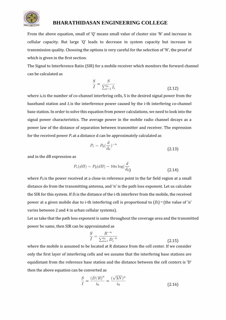
BHARATHIDASAN ENGINEERING COLLEGE
From the above equation, small of ‘Q’ means small value of cluster size ‘N’ and increase in
cellular capacity. But large ‘Q’ leads to decrease in system capacity but increase in
transmission quality. Choosing the options is very careful for the selection of ‘N’, the proof of
which is given in the first section.
The Signal to Interference Ratio (SIR) for a mobile receiver which monitors the forward channel
can be calculated as
(2.12)
where i0 is the number of co-channel interfering cells, S is the desired signal power from the
baseband station and Ii is the interference power caused by the i-th interfering co-channel
base station. In order to solve this equation from power calculations, we need to look into the
signal power characteristics. The average power in the mobile radio channel decays as a
power law of the distance of separation between transmitter and receiver. The expression
for the received power Pr at a distance d can be approximately calculated as
(2.13)
and in the dB expression as
) (2.14)
where P0 is the power received at a close-in reference point in the far field region at a small
distance do from the transmitting antenna, and ‘n’ is the path loss exponent. Let us calculate
the SIR for this system. If Di is the distance of the i-th interferer from the mobile, the received
power at a given mobile due to i-th interfering cell is proportional to (Di)−n (the value of ’n’
varies between 2 and 4 in urban cellular systems).
Let us take that the path loss exponent is same throughout the coverage area and the transmitted
power be same, then SIR can be approximated as
(2.15)
where the mobile is assumed to be located at R distance from the cell center. If we consider
only the first layer of interfering cells and we assume that the interfering base stations are
equidistant from the reference base station and the distance between the cell centers is ’D’
then the above equation can be converted as
(2.16)

BHARATHIDASAN ENGINEERING COLLEGE
which is an approximate measure of the SIR. Subjective tests performed on AMPS cellular
system which uses FM and 30 kHz channels show that sufficient voice quality can be obtained
by SIR being greater than or equal to 18 dB. If we take n=4 , the value of ’N’ can be calculated
as 6.49. Therefore minimum N is 7. The above equations are based on hexagonal geometry
and the distances from the closest interfering cells can vary if different frequency reuse plans
are used.
We can go for a more approximate calculation for co-channel SIR. This is the example of a 7
cell reuse case. The mobile is at a distance of D-R from 2 closest interfering cells and
approximately D+R/2, D, D-R/2 and D+R distance from other interfering cells in the first tier.
Taking n = 4 in the above equation, SIR can be approximately calculated as
which can be rewritten in terms frequency reuse ratio Q as
. (2.18)
Using the value of N equal to 7 (this means Q = 4.6), the above expression yields that worst
case SIR is 53.70 (17.3 dB). This shows that for a 7 cell reuse case the worst case SIR is slightly
less than 18 dB. The worst case is when the mobile is at the corner of the cell i.e., on a vertex
as shown in the Figure 3.6. Therefore N = 12 cluster size should be used. But this reduces the
capacity by 7/12 times. Therefore, co-channel interference controls link performance, which
in a way controls frequency reuse plan and the overall capacity of the cellular system. The
effect of co-channel interference can be minimized by optimizing the frequency assignments
of the base stations and their transmit powers. Tilting the base-station antenna to limit the
spread of the signals in the system can also be done.

BHARATHIDASAN ENGINEERING COLLEGE
Figure : First tier of co-channel interfering cells
2.9.2 Adjacent Channel Interference (ACI)
This is a different type of interference which is caused by adjacent channels i.e. channels in
adjacent cells. It is the signal impairment which occurs to one frequency due to presence of
another signal on a nearby frequency. This occurs when imperfect receiver filters allow
nearby frequencies to leak into the passband. This problem is enhanced if the adjacent
channel user is transmitting in a close range compared to the subscriber’s receiver while the
receiver attempts to receive a base station on the channel. This is called near-far effect. The
more adjacent channels are packed into the channel block, the higher the spectral efficiency,
provided that the performance degradation can be tolerated in the system link budget. This
effect can also occur if a mobile close to a base station transmits on a channel close to one
being used by a weak mobile. This problem might occur if the base station has problem in
discriminating the mobile user from the ”bleed over” caused by the close adjacent channel
mobile.
Adjacent channel interference occurs more frequently in small cell clusters and heavily used
cells. If the frequency separation between the channels is kept large this interference can be
reduced to some extent. Thus assignment of channels is given such that they do not form a
contiguous band of frequencies within a particular cell and frequency separation is
maximized. Efficient assignment strategies are very much important in making the

BHARATHIDASAN ENGINEERING COLLEGE
interference as less as possible. If the frequency factor is small then distance between the
adjacent channels cannot put the interference level within tolerance limits. If a mobile is 10
times close to the base station than other mobile and has energy spill out of its passband, then
SIR for weak mobile is approximately
(2.19)
which can be easily found from the earlier SIR expressions. If n = 4, then SIR is −52 dB. Perfect
base station filters are needed when close-in and distant users share the same cell. Practically,
each base station receiver is preceded by a high Q cavity filter in order to remove adjacent
channel interference. Power control is also very much important for the prolonging of the
battery life for the subscriber unit but also reduces reverse channel SIR in the system. Power
control is done such that each mobile transmits the lowest power required to maintain a good
quality link on the reverse channel.
2.10 Enhancing Capacity And Cell Coverage
2.10.1 The Key Trade-off
Previously, we have seen that the frequency reuse technique in cellular systems allows for
almost boundless expansion of geographical area and the number of mobile system users
who could be accommodated. In designing a cellular layout, the two
parameters which are of great significance are the cell radius R and the cluster size
√
N, and we have also seen that co-channel cell distance D = 3NR. In the following, a brief
description of the design trade-off is given, in which the above two parameters play a crucial
role.
The cell radius governs both the geographical area covered by a cell and also the number of
subscribers who can be serviced, given the subscriber density. It is easy to see that the cell
radius must be as large as possible. This is because, every cell requires an investment in a
tower, land on which the tower is placed, and radio transmission equipment and so a large
cell size minimizes the cost per subscriber.
Eventually, the cell radius is determined by the requirement that adequate signal to noise
ratio be maintained over the coverage area. The SNR is determined by several factors such as

BHARATHIDASAN ENGINEERING COLLEGE
the antenna height, transmitter power, receiver noise figure etc. Given a cell radius R and a
cluster size N, the geographic area covered by a
cluster is
√
Acluster = NAcell = N3 3R2/2. (2.20)
If the total serviced area is Atotal, then the number of clusters M that could be accommodated is
given by
√
M = Atotal/Acluster = Atotal/(N3 3R2/2). (2.21)
Note that all of the available channels N, are reused in every cluster. Hence, to make the
maximum number of channels available to subscribers, the number of clusters M should be
large, which, by Equation (3.21), shows that the cell radius should be small. However, cell
radius is determined by a trade-off: R should be as large as possible to minimize the cost of
the installation per subscriber, but R should be as small as possible to maximize the number
of customers that the system can accommodate. Now, if the cell radius R is fixed, then the
number of clusters could be maximized by minimizing the size of a cluster N. We have seen
earlier that the size of a cluster depends on the frequency reuse ratio Q. Hence, in determining
the value of N, another trade-off is encountered in that N must be small to accommodate large
number of subscribers, but should be sufficiently large so as to minimize the
interference effects.
Now, we focus on the issues regarding system expansion. The history of cellular phones has
been characterized by a rapid growth and expansion in cell subscribers. Though a cellular
system can be expanded by simply adding cells to the geographical area, the way in which
user density can be increased is also important to look at. This is because it is not always
possible to counter the increasing demand for cellular systems just by increasing the
geographical coverage area due to the limitations in obtaining new land with suitable
requirements. We discuss here two methods for dealing with an increasing subscriber
density: Cell Splitting and Sectoring. The other method, microcell zone concept can treated as
enhancing the QoS in a cellular system.
The basic idea of adopting the cellular approach is to allow space for the growth of mobile
users. When a new system is deployed, the demand for it is fairly low and users are assumed
to be uniformly distributed over the service area. However, as new users subscribe to the
cellular service, the demand for channels may begin to exceed the capacity of some base

BHARATHIDASAN ENGINEERING COLLEGE
stations. As discussed previously,the number of channels available to customers
(equivalently, the channel density per square kilometer) could be increased by decreasing
the cluster size. However, once a system has been initially deployed, a system-wide reduction
in cluster size may not be necessary since user density does not grow uniformly in all parts
of the geographical area. It might be that an increase in channel density is required only in
specific parts of the system to support an increased demand in those areas. Cell-splitting is a
technique which has the capability to add new smaller cells in specific areas of the system.
2.10.2 Cell-Splitting
Cell Splitting is based on the cell radius reduction and minimizes the need to modify the
existing cell parameters. Cell splitting involves the process of sub-dividing a congested cell
into smaller cells, each with its own base station and a corresponding reduction in antenna
size and transmitting power. This increases the capacity of a cellular system since it increases
the number of times that channels are reused. Since the new cells have smaller radii than the
existing cells, inserting these smaller cells, known as microcells, between the already existing
cells results in an increase of capacity due to the additional number of channels per unit area.
There are few challenges in increasing the capacity by reducing the cell radius. Clearly, if cells
are small, there would have to be more of them and so additional base stations will be needed
in the system. The challenge in this case is to introduce the new base stations without the
need to move the already existing base station towers. The other challenge is to meet the
generally increasing demand that may vary quite rapidly between geographical areas of the
system. For instance, a city may have highly populated areas and so the demand must be
supported by cells with the smallest radius. The radius of cells will generally increase as we
move from urban to sub urban areas, because the user density decreases on moving towards
sub-urban areas. The key factor is to add as minimum number of smaller cells as possible

BHARATHIDASAN ENGINEERING COLLEGE
Figure : Splitting of congested seven-cell clusters.
wherever an increase in demand occurs. The gradual addition of the smaller cells implies that,
at least for a time, the cellular system operates with cells of more than one size.
Figure 3.7 shows a cellular layout with seven-cell clusters. Consider that the cells in the center
of the diagram are becoming congested, and cell A in the center has reached its maximum
capacity. Figure also shows how the smaller cells are being superimposed on the original
layout. The new smaller cells have half the cell radius of the original cells. At half the radius,
the new cells will have one-fourth of the area and will consequently need to support one-
fourth the number of subscribers. Notice that one of the new smaller cells lies in the center of
each of the larger cells. If we assume that base stations are located in the cell centers, this
allows the original base stations to be maintained even in the new system layout. However,
new base stations will have to be added for new cells that do not lie in the center of the larger
cells. The organization of cells into clusters is independent of the cell radius, so that the
cluster size can be the same in the small-cell layout as it was in the large-cell layout. Also the
signal-to-interference ratio is determined by cluster size and not by cell radius. Consequently,
if the cluster size is maintained, the signal-to-interference ratio will be the same after cell
splitting as it was before. If the entire system is replaced with new half-radius cells, and the
cluster size is maintained, the number of channels per cell will be exactly as it was before, and
the number of subscribers per cell will have been reduced.

BHARATHIDASAN ENGINEERING COLLEGE
When the cell radius is reduced by a factor, it is also desirable to reduce the transmitted
power. The transmit power of the new cells with radius half that of the old cells can be found
by examining the received power PR at the new and old cell boundaries and setting them
equal. This is necessary to maintain the same frequency re-use plan in the new cell layout as
well. Assume that PT1 and PT2 are the transmit powers of the larger and smaller base
stations respectively. Then, assuming a path loss index n=4, we have power received at old
cell boundary = PT1/R4 and the power received at new cell boundary = PT2/(R/2)4. On equating
the two received powers, we get PT2 = PT1 / 16. In other words, the transmit power must be
reduced by 12 dB in order to maintain the same S/I with the new system lay-out.
At the beginning of this channel splitting process, there would be fewer channels in the
smaller power groups. As the demand increases, more and more channels need to be
accommodated and hence the splitting process continues until all the larger cells have been
replaced by the smaller cells, at which point splitting is complete within the region and the
entire system is rescaled to have a smaller radius per cell.
If a cellular layout is replaced entirety by a new layout with a smaller cell radius, the signal-
to-interference ratio will not change, provided the cluster size does not change. Some special
care must be taken, however, to avoid co-channel interference when both large and small cell
radii coexist. It turns out that the only way to avoid interference between the large-cell and
small-cell systems is to assign entirely different sets of channels to the two systems. So, when
two sizes of cells co-exist in a system, channels in the old cell must be broken down into two
groups, one that corresponds to larger cell reuse requirements and the other which
corresponds to the smaller cell reuse requirements. The larger cell is usually dedicated to
high speed users as in the umbrella cell approach so as to minimize the number of hand-offs.
Ex. 4: When the AMPS cellular system was first deployed, the aim of the system designers was
to guarantee coverage. Initially the number of users was not significant. Consequently cells
were configured with an eight-mile radius, and a
12-cell cluster size was chosen. The cell radius was chosen to guarantee a 17 dB

BHARATHIDASAN ENGINEERING COLLEGE
Figure : A cell divided into three 120o sectors.
signal-to-noise ratio over 90% of the coverage area. Although a 12-cell cluster size provided
more than adequate co-channel separation to meet a requirement for a 17 dB signal-to-
interference ratio in an interference-limited environment, it did not provide adequate
frequency reuse to service an explosively growing customer base. The system planners
reasoned that a subsequent shift to a 7-cell cluster size would provide an adequate number
of channels. It was estimated that a 7-cell cluster size should provide an adequate 18.7 dB
signal-to-interference ratio. The margin, however, is slim, and the 17 dB signal-to-
interference ratio requirement could not be met over 90 % of the coverage area.
2.10.3 Sectoring
Sectoring is basically a technique which can increase the SIR without necessitating an
increase in the cluster size. Till now, it has been assumed that the base station is located in
the center of a cell and radiates uniformly in all the directions behaving as an omni-
directional antenna. However it has been found that the co-channel interference in a cellular
system may be decreased by replacing a single omni-directional antenna at the base station
by several directional antennas, each radiating within a specified sector. In the Figure 3.8, a
cell is shown which has been split into three 120o sectors. The base station feeds three 120o
directional antennas, each of which radiates into one of the three sectors. The channel set
serving this cell has also been divided, so that each sector is assigned one-third of the
available number cell of channels. This technique for reducing co-channel interference
wherein by using suit-
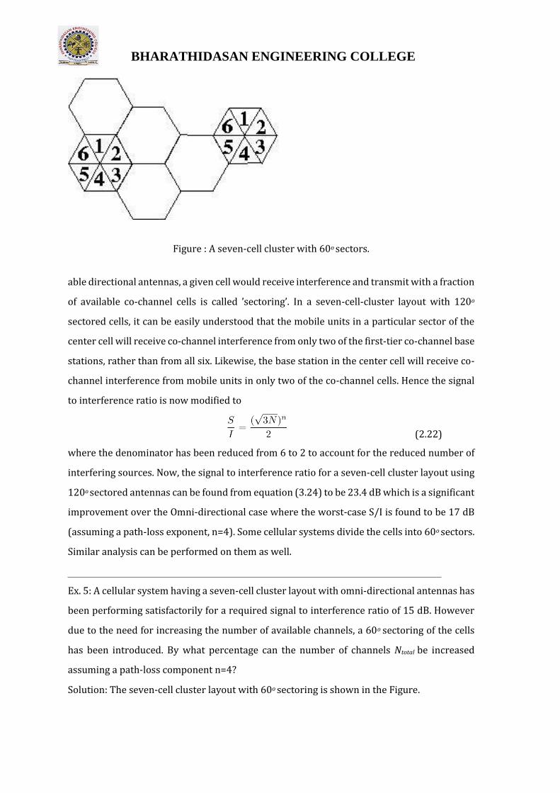
BHARATHIDASAN ENGINEERING COLLEGE
Figure : A seven-cell cluster with 60o sectors.
able directional antennas, a given cell would receive interference and transmit with a fraction
of available co-channel cells is called ’sectoring’. In a seven-cell-cluster layout with 120o
sectored cells, it can be easily understood that the mobile units in a particular sector of the
center cell will receive co-channel interference from only two of the first-tier co-channel base
stations, rather than from all six. Likewise, the base station in the center cell will receive co-
channel interference from mobile units in only two of the co-channel cells. Hence the signal
to interference ratio is now modified to
(2.22)
where the denominator has been reduced from 6 to 2 to account for the reduced number of
interfering sources. Now, the signal to interference ratio for a seven-cell cluster layout using
120o sectored antennas can be found from equation (3.24) to be 23.4 dB which is a significant
improvement over the Omni-directional case where the worst-case S/I is found to be 17 dB
(assuming a path-loss exponent, n=4). Some cellular systems divide the cells into 60o sectors.
Similar analysis can be performed on them as well.
Ex. 5: A cellular system having a seven-cell cluster layout with omni-directional antennas has
been performing satisfactorily for a required signal to interference ratio of 15 dB. However
due to the need for increasing the number of available channels, a 60o sectoring of the cells
has been introduced. By what percentage can the number of channels Ntotal be increased
assuming a path-loss component n=4?
Solution: The seven-cell cluster layout with 60o sectoring is shown in the Figure.

BHARATHIDASAN ENGINEERING COLLEGE
It is easy to see that the shaded region in the center receives interference from just one first-
tier cell and hence the signal to interference ratio can be obtained suitably as
(2.23)
Since the SIR exceeds 15 dB, one can try reducing the cluster size from seven to four. Now, the
SIR for this reduced cluster size layout can be found to be
(2.24)
The S/I ratio is still above the requirement and so a further reduction in the cell cluster size
is possible. For a 3-cell cluster layout, there are two interfering sources and hence the S/I
ratio is found to be
(2.25)
This is just above the adequate S/I ratio and further reduction in cluster size is not possible.
So, a 3-cluster cell layout could be used for meeting the growth requirements. Thus, when the
cluster size is reduced from 7 to 3, the total number of channels increased by a factor of 7/3.
The calculations in the above example are actually an idealization for several reasons. Firstly,
practical antennas have side lobes and cannot be used to focus a transmitted beam into a
perfect 120o sector or 60o sector. Due to this, additional interference will be introduced. Next,
it is also a cause of concern that a given number of channels are not able to support as many
subscribers when the pool of channels is divided into small groups. This is due to a reduction
in Trunking Efficiency, a term which will be explained later on. Because sectoring involves
using more than one antenna per base station, the available channels in the cell are divided
and dedicated to a specific antenna. This breaks the available set of channels into smaller sets,
thus reducing the trunking efficiency. Moreover, dividing a cell into sectors requires that a
call in progress will have to be handed off (that is, assigned a new channel) when a mobile
unit travels into a new sector. This increases the complexity of the system and also the load
on the mobile switching center/base
station.
2.10.4 Microcell Zone Concept
The increased number of handoffs required when sectoring is employed results in an
increased load on the switching and control link elements of the mobile system. To overcome

BHARATHIDASAN ENGINEERING COLLEGE
this problem, a new microcell zone concept has been proposed. As shown in Figure, this
scheme has a cell divided into three microcell zones, with each of the three zone sites
connected to the base station and sharing the same radio equipment. It is necessary to note
that all the microcell zones, within a cell, use the same frequency used by that cell; that is no
handovers occur between microcells. Thus when a mobile user moves between two microcell
zones of the cell, the BS simply switches the channel to a different zone site and no physical
re-allotment of channel takes place.
Locating the mobile unit within the cell: An active mobile unit sends a signal to all
zone sites, which in turn send a signal to the BS. A zone selector at the BS uses that signal to
select a suitable zone to serve the mobile unit - choosing the zone with the strongest signal.
Base Station Signals: When a call is made to a cellular phone, the system already
knows the cell location of that phone. The base station of that cell knows in which zone, within
that cell, the cellular phone is located. Therefore when it receives the signal, the base station
transmits it to the suitable zone site. The zone site receives the cellular signal from the base
station and transmits that signal to the mobile phone after amplification. By confining the
power transmitted to the mobile phone, co-channel interference is reduced between the
zones and the capacity of system is
increased.
Benefits of the micro-cell zone concept:
1) Interference is reduced in this case as compared to the scheme in which the cell size is
reduced.
2) Handoffs are reduced (also compared to decreasing the cell size) since the microcells
within the cell operate at the same frequency; no handover occurs when the mobile unit moves
between the microcells.
3) Size of the zone apparatus is small. The zone site equipment being small can be mounted
on the side of a building or on poles.
4) System capacity is increased. The new microcell knows where to locate the mobile unit in
a particular zone of the cell and deliver the power to that zone. Since

BHARATHIDASAN ENGINEERING COLLEGE
Figure : The micro-cell zone concept.
the signal power is reduced, the microcells can be closer and result in an increased system
capacity. However, in a microcellular system, the transmitted power to a mobile phone within
a microcell has to be precise; too much power results in interference between microcells,
while with too little power the signal might not reach the mobile phone.This is a drawback of
microcellular systems, since a change in the surrounding (a new building, say, within a
microcell) will require a change of the transmission power.
2.11 Trunked Radio System
In the previous sections, we have discussed the frequency reuse plan, the design trade-offs
and also explored certain capacity expansion techniques like cell-splitting and sectoring.
Now, we look at the relation between the number of radio channels a cell contains and the
number of users a cell can support. Cellular systems use the concept of trunking to
accommodate a large number of users in a limited radio spectrum. It was found that a central
office associated with say, 10,000 telephones requires about 50 million connections to
connect every possible pair of users. However, a worst case maximum of 5000 connections
need to be made among these telephones at any given instant of time, as against the possible

BHARATHIDASAN ENGINEERING COLLEGE
50 million connections. In fact, only a few hundreds of lines are needed owing to the relatively
short duration of a call. This indicates that the resources are shared so that the number of
lines is much smaller than the number of possible connections. A line that connects switching
offices and that is shared among users on an as-needed basis is called a trunk.
The fact that the number of trunks needed to make connections between offices is much
smaller than the maximum number that could be used suggests that at times there might not
be sufficient facilities to allow a call to be completed. A call that cannot be completed owing
to a lack of resources is said to be blocked. So one important to be answered in mobile cellular
systems is: How many channels per cell are needed in a cellular telephone system to ensure
a reasonably low probability that a call will be blocked?
In a trunked radio system, a channel is allotted on per call basis. The performance of a radio
system can be estimated in a way by looking at how efficiently the calls are getting connected
and also how they are being maintained at handoffs.
Some of the important factors to take into consideration are (i) Arrival statistics, (ii)Service
statistics, (iii)Number of servers/channels.
Let us now consider the following assumptions for a bufferless system handling ’L’ users as
shown in Figure:
(i) The number of users L is large when compared to 1.
(ii) Arrival statistics is Poisson distributed with a mean parameter λ.
(iii) Duration of a call is exponentially distributed with a mean rate µ1. (iv) Residence time of each
user is exponentially distributed with a rate parameter
µ2.
(v) The channel holding rate therefore is exponentially distributed with a parameter
µ = µ1 + µ2.
(vi) There is a total of ’J’ number of channels (J ≤ L).
To analyze such a system, let us recapitulate a queuing system in brief. Consider an
M/M/m/m system which is an m-server loss system. The name M/M/m/m reflects
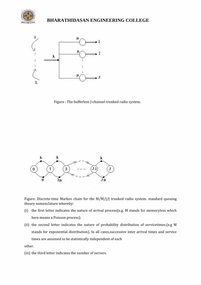
BHARATHIDASAN ENGINEERING COLLEGE
Figure : The bufferless J-channel trunked radio system.
Figure: Discrete-time Markov chain for the M/M/J/J trunked radio system. standard queuing
theory nomenclature whereby:
(i) the first letter indicates the nature of arrival process(e.g. M stands for memoryless which
here means a Poisson process).
(ii) the second letter indicates the nature of probability distribution of servicetimes.(e.g M
stands for exponential distribution). In all cases,successive inter arrival times and service
times are assumed to be statistically independent of each
other.
(iii) the third letter indicates the number of servers.

BHARATHIDASAN ENGINEERING COLLEGE
(iv) the last letter indicates that if an arrival finds all ’m’ users to be busy, then itwill not enter
the system and is lost.
In view of the above, the bufferless system as shown in Figure can be modeled as M/M/J/J
system and the discrete-time Markov chain of this system is shown in Figure.
Trunking mainly exploits the statistical behavior of users so that a fixed number of channels
can be used to accommodate a large, random user community. As the number of telephone
lines decrease, it becomes more likely that all channels are busy for a particular user. As a
result, the call gets rejected and in some systems, a queue may be used to hold the caller’s
request until a channel becomes available. In the telephone system context the term Grade of
Service (GoS) is used to mean the probability that a user’s request for service will be blocked
because a required facility, such as a trunk or a cellular channel, is not available. For example,
a GoS of 2 % implies that on the average a user might not be successful in placing a call on 2
out of every 100 attempts. In practice the blocking frequency varies with time. One would
expect far more call attempts during business hours than during the middle of the night.
Telephone operating companies maintain usage records and can identify a ”busy hour”, that
is, the hour of the day during which there is the greatest demand for service. Typically,
telephone systems are engineered to provide a specified grade of service during a specified
busy hour.
User calling can be modeled statistically by two parameters: the average number of call
requests per unit time λuser and the average holding time H. The parameter λuser is also called
the average arrival rate, referring to the rate at which calls from a single user arrive. The
average holding time is the average duration of a call. The product:
Auser = λuserH (2.26)
that is, the product of the average arrival rate and the average holding time–is called the
offered traffic intensity or offered load. This quantity represents the average traffic that a
user provides to the system. Offered traffic intensity is a quantity that is traditionally
measured in Erlangs. One Erlang represents the amount of traffic intensity carried by a
channel that is completely occupied. For example, a channel that is occupied for thirty
minutes during an hour carries 0.5 Erlang of traffic.
Call arrivals or requests for service are modeled as a Poisson random process. It is based on
the assumption that there is a large pool of users who do not cooperate in deciding when to
place calls. Holding times are very well predicted using an exponential probability

BHARATHIDASAN ENGINEERING COLLEGE
distribution. This implies that calls of long duration are much less frequent than short calls.
If the traffic intensity offered by a single user is Auser, then the traffic intensity offered by N
users is A = NAuser. The purpose of the statistical model is to relate the offered traffic intensity
A, the grade of service Pb, and the number of channels or trunks C needed to maintain the
desired grade
of service.
Two models are widely used in traffic engineering to represent what happens when a call is
blocked. The blocked calls cleared model assumes that when a channel or trunk is not
available to service an arriving call, the call is cleared from the system. The second model is
known as blocked calls delayed. In this model a call that cannot be serviced is placed on a
queue and will be serviced when a channel or trunk becomes available.
Use of the blocked-calls-cleared statistical model leads to the Erlang B formula that relates
offered traffic intensity A, grade of service Pb, and number of channels K. The Erlang B formula
is:
(3.27)
!
When the blocked-calls-delayed model is used, the ”grade of service” refers to the probability that
a call will be delayed. In this case the statistical model leads to the
Erlang C formula,
. (2.28)
Ex. 6: In a certain cellular system, an average subscriber places two calls per hour during a
busy hour and the average holding time is 3 min. Each cell has 100 channels. If the blocked
calls are cleared, how many subscribers can be serviced by each cell at 2 % GoS?
Solution: Using Erlang B table, it can be seen that for C = 100 and GoS = Pb = 2%, the total
offered load A=87.972 Erlangs. Since an individual subscriber offers a load of Auser = (2 calls /
60 min)3 min = 0.1 Erlang, the maximum number of subscribers served is
N = A/Auser = 87.972/0.1 ≈ 880. (2.29)
Ex. 4: In the previous example, suppose that the channels have been divided into two groups
of 50 channels each. Each subscriber is assigned to a group and can be served only by that
group. How many subscribers can be served by the two group
cell?

BHARATHIDASAN ENGINEERING COLLEGE
Solution: Using the Erlang B table with C = 50 and GOS = Pb = 2%, the total
offered load per group is
A = 40.255Erlangs (2.30)
Thus the maximum number of users per group is
Ngroup = A/Auser ≈ 403. (2.31)
Thus, counting both the groups, maximum number of users in the two group cell is 806.
The above example indicates that the number of subscribers that can be supported by a given
number of channels decreases as the pool of channels is sub-divided. We can express this in
terms of the trunking efficiency, defined as the carrier load per channel, that is,
ξ = (1 − Pb)A/C. (2.32)
This explains why the sectoring of a cell into either 120o or 60o sectors reduces the trunking
efficiency of the system. Thus the system growth due to sectoring is impacted by trunking
efficiency considerations.
2.12 References
1. T. S. Rappaport, Wireless Communications: Principles and Practice, 2nd ed. Singapore:
Pearson Education, Inc., 2002.
2. K. Feher, Wireless Digital Communications: Modulation and Spread Spectrum Applications.
Upper Saddle River, NJ: Prentice Hall, 1995.
3. S. Haykin and M. Moher, Modern Wireless Communications. Singapore: Pearson Education,
Inc., 2002.
4. J. W. Mark and W. Zhuang, Wireless Communications and Networking. New
Delhi: PHI, 2005.

BHARATHIDASAN ENGINEERING COLLEGE
UNIT III DIGITAL SIGNALING FOR FADING CHANNELS
Structure of a wireless communication link, Principles of Offset-QPSK, p/4-
DQPSK, Minimum Shift Keying, Gaussian Minimum Shift Keying, Error
performance in fading channels, OFDM principle – Cyclic prefix,
Windowing, PAPR.
3.1 Structure of a wireless communication link
The information source provides an analog source signal and feeds it into the source ADC (Analog
to Digital Converter). This ADC first band limits the signal from the analog information
source (if necessary), and then converts the signal into a stream of digital data at a certain sampling
rate and resolution (number of bits per sample). For example, speech would typically be sampled at
8ksamples/s, with 8-bit resolution, resulting in a DataStream at 64 kbit/s. For the transmission of

BHARATHIDASAN ENGINEERING COLLEGE
digital data, these steps can be omitted, and the digital source directly provides the input to interface
“G” in Figure
The source coder uses a priori information on the properties of the source data in order to
reduce redundancy in the source signal. This reduces the amount of source data to be
transmitted, and thus the required transmission time and/or bandwidth.
The channel coder adds redundancy in order to protect data against transmission errors. This
increases the data rate that has to be transmitted at interface E – e.g., GSM channel coding
increases the data rate from 13 to 22.8 kbit/s. Channel coders often use information about
the statistics of error sources in the channel (noise power, interference statistics) to design
codes that are especially well suited for certain types of channels (e.g., Reed–Solomon codes
protect especially well against burst errors).
Signaling adds control information for the establishing and ending of connections, for
associating information with the correct users, synchronization, etc. Signaling information
is usually strongly protected by error correction codes.
The multiplexer combines user data and signaling information, and combines the data from
multiple users.2 if this is done by time multiplexing, the multiplexing requires some time
compression.
The baseband modulator assigns the gross data bits (user data and signaling at interface D)
to complex transmit symbols in the baseband. Spectral properties, intersymbol interference,
peakto- average ratio, and other properties of the transmit signal are determined by this step.
The output from the baseband modulator (interface C) provides the transmit symbols in
oversampled form, discrete in time and amplitude. Oversampling and quantization
determine the aliasing and quantization noise. Therefore, high resolution is desirable, and
the data rate at the output of the baseband modulator should be much higher than at the
input.
The source decoder reconstructs the source signal from the rules of source coding. If the
source data are digital, the output signal is transferred to the data sink. Otherwise, the data
are transferred to the DAC, which converts the transmitted information into an analog signal,
and hands it over to the information sink.

BHARATHIDASAN ENGINEERING COLLEGE
Quadrature Phase Shift Keying (QPSK)
Quadrature phase shift keying (QPSK) has twice the bandwidth efficiency of BPSK, since 2 bits are
transmitted in a single modulation symbol. The phase of the carrier takes on 1 of 4 equally spaced
values, such as 0, it/2, it, and 3it/2, where each value of phase corresponds to a unique pair of
message bits. The QPSK signal for this set of symbol states may be defined as
SQPSK(t) = √2𝐸0
𝑇𝑠cos[2𝜋𝑓𝐶𝑡 + (ⅈ − 1)
𝜋
2] 0≤ t ≤ 𝑡𝑠 i = 1,2,3,4. … (1)
where Ts is the symbol duration and is equal to twice the bit period. Using trigonometric identities,
the above equations can be rewritten for the interval 0 < t _<Ts as,
SQPSK(t) =√2𝐸𝑠
𝑇𝑠cos[(ⅈ − 1)
𝜋
2] cos(2𝜋𝑓𝑐𝑡) −√
2𝐸𝑠
𝑇𝑠sin[(ⅈ − 1)
𝜋
2] sin(2𝜋𝑓𝑐𝑡) … (2)
If basis function ϕ1(t) = √2
Tscos(2Πfct) , 𝜙2(𝑡) = √
2
𝑇𝑠sin(2𝜋𝑓𝑐𝑡) are defined the interval 0≤ t ≤ 𝑡𝑠
for the QPSK signal set, then the 4 signals in the set can be expressed in terms of the basis signal
as

BHARATHIDASAN ENGINEERING COLLEGE
𝑠𝑄𝑃𝑠𝑘 = √𝐸9cos[(ⅈ − 1)𝜋
2] 𝜙1(𝑡) − √𝐸5sin[(ⅈ − 1)
𝜋
2] 𝜙2(𝑡) … (3)
Based on this representation, a QPSK signal can be depicted using a two dimensional constellation
diagram with four points. It should be noted that different QPSK signal sets can be derived by
simply rotating the constellation.
From the constellation diagram of a QPSK signal, it can be seen that the distance between adjacent
points in the constellation is Since each symbol corresponds to two bits, then E, = 2E6, thus the
distance between two neighboring points in the QPSK constellation is equal to 2, the average
probability of bit error in the additive white Gaussian noise (AWGN) channel is obtained as
𝑝𝑒,𝑄𝑃𝑠𝑘 = 𝑄 (√2𝐸𝑏
𝑁0) … (3)
A striking result is that the bit error probability of QPSK is identical to BPSK, but twice as much
data can be sent in the same bandwidth. Thus when compared to BPSK, QPSK provides twice the
spectral efficiency with exactly the same energy efficiency. Similar to BPSK QPSK can also be
differentially encoded to allow noncoherent detection.
QPSK Transmission
The unipolar binary message stream has bit rate Rb and is first converted into a bipolar non-return-
to-zero (NRZ) sequence using a unipolar to bipolar convener. The bit stream m (t) is then split into
two bit streams in1 (t) and TflQ (t) (in-phase and quadrature streams), each having a bit rate of R3
= Rb/2. The bit stream m1 (t) is called the "even" stream and mQ (t) is called the "odd" stream. The
two binary sequences are separately modulated by two carriers +i(t) and which are in quadrature.
The two modulated signals, each of which can be considered to be a BPSK signal, are summed to
produce a QPSK signal. The filter at the output of the modulator confines the power spectrum of
the QPSK signal within the allocated band.

BHARATHIDASAN ENGINEERING COLLEGE
This prevents spill-over of signal energy into adjacent channels and also removes out-of-band
spurious signals generated during the modulation process. In most implementations, pulse shaping
is done at baseband to provide proper RF filtering at the transmitter output.
QPSK Transmission and Detection Techniques
Figure shows a block diagram of a coherent QPSK receiver. The frontend bandpass filter removes
the out-of-band noise and adjacent channel interference. The filtered output is split into two parts,
and each part is coherently demodulated using the in-phase and quadrature carriers. The coherent
carriers used for demodulation are recovered from the received signal using carrier recovery circuits
of the type described in Figure. The outputs of the demodulators are passed through decision circuits
which generate the in-phase and quadrature binary streams. The two components are then
multiplexed to reproduce the original binary sequence.
Differential PSK is a noncoherent form of phase shift keying which avoids the need for a coherent
reference signal at the receiver. Noncoherent receivers are easy and cheap to build, and hence are
widely used in wireless communications. In DPSK systems, the input binary sequence is first
differentially encoded and then modulated using a BPSK modulator. The differentially encoded
sequence dk is generated from the input binary sequence I by complementing the modulo-2 sum
of mk and dk - The effect is to leave the symbol dk unchanged from the previous symbol if the
incoming binary symbol mk is 1, and to toggle dk if mk is 0.
Table 5.1 illustrates the generation of a DPSK signal for a sample sequence which follows the
relationship dk = mk e dk –

BHARATHIDASAN ENGINEERING COLLEGE
DPSK transmitter
A block diagram of a DPSK transmitter is shown in Figure. It consists of a one bit delay element
and a logic circuit interconnected so as to generate the differentially encoded sequence from the
input binary sequence. The output is passed through a product modulator to obtain the DPSK signal.
At the receiver, the original sequence is recovered from the demodulated differentially encoded
signal through a complementary process.
DPSK Receiverr
While DPSK signaling has the advantage of reduced receiver complexity, its energy efficiency is
inferior to that of coherent PSK by about 3 dB. The average probability of error for DPSK in additive
white Gaussian noise is given by
𝑃𝑒,𝐷𝑝𝑠𝑘 =1
2exp(
𝐸𝑏
𝑁0) … (1)

BHARATHIDASAN ENGINEERING COLLEGE
4. Explain with a block diagram, Offset-Quadrature Phase Shift Keying and its advantages.
(8)[M/J –12]
Offset QPSK
The amplitude of a QPSK signal is ideally constant. However, when QPSK signals are pulse shaped,
they lose the constant envelope property. The occasional phase shift of it radians can cause the
signal envelope to pass through zero for just an instant. Any kind of hard limiting or nonlinear
amplification of the zero-crossings brings back the filtered side lobes since the fidelity of the signal
at small voltage levels is lost in transmission. The prevent regeneration of side lobes and spectral
widening; it is imperative that QPSK signals be amplified only using linear amplifiers, which are
less efficient. A modified form of QPSK, called offset QPSK (OQPSK) or staggered QPSK is less
susceptible to these deleterious effects more efficient amplification. OQPSK signaling is similar to
QPSK signaling, except for the time alignment of the even and odd bit streams. In QPSK signaling,
the bit transitions of the even and odd bit streams occur at the same time instants, but in OQPSK
signaling, the even and odd bit streams, m1 (t) and are offset in theft relative alignment by one bit
period (half-symbol period). This is shown in the waveforms of Figure 5.30. Due to the time
alignment of m1 (t) and 'nq (t) in standard QPSK, phase transitions occur only once every T9 = 2Tb
s, and will be a maximum of 1800 if there is a change in the value of both m1 (t) and mQ (t)

BHARATHIDASAN ENGINEERING COLLEGE
However, in OQPSK. signaling, bit transitions (and hence phase transitions) occur every T,, s. Since
the transitions instants of ni1 (t) and mQ (t) are offset, at any given time only one of the two bit
streams can change values. This implies that the maximum phase shift of the transmitted signal at
any given time is limited to ±90° - Hence, by switching phases more frequently (i.e., every Tb s
instead of 27',, s) OQPSK signaling eliminates 180° phase transitions.
Since 180° phase transitions have been eliminated, band limiting of (i.e., pulse shaping) OQPSK
signals does not cause the signal envelope to go to zero. Obviously, there will be some amount of
IS! Caused by the band limiting process, especially at the 90 phase transition points. But the
envelope variations are considerably less, and hence hard limiting or nonlinear amplification of
OQPSK signals does not regenerate the high frequency side lobes as much as in QPSK. Thus,
spectral occupancy is significantly reduced, while permitting more efficient RF amplification. The
spectrum of an OQPSK signal is identical to that of a QPSK signal; hence both signals occupy the
same bandwidth. The staggered alignment of the even and odd bit streams does not change the
nature of the spectrum. OQPSK retains its hand limited nature even after nonlinear amplification,
and therefore ii very attractive for mobile communication systems where bandwidth efficiency and
efficient nonlinear amplifiers are critical for 1ow power drain. Further, OQPSK signals also appear
to perform better than QPSK in the presence of phase jitter due to noisy reference signals at the
receiver.
5. Explain the BPSK digital modulation scheme. S (8)
Binary Phase Shift Keying (BPSK)
In binary phase shift keying (BPSK), the phase of a constant amplitude carrier signal is switched
between two values according to the two possible signals m and rn., corresponding to binary 1 and
0, respectively. Normally, the two

BHARATHIDASAN ENGINEERING COLLEGE
𝑠𝐵𝑃𝑠𝑘(𝑡) = √2𝐸𝑏
𝑇𝑏cos(2𝜋𝑓𝐶𝑡 + 𝜃𝑐)0≤𝑡≤𝑇𝑏 0 ≤ t ≤ Tb (Binary 1) … (1)
Phases are separated by 1800. If the sinusoidal carrier has an amplitude Ac and energy per bit
𝐸𝑏 =1
2𝐴𝑐2𝑇𝑏, then the transmitted BPSK signal is either it is often convenient to generalize in1 and
m2 as a binary data signal m(t), which takes on one of two possible pulse shapes. Then the
transmitted signal may be represented as
𝑆𝐵𝑝𝑠𝑘(𝑡) = 𝑚(𝑡)√2𝐸𝑏
𝑇𝑏cos(2𝜋𝑓𝐶𝑡 + 𝜃𝑒) … (2)
𝑠𝐵𝑝𝑠𝑘(𝑡) = √2𝐸𝑏
𝑇𝑏cos(2𝜋𝑓𝐶𝑡 + 𝜋 + 𝜃𝐶) = −√
2𝐸𝑏
𝑇𝑏cos(2𝜋𝑓𝑐𝑡 + 𝜃𝑐) 0 ≤ t ≤ Tb (binary 0)
… (3)
The BPSK signal is equivalent to a double sideband suppressed carrier amplitude modulated
waveform, where cos(2πft) is applied as the carrier, and the data signal in (t) is applied as the
modulating waveform. Hence a BPSK signal. can be generated using a balanced modulator.
BPSK Receiver
If no multipath impairments are induced by the channel, the received BPSK signal Sn be expressed
as
𝑠𝐵𝑝𝑠𝑘(𝑡) = 𝑚(𝑡)√2𝐸𝑏
𝑇𝑏cos(2𝜋𝑓𝐶𝑡 + 𝜃𝐶 + 𝜃𝐶ℎ)
𝑠𝐵𝑝𝑠𝑘(𝑡) = 𝑚(𝑡)√2𝐸𝑏
𝑇𝑏cos(2𝜋𝑓𝐶𝑡 + 𝜃) … (4)

BHARATHIDASAN ENGINEERING COLLEGE
where Ɵch is the phase shift corresponding to the time delay in the channel. BPSK uses coherent or
synchronous demodulation, which requires that information about the phase and frequency of the
carrier be available at the receiver. If a low level pilot carrier signal is transmitted along with the
BPSK signal, then the carrier phase and frequency may be recovered at the receiver using a phase
locked loop (PLL). If no pilot carrier is transmitted, a Costas loop or squaring loop may be used to
synthesize the carrier phase and frequency from the received BPSK signal. The block diagram of a
BPSK receiver along with the carrier recovery circuits is shows.
The received signal cos(2πfct + Ɵ) is squared to generate a dc signal and an amplitude varying
sinusoidal at twice the carrier frequency. The dc signal is filtered out using a bandpass filterwith
center frequency tuned to 2fc. A frequency driver is then used to recreate the waveform cos(2πfct
+ Ɵ). The output of the multiplier after the frequency divider is given by
𝑚(𝑡)√2𝐸𝑏
𝑇𝑏cos2(2𝜋𝑓𝐶𝑡 + 𝜃) = 𝑚(𝑡)√
2𝐸𝑏
𝑇𝑏[1
2+
1
2cos2(2𝜋𝑓𝑐𝑡 + 𝜃)] … (5)
This signal is applied to an integrate and dump circuit which forms the low pass filter segment of a
BPSK detector. If the transmitter and receiver pulse shapes are attached, then the detection will be
optimum. A bit synchronizer is used to facilitate sampling of the integrator output at the end of each
bit period. At the end of each bit period, the witch at the output of the integrator closes to dump the
output signal to the decision circuit. Depending on whether the integrator output is above or below
a certain threshold, the decision circuit decides that the received signal corresponds to a binary 1 or
0. The threshold is set at an optimum level such that the probability of error is minimized. If it is
equally likely that a binary 1 or 0 is transmitted, then the voltage level corresponding to the midpoint
between the detector output voltage levels of binary 1 and 0 is used as the optimum threshold.
The probability of bit error for many modulation schemes in an AWGN channel is found using the
Q-function of the distance between the signal points. From the constellation diagram of a BPSK

BHARATHIDASAN ENGINEERING COLLEGE
signal shown in Figure 5.21, it can be seen that the distance between adjacent points in the
constellation is 2 Substituting this in equation, the probability of bit error is obtained as
𝑃𝑒,𝐵𝑝𝑠𝑘 = 𝑄 (√2𝐸𝑏
𝑁0) … (6)
6. What is BFSK? Derive the bit error probability of BFSK and also explain with its constellation
diagram. (16)
Binary Frequency Shift Keying
In binary frequency shift keying (BFSK), the frequency of a constant amplitude carrier signal is
switched between two values according to the two possible message states (called high and low
tones), corresponding to a binary 1 or 0. Depending on how the frequency variations are imparted
into the transmitted waveform, the FSK signal will have either a discontinuous phase or continuous
phase between bits. In general, an FSK signal may be represented as where 2ltêsf is a
𝑠𝐹𝑠𝑘(𝑡) = 𝑣𝐻(𝑡) = √2𝐸𝑏
𝑇𝑏cos(2𝜋𝑓𝑐 + 2𝜋𝛥𝑓)𝑡 0 ≤ t ≤ Tb (binary 1) … (1)
𝑠𝐹𝑠𝑘(𝑡) = 𝑣𝐿(𝑡) = √2𝐸𝑏
𝑇𝑏cos(2𝜋𝑓𝑐 − 2𝜋𝛥𝑓)𝑡 0 ≤ t ≤ Tb (binary 0) … (2)
constant offset from the terminal carrier frequency. One obvious way to generate an FSK signal is
to switch between two independent oscillators according to whether the data bit is a 0 or a 1.
Normally, this form of FSK generation results in a waveform that is discontinuous at the switching
times, arid for this reason this type of FSK is called discontinuous FSK. A discontinuous FSK signal
is represented as
𝑠𝐹𝑠𝑘(𝑡) = 𝑣𝐻(𝑡) = √2𝐸𝑏
𝑇𝑏cos(2𝜋𝑓𝐻𝑡 + 𝜃1) 0 ≤ t ≤ Tb (binary 1) … (3)
𝑠𝐹𝑠𝑘(𝑡) = 𝑣𝐿(𝑡) = √2𝐸𝑏
𝑇𝑏cos(2𝜋𝑓𝐿𝑡 + 𝜃2) 0 ≤ t ≤ Tb (binary 0) … (4)
Since the phase discontinuities pose several problems, such as spectral spreading and spurious
transmissions, this type of FSK is generally not used in highly regulated wireless systems. The more
common method for generating an FSK signal is to frequency modulate a single carrier oscillator
using the message waveform. This type of modulation is similar to analog FM generation, except
that the modulating signal m (t) is a binary waveform. Therefore, FSK may be represented as b
𝑠𝐹𝑆𝑘(𝑡) = √2𝐸𝑏
𝑇𝑏cos[2𝜋𝑓𝑐𝑡 + 𝜃(𝑡)] = √
2𝐸𝑏
𝑇𝑏cos[2𝜋𝑓𝑐𝑡 + 2𝜋𝑘𝑓 ∫ 𝑚(𝜂) ⅆ𝜂
𝑡
−𝛼] … (5)
It should be noted that even though the modulating waveform m (t) is discontinuous at bit
transitions, the phase function e (t) is proportional to the integral of m (t) and is continuous.
Coherent Detection of Binary FSK: A block diagram of a coherent detection scheme for
demodulation of binary FSK signals is shown in Figure. The receiver shown is the optimum detector

BHARATHIDASAN ENGINEERING COLLEGE
for coherent binary FSK in the presence of additive white Gaussian noise. It consists of two
correlators which are supplied with locally generated coherent reference signals. The difference of
the correlator outputs is then compared with a threshold comparator. If the difference signal has a
value greater than the threshold, the receiver decides in favor of a 1, otherwise it decides in favor
of a 0. It can be shown that the probability of error for a coherent FSK receiver is given by
𝑃𝑒,𝐹𝑠𝑘 = 𝑄 (√𝐸𝑏
𝑁0) … (6)
Coherent detection of FSK signal
Nohcoherent Detection of Binary FSK
Unlike phase-shift keying, it is possible to detect FSK signals in the pitsence of noise without using
a coherent carrier reference. A block diagram of a noncoherent FSK receiver is shown in Figure
5.37. The receiver consists of a pair of matched filters followed by envelope detectors. The filter in
the upper path is matched to the FSK signal of frequency and the filter in the lower path is matched
to the signal of frequency fL• These matched filters function as bandpass filters centered at and IL'
respectively. The outputs of the envelope detectors are sampled at every I = kTb, where k is an
integer, and their values compared. Depending on the magnitude of the envelope detector output,
the comparator decides whether the data bit was a 1 or 0. The average
probability of error of an FSK system employing noncoherent detection is given by
𝑃𝑒,𝐹𝑠𝑘,𝑁𝑐 =1
2exp(−
𝐸𝑏
2𝑣0) … (7)
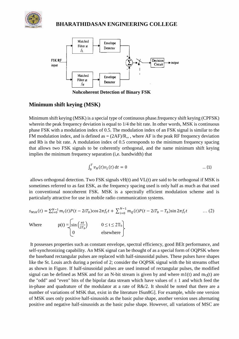
BHARATHIDASAN ENGINEERING COLLEGE
Nohcoherent Detection of Binary FSK
Minimum shift keying (MSK)
Minimum shift keying (MSK) is a special type of continuous phase.frequency shift keying (CPFSK)
wherein the peak frequency deviation is equal to 1/4 the bit rate. In other words, MSK is continuous
phase FSK with a modulation index of 0.5. The modulation index of an FSK signal is similar to the
FM modulation index, and is defined as = (2AF)/R,, , where AF is the peak RF frequency deviation
and Rb is the bit rate. A modulation index of 0.5 corresponds to the minimum frequency spacing
that allows two FSK signals to be coherently orthogonal, and the name minimum shift keying
implies the minimum frequency separation (i,e. bandwidth) that
∫ 𝑣𝐻(𝑡)𝑣𝐿(𝑡) ⅆ𝑡𝑇
0= 0 … (1)
allows orthogonal detection. Two FSK signals vH(t) and VL(t) are said to be orthogonal if MSK is
sometimes referred to as fast ESK, as the frequency spacing used is only half as much as that used
in conventional noncoherent FSK. MSK is a spectrally efficient modulation scheme and is
particularly attractive for use in mobile radio communication systems.
𝑠𝑀𝑠𝑘(𝑡) = ∑ 𝑚𝐼(𝑡)𝑃(𝑡 − 2ⅈ𝑇𝑏)cos2𝜋𝑓𝑐𝑡𝑁−1𝑖=0 +∑ 𝑚𝑄(𝑡)𝑃(𝑡 − 2ⅈ𝑇𝑏 − 𝑇𝑏)sin2𝜋𝑓𝑐𝑡
𝑁−1
𝑖=0 … (2)
Where p(t) = sin(𝜋𝑡
2𝑇𝑏) 0 ≤ t ≤ 2Tb
0 elsewhere
It possesses properties such as constant envelope, spectral efficiency, good BElt performance, and
self-synchronizing capability. An MSK signal can be thought of as a special form of OQPSK where
the baseband rectangular pulses are replaced with half-sinusoidal pulses. These pulses have shapes
like the St. Louis arch during a period of 2; consider the OQPSK signal with the bit streams offset
as shown in Figure. If half-sinusoidal pulses are used instead of rectangular pulses, the modified
signal can be defined as MSK and for an N-bit stream is given by and where m1(t) and mQ(t) are
the "odd" and "even" bits of the bipolar data stream which have values of ± 1 and which feed the
in-phase and quadrature of the modulator at a rate of R&/2. It should be noted that there are a
number of variations of MSK that, exist in the literature ISun8G]. For example, while one version
of MSK uses only positive half-sinusoids as the basic pulse shape, another version uses alternating
positive and negative half-sinusoids as the basic pulse shape. However, all variations of MSC are

BHARATHIDASAN ENGINEERING COLLEGE
continuous phase FSK employing different techniques to achieve spectral efficiency. The MSK
waveform can be seen as a special type of a continuous phase FSK is rewritten using trigonometric
identities as
𝑠𝑀𝑠𝑘(𝑡) = √2𝐸𝑏
𝑇𝑏cos2𝜋𝑓𝑐𝑡 −𝑚𝐼(𝑡)𝑚𝑄(𝑡)
𝜋𝑡
2𝑇𝑏+ 𝜙𝑘 … (3)
where 4k is 0 or it depending on whether rn1(t) is 1 or -1. From equation (2) it can be deduced that
MSK has constant amplitude. Phase continuity at the bit transition periods is ensured by choosing
the carrier frequency to be an integral multiple of one fourth the bit rate, I /4T. Comparing equation,
it can be concluded that the MSK signal is an FSK signal with binary signaling frequencies of f, —
1/4T. It can further be seen from equation (3) that the phase of the MSK signal varies linearly during
the course of each bit period
MSK Transmitter and Receiver
A special case of CPFSK is achieved with h = 0.5, and the resulting scheme is called Minimum
Shift Keying (MSK) which is used in mobile communications. In this case, the phase differences
reduce to only ±π/2 and the phase tree is called the phase trellis. An MSK signal can also be
thought as a special case of OQPSK where the baseband rectangular pulses are replaced by half
sinusoidal pulses. Spectral characteristics of an MSK signal is shown in Figure 6.9 from which it
is clear that ACI is present in the spectrum. Hence a pulse shaping technique is required. In order
to have a compact signal spectrum as well as maintaining the constant envelope property, we use
a pulse shaping filter with
Phase tree of 1101000 CPFSK sequence.

BHARATHIDASAN ENGINEERING COLLEGE
Figure: Spectrum of MSK
1. a narrow BW frequency and sharp cutoff characteristics (in order to suppressthe high
frequency component of the signal);
2. an impulse response with relatively low overshoot (to limit FM instant frequency
deviation;
3. a phase trellis with ±π/2 for odd T and 0 or π values for even T.
GMSK Scheme
GMSK is a simple modulation scheme that may be taken as a derivative of MSK.
In GMSK, the sidelobe levels of the spectrum are further reduced by passing a non-
Figure : GMSK generation scheme.

BHARATHIDASAN ENGINEERING COLLEGE
return to zero (NRZ-L) data waveform through a premodulation Gaussian pulse shaping filter.
Baseband Gaussian pulse shaping smoothes the trajectory of the MSK signals and hence stabilizes
instantaneous frequency variations over time. This has the effect of considerably reducing the
sidelobes in the transmitted spectrum. A GMSK generation scheme with NRZ-L data is shown in
Figure 6.10 and a receiver of the same scheme with some MSI gates is shown in Figure 6.11.
GMSK Generator
The GMSK premodulation filter has characteristic equation given by
H(f) = exp(−(ln2/2)(f/B)2)
H(f) = exp(−(αf)2)
where,
(6.49)
(α)2 = ln2/2(1/B)2. (6.50) The premodulation Gaussian filtering introduces ISI in the transmitted signal, but it can be shown
that the degradation is not that great if the 3dB bandwidth-bit duration product (BT) is greater
than 0.5.
Spectrum of GMSK scheme is shown in Figure 6.12. From this figure, it is evident that when
we are decreasing BT product, the out of band response decreases but
Figure : A simple GMSK receiver.

BHARATHIDASAN ENGINEERING COLLEGE
on the other hand irreducible error rate of the LPF for ISI increases. Therefore, a compromise
between these two is required.
Problem: Find the 3dB BW for a Gaussian LPF used to produce 0.25 GMSK with a channel
data rate Rb=270 kbps.What is the 90 percent power BW of the RF
filter?
Solution: From the problem statement it is clear that
T = 1/Rb = 1/270 ∗ (103) = 3.7µsec
Solving for B where BT = 0.25,
(6.51)
B = 0.25/T = 67.567kHz (6.52) Thus the 3 - dB bandwidth is 67.567 kHz. We use below table fig 6 to find out that
90 % power bandwidth is 0.57 Rb.
90 % RF BW = 0.57Rb = 153.9 kHz.
Figure 6.12: Spectrum of GMSK scheme.
Two Practical Issues of Concern
1 Inter Channel Interference
In FDMA, subscribers are allotted frequency slots called channels in a given band of the
electromagnetic spectrum. The side lobes generated due to the transmission of a symbol in a
particular channel overlaps with the channels placed adjacently. This is because of the fact that
transmission of a time limited pulse leads to spectral spreading in the frequency domain. During

BHARATHIDASAN ENGINEERING COLLEGE
simultaneous use of adjacent channels, when there is significant amount of power present in the
side lobes, this kind of interference becomes so severe that the required symbol in a particular
frequency slot is completely lost.
Moreover if two terminals transmit equal power then due to wave propagation through
different distances to the receiver, the received signal levels in the two frequency slots will differ
greatly. In such a case the side lobes of the stronger signal will severely degrade the transmitted
signal in the next frequency slot having low power level. This is known as the near far problem.
2 Power Amplifier Nonlinearity
Power amplifiers may be designed as class A, class B, class AB, class C and class D. They form an
essential section of mobile radio terminals. Due to power constraints on a transmitting terminal,
an efficient power amplifier is required which can convert most of the input power to RF power.
Class A amplifier is a linear amplifier but it has a power efficiency of only 25 %. As we go for
subsequent amplifiers having greater power efficiency, the nonlinearity of the amplifier
increases.
In general, an amplifier has linear input output characteristics over a range of input signal
level, that is, it has a constant gain. However, beyond an input threshold level, the gain of the
amplifier starts decreasing. Thus the amplitude of a signal applied at the input of an amplifier
suffers from amplitude distortion and the resulting waveform obtained at the output of the
amplifier is of the form of an amplitude modulated signal. Similarly, the phase characteristic of a
practical amplifier is not constant over all input levels and results in phase distortion of the form
of phase modulation.
The operating point of a practical amplifier is given in terms of either the input back-off or the
output back-off.
(6.53)
!
(6.54)
Receiver performance in multipath channels
For a flat fading channel, the probability of error for coherent BPSK and coherent BFSK are
respectively given as,
BHARATHIDASAN ENGINEERING COLLEGE
(6.55)
(6.56)
(6.57)
where γ is given by,
) (6.58)
α2 represents the instantaneous power values of the Rayleigh fading channel and E denotes the
expectation operator.
Similarly, for differential BPSK and non coherent BFSK probability of error expressions are
(6.59)
. (6.60)
For large values of the error probability given above have the simplified
expression.
(6.61)
(6.62)
(6.63)
(6.64)
From the above equations we observe that an inverse algebraic relation exists between the BER
and SNR. This implies that if the required BER range is around 10−3 to 10−6, then the SNR range
must be around 30dB to 60dB.
Bit Error Rate and Symbol Error Rate
Bit error rate (Peb) is the same as symbol error rate (Pes) when a symbol consists of a single bit as
in BPSK modulation. For an MPSK scheme employing gray coded modulation, where N bits are
mapped to a one of the M symbols, such that 2N = M,
Peb is given by
(6.65)
And for M-ary orthogonal signalling Peb is given by
BHARATHIDASAN ENGINEERING COLLEGE
. (6.66)
Example of a Multicarrier Modulation: OFDM
Multiplexing is an important signal processing operation in which a number of signals are
combined and transmitted parallelly over a common channel. In order to avoid interference
during parallel transmission, the signals can be separated in frequency and then the resulting
technique is called Frequency Division Multiplexing (FDM). In FDM, the adjacent bands are non
overlapping but if overlap is allowed by transmitting signals that are mutually orthogonal (that
is, there is a precise mathematical relationship between the frequencies of the transmitted
signals) such that one signal has zero effect on another, then the resulting transmission technique
is known as Orthogonal Frequency Division Multiplexing (OFDM).
OFDM is a technique of transmitting high bit rate data into several parallel streams of low bit
rate data. At any instant, the data transmitted simultaneously in each of these parallel data
streams is frequency modulated by carriers (called subcarriers) which are orthogonal to each
other. For high data rate communication the bandwidth (which is limited) requirement goes on
increasing as the data rate increases or the symbol duration decreases. Thus in OFDM, instead of
sending a particular number of symbols, say P, in T seconds serially, the P symbols can be sent in
parallel with symbol duration now increased to T seconds instead of T/P seconds as was
previously.
This offers many advantages in digital data transmission through a wireless time varying
channel. The primary advantage of increasing the symbol duration is that the channel experiences
flat fading instead of frequency selective fading since it is ensured that in the time domain the
symbol duration is greater than the r.m.s. delay spread of the channel. Viewed in the frequency
domain this implies that the bandwidth of the OFDM signal is less than coherent bandwidth of the
channel.
Although the use of OFDM was initially limited to military applications due to cost and
complexity considerations, with the recent advances in large-scale highspeed DSP, this is no
longer a major problem. This technique is being used, in digital audio broadcasting (DAB), high
definition digital television broadcasting (HDTV), digital video broadcasting terrestrial TV (DVB-
T), WLAN systems based on IEEE 802.11(a) or HiperLan2, asymmetric digital subscriber lines
(ADSL) and mobile communications. Very recently, the significance of the COFDM technique for
UWA (underwater acoustic channel) has also been indicated. Moreover related or combined

BHARATHIDASAN ENGINEERING COLLEGE
technology such as CDMA-OFDM, TDMA-OFDM, MIMO-OFDM, Vector OFDM (V-OFDM), wide-
band OFDM (W-OFDM), flash OFDM (F-OFDM), OFDMA, wavelet-OFDM have presented their
great advantages in certain application areas.
Orthogonality of Signals
Orthogonal signals can be viewed in the same perspective as we view vectors which are
perpendicular/orthogonal to each other. The inner product of two mutually orthogonal vectors
is equal to zero. Similarly the inner product of two orthogonal signals is also equal to zero.
Let ψk(t) = ej2πfkt and ψn(t) = ej2πfnt be two complex exponential signals whose inner product,
over the time duration of Ts, is given by:
(6.67)
When this integral is evaluated, it is found that if fk and fn are integer multiples of 1/Ts then N
equals zero. This implies that for two harmonics of an exponential function having a fundamental
frequency of 1/Ts, the inner product becomes zero .But if fk = fn then N equals Ts which is nothing
but the energy of the complex exponential signal in the time duration of Ts.

BHARATHIDASAN ENGINEERING COLLEGE
Mathematical Description of OFDM
Let us now consider the simultaneous or parallel transmission of P number of complex symbols
in the time slot of Ts second (OFDM symbol time duration) and a set of P orthogonal subcarriers,
such that each subcarrier gets amplitude modulated by a particular symbol from this set of P
symbols. Let each orthogonal carrier be of the form , where n varies as 0,1,2..(P − 1).
Here the variable
‘n’ denotes the nth parallel path corresponding to the nth subcarrier. Mathematically, we can obtain
the transmitted signal in Ts seconds by summing up all the P number of amplitude modulated
subcarriers, thereby yielding the following equation:
for 0 ≤ t ≤ Ts (6.68)
If p(t) is sampled at t = kTs/P, then the resulting waveform, is:
1 (6.69)
This is nothing but the IDFT on the symbol block of P symbols. This can be realized using IFFT but
the constraint is that P has to be a power of 2. So at the receiver, FFT can be done to get back the
required block of symbols. This implementation is better than using multiple oscillators for
subcarrier generation which is uneconomical and since digital technology has greatly advanced
over the past few decades, IFFTs and FFTs can be implemented easily. The frequency spectrum,
therefore consists of a set of P partially overlapping sinc pulses during any time slot of duration
Ts. This is due to the fact that the Fourier Transform of a rectangular pulse is a sinc function. The
receiver can be visualized as consisting of a bank of demodulators, translating each subcarrier
down to DC, then integrating the resulting signal over a symbol period to recover the raw data.
But the OFDM symbol structure so generated at the transmitter end needs to be modified.
Since inter symbol interference (ISI) is introduced by the transmission channel due to multipaths
and also due to the fact that when the bandwidth of OFDM signal is truncated, its effect in the time
domain is to cause symbol spreading such that a part of the symbol overlaps with the adjacent
symbols. In order to cope with ISI as discussed previously the OFDM symbol duration can be

BHARATHIDASAN ENGINEERING COLLEGE
increased. But this might not be feasible from the implementation point of view specifically in
terms of FFT size and Doppler shifts.
A different approach is to keep a guard time interval between two OFDM symbols in which
part of the symbol is copied from the end of the symbol to the front and is popularly known as the
cyclic-prefix. If we denote the guard time interval as Tg and Ts be the useful symbol duration, then
after this cyclical extension the total symbol duration becomes T = Tg + Ts. When the guard interval
is longer than the length of the channel impulse response, or the multipath delay, then ISI can be
eliminated. However the disadvantage is the reduction in data rate or throughput and greater
power requirements at the transmitting end. The OFDM transmitter and receiver
Figure : OFDM Transmitter and Receiver Block Diagram.
sections are as given in the following diagram.
Cyclic Prefix
Let us first define a new base function for transmission:
gn(t) =exp j2πnW N t for−Tcp <t<ˆ TS (19.5)
where again W/N is the carrier spacing, and ˆ TS = N/W. The symbol duration TS is now TS = ˆ TS
+Tcp. This definition of the base function means that for duration 0 <t<ˆ TS the “normal” OFDM
symbol is transmitted (Figure 19.3). It can be easily seen by substituting in Eq. (19.5) that,
gn(t) =gn(t +N/W).

BHARATHIDASAN ENGINEERING COLLEGE
Therefore, during time −Tcp <t<0, a copy of the last part of the symbol is transmitted. From
linearity, it also follows that the total signal s(t) transmitted during time −Tcp <t<0 is a copy of
s(t) during the last part, ˆ TS −Tcp <t<ˆ TS. This prepended part of the signal is called the “cyclic
prefix.” Now that we know what a cyclic prefix is, let us investigate why it is beneficial in delay-
dispersive channels. When transmitting any data stream over a delay-dispersive channel, the
arriving signal is the linear convolution of the transmitted signal with the channel impulse
response. The cyclic prefix converts this linear convolution into a cyclical convolution. During
Orthogonal Frequency Division Multiplexing (OFDM) 421
Cyclic prefix
Figure 19.3 Principle of the cyclic prefix. Ncp = NTcp/(N/W) is the number of samples in the cyclic
prefix.
the time −Tcp <t<−Tcp +τmax, whereτmax is the maximum excess delay of the channel, the
received signal suffers from “real” InterSymbol Interference (ISI), as echoes of the last part of the
preceding symbol interfere with the desired symbol.2 This “regular” ISI is eliminated by
discarding the received signal during this time interval. During the remainder of the symbol, we
have cyclical ISI; especially, it is the last part of the current (not the preceding) symbol that
interferes with the first part of the current symbol. In the following, we show how an extremely
simple mathematical operation can eliminate the effect of such a cyclical convolution. For the
following mathematical derivation, we assume that the duration of the impulse response is

BHARATHIDASAN ENGINEERING COLLEGE
exactly equal to the duration of the prefix; furthermore, in order to simplify the notation, we
assume (without restriction of generality) i =0. In the receiver, there is a bank of filters that are
matched to the basis functions without the cyclic prefix:
¯ gn(t)
=
g∗ n(ˆ TS −t) for 0 <t<ˆ TS 0 otherwise (19.6)
This operation removes the first part of the received signal (of duration Tcp) from the detection
process; as discussed above, the matched filtering of the remainder can be realized as an FFT
operation. The signal at the output of the matched filter is thus convolution of the transmit signal
with the channel impulse response and the receive filter: rn,0 = ˆ Ts 0
Tcp 0 h(t,τ)
N−1 k=0 ck,0gk(t −τ)dτ∗ n(t)dt +nn (19.7)
where nn is the noise at the output of the matched filter. Note that the argument of gk can attain
values between −Tcp and ˆ TS, which is the region of definition of Eq. (19.5). If the channel can be
considered as constant during the time TS, thenh(t,τ) = h(τ), and we obtain:
ˆ TS 0
BHARATHIDASAN ENGINEERING COLLEGE
gk(t)g∗ n(t)dt = δkn(t)
ˆ TS 0 gk(t)g∗ n(t)dt = δkn(t) (19.10) the received signal samples r can be written as rn,0 = HnW
Ncn,0 +nn (19.11) The OFDM system is thus represented by a number of parallel nondispersive,
fading channels, each with its own complex attenuation HnW N. Equalization of the system thus
becomes exceedinglysimple: it just required division by the transf er function at the subcarrier
frequency, independently for each subcarrier. In other words, the cyclic prefix has recovered the
orthogonality of the subcarriers. Two caveats have to be noted: (i) we assumed in the derivation
that the channel is static for the duration of the OFDM symbol. If this assumption is not fulfilled,
interference between the subcarriers can still occur (see Section 19.7); (ii) discarding part of the
received signal decreases the Signal-to-Noise Ratio (SNR), as well as spectral efficiency. For usual
operating parameters (cyclic prefix about 10% of symbol duration), this loss is tolerable. The
block diagram of an OFDM system, including the cyclic prefix, is given in Figure 19.4. The original
data stream is S/P converted. Each block of N data symbols is subjected to an IFFT, and then the
last NTcp/TS samples are prepended. The resulting signal is modulated onto a (single) carrier
and transmitted over a channel, which distorts the signal and adds noise. At the receiver, the
signal is partitioned into blocks. For each block, the cyclic prefix is stripped off, and the remainder
is subjected to an FFT. The resulting samples (which can be interpreted as the samples in the
frequency domain) are “equalized” by means of one-tap equalization – i.e., division by the
complex channel attenuation – on each carrier.
Figure 19.4 Structure of an orthogonal-frequency-division-multiplexing transmission chain with
cyclic prefix and one-tap equalization.
19.4.2 Performance in Frequency-Selective Channels The cyclic prefix converts a frequency-
selective channel into a number of parallel flat-fading channels. This is positive in the sense that
it gets rid of the ISI that plagues TDMA and CDMA systems. On the downside, an uncoded OFDM
system does not show any frequency diversity at all. If a subcarrier is in a fading dip, then error
probability on that subcarrier is very high, and dominates the Bit Error Rate (BER) of the total
system for high SNRs.
BHARATHIDASAN ENGINEERING COLLEGE
Example 19.1 Bit error rate of uncoded orthogonal frequency division multiplexing. Figure 19.5
shows the transfer function and the BER of a Binary-Phase Shift Keying (BPSK) OFDM system for
specific realization of a frequency-selective channel. Obviously, the BER
Orthogonal Frequency Division Multiplexing (OFDM) 423
is highest in fading dips. Note that the results are plotted on a logarithmic scale – while the BER
on “good” subcarriers can be as low as 10−4, the BER on subcarriers that are in fading dips are
up to 0.5. This also has a significant impact on average error probability; the error probability on
bad subcarriers dominates the behavior. Figure 19.6 shows a simulation of the average BER (over
many channel realization) for a frequency-selective channel. We find that the BER decreases only
linearly as the SNR increases, closer inspection reveals that the result is the same
Normalized squared magnitude of the transfer function (solid), and bit error rate (dashed), for a
channel with taps at [0, 0.89, 1.35, 2.41, 3.1] with amplitudes [1,−0.4,0.3,0.43,0.2]. The average
signal-to-noise ratio at the receiver is 3dB; the modulation format is binary-phase shift keying.
Subcarriers are at fk =0.05k, k =0....63.
Bit error rate for a channel with taps at [0,0.89,1.35,2.41,3.1] with mean powers [1, 0.16, 0.09,
0.185, 0.04], each tap independently Rayleigh fading. The modulation format is binary-phase shift
keying.

BHARATHIDASAN ENGINEERING COLLEGE
UNIT IV MULTIPATH MITIGATION TECHNIQUES
Equalisation – Adaptive equalization, Linear and Non-Linear equalization, Zero forcing
and LMS Algorithms. Diversity – Micro and Macrodiversity, Diversity combining
techniques, Error probability in fading channels with diversity reception, Rake receiver,
Introduction
Apart from the better transmitter and receiver technology, mobile communications require
signal processing techniques that improve the link performance. Equalization, Diversity and
channel coding are channel impairment improvement techniques. Equalization compensates for
Inter Symbol Interference (ISI) created by multipath within time dispersive channels. An
equalizer within a receiver compensates for the average range of expected channel amplitude
and delay characteristics. In other words, an equalizer is a filter at the mobile receiver whose
impulse response is inverse of the channel impulse response. As such equalizers find their use in
frequency selective fading channels. Diversity is another technique used to compensate fast
fading and is usually implemented using two or more receiving antennas. It is usually employed
to reduce the depths and duration of the fades experienced by a receiver in a flat fading channel.
Channel coding improves mobile communication link performance by adding redundant data bits
in the transmitted message.At the baseband portion of the transmitter, a channel coder maps a
digital message sequence in to another specific code sequence containing greater number of bits
than original contained in the message. Channel Coding is used to correct deep fading or spectral
null. We discuss all three of these techniques in this chapter. A general framework of the fading
effects and their mitigation techniques is shown in Figure 7.1.

BHARATHIDASAN ENGINEERING COLLEGE
Figure 7.1: A general framework of fading effects and their mitigation techniques.
7.2 Equalization
ISI has been identified as one of the major obstacles to high speed data transmission over mobile
radio channels. If the modulation bandwidth exceeds the coherence bandwidth of the radio
channel (i.e., frequency selective fading), modulation pulses are spread in time, causing ISI. An
equalizer at the front end of a receiver compensates for the average range of expected channel
amplitude and delay characteristics. As the mobile fading channels are random and time varying,
equalizers must track the time-varying characteristics of the mobile channel and therefore should
be timevarying or adaptive. An adaptive equalizer has two phases of operation: training and
tracking. These are as follows.
Training Mode:
• Initially a known, fixed length training sequence is sent by the transmitter so that the
receiver equalizer may average to a proper setting.
• Training sequence is typically a pseudo-random binary signal or a fixed, of prescribed bit
pattern.
• The training sequence is designed to permit an equalizer at the receiver to acquire the
proper filter coefficient in the worst possible channel condition.
An adaptive filter at the receiver thus uses a recursive algorithm to evaluate
the channel and estimate filter coefficients to compensate for the channel.
BHARATHIDASAN ENGINEERING COLLEGE
Tracking Mode:
• When the training sequence is finished the filter coefficients are near optimal.
• Immediately following the training sequence, user data is sent.
• When the data of the users are received, the adaptive algorithms of the equalizer tracks the
changing channel.
• As a result, the adaptive equalizer continuously changes the filter characteristics over time.
7.2.1 A Mathematical Framework
The signal received by the equalizer is given by
x(t) = d(t) ∗ h(t) + nb (t) (7.1)
where d(t) is the transmitted signal, h(t) is the combined impulse response of the
transmitter,channel and the RF/IF section of the receiver and nb (t) denotes the baseband noise.
If the impulse response of the equalizer is heq (t), the output of the equalizer is
yˆ(t) = d(t) ∗ h(t) ∗ heq (t) + nb (t) ∗ heq (t) = d(t) ∗ g (t) + nb (t) ∗ heq (t). (7.2)
However, the desired output of the equalizer is d(t) which is the original source data. Assuming
nb (t)=0, we can write y(t) = d(t), which in turn stems the following
equation:
g (t) = h(t) ∗ heq (t) = δ (t) (7.3)
The main goal of any equalization process is to satisfy this equation optimally. In frequency
domain it can be written as
Heq (f)H (f) = 1 (7.4)
which indicates that an equalizer is actually an inverse filter of the channel. If the channel is
frequency selective, the equalizer enhances the frequency components with small amplitudes and
attenuates the strong frequencies in the received frequency spectrum in order to provide a flat,
composite received frequency response and linear phase response. For a time varying channel,

BHARATHIDASAN ENGINEERING COLLEGE
the equalizer is designed to track the channel variations so that the above equation is
approximately satisfied.
7.2.2 Zero Forcing Equalization
In a zero forcing equalizer, the equalizer coefficients cn are chosen to force the samples of the
combined channel and equalizer impulse response to zero. When each of the delay elements
provide a time delay equal to the symbol duration T, the frequency response Heq (f) of the
equalizer is periodic with a period equal to the symbol rate 1/T. The combined response of the
channel with the equalizer must satisfy Nyquist’s
criterion
Hch (f)Heq (f) = 1,|f| < 1/2T (7.5)
where Hch (f) is the folded frequency response of the channel. Thus, an infinite length zero-forcing
ISI equalizer is simply an inverse filter which inverts the folded frequency response of the
channel.
Disadvantage: Since Heq (f) is inverse of Hch (f) so inverse filter may excessively amplify the noise
at frequencies where the folded channel spectrum has high attenuation, so it is rarely used for
wireless link except for static channels with high SNR such as local wired telephone. The usual
equalizer model follows a time varying or adaptive structure which is given next.
7.2.3 A Generic Adaptive Equalizer
The basic structure of an adaptive filter is shown in Figure 7.2. This filter is called the transversal
filter, and in this case has N delay elements, N+1 taps and N+1 tunable complex multipliers, called
weights. These weights are updated continuously by an adaptive algorithm. In the figure the
subscript k represents discrete time index. The adaptive algorithm is controlled by the error
signal ek. The error signal is derived by comparing the output of the equalizer, with some signal
dk which is replica of transmitted signal. The adaptive algorithm uses ek to minimize the cost
function and uses the equalizer weights in such a manner that it minimizes the cost function
iteratively. Let us denote the received sequence vector at the receiver and

BHARATHIDASAN ENGINEERING COLLEGE
Figure 7.2: A generic adaptive equalizer.
the input to the equalizer as
xk = [xk,xk−1,.....,xk−N]T , (7.6)
and the tap coefficient vector as
wk = [wk0,wk1,.....,wkN]T . (7.7)
Now, the output sequence of the equalizer yk is the inner product of xk and wk, i.e.,
yk = hxk,wki = xTk wk = wkT xk. (7.8)
The error signal is defined as
ek = dk − yk = dk − xTk wk. (7.9)
Assuming dk and xk to be jointly stationary, the Mean Square Error (MSE) is given
as
MSE = E[e2k] = E[(dk − yk)2]
= E[(dk − xTk wk)2]

BHARATHIDASAN ENGINEERING COLLEGE
= E[d2k] + wkT E[xkxTk ]wk − 2E[dkxTk ]wk
(7.10)
where wk is assumed to be an array of optimum values and therefore it has been taken out of the
E() operator. The MSE then can be expressed as
MSE = ξ = σk2 + wk
T Rwk − 2pT wk (7.11)
where the signal variance σd2 = E[d2
k] and the cross correlation vector p between the desired
response and the input signal is defined as
. (7.12)
The input correlation matrix R is defined as an (N + 1) × (N + 1) square matrix, where
x2k
xk−1xk h
R = E xkxTk i = E xk−2xk ...
xk−Nxk
xkxk−1
x2k−1
xk−2xk−1
...
xk−Nxk−1
xkxk−2
xk−1xk−2
x2k−2 ...
xk−Nxk−2
···
···
···
···
···
xkxk−N
xk−1xk−N
xk−2xk−N . (7.13)
...
x2k−N
Clearly, MSE is a function of wk. On equating to 0, we get the condition for minimum MSE
(MMSE) which is known as Wiener solution:
wk = R−1p.
Hence, MMSE is given by the equation
(7.14)
MMSE = ξmin = σd2 − pT wk. (7.15)
7.2.4 Choice of Algorithms for Adaptive Equalization
Since an adaptive equalizer compensates for an unknown and time varying channel, it requires a
specific algorithm to update the equalizer coefficients and track the channel variations. Factors
which determine algorithm’s performance are:
Rate of convergence: Number of iterations required for an algorithm, in response to a stationary
inputs, to converge close enough to optimal solution. A fast rate of convergence allows the
algorithm to adapt rapidly to a stationary environment of unknown statistics.
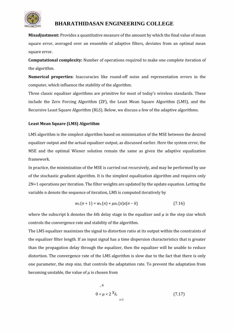
BHARATHIDASAN ENGINEERING COLLEGE
Misadjustment: Provides a quantitative measure of the amount by which the final value of mean
square error, averaged over an ensemble of adaptive filters, deviates from an optimal mean
square error.
Computational complexity: Number of operations required to make one complete iteration of
the algorithm.
Numerical properties: Inaccuracies like round-off noise and representation errors in the
computer, which influence the stability of the algorithm.
Three classic equalizer algorithms are primitive for most of today’s wireless standards. These
include the Zero Forcing Algorithm (ZF), the Least Mean Square Algorithm (LMS), and the
Recursive Least Square Algorithm (RLS). Below, we discuss a few of the adaptive algorithms.
Least Mean Square (LMS) Algorithm
LMS algorithm is the simplest algorithm based on minimization of the MSE between the desired
equalizer output and the actual equalizer output, as discussed earlier. Here the system error, the
MSE and the optimal Wiener solution remain the same as given the adaptive equalization
framework.
In practice, the minimization of the MSE is carried out recursively, and may be performed by use
of the stochastic gradient algorithm. It is the simplest equalization algorithm and requires only
2N+1 operations per iteration. The filter weights are updated by the update equation. Letting the
variable n denote the sequence of iteration, LMS is computed iteratively by
wk (n + 1) = wk (n) + µek (n)x(n − k) (7.16)
where the subscript k denotes the kth delay stage in the equalizer and µ is the step size which
controls the convergence rate and stability of the algorithm.
The LMS equalizer maximizes the signal to distortion ratio at its output within the constraints of
the equalizer filter length. If an input signal has a time dispersion characteristics that is greater
than the propagation delay through the equalizer, then the equalizer will be unable to reduce
distortion. The convergence rate of the LMS algorithm is slow due to the fact that there is only
one parameter, the step size, that controls the adaptation rate. To prevent the adaptation from
becoming unstable, the value of µ is chosen from
, N
0 < µ < 2 Xλi (7.17) i=1

BHARATHIDASAN ENGINEERING COLLEGE
where λi is the i-th eigenvalue of the covariance matrix R.
Normalized LMS (NLMS) Algorithm
In the LMS algorithm, the correction that is applied to wk (n) is proportional to the input sample
x(n − k). Therefore when x(n − k) is large, the LMS algorithm experiences gradient noise
amplification. With the normalization of the LMS step size by kx(n)k2 in the NLMS algorithm, this
problem is eliminated. Only when x(n−k) becomes close to zero, the denominator term kx(n)k2 in
the NLMS equation becomes very small and the correction factor may diverge. So, a small positive
number ε is added to the denominator term of the correction factor. Here, the step size is time
varying and is expressed as
. (7.18)
Therefore, the NLMS algorithm update equation takes the form of
. (7.19)
7.3 Diversity
Diversity is a method used to develop information from several signals transmitted over
independent fading paths. It exploits the random nature of radio propagation by finding
independent signal paths for communication. It is a very simple concept where if one path
undergoes a deep fade, another independent path may have a strong signal. As there is more than
one path to select from, both the instantaneous and average SNRs at the receiver may be
improved. Usually diversity decisions are made by receiver. Unlike equalization, diversity
requires no training overhead as a training sequence is not required by transmitter. Note that if
the distance between two receivers is a multiple of λ/2, there might occur a destructive
interference between the two signals. Hence receivers in diversity technique are used in such a
way that the signal received by one is independent of the other. Diversity can be of various forms,
starting from space diversity to time diversity. We take up the types one by one in the sequel.

BHARATHIDASAN ENGINEERING COLLEGE
Figure 7.3: Receiver selection diversity, with M receivers.
7.3.1 Different Types of Diversity
Space Diversity
A method of transmission or reception, or both, in which the effects of fading are minimized by
the simultaneous use of two or more physically separated antennas, ideally separated by one half
or more wavelengths. Signals received from spatially separated antennas have uncorrelated
envelopes.
Space diversity reception methods can be classified into four categories: selection, feedback or
scanning, maximal ratio combining and equal gain combining.
(a) Selection Diversity:
The basic principle of this type of diversity is selecting the best signal among all the signals
received from different branches at the receiving end. Selection Diversity is the simplest diversity
technique. Figure 7.3 shows a block diagram of this method where ’M’ demodulators are used to
provide M diversity branches whose gains are adjusted to provide the same average SNR for each
branch. The receiver branches having the highest instantaneous SNR is connected to the
demodulator.
Let M independent Rayleigh fading channels are available at a receiver. Each channel is called a
diversity branch and let each branch has the same average SNR. The signal to noise ratio is
defined as
(7.20)

BHARATHIDASAN ENGINEERING COLLEGE
where Eb is the average carrier energy, N0 is the noise PSD, α is a random variable used to
represent amplitude values of the fading channel.
The instantaneous SNR(γi) is usually defined as γi = instantaneous signal power per branch/mean
noise power per branch. For Rayleigh fading channels, α has a Rayleigh distribution and so α2 and
consequently γi have a chi-square distribution with two degrees of freedom. The probability
density function for such a channel is
. (7.21)
The probability that any single branch has an instantaneous SNR less than some defined
threshold γ is
γ γ
Pr[ . (7.22) 0 0
Similarly, the probability that all M independent diversity branches receive signals which are
simultaneously less than some specific SNR threshold γ is
Pr[ ) (7.23)
where PM (γ) is the probability of all branches failing to achieve an instantaneous SNR = γ. Quite
clearly, PM(Γ) < P(Γ). If a single branch achieves SNR > γ, then the probability that SNR > γ for one
or more branches is given by
M Pr[ (7.24)
which is more than the required SNR for a single branch receiver. This expression shows the
advantage when a selection diversity is used.
To determine of average signal to noise ratio, we first find out the pdf of γ as
. (7.25)
The average SNR, ¯γ, can be then expressed as
(7.26)
where x = γ/Γ and Γ is the average SNR for a single branch, when no diversity is
used.

BHARATHIDASAN ENGINEERING COLLEGE
This equation shows an average improvement in the link margin without requiring extra
transmitter power or complex circuitry, and it is easy to implement as it needed a monitoring
station and an antenna switch at the receiver. It is not an optimal diversity technique as it doesn’t
use all the possible branches simultaneously. (b) Feedback or Scanning Diversity:
Scanning all the signals in a fixed sequence until the one with SNR more than a predetermined
threshold is identified. Feedback or scanning diversity is very similar to selection diversity except
that instead of always using the best of N signals, the N signals are scanned in a fixed sequence
until one is found to be above a predetermined threshold. This signal is then received until it falls
below threshold and the scanning process is again initiated. The resulting fading statistics are
somewhat inferior, but the advantage is that it is very simple to implement(only one receiver is
required). (c) Maximal Ratio Combining:
Signals from all of the m branches are weighted according to their individual signal voltage to
noise power ratios and then summed. Individual signals must be cophased before being summed,
which generally requires an individual receiver and phasing circuit for each antenna element.
Produces an output SNR equal to the sum of all individual SNR. Advantage of producing an output
with an acceptable
SNR even when none of the individual signals are themselves acceptable. Modern DSP techniques
and digital receivers are now making this optimal form, as it gives the best statistical reduction
of fading of any known linear diversity combiner. In terms of voltage signal,
m
rm = XGiri (7.27) i=1
where Gi is the gain and ri is the voltage signal from each branch.
(d) Equal Gain Combining:
In some cases it is not convenient to provide for the variable weighting capability required for
true maximal ratio combining. In such cases, the branch weights are all set unity, but the signals
from each branch are co-phased to provide equal gain combining diversity. It allows the receiver
to exploit signals that are simultaneously received on each branch. Performance of this method
is marginally inferior to maximal ratio combining and superior to Selection diversity. Assuming
all the Gi to be

BHARATHIDASAN ENGINEERING COLLEGE
Figure 7.4: Maximal ratio combining technique.
unity, here,
. (7.28)
Polarization Diversity
Polarization Diversity relies on the decorrelation of the two receive ports to achieve diversity
gain. The two receiver ports must remain cross-polarized. Polarization Diversity at a base station
does not require antenna spacing. Polarization diversity combines pairs of antennas with
orthogonal polarizations (i.e. horizontal/vertical, ± slant 45o, Left-hand/Right-hand CP etc).
Reflected signals can undergo polarization changes depending on the channel. Pairing two
complementary polarizations, this scheme can immunize a system from polarization mismatches
that would otherwise cause signal fade. Polarization diversity has prove valuable at radio and
mobile communication base stations since it is less susceptible to the near random orientations
of transmitting antennas.
BHARATHIDASAN ENGINEERING COLLEGE
Frequency Diversity
In Frequency Diversity, the same information signal is transmitted and received simultaneously
on two or more independent fading carrier frequencies. Rationale behind this technique is that
frequencies separated by more than the coherence bandwidth of the channel will be uncorrelated
and will thus not experience the same fades. The probability of simultaneous fading will be the
product of the individual fading probabilities. This method is employed in microwave LoS links
which carry several channels in a frequency division multiplex mode (FDM). Main disadvantage
is that it requires spare bandwidth also as many receivers as there are channels used for the
frequency diversity.
Time Diversity
In time diversity, the signal representing the same information are sent over the same channel at
different times. Time diversity repeatedly transmits information at time spacings that exceeds
the coherence time of the channel. Multiple repetition of the signal will be received with
independent fading conditions, thereby providing for diversity. A modern implementation of time
diversity involves the use of RAKE receiver for spread spectrum CDMA, where the multipath
channel provides redundancy in the transmitted message. Disadvantage is that it requires spare
bandwidth also as many receivers as there are channels used for the frequency diversity. Two
important types of time diversity application is discussed below.
Application 1: RAKE Receiver
In CDMA spread spectrum systems, CDMA spreading codes are designed to provide very low
correlation between successive chips, propagation delay spread in the radio channel provides
multiple version of the transmitted signal at the receiver. Delaying multipath components by
more than a chip duration, will appear like uncorrelated noise at a CDMA receiver. CDMA receiver
may combine the time delayed versions of the original signal to improve the signal to noise ratio
at the receiver. RAKE

BHARATHIDASAN ENGINEERING COLLEGE
Figure 7.5: RAKE receiver.
receiver collect the time shifted versions of the original signal by providing a separate correlation
receiver for M strongest multipath components. Outputs of each correlator are weighted to
provide a better estimate of the transmitted signal than provided by a single component.
Demodulation and bit decisions are based on the weighted output of the correlators. Schematic
of a RAKE receiver is shown in Figure
7.5.
Application 2: Interleaver
In the encoded data bits, some source bits are more important than others, and must be protected
from errors. Many speech coder produce several important bits in succession. Interleaver spread
these bit out in time so that if there is a deep fade or noise burst, the important bits from a block
of source data are not corrupted at the same time. Spreading source bits over time, it becomes
possible to make use of error control coding. Interleaver can be of two forms, a block structure
or a convolutional structure.
A block interleaver formats the encoded data into a rectangular array of m rows and n columns,
and interleaves nm bits at a time. Each row contains a word of source data having n bits. an
interleaver of degree m consists of m rows. source bits are placed into the interleaver by
sequentially increasing the row number for each successive bit, and forming the columns. The
interleaved source data is then read out row-wise and transmitted over the channel. This has the

BHARATHIDASAN ENGINEERING COLLEGE
effect of separating the original source bits by m bit periods. At the receiver, de-interleaver stores
the received data by sequentially increasing the row number of each successive bit, and then
clocks out the data row-wise, one word at a time. Convolutional interleavers are ideally suited for
use with convolutional codes.

BHARATHIDASAN ENGINEERING COLLEGE
UNIT V MULTIPLE ANTENNA TECHNIQUES
MIMO systems – spatial multiplexing -System model -Pre-coding - Beam forming -
transmitter diversity, receiver diversity- Channel state information-capacity in fading
and non-fading channels
• When multiple antennas are available at the receiver, the transmission quality can be improved
through exploiting receive beamforming. This method is useful for uplink (from mobile terminal to
base station) as the base station can usually be equipped with multiple antennas. • Equipping
multiple antennas at the mobile terminal side may not be practical due to size limitation and
complexity constraint. Thus it is difficult to improve the performance of downlink (from base station
to mobile terminal) using receive beamforming.
• In this case, we may consider using the base station antennas to improve the downlink performance.
– Transmit beamforming: When the channel state information at the transmitter (CSIT) is
known, transmit beamforming can be used
to achieve diversity gain as well as array gain.
– Transmit diversity: When CSIT is not available, transmit diversity technique can be used to
achieve diversity gain.
• If mobile terminal is also equipped with multiple antennas, transmit beamforming/diversity can be
jointly deployed with receive beamforming to further improve the uplink and downlink performance.
• Outline of this lecture:
– System model: MISO channel
– Transmit beamforming with CSIT
– Transmit diversity without CSIT: Alamouti code
– Joint transmit and receive beamforming for MIMO channel with both CSIT and CSIR
– Joint transmit diversity and receive beamforming for MIMO channel with CSIR only

BHARATHIDASAN ENGINEERING COLLEGE
Consider the following MISO channel:
y(n) = hT x(n) + z(n) (1)
– x(n) = [x1(n),...,xt(n)]T ; t denotes the number of transmit antennas
– h = [h1,...,ht]T ; hi = √βiejθi,i = 1,...,t, where βi = |hi|2 and θi = ∠hi
– Assume a sum-power constraint at the transmitter (for the time being): E[kx(n)k2] ≤ P, where P
denotes the sum-power constraint over all transmit antennas
–
Transmit Beamforming with
CSIT
• Transmitted signal: x(n) = ws(n)

BHARATHIDASAN ENGINEERING COLLEGE
– Transmit beamforming vector: w = [w1,...,wt]T ∈ Ct×1
– Information signal: s(n) ∈ C
• Sum-power constraint
– E[|s(n)|2] = 1
– kwk2 ≤ P
– E[kx(n)k2] = kwk2E[|s(n)|2] ≤ P × 1 = P
• Received signal is
Xi=1
• The instantaneous receiver SNR is
defined as
(4)
(5)
• It is desirable to choose w to maximize γ subject to kwk2 ≤ P.
y(n) = hT ws(n) + z(n) (2)
=
t
hiwi!s(n) + z(n) (3)

BHARATHIDASAN ENGINEERING COLLEGE
• It is also desirable to require only partial knowledge of h at the transmitter to design w, because in
practice the CSI is usually difficult to obtain at the transmitter side. • There are two commonly
adopted methods to obtain CSIT for a link that has two-way communications:
– If the link employs a time-division-duplex (TDD) method to switch transmissions between two
nodes over the same frequency band, the channel from one node to the other can be highly
correlated with that in the reverse transmit direction, a phenomenon so-called channel
reciprocity. Thus, one node can obtain the channel to the other by estimating the reverse
channel from the other node to itself.
– If the link employs a frequency-division-duplex (FDD) method to allow both nodes to transmit
at the same time slot but over different frequency bands, the channel over which one node
transmits to the other can be different from that over which it receives from the other. Thus,
the channel reciprocity may not hold and the first method to obtain CSIT may fail. However,
one node can help the other node obtain CSIT by estimating the channel from the other node
and then sending it back to the other node, a technique so-called CSI feedback. • Three
transmit beamforming schemes are considered:
– Antenna selection (AS)
– Pre-equal-gain-combining (P-EGC)
– Pre-maximal-ratio-combining (P-MRC)
• For AS, only the antenna with the largest instantaneous channel gain is
index of the transmit antenna that has the largestselected for transmission at each time. Let j ∈ 1,...,tβj
=|hdenote thej|2. Then, the
transmit beamforming weights for AS are
AS = √P if i = j i = 1,...,t (6) w
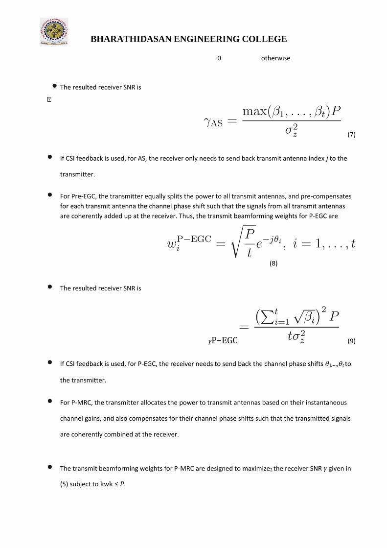
BHARATHIDASAN ENGINEERING COLLEGE
0 otherwise
• The resulted receiver SNR is
(7)
• If CSI feedback is used, for AS, the receiver only needs to send back transmit antenna index j to the
transmitter.
• For Pre-EGC, the transmitter equally splits the power to all transmit antennas, and pre-compensates
for each transmit antenna the channel phase shift such that the signals from all transmit antennas
are coherently added up at the receiver. Thus, the transmit beamforming weights for P-EGC are
(8)
• The resulted receiver SNR is
γP−EGC (9)
• If CSI feedback is used, for P-EGC, the receiver needs to send back the channel phase shifts θ1,...,θt to
the transmitter.
• For P-MRC, the transmitter allocates the power to transmit antennas based on their instantaneous
channel gains, and also compensates for their channel phase shifts such that the transmitted signals
are coherently combined at the receiver.
• The transmit beamforming weights for P-MRC are designed to maximize2 the receiver SNR γ given in
(5) subject to kwk ≤ P.

BHARATHIDASAN ENGINEERING COLLEGE
• First, we have the following inequalities:
(10)
where the first inequality is due to Cauchy-Schwarz
inequality, and holds with equality iff , with c being any
complex number, while the second inequality holds with
. equality when
• To make the above two equalities hold at the same time, we have
, yielding
(11) • Thus we obtain the transmit beamforming weights for P-
MRC as
(12)
• The maximum receiver SNR achieved by the P-MRC transmit beamforming is
γP−MRC (13)
• If CSI feedback is applied, for P-MRC, the receiver needs to send back the instantaneous channels
h1,...,ht to the transmitter.

BHARATHIDASAN ENGINEERING COLLEGE
• The outage probability, diversity order, and array gain analysis for the MISO channel with AS, P-EGC,
and P-MRC transmit beamforming is similar to that for the SIMO channel with SC, EGC, and MRC
receive beamforming given in Lecture II, respectively. Thus we omit the details here (while it is still
worthwhile verifying them by yourself !!!).
• Example: Consider an iid Rayleigh fading MISO channel with h ∼ hw.
If t = 1 (i.e., a SISO system), the instantaneous receiver SNR is
. Using (13) and the results we have derived for the MRC
receive beamforming in the SIMO channel case, it can be easily shown that the diversity order and
array gain for P-MRC transmit beamforming are both equal to t.
Per-Antenna Power Constraint
• So far, we have studied transmit beamforming for the MISO channel subject to the sum-power
constraint at the transmitter. In practice, the per-antenna-based transmit power constraint is usually
more relevant than the sum-power constraint, due to the fact that each transmit antenna has its
own power amplifier which operates properly only when the transmit power is below a predesigned
threshold.
• Under the per-antenna power constraint, the transmit beamforming weights need to satisfy
|wi|2 ≤ P0,i = 1,...,t (14)
where P0 denotes the transmit power constraint for each antenna. • What are the
optimal transmit beamforming weights in this case?
Answer: P-EGC with transmit power P0 at all antennas (Why?)
Transmit Diversity Without CSIT
• Consider the simplest case of t = 2.
• In the case without CSIT, how to achieve the MISO channel (with iid h1 and h2) diversity gain over a
SISO channel (with only h1 or h2)?

BHARATHIDASAN ENGINEERING COLLEGE
• Two heuristic schemes:
– Power Splitting
x
(15)
– Alternate Transmission
x
x
(16)
• For power splitting, the received signal can be written as
)
(17)
• Assuming that h1 and h2 are iid CSCG RVs with zero mean and variance σh2, thus (h1 + h2)/√2 is also a
CSCG RV with zero mean and the same variance. Thus the received signal is statistically equivalent to
that over the following SISO channel
y(n) = h1√Ps(n) + z(n) (18)
• Therefore, power splitting does not provide any diversity gain over the SISO system.
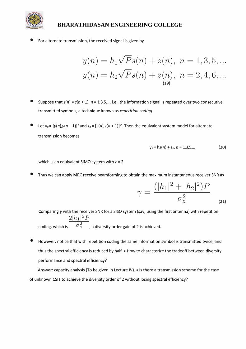
BHARATHIDASAN ENGINEERING COLLEGE
• For alternate transmission, the received signal is given by
(19)
• Suppose that s(n) = s(n + 1), n = 1,3,5,..., i.e., the information signal is repeated over two consecutive
transmitted symbols, a technique known as repetition coding.
• Let yn = [y(n),y(n + 1)]T and zn = [z(n),z(n + 1)]T . Then the equivalent system model for alternate
transmission becomes
yn = hs(n) + zn, n = 1,3,5,... (20)
which is an equivalent SIMO system with r = 2.
• Thus we can apply MRC receive beamforming to obtain the maximum instantaneous receiver SNR as
(21)
Comparing γ with the receiver SNR for a SISO system (say, using the first antenna) with repetition
coding, which is , a diversity order gain of 2 is achieved.
• However, notice that with repetition coding the same information symbol is transmitted twice, and
thus the spectral efficiency is reduced by half. • How to characterize the tradeoff between diversity
performance and spectral efficiency?
Answer: capacity analysis (To be given in Lecture IV). • Is there a transmission scheme for the case
of unknown CSIT to achieve the diversity order of 2 without losing spectral efficiency?

BHARATHIDASAN ENGINEERING COLLEGE
Alamouti Code
• Transmitted signals at symbol time n = 1,2 are
x
(22)
• Similar for n = 3,4, n = 5,6,...
• Received signals are
(2)
(23)
• Let y = [y(1),y∗(2)]T , s = [s(1),s(2)]T , and z = [z(1),z∗(2)]T . The equivalent 2 × 2 MIMO channel becomes
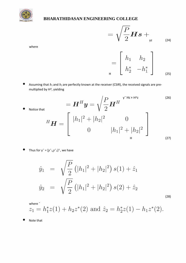
BHARATHIDASAN ENGINEERING COLLEGE
yz (24)
where
H (25)
• Assuming that h1 and h2 are perfectly known at the receiver (CSIR), the received signals are pre-
multiplied by HH, yielding
yˆ Hs + HHz (26)
• Notice that
H (27)
• Thus for yˆ = [yˆ1,yˆ2]T , we have
(28)
where ˆ
• Note that
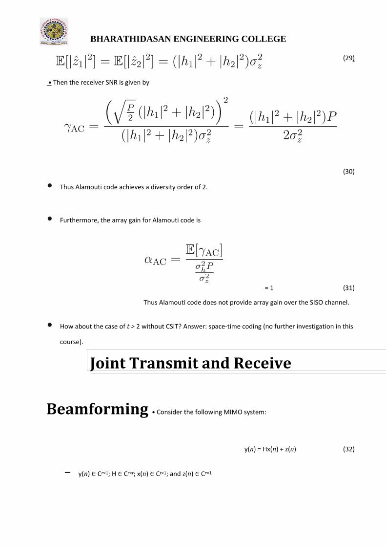
BHARATHIDASAN ENGINEERING COLLEGE
(29)
• Then the receiver SNR is given by
(30)
• Thus Alamouti code achieves a diversity order of 2.
• Furthermore, the array gain for Alamouti code is
= 1 (31)
Thus Alamouti code does not provide array gain over the SISO channel.
• How about the case of t > 2 without CSIT? Answer: space-time coding (no further investigation in this
course).
Joint Transmit and Receive
Beamforming • Consider the following MIMO system:
y(n) = Hx(n) + z(n) (32)
– y(n) ∈ Cr×1; H ∈ Cr×t; x(n) ∈ Ct×1; and z(n) ∈ Cr×1

BHARATHIDASAN ENGINEERING COLLEGE
– z
– x(n) = wts(n), where wt ∈ Ct×1 denotes the transmit beamforming vector, which satisfies the
sum-power constraint: kwtk2 ≤ P
– Assume both known CSIT and CSIR
• The receive beamforming vector is denoted by wr ∈ Cr×1. After applying wr to the received signal
vector, the resultant receiver output is (the symbol index n is dropped by brevity)
Hw
z (33)
• The receiver output SNR is then defined as
2
γ
| (34)
• It is desirable to jointly choose wt and wr to maximize γ subject to kwtk2 ≤ P.
• Possible schemes:
– AS at Tx and SC at Rx
– AS at Tx and MRC at Rx – P-MRC at Tx and SC at Rx
– ...
• Next, we find the optimal wt and wr to maximize γ.
• According to Cauchy-Schwarz inequality, we have for any given wt
= [ | H
r
t s | 2 ]
[ | H r
| 2 ] =
| H r
t
| 2 [ | s | 2 ]
H r
[ H ] r
= | H
r
t k
r k 2 σ 2
z

BHARATHIDASAN ENGINEERING COLLEGE
(35)
where equality holds iff wr = cHwt, with c being any complex number. For convenience, we set c to
make kwrk = 1, thus c = 1/kHwtk.
• The above SNR upper bound is maximized when wt maximizes kHwtk2 subject to kwtk2 ≤ P.
• Let the singular-value decomposition (SVD) of H be denoted by
H = UΛV H (36)
where U ∈ Cr×r with UUH = UHU = Ir; V ∈ Ct×t with
VV H = V HV = It; and Λ is a r × t matrix, the elements of which are all zeros, except that [Λ]i,i = λi > 0,
i = 1,...,m with m = Rank(H) ≤ min(t,r). It is assumed that λ1 ≥ ... ≥ λm > 0.
• Then the maximization of kHwtk2 becomes equivalent to
w Hw
(37)
• Let w˜ t = V Hwt and thus wt = Vw˜ t. The power constraint for w˜ t becomes
VV Hwt = kwtk2 ≤ P.
• The maximization problem then becomes equivalent to
Maximize kΛw˜ tk2 subject to : kw˜ tk2 ≤ P (38)
• It is easy to verify that the optimal solution for w˜ t is

BHARATHIDASAN ENGINEERING COLLEGE
w˜ topt , and the maximum objective value
is .
• Let V = [v1,...,vt] and U = [u1,...,ur].
• Then it follows that the optimal transmit beamforming vector is
woptt = Vw˜ optt = √
Pv1 (39)
and the optimal receive beamforming vector is
Hwopt λ √P u
woptr k √ u1 (40) Hwt k
λ1 P
• From (35), the resultant maximum receiver SNR is
γopt (41)
• Substituting woptt and woptr into (33) yields
where ˆ
Thus, the MIMO channel is converted to an equivalent SISO channel by joint transmit and receive
beamforming, which is usually called “strongest eigenmode beamforming (SEB)”.
• Sanity check: what is the optimal transmit/receive beamforming vector when t = 1 or r = 1?
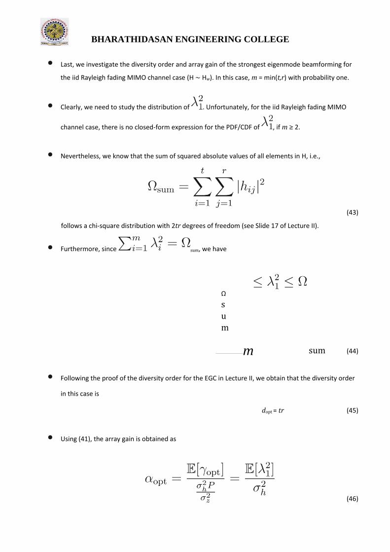
BHARATHIDASAN ENGINEERING COLLEGE
• Last, we investigate the diversity order and array gain of the strongest eigenmode beamforming for
the iid Rayleigh fading MIMO channel case (H ∼ Hw). In this case, m = min(t,r) with probability one.
• Clearly, we need to study the distribution of . Unfortunately, for the iid Rayleigh fading MIMO
channel case, there is no closed-form expression for the PDF/CDF of , if m ≥ 2.
• Nevertheless, we know that the sum of squared absolute values of all elements in H, i.e.,
(43)
follows a chi-square distribution with 2tr degrees of freedom (see Slide 17 of Lecture II).
• Furthermore, since sum, we have
Ω
s
u
m
m sum (44)
• Following the proof of the diversity order for the EGC in Lecture II, we obtain that the diversity order
in this case is
dopt = tr (45)
• Using (41), the array gain is obtained as
(46)

BHARATHIDASAN ENGINEERING COLLEGE
• Using the fact that E[Ωsum] = trσh2 and (44), it follows that
(47)
The upper and lower bounds become equal when t = 1 or r = 1.
Joint Transmit Diversity and Receive
Beamforming
• Consider the following r × 2 MIMO system:
y(n) = Hx(n) + z(n) (48)
– H ∈ Cr×2 = [h1,...,hr]T , where hi ∈ C2×1,i = 1,...,r
– y(n) ∈ Cr×1; x(n) ∈ C2×1; and z(n) ∈ Cr×1
– z
– E[kx(n)k2] ≤ P
– Assume known CSIR only (unknown CSIT)
• Transmitter scheme: Alamouti code (AC)
• Receiver scheme: independently decodes the AC at each receive antenna and then applies MRC to
combine the decoded output signals from all receive antennas
tr
m
≤ α opt
≤ tr ⇒ max( t,r ) ≤ α opt
≤ tr
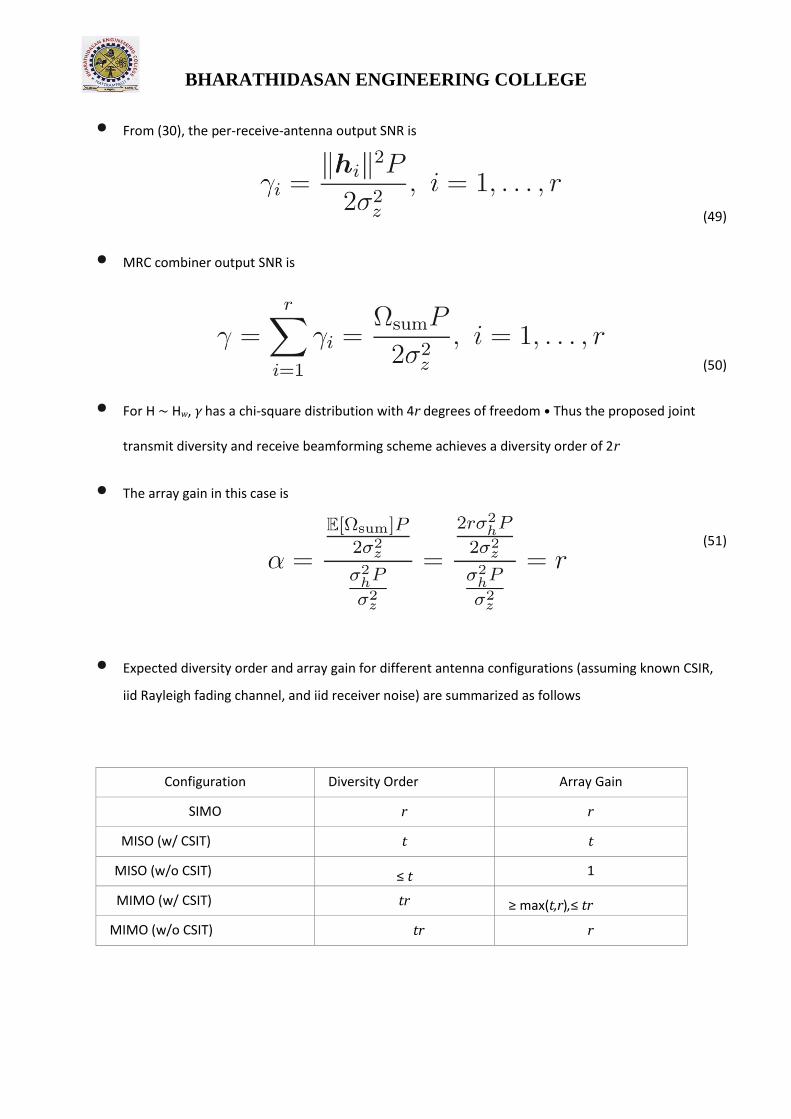
BHARATHIDASAN ENGINEERING COLLEGE
• From (30), the per-receive-antenna output SNR is
(49)
• MRC combiner output SNR is
(50)
• For H ∼ Hw, γ has a chi-square distribution with 4r degrees of freedom • Thus the proposed joint
transmit diversity and receive beamforming scheme achieves a diversity order of 2r
• The array gain in this case is
(51)
• Expected diversity order and array gain for different antenna configurations (assuming known CSIR,
iid Rayleigh fading channel, and iid receiver noise) are summarized as follows
Configuration Diversity Order Array Gain
SIMO r r
MISO (w/ CSIT) t t
MISO (w/o CSIT) ≤ t 1
MIMO (w/ CSIT) tr ≥ max(t,r),≤ tr
MIMO (w/o CSIT) tr r