11 capacity

8/13/2019 11 Capacity

http://slidepdf.com/reader/full/11-capacity 1/71

Wireless Network Capacity

Jamar Parris

Xi Liu

8/13/2019 11 Capacity


Areas Covered

Fixed Nodes

Mobility of Nodes

8/13/2019 11 Capacity


Focus

All wireless networks

Causes issues:

Medium access issues

No centralized control complicates matters

Physical layer issues

Transmission power must be high enough to reach

receiver whilst causing minimal interference to others.

Fixed Nodes Mobility of Nodes

8/13/2019 11 Capacity


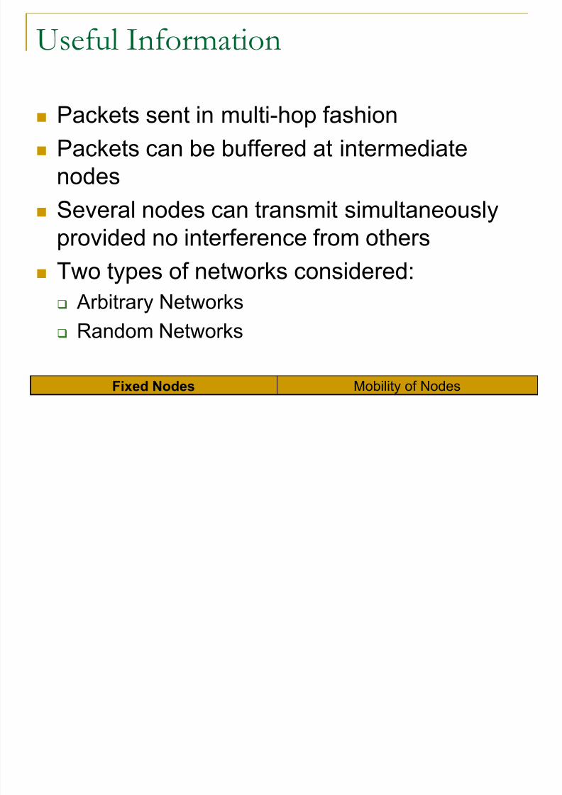
Useful Information

Packets sent in multi-hop fashion

Packets can be buffered at intermediate

nodes

Several nodes can transmit simultaneously

provided no interference from others

Two types of networks considered:

Arbitrary Networks

Random Networks


8/13/2019 11 Capacity


Arbitrary Networks

Node locations, destinations, traffic demands,

range are all arbitrary.

2 models used to describe successful

transmission from hop to hop:

Protocol Model

Physical Model

Adds a signal to interference ratio Adds a ambient power level


8/13/2019 11 Capacity


Arbitrary Networks

Assume 1 bit meter is when one bit is

transported the distance of 1 meter

Multiple credit not given for same bit carried

to several destinations e.g. multicast

Sum of products of bits and distances over

which they are carried indicates transport

capacity


8/13/2019 11 Capacity


Arbitrary Networks – Results

Transport capacity under Protocol Model is

This depends on:

Nodes being optimally placed

Traffic pattern optimally chosen

Transmission range being optimally chosen.


8/13/2019 11 Capacity


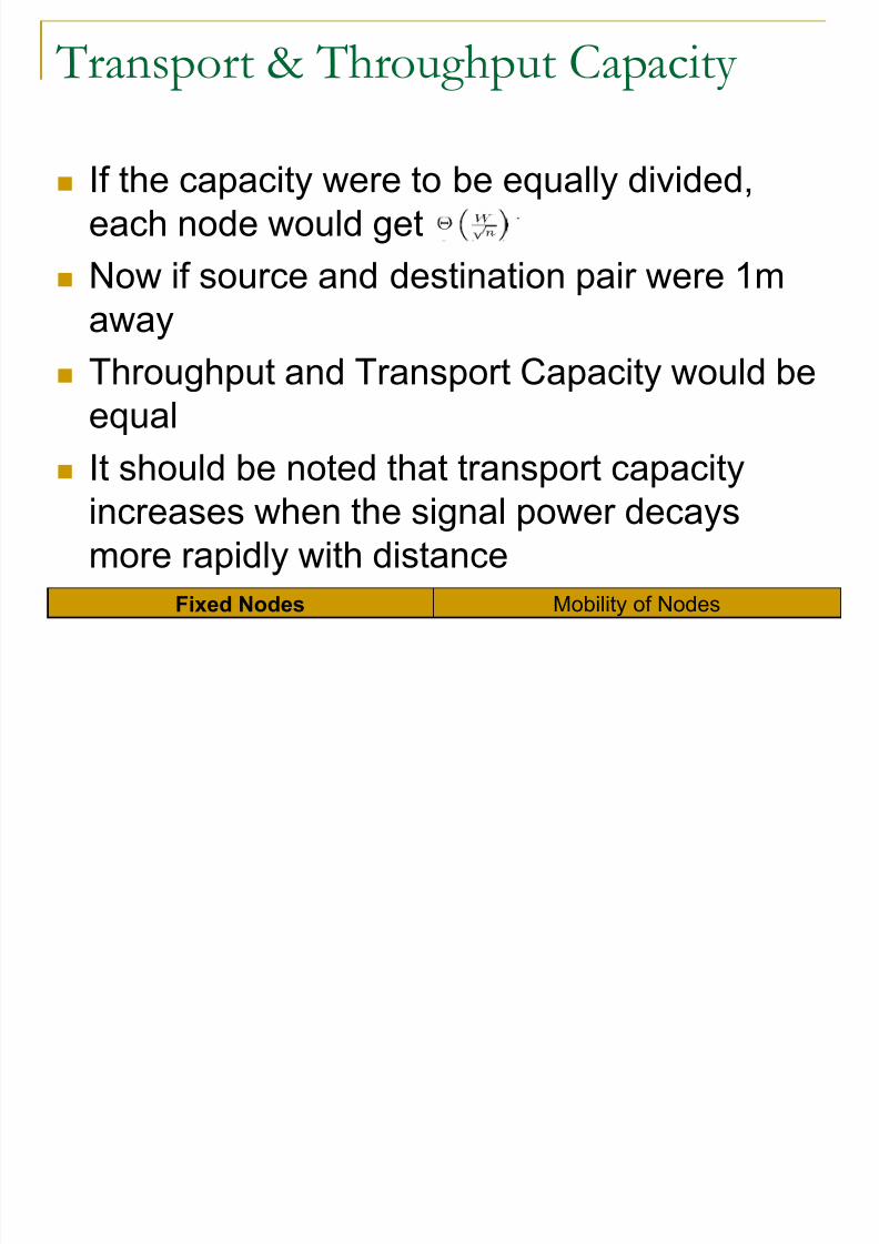
Transport & Throughput Capacity

If the capacity were to be equally divided,

each node would get

Now if source and destination pair were 1m

away

Throughput and Transport Capacity would be

equal

It should be noted that transport capacityincreases when the signal power decays

more rapidly with distance


8/13/2019 11 Capacity


Random Networks

Each node randomly chooses destination

Destination chosen independently as the

node closest to a randomly located point

All transmissions use the same range

Nodes are randomly located either on the

surface of a sphere or in a plane


8/13/2019 11 Capacity


Random Networks

Sphere:

Every node in a cell is within range of every other

node in its own cell or adjacent cells

If two cells are not interfering neighbors than theirtransmissions cannot collide.

Number of interfering neighbors are bounded so

that each cell has chance to transmit.

Each cell contains at least one node to make

relaying feasible.


8/13/2019 11 Capacity


Sphere


8/13/2019 11 Capacity


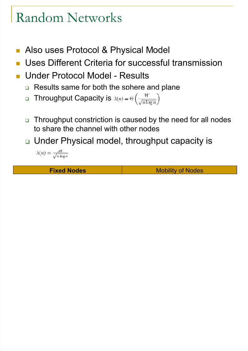
Random Networks

Also uses Protocol & Physical Model

Uses Different Criteria for successful transmission

Under Protocol Model - Results

Results same for both the sphere and plane Throughput Capacity is

Throughput constriction is caused by the need for all nodes

to share the channel with other nodes Under Physical model, throughput capacity is


8/13/2019 11 Capacity


Relay Nodes

Idea is to add additional nodes who only relay

packets and are not themselves sources

This allows for an increase in throughput

However, number of relay nodes to have an

significant increase in capacity can be large.

For example, with 100 nodes, to make

capacity equal to five times its value whenthere are no relay nodes, you need 4476

relays.


8/13/2019 11 Capacity


Trade-Offs

Throughput versus range

Increasing range of each node would reduce hops

traversed. However, since nodes close to receiver

need to be idle to avoid collision, throughputwould actually decrease.

Actually reducing range to as small as possible is

what’s needed.

However, range can only get so small before thenetwork loses connectivity


8/13/2019 11 Capacity


Inferences of the paper

Maybe you should group nodes into cells and

then designate one node to carry the burden

of relaying multi-hop packets.

Maybe connect base stations by wired linksto improve capacity.

If we assign a base station in each cell to

communicate with other distant base stationswirelessly, base stations inherit same

capacity limitation.


8/13/2019 11 Capacity


Inferences of Paper

According to tests, subdividing the channel W

into W1, W2, etc. did not change anything.

As number of nodes increase throughput will

also decrease.


8/13/2019 11 Capacity


Issues with this paper

Interference is not factored in

Access to wireless channel not coordinated

Mobility not included

Link failures not included Hence adapted and distributed traffic routing not

included.

Claims that the above will only reducecapacity. Not all of these is necessarily true


8/13/2019 11 Capacity


Mobility of Nodes

Follows the same model, only nodes are

mobile as opposed to fixed

Network Topology changes over time

Incurs delay, good for applications that can

tolerate delays of minutes to even hours.

E-Mail

Database Synchronization


8/13/2019 11 Capacity


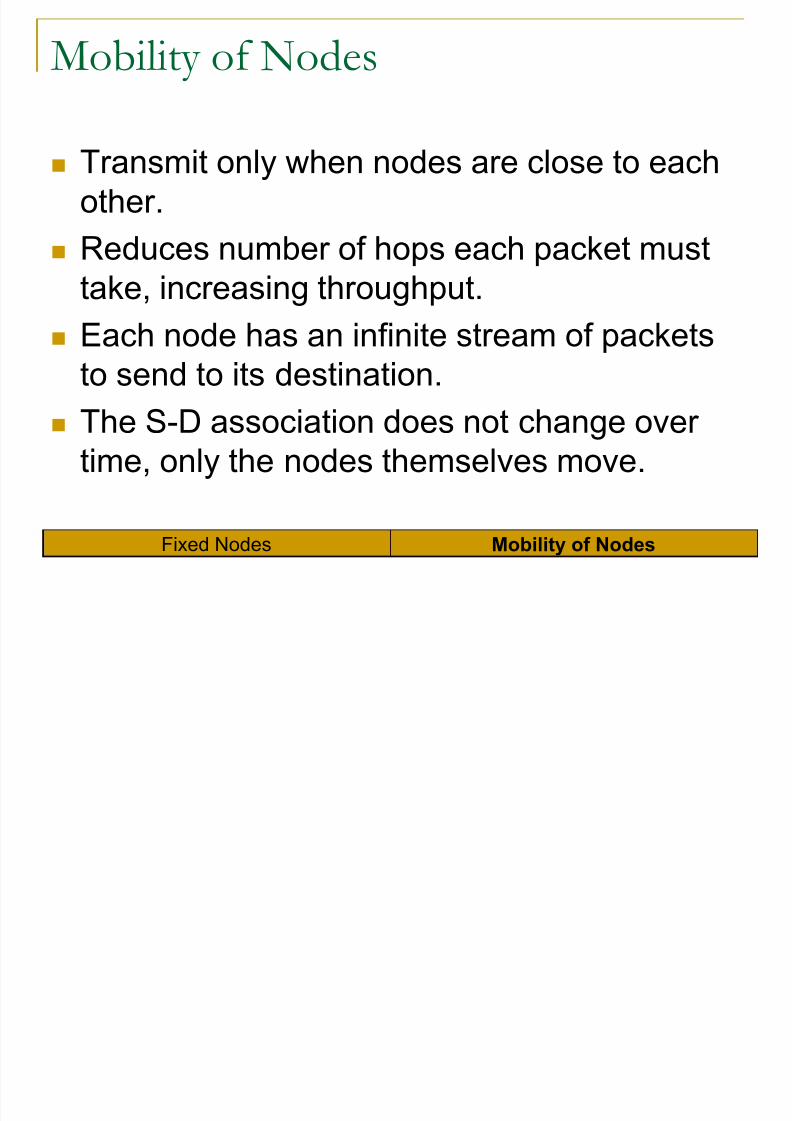
Mobility of Nodes

Transmit only when nodes are close to each

other.

Reduces number of hops each packet must

take, increasing throughput.

Each node has an infinite stream of packets

to send to its destination.

The S-D association does not change overtime, only the nodes themselves move.


8/13/2019 11 Capacity


Two Scenarios Used

Mobile Nodes without Relaying

Mobile Nodes with Relaying

Fixed NodesMobility of Nodes

8/13/2019 11 Capacity


Mobile Nodes without Relaying

The problem with fixed nodes is thatthroughput reaches zero because number ofrelay nodes packet must go through

increases In this scenario, we expect that any two

nodes can be expected to be close to eachother from time to time.

Improve capacity by not relaying at all andonly let sources transmit directly todestinations.


8/13/2019 11 Capacity


Results

If the range is large (i.e. transmissions over longdistances are allowed). many S-D pairs are withinrange.

Interference however will limit the number of

concurrent transmissions over long distances Makes throughput interference limited

Also, if range is small, only a small fraction of S-Dpairs will be close enough to transmit a packet.

Makes throughput distance limited.

Throughput per session decreases as n gets largerif only direct transmissions are allowed.


8/13/2019 11 Capacity


Mobile Nodes With Relaying

Problems with no relaying: Find a way to communicate only locally to

overcome interference limitation

Find a way to ensure that there are enoughsender-receiver pairs to transmit to overcomedistance limitation

Proposed Solution: Direct communication not enough, so introduce

relaying.


8/13/2019 11 Capacity


Basic Idea

Spread the traffic stream between the sourceand destination to a large number ofintermediate relay nodes

Each packet goes through one relay thatbuffers the packet until final destinationdelivery is possible

For each S-D, every other node except S & D

can serve as relay nodes Goal is packets of every source node will be

distributed across all nodes in the network


8/13/2019 11 Capacity


Basic Idea

This ensures that every other node in the

network will have packets buffered destined

to every other node not including itself

Hence, a sender-receiver pair always has apacket to send unlike in the case without

relaying

How many times must a packet be relayed inorder to spread traffic uniformly?


8/13/2019 11 Capacity


Number of Hops per packet

It turns out only one

The probability of an arbitrary node to bescheduled to receive a packet from source S

in equal for all nodes and independent of S Each packet therefore has to make only two

hops Source to relay

Relay to destination

Total achievable throughput is


8/13/2019 11 Capacity


2 Phases

Phase 1 Scheduling of packet transmissions from source to relays

or from source to final destination in one hop if possible

Phase 2 Scheduling of transmissions from relay to final destination

or from source to destination if possible.

When a receiver is identified, sender checks to see if it hasany packets for which receiver is the destination, if it is, ittransmits.

In either phase, direct transmission is allowed since it ispossible for a sender receiver pair to be a sourcedestination pair as well.


8/13/2019 11 Capacity


Phase 1 & Phase 2


8/13/2019 11 Capacity


Centralized vs. Distributed

Implementation

This model allowed for central coordinatedscheduling, relaying and routing.

Authors believe algorithm can be

implemented in a distributed manner as well In this case:

At each instant, node can randomly andindependently determine if they want to be a

sender or potential receiver Each sender seeks out a receiver close to it and

attempts to send data to it


8/13/2019 11 Capacity


Distributed Implementation

Same phases as in centralized

Multiple senders may attempt to send to

same receiver

Author’s analysis showed that probability of

success is reasonable even with many users


8/13/2019 11 Capacity


Problem

Since capacity in both phases are identical,

delay experienced from source to destination

can be infinite even for a finite number of

nodes if capacity in phase 1 fully used. Author Fix?

Allow both source to relay and relay to destination

transmissions to occur concurrently but givepriority to relay to destination transmissions.


8/13/2019 11 Capacity


Sender Centric versus Receiver Centric

So far, sender selects the closest receiver to

send to

What if receiver selects the closest sender

from which to receive?

At first, it may seem that results should be

the same, but in fact this is not the case

Problems occur if several receivers select thesame sender


8/13/2019 11 Capacity


Two possible outcomes

If the sender can only select one receiver to

send to, sender-receiver pairs need to be

eliminated,

If sender can generate multiple signals forseveral receivers, we need to account for the

fact the desired signal is only a fraction of unit

power. Authors found no elegant want to integrate

these complications into the proof


8/13/2019 11 Capacity


Receiver centric approach preferable

If there is a single receiver

This is due to the fact that the selected

sender always has the strongest signal

In the receiver centric approach, interference

is smaller.

Signal to interference ratio is larger in receiver

centric approach Throughput is also slightly higher than in the

sender centric approach


8/13/2019 11 Capacity


Throughput Comparison

Sender Centric Receiver Centric


8/13/2019 11 Capacity


Downlink & Uplink Throughput

Downlink: from source to all relays

Uplink: from relays to destination Due to multi-user diversity, throughput of downlink is

high due to fact that at any one time a relay node islikely to be close to source

The same also applies for uplink This is in essence a statistical multiplexing effect

due to a large number of network users


8/13/2019 11 Capacity


Implications & Conclusions

Make use of delay tolerance of applications to

improve throughput in a mobile wireless network

Impossible to support a high throughput per source-

destination pair using direct communication, theyare too far apart most of the time

This idea must be combined with a two hop strategy

to achieve high throughput

Drastic improvement in throughput over fixed nodesin previous paper


8/13/2019 11 Capacity


Problems with this model

Nodes have entirely random mobility patterns.

What if mobility is constrained?

Delay increases as the system gets larger but at the

same time so does throughput No constraint on delay imposed

This implies that with a constraint on delay imposed

the maximum achievable throughput must decrease.

Must balance throughput and delay


8/13/2019 11 Capacity


Capacity of Ad Hoc Network

Examine the capacity at a detailed level

Single Cell Capacity

Capacity of a Chain of Nodes

Capacity of a Regular Lattice Network

Capacity of Random Network

Some conditions that per-node capacity

scales Local traffic pattern

8/13/2019 11 Capacity


Capacity of A Single Cell

All nodes can hear each other

Four-way handshake

2Mbps

Expect to see 1.8Mbps for 1500B data packet if

control overhead is counted

1.7Mbps if IFS is counted

8/13/2019 11 Capacity


Capacity of A Chain of Nodes - Analysis

1 2 3 4 6

Radio Range of Node

(200 m) Interference Range of Node 4

5

8/13/2019 11 Capacity



1 2 3 4 6

Radio Range of Node

Interference Range of Node 4

5

8/13/2019 11 Capacity



1 2 3 4 6

Radio Range of Node

Interference Range of Node 4

5

Total Max.ChannelUtilization = 1/4

f A h f d

8/13/2019 11 Capacity


Capacity of A Chain of Nodes –

Simulation

64 B

500 B

1500 B

Node 1 sends as fast as its MACallows

With Longer Chains, Utilizationlevels go substantially low.

For a 1500 Byte packet size, it isas low as 15% (1/7) of1.7Mbps

1) It is possible to achieve ¼ under802.11 MAC

2) 802.11 failed to find an optimalschedule

3) Backoff waste

8/13/2019 11 Capacity


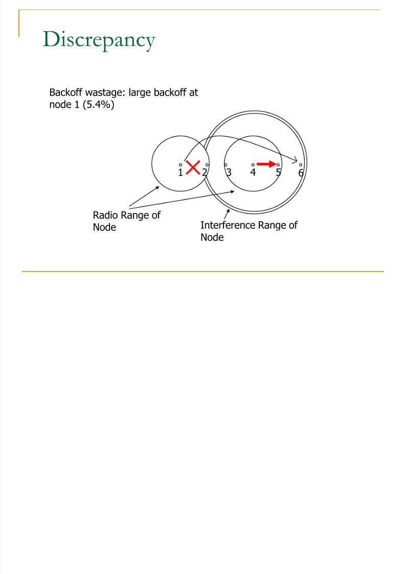
1 2 3 4 6

Radio Range ofNode Interference Range of

Node

5

Discrepancy

Backoff wastage: large backoff atnode 1 (5.4%)

C i f A R l L i

8/13/2019 11 Capacity


Two communication patterns

Scenario #1 Scenario #2

Capacity of A Regular Lattice

Network

C i f A R l L i

8/13/2019 11 Capacity


Scenario #1

Internode Distance = 200 m

Interference radius = 550 m

Every third row can operateWithout interference to give aMaximum throughput of 1/4

Thus flow in such a lattice network is expected (theoretically) to reach 1/12


Network

8/13/2019 11 Capacity



Network

Expected:

(1/12) * 1.7 =

0.14 Mbps

Observed:

0.1 Mbps

Discrepancy:

Same as in chain

C i f A R l L i

8/13/2019 11 Capacity


Scenario #2Traffic flow direction

1) Optimal Scheduling possiblewith predetermined routes.

2) Overall throughput can bemaximized (in theory) with onevertical flow in one time unitand horizontal flows in another

3) Per-flow throughput isexpected to be (1/24)


Network

8/13/2019 11 Capacity


Slightly less than half of the per-flow throughput without crosstraffic

Possible Problem :

Head of queue block


Network

8/13/2019 11 Capacity


Capacity of Random Network

Expect to see similartotal capacity tolattice network

No dramatically loss1) Hole in area

2) Center is moresusceptible tocongestion

8/13/2019 11 Capacity


Traffic Pattern

Random traffic pattern The capacity available to each node is

O(1/sqrt(n))

Scalable traffic pattern Exactly local traffic: fixed distance

Power law distance distribution: if the distancedistribution decays more rapidly than the square

of distance The basic idea is that the average path length in

scalable traffic pattern should be kept constant

8/13/2019 11 Capacity


Impact of Interference on Multi-hop

Wireless Network Performance

Framework to answer questions about thecapacity of specific topologies with specifictraffic pattern

Assumptions No mobility

Fluid model

Centralized scheduler

The basic idea is to model as a standardnetwork flow problem with wirelessconstraints

8/13/2019 11 Capacity


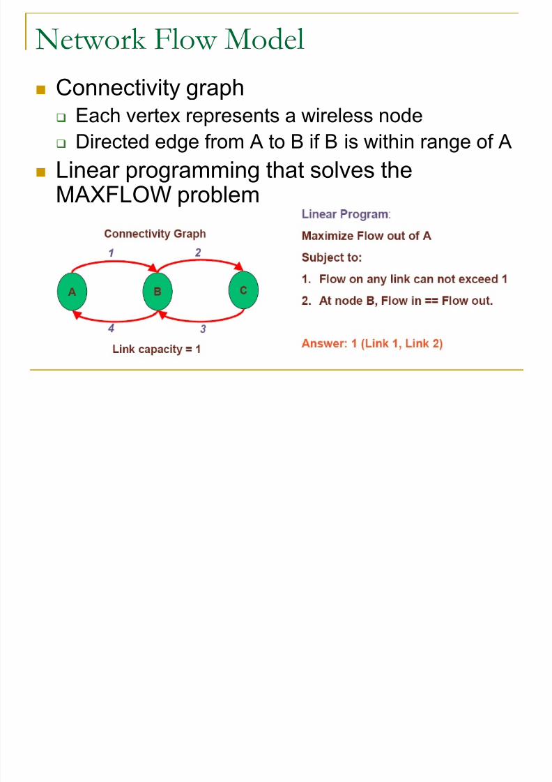
Network Flow Model

Connectivity graph Each vertex represents a wireless node

Directed edge from A to B if B is within range of A

Linear programming that solves the

MAXFLOW problem

f h h

8/13/2019 11 Capacity


Conflict Graph (Contention Graph)

Each edge in the connectivity graph (link)represented by a vertex in conflict graph

An undirected edge between two vertices(links) if one link will interfere with the other

If there are an edge between two links, then thetwo links cannot transmit together

8/13/2019 11 Capacity


Clique Constraints

Cliques in conflict graph At most one link in a clique can be active at any

instance

Augment MAXFLOW LP to get upper bound

f l

8/13/2019 11 Capacity


Properties of Clique Constraints

Finding all cliques takes exponential time

Even if all cliques are found, no optimality is

guaranteed

More cliques added, more tight the bound

Tradeoff between computation and

performance

d d S C i

8/13/2019 11 Capacity


Independent Set Constraints

All links belong to an independent set can beactive together

No two independent sets can active at thesame time

Augment MAXFLOW LP to get lower bound

P i f I d d S C i

8/13/2019 11 Capacity


Properties of Independent Set Constraint

Lower bound is always feasible LP can output a schedule

Finding all independent sets takes

exponential time The lower bound is optimal is all independent sets

are found

Lower bound will increase if we add more

independent sets If upper and lower bound converge, the

optimality is guaranteed

S G li i

8/13/2019 11 Capacity


Some Generalizations

Multiple radio on orthogonal channels

Multiple, non-interfering links between nodes

Directional antenna

Appropriate edges in connectivity graph

Conflict graph can also accommodate

Multiple sender/receiver

Multi-commodity flow problem for LP

R i

8/13/2019 11 Capacity


Routing

Shortest path is not enough

Channel quality should be considered

May introduce congestion

Interference-aware routing Prefer routes that use up minimum amount of

spectrum resource

Advantageous sometimes even with 802.11 MAC

Li i i

8/13/2019 11 Capacity


Limitations

Computation cost

2-5 minutes for ~100 nodes

No guarantee to get optimal schedule in

polynomial time Change in conflict graph

Slow vs. fast change

Fairness is bad

C i f M l i Ch l Wi l

8/13/2019 11 Capacity


Capacity of Multi-Channel Wireless

Networks

Multiple channels share a fixed bandwidth

Consider multiple channels and multiple

interfaces in networks

# of channel c , # of interface m per node

What if we use less interfaces than channels

m < c

Intuitively, capacity degradation may occur

R l

8/13/2019 11 Capacity


Results

The capacity is dependent on the ratio c/m,

and not on the exact value of either c or m

For Arbitrarynetwork:

There is

always acapacity

loss

R l

8/13/2019 11 Capacity


Results

No degradation when c/m = O(log n)

If c = O(log n), then m = 1 suffices

For Random

network:

C it f P C t i d Ad h

8/13/2019 11 Capacity


Capacity of Power Constrained Ad-hoc

Network

Consider model with low spectral efficiency

Arbitrary large bandwidth

Power constrained

Two applications UWB

Sensor network

The result is that throughput increases withnode enter the network

I i i

8/13/2019 11 Capacity


Intuition

SINR = Signal / (Noise + Interference)

Noise = noise density * bandwidth

In bandwidth-constrained scenario, SINR is

dominated by interference In low spectral efficiency, SINR is mainly

affected by ambient noise

Q ti

8/13/2019 11 Capacity


Question:

What are the fundamental limitations of

wireless network?

S mm r F tors Infl en ing C p it

8/13/2019 11 Capacity


Summary – Factors Influencing Capacity

Node placement

Traffic pattern

Static / Mobile

Available Bandwidth

Multi-Channel

Infrastructure support

Directional / Omnidirectional antenna

Th k !

8/13/2019 11 Capacity


Thanks!

Question?

Suggestion?

R f r

8/13/2019 11 Capacity


Reference

P. Gupta and P. R. Kumar, " The capacity of wireless networks,'' IEEETransactions on Information Theory , vol. IT-46, no. 2, pp. 388-404, March 2000

Capacity of power constrained ad-hoc networks , Arjunan Rajeswaran, RohitNegi, IEEE Infocom 2004, Hong Kong, March 2004.

Jinyang Li, Charles Blake, Douglas S. J. De Couto, Hu Imm Lee, and RobertMorris, Capacity of Ad Hoc Wireless Networks, Proceedings of the 7th ACMInternational Conference on Mobile Computing and Networking (MobiCom '01),

Rome, Italy, July 2001, pages 61-69 Kamal Jain, Jitendra Padhye, Venkata N. Padmanabhan, and Lili Qiu. Impact of

Interference on Multi-hop Wireless Network Performance. In Proc. of ACMMOBICOM, San Diego, CA, September 2003

Matthias Grossglauser and David Tse. Mobility Increases the Capacity ofMobile Ad-hoc Wireless Networks. IEEE/ACM Transactions on Networking,Vol. 10, No. 4, Aug. 2002

Pradeep Kyasanur and Nitin Vaidya. Capacity of Multi-Channel WirelessNetworks: Impact of Number of Channels and Interfaces In Proc. of ACMMobiCom 2005, Aug. - Sept. 2005

Abbas El Gamal, James Mammen, Balaji Prabhakar, and Devavrat Shah.Throughput-Delay Trade-off in Wireless Networks. Proc. of IEEE INFOCOM,March 2004.

11 capacity

Documents