10th ebes conference proceedings
TRANSCRIPT
10th EBES CONFERENCE PROCEEDINGS MAY 23-25, 2013 TAKSIM NIPPON HOTEL ISTANBUL, TURKEY
2013
ISBN: 978-605-64002-1-6
PROCEEDINGS OF THE 10th EURASIA BUSINESS AND ECONOMICS SOCIETY CONFERENCE (EBES) - ISTANBUL
MAY 23-25, 2013 TAKSIM NIPPON HOTEL, ISTANBUL, TURKEY
ISBN: 978-605-64002-1-6
10th EBES Conference Proceedings (ISBN: 978-605-64002-1-6)
EBES Publications / EBES Yayınları Mailing Address / Yönetim Yeri Adresi: Akşemsettin Mah. Kocasinan Cad.
Erenoğlu İş Merkezi No: 8/4 34080 Fatih - İstanbul, Türkiye Publication Type / Yayın Türü: E-book / Elektronik Kitap
Istanbul - Turkey / İstanbul - Türkiye August 2013 / Ağustos 2013
The authors of individual papers are responsible for technical, content, and linguistic correctness.
Published by EBES
Copyright © 2013

EBES Eurasia Business and Economics Society
Eurasia Business and Economics Society (EBES) is a scholarly association for scholars involved in the practice and study of economics, finance, and business worldwide. EBES was founded in 2008 with the purpose of not only promoting academic research in the field of business and economics, but also encouraging the intellectual development of scholars. In spite of the term “Eurasia”, the scope should be understood in its broadest term as having a global emphasis. EBES aims to bring worldwide researchers and professionals together through organizing conferences and publishing academic journals and increase economics, finance, and business knowledge through academic discussions. To reach its goal, EBES benefits from its advisory board which consists of well known academicians from all around the world. Last year, with the inclusion of new members, our advisory board became more diverse and influential. I would like to thank them for their support. EBES conferences and journals are open to all economics, finance, and business scholars and professionals around the world. Any scholar or professional interested in economics, finance, and business around the world is welcome to attend EBES conferences. Starting from 2012, EBES organizes three conferences every year: One in Istanbul (possibly in the early summer) and two in Europe or Asia (possibly in January and in fall). In 2011, EBES began publishing two academic journals. One of those journals, Eurasian
Business Review - EBR, is in the fields of industry and business, and the other one, Eurasian
Economic Review - EER, is in the fields of economics and finance. Both journals are
published bi-annually in Spring and Fall and we are committed to having both journals included in SSCI as soon as possible. Both journals are currently indexed in the Cabell's
Directory, Ulrich's Periodicals Directory, IBSS: International Bibliography of the Social
Sciences, RePEc, EBSCO Business Source Complete, ProQuest ABI/Inform, and EconLit. EBES also publishes the EBES Anthology annually to give opportunity for the papers presented at the EBES conferences.

EBES ADVISORY BOARD
• Hassan ALY, Department of Economics, Ohio State University, U.S.A.
• Ahmet Faruk AYSAN, Central Bank of the Republic of Turkey, Turkey
• Jonathan BATTEN, Department of Finance, Hong Kong University of Science &
Technology, Hong Kong
• Michael R. BAYE, Kelley School of Business, Indiana University, U.S.A.
• Simon BENNINGA, The Faculty of Management, Tel Aviv University, Israel
• Idris BIN JAJRI, Faculty of Economics and Administration, University of Malaya, Malaysia
• Wolfgang DICK, ESSEC Business School, France
• Mohamed HEGAZY, School of Management, Economics and Communication, The
American University in Cairo, Egypt
• Heather HOPFL, Essex Business School, University of Essex, UK
• Philip Y. HUANG, China Europe International Business School, China
• Irina IVASHKOVSKAYA, State University - Higher School of Economics, Russia
• Soo-Wook KIM, College of Business Administration, Seoul National University, Korea
• Christos KOLLIAS, Department of Economics, University of Thessaly, Greece
• Ali M. KUTAN, Department of Economics and Finance, Southern Illinois University
Edwardsville, U.S.A.
• William D. LASTRAPES, Terry College of Business, University of Georgia, U.S.A.
• Rita MÅRTENSON, School of Business, Economics and Law, Göteborg University,
Sweden
• Guilherme PIRES, Newcastle Graduate School of Business, University of Newcastle,
Australia
• Panu POUTVAARA, Faculty of Economics, University of Munich, Germany
• Euston QUAH, School of Humanities and Social Sciences, Nanyang Technological
University, Singapore
• Peter RANGAZAS, Department of Economics, Indiana University-Purdue University
Indianapolis, U.S.A.
• J. Mohan RAO, Department of Economics, University of Massachusetts, U.S.A.
• John RUST, Department of Economics, University of Maryland, U.S.A.
• M. Ibrahim TURHAN, Istanbul Stock Exchange, Turkey
• Marco VIVARELLI, Faculty of Economics, Catholic University of Milano, Italy
• Naoyuki YOSHINO, Faculty of Economics, Keio University, Japan
Organizing Committee
Iftekhar Hasan, PhD, Fordham University, U.S.A.
Mehmet Huseyin Bilgin, PhD, Istanbul Medeniyet University, Turkey
Hakan Danis, PhD, Union Bank, U.S.A.
Pascal Gantenbein, PhD, University of Basel, Switzerland
Ender Demir, PhD, Istanbul Medeniyet University, Turkey
Orhun Guldiken, University of Arkansas, U.S.A.
Ugur Can, EBES, Turkey
Merve Aricilar, EBES, Turkey
Reviewers
Sagi Akron, PhD, University of Haifa, Israel
Mehmet Huseyin Bilgin, PhD, Istanbul Medeniyet University, Turkey
Lorenzo Burlon, PhD, Bank of Italy, Italy
Hakan Danis, PhD, Union Bank, U.S.A.
Ender Demir, PhD, Istanbul Medeniyet University, Turkey
Pascal Gantenbein, PhD, University of Basel, Switzerland
Orhun Guldiken, University of Arkansas, U.S.A.
Peter Harris, PhD, New York Institute of Technology, U.S.A.
Gokhan Karabulut, PhD, Istanbul University, Turkey
Chi Keung Marco Lau, PhD, University of Northumbria, United Kingdom
Gregory Lee, PhD, University of the Witwatersrand, South Africa
Nidžara Osmanagić-Bedenik, PhD, University of Zagreb, Croatia Doojin Ryu, PhD, Chung-Ang University, South Korea
Meltem Sengun Ucal, PhD, Kadir Has University, Turkey
R. Baris Tekin, PhD, Marmara University, Turkey
Preface We are excited to organize our 10th conference on May 23rd, 24th, and 25th, 2013 at the Taksim Nippon Hotel in Istanbul, Turkey. We are honored to have received top-tier papers
from distinguished scholars from all over the world. We regret that we were unable to accept more papers than we have. In the conference, 288 papers were presented and 499 colleagues from 58 countries attended the conference. This conference proceeding is our first proceeding that includes selected full papers from the 10th EBES Conference – Istanbul. We have accepted 30 papers among resubmitted full papers after the conference ended. In this proceeding you will find a snapshot of topics that are presented in the conference. As expected, our conference has been an intellectual hub for academic discussion for our colleagues in the areas of economics, finance, and business. Participants found an excellent opportunity for presenting new research, exchanging information and discussing current issues. We believe that this conference proceeding and our future conferences will improve further the development of knowledge in our fields. Distinguished researchers, Iftekhar Hasan, Kose John, and Bill B. Francis joined the conference as keynote speakers. Iftekhar Hasan is the E. Gerald Corrigan Chair in
International Business and Finance at Fordham University's Schools of Business and co-director of the Center for Research in Contemporary Finance. Professor Hasan serves as the scientific advisor at the Central Bank of Finland and as president of the Eurasia Business and Economics Society. He is the managing editor of the Journal of Financial Stability. Kose John is Charles William Gerstenberg Professor of Banking and Finance at Stern School of Business in New York University, USA. He serves as the editor in Advances in Financial Economics and Financial Management. He is also the associate editor in many high ranked journals such as Review of Quantitative Finance and Accounting, International Review of Financial Analysis, the International Journal of Finance, and Journal of Corporate Finance. Bill B. Francis is the Warren H. and Pauline U. Bruggeman Distinguished Professor of
Finance and Director of the PhD Program in Rensselaer Polytechnic Institute in NY, USA. He is currently on the editorial board of many journals including the Journal of Financial Stability. I would like to thank all presenters, participants, board members, and keynote speakers and I am looking forward to seeing you all again at the upcoming EBES conferences. Best regards, Ender Demir, PhD Conference Coordinator
CONTENTS
TITLE AUTHORS PAGE NUMBERS
QUALITY COSTS WITHIN THE FRAMEWORK OF TOTAL QUALITY MANAGEMENT AND A CASE STUDY IN THE CUKUROVA REGION OF TURKEY
VEYIS NACI TANIS, ILKER KEFE 1-12
SUBSTITUTABILITY BETWEEN DRUGS, INNOVATION AND GROWTH IN THE PHARMACEUTICAL INDUSTRY
FELIPA DE MELLO-SAMPAYO, SOFIA DE SOUSA VALE, FRANCISCO CAMOES
13-28
RISK EXPOSURE, RISK-BEARING CAPACITY, AND RISK-COPING STRATEGIES OF URBAN HOUSEHOLDS IN MALAYSIA
SELAMAH ABDULLAH YUSOF, WAN JAMALIAH WAN JUSOH, ROHAIZA ABD ROKIS
29-40
A REVIEW OF IMPACT MAKING TECHNOLOGIES IN SUPPLY CHAIN MANAGEMENT
ARIFUSALAM SHAIKH, MOHAMMAD KHALIFA AL-DOSSARY
41-51
BRIBERY PROBLEMIN KUWAITI ADMINISTRATION: AN EXPLORATORY STUDY
MOHAMMAD QASEM AHMAD AL-QARIOTI 52-64
CYCLICAL FLUCTUATIONS AND CREDIT RISK MANAGEMENT IN ITALY IN THE PERIOD 2008-2012: A BIOSTATISTICAL APPROACH
STEFANO OLGIATI, ALESSANDRO DANOVI
65-74
HOW DID CDS MARKETS IMPACT STOCK MARKETS? EVIDENCE FROM LATEST FINANCIAL CRISIS
HASAN FEHMI BAKLACI, OMUR SUER 75-80
INVESTIGATION OF CAUSAL RELATIONS IN THE ENDOGENOUS MONEY SUPPLY AND ORTHODOX MONETARY THEORY FOR THE USA USING IV AND GMM
AZRA DEDIC 81-96
THE INFLUENCE OF CAPITAL STRUCTURE ON FINANCIAL PERFORMANCE: EVIDENCE FROM ROMANIAN MANUFACTURING COMPANIES
SORANA VATAVU 97-107
THE INTEGRATION AND CONCENTRATION/SPECIALIZATION OF EUROPEAN COUNTRIES ACROSS MANUFACTURING INDUSTRIES
SEYIT KOSE, AYKUT SARKGUNESI
108-129
CVaR-E(r) EQUILIBRIUM ASSET PRICING
MIHALY ORMOS, DUSAN TIMOTITY
130-153
CULTURAL OPENNESS AS A FACTOR OF BUILDING CREATIVE REGION: WROCLAW COMPARED TO OTHER POLISH CITIES
MALGORZATA NIKLEWICZ-PIJACZYNSKA, MALGORZATA WACHOWSKA
154-171
BUILDING A LEARNING ORGANIZATION: DO LEADERSHIP STYLES MATTER?
NORASHIKIN HUSSEIN, NOORMALA AMIR ISHAK, FAUZIAH NOORDIN
172-180
AIR TRAFFIC DELAYS, SAFETY, AND REGULATOR’S OBJECTIVES: A MONOPOLY CASE
CHUNAN WANG
181-200

CORPORATE GOVERNANCE DISCLOSURE: A CASE OF BANKS IN MALAYSIA
NASUHA NORDIN, MOHAMAD ABDUL HAMID
201-216
IMPORTANCE AND ROLE OF SOCIAL MATURITY IN THE CONCEPT OF HOLISTIC MANAGERIAL COMPETENCE
JAN PORVAZNIK, JURAJ MISUN 217-232
THE EFFECTS OF THE 2007-2008 FINANCIAL CRISIS ON TURKISH FIRMS
EMINE EBRU AKSOY, ERGINBAY UGURLU 233-241
CHINA’S APPEARING ON THE HORIZON AND THE CHANGING PATTERN OF GLOBAL ECONOMY
XUHENG ZANG, YANG LI, YANG HE 242-259
ANALYSIS OF RISK IN ISLAMIC AND CONVENTIONAL BANKING: SURVEY ON BAHRAIN, THE UNITED ARAB EMIRATES AND MALAYSIA
NORAZWA AHMAD ZOLKIFLI, MOHAMAD ABDUL HAMID, NOOR INAYAH YA’AKUB
260-270
GENDER AND HOUSEHOLD EDUCATION EXPENDITURE IN TURKEY
Z. BILGEN SUSANLI 271-281
STRATEGIC INNOVATION IN POLISH TRANSPORT INDUSTRY
BEATA SKOWRON-GRABOWSKA
282-287
FRANCHISING BETWEEN CONTROL AND AUTONOMY: WHAT IMPACTS ON INNOVATION?
KERIM KARMENI, OLIVIER DE LA VILLAREMOIS, FAYSAL MANSOURI
288-301
NON-EU EURASIA INVESTMENT FOR RESIDENCE: THE LATVIAN WAY
ANDREJS LIMANSKIS 302-318
A STUDY ON STAKEHOLDER MODEL CHANGE AND SOCIAL RESPONSIBILITY TYPE FOR FOXCONN IN CHINA
BYUNG HUN CHOI 319-338
MOBBING IN ORGANIZATIONS
NEVRA SANIYE GUL, A. TUGBA KARABULUT
339-345
SYSTEM MODELING OF REGIONAL ECONOMIC PROCESSES DYNAMIC ON THE BASE OF THE INFORMATION MODELLING TECHNOLOGY
ALEXANDRE BOULYTCHEV, VLADIMIR BRITKOV
346-354
SOVEREIGN WEALTH FUND INVESTMENTS IN THE BANKING INDUSTRY
ANDERLONI LUISA, VANDONE DANIELA 355-374
THE KNOWLEDGE ECONOMY İN THE WESTERN BALKAN COUNTRİES AND TURKEY
SHENAJ HADZIMUSTAFA, GADAF REXHEPI, SADUDIN IBRAIMI, NEXHBI VESELI
375-391
ITALIAN GOVERNMENT BONDS: AN EMPIRICAL STUDY
GABRIELLA FOSCHINI, SILVIA BUTTARAZZI, FRANCESCA FRANCETTI
392-415

THE GOODNESS OF MOVING AVERAGE CONVERGENCE DIVERGENCE AND RATE OF CHANGE INDICATORS IN SECURING THE STOCK RETURN: A STUDY OF COMPANY INDICES IN BURSA MALAYSIA
MUHAMAD SUKOR JAAFAR, ISMAIL AHMAD, SAIFUL HAFIZAH JAAMAN
416-424
10th EBES Conference Proceedings 23 - 25 May, 2013. NIPPON HOTEL, ISTANBUL, TURKEY ISBN: 978-605-64002-1-6. WEBSITE: www.ebesweb.org
* Acknowledgements: We would like to thank Fiona Orel for grammar checking. This work is supported by the Research Fund of Cukurova University, Adana, Turkey, under grant contracts no. IIBF2013YL4.
1
QUALITY COSTS WITHIN THE FRAMEWORK OF TOTAL QUALITY MANAGEMENT AND A CASE STUDY IN THE
CUKUROVA REGION OF TURKEY*
VEYIS NACI TANIS Department of Business
Cukurova University Turkey
ILKER KEFE Department of Business
Cukurova University Turkey
[email protected] Abstract: Resources of an enterprise are mainly used at pre-production, in process, and
post-production after delivery of products to customers. With the increasing competition, the importance of efficient use of resources and quality costs concepts has emerged. The quality cost concepts that have recently been widely used by businesses makes a contribution to a company’s productivity. In this study, a bus and midibus production company is chosen and, there is an analysis of its quality costs and its efforts to decrease quality costs. This paper illuminates the efforts to introduce and implement quality cost measures’ by one automobile manufacturer, and is a real life case analysis. The costs that existed in production are shown in this study. The methodology adopted here is the implementation of a case analysis. The Company has a production period and several steps for a productive production process. The quality cost report is prepared monthly, once every six months and annually; and there is comparison of the quality cost variations of every quality cost element, such as scrap, rework, warranty expenses, and service modifications. The company also particularly focuses on failure costs (nonconformance costs), and performs works or studies to decrease these costs. Keywords: Quality, Quality Costs 1. INTRODUCTION 1.1. Meaning of quality and total quality management Many companies are undergoing rapid and significant changes in today’s business world. Global competition operates under a technology ‘push’ and market ‘pull’ system, so organizations have to compete on speed of delivery, price, level of technology and quality dimensions (Sharma et al. 2007). Nowadays, quality studies are not only the responsibility of a small group people who monitor performance and remove defective products from assembly lines. It is essential that all initiatives for the procurement of quality are considered, and quality must involve the whole organization in a drive for continuous improvement (Jafar et al. 2010). The term quality has many meanings:

10th EBES Conference Proceedings
2
A degree of excellence Conformance with requirements Fitness for use Fitness for purpose Freedom from defects, imperfections and contamination Satisfaction of needs Delighting customers
Juran (1951) has proposed a definition of quality as being “fitness for use” (fitness is to be defined by the customer). Crosby (1979) defines quality as “conforming to specifications” (The weakness of this definition is that the specifications may not be what the customer wants or is willing to accept). Soin (1993) defines quality as products and services that meet or exceed customers’ expectations.
Quality activities first began with inspection and testing, and these continued to be the only departmental activities until the 1950s (Juran et al. 1951). Following this, quality improved
with quality control, quality assurance and total quality management approaches. Without certain principles, achieving a common understanding in the field of quality management would be impossible, and in the 1950s, Juran et al. (1951) introduced the concept of quality
management and defined principles of rules, regulations, instructions and requirements (Hoyle, 2011). Total Quality Management (TQM) is now used by businesses because it improves quality. TQM is both a culture, and a set of strategic principles for the continuous improvement of organizations (Jafar et al. 2010). TQM facilities include production features
as well as production systems. For automobile manufacturers, these features include antilock brakes, safety air bags, sun and moon roofs, and quiet operation. It is also important that these features are provided at a reasonable price. Japanese automobiles are striking examples. Their attractive quality features are threatening other luxury car producers such as Mercedes Benz and BMW. The same concept can be applied to all products and services (Soin, 1993). Because of national and international competition on one hand, and rapidly changing technology on the other, Total Quality Management practices which lead to better recognition and productive discussions could be useful and effective (Jafar et al. 2010).
This paper discusses quality costs and management’s role regarding quality costs. There is an initial brief overview of the recent history of quality costs and quality cost approaches. Following this, a case study is introduced that exemplifies how quality costs are calculated and evaluated in an automobile company. 1.2. Quality costs Managers need to make effective use of monetary resources, and quality costing is one reliable tool for the evaluation of efficiency and effectiveness of companies’ financial systems. It is a measure for quality promotion and a basis for all decisions referring to quality (Andrijasevic, 2008). By establishing a total quality management system and identifying the quality costs of the organization, a company can move towards reducing these costs within the system, improving services and producing better quality than before. This will lead to an improved quality process and more effective Total Quality Management (Jafar et al. 2010).
Quality related costs are not limited to the departments of an organization, but also include subcontractors, suppliers, stockists, agents and dealers. In addition, customers can be affected by quality related costs (De, 2009). There are three fundamental causes of poor quality, and it is important to identify and measure the costs (De, 2009).

10th EBES Conference Proceedings
3
Investing in the prevention of nonconformance to requirements, appraising a product or service for conformance to requirements, and failing to meet requirements are all quality costs (Akhade and Jaju, 2009). The term “quality cost” has been defined in several ways. For example (Juran et al., 1951):
The cost of attaining quality. The costs of running the quality department. The costs of finding and correcting defective work. The cost of ensuring and assuring as well as loss incurred when quality is not
achieved (BS6143 Part 2).
Andrijasevic (2008) indicates that a quality-costing approach is based on two fundamental conditions:
Quality must be measurable by money. There must be a cause and effect relationship between quality and financial
outcomes.
Quality related costs emerge in a wide range of activities and involve all the departments in an organization, such as sales and marketing, design, research and development, purchasing, storage and handling, production planning and control, manufacturing/operations, delivery, installation, service, finance and accounts (De, 2009).
According to the traditional Prevention, Appraisal and Failure (P-A-F) model, Juran (1951) and Feigenbaum (1956) classify quality costs into prevention, appraisal, and failure (internal and external failures) costs. Juran (1979) describes a model that gives “optimum quality costs”. The quality cost data attract the attention of the management, and provide the incentive to begin a quality improvement programme. The resulting improvements in quality lead to perfection and customer satisfaction, which result in increased market share and profits (Juran, 1951). Crosby (1979) classifies cost of quality as “price of conformance and nonconformance”. Conformance costs consist of appraisal and prevention costs; nonconformance costs consist of internal and external costs.
Prevention costs are costs that keep defects from occurring in the first place (Feigenbaum, 1956), and are investments that help to reduce future appraisal and failure costs (Grottke and Graf, 2009). Appraisal costs are expenses incurred to maintain the company, period and product quality; and check whether a product or service meets its quality requirements. Failure costs are costs that are caused by defective materials and products (Feigenbaum, 1956), and are due to an ineffective quality process in products and services before or after delivery to purchaser (Schiffauerova and Thomsan, 2006). Internal failure costs are costs incurred when materials or products do not meet the standard specifics. They can occur prior to delivery or shipment of the product, or during the furnishing of a service to the customer. External failure costs are costs incurred after delivery or shipment of the product, and during or after furnishing of the service to the customer (Wu et al. 2011; Desai, 2007). Table 1 shows principal prevention, appraisal, internal and external failure cost components.
Most companies are not aware of the true cost of quality (Yang, 2008). The cost of quality model has two principal concepts (Kump, 2006):
The total cost of quality is the cost of the effort to eliminate errors and defects,
plus the cost of defects that remain.

10th EBES Conference Proceedings
4
Prevention costs less than design review; design review less than inspection or quality cost; inspection or quality cost less than letting the defect reach the customer.
Table 1: Quality costs
QUALITY COSTS
PREVENTION COSTS - Quality planning - Process planning - Designing and process controlling - New-product review - Supplier quality evaluation - Training - Quality audits - Reporting APPRAISAL COSTS - Creating quality systems and their audits - Incoming inception and test - In-process inception and test - Final inception and test - The end product quality audits - Evaluation of sub-contractor - Controlling inception and measurement equipment - Inception and test materials and services - Evaluation of stocks
INTERNAL FAILURE COSTS - Scrap - Rework - Re-inception - Retest - Failure analysis - One hundred percent sorting inception - Avoidable process losses - Unsuitable preservation of raw materials - Retesting the modified items - Classifying product quality under the acceptable level - Downgrading -scrap and rework- supplier - Maintenance and duplication of the manufactured products - Repairing and modifying received defected items EXTERNAL FAILURE COSTS - Warranty charges - Product return by customers and their complaints - Modification of the products delivered to customers - Allowances
Source: Jafar et al. (2010); Tanis (2005); Juran et al. (1951)
Quality costing is one of the several tools and techniques which help companies to improve quality of product and service. It is possible to solve 95% of problems with quality tools. (De, 2009). Quality costs (especially external failures) can have the following consequences in terms of customer behavior (Soin, 1993):
For every customer who bothers to complain, there are 26 others who remain
silent. The average “wronged” customer will tell 8 to 16 people (over 10 percent tell
more than 20 people). Unsatisfied customers (91%) will never purchase goods or services from the
business again.
However, if companies make an effort to remedy customer complaints, 82 to 95 percent of customers who have had a bad experience can be retained. Attracting a new customer costs 5 times more than retaining an existing one. Companies who have high quality costs (especially external failure costs) are more likely to have unsatisfied customers who will probably not make any further purchase.
In general, the literature reports quality costs to be between 5 and 30% of sales (Giakatis et al. 2001). Feigenbaum (1956) specifies in one Total Quality Control study that quality cost
expenditures represent between 7 and 10% of cost of sales. Desai (2008) has also stated

10th EBES Conference Proceedings
5
that the cost of quality of a company runs in the range of 5 to 35% revenue for manufacturing organizations, or 25 to 40% of operating expenses for service organizations (Desai, 2008). Companies that know how to conduct effective quality planning and control can manage to reduce their quality cost from 36% to only 3% of sales in several years (Andrijasevic, 2008). Some organizations do not include the prevention costs in their quality costing reporting system, they only collect and report the cost of failure and appraisal. Analysis of failure costs which have functional causes (e.g. production, purchasing, and marketing) is not usually readily available (De, 2009). One way to reduce these product-related costs is by reducing costs of quality. Therefore, to recognize, classify, and improve these costs must be important for all companies (Jafar et al. 2010).
Several authors also propose cost of quality models that include prevention, appraisal and failure costs, conformance and nonconformance costs, intangible costs and opportunity costs. Numerous studies on quality costing have been undertaken in different areas such as manufacturing, construction, building, and highway engineering. Some of these studies are listed in Table 2 (Sharma et al. 2007).
Table 2: Studies in the literature
Year Author Area 1994 Carr and Ponoemon Paper and pulp industry 1995 Abdul-Rahman Highway engineering 1995 Israeli and Fisher General 1995 Willis and Willis Process quality 1996 Campanella General 1999 Harrington General 1999 Josephson and Hammarlund Building 2000 Zhao General 2001 Roden and Dale Engineering company 2002 Dale and Wan Engineering company 2003 Lai and Cheng Manufacturing company 2004 Omachonu and Suthumannon Manufacturing company
Source: Sharma et al. (2007)
Newer research, such as Schiffauerova and Thomsan’s study (2006), shows that just one of four multinational companies has a formal cost of quality methodology and uses systematic quality initiatives. They explain that a cost of quality approach is not utilized in most quality management programs.
Liu et al. (2008) propose a new model for cost of quality based on the Activity Based Costing
(ABC) method in a Computer Integrated Manufacturing System (CIMS) environment. The ABC cost assignment method facilitates cost of quality analysis and control. Yang (2008) has stated that certain costs are difficult to identify and quantify. These so-called “hidden” quality costs have two subdivisions: extra resultant costs and estimated hidden costs.
Desai (2008) investigates quality costs in small and medium enterprises and calculates present and future budgeted quality costs. The study aims to identify hidden costs, analyze them, eliminate them at the roots, relate quality expenditure to various business performance measures and create a budget for the following year.
Grottke and Graf’s study (2009) provides a six-step procedure for assessing, structuring and modeling software failure costs, and aims to predict future failure costs. In the study,
10th EBES Conference Proceedings
6
prediction capabilities allow improved cost-driven planning and control of software projects, and the approach could help in adequately allocating resources.
Jia and Gong (2009) report that they are only concerned with the relationship between the internal factors of quality costs, not the external factors. They developed a new mathematical model for quality costs and adopted the Particle Swarm Optimization (PSO) algorithm to arrive at a solution. They found that the optimization model of cost of quality based on strategic coordination is a valuable and practical model.
Zhang et al. (2009) studied organizational complexity’s effect on quality costs and found that the number of work types has the strongest impact on total quality cost, followed by the number of equipment types, structural complexity, and the number of process steps. They also found that the complexity of division of labor and production technologies have an important effect on quality cost. They suggest that companies should simplify their structure, reduce division of labor, and use high technology equipment to reduce the number of equipment types. 1.3. Management’s role Quality costing provides tools which enable management to obtain detailed information and desirable control, and assists with decision-making processes (Jafar et al., 2010: 24).
Ishikawa (1982) states that these tools are checklists, check sheets, data collection, Pareto diagrams, cause and effect diagrams, stratification, graphs and histograms, scatter diagrams and control charts. Ishikawa (1982) argues that workplace problems can be solved using these tools (Soin, 1993). For products and services, there are three main parameters that determine their salability. They are quality, delivery and price. Customers require products and services of determinate quality to be delivered by or be available by a requested time and to be of a price that reflects value for money. These are customer requirements. Products and services that conform to customer requirements are thought to be products of acceptable quality (Hoyle, 2011). It is crucial that management ensures that the design, production, marketing, and product meet the customer’s needs (Soin, 1993). Quality affects companies both internally and externally (Soin, 1993).
Internally -Higher productivity -Lower prices (competing on price) -Lower costs Externally -Increased customer satisfaction -Increased customer loyalty -More repeat purchases -Increased market share -Higher profits
Organizations exist to achieve a goal, mission or objective; and they must meet the needs, requirements and expectations of their stakeholders. Customers (one of the stakeholders) will be satisfied only if organizations provide products and services that meet their needs, requirements, and expectations (Hoyle, 2011). It is advisable to have a 3 to 5 year company plan. The long-range plan should have the following steps and areas (Soin, 1993):
Company’s or organization’s purpose and vision Customer needs, issues, and channels of distribution Competitive situation
10th EBES Conference Proceedings
7
Products and services Development of partners and purchase plan Financial analysis Potential problem analysis Five year plan Annual plans
Having a quality philosophy helps achieve increased sales, increased productivity, and increased profits. Quality is the key for companies’ survival, success, and prosperity (Soin, 1993). Crosby (1979) states that quality is free. He stresses that if companies eliminate all activity errors and reach zero defects, they can reduce activity costs and increase the level of customer satisfaction (Hoyle, 2011). Therefore, management’s leadership methods, communication between managers, reward types, decision-making and the recording and reporting of quality costs must be redesigned as part of TQM. This is vital in order to compete in today’s global industrial environment (Jafar et al. 2010).
2. RESEARCH AIM There are many automobile, bus and midibus producers such as Mercedes, Isuzu, BMC, and Temsa worldwide. Effectiveness in this sector can be achieved through efforts expended in quality engineering and management. Furthermore, the cost of the quality system is regarded as one of the most efficient performance measurement techniques and arrangement systems.
This paper illuminates the efforts to introduce and implement cost of quality in the automobile industry and is a real life case analysis. The costs that are present during production are shown in this study. The methodology adopted here was the implementation of a case analysis. In the study, the cost of quality budget of the company was investigated and compared with the quality costing approaches and the company’s quality costing method. An interview was conducted with the company’s quality assurance supervisor, and information was obtained about production systems in different areas of the company. 2.1. Introduction to the subject of the study The company selected for this study is a bus and midibus producer that produces for the domestic and international market. The major customers are municipalities, and the firms that provide intercity and intracity transport to the public and companies. The operation is mainly production and assembly. There are some models of entity-specific value; some of these models can vary by country or region and have different specifications. It is possible that designs and specifications demanded by the customers are met, such as a toilet on a bus, or televisions and sound systems. This shows that they are capable of providing a solution to the special needs of any customer by modifying standard products and creating specific and unique products. More than of half the company’s output is exported to Europe. 2.2. Methodology
The objective of this research was to obtain and analyze data from a company in the automobile industry in Turkey. The main interest was to investigate whether the company collects, measures and monitors quality costs; which kinds of costs were considered as quality costs; and whether the collection, measurement and monitoring of the company’s system is suitable for any formal cost of quality approaches; as well as identification of the production process steps. The company is a bus and midibus producer and has a complex

10th EBES Conference Proceedings
8
production system. Some of the parts for manufacturing buses and midibuses are produced by the company; while some are bought from suppliers. The company produces for both internal and external customers. The company’s quality cost model is similar to the general approach (PAF Model). However, the company particularly focuses on failure costs (internal and external cost) and reports these to senior management. The company has a quality improvement program that includes continuous improvement, and focuses on the process, as well as providing extensive education and training on quality for employees. Table 3 shows quality cost facilities.
Table 3: Example of activity costs in the company
Activity – primary Cost of Quality Category
Quality performance reporting Prevention Quality control engineering Prevention Test and audit Appraisal - Prevention Training Prevention Laboratory acceptance test Appraisal Product development Prevention Manufacturing tools Prevention Incoming quality control Appraisal Measuring equipment Appraisal Product defect Failure – Internal Internal quality issues Failure – Internal External quality issues Failure – External
The factors that cause quality problems and costs are pooled by the company’s information system. These data are in information forms on the electronic system, and in paper form. Some of these forms are Deviation Evaluation, Internal Notification, Customer Complaint, Supplier Complaint, Scrap Evaluation
The company uses Pareto diagrams, cause and effect analysis, ratio analysis, and trend analysis to identify quality costs. Managers discuss the quality cost data of the company at the Quality Council. 2.3. Analysis and results The company has a production period and has steps for a productive production process. These steps can have differences according to production of bus and midibus type or model. Standard production process steps of buses and midibuses are Main body production process, Paint process, Mechanical process, Electrical process, Trim process
In the literature, quality costs are divided into four elements: prevention, appraisal, internal and external failure. Crosby (1979) also offers two further divisions of conformance and nonconformance costs. The company particularly focuses on nonconformance costs, and has two main quality ratings. These are to measure non-conformities (scrap, rework etc.), and poor adherence to specifications (internal, external, customers, suppliers). The company gives importance to internal and external quality costs, and adds the other expenditure items such as prevention and appraisal costs to external failures. Therefore, the company only takes notice of nonconformance costs, and adds some conformance costs to internal failure costs as nonconformance costs. The company divides quality costs into three categories according to how quality costs appear. These are: design, production, and supplier problems. These problems affect purchasing, the production process, the costs that occur after sale, and the costs incurred during the guarantee period. These costs can occur when design
10th EBES Conference Proceedings
9
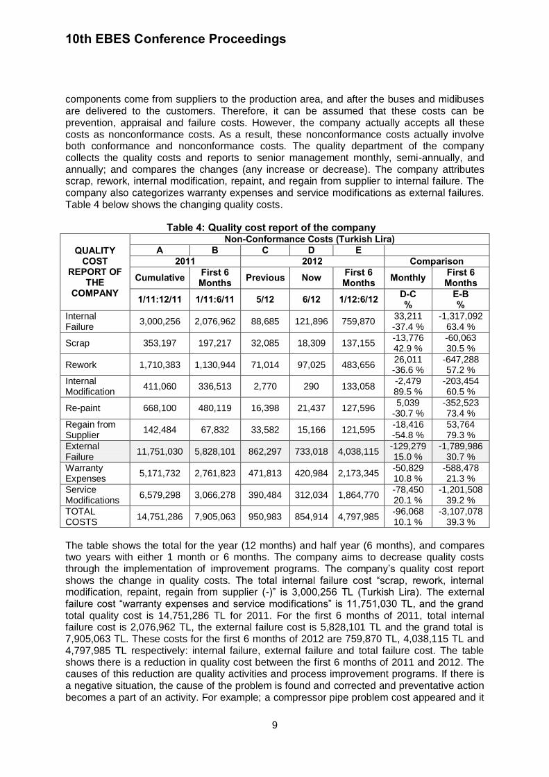
components come from suppliers to the production area, and after the buses and midibuses are delivered to the customers. Therefore, it can be assumed that these costs can be prevention, appraisal and failure costs. However, the company actually accepts all these costs as nonconformance costs. As a result, these nonconformance costs actually involve both conformance and nonconformance costs. The quality department of the company collects the quality costs and reports to senior management monthly, semi-annually, and annually; and compares the changes (any increase or decrease). The company attributes scrap, rework, internal modification, repaint, and regain from supplier to internal failure. The company also categorizes warranty expenses and service modifications as external failures. Table 4 below shows the changing quality costs.
Table 4: Quality cost report of the company
QUALITY COST
REPORT OF THE
COMPANY
Non-Conformance Costs (Turkish Lira) A B C D E
2011 2012 Comparison
Cumulative First 6 Months Previous Now First 6
Months Monthly First 6 Months
1/11:12/11 1/11:6/11 5/12 6/12 1/12:6/12 D-C %
E-B %
Internal Failure
3,000,256 2,076,962 88,685 121,896 759,870 33,211 -37.4 %
-1,317,092 63.4 %
Scrap 353,197 197,217 32,085 18,309 137,155 -13,776 42.9 %
-60,063 30.5 %
Rework 1,710,383 1,130,944 71,014 97,025 483,656 26,011 -36.6 %
-647,288 57.2 %
Internal Modification
411,060 336,513 2,770 290 133,058 -2,479 89.5 %
-203,454 60.5 %
Re-paint 668,100 480,119 16,398 21,437 127,596 5,039
-30.7 % -352,523 73.4 %
Regain from Supplier
142,484 67,832 33,582 15,166 121,595 -18,416 -54.8 %
53,764 79.3 %
External Failure
11,751,030 5,828,101 862,297 733,018 4,038,115 -129,279 15.0 %
-1,789,986 30.7 %
Warranty Expenses
5,171,732 2,761,823 471,813 420,984 2,173,345 -50,829 10.8 %
-588,478 21.3 %
Service Modifications
6,579,298 3,066,278 390,484 312,034 1,864,770 -78,450 20.1 %
-1,201,508 39.2 %
TOTAL COSTS
14,751,286 7,905,063 950,983 854,914 4,797,985 -96,068 10.1 %
-3,107,078 39.3 %
The table shows the total for the year (12 months) and half year (6 months), and compares two years with either 1 month or 6 months. The company aims to decrease quality costs through the implementation of improvement programs. The company’s quality cost report shows the change in quality costs. The total internal failure cost “scrap, rework, internal modification, repaint, regain from supplier (-)” is 3,000,256 TL (Turkish Lira). The external failure cost “warranty expenses and service modifications” is 11,751,030 TL, and the grand total quality cost is 14,751,286 TL for 2011. For the first 6 months of 2011, total internal failure cost is 2,076,962 TL, the external failure cost is 5,828,101 TL and the grand total is 7,905,063 TL. These costs for the first 6 months of 2012 are 759,870 TL, 4,038,115 TL and 4,797,985 TL respectively: internal failure, external failure and total failure cost. The table shows there is a reduction in quality cost between the first 6 months of 2011 and 2012. The causes of this reduction are quality activities and process improvement programs. If there is a negative situation, the cause of the problem is found and corrected and preventative action becomes a part of an activity. For example; a compressor pipe problem cost appeared and it
10th EBES Conference Proceedings
10
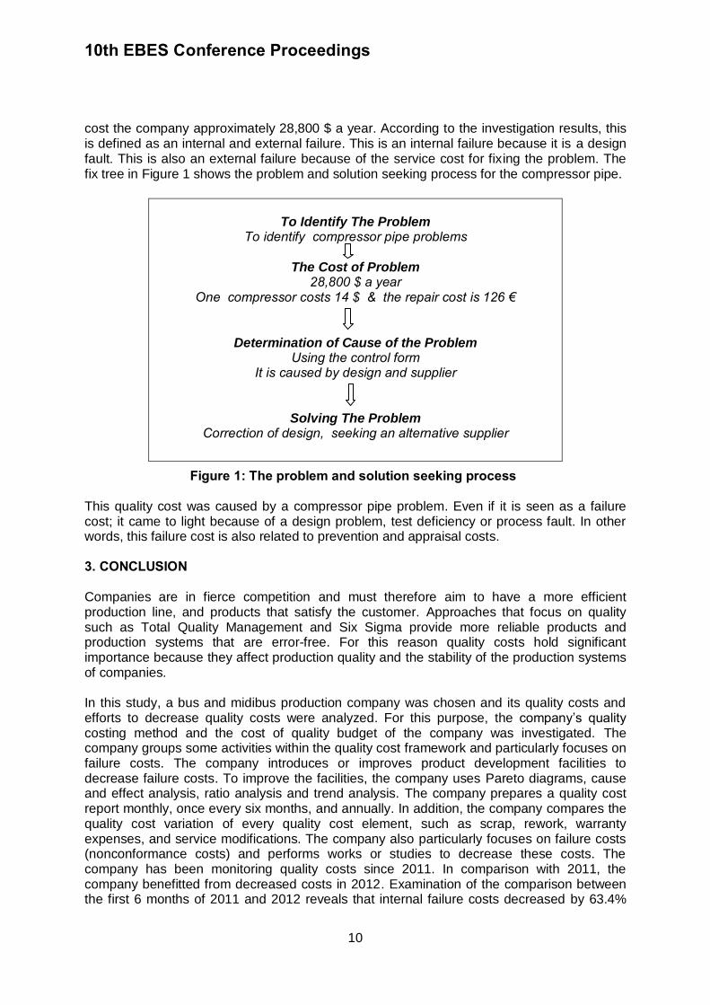
cost the company approximately 28,800 $ a year. According to the investigation results, this is defined as an internal and external failure. This is an internal failure because it is a design fault. This is also an external failure because of the service cost for fixing the problem. The fix tree in Figure 1 shows the problem and solution seeking process for the compressor pipe.
Figure 1: The problem and solution seeking process
This quality cost was caused by a compressor pipe problem. Even if it is seen as a failure cost; it came to light because of a design problem, test deficiency or process fault. In other words, this failure cost is also related to prevention and appraisal costs.
3. CONCLUSION Companies are in fierce competition and must therefore aim to have a more efficient production line, and products that satisfy the customer. Approaches that focus on quality such as Total Quality Management and Six Sigma provide more reliable products and production systems that are error-free. For this reason quality costs hold significant importance because they affect production quality and the stability of the production systems of companies.
In this study, a bus and midibus production company was chosen and its quality costs and efforts to decrease quality costs were analyzed. For this purpose, the company’s quality costing method and the cost of quality budget of the company was investigated. The company groups some activities within the quality cost framework and particularly focuses on failure costs. The company introduces or improves product development facilities to decrease failure costs. To improve the facilities, the company uses Pareto diagrams, cause and effect analysis, ratio analysis and trend analysis. The company prepares a quality cost report monthly, once every six months, and annually. In addition, the company compares the quality cost variation of every quality cost element, such as scrap, rework, warranty expenses, and service modifications. The company also particularly focuses on failure costs (nonconformance costs) and performs works or studies to decrease these costs. The company has been monitoring quality costs since 2011. In comparison with 2011, the company benefitted from decreased costs in 2012. Examination of the comparison between the first 6 months of 2011 and 2012 reveals that internal failure costs decreased by 63.4%
To Identify The Problem
To identify compressor pipe problems
The Cost of Problem
28,800 $ a year One compressor costs 14 $ & the repair cost is 126 €
Determination of Cause of the Problem Using the control form
It is caused by design and supplier
Solving The Problem Correction of design, seeking an alternative supplier
10th EBES Conference Proceedings
11
(The amount is 1,317,092 TL), external failure costs decreased by 30.7% (The amount is 1,789,986 TL), and the total failure costs decreased by 39.3% (The total amount is 3,107,078 TL).
The results of this study show that there is a positive effect of quality improving works on quality costs. Another finding is that monitoring quality costs and cost studies do not actually increase operating costs, and important cost advantages are gained. However, it should be noted that the study is limited in several ways. First, the study is conducted in only one company and sector. Secondly, the company employees are wary of giving latest quality cost data. Further research in this field might investigate a more broad range of companies, sectors, and analyze cost data over a longer period of time.
REFERENCES Akhade, G.N. and Jaju, S.B., 2009. Development of methodology for collecting quality cost in technical institute. In: ICETET-09 Second International Conference on Emerging Trends in Engineering and Technology. Nagpur, India 16-18 December 2009. Andrijasevic, M., 2008. Total quality accounting. Economic Annals, 53(176), pp.110-122.
Crosby, P.B., 1979. Quality is free: The art of making quality certain. New York: McGraw Hill
Custom Publishing. De, R.N., 2009. Quality costing: An efficient tool for quality improvement measurement. In: IE&EM '09 16th International Conference on Industrial Engineering and Engineering Management. Beijing 21-23 October 2009.
Desai, D.A., 2008. Cost of quality in small-and medium- sized enterprises: Case of an indian engineering company. Product Planning & Control, 19(1), pp.25-34.
Feigenbaum, A.F., 1956. Total quality control. Harvard Business Review, 34(6), pp.93-101. Giakatis, G., Enkowa, T., and Washitani, K., 2001. Hidden quality costs and the distinction between quality costs and quality loss. Total Quality Management, 12(2), pp.179-190. Grottke, M. and Graf, C., 2009. Modeling and predicting software failure costs. In: 33rd 2009 Annual IEEE International Computer Software and Applications Conference. Seattle, Washington USA 20-24 July 2009. Hoyle, D., 2011. Quality management essentials. New York: Routledge.
Ishikawa, K., 1982. Guide to quality control, Second revised English Edition. Tokyo: Asian
Productivity Organization. Jafar, A., Taleghani, M., Esmaielpoor, F., and Gudarzvand, C.M., 2010. Effect of the quality system on implementation and execution of optimum total quality management. International Journal of Business and Management, 5(8), August 2010, pp.19-26.
Jia, Z. and Gong, L., 2009. The study of quality costs optimization based on particle swarm optimization algorithm and strategic coordination. In: 2009 Fifth International Conference on Natural Computation. Tianjian, China 14-16 August 2009. USA: IEEE Press Piscataway.

10th EBES Conference Proceedings
12
Juran, J.M. and Godfrey, A.B., 1979. Juran’s quality control handbook. Fifth Edition, New
York: McGraw-Hill. Juran, J.M., Gyrna, F.M., and Bungam, R.S., 1951. Juran’s quality control handbook. New York: McGraw-Hill. Kemp, S., 2006. Quality management demystified. New York: McGraw-Hill. Liu, X., Cui, F., Meng, Q., and Pan, R., 2008. Research on the model of quality cost in CIMS environment. In: IEEE 2008 International Seminar on Business and Information Management. Wuhan, China 19 December 2008. USA: IEEE Computer Society Press.
Schiffauerova, A. and Thomsan, V., 2006. Managing cost of quality: Insight into industry practice. The TQM Magazine, 18(5), pp.542-550. Sharma, R.K., Kumar, D., and Kumar, P., 2007. Quality costing in process industries through QCAS: A practical case. International Journal of Production Research, 45(15), pp.3381-3403. Soin, S.S., 1993. Total quality control essentials. New York: McGraw-Hill. Tanis, V.N., 2005. Teknolojik değişim ve maliyet muhasebesi [Technological change and cost accounting]. Adana: Nobel Kitabevi.
Wu, H., Chien, F., Lin, Y., and Yange, S., 2011. Analysis of critical factors affecting the quality cost of process management of six sigma project based on BSC. International Research Journal of Finance and Economics, 71, pp.92-104. Yang, C.C., 2008. Improving the definition and quantification of quality costs. Total Quality Management, 19(3), pp.175-191.
Zhang, Z., Qin, H., and Wang, L., 2009. A measurement of organizational complexity and its impact on quality economics: A grey perspective. Proceedings of 2009 IEEE Conference on Grey Systems and Intelligent Services, November 10-12, Nanjing, China, pp.783-787.
10th EBES Conference Proceedings 23 - 25 May, 2013. NIPPON HOTEL, ISTANBUL, TURKEY ISBN: 978-605-64002-1-6. WEBSITE: www.ebesweb.org
* Financial support from FCT under grant PTDC/EGE-ECO/104157/2000/ and under BRU-UNIDE is gratefully acknowledge.
13
SUBSTITUTABILITY BETWEEN DRUGS, INNOVATION AND GROWTH IN THE PHARMACEUTICAL INDUSTRY*
FELIPA DE MELLO-SAMPAYO
Department of Economics ISCTE-IUL Portugal
SOFIA DE SOUSA VALE Department of Economics
ISCTE-IUL Portugal
FRANCISCO CAMOES Department of Economics
ISCTE-IUL Portugal
Abstract: This paper establishes a relationship between the elasticity of demand for pharmaceutical intermediates and the growth rate for these intermediates variety. We build a model that contains two sectors, one final good sector producing treatments, and one intermediate goods sector producing a differentiated input used in the final treatment. The effects on the medicaments varieties' growth rate of the introduction of a fiscal instrument over pharmaceutical producers' profits are discussed. When the fiscal instrument is a tax over intermediate firms' profits, R&D by firms in the pharmaceutical goods sector results in positive growth provided there is enough substitutability among intermediates assured by a patent system. Otherwise, a subsidy over pharmaceutical firms' profits should be considered to generate positive growth of innovation in medicaments. Keywords: Monopolistic Competition, Pharmaceutical Industry, Fiscal Policy 1. INTRODUCTION The increasing demand for healthcare has been at the center of an intense and unceasing discussion by political responsible especially in richer economies. Healthcare seems to be a voluminous and continuously growing sector representing in 2010 an average of 9.5% of gross domestic product (GDP) in OECD countries (OECD, 2012). The accelerated growth in the demand for healthcare contributes to an increase of public expenditures, requiring adjustments in production costs where its upstream industries such as pharmaceuticals can be decisive. While the increase in government expenditures in healthcare converts any decision concerning this sector into a central public policy debate, healthcare is simultaneously a very vigorous and dynamic sector where major innovations take place, and that involves a
10th EBES Conference Proceedings
14
significant share of countries' labor force (Bloom et al., 2011). At the upstream of healthcare demand there is an array of intensive research intermediate activities such as pharmaceuticals, biotechnology activities and medical equipment, among others who fight to discover new products that can help them keep their production pace. On a global scale, the pharmaceutical sector presents the highest R&D spending, a fundamental driver of companies' growth. This takes place within a market structure of an industry that is moderately concentrated and where innovation is indispensable for economic survival. Pharmaceutical firms must engage in expensive research with uncertain results in order to find new drugs, but after approval these drugs are protected by intellectual property rights that help firms to recover from the high costs incurred during the research and development process. The pharmaceutical firms operate in a monopolistically competitive market where each one produces and sells similar but not identical products, each facing a downward-sloping demand curve. These products are differentiated answering to consumers (patients advised by medical doctors) that have varied tastes and preferences. In this paper we try to address the importance of innovation in medicaments from the pharmaceutical industry as an answer to the increasing demand for variety in healthcare. Healthcare is regarded as a final good production sector, where every patient requires a specific treatment, i.e., has a preference for variety. This singularity of health demand stimulates the innovative activity of the pharmaceutical sector by the expectation of a later monopoly power gain obtained by developing a molecule that serves a unique health condition. Investment in R&D assures a continuous growth in product variety and hence has a direct effect on consumers' welfare. We construct a simple model relating pharmaceutical drugs innovation to current and future features of healthcare demand where we find that the monopolistic competition market structure under which these pharmaceutical firms operate is able to induce innovation provided the perfect incentives are activated. Our model follows Dixit and Stiglitz (1977) in the sense that our consumers have a love for variety in what concerns treatments. There is a monopolistically competitive intermediate pharmaceutical sector where new medicaments are being discovered and that enter the production function of medical treatments. Growth is determined by the rate of innovation in the pharmaceutical sector. In order to generate positive growth, pharmaceutical firms must operate in a market structure where the demand is elastic indicating that the higher the substitutability between intermediate products the greater the conditions for a successful growth of the entire sector. This paper aims to offer a contribution to the literature by relating the growth of the variety in medicaments with the elasticity of the pharmaceutical market demand while at the same time relating it with government tax policy concerning the stimulus to innovation. With the aim of keeping the pace of innovation in the medicaments' industry the government can alternate its policy between charging taxes over pharmaceutical firms' profits if there is a reinforcement of the patent system, and choosing to subsidize these firms’ research if it chooses not to strengthen the patent system. The rest of the paper is organized as follows. Section 2 discusses the related literature on pharmaceutical industry market. Section 3 presents the pharmaceutical R&D based growth model discussing equilibrium and welfare. Section 4 evaluates the relationship between demand elasticity for pharmaceutical intermediates, overall growth and the tax policy over pharmaceuticals through a numerical simulation. Section 5 concludes.
10th EBES Conference Proceedings
15
2. RELATED LITERATURE This section surveys the literature on pharmaceutical industry which analyses attributes of this sector that are considered important determinants of its firms' innovation pace, such as market concentration, market size, research costs, and public policies chosen to foster this sector global R&D. Boldrin and Levine (2008) characterize the pharmaceutical sector as an example of a Schumpeterian industry, recalling that according to Schumpeter (1942) technological innovations are more likely to be initiated by large rather than small firms in a dynamically competitive environment. They conclude that the circumstance that these firms operate under intellectual monopoly generates lack of competition that solely benefits the pharmaceutical firms, harming consumers and the progress of society due to rent-seeking and redundancy in research on pharmaceuticals. The market power enjoyed by pharmaceutical firms is one of the most highlighted traits of this sector that has experienced mergers and acquisitions, mainly during the late 1980s and 1990s, contributing to the increase in industry concentration without consequently creating positive long term value (Danzon et al., 2007). Comanor and Scherer (2013) blame these mergers for the disappearance of firms that conducted frontline innovations, causing a decrease in entire industry R&D productivity. The pharmaceutical industry has suffered an increase in R&D costs due to a productivity shock that is latent in the decrease of the number of new molecular entities approved between 1970 and 2000. The pharmaceutical firms tend to explain the merge wave as a response to the loss of productivity but the authors sustain the reverse: the mergers and acquisitions have partially destroyed the R&D in this industry. Despite this merging trend, Gambardella et al. (2001) analyzing the European pharmaceutical industry and comparing it with other countries find that the degree of concentration in this industry has been consistently low. Along with these authors the pharmaceutical industry is populated by very different firms, starting by multinationals which correspond to global firms with their property spread across different countries, moving on to smaller firms that are specialized in sales and are less R&D intensive, and recently there is the expansion of biotechnology firms. They refer, however, that Europe is lagging behind in the pharmaceutical sector because it has a less competitive market for this sector as a whole. According to Malerba and Orsenigo (2007) the pharmaceutical sector is a case where competition is similar to a model of patent races. The pharmaceutical industry has an overall low level of concentration that tends to be maintained at a global scale, but this feature is not replicated at a single therapeutic area where concentration is typically higher. The market is dominated by incumbents that have warranted revenues in old products and new entrants usually cannot expect to displace the incumbents and have difficulties in creating their own protected niche. In line with Danzon and Keuffel (2013) the appropriate economic model of the pharmaceutical industry is either monopolistic competition or oligopoly with product differentiation, indicating that there is some concentration in the production of drugs. Market size for these pharmaceutical companies has also been the subject of recent research. Kremer (2002) defines developing countries' pharmaceutical market demand as insignificant, a situation that generates uncertainty in a sector that operates with high fixed R&D costs and low marginal costs of production leading to low research directed to cure diseases common to those countries such as tuberculosis or malaria. Acemoglu and Linn (2004) focus on the relevancy of potential market size and the ability of the pharmaceutical sector to innovate. They build an empirical model where controlling for U.S. demographic trends they find a positive relationship between the increase in potential market size for a drug category and the increase in the number of new drugs in that same category. Market size increases profits and technological change is then directed towards these more
10th EBES Conference Proceedings
16
profitable areas. Market size conditioned by health insurance has been considered by Garber et al. (2006) questioning if it could exert an excessive incentive to innovation. The authors report that the insurance plans exaggerate the under-consumption of pharmaceutical products that are offered under monopoly, causing static and dynamic inefficiency. This causes the existence of unnecessary incentives for pharmaceutical firms' innovation that should be prevented by inserting limits on patents lifetime and on monopoly pricing. Cerda (2007) analyses the creation of new medicaments in the US pharmaceutical sector during the second half of the 20th century and relates it to the uninterrupted increase in this market size generated by an upsurge in population. The increase in population was endogenously determined by the decrease in mortality rate caused by new drugs and is simultaneously an important incentive for pharmaceuticals when discovering and developing new drugs. Dubois et al. (2011) establish an empirical relationship between market size and innovation in the pharmaceutical industry. By making potential market size dependent on three different types of factors, namely: demographic and socio-economic change; the degree of competition among pharmaceutical companies as well as their strategies in innovation, cost cuts and customers' disputes; and, public policies, they found positive significant elasticities of innovation to the potential market size, underlining a value of 25.2% for their preferred specification. Desmet and Parente (2010), although not focusing on the pharmaceutical industry, had already concluded that a larger market, by increasing the price elasticity of demand, would simplify the adoption of more productive technologies because larger markets increase competition and the substitution between goods hence increasing the price elasticity of demand. This results in a decrease in mark-ups, obliging firms to augment their sales to break-even but simultaneously forcing them to a dimension that facilitates technology adoption by being able to pay for R&D fixed costs. In a recent study, de Mello-Sampayo and de Sousa-Vale (2012) establish an empirical relationship between the increase in health care expenditures per capita and the share of health expenditures on medicaments estimating that this type of expenditure contributes significantly to the increase in total health expenditure per capita with an elasticity of 5.6%. Such conclusion points to an induced demand for drugs from general health care demand. Research costs are another important concern among studies dedicated to pharmaceutical industry analysis. As the increase in competition in the market for medicaments decreases the overall costs for society, it may, at the same time, decrease the incentives to innovate by eroding pharmaceutical companies' profitability and their capability to invest in research. Research and development in the pharmaceutical industry is an expensive activity and therefore, to be encouraged requires barriers to entry that guarantee that the incumbents are able to cover the costs incurred while developing new molecules. DiMasi et al. (2003) estimate the cost of research and development for 68 new drugs from a survey of 10 pharmaceutical firms. They find that these costs have been growing substantially and tend to change with the degree of R&D uncertainty and with the stage of the product development life-cycle. Their conclusions tend to support the introduction of patents over medicaments as a way to guarantee pharmaceutical companies' profitability. Toole (2012) focusing on data from the biomedical research empirically investigates the contribution of public basic research to the early stage of pharmaceutical innovation, namely drug discovery. His estimations point to a lagged increase of 1.8% in the number of new molecular entities after a 1% increase in the stock of public basic research. He concludes that the flux of foundation knowledge from academic research to the industry may reduce pharmaceutical firms own investments in R&D and therefore reduce innovation costs. A different strand of the literature has been discussing the impact and effectiveness of tax incentives to stimulate innovation in the pharmaceutical industry although without arriving to an unambiguous conclusion. Because R&D has characteristics of a public good there exists
10th EBES Conference Proceedings
17
the fear that the rate of new innovations may come to a halt and therefore it is defended that there is room for fiscal stimulus. Hall and Reenen (2000) investigating OECD countries find a unit-elastic response of R&D to tax credits. They consider that the use of the tax system is preferable to a system where the government finances or even conducts the R&D program directly because firms tend to use the credits to fund the R&D projects that have the highest private rate of return while the government will tend to choose the projects with the highest spillover gap. This choice by the government has a tendency to fail due to uncertainty in knowledge delivery and to the presence of vested interests that define its priorities. The effectiveness of tax incentives to R&D in Spain has been the subject of an empirical analysis in Corchuelo and Martínez-Ros (2009). They identify two groups of firms, large firms and small and medium enterprises concluding that on average tax policy fosters technological effort but the former firms are more likely to use tax incentives on innovation while the later report barriers to using those policy instruments facilities. They also conclude that this policy is only effective to large firms and in high-technological intensity sectors. Busom et al. (2012) go one step further by confronting tax incentives to subsidies as policy instruments to stimulate R&D and comparing them with the protection of intellectual property rights. They too divide firms in two groups, small and medium size enterprises and large firms and conclude that, provided they have protection of their intellectual property, small and medium size enterprises are more likely to use tax incentives than subsidies while large firms show ambiguous effects. Rao (2011) analyses the effect of fiscal incentives on R&D focusing on the health sector and in particular on the pharmaceutical firms' activity and concludes that the introduction of a global health tax credit in the United States would unlikely result in significantly more or better global health R&D. Instead, direct funding to companies or partnerships should be considered as a way to reach better results. Yin (2008) also studies the impact of political incentives, namely, the relationship between the tax incentives introduced by the Orphan Drug Act (ODA) and the rate of pharmaceutical R&D in terms of new clinical trials. His results indicate that ODA had a significant impact on rare diseases drug development with a 69% increase in the annual flow of new clinical trials for drugs for these rare diseases. The author stands that tax credits can stimulate stocks and flows of pharmaceutical R&D but that the effectiveness of this policy depends on revenue potential of the specific markets. Therefore, small markets require larger tax credits or even additional policies. The present paper stands in between these different bulks of the literature by connecting market size features of the pharmaceutical industry, namely its eminent demand increase in developed countries as a result of a growing expenditure in healthcare, with supply side facets of this market such as the introduction of taxes and subsidies to R&D and its effects on the growth rate of innovation in medicaments along with welfare. 3. THE MODEL In this section an endogenous growth model with expanding variety is considered for the healthcare sector. This model is based on Grossman and Helpman (1991, chapter 3) and assumes three types of economic agents: households that demand for treatments, treatment producers and producers of pharmaceutical medicaments. We begin by analyzing the behavior of each group of agents separately, and then we analyze equilibrium, and finally welfare. 3.1. Households Consider a representative consumer that maximizes the following utility function from medical care consumption,

10th EBES Conference Proceedings
18
(1)
where the instantaneous utility function is a continuous and differentiable function with partial derivatives and . This concave utility function is presented under a simple
logarithmic specification: . Consumption is a composite variable defined as follows,
(2)
In Equation (2), corresponds to consumption of each medicament j at time t. Households
have available to consume an infinite set of medicaments in the interval . Note also that corresponds to the weight each medicament has in aggregate consumption. The maximization of Equation (1) allows determining the growth rate of consumption of healthcare
(3)
where r is the real interest rate and corresponds to the rate of intertemporal preference. The final treatment is assumed to be the numeraire. In this economy there are two sectors of production, a treatment sector perfectly competitive, and a pharmaceutical sector where there exists monopolistic competition. 3.2. Healthcare producers Healthcare producers produce a final treatment good employing human capital
1 and a set of pharmaceutical intermediate goods . The production function that represents their
technology is:
(4)
In Equation (4) technological progress is represented by an increase in the medicaments
variety, n. Symmetry implies
; then Equation (4) becomes:
(5) Taking, as referred, the healthcare good as the numeraire, profits in this sector are given by:
(6)
In Equation (6), revenues correspond to the generated income (the outcome of the productive process), and costs are the sum of human capital costs and the cost of acquisition of medicaments by the final producer of treatments.
1 Human capital is usually identified with the characteristics of the worker that contribute to his productivity and
therefore is more appropriate in dealing with sectors that are devoted to innovation.

10th EBES Conference Proceedings
19
The first order conditions for the final goods producers give us the factor demand functions (i.e., the rental price of pharmaceutical capital and the wage rate):
(7)
and
(8)
3.3. Pharmaceutical sector At the upstream of the production of healthcare there is a pharmaceutical sector in which each firm owns a patent over a medicament and uses such patent to produce the
medicament. In this sector, human capital is the only factor of production. To invent a new medicament a firm has to employ units of human capital; thus, the production function
of pharmaceutical intermediates is
(9)
with n the number of pharmaceutical varieties available on the economy, the productivity
of innovation and human capital used in production of medicaments. Profits of active intermediate firms are given by
(10)
The maximization of (10) subject to (7) gives the following first order conditions, with solutions for quantity and prices of intermediate goods:
, (11)
(12)
and
(13)
Replacing (12) and (13) on the profits Equation (10) we obtain
(14)
3.4. Equilibrium factor prices Assuming the economy locates on the steady-state, we are able to characterize equilibrium
factor prices. In the steady state, we verify that
,
and . We consider a
constant human capital workforce ( ), allocated between the two sectors of production, treatments and medicaments:
Agents are indifferent between working in either sector, but in steady-state the proportion of the workforce that belongs to each sector is time-invariant.

10th EBES Conference Proceedings
20
Assume and , i.e., the symmetry assumption. Substituting (13) in Equation (5),
we obtain
(15)
Log-differentiating this expression we calculate the available treatments' growth rate as
(16)
Because agents reveal indifference between working in one or in the other sector, the wage paid by treatment firms and by pharmaceutical firms must be identical. Equating (8) and (13), we obtain the human capital market equilibrium wage for this economy:
(17)
There is free-entry in the medicaments' sector. This implies a positive rate of innovation:
(18)
where r is the interest rate and is a tax on pharmaceutical firms' profits. 2 The interest rate must be constant at the steady-state, and therefore Equation (18) can be rewritten as
(19)
Now, using Equations (3), (9), (14) and (17), equation (19) simplifies to
(20)
From Equation (20) it is possible to analyze which are the main determinants of pharmaceutical innovation growth in the steady state. We directly observe that an increased human capital and a higher productivity of innovation are beneficial in terms of innovation growth. On the contrary, an increased rate of intertemporal preference lowers the rate of innovation. Relatively to the impact of the tax rate over the rate of innovation, we can
compute the following derivative:
. This derivative indicates that the rate of
innovation in the pharmaceutical sector grows with the tax over profits as long as the rate of intertemporal preference is above the productivity of innovation times the amount of available human capital. However, as one will regard in the next section, the maximization of utility excludes the possibility of being a feasible condition, and therefore an increase on the taxes over profits will imply a decline in the rate of innovation. 3.5. Welfare
We know that
, and assuming that (because there is no investment in
this economy), we have the following steady state consumption level of healthcare,
2 We choose to introduce taxes over profits and we will center our later discussion on how taxes over intermediate
firms' profits can determine growth and welfare.

10th EBES Conference Proceedings
21
(21)
Using Equations (1), (20) and (21) we obtain the long term level of utility:
(22)
From Equation (22) it is straightforward to calculate the impact of the tax on utility
(23)
This implies an expression for given by
(24)
Equation (20) is valid only for so the optimal has to imply a positive growth rate. We find:
(25)
Note that, for , we verify
(26)
Combining Equations (25) and (26) we know that, for , we verify and , otherwise we have (a subsidy) so that . Being α the elasticity of substitution
between the intermediate varieties, there is a relationship between and , the elasticity of demand, where . With positive taxes over profits the pharmaceutical firm has to operate under elastic demand
( ) to assure a positive growth of innovation in pharmaceutical medicaments and to simultaneously not damage welfare. This implies that if the government wants to tax pharmaceutical firms' profits and maintain the path of varieties growth then the medicaments produced by each firm must be sufficiently differentiated from the medicaments produced by its competitors. Therefore, the protection of intellectual property rights ought to be maintained in order to maintain the product differentiation that assures firms' profits, while at the same time this system has to be flexible enough to assure that through time pharmaceutical medicaments become close to perfect substitutes. If the demand for different medicaments is
not sufficiently elastic ( ), the alternative to obtain positive growth of medicaments innovation and without causing a welfare loss is for the government to subsidize pharmaceutical firms' profits. In the monopolistically competitive environment where pharmaceutical firms operate, if the increase in the number of pharmaceutical varieties is an aim, there must be incentives for pharmaceuticals to produce differentiated goods. These incentives should come in the form of a patent system that guarantees exclusivity of the single product sold by each pharmaceutical firm but that assures that with time the products tend to become more and more close substitutes, that is to say that the patent must have a limited lifetime. Choosing to support a time-limited patent system, the government will be able to charge taxes over
10th EBES Conference Proceedings
22
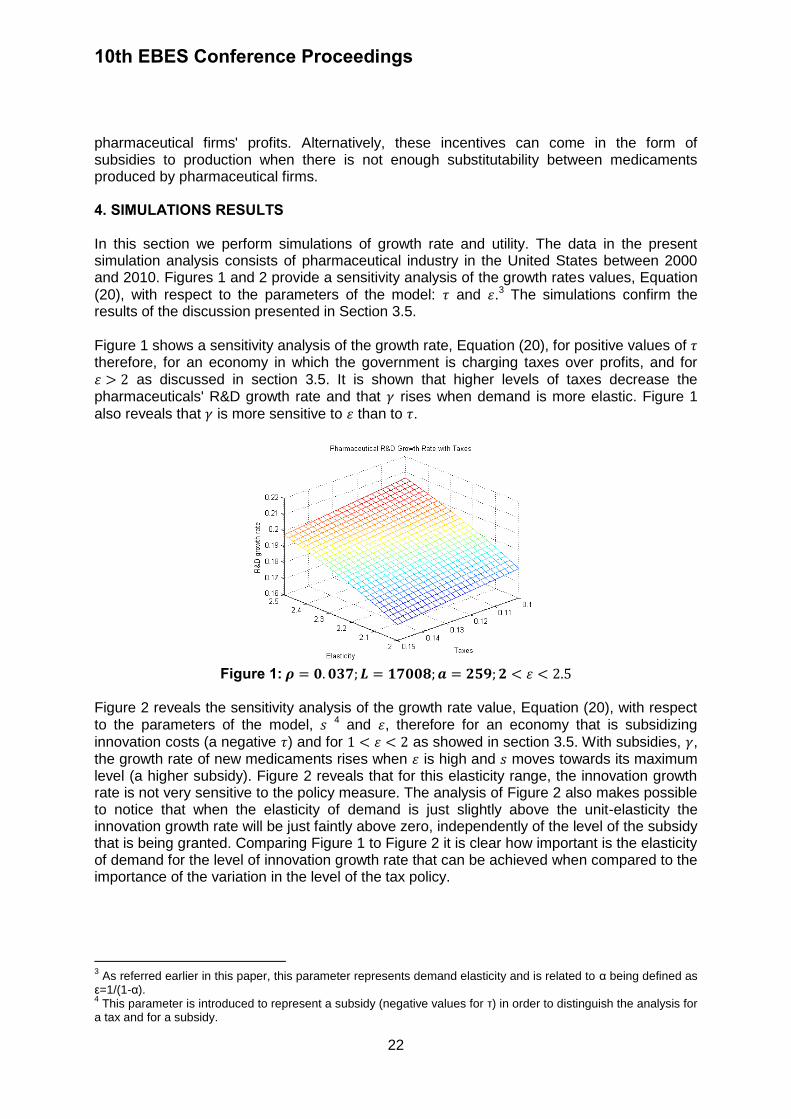
pharmaceutical firms' profits. Alternatively, these incentives can come in the form of subsidies to production when there is not enough substitutability between medicaments produced by pharmaceutical firms. 4. SIMULATIONS RESULTS In this section we perform simulations of growth rate and utility. The data in the present simulation analysis consists of pharmaceutical industry in the United States between 2000 and 2010. Figures 1 and 2 provide a sensitivity analysis of the growth rates values, Equation
(20), with respect to the parameters of the model: and .3 The simulations confirm the results of the discussion presented in Section 3.5. Figure 1 shows a sensitivity analysis of the growth rate, Equation (20), for positive values of therefore, for an economy in which the government is charging taxes over profits, and for as discussed in section 3.5. It is shown that higher levels of taxes decrease the pharmaceuticals' R&D growth rate and that rises when demand is more elastic. Figure 1
also reveals that is more sensitive to than to .
Figure 1:
Figure 2 reveals the sensitivity analysis of the growth rate value, Equation (20), with respect to the parameters of the model, 4 and , therefore for an economy that is subsidizing
innovation costs (a negative ) and for as showed in section 3.5. With subsidies, , the growth rate of new medicaments rises when is high and moves towards its maximum level (a higher subsidy). Figure 2 reveals that for this elasticity range, the innovation growth rate is not very sensitive to the policy measure. The analysis of Figure 2 also makes possible to notice that when the elasticity of demand is just slightly above the unit-elasticity the innovation growth rate will be just faintly above zero, independently of the level of the subsidy that is being granted. Comparing Figure 1 to Figure 2 it is clear how important is the elasticity of demand for the level of innovation growth rate that can be achieved when compared to the importance of the variation in the level of the tax policy.
3 As referred earlier in this paper, this parameter represents demand elasticity and is related to α being defined as
ε=1/(1-α). 4 This parameter is introduced to represent a subsidy (negative values for τ) in order to distinguish the analysis for
a tax and for a subsidy.

10th EBES Conference Proceedings
23
Figure 2:
Figures 3-6 reveal the sensitivity analysis of the utility level, Equation (22), for different
values of the parameters of the model, , and . Figures 3-4 represent the sensitivity analysis of welfare when a tax rate is being charged over pharmaceutical firms' profits and
for , while figures 5-6 represent the sensitivity analysis of welfare when the pharmaceutical firms are receiving a subsidy and for an elasticity range of . 5 Figure 3 respects to the variation in the level of utility when and for increasing tax rates. The results described for the growth rate of innovation, Figure 1, are confirmed with the utility analysis. It is possible to raise taxes and simultaneously obtain higher although decreasing levels of welfare provided there is a high elasticity of demand. The joint evaluation of these two figures also shows that welfare is more sensitive to variations in the tax levels when compared to innovation growth rates.
Figure 3:
The sensitivity analysis of welfare with respect to and is displayed in Figure 4. The utility
level increases when the growth rate of medicaments, , is high and moves towards its minimum level and is considerably more sensitive to the growth rate of innovation than to changes in tax levels.
5 Note that the minimum value for this parameter is related to the minimum value for α.

10th EBES Conference Proceedings
24
Figure 4:
Comparing Figures 3-4 we note that welfare does not depend too strongly on the tax rate,
but it depends on elasticity. Jointly, the figures reveal that for high levels of elasticity ( ), welfare rises with the innovation rate under any value of the tax rate charged over profits. Figure 5 represents variations in the long term level of utility against the parameters of the model, and (a subsidy). The range of variation of elasticity is between 1 and 2, indicating
that as concluded from the analysis of Equation (26). As reported in respect to innovation growth rate from the analysis of Figure 2, changes in welfare are more sensitive to changes in elasticity values than to changes in the tax policy. Nevertheless, the long term level of utility is significantly more sensitive to changes in the level of the subsidy in comparison to the sensitivity of the innovation growth rate, Figure 2. Utility rises as the elasticity increases but the effects over long run utility are decreasing indicating that when a subsidy is being granted there is some satiation of consumers in what refers to variety. Relating the effects of the two alternative tax policies over utility and controlling for different levels of the elasticity of demand, Figures 3 and 5, we note that the long run level of utility is always higher in the presence of a subsidy when compared to taxes and that this result is verified even for the lower levels of elasticity that where considered for the sensitivity analysis of the former tax policy.
Figure 5:
Figure 6 relates rises in welfare to increases in the level of the subsidy, , and in the
innovation growth rate, . The figure reveals that the welfare level is very sensitive to the value of the innovation growth rate but it is not very sensitive to the level of the subsidy. The

10th EBES Conference Proceedings
25
appraisal of Figure 4 and Figure 6 reveals that it is possible to reach higher levels of welfare when there is a subsidy to innovation costs than under a tax over pharmaceutical firms' profits, but the results on the innovation growth rate show that this rate starts from smaller values and is more variable when a subsidy is being granted than when a tax rate is being charged. Additionally, we also notice that welfare is more sensitive to changes in the level of taxes than to changes in the levels of the subsidies.
Figure 6:
Our simulation results confirm our previous analytical results. The elasticity of demand is a determinant feature of the level of innovation growth rate for pharmaceuticals. Higher levels of the growth rate and welfare are possible even in the presence of tax rates over profits, provided this demand elasticity is also high. 5. CONCLUSION In this paper we discuss how the market size for pharmaceuticals' new medicaments can be an important feature of their performance in terms of the innovation growth rate on medicaments. The market size is being represented by the elasticity of demand for pharmaceuticals' new medicaments. This analysis has shown that if the pharmaceutical firms have the proper incentive to innovate they will increase their new medicaments growth rate and consequently expand welfare. In our model, we introduce a government that charges a tax over pharmaceutical firms' profits and reveal that if the elasticity of demand for new medicaments is above 2 it is possible to tax pharmaceutical firms' profits and maintain positive values for their innovation growth rate and therefore increase economy's welfare. Otherwise, for values of the elasticity under 2 it is possible to obtain positive values for the innovation growth rate of new medicaments if the pharmaceutical firms are granted with a subsidy. We have provided an empirical application, based on United States data, to support these results. The results are not very sensitive to changes in the values of the tax policy, especially in the presence of a subsidy, and show a significant response of the growth rate of innovation and welfare to variations in the level of the elasticity of demand. The policy implication is that to improve innovation in the pharmaceutical industry it is important to consider one of two alternatives, either a patent system that reinforces the pharmaceuticals firms wish to innovate and therefore guarantees the diversity that is required by the healthcare sector while taxes are charged over pharmaceutical firms profits, or a
10th EBES Conference Proceedings
26
system based in granting subsidies to innovation and that does not require a high degree of substitutability of medicaments where the supply of new medicaments to the healthcare sector will arise at a smaller pace. Confronting the costs and benefits of either one of these two policies should be the object of further research. REFERENCES Acemoglu, D. and Linn, J., 2004. Market size in innovation: Theory and evidence from the pharmaceutical industry. Quarterly Journal of Economics, 119(3), pp.1049-1090. Bloom, D.E., Boersch-Supan, A., McGee, P. and Seike, A., 2011. Population aging: Facts, challenges, and responses. PGDA Working Paper, 71. Boldrin, M. and Levine, D. K., 2008. Against intellectual monopoly. Cambridge: Cambridge University Press. Busom, I., Corchuelo, M. B. and Martínez-Ros, E., 2012. Tax incentives or subsidies for R&D? UNU-Merit Working Papers, 2012-56. Cerda, R., 2007. Endogenous innovations in the pharmaceutical industry. Journal of Evolutionary Economics, 17(4), pp.473-515. Comanor, W. S. and Scherer, F. M., 2013. Mergers and innovation in the pharmaceutical industry. Journal of Health Economics, 32(1), pp.106-113. Corchuelo, M. B. and Martínez-Ros, E., 2009. The effects of fiscal incentives for R&D in Spain. Technical Report, 09-23, Universidad Carlos III de Madrid. Danzon, P.M., Epstein, A. and Nicholson, S., 2007. Mergers and acquisitions in the pharmaceutical and biotech industries. Managerial and Decision Economics, 28(4-5), pp.307-328. Danzon, P.M. and Keuffel, E.L., 2013. Regulation of the pharmaceutical-biotechnology industry, in economic regulation and its reform: What have we learned? NBER/ University of Chicago Press, Chicago. de Mello-Sampayo, F. and de Sousa-Vale, S., 2012. Financing health care expenditure in the OECD countries: Evidence from a heterogeneous, cross-sectionally dependent panel. ISEG School of Economics and Management Working Paper, WP34/2012/DE, Desmet, K. and Parente, S. L., 2010. Bigger is better: Market size, demand elasticity, and innovation. International Economic Review, 51(2), pp.319-333. Di Masi, J.A., Hansen, R.W. and Grabowski, H.G., 2003. The price of innovation: new estimates of drug development costs. Journal of Health Economics. 22, pp.151-185. Dixit, A.K. and Stiglitz, J. E.,1977. Monopolistic competition and optimum product diversity. The American Economic Review, 67(3), pp.297-308. Dubois, P., de Mouzon, O., Scott-Morton, F., and Seabright, P., 2011. Market size and pharmaceutical innovation. [online] Available at: <http://idei.fr/doc/wp/2011/dmss.pdf> [Accessed 12 June 2013].
10th EBES Conference Proceedings
27
Gambardella, A., Orsenigo, L. and Pammolli, F., 2001. Global competitiveness in pharmaceuticals: A European perspective. Enterprise papers-European Commission, Brussels. Garber, A.M., Jones, C.I., and Romer, P.M., 2006. Insurance and incentives for medical innovation, NBER Working Papers Series, 12080. Grossman, G.M. and Helpman, E., 1991. Innovation and growth in the global economy. Cambridge, MA: Massachusetts Institute of Technology. Hall, B. and Reenen, J.V., 2000. How effective are fiscal incentives for R&D? A review of the evidence. Research Policy, 29(4-5), pp.449-469. Kremer, M., 2002. Pharmaceuticals and the developing world. Journal of Economic Perspectives, 16(4), pp.67-90. Malerba, F. and Orsenigo, L., 2007. Innovation and market structure in the dynamics of the pharmaceutical industry and biotechnology: Towards a history-friendly model. Industrial and Corporate Change, 11(4), pp.667-703. OECD, 2012. Health at a glance: Europe 2012. Paris: OECD Publishing. Rao, A., 2011. Can a R&D tax credit expand investment in product development for global health? Memo, Center for Global Health R&D Policy Assessment. Schumpeter, J., 1942. Capitalism, socialism, and democracy, 5th, 1994 ed, London: Routledge. Toole, A.A., 2012. The impact of public basic research on industrial innovation: Evidence from the pharmaceutical industry. Research Policy, 41(1), pp.1-12. Yin, W., 2008. Market incentives and pharmaceutical innovation. Journal of Health Economics, 27(4), pp.1060-1077.
APPENDIX The simulations relate to the growth rate obtained in Equation (20) and to the utility level obtained in Equation (22). These simulations where performed using data from the United States for the period 2000-2010. The values of the parameters, as well as the ranges used in the simulations of growth rates and the utility level, were drawn from the Organization for Economic Cooperation and Development (OECD database) and can be seen in Table 1. The parameters from the equations of the growth rate and utility are defined as:
: The parameter of elasticity of substitution between any two medicaments, , being
, .
: The discount rate is proxied by the United States "long-term government interest rate", from OECD database, for the period 2000-2010.
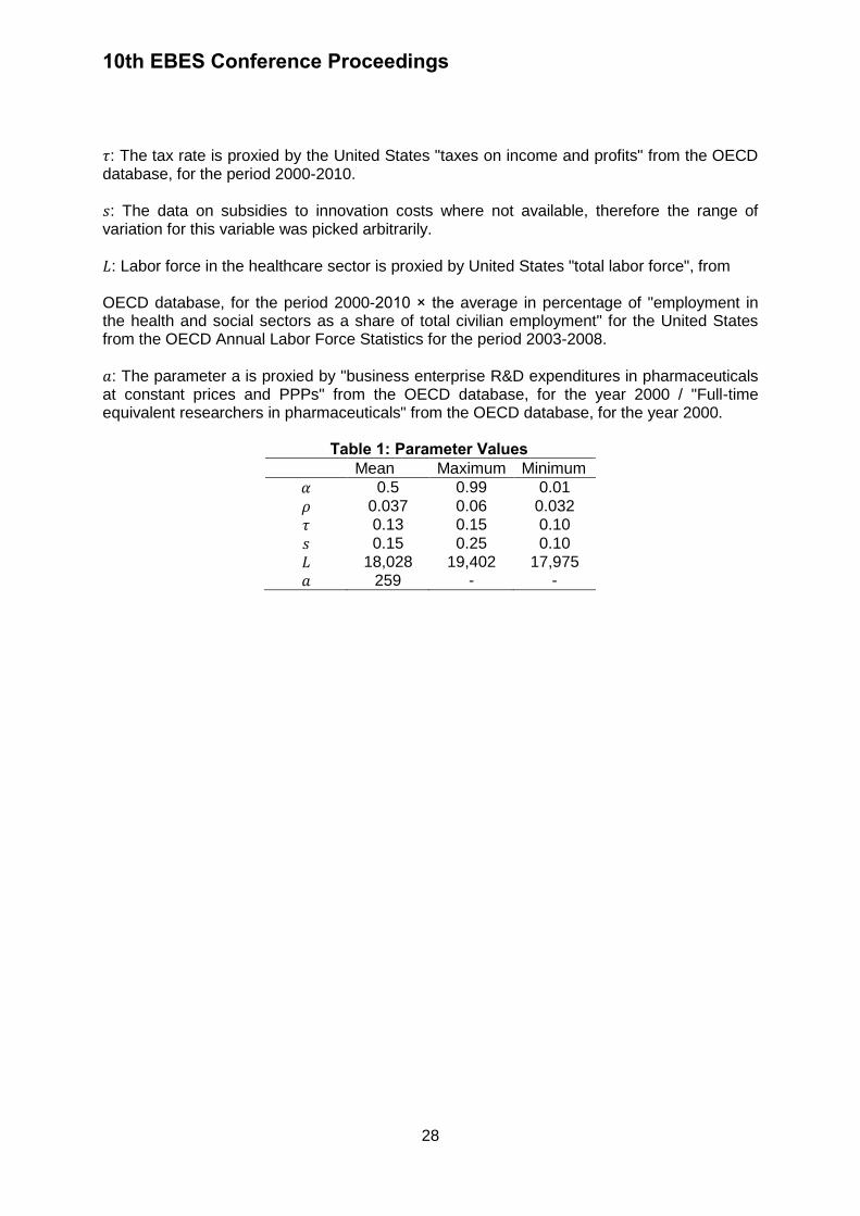
10th EBES Conference Proceedings
28
: The tax rate is proxied by the United States "taxes on income and profits" from the OECD database, for the period 2000-2010. : The data on subsidies to innovation costs where not available, therefore the range of variation for this variable was picked arbitrarily.
: Labor force in the healthcare sector is proxied by United States "total labor force", from OECD database, for the period 2000-2010 × the average in percentage of "employment in the health and social sectors as a share of total civilian employment" for the United States from the OECD Annual Labor Force Statistics for the period 2003-2008. : The parameter a is proxied by "business enterprise R&D expenditures in pharmaceuticals at constant prices and PPPs" from the OECD database, for the year 2000 / "Full-time equivalent researchers in pharmaceuticals" from the OECD database, for the year 2000.
Table 1: Parameter Values Mean Maximum Minimum
0.5 0.99 0.01
0.037 0.06 0.032
0.13 0.15 0.10
0.15 0.25 0.10
18,028 19,402 17,975
259 - -
10th EBES Conference Proceedings 23 - 25 May, 2013. NIPPON HOTEL, ISTANBUL, TURKEY ISBN: 978-605-64002-1-6. WEBSITE: www.ebesweb.org
29
RISK EXPOSURE, RISK-BEARING CAPACITY, AND RISK-COPING STRATEGIES OF URBAN HOUSEHOLDS IN
MALAYSIA
SELAMAH ABDULLAH YUSOF Department of Economics
International Islamic University Malaysia Malaysia
WAN JAMALIAH WAN JUSOH Department of Business Administration International Islamic University Malaysia
Malaysia [email protected]
ROHAIZA ABD ROKIS
Department of Sociology and Anthropology International Islamic University Malaysia
Malaysia [email protected]
Abstract: Household debt in Malaysia has been on an upward trend and increasing at a relatively fast pace. This study provides an in-depth analysis of the current Malaysian urban households’ vulnerabilities and risks and determines differences across the three major ethnic groups of Malay, Chinese and Indian. It examines households’ perception of risk, their capacity to bear risk, and their coping strategies. The study finds that Malaysian urban households are somewhat vulnerable and more so among the Malay households. Households perceive their exposure to small shocks to be somewhat likely, with Malay households’ rating the likelihood to be higher than others. It is found that 6.2% of the households were not able to deal with a small shock, while more than 20% were unable to cope with a large shock. Households will resort to using their savings or cutting down daily expenditure, or turn to family and friends in coping with financial shocks. Malay households have less and fewer sources of funds in meeting unexpected financial needs. Asset poverty among households is high in which 22.9% can survive on basic necessities for only less than three months if their household income is cut-off, and it is more prevalent in Malay households. Keywords: Urban Households, Malaysia, Financial Risk, Capacity-bearing, Coping Strategies, Asset Poverty 1. INTRODUCTION
The 2008-2009 recession was triggered by an unsustainable expansion of the housing sector and subsequent failures in the over-leveraged financial sector, primarily in the United States and Western Europe. A recent IMF research published in the April 2012 World Economic Outlook finds that recessions preceded by larger increases in household debt are more severe. This crisis underscores the importance of household credit market and household financial management in determining the stability of the financial system and the level of
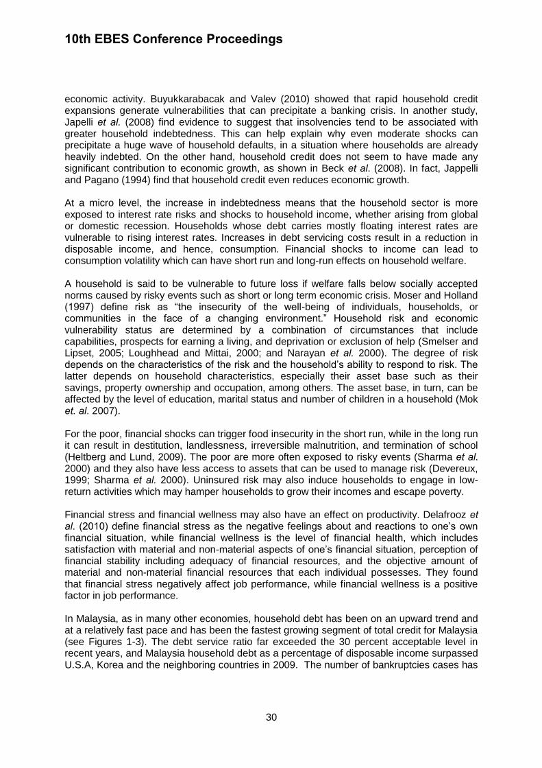
10th EBES Conference Proceedings
30
economic activity. Buyukkarabacak and Valev (2010) showed that rapid household credit expansions generate vulnerabilities that can precipitate a banking crisis. In another study, Japelli et al. (2008) find evidence to suggest that insolvencies tend to be associated with greater household indebtedness. This can help explain why even moderate shocks can precipitate a huge wave of household defaults, in a situation where households are already heavily indebted. On the other hand, household credit does not seem to have made any significant contribution to economic growth, as shown in Beck et al. (2008). In fact, Jappelli and Pagano (1994) find that household credit even reduces economic growth. At a micro level, the increase in indebtedness means that the household sector is more exposed to interest rate risks and shocks to household income, whether arising from global or domestic recession. Households whose debt carries mostly floating interest rates are vulnerable to rising interest rates. Increases in debt servicing costs result in a reduction in disposable income, and hence, consumption. Financial shocks to income can lead to consumption volatility which can have short run and long-run effects on household welfare. A household is said to be vulnerable to future loss if welfare falls below socially accepted norms caused by risky events such as short or long term economic crisis. Moser and Holland (1997) define risk as “the insecurity of the well-being of individuals, households, or communities in the face of a changing environment.” Household risk and economic vulnerability status are determined by a combination of circumstances that include capabilities, prospects for earning a living, and deprivation or exclusion of help (Smelser and Lipset, 2005; Loughhead and Mittai, 2000; and Narayan et al. 2000). The degree of risk depends on the characteristics of the risk and the household’s ability to respond to risk. The latter depends on household characteristics, especially their asset base such as their savings, property ownership and occupation, among others. The asset base, in turn, can be affected by the level of education, marital status and number of children in a household (Mok et. al. 2007). For the poor, financial shocks can trigger food insecurity in the short run, while in the long run it can result in destitution, landlessness, irreversible malnutrition, and termination of school (Heltberg and Lund, 2009). The poor are more often exposed to risky events (Sharma et al. 2000) and they also have less access to assets that can be used to manage risk (Devereux, 1999; Sharma et al. 2000). Uninsured risk may also induce households to engage in low-return activities which may hamper households to grow their incomes and escape poverty. Financial stress and financial wellness may also have an effect on productivity. Delafrooz et al. (2010) define financial stress as the negative feelings about and reactions to one’s own financial situation, while financial wellness is the level of financial health, which includes satisfaction with material and non-material aspects of one’s financial situation, perception of financial stability including adequacy of financial resources, and the objective amount of material and non-material financial resources that each individual possesses. They found that financial stress negatively affect job performance, while financial wellness is a positive factor in job performance. In Malaysia, as in many other economies, household debt has been on an upward trend and at a relatively fast pace and has been the fastest growing segment of total credit for Malaysia (see Figures 1-3). The debt service ratio far exceeded the 30 percent acceptable level in recent years, and Malaysia household debt as a percentage of disposable income surpassed U.S.A, Korea and the neighboring countries in 2009. The number of bankruptcies cases has
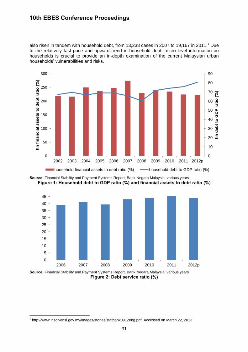
10th EBES Conference Proceedings
31
also risen in tandem with household debt, from 13,238 cases in 2007 to 19,167 in 2011.1 Due to the relatively fast pace and upward trend in household debt, micro level information on households is crucial to provide an in-depth examination of the current Malaysian urban households’ vulnerabilities and risks.
Source: Financial Stability and Payment Systems Report, Bank Negara Malaysia, various years.
Figure 1: Household debt to GDP ratio (%) and financial assets to debt ratio (%)
Source: Financial Stability and Payment Systems Report, Bank Negara Malaysia, various years
Figure 2: Debt service ratio (%)
1 http://www.insolvensi.gov.my/images/stories/statbank0912eng.pdf. Accessed on March 22, 2013.
0
10
20
30
40
50
60
70
80
90
0
50
100
150
200
250
300
2002 2003 2004 2005 2006 2007 2008 2009 2010 2011 2012p
hh d
ebt t
o G
DP
ratio
(%)
hh fi
nanc
ial a
sset
s to
deb
t rat
io (%
)
household financial assets to debt ratio (%) household debt to GDP ratio (%)
0
5
10
15
20
25
30
35
40
45
2006 2007 2008 2009 2010 2011 2012p
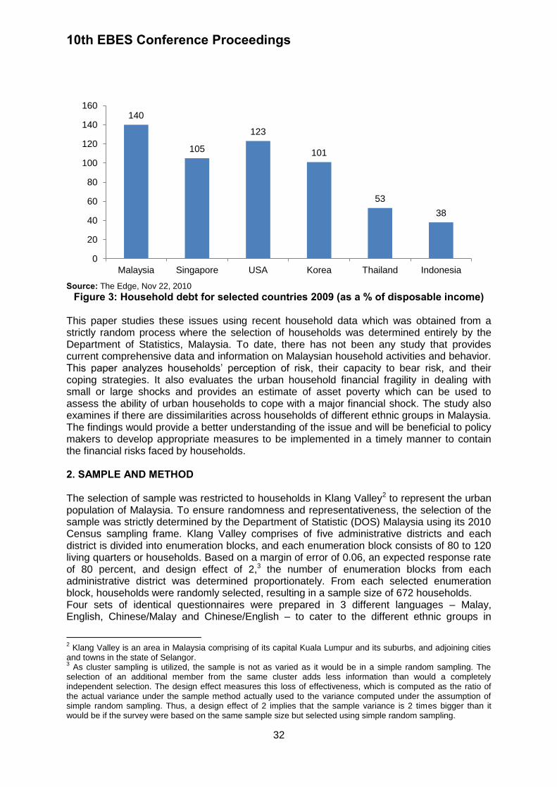
10th EBES Conference Proceedings
32
Source: The Edge, Nov 22, 2010
Figure 3: Household debt for selected countries 2009 (as a % of disposable income)
This paper studies these issues using recent household data which was obtained from a strictly random process where the selection of households was determined entirely by the Department of Statistics, Malaysia. To date, there has not been any study that provides current comprehensive data and information on Malaysian household activities and behavior. This paper analyzes households’ perception of risk, their capacity to bear risk, and their coping strategies. It also evaluates the urban household financial fragility in dealing with small or large shocks and provides an estimate of asset poverty which can be used to assess the ability of urban households to cope with a major financial shock. The study also examines if there are dissimilarities across households of different ethnic groups in Malaysia. The findings would provide a better understanding of the issue and will be beneficial to policy makers to develop appropriate measures to be implemented in a timely manner to contain the financial risks faced by households. 2. SAMPLE AND METHOD
The selection of sample was restricted to households in Klang Valley2 to represent the urban population of Malaysia. To ensure randomness and representativeness, the selection of the sample was strictly determined by the Department of Statistic (DOS) Malaysia using its 2010 Census sampling frame. Klang Valley comprises of five administrative districts and each district is divided into enumeration blocks, and each enumeration block consists of 80 to 120 living quarters or households. Based on a margin of error of 0.06, an expected response rate of 80 percent, and design effect of 2,3 the number of enumeration blocks from each administrative district was determined proportionately. From each selected enumeration block, households were randomly selected, resulting in a sample size of 672 households. Four sets of identical questionnaires were prepared in 3 different languages – Malay, English, Chinese/Malay and Chinese/English – to cater to the different ethnic groups in
2 Klang Valley is an area in Malaysia comprising of its capital Kuala Lumpur and its suburbs, and adjoining cities
and towns in the state of Selangor. 3 As cluster sampling is utilized, the sample is not as varied as it would be in a simple random sampling. The
selection of an additional member from the same cluster adds less information than would a completely independent selection. The design effect measures this loss of effectiveness, which is computed as the ratio of the actual variance under the sample method actually used to the variance computed under the assumption of simple random sampling. Thus, a design effect of 2 implies that the sample variance is 2 times bigger than it would be if the survey were based on the same sample size but selected using simple random sampling.
140
105
123
101
53
38
0
20
40
60
80
100
120
140
160
Malaysia Singapore USA Korea Thailand Indonesia
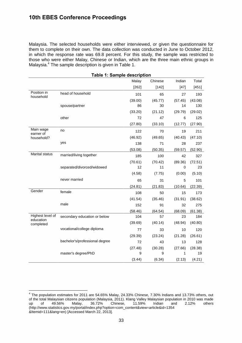
10th EBES Conference Proceedings
33
Malaysia. The selected households were either interviewed, or given the questionnaire for them to complete on their own. The data collection was conducted in June to October 2012, in which the response rate was 69.8 percent. For this study, the sample was restricted to those who were either Malay, Chinese or Indian, which are the three main ethnic groups in Malaysia.4 The sample description is given in Table 1.
Table 1: Sample description Malay Chinese Indian Total
[262] [142] [47] [451]
Position in household
head of household 101 65 27 193
(39.00) (45.77) (57.45) (43.08)
spouse/partner 86 30 14 130
(33.20) (21.12) (29.79) (29.02)
other 72 47 6 125
(27.80) (33.10) (12.77) (27.90)
Main wage earner of household?
no 122 70 19 211
(46.92) (49.65) (40.43) (47.10)
yes 138 71 28 237
(53.08) (50.35) (59.57) (52.90)
Marital status married/living together 185 100 42 327
(70.61) (70.42) (89.36) (72.51)
separated/divorced/widowed 12 11 0 23
(4.58) (7.75) (0.00) (5.10)
never married 65 31 5 101
(24.81) (21.83) (10.64) (22.39)
Gender female 108 50 15 173
(41.54) (35.46) (31.91) (38.62)
male 152 91 32 275
(58.46) (64.54) (68.09) (61.38)
Highest level of education completed
secondary education or below 104 57 23 184
(39.69) (40.14) (48.94) (40.80)
vocational/college diploma 77 33 10 120
(29.39) (23.24) (21.28) (26.61)
bachelor's/professional degree 72 43 13 128
(27.48) (30.28) (27.66) (28.38)
master's degree/PhD 9 9 1 19
(3.44) (6.34) (2.13) (4.21)
4 The population estimates for 2011 are 54.65% Malay, 24.33% Chinese, 7.30% Indians and 13.73% others, out
of the total Malaysian citizens population (Malaysia, 2011). Klang Valley Malaysian population in 2010 was made up of 49.56% Malay, 36.72% Chinese, 11.59% Indian and 2.12% others (http://www.statistics.gov.my/portal/index.php?option=com_content&view=article&id=1354 &Itemid=111&lang=en) [Accessed March 22, 2013].
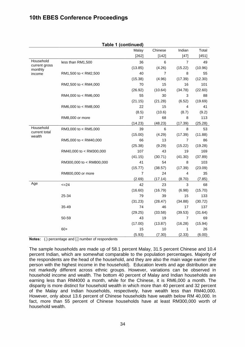
10th EBES Conference Proceedings
34
Table 1 (continued)
Malay Chinese Indian Total
[262] [142] [47] [451]
Household current gross monthly income
less than RM1,500 36 6 7 49
(13.85) (4.26) (15.22) (10.96)
RM1,500 to < RM2,500 40 7 8 55
(15.38) (4.96) (17.39) (12.30)
RM2,500 to < RM4,000 70 15 16 101
(26.92) (10.64) (34.78) (22.60)
RM4,000 to < RM6,000 55 30 3 88
(21.15) (21.28) (6.52) (19.69)
RM6,000 to < RM8,000 22 15 4 41
(8.5) (10.6) (8.7) (9.2)
RM8,000 or more 37 68 8 113
(14.23) (48.23) (17.39) (25.28)
Household current total wealth
RM3,000 to < RM5,000 39 6 8 53
(15.00) (4.29) (17.39) (11.88)
RM5,000 to < RM40,000 66 13 7 86
(25.38) (9.29) (15.22) (19.28)
RM40,000 to < RM300,000 107 43 19 169
(41.15) (30.71) (41.30) (37.89)
RM300,000 to < RM800,000 41 54 8 103
(15.77) (38.57) (17.39) (23.09)
RM800,000 or more 7 24 4 35
(2.69) (17.14) (8.70) (7.85)
Age <=24 42 23 3 68
(16.60) (16.79) (6.98) (15.70)
25-34 79 39 15 133
(31.23) (28.47) (34.88) (30.72)
35-49 74 46 17 137
(29.25) (33.58) (39.53) (31.64)
50-59 43 19 7 69
(17.00) (13.87) (16.28) (15.94)
60+ 15 10 1 26
(5.93) (7.30) (2.33) (6.00)
Notes: (.) percentage and [.] number of respondents
The sample households are made up of 58.1 percent Malay, 31.5 percent Chinese and 10.4 percent Indian, which are somewhat comparable to the population percentages. Majority of the respondents are the head of the household, and they are also the main wage earner (the person with the highest income in the household). Education levels and age distribution are not markedly different across ethnic groups. However, variations can be observed in household income and wealth. The bottom 40 percent of Malay and Indian households are earning less than RM4000 a month, while for the Chinese, it is RM6,000 a month. The disparity is more distinct for household wealth in which more than 40 percent and 32 percent of the Malay and Indian households, respectively, have wealth less than RM40,000. However, only about 13.6 percent of Chinese households have wealth below RM 40,000. In fact, more than 55 percent of Chinese households have at least RM300,000 worth of household wealth.
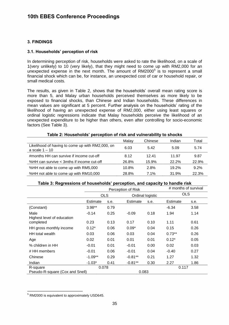
10th EBES Conference Proceedings
35
3. FINDINGS 3.1. Households’ perception of risk
In determining perception of risk, households were asked to rate the likelihood, on a scale of 1(very unlikely) to 10 (very likely), that they might need to come up with RM2,000 for an unexpected expense in the next month. The amount of RM20005 is to represent a small financial shock which can be, for instance, an unexpected cost of car or household repair, or small medical costs. The results, as given in Table 2, shows that the households’ overall mean rating score is more than 5, and Malay urban households perceived themselves as more likely to be exposed to financial shocks, than Chinese and Indian households. These differences in mean values are significant at 5 percent. Further analysis on the households’ rating of the likelihood of having an unexpected expense of RM2,000, either using least squares or ordinal logistic regressions indicate that Malay households perceive the likelihood of an unexpected expenditure to be higher than others, even after controlling for socio-economic factors (See Table 3).
Table 2: Households’ perception of risk and vulnerability to shocks
Malay Chinese Indian Total
Likelihood of having to come up with RM2,000, on a scale 1 – 10
6.03 5.42 5.09 5.74
#months HH can survive if income cut-off 8.12 12.41 11.97 9.87
%HH can survive < 3mths if income cut-off 26.8% 15.9% 22.2% 22.9%
%HH not able to come up with RM5,000 10.8% 2.8% 19.2% 9.2%
%HH not able to come up with RM10,000 28.8% 7.1% 31.9% 22.3%
Table 3: Regressions of households’ perception, and capacity to handle risk
Perception of Risk # months of survival
OLS Ordinal logistic OLS
Estimate s.e. Estimate s.e. Estimate s.e.
(Constant) 3.98** 0.79
-6.34 3.58
Male -0.14 0.25 -0.09 0.18 1.94 1.14 Highest level of education completed 0.23 0.13 0.17 0.10 1.11 0.61
HH gross monthly income 0.12* 0.06 0.09* 0.04 0.15 0.26
HH total wealth 0.03 0.06 0.03 0.04 0.73** 0.26
Age 0.02 0.01 0.01 0.01 0.12* 0.05
% children in HH -0.01 0.01 -0.01 0.00 0.02 0.03
# HH members -0.01 0.06 -0.01 0.04 -0.40 0.27
Chinese -1.09** 0.29 -0.81** 0.21 1.27 1.32
Indian -1.03* 0.41 -0.81** 0.30 2.27 1.86
R-square Pseudo-R-square (Cox and Snell)
0.078 0.083
0.117
5 RM2000 is equivalent to approximately USD645.

10th EBES Conference Proceedings
36
3.2. Household vulnerability to shocks: capacity to handle risk
For the measurement of vulnerability of households to shocks, the research focuses on two aspects. Firstly, the households were asked how long they will be able to survive with their basic needs if their income is suddenly cut-off. Secondly, households were asked how confident they were of coming up with RM2,000 for an unexpected expense on their own.6 Households were also asked if they are able to come up with RM5000 and RM10,000,7 respectively, from any source at all if an unexpected need arises within the next month. These amounts are chosen to represent medium and large financial shocks. The results, as presented in Table 2, show that Malay households are the most vulnerable, in which the average number of months they can survived with basic necessities if their income is cut-off is 8.12 months. This is significantly much lower than that of Chinese households (at 1 percent level) and Indian households (at 5 percent level), which are 12.41 and 11.97 months, respectively. There is no significant difference between Chinese and Indian households. Additionally, Malay households have the highest level of asset poverty, with more than a quarter of the households can only survive on basic necessities for less than 3 months.8 The percentages are lower for Indian households (22.2%), and much lower for Chinese households (15.9%). Regression results, as shown in Table 3, indicate that the differences are due to the different levels of wealth of the households. Controlling for this factor, and other socio-economics variables, there are no significant differences across ethnic groups. About 10.8 percent of Malay households are not able to raise RM5,000 from any source if they were to face with this unexpected expense, and 28.8 percent of them will not able to do so if the amount is RM10,000. Indian households are in a worse position, with about 19.2 percent, and 31.9 percent not able to obtain RM5000, and RM10,000 from any source. Chinese households, on the other hand, are in a more comfortable situation in which more than 92 percent of them are able to raise RM10,000 from some source. With regards to small risks, 6.2% of the households were not able to endure a small financial shock as they were certain that they could not raise RM2000 if the unexpected need arises.
3.3. Household vulnerability to shocks: Coping strategies
Table 4 summarizes the findings on the various sources used by households to raise the fund needed for unexpected financial expenses. Thirteen sources of funds were listed9 and these sources were grouped into six main options: (i) saving; (ii) social networks; (iii) traditional credit; (iv) alternative credit; (v) work more; and (vi) sell possessions. Households will resort to using their own savings or cutting down daily expenditure, or turn to family and friends in coping with financial shocks. The study finds variation across households of different ethnicity. Compared to Chinese households, the Malays are more
6 The response options to the question are: (i) I am certain I could come up with the RM2,000; (ii) I could probably
come up with the RM2,000; (iii) I could probably not able to come up with the RM,2000; and (iv) I am certain I could not raise the RM2000. 7 RM5,000 is approximate USD1600 and RM10,000 is about USD3,215.
8 This is a measure of asset poverty, in which a household is not able to survive on basic necessities for at least 3
months if the household income is cut-off. 9 The sources are: (i) use savings; (ii) borrow or ask help from family; (iii) borrow or ask help from friends; (iv)
borrow from unlicensed money lender/loan shark; (v) take out a personal loan from a bank/financial institution; (vi) use credit cards; (vii) liquidate or sell investments; (viii) work overtime, get a second job, or another member of household would work longer or go to work; (ix) pawn as asset; (x) sell things I owned, except home; (xi) sell home; (xii) cut down on daily expenses; and (xiii) other.

10th EBES Conference Proceedings
37
likely to rely on alternative credit, either by pawning their assets or borrow from loan shark to cover unexpected small financial expenses. Malay households also will resort to working more to get the funds for any level of unexpected expenditures. In addition, they are less likely to rely on family and friends to deal with large financial shocks. Malay households rely on relatively more sources to obtain funds for small financial shocks, but utilize fewer sources for large shocks. This finding indicates that Malay households do not have enough of their own funds and have to use several other sources to meet even small shocks. For a large shock, they have fewer sources, and less funds in meeting these unexpected financial needs.
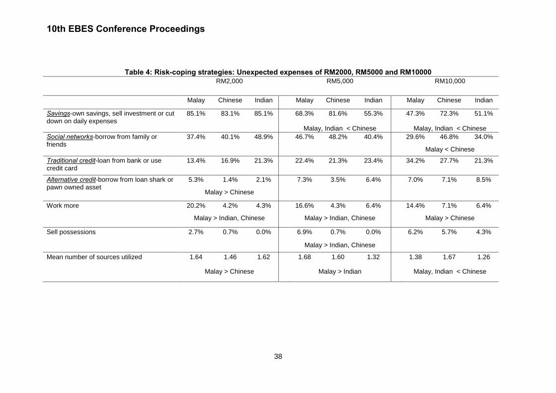
10th EBES Conference Proceedings
38
Table 4: Risk-coping strategies: Unexpected expenses of RM2000, RM5000 and RM10000 RM2,000 RM5,000 RM10,000
Malay Chinese Indian Malay Chinese Indian Malay Chinese Indian
Savings-own savings, sell investment or cut down on daily expenses
85.1% 83.1% 85.1% 68.3% 81.6% 55.3% 47.3% 72.3% 51.1%
Malay, Indian < Chinese Malay, Indian < Chinese
Social networks-borrow from family or friends
37.4% 40.1% 48.9% 46.7% 48.2% 40.4% 29.6% 46.8% 34.0%
Malay < Chinese
Traditional credit-loan from bank or use credit card
13.4% 16.9% 21.3% 22.4% 21.3% 23.4% 34.2% 27.7% 21.3%
Alternative credit-borrow from loan shark or pawn owned asset
5.3% 1.4% 2.1% 7.3% 3.5% 6.4% 7.0% 7.1% 8.5%
Malay > Chinese
Work more 20.2% 4.2% 4.3% 16.6% 4.3% 6.4% 14.4% 7.1% 6.4%
Malay > Indian, Chinese Malay > Indian, Chinese Malay > Chinese
Sell possessions 2.7% 0.7% 0.0% 6.9% 0.7% 0.0% 6.2% 5.7% 4.3%
Malay > Indian, Chinese
Mean number of sources utilized 1.64 1.46 1.62 1.68 1.60 1.32 1.38 1.67 1.26
Malay > Chinese Malay > Indian Malay, Indian < Chinese
10th EBES Conference Proceedings
39
4. DISCUSSION AND CONCLUSION This study uses recent household data which was obtained from a strictly random process to examine the vulnerability of Malaysian households in facing financial shocks and their capacity to bear the risk. The results indicate Malay households, which form the majority of the urban population, are the most vulnerable and have lower risk-bearing capacities. Although they perceive the likelihood of facing financial shocks to be higher than others, are less able to cope with a major financial shock compared to Chinese and to a certain extent, Indian households. The higher levels of vulnerability in Malay households can be attributed to them having lower levels of wealth, making them more exposed to any form of financial shock, whether small or large. It is of concern when more than a quarter of the Malay households cannot survive at least three months if their income is cut-off. Additionally, not only are they not having their own funds, they have fewer sources to obtain these funds when faced with a relatively large financial shock. In order to mitigate this phenomenon, programs must be designed to assist households to manage their income, to save and invest to protect themselves against any form of risk. These programs must effectively improve households’ financial capability and capacity, and they have to be structured in ways that take into account the different levels of wealth, attitudes, aptitudes and ethnic backgrounds. Free consultation regarding financial products available in the market and making wise financial investment should be provided to low-income households. Household debt must be constantly monitored to ensure that it is sustainable, and safety measures must be put in place to protect households and the economy when faced with a crisis, either globally or locally. REFERENCES Beck, T., Buyukkarabacak, B., Rioja, F., and Valev, N., 2008. Who gets the credit? Household vs. firm lending across countries. World Bank Policy Research Working Paper 4661. Buyukkarabacak, B. and Valev, N., 2010. The role of household and business credit in banking crises. Journal of Banking and Finance, 34(6), pp.1247-1256. Devereux, S., 1999. Making less last longer: Informal safety nets in Malawi. IDS Discussion Paper, 373. Heltberg, R. and Lund, N., 2009. Shocks, coping, and outcomes for Pakistan’s poor: Health risks predominate. Journal of Development Studies, 45(6), pp.889-910. Japelli, T., Pagano, M., and di Maggio, M., 2008. Household indebtedness and financial fragility. Centre for Studies in Economics and Finance Working Paper, 208. Loughhead, S. and Mittai, O., 2000. Urban poverty and risk in India: A social perspective. Paper presented at the Urban Forum: Urban Poverty Reduction in the 21st Century, sponsored by the World Bank, April 3-5, 2000. Chantilly, Virginia. Malaysia, 2011. Population distribution by local authority areas and Mukims, 2010 [online] Available at:

10th EBES Conference Proceedings
40
<http://www.statistics.gov.my/portal/index.php?option=com_content&view=article&id=1354&Itemid=111&lang=en> [Accessed March 28, 2013]
Mok, T.Y., Gan C., and Sanyal, A., 2007. The determinants of urban household poverty in Malaysia. Journal of Social Sciences, 3(4), pp.190-196. Moser, C. and Holland, J., 1997. Household responses to poverty and risk: Confronting crisis in Cawama, Lusaka, Zambia. Urban Management Programme, Report No.24. The World Bank: Washington, D.C. Narayan, D., Patel, R., and Schafft, K., Rademacher, A., and Koch-Schulte, S., 2000. Voices of the poor: Can anyone hear us? New York: Oxford University Press. Sharma, M., Burton, I., van Aalst, M., Dilley, M., and Acharya, G., 2000. Reducing vulnerability to Environmental variability: Background paper to the World Bank’s environmental strategy. Washington, D.C.: The World Bank. Smelser, N.J. and Lipset M.S., 2005. Social structure and mobility in economic development. US: Aldine Transaction.
10th EBES Conference Proceedings 23 - 25 May, 2013. NIPPON HOTEL, ISTANBUL, TURKEY ISBN: 978-605-64002-1-6. WEBSITE: www.ebesweb.org
41
A REVIEW OF IMPACT MAKING TECHNOLOGIES IN SUPPLY CHAIN MANAGEMENT
ARIFUSALAM SHAIKH
College of Business Administration Prince Mohammad Bin Fahd University
Saudi Arabia [email protected]
MOHAMMAD KHALIFA AL-DOSSARY
College of Business Administration Prince Mohammad Bin Fahd University
Saudi Arabia [email protected]
Abstract: An efficient supply chain management embedded with latest technology is the key for the success of any global organization. While the efficiency of the managers throughout the supply chain is not to be under estimated, it has been proved time and again that those managers who adopt or even create technology to enhance their supply chain operations have achieved outstanding results. The invention of internet and following IT technologies has been the foundation for the evolution of supply chain management. The aim of this study is to review major technologies that emerged to facilitate supply chain management. Among some of the significant technologies that retailers around the globe use for their business processes are Enterprise Resource Planning (ERP), Warehouse Management System (WMS), Transportation Management System (TMS) and Automatic Identification and Data Collection (AIDC). Some customer based technologies in use are Vendor-Managed Inventory (VMI), Point of Sale (POS) and Collaborative Planning, Forecasting and Replenishment (CPFR), etc. The recent developments in RFID technologies have opened doors for major applications in the field of SCM. This paper will consider few impact making technologies and discuss their applications, benefits and how they sustained the challenges of SCM. Keywords: Supply Chain Management, Technology, Supply Chain Efficiency 1. INTRODUCTION In simple words supply chain management (SCM) can be defined as the “combination of art and science that goes into improving the way your company finds the raw components it needs to make a product or service and deliver it to customers” (Waligum, 2008). A leading association of operations management, APICS in its dictionary defines SCM as the “design, planning, execution, control, and monitoring of supply chain activities with the objective of creating net value, building a competitive infrastructure, leveraging worldwide logistics, synchronizing supply with demand and measuring performance globally”. The latter definition includes crucial elements that are engraved with the success of supply chain such as competitive infrastructure and logistics. This elaborated definition signifies the need of using existing or developing new technology to build an efficient supply chain. SCM stages spans through the supplier’s supplier, direct suppliers, manufacturers, distributors, retailers and customers. Between these stages the movement and storage of raw materials, work-in-process inventory, and finished goods from point of origin to point of consumption is handled through a coordinated effort from all parties. It is obvious that the
10th EBES Conference Proceedings
42
success of any supply chain thus relies on the efficiency at the operational levels of each stage as well as thorough coordination in terms of sharing information. Such a need of high-level coordination invites the use of sophisticated technologies to make peerless integration of process and data exchange. The emergence of globalization has created international businesses that operate all over the world increasing the physical distance between the various stages of supply chain. On the other hand, it also opened markets for new vendors and new markets that are the terminal anchors of any supply chain. E-commerce plays a vital role in keeping these terminals intact by allowing the organization to exchange crucial data in a time efficient manner, which significantly reduces the processing times between different stages. However, it is quite challenging to make the data exchange between different stages efficient including optimizing upstream and downstream logistics. Several technologies thus evolved and many gave birth to newer technologies to cater the challenges that emerged in the quest of making the supply chain efficient and responsive. The objective of SCM is to maximize the overall value added and is measured as supply chain surplus, defined as the difference between the customer value and the supply chain cost (Chopra and Meindl, 2007). Pore (2012) proposed six ultimate objectives of supply chain that included factors other than maximizing overall value generated. The other objectives are to find foundations for revenue and cost, refill of materials or products when needed, optimizing cost quality, improving response time to shorten time to order and finding a better way to reach market faster. The accomplishment of these objectives can only be enhanced by using the right technology in the right place. The purpose of this paper is two folds, one to review the technologies that had an impact on SCM and discuss the key features that sustained the challenges of SCM and the other is to address the challenges of emerging technologies that facilitate achieving the major objectives of SCM. The paper will cover fundamental concepts in SCM including the supply-chain objective, the ideology of supply-chain components, the three flows, and the cycles involved in supply-chain in section 2. Section 3 will present the technologies used in coordinating the supply-chain from macro processes point of view which involves supplier relationship management, customer relationship management, and internal supply chain management. A literature review of the technologies utilized by SCM is then presented in section4. In section 5, selected technologies will be discussed that had an impact on the SCM and sustained the challenges evolved with the growing demands of the organizations. Summary and future recommendation will be provided in section 6. 2. SUPPLY CHAIN MANAGEMENT IN BRIEF To understand the challenges of SCM it is now imperative to study the major components of SCM which shape supply-chain stages, namely; supplier, manufacturer, distributor, retailer and consumer. Supply-chain components are planning, sourcing, making, delivering, and returning. As per Rouse (2010), there are three flows in supply chain management. They are product flow, information flow, and funds (or financing) flow. A good management of those flows triggers the success of the supply-chain for the reason that each has its importance in enhancing profitability and overall productivity. The product flow embrace the set of actions that handle products and service transportation from suppliers to customers, as well as any reverse movement of goods and services. The information flow includes conveying orders to consumers and updating the condition of the transmission. The funds flow is composed of credit terms, imbursement scheduling, and shipment and designation ownership. Later on,

10th EBES Conference Proceedings
43
those flows will be mentioned intentionally or unintentionally through the paper, as it is obvious that they need to be managed by a technology. 3. SUPPLY-CHAIN TECHNOLOGICAL MACRO PROCESSES Technology plays a crucial role in all aspects of SCM ranging from the supply-chain objectives, supply-chain components and flows, and ending up with supply-chain stages and cycles. A clear picture can be obtained by understanding the three main macro processes that aid in classifying the technological aspects of supply-chain management. As per to Chopra and Meindl (2007), technology macro processes of SCM are Supplier Relationship Management, Customer Relationship Management, and Internal Supply-Chain Management. An excellent coordination between these processes may lead to excellence in overall supply-chain performance. In addition, to coordinate among these macro processes, major organizations use Enterprise Resource Planning (ERP) systems (will be discussed later in Section 5.1). Some of the popular ERP systems used by large organizations are SAP, Oracle, PeopleSoft, JD Edwards, and Baan. 3.1. Supplier relationship management Abbreviated as SRM, it is the regulation in tactically setting up, and controlling, every interaction that occur with a third party company that supply products and services to another firm to maximize the end result of those deals. The primary goal of SRM is to rationalize and produce value out of the processes between a company and its suppliers. SRM is a platform that initiates closer, more cohesive relationships among vital suppliers to explore and recognize new value and reduce risk. Use of appropriate SRM software can thus facilitate effective communication between a firm and its suppliers and utilize diverse business practices and terminology leading to lower manufacturing costs and higher quality. Manugistics, PeopleSoft, SAP, and many other software companies provide SRM solutions. With the latest technologies, coordination with suppliers is made more easy and smooth than before. Good SRM software provides solution to issues related to obtaining goods and services, controlling inventory, and handling materials. The major tasks accomplished among others are design collaboration, sourcing, negotiating, purchasing and supply collaboration. 3.2. Customer relationship management Abbreviated as CRM, it includes a firm’s interactions with consumers, and clients. Using technology in CRM enables automation, organization, and synchronization of business processes that facilitates sales activities, along with marketing and customer services. Since customers of big organizations are usually in vast numbers, it is inevitable to use automated software to communicate with customers to cater their needs. For example, Amazon.com with the most huge respiratory of customers developed and customized a system that enabled them to send emails to each customer with the customized promotions. They also use RFID tags to track information from their customers (discussed in details in section 5.2). Some of the common tasks that are done in CRM include marketing, selling, order management and call/service center. 3.3. Internal supply chain management In SRM and CRM, we covered the macro processes with external interactions that involve greater risk. However, Internal Supply Chain Management (ISCM) is also crucial and is
10th EBES Conference Proceedings
44
concerned with internal operations or any organization. It involves all tasks related to planning, and gratifying a consumer order. With the help of right tools, ISCM can provide important and related information easily accessible, efficient inventory management, and efficient utilization of funds. The regular tasks ISCM among others include strategic planning, demand planning, supply planning, fulfillment and field service. 4. REVIEW OF TECHNOLOGIES A trend analysis is now presented to determine the observations of various researchers about the technologies supporting supply-chain management. The period of study is focused from year 2001 to 2012 as this was the prime period when the technologies started to play a major role and ever since are continuously evolving to integrate supply chain process. Kumar (2001) highlighted some facts about emerging technologies. He observed that any manager did not want a product or service to be just delivered to the destined consignee. Rather he/she wants to make sure that a product is installed properly, consumer is educated about the product usage, product is maintained and repaired when needed, and customers made the most value out of the offered product and rendered service. To ensure all that, Kumar hinted to use the emerging technologies that included Enterprise Resource Planning (ERP), and the advanced version of it, the extended ERP. Kumar believed that ERP systems, executive information systems, and decision support systems, will be key players to achieve cost efficiencies and organizational effectiveness. Above that, he also emphasized the use of Advanced Planning Systems (APS). However, in the modern days, APS is integrated as part of the ERP systems. We will depart from year 2001 and hoop down into year 2003 where Singh (2003) had different observations. Singh was allocating a great portion of attention towards the development of software, optimization, constraint programming, and artificial intelligence. The observations of Singh were based on supply-chain managers’ ideas to transfer information and raw data into information and knowledge that can be used for operations. He further added that various forms of supply chain management applications are among the enabling technologies transforming how business markets operate. Singh highlighted about the emerging Automatic Data Capture (ADC) that is capable of handling bar code scanning, voice recognition, and radio frequency data capture (RFDC). However, RFID was then considered the most pumping technology. The only fact that stopped the use of RFID at that time was its high cost. Singh also led the attention towards another important budding technology for the supply-chain field, which is Artificial Intelligence (AI). Singh confirmed that AI techniques have been put to use in multiple segments of the supply chain and has its critical benefit in affording the best basis for solving complex supply-chain problems. AI does that by neural networking, clustering, and classification techniques that enable the AI to offer intelligent decision-making data and online analytical processing. Companies such as IBM, Congos, SAS, Oracle, and SPSS can implant the AI as per Singh. Leaving year 2003 to move ahead and examine what was grasping distinct researchers’ attention in the consecutive years 2005 and 2006. Massive numbers of authors were jotting down all their thoughts and researches about the Radio Frequency Identification (RFID) technology. In year 2005, Angeles mentioned that RFID had the potential of closing some of the information gaps in the supply chain, especially in retailing and logistics, and further added that, as a mobile technology, RFID can enable ‘process freedoms’ and real-time visibility into supply chains. We can observe how RFID was seen as supply-chain’s most
10th EBES Conference Proceedings
45
advanced technology. Loebbecke (2005) also stated that RFID has gained enormous attention in various industry sectors, the media, and in academic research. Loebbecke confirmed what Angeles and others mentioned about RFID’s huge surge trend lately. As a matter of fact, Loebbecke emphasized on RFID application on retailer, while Angeles was determined to cover RFID as of retailing and logistics and still RFID has its importance in different operational areas in supply-chain. RFID sustained its significance and remained the talk of the year in year 2006. Wamba et al (2006) concluded that RFID and EPC (Electronic Product Code) were the enablers to provide intelligent B2B e-Commerce supply chain management. From those sources, we can assure that RFID can give elucidation to many problems in the supply chain. After years 2005 and 2006, we now advance to cover the following successive years 2007, 2008, and 2009. Harrington (2007) gathered the most promising technologies in supply-chain. She mentioned five, which were RFID, multi-enterprise visibility systems, people enabling software, execution-driven planning solutions, and human supply chain technology. From different reports, it seems obvious that RFID has maintained itself as the most essential technology; yet, the focus is more on RFID’s problems and challenges. Viehland and Wong (2007) found number of issues that have to be resolved in terms of RFID's future and implementation. Failure to address these issues could result in failure of an RFID implementation, which results in a waste of significant resources and potential loss of strategic opportunities. Additional the same year, Niederman et al (2007) had the same understanding of RFID issues and stated that the key issue in implementing such a system will be developing appropriate business rules, particularly for handling new exceptions that arise from having the increased amount of data generated from RFID implementations. They also observed that of RFID could serve various types of applications that include retailing (Wal-Mart), and politics (U.S. Department of Defense). Year 2008 and 2009 had new emphasis on RFID. Anne et al (2008) were concerned about a very important concept in technology that is advancing rapidly in regards to supply-chain, which is self-organized Supply-Chain Networks (SCN). According to them SCNs are offering an alternative as they enjoy the flexibility needed to respond in real time. Furthermore, a collaborative research project was conducted from Auckland University in year 2008 that examined the technologies that will be emerging for the future for supply-chain. The research presented by Soon (2008) focused on the oil industry and short listed four very rapid up-and-coming technologies which are RFID, GPS (Global Positioning Systems), AIDC (Automatic Identification and Data Capture), and OCR (Optical Character Recognition). As year 2009 arrived, writers wanted to get out of the regular domain of RFID and concentrate on different frameworks in RFID functionality. De Virgilio et al (2008) demanded a new structure towards the concept of incremental aggregation of RFID data that has a significant impact in strategic decision-making and hence, enhance overall supply-chain performance. Further, Dai (2009) introduced the new concept of cloud computing as in information technology which can play a vital role in supply chain management. He adhered to relate it to small and medium sized businesses of supply-chain management and how it can help in developing virtual information systems. Year 2009 had another look from Xie (2009) where he made a study on retailers and the emerging technologies and he listed his top four, which are RFID, EDI, POS (Point of Sales), and DM (Data Mining). Lately, the booming talk remains mostly on two vital topics regarding technology in supply-chain. It roams around RFID, again, and the hot topic of e-government and its affect when integrating it to a supply-chain business. Year 2010 shed the light on RFID through Mo and
10th EBES Conference Proceedings
46
Lorchirachoonkul (2010) where they had a new idea that was to develop an easy channel for third party service providers to stay in touch with their customers and suppliers. Other than that, Chen et al (2011) had their insight to use the SCN with the e-government ideology. This was to end all the government needed documentation and approvals in easier manner which reduces cost and enhance responsiveness time. 5. EMERGING TECHNOLOGIES IN SUPPLY-CHAIN MANAGEMENT As seen in the previous section, several technologies evolved to assist coordination of activities in supply chain, and there were a selected few who actually made an impact overall on the way of performing business in global market. Among all those technologies, it can be concluded that two of them made a major impact and sustained the challenges of supply chain coordination in growing international business, which are ERP systems and RFID technology. These technologies and their characteristics will now be discussed. 5.1. ERP systems The Enterprise Resource Planning system (ERP) integrates internal and external management information of a whole organization, containing finance/accounting, manufacturing, sales and services, customer relationship management (CRM), etc. The ERP systems are automated via software applications such as SAP system, Oracle, and peopleSoft. The system works on controlling the workflow of business processes across an organization to avoid duplication of data. Supply-chain management can be optimized by using ERP systems. Let us take an example to comprehend it. In Saudi Aramco, they deal with thousands of suppliers on daily basis for procuring small and large commodities. With the use of their powerful SAP system (an ERP system), they do not have to contact each supplier personally to share the forecasts, orders, and other information needed by a supplier. Ideally, the system will automate those types of processes and will make it consistent amongst the whole supply-chain. Information flow and product flow along all supply-chain stages will be recognized by all stages as required. It is clear that there is an excessive need to have visible customer demand that is up-to-date. Suppliers need demand information and feedback from customer to prepare commodities to be supplied. Manufacturers need information of supply chain inventories, manufacturing planning, scheduling, and collect customer demographics. Distributors and retailers need information about deadlines of handing finished goods, customer demand from different regional areas, and inventory levels. Finally, customers need information concerning quality of product or service, dates of releasing those products, and post information used for retaining and maintenance purposes. From all stages, we can see how it is vital to have a platform as ERP systems to unify information, specially, if the supply-chain is stretched globally like Saudi Aramco’s oil and services supply-chain. It can thus be inferred that the ultimate need for an ERP system is emphasized in collecting, analyzing, and sharing information up to global margins. Caruso (2009) stated, “An integrated ERP system can help manufacturers achieve the efficient and effective use of their manufacturing assets and provide customers with the visibility they need”. He further added, “an ERP system can provide a powerful opportunity for many manufacturers to gain critical insight and competitive advantage by taking them beyond simply managing internal business processes”. There are the four main aspects through which an ERP system enhances the supply-chain performance.
10th EBES Conference Proceedings
47
a. Initiate improved consumer insight and communication: The main idea is to create a strong relationship with consumers. To do that, you need to listen to them carefully and comprehend their desires. This needs to find a way to reach them without consumers noticing this move. Therefore, ERP system will help find these vital pieces of information from supply-chain systems, sales, marketing, customer service, and other functional areas that all can be found within a unified ERP integrated system. The information acquired from the system helps in answering different questions and reach optimal strategic and planning decisions.
b. Accomplish international visibility in a demand driven supply-chain: In a rapid growing world in all types of industry issues, one must look after best cost management. Cost management is optimized through inventory investment and excellence in customer service. All supply-chain stages must be in full knowledge where inventory is located across the supply-chain. This can be made easily with the use of a superior ERP system. For instance, in the manufacturing stage, producers must be aware of when and where inventory is needed. It helps them to construct a better schedule for manufacturing and resupply to produce what is required for shipments.
In another context, inventory and product availability are key information that consumers need and with the use of an ERP system, this can be done easily. For example, Aramex-ShopAndShip, a logistics service provider firm that has to provide services on daily basis to more than 35,000 customers in just one Saudi Arabian city. They provide each customer with every single update that occurs to the shipment, like when the shipment has been shipped, its destination, its condition, shipment price, and other vital information that concerns the consumer, etc. It looks complex, yet again, with the use of an efficient ERP system and RFID (discussed in section 5-2), it becomes simple and easy.
c. Lean manufacturing, global sourcing, and supplier integration: The main objective of supply-chain management is to increase profitability, which demands cost cutting. Caruso (2009) mentioned that this could be achieved by applying lean manufacturing practices and connecting to the best suppliers on a global basis. He confirmed that the current generation of integrated ERP systems includes the processes and capabilities to help ensure lean operation, including the need for real-time production data exchange with suppliers.
d. Managing for higher performance: Managers understand how linking between measurement and performance is inextricable. Creating metrics, key performance indicators (KPIs), and benchmarking do help managers avoid major issues in their daily operations. The key element in achieving all these is to access data in real time, which is done efficiently by any integrated ERP system. ERP systems include business analytics that allow managers to put a standard metrics all over the firm’s structure to monitor production and profitability. In effect, ERP systems preserve affording processed information to all employees from different managerial levels helping them to make speedy and quality decision.
To elaborate, an ERP system integrates data, standardize processes, and initiate some sort of visibility to the worldwide supply-chain. An ERP system presents an easy pathway to cut costs, improve overall speed, and enhance transparency that in turn effect customer satisfaction and, therefore, organizational profitability. In other means, ERP systems in these days do act as a leveler for today’s expanding supply-chain. 5.2. Radio frequency identification (RFID) RFID is an abbreviation for the Radio Frequency Identification. RFID was first used by the British Royal Air Force to recognize aircraft in World War 2 (Asif and Mandviwalla, 2005).
10th EBES Conference Proceedings
48
Later, in the 1960’s, the RFID entered the market as a tracking solution. Throughout the next twenty years, applications were developed to support the RFID. Massachusetts Institute of Technology (MIT) in year 1998 succeeded in developing the RFID after being concerned tracking and identifying objects. The ultimate idea behind RFID mechanism settles on recognizing objects by utilizing radio frequency transmission. RFID can recognize, track, classify, or discover a huge array of objects. RFID interactions are active when a reader collides with an RFID tag. In an identical system, RFID tags are attached automatically to objects. Each tag holds separate information like distinguished ID, and object details. Once a tag passes through a reader, information is sent to the assigned recipient. The only drawback that was affecting the use of RFID’s is its low capacity of data. In the modern data, scientists are coming up with RFID’s that takes massive volumes of data that can be easily used with ERP systems. GaoRFID (2012) provides vital concepts about RFID and describes the benefits of RFID. It states, “Every year, according to an expert cited by the Federal Trade Commission, American merchants lose as much as $300 billion (US) in revenues because they’ve lost track of goods somewhere on the journey between factory and store shelf”. Among other concerns of professionals managing the supply chain are improving the productivity in transporting goods and securing the source of goods, which can now be dealt by installing RFID solutions. In general, RFID benefits are emphasized in cost reduction, increased sales, and enhanced productivity and asset utilization (Aqua MCG, 2008). Tzeng et al (2008) presented an in-depth analysis to understand the business value components an organization can derive from adopting radio RFID. They presented five case studies of Taiwan health care industry and argued there was no reason why these concepts cannot be applied in other industries. RFID is finding applications in a variety of industries, some of them as examples are presented below.
RFID in retail: A big example of this industry is Wal-Mart that is considered the first to adopt the RFID. By the use of RFID tags, it gave them a bargaining power over the suppliers. In fact, this helped them reduce costs. In this industry, RFID helps in inventory management where it gives clear visibility at all times in the inventory and store. Moreover, it improves customer service where consumers can know location of demanded product and see if it is available. In addition, it enables a greater level of security by the surveillance RFID integrated monitors.
RFID in Defense: RFID development was the talk-of-the-talk in the US, specifically in US Department of Defense. They utilized it in the initial stages to differentiate between the national aircrafts and the enemy via tagging them. With time, all started to have the same idea and an issue was recognized. Recently, RFID in defense is mostly to have more secured inventory management, visibility, and for logistics.
RFID in Pharmaceutical and Healthcare Industry: In this industry, RFID is to tag to each item from different levels, which include small packs and bottles of medication. RFID is also used in this industry to limit counterfeit and product returns cases for better service. In the healthcare side, they use RFID to track costly equipment and machines.
The popularity of RFID is growing rapidly and is finding new and amazing applications in variety of industries that include among many others, sports and fitness, hospitality, travel and transportation, environment, safety and security, networking, education and arts.
10th EBES Conference Proceedings
49
6. CONCLUSION Despite the size and type of any company, a special attention is always needed to its supply chain and it is supporting technologies to maximize overall supply chain surplus. Technology provides a basis for eliminating or reducing unwanted costs, making processes executed more efficiently, and taking care of automatic routines. This paper provided a review of technologies that evolved in recent years and how they adapted to the challenges of business in the global environment. Among many known technologies that assisted supply chain management it was inferred that the most prominent of them all were the ERP systems and RFID technology. A powerful ERP system that would integrate data, produce standards for processes, and create a visibility toward global supply chain control, along with excellent execution of RFID solutions, will crystallize a firm’s supply chain activities. This in turn, will help in achieving the organizational objectives of supply chain; enhance supply chain efficiency and responsiveness. Technologies will keep evolving to cater the challenges of supply chain management and some may revolutionize the whole supply chain management approach. It would also be interesting to see is how the existing technologies adapt to new business challenges. REFERENCES Angeles, R., 2005. RFID technologies. Supply-chain applications and implementation issues. Information Systems Management, 22(1), pp. 51-65. Anne, K.R., Bhagavatula, S.K., Chedjou, J.C., and Kyamakya, K., 2008. Self-organized supply chain networks: Theory in practice and an analog simulation based approach. Proceedings of the 2nd International Conference on Autonomic Computing and Communication Systems, Autonomics, Article No. 30. Aqua M.C.G., 2008. Benefits that RFID can bring to your business. Aqua MCG, [online] Available at: <http://www.aquamcg.com/Publications/TheRFID AdvantageintheSupplyChain/ tabid/281/Default.aspx> [Accessed 25 December 2012]. Asif, Z., Mandviwalla, M., 2005. Integrating the supply chain with RFID: A technical and business analysis. Communications of the Association for Information Systems, 15(24), pp. 393-426. Caruso, D., 2009. Four ways an integrated system improves supply chain performance. [online] Available at: <http://www.microsoft.com/dynamics/en/gulf/industries/manufacturing-erp-supply-chain.aspx > [Accessed 26 December 2012]. Chen, H., 2011. An e-government initiative to support supply chain integration for small to medium sized enterprises: successes and challenges. ACM SIGMIS Database, 42(4), pp. 63-80. Chopra, S., and Meindl, P., 2007. Supply chain management: Strategy, planning & operations. 3rd ed. New Jersey: Pearson. Dai, W. 2009. The Impact of emerging technologies on small and medium enterprises (SMEs). The Impact of Emerging Technologies on Small and Medium Enterprise, 4(4), pp. 53-60.
10th EBES Conference Proceedings
50
De Virgilio, R., Sugamiele, P., and Torlone, R., 2009. Incremental aggregation of RFID data. IDEAS '09 Proceedings of the 2009 International Database Engineering & Applications Symposium, pp. 194-205 GaoRFID Inc. 2012. RFID solutions for supply chain management. [online] Available at: <http://supplychain.gaorfid.com/ > [Accessed 25 December 2012]. Harrington, L., 2007. Defining technology trends. [online] Available at: <http://www.inboundlogistics.com/cms/article/defining-technology-trends/> [Accessed 25 December 2012]. Kumar, K., 2001. Technology for supporting supply chain management: Introduction. Communications of the ACM, 44(6), pp. 58-61. Loebbecke, C., 2005. RFID technology and applications in the retail supply chain. The Early Metro Group Pilot. 18th Bled eConference: eIntegration in Action. Bled, Slovenia, June. Mo, J., and Lorchirachoonkul, W., 2010. RFID infrastructure for large scale supply chains involving small and medium enterprises. In Cristina Turcu, ed. 2010. Sustainable Radio Frequency Identification Solutions, INTECH, Croatia, pp. 1-22. Niederman, F., Mathieu, R., Morley, R., and Kwon, I.W., 2007. Examining RFID applications in supply chain management. Communications of the ACM - Creating a science of games, 50(7), pp. 92-101. Pore, D., 2012. Objectives of supply-chain management. [online] Available at: <http://www.indiaclass.com/objectives-of-supply-chain-management> [Accessed 21 December 2012]. Rouse, M., 2010. Supply chain management definition. [online] Available at: <http://searchmanufacturingerp.techtarget.com/definition/supply-chain-management> [Accessed 19 December 2012]. Singh, N., 2003. Emerging technologies to support supply chain management. Communications of the ACM - Why CS students need math, 46(9), pp. 243-247. Soon, C.B., 2008. (ISOM) Impact of emerging technologies on the management of future supply chains energy efficiency and sustainability. Research Project Report, Centre for Supply Chain management (CSCM), The University of Auckland Business School. [online] Available at: <http://docs.business.auckland.ac.nz/?title=Research%20project%20report> [Accessed 20 December 2012]. Tzeng, S.F., Chen, W.H. and Pai, F.Y., 2008. Evaluating the business value of RFID: Evidence from five case studies. International Journal of Production Economics, 112, pp. 601-613. Viehland, D., and Wong, A., 2007. The future of radio frequency identification. Journal of Theoretical and Applied Electronic Commerce Research, 2(2), pp. 74-81. Waligum, T., 2008. Supply chain management definition and solutions. [online] Available at: http://www.cio.com/article/40940/Supply_Chain_Management_Definition_and_Solutions> [Accessed 22 December 2012].

10th EBES Conference Proceedings
51
Wamba, S., Lefebvre, L., and Lefebvre, E., 2006. Enabling intelligent B-to-B eCommerce supply chain management using RFID and the EPC network. A case study in the retail industry. ICEC '06 Proceedings of the 8th international conference on Electronic commerce: The new e-commerce: innovations for conquering current barriers, obstacles and limitations to conducting successful business on the internet, pp. 281-288. Xie, Y., 2009. Use of information technologies in retail supply chain. Opportunities and challenges. POMS 20th Annual Conference, Orlando, Florida U.S.A.
10th EBES Conference Proceedings 23 - 25 May, 2013. NIPPON HOTEL, ISTANBUL, TURKEY ISBN: 978-605-64002-1-6. WEBSITE: www.ebesweb.org
52
BRIBERY PROBLEMIN KUWAITI ADMINISTRATION: AN EXPLORATORY STUDY
MOHAMMAD QASEM AHMAD AL-QARIOTI
Department of Public Administration Kuwait University
Kuwait [email protected]
Abstract: This empirical study examines the bribery problem in Kuwaiti public administration, its conception, magnitude, reasons, and its consequences. The study is a field research which is based on a random sample consisted of (600) people from various spheres of life in society. Study findings have shown that bribery in Kuwaiti administration is widespread and increasing, transcends nationality, gender, position, education level, and agencies in Kuwait which requires paying attention to what kind of measures need to be taken to eradicate it. Recommendations are suggested on ways how to eradicate this problem in order not to become a phenomenon. Keywords: Corruption, Bribery, Kuwait, Public Administration, Organizational Behavior 1. INTRODUCTION Bribery is a very well-known problem which faces various communities, especially in the developing countries. The present study examines this problem especially bribery practices of government officials in providing illegal services and decisions in exchange of personal gains. The main objective of the study is to identify magnitude, causes, consequences of bribery in Kuwaiti administration, and what can be done to eradicate this problem. The study is divided into four main parts. The first part is the introduction. The second part provides a theoretical framework. The third part outlines the methodology and statistical methods used. The fourth part states the study results in term of magnitude, forms, reasons, and consequences of bribery in Kuwaiti administration. The last part provides conclusions and recommendations. 2. THEORITICAL FRAMEWORK Bribery as a form of corruption faces many countries in the world regardless of political systems, or development levels. It is prevalent practice in government departments and private companies, under various forms to the extent that it is considered by most employees a part of their income (Jaine, 2001). Some researchers estimate bribes12% of GDP in countries like Nigeria, Venezuela, and Kenya (Nwabuzor, 2005). Bribery takes various forms such as taking/giving someone money or benefit as an exchange of illegal decisions. With regard to causes of bribery, many factors contribute to bribery such as weak adherence to religious and social values, ineffective oversight and accountability over government officials, lack of equal opportunities, and poverty and bad social conditions. As far as the expected results of bribery, many negative consequences at the individual and social levels such as (Lambsdorff, 2003; Meon and Weill; Caselli, 2005):
Disrupting social values: Bribery can lead to increasing public tolerance/acceptance of bribery which will be at the expense of public interest and can weaken institutional and national loyalty, which is harmful for society.
10th EBES Conference Proceedings
53
Corrupting business environment as people will be obliged to pay bribes in order to get access to services which will be to the detriment of community development.
Wasting public resources through employing unqualified people which can result in losing talented people, low productivity, and sacrifice public interest for the benefit of some influential groups. It is not hard to imagine negative consequences when bribery reaches all sectors such as food, public utilities, construction and similar areas where wrong administrative decisions can be taken (Aidt, 2003).
Several measures can be taken to reduce the negative expected outcomes of bribery. Some of these measures are:
Promoting transparency in government as a means to reduce the exacerbation of bribery as transparency sheds light on illegal practices of influential people and on employees who are involved in bribery. Some efforts in this regard have been adopted by transparency organizations on the international and national levels which carried out valuable studies on the problem, and on monitoring bribery-related issues (Transparency International, and national branches of the organization in many countries, including Kuwait)..
Carrying awareness campaigns through various educational institutions, including religious institutions to eradicate bribery and explain its negative aspects on society. Enhancing the role of various controlling political and judiciary agencies to oversight and take deterrent measures against those involved in bribery cases.
3. THE FIELD STUDY In order to achieve study objectives a random sample consists of (600) people was chosen from Kuwaiti society which represent government officials, private sector employees, university students, retirees, and business people. A pilot study on a sample of (30) individuals represent all groups has been conducted at the outset to make sure of the clarity of the research tool and its consistency. The Cronbach coefficient was (0.78) for all questions in the questionnaire which is consistent with the statistical standards. The second step which took place in April 2012, was distributing questionnaires. A total number of (465) of completed questionnaires were analyzed which represent (77.5%) of the sample size. The distribution of the sample is shown in Table 1 where males constituted (59.8%),females (40.2%). According to age groups, (25-40 years) were (40.4%), less than 25 years (30.1%), and (29.1%) 41 years and more. Government employees constituted(21.7 %) of the sample, employees in the private sector (22.8%), university students (17%), retirees (22.4%), and self-employed (16.1%).With regard to nationality (73.1%) of respondents were Kuwaitis and(26.9%)non-Kuwaitis. In order to analyze study results, the statistical package (SPSS, Version 20) was used to calculate frequencies, percentages, means, standard deviations, one Way Analysis of Variance. Besides that, qualitative analysis of open questions was conducted.
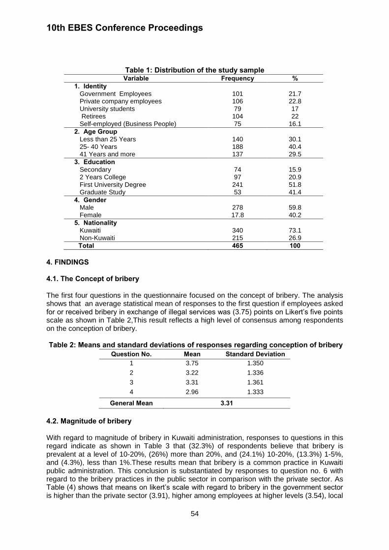
10th EBES Conference Proceedings
54
Table 1: Distribution of the study sample Variable Frequency %
1. Identity Government Employees Private company employees University students Retirees Self-employed (Business People)
101 106 79 104 75
21.7 22.8 17 22
16.1
2. Age Group Less than 25 Years 25- 40 Years 41 Years and more
140 188 137
30.1 40.4 29.5
3. Education Secondary 2 Years College First University Degree Graduate Study
74 97 241 53
15.9 20.9 51.8 41.4
4. Gender Male Female
278 17.8
59.8 40.2
5. Nationality Kuwaiti Non-Kuwaiti
340 215
73.1 26.9
Total 465 100
4. FINDINGS 4.1. The Concept of bribery The first four questions in the questionnaire focused on the concept of bribery. The analysis shows that an average statistical mean of responses to the first question if employees asked for or received bribery in exchange of illegal services was (3.75) points on Likert’s five points scale as shown in Table 2,This result reflects a high level of consensus among respondents on the conception of bribery.
Table 2: Means and standard deviations of responses regarding conception of bribery
Question No. Mean Standard Deviation 1 3.75 1.350
2 3.22 1.336 3 3.31 1.361 4 2.96 1.333
General Mean 3.31 4.2. Magnitude of bribery With regard to magnitude of bribery in Kuwaiti administration, responses to questions in this regard indicate as shown in Table 3 that (32.3%) of respondents believe that bribery is prevalent at a level of 10-20%, (26%) more than 20%, and (24.1%) 10-20%, (13.3%) 1-5%, and (4.3%), less than 1%.These results mean that bribery is a common practice in Kuwaiti public administration. This conclusion is substantiated by responses to question no. 6 with regard to the bribery practices in the public sector in comparison with the private sector. As Table (4) shows that means on likert’s scale with regard to bribery in the government sector is higher than the private sector (3.91), higher among employees at higher levels (3.54), local
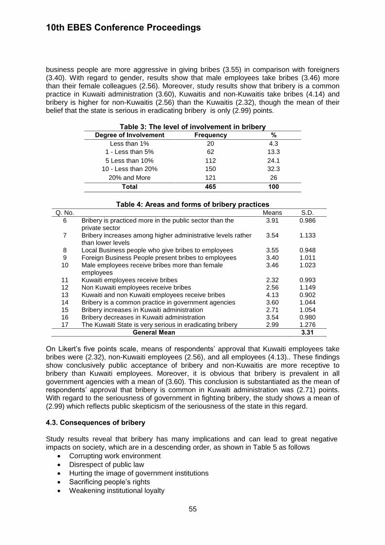
10th EBES Conference Proceedings
55
business people are more aggressive in giving bribes (3.55) in comparison with foreigners (3.40). With regard to gender, results show that male employees take bribes (3.46) more than their female colleagues (2.56). Moreover, study results show that bribery is a common practice in Kuwaiti administration (3.60), Kuwaitis and non-Kuwaitis take bribes (4.14) and bribery is higher for non-Kuwaitis (2.56) than the Kuwaitis (2.32), though the mean of their belief that the state is serious in eradicating bribery is only (2.99) points.
Table 3: The level of involvement in bribery
% Frequency Degree of Involvement 4.3 20 Less than 1% 13.3 62 1 - Less than 5%
24.1 112 5 Less than 10% 32.3 150 10 - Less than 20%
26 121 20% and More
100 465 Total
Table 4: Areas and forms of bribery practices Q. No. Means S.D.
6 Bribery is practiced more in the public sector than the private sector
3.91 0.986
7 Bribery increases among higher administrative levels rather than lower levels
3.54 1.133
8 Local Business people who give bribes to employees 3.55 0.948 9 Foreign Business People present bribes to employees 3.40 1.011 10 Male employees receive bribes more than female
employees 3.46 1.023
11 Kuwaiti employees receive bribes 2.32 0.993 12 Non Kuwaiti employees receive bribes 2.56 1.149 13 Kuwaiti and non Kuwaiti employees receive bribes 4.13 0.902 14 Bribery is a common practice in government agencies 3.60 1.044 15 Bribery increases in Kuwaiti administration 2.71 1.054 16 Bribery decreases in Kuwaiti administration 3.54 0.980 17 The Kuwaiti State is very serious in eradicating bribery 2.99 1.276
General Mean 3.31 On Likert’s five points scale, means of respondents’ approval that Kuwaiti employees take bribes were (2.32), non-Kuwaiti employees (2.56), and all employees (4.13).. These findings show conclusively public acceptance of bribery and non-Kuwaitis are more receptive to bribery than Kuwaiti employees. Moreover, it is obvious that bribery is prevalent in all government agencies with a mean of (3.60). This conclusion is substantiated as the mean of respondents’ approval that bribery is common in Kuwaiti administration was (2.71) points. With regard to the seriousness of government in fighting bribery, the study shows a mean of (2.99) which reflects public skepticism of the seriousness of the state in this regard. 4.3. Consequences of bribery Study results reveal that bribery has many implications and can lead to great negative impacts on society, which are in a descending order, as shown in Table 5 as follows
Corrupting work environment
Disrespect of public law
Hurting the image of government institutions
Sacrificing people’s rights
Weakening institutional loyalty

10th EBES Conference Proceedings
56
Poor corporate performance
Weakening sense of citizenship
Table 5: Consequences of bribery Q. No. Consequences Mean S.D.
26 Poor corporate performance 4.4989 0.66994 27 Corrupting work Environment 4.6215 0.61129 28 Weakening institutional loyalty 4.5075 0.74020 29 Hurting the image of government institutions 4.5699 0.70707 30 Weakening sense of citizenship 4.3957 0.82940 31 Loss of citizens' rights 4.5570 0.72922 32 Disrespect of public law 4.6172 0.68207
General Mean 4.53 High means of respondents’ approval of negative consequences of bribery reflects strong public belief how harmful bribery can be on society on all fronts which necessitates serious efforts to eradicate this phenomenon. The above mentioned results with regard to the four researched dimensions of bribery reveal, as shown in Table (6), are compatible as the overall statistical means were (3.31) for conception, (3.33) magnitude, (4.00) reasons, and (4.53) consequences of bribery on Likert’s five points scale.
Table 6: Means and standard deviations of the various dimensions of bribery
Bribery Dimensions Conception Magnitude Reasons Consequences
Mean 3.31 3.33 4.00 4.53
S.D. 0.965 0.451 0.568 0.527
4.4. Government employees engaged in bribery Study results show in a descending order public officials who take bribes work, as shown in the Table 7, in the following government agencies Customs and Tax Administrations, Ministry of Interior, Ministry of Municipality, Ministry of Finance and related departments, Department of Prisons, Departments of Real Estate, Department of Tenders and Procurement practices, Ministry of Education and related Institutions, Judiciary / Prosecution, and Ministry of Information and related Departments
Table 7: Frequencies and percentages of respondents regarding government Employees who take bribes
Rank Government Agency Frequency % 1 Customs and tax Agencies 367 78.9 2 Ministry of Interior 366 78.7 3 Ministry of Municipality 365 78.5 4 Departments of Purchase, Tenders, and Practices 360 77.4 5 Ministry of Finance 359 77.2 6 Department of Prisons 357 76.8 7 Department of Real estate Registration 354 76.1 8 Ministry of Education 351 75.5 9 Judiciary, Prosecutors 347 74.6
10 Media Institutions 345 74.2

10th EBES Conference Proceedings
57
4.5. Admitting bribery practices Study results as shown in Table (8) show that (14.8%) of respondents admit that they paid bribes to employees, (78.7%) never paid bribes, and (6.5%) did not answer the question. These results indicate that bribery is a common practice in Kuwaiti administration.
Table 8: Admitting paying bribes
% Number Engagements in Bribe
14.8 69 Paid Bribes 78.7 366 Did not Pay Bribes 6.5 30 No Answer 100 465 Total
4.6. Ways of Knowing about bribery Study results, as shown in Table(9),indicate that (12.7%) of respondents mention that government officials demanded bribe, (40.9%) knew about bribes from others, and (3.1%) took the initiative to pay bribes to facilitate their transactions, and (43%) did not know about bribery.
Table 9: Ways of knowing about bribes % Number How knew that I have to Pay Bribes
13.1 61 From Employees 40.9 190 From Ordinary People 3.0 14 By Myself 43.0 200 Did not Pay Bribe 100 465 Total
With regard to the amounts paid as bribes, study results, as shown in Table (10), reveal that (4.5%) of respondents mentioned that they paid less 10 KD, (1.7%), (10-20 KD), (6.9%) (20-50) KD, and (7.7%) more than (50) KD. Findings show that (7.7%) of respondents paid more than (50 d. K), and(6.9%) paid (20-50) KD.
Table 10: Amounts of bribes
% Number Amount in KD 78.7 366 Did not Pay 4.7 22 Less than 10 KDs 1.9 9 10- Less than 20 KDs 6.9 32 20 – Less than 50 KDs 7.7 36 50 KDs or more 100 465 Total
With respect to previous knowledge of those who paid bribes that this is unlawful and constitutes a crime, the study, as shown in Table(11),indicates that (77.8%) of respondents knew that bribery is illegal, ( 9.9%) did not know that bribery is illegal, and (12.3%) did not answer the question.
Table 11: Previous knowledge that bribe is Illegal % Number Knowing that Bribe is illegal
77.8 362 Know 9.9 46 Do not know 12.3 57 Not sure 100 465 Total

10th EBES Conference Proceedings
58
Study findings show that (77.8%) of respondents knew that paying bribe is a crime but nevertheless paid bribes which reflect social tolerance of bribery. 4.7. Reasons for Bribery With regard to reasons of bribery in Kuwaiti administration, the study identifies as shown in Table (12), many reasons which are, in a descending order, Lack of religious faith, weak control, Greed, Lack of legal penalties, Complication of procedures and red tape, Social tolerance of bribery, Lack of legal Education, and Low income.
Table 12: Reasons of bribery Q. No. Reason Mean S.D.
18 Weak of Control 4.3677 0.80692
19 Lack of Legal Penalties 4.1355 0.99834
20 Low Income 3.6323 1.19095
21 Greed 4.1548 0.88187
22 Social Tolerance of Bribery 3.6968 1.14681
23 Lack of adherence to religious values 4.4882 0.82287
24 Lack of Legal Education 3.6946 1.14718
25 Complicated Procedures and Red Tape
3.8860 1.16427
General Mean 2.98 4.8. Bribery and personal characteristics In order to see relationships between bribery and personal characteristics correlation analysis was conducted. The analysis revealed as Table 13 shows weak positive relationships between gender, magnitude, reasons and negative relationships with conception and effect of bribery. To examine whether bribery varies with personal characteristics, ONE WAY ANOVA was conducted. As shown in Table 15, the conception of bribery only varies at a statistically significant level among respondents according to gender but not its magnitude, reasons, or consequences.
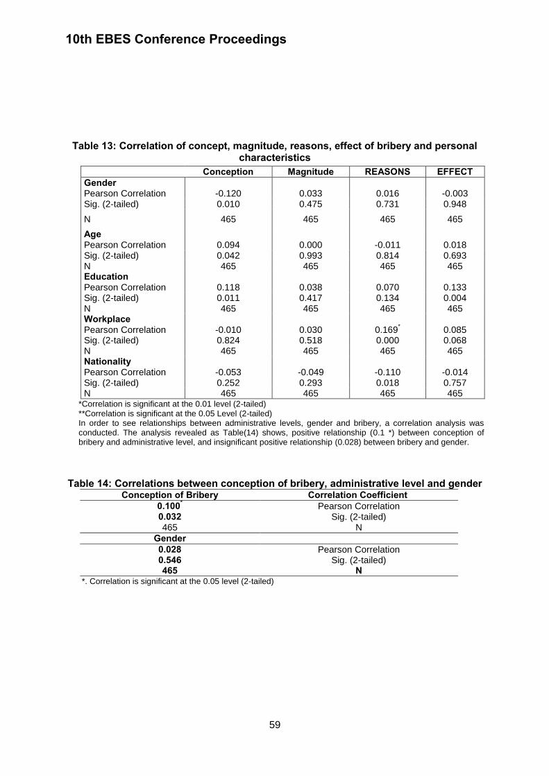
10th EBES Conference Proceedings
59
Table 13: Correlation of concept, magnitude, reasons, effect of bribery and personal characteristics
*Correlation is significant at the 0.01 level (2-tailed) **Correlation is significant at the 0.05 Level (2-tailed) In order to see relationships between administrative levels, gender and bribery, a correlation analysis was conducted. The analysis revealed as Table(14) shows, positive relationship (0.1 *) between conception of bribery and administrative level, and insignificant positive relationship (0.028) between bribery and gender.
Table 14: Correlations between conception of bribery, administrative level and gender
Correlation Coefficient Conception of Bribery Pearson Correlation 0.100*
Sig. (2-tailed) 0.032 N 465
Gender Pearson Correlation 0.028
Sig. (2-tailed) 0.546 N 465
*. Correlation is significant at the 0.05 level (2-tailed)
Conception Magnitude REASONS EFFECT Gender Pearson Correlation
-0.120
0.033
0.016
-0.003
Sig. (2-tailed) 0.010 0.475 0.731 0.948
N 465 465 465 465
Age Pearson Correlation
0.094
0.000
-0.011
0.018
Sig. (2-tailed) 0.042 0.993 0.814 0.693 N 465 465 465 465 Education Pearson Correlation
0.118
0.038
0.070
0.133
Sig. (2-tailed) 0.011 0.417 0.134 0.004 N 465 465 465 465 Workplace Pearson Correlation
-0.010
0.030
0.169
*
0.085
Sig. (2-tailed) 0.824 0.518 0.000 0.068 N 465 465 465 465 Nationality Pearson Correlation
-0.053
-0.049
-0.110
-0.014
Sig. (2-tailed) 0.252 0.293 0.018 0.757 N 465 465 465 465
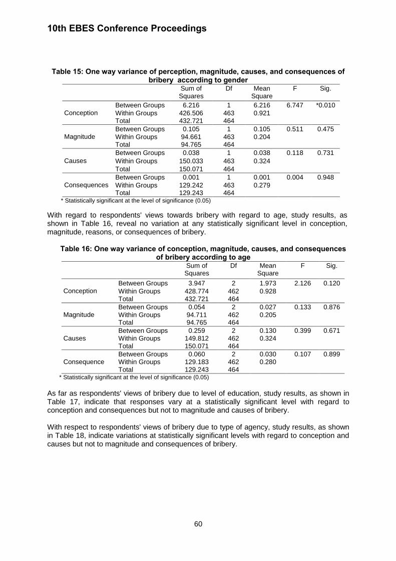
10th EBES Conference Proceedings
60
Table 15: One way variance of perception, magnitude, causes, and consequences of bribery according to gender
Sum of Squares
Df Mean Square
F Sig.
Conception Between Groups 6.216 1 6.216 6.747 *0.010
Within Groups 426.506 463 0.921 Total 432.721 464
Magnitude Between Groups 0.105 1 0.105 0.511 0.475
Within Groups 94.661 463 0.204 Total 94.765 464
Causes
Between Groups 0.038 1 0.038 0.118 0.731
Within Groups 150.033 463 0.324
Total 150.071 464
Consequences Between Groups 0.001 1 0.001 0.004 0.948
Within Groups 129.242 463 0.279 Total 129.243 464
* Statistically significant at the level of significance (0.05)
With regard to respondents' views towards bribery with regard to age, study results, as shown in Table 16, reveal no variation at any statistically significant level in conception, magnitude, reasons, or consequences of bribery.
Table 16: One way variance of conception, magnitude, causes, and consequences
of bribery according to age Sum of
Squares Df Mean
Square F Sig.
Conception Between Groups 3.947 2 1.973 2.126 0.120
Within Groups 428.774 462 0.928 Total 432.721 464
Magnitude Between Groups 0.054 2 0.027 0.133 0.876 Within Groups 94.711 462 0.205 Total 94.765 464
Causes Between Groups 0.259 2 0.130 0.399 0.671 Within Groups 149.812 462 0.324 Total 150.071 464
Consequence Between Groups 0.060 2 0.030 0.107 0.899 Within Groups 129.183 462 0.280 Total 129.243 464
* Statistically significant at the level of significance (0.05)
As far as respondents' views of bribery due to level of education, study results, as shown in Table 17, indicate that responses vary at a statistically significant level with regard to conception and consequences but not to magnitude and causes of bribery. With respect to respondents' views of bribery due to type of agency, study results, as shown in Table 18, indicate variations at statistically significant levels with regard to conception and causes but not to magnitude and consequences of bribery.
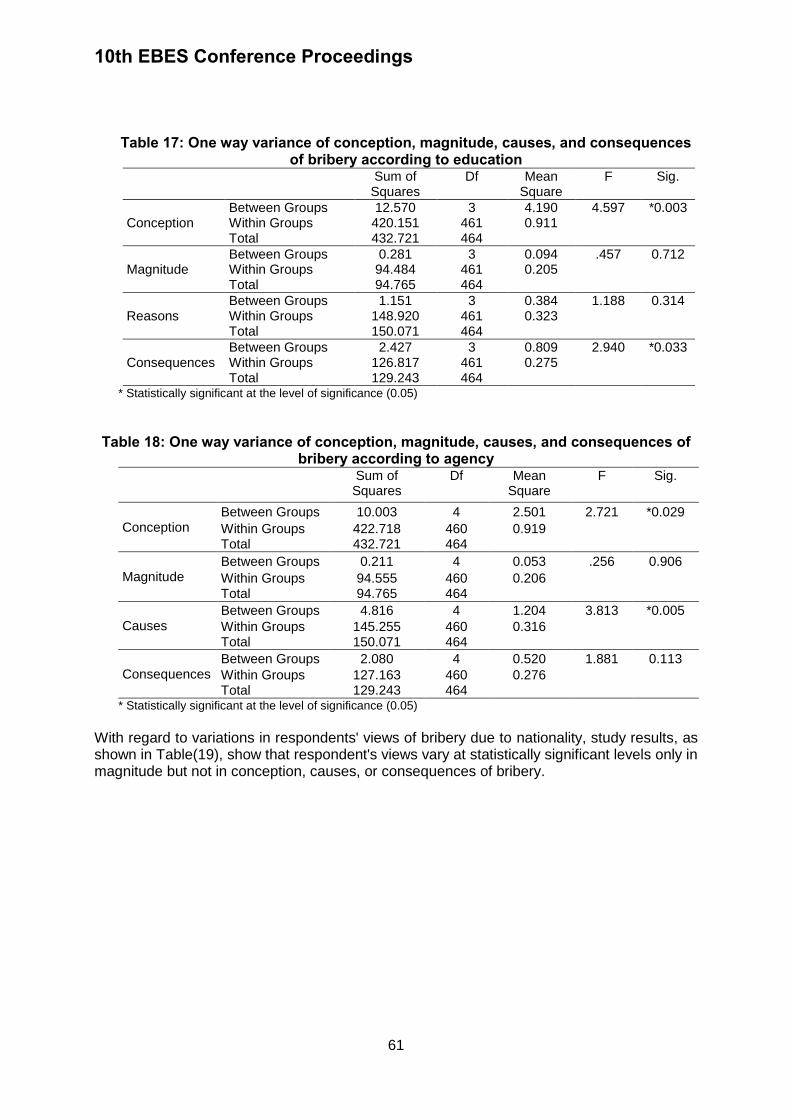
10th EBES Conference Proceedings
61
Table 17: One way variance of conception, magnitude, causes, and consequences of bribery according to education
Sum of Squares
Df Mean Square
F Sig.
Conception Between Groups 12.570 3 4.190 4.597 *0.003 Within Groups 420.151 461 0.911 Total 432.721 464
Magnitude Between Groups 0.281 3 0.094 .457 0.712 Within Groups 94.484 461 0.205 Total 94.765 464
Reasons Between Groups 1.151 3 0.384 1.188 0.314 Within Groups 148.920 461 0.323 Total 150.071 464
Consequences Between Groups 2.427 3 0.809 2.940 *0.033 Within Groups 126.817 461 0.275 Total 129.243 464
* Statistically significant at the level of significance (0.05)
Table 18: One way variance of conception, magnitude, causes, and consequences of bribery according to agency
Sum of Squares
Df Mean Square
F Sig.
Conception Between Groups 10.003 4 2.501 2.721 *0.029
Within Groups 422.718 460 0.919 Total 432.721 464
Magnitude Between Groups 0.211 4 0.053 .256 0.906
Within Groups 94.555 460 0.206 Total 94.765 464
Causes Between Groups 4.816 4 1.204 3.813 *0.005
Within Groups 145.255 460 0.316 Total 150.071 464
Consequences Between Groups 2.080 4 0.520 1.881 0.113
Within Groups 127.163 460 0.276 Total 129.243 464
* Statistically significant at the level of significance (0.05)
With regard to variations in respondents' views of bribery due to nationality, study results, as shown in Table(19), show that respondent's views vary at statistically significant levels only in magnitude but not in conception, causes, or consequences of bribery.
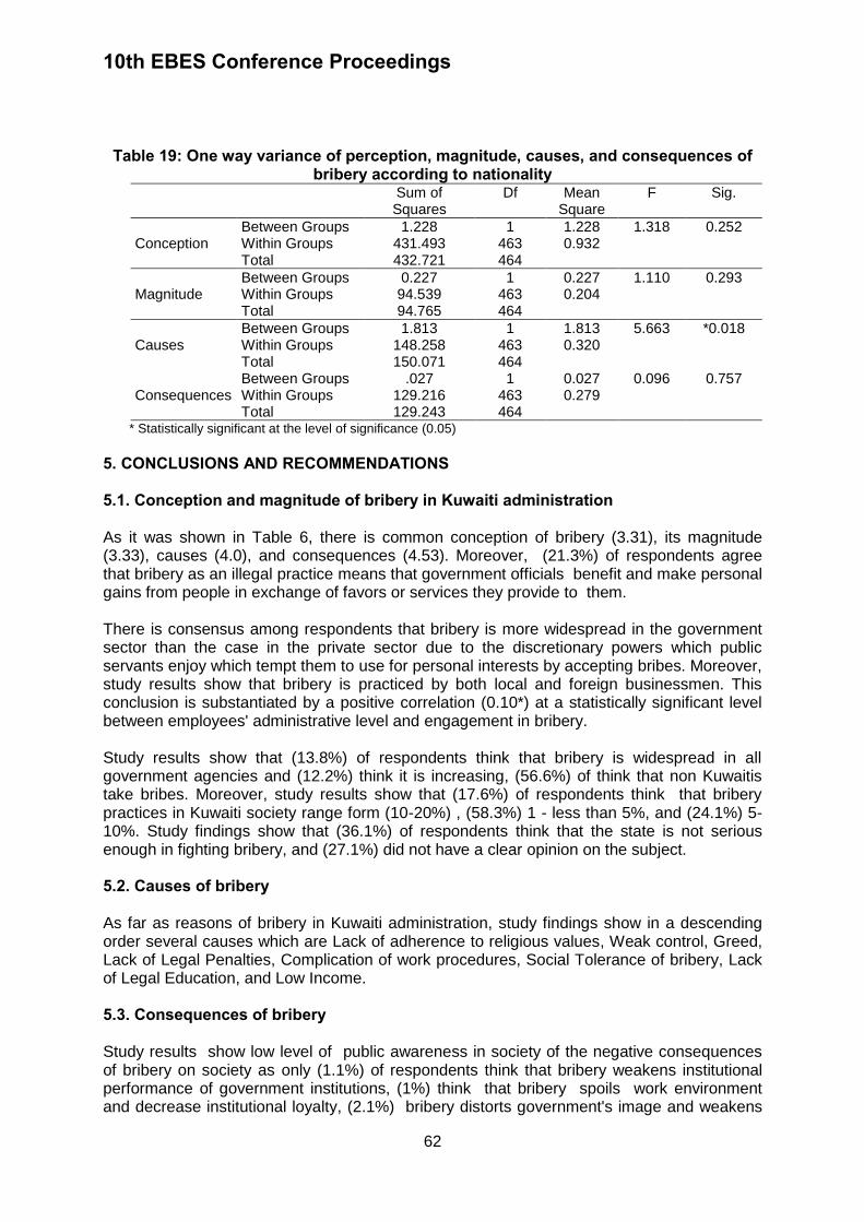
10th EBES Conference Proceedings
62
Table 19: One way variance of perception, magnitude, causes, and consequences of bribery according to nationality
Sum of Squares
Df Mean Square
F Sig.
Conception Between Groups 1.228 1 1.228 1.318 0.252 Within Groups 431.493 463 0.932 Total 432.721 464
Magnitude Between Groups 0.227 1 0.227 1.110 0.293 Within Groups 94.539 463 0.204 Total 94.765 464
Causes Between Groups 1.813 1 1.813 5.663 *0.018 Within Groups 148.258 463 0.320 Total 150.071 464
Consequences Between Groups .027 1 0.027 0.096 0.757 Within Groups 129.216 463 0.279 Total 129.243 464
* Statistically significant at the level of significance (0.05)
5. CONCLUSIONS AND RECOMMENDATIONS 5.1. Conception and magnitude of bribery in Kuwaiti administration As it was shown in Table 6, there is common conception of bribery (3.31), its magnitude (3.33), causes (4.0), and consequences (4.53). Moreover, (21.3%) of respondents agree that bribery as an illegal practice means that government officials benefit and make personal gains from people in exchange of favors or services they provide to them. There is consensus among respondents that bribery is more widespread in the government sector than the case in the private sector due to the discretionary powers which public servants enjoy which tempt them to use for personal interests by accepting bribes. Moreover, study results show that bribery is practiced by both local and foreign businessmen. This conclusion is substantiated by a positive correlation (0.10*) at a statistically significant level between employees' administrative level and engagement in bribery. Study results show that (13.8%) of respondents think that bribery is widespread in all government agencies and (12.2%) think it is increasing, (56.6%) of think that non Kuwaitis take bribes. Moreover, study results show that (17.6%) of respondents think that bribery practices in Kuwaiti society range form (10-20%) , (58.3%) 1 - less than 5%, and (24.1%) 5-10%. Study findings show that (36.1%) of respondents think that the state is not serious enough in fighting bribery, and (27.1%) did not have a clear opinion on the subject. 5.2. Causes of bribery As far as reasons of bribery in Kuwaiti administration, study findings show in a descending order several causes which are Lack of adherence to religious values, Weak control, Greed, Lack of Legal Penalties, Complication of work procedures, Social Tolerance of bribery, Lack of Legal Education, and Low Income. 5.3. Consequences of bribery Study results show low level of public awareness in society of the negative consequences of bribery on society as only (1.1%) of respondents think that bribery weakens institutional performance of government institutions, (1%) think that bribery spoils work environment and decrease institutional loyalty, (2.1%) bribery distorts government's image and weakens

10th EBES Conference Proceedings
63
sense of national belonging, (2.4%) think it sacrifices public interest and private rights, and (2.1%) think its contributes to the dissemination of a culture of disrespect for the law. 5.4. Which government agencies are engaged in bribery Study findings show categories of employees which were involved in bribery practices. These categories which are in different types of government agencies are Departments of Customs and Tax, Ministry of Interior, Ministry of Municipality, Ministry of Financial and related departments, Department of Prisons, Department of Real Estate, Department of Tenders and Procurement Practices, Ministry of Education, Judiciary / Prosecution departments, and Ministry of Information and related departments. 5.5. Ways of knowing about bribery Study results show that 12.7% of respondents mention that employees asked them directly to pay bribes, (40.9%) knew from others that they need to pay bribes, (3.1%) reported that they themselves offered employees bribes to facilitate their transactions, and (43%) did not go through the experience of bribery. With regard to amounts paid as bribes, study results showed that (4.5%) of respondents mentioned that they paid less than ten KD, (1.7%) (10-20 KD), (6.9%) (20-50) KD, and (7.7%) paid more than (50) KD. This shows that the largest percentage of those who paid a bribe (7.7%) paid more than (50 KD), followed respectively (6.9%) by those who paid (20-50) KDs. 5. 6. Knowledge of illegality of bribery Study results show that (77.8%) of respondents mention that they knew that bribery is a crime punishable by law, (9.9%) did not know that it was a crime, and (12.3%) did not respond. These results show that Kuwaiti society tolerates bribery and does not see it a serious problem. 5.7. Personal characteristics and bribery With regard to the relationships between personal variables and bribery, study findings show that respondents view on bribery do not vary due to gender but only in its conception. This might be explained by prevailing cultural norms which make men have more access to bribery practices than women. Likewise, variations at statistical significant levels were found in respondents' views only on the conception and consequences but not on magnitude and causes of bribery according to education level. This can be explained as highly educated respondents are more aware of bribery practices and its negative results on society than less educated employee. As far as nationality is concerned, study results show that respondent's views vary at statistically significant levels only in their view of magnitude of bribery but not in its conception, causes, or consequences. This might be explained because Kuwaitis have more access to information regarding bribery practices than non-Kuwaitis. 6. Conclusion and Recommendations In the light of study findings, some recommendations can be suggested. Government agencies have to exert intensive efforts to raise public awareness of the seriousness of bribery and its negative repercussions on society. Such efforts are of prime importance at a time where Arab countries face social and political unrest which represent the most serious manifestations against corruption, injustice, inequity and bribery which come on top list of slogans in demonstrations against governments. The role of media and religious institutions
10th EBES Conference Proceedings
64
are of prime importance in this regard as the study shows social tolerance of bribery and lack of adherence to religious values. It is important to hold a national conference on the problem of bribery in Kuwait to shed light on this problem them and discuss way to eradicate this serious problem. Conducting training programs, seminars, workshops which focus on bribery as a crime and its adverse effects on the image of the government and its employees and on society at large are necessary. This is important in view of study findings of positive relationship between administrative level and bribery, which hold top administration a special responsibility to address this problem. It may be important to reconsider salary scales for non-Kuwaitis as study findings show that 56.6% of respondents mention that non Kuwaitis take bribe and one reason for this is low income. It is illogical to discriminate in salaries paid for the same job as this might be taken as justifications for taking bribes. Government agencies must simplify procedures, prepare and distribute brochures to service recipients stating their access rights to services, and specify documents, conditions, and time needed for getting the service, and what they can do in the event of a delay of service. This would reduce people's resort to pay bribes to get services. This is important because study findings show that people's ignorance of their rights besides complicated procedures come in the third and fourth ranks as reasons for paying bribes. Reconsideration of legislations which relate to the penalties for bribery and tightening sanctions, as study findings show that despite the majority of employees learned that receiving bribery is illegal but nevertheless they take bribes. This explains the lack of deterrent penalties which came in fifth place as one of the reasons of bribery. Tightening internal and external government control and lawful penalties for employees who take bribes because study findings show that the weak oversight comes as the sixth cause of bribery. REFERENCES Aidt, T.S. 2003. Economic analysis of corruption: A survey. Economic Journal. 11(491), pp.632-652. Caselli, F. 2005. Accounting for cross-country income differences. In: P. Aghion and S. Durlauf, eds. Handbook of economic growth. Amsterdam: Elsevier. Jain, A.K., 2001. Corruption: A review. Journal of Economic Surveys. 15(1), pp.71-211. Lambsdorff, J.G. 2003. How corruption affects productivity. Kyklos. 56(4), pp.457-474. Meon, P.G. and Weill, L., 2005. Does better governance foster efficiency? An Aggregate Frontier Analysis. Economics of Governance, 6(1), pp.75-90. Nwabuzor, A., 2005. Corruption and development: New, initiatives in economic openness and strengthened rule of law. Journal of Business Ethics, 59(1-2), pp.121-138.
10th EBES Conference Proceedings 23 - 25 May, 2013. NIPPON HOTEL, ISTANBUL, TURKEY ISBN: 978-605-64002-1-6. WEBSITE: www.ebesweb.org
65
CYCLICAL FLUCTUATIONS AND CREDIT RISK MANAGEMENT IN ITALY IN THE PERIOD 2008-2012: A
BIOSTATISTICAL APPROACH
STEFANO OLGIATI Department of Management, Economics and Quantitative Methods
University of Bergamo Italy
ALESSANDRO DANOVI Department of Management, Economics and Quantitative Methods
University of Bergamo Italy
[email protected] Abstract: From June 2008 to June 2012, Credit risk management in Italy was characterized by frequent and intense quarterly contractions and expansions around the mean of the nominal total credit used by non-financial corporations. Such fluctuations are frequently ascribed to exogenous Basel II procyclical effects on credit flow into the economy and, consequently, Basel III output-based point-in-time Credit/GDP countercyclical buffering. We have tested the opposite null hypotheses that such variation is correlated to actual default rates, and that such correlation is explained by fluctuations of credit supply around a steady state. We have found that, between June 2008 – and June 2012 (n=17), linear regression of credit growth rates on default rates revealed a negative correlation and that credit supply fluctuated steadily around the default rate with a Steady State Parameter SSP=.00245 with χ2=.3747. We conclude that credit risk management in Italy has been effective in parameterising the credit supply variation to default rates within the Basel II operating framework. Basel III prospective countercyclical point-in-time output buffers based on filtered Credit/GDP ratios and dynamic provisioning proposals should take into account this underlying steady state statistics pattern. Keywords: Frequent Cyclical Fluctuations, Credit Growth Rate, Default Rate, Retrospective Forecasting, Steady State Function, Cyclical Sensitivity Parameter 1. BACKGROUND Credit risk management has become one of the most relevant topics both for financial institutions and for scholars. Credit risk models have evolved from subjective analysis to accounting-based credit-scoring systems and measures of credit risk and risk concentration (Altman and Saunders, 1998) and their effects on capital allocation and shareholders’ value in banking assessed (Resti and Sironi 2012). The European Commission with the Credit Risk Directives (CRD I, II and III) and Banking Authorities with Basel Accords on minimum capital requirements and countercyclical buffers (Basel II and III) are still carrying out a long process of formalization of credit risk management methods and guidelines in order to diffuse a culture of common rules at the continental level.
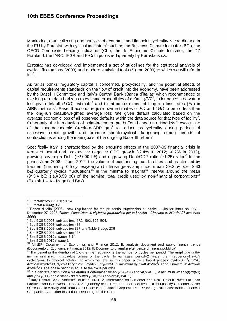
10th EBES Conference Proceedings
66
Monitoring, data collecting and analysis of economic and financial cyclicality is coordinated in the EU by Eurostat, with cyclical indicators1 such as the Business Climate Indicator (BCI), the OECD Composite Leading Indicators (CLI), the Ifo Economic Climate Indicator, the DZ Euroland, the IARC, IESR and E-Coin published quarterly by Eurostatistics. Eurostat has developed and implemented a set of guidelines for the statistical analysis of cyclical fluctuations (2003) and modern statistical tools (Sigma 2009) to which we will refer in full2. As far as banks’ regulatory capital is concerned, procyclicality, and the potential effects of capital requirements standards on the flow of credit into the economy, have been addressed by the Basel II Committee and Italy’s Central Bank (Banca d’Italia)3 which recommended to use long term data horizons to estimate probabilities of default (PD)4, to introduce a downturn loss-given-default (LGD) estimate5 and to introduce expected long-run loss rates (EL) in AIRB methods6. Basel II accords require own estimates of PD and LGD to be no less than the long-run default-weighted average loss rate given default calculated based on the average economic loss of all observed defaults within the data source for that type of facility7. Coherently, the introduction of point-in-time output buffers based on a Hodrick-Prescott filter of the macroeconomic Credit-to-GDP gap8 to reduce procyclicality during periods of excessive credit growth and promote countercyclical dampening during periods of contraction is among the main goals of the ongoing Basel III reform9. Specifically Italy is characterized by the enduring effects of the 2007-09 financial crisis in terms of actual and prospective negative GDP growth (-2.4% in 2012; -0.2% in 2013), growing sovereign Debt (≅2,000 b€) and a growing Debt/GDP ratio (≅1.25) ratio10 In the period June 2008 – June 2012, the volume of outstanding loan facilities is characterized by frequent (frequency=0.5 cycles/year) and intense (peak amplitude: mean=39.2 b€; s.e.=2.83 b€) quarterly cyclical fluctuations11 in the minima to maxima12 interval around the mean (915.4 b€; s.e.=3.59 b€) of the nominal total credit used by non-financial corporations13 (Exhibit 1 – A - Magnified Box).
1 Eurostatistics 12/2012: 9-14
2 Eurostat (2003); 3.2
3 Banca d’Italia (2006), New regulations for the prudential supervision of banks - Circular letter no. 263 -
December 27, 2006 (Nuove disposizioni di vigilanza prudenziale per le banche - Circolare n. 263 del 27 dicembre 2006) 4 See BCBS 2006, sub-sections 472, 502, 503, 504.
5 See BCBS 2006, sub-section 468
6 See BCBS 2006, sub-section 367 and Table 6 page 236
7 See BCBS 2006, sub-section 468
8 See BCBS 2010a, pages 8-14
9 See BCBS 2010a, page 1
10 MINEF, Document of Economics and Finance 2012, II: analysis document and public finance trends
(Documento di Economia e Finanza 2012, II: Documento di analisi e tendenze di finanza pubblica) 11
If a period is the duration of 1 cycle, the frequency is the number of cycles per period. The amplitude is the minima and maxima absolute values of the cycle. In our case: period=2 years, then frequency=1/2=0.5 cycles/year. In physical notation, to which we refer in this paper, a cycle has 4 phases: dy/dx>0 d
2y/dx
2>0,
dy/dx>0 d2y/dx
2<0, dy/dx<0 d
2y/dx
2<0, dy/dx<0 d
2y/dx
2>0, 1 minimum dy/dx=0 d
2y/dx
2>0 and 1 maximum dy/dx=0
d2y/dx
2<0. The phase period is equal to the cycle period/4.
12 In a discrete distribution a maximum is determined when y(t)>y(t-1) and y(t)>y(t+1), a minimum when y(t)<y(t-1)
and y(t)<y(t+1) and a steady state when y(t)=y(t-1) and/or y(t)=y(t+1). 13
Italy Central Bank, Statistical Bulletin III-2012, Information on Customer and Risk, Default Rates For Loan Facilities And Borrowers, TDB30486: Quarterly default rates for loan facilities - Distribution By Customer Sector Of Economic Activity And Total Credit Used: Non-financial Corporations - Reporting Institutions: Banks, Financial Companies And Other Institutions Reporting To The Ccr.

10th EBES Conference Proceedings
67
The conflicting effects of cyclicality on the tradeoff between stability and timeliness in predicting probabilities of default and recovery rates have been analyzed by Altman, Brady, Sironi and Resti (2005), who observe that banks tend to react to short-term evidence therefore regulation should encourage the use of long-term average rates in AIRB systems. In Italy linear long-term predictions due to the frequent cyclical waveform fluctuation are statistically significant (ŷ≅y and dŷ/dx≅dy/dx) only every 8 quarters (4 phases, 2 years). Altman and Rijiken (2005) observe that agencies delay the timing of through the cycle rating migration estimates by 0.56 years at the downside and 0.79 years at the upside. This signifies that in Italy, with a phase period of 0.5 years, as we will see, in a period of economic downturn, agency ratings are systematically one phase late through the cycle. Jarrow et al. (1997) provide a discrete time-homogeneous Markov chain transition matrix for the term structure of credit risk spreads which assumes a time step of one year. In Italy in the period 2008-2012 this time step corresponds to two phases of the cycle (1 year), rendering the assumption of time-homogeneity during such time step not statistically acceptable. Gordy and Howells (2004) observe that credit risk adjusted portfolio management is based on time-homogeneous Markov transition processes, which are based on ex-ante probabilities of default which register all expected variation in the rating variables and register all ex-post variation as unexpected. Frequent cyclicality would systematically alter the ratio between unexpected and expected variation. Repullo et al. (2008, 2009, 2011) observe that higher buffers in expansions are insufficient to prevent a significant contraction in the supply of credit at the arrival of a recession, which in Italy has occurred in the period 2008-2012 every year. Sironi and Resti (2012) observe that a modification of the current IFRS 39 concept of incurred loss with a principle of fair value and amortized cost could further increase the procyclicality of banks’ credit policies. In Italy, 0.5-year phases render misleading through-the-cycle quarterly and half year estimates of fair values. 2. RESEARCH QUESTIONS AND METHODS In this paper we have asked two research questions: Q1 – is there a statistically significant linear relationship linking credit output fluctuations to default rates in the period June 2008 – June 2012? We argue that if such a linear relationship does exist or, in other words, if variation in credit supply is satisfactorily explained by independent variation in the default rates then, given the a priori postulate that exogenous macro-conditions, such as the business cycle, do affect default rates and Basel II minimum capital requirements do have procyclical effects, then such exogenous effects are satisfactorily transformed by the endogenous relationship between credit and default rates, as it should be according to operating Basel II Accords. In other words, if the relationship is linear (d2y/dx2=0) it is not procyclical (d2y/dx2≠0); Q2 – given that Q1 linear relationship does exist, can we formulate a null hypothesis regarding the causes of such relationship which can be statistically analyzed and tested? In particular we will test the hypothesis that credit supply variation systematically converges to a steady state, i.e. credit supply is systematically increased or decreased in order to achieve credit steady state at a certain level. We have analyzed Italy’s Central Bank Statistical Bulletin’s quarterly default rates for loan
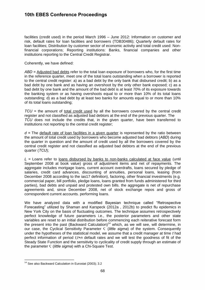
10th EBES Conference Proceedings
68
facilities (credit used) in the period March 1996 – June 2012: Information on customer and risk, default rates for loan facilities and borrowers (TDB30486); Quarterly default rates for loan facilities; Distribution by customer sector of economic activity and total credit used: Non-financial corporations; Reporting institutions: Banks, financial companies and other institutions reporting to the Central Credit Registrar. Coherently, we have defined: ABD = Adjusted bad debts refer to the total loan exposure of borrowers who, for the first time in the reference quarter, meet one of the total loans outstanding when a borrower is reported to the central credit register: a) as a bad debt by the only bank that disbursed credit; b) as a bad debt by one bank and as having an overshoot by the only other bank exposed; c) as a bad debt by one bank and the amount of the bad debt is at least 70% of its exposure towards the banking system or as having overshoots equal to or more than 10% of its total loans outstanding; d) as a bad debt by at least two banks for amounts equal to or more than 10% of its total loans outstanding; TCU = the amount of total credit used by all the borrowers covered by the central credit register and not classified as adjusted bad debtors at the end of the previous quarter. The TCU does not include the credits that, in the given quarter, have been transferred to institutions not reporting to the central credit register; d = The default rate of loan facilities in a given quarter is represented by the ratio between the amount of total credit used by borrowers who become adjusted bad debtors (ABD) during the quarter in question and the amount of credit used by all the borrowers covered by the central credit register and not classified as adjusted bad debtors at the end of the previous quarter (TCU); L = Loans refer to loans disbursed by banks to non-banks calculated at face value (until September 2008 at book value) gross of adjustment items and net of repayments. The aggregate includes mortgage loans, current account overdrafts, loans secured by pledge of salaries, credit card advances, discounting of annuities, personal loans, leasing (from December 2008 according to the ias17 definition), factoring, other financial investments (e.g. commercial paper, bill portfolio, pledge loans, loans granted from funds administered for third parties), bad debts and unpaid and protested own bills. the aggregate is net of repurchase agreements and, since December 2008, net of stock exchange repos and gross of correspondent current accounts. performing loans. We have analyzed data with a modified Bayesian technique called “Retrospective Forecasting” utilized by Shaman and Karspeck (2012a , 2012b) to predict flu epidemics in New York City on the basis of fluctuating outcomes. The technique assumes retrospectively perfect knowledge of future parameters i.e., the posterior parameters and other state variables are reset to an initial distribution before commencing each reiterative forecast form the present into the past (Backward Calculation)14 which, as we will see, will determine, in our case, the Cyclical Sensitivity Parameter Ϛ (little sigma) of the system. Consequently
under the hypotheses of the statistical model, we assume that a credit manager at time t had perfect information of period t,t+n default rates and we will test the goodness of fit of the Steady State Function and the sensitivity to cyclicality of credit supply through an estimate of the parameter Ϛ (little sigma) with a Chi-Square Test.
14
See also Backward Calculation in Eurostat (2003); 3.2

10th EBES Conference Proceedings
69
We have assumed an LGD=1; the hypothesis is reasonable in the framework of the analysis since recovery rates affect, at time of recovery, the credit supply to the economy, and such effect will be “seen” in the total credit used and in the credit growth rate. Under these assumptions, we have defined the variable f as:
f = The credit growth rate determined as
f ;L
t ,tn
TCUt1 d
t ,tn
n
The credit growth rate is asymptotically equal to the amount of loan facilities disbursed in period t,t+n divided by the total credit used at the beginning t of the period which will survive (1-d) to the end t+n of such period. The variable f assumes that the credit risk manager possesses perfect information regarding d and therefore will not grant new loans or additional loans L to borrowers which will default in the same period; δ = The sliding time parameter δ accounts for the fact that the nearer the credit risk manager gets retrospectively to time t+n , the more perfect information becomes and thus the retrospective forecast; Ϛ = the cyclical sensitivity parameter (CSP). In other words, the CSP is determined through repeated backwards iterations as the parameter that solves the implicit Steady State Function (Equation 1) for X=d and Y=f given:
1dt ,t1 1 f
t ,t1 t0
T1
1 T1
n
; 1
(1) We can now formulate the null hypotheses that:
Q1: HQ1
0: f
1
2d
: the credit supply growth is a dependent variable linked by a linear relationship with the default rate;
Q2: HQ2
0:
d
1d; 0
: the credit supply growth or decline rate is explained by the default rate alone and is not sensitive to exogenous cyclicality. In alternative, we will test and that the credit supply growth or decline rate is not explained by the default rate alone and is sensitive to exogenous cyclical positive or negative factors. We have utilized Mathematica 8 and Statistical-Graphical Integration with Mac OS X Datagraph 3.1. 3. FINDINGS The findings are summarized in Equation 2. In synthesis, we accept the null hypothesis H0 that the frequent fluctuations of the total credit used by non-financial corporations TCU in the period June 2008-June 2012 can be explained satisfactorily with a quasi linear relationship by the independent variable “default rate”: FX={f | d} with Ϛ≈0=0.0014743 and a Chi-Square
of 0.4509 (n=17). In the preceding period March 1996-June 2008, credit has grown in excess of the period default rates at a significant and steady rate of 2.1% (Ϛ≠0=0.02068) with a Chi-
Square of 1.063 (n=49).

10th EBES Conference Proceedings
70
FX
f |d d 0.0014743
1dif t
jun08,t
mar12
d 0.02068
1dif t
mar96,t
jun08
(2) Equation 1: Steady State Function (SSF): Distribution of credit supply growth f given
the default rate d and the cyclical sensitivity parameter Ϛ All evidence, discrete distributions and statistical tests have been summarized in Exhibits 1, 2 and 3. 3.1. Exhibit 1-A The total credit used by non-financial corporations TCU in the period March 1996 – June 2012 has been divided into 2 sub-periods. The first period from March 1996 to June 2008 excluded, and the second period from June 2008 included to June 2012. The starting date of the second period has been chosen so as to comprise a total period of 4 years, the period during which the total credit used (mean=915.4 b€; s.e.=3.59 b€) reveals 8 phases (n-1 quarters) and 2 cyclical fluctuations (I and II). Real total credit utilizes as basis March 1996=100, with a yearly non-adjusted inflation of 2.06% form March 1996 to June 2008 and 1.91% form June 2008 to June 2012. 3.2. Exhibit 1-B We have divided the Credit Supply Growth Rates (f) and the Default Rates (d) of the period March 1996 – June 2012 into 2 sub-periods. The first period from March 1996 to June 2008 , and the second period from June 2008 to June 2012. The concave-upward (convex downward) quadratic fit reveals a significant (R2>0.5) R2=0.64628 for the default rate time series and linear regression a non-significant R2=0.05019 for the credit supply time series. From a time series perspective, credit growth appears stable vs. default rates declining and then growing again. 3.3. Exhibit 1-C Linear regression of credit supply rates as a function of default rates by Ordinary Least Squares (OLS) from March 1996 to June 2008 reveals a R2 = 0.0451 and �2=0.9904 (Exhibit 3). Null hypotheses H0 (lower solid line) and HI (upper solid line) testing of the observed credit growth rates vs. the expected rates following the SSF reveals a steady state parameter of Ϛ=0.02068 with a �2=1.063 (Exhibit 3). In synthesis, in the period March 1996-June 2008,
credit has grown in excess of the period default rates at a significant and steady rate of 2.1% (Ϛ≠0=0.02068) with a Chi-Square of 1.063 (n=49).
3.4. Exhibit 1-D Linear regression of credit supply rates given the default rates by OLS from June 2008 to June 2012 reveals a R2 = 0.4367 and a �2= - 0.2064 (Exhibit 3). Null hypothesis H0 (lower
solid line) testing of the observed credit supply rates vs. the expected rates following the SSF reveals a steady state parameter Ϛ=0.0014743 with a �2=0.4509 (Exhibit 3). In synthesis,
from June 2008 to June 2012, credit growth rates are linearly negatively correlated to default rates but appear to be significantly fluctuating around the Steady State Function with null cycle sensitivity.
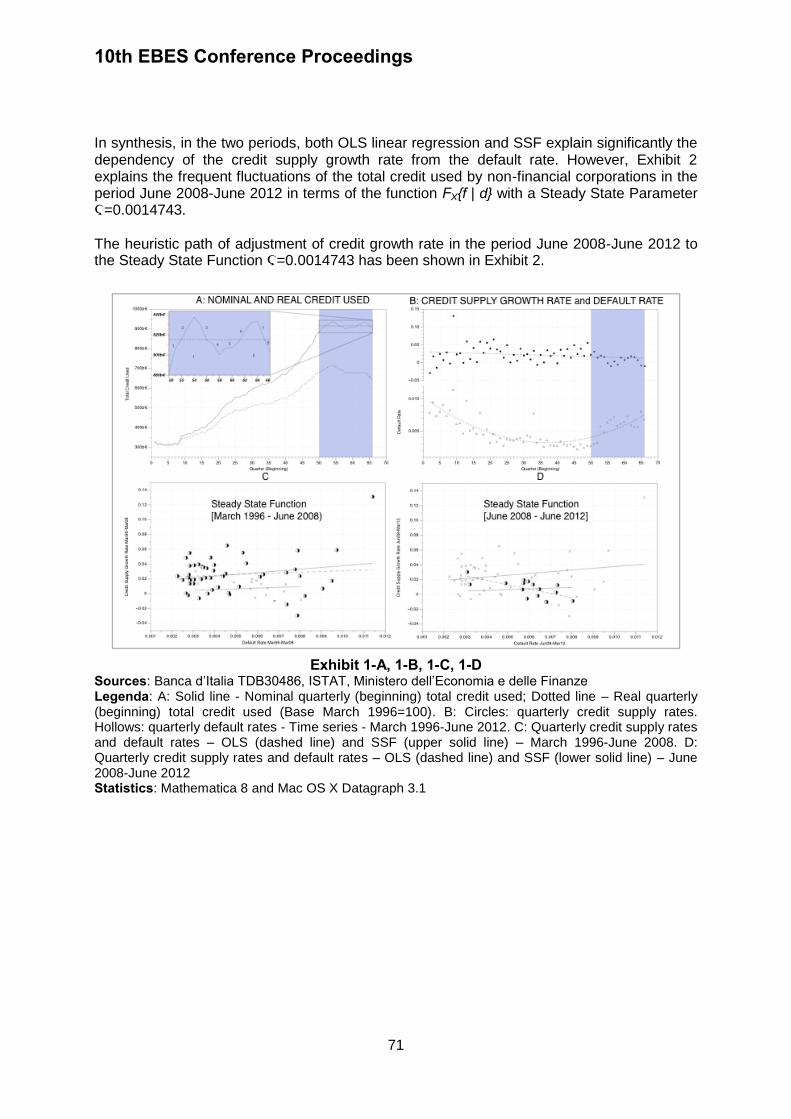
10th EBES Conference Proceedings
71
In synthesis, in the two periods, both OLS linear regression and SSF explain significantly the dependency of the credit supply growth rate from the default rate. However, Exhibit 2 explains the frequent fluctuations of the total credit used by non-financial corporations in the period June 2008-June 2012 in terms of the function FX{f | d} with a Steady State Parameter Ϛ=0.0014743.
The heuristic path of adjustment of credit growth rate in the period June 2008-June 2012 to the Steady State Function Ϛ=0.0014743 has been shown in Exhibit 2.
Exhibit 1-A, 1-B, 1-C, 1-D
Sources: Banca d’Italia TDB30486, ISTAT, Ministero dell’Economia e delle Finanze Legenda: A: Solid line - Nominal quarterly (beginning) total credit used; Dotted line – Real quarterly (beginning) total credit used (Base March 1996=100). B: Circles: quarterly credit supply rates. Hollows: quarterly default rates - Time series - March 1996-June 2012. C: Quarterly credit supply rates and default rates – OLS (dashed line) and SSF (upper solid line) – March 1996-June 2008. D: Quarterly credit supply rates and default rates – OLS (dashed line) and SSF (lower solid line) – June 2008-June 2012 Statistics: Mathematica 8 and Mac OS X Datagraph 3.1
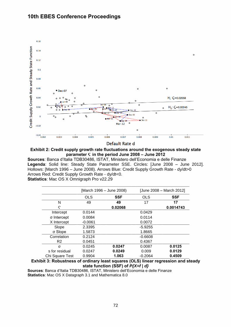
10th EBES Conference Proceedings
72
Exhibit 2: Credit supply growth rate fluctuations around the exogenous steady state parameter Ϛ in the period June 2008 – June 2012
Sources: Banca d’Italia TDB30486, ISTAT, Ministero dell’Economia e delle Finanze Legenda: Solid line: Steady State Parameter SSE. Circles: [June 2008 – June 2012]. Hollows: [March 1996 – June 2008). Arrows Blue: Credit Supply Growth Rate - dy/dt>0 Arrows Red: Credit Supply Growth Rate - dy/dt<0. Statistics: Mac OS X Omnigraph Pro v22.29
[March 1996 – June 2008) [June 2008 – March 2012]
OLS SSF OLS SSF N 49 49 17 17 Ϛ 0.02068 0.0014743
Intercept 0.0144 0.0429 σ Intercept 0.0084 0.0114 X Intercept -0.0061 0.0072
Slope 2.3395 -5.9255 σ Slope 1.5873 1.8665
Correlation 0.2124 -0.6608 R2 0.0451 0.4367 σ 0.0245 0.0247 0.0087 0.0125
s for residual 0.0247 0.0249 0.009 0.0129 Chi Square Test 0.9904 1.063 -0.2064 0.4509
Exhibit 3: Robustness of ordinary least squares (OLS) linear regression and steady state function (SSF) of P{X=f | d}
Sources: Banca d’Italia TDB30486, ISTAT, Ministero dell’Economia e delle Finanze Statistics: Mac OS X Datagraph 3.1 and Mathematica 8.0
10th EBES Conference Proceedings
73
4. INTERPRETATION Credit risk management in Italy is characterized, in the period June 2008 – June 2012, by frequent (frequency=0.5 cycles/year) and intense (peak amplitude: mean=39.2 b€; s.e.=2.83 b€) quarterly cyclical fluctuations in the minima to maxima interval around the mean (915.4 b€; s.e.=3.59 b€) of the nominal total credit used by non-financial corporations. Such frequent and intense credit output fluctuations are frequently ascribed to exogenous Basel II procyclical effects and, consequently, output-based point-in-time Credit/GDP countercyclical buffering or dynamic provisioning advocated. We have tested the opposite null hypothesis that such fluctuations in credit growth are entirely explained by a quasi-linear continuous Steady State Function (SSF) of the actual default rates parameterized with a Cyclical Sensitivity Parameter (CSP) of credit supply variation in excess or defect of the rate of defaulting loans. We have found that, in the period June 2008 – June 2012, with a CSP of 0.00147 and a Chi-Square of 0.4509 (n=17), the frequent fluctuations of the total credit used by non-financial corporations are significantly explained by variation of the independent variable “default rate”, with no significant evidence of positive or negative cyclical sensitivity of the credit supplied. We conclude that credit risk management in Italy has been effective in parameterizing credit supply growth to default rates within the Basel II operating framework. Basel III prospective countercyclical point-in-time output buffers based on filtered Credit/GDP ratios and dynamic provisioning proposals should take into account this steady state statistical pattern underlying frequent and intense credit cyclical fluctuations. 5. LIMITS As Gordy (2003) observes credit risk is idiosyncratic to the obligor, and what we define a cycle is really a composite of a multiplicity of cycles tied to location, period and sector. Therefore this model suffers from the same limits as the Credit/GDP countercyclical buffers, i.e. a single-factor model cannot capture any clustering of default rates due to dishomogeneous sensitivity to smaller-scale components of the macro cycle. REFERENCES Altman, E.I. and Saunders, A., 1996. Credit risk measurement: Developments over the last 20 years. Journal of Banking & Finance, 21(11-12), pp.1721-1742. Altman E.I. and Rijken H.A., 2005. The effects of rating through the cycle on rating stability, rating timeliness and default prediction performance. [online] Available at: <http://archive.nyu.edu/bitstream/2451/26405/2/FIN-05-004.pdf> [Accessed 23 December 2012] Altman E.I., Brady B., Resti A., and Sironi A., 2005. The link between default and recovery rates: Theory, empirical evidence and implications. Journal of Business, 78(6), pp.2203-2227. Banca d’Italia, 2006. New regulations for the prudential supervision of banks [Nuove disposizioni di vigilanza prudenziale per le banche]. Circolare no. 263. [online] Available at: <http://www.bancaditalia.it/vigilanza/normativa/norm_bi/circ-reg/vigprud> [Accessed 4 June 2013). Banca d’Italia, Statistical bulletin on-line, information on customer and risk. [online] Available at: <http://bip.bancaditalia.it/4972unix/homebipentry.htm?dadove=corr&lang=eng> [Accessed 1 January 2013].
10th EBES Conference Proceedings
74
Basel Committee on Banking Supervision, 2006. International convergence of capital measurement and capital standards. A revised framework comprehensive version. Basel: Bank for International Settlements. Basel Committee on Banking Supervision, 2010a, Guidance for national authorities operating the countercyclical capital buffer. Basel: Bank for International Settlements. Basel Committee on Banking Supervision, 2010b. Basel III: A global regulatory framework for more resilient banks and banking systems. Basel: Bank for International Settlements. Eurostat, 2003. Statistical analysis of cyclical fluctuations. Luxembourg: Office for Official Publications of the European Communities. Eurostat, 2012. Eurostatistics Statistical books - Data for short-term economic analysis. Luxembourg: Office for Official Publications of the European Communities. Gordy, M.B., 2003. A risk-factor model foundation for ratings-based bank capital rules. Journal of Financial Intermediation, 12(3), pp.199-232. Gordy, M.B. and Howells B., 2004. Procyclicality in Basel II: Can we treat the disease without killing the patient? Basel: Bank of International Settlements. Jarrow R.A., Lando D., and Turnbull S.M., 1997. A markov model for the term structure of credit risk spreads. The Review of Financial Studies. 10(2), pp.481–523. Repullo R.and J. Suarez, 2008. The procyclical effects of Basel II. CEPR Discussion Paper, 6862. Repullo R., Saurina J., and Trucharte C., 2009. Mitigating the Procyclicality of Basel II. CEMFI Working Paper, 0903 Repullo R. and Saurina J., 2011. The countercyclical capital buffer of Basel III a critical assessment. Banco de España, March. Resti A. and Sironi A., 2012. Risk management and shareholders’ value in banking. New York: Wiley. Shaman J. and Karspeck A., 2012a, Forecasting seasonal outbreaks of influenza. PNAS, 109(50), pp.20425-20430. Shaman J. and Karspeck A., 2012b. Forecasting seasonal outbreaks of influenza – Supporting Information, PNAS. Sigma, 2009. Modern tools for business cycle analysis. The bulletin of European statistics, Luxembourg: Office for Official Publications of the European Communities.
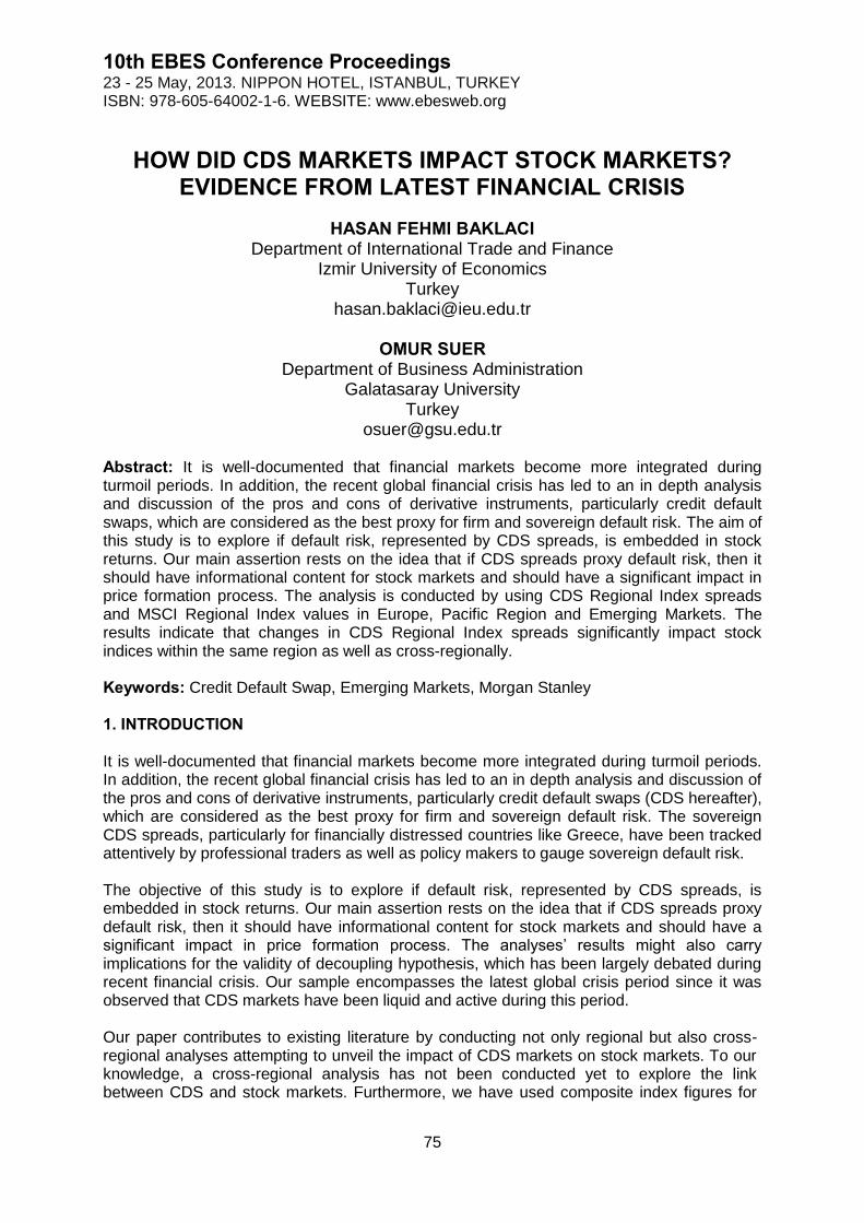
10th EBES Conference Proceedings 23 - 25 May, 2013. NIPPON HOTEL, ISTANBUL, TURKEY ISBN: 978-605-64002-1-6. WEBSITE: www.ebesweb.org
75
HOW DID CDS MARKETS IMPACT STOCK MARKETS? EVIDENCE FROM LATEST FINANCIAL CRISIS
HASAN FEHMI BAKLACI
Department of International Trade and Finance Izmir University of Economics
Turkey [email protected]
OMUR SUER
Department of Business Administration Galatasaray University
Turkey [email protected]
Abstract: It is well-documented that financial markets become more integrated during turmoil periods. In addition, the recent global financial crisis has led to an in depth analysis and discussion of the pros and cons of derivative instruments, particularly credit default swaps, which are considered as the best proxy for firm and sovereign default risk. The aim of this study is to explore if default risk, represented by CDS spreads, is embedded in stock returns. Our main assertion rests on the idea that if CDS spreads proxy default risk, then it should have informational content for stock markets and should have a significant impact in price formation process. The analysis is conducted by using CDS Regional Index spreads and MSCI Regional Index values in Europe, Pacific Region and Emerging Markets. The results indicate that changes in CDS Regional Index spreads significantly impact stock indices within the same region as well as cross-regionally. Keywords: Credit Default Swap, Emerging Markets, Morgan Stanley 1. INTRODUCTION It is well-documented that financial markets become more integrated during turmoil periods. In addition, the recent global financial crisis has led to an in depth analysis and discussion of the pros and cons of derivative instruments, particularly credit default swaps (CDS hereafter), which are considered as the best proxy for firm and sovereign default risk. The sovereign CDS spreads, particularly for financially distressed countries like Greece, have been tracked attentively by professional traders as well as policy makers to gauge sovereign default risk.
The objective of this study is to explore if default risk, represented by CDS spreads, is embedded in stock returns. Our main assertion rests on the idea that if CDS spreads proxy default risk, then it should have informational content for stock markets and should have a significant impact in price formation process. The analyses’ results might also carry implications for the validity of decoupling hypothesis, which has been largely debated during recent financial crisis. Our sample encompasses the latest global crisis period since it was observed that CDS markets have been liquid and active during this period.
Our paper contributes to existing literature by conducting not only regional but also cross-regional analyses attempting to unveil the impact of CDS markets on stock markets. To our knowledge, a cross-regional analysis has not been conducted yet to explore the link between CDS and stock markets. Furthermore, we have used composite index figures for
10th EBES Conference Proceedings
76
both CDS and stock markets instead of individual country indices. Thus, the possible impact of CDS spreads on stock returns will be analyzed using a wider spectrum. This approach using regional indices also aids in testing the validity of decoupling hypothesis in a global context.
The paper proceeds as follows. Section two provides a review of related studies. The data and methodology are described in section three. Section four then presents the empirical results, and section five concludes the paper. 2. LITERATURE REVIEW Traditional finance theory asserts that higher default risk leads to higher expected return of financial claims. There is an extensive literature on the pricing of conventional financial products, On the other hand, the relation between these conventional financial products and derivatives, has been much less investigated. Among these derivatives, the use of defaultable instruments (credit-linked derivatives) has grown in the past decade mainly owing to increasing global risk appetite during this period. Some of the empirical studies investigating the relationship between conventional financial products and defaultable instruments have build up their analyses on Merton-type structural model (Merton, 1974).
Fung et al. (2008) find significant mutual feedback of information between US stock market and CDS market. By using a wider spectrum, Chan et al. (2009) examine the dynamic relationship between sovereign CDS spreads and stock prices using data from seven Asian countries for the period 2001-2007. Overall, they find highly and significantly negative correlation between the CDS spread and the stock index for six out of seven countries, except China.
Norden and Weber (2009) analyze the relation among CDS, bond and stock markets between Europe and USA, for the period 2000-2002. The findings indicate that stock returns are significantly negatively associated with CDS and bond spread changes, and the CDS market is more sensitive to the stock market than the bond market. Similarly, Meng et al. (2009) detect volatility transmission among CDS, equity and bond markets and conclude that volatility in any of the three markets is transmitted to the other two markets. Apergis and Lake (2010) explore the relation between the internationally indexed stock market and the CDS market for the period 2004-2009. The findings show that (1) stock returns across European and US markets are negatively related to European CDS changes; (2) the CDS market appears to lead the stock market, implying that information contents coming from a firm’s environment, first affects the CDS market before affecting the stock market; (3) volatility in CDS spreads has a positive impact on stock market returns, both in mean and in volatility. 3. DATA AND METHODOLOGY In our study, MSCI Regional Indices are used to measure stock returns. The indices include MSCI Europe, MSCI Pacific, MSCI Emerging Markets as well as MSCI World Index. Similarly, Sovereign CDS Regional Indices (Europe, Pacific, Emerging markets) are utilized to represent CDS spreads. By this approach, we (a) aim to achieve consistency in sample; (b) conduct intra-regional and cross-regional analyses between CDS spreads and stock returns.
10th EBES Conference Proceedings
77
The CDS indices to be used in the analyses will consist of Markit1 iTraxx SovX Western Europe Index2, Markit iTraxx SovX CEEMEA Index3 and Markit iTraxx SovX Asia Pacific Index4.
The data sample used in the analyses consists of daily stock returns and CDS spreads ranging from September 2009 to October 2011. Initially, the number of observations for each series included in the analyses was different. Thus, the number of observations has been reduced and equalized to the number of observations in the shortest series. At the end, a total of 512 observations has been used which can be considered satisfactory to conduct a comprehensive analysis. In model formulation, the regional MSCI returns are regressed against contemporaneous and lagged values of indices, MSCI World Index and change in CDS Index spreads. By this approach, we claim that contemporaneous and lagged values of associated regional index capture the market’s own dynamics (liquidity, trading, etc.) whereas MSCI World Index is assumed to capture global stock market risk. In this setting, CDS Index spreads are assumed to be the proxy for the sovereign default risk of the countries included in the related CDS regional index. Our main argument is based on the assumption that during turmoil periods, which are evidenced with increasing default risk, the change in CDS spreads should enter into price formation process in equity markets to represent additional risk premiums. Specifically, the two models (intra-regional and cross-regional) to be used in the analyses can be formulated as follows: Intra-Regional Model:
titjititjttj CDSMSCIWMSCIMSCI ,,, (1)
where; MSCI tj , represents the change in MSCI Regional Index value for region j at time t;
MSCIW it represents the change in MSCI World Index and, CDS itj , represents the change
in CDS Regional Index spread for region j. In addition, i represents the appropriate number of lags selected according to Akaike-Schwarz criterion. Cross-Regional Model:
titkititjttj CDSMSCIWMSCIMSCI ,,, (2)
In Equation (2) above, the only difference from Equation (1) is that region j in CDS spread variable is replaced by region k, since the aim in the second model is to test the inter-regional impact.
1 Markit is a financial information services company providing independent data, valuations, trade processing,
loan portfolio management that specializes in CDS valuation. In 2003, Markit launched the world’s first daily CDS end of day valuation service. 2 Markit iTraxx SovX Western Europe Index is a tradable index composed of 15 equally weighted sovereign CDSs
from 18 European countries. The constituents are the 15 countries with the largest sum of weekly trading activity over the last six months preceding the last friday of the month prior to the roll date. 3 Markit iTraxx SovX CEEMEA Index is employed to proxy for developing market CDS sample. The Markit iTraxx
SovX CEEMEA Index is a tradable index composed of the top 15 most liquid sovereign CDSs from Central & Eastern European, Middle Eastern and African countries. 4 Markit iTraxx SovX Asia Pacific Index is a tradable index composed of the top 10 most liquid sovereign CDSs
from the Asia Pacific region.
10th EBES Conference Proceedings
78
If CDS spreads turn out to be significant in both of these regressions, it can be inferred that CDS spreads have informational content in stock market pricing mechanism and default risks are incorporated into stock returns. In the latest crisis, another concept that has been probed extensively is decoupling hypothesis. The decoupling hypothesis states that emerging market economies did not heavily depend on developed market economies during latest global crisis and has disintegrated themselves, which has not been observed in prior global crises. Thus, if this assertion is valid, we should not expect to observe any impact from CDS markets towards stock markets, during this period. Depending on the validity of decoupling hypothesis, our null hypothesis can be formulated as follows: H0 : The CDS spreads do not impact stock index returns. Thus, if CDS spreads in Equations (1) and (2) turn out to be insignificant, we can confirm the existence of decoupling hypothesis at least between two major financial market segments. 4. RESULTS The results gathered from the intra-regional and cross-regional models are displayed in Table 1 and 2, respectively. In both models, MSCI World Index as well as lagged values of MSCI Regional Indices seem to be significant predictors of current regional index returns as expected a priori. Furthermore, the results from both models indicate that CDS spreads significantly contribute to the stock index returns. The results obtained from cross-regional analysis (Table 2) denote a significant cross-regional impact of CDS spreads on stock returns5. The impact is much stronger contemporaneously except in the case of MSCI Emerging Market Index, where the lagged values of CDS Europe and CDS Pacific Indices significantly influence emerging markets’ stock returns. In Table 2, the equations denoted by (I) and (II) are estimated separately to determine the marginal impact of each CDS regional index on stock indices. The main rational behind this approach is the possible multicollinearity among CDS markets.
When combined, the results from intra-regional and cross-regional analyses point out to the fact that during latest global crisis, CDS markets in Europe, Pacific region as well as Emerging market countries had a strong influence on stock markets. These results are highly consistent with those of Neziri (2009) who claim that CDS markets have informational value for equity markets, particularly in predicting financial crises.
These findings carry some inferences against the validity of decoupling hypothesis. Particularly, the results signify a strong interdependence between CDS and stock markets of Emerging markets and Europe. The results imply that international investors still carry serious concerns regarding the stability of global financial markets.
5 The best model in each equation is determined according to Akaike information criterion.

10th EBES Conference Proceedings
79
Table 1: Regression results (Intra-Regional Model) Independent Variables
Dependent Variables MSCIEuropet MSCIPacifict MSCIEmt
Constant 0.001 (0.068)
-0.000 (-0.318)
-0.000 (-0.837)
MSCIEuropet-1 -0.229 (-4.313)
***
MSCIPacifict-1 -0.184 (-1.904)
*
MSCIWorldt 0.871 (31.469)
***
1.016 (2.440)
**
0.496 (12.918)
***
MSCIWorldt-1 0.270 (4.458)
***
0.266 (9.274)
***
CDSEuropet 0.500 (3.421)
***
CDSEmt 1.281 (9.945)
***
CDSPacifict 0.412 (9.404)
***
CDSPacifict-1 0.419 (5.096)
***
The numbers in parentheses below the coefficient estimates are t-statistics. Statistical significance at 10% (respectively 5% and 1%) is denoted by * (respectively ** and ***).
Table 2: Regression results (Cross-Regional Model)
Independent Variables
Dependent Variables MSCIEuropet MSCIPacifict MSCIEmt
Eq(I) (CDSEm)
Eq(II) (CDSPacific)
Eq(I) (CDSEm)
Eq(II) (CDSEurope)
Eq(I) (CDSEurope)
Eq(II) (CDSPacific)
Constant -0.000 (-0.867)
-0.000 (-0.535)
-0.000 (-0.354)
-0.000 (-0.701)
-0.000 (-0.587)
-0.000 (-0.669)
MSCIEuropet-1 -0.106**
(-2.086) -0.176
***
(-3.035)
MSCIPacifict-1 -0.226**
(-2.250) -0.239
**
(-2.521)
MSCIWorldt 0.760***
(20.700)
0.902***
(25.501)
0.501***
(8.915) 0.563
***
(10.168) 0.672
***
(14.746) 0.640
***
(15.566)
MSCIWorldt-1 0.127**
(2.087) 0.173
**
(2.433) 0.531
***
(8.426) 0.534
***
(8.876) 0.363
***
(6.005) 0.170
***
(3.287)
CDSEuropet -0.640***
(-3.577)
0.473***
(2.564)
CDSEuropet-1 -0.643***
(3.004)
CDSEuropet-2 0.233**
(2.031)
CDSEmt 0.918***
(5.037)
-0.178
(-0.858)
CDSPacifict 0.500**
(2.110) 1.486
***
(5.675)
CDSPacifict-1 -0.529*
(-1.836)
N 336 336 336 335 335 336
R-squared 0.795 0.771 0.457 0.480 0.643 0.728
F-statistic 321.34***
279.14***
69.57***
60.77***
118.46***
221.78***
Akaike info criterion
-7.406 -7.295 -6.573 -6.610 -6.965 -7.237
The numbers in parentheses below the coefficient estimates are t-statistics. Statistical significance at 10% (respectively 5% and 1%) is denoted by
* (respectively
** and
***).
10th EBES Conference Proceedings
80
These findings might be linked to the amplifying risk perception of investors during the latest global crisis. The increasing volatility in CDS spreads during the crisis has reshaped the expectations of international investors regarding stock market returns. 5. CONCLUDING REMARKS This paper attempts to explore if changing default risk, represented by CDS spreads, during latest global crisis, impact stock returns both on intra-regional and cross-regional level. Consistent with our prior expectations, we have discovered that CDS markets have significantly contributed to the price formation process in global stock markets. Moreover, the impact was found to be bilateral between European, Pacific and Emerging markets and was all significant. Overall, these results provide counter evidence for the validity of decoupling hypothesis which has been largely debated during latest crisis. REFERENCES Apergis, N. and Lake, A., 2010. Credit default swaps and stock prices: Further evidence of mean and volatility transmission using a GARCH-M model. China-USA Business Review, 9(11), pp.1-22. Chan, K.C., Fung, H.G., and Zhang, G., 2009. On the relationship between Asian sovereign credit default swap markets and equity markets. Journal of Asia Business Studies, 4(1), pp.3-12. Fung, H.G., Sierra, G.E., Yau, J. and Zhang, G., 2008. Are the U.S. stock market and credit default swap market related? Evidence from the CDX indices. The Journal of Alternative Investments, 11(1), pp.43-61. Meng, L., Gwilym, O., and Varas, J., 2009. Volatility transmission among the CDS, equity, and bond markets. The Journal of Fixed Income, 18(3), pp.33-46. Merton, R. C., 1974. On the pricing of corporate debt: The risk structure of interest rates. Journal of Finance, 29(2), pp.449-70. Neziri, H., 2009. Can credit default swaps predict financial crises? Empirical study on emerging markets. Journal of Applied Economic Sciences, 4(1(7)), pp.125-136. Norden, L., and Weber, M., 2009. The co-movement of credit default swap, bond and stock markets: An empirical analysis. European Financial Management, 15(3), pp.529-562.
10th EBES Conference Proceedings 23 - 25 May, 2013. NIPPON HOTEL, ISTANBUL, TURKEY ISBN: 978-605-64002-1-6. WEBSITE: www.ebesweb.org
81
INVESTIGATION OF CAUSAL RELATIONS IN THE ENDOGENOUS MONEY SUPPLY AND ORTHODOX
MONETARY THEORY FOR THE USA USING IV AND GMM
AZRA DEDIC Institute for Statistics and Mathematics
Vienna University of Economics and Business Austria
Abstract: This research addresses the issue whether money supply is endogenous and determined by the loan demand or exogenous and determined by the Central Bank. This has influence on how the monetary policy should be conducted and whether the current federal funds rate target in the USA is appropriate. Orthodox, New Keynesian and Post Keynesian theories are examined. For testing the causalities between variables using quarterly data for the USA in the period 1960 to 2012 Instrumental Variables estimation and General Method of Moments are used. These methods are supported by Angrist and Pishke (2008). In course of analysis with the chosen methods, the endogenous money hypothesis of the Post Keynesian theory has found support in the data for the USA in the period 1960 to 2012. Both the exogenous view and New Keynesian view on money supply have been rejected. This, according to the Post Keynesian theory, makes the current policy of the Fed (Federal Reserve, 2012) appropriate. Keywords: Endogenous Money Supply, Instrumental Variables, Generalized Method of Moments, Causality 1. INTRODUCTION Monetary policy, in addition to fiscal policy with the government expenditure and taxes, gives the possibility to influence the economy. The main instruments of monetary policy include the reserve requirements and open market operations. What is left open to discussion is the question of how monetary policy should be managed and what should be its targets. These targets changed in the course of history from pegging the interest rates, to manipulation with open market operations, targeting monetary aggregates and finally the switch to federal funds rate targeting (Mishkin, 2004). Which policy is the most appropriate today is the question. Theoretical approaches that give answers to this question are sometimes contradictory as is the case with exogenous (orthodox) and endogenous view on money supply. Exogenous view, that is studied in economics textbooks and was the leading view on money supply for a long time, sees the monetary aggregates as the target. This happens because the money is thought to be controlled exogenously by the Central Bank and could be manipulated with the given instruments of reserve requirements and open market operations (sales of government bonds in the open market). On the other hand, the endogenous view on the money supply suggests a different perspective. Money is supposed to be created in the economy by means of banks giving out loans that come to the other banks as deposits. At the same time, reserves are found later in order to cover the reserve requirements. Or, as according to Alves et al. (2008), the reserves are managed through the process of liability management. This process makes the transfer of funds from sources with high reserve requirements (deposit accounts) to sources with low reserve requirements (certificates of deposit, Eurodollars, the federal funds market) in the times of low interest rates.
10th EBES Conference Proceedings
82
Which theory of the two is better at explaining the reality and at giving recommendations on the monetary policy, has been debated. Nevertheless, for the periods until 2007 and in different geographical regions, the hypothesis that the money is endogenously created in the banking system could not be rejected. Badarudin et al. (2013), Vymyatnina (2006), Shanmugam et al. (2003), Nell (2001) have all performed the investigation of whether the endogenous theory functions in different countries. For the USA the endogenous theory could not be rejected in the works of Badarudin et al. (2013), Palley (1994) with the use of such methods as cointegration, VECM (Granger, 1988), trivariate VAR (Badarudin et al., 2013), Granger-causality applied to differenced data in order to avoid spurious regression. Although the endogenous money hypothesis has not been rejected in different studies, it has not been investigated for the periods including the recent financial crisis. Neither have the methods of investigating causality with Two Stage Least Squares and General Method of Moments been used (Verbeek, 2008). These methods are appropriate for testing reverse causality. In this paper the emphasis is put on the theory of endogenous money because it is argued to be especially successful in describing the financial crises and how they appear. More specific, the Post Keynesian view on money supply could not be rejected. Apart from tracking financial crises, the endogenous money supply theory gives specific recommendations on the monetary policy, which are appropriate under the current economic conditions (recession in Europe, danger of asset bubbles in the USA). The introduction of asset-based reserve requirements (Palley, 2006) would provide the Central Bank with a powerful tool to pinpoint the type of assets, the amount of which it wants to control. Asset-based reserve requirements make it possible to hold reserves on assets and not on liabilities, as it is practiced nowadays. This gives the Central Bank enormous advantages that are in detail discussed in Palley (2006). One of such details is solution to asset bubbles control problem (Palley, 2003). The asset-based reserve requirements idea is based on the causal relationship between assets (specific type of asset, which the reserves are held on) and reserves. The paper includes the detail discussion of the literature in section 2, description of the model with the used methods in section 3, results in section 4 and finally conclusions in section 5. 2. LITERATURE REVIEW The main aspects of the literature can be divided into two blocks of thought: the exogenous view on money supply and the endogenous view. Such a division was especially prominent in the times when the targets of the monetary policy of the Fed in the USA were the monetary aggregates (1970s). At that time the endogenous view was especially fruitful in providing new alternative views on how the economy was functioning1. Endogenous money supply view states that money is created endogenously, in the banking sector, as a result of it’s functioning. More explicitly, the banking sector is involved in lending practices without prior possessing the needed reserves and finding these reserves later2. On the contrary, the exogenous view states that excess reserves are needed prior to the start of lending activity of banks, as according to Mishkin (2004).
1 And in the Post Keynesian case everything started with Kaldor (1970), although the development of Post
Keynesian thought started much earlier (King, 2002). 2 Pollin (1991) and Moore (1989) share different but similar views on Central Bank accommodating the needs of
the financial system in reserves.
10th EBES Conference Proceedings
83
The exogenous view on money supply (money view on the monetary transmission mechanism) is represented in the research article of Mishkin (1995). The channels of influence of money supply on the output are shown explicitly. They include the interest rate channel, exchange rate channel, asset price effects channel. In this work (Mishkin, 1995) the comparison with one of the representatives of endogenous money view (New Keynesian credit view on monetary transmission mechanism) is undertaken. This endogenous money supply credit channel view is represented in the work of Bernanke and Gertler (1995). More explicitly the literature on the credit channel is described in Park (2011), as he deals with the endogenous money supply routes and compares them to the theoretical views on the money endogeneity. In addition, the credit monetary transmission channel studies are represented in Ireland (2005, p. 5-6), while at the same time Ireland (2005, p. 3-4) deals with money view on monetary transmission mechanism. Most recently, the role of credit has been strongly emphasized in the work of Schularick and Taylor (2012). What Park (2011) also does is naming the most prominent representatives of the different money endogeneity theories. This includes naming the already mentioned New Keynesians, J.B. Taylor, J. Stiglitz and A. Blinder, among others. Other competing school is Post Keynesian, with their newest trends of Palley (2003, 2006), Setterfield (2006) and a bit older Palley (1987, 1994). The newer works are concerned with proposing additional measures for the functioning of monetary policy (e.g., asset-based reserve requirements in Palley (2006, 2003) and older with setting the ground of the Post Keynesianism. More specifically, the older works deal with describing the main causal relationships in the economy and in proving these relationships. What is important to mention is that Post Keynesians are trying not to fall behind the New Keynesians and are creating one of the most powerful opposition to the current prominent school with their critique of the New Keynesians’ New Consensus views on macroeconomics (Arestis and Sawyer, 2006; Lavoie, 2004). The most distinct critique lies in the endogeneity of growth of output that the Post Keynesians consider crucial, and they state that the growth of output is demand determined (Lavoie, 2004). Apart from that, the Post Keynesians reject the usefulness of ISLM model. Theoretical base of the endogenous money supply theory is vast. On the contrary, the empirical studies are not as broad as they could be. Testing the endogenous money hypothesis basically consists of testing the main causality relationships that were represented in the literature (Palley, 1994; Setterfield, 2006) and used by other authors in their empirical investigations. The most recent studies on testing the endogeneity hypothesis in the Post Keynesian framework and proving the hypothesis are represented in, apart from the above mentioned, Tas and Togay (2012). The methods used are trivariate VAR and VECM, Granger-causality tests with VAR models among others. The empirical literature on New Keynesian theory does not fall behind the Post Keynesians. The credit transmission channel of monetary policy, as well as money channel has been empirically tested in works of different authors in the 1990s. Park (2011) names the most important ones. To conclude, there are two main theoretical views on money supply: the endogenous view and exogenous. Endogenous view has in the most recent time been represented by the New Consensus on macroeconomics (New Keynesians) and the Post Keynesians, that are at the moment in opposition to New Keynesians.

10th EBES Conference Proceedings
84
3. MODEL AND METHODS 3.1. Causality In the center of the analysis are causal relationships between variables. Thereby, the causality in the sense of Mackie (1980) is used. “A has happened and B has happened and B would not have happened if A had not happened”, as according to Mackie (1980, p.31). If not-A, then not-B. A specific type of causality is taken into consideration, mainly the contemporaneous causality in the sense of Hicks (1980). Lags of variables make the investigation of inter- temporal causality also possible. Nevertheless, the emphasis is put on contemporaneous causality. For the analysis of causal relationships, the regressions applied to time-series non-experimental data will be used, as Wold (1954) does it. The model is based on two or more variables, whose causal relationship is to be checked. If X causes Y, then there exists a linear relationship, e.g. , where b has a positive or a negative sign and is
different from zero in time period t. are all phenomena that cannot be explained through . The non-causality is described by b being zero. In this paper the investigation of the validity either of exogenous or endogenous money supply view is undertaken. To better understand what analysis will be performed, both exogenous and endogenous views’ most important relationships are represented further. The variables used are represented in Table 1.
Table 1: Nomenclature DLGDP First differences of the log of GDP
DLM2 First differences of the log of Money Supply DLMB First differences of the log of Monetary Base
DLPLR First differences of the log of Prime Loan Rate DLINV First differences of the log of Investments
DLER First differences of the log of Exchange Rate DLEXP First differences of the log of Exports
DLIMP First differences of the log of Imports DLSP First differences of the log of Stock Price Index
DLDEP First differences of the log of Deposits DLDC First differences of the log of Domestic Credit
(Commercial and Industrial Loans)
DLM2MB First differences of the log of Money Multiplier DLRES First differences of the log of Reserves DLFFR First differences of the log of Federal Funds Rate
The representation of causal relationships is performed in form of regression equations. On the right-hand side of the equation sign, the explanatory variables are shown. On the left-hand side, the endogenous (dependent variable) is represented. Causality is present if at a 5% critical level the null hypothesis of the estimate of coefficient being zero can be rejected, and vice versa. In the given paper, the explanatory variable can be correlated with all the other factors influencing the endogenous variables, which leads to biased and inconsistent estimators. The reverse causality issue adds to this problem. With the use of instrumental variables, which are assumed to be truly exogenous in the model, this problem will be solved. This method is supported by Angrist and Pishke (2008). As instruments in general the lagged
10th EBES Conference Proceedings
85
values of the independent variables are used as in Jayaratne and Morgan (2000). In case of testing money view (exogenous money supply approach) the reserves additionally serve as an instrument because, theoretically, reserves are supposed to be an exogenous instrument of monetary policy (Mishkin, 2004). In case of testing the endogenous money supply approach, the federal funds rate is seen as an instrument of monetary policy and, therefore, used as an instrument (Bernanke and Blinder, 1992). Instruments used in each equation are given in brackets.
3.2 Exogenous monetary theory
Exogenous (orthodox or textbook) view on money supply is explained by the following transmission mechanisms of monetary policy: interest rate channel, exchange rate channel and asset price effects channel, which are all under the money view on money supply. Interest rate channel (Equation 1): The exogenous influence over the increase in money supply influences the decrease in prime loan rate, which makes the investments more attractive and, therefore, stimulates the increase in GDP.
(1) Exchange rate channel (Equation 2): The exogenous influence over the increase in money supply (expansionary monetary policy) influences the decrease in prime loan rate on the domestic market, which, in its turn, makes the loans in domestic currency cheaper than the loans in foreign currency, the domestic currency depreciates and this drives the exports and lowers the imports, leading to a rise in GDP.
Asset price effects (Equation 3): Expansionary monetary policy drives the money supply, which with the increased amount of money makes the public spend it on equity, which drives the prices of stocks. At the same time the market value of firms relative to the replacement cost of capital grows and the trust into these growing firms will increase the investment and so also GDP.
3.3 Endogenous view on money supply
The endogenous view on money supply refers to one of the following transmission mechanisms of monetary policy: the New Keynesian credit channel view (direct credit, balance sheet (Mishkin, 1995) and others) or the Post Keynesian money supply view (accommodationists, structuralists), (Palley, 1994; Setterfield, 2006).
New Keynesian credit channel view 1. Direct credit channel (Equation 4 and Equation 5): Expansionary monetary policy
leads to an increase in deposits, which increases the number of loans issued driving the investment spendings and the GDP.
(2)
(3)
(4)
(5)

10th EBES Conference Proceedings
86
2. Balance sheet channel: With an increase in money supply, prices of stocks rise due to increased spending in the equity market. This increase in net worth of firms makes the collateral for loans stronger and reduces the adverse selection and moral hazard problems and leads to increased loans issue. This makes an increase in investments possible and also a rise in GDP (Equation 6).
3. Balance sheet channel operating through consumers: The money supply increase as above is supposed to lead to an increase in stock prices. In its turn, the stock prices influence the value of financial assets and reduce the probability of a financial crisis. That makes the consumers spend now (not in the future) on housing and durables, driving up GDP. This channel, however, will not be considered because of lack of data on probabilities of financial crises.
One of the most important New Keynesian relationships is the one between money supply and loans and it is checked in the regression equation 7. The model presupposes that amount of loans in the previous period has an influence on the current period.
Post Keynesian money supply view: 1. Accommodationist transmission mechanism: The accommodationist theory
states that everything starts with the issue of loans, as according to Moore (1989; 1998) and Setterfield (2006). “Loans create deposits” and an increase in deposits further leads to an increase in reserves due to the Central Bank’s willingness to “accommodate” the financial sector in its need in reserves. In other words, the Central Bank is providing the financial sector through the discount window with the reserves the financial sector needs (Equation 8 or 9).
The “loans create deposits” relationship is represented by Equation 10.
In addition, there is a relationship between loans and GDP (Equation 11): loans influence the increase of deposits, which contributes to a higher money supply, positively affecting GDP.
(6)
(7)
(8)
(9)
(10)
(11)
10th EBES Conference Proceedings
87
Finally, accommodationists emphasize the bidirectional causality between M2 and GDP (Equations 12 and 13).
(12)
(13)
2. Structuralist transmission mechanism: The Post Keynesian approach states
that the need for additional capital for a firm is the driver for taking up loans. The need for firms’ working capital is the driver for liquidity and taking a loan is the solution (Moore, 1989). Therefore, a change in the requirements for working capital (e.g., change of costs due to a shock in real wages for workers) will be an exogenous factor influencing the amount of loans issued3. Apart from real wages, the loan rate, which is set in the process of banking activities and influenced by the federal funds rate, is the exogenous factor for the amount of loans supplied. In addition, the structuralists’ view on money supply states that there is bidirectional causality between loans and money multiplier. Money supply is represented as the supply of base money times the money multiplier (Palley, 1994). The increased loans issue in response to increased loan demand influences the money multiplier due to liability transformations. Liability management makes it possible to transfer funds from sources with high reserve requirements into sources with low reserve requirements (Certificates of Deposits, federal funds market, Eurodollars and others). Banks tend to economize on reserves, which leads increased money multiplier with the increase in loans (Equations 14 and 15).
(14)
(15) Pollin (1991) conjectures that “loans make deposits and deposits make reserves”, so an increase in loans causes an increase in reserves. Reserves (borrowed and non-borrowed) are a part of the monetary base, so an increase in loans causes also an increase in monetary base (Equation 16).
(16)
According to Palley (1994) changes in asset preferences (towards the loans in the balance sheet of banks) and changes in the supply of reserves cause the change in domestic credit. And reserves are a part of monetary base, which is why the change in monetary base causes the change in loans (Equation 17).
(17)
3 Post Keynesians suppose that the loans supply follows the loan demand.
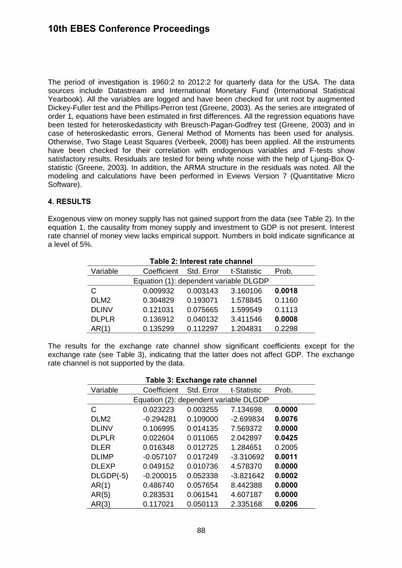
10th EBES Conference Proceedings
88
The period of investigation is 1960:2 to 2012:2 for quarterly data for the USA. The data sources include Datastream and International Monetary Fund (International Statistical Yearbook). All the variables are logged and have been checked for unit root by augmented Dickey-Fuller test and the Phillips-Perron test (Greene, 2003). As the series are integrated of order 1, equations have been estimated in first differences. All the regression equations have been tested for heteroskedasticity with Breusch-Pagan-Godfrey test (Greene, 2003) and in case of heteroskedastic errors, General Method of Moments has been used for analysis. Otherwise, Two Stage Least Squares (Verbeek, 2008) has been applied. All the instruments have been checked for their correlation with endogenous variables and F-tests show satisfactory results. Residuals are tested for being white noise with the help of Ljung-Box Q-statistic (Greene, 2003). In addition, the ARMA structure in the residuals was noted. All the modeling and calculations have been performed in Eviews Version 7 (Quantitative Micro Software). 4. RESULTS Exogenous view on money supply has not gained support from the data (see Table 2). In the equation 1, the causality from money supply and investment to GDP is not present. Interest rate channel of money view lacks empirical support. Numbers in bold indicate significance at a level of 5%.
Table 2: Interest rate channel
Variable Coefficient Std. Error t-Statistic Prob.
Equation (1): dependent variable DLGDP
C 0.009932 0.003143 3.160106 0.0018 DLM2 0.304829 0.193071 1.578845 0.1160
DLINV 0.121031 0.075665 1.599549 0.1113
DLPLR 0.136912 0.040132 3.411546 0.0008 AR(1) 0.135299 0.112297 1.204831 0.2298
The results for the exchange rate channel show significant coefficients except for the exchange rate (see Table 3), indicating that the latter does not affect GDP. The exchange rate channel is not supported by the data.
Table 3: Exchange rate channel Variable Coefficient Std. Error t-Statistic Prob.
Equation (2): dependent variable DLGDP
C 0.023223 0.003255 7.134698 0.0000 DLM2 -0.294281 0.109000 -2.699834 0.0076 DLINV 0.106995 0.014135 7.569372 0.0000 DLPLR 0.022604 0.011065 2.042897 0.0425 DLER 0.016348 0.012725 1.284651 0.2005
DLIMP -0.057107 0.017249 -3.310692 0.0011 DLEXP 0.049152 0.010736 4.578370 0.0000 DLGDP(-5) -0.200015 0.052338 -3.821642 0.0002 AR(1) 0.486740 0.057654 8.442388 0.0000 AR(5) 0.283531 0.061541 4.607187 0.0000 AR(3) 0.117021 0.050113 2.335168 0.0206
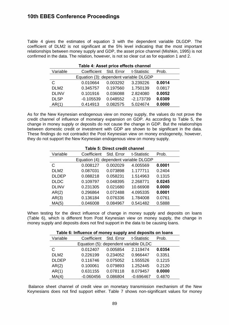
10th EBES Conference Proceedings
89
Table 4 gives the estimates of equation 3 with the dependent variable DLGDP. The coefficient of DLM2 is not significant at the 5% level indicating that the most important relationships between money supply and GDP, the asset price channel (Mishkin, 1995) is not confirmed in the data. The relation, however, is not so clear cut as for equation 1 and 2.
Table 4: Asset price effects channel Variable Coefficient Std. Error t-Statistic Prob.
Equation (3): dependent variable DLGDP
C 0.010664 0.003292 3.239226 0.0014 DLM2 0.345757 0.197560 1.750139 0.0817
DLINV 0.101916 0.036088 2.824080 0.0052 DLSP -0.105539 0.048552 -2.173739 0.0309 AR(1) 0.414913 0.082575 5.024674 0.0000
As for the New Keynesian endogenous view on money supply, the values do not prove the credit channel of influence of monetary expansion on GDP. As according to Table 5, the change in money supply or deposits do not cause the change in GDP. But the relationships between domestic credit or investment with GDP are shown to be significant in the data. These findings do not contradict the Post Keynesian view on money endogeneity, however, they do not support the New Keynesian endogenous view on money supply.
Table 5: Direct credit channel Variable Coefficient Std. Error t-Statistic Prob.
Equation (4): dependent variable DLGDP
C 0.008127 0.002029 4.005569 0.0001 DLM2 0.087031 0.073898 1.177711 0.2404
DLDEP 0.088218 0.058231 1.514963 0.1315
DLDC 0.109797 0.048395 2.268771 0.0245 DLINV 0.231305 0.021680 10.66908 0.0000 AR(2) 0.296864 0.072488 4.095335 0.0001 AR(3) 0.136184 0.076336 1.784008 0.0761
MA(5) 0.046008 0.084967 0.541482 0.5888
When testing for the direct influence of change in money supply and deposits on loans (Table 6), which is different from Post Keynesian view on money supply, the change in money supply and deposits does not find support in the data to be causing loans.
Table 6: Influence of money supply and deposits on loans Variable Coefficient Std. Error t-Statistic Prob.
Equation (5): dependent variable DLDC
C 0.012407 0.005854 2.119474 0.0354 DLM2 0.226199 0.234052 0.966447 0.3351
DLDEP 0.116746 0.075052 1.555526 0.1215
AR(2) 0.100061 0.079893 1.252445 0.2120
AR(1) 0.631155 0.078118 8.079457 0.0000 MA(4) -0.060456 0.086804 -0.696467 0.4870
Balance sheet channel of credit view on monetary transmission mechanism of the New Keynesians does not find support either. Table 7 shows non-significant values for money

10th EBES Conference Proceedings
90
supply and stock prices index. Therefore, no causality runs from money supply to GDP, or from stock prices index to GDP.
Table 7: Balance sheet channel Variable Coefficient Std. Error t-Statistic Prob.
Equation (6): dependent variable DLGDP
C 0.010250 0.003657 2.803151 0.0056 DLM2 0.236366 0.217309 1.087693 0.2781
DLSP -0.122373 0.075537 -1.620039 0.1068
DLDC 0.122766 0.051034 2.405587 0.0171 DLINV 0.121508 0.035904 3.384216 0.0009 AR(1) 0.367315 0.084129 4.366087 0.0000
The most important New Keynesian relationship is represented in Equation 7. Table 8 shows the results of the regression and rejects the New Keynesian theory.
Table 8: Influence of money supply on loans Variable Coefficient Std. Error t-Statistic Prob.
Equation (7): dependent variable DLDC
C 0.007329 0.002984 2.456210 0.0149 DLM2 -0.220638 0.173012 -1.275275 0.2037
DLDC(-1) 0.791065 0.067794 11.66861 0.0000 AR(1) -0.071598 0.092097 -0.777414 0.4379
AR(3) 0.098564 0.079124 1.245700 0.2144
AR(8) -0.205820 0.072642 -2.833324 0.0051
The Post Keynesian view on endogenous money supply has been confirmed to hold in the data. Table 9 and Table 10 show the results of confirmation of the most important Post Keynesian view on loans and reserves (“loans make deposits and deposits make reserves”, as according to Pollin (1991).
Table 9: Relationship from loans to reserves Variable Coefficient Std. Error t-Statistic Prob.
Equation (8): dependent variable DLRES
C 0.065946 0.065268 1.010401 0.3137
DLDC -0.371486 0.137909 -2.693696 0.0077 AR(8) 0.681203 0.138375 4.922872 0.0000 AR(1) 0.180569 0.079264 2.278087 0.0239 MA(12) 0.756342 0.134913 5.606141 0.0000
Table 10: Relationship from loans and deposits to reserves
Variable Coefficient Std. Error t-Statistic Prob.
Equation (9): dependent variable DLRES
C -0.021721 0.014725 -1.475084 0.1420
DLDC -1.077962 0.369385 -2.918259 0.0040 DLDEP 3.132487 0.513970 6.094682 0.0000 AR(1) 0.282862 0.077106 3.668488 0.0003 AR(2) 0.161972 0.083935 1.929727 0.0552
MA(12) 0.198089 0.103441 1.914996 0.0571

10th EBES Conference Proceedings
91
Table 11 confirms that “loans create deposits” and not the other way around, as New Keynesians have put it (Table 6, row 5, column 4)
Table 11: “Loans create deposits” Variable Coefficient Std. Error t-Statistic Prob.
Equation (10): dependent variable DLDEP
C -36.46526 315211.0 -0.000116 0.9999
DLDC 0.179248 0.058761 3.050467 0.0026 AR(2) 0.181978 0.080284 2.266685 0.0246 AR(12) 0.293434 0.213899 1.371836 0.1719
AR(1) 0.144805 0.086744 1.669330 0.0968
AR(4) 0.379755 0.084800 4.478252 0.0000 MA(12) 0.115591 0.304899 0.379113 0.7051
Table 12 also confirmed the theory of the Equation 11 that change in loans influence the change in GDP. The data shows that the change in loans that happened two period in the past will influence the current value of GDP.
Table 12: Relationship from loans to GDP Variable Coefficient Std. Error t-Statistic Prob.
Equation (11): dependent variable DLGDP
C 0.018259 0.005022 3.635426 0.0004 DLDC 0.106759 0.074207 1.438669 0.1519
DLGDP(-1) -0.146172 0.187247 -0.780634 0.4360
DLGDP(-2) 0.032985 0.115043 0.286715 0.7747
DLDC(-2) -0.086885 0.038522 -2.255477 0.0253 DLDC(-1) 0.006364 0.042469 0.149841 0.8811
AR(1) 0.454951 0.191476 2.376023 0.0185 AR(4) 0.239941 0.080462 2.982038 0.0032 MA(11) 0.231542 0.091354 2.534565 0.0121 MA(5) -0.143080 0.098871 -1.447135 0.1496
Table 13 and Table 14 show that there is support for the bidirectional causality from money supply to GDP. GDP lagged one and three periods influences the change in money supply. And money supply lagged one period influences the change in GDP.
Table 13: Causality from GDP to M2 Variable Coefficient Std. Error t-Statistic Prob.
Equation (12): dependent variable DLM2
C 0.001598 0.003687 0.433584 0.6651
DLGDP 0.018024 0.103177 0.174692 0.8615
DLGDP(-3) 0.576517 0.173578 3.321378 0.0011 DLGDP(-1) -0.282243 0.128987 -2.188145 0.0298 DLM2(-1) 0.641826 0.179149 3.582637 0.0004 DLM2(-3) -0.042341 0.299018 -0.141599 0.8875
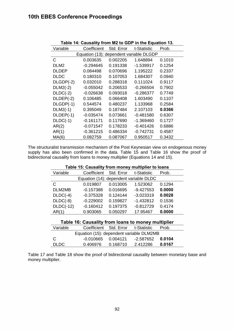
10th EBES Conference Proceedings
92
Table 14: Causality from M2 to GDP in the Equation 13. Variable Coefficient Std. Error t-Statistic Prob.
Equation (13): dependent variable DLGDP
C 0.003635 0.002205 1.648894 0.1010
DLM2 -0.294645 0.191338 -1.539917 0.1254
DLDEP 0.084498 0.070696 1.195222 0.2337
DLDC 0.180310 0.107053 1.684307 0.0940
DLGDP(-2) 0.032010 0.288318 0.111024 0.9117
DLM2(-2) -0.055042 0.206533 -0.266504 0.7902
DLDC(-2) -0.026638 0.093018 -0.286377 0.7749
DLDEP(-2) 0.106485 0.066408 1.603490 0.1107
DLGDP(-1) 0.544574 0.480237 1.133968 0.2584
DLM2(-1) 0.395049 0.187484 2.107103 0.0366 DLDEP(-1) -0.035474 0.073661 -0.481580 0.6307
DLDC(-1) -0.161171 0.117690 -1.369460 0.1727
AR(2) -0.071547 0.178233 -0.401426 0.6886
AR(1) -0.361215 0.486334 -0.742731 0.4587
MA(6) 0.082759 0.087067 0.950517 0.3432
The structuralist transmission mechanism of the Post Keynesian view on endogenous money supply has also been confirmed in the data. Table 15 and Table 16 show the proof of bidirectional causality from loans to money multiplier (Equations 14 and 15).
Table 15: Causality from money multiplier to loans Variable Coefficient Std. Error t-Statistic Prob.
Equation (14): dependent variable DLDC
C 0.019807 0.013005 1.523062 0.1294
DLM2MB -0.157388 0.016695 -9.427553 0.0000 DLDC(-4) -0.375328 0.124144 -3.023319 0.0028 DLDC(-8) -0.229002 0.159827 -1.432812 0.1536
DLDC(-12) -0.160412 0.197375 -0.812729 0.4174
AR(1) 0.903065 0.050297 17.95467 0.0000
Table 16: Causality from loans to money multiplier Variable Coefficient Std. Error t-Statistic Prob.
Equation (15): dependent variable DLM2MB
C -0.010665 0.004121 -2.587652 0.0104 DLDC 0.406976 0.168710 2.412286 0.0167
Table 17 and Table 18 show the proof of bidirectional causality between monetary base and money multiplier.
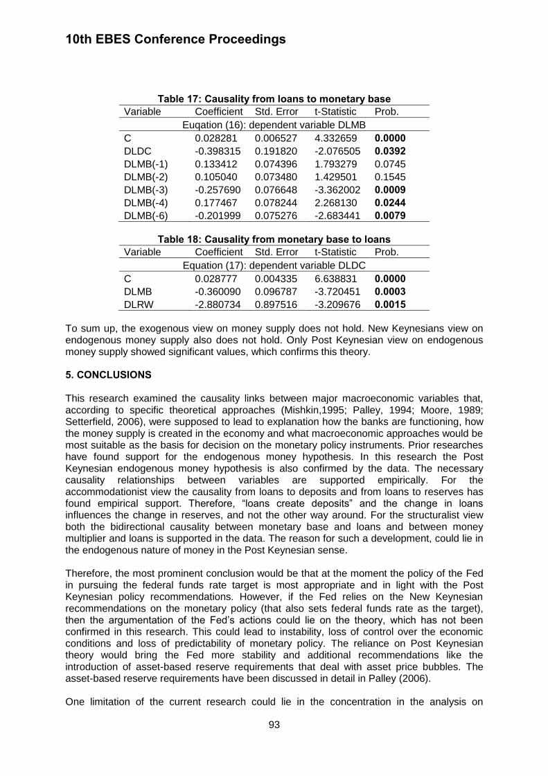
10th EBES Conference Proceedings
93
Table 17: Causality from loans to monetary base Variable Coefficient Std. Error t-Statistic Prob.
Euqation (16): dependent variable DLMB
C 0.028281 0.006527 4.332659 0.0000 DLDC -0.398315 0.191820 -2.076505 0.0392 DLMB(-1) 0.133412 0.074396 1.793279 0.0745
DLMB(-2) 0.105040 0.073480 1.429501 0.1545
DLMB(-3) -0.257690 0.076648 -3.362002 0.0009 DLMB(-4) 0.177467 0.078244 2.268130 0.0244 DLMB(-6) -0.201999 0.075276 -2.683441 0.0079
Table 18: Causality from monetary base to loans
Variable Coefficient Std. Error t-Statistic Prob.
Equation (17): dependent variable DLDC
C 0.028777 0.004335 6.638831 0.0000 DLMB -0.360090 0.096787 -3.720451 0.0003 DLRW -2.880734 0.897516 -3.209676 0.0015
To sum up, the exogenous view on money supply does not hold. New Keynesians view on endogenous money supply also does not hold. Only Post Keynesian view on endogenous money supply showed significant values, which confirms this theory. 5. CONCLUSIONS This research examined the causality links between major macroeconomic variables that, according to specific theoretical approaches (Mishkin,1995; Palley, 1994; Moore, 1989; Setterfield, 2006), were supposed to lead to explanation how the banks are functioning, how the money supply is created in the economy and what macroeconomic approaches would be most suitable as the basis for decision on the monetary policy instruments. Prior researches have found support for the endogenous money hypothesis. In this research the Post Keynesian endogenous money hypothesis is also confirmed by the data. The necessary causality relationships between variables are supported empirically. For the accommodationist view the causality from loans to deposits and from loans to reserves has found empirical support. Therefore, “loans create deposits” and the change in loans influences the change in reserves, and not the other way around. For the structuralist view both the bidirectional causality between monetary base and loans and between money multiplier and loans is supported in the data. The reason for such a development, could lie in the endogenous nature of money in the Post Keynesian sense. Therefore, the most prominent conclusion would be that at the moment the policy of the Fed in pursuing the federal funds rate target is most appropriate and in light with the Post Keynesian policy recommendations. However, if the Fed relies on the New Keynesian recommendations on the monetary policy (that also sets federal funds rate as the target), then the argumentation of the Fed’s actions could lie on the theory, which has not been confirmed in this research. This could lead to instability, loss of control over the economic conditions and loss of predictability of monetary policy. The reliance on Post Keynesian theory would bring the Fed more stability and additional recommendations like the introduction of asset-based reserve requirements that deal with asset price bubbles. The asset-based reserve requirements have been discussed in detail in Palley (2006). One limitation of the current research could lie in the concentration in the analysis on
10th EBES Conference Proceedings
94
contemporaneous causality and, in certain cases, analysis only of this type of causality. This, however, did not become an obstacle in finding the significant relationships. Another limitation could be the closed economy model that has been used for analysis of endogenous money supply view. The extension to an open economy model would be interesting. However, to my best knowledge there is not open economy model for the endogenous money transmission available. In addition, the Two Stage Least Squares and General Method of Moments are used for analysis not taking into account possible cointegrating relations. REFERENCES Alves, A. J., Dymski, G. A. and de Paula, L.-F., 2008. Banking strategy and credit expansion: a post-Keynesian approach. Cambridge Journal of Economics, 32(3), pp.395–420. Angrist, J. and Pischke, J., 2008. Mostly harmless econometrics: An empiricist’s companion. Princeton: Princeton University Press. Arestis, P. and Sawyer, M., 2006. The nature and role of monetary policy when money is endogenous. Cambridge Journal of Economics, 30(6), pp.847–860. Badarudin, Z., Ariff, M. and Khalid, A., 2013. Post-Keynesian money endogeneity evidence in G-7 economies. Journal of International Money and Finance, 33(0), pp.146–162. Bernanke, B. S. and Blinder, A. S., 1992. The federal funds rate and the channels of monetary transmission. The American Economic Review, 82(4), pp.901–921. Bernanke, B. S. and Gertler, M., 1995. Inside the black box: The credit channel of monetary policy transmission. The Journal of Economic Perspectives, 9(4), pp.27–48. Federal Reserve, 2012. 2012 Monetary Policy Releases. [press release] 12 December 2012. Available at: <http://www.federalreserve.gov/newsevents/press/monetary/20121212a.htm> [Accessed 10 May 2013] Granger, C., 1988. Some recent development in a concept of causality. Journal of Econometrics, 39(1–2), pp.199–211. Greene, W.H., 2003. Econometric analysis. 5th ed. New Jersey: Prentice Hall. Hicks, J., 1980. Causality in economics. New York: Basic Books. Howells, P.G., 1995. The demand for endogenous money. Journal of Post Keynesian Economics, 18(1), pp.89-106. Howells, P.G., 1997. The demand for endogenous money: A rejoinder. Journal of Post Keynesian Economics, 19(3), p.429-435. Ireland, P. N., 2005. The monetary transmission mechanism. Boston: Federal Reserve Bank of Boston. [online] Available at: <http://www.bostonfed.org/economic/wp/wp2006/wp0601.pdf> [Accessed 14 April 2013]. Jayaratne, J. and Morgan, D. P., 2000. Capital market frictions and deposit constraints at banks. Journal of Money, Credit, and Banking, 32(1), pp.74–92.
10th EBES Conference Proceedings
95
Kaldor, N., 1970. The new monetarism. Lloyds Bank Review, pp.1–17. King, J., 2002. A history of post Keynesian economics since 1936. Cheltenham: Edward Elgar. Lavoie, M., 2004. The new consensus on monetary policy seen from a post- Keynesian perspective. In: M. Lavoie and M. Seccareccia, eds. 2004. Central banking in the modern world: Alternative perspectives. Cheltenham: Edward Elgar Publishing. Ch. 1. Mackie, J., 1980. The cement of the universe: A study of causation. Oxford: Clarendon Press. Mishkin, F.S., 2004. The economics of money, banking, and financial markets. 7th ed. Boston: Addison Wesley. Mishkin, F.S., 1995. Symposium on the monetary transmission mechanism. The Journal of Economic Perspectives, 9(4), pp.3–10. Moore, B.J., 1998. Accommodation to accommodationism: A note. Journal of Post Keynesian Economics, 21(1), p.175-178. Moore, B.J., 1989. The endogeneity of credit money. Review of Political Economy, 1(1), pp.65-93. Nell, K.S., 2001. The endogenous/exogenous nature of South Africa’s money supply under direct and indirect monetary control measures. Journal of Post Keynesian Economics, 23(2), pp.313–329. Palley, T. I., 1987. Bank lending, discount window borrowing, and the endogenous money supply: A theoretical framework. Journal of Post Keynesian Economics, 10(2), pp.282-303. Palley, T. I., 1994. Competing views of the money supply process: Theory and evidence. Metroeconomica, 45(1), pp.67–88. Palley, T.I., 2003. Asset price bubbles and the case for asset-based reserve requirements. Challenge, 46, pp.53–72. Palley, T.I., 2006. A post keynesian framework for monetary policy: Why interest rate operating procedures are not enough. In: C. Gnos, and L. Rochon, eds. 2006. Post Keynesian principles of economic policy. Cheltenham: Edward Elgar Publishing. Ch. 5. Park, M.-S., 2011. Routes of money endogeneity: A heuristic comparison. Cambridge Journal of Economics, 35(4), pp.685–704. Pearl, J., 2000. Causality: Models, reasoning, and inference. Cambridge: Cambridge University Press. Pollin, R., 1991. Two theories of money supply endogeneity: Some empirical evidence. Journal of Post Keynesian Economics, 13(3), pp.366–396. Schularick, M. and Taylor, A.M., 2012. Credit booms gone bust: Monetary policy, leverage

10th EBES Conference Proceedings
96
cycles, and financial crises, 1870–2008. American Economic Review, 102(2), pp.1029–1061. Shanmugam, B., Nair, M. and Li, O.W., 2003. The endogenous money hypothesis: Empirical evidence from Malaysia (1985-2000). Journal of Post Keynesian Economics, 25(4), pp.599–611. Setterfield, M. ed., 2006. Complexity, endogenous money and macroeconomic theory: Essays in honour of Basil J. Moore. Cheltenham: Edward Elgar Publishing. Tas, B.K.O. and Togay, S., 2012. A direct test of the endogeneity of money: Implications for Gulf Cooperation Council (GCC) countries. Economic Modelling, 29(3), pp.577–585. Verbeek, M., 2008. A guide to modern econometrics. 2nd ed. West Sussex: John Wiley & Sons Ltd. Vymyatnina, Y., 2006. How much control does Bank of Russia have over money supply? Research in International Business and Finance, 20(2), pp.131–144. Walsh, C., 2003. Monetary theory and policy. 2nd ed. Cambridge, Massachusetts: MIT Press. Wold, H., 1954. Causality and econometrics. Econometrica, 22(2), pp.162-177.
10th EBES Conference Proceedings 23 - 25 May, 2013. NIPPON HOTEL, ISTANBUL, TURKEY ISBN: 978-605-64002-1-6. WEBSITE: www.ebesweb.org
97
THE INFLUENCE OF CAPITAL STRUCTURE ON FINANCIAL PERFORMANCE: EVIDENCE FROM ROMANIAN
MANUFACTURING COMPANIES
SORANA VATAVU Finance Department, Faculty of Economics and Business Administration
West University of Timisoara Romania
[email protected] Abstract: This research aims to establish the relationship between capital structure decisions and performance of 196 listed Romanian companies operating in the manufacturing sector, over a period of eight-years (2003-2010). The analysis is based on cross sectional regressions. The capital structure ratios are long-term debt, short-term debt, total debt and total equity, while return on assets and return on equity are the performance proxies. Previous research shows that asset tangibility, tax, risk, liquidity and inflation determine the capital structure in Romanian manufacturing companies, and thus they will be included in the analysis. Results indicate that debt ratios have a negative impact on corporate performance, although long-term debt was not statistically significant, while equity induces a positive effect on the profitability of Romanian manufacturing companies. This research is the first one to examine the relationship between capital structure and financial performance in Romanian listed companies operating in one industry only, which makes its findings more reliable. Keywords: Determinant of Capital Structure, Leverage, Equity, Financial Performance 1. INTRODUCTION Financing decisions is a major decision area in companies because an optimal capital structure referring to the corporate financing mix that maximizes the market share price and the value of the company. Modigliani and Miller (1958) demonstrated the irrelevance of capital structure in firm value, although the assumption is valuable only in perfect market conditions, where all investors have free access to market information, there are zero transaction costs and no tax difference between dividends and capital gains. However, real economies are far from perfect and thus many financing decisions theories were developed over time in order to demonstrate the purpose of capital mix and its role in company value. A few years after the irrelevance theory, Miller and Modigliani (1963) revised the conditions and explained that interest expenses are tax deductible, and therefore firms value increases with higher debt ratios. After them the capital structure literature developed and researchers found many more variables that influence both financing decisions and financial performance. This research tries to identify how debt-equity mix influences firm performance in manufacturing companies listed on the Bucharest Stock Exchange. The study is based on previous research which analyzed the determinants of capital structure in the same manufacturing firms. It was discovered that fixed assets, liquidity, taxation, business risk and annual inflation rate are some of the most influential factors for financing decisions (Vatavu 2012, 2013). Therefore, these factors will be included along with debt and equity ratios, studying their relationships with firm performance.
10th EBES Conference Proceedings
98
2. LITERATURE REVIEW The traditional theory of capital structure strongly believes that the optimal mix of capital ensures a low weighted average cost of capital that maximizes the market value per share. But the leverage and equity ratios are not sufficient in determining performance, because there are multiple factors interfering with these relationships. Akintoye (2009) confirmed the role of business risk, taxes, managerial behavior or financial flexibility in the analysis of firm performance. He explained that since capital structure is based on the trade-off between risk and expected return, these are crucial factors in determining a target capital mix. This target would guide companies towards an ideal mix of debt and equity that minimizes the cost of capital and maximizes the company value. Moreover, any changes made in the level of debt or equity will modify the firm’s value. According to tax benefits it is expected that under the tax burden, companies would borrow more and obtain a higher performance. Some think that performance is the total market value of a firm or the sum between market value of equity and value of equity options (Cole and Mehran 1998, Merz and Yashiv 2007). Others consider that company value refers to more than market capitalization, taking into consideration the value of firm’s operation assets (Mehran 1995, Ang et al. 2000, Allen et al. 2009). Either way, firm performance reflects how effectively companies manage their resources. There is a multitude of capital structure indicators that influence the firm performance and profitability. Previous studies report a positive relationship between short-term debt and total debt and performance in Ghanian or Iranian firms, but a negative impact from long-term debt to profitability, expressed thorugh return on equity (Abor 2005). A negative correlation between leverage and performance, described by the ratio of earnings before interest and tax to total assets, was found in the Chinese firms (Huang and Song 2006, Chakraborty 2010). There are also studies such as Ebaid’s (2009), where no significant impact was found between capital structure choices and performance. Studies analysing the impact of financing decisions on performance and profitability use to employ some of the most relevant capital structure determinants. The Romanian manufacturing companies tend to follow the rule of financing fixed assets with long-term resources and temporary needs with short-term debt. The significant direct relationship between debt and tax proves that tax-saving is not the main reason for borrowing, because manufacturing companies raise their liabilities when they are low on cash. Therefore, by accessing debt with short-term maturity when they are in financial distress, companies increase their business risk. Moreover, there was evidence that companies turn to temporary debt when inflation rate rises (Vatavu 2012, 2013). 3. DATA AND METHODOLOGY 3.1. Sample The sample analyzed includes 196 listed Romanian companies operating in the manufacturing industry. Only one sector was chosen in order to avoid misleading results. Some factors, such as economic risk, vary across the corporate domains, and so they influence the capital structure decisions. These become biased, affecting the corporate performance, which can vary differently across economic sectors. All companies are listed on the Bucharest Stock Exchange. The sample consists in a period of eight years, from 2003 to 2010, and it was gathered from the official website of the Bucharest Stock Exchange.

10th EBES Conference Proceedings
99
3.2. Variables Two performance indicators were chosen as dependent variables. Return on assets (ROA) as net income to total assets, and return on equity (ROE), the ratio of net income to shareholders’ equity. The independent variables are debt ratios, TOTD, LGTD, SHTD - the ratios of total liabilities, long-term liabilities and respectively short-term liabilities to total assets – and the equity ratios, TE – the ratio of total equity to total assets. Only one of these independent variables will be used in the regression models. The determinants of capital structure in Romanian manufacturing companies will perform as control variables in order to explain more of the variance in performance indicators. These variables are asset tangibility (TANG), defined as the ratio of fixed assets to total assets, tax (TAX), described by the ratio of tax to earnings before interest and tax, business risk (BUSRISK), the ratio of standard deviation of earnings before interest and tax to total assets, liquidity (LIQUID), the ratio of current assets to current liabilities, and the annual inflation rate (INFL) provided by Eurostat. 3.3. Empirical model This study tries to discover some of the variables influencing corporate performance on a time series cross-sectional data over the 2003 – 2010 period. ROA and ROE will be regressed on a group of variables, therefore performance can be understood through the following function: Profitability = f(debt, equity, tangibility, tax, business risk, liquidity, inflation) (1) The static linear models used in the analysis are presented in the second and third equations:
ROAit = i + 1CapStrit + 2Tangit + 3Taxit + 4BusRiskit + 5Liquidit + 6Inflit + it (2)
ROEit = i + 1CapStrit + 2Tangit + 3Taxit + 4BusRiskit + 5Liquidit + 6Inflit + it (3)
where i (i = 1…196) is the unknown intercept for every company, t (t=2003..2010)
represents the year analysed, the s are the coefficients for every independent variable and
it is the error term. CapStr refers to the four capital structure ratios previously mentioned. Only one will be used in every regression in order to avoid autocorrelation. Several methods will be used to test the static models considered: Pooled Ordinary Least Squares (OLS), Fixed Effects using least squares dummy variable for companies (LSDV), Fixed Effects with n entity-specific intercepts (FE) and Random Effects (RE). The Hausman test will reveal the better model from the latter two. Finally, in order to correct the issues of heteroskedasticity and autocorrelation a final regression with necessary corrections will be estimated. Fixed effects models explore the relationships between independent variables and regress and in separate entities, assuming in this case that companies have their own characteristics that will influence the relationships between variables. Random effects models imply a random variation across companies, uncorrelated to explanatory variables.

10th EBES Conference Proceedings
100
3.4. Descriptive statistics Table 1 presents the summary statistics of the variables used in the analysis. Mean values contain valuable information because they refer to the majority of the manufacturing companies listed on the Bucharest Stock Exchange.
Table 1: Descriptive statistic data Variable Obs. Mean Std. Dev. Min Max roa 1490 -0.0029618 0.1537931 -1.384159 2.040877
roe 1481 -0.056167 5.551735 -203.3527 25.94096
totd 1485 0.4699652 0.3868654 0.006935 5.023044
lgtd 1387 0.0895043 0.169613 0 1.763594
shtd 1490 0.3850431 0.3504402 0 5.023044
te 1490 0.5253196 0.3807309 -4.070073 1.06655
tang 1490 0.5398824 0.1968779 0.018384 0.999539
tax 1491 0.1777303 0.3823952 0 7.992565
busrisk 1363 0.0948262 0.1156391 0.000207 1.695361
liquid 1489 2.194295 2.848019 0.004776 47.83741
infl 1568 8.275 3.041838 4.9 14.1
The average ratio of ROA and ROE is just above zero, showing that Romanian manufacturing companies have difficulties in registering profits. The mean of total debt ratio is 0.47, while long-term debt shows an average of 0.089 and short-term debt is about 0.38. This indicates that analyzed companies prefer liabilities over short periods of time. More than 12% of long-term debt data is missing and more than 25% of this sample is operating without any long-term liabilities. This might affect the significance of results obtained from regressions using this variable. The average equity ratio is approximately 0.53, indicating that both internal and borrowed funds are used in fixed assets investments. Tangibility ratio is on average 0.54, showing that manufacturing companies try to maintain an equilibrium of fixed and current assets. This means that manufacturing companies either own a low proportion of fixed assets, or they keep a high degree of cash, accounts receivable, inventory and other liquid assets. The second assumption is more appropriate for this case, considering the average liquidity of 2.19 that means that the proportion of current assets is so large that temporary debt only covers half of them. 3.5. Correlations The correlations between variables are presented in Table 2. High correlations can be observed between debt ratios, and between debt and equity ratios, but as long as only one of these variables is included in regressions, there will be no problems with the results returned. The correlations indicate that all three debt ratios have a negative impact on ROA and ROE, while shareholders’ equity is directly related to both performance variables. Additionally, the proportion of fixed assets and business risk are indirectly correlated to the dependent variables. The rest of the control variables, tax, liquidity and inflation, vary in the same direction as performance does.
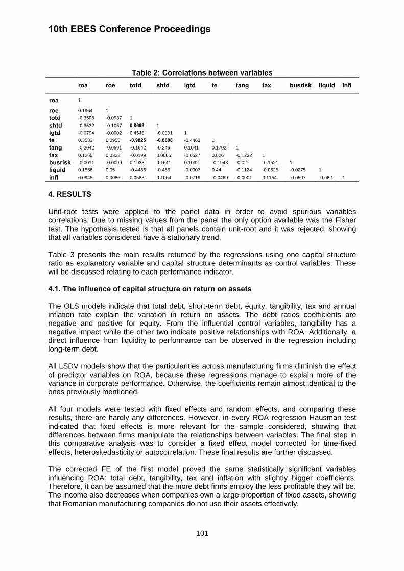
10th EBES Conference Proceedings
101
Table 2: Correlations between variables roa roe totd shtd lgtd te tang tax busrisk liquid infl
roa 1
roe 0.1964 1
totd -0.3508 -0.0937 1
shtd -0.3532 -0.1057 0.8693 1
lgtd -0.0794 -0.0002 0.4545 -0.0301 1
te 0.3583 0.0955 -0.9825 -0.8688 -0.4463 1
tang -0.2042 -0.0591 -0.1642 -0.246 0.1041 0.1702 1
tax 0.1265 0.0328 -0.0199 0.0065 -0.0527 0.026 -0.1232 1
busrisk -0.0011 -0.0099 0.1933 0.1641 0.1032 -0.1943 -0.02 -0.1521 1
liquid 0.1556 0.05 -0.4486 -0.456 -0.0907 0.44 -0.1124 -0.0525 -0.0275 1
infl 0.0945 0.0086 0.0583 0.1064 -0.0719 -0.0469 -0.0901 0.1154 -0.0507 -0.082 1
4. RESULTS Unit-root tests were applied to the panel data in order to avoid spurious variables correlations. Due to missing values from the panel the only option available was the Fisher test. The hypothesis tested is that all panels contain unit-root and it was rejected, showing that all variables considered have a stationary trend. Table 3 presents the main results returned by the regressions using one capital structure ratio as explanatory variable and capital structure determinants as control variables. These will be discussed relating to each performance indicator. 4.1. The influence of capital structure on return on assets The OLS models indicate that total debt, short-term debt, equity, tangibility, tax and annual inflation rate explain the variation in return on assets. The debt ratios coefficients are negative and positive for equity. From the influential control variables, tangibility has a negative impact while the other two indicate positive relationships with ROA. Additionally, a direct influence from liquidity to performance can be observed in the regression including long-term debt. All LSDV models show that the particularities across manufacturing firms diminish the effect of predictor variables on ROA, because these regressions manage to explain more of the variance in corporate performance. Otherwise, the coefficients remain almost identical to the ones previously mentioned. All four models were tested with fixed effects and random effects, and comparing these results, there are hardly any differences. However, in every ROA regression Hausman test indicated that fixed effects is more relevant for the sample considered, showing that differences between firms manipulate the relationships between variables. The final step in this comparative analysis was to consider a fixed effect model corrected for time-fixed effects, heteroskedasticity or autocorrelation. These final results are further discussed. The corrected FE of the first model proved the same statistically significant variables influencing ROA: total debt, tangibility, tax and inflation with slightly bigger coefficients. Therefore, it can be assumed that the more debt firms employ the less profitable they will be. The income also decreases when companies own a large proportion of fixed assets, showing that Romanian manufacturing companies do not use their assets effectively.
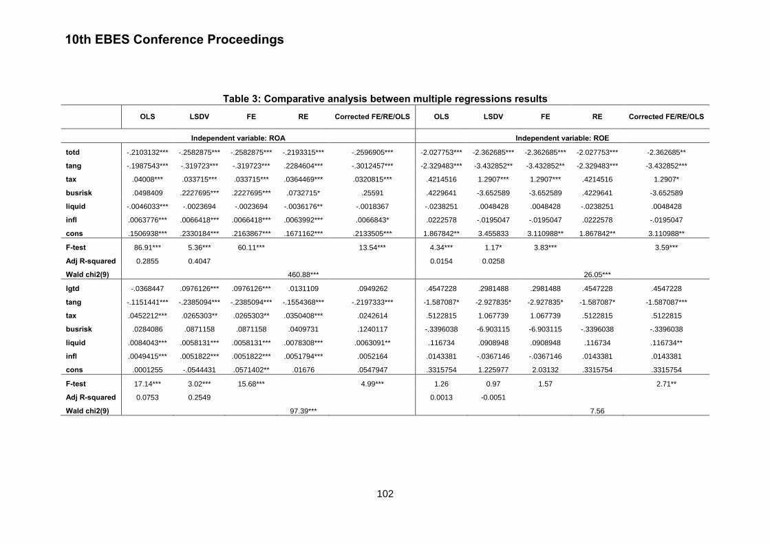
10th EBES Conference Proceedings
102
Table 3: Comparative analysis between multiple regressions results
OLS LSDV FE RE Corrected FE/RE/OLS OLS LSDV FE RE Corrected FE/RE/OLS
Independent variable: ROA Independent variable: ROE
totd -.2103132*** -.2582875*** -.2582875*** -.2193315*** -.2596905*** -2.027753*** -2.362685*** -2.362685*** -2.027753*** -2.362685**
tang -.1987543*** -.319723*** -.319723*** .2284604*** -.3012457*** -2.329483*** -3.432852** -3.432852** -2.329483*** -3.432852***
tax .04008*** .033715*** .033715*** .0364469*** .0320815*** .4214516 1.2907*** 1.2907*** .4214516 1.2907*
busrisk .0498409 .2227695*** .2227695*** .0732715* .25591 .4229641 -3.652589 -3.652589 .4229641 -3.652589
liquid -.0046033*** -.0023694 -.0023694 -.0036176** -.0018367 -.0238251 .0048428 .0048428 -.0238251 .0048428
infl .0063776*** .0066418*** .0066418*** .0063992*** .0066843* .0222578 -.0195047 -.0195047 .0222578 -.0195047
cons .1506938*** .2330184*** .2163867*** .1671162*** .2133505*** 1.867842** 3.455833 3.110988** 1.867842** 3.110988**
F-test 86.91*** 5.36*** 60.11***
13.54*** 4.34*** 1.17* 3.83*** 3.59***
Adj R-squared 0.2855 0.4047
0.0154 0.0258
Wald chi2(9)
460.88***
26.05***
lgtd -.0368447 .0976126*** .0976126*** .0131109 .0949262 .4547228 .2981488 .2981488 .4547228 .4547228
tang -.1151441*** -.2385094*** -.2385094*** -.1554368*** -.2197333*** -1.587087* -2.927835* -2.927835* -1.587087* -1.587087***
tax .0452212*** .0265303** .0265303** .0350408*** .0242614 .5122815 1.067739 1.067739 .5122815 .5122815
busrisk .0284086 .0871158 .0871158 .0409731 .1240117 -.3396038 -6.903115 -6.903115 -.3396038 -.3396038
liquid .0084043*** .0058131*** .0058131*** .0078308*** .0063091** .116734 .0908948 .0908948 .116734 .116734**
infl .0049415*** .0051822*** .0051822*** .0051794*** .0052164 .0143381 -.0367146 -.0367146 .0143381 .0143381
cons .0001255 -.0544431 .0571402** .01676 .0547947 .3315754 1.225977 2.03132 .3315754 .3315754
F-test 17.14*** 3.02*** 15.68***
4.99*** 1.26 0.97 1.57 2.71**
Adj R-squared 0.0753 0.2549
0.0013 -0.0051
Wald chi2(9)
97.39***
7.56
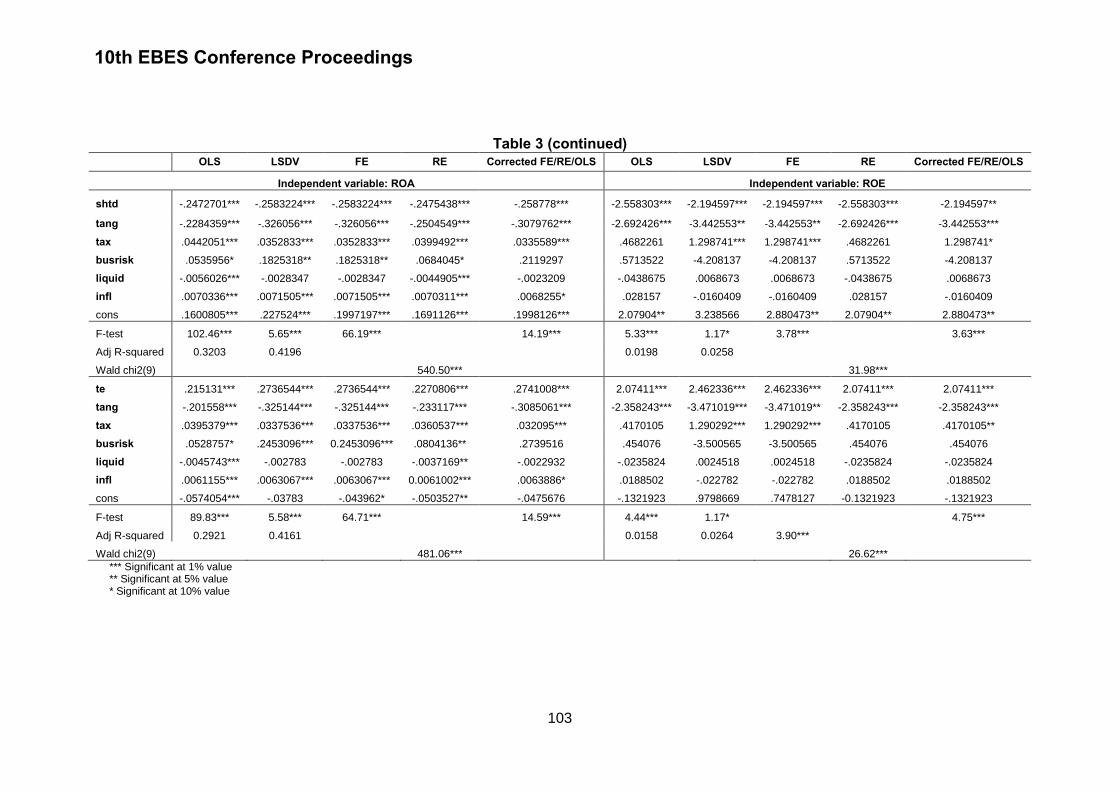
10th EBES Conference Proceedings
103
Table 3 (continued)
OLS LSDV FE RE Corrected FE/RE/OLS OLS LSDV FE RE Corrected FE/RE/OLS
Independent variable: ROA Independent variable: ROE
shtd -.2472701*** -.2583224*** -.2583224*** -.2475438*** -.258778*** -2.558303*** -2.194597*** -2.194597*** -2.558303*** -2.194597**
tang -.2284359*** -.326056*** -.326056*** -.2504549*** -.3079762*** -2.692426*** -3.442553** -3.442553** -2.692426*** -3.442553***
tax .0442051*** .0352833*** .0352833*** .0399492*** .0335589*** .4682261 1.298741*** 1.298741*** .4682261 1.298741*
busrisk .0535956* .1825318** .1825318** .0684045* .2119297 .5713522 -4.208137 -4.208137 .5713522 -4.208137
liquid -.0056026*** -.0028347 -.0028347 -.0044905*** -.0023209 -.0438675 .0068673 .0068673 -.0438675 .0068673
infl .0070336*** .0071505*** .0071505*** .0070311*** .0068255* .028157 -.0160409 -.0160409 .028157 -.0160409
cons .1600805*** .227524*** .1997197*** .1691126*** .1998126*** 2.07904** 3.238566 2.880473** 2.07904** 2.880473**
F-test 102.46*** 5.65*** 66.19***
14.19*** 5.33*** 1.17* 3.78*** 3.63***
Adj R-squared 0.3203 0.4196
0.0198 0.0258
Wald chi2(9)
540.50***
31.98***
te .215131*** .2736544*** .2736544*** .2270806*** .2741008*** 2.07411*** 2.462336*** 2.462336*** 2.07411*** 2.07411***
tang -.201558*** -.325144*** -.325144*** -.233117*** -.3085061*** -2.358243*** -3.471019*** -3.471019** -2.358243*** -2.358243***
tax .0395379*** .0337536*** .0337536*** .0360537*** .032095*** .4170105 1.290292*** 1.290292*** .4170105 .4170105**
busrisk .0528757* .2453096*** 0.2453096*** .0804136** .2739516 .454076 -3.500565 -3.500565 .454076 .454076
liquid -.0045743*** -.002783 -.002783 -.0037169** -.0022932 -.0235824 .0024518 .0024518 -.0235824 -.0235824
infl .0061155*** .0063067*** .0063067*** 0.0061002*** .0063886* .0188502 -.022782 -.022782 .0188502 .0188502
cons -.0574054*** -.03783 -.043962* -.0503527** -.0475676 -.1321923 .9798669 .7478127 -0.1321923 -.1321923
F-test 89.83*** 5.58*** 64.71***
14.59*** 4.44*** 1.17* 4.75***
Adj R-squared 0.2921 0.4161
0.0158 0.0264 3.90***
Wald chi2(9)
481.06***
26.62***
*** Significant at 1% value ** Significant at 5% value * Significant at 10% value
10th EBES Conference Proceedings
104
The direct impact taxes have on ROA indicates that companies are more profitable when facing the tax burden, probably because they are more careful in allocating their funds. Similarly, an increased inflation rate makes Romanian manufacturing companies more profitable in terms of their total assets. However, this can also mean that during times of high inflation firms divest their assets. From the second model including long-term debt as a regressor, the corrected fixed effects equation returns a significant negative coefficient for tangibility and a positive one for liquidity. Therefore, Romanian companies perform better when they own less tangible assets. This assumption is confirmed by the liquidity coefficient showing that current assets offer opportunities for more profits. After using the corrected fixed effects model, the short-term debt maintains its negative impact on the return on assets indicator along with the proxies of tangible assets, tax and inflation, which remain statistically significant. In conclusion, firms from manufacturing industry are more profitable in terms of assets when they owe less on a temporary basis. From the control variables it is shown that return on assets is influenced by tangibility indirectly and positively by tax and inflation. These are the some relationships identified in the previous model considering total debt as one of the independent variables. The consistent results were expected as long as most of the listed companies analysed owe a very small proportion of long-term debt, sometimes choosing only temporary liabilities. The corrected fixed effects regression using equity to total assets ratio determines the return on assets through equity, tangibility, tax and inflation. Tangibility is the only variable conducting a negative effect on the assets profitability. The rest of the variables have a direct impact. It can be said that companies are more profitable when they invest less in tangible assets and they maintain a high proportion of equity in their capital structure. Besides, whenever taxes or inflation are up, the return on assets is higher. Evaluating the overall significance of the model, all regressions are relevant, but the best to describe the impact on return on assets is a fixed effects model corrected for heteroskedasticity, autocorrelation and time fixed effects, which reveals the highest coefficients with their previously mentioned direction. 4.2. The influence of capital structure on return on equity In relation to return on equity, from the models referring to debt ratios, only total debt, short-term debt and tangibility show a statistically significant impact. Debt ratios and tangibility maintain their negative coefficients, significant in all models: least square dummy variable, fixed effects, random effects. On the contrary, equity has a positive impact on ROE. Along with total debt, short-term debt and total equity, tax was also found statistically significant for the variance of ROE, but not in all regressions. Although all the comparative regressions were used (OLS, LSDV, FE, RE), the goodness of fit indicated other variables should be selected in order to discover what conducts the variation in return on equity ratio. Finally, the most appropriate method from all is OLS, corrected in order to fulfill all regression assumptions. Based on the results mentioned, the more debt companies use and the more tangible assets they own, the less efficient they are regarding their shareholders’ money. From these relationships, it can be assumed that profits are affected by a high degree of leverage and companies purchase fixed assets with internal funding. On the other side, it can also be assumed that investors are attracted by companies with investment opportunities and thus
10th EBES Conference Proceedings
105
firms acquiring more fixed assets will raise more equity. A direct impact of tax on ROE means that whenever taxes raise, shareholders are reluctant to buy shares and so the proportion of equity in Romanian manufacturing companies decreases. In the model containing long-term debt, two variables were found statistically significant: tangibility, with a negative impact, and liquidity with positive effect on ROE. In other words, the firms return more on shareholders’ investments when liquid assets exceed tangible ones. For the model trying to explain how Romanian manufacturing companies can return more on the ownership interest of stock holders with the use of equity ratio and control variables, results are consistent with the previous findings: shareholders’ equity has a positive impact, while fixed assets have an opposite effect on the dependent variable. Additionally, the corrected OLS model also returns tax as statistically significant. When taxes are high, manufacturing companies tend to invest less in order to retain their earnings. Another assumption would be that under the tax incidence, firms have lower profits and thus they are trying to raise more capital by attracting new investors. 5. CONCLUSIONS Over the 2003-2010 period, the most profitable manufacturing companies were those that maintained a high proportion of equity in their capital structure, avoiding borrowed funds. Shareholders’ equity has a positive impact on performance indicators. On the contrary, total debt and short-term debt have negative relationships with ROA and ROE, while long-term debt shows coefficients with fluctuating signs. Results for regressions including debt with long maturities are not always significant and consistent because a large part of this data is missing. Another significant variable was tangibility: companies owning a large proportion of fixed assets registered lower earnings. Considering that manufacturing sector assumes valuable investments and continuous development, a direct relationship between tangibility and performance would be expected. Results however indicate that in Romania, manufacturing companies either do not use their assets effectively or they do not have sufficient internal funding to undertake profitable investments. Data provides information that companies barely use debt with long maturities. Moreover, sometimes they operate without long-term debt over a few years. Therefore, the decision of accessing borrowed funds for their growth opportunities would be an exceptional one. Taxes have a direct impact on performance indicators. Although higher taxation is expected to affect the net income, it seems that Romanian companies are more profitable when facing the tax burden, probably because they allocate their funds more effectively. Similarly, inflation has a positive impact on ROA. Although this means that high profits are related to increased inflation rates, it is be more logic to consider that during times of high inflation Romanian firms divest their assets. And this would also prove the negative relationship between tangible assets and performance: because of high inflation companies drop some of their fixed assets, consequently some costs, and become more profitable. Taxes can greatly affect the relationship between equity and performance. Results showed that high taxation makes companies with larger equity ratios and limited fixed assets more profitable. This could mean that Romanian manufacturing companies are not eager to grow: they do not use their internal funding, nor do they access debt for future investments. However, debt is used when companies are in financial difficulties, they face high business risk, and they cannot settle due to their lack of cash.
10th EBES Conference Proceedings
106
Future research should be conducted in order to find variables that better describe the variation in return on equity, and other performance indicators should be included in the analysis for a better understanding of how capital structure and financing decisions influence the financial performance of Romanian companies. REFERENCES Abor, J., 2005. The effect of capital structure on profitability: An empirical analysis of listed firms in Ghana. The Journal of Risk Finance, 6(5), pp.438-447. Akintoye, I.R., 2009. Sensitivity of performance to capital structure. Banking and Finance Letters, 1(1), pp.29-35. Allen, F., Carletti, E. and Marquez, R.S., 2009. Stakeholders capitalism, corporate governance and firm value. Wharton Financial Institutions Center Working Paper, 09-28. Ang, J.S., Cole, R.A. and Lin, J.W., 2000. Agency costs and ownership structure. The Journal of Finance, 55(1), pp.81-106. Chakraborty, I., 2010. Capital structure in an emerging stock market: The case of India, Research in International Business and Finance, 24(3), pp.295-314. Cole, R.A. and Mehran, H., 1998. The effect of changes in ownership structure on performance: Evidence from the thrift industry. Journal of Financial Economics, 50(3), pp.291-317. Ebaid, E.I., 2009. The impact of capital structure choice on firm performance: Empirical evidence from Egypt. The Journal of Risk Finance, 10(5), pp.477-487. Huang, S., and Song, F., 2006. The determinants of capital structure: Evidence from China. China Economic Review, 17(1), pp.14-36. Mehran, H., 1995. Executive compensation structure, ownership, and firm performance. Journal of Financial Economics, 38(2), pp.163-184. Modigliani, F. and Miller, M.H., 1958. The cost of capital, corporation finance and the theory of investment. American Economic Review, 48(3), pp.261–297. Modigliani, F. and Miller, M., 1963. Corporate income taxes and the cost of capital: A correction. American Economic Review, 53(3), pp.433–443. Merz, M. and Yashiv, E., 2007. Labor and the market value of the firm. American Economic Review, American Economic Association, 97(4), pp.1419-1431. Vatavu, S., 2012. Determinants of capital structure: Evidence from Romanian manufacturing companies. 1st Advanced Research in Scientific Areas Conference, [online] Available at: <www.arsa-conf.com/archive/?q=2012-ARSA-7::pdf::2:8> [Accessed 13 January 2013]. Vatavu, S., 2013. The capital structure determinants using comparative analysis: Evidence from manufacturing companies listed on the Bucharest Stock Exchange. In: University of the West Timisoara, Faculty of Economics and Business Administration, The International

10th EBES Conference Proceedings
107
Conference “Current Economic Trends in Emerging and Developing Countries”. Timisoara, Romania, 6-8 June 2013.
10th EBES Conference Proceedings 23 - 25 May, 2013. NIPPON HOTEL, ISTANBUL, TURKEY ISBN: 978-605-64002-1-6. WEBSITE: www.ebesweb.org
108
THE INTEGRATION AND CONCENTRATION/SPECIALIZATION OF EUROPEAN
COUNTRIES ACROSS MANUFACTURING INDUSTRIES
SEYIT KOSE Department of Economics
Abant Izzet Baysal University Turkey
AYKUT SARKGUNESI Department of Management and Organization Administration
Bulent Ecevit University Turkey
[email protected] Abstract: This paper empirically investigates whether the recent European integration
process has significantly affected the concentration/specialization of European countries in fewer numbers of manufacturing industries, or vice versa. Pertaining to scarce empirical work on the issue, there are conflicting arguments but not common agreement about this matter yet. In this regard, we specify an empirical model describing the case benefiting from P. Krugman (1991) and other empirical studies. Employing a balanced panel data set that covers 22 European countries and 23 manufacturing industries for the period 1995-2008, we estimate in general two different regression models, a panel model and country by country estimates from the time series. Findings reveal that overall direct indicators of the integration have had significant impact on the dispersion of the industries in European countries, while some other factors have significantly induced the countries to concentrate/specialize in fewer numbers of industries. On the other hand, due purely to some of the measured integration and other indicators contained in the model, we observe a definite industrial concentration only in 3 countries and a definite industrial diversification only in 2 countries of Europe. The integration indicators and other determinants have affected the industrial distribution differently across the countries. Keywords: European Integration, Industrial Concentration, Industrial Specialization, Regional Clusters
1. INTRODUCTION Long-run disturbing disparities in various social and economic factors across nations and regions have urged academicians and politicians to focus on the issue more broadly and deeply in recent decades. Previous neo-classical theory (Solow, 1956) has not come up well with the current observed phenomenon and the findings of some recent empirical studies on which. The earlier empirical studies in the main stream tradition have found some evidence of convergence, which were weak or frequently conditional (Barro and Sala-i-Martin, 1992; Mankiw et al. 1992; Islam, 1995), whereas the other studies particularly the ones in different approaches could not observe any convergence or even observed a divergence across spatial economic units (Quah, 1990 and 1996; Canova and Marcet, 1995; Pritchett, 1997; Desdoigts, 1999; Hall and Jones, 1999; Royo, 2010). On the other hand, the latest studies have observed an economic convergence of the developing and emerging countries towards the developed ones after the beginning of 1990s in the stronger globalization era, but a
10th EBES Conference Proceedings
109
substantial divergence between the two groups of countries prior to that following the industrial revolution (Rodrick, 2011; Allen, 2012; Dervis, 2012). However, beyond very few numbers of those catching up countries in recent two decades, a majority of less developed countries have remained lagging behind. Thus, most of the recent observations and the findings of empirical studies in different approaches have displayed that the economic gaps across geographical units in major part have not declined, on the contrary increased in some cases. Production factors, various production industries and other economic activities, and population have concentrated in certain countries and regions. In this regard, after some economists spelled out some alternative arguments and approaches to the neo-classical theory and its predictions at the beginning, in order to build sound alternative theoretical models they had to put forward three presumptions, which are (i) heterogeneous of spatial units in many aspects, (ii) positive externalities from concentration of economic activities in location, hence non-decreasing marginal returns to production factors and increasing returns to scales in production and (iii) usually non-perfect competition situations in the markets. These three presumptions have provided a basis for developing different models of explaining the currently observed cross-section disparities (Fujita and Thisse, 2009). In this path, various types of endogenous growth models that built in the main stream tradition could predict even divergence in economic variables across spatial economic units and over time in a spatial economy (Lucas, 1988 and 1990; Romer, 1986 and 1990; Howitt, 2000). Moreover, some theoretical models and empirical studies have dealt with and investigated the observed economic disparities across spatial units in different strands; prevalent ones of which are at the one hand “New Institutionalism Approach” attributed primarily to D. C. North (1990) and at the other hand “New Economic Geography” attributed primarily to P. Krugman (1991). Furthermore, the findings and observations of various empirical studies on whether the globalization and various types of regional integrations of cross-countries have increased the concentration of economic activities or on the contrary they have led to the dispersion of those across countries and regions are disputed and inconclusive matter yet. Likewise, the European countries have experienced a rapidly deepening and widening integration process particularly in recent two decades. Some studies have investigated the issue, but most of them are theoretical modeling and simulations of them; empirical studies with real-life data are still very scarce and do not test sufficiently the impacts of all the integration indicators together on the concentration of economic activities across European geography. Socio-economic development disparities across European Union (EU) countries and regions have expanded further in particular following the enlargement of the integration towards Central and East European (CEE) countries since 1994. EU has allocated almost one-third of its budget into the socio-economic policies in order to harmonize the policies and institutions, and to diminish the structural dissatisfying distinctions across the member or potential member countries and the regions. Main objective from that is to shift industrial locations toward peripheral regions as well, rather than directly redistribution of income more equally across countries and regions (Pflüger and Südekom 2007). Sala-i-Martin (1996) found a slow convergence across EU regions between the years 1950-1990, but in the following years he observed that the cross-regional divergence has getting become stronger especially as the integration has progressed more. According to Amiti (1999), clusters of economic activities have multiplied in all EU countries over the further integration years. All of these developments display that the European regional integration process and the clusters of industries, employment and incomes are vital issues in the EU agenda (Ottaviano and Thisse, 2002). EU Commission emphasizes the European Common Market (European Economic Union) and European Monetary Union (EMU) as vital policy tools in order to
10th EBES Conference Proceedings
110
moderate the dissatisfying socio-economic differences as a priority aim among the others (EU Commission, 2012). Therefore, this article investigates whether the recent European integration process has significantly affected the distribution of manufacturing industries over the European geography. It tries to explain whether the integration has resulted in the manufacturing industries to concentrate in certain European countries and led to the specialization of the countries in certain activities further, or vice versa. In this regard, we adopt an approach in the version of P. Krugman (1991) and adapt it to develop an empirical model in order to describe our case in this study as well as benefiting from other empirical studies. By exploiting panel data regression techniques, we test whether the variables representing the European integration process have significant impact on the distribution of economic activities, and determine which way and to what extent they have influenced them. We could come up with a balanced panel data set that covers 22 European countries and 23 manufacturing industries (ISIC Rev-3) for the period 1995-2008, which are the best available accompanied data for all the required variables in order to test the argument of this study. We first calculate a particular concentration (specialization) index of the manufacturing industries for the European countries. Next, we exploit some proxy indicators for the European integration process as explanatory variables of the developments in the concentration index. Following the theoretical and empirical studies of P. Krugman and the others, we assume that the European integration implies further mobility of commercial products, production factors, people, ideas, technical-knowledge and technology. Beside a few others, we use total gross domestic products (GDP) of countries for controlling their home market (economic size) effects and a distance variable to the core-market for controlling the transportation costs of the countries in Europe, as well. On the other hand, Turkey signed the Customs Union agreement with EU at the end of 1995 and it has been a candidate country that has been compromising to qualify towards the membership since 2004. So, the EU integration has influenced the developments in the Turkish economy as well, as it has already taken place within the integration process. Therefore, it is also considerable piece of knowledge for Turkey to determine what factors of the European integration process, how to and which way, have affected the distribution of manufacturing industries among the countries. The results of this work will also shed some light on the question whether the European integration will cause the manufacturing industries to cluster in the core European countries in order to benefit from agglomeration economies or on the contrary to disperse towards the peripheral European countries in order to benefit from the advantages of factor (particularly labor) costs and the costs of transportation to the countries out of Europe so as to improve their international competition powers. Thereby, we will predict whether labor and population will migrate further from the periphery towards the core or vice versa, as well. We exploit the data set and the defined variables in order to estimate in general two different regression models. First, by combining the information from both cross-countries and over-time, we estimate a panel model in order to acquire findings of comparing the cross-countries and of representative for all Europe. Next, European countries are heterogeneous in many specific characteristics, so it is quite plausible they have different trajectories of concentration or diversification in manufacturing industries. Therefore, we examine the impacts of the integration indicators on the industrial concentration (specialization) of the countries one by one over their time series data, in addition to the overall investigation through the panel data method.
10th EBES Conference Proceedings
111
The findings overall reveal that the direct integration factors beside the home market effects have significantly declined the concentration of European countries in fewer number of manufacturing industries, whereas some other factors have significantly increased the concentration and specialization of the countries in certain industries during the period 1995-2008. On the other hand, due to solely some of the measured integration indicators and measured other factors contained in the model, we have observed a definite industrial concentration only in 3 countries (Denmark, Finland and Ireland) and a definite industrial diversification only in 2 countries (Italy and Sweden) of Europe. The integration indicators and other determinants have affected the distribution of the industries differently across the European countries. This paper provides a summary of the related literature in the next section 2; sources of the data, definitions of the variables and specification of the empirical model follow that in section 3; estimations and analyses of the findings are submitted in section 4; and the conclusions are discussed in final section 5. 2. DATA, VARIABLES AND EMPIRICAL MODEL SPECIFICATION This article investigates whether the recent European integration process has significantly affected the distribution of manufacturing industries in European countries. It tries to explain whether the integration has significantly resulted in certain industries to concentrate in certain countries and hence led to the specialization of them in certain industries further; or in contrary to that it has led to the industries to diversify more equally in the countries. It also tries to explain what indicators of the integration and at which direction have had considerable impacts on the distribution. In this regard, we adopt an approach in the version of P. Krugman (1991) and adapt it to develop an empirical model in order to explain our case in this study, as well as benefiting from other empirical contributions. First, by exploiting panel data regression techniques, we test whether the variables representing the integration process have had significant impacts on the industrial distribution, and determine which way and to what extent they have influenced that. Next, we examine the impacts of the integration indicators on the industrial concentration (specialization) of the countries one by one over their time series data, in addition to the overall investigation over the panel data. We could come up with the balanced panel data set that cover the 22 European countries and 23 manufacturing industries (ISIC Rev-3) for the period 1995-2008, which are the best available accompanied data for all the required variables in order to test the argument of this study. The sample of countries consists of 20 EU members, Norway and Turkey. The names of countries and manufacturing industries are provided in Appendix A (Tables A1 and A2). Employment and the other data sets are collected from the web sources of respectively International Labor Organization (ILO) and World Bank (WB), which are defined in Appendix A (Table A3). Fujita (2010) has adopted international economic geography models in different category, and many studies have exploited cross-country data as regional units in economic geography literature so far. We first employ a particular index to calculate concentration (specialization) of the manufacturing industries across the European countries for each country and for each year in the period. Applied studies have used various types of indexes in this context with their different both pros and handicaps. We employ a type of Gini Coefficient (Gr,t) that adapted by Ellision and Glaeser (1997), which has been exploited in the
following various works at the same version or at the altered types. This indicator measures the concentration (specialization) as it gets closer to “1” or the dispersion (diversity) of the
10th EBES Conference Proceedings
112
industries as it gets closer to “0” within a country relative to that of the rest. Because we use cross-country data Gini coefficients are so small, so considering their more clear visibility we multiply them by 100 as in the independent variables used in their percentage rates. Next, following the theoretical and empirical studies of P. Krugman and the others, we assume that the European integration implies further mobility of commercial products, production factors, people, ideas, technical-knowledge and technology. Likewise, we exploit some proxy indicators for the European integration process beside a few of others as explanatory variables of the developments in the concentration index. Some of the selected variables are assumed to be direct indicators of the integration while others are assumed to be indirect indicators of that. EU Commission (2012) expresses European common market and EMU as the main policy tools of an integrated Europe. European common market includes not only free movement of goods, but also involves free movement of production factors and EMU. As direct indicators of the integration we employ percentage ratio of national external trade volume to national gross domestic product (GDP) (TRADEr,t) as mobility of products and percentage ratio of national net private foreign capital inflows to national GDP as mobility of capital across the countries (CAPITALr,t). Transaction costs could have substantial impacts on the distribution
of clusters across regions. High transaction costs could cause the regional decomposition of economic activities while low transaction costs could result in clustering of economic activities in certain locations (Combes and Overman, 2003). High transaction costs such as barriers to the mobility with high tariffs or with non-tariff types of implementations, and high transportation costs have led firms of countries to produce for their domestic demands in major part rather than for international common markets (Helble et al. 2007). However,
regional integrations have made easier of firms to produce much more for international markets by reducing transaction costs (Reynolds, 1997). So, we employ a factor of distance to the core-market (LnDISTANCEr) in our model so as to control the cross-country transportation costs in Europe. Considering other transaction costs we include the dummy variables of European Monetary Union (EMUr,t) and of Central and East Europe (CEEr) in the model. As EMU indicates more deepening of the integration, CEE represents more widening of the integration towards new members in CEE. It is likely that both groups of countries could be affected from the integration process differently. Thereby, the variables of TRADEr,t, CAPITALr,t, EMUr,t and CEEr can be assumed to be direct indicators of the integration. According to P. Krugman (1991), one of the crucial factors that cause regional clustering of economic activities is the market size of the domestic local economy so called “home market effect”. Firms tend to cluster closer to big markets in order to benefit from scale economies. Hence, firms that respond to larger domestic demands before the integration could more easily compete in international markets as exporters after the integration. Country that has greater domestic demand could compete as an exporter in the international market and the relevant industries could cluster in which. Thereby, we use natural logarithms of GDP`s of countries (LnGDPr,t) in order to control for their home market (size) effects in the model.
Ottoviano and Thisse (2002) emphasize that mobility of labor force increases as its education level increases. A main reason for which is that developments in the education and skill levels make easier the educated and skilled labor force to look for new jobs in different locations and to move to different locations and social environments for new lives and to transmit their human capitals into there. Other main reason is that the cross-regional wage disparities that are much sharper most probably for more educated and skilled labor force rather than for the less educated labor force, which motivate further the mobility of more educated labor force across regions. Hence, we can assume that more educated
10th EBES Conference Proceedings
113
people can accelerate the integration process so that countries with more educated people can benefit further from the integration process through more mobility of their population both across regions within a country more likely or across countries less likely. So, as the integration progresses, a country with more educated labor force is more probably open to clustering of economic activities in certain locations, ceteris paribus. In addition, the
existence of and accessibility to educated and skilled labor force in the location is accepted as a vital factor for clustering of economic activities in there in many theoretical and empirical studies. Thereby, we contain percentage rate of country population with higher education degree in the population (HIGHEREDUr,t) in our model as an explanatory proxy for an
indirect indicator of the integration. We exploited the higher education indicator because when the other education stages are considered there are not big variations across European countries. Likewise, as an indicator of high-quality of production, accumulated-knowledge and technology level, the percentage ratio of high-tech product exports to national exports (HIGHTECHr,t) is employed in the model. Many theoretical and empirical studies show that
high-tech production activities are highly concentrated in specific locations. In addition, we assume a time deterministic trend that assigns a number to each year starting from 1 for year 1995 until 14 for year 2008 (TIMEt). It is included to capture stable proportionate increases in
the Gini index over time. Definitions and descriptive statistics of the variables are provided in the appendix (Tables A3 and B1). Therefore, we define in general two different regression models in order to estimate and test the impacts of the integration indicators on the industrial distributions of European countries by employing the data set and the variables defined above. First, we specify the following multivariate process of general empirical model, which is linear in its parameters, considering the panel data techniques; Gr,t = α + β1*LnGDPr,t + β2*TRADEr,t + β3*CAPITALr,t + β4*HIGHEREDUr,t + β5*HIGHTECHr,t + β6*LnDISTANCEr + β7*EMUr,t + β8*CEEr + β9*TIMEt + φr + ψt + Ԑr,t (1)
where local coefficient of Gini index (0 < Gr,t < 1) for country r (r = 1, 2, ..., 22) and year t (t =
1995, 1996, ..., 2008) is calculated as
Gr,t
(2)
Li,r = total employment of industry i (i = 1, 2, ..., 23) in country r Li = total employment of industry i in the 22 European countries Lr = total employment in country r L = total employment in the 22 European countries.
α is intercept parameter and β`s are slope parameters of the considered variables. φr implies possible country-specific effects and ψt implies possible time-specific effects. We decide to
estimate the model with the most proper method after testing those effects and certain other concerns by a procedure of model selection tests. At last, we may assume the residual-error terms across countries and years (Ԑr,t) are distributed randomly with mean zero and known
statistical characteristics. Next, the time series form is specified by dropping the time invariant variables and EMU dummy from the panel model above for the country by country estimates as follows;

10th EBES Conference Proceedings
114
(3) Gt = δ + ϴ1*LnGDPt + ϴ2*TRADEt + ϴ3*CAPITALt + ϴ4*HIGHEREDUt + ϴ5*HIGHTECHt + ϴ9*TIMEt + ɳt
where the variables are as defined above but only in their time varying forms. δ is intercept parameter and ϴ`s are slope parameters of the considered variables. The error terms over the years (ɳt) are distributed randomly with mean zero and known statistical characteristics.
3. REGRESSION ESTIMATIONS AND ANALYSES OF EMPIRICAL FINDINGS We first check common unit roots of the variables and then try to determine the most suitable estimation method by a model selection procedure based on the panel data. Following that, we analyze the empirical findings from the panel data estimates. Next, we analyze the results from the country by country time series estimates. An agreement does not exist on the issue in the literature yet, so it is still an unsolved empirical matter; and hence before reaching sound empirical findings, we do not want to speculate on the directions and the sizes of the impacts of the integration and other variables on the industrial distribution in European countries. 3.1. Results from panel data estimation procedure In order to avoid spurious regression, the unit roots of the relevant variables are searched first. With regard to Levin, Lin & Chu common unit root test, all the variables are found to be statistically stationary at 1% level but only one at 5% level of significance when the form with individual intercept and trend is chosen (Table 1). In addition, following Westerlund (2007) we have checked the co-integrations between the dependent variable and the independent variables one by one; and found significant co-integrations for all the variables with regard to at least two statistics but for CAPITALr,t with regard to one statistic at 5% level or less (see
Appendix B, Table B2).
Table 1: Levin, Lin & Chu common unit root tests (N=308 with CS=22 & TS=14)
Variables Ho: Common unit root process
Individual Intercept Individual Intercept and Trend t-statistic Prob. t-statistic Prob.
Gr,t -2.460** 0.0070 -3.644** 0.0001
LnGDPr,t 10.240 1.0000 -3.910** 0.0000
TRADEr,t -2.339** 0.0097 -4.654** 0.0000
CAPITALr,t -5.451** 0.0000 -6.671** 0.0000
HIGHEREDUr,t 0.726 0.7660 -6.436** 0.0000
HIGHTECHr,t -3.154** 0.0008 -2.143* 0.0161
Note: (**) and (*) indicate significance levels respectively at 1% and 5%.
Next, in order to decide the most proper estimation method we follow a procedure of model selection tests in Table 2. Unit effects and time effects are jointly and separately tested by using a likelihood ratio test (see Baltagi, 2005). We have found only statistically significant cross-section effects, but not period effects at 1% or 5% levels of significance. According to Hausman Test, we could not reject the null hypothesis that the existing cross-section effects are random at 5% level of significance. Hence, we come up with an estimation method of the panel model with one-way cross-section random effects, which is a consistent and more efficient estimator (see Wooldridge, 2002).
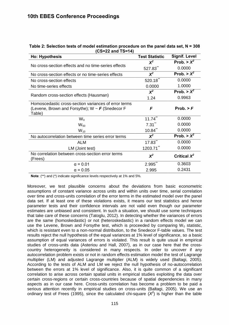
10th EBES Conference Proceedings
115
Table 2: Selection tests of model estimation procedure on the panel data set, N = 308
(CS=22 and TS=14) Ho: Hypothesis Test Statistic Signif. Level
No cross-section effects and no time-series effects X2 Prob. > X2 527.83** 0.0000
No cross-section effects or no time-series effects X2 Prob. > X2 No cross-section effects 520.18** 0.0000
No time-series effects 0.0000 1.0000
Random cross-section effects (Hausman) X2 Prob. > X2
1.24 0.9963
Homoscedastic cross-section variances of error terms (Levene, Brown and Forsythe); W ~ F (Snedecor F Table)
F Prob. > F
W0 11.74** 0.0000
W50 7.31** 0.0000
W10 10.84** 0.0000
No autocorrelation between time series error terms X2 Prob. > X2
ALM 17.83** 0.0000
LM (Joint test) 1203.71** 0.0000
No correlation between cross-section error terms (Frees)
X2 Critical X2
α = 0.01 2.995** 0.3603
α = 0.05 2.995 0.2431
Note: (**) and (*) indicate significance levels respectively at 1% and 5%.
Moreover, we test plausible concerns about the deviations from basic econometric assumptions of constant variance across units and within units over time, serial correlation over time and cross-units correlation of the error terms in the estimated model over the panel data set. If at least one of these violations exists, it means our test statistics and hence parameter tests and their confidence intervals are not valid even though our parameter estimates are unbiased and consistent. In such a situation, we should use some techniques that take care of these concerns (Tatoglu, 2012). In detecting whether the variances of errors are the same (homoskedastic) or not (heteroskedastic) in a random effects model we can use the Levene, Brown and Forsythe test, which is proceeded by comparing W0 statistic, which is resistant even to a non-normal distribution, to the Snedecor F-table values. The test results reject the null hypothesis of the equal variances at 1% level of significance, so a basic assumption of equal variances of errors is violated. This result is quite usual in empirical studies of cross-units data (Asteriou and Hall, 2007), as in our case here that the cross-country heterogeneity is considered in many respects. In order to uncover if any autocorrelation problem exists or not in random effects estimation model the test of Lagrange multiplier (LM) and adjusted Lagrange multiplier (ALM) is widely used (Baltagi, 2005). According to the tests of ALM and LM we reject the null hypothesis of no-autocorrelation between the errors at 1% level of significance. Also, it is quite common of a significant correlation to arise across certain spatial units in empirical studies exploiting the data over certain cross-regions or certain cross-countries because of spatial dependencies in many aspects as in our case here. Cross-units correlation has become a problem to be paid a serious attention recently in empirical studies on cross-units (Baltagi, 2005). We use an ordinary test of Frees (1995), since the calculated chi-square (X2) is higher than the table
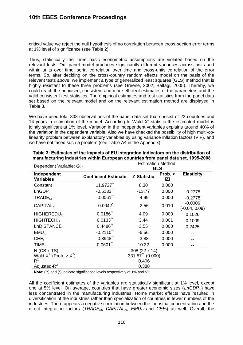
10th EBES Conference Proceedings
116
critical value we reject the null hypothesis of no correlation between cross-section error terms at 1% level of significance (see Table 2). Thus, statistically the three basic econometric assumptions are violated based on the relevant tests. Our panel model produces significantly different variances across units and within units over time, serial correlation over time and cross-units correlation of the error terms. So, after deciding on the cross-country random effects model on the basis of the relevant tests above, we implement a type of generalized least squares (GLS) method that is highly resistant to these three problems (see Greene, 2002; Baltagi, 2005). Thereby, we could reach the unbiased, consistent and more efficient estimates of the parameters and the valid consistent test statistics. The empirical estimates and test statistics from the panel data set based on the relevant model and on the relevant estimation method are displayed in Table 3. We have used total 308 observations of the panel data set that consist of 22 countries and 14 years in estimation of the model. According to Wald X2 statistic the estimated model is
jointly significant at 1% level. Variation in the independent variables explains around 40% of the variation in the dependent variable. Also we have checked the possibility of high multi-co-linearity problem between explanatory variables by using variance inflation factors (VIF), and we have not faced such a problem (see Table A4 in the Appendix).
Table 3: Estimates of the impacts of EU integration indicators on the distribution of manufacturing industries within European countries from panel data set, 1995-2008
Dependent Variable: Gr,t Estimation Method:
GLS
Independent Variables Coefficient Estimate Z-Statistic Prob. >
ǀZǀ Elasticity
Constant 11.9727** 8.30 0.000 --
LnGDPr,t -0.5133** -13.77 0.000 -0.2775
TRADEr,t -0.0061** -4.99 0.000 -0.2778
CAPITALr,t -0.0042* -2.56 0.010 -0.0006
(-0.04, 0.09)
HIGHEREDUr,t 0.0186** 4.09 0.000 0.1026
HIGHTECHr,t 0.0133** 3.44 0.001 0.1009
LnDISTANCEr 0.4486** 3.55 0.000 0.2425
EMUr,t -0.2110** -6.56 0.000 --
CEEr -0.3948** -3.88 0.000 --
TIMEt 0.0601** 10.32 0.000 --
N (CS x TS) Wald X2 (Prob. > X2)
R2
Adjusted-R2
308 (22 x 14) 331.57** (0.000)
0.406 0.388
Note: (**) and (*) indicate significance levels respectively at 1% and 5%. All the coefficient estimates of the variables are statistically significant at 1% level, except one at 5% level. On average, countries that have greater economic sizes (LnGDPr,t) have
less concentrated in the manufacturing industries. Home market effects have resulted in diversification of the industries rather than specialization of countries in fewer numbers of the industries. There appears a negative correlation between the industrial concentration and the direct integration factors (TRADEr,t, CAPITALr,t, EMUr,t and CEEr) as well. Overall, the
10th EBES Conference Proceedings
117
European integration process has lessened the concentration rather than led to the specialization of countries in fewer industries of the manufacturing. Higher rates of trade volumes and net private capital inflows have caused the countries to diversify across the industries. EMU members and CEE countries have concentrated respectively about 0.21 and 0.39 points of less than the rest of the countries in the sample as given the average value of the concentration index (Gr,t) is 1.85.
On the other hand, countries that have the greater rates of higher education graduates in population (HIGHEREDUr,t) and of high-tech product exports in total exports (HIGHTECHr,t)
have concentrated in fewer numbers of the industries. So, human capital and high technology capacity have caused the countries to specialize in certain industries. Also, countries that are at the more distant geography from the European market core (LnDISTANCEr) have specialized relatively more in certain industries. Moreover, overall the
factors beyond those covered in the model have led the countries to concentrate in certain manufacturing industries over time (TIMEt).
Furthermore, because of using differently defined variables in the model in order to compare their impact sizes we have calculated the elasticity coefficients of the relevant variables based on the coefficient estimates and the values of the variables. The elasticity coefficients are displayed at the last column of Table 3. On average, external trade volume and size of national economy have the highest impacts on the dispersion of manufacturing industries in European countries, whereas net foreign private capital inflows have relatively much smaller impact on that. For instance, if an ordinary country has higher GDP or higher rate of external trade volume by a 10%, it would have a lower concentration by about 2.8%, which would have a concentration coefficient of 1.80 points instead of the average of 1.85 points by about 0.05 points of less. Nevertheless, if a country has higher rate of private foreign capital inflows than the ordinary one by a 10%, then it would have a lower concentration than that by only about 0.006%; if the country has the highest rate of net inflows, then it would have a lower concentration than the mean country by around 0.4%; or if the country has the highest rate of net outflows, then it would have a higher concentration by around 0.9% than the representative country. On the other hand, distance to the European core market has the highest impact on the concentration and specialization of European countries in fewer numbers of manufacturing industries. Human capital and technology indicators follow it by the impacts less than its half size of that. For example, if a country has a longer distance than the representative one to the European core by a 10% (i.e., 1100 km. instead of 1000 km.), then it would have a greater concentration by about 2.4%. However, if a country has a greater ratio of higher education graduates to the population or a greater ratio of exports of high-tech products to the total exports relative to the ordinary country by 10%, then it would have a higher concentration and specialization of the industries by around 1% relative to the representative country. 3.2. Results from country by country estimates on time series data European countries are heterogeneous in many specific characteristics, so it is quite plausible they have different trajectories of concentration or diversification in manufacturing industries. Also, the disparate specialization or dispersion paths of the countries in the industries could have been affected diversely by different factors. Therefore, we examine the impacts of the integration indicators on the industrial concentration (specialization) of countries one by one over their time series data, in addition to the overall investigation over the panel data. We first employ the six variables of time-series variant and cross-countries
10th EBES Conference Proceedings
118
invariant from the ones in the earlier panel model (Eq. 2) for each country (Eq. 3) and then select the most efficient model of estimation based on Akaike Information Criterion (AIC). Given the 14 observations of annual time series data and hence the concern that the confidence to the empirical results declines sharply as long as more parameters are imposed on the model with lower degrees of freedom, it seems much better to estimate the model with the least relevant parameters. This approach also helps solve high multi-co-linearity problem, but not totally. Some estimates still contain high collinear variables when the variables of LnGDPt and TIMEt are included in the models of some countries. Half of the country
estimates carry the problem of possible autocorrelation based on the Durbin-Watson (D-W) statistic. In order to minimize this concern we also use Newey-West heteroskedasticity and autocorrelation (HAC) consistent standard errors. So, we should pay extra caution in interpretation of the results. Therefore, we only consider the signs of the significant estimates in our analysis here. Results from the country by country estimates from their time series data sets and their test statistics are given in Table 4. All the estimated models are statistically significant at 1% level except two of them at 5% level by the join F statistic test. Fits of the estimated models into the data distribute roughly between 0.40 and 0.93 by their adjusted R2 values. Growing economic sizes (LnGDPt) of the
10 European countries have significantly affected their further diversification across various manufacturing industries while which have caused the 6 countries to concentrate and specialize more in certain manufacturing industries during the period 1995-2008. However, the developments in economic sizes of the rest 6 countries have not had a significant impact on their industrial distribution. Growing home markets have affected the countries that have the greatest economic sizes differently. Developments in their economic sizes have declined the industrial concentration in Italy (IT) and Great Britain (GB) while they have increased the industrial specialization in Germany (DE) and Spain (ES), but have not had a significant impact on the industrial distribution in France (FR). Only this factor has had a significant impact on the further industrial diversification of Italy and on the further industrial specialization of Ireland (IE). It has caused the industrial dispersion in more of relatively small economies than otherwise. Developments in the foreign trade intensities (TRADEt) have moderated the industrial
concentration in 7 countries (beyond DE and GB, which are relatively small economies) while they have increased it in 3 countries (including FR), but not had a significant impact on the concentration in the rest 12 countries. On the other hand, net foreign private capital movements (CAPITALt ) have surged the industrial concentration in 5 countries (FR and DE, and the 3 relatively small economies) as they have diminished it in 4 countries (including FR), but not had a significant impact on that in the rest 13 countries. So, this factor has not been significantly effective in the industrial concentration of most of the countries. Developments in the higher education graduates (HIGHEREDUt) have increased the
industrial concentration in 6 countries (including GB) and decreased it in 3 countries (including ES), but not significantly affected the industrial distribution in the rest 13 countries. So, this human capital indicator has not been significantly effective in the industrial concentration of most of the countries as well. Developments in the high-tech exports intensities (HIGHTECHt) have escalated the industrial specialization in 7 countries (containing DE and GB) and reduced it in 5 countries (containing FR), but not affected the industrial distribution significantly in the rest 10 countries. Thus, both human capital and technology indicators have appeared to increase (if they could be effective) the industrial concentration and specialization mostly in the relatively small size of economies. Consequently, developments in the factors beyond those contained in the model and
10th EBES Conference Proceedings
119
mentioned above (TIMEt) have raised the industrial specialization in 7 countries and dropped
it in 3 countries, but not affected the industrial distribution in 12 countries during the period. We have observed that all together at least one or more of the integration indicators and/other factors have completely surged the industrial concentration (specialization) only in 3 countries and the industrial diversification only in 2 countries of Europe. In Denmark higher education graduates and exports of high-tech products; in Finland external trade, foreign capital inflows and exports of high-tech products; and in Ireland only the economic size have led only to the further industrial concentration. However, in Italy only the economic size; and in Sweden the economic size and foreign capital inflows have led only to the further industrial diversification. Furthermore, we check whether the integration process has influenced the industrial distribution in the groups of the largest 5 economies and the CEE countries differently. In Germany, the developments in its economic size, net foreign private capital inflows and high-tech exports have increased the concentration and specialization in certain industries as only the development of its external trade has had a significant impact on the industrial diversification during the period. In France, while the external trade and net foreign private capital inflows have surged the further industrial concentration, only the high-tech exports has lessened the industrial specialization. In Great Britain, developments in the economic size and external trade have contributed to the industrial dispersion while higher education graduates and high-tech exports have surged the industrial specialization. In Italy, simply its economic size has had a significant impact on the further industrial diversification. In Spain, while the economic size and the indicators beyond the model have contributed to the industrial concentration, the intensity of higher education graduates has lessened the industrial specialization.
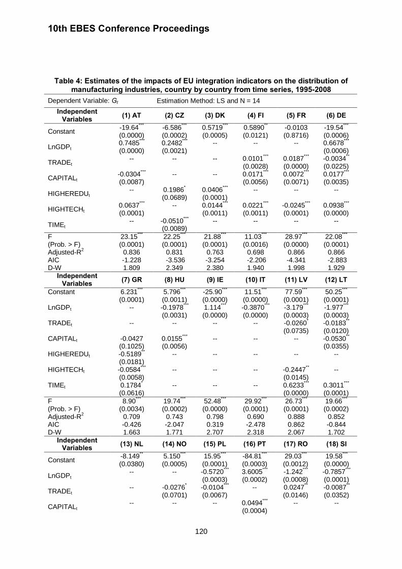
10th EBES Conference Proceedings
120
Table 4: Estimates of the impacts of EU integration indicators on the distribution of
manufacturing industries, country by country from time series, 1995-2008 Dependent Variable: Gt Estimation Method: LS and N = 14
Independent Variables
(1) AT (2) CZ (3) DK (4) FI (5) FR (6) DE
Constant -19.64
***
(0.0000) -6.586
***
(0.0002) 0.5719
***
(0.0005) 0.5890
**
(0.0121)
-0.0103 (0.8716)
-19.54***
(0.0006)
LnGDPt 0.7485
***
(0.0000) 0.2482
***
(0.0021) --
--
--
0.6678***
(0.0006)
TRADEt --
--
--
0.0101***
(0.0028)
0.0187***
(0.0000) -0.0034
**
(0.0225)
CAPITALt -0.0304
***
(0.0087) --
--
0.0171***
(0.0056)
0.0072***
(0.0071) 0.0177
***
(0.0035)
HIGHEREDUt --
0.1986*
(0.0689) 0.0406
***
(0.0001) --
--
--
HIGHTECHt 0.0637
***
(0.0001) --
0.0144***
(0.0011) 0.0221
***
(0.0011)
-0.0245***
(0.0001)
0.0938***
(0.0000)
TIMEt --
-0.0510***
(0.0089)
--
--
--
--
F
(Prob. > F)
Adjusted-R2
AIC D-W
23.15***
(0.0001)
0.836 -1.228 1.809
22.25***
(0.0001)
0.831 -3.536 2.349
21.88***
(0.0001) 0.763 -3.254 2.380
11.03***
(0.0016) 0.698
-2.206 1.940
28.97***
(0.0000) 0.866 -4.341 1.998
22.08***
(0.0001) 0.866
-2.883 1.929
Independent Variables
(7) GR (8) HU (9) IE (10) IT (11) LV (12) LT
Constant 6.231***
(0.0001) 5.796
***
(0.0011) -25.90
***
(0.0000) 11.51
***
(0.0000) 77.59
***
(0.0001) 50.25
***
(0.0001) LnGDPt -- -0.1978
***
(0.0031) 1.114
***
(0.0000) -0.3870
***
(0.0000) -3.179
***
(0.0003) -1.977
***
(0.0003)
TRADEt -- -- -- -- -0.0260*
(0.0735) -0.0183
**
(0.0120) CAPITALt -0.0427
(0.1025) 0.0155
***
(0.0056) -- -- -- -0.0530
**
(0.0355) HIGHEREDUt -0.5189
**
(0.0181) -- -- -- -- --
HIGHTECHt -0.0584***
(0.0058)
-- -- -- -0.2447**
(0.0145)
--
TIMEt 0.1784*
(0.0616) -- -- -- 0.6233
***
(0.0000) 0.3011
***
(0.0001)
F (Prob. > F)
Adjusted-R2
AIC D-W
8.90***
(0.0034) 0.709 -0.426 1.663
19.74***
(0.0002) 0.743 -2.047 1.771
52.48***
(0.0000) 0.798 0.319 2.707
29.92***
(0.0001) 0.690 -2.478 2.318
26.73***
(0.0001) 0.888 0.862 2.067
19.66***
(0.0002) 0.852 -0.844 1.702
Independent Variables
(13) NL (14) NO (15) PL (16) PT (17) RO (18) SI
Constant -8.149
**
(0.0380) 5.150
***
(0.0005) 15.95
***
(0.0001)
-84.81***
(0.0003)
29.03***
(0.0012)
19.58***
(0.0000)
LnGDPt -- -- -0.5720
***
(0.0003)
3.6005***
(0.0002)
-1.242***
(0.0008) -0.7857
***
(0.0001)
TRADEt --
-0.0276*
(0.0701) -0.0104
***
(0.0067)
--
0.0247**
(0.0146)
-0.0087**
(0.0352)
CAPITALt -- -- -- 0.0494
***
(0.0004)
-- --
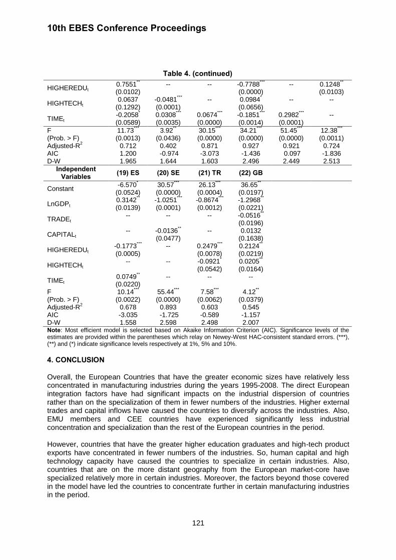
10th EBES Conference Proceedings
121
Table 4. (continued)
HIGHEREDUt 0.7551
**
(0.0102) --
-- -0.7788
***
(0.0000)
--
0.1248**
(0.0103)
HIGHTECHt 0.0637
(0.1292) -0.0481
***
(0.0001)
-- 0.0984*
(0.0656)
-- --
TIMEt -0.2058
*
(0.0589) 0.0308
***
(0.0035) 0.0674
***
(0.0000)
-0.1851***
(0.0014)
0.2982***
(0.0001)
--
F
(Prob. > F)
Adjusted-R2
AIC D-W
11.73***
(0.0013) 0.712 1.200 1.965
3.92**
(0.0436) 0.402
-0.974 1.644
30.15***
(0.0000) 0.871 -3.073 1.603
34.21***
(0.0000) 0.927 -1.436 2.496
51.45***
(0.0000) 0.921 0.097 2.449
12.38***
(0.0011) 0.724 -1.836 2.513
Independent Variables
(19) ES (20) SE (21) TR (22) GB
Constant -6.570
*
(0.0524)
30.57***
(0.0000)
26.13***
(0.0004)
36.65**
(0.0197)
LnGDPt 0.3142
**
(0.0139)
-1.0251***
(0.0001)
-0.8674***
(0.0012)
-1.2968**
(0.0221)
TRADEt -- -- -- -0.0516
**
(0.0196)
CAPITALt --
-0.0136**
(0.0477)
-- 0.0132 (0.1638)
HIGHEREDUt -0.1773
***
(0.0005)
--
0.2479***
(0.0078) 0.2124
**
(0.0219)
HIGHTECHt -- -- -0.0921
*
(0.0542) 0.0205
**
(0.0164)
TIMEt 0.0749
**
(0.0220)
-- -- --
F
(Prob. > F)
Adjusted-R2
AIC D-W
10.14***
(0.0022) 0.678 -3.035 1.558
55.44***
(0.0000) 0.893
-1.725 2.598
7.58***
(0.0062) 0.603 -0.589 2.498
4.12**
(0.0379) 0.545 -1.157 2.007
Note: Most efficient model is selected based on Akaike Information Criterion (AIC). Significance levels of the estimates are provided within the parentheses which relay on Newey-West HAC-consistent standard errors. (***), (**) and (*) indicate significance levels respectively at 1%, 5% and 10%.
4. CONCLUSION Overall, the European Countries that have the greater economic sizes have relatively less concentrated in manufacturing industries during the years 1995-2008. The direct European integration factors have had significant impacts on the industrial dispersion of countries rather than on the specialization of them in fewer numbers of the industries. Higher external trades and capital inflows have caused the countries to diversify across the industries. Also, EMU members and CEE countries have experienced significantly less industrial concentration and specialization than the rest of the European countries in the period. However, countries that have the greater higher education graduates and high-tech product exports have concentrated in fewer numbers of the industries. So, human capital and high technology capacity have caused the countries to specialize in certain industries. Also, countries that are on the more distant geography from the European market-core have specialized relatively more in certain industries. Moreover, the factors beyond those covered in the model have led the countries to concentrate further in certain manufacturing industries in the period.
10th EBES Conference Proceedings
122
On average, external trade and size of national economy have the highest impacts on the dispersion of manufacturing industries in the countries. However, distance to the European market-core has the highest impact on the concentration and specialization of European countries in fewer numbers of the industries. Human capital and technology indicators follow it by the impacts less than its half size of that. On the other hand, due to solely some of the measured integration indicators and measured other factors contained in the model, we have observed a definite industrial concentration only in 3 countries (Denmark, Finland and Ireland) and a definite industrial diversification only in 2 countries (Italy and Sweden) of Europe. In general, the integration indicators and other factors have affected the industrial distributions of European countries differently during the period. Growing economic sizes of the countries and external trades have significantly affected their further diversification across various industries in more instances, particularly in more of the relatively small economies during the period. However, net foreign capital inflows have surged the industrial concentration only in 5 countries. Both human capital and technology indicators have appeared to increase (if they could be effective) the industrial concentration and specialization mostly in the relatively small size of economies. Consequently, developments in the factors beyond those contained in the model have raised the industrial specialization in 7 countries and dropped it in 3 countries, but not affected the industrial distribution in the rest during the period. So briefly, some of the integration indicators and other factors have caused the industrial dispersion in more of the relatively small economies than otherwise. Furthermore, we could not observe a certain pattern for the 5 greatest sizes of economies. Developments in the economic sizes and external trade have increased the industrial dispersion in major part of the CEE countries, whereas the factors beyond the model have had significant impact on the further industrial concentration in most CEE countries. In Turkey, developments in the economic size and exports of high-tech products have encouraged the diversification of manufacturing industries, whereas merely the increasing higher education graduates have strengthened the industrial concentration during the period 1995-2008. REFERENCES Allen, R. C., 2012. Technology and the great divergence: Global economic development since 1820. Explorations in Economic History, 49(1), pp.1-16.
Amiti, M.,1999. Specialization patterns in Europe. Weltwirtschaftliches Archiv,135, pp.1-21.
Asteriou, D. and Hall, S.G., 2007. Applied econometrics. New York: Palgrave Macmilan.
Baltagi, B., 2005. Econometric analysis of panel data. Third Edition. UK: John Wiley & Sons
Ltd. Barrell, R. and Pain, N., 1999. Domestic institutions, agglomerations and foreign direct investment in Europe, European Economic Review, 43(4-6), pp.925-934.
Barro, R.J. and Sala-i-Martin, X., 1992. Convergence. Journal of Political Economy, 100(2),
pp.223-251. Canova, F. and Marcet, A., 1995. The poor stay poor: Non-convergence across countries and regions. Discussion Paper, 1265.
10th EBES Conference Proceedings
123
Combes, P.P.,Overman H.G., 2003. The Spatial distribution of economic activities in the European Union. In: J.V. Henderson and J. F. Thisse, eds. Handbook of regional and urban economics, edition 1, volume 4, Netherlands: North Holland. pp.2845-2909. Dervis, K., 2012. World economy: Convergence, interdependence, and divergence. Finance & Development ,September, pp. 10-14. Desdoigts, A., 1999. Patterns of economic development and the formation of clubs. Journal of Economic Growth ,4, pp. 305-330. Duranton, G., 2008. Spatial economics. In: Steven N. Durlauf and Lawrence E. Blume, eds. The New Palgrave Dictionary of Economics. Second Ed., Palgrave Macmillan: England.
Ellison, G. and Glaeser E. L., 1997. Geographic concentration in US manufacturing industries: A dartboard approach. Journal of Political Economy, 105(5), pp. 889-927.
EU Commission, 2012. [online] Available at: Regional policy presentations. <http://ec.europa.eu/regional_policy /information/presentations/index_en.cfm> [Accessed 05. 12. 2012]. Europa, 2012. [online] Available at: <http://europa.eu/about-eu/basic-
information/index_en.htm> [Accessed 09.12. 2012)
Fujita, M., 2010. The evolution of spatial economics: From Thünen to the new economic geography. Japanese Economic Review, 61 (1), pp.1-32.
Fujita, M., and Thisse, J. F., 2009. New economic geography: An appraisal on the occasion of Paul Krugman’s 2008 Nobel prize in economic sciences. Regional Science and Urban Economics, 39(2), pp.109-119.
Greene, W.H., 2002. Econometric analysis. Fifth Edition. New-York: Prentice Hall.
Hall, R. E. and Jones, C. I., 1999. Why do some countries produce so much more output than others? Quarterly Journal of Economics, 114(1), pp.83-116. Helble, M., Shepherd, B., Wilson, JS., 2007. Transparency, trade costs and regional integration in Asia Pasific. Policy Research Working Paper, 4401. Howitt, P., 2000. Endogenous growth and cross-country income differences. American Economic Review, 90(4), pp.829-846. Islam, N., 1995. Growth empirics: A panel data approach. Quarterly Journal of Economics,
110(4), pp.1127-1170. Islam, N., 2003. What have we learnt from the convergence debate? Journal of Economic Surveys, 17(3), pp.309-362.
Krugman, P., 1991. Increasing returns and economic geography. Journal of Political Economy, 99(31), pp.483-499.
10th EBES Conference Proceedings
124
Levin, A., Linn, C., and Chu, C.J., 2002. Unit root test in panel data: Asymptotic and finite-sample properties, Journal of Econometrics, 108(2002), pp.1-24.
Lucas, R.E., 1988. On the mechanics of economic development. Journal of Monetary Economics, 22(1988), pp.3-42.
Lucas, R.E., 1990. Why doesn`t capital flow from rich to poor countries? American Economic Review, 80(2), pp.92-96.
Mankiw, N.G., Romer, D., and Weil, D., 1992. A Contribution to the empirics of economic growth. Quarterly Journal of Economics, 107(May), pp.407-437.
North, D. C., 1990. Institutions, institutional change, and economic performance. Cambridge
MA and New York: Cambridge University Press. Ottoviano, G., 1999. Integration, geography and the burden of history. Regional Science and Urban Economics, 29(2), pp.245-256. Ottoviano, G. and Thisse, J. F., 2002. Integration, agglomeration and political economics of factor mobility. Journal of Public Economics, 83(2002), pp.429-456 Pflüger, M. and Südekom, J., 2007. Integration, agglomeration and welfare. Journal of Urban Economics, 63(2), pp.544-566.
Pritchett, L., 1997. Divergence, big time. Journal of Economic Perspectives, 11(3), pp.3-17.
Quah, D., 1990. International patterns of economic growth: I. persistence in cross-country disparities. Cambridge: MIT Press.
Quah, D., 1996. Convergence empirics across economies with (some) capital mobility. Journal of Economic Growth, 1(1), pp.95-124. Reynolds, C.R., 1997. Open regionalizm: Learnings from Latin America for East Asia. Kellogg Institute Working Paper, 241. Rodrick, D., 2011. The future of economic convergence. NBER Working Paper, 17400.
Romer, P., 1986. Increasing returns and long run growth. Journal of Political Economy, 94(5), pp.1002-1036. Romer, P., 1990. Endogenous technological change. Journal of Political Economy, 98(5), pp.71-102. Royo, S., 2010. Portugal and Spain in the EU: Paths of economic divergence (2000-2007). Analise Social, 45(195), pp.209-254.
Sala-i-Martin, X., 1996. The classical approach to convergence analysis. The Economic Journal, 106(437), pp.1019-1036.
Solow, R.M., 1956. A contribution to the theory of economic growth. Quarterly Journal of Economics, 70(1), pp.65-94.

10th EBES Conference Proceedings
125
Westerlund, J., 2007. Testing for error correction in panel data. Oxford Bulletin of Economics and Statistics, 69(6), pp.709-748.
Wooldridge, J.M., 2002. Introductory econometrics: A modern approach, South-Western, 2nd Revised Edition. USA: Division of Thomson Learning.
Tatoglu, Y.F., 2012. Panel veri ekonometrisi [Panel data econometrics]. İstanbul: Beta Yayınevi. APPENDIX A: Definitions of Variables and Sources of Data
Table A1. European Countries Employed in the Analysis and their Situations in the EU
Integration
No Cod Country EU member
(years) EMU member
(years) CEE
country 1 AT Austria (-1995-2008+) (1999-2008+) --
2 CZ Czech Republic (2004-2008+) -- Yes
3 DK Denmark (-1995-2008+) -- --
4 FI Finland (-1995-2008+) (1999-2008+) --
5 FR France (-1995-2008+) (1999-2008+) --
6 DE Germany (-1995-2008+) (1999-2008+) --
7 GR Greece (-1995-2008+) (2001-2008+) --
8 HU Hungary (2004-2008+) -- Yes
9 IE Ireland (-1995-2008+) (1999-2008+) --
10 IT Italy (-1995-2008+) (1999-2008+) --
11 LV Latvia (2004-2008+) -- Yes
12 LT Lithuania (2004-2008+) -- Yes
13 NL Netherlands (-1995-2008+) (1999-2008+) --
14 NO Norway -- -- (Yes)
15 PL Poland (2004-2008+) -- Yes
16 PT Portugal (-1995-2008+) (1999-2008+) --
17 RO Romania (2007-2008+) -- Yes
18 SI Slovenia (2004-2008+) (2007-2008+) Yes
19 ES Spain (-1995-2008+) (1999-2008+) --
20 SE Sweden (-1995-2008+) -- --
21 TR Turkey -- -- (Yes)
22 GB United Kingdom (-1995-2008+) -- --
Note: Even though Norway and Turkey are not EU and CEE countries, they are represented as in the CEE group in the CEE dummy.

10th EBES Conference Proceedings
126
Table A2. Manufacturing Industries Employed in the Analysis (ISIC Rev-3)
No Cod Sectors 1 15 Manufacture of Food Products and Beverages
2 16 Manufacture of Tobacco Products
3 17 Manufacture of Textiles
4 18 Manufacture of Wearing Apparel; Dressing and Dyeing of Fur
5 19 Tanning and Dressing of Leather; Manufacture of Luggage, Handbags, Saddlers, Harness and Footwear
6 20 Manufacture of Wood and of Products of Wood and Cork, except Furniture; Manufacture of articles o
7 21 Manufacture of Paper and Paper Products
8 22 Publishing, Printing and Reproduction of Recorded Media
9 23 Manufacture of Coke, Refined Petroleum Products and Nuclear Fuel
10 24 Manufacture of Chemicals and Chemical Products
11 25 Manufacture of Rubber and Plastics Products
12 26 Manufacture of Other Non-Metallic Mineral Products
13 27 Manufacture of Basic Metals
14 28 Manufacture of Fabricated Metal Products, except Machinery and Equipment
15 29 Manufacture of Machinery and Equipment NEC
16 30 Manufacture of Office, Accounting and Computing Machinery
17 31 Manufacture of Electrical Machinery and Apparatus NEC
18 32 Manufacture of Radio, Television and Communication Equipment and Apparatus
19 33 Manufacture of Medical, Precision and Optical Instruments, Watches and Clocks
20 34 Manufacture of Motor Vehicles, Trailers and Semi-Trailers
21 35 Manufacture of other Transport Equipment
22 36 Manufacture of Furniture; Manufacturing NEC
23 37 Recycling
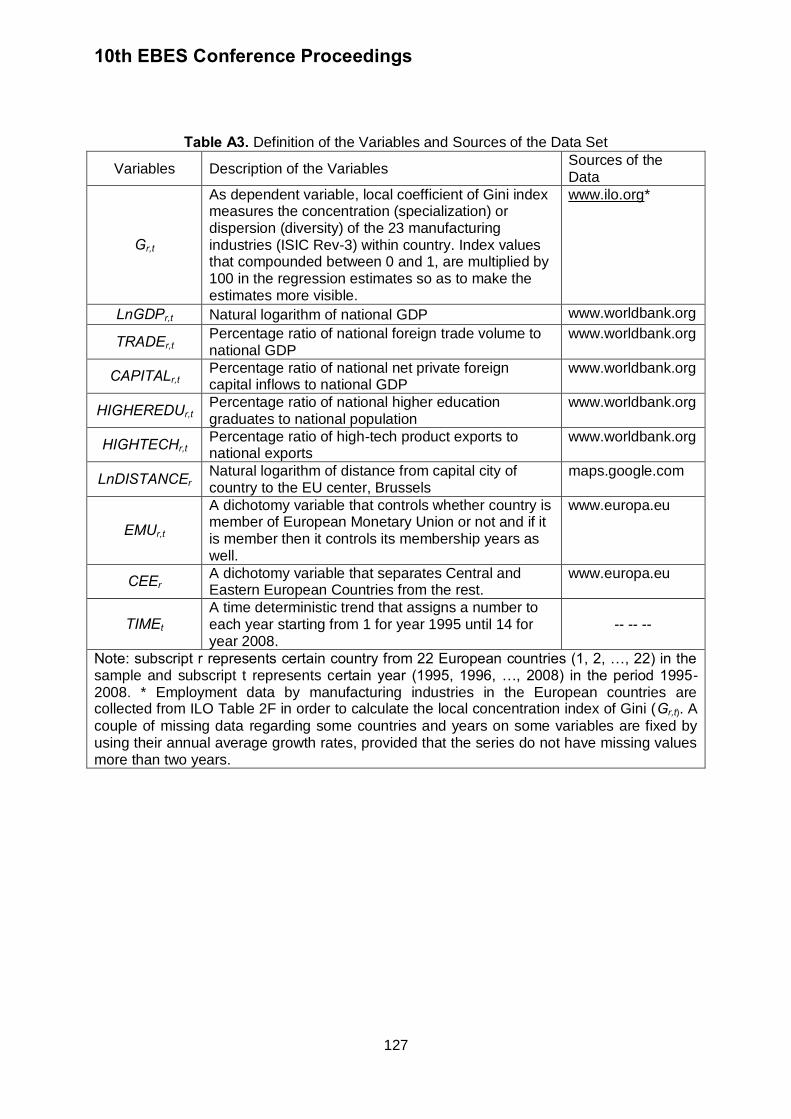
10th EBES Conference Proceedings
127
Table A3. Definition of the Variables and Sources of the Data Set
Variables Description of the Variables Sources of the Data
Gr,t
As dependent variable, local coefficient of Gini index measures the concentration (specialization) or dispersion (diversity) of the 23 manufacturing industries (ISIC Rev-3) within country. Index values that compounded between 0 and 1, are multiplied by 100 in the regression estimates so as to make the estimates more visible.
www.ilo.org*
LnGDPr,t Natural logarithm of national GDP www.worldbank.org
TRADEr,t Percentage ratio of national foreign trade volume to national GDP
www.worldbank.org
CAPITALr,t Percentage ratio of national net private foreign capital inflows to national GDP
www.worldbank.org
HIGHEREDUr,t Percentage ratio of national higher education graduates to national population
www.worldbank.org
HIGHTECHr,t Percentage ratio of high-tech product exports to national exports
www.worldbank.org
LnDISTANCEr Natural logarithm of distance from capital city of country to the EU center, Brussels
maps.google.com
EMUr,t
A dichotomy variable that controls whether country is member of European Monetary Union or not and if it is member then it controls its membership years as well.
www.europa.eu
CEEr A dichotomy variable that separates Central and Eastern European Countries from the rest.
www.europa.eu
TIMEt A time deterministic trend that assigns a number to each year starting from 1 for year 1995 until 14 for year 2008.
-- -- --
Note: subscript r represents certain country from 22 European countries (1, 2, …, 22) in the sample and subscript t represents certain year (1995, 1996, …, 2008) in the period 1995-2008. * Employment data by manufacturing industries in the European countries are collected from ILO Table 2F in order to calculate the local concentration index of Gini (Gr,t). A
couple of missing data regarding some countries and years on some variables are fixed by using their annual average growth rates, provided that the series do not have missing values more than two years.
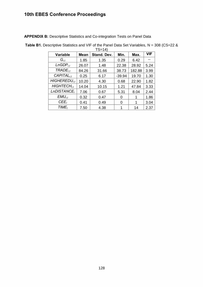
10th EBES Conference Proceedings
128
APPENDIX B: Descriptive Statistics and Co-integration Tests on Panel Data
Table B1. Descriptive Statistics and VIF of the Panel Data Set Variables, N = 308 (CS=22 &
TS=14)
Variable Mean Stand. Dev. Min. Max. VIF Gr,t 1.85 1.35 0.29 6.42 --
LnGDPr,t 26.07 1.48 22.38 28.92 5.24
TRADEr,t 84.26 31.66 38.73 182.88 3.99
CAPITALr,t 0.25 6.17 -39.94 19.70 1.30
HIGHEREDUr,t 10.20 4.30 0.68 22.90 1.82
HIGHTECHr,t 14.04 10.15 1.21 47.84 3.33
LnDISTANCEr 7.06 0.67 5.31 8.04 2.44
EMUr,t 0.32 0.47 0 1 1.86
CEEr 0.41 0.49 0 1 3.04
TIMEt 7.50 4.38 1 14 2.37
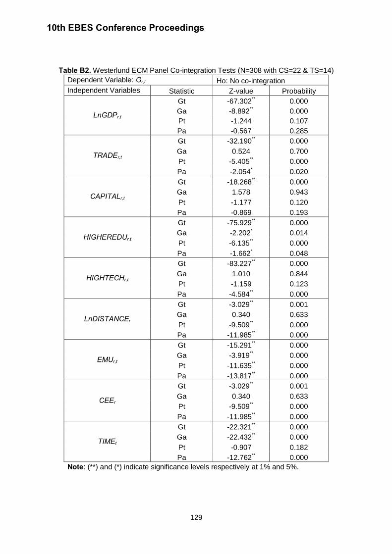
10th EBES Conference Proceedings
129
Table B2. Westerlund ECM Panel Co-integration Tests (N=308 with CS=22 & TS=14)
Dependent Variable: Gr,t
Ho: No co-integration
Independent Variables Statistic Z-value Probability
LnGDPr,t
Gt -67.302** 0.000
Ga -8.892** 0.000
Pt -1.244 0.107
Pa -0.567 0.285
TRADEr,t
Gt -32.190** 0.000
Ga 0.524 0.700
Pt -5.405** 0.000
Pa -2.054* 0.020
CAPITALr,t
Gt -18.268** 0.000
Ga 1.578 0.943
Pt -1.177 0.120
Pa -0.869 0.193
HIGHEREDUr,t
Gt -75.929** 0.000
Ga -2.202* 0.014
Pt -6.135** 0.000
Pa -1.662* 0.048
HIGHTECHr,t
Gt -83.227** 0.000
Ga 1.010 0.844
Pt -1.159 0.123
Pa -4.584** 0.000
LnDISTANCEr
Gt -3.029** 0.001
Ga 0.340 0.633
Pt -9.509** 0.000
Pa -11.985** 0.000
EMUr,t
Gt -15.291** 0.000
Ga -3.919** 0.000
Pt -11.635** 0.000
Pa -13.817** 0.000
CEEr
Gt -3.029** 0.001
Ga 0.340 0.633
Pt -9.509** 0.000
Pa -11.985** 0.000
TIMEt
Gt -22.321** 0.000
Ga -22.432** 0.000
Pt -0.907 0.182
Pa -12.762** 0.000
Note: (**) and (*) indicate significance levels respectively at 1% and 5%.

10th EBES Conference Proceedings 23 - 25 May, 2013. NIPPON HOTEL, ISTANBUL, TURKEY ISBN: 978-605-64002-1-6. WEBSITE: www.ebesweb.org
130
CVaR-E(r) EQUILIBRIUM ASSET PRICING
MIHALY ORMOS Department of Finance
Budapest University of Technology and Economics Hungary
DUSAN TIMOTITY Department of Finance
Budapest University of Technology and Economics Hungary
[email protected] Abstract: We introduce a novel equilibrium asset-pricing model, which we build on the relationship between Conditional Value-at-Risk (CVaR) and the expected return. This approach of risk measure allows us to get rid of the normality condition of returns. Combining the CVaR risk measure method with our regression model, nonrealistic assumptions – such as rational and risk–averse investors, unlimited leverage opportunity and price-taker investors – of the most commonly used models can be almost entirely omitted. In our model we define the optimal choice for every single investor. Aggregating the required returns, allows us including different leverage constraints and margins, thus we do not assume unlimited borrowing for risk-free interest rate. Furthermore, based on the anchoring effect in Prospect Theory risk-seeking behavior can be explained and implemented in our model. On the other hand, the aggregation method to calculate expected returns allows price-maker investors having great influence on price movements (in case of a block transaction or in a non-liquid market segment). Keywords: Behavioral Finance, Asset Pricing, Prospect Theory, Anchoring, Conditional Value-at-Risk 1. INTRODUCTION We construct an equilibrium asset pricing model that, contrasting the standard models using Expected Utility Theory (EUT), is based on loss-averse investors described by the Prospect Theory (Kahneman and Tversky, 1979). We approximate loss-aversion by Value-at-Risk (Campbell et al. 2001; Jorion, 2007) and Conditional–Value–at–Risk (Rockafellar and Uryasev, 2000), by which we can define the expected loss weighted by its probability. We apply the assumption that in some cases investors define a reference point on their utility curve, resulting in an anchoring, thus they do not refuse risk, moreover they start to follow risk-seeking behavior to an extent (Ariely et al. 2003), since their expected utility can be maximized in this behavior. Furthermore, our regression is more realistic than standard asset pricing models from another point of view, namely we do not assume the returns to be normally distributed. The results we present in this paper somewhat different from the well known models approximating expected return by standard deviation – such as the Modern Portfolio Theory (Markowitz, 1959), or the Capital Asset Pricing Model (CAPM) (Sharpe, 1964; Lintner, 1965; Mossin, 1966) –, as we change the risk parameter from standard deviation to Conditional–Value–at–Risk (CVaR). Our model omits the assumption of price–taker investors and allows significant price–making activity by block transactions or in non–liquid market segments. We also allow limited borrowings, different leverage constraints and interest rates for every single investor. Therefore, we define a more realistic and precise way to explain individual optimization method, and by approximating the expected return through
10th EBES Conference Proceedings
131
the aggregation of investors' required returns, we create a model that describes expected return without using the most significant unrealistic assumptions of standard asset pricing models. About fifty years ago, importance of asset pricing has reached a point that it required a model. Scholars in the field have built the first regressions in order to have at least one asset-pricing model. Investors often use these approximations nowadays too, however, these standard models had many unrealistic assumptions that could be omitted applying modern technological background. The most commonly used model, the CAPM defines three area of limitation: the first states there is a perfect market consisting of four assumptions (1) investors have constant preferences, (2) are price–takers, (3) are perfectly informed and (4) there is no transaction cost. The second area of limitation describes the investors' behavior stating that (1) they are rationally risk–averse, therefore they hold efficient portfolios defined by Markowitz and (2) due to their rationality and perfect information have homogenous expectations. The last area of limitation states that (1) there exist risk–free assets besides risky portfolios and (2) they can borrow infinite amount of money on this risk–free interest rate. Through our model the assumptions of risk–averse and price–taker investors, normal distribution of returns (thus the required linear regression between risk and expected return (Erdos et al. 2010, 2011)) and unlimited borrowing on risk–free interest rate can be omitted, furthermore using the results of Meng et al. (2011) it can be applied as a multi–period model. In the following chapter we describe the applied sections of the Prospect Theory (Kahneman and Tversky, 1979), in the third section the risk–seeking behavior is introduced, in the fourth section the model is implemented for the above behavior, the fifth section describes the applied CVaR risk measure and its inclusion in our regression, in the sixth section we describe our implementation of limited leverage constraints in the model, in the seventh section we define the expected return calculation using aggregation of individual required returns and at last we summarize the most important results of this research paper. 2. RISK–AVERSION OR LOSS–AVERSION In order to measure risk–taking behavior we define the Arrow–Pratt measure of absolute risk–aversion (ARA) (Pratt, 1964). There are mainly two types of investors, those who follow constant absolute risk–aversion (CARA) and those who have constant relative risk–aversion (CRRA). The first one describes the risk premium necessary to invest in a mathematically fair investment, which does not depend on the reference wealth. The second one states that risk–aversion changes over with the change of wealth but in a constant way meaning that reference wealth multiplied with the ARA is constant over time for each investor. Both measures have advantages and disadvantages over the other, however – in case of small change of wealth –, we can use both of them for any investor. Either examining the utility curve for CARA or for CRRA, the approximation of the utility of investment F (U(F)) using Taylor series is defined by:.
(1) where U(F) means the expected utility of investment F, E(F) is its expected value, a is the Arrow–Pratt measure of absolute risk–aversion and σ2 is the variance that measures the risk of investment F. By accepting the assumptions thatσ2-E(r) efficient combinations can be described by a concave curve with positive slope – or in the case of unlimited borrowings with constant slope – and that investors are risk–averse (hence, their CARA is positive, thus their utility

10th EBES Conference Proceedings
132
curve is convex with monotonic growth), optimal choice can be defined easily for any investor. However, according to the Prospect Theory by Kahneman and Tversky (1979) investors do not behave rationally in every situation, therefore, through the Expected Utility Theory (EUT) some of their actions cannot be explained. The authors underline that investors' decisions–making process is based not solely on economic rationality but subjective elements too, which motivates them to such behavior that would be completely irrational in standard economic theories. According to Shefrin (2002) these behavioral patterns are heuristic–driven biases and frame dependencies. There are numerous heuristics that play important role in decision–making, such as representativeness (meaning that people overestimate the frequency of things surrounding them and make stereotypes), the availability bias (meaning that people rely too strongly on their own experience) or – which is the most important in this paper – the anchoring (meaning that people make reference points and they adjust the new information according to its parameters). These subjective elements cause biases in investors' expected probabilities, therefore they overestimate (and overreact) rare things and underestimate (underreact) frequent things. This phenomenon happens in case of wealth change in both directions, however, in case of gains it causes higher distortion than in case of losses, which can be seen on the Figure 1 (Kahneman and Tversky, 1979).
1
0.9
0.8
0.7
0.6
0.5
0.4
0.3
0.2
0,1
0
10.90.8 0.7 0.6 0.5 0.4 0.3 0.20,1
W +
W -
w(p
) su
bje
ctiv
e w
eigh
t
p probability
Source: http://prospect-theory.behaviouralfinance.net/
Figure 1: Subjective probability in Prospect Theory
Based on the heuristics mentioned above, Daniel Kahneman and Amos Tversky developed a model that – in spite of EUT that defines utility as the function of total wealth (the absolute way) – measures utility through the change of wealth (in a relative way), which seems to be a more precise method to describe investors' behavior. In their theory positive changes of wealth can be described with a function similar to the EUT utility function (which is concave and has monotonic growth), hence, the law of diminishing marginal utility (Gossen, 1854) stays intact. However, in case of negative changes of wealth (losses), although investors keep being risk–averse in normal cases (since their reference point returns to zero and the slope of the curve on loss side is 2,25 times the slope on the gain side, thus their utility decreases 2,25 times more for x loss than it increases for x gain), this utility function

10th EBES Conference Proceedings
133
becomes convex for negative change. Therefore, they define an S–shaped utility curve (Figure 2).
Source: Kahneman and Tversky (1979, p.279)
Figure 2:Utility curve in Prospect Theory 3. RISK–SEEKING DUE TO LOSS–AVERSION Kahneman and Tversky (1979) created a model that allows analyzing single period choices, since according to their theory the investor makes its choice from the zero reference point every time. However, in reality this is not the case every time. Proven by research on the heuristic–driven biases, for different reasons – such as the anchoring effect (adjusting to a reference situation), the inclusion of sunken costs or the sticking effect (investors give up to properly manage their portfolios after a massive loss and do not sell) – investors can be motivated to fix a reference point on their utility curve and keep it at their next decision, which places them to non–zero starting point on their utility curve. This way, one can easily see that there are mathematically fair investments that result in utility growth, therefore, investors maximizing the variance of the chosen fair investment – until an optimal value – can increase their utility gain for fixed expected return. Hence, this is by definition risk–seeking behavior. This situation can be seen on the Figure 3 where we used the exponential utility function for CARA, the ( . The calculation of the function is based on the equation
(1)
where a=5 is an average measure of constant absolute risk–aversion and x = -5% is the negative return as reference point after 5% loss. Based on the results, in this case investors are risk–seeking until they are able to reach 7.72% return on the positive side.

10th EBES Conference Proceedings
134
Figure 3: Fair investment after previous loss
Since if x < 0, than U(x) = - 2.25U(-x) in average and the investor maximize the risk (here the variance) until the utility growth due to positive wealth change y is greater than utility loss due to negative wealth change where he/she becomes risk–neutral, the risk–neutral curve can be defined using the following equation. Here, we simulate a mathematically fair investment consisting of (x + y) gain and(-x - y) loss both with 50% probability. The reference point is (-x). The investor keeps following risk–seeking behavior until the utility growth and loss get to be equal, therefore: (2) Through defining the utility on the negative side by its positive equivalent, due to the 2.25 multiplicator, we get: (3) therefore: (4) we can define an alternative version of this by:
(5)
From this equation it can be seen that due to the law of diminishing marginal utility [2U(x)+U(y)-U(2x+y)]>0, therefore, U(y) and y have to be positive in order to have solution for the equation. The exact shape of the utility function can define these precise solutions. As for the variance of this investment, starting from -x reference point choosing the mathematically fair investment with (x+y) amplitude, we can define:

10th EBES Conference Proceedings
135
=
(6)
Furthermore, if we simulate an alternative version of this investment with positive expected return, we get similar results. By keeping the -x reference point but instead of 0 we analyze an investment with expected return of 0<c1<x, we get the following situation: In order to have the same utility change – in absolute way – for both negative and positive wealth change with c1expected return (thus for (-x+c1) reference point), it can be seen that the variance has to decrease. The slope of this decrease can be defined by analyzing the utility function: To ensure having a solution to the equation between utility gains and losses we can define the following situation: A mathematically fair investment withc1expected return and with the original reference point of -x the reference point gets to be (-x+c1). As mentioned above, the amplitude that was (x + y) before has to decrease by -c2 in order to keep the equality between utility differences caused by gains and by losses, therefore: (7) Converting the negative side to its positive equivalent again we get: (8) Looking at this equation, that can be seen that in case of c1=0 we get the same result as equation (4) (thus c2=0) and if c1=x, then (9) Due to the multiplier 2.25 equation (9) is solvable only if both sides are 0, therefore, y=c2. According to equation (4):
(10) We define the relation between c1 and c2 by using equation (10) as a function. Assuming that the utility curve is a standard exponential function for constant absolute risk–aversion that is 1-e^-ax with x=c, y=d constant variables, while we substitute c1=x and c2=y variables, the previous equation (10) can be written as the following:
(11)
The total derivative of this function by variable x is:
2 + +4.5 − − − − −1+ − − − − (12)
Since we know that according to equation (10) this function has to be zero for all changes of x, its derivative also has to be zero. The derivative by constant variables is zero, therefore, we get for df/dx:

10th EBES Conference Proceedings
136
(13)
And now we can describe the relation between x and y as dy/dx:
(14)
Since we fixed that y≤d and c≤x, therefore, for every a>0 we get positive result for the numerator and negative result for the denominator. Hence, if x increases, y has to decrease according to equation (14). In case of small changes that can be proven also that for constant relative risk–aversion with
function of
we would have got the same results.
Turning back to our original variable system (x,y,c1,c2) we defined that in case of 0<c1<x this risk–seeking behavior exists, thus we know the interval for variance – expected return combinations also. The shape of the transition function is describes by equation (14). This way we define that starting from the variance – expected return combination (0;x) (the minimum of the interval) to the combination of ((x+y)2;0) investors are maximizing the variance until they reach the "optimal" choice, the risk–neutral curve, which can be seen at Figure 4 (although this is only the approximation of the true shape of the curve). In order to analyze these phenomena, we define that this risk–neutral function is monotonically decreasing, therefore, according to equation (14), as the expected return of the investment (c1) increases the variance (c2) has to decrease. Hence, instead of investment A an investor would choose the investment A' with the same expected return and higher variance, which would completely irrational in standard equilibrium models.
Figure 4: Risk–seeking until risk–neutrality
Although this result based on the variance – expected return relation is important and can be implemented in standard equilibrium models, it necessitates a very strong condition that return distributions have to be symmetric, which is clearly not the case in reality, therefore its use in practice is very limited. Our proposed model uses Conditional–Value–at–Risk (CVaR) as risk measure, which allows us to describe the same situation in an alternative way, thus any type of distribution can be applied in our regression.
(x+y)2
2
x
A A’
E(r)
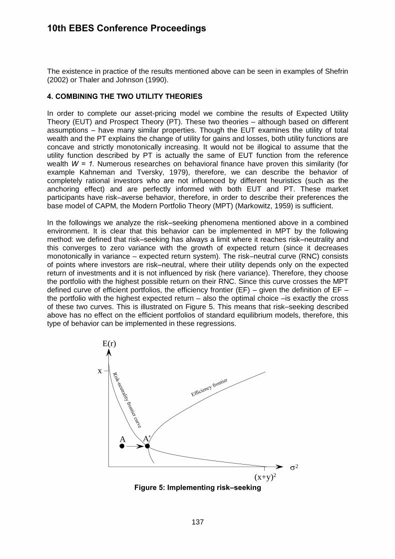
10th EBES Conference Proceedings
137
The existence in practice of the results mentioned above can be seen in examples of Shefrin (2002) or Thaler and Johnson (1990). 4. COMBINING THE TWO UTILITY THEORIES In order to complete our asset-pricing model we combine the results of Expected Utility Theory (EUT) and Prospect Theory (PT). These two theories – although based on different assumptions – have many similar properties. Though the EUT examines the utility of total wealth and the PT explains the change of utility for gains and losses, both utility functions are concave and strictly monotonically increasing. It would not be illogical to assume that the utility function described by PT is actually the same of EUT function from the reference wealth W = 1. Numerous researches on behavioral finance have proven this similarity (for example Kahneman and Tversky, 1979), therefore, we can describe the behavior of completely rational investors who are not influenced by different heuristics (such as the anchoring effect) and are perfectly informed with both EUT and PT. These market participants have risk–averse behavior, therefore, in order to describe their preferences the base model of CAPM, the Modern Portfolio Theory (MPT) (Markowitz, 1959) is sufficient. In the followings we analyze the risk–seeking phenomena mentioned above in a combined environment. It is clear that this behavior can be implemented in MPT by the following method: we defined that risk–seeking has always a limit where it reaches risk–neutrality and this converges to zero variance with the growth of expected return (since it decreases monotonically in variance – expected return system). The risk–neutral curve (RNC) consists of points where investors are risk–neutral, where their utility depends only on the expected return of investments and it is not influenced by risk (here variance). Therefore, they choose the portfolio with the highest possible return on their RNC. Since this curve crosses the MPT defined curve of efficient portfolios, the efficiency frontier (EF) – given the definition of EF – the portfolio with the highest expected return – also the optimal choice –is exactly the cross of these two curves. This is illustrated on Figure 5. This means that risk–seeking described above has no effect on the efficient portfolios of standard equilibrium models, therefore, this type of behavior can be implemented in these regressions.
(x+y)2
2
x
A A’
E(r)
Figure 5: Implementing risk–seeking

10th EBES Conference Proceedings
138
5. THE CVAR RISK MEASURE In this section first we define the meaning of Conditional–Value–at–Risk, its use in financial calculations, then we describe the modified CVaR measure used in our model. Our model includes price–maker investors too, however, for now in order to make our approach easier to understand we assume price–taking investors in a competitive market, which means that they rationally choose investment opportunities from the efficient portfolio frontier (similar to the one in Modern Portfolio Theory (Markowitz, 1959)). 5.1. The definition of Conditional–Value–at–Risk (CVaR) Since the expected return – variance relationship introduced by MPT and the beta in the CAPM numerous attempts were made to offer an alternative risk measure. One of the most important ones was Value–at–Risk (Holton, 2003) that gained popularity amongst quantitative financial professionals in the '80s (mainly due to the crisis in 1987). This measure provided an entirely new method to calculate the true risk of derivatives, options and other non–standard financial assets since it shows the maximal value that investors can lose with a predefined confidential interval (or probability), which is based on the true distribution of these investments. Although it had many advantages over volatility and beta, it missed the important characteristics of sub–additivity and convexity (Rockafellar and Uryasev, 2000). The Conditional–Value–at–Risk was meant to solve these problems, which has made it the most precise risk–measuring technique today (Krokhmal et al. 2002). In order to define CVaR first we introduce the meaning of VaR. The VaR for a fixed α% shows the value that with (1-α)% probability the return of an investment will be above. An alternative explanation is thatVaRα is the α percentile of the distribution function of return. By defining f(x,y) as the function of loss where x is a chosen portfolio and y is a random variable, the probability of f(x,y) not exceeding a ζ value (loss) is ψ,:
(15)
Assuming fixed x portfolio, this equation is the same as the cumulative distribution function of f(x,y) loss function inζ . According to this function the Value–at–Risk (VaRα) is:
α (16)
meaning the first point on the cumulative distribution function of the return of x portfolio with greater cumulative probability than α. CVaRαcan be described the same technique:
(17)
where is (1-α)according the definition of VaR, hence it becomes the denominator. The interpretation of the equations above is that VaRα(x)is the α percentile of f(x,y) loss function, while CVaRα(x) is the probability weighted average (expected value) of losses greater than VaR. Therefore, CVaRα(x)≥VaRα(x) always has to be true (Rockafellar and Uryasev, 2002). Although there are numerous techniques to solve the minimization problem for CVaRα(x) (for example Krokhmal et al. 2002), our main goal was not to describe these methods or the
10th EBES Conference Proceedings
139
calculated efficiency frontier but to combine them with the utility measure in Prospect Theory, hence to describe the optimal choice of investors with precise quantitative analysis. 5.2. CVaR modification and the efficiency frontier Definition of Conditional–Value–at–Risk in our model is somewhat different from the approach in standard methods. Today's techniques used in practice calculate the f(x,y) loss function by defining the value of loss as positive, furthermore, in order to avoid negative results, they for VaRα(x) calculation the max{f(x,y),0} function, therefore neither VaRα(x), nor CVaRα(x) can be negative. In this paper we define CVaRα(x) as a negative measure, thus the loss function produced negative return, while we keep the positive interval of the distribution function for returns lower than the expected return, therefore, we do not cut its value with zero, hence VaRα(x) and CVaRα(x) can be both positive and negative depending on α (positive usually in case of highα). This modification has no effect on calculation methods, however, in our opinion it helps to understand the meaning of CVaRα(x)and to place it in realistic environment. Since we use CVaRα(x) as its true, negative value, our optimization method requires (instead of minimizing) maximizing CVaRα(x) that can exceed 0. We fix the value ofα as 0.5 (50%) because this is optimal to describe the theoretical background. 5.3. Positive time preference and CVaR As mentioned in the previous section, investments can have positive CVaRα(x) if choosing high α for analysis. However, many of the risk measuring methods cannot handle these situations appropriately since they minimize CVaRα(x) with 0, therefore, they disregard the distribution interval for returns below this point. According to this, they miss the difference of two investments having different distribution functions only for positive returns. In order to get rid of this problem measuring the whole negative risk without limits (with 50% α) seems to be a solution, although, on this level fat–tail distributions have less effect on CVaRα(x) calculation. Moreover, with this approach to CVaR positive time preference of investors can be proved. This can be seen through future cash–flows generating positive expected returns even if they are almost entirely risk–free investments. This is due to the positive time preference which means that consumption in the present cause much more utility growth for investors than the same consumption in the future, therefore, they require compensation in the future in exchange for lending money (thus utility) in the present. Hence, investments can be found where CVaRα(x) exceeds 0 because their risk is so low that the average of negative returns is smaller the expected return itself. Put it the other way, if the investment turns out to have smaller return than the expected one, the Conditional–Value–at–Risk gets to be positive, the investor realizes positive expected return in the worst 50% too. This can be interpreted as the risk–free return defined in standard equilibrium asset pricing models, however, in reality none of them are entirely risk–free, therefore CVaRα(x) is always lower than E(r). This can be illustrated by a 45˚ line with s=1 slope on the CVaR-E(r) coordinate system. None of the portfolios can reach the area below this line. The system of {CVaR0.5(x),E(r)} pairs can be seen on Figure 6. The weights and the values of the pairs were calculated by using Monte Carlo simulation with the following data and parameters: we used historical, yearly returns from 1928 to 2011 of 4 different assets: the T-bill with 3 month maturity, the T-bond with 10 year maturity, the S&P 500 index and the Coca-Cola shares (adjusted to splits and dividends). We simulated 10.000 randomly generated portfolios of these and for every portfolio we calculated yearly returns,

10th EBES Conference Proceedings
140
CVaR0.5from their distribution and average (expected) return over the period. The Conditional–Value–at–Risk measure can be seen on the horizontal axis, while the expected return on the vertical axis. It can be clearly seen that the efficiency frontier (the highest expected return for every CVaR value) is very similar to the one in the MPT since it is concave, although its slope is decreasing. Therefore, optimization with utility function (which is convex in MPT) seems to have a unique solution for CVaR equilibrium also. We define this optimum in the next section.
Figure 6: Portfolio plot in CVaR0.5 - E(r) system
In order to show the significance of the use of CVaR risk measure, we created a scatter plot on Figure 7, where CVaR–E(r) pairs can be seen both calculated by using normal distribution and by using the true distribution. Since the expected return is independent of the type of distribution (it is only the probability–weighted average return, E(r)=Σ(wiri,)) it is the same for both cases, however, the value of CVaR is calculated differently in the two cases. It is clear that the CVaR is lower for fixed expected return in the case of true CVaR calculation, which corresponds to the fact the fat–tail distributions have higher risk than the theoretical normal distributions.

10th EBES Conference Proceedings
141
Figure 7: Difference from normal distribution in CVaR0.5 - E(r) system
5.4. Simulating individual choice with CVaR As we mentioned before the level of risk–aversion of an investor can be defined by a unique parameter, the "A" measure of risk–aversion. Since we assume that the Kahneman and Tversky utility function has the same convexity on the right side as the expected utility function in EUT, the behavior of an individual can be described in both risk–averse and risk–seeking cases with the aid of this measure, therefore, our model can define the optimal choice for every investor with the constraints that the goal is utility maximizing and the efficient portfolios have the efficiency frontier. In case of risk–aversion the approximation of expected utility could be used in our model too in the following method: We know that:
(18) For now we use normal distribution as approximation, which allows tighter conditions, thus true distributions can be calculated in the same way. This way we can define CVaR as the function of expected return and variance:1 (19)
According to this, we can substitute the volatility ( ) with the Conditional–Value–at–Risk (CVaR), therefore, the approximating function (18) can be implemented in CVaR-E(r) system:
(20)
Solving the previous equation gives:
1in case of normal distribution CVaR0.5=

10th EBES Conference Proceedings
142
(21)
In order to define E(rx), we examine if the expression containing E(rx) is positive or negative.:
(22)
By solving for E(rx) and introducing the variance again for easier application and for using historical empirical research, normal distribution (where CVaR=E(r)-0.8σ) gives:
(23)
Solving again for E(rx):
(24)
which is the same that:
. (25)
It can be seen that the inequality depends on a, and since we fixed risk–averse behavior a>0,
(26)
According to empirical research it is practically always true that in case of small a (low risk–aversion) investors do not reject risk, thus their volatility is high and E(rx) < 0.8σx , while in case of high risk–aversion the expression above converges to infinity (therefore, inequality is trivial), hence:
(27)
Since the left side of the inequality is higher, adding the solution the main inequality (22) we get:
(28)
Then:
(29)
Solving the equation for E(rx) we get:
(30)

10th EBES Conference Proceedings
143
Through the derivative of the function we can calculate the slope of it in CVaR0,5-E(r) environment that is:
(31)
Since
> 0,
and is negative according to the inequality (27,
therefore, (+)(-)/(+) + (-), the sum of two negative numbers is always negative. Hence the slope of the iso–utility function is also negative in this case.
Even if analyzing the other case when
(for investments with almost
certain outcome, such as government bonds), thus
we get:
(32)
In this case solving with substitution of
with
parameter (in details in
Timotity, 2012) we get the following for our main inequality (22), a 4th degree inequality:
(33)
However, simulating this function with random parameters that can be clearly seen that in case of realistic input data where we assign very high "A" risk–aversion parameter for low CVaR values the slope of the function produce positive values, thus the inequality is true again. In order to visualize this statement the simulation of function (33) is drawn on Figure 8 (with A = 8, U = 0.1 parameters) where the calculated value is in the interval 0.016 < f(z,CVaR) < 9802.59, therefore the function is positive. According to this simulation that can be seen that in case of analyzing realistic portfolios the approximation of the utility function can be used in CVaR-E(r) environment for any risk–averse investor.
Figure 8: Simulation of function f(E(r), CVaR, a=8, U=0.1) in case of positive CVaR
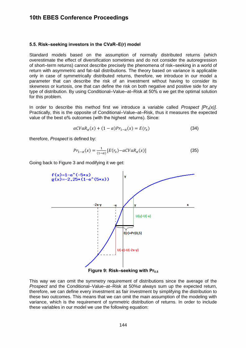
10th EBES Conference Proceedings
144
5.5. Risk–seeking investors in the CVaR–E(r) model Standard models based on the assumption of normally distributed returns (which overestimate the effect of diversification sometimes and do not consider the autoregression of short–term returns) cannot describe precisely the phenomena of risk–seeking in a world of return with asymmetric and fat–tail distributions. The theory based on variance is applicable only in case of symmetrically distributed returns, therefore, we introduce in our model a parameter that can describe the risk of an investment without having to consider its skewness or kurtosis, one that can define the risk on both negative and positive side for any type of distribution. By using Conditional–Value–at–Risk at 50% α we get the optimal solution for this problem. In order to describe this method first we introduce a variable called Prospect [Prα(x)]. Practically, this is the opposite of Conditional–Value–at–Risk, thus it measures the expected value of the best α% outcomes (with the highest returns). Since: (34) therefore, Prospect is defined by:
(35)
Going back to Figure 3 and modifying it we get:
Figure 9: Risk–seeking with Pr0.5
This way we can omit the symmetry requirement of distributions since the average of the Prospect and the Conditional–Value–at–Risk at 50%α always sum up the expected return, therefore, we can define every investment as fair investment by simplifying the distribution to these two outcomes. This means that we can omit the main assumption of the modeling with variance, which is the requirement of symmetric distribution of returns. In order to include these variables in our model we use the following equation:
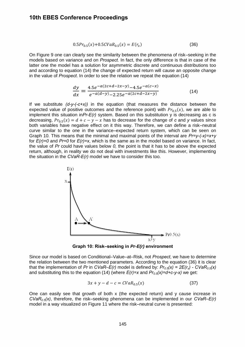
10th EBES Conference Proceedings
145
(36) On Figure 9 one can clearly see the similarity between the phenomena of risk–seeking in the models based on variance and on Prospect. In fact, the only difference is that in case of the latter one the model has a solution for asymmetric discrete and continuous distributions too and according to equation (14) the change of expected return will cause an opposite change in the value of Prospect. In order to see the relation we repeat the equation (14)
(14)
If we substitute (d-y-(-c+x)) in the equation (that measures the distance between the expected value of positive outcomes and the reference point) with , we are able to implement this situation inPr-E(r) system. Based on this substitution y is decreasing as c is decreasing, has to decrease for the change of c and y values since both variables have negative effect on it this way. Therefore, we can define a risk–neutral curve similar to the one in the variance–expected return system, which can be seen on Graph 10. This means that the minimal and maximal points of the interval are Pr=y-(-x)=x+y for E(r)=0 and Pr=0 for E(r)=x, which is the same as in the model based on variance. In fact, the value of Pr could have values below 0, the point is that it has to be above the expected return, although, in reality we do not deal with investments like this. However, implementing the situation in the CVaR-E(r) model we have to consider this too.
Graph 10: Risk–seeking in Pr-E(r) environment
Since our model is based on Conditional–Value–at–Risk, not Prospect, we have to determine the relation between the two mentioned parameters. According to the equation (36) it is clear that the implementation of Pr in CVaR–E(r) model is defined by: Pr0.5(x) = 2E(rx) - CVaR0.5(x) and substituting this to the equation (14) (where E(r)=x and Pr0.5(x)=d+c-y-x) we get: (37)
One can easily see that growth of both x (the expected return) and y cause increase in CVaR0.5(x), therefore, the risk–seeking phenomena can be implemented in our CVaR–E(r) model in a way visualized on Figure 11 where the risk–neutral curve is presented:
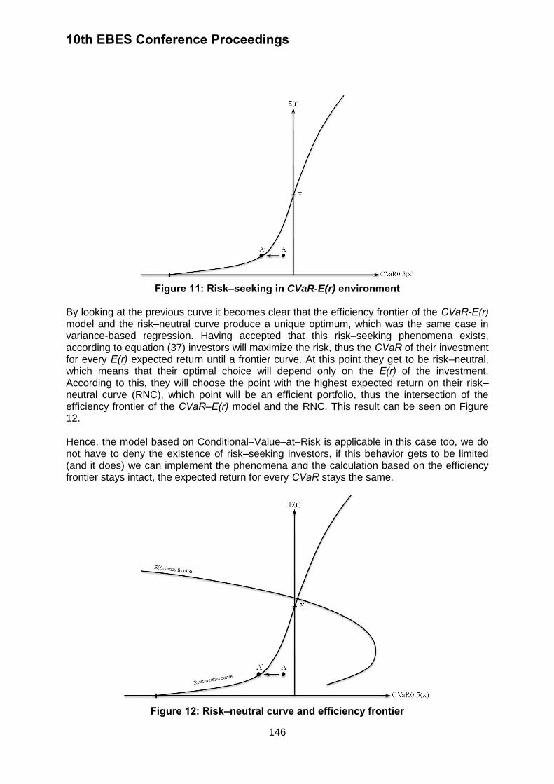
10th EBES Conference Proceedings
146
Figure 11: Risk–seeking in CVaR-E(r) environment
By looking at the previous curve it becomes clear that the efficiency frontier of the CVaR-E(r) model and the risk–neutral curve produce a unique optimum, which was the same case in variance-based regression. Having accepted that this risk–seeking phenomena exists, according to equation (37) investors will maximize the risk, thus the CVaR of their investment for every E(r) expected return until a frontier curve. At this point they get to be risk–neutral, which means that their optimal choice will depend only on the E(r) of the investment. According to this, they will choose the point with the highest expected return on their risk–neutral curve (RNC), which point will be an efficient portfolio, thus the intersection of the efficiency frontier of the CVaR–E(r) model and the RNC. This result can be seen on Figure 12. Hence, the model based on Conditional–Value–at–Risk is applicable in this case too, we do not have to deny the existence of risk–seeking investors, if this behavior gets to be limited (and it does) we can implement the phenomena and the calculation based on the efficiency frontier stays intact, the expected return for every CVaR stays the same.
Figure 12: Risk–neutral curve and efficiency frontier

10th EBES Conference Proceedings
147
6. THE EFFECT OF LIMITED BORROWINGS In this section we omit one of the main, although very unrealistic assumptions of standard asset pricing models, the unlimited borrowings. Equilibrium models define the capital market line (CML) as the set of efficient investment opportunities including risk–free and risky assets that goes to infinity. However, in reality this is not true. In most of the cases there is no opportunity to invest in such positions. Through our model one can calculate the expected return of levered portfolios but by using realistic factors the result is completely different from that of standard regressions. We use non–infinite borrowingconstraint that is available not only for risk–free interest rate. In order to create a leveraged model we make the following assumptions that are much more realistic than the ones used in standard regressions:
For each investor borrowing is limited (no matter it is due to investment credit or short sales). In the followings this is measured by (1+x) (for example in case of 2:1 leverage x=1).
Every time investors use leverage the lending institution defines a margin that involves automatically closing the position or liquidation if the value of portfolio reaches its m percentage. Analytically this means that the return (loss) gets to be equal to the (-1+f) loss, therefore, r=(-1+f).
These assumptions cause investors gaining other advantages in exchange for paying interest rate: on one hand they get insurance "for free" due to liquidation at margin call. In this case the investor cannot lose more than its own invested money, however it would be possible through a leveraged portfolio without marginal requirements. This reduction of risk has no excess cost for him or her, however, he or she gets some of the negative risk eliminated, thus gets higher expected return. This is described on Figure 13 and in the following analytics.
Figure 13: Effect of leverage with marginal requirements
(3)
(4) where:
is the expected return of L leveraged portfoliowith margin requirements
is the expected return of P unleveraged portfolio
is the leverage
is the interest rate for borrowing multiplied by the borrowed quantity (the total cost of borrowing)
is the probability of Q leveraged portfolio without margin
requirements generates return below (-1+f)

10th EBES Conference Proceedings
148
is the Conditional–Value–at–Risk of Q portfolioat p probability
is the Value–at–Risk of Q portfolio at p probability
Since CVaR≥VaR is always true for fix probability distribution and level and rQ gets multiplied by (1+x) for x leverage, therefore, we get increasing marginal expected return in case of margin requirements instead of constant marginal expected return. This means that the relation between the leverage of the portfolio and the expected return is not linear, in the
function describing CVaR-E(r) leveraged portfolios
is not constant.
According to this deduction, it is clear that one can create the following leveraged position: if A and B are unleveraged portfolios, CVaR0.5;A=CVaR0.5;B and E(r)A>E(r)B, A is "more efficient", therefore, it is the optimal choice. However, the reduction effect of margin requirements can have the opposite result for leveraged expected returns if A and B have different probability distributions. This causes E(r)L;A<E(r)L;B if the return of portfolio B has more like fat–tail distribution:
1+ , <−1+ − 1+ , <−1+ >[ ( ) − ( ) ](1+ ) (5)
where rB(1+x) is the leveraged expected return of portfolio B with (1+x) leverage and without including margin requirements; we used the same logic for the other parameters too. The situation mentioned above is presented on Figure 14 where A and B are the portfolios without leverage, A' and B' are the portfolios with (1+x) leverage, D is the interest rate paid for borrowing and the 45° dashed line signs the frontier that no portfolio can exist below since CVaR0.5 ≤ E(r).
Figure 14: Effect of different probability distributions on portfolios
A’
D
CVaR 0.5(x)
E(r)
A
B
B’
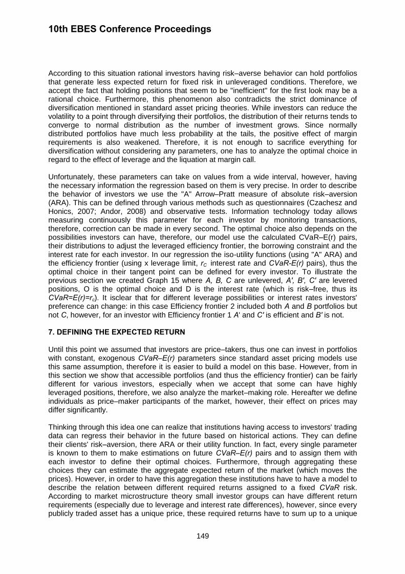
10th EBES Conference Proceedings
149
According to this situation rational investors having risk–averse behavior can hold portfolios that generate less expected return for fixed risk in unleveraged conditions. Therefore, we accept the fact that holding positions that seem to be "inefficient" for the first look may be a rational choice. Furthermore, this phenomenon also contradicts the strict dominance of diversification mentioned in standard asset pricing theories. While investors can reduce the volatility to a point through diversifying their portfolios, the distribution of their returns tends to converge to normal distribution as the number of investment grows. Since normally distributed portfolios have much less probability at the tails, the positive effect of margin requirements is also weakened. Therefore, it is not enough to sacrifice everything for diversification without considering any parameters, one has to analyze the optimal choice in regard to the effect of leverage and the liquation at margin call. Unfortunately, these parameters can take on values from a wide interval, however, having the necessary information the regression based on them is very precise. In order to describe the behavior of investors we use the "A" Arrow–Pratt measure of absolute risk–aversion (ARA). This can be defined through various methods such as questionnaires (Czachesz and Honics, 2007; Andor, 2008) and observative tests. Information technology today allows measuring continuously this parameter for each investor by monitoring transactions, therefore, correction can be made in every second. The optimal choice also depends on the possibilities investors can have, therefore, our model use the calculated CVaR–E(r) pairs, their distributions to adjust the leveraged efficiency frontier, the borrowing constraint and the interest rate for each investor. In our regression the iso-utility functions (using "A" ARA) and the efficiency frontier (using x leverage limit, rC interest rate and CVaR-E(r) pairs), thus the optimal choice in their tangent point can be defined for every investor. To illustrate the previous section we created Graph 15 where A, B, C are unlevered, A', B', C' are levered positions, O is the optimal choice and D is the interest rate (which is risk–free, thus its CVaR=E(r)=rc). It isclear that for different leverage possibilities or interest rates investors' preference can change: in this case Efficiency frontier 2 included both A and B portfolios but not C, however, for an investor with Efficiency frontier 1 A' and C' is efficient and B' is not. 7. DEFINING THE EXPECTED RETURN Until this point we assumed that investors are price–takers, thus one can invest in portfolios with constant, exogenous CVaR–E(r) parameters since standard asset pricing models use this same assumption, therefore it is easier to build a model on this base. However, from in this section we show that accessible portfolios (and thus the efficiency frontier) can be fairly different for various investors, especially when we accept that some can have highly leveraged positions, therefore, we also analyze the market–making role. Hereafter we define individuals as price–maker participants of the market, however, their effect on prices may differ significantly. Thinking through this idea one can realize that institutions having access to investors' trading data can regress their behavior in the future based on historical actions. They can define their clients' risk–aversion, there ARA or their utility function. In fact, every single parameter is known to them to make estimations on future CVaR–E(r) pairs and to assign them with each investor to define their optimal choices. Furthermore, through aggregating these choices they can estimate the aggregate expected return of the market (which moves the prices). However, in order to have this aggregation these institutions have to have a model to describe the relation between different required returns assigned to a fixed CVaR risk. According to market microstructure theory small investor groups can have different return requirements (especially due to leverage and interest rate differences), however, since every publicly traded asset has a unique price, these required returns have to sum up to a unique

10th EBES Conference Proceedings
150
expected return based on some function. Although the purpose of this paper is not defining this precise function, in order to approximate a regression we use the value–weighted aggregating function. This means that we sum up each investor's required return with weights equal to their invested value, thus we get a unique expected return.
Figure 15: Individual optimization with leverage constraints
This weighted aggregation function is based on macroeconomic demand and supply functions. Then the price assigned to a portfolio is defined by the current aggregated supply and demand on the investment opportunity. Since databases allow us analyzing who wants to make transactions on the current price with what volume and what is the required return of the investor, one can define the future price (current price multiplied by the required return) and the future volume of each investor. This way the aggregated supply (AS) function can be defined. According to behavioral financial studies (Fama, 1991) the investors insist on smoothing their consumption over time, therefore, it seems to be realistic to assume that their incoming cash–flows are balanced and continuous due to diversification. Furthermore, if the future cash–flows are assumed to be fixed (which seems to be true since the price always reflects all the information about them), the aggregated demand (AD) grows in the same pace as AS, which is the required return of investors. This means that in the discounted cash–flow pricing method the exponent of the cost of alternative choice is getting smaller over time. Combining the functions mentioned above we create the AS–AD system in our model, hence one can make approximation of future prices of assets and their expected returns. The illustration of this approximation is shown on Figure 16, where the initial (t0) AS and AD functions are increased by continuous return over time (represented on axis "t"). The
D
CVaR 0,5(x)
E(r)
B’
B C
C’
A
A’
O
rC
Isoutility curve
Efficiency frontier 1
Efficiency frontier 2

10th EBES Conference Proceedings
151
functions used are PS=2Q and PD=5-2Q. We fixed the continuous return at fixed 20% in order to be expressive, hence the exponential growth over time can be clearly seen.
Figure 16: The formation of the expected return
We underline that this type of approximation of the expected return is very sensitive to the input data, therefore, the bigger the used database is the more precise the regression will be. This necessary data can be extracted by analyzing the actions of clients in financial institutions or brokerage services, however, using our model at national level (such as under the supervision of the Securities and Exchange Commission) or at international level (for example with the administration of the International Monetary Fund (IMF) or the European Central Bank (ECB)) could produce fairly precise approximations of future prices of capital markets. 8. CONCLUSION The use of Conditional–Value–at–Risk in asset pricing modeling seems to be more and more important since it is a much more precise measure than volatility or standard Value–at–Risk, which can be seen in many recent papers of international financial institutions (for example the recommendation of using CVaR of the Bank for International Settlements (BIS), 2012). Although there have been some model based on this risk measure before our research, they all have used the unrealistic assumptions of the exclusion of risk–seeking or price–maker investors and the infinite borrowing opportunity. Our model has achieved to omit these assumptions, therefore, we could create a more general and realistic regression. The implementation of main utility functions (the one from Expected Utility Theory and the other from Prospect Theory) in CVaR–E(r) system allows defining the optimal choice of each individual in both risk–averse and risk–seeking situations. The inclusion of risk–seeking investors through the Kahneman and Tversky utility function has allowed omitting the first unrealistic assumption of standard models. The price–maker activity described by aggregated demand and supply functions has made the second assumption unnecessary. Although these functions have not been analyzed in this paper, there have numerous attempts to describe them with market microstructural (Biais et al. 2002) or behavioral financial approaches, however, these theories focus on the short–term changes of prices, while on long–term the approximation of expected return through aggregation described in this paper seems to work well in practice. Finally, the third unrealistic assumption (unlimited borrowing for fixed risk–free rate) has become unnecessary too since in our model we define different leverage limit and interest rate for every individual.
10th EBES Conference Proceedings
152
Hence, our asset pricing method can define the required return and the optimal choice for each investor and under proper infrastructural conditions it can aid raising capital for companies through choosing the adequate investors, it supports individuals in trading, makes corporate financial analysis more precise (Andor and Dulk, 2013) and approximates the expected returns and asset prices without using unrealistic assumptions and limitations. REFERENCES Andor, Gy., 2008. Business economics. Budapest: Typotex Press Andor, Gy., and Dulk, M., 2013. Harmonic mean as an approximation for discounting intraperiod cash flows, The Engineering Economist, (forthcoming). Ariely, D., Loewenstein, G., and Prelec, D. 2003. Coherent arbitrariness: Stable demand curves without stable preferences. The Quarterly Journal of Economics, 118(1), pp. 73-106. Bank for International Settlements, 2012. Consultative document: Fundamental review of the trading book. Basel: Bank for International Settlements Biais, B., Glosten, L., and Spatt, C., 2002. The microstructure of stock markets, Discussion Paper No. 3288., London: Centre for Economic Policy Research Campbell, R., Huisman, R., and Koedijk, K., 2001. Optimal portfolio selection in a Value-at-Risk framework. Journal of Banking & Finance, 25(9), pp.1789-1804. Czachesz G. and Honics I., 2007. Measuring the Hungarian investors' risk appetite, Credit Institutes' Review, 6(2), pp.129-166. Erdos, P., Ormos, and M., Zibriczky, D., 2011. Non-parametric and semi-parametric asset pricing, Economic Modelling, 28(3), pp.1150-1162. Erdos, P., Ormos, M., Zibriczky, D., 2010. Is CAPM's characteristic, security-market line a straight one? Economic Review, 57(1), pp.201-221. Fama, E.F., 1991. Efficient capital markets: II, Journal of Finance, 46(5), pp.1575-1617. Gossen, H.H., 1854. The Laws of human relations and the rules of human action derived therefrom. Translated by R.C.Blitz, 1983. Cambridge: The MIT Press Holton, G.A., 2003. Value-at-Risk, San Diego: Academic Press. Jorion, P., 2007. Financial risk manager handbook. Hoboken: John Wiley & Sons. Kahneman, D. and Tversky, A., 1979. Prospect theory: An analysis of decision under risk. Econometrica, 47(2), pp.263-291 Krokhmal, P., Palmquist, J., and Uryasev, S., 2002. Portfolio optimization with conditional Value-at-Risk objective and constraints. Journal of Risk, 4(2), pp.43-48. Lintner, J., 1965. The Valuation of risky assets and the selection of risky investments in stock portfolios and capital budgets. Review of Economics and Statistics, 47(1), pp.13-37.

10th EBES Conference Proceedings
153
Markowitz, H., 1959. Portfolio selection. New Haven: Yale University Press. Meng, Z., Jiang, M., and Hu, Q., 2011. Dynamic CVaR with multi-period risk problems. Journal of System Science and Complexity, 24(5), pp.907-918. Mossin, J., 1966. Equilibrium in a capital asset market. Econometrica, 34(4) pp.768-783 Pratt, J.W., 1964. Risk aversion in the small and in the large. Econometrica, 32(1/2), pp.122-136 Rockafellar, R.T. and Uryasev, S., 2000. Optimization of conditional value-at-risk. Journal of Risk, 2(3), pp.21–41. Rockafellar, R.T. and Uryasev, S., 2002. Conditional value-at-risk for general loss distributions, Journal of Banking & Finance, 26(7), pp. 1443-1471. Sharpe, W.F., 1964. Capital asset prices: A theory of market equilibrium under conditions of risk. Journal of Finance, 19(3), pp.425-442. Shefrin, H., 2002. Beyond greed and fear, Oxford: Oxford University Press Thaler, R.H. and Johnson, E.J., 1990. Gambling with the house money and trying to break even: The effects of prior outcomes on risky choice. Management Science, 36(6), pp.643-60. Timotity, D., 2012. Risk without limits, Students' Science Conference, Budapest, Hungary 14 November 2012. Budapest: Budapest University of Technology and Economics

10th EBES Conference Proceedings 23 - 25 May, 2013. NIPPON HOTEL, ISTANBUL, TURKEY ISBN: 978-605-64002-1-6. WEBSITE: www.ebesweb.org
154
CULTURAL OPENNESS AS A FACTOR OF BUILDING CREATIVE REGION: WROCLAW COMPARED TO OTHER
POLISH CITIES
MALGORZATA NIKLEWICZ-PIJACZYNSKA Faculty of Law, Administration and Economics
University of Wroclaw Poland
MALGORZATA WACHOWSKA Faculty of Law, Administration and Economics
University of Wroclaw Poland
[email protected] Abstract: The article discusses impact of openness on economic development of regions. As a basis for discussion has been adopted Richard Florida’s 3T theory, according to which tolerance or otherwise region openness to diversity and otherness is one of elements (in addition to talent and technology), which promotes creativity, and ultimately economic success. The purpose of this article is to examine Wroclaw city degree of openness. Authorities of Wroclaw have placed R. Florida’s concept as a part of development strategy and are committed to its effective implementation. The openness was evaluated on basis of primary research - surveys of selected groups of respondents, which made possible to determine openness of Wroclaw residents on immigrant population - foreigners and people arriving to the city from other Polish regions. On the basis of research it can be concluded that residents of Wroclaw are open to foreigners, including those who profess a different religion, and have a different skin color as well as people flowing into the city from other parts of the country. This is confirmed by opinions of foreigners living in Wroclaw, as well as speech, gestures and behavior of Wroclaw people. Keywords: Tolerance, Regional Development, Creative Region 1. INTRODUCTION Regional development is commonly associated with economic categories. References are made to micro-and macro-economic drivers of region development. The former have a direct impact on company productivity and can include, among others, quantity and quality of staff training or number of institutions supporting innovativeness. The macroeconomic factors include, in turn, monetary and fiscal policy or social infrastructure. Among the most important drivers of regional development are increasingly pointed out so-called talent or human capital (individual holding a large pool of knowledge, an educated individual), and creative capital (individual showing their creativity, i.e. capable to transform their knowledge into a new idea). However, there lacks the agreement in relation to factors affecting geographic distribution of talent. Usually, among factors that stimulate creativity and attract talented individuals to a region, first mentioned are these representing area of economic incentives, such as educational system and expenditures on education, as well as support for scientists and attractive jobs in

10th EBES Conference Proceedings
155
the region. To a lesser extent, creativity and ability to attract creative individuals are identified with non-economic factors, but in this case one could find the view - especially as far as literature in areas of psychology and sociology is concerned - that creativity is influenced by socio-psychological factors. In studies related to psychology of creativity, it is often connected with tolerance. It is believed that somebody being tolerant, open to change, new ideas and other cultures has greater potential to be creative, because they will also be open to all hypotheses, even those considered to be the most absurd, and so "there is nothing impossible for them". Development of the idea of connecting creativity/talent with openness (tolerance) on the basis of economics is the concept of Florida's 3T (Florida, 2002b), in the light of which, region's openness or tolerance of its people to all otherness, diversity, fosters development of diversity in the sense that it attracts creative capital (creative people, talent), created - according to Florida - mainly by scientists, engineers, computer scientists, architects, designers and people working in education and entertainment, artists and musicians. According to Florida (Florida, 2002b) creative individuals themselves are open and they expect openness from their milieu. Therefore, when deciding where to live, they check whether a region has a high rate of tolerance. If people living in the region are tolerant to gays, bohemians and immigrants (Florida, 2002b), it can be assumed that they are also open to any other differences, including to creative people who - according to Florida - are often characterized by some "quirks" or unconventional manner. Florida verified his theoretical concept empirically basing on example of United States regions (Florida, 2002a, 2002b), indicating that tolerant regions are more effective in attracting creative class. Then, repeating research (2001-2006) for US, he confirmed that geographic distribution of creative capital depends on openness, but in this case, only tolerance to gays and bohemians counted, while tolerance to visible immigrants minority was negatively correlated with talent (Florida et al. 2008). Analysis of Canadian regions over the same period (2001-2006) brought similar results to those from the United States of America (Florida et al. 2010), i.e. openness of Canadian gay and bohemian communities was a magnet for attracting talent, but no correlation has been found between tolerance towards immigrants and talent. In addition, openness as a factor in attracting creative class to Canadian regions has played a greater role than universities and facilities. Importance of openness to regional development through its impact on creative individuals has also been confirmed in Sweden, but in this case, geographic distribution of talent to a greater extent depended on the region's universities and facilities (Mellander, Florida, 2011). Taking into account relationship between tolerance and talent, results obtained in research on Swedish regions are similar to those from Chinese regions (Florida et al. 2012). Here, too, openness of a region had an impact on attracting creative capital, but the key to geographic distribution of talent were universities. Since the openness of a region - by acting on creative class - can be significant for its creativity and, consequently, development, the aim of the paper is to assess Wroclaw inhabitants’ tolerance (Wroclaw is a capital of Lower Silesia region, Poland), especially towards foreigners, immigrants and gays. Indication of the extent to which Wroclaw people are tolerant towards all manner of difference and diversity will help determine the potential of Wroclaw to attract the most talented individuals, and thus indirectly its potential for growth. Of course, region openness is not the only determining factor in its choice by creative individuals, but - as mentioned earlier - results of several researches suggest a significant role of tolerance in attracting creative capital.
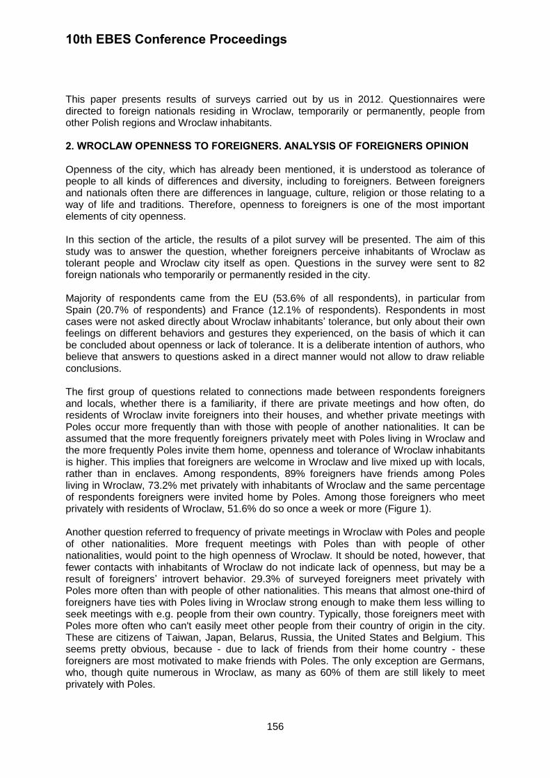
10th EBES Conference Proceedings
156
This paper presents results of surveys carried out by us in 2012. Questionnaires were directed to foreign nationals residing in Wroclaw, temporarily or permanently, people from other Polish regions and Wroclaw inhabitants. 2. WROCLAW OPENNESS TO FOREIGNERS. ANALYSIS OF FOREIGNERS OPINION Openness of the city, which has already been mentioned, it is understood as tolerance of people to all kinds of differences and diversity, including to foreigners. Between foreigners and nationals often there are differences in language, culture, religion or those relating to a way of life and traditions. Therefore, openness to foreigners is one of the most important elements of city openness. In this section of the article, the results of a pilot survey will be presented. The aim of this study was to answer the question, whether foreigners perceive inhabitants of Wroclaw as tolerant people and Wroclaw city itself as open. Questions in the survey were sent to 82 foreign nationals who temporarily or permanently resided in the city. Majority of respondents came from the EU (53.6% of all respondents), in particular from Spain (20.7% of respondents) and France (12.1% of respondents). Respondents in most cases were not asked directly about Wroclaw inhabitants’ tolerance, but only about their own feelings on different behaviors and gestures they experienced, on the basis of which it can be concluded about openness or lack of tolerance. It is a deliberate intention of authors, who believe that answers to questions asked in a direct manner would not allow to draw reliable conclusions. The first group of questions related to connections made between respondents foreigners and locals, whether there is a familiarity, if there are private meetings and how often, do residents of Wroclaw invite foreigners into their houses, and whether private meetings with Poles occur more frequently than with those with people of another nationalities. It can be assumed that the more frequently foreigners privately meet with Poles living in Wroclaw and the more frequently Poles invite them home, openness and tolerance of Wroclaw inhabitants is higher. This implies that foreigners are welcome in Wroclaw and live mixed up with locals, rather than in enclaves. Among respondents, 89% foreigners have friends among Poles living in Wroclaw, 73.2% met privately with inhabitants of Wroclaw and the same percentage of respondents foreigners were invited home by Poles. Among those foreigners who meet privately with residents of Wroclaw, 51.6% do so once a week or more (Figure 1). Another question referred to frequency of private meetings in Wroclaw with Poles and people of other nationalities. More frequent meetings with Poles than with people of other nationalities, would point to the high openness of Wroclaw. It should be noted, however, that fewer contacts with inhabitants of Wroclaw do not indicate lack of openness, but may be a result of foreigners’ introvert behavior. 29.3% of surveyed foreigners meet privately with Poles more often than with people of other nationalities. This means that almost one-third of foreigners have ties with Poles living in Wroclaw strong enough to make them less willing to seek meetings with e.g. people from their own country. Typically, those foreigners meet with Poles more often who can't easily meet other people from their country of origin in the city. These are citizens of Taiwan, Japan, Belarus, Russia, the United States and Belgium. This seems pretty obvious, because - due to lack of friends from their home country - these foreigners are most motivated to make friends with Poles. The only exception are Germans, who, though quite numerous in Wroclaw, as many as 60% of them are still likely to meet privately with Poles.
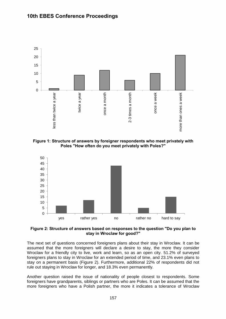
10th EBES Conference Proceedings
157
Figure 1: Structure of answers by foreigner respondents who meet privately with Poles "How often do you meet privately with Poles?"
Figure 2: Structure of answers based on responses to the question "Do you plan to stay in Wroclaw for good?"
The next set of questions concerned foreigners plans about their stay in Wroclaw. It can be assumed that the more foreigners will declare a desire to stay, the more they consider Wroclaw for a friendly city to live, work and learn, so as an open city. 51.2% of surveyed foreigners plans to stay in Wroclaw for an extended period of time, and 23.1% even plans to stay on a permanent basis (Figure 2). Furthermore, additional 22% of respondents did not rule out staying in Wroclaw for longer, and 18.3% even permanently. Another question raised the issue of nationality of people closest to respondents. Some foreigners have grandparents, siblings or partners who are Poles. It can be assumed that the more foreigners who have a Polish partner, the more it indicates a tolerance of Wroclaw
0
5
10
15
20
25
less than t
wic
e a
year
twic
e a
year
once a
month
2-3
tim
es a
month
once a
week
more
than o
nes a
week
0
5
10
15
20
25
30
35
40
45
50
yes rather yes no rather no hard to say

10th EBES Conference Proceedings
158
residents, as they do not close themselves on love relationships with foreigners. Almost 16% of surveyed foreigners are in a partnership with a Pole, but - except one case - men from other countries are involved with Polish women. Another set of questions raised the issue of attitudes to foreign residents of Wroclaw. Respondents were asked in a direct manner if they thought that Wroclaw residents were friendly to them, and whether they met with hostility from the city population, which could be due to non-acceptance of foreigners. 90.2% of all respondents believe that people of Wroclaw refer to them kindly, with friendship. At the same time, 41.5% met with a hostile attitude on the part of Poles, which - in opinion of foreigners - was due to the fact that respondents were foreigners. It should be noted, however, that many respondents note that such events were incidental. Another group of questions were open-ended questions. Foreigners were asked to list three characteristics that they think are the most evident characteristics of Wroclaw residents. This question did not suggest any answers, so it can be assumed that the more spontaneously respondents would determine Wroclaw residents as tolerant/open, the more reasons there are to believe that it is so. 21.9% of respondents identified a Wroclaw resident as tolerant and open to any changes and different cultures. Furthermore, additional 25.6% of respondents found residents of Wroclaw polite, kind and friendly. Although this does not mean exactly what is meant by tolerance, but in this case can be considered as synonymous. It can be therefore concluded that 47.5% of respondents believe that Poles living in Wroclaw are open-minded. However, 7.3% of respondents felt that people of Wroclaw are racists and they are unpleasant, what generally should be regarded as sign of intolerance. Additionally, in a group of open-ended questions were included those checking general knowledge of foreigners about Wroclaw. Having a lot of information about Wroclaw and knowledge of its history suggests that a person is interested in the city that is associated with it and that is involved in life of its inhabitants, which in turn may suggest that the city is an open place. Overall, surveyed foreigners know little about Wroclaw. Most of them know quite well especially those most characteristic places of Wroclaw, and is able to identify various symbols of the city, but only individual persons are able to name cultural events and people involved in Wroclaw. 3. WROCLAW OPENNESS TO INTERNAL IMMIGRATION. RESULTS OF THE SURVEY Questionnaire was addressed to Poles from outside Wroclaw. It involved a group of 128 people who temporarily or permanently reside in Wroclaw, but does not feel to be local1. The largest part of this group were people from cities up to 50 thousand residents (about 39%), followed by rural areas (about 23%) and cities with 50-100 thousand residents. In terms of income, the largest group of respondents were those with net income per household member in the amount of PLN 1000-2000 (about 48%). However, in terms of length of stay, the largest group of respondents were staying in Wroclaw from one to three
1 People who do not come from Wroclaw, but they feel to be local, due to fact of a long time living in the city (for
example, came to Wroclaw in the 50s) were not included in the study, although in many cases based on the fact that they feel home in the city, one could speculate that Wroclaw is very open and its inhabitants are tolerant. Hence, the research group were mainly people up to 39 years of age, as they usually still feel a bond with their native city, even if for some time they already reside in Wroclaw.
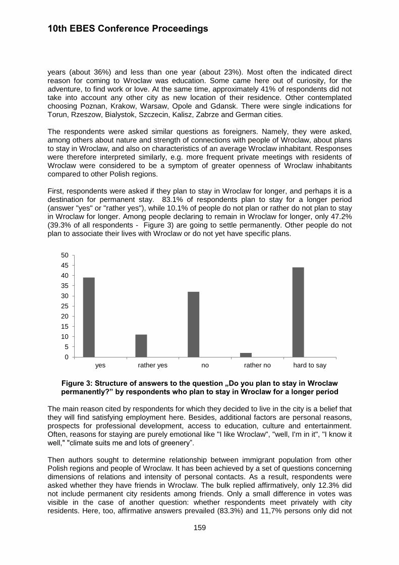
10th EBES Conference Proceedings
159
years (about 36%) and less than one year (about 23%). Most often the indicated direct reason for coming to Wroclaw was education. Some came here out of curiosity, for the adventure, to find work or love. At the same time, approximately 41% of respondents did not take into account any other city as new location of their residence. Other contemplated choosing Poznan, Krakow, Warsaw, Opole and Gdansk. There were single indications for Torun, Rzeszow, Bialystok, Szczecin, Kalisz, Zabrze and German cities. The respondents were asked similar questions as foreigners. Namely, they were asked, among others about nature and strength of connections with people of Wroclaw, about plans to stay in Wroclaw, and also on characteristics of an average Wroclaw inhabitant. Responses were therefore interpreted similarly, e.g. more frequent private meetings with residents of Wroclaw were considered to be a symptom of greater openness of Wroclaw inhabitants compared to other Polish regions. First, respondents were asked if they plan to stay in Wroclaw for longer, and perhaps it is a destination for permanent stay. 83.1% of respondents plan to stay for a longer period (answer "yes" or "rather yes"), while 10.1% of people do not plan or rather do not plan to stay in Wroclaw for longer. Among people declaring to remain in Wroclaw for longer, only 47.2% (39.3% of all respondents - Figure 3) are going to settle permanently. Other people do not plan to associate their lives with Wroclaw or do not yet have specific plans.
Figure 3: Structure of answers to the question „Do you plan to stay in Wroclaw permanently?” by respondents who plan to stay in Wroclaw for a longer period
The main reason cited by respondents for which they decided to live in the city is a belief that they will find satisfying employment here. Besides, additional factors are personal reasons, prospects for professional development, access to education, culture and entertainment. Often, reasons for staying are purely emotional like "I like Wroclaw", "well, I'm in it", "I know it well," "climate suits me and lots of greenery”. Then authors sought to determine relationship between immigrant population from other Polish regions and people of Wroclaw. It has been achieved by a set of questions concerning dimensions of relations and intensity of personal contacts. As a result, respondents were asked whether they have friends in Wroclaw. The bulk replied affirmatively, only 12.3% did not include permanent city residents among friends. Only a small difference in votes was visible in the case of another question: whether respondents meet privately with city residents. Here, too, affirmative answers prevailed (83.3%) and 11,7% persons only did not
0
5
10
15
20
25
30
35
40
45
50
yes rather yes no rather no hard to say
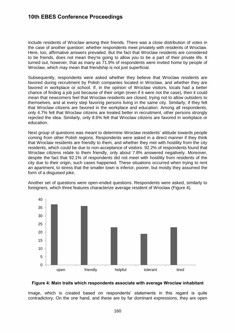
10th EBES Conference Proceedings
160
include residents of Wroclaw among their friends. There was a close distribution of votes in the case of another question: whether respondents meet privately with residents of Wroclaw. Here, too, affirmative answers prevailed. But the fact that Wroclaw residents are considered to be friends, does not mean they're going to allow you to be a part of their private life. It turned out, however, that as many as 71.9% of respondents were invited home by people of Wroclaw, which may mean that friendship is not just superficial. Subsequently, respondents were asked whether they believe that Wroclaw residents are favored during recruitment by Polish companies located in Wroclaw, and whether they are favored in workplace or school. If, in the opinion of Wroclaw visitors, locals had a better chance of finding a job just because of their origin (even if it were not the case), then it could mean that newcomers feel that Wroclaw residents are closed, trying not to allow outsiders to themselves, and at every step favoring persons living in the same city. Similarly, if they felt that Wroclaw citizens are favored in the workplace and education. Among all respondents, only 4.7% felt that Wroclaw citizens are treated better in recruitment, other persons strongly rejected the idea. Similarly, only 8.6% felt that Wroclaw citizens are favored in workplace or education. Next group of questions was meant to determine Wroclaw residents’ attitude towards people coming from other Polish regions. Respondents were asked in a direct manner if they think that Wroclaw residents are friendly to them, and whether they met with hostility from the city residents, which could be due to non-acceptance of visitors. 92.2% of respondents found that Wroclaw citizens relate to them friendly, only about 7.8% answered negatively. Moreover, despite the fact that 92.1% of respondents did not meet with hostility from residents of the city due to their origin, such cases happened. These situations occurred when trying to rent an apartment, to stress that the smaller town is inferior, poorer, but mostly they assumed the form of a disguised joke. Another set of questions were open-ended questions. Respondents were asked, similarly to foreigners, which three features characterize average resident of Wroclaw (Figure 4).
Figure 4: Main traits which respondents associate with average Wroclaw inhabitant Image, which is created based on respondents’ statements in this regard is quite contradictory. On the one hand, and these are by far dominant expressions, they are open
0
5
10
15
20
25
30
35
40
open friendly helpful tolerant tired
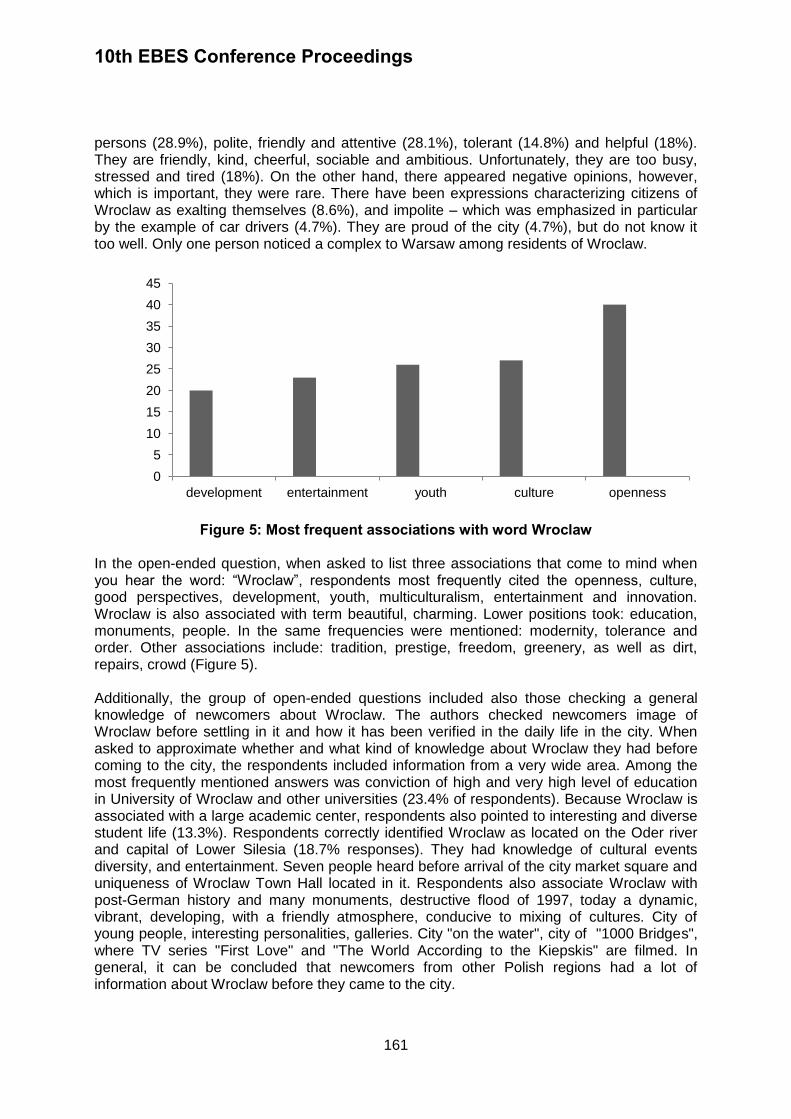
10th EBES Conference Proceedings
161
persons (28.9%), polite, friendly and attentive (28.1%), tolerant (14.8%) and helpful (18%). They are friendly, kind, cheerful, sociable and ambitious. Unfortunately, they are too busy, stressed and tired (18%). On the other hand, there appeared negative opinions, however, which is important, they were rare. There have been expressions characterizing citizens of Wroclaw as exalting themselves (8.6%), and impolite – which was emphasized in particular by the example of car drivers (4.7%). They are proud of the city (4.7%), but do not know it too well. Only one person noticed a complex to Warsaw among residents of Wroclaw.
Figure 5: Most frequent associations with word Wroclaw In the open-ended question, when asked to list three associations that come to mind when you hear the word: “Wroclaw”, respondents most frequently cited the openness, culture, good perspectives, development, youth, multiculturalism, entertainment and innovation. Wroclaw is also associated with term beautiful, charming. Lower positions took: education, monuments, people. In the same frequencies were mentioned: modernity, tolerance and order. Other associations include: tradition, prestige, freedom, greenery, as well as dirt, repairs, crowd (Figure 5). Additionally, the group of open-ended questions included also those checking a general knowledge of newcomers about Wroclaw. The authors checked newcomers image of Wroclaw before settling in it and how it has been verified in the daily life in the city. When asked to approximate whether and what kind of knowledge about Wroclaw they had before coming to the city, the respondents included information from a very wide area. Among the most frequently mentioned answers was conviction of high and very high level of education in University of Wroclaw and other universities (23.4% of respondents). Because Wroclaw is associated with a large academic center, respondents also pointed to interesting and diverse student life (13.3%). Respondents correctly identified Wroclaw as located on the Oder river and capital of Lower Silesia (18.7% responses). They had knowledge of cultural events diversity, and entertainment. Seven people heard before arrival of the city market square and uniqueness of Wroclaw Town Hall located in it. Respondents also associate Wroclaw with post-German history and many monuments, destructive flood of 1997, today a dynamic, vibrant, developing, with a friendly atmosphere, conducive to mixing of cultures. City of young people, interesting personalities, galleries. City "on the water", city of "1000 Bridges", where TV series "First Love" and "The World According to the Kiepskis" are filmed. In general, it can be concluded that newcomers from other Polish regions had a lot of information about Wroclaw before they came to the city.
0
5
10
15
20
25
30
35
40
45
development entertainment youth culture openness

10th EBES Conference Proceedings
162
Then, their knowledge of Wroclaw was enriched during everyday life. The respondents flawlessly mentioned President R. Dutkiewicz as head of the local authority. They also mentioned a beautiful zoo, chess clubs and football club "Śląsk Wroclaw". Then, respondents were asked what socio-cultural initiatives associated with Wroclaw they knew. It turned out that best known initiatives are Wroclaw - European Capital of Culture and The Meeting Place Wroclaw. Less frequently they mentioned EURO 2012, Review of Stage Songs and the Era New Horizons. 36% do not identify Wroclaw with any socio-cultural initiative. When asked, in turn, about well-known public figures associated with Wroclaw, subjects mentioned above all R. Dutkiewicz, who with 25.8% of votes was far ahead of prof. J. Miodek (8.6% of responses), L. Czarnecki (5.6% of responses) and politicians - G. Schetyna and B. Zdrojewski (each got 4.5% of responses). Those who receive a single vote included M. Krajewski, R. Gonera, W. Frasyniuk and G. Baczynska. However, 36.7% of people do not associate Wroclaw with any public figure. Respondents also tried to indicate places in Wroclaw which were climatic, atmospheric, unique in their opinion Wroclaw. In the ranking of the most magical places decisively won the Cathedral Island. In the second place came Market Square and the island called Wyspa Slodowa. Pergola, Szczytnicki Park and the Japanese Garden remained far behind. When asked to nominate a symbol of the city, respondents clearly pointed to the Town Hall and the Market Square as a whole. Wroclaw dwarfs were in the second place and bridges in the third one. Summary of primary survey results, in which questions were directed at people coming to Wroclaw from other regions of the country, was partly confronted with opinions of Wroclaw residents themselves concerning their tolerance towards people from other places. Namely, Wroclaw residents were asked on three issues. First, they were asked whether they should be favored against people from other Polish cities during recruitment for position in a company located in Wroclaw. For 94 surveyed people, vast majority of respondents (92.5%) answered "no". Then respondents were asked whether it is important for them that their friends were Wroclaw residents. In this regard, vast majority of responses were negative ones (97.8%). Votes on the third issue, however, were distributed very differently, which is whether they internally sympathize with people from Wroclaw. As many as 72.3% of those surveyed answered "yes". This means that while your friends are chosen by a completely different key than urban or regional membership, the inner bond, a sense of belonging, seems to be very strong. 4. ANALYSIS OF WROCLAW RESIDENTS’ OPENNESS, BASED ON THEIR OWN OPINIONS - RESULTS OF PRIMARY STUDIES Another pilot survey, this time conducted among 51 inhabitants of Wroclaw, was designed to determine attitudes of city citizens towards specific groups and communities. Comparison of previous primary studies and the survey presented below serve as a kind of confrontation on how residents of Wroclaw are perceived outside - in other words, what is the commercial image of the city and its inhabitants, with actual attitudes and views of Wroclaw residents.
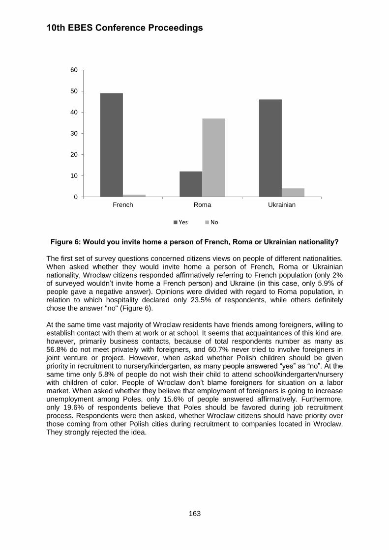
10th EBES Conference Proceedings
163
Figure 6: Would you invite home a person of French, Roma or Ukrainian nationality? The first set of survey questions concerned citizens views on people of different nationalities. When asked whether they would invite home a person of French, Roma or Ukrainian nationality, Wroclaw citizens responded affirmatively referring to French population (only 2% of surveyed wouldn’t invite home a French person) and Ukraine (in this case, only 5.9% of people gave a negative answer). Opinions were divided with regard to Roma population, in relation to which hospitality declared only 23.5% of respondents, while others definitely chose the answer "no" (Figure 6). At the same time vast majority of Wroclaw residents have friends among foreigners, willing to establish contact with them at work or at school. It seems that acquaintances of this kind are, however, primarily business contacts, because of total respondents number as many as 56.8% do not meet privately with foreigners, and 60.7% never tried to involve foreigners in joint venture or project. However, when asked whether Polish children should be given priority in recruitment to nursery/kindergarten, as many people answered “yes” as “no”. At the same time only 5.8% of people do not wish their child to attend school/kindergarten/nursery with children of color. People of Wroclaw don’t blame foreigners for situation on a labor market. When asked whether they believe that employment of foreigners is going to increase unemployment among Poles, only 15.6% of people answered affirmatively. Furthermore, only 19.6% of respondents believe that Poles should be favored during job recruitment process. Respondents were then asked, whether Wroclaw citizens should have priority over those coming from other Polish cities during recruitment to companies located in Wroclaw. They strongly rejected the idea.
0
10
20
30
40
50
60
French Roma Ukrainian
Yes No
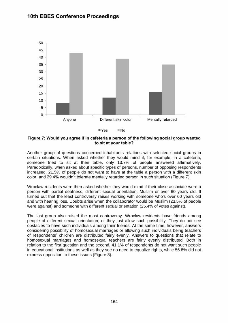
10th EBES Conference Proceedings
164
Figure 7: Would you agree if in cafeteria a person of the following social group wanted
to sit at your table? Another group of questions concerned inhabitants relations with selected social groups in certain situations. When asked whether they would mind if, for example, in a cafeteria, someone tried to sit at their table, only 13.7% of people answered affirmatively. Paradoxically, when asked about specific types of persons, number of opposing respondents increased. 21.5% of people do not want to have at the table a person with a different skin color, and 29.4% wouldn’t tolerate mentally retarded person in such situation (Figure 7). Wroclaw residents were then asked whether they would mind if their close associate were a person with partial deafness, different sexual orientation, Muslim or over 60 years old. It turned out that the least controversy raises working with someone who's over 60 years old and with hearing loss. Doubts arise when the collaborator would be Muslim (23.5% of people were against) and someone with different sexual orientation (25.4% of votes against). The last group also raised the most controversy. Wroclaw residents have friends among people of different sexual orientation, or they just allow such possibility. They do not see obstacles to have such individuals among their friends. At the same time, however, answers considering possibility of homosexual marriages or allowing such individuals being teachers of respondents’ children are distributed fairly evenly. Answers to questions that relate to homosexual marriages and homosexual teachers are fairly evenly distributed. Both in relation to the first question and the second, 41.1% of respondents do not want such people in educational institutions as well as they see no need to equalize rights, while 56.8% did not express opposition to these issues (Figure 8).
0
5
10
15
20
25
30
35
40
45
50
Anyone Different skin color Mentally retarded
Yes No
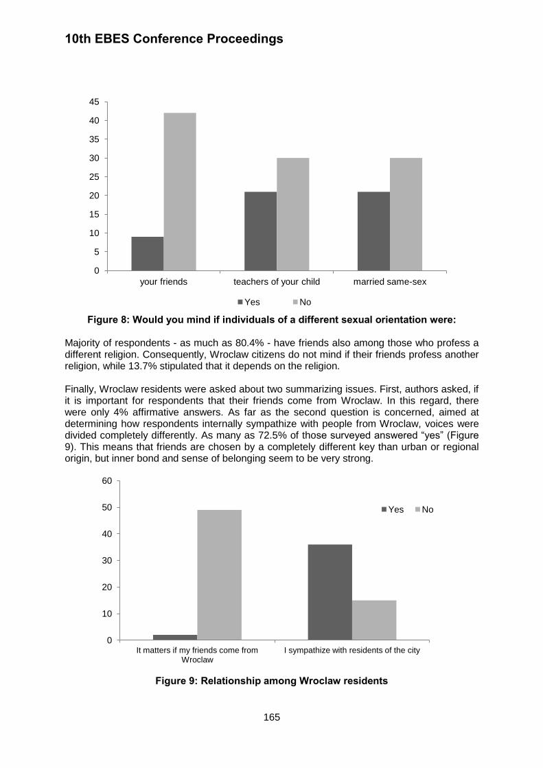
10th EBES Conference Proceedings
165
Figure 8: Would you mind if individuals of a different sexual orientation were:
Majority of respondents - as much as 80.4% - have friends also among those who profess a different religion. Consequently, Wroclaw citizens do not mind if their friends profess another religion, while 13.7% stipulated that it depends on the religion. Finally, Wroclaw residents were asked about two summarizing issues. First, authors asked, if it is important for respondents that their friends come from Wroclaw. In this regard, there were only 4% affirmative answers. As far as the second question is concerned, aimed at determining how respondents internally sympathize with people from Wroclaw, voices were divided completely differently. As many as 72.5% of those surveyed answered “yes” (Figure 9). This means that friends are chosen by a completely different key than urban or regional origin, but inner bond and sense of belonging seem to be very strong.
Figure 9: Relationship among Wroclaw residents
0
5
10
15
20
25
30
35
40
45
your friends teachers of your child married same-sex
Yes No
0
10
20
30
40
50
60
It matters if my friends come from Wroclaw
I sympathize with residents of the city
Yes No
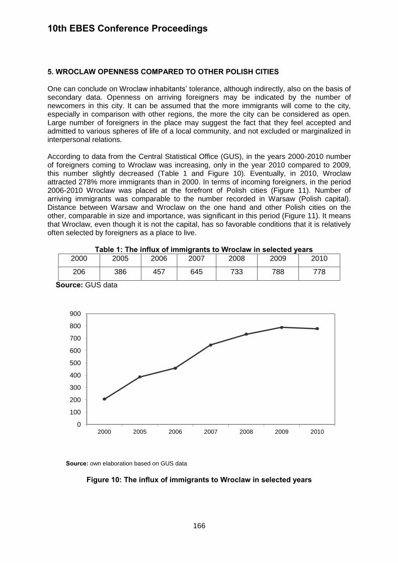
10th EBES Conference Proceedings
166
5. WROCLAW OPENNESS COMPARED TO OTHER POLISH CITIES One can conclude on Wroclaw inhabitants’ tolerance, although indirectly, also on the basis of secondary data. Openness on arriving foreigners may be indicated by the number of newcomers in this city. It can be assumed that the more immigrants will come to the city, especially in comparison with other regions, the more the city can be considered as open. Large number of foreigners in the place may suggest the fact that they feel accepted and admitted to various spheres of life of a local community, and not excluded or marginalized in interpersonal relations. According to data from the Central Statistical Office (GUS), in the years 2000-2010 number of foreigners coming to Wroclaw was increasing, only in the year 2010 compared to 2009, this number slightly decreased (Table 1 and Figure 10). Eventually, in 2010, Wroclaw attracted 278% more immigrants than in 2000. In terms of incoming foreigners, in the period 2006-2010 Wroclaw was placed at the forefront of Polish cities (Figure 11). Number of arriving immigrants was comparable to the number recorded in Warsaw (Polish capital). Distance between Warsaw and Wroclaw on the one hand and other Polish cities on the other, comparable in size and importance, was significant in this period (Figure 11). It means that Wroclaw, even though it is not the capital, has so favorable conditions that it is relatively often selected by foreigners as a place to live.
Table 1: The influx of immigrants to Wroclaw in selected years 2000 2005 2006 2007 2008 2009 2010
206 386 457 645 733 788 778
Source: GUS data
Source: own elaboration based on GUS data
Figure 10: The influx of immigrants to Wroclaw in selected years
0
100
200
300
400
500
600
700
800
900
2000 2005 2006 2007 2008 2009 2010
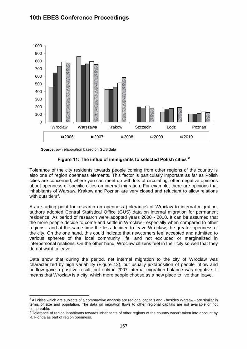
10th EBES Conference Proceedings
167
Source: own elaboration based on GUS data
Figure 11: The influx of immigrants to selected Polish cities 2
Tolerance of the city residents towards people coming from other regions of the country is also one of region openness elements. This factor is particularly important as far as Polish cities are concerned, where you can meet up with lots of circulating, often negative opinions about openness of specific cities on internal migration. For example, there are opinions that inhabitants of Warsaw, Krakow and Poznan are very closed and reluctant to allow relations with outsiders3. As a starting point for research on openness (tolerance) of Wroclaw to internal migration, authors adopted Central Statistical Office (GUS) data on internal migration for permanent residence. As period of research were adopted years 2000 - 2010. It can be assumed that the more people decide to come and settle in Wroclaw - especially when compared to other regions - and at the same time the less decided to leave Wroclaw, the greater openness of the city. On the one hand, this could indicate that newcomers feel accepted and admitted to various spheres of the local community life, and not excluded or marginalized in interpersonal relations. On the other hand, Wroclaw citizens feel in their city so well that they do not want to leave. Data show that during the period, net internal migration to the city of Wroclaw was characterized by high variability (Figure 12), but usually juxtaposition of people inflow and outflow gave a positive result, but only in 2007 internal migration balance was negative. It means that Wroclaw is a city, which more people choose as a new place to live than leave.
2 All cities which are subjects of a comparative analysis are regional capitals and - besides Warsaw - are similar in
terms of size and population. The data on migration flows to other regional capitals are not available or not comparable. 3 Tolerance of region inhabitants towards inhabitants of other regions of the country wasn't taken into account by
R. Florida as part of region openness.
0
100
200
300
400
500
600
700
800
900
1000
Wroclaw Warszawa Krakow Szczecin Lodz Poznan
2006 2007 2008 2009 2010
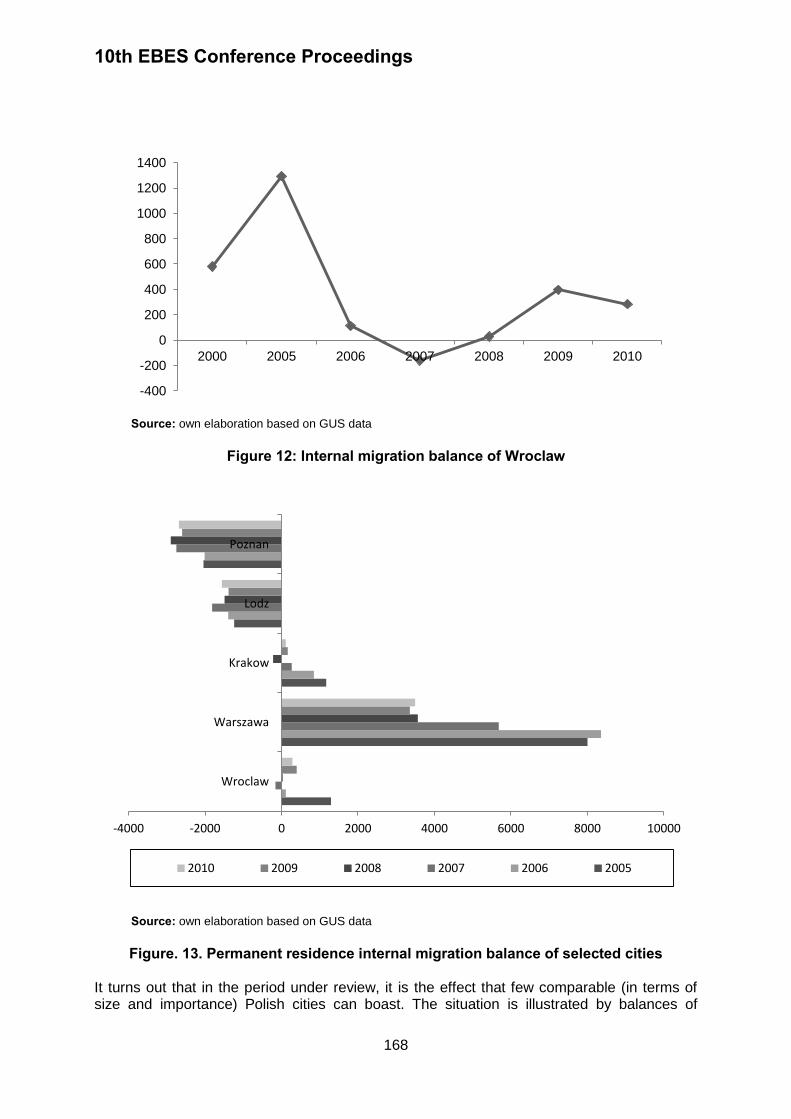
10th EBES Conference Proceedings
168
Source: own elaboration based on GUS data
Figure 12: Internal migration balance of Wroclaw
Source: own elaboration based on GUS data
Figure. 13. Permanent residence internal migration balance of selected cities
It turns out that in the period under review, it is the effect that few comparable (in terms of size and importance) Polish cities can boast. The situation is illustrated by balances of
-400
-200
0
200
400
600
800
1000
1200
1400
2000 2005 2006 2007 2008 2009 2010
-4000 -2000 0 2000 4000 6000 8000 10000
Wroclaw
Warszawa
Krakow
Lodz
Poznan
2010 2009 2008 2007 2006 2005

10th EBES Conference Proceedings
169
internal migration for Wroclaw, Warsaw, Krakow, Lodz, and Poznan (Figure 13). As it is clear from the juxtaposition, Wroclaw is among cities that since 2005 record in most cases positive net internal migration. Only Warsaw and Krakow can still boast such a result. In Poznan and Lodz, starting from 2005, net migration has negative values, which literally means that more people are choosing to move out of them than to live in them. 6. CONCLUSIONS Literature in area of psychology emphasizes that a tolerant person, open to change, new ideas and different cultures has the potential for being creative. This is mainly due to fact that such individuals are also open to all hypotheses, even those considered to be the most absurd, and thus "there is nothing impossible for them." An extension of this idea on economic basis is, among others, R. Florida's 3T theory, according to which tolerance or openness of the region to dissidence and diversity fosters creativity in the sense that it attracts creative people. Wroclaw authorities’ conviction of existence of relationships between tolerance and regional development described by Florida, makes their efforts aimed at creating and strengthening city's image as an open one. In part, this is a successful strategy. This is indicated by analysis of primary data collected during the pilot study. This article focuses mainly on examination of Wroclaw inhabitants’ openness towards foreigners and people coming from other Polish regions. To a lesser extent, Wroclaw residents’ tolerance for people of different sexual orientation was examined. Inclusion of openness to people from other regions is very important in assessing tolerance of a Polish region. In the authors’ opinion, it is possible to meet above-mentioned symptoms of discrimination against that group of people in Poland. Based on the analysis carried out in the article, it can be assumed that people of Wroclaw are open to foreigners, including those who profess a different religion and have a different skin color. It is evidenced by statistical data, opinions of foreigners living in Wroclaw as well as opinions, actions and behavior of Wroclaw residents (although to lesser extent). Also, based on the opinion of foreigners themselves, it can be concluded that residents of Wroclaw are open to foreigners. Evidenced by the fact that vast majority (73%) of surveyed foreigners (who adhere to a different religion and have a different skin color) meet privately in Poland with Wroclaw residents, including at their homes. Moreover, in most cases (51%) these contacts occur relatively frequently, once a week or more. And most importantly, as much as 90% of respondents foreigners believe that Wroclaw residents refer to them with kindness and friendship. These conclusions are reinforced by fact that 16% of respondents are in close personal relations with Poles, 22% (answering the open-ended question) identified Wroclaw inhabitant as tolerant and open to any changes and culture, and 29% meet privately more frequently with Poles than people of other nationalities. In all these cases, above results should be regarded as high score. Being in personal relationship with foreigner means admission into most intimate spheres of Wroclaw inhabitant’s life. However, spontaneous determination of Wroclaw inhabitant as open minded in the question which should indicate three characteristics of average city inhabitant also largely indicates tolerance. And finally, more frequent contacts with people of other nationalities are rather rare (regardless of residence country). Wroclaw can be regarded as a city open to foreigners also in opinions of its residents, although in some cases it seems that tolerance is only due to "political correctness." On the

10th EBES Conference Proceedings
170
one hand, Wroclaw citizens are willing to establish contacts with foreigners, and 43% meets with them in private, but on the other hand, not all foreigners are welcome. While 98% of Wroclaw citizens would invite home a person of French nationality and 95% would invite home somebody of Ukrainian nationality, a person of Roma nationality would be welcomed only by 23%. It should be emphasized, however, that despite the crisis, and growing unemployment in Poland, 81% of surveyed Wroclaw residents believe that Poles should not be favored at the time of job recruitment, which to a large extent can be considered as a sign of tolerance. Similarly, as many as 50% of Wroclaw residents believe that Polish children should not be favored in recruitment to nursery, despite the fact that every year, many children fail to qualify for it due to very small number of pre-school institutions. Wroclaw is also a place open to internal migrants. Also, in opinion of those who come to the city, it is considered to be an open city. Almost 40% of all respondents intend to remain in the city on a permanent basis, 87.7% has friends among Wroclaw residents, and consequently meet privately with residents of Wroclaw, including at their homes (72%). In addition, 92.1% of respondents said that Wroclaw citizens relate to them friendly and the same percent did not meet with any hostility on the part of Wroclaw residents. All of these results can be regarded as a sign of openness on the part of the city inhabitants. In addition, visitors showed a great knowledge of Wroclaw: they associate public figures, places, symbols, and socio-cultural initiatives, which suggests that they are emotionally connected with the city, and that they feel good in it. And finally, in an open-ended question, 43.8% of respondents spontaneously identified a Wroclaw resident as open and tolerant person, and in addition 28.1% characterized them as polite, friendly and pleasant, which in this case can also be regarded as a sign of openness. Based on Wroclaw residents’ opinion, the city can be defined as open to internal migrants. 96% of respondents say, it does not matter which Polish city their friend comes from, which means that Wroclaw residents choose friends according to criteria other than nationality or region of origin. In addition, Wroclaw citizens think that when interviewing for job in Wroclaw, in no way they should be privileged, what also testifies to openness. Conclusions of the primary study are strengthened by the secondary one. Statistics show that in years 2000-2010 number of immigrants coming to Wroclaw increased by 278%, and in 2007-2010, Wroclaw and Warsaw (Polish capital) were cities which attracted far more foreigners than other Polish cities. It can be assumed that these trends indicate openness of Wroclaw, as apparently foreigners feel accepted, since they choose the city as place of residence. Such high scores for Wroclaw, as far as number of incoming foreigners is taken into account, could be explained by favorable geographical location and income level of the city (Wroclaw is located in southwestern part of the country – in proximity of other EU countries; belongs to so-called “A Poland”, which is characterized by standard of living and higher incomes of residents than in “B Poland”). However, the capital of Wielkopolska region - Poznan - also has a favorable location and a high income, and yet less foreigners flows to this city. Wroclaw is also a place open to internal migrants. Number of people coming to Wroclaw from other Polish regions in 2010 increased by 45% compared to 2000, and from 2005 to 2010 placed Wroclaw in third place (behind Warsaw and Krakow) in terms of internal migrants coming, but the distance separating it from Krakow was short. Additionally, with one exception, in the period 2005-2010 Wroclaw registered a positive balance of internal migration, which means that more people were coming to it than left the city. Such a good result could still be boasted by Krakow (in one case, a negative balance) and Warsaw (entirely positive balance). Poznan and Lodz permanently showed a negative balance in this
10th EBES Conference Proceedings
171
regard. Wroclaw is not a place open to all social groups. While foreigners and internal migrants can feel accepted, people of different sexual orientation are accepted to a lesser extent (in the light of Wroclaw residents’ own opinions). Although Wroclaw citizens have friends among such people or allow such possibility, 25.4% of respondents wouldn’t want their close associate to be a person of a different sexual orientation, 41.1% would not like such persons to be teachers of their children and the same percent of respondents opposes marriages of the same sex couples. In summary, it is difficult to clearly identify Wroclaw’s degree of openness. If we recognize, like R. Florida, that the most important determinant of tolerance is tolerance towards homosexuals, it would be difficult to consider the city as fully open. It should be noted at this point that the analysis of Wroclaw residents’ openness towards this social group was carried out only on the basis of residents’ opinion, who answered a very limited set of questions about attitudes towards people with different sexual orientation. However, taking into account Wroclaw residents’ openness to foreigners and internal migrants, majority of data and information supports the fact that Wroclaw is an open city, even compared to other Polish cities (of similar size and importance). It can therefore be concluded that Wroclaw has the potential to attract talented individuals, and consequently to the regional development. REFERENCES
Florida, R., 2002a. The economic geography of talent. Annals of the Association of American Geographers, 92(4), pp.743-755.
Florida, R., 2002b. The rise of the creative class. New York: Basic Books.
Florida, R., Mellander, C.P.A., and Stolarick, K.M., 2008. Inside the black box of regional development – human capital, the creative class and tolerance. Journal of Economic Geography, 8(5), pp.615-649.
Florida, R., Mellander, C.P.A., and Stolarick, K.M., 2010. Talent, technology and tolerance in Canadian regional development. Canadian Geographer – Geographe Canadien, 3, pp. 277-304. Florida, R., Mellander, C.P.A., and Qian H.F., 2012. China’s development disconnect. Environment and Planning, 44 (3), pp. 628-648. Mellander, C.P.A. and Florida, R., 2011. Creativity, talent, and regional wages in Sweden. Annals of Regional Science, 46(3), pp.637-660.

10th EBES Conference Proceedings 23 - 25 May, 2013. NIPPON HOTEL, ISTANBUL, TURKEY ISBN: 978-605-64002-1-6. WEBSITE: www.ebesweb.org
172
BUILDING A LEARNING ORGANIZATION: DO LEADERSHIP STYLES MATTER?
NORASHIKIN HUSSEIN
Faculty of Business Management Universiti Teknologi MARA University
Malaysia [email protected]
NOORMALA AMIR ISHAK
Faculty Of Business Management Universiti Teknologi MARA
Malaysia [email protected]
FAUZIAH NOORDIN
Faculty of Business Management Universiti Teknologi MARA
Malaysia [email protected]
Abstract: Many organizations are adopting the strategy of continuous learning to survive and remain competitive in the turbulent business environment. Becoming a learning organization is one of the best ways an organization can improve their services and practices in order to increase their effectiveness and achieve competitive advantage. In this context, the leadership styles of the top management are imperative in facilitating the transition to be a learning organization. The current study attempts to: (1) examine the link between leadership styles (transformational leadership and transactional leadership) and building a learning organization and (2) whether the influence of transformational leadership is stronger than of a transactional type of leadership. The statistical results obtained from 150 manufacturing firms in Malaysia indicate significant positive relationships between transformational leadership and building a learning organization. The findings suggest the leadership style that is characterized by idealized influence, inspirational motivation, intellectual stimulation and individual consideration are important to generate learning in the organization. Keywords: Learning Organization, Leadership Styles, Transformational Leadership 1. INTRODUCTION The competitive pressures of the turbulent business environment have called for the development of a new, improved and effective form of organizations (Gunasekaran, 2004). Singh (2008) highlighted that the existing structure and approaches of organization are not flexible enough to respond effectively hence competitiveness can no longer be achieved with traditional management approaches but need a change in organization and leadership. As the knowledge economy demands quality human resources, the capability of an organization depends on how fast they can transform to be an organization that continuously learns. This has led to the popularity of learning organization which integrates learning and work in order to sustain continuous improvement of the organization (Watkins and Marsick, 1996). In other words, in a learning organization, people are valued, knowledge is used intensively and new

10th EBES Conference Proceedings
173
competencies are sought to better improve the organization. Advocated as an appropriate paradigm in managing all types of organizations, previous studies associated learning organization with positive organizational outcomes such as competitive advantage (e.g., Atak and Erturgut, 2010; Rowden, 2001; Senge, 1990) and improved performance (e.g., Ellinger et al. 2002; Sahaya, 2012; Yeo, 2003). The role of a leader becomes more critical and important as organizations continuously improve and evolve (Nafei et al. 2012). In other words, the motivation to learn may also come from the types of leadership possessed by the top management of the organization. However, the literature rarely addresses the relationship between leadership styles in building a learning organization (Zagorsek et al. 2009) particularly in the Asian context. Furthermore, this issue received minimal attention in the Malaysian context. Thus, it is imperative to explore whether leadership styles matter in building a learning organization. To fill this gap, this study attempts to provide empirical evidence on whether leadership styles of the top management influence the building of learning organization in Malaysia. Specifically this study attempts to answer the following questions: (1) what is the link between leadership styles and building a learning organization?; (2) which leadership style has a stronger influence on building a learning organization? 2. LEARNING ORGANIZATION Scholars and practitioners have shown an increasing interest in the concept of learning organization (Sahaya, 2012). Defined as an organization that inculcates culture and facilitates learning of all its members, learning organization possesses characteristics to meet the ever-changing needs of the environment. The concept of learning organization is most associated with Senge (1990) as a result of his publication The Fifth Discipline: The Art and Practice of the Learning Organization. Senge believed that an affective learning organization is an organization that regenerates itself through learning. According to Senge (1990), there are five components which are essential to a learning organization: shared vision, personal mastery, mental models, team learning and systems thinking. Watkins and Marsick (1997) on the other hand suggest that a learning organization is a constantly learning and transforming organization. Seven imperative actions were identified for a learning organization. Table 1 provides the definition of each of the dimensions of a learning organization. 3. LEADERSHIP STYLES IN BUILDING LEARNING ORGANIZATIONS Leaders especially top management play a very significant role in building high performing organizations. Vision, motivation, systems and structures are provided by leaders at various levels in order to assist organizational learning, thus developing the organization to be a learning organization (Senge, 1990). The concept of transformational-transactional leadership was first articulated by Burns in 1978 and later was modified by Bass (1985). According to Bass (1985), transformational leadership refers to the process of building commitment to the organization’s objectives and empowering followers to accomplish these objectives. The four dimensions that comprise transformational leadership are encouraging subordinates to view problems from new perspectives (intellectual stimulation), provide support and encouragement (individualized consideration), communicate vision (inspirational motivation), and stimulate emotion and identification (idealized influence) (Bass and Avolio, 1995). Transactional leadership on the other hand is based on the exchange on what is required and will reward if the requirements have been fulfilled. Transactional leadership consisted of two dimensions, firstly, contingent reward which referred to as a process where the leader and follower mutually agree role and responsibilities for realizing selected

10th EBES Conference Proceedings
174
objectives and secondly, management by exception (active) and management by exception (passive). The former describes an active leader who seeks for variances from expectations and carries out corrective action when abnormalities are recognized. The passive form explains the inclination to tendency to interfere, often unwillingly, only when particular problems become evident (Bass, 1985).
Table 1: Model of the seven dimensions of the learning organization Dimensions Definition
Create continuous learning Learning is designed into work so that people can learn on the job; opportunities are provided for ongoing education and growth.
Promote inquiry and Dialogue
People gain productive reasoning skills to express their views and the capacity to listen and inquire into the views of others; the culture is changed to support questioning, feedback, and experimentation.
Encourage collaboration and team learning
Work is designed to use groups to access different modes of thinking; groups are expected to learn together and work together; collaboration is valued by the culture and rewarded.
Create systems to capture and share learning
Both high- and low-technology systems to share learning are created and integrated with work; access is provided; systems are maintained.
Empower people toward a collective vision
People are involved in setting, owning, and implementing a joint vision; responsibility is distributed close to decision making so that people are motivated to learn toward what they are held accountable to do.
Connect the organization to its environment
People are helped to see the effect of their work on the entire enterprise; people scan the environment and use information to adjust work practices; the organization is linked to its communities.
Provide strategic leadership for learning
Leaders model, champion, and support learning; leadership uses learning strategically for business results.
Source: Marsick and Watkins (2003)
A few researchers (Abu Daud, 2009; Vera and Crossan, 2004; Zagorsek et al. 2009) have called for an integrative leadership styles to enhance organizational outcome. Transformational-transactional leadership approach has been identified as one of them (Abu Daud, 2009). Previous studies portrayed transformational leaders as individuals that lead to positive organizational outcomes such as enhanced organizational performance (Bass, 1985). Indeed, a few studies such as Singh (2008); and Aragon-Correa et al. (2007) found transformational leadership facilitates learning in organization. However, recently more studies confirmed that not only transformational leadership style lead to building a learning organization, indeed transactional leadership has also influences the building of a learning organization. For example Nafei et al. (2012) revealed both transformational and transactional leadership were related to organizational learning among Saudi Banks in Kingdom of Saudi Arabia. In a study of various organizations in Slovenia, Zagorsek et al. (2009) found that both transformational and transactional leadership styles have a strong impact on organizational learning. Specifically both transformational and transactional leadership demonstrated a strong direct impact on two dimensions of organizational learning namely information acquisition; and behavioral and cognitive changes. However, the direct impact of transactional leadership on behavioral and cognitive changes is even stronger than with transformational leadership. In Lebanon, Angela et al. (2011) who conducted a study on retail sector found that both transformational and transactional leadership styles are positively related to various learning organization dimensions. Their study also confirmed that transformational leaders have more profound influence in cultivating a learning organization environment than transactional leaders do. Therefore it is hypothesized that: H1: There is a positive significant relationship between transformational leadership and learning organization dimensions.
10th EBES Conference Proceedings
175
H2: There is a positive significant relationship between transactional leadership and learning organization dimensions. 4. METHODOLOGY The study used organization as the unit of analysis. Middle managers were chosen as key respondents as they were identified to have an adequate level of involvement with regards to the issues under investigation. A middle manager of each organization was asked to rate the top management’s leadership style and to what extent they practice learning organization in their respective organization. To measure leadership styles, the study adapted Bass and Avolio’s (1995) Multifactor Leadership Questionnaire (MLQ-5x), which is one of the most widely and tested measures to measure transformational and transactional leadership (Amitay et al. 2005; Zagorsek et al. 2009). 32 items were used to represent four dimensions of transformational leadership and two dimensions of transactional leadership. Learning organization was measured using 21 items of Dimensions of Learning Organization Questionnaire (DLOQ) developed by Watkins and Marsick (1996). Previous research has established sufficient reliability levels for all scales, and both the content and construct validity of the DLOQ have been confirmed (Yang, 2003). All items in the questionnaire were presented using seven-point Likert Scale from scale ranging from 1 = “Strongly disagree” to 7 = “Strongly agree”. Prior to the study, the questionnaire underwent a pilot test with 30 managers from three manufacturing organizations. Based on the feedbacks obtained, minor modifications were made and the questionnaires were then ready to be distributed. In order to obtain information, personal requests to conduct the survey were made to each manufacturing organization. This sector was chosen for our study because manufacturing organizations operate in an increasingly complex setting (Challis et al. 2005). In order to survive, organizations need to improve their performance through learning and manufacturing organizations are no exception. Indeed, there is a call on ‘learning factory’ recently to indicate that not only service organizations need to learn continuously but manufacturing organizations as well. An exploratory study conducted by Norashikin et al. (2009) indicated that manufacturing organizations in Malaysia were still new in the learning organization approach but they are definitely moving towards it. Using a random sampling method, 547 organizations were contacted but only 150 manufacturing organizations replied and indicated their interest to participate in the study. Questionnaires were then mailed to the respective participating organizations. Upon completion, the questionnaires were then mailed by respondents using the self-address envelopes provided. Data was statistically analyzed using the Statistical Package for Social Sciences (SPSS). Descriptive statistics were conducted to establish frequency distribution for demographic profiles while correlation was used to understand the interdependence between variables. Prior to the testing of the relationships, factor analysis was conducted. Finally, multiple regression analysis was employed to test the hypotheses. 5. FINDINGS A total of 150 questionnaires were returned yielding a response rate of 27.42 percent. The samples selected for this study comprised of manufacturing organizations from all over Malaysia. In terms of size, majority participating organizations (57.3%) employed less 500 full time employees. 28 percent of the responding organizations were electric and electronics based. There were also more males (68.7%) than females respondents in this study. Finally,
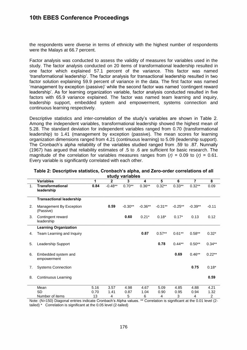
10th EBES Conference Proceedings
176
the respondents were diverse in terms of ethnicity with the highest number of respondents were the Malays at 66.7 percent. Factor analysis was conducted to assess the validity of measures for variables used in the study. The factor analysis conducted on 20 items of transformational leadership resulted in one factor which explained 57.1 percent of the variance. This factor was named ‘transformational leadership’. The factor analysis for transactional leadership resulted in two factor solution explaining 59.9 percent of variance in the data. The first factor was named ‘management by exception (passive)’ while the second factor was named ‘contingent reward leadership’. As for learning organization variable, factor analysis conducted resulted in five factors with 65.9 variance explained. The factor was named team learning and inquiry, leadership support, embedded system and empowerment, systems connection and continuous learning respectively. Descriptive statistics and inter-correlation of the study’s variables are shown in Table 2. Among the independent variables, transformational leadership showed the highest mean of 5.28. The standard deviation for independent variables ranged from 0.70 (transformational leadership) to 1.41 (management by exception (passive). The mean scores for learning organization dimensions ranged from 4.21 (continuous learning) to 5.09 (leadership support). The Cronbach’s alpha reliability of the variables studied ranged from .59 to .87. Nunnally (1967) has argued that reliability estimates of .5 to .6 are sufficient for basic research. The magnitude of the correlation for variables measures ranges from (r) = 0.09 to (r) = 0.61. Every variable is significantly correlated with each other.
Table 2: Descriptive statistics, Cronbach’s alpha, and Zero-order correlations of all study variables
Variables 1 2 3 4 5 6 7 8 1.
Transformational leadership
0.84 -0.48** 0.70** 0.36** 0.32** 0.33** 0.32** 0.09
Transactional leadership
2. Management By Exception (Passive)
0.59 -0.30** -0.36** -0.31** -0.25** -0.39** -0.11
3. Contingent reward leadership
0.60 0.21* 0.18* 0.17* 0.13 0.12
Learning Organization
4. Team Learning and Inquiry
0.87 0.57** 0.61** 0.58** 0.32*
5. Leadership Support 0.78 0.44** 0.50** 0.34**
6. Embedded system and empowerment
0.69 0.46** 0.22**
7. Systems Connection 0.75 0.18*
8. Continuous Learning 0.59
Mean 5.16 3.57 4.98 4.67 5.09 4.85 4.88 4.21 SD 0.70 1.41 0.87 1.04 0.90 0.95 0.94 1.32 Number of items 13 4 5 6 4 3 4 2
Note: (N=150) Diagonal entries indicate Cronbach’s Alpha values. ** Correlation is significant at the 0.01 level (2-tailed) * Correlation is significant at the 0.05 level (2-tailed)

10th EBES Conference Proceedings
177
To further investigate the relationships among the variables, a series of multiple regression analyses between independent variables (transformational leadership, management by exception (passive) and contingent reward leadership) and the dependent variables (team learning and inquiry, leadership support, embedded system and empowerment, systems connection and continuous learning) were conducted. As shown in Table 3, four regressions were found to be significant: team learning and inquiry, R² = 0.177; leadership support, R² = 0.13; embedded system and empowerment, R² = 0.12 and system connection, R² = 0.18. Continuous learning was found not significant towards any of the independent variable. The independent variables explained 17.7 percent of the variance in team learning and inquiry; 13.3 percent of the variance in leadership support; 12.7 percent of the variance in embedded system and empowerment, 18.7 percent of the variance in systems connection and .9 percent of the variance in continuous learning. Transformational leadership was found to be the predictor for team learning and inquiry, leadership support, embedded system and empowerment; and systems connection. However, transformational leadership seen to be a more important predictor to embedded system and empowerment than team learning and inquiry, leadership support and systems connection. Hypothesis 1 is thus partially supported. Management by exception (passive) and contingent reward leadership did not predict any of the learning organization dimensions thus giving no support to Hypothesis 2.
Table 3: Multiple regression for leadership styles and learning organization
Variables Team Learning and Inquiry Std B
Leadership Support Std B
Criterion Embedded system and empowerment Std B
Systems Connection Std B
Continuous Learning Std B
Predictor Transformational Leadership
0.29**
0.27*
0.36**
0.30**
-0.02
Transactional Leadership Contingent Reward Leadership MBEP
-0.07 -0.24**
-.07 -0.20*
-0.11 -0.12
-0.16 -0.30**
0.12 -0.09
R² 17.7 13.3 12.7 18.7 2.1 F 10.47** 7.49** 7.1** 11.23** 1.06
N= 150. *p<.05; **p<.01
6. DISCUSSION This study was designed to gain insight in the building of learning organizations from the perspective of leadership styles. It has been proposed that transforming into learning organizations is imperative to meet the present business environment and certain leadership styles impact the building of learning organizations. Specifically, this study examined the relationship between leadership styles of transformational leadership, management by exception (passive) and contingent reward leadership. Results showed that transformational leadership predicted team learning and inquiry, leadership support, embedded system and empowerment; and systems connection. Characterized by intellectual stimulation, individualized consideration, inspirational motivation and idealized influence, transformational leaders generate the development and change in an organization (Viitala, 2004). Hence, leadership styles that are characterized by inspirational and participative behavior, mutual trust, and respect for subordinates’ ideas and feelings tend to move towards as learning organizations compared to the leadership styles that are characterized by task oriented and autocratic behaviors. Intellectual stimulation encourages the organizational members to look at things from new perspectives and generate new ideas, hence encourage learning. Individualized consideration provides support to employees in the organization and therefore

10th EBES Conference Proceedings
178
help in the building of learning organization. By articulating vision of leaders through inspirational motivation, employees have clear and compelling view of what leaders expected in them to better improve the organization. This help to evolve into learning organizations (Johnson, 2002). Leaders also need to give emphasize on the moral and inferences of their decisions and sacrifice for the betterment of the organization as indicated in idealized influence to build a learning organization. The above findings support studies by Amitay et al. (2005), Aragon-Correa et al. (2007), Coad and Berry (1998), Politis (2002), Singh (2008) and Zagorsek et al. (2009) that transformational leadership is necessary to facilitate learning in the organization. As for transactional leadership, management by exception (passive) and contingent reward leadership do not predict any of the learning organization dimensions. Indeed management by exception (passive) indicated significant negative relationships on a few learning organization dimensions. This explains that leaders who fail to intervene until problems become serious hinder learning in an organization. Although we anticipated relationship between contingent reward leadership and learning organization dimensions the results showed otherwise and this surprised us. This can be explained by firstly, looking at the context of manufacturing organizations. Clarifying roles and task requirements are more inclined towards routine works and specialization hence does not encourage learning. Even though rewards are contingent on the fulfilment of the task, employees are not willing to learn new things as they are rewarded based on only the completion of the task. Secondly, another reason that could contribute to this is the responding organizations are undergoing change due to the pressures of the business environment therefore transformational leadership are more appropriate compared to transactional leadership which is more effective in a stabilize condition (Bass, 1985). The contributions of this study are of importance, firstly, due to the fact that this is an empirical work. As most writings on learning organization are conceptual in nature (Popper and Lipshitz, 2000; Zagorsek et al. 2009), therefore it is imperative to fill the gap of scarce empirical work on the topic especially in Malaysia. Secondly, this study empirically proves that leadership that are characterized by leaders that inspire the morale and motivation of their subordinates i.e., transformational leadership is crucial in building a learning organization. From a theoretical point of view, this study integrates two different fields of learning organization and leadership from an empirical perspective. The present study suggests some implications for human resource managers and the top management on the important role of leaders in promoting learning at all levels and provide opportunities for people in their organization to learn. This also suggests that in building a learning organization, more leadership training focusing on transformational leadership style should be conducted. The findings of this study raised several limitations that should be considered in pursuing future research. First, the sample of this study was from the manufacturing industry and it can only be generalized within that context only. Further expansion of the research across different industries and geographical regions would significantly contribute to the better understanding of the relationship between leadership styles and building a learning organization. Secondly, this study employed a cross-sectional study design, which focuses on issues at one point in time, over a longitudinal design. Since becoming a learning organization is not an overnight process and the interrelationships between the variables evolve over time, future research should consider the use of a longitudinal design to obtain such details. A longitudinal treatment of data might yield additional insights in the impact of transformational leadership and learning organization. Finally, this study is limited to the direct effect of leadership styles on learning organization. Future study should include

10th EBES Conference Proceedings
179
moderating or mediating variables such as organizational culture to get a better understanding of the relationship between leadership styles and building a learning organization. 7. CONCLUSION In conclusion, this study builds on previous research showing that leadership styles specifically transformational leadership is significantly and positively related to building a learning organization. Back to the question asked at the beginning: Do leadership styles matter in building a learning organization? The answer here is a qualified yes. Which type of leadership style has a stronger influence on building a learning organization? The answer is transformational leadership style. The more top management practice transformational leadership style, the more the organizations are moving towards to be learning organizations. REFERENCES Abu Daud, S., 2009. Leadership theories, research and practice: Framing future leadership thinking. Serdang: Universiti Putra Malaysia. Amitay, M., Popper, M., and Lipshitz, R., 2005. Leadership styles and organizational learning in community clinics. The Leadership Organization, 12(1), pp.57-70. Angela, M., Silva, K., and Leila, M., 2011. Leadership styles correlate of learning organization in a non-western culture. The Business Review, 17(2), pp.269-277 Aragon-Correa, J.A., Garcia-Morales, V.J., and Cordon-Pozo, E., 2007. Leadership and organizational learning's role on innovation and performance: lessons from Spain. Industrial Marketing Management, 36(3), pp.349-359. Atak, M. and Erturgut, R., 2010. An empirical analysis on the relation between learning organization and organizational commitment. Procedia Social and Behavioral Sciences, 2(2), pp.3472-3476. Bass, B. M., 1985. Leadership and performance beyond expectations. New York: Free Press. Bass, B.M., and Avolio, B.J., 1995. Multifactor leadership questionnaire. Palo Alto, CA: Mind Garden. Challis, D., Samson, D., and Lawson, A.B., 2005. Impact of technological, organizational and human resource investments on employee and manufacturing performance: Australian and New Zealand evidence. International Journal of Production Research, 43(1), pp.81-107. Coad, A.F., and Berry, A.J., 1998. Transformational leadership and learning orientation. Leadership & Organization Development Journal, 19(3), pp.164-172. Ellinger, A.D., Ellinger, A.E., Yang, B., and Howton, S.W., 2002. The relationship between the learning organization concept and firms’ financial performance: An empirical assessment. Human Resource Development Quarterly, 13(1), pp.5–21. Gunasekaran, A., 2004. Benchmarking in the internet era. Benchmarking: An International Journal, 11(5), pp.56-70.

10th EBES Conference Proceedings
180
Johnson J.R., 2002. Leading the learning organization: Portrait of four leaders. Leadership and Organization Development Journal, 23(5), pp.241-249. Marsick, V.J., and Watkins, K.E., 2003. Summing up: Demonstrating the value of an organization's learning culture. Advances in Developing Human Resources, 5(2), pp.129-131. Nafei, W.A., Khanfar, N.M and Kaifi, B.A., 2012. Leadership styles and organizational learning: an empirical study on Saudi Banks in Al-Taif Governorate Kingdom of Saudi Arabia. Journal of Management and Strategy, 3(1), pp.2-17. Norashikin, H., Noormala, A.I., Fauziah, N., Norzaidi, M.D., and Chong, S.C., 2009. The effect of human resource practices on building learning organisations: Evidence from Malaysian manufacturing firms. International Journal of Innovation and Learning, 6(3), pp.259-274. Nunnaly, J.C., 1967. Psychometric theory. New York: McGraw-Hill. Popper, M. and Lipshitz, R., 2000. Organizational learning mechanisms, culture, and feasibility. Management Learning, 31(2), pp.181-196. Rowden, R.W., 2000. The relationship between charismatic leadership behaviors and organizational commitment. The Leadership & Organization Development Journal, 21(1), pp.30-35. Sahaya, N., 2013. A learning organization as a mediator of leadership style and firms’ financial performance. International Journal of Business and Management, 7(14), pp.96-113. Senge, P.M., 1990. The fifth discipline: The art and practice of the learning organization. New York: Doubleday. Singh, K., 2008. Relationship between learning organization and transformational leadership: Banking organizations in India. International Journal of Business and Management Science, 1(1), pp.97-111. Vera, D. and Crossan, M., 2004, Strategic leadership and organizational learning. Academy of Management Review, 29(2), pp.222-240. Watkins, K. E. and Marsick, V. J., 1996. A framework for the learning organization. IN: Sage. Watkins, K.E. and Marsick, V.J., 1997. Dimensions of the learning organization. Warwick, RI: Partners for the Learning Organization. Yang, B., 2003. Identifying valid and reliable measures for dimensions of a learning culture. Advances in Developing Human Resources, 5(2), pp.152-162. Yeo, R., 2003. Linking organizational learning to organizational performance and success: Singapore case studies. Leadership and Organization Development Journal, 4(2), pp.70–83. Zagorsek, H. Dimovski, V., and Skerlavaj, M., 2009. Transactional and transformational leadership impacts on organizational learning. Journal of East European Management Studies, 14(2), pp.144-165.
10th EBES Conference Proceedings 23 - 25 May, 2013. NIPPON HOTEL, ISTANBUL, TURKEY ISBN: 978-605-64002-1-6. WEBSITE: www.ebesweb.org
181
AIR TRAFFIC DELAYS, SAFETY, AND REGULATOR’S
OBJECTIVES: A MONOPOLY CASE
CHUNAN WANG Toulouse School of Economics
University of Toulouse France
[email protected] Abstract: Aimed at reducing air traffic delays, this paper proposes a contract signed between the regulator and the monopoly airline to implement a delay reduction service. Different from previous literature, in this paper, the expected delays per flight are only a function of safety levels and the regulator's objective function is a weighted sum of the monopoly airline's profit, passenger surplus, and the regulator's profit. This paper first derives and compares the optimal contracts under complete and incomplete information. Then, this paper shows that the effects of the increases of safety levels on the optimal degrees of the delay reduction service depend on the safety elasticity of delay and the safety elasticity of cost. This paper also shows that the changes of the weights can create different incentives for the regulator to adjust the optimal degrees. Moreover, this paper proposes some relevant policy recommendations for the regulator. Keywords: Air Traffic Delays, Safety, Regulator’s Objectives, Contract, Policy Recommendations 1. INTRODUCTION The Single European Sky ATM1 Research (SESAR) project started by the Council of the European Union at 2006 aims at satisfying future capacity and safety needs at a European level. The Council plans to enable a 3-fold increase in capacity which also reduces air traffic delays, improve the safety performance by a factor of 10, and enable a 10% reduction in the effects flights have on the environment.2 Particularly, in the context of the SESAR project, airlines can reveal their preferences in the regulation, which means that the regulator can sell services to airlines to help them reduce delays3 and costs. The motivation of this paper is to study the optimal contracts signed between the regulator and the monopoly airline. Specifically, this paper tries to study the effects of the information structures (complete and incomplete information), safety levels, and the regulator's objectives on the optimal contracts. Moreover, according to the analysis, this paper tries to propose some relevant policy recommendations for the regulator.
I acknowledge Estelle Malavolti for her insightful comments and unfailing support. I also thank Daniel Garrett, Yong Sui, Gang Wang, Miaomiao Dong, Lei Liu, and the participants of 10th EBES Conference, Istanbul, Turkey, 2013 ECORE Summer School “Governance and Economic Behavior”, Leuven, Belgium, and China Meeting of the Econometric Society 2013, Beijing, China for helpful discussions. Needless to say, I am responsible for all remaining errors. 1 ATM is an abbreviation for Air Traffic Management.
2 The European Air Traffic Management Master Plan - Edition 1 (European Commission and EUROCONTROL,
2009). 3 In some studies, there is a difference between schedule delay and flight delay (Basso, 2008). Schedule delay is
the gap between passengers' actual and desired departure time while flight delay can be measured by the gap between flight actual and scheduled arrival time. Relative to flight delay, schedule delay is more subjective because it mainly depends on passengers' desire. Thus, this paper only focuses on flight delay, i.e., air traffic delays in this paper refer to flight delay.
10th EBES Conference Proceedings
182
In general, congestion and safety consideration are the two main factors resulting in air traffic delays. According to Cohen et al. (2009), if airlines neglect the costs they impose on the others, they always schedule more flights exceeding the capacity of airspace and airports. Then, congestion may probably happen. This is the congestion externality problem. Generally speaking, there is a trade-off between safety levels and delays, i.e., the higher the safety level the regulator maintains is, the more likely the delays happen. Some accidental factors, for example, bad weather and technical problems, are serious threats to air traffic safety. Thus, the regulator may create some delays to ensure safety. To solve the congestion externality problem, there are mainly two kinds of approaches, price-based approaches (Basso, 2008; Brueckner, 2002; Pels and Verhoef, 2004; Yang and Zhang, 2011; Zhang and Zhang, 2003; 2006; 2010) and quantity-based approaches (Basso and Zhang, 2010; Brueckner, 2009; Cohen et al. 2009; Czerny, 2010; Verhoef, 2010). According to Brueckner (2009), under price-based approaches, the airport declares a charge per flight and then airlines choose the number of flights they wish to schedule. Price-based approaches can be implemented by either a differentiated, airline-specific congestion toll or a uniform per-flight charge. Particularly, Brueckner (2002) studied the optimal congestion toll under different market structures. If the airport is used by a monopoly airline, congestion can be fully internalized and thus there is no need to charge congestion toll. However, if the airport is used by several airlines, congestion can just be partially internalized and thus a toll is needed for uninternalized congestion. According to Brueckner (2009), under quantity-based approaches, the airport declares a total desired number of flights and then achieves by allocating a corresponding number of slots. Quantity-based approaches can be implemented by either a slot-distribution regime where a fixed total number of slots are distributed for free and then airlines are permitted to trade as they want or a slot-auction regime where slots are completely allocated through an auction. This paper, however, will not focus on congestion. On the one hand, according to the goals of the SESAR project, capacity will greatly expand, which implies that congestion may no longer be a serious problem in the future European sky and airports. On the other hand, this paper studies a monopoly case. According to Brueckner (2002), congestion can be fully internalized by a monopoly airline and thus does not exist. Therefore, this paper will use a new delay function, which is proposed in Wang (2013). Specifically, instead of the total number of flights and airport capacities, we will only model safety levels into the delay function, which is also consistent with the observation that safety consideration is the other main source of delays except congestion. To reduce the delays caused mainly by safety consideration, we will introduce a delay reduction service which can be provided by the regulator. In the context of the SESAR project, a new generation air traffic management system will be used by the regulator in the future, which makes a better coordination for flights possible. Thus, technically, the regulator will have the ability to reduce delays through the new management system. From the economic aspect, the regulator can sell the delay reduction service through a contract, in which the degree of the delay reduction service4 the regulator provides to the airline and the transfer the airline pays to the regulator are formulated. This paper is in fact a further study of Wang (2013), where the regulator sells the delay reduction service to duopoly airlines through a second-price sealed-bid auction. Wang (2013) focused on the relationship between the airlines' equilibrium bids and their types, the effect of
4 For the degree of the delay reduction service, we can understand in the following way. Suppose the regulator
can provide n items of the delay reduction service. If the airline buys i items, , then the degree is
(100i/n)%. The more items the airline buys from the regulator, the larger the degree of the delay reduction service will be.

10th EBES Conference Proceedings
183
the increases of safety levels on the regulator's equilibrium revenue, and in equilibrium, the effects of the mechanism on airlines competition and passenger surplus. This paper, however, derives and compares the optimal contracts under complete and incomplete information and studies the effects of the increases of safety levels on the optimal degrees of the delay reduction service. In this paper, the regulator's objective function is a weighted sum of the monopoly airline's profit, passenger surplus, and the regulator's profit. Therefore, this paper also studies the effects of the changes of the weights on the optimal degrees of the delay reduction service. In particular, there is a significant difference between this paper and some regulation literature (Baron and Besanko, 1984; Baron and Myerson, 1982; Laffont and Tirole, 1986). In those studies, the regulator's objective function is a weighted sum of consumer and producer surplus. In this paper, however, as we have described, the regulator's objective function also includes its own profit. To briefly summarize, this paper contributes to the literature of air traffic delays on three aspects. First, this paper uses a new delay function and a new regulator's objective function. Second, this paper proposes a contract to implement a delay reduction service. Specifically, the optimal contracts are incentive feasible and passengers can enjoy benefits from them. Third, this paper proposes some relevant policy recommendations for the regulator. The remainder of the paper is organized as follows. Section 2 introduces the model. Section 3 derives and compares the optimal contracts under complete and incomplete information. Moreover, this section studies the effects of the increases of safety levels and the changes of the weights on the optimal degrees of the delay reduction service. Besides, this section also studies four examples to illustrate some results. Section 4 concludes the paper and summarizes the policy recommendations proposed in the paper. 2. THE MODEL In this paper, the regulator sells a delay reduction service to the monopoly airline through a contract. Suppose that the monopoly airline is risk neutral and its profit before signing this contract is
where A is a parameter with A>0, denotes the airline's value of time, S denotes the safety levels the regulator maintains, and D(S) denotes the expected delays per flight. From this equation, we can see that the monopoly airline's profit decreases with air traffic delays.
We define as the airline's type. may be unobservable to the regulator. However, it is
common knowledge that belongs to the set , where and .
If is the airline's private knowledge, we assume that the airline can be either the one with
type or with probabilities v and 1-v respectively. For the safety levels, we assume that a
safety level is set by the regulator ex ante and satisfies the minimum requirement. Moreover, we assume that the expected delays per flight D(S) strictly increase with safety levels S, i.e.,
, which captures the fact that the higher safety level the regulator maintains is, the more likely the delays happen.

10th EBES Conference Proceedings
184
Remark 1. Usually, the delay function is modeled as
. The US Federal Aviation
Administration (1969) first proposed this specification and Horonjeff and McKelvey (1983) made a further discussion. Many studies, for example, Basso (2008), Morrison (1987), Oum, et al. (2004), and Zhang and Zhang (1997), used this specification in their models. Moreover, Yang and Zhang (2011) used a delay function which was linear in Q. In this paper, however, just because of the reasons we have discussed in Section 1, we use a new delay function, which is proposed in Wang (2013). Specifically, the expected delays per flight are only a function of safety levels, i.e., D(S). The regulator signs a contract with the monopoly airline. The contracting variables are R and T, where R is the degree of the delay reduction service the regulator provides to the airline and T is the transfer the airline pays to the regulator. After obtaining the delay reduction service, the monopoly airline's profit becomes
where is the fraction of delay reduction the airline can enjoy if the degree of the delay reduction service it purchases is R.
We assume , , and . This assumption implies that the marginal value of the delay reduction service is positive but strictly decreasing with the degree and the airline cannot enjoy any benefit if the degree it purchases is zero. Remark 2. In general, an airline has private knowledge mainly on two aspects, the fraction of delay reduction and the value of time. Wang (2013) models according to the first aspect while this paper models according to the second one. Suppose that passenger surplus is
where B is a parameter with B>0 and denotes the passengers' value of time. From this equation, we can see that passenger surplus decreases with air traffic delays. After the airline signs the contract, passengers will also enjoy delay reduction but pay nothing. Thus, passenger surplus becomes
We assume that the regulator tries to use the transfer to cover the cost of providing the delay reduction service. If the transfer is not enough, the regulator will use the revenue from its other activities to fill the gap. Then, according to this assumption, we can write the regulator's profit, i.e.,
where C(S) is the regulator's marginal cost of providing the delay reduction service, given a safety level. We assume that the regulator's marginal cost C(S) strictly increases with safety levels S, i.e., . In fact, when providing the delay reduction service, the regulator has to

10th EBES Conference Proceedings
185
schedule more staff if it hopes to achieve a higher safety level, which will inevitably result in a higher cost. From the perspective of normative analysis, the regulator should act as a social planner, whose objective is to maximize social welfare. However, in reality, this may not be the case, i.e., sometimes the regulator may put some emphasis on its own interests. Therefore, in this paper, we assume that the regulator includes its own profit as a part of its objective function. Of course, under some condition, the objective function of the regulator can be the one of a social planner. Suppose that the regulator's objective function is a weighted sum of the monopoly airline's profit, passenger surplus, and the regulator's profit, i.e.,
where , , and are the weights of , PS, and respectively with and
.
In particular, if
, the regulator actually acts as a social planner.
Remark 3. The regulator's objective function in this paper is significantly different from the one in some regulation literature. In those studies, the regulator's objective function is a weighted sum of consumer and producer surplus, without the regulator's profit. There are two reasons for the difference. On the one hand, the regulator in this paper is “the producer”, i.e., the regulator pays some costs to “produce” the delay reduction service and thus it will consider the costs when making decisions. On the other hand, in reality, sometimes the regulator does not act as a social planner, i.e., the regulator may put some emphasis on its own profit. Moreover, we assume that the regulator values more its own profit than the monopoly airline's profit, i.e., . In fact, when , the regulator will optimally set the transfer as lower as possible, which contradicts to the assumption that the regulator tries to use the transfer to cover the cost. Remark 4. From the equations above, we can clearly see that the model does not involve the airline's decision about the optimal number of flights it will schedule. The reason to make this assumption is to simplify the airline's decision process and thus facilitate us to focus on the regulator's decisions. The timeline is shown in Figure 1.
Figure 1: Timeline
t=0 time
t=2 t=3 t=1
Monopoly airline’s type becomes
common or private knowledge
Regulator offers a contract
Monopoly airline accepts
or refuses the contract
The contract is executed

10th EBES Conference Proceedings
186
3. ANALYSIS OF THE OPTIMAL CONTRACTS 3.1. Optimal contracts We first assume that the optimal contracts can ensure . Only under this assumption, the delay reduction service is socially valuable. Under complete information, the monopoly airline's type is common knowledge. The
regulator's optimization program for the airline with type can be written as
subject to
In this optimization program, and denote the degree of the delay reduction service and
the transfer respectively the regulator designs for the airline with type . Besides, the constraint is the monopoly airline's participation constraint.
Define . Plugging into the optimization program, we
can obtain
subject to
Optimally, the regulator will set . Plugging it into the objective function and taking the
first order condition with respect to , we can obtain
(1)
where
is the first-best degree of the delay reduction service for the airline with type from the regulator's perspective. For the second order derivative, we have
, which implies that
maximizes the objective function. Then, the first-
best transfer for the airline with type is
(2)
In exactly the same way, we can obtain the first-best degree of the delay reduction service and the first-best transfer for the airline with type , i.e.,
(3)
(4)
Finally, Lemma 1 summarizes the optimal contracts under complete information.

10th EBES Conference Proceedings
187
Lemma 1. Under complete information, the optimal contracts are
if and If , where
,
, , and are given by (1) to (4).
According to (1) and (3), because of and , we can obtain. Moreover, we can
also obtain
. These imply that, under complete information, the airline with a higher
value of time will enjoy a higher degree of the delay reduction service and pay a higher transfer to the regulator. Then, we will derive the optimal menu of contracts under incomplete information. According to Laffont and Martimort (2002), we first give the definition of incentive compatible.
Definition 1. A menu of contracts is incentive compatible when is weakly preferred to by the airline with type and is weakly preferred to by the airline with type . Under incomplete information, the monopoly airline's type is its private knowledge. In this case, in order to have the airline self-selecting properly within the menu, the incentive
compatibility constraints for the airline with type and must be satisfied, i.e.,
(5)
(6)
Moreover, the participation constraints must also be satisfied, i.e.,
(7)
(8)
Then, according to Laffont and Martimort (2002), we give the definition of incentive feasible. Definition 2. A menu of contracts is incentive feasible if it satisfies both the incentive compatibility and the participation constraints (5) through (8). Under incomplete information, the regulator's optimization program can be written as
subject to (5) to (8)
Define and as the information rent of the airline with
type and respectively. Plugging and into the
optimization program, we can obtain

10th EBES Conference Proceedings
188
subject to
(9)
(10)
(11)
(12)
We can find that (9) and (12) bind, i.e., and . Plugging them into the
objective function and taking the first order condition with respect to and , we can obtain
(13)
(14)
where
and are the second-best degrees of the delay reduction service for the airline
with type and respectively from the regulator's perspective.
For the second order derivative, we have
. Moreover, by
assuming
,5 we also have
. These conditions imply that
and
maximize the objective function.
Besides, we also have to check the other two omitted constraints. Obviously, can be
satisfied. According to (13) and (14), the monotonicity constraint
is satisfied. Thus,
we can also validate .
Then, the second-best transfers for the airline with type and are, respectively,
(15)
(16)
Finally, Lemma 2 summarizes the optimal menu of contracts under incomplete information. Lemma 2. Under incomplete information, the optimal menu of contracts
is incentive feasible and given by (13) to (16). Besides, only the
airline with type gets a positive information rent given by .
5 This assumption excludes corner solution. Without this assumption, the regulator will find it optimal not to sign a
contract with the airline with type .

10th EBES Conference Proceedings
189
We have seen
. Moreover, we can also obtain
. These imply that, under
incomplete information, the airline with a higher value of time will enjoy a higher degree of the delay reduction service and pay a higher transfer to the regulator. 3.2. Analysis We first compare the optimal contracts under complete and incomplete information. The comparison for the optimal degrees of the delay reduction service is given in Proposition 1. Proposition 1. Under incomplete information, for the optimal degrees of the delay reduction service, there is no distortion for the airline with type with respect to the first-best, i.e.,
. However, for the airline with type , with respect to the first-best,
1. there is a downward distortion, i.e., , when ; 2. there is no distortion, i.e., , when .
Proof. According to Lemma 1 and 2, we have
, which implies
,
i.e., under incomplete information, for the airline with type , there is no distortion with
respect to the first-best. When , we have , which implies ,
i.e., under incomplete information, for the airline with type , there is a downward distortion
with respect to the first-best. When , we have , which implies
, i.e., under incomplete information, for the airline with type , there is no distortion
with respect to the first-best. In the relevant literature, due to the asymmetric information, there always exists downward distortion. In this paper, however, there also exists the case where there is no distortion. In the following part, we will see how the regulator makes decisions. Under incomplete information, the regulator's objective function can be written as
(17)
where EAE denotes the Expected Allocative Efficiency, EIR denotes the Expected Information Rent, and
In the regulator's objective function, the expected information rent does not depend on ,
which implies that, under incomplete information, the regulator has no incentive to distort .
Then, we have
. However, the expected information rent does depend on . Therefore, according to the
values of and , we will analyze the regulator's incentive about distorting .
When , reducing the expected information rent will increase the value of the objective function. Therefore, under incomplete information, optimally, the regulator will distort

10th EBES Conference Proceedings
190
downward to reduce the information rent left to the airline with type and thus the
expected information rent. Then, we have .
Under , maximizing the objective function (17) with respect to , we can obtain
From the equation above, for the regulator, we can find a trade-off between efficiency and rent extraction. The left-hand side is the efficiency gains of the regulator from the infinitesimal
increase of while the right-hand side is the rent increase of the airline with type from the
infinitesimal increase of . In fact, is the value which balances the trade-off.
When , there is no expected information rent in the regulator's objective function. Therefore, under incomplete information, optimally, the regulator will not distort . Then, we
have .
Under , unlike the relevant literature, for the regulator, the trade-off between efficiency and rent extraction does not exist, which is due to the fact that the monopoly airline's profit is included in the regulator's objective function. In fact, for the case where , the amounts of the information rents do not affect the value of the objective function. Therefore, if we only consider the value of the objective
function, optimally, the information rents can be and , where
, which implies that the transfers for the airline with type and will be lower than
and respectively. However, we have assumed that the regulator tries to use the transfer
to cover the cost. Under this assumption, the regulator will only leave the necessary
information rents for the airline, i.e., . Therefore, under incomplete information,
when , the optimal transfers will still be
and
.
Then, the comparison for the optimal transfers is given in Corollary 1.
Corollary 1. For the airline with type ,
. For the airline with type , , when ; , when . Proof. According to Lemma 1 and 2, we can easily see Corollary 1. Thus, the proof is omitted henceforth.
In Corollary 1, for the airline with type , the reason why the second-best transfer is lower
than the first-best one is that, under incomplete information, the airline with type can obtain the information rent. For the airline with type , the comparison depends on whether the
regulator distorts downward under incomplete information. When , the regulator
distorts downward , which implies that the second-best transfer is lower than the first-best
one. When , the regulator does not distort , which implies that the second-best
transfer is equal to the first-best one.

10th EBES Conference Proceedings
191
From Proposition 1 and Corollary 1, we can see that, under incomplete information, the
regulator can achieve the first-best contract except a lower transfer for the airline with type , as long as it values equally its own profit and the monopoly airline's profit. Undoubtedly, safety is one of the most important factors in the air transport industry and the regulator always has incentives to increase safety levels. Therefore, we should study the effects of the increases of safety levels on the optimal degrees of the delay reduction service, which may provide some policy recommendations for the regulator about setting safety levels. Before proceeding to Proposition 2, we first give two definitions, the safety elasticity of delay and the safety elasticity of cost. Definition 3. The safety elasticity of delay is defined as
According to this definition, we can see that the safety elasticity of delay measures the
percentage change in delay in response to a one percent change in safety level. Definition 4. The safety elasticity of cost is defined as
In a similar way, the safety elasticity of cost measures the percentage change in cost in
response to a one percent change in safety level. Then, Proposition 2 summarizes the effects of the increases of safety levels on the optimal degrees of the delay reduction service.
Proposition 2. The optimal degrees of the delay reduction service
, ,
, and increase (resp. decrease) with safety levels S when (resp. ) .
Proof. Taking the derivative of
in Lemma 1 with respect to S, we can obtain
Therefore,
increases with safety levels S when
Note
and
. Rearranging the inequality and multiplying both sides by
S, we can obtain

10th EBES Conference Proceedings
192
According to Definition 3 and 4, we can obtain
where
is the safety elasticity of delay and
is the safety elasticity
of cost.
Otherwise,
decreases with safety levels S.
Moreover, the proof of ,
, and follows exactly the same way and is omitted
henceforth.
The intuition behind Proposition 2 is straightforward. According to the assumptions
and , the increases of safety levels will lead to longer delays and higher costs. Longer delays will motivate the regulator to choose higher degrees of the delay reduction service while higher costs will bring an opposite motivation for the regulator. Therefore, when the safety elasticity of delay is larger than the safety elasticity of cost, which implies that the effect of the increases of safety levels on delays is larger than those on costs, the motivation related to delays will dominate the one related to costs and thus the regulator will increase the optimal degrees of the delay reduction service. Otherwise, the motivation related to costs will dominate the one related to delays and thus the regulator will decrease the optimal degrees of the delay reduction service. The result in Proposition 2 is helpful for the regulator about setting safety levels. From Proposition 2, we can see that, when , the optimal degrees of the delay reduction
service may be very small when safety level is too high, which implies that the new generation air traffic management system may be less efficiently used. Therefore, knowing this possible situation, to ensure the efficient use of the new management system, the regulator can avoid setting a too high safety level when .
Finally, we will study the effects of the changes of the weights on the optimal degrees of the delay reduction service, which may provide some policy recommendations for the regulator about setting the weights. The result is given in Proposition 3. Proposition 3. Considering the effects of the changes of the weights on the optimal degrees of the delay reduction service, 1. the change of cannot create a direct incentive but can create an indirect one for the regulator to change
, , and
;
2. the increase (resp. decrease) of can create an incentive for the regulator to increase (resp. decrease) ; 3. the increase (resp. decrease) of can create an incentive for the regulator to increase (resp. decrease)
, ,
, and ;
4. the increase (resp. decrease) of can create an incentive for the regulator to decrease (resp. increase)
, ,
, and .
Proof. For , under complete information, optimally, the regulator will set the transfers and exactly the same with the benefits the monopoly airline can enjoy from the delay reduction
service and respectively. Then, in the objective function, does not

10th EBES Conference Proceedings
193
link directly to and any more and thus the change of does not directly affect
, and
. Moreover, under incomplete information, in the objective function, only links directly
to the information rent of the airline with type , which is a function of , not . Therefore, the
change of also does not directly affect
. However, we should notice the constraint
, which implies that the change of will inevitably lead to the change of at least one of the other two weights and . Therefore, we can say that the increase of cannot create a direct incentive but can create an indirect one for the regulator to change
, , and
. Furthermore, as we have mentioned, under incomplete information, links directly to the
information rent of the airline with type , which is a function of . Obviously, we can find that
the increase (resp. decrease) of can help reduce (resp. raise) the expected information
rent, which will thus incentivize the regulator to increase (resp. decrease) .
For analyzing the effects of the changes of and , let us take
as an example. Under
complete information, the following equation determines
, i.e.,
(18)
From the regulator's perspective, the left-hand side is the marginal utility while the right-hand side is the marginal cost. Normalizing the marginal cost to C(S), we can obtain
The increase (resp. decrease) of can help make the marginal utility larger (resp. smaller) than the marginal cost. Thus, to keep them equal, the regulator has incentive to increase
(resp. decrease)
. However, the increase (resp. decrease) of can help make the marginal utility smaller (resp. larger) than the marginal cost. Thus, to keep them equal, the
regulator has incentive to decrease (resp. increase)
.
Besides, the analysis of the effects of the changes of and on ,
, and follows
the same way as the example.6 Here, we should be careful that the changes of , , and can only affect the regulator's incentive to change the optimal degrees of the delay reduction service, but cannot determine the final adjustments. Whether the regulator eventually adjusts R as we expect depends on
the total effects of the changes of , , and . Let us take the increase of and the
change of
as an example. According to Proposition 5, the increase of can create an
incentive for the regulator to increase
. However, because the regulator may also change
, whether
will finally increase is uncertain. When the ratio
becomes higher,
will
increase. Otherwise,
will decrease.
6 Comparing with (18), the equation which determines contains a marginal information rent. In fact, due to the
existence of the marginal information rent, the increase (resp. decrease) of can create an additional incentive
for the regulator to decrease (resp. increase) .

10th EBES Conference Proceedings
194
From Proposition 3 and the following analysis, we can obtain Corollary 2. Corollary 2. Given other parameters unchanged, 1. when the ratio
becomes higher (resp. lower),
, ,
will be larger (resp. smaller);
2. when the ratios
and
become higher (resp. lower) at the same time or one of them
becomes higher (resp. lower) and the other is unchanged, will be larger (resp. smaller); otherwise, besides
and
, the change of also depends on , v, and .
Proof. Just as (18), we can also write the equations which determine ,
, and .
Dividing these equations by on both sides, we can easily see the Corollary 2. Thus, the proof is omitted henceforth. The intuition behind Corollary 2 is as follows. Because the airline and passengers can enjoy benefits from the delay reduction service, they have a positive need for a higher degree of
the service. Moreover, the increases of
and
imply that, relative to its own profit, the
regulator puts more emphasis on the airline's profit and passenger surplus. Therefore, to better satisfy the need of the airline and passengers, the regulator will optimally respond by
increasing the degrees of the delay reduction service. However, when
and
change in
the opposite directions, the regulator's decision about how to change becomes
complicated and also depends on some other parameters besides the ratios. The results in Proposition 3 and Corollary 2 are helpful for the regulator about setting the weights. From Proposition 3 and Corollary 2, we can see that, when the regulator reduces the weights of the monopoly airline's profit and passenger surplus a lot, the optimal degrees of the delay reduction service may be very small, which implies that the new generation air traffic management system may be less efficiently used. Therefore, knowing this possible situation, to ensure the efficient use of the new management system, the regulator can avoid reducing the weights of the monopoly airline's profit and passenger surplus a lot. 3.3. Examples In this part, we will study four examples to illustrate the results in Proposition 1 and Corollary 2.
Example 1.
.
In this example, the regulator acts as a social planner and cares about the social welfare.
The optimum in this example, denoted by
,
,
, and
, are
,
;
,
.

10th EBES Conference Proceedings
195
Example 2.
.
In this example, the regulator cares only about the sum of the monopoly airline's profit and its own profit but nothing about passenger surplus. In reality, this example does not likely exist because the regulator always places great emphasis on consumers. Here, we only discuss it theoretically.
The optimum in this example, denoted by
,
,
, and
, are
,
;
,
.
Example 3.
.
In this example, the regulator cares only about the sum of passenger surplus and its own profit but nothing about the monopoly airline's profit. This example is essentially an extreme one for the fact that sometimes the regulator cares more about consumers than firms.
The optimum in this example, denoted by
,
,
, and
, are
,
;
,
.
Example 4. . In this example, the regulator cares only about its own profit but nothing about the monopoly airline's profit and passenger surplus. This example is similar to the models in some principal-agent literature, where the principal cares only about its own profit.
The optimum in this example, denoted by
,
,
, and
, are
,
;
,
.
Comparing the optimal degrees of the delay reduction service, under complete information, we obtain

10th EBES Conference Proceedings
196
Under incomplete information, for the airline with type , with respect to the first-best, we can obtain
,
,
,
.
Moreover, we have
For the airline with type , with respect to the first-best, we can obtain
,
,
,
.
Moreover, when
, we have
when
, we have
To make the comparison easier to see, we show these optimal degrees of the delay reduction service in Figure 2 and 3.
Figure 2: Optimal degrees (when
)
R
R
123 123( , )FB FB
R R
123 123( , )SB SB
R R
23 23( , )FB FB
R R
13 13( , )FB FB
R R
13 13( , )SB SB
R R
3 3( , )FB FB
R R
23 23( , )SB SB
R R
3 3( , )SB SB
R R

10th EBES Conference Proceedings
197
Figure 3: Optimal degrees (when
)
Then, we analyze the examples as follows.
First, the examples illustrate the result in Proposition 1. For the airline with type , in every example, the second-best degree of the delay reduction service is equal to the first-best one. However, for the airline with type , in Example 3 and 4, the second-best one is smaller than
the first-best one; in Example 1 and 2, the second-best one is equal to the first-best one. In fact, the comparison above is consistent with the result in Proposition 1, i.e., under incomplete information, with respect to the first-best, there is no distortion for the airline with
type , while for the airline with type , there is a downward distortion when and no
distortion when .
Second, the examples also illustrate the result in Corollary 2.
in Example 1 are the
highest ratios and we can see that
,
,
, and
are the largest degrees.
in Example 4 are the lowest ratios and we can see that
,
,
, and
are
the smallest degrees.
in Example 3 is higher than
in Example 2 and we can see
that
,
, and
are larger than
,
, and
respectively. Moreover, there are
and
in Example 2 and
and
in Example 3 and we can see that,
besides
and
, the comparison between
and also depends on the passengers'
value of time and the degree of downward distortion
. When the degree of downward
distortion is relatively low, i.e.,
, we can see that
is larger than . However,
when the degree of downward distortion is relatively high, i.e.,
, we can see that
is smaller than
.
R
R
123 123( , )FB FB
R R
123 123( , )SB SB
R R
23 23( , )FB FB
R R 13 13( , )FB FB
R R
13 13( , )SB SB
R R
3 3( , )FB FB
R R
23 23( , )SB SB
R R
3 3( , )SB SB
R R
10th EBES Conference Proceedings
198
4. CONCLUSIONS AND POLICY RECOMMENDATIONS Under the background of the SESAR project, this paper proposed a contract signed between the regulator and the monopoly airline to implement a delay reduction service. Different from previous literature, this paper used a new delay function, which was proposed in Wang (2013). Specifically, instead of the total number of flights and airport capacities, this paper only modeled safety levels into the delay function. Moreover, the regulator's objective function in this paper was a weighted sum of the monopoly airline's profit, passenger surplus, and the regulator's profit. To reduce the delays caused mainly by safety consideration, we introduced a delay reduction service and proposed a contract in which the degree of the delay reduction service and the transfer are formulated. After deriving the optimal contracts, we compared the optimal degrees of the delay reduction service under complete and incomplete information. We found that, under incomplete information, for the airline with a high value of time, there was no distortion with respect to the first-best. However, for the airline with a low value of time, there was a downward distortion or no distortion with respect to the first-best, which depended on the weights of the regulator's profit and the monopoly airline's profit. Moreover, we also compared the optimal transfers under complete and incomplete information. Then, we showed that the optimal degrees of the delay reduction service increased with safety levels when the safety elasticity of delay was larger than the safety elasticity of cost and decreased with safety levels otherwise. Furthermore, we showed that the changes of the weights could create different incentives for the regulator to adjust the optimal degrees of the delay reduction service. Besides, we studied how the ratios of the weights determined the changes of the optimal degrees. Generally speaking, relative to its own profit, if the regulator puts more emphasis on the airline's profit and passenger surplus, the optimal degrees will increase. In the last part, we studied four examples to illustrate some of the results above. This paper is rather policy-oriented. Throughout the paper, there are four main policy recommendations as the following. First, the regulator should be aware of the fact that, for the future European air transport industry, safety levels will become the most significant factor determining air traffic delays. Second, the optimal contracts are incentive feasible and passengers can enjoy benefits from them. Therefore, it is worthwhile for the regulator to implement these optimal contracts. Third, under incomplete information, by valuing equally its own profit and the monopoly airline's profit, the regulator can achieve the first-best contract except a lower transfer for the airline with a high value of time. Fourth, the regulator should avoid setting a too high safety level when the safety elasticity of delay is smaller than the safety elasticity of cost. Moreover, the regulator should also avoid reducing the weights of the monopoly airline's profit and passenger surplus a lot. Otherwise, the new generation air traffic management system may be less efficiently used. REFERENCES Baron, D.P. and Besanko, D., 1984. Regulation, asymmetric information, and auditing. The RAND Journal of Economics, 15(4), pp.447-470. Baron, D.P. and Myerson, R.B., 1982. Regulating a monopolist with unknown costs. Econometrica, 50(4), pp.911-930. Basso, L.J., 2008. Airport deregulation: Effects on pricing and capacity. International Journal of Industrial Organization, 26(4), pp.1015-1031.
10th EBES Conference Proceedings
199
Basso, L.J. and Zhang, A., 2010. Pricing vs. slot policies when airport profits matter. Transportation Research Part B: Methodological, 44(3), pp.381-391. Brueckner, J.K., 2002. Airport congestion when carriers have market power. The American Economic Review, 92(5), pp.1357-1375. Brueckner, J.K., 2009. Price vs. quantity-based approaches to airport congestion management. Journal of Public Economics, 93(5-6), pp.681-690. Cohen, J.P., Coughlin, C.C., and Ott, L.S., 2009. Auctions as a vehicle to reduce airport delays and achieve value capture. Federal Reserve Bank of St. Louis Review, 91(6), pp.569-587. European Commission and EUROCONTROL, 2009. The European air traffic management master plan - Edition 1. Czerny, A.I., 2010. Airport congestion management under uncertainty. Transportation Research Part B: Methodological, 44(3), pp.371-380. Horonjeff, R. and McKelvey, F.X, 1983. Planning and design of airports. Third edition, USA: McGraw-Hill. Laffont, J.-J., and Martimort, D., 2002. The theory of incentives: The principal-agent model. New Jersey: Princeton University Press. Laffont, J.-J., and Tirole, J., 1986. Using cost observation to regulate firms. Journal of Political Economy, 94(3), pp.614-641. Morrison, S.A., 1987. The equity and efficiency of runway pricing. Journal of Public Economics, 34(1), pp.45-60. Oum, T.H., Zhang, A., and Zhang, Y., 2004. Alternative forms of economic regulation and their efficiency implications for airports. Journal of Transport Economics and Policy, 38(2), pp.217-246. Pels. E., and Verhoef, E.T., 2004. The economics of airport congestion pricing. Journal of Urban Economics, 55(2), pp.257-277. US Federal Aviation Administration, 1969. Airport capacity handbook. Washington DC: US Government Printing Office. Verhoef, E.T., 2010. Congestion pricing, slot sales and slot trading in aviation. Transportation Research Part B: Methodological, 44(3), pp.320-329. Wang, C., 2013. Air traffic delays, safety, and airline strategies: A duopoly case. Toulouse School of Economics working paper. Yang, H. and Zhang, A., 2011. Price-cap regulation of congested airports. Journal of Regulatory Economics, 39(3), pp.293-312. Zhang, A. and Zhang, Y., 1997. Concession revenue and optimal airport pricing. Transportation Research Part E: Logistics and Transportation Review, 33(4), pp.287-296.

10th EBES Conference Proceedings
200
Zhang, A. and Zhang, Y., 2003. Airport charges and capacity expansion: Effects of concessions and privatization. Journal of Urban Economics, 53(1), pp. 54-75. Zhang, A. and Zhang, Y., 2006. Airport capacity and congestion when carriers have market power. Journal of Urban Economics, 60(2), pp.229-247. Zhang, A. and Zhang, Y., 2010. Airport capacity and congestion pricing with both aeronautical and commercial operations. Transportation Research Part B: Methodological, 44(3), pp.404-413.
10th EBES Conference Proceedings 23 - 25 May, 2013. NIPPON HOTEL, ISTANBUL, TURKEY ISBN: 978-605-64002-1-6. WEBSITE: www.ebesweb.org
201
CORPORATE GOVERNANCE DISCLOSURE: A CASE OF BANKS IN MALAYSIA
NASUHA NORDIN
Institute of West Asian Studies University Kebangsaan Malaysia
Malaysia [email protected]
MOHAMAD ABDUL HAMID
Institute of West Asian Studies University Kebangsaan Malaysia
Malaysia [email protected]
Abstract: Knowledgeable investors in present days, has somehow triggered demand for more information and disclosure of companies to make decision. Corporate governance disclosure in many countries are still a voluntary disclosure in general, with possibility a minimal mandatory disclosures (Samaha, et al., 2012). Most studies conducted on corporate governance disclosure are mainly done on the more developed countries, as it is perceived to have a complete if not the latest framework for such disclosure need (Samaha, et al., 2012). Till to date, Malaysia has introduced three Code of Corporate Governance first being in 2000, followed by 2007 and the latest in 2012. The objectives of this paper are to discuss on three matters, (1) evolvement of corporate governance code of practice in Malaysia, (2) determinants of corporate governance disclosure of banks in Malaysia, and (3) similarities and differences of corporate governance disclosure of Islamic and Conventional Banks. Keywords: Corporate Governance Disclosure, Conventional Banks, Islamic Banks, Malaysian Code of Corporate Governance 1. INTRODUCTION Corporate governance disclosure in many countries is still a voluntary disclosure in general, with possibility of minimal mandatory disclosures (Hassan, 2009, Samaha, et al., 2012). Corporate governance as defined by Bank Negara Malaysia (‘BNM’) as “the process and structure used to direct and manage the business and affairs of the institution towards enhancing business prosperity and corporate accountability with the ultimate objective of realizing long term shareholder value, whilst taking into account the interests of other stakeholders” (Bank Negara Malaysia, 2011; Hassan, 2009). Most studies conducted on corporate governance disclosure or risk management disclosure are mainly done on the more developed countries, as it is perceived to have a complete if not the latest framework for such disclosure need (Hassan, 2009; Samaha, et al., 2012). With knowledgeable stakeholders and investors, there is indication of demand for further disclosure in the annual reports other than the mandatory financial and non-financial disclosure. In corporate governance subject areas, most studies done are on the conformity and compliance of corporate governance in various industries and countries, legal framework as mechanism of corporate governance, history and landscape of corporate governance
10th EBES Conference Proceedings
202
practice. These studies are usually associated with determinants such as firm characteristics, ownership structure and corporate governance characteristics. It is noted that research on disclosure of corporate governance and risk management has been minimal over the years (Abu-Tapanjeh, 2009; Bhatti and Bhatti, 2009; Hassan, 2009; Samaha, et al., 2012). Knowledgeable investors in present day have somehow triggered demand for more information and disclosure of companies to make decision. Bauwhede and Willekens (2008) and Samaha et al. (2012) study the extent of corporate governance disclosure in association with firm characteristics, ownership structure, and corporate governance characteristics for Europe companies and Egypt respectively. Bauwhede and Willeken (2008) finds further that, other firm characteristics are also associated to corporate governance disclosure; short and long term accruals, legal framework (e.g.: countries in common law discloses more than other legal framework), US cross listing, change in stock price, change in long term debt, and change in total assets. Samaha et al. (2012) finds that different ownership structure affects corporate governance disclosure (CGD) differently; number of shareholders is positively related to CGD, while block holder ownership is negatively related, and director ownership has no significant impact on CGD. Samaha et al. (2012) also highlighted that proportion of non-executive directors are positively related to CGD. The research will enrich the literature on disclosure of corporate governance and risk management. The research also will highlight the comparison between the two dependent variables cross country and region of Malaysia, as most research done are on one country, hence this study will give insight on comparison between the two countries. Findings of CGD extent, can be use as a benchmark for regulators, and professional bodies to further enhance disclosure effectiveness and enforcement among the IFIs (Samaha, et al., 2012). Minimal literature on Islamic corporate governance (Abu-Tapanjeh, 2009; Bhatti and Bhatti, 2009; Hassan, 2009) and Islamic Financial Institutions (‘IFIs’) risk management (Samaha, et al., 2012). Malaysian banks both conventional and Islamic, disclosures and reporting is governed by the Company’s Act 1965, Bank Negara Malaysia (Central Bank of Malaysia), and International Financial Reporting Standards, Banking and Financial Institutions Act, 1989, Islamic Banking Act 1983 respectively. 2. PRIOR STUDIES This section will discuss on prior studies done on corporate governance and corporate risk disclosure from both perspective of conventional and Islamic perspective from financial and non financial firms. 2.1. Prior studies by country Various studies have been carried out in prior years pertaining to corporate governance (CG) and risk management (RM). Among the common studies are corporate governance implementations and how it affects of being affected by several determinants, credit risk management and the relevant determinants and affects on firm value, disclosure studies either general, accounting, corporate governance, credit risk management, risk factors, and corporate risk disclosure which either mandatory or voluntary disclosures. These studies have been conducted in various countries or regions, among the studies conducted are Bahrain (Al-Ajmi, 2009; Hassan, 2009), Singapore (Eng and Mak, 2003), Belgium (Hassan, 2009; Willekens and Knechel, 2004), Hong Kong (Gul and Leung, 2004; Hassan, 2009; Ho
10th EBES Conference Proceedings
203
and Shun Wong, 2001), Australia (Henry, 2009), US (Beasley, et al., 2005), Malaysia (Abdul Wahab, et al., 2007; Hassan, 2009; Yatim, 2009), Asian countries (Kaneko, 2007), West Asian countries and Malaysia (Farook, et al., 2011), US, UK, Germany and Japan (Shleifer and Vishny, 1997), Egypt (Samaha, et al., 2012), and Canada (Maingot and Zeghal, 2008). Most of the study done are would somehow relate to certain firm characteristics as determinant of corporate governance and risk management implementation or disclosure. Corporate governance and risk management studies have been done all over the world. Several studies have been done on Malaysia with regards to CG and RM, however, minimal study have been done on Bahrain. Farook et al. (2011) study on West Asian countries and Malaysia is more about corporate social responsibilities (CSR) disclosure as part of CG mechanism and CSR disclosure determinants. Hence this study intends to explore more on CG disclosure as a whole rather than just CSR, of Malaysian banks practices. 2.2. Financial vs. non-financial firms Mehran et al. (2011) highlight that corporate governance and risk management structures for financial and non financial firms are different in many ways, this is mainly due to the fact nature of business. Other worth noting differences between financial and non financial firms characteristics identified in Mehran et al. (2011) study are, debt composition, stakeholders dispersion, opaqueness of daily activities, insolvency impact of countries’ or global financial market, potential free rider monitoring, risk attitudes of shareholders, leverage position within the company as product for financial firms and source of finance for non financial firms, ability to alter risk composition, and executive pay. Due to opaqueness of financial firms, a well structured corporate governance and risk management is more critical than non financial firms. Hence, this study tries to explore the several financial firms’ characteristics including opaqueness of financial firms’ activities, executive pay, debt composition, risk composition and other relevant factors and how it’s being communicated via disclosure of Corporate Governance (CG). Financial and non financial firms are different in many ways, same goes for conventional banks and Islamic banks corporate governance structure. As far as Bhatti and Bhatti (2009) and Abu Tapanjeh (2009) are concern, Islamic and conventional corporate governance (CCG) are different in some ways with several similarities. The studies compared the Islamic perspective on corporate governance in comparison with Organisation for Economic Cooperation and Development (OECD) corporate governance. OECD corporate governance has been embraced or is being transplanted in some developing countries throughout the world (Kaneko, 2007).
2.3. Islamic corporate governance vs. conventional corporate governance OECD corporate governance principles includes; ensuring basis of an effective CG framework, CG framework should protect and facilitate exercise of shareholders rights, CG framework should ensure that equitable treatment of all shareholders including minority and foreign shareholders, CG framework should also ensure that strategic guidance of the company, the effective monitoring of the management by the board and accountability to the company and the shareholders, role of stakeholders is to recognized by creating wealth jobs, and sustainability of financially sound enterprise, and disclosure and transparency (Bhatti and Bhatti, 2009). Abu Tapenjeh (2009) has categorized OECD principles into four main categories which are; (1) mechanism of business ethics, (2) mechanism for decision making, (3) adequate disclosure and transparency, and finally (4) mechanism of book keeping and final accounts.
10th EBES Conference Proceedings
204
Islamic corporate governance (ICG) principles includes principles are base on Shariah law, ensuring all rights of all stakeholders are adhered to, equitable distribution of wealth to stakeholders, use of Shura concept, and disclosure and transparency (Abu-Tapanjeh, 2009; Bhatti and Bhatti, 2009). Abu Tapanjeh (2009) has highlighted several differences and has divided it into categories which based from OECD CG principles (ensuring basis for an effective CG framework, rights of shareholders and key ownership functions, equitable treatment of shareholders, role of stakeholders in CG, disclosure and transparency, and responsibilities of the board). Firstly, the study highlighted major difference between ICG accountability are not only limited to shareholders, or stakeholders, but to ultimate accountability is towards God. Secondly, OECD CG is shareholder centered, while ICG is stakeholders centered. Thirdly, OECD CG vision on equitable treatment are limited to minority and foreign shareholders only, while ICG scope is wider, it covers all relevant stakeholders, not only on profit distribution to shareholders but also Zakat and Sadaqa for the needy and poor. Finally, disclosure and transparency guidelines base on OECD CG guidance covers on matters regarding corporation, financial situation, and performance, ownership and governance only. On the other hand ICG covers in greater deal, including Shariah compliance disclosure, socio economic objectives related to firm’s control and accountability to all its stakeholders, justified and truthfulness transparency, and wider accountability with written as well as oral disclosure (Abu-Tapanjeh, 2009). The main differences between conventional corporate governance (CCG) and Islamic corporate governance (ICG) are legal structure of governance (Shariah Law or conventional law), accountability (God, shareholders, stakeholders), distribution of wealth (zakat, dividend) (Abu-Tapanjeh, 2009; Bhatti and Bhatti, 2009). Hence this study will try to find whether there are any significant differences in CGD between conventional and Islamic banks, as this area of study is still lacking of empirical research. Due to more information needed for disclosure of Islamic Corporate Governance, empirical research on disclosure for corporate governance using ICG is a more beneficial empirical research contribution to literature on corporate governance. 2.4. Firm characteristics Prior studies have identified various firm characteristics either as determinant of CGD, CG compliance, corporate risk disclosure, risk management tools used, or as control variables of such empirical research. The most common firm attributes being included as variable of CG or RM research are firm size (Bauwhede and Willekens, 2008; Beasley, et al., 2005; Eng and Mak, 2003; Gul and Leung, 2004; Hassan, 2009; Ho and Shun Wong, 2001; Linsley and Shrives, 2006), leverage (Amran, et al., 2009; Bauwhede and Willekens, 2008; Eng and Mak, 2003; Gul and Leung, 2004; Hassan, 2009; Ho and Shun Wong, 2001), and industry type (Beasley, et al., 2005; Eng and Mak, 2003; Hassan, 2009; Ho and Shun Wong, 2001). Other attributes are, growth opportunities, analyst following, stock price performance, profitability, stock volatility, audit fee, audited by Big5/ Big4 audit firm, overseas listing, equity market liquidity, firm issued new share capital following year, short term accrual, non common law, change in stock price, political connection, Bumiputra directors, reserves, product diversification, geographical diversification, market to book equity ratio, listing status, equity financing, liquidity, and high quality of accounting standard. Hence for the purpose of this study, the common firm character such as firm size and leverage will be included, as being part of control variables. IBs in Malaysia are expected to be of different size and leverage composition due to different financial clientele. Having Big4 (formerly Big5) as auditor has a mixed findings being not significant association with voluntary disclosure (Eng and Mak,
10th EBES Conference Proceedings
205
2003) and positive association to enterprise risk management implementation association (Beasley, et al., 2005) needs further empirical evidence on association with CGD. Firm growth, stock price performance and profitability also had mixed findings, Eng and Mak (2003) finds no significant association between the variables with voluntary disclosure, while Gul and Leong (2004) find that there is a positive association with voluntary disclosure, hence need for more empirical evidence on the mixed findings. 2.5. Ownership structure There are various types of ownership structure such as directors’ ownership, block holders’ ownership, managerial ownership, government ownership, concentrated ownership, institutional ownership, external ownership, dispersed ownership and so on. Among the commonly debated type of ownership in relation to corporate governance implementation, risk management implementation and disclosure are directors’ ownership, and block holders’ ownership. Eng and Mak (2003) found no significant association between block holder ownership and level of voluntary disclosure, while Samaha et al. (2012) found a negative association between block holder ownership and CGD. Block holders might have the power to influence the decision made within the firm, however, prior study showed that block holder either does not encourage or are not bothered with disclosure matters, either overall voluntary disclosure or specific disclosure such as corporate governance disclosure (CGD). Hence, this type of ownership structure could be the negative determinant for level of disclosure for CGD, which might explain the fact that block holder owners that might not need additional disclosure, as they are more closely related to board members, as well the management, hence couldn’t be bothered to the extent of disclosure. Another ownership structure that is worth mentioning is directors’ ownership. Samaha et al. (2012) in contrast to negative association of block holder ownership with CGD, finds that directors’ ownership has no significant association with CGD. On the other hand, Gul and Leong (2004) find a negative association between voluntary disclosure and directors’ ownership. Referring to block holder ownership, directors’ ownership variable, has a similar effect on the level of disclosure. Hence, directors’ ownership should also be considered as determinant that negatively affect the level of CGD. Eng and Mak (2003) also discussed about other types of ownerships that are associated with voluntary disclosure. Managerial ownership is negatively, while government ownership is positively, associated with voluntary disclosure. Bauwhede and Willekens (2008) find that there is a negative association between concentrated ownership and CGD. Abdul Wahab et al. (2007) find a positive association between institutional ownership and corporate governance compliance. It can be concluded that, ownership that is controlled by certain influential holders (block holder, directors, concentrated, institutional, and government) has somehow significant effect either positively or negatively on level of disclosure. Hence, structure of ownership will be among the significant determinant to level of CGD. 2.6. Corporate governance OECD defined corporate governance as ‘Procedures and processes according to which an organization is directed and controlled. The corporate governance structure specifies the distribution of rights and responsibilities among the different participants in the organization – such as the board, managers, shareholders and other stakeholders – and lays down the rules and procedures for decision-making’(European Central Bank, 2004). Corporate
10th EBES Conference Proceedings
206
governance issues, discourse and empirical research started as early as 1970s (Bhimani, 2009). However, the research in this area has become more popular since the introduction of Cadbury Report, combined Report, Hampel Report, Turnbull Report, Higgs Report and Smith Report. These reports show the evolution of corporate governance reports over the years. Studies on corporate governance include relationships studies, landscape studies, agency theories relation, legal framework relation and many more. The most common research done is the empirical studies on relationships of corporate governance specific attributes and other variables. Prior study on corporate governance mainly focused on several areas, which includes specific CG attributes, CG compliance, CG disclosure, CG codes implementations as well as emerging importance of Islamic Corporate Governance compared to conventional CG codes. Henry (2009) study was an empirical research on CG compliance for a sample of listed companies in Australia. The study highlighted that greater conformity of CG codes and best practices in Australia, tends to lower the agency cost in short run as well as in the long run. Another way that the study can be conducted in order to further verify the validity of the empirical evidence is by looking at the compliance from the disclosure perspective. If the information on the compliance is evidence in either annual report, proxy circular or other publicly available information such as firms’ website, then the Henry (2009) findings of association will have better findings validity. 2.7. Corporate governance attributes Other researches on corporate governance are more focused on specific attribute of corporate governance (Ammann, et al., 2011); audit committee; (Al-Ajmi, 2009; Ho and Shun Wong, 2001), board composition (Beasley, et al., 2005; Eng and Mak, 2003), CEO duality (Gul and Leung, 2004; Yatim, 2009), proportion of experienced non executive directors (Gul and Leung, 2004; Ho and Shun Wong, 2001; Yatim, 2009), board meeting (Beasley, et al., 2005), appointment of dominant CEO (Ho and Shun Wong, 2001), proportion of family members (Ho and Shun Wong, 2001), CEO compensation (Hermalin and Weisbach, 2011), and board expertise and board diligence (Yatim, 2009). The most commonly discussed CG attributes is existence of audit committee and proportion of non-executive directors. Eng and Mak (2003), Gul and Leong (2004), and Ho and Shun Wong (2001) finds a positive association with voluntary disclosure, however, Samaha, et al. (2012) finds no significant association with corporate governance disclosure. This might be due to the fact that country understudy was of different legal regime, and different period of introduction of corporate governance code of practice. It is important variable to determine disclosure level of firms might it be corporate governance disclosure, corporate risk disclosure or other type of voluntary and mandatory disclosure. It also indicates that audit committee plays an important role in decision making for disclosure purpose. Proportion of non executive directors is also a commonly discussed CG variable among researchers (Beasley, et al., 2005; Eng and Mak, 2003; Gul and Leung, 2004; Ho and Shun Wong, 2001; Samaha, et al., 2012). Eng and Mak (2003), Gul and Leong (2004), and Ho and Shun Wong (2001) tried to find association of with voluntary disclosure. Eng and Mak (2003) and Gul and Leong (2004) found negative association with voluntary disclosure, however, Ho and Shun Wong (2001) found no association. However, this study believes that outside or non executive directors would want to show that they are performing well by indicating that they are doing well by having higher disclosure level for corporate governance and risk management, which is consistent with Samaha et al. (2012) findings of positive association of proportion of non executive directors with CG disclosure.
10th EBES Conference Proceedings
207
CEO duality is found to be negatively associated with voluntary disclosure and corporate governance disclosure by Gul and Leong (2004) and Samaha et al. (2012) respectively, however, Yatim (2009) finds that CEO duality has a positive association with risk management committee existence. The study showed that the separation of role of as CEO and Chairman of Board of Directors would result in a higher disclosure compared to firms that have duality role of CEO. It may be concluded that CEO dualities may affect the level of disclosure for CGD, negatively but at the same time may encourage formation of risk management committee. Hence, for the purpose of this study, CEO duality may be one of the determinants of CGD. Other corporate governance attributes that have been associated with voluntary disclosure, corporate governance compliance, and corporate governance disclosure (CGD) includes proportion of family members sitting on the board, appointment of dominant CEO, Bumiputra directors, and board size. Ho and Shun Wong (2001) find voluntary disclosure is negatively associated with proportion of family members sitting on board but did not find any significant association with appointment of dominant CEO. On the other hand Abdul Wahab et al. (2007) study finds positive association of CG compliance with Bumiputra directors. Samaha et al. (2012) finds a positive association between CGD and board composition in terms of size, and proportion of non-executive directors. It can be concluded that various corporate governance specific attributes are among the significant determinants of level of disclosure for CGD. 2.8. Corporate risk management attributes Yatim (2009) study finds that there are several determinants of existence of risk management committees in Malaysian firms. The study showed empirical findings that among the determinants of existence risk management committee covered from corporate governance attributes, risk management attributes, firms’ attributes, to ownership structure. Formation of risk management committee is positively determined by separation of CEO duality as CEO and as Chairman of Board of Directors, board expertise and diligence, firm size, firm listing status, complexity of the firms’ activities, and firm being in financial sector. Hence, it is expected in this study that overall view of attributes and determinants might influence the extent of disclosure for CG. Linsley and Shrives (2006), Amran et al. (2009), and Hassan (2009) all performed empirical research on risk disclosure in UK, Malaysia, and UAE respectively. Linsley and Shrives (2006), Amran et al. (2009), and Hassan (2009) all agreed that firm size and leverage are positively associated with level of risk disclosure, except that Linsley and Shrives (2006) did not highlight whether leverage is associated or not to risk disclosure. However, Linsley and Shrives (2006) highlighted that firms’ level of risk and environmental risk is positively associated with risk disclosure level. In addition, Amran et al. (2009) finds that leverage, product diversification, and geographical diversification are also positively associated to risk level of disclosure, and Hassan (2009) finds risk disclosure has positive association with industry type, but negatively associated with capital reserve from profit made for the financial period. 2.9. Summary Firm size and firm leverage are the most common variables used in association with CGD or voluntary disclosure. All of which is found to be positively associated with respective disclosure (Amran, et al., 2009; Bauwhede and Willekens, 2008; Eng and Mak, 2003;
10th EBES Conference Proceedings
208
Hassan, 2009; Linsley and Shrives, 2006). Other similar variables used by CGD and voluntary disclosure empirical research includes board size, outside directors, directors ownership, and block holder ownership (Eng and Mak, 2003; Gul and Leung, 2004; Ho and Shun Wong, 2001; Samaha, et al., 2012). CEO duality is found to be negatively associated to voluntary disclosure and CGD (Gul and Leung, 2004; Samaha, et al., 2012) , however, audit committee, director ownership and block holder ownership has mixed finding. Audit committees is found to be positively associated with voluntary disclosure (Gul and Leung, 2004; Ho and Shun Wong, 2001), however, no significant association found with CGD (Samaha, et al., 2012). Directors ownership were found not associated with CGD and voluntary disclosure by Samaha et al. (2012) and Eng and Mak (2003) respectively, however, Gul and Leung (2004) found a negative association with voluntary disclosure. Block holder ownership are negatively associated with CGD (Samaha, et al., 2012) and no significant association with voluntary disclosure (Eng and Mak, 2003). Hence this study will examine some of the common variables used in determining level of CGD. 3. MALAYSIA 3.1. Code of corporate governance time line Malaysia has introduced corporate governance in 2000 and since revised its code twice in 2007 and 2012 respectively. Each new Malaysia Code of Corporate Governance (MCCG) will supersede the prior ones. KLSE incorporates MCCG principles, and best practices in the corporate governance guidance of listed companies in Malaysia it be Main Market or the ACE Market (formerly known as MESDAQ Market). MCCG provides the basic Principles, Recommendations and Commentaries, KLSE will enhance the basic guidance in order to encourage shareholders involvement and their rights protections. Bank Negara Malaysia (BNM) constructed “Guidelines on Corporate Governance for Licensed Institutions” on MCCG as well as BIS Guidelines on “Enhancing Corporate Governance for Banking Organisation”. This guideline is applicable to all institutions which are licensed under BAFIA, namely commercial banks, investment banks and money makers. “Guidelines on Corporate Governance for Licensed Islamic (GP1-i)” is applicable to Islamic bank licensed under the Islamic Banking Act 1983 (excluding International Islamic Bank), Islamic bank holding company and any other institution specified by Bank Negara Malaysia. Guidelines on corporate governance for companies or firms incorporated in Malaysia is basically based on MCCG, however KLSE and BNM has respective specific requirements that companies or firms need to adhere to. Ultimately, all the guidelines or codes have a similar objective, which is to protect the interest of the respective stakeholders. 3.2. Malaysian Code Of Corporate Governance (MCCG) During the initial stage of forming MCCG, the council members have taken a few best practices as guidance to form the respective principles and best practice. These include the Hampel Report, Greenbury, Cadbury Code of Best Practice, Kuala Lumpur Stock Exchange listing requirements, and Toronto Stock Exchanges best practices. In 2000, the MCCG was divided into four parts mainly (1) Principles, (2) Best Practices in Corporate Governance, (3) Exhortations to Other Participants, and (4) Explanatory Notes and “Mere Best Practices”. Then in 2007 revision it was reduced to three parts by excluding Part 4 Explanatory Notes and “Mere Best Practices”. Most of the explanatory notes were not

10th EBES Conference Proceedings
209
totally abolished but rather combined with the other three parts remaining. Finally in 2012, this layout was totally revamped and combined and presented in manner of Principles and Recommendations. MCCG 2012 consists of eight principles and accompanied by 26 recommendations. All three MCCG are of the emphasis on role of board of directors to oversee the performance of the respective companies. Similar principles or best practice or recommendations made are existence of board of directors, size of board of directors, composition of executive and non-executive directors including independent directors, appointment of board of directors, re-election of board of directors, directors remuneration policies and procedures, roles of directors, rights of directors to have access to information and professional advises, disclosure of procedures and policies undertaken by the board, and existence of nomination committee, remuneration committee and audit committee. All three MCCG also clearly states that a narrative statement is required to disclose the in the narrative statement of how companies have applied the principles of MCCG and clearly states any non compliance of such principles in the annual report. In MCCG 2007, there are two amendments made to the existing principles and best practice of corporate governance. Firstly, audit committee should only consist of non executive directors. Secondly, instead of audit committee meeting with external auditors at least once a year, the meeting should be held at least twice a year. Furthermore, MCCG 2007 has added a few more principles and best practices. Firstly, nominating committee should ensure that yearly assessment and evaluations of directors are well documented. Secondly, it is required that all members of the audit committee to be financially literate and at least one member should be a member of an accounting association or body. Thirdly, improves communication between senior managers and chairman of audit committee of the company. Fourthly, the board should establish internal audit function and appoint head of internal audit function who reports to the audit committee. It can be seen that MCCG 2007 other than strengthening the existing principles, it has put into light the importance of audit committee and establishment of internal audit team to ensure better performance of the respective companies. MCCG 2012, we can see that the whole code of corporate governance layout has been revamped by combining it into eight principles and 26 recommendations as mentioned earlier. There are some new elements introduced in MCCG 2012. Among the new items are, introduction of board charter, annual assessment of directors independence, tenure of independent director should not exceed nine years, separation of role of CEO and chairman, board should set out expectations on time commitment for its members and protocols for accepting new directorships, use of information technology for effective dissemination of information, board to encourage poll voting, and board should have more gender mix (women). 3.3. MCCG disclosure requirement The MCCG states that there are several disclosure requirements in the annual report that public listed companies in Malaysia need to adhere to. Firstly, narrative statements of how they apply the relevant principles on their particular circumstances. Secondly, compliance of the voluntary best practices set out in the Code, and justifying for any non-compliances. These disclosures need not be a separated in the annual report, it is allowed to be combined to a certain degree. However, in Part 4 of the Code, “mere best practices” disclosure is not a mandatory disclosure as compared to the priors.
10th EBES Conference Proceedings
210
Since MCCG 2000, these have been the disclosure in the annual report requirements that are still intact. Firstly, details on the remuneration of each directors, disclose whether one third of the board are independent directors, whether Chairman and CEO role are combined, annual review of mix skills and experience and other qualities and core competencies that non-executive directors (NED) brings to the board, number of board meetings held in a year, details of attendance of each individual director in respect of meeting held, membership of remuneration committee, and audit committees’ details of activities, number of meetings held during the year and details of attendances of each individual director in respect of meetings. In MCCG 2007 additional disclosure requirement is disclosing details of relevant training attended by each director. MCCG 2012 recommended even further disclosure in the annual report which includes, nomination and election process of board members, gender diversity policies and targets and the measure taken to meet those targets, board remuneration policies and procedures, whether independent directors independence assessment has been conducted, and main features of the company’s risk management framework and internal control system. Companies are also encouraged to disclose in their corporate website the followings; summary of code of conduct, periodical review and publish the board charter on the corporate website, and dedicated section on corporate governance. 3.4. Kuala Lumpur Stock Exchange (KLSE) KLSE has set out a list of listing requirements for all listed companies in Malaysia, this includes corporate governance requirements. The requirements outlined are similar to MCCG requirements, however, there are further detail requirements that MCCG did not mention, as MCCG is just a general guideline of principles and recommendations on corporate governance for companies. In the listing requirements, the followings are the matters that listed companies need to adhere to. The listing requirements sets out several areas of compliance, (1) directorship, (2) audit committee, (3) auditors, (4) internal auditors, and finally (5) disclosure of corporate governance requirements. The similarities that KLSE and MCCG have are as follows, the need of balanced composition of directors between executives and non-executives directors, rights of directors to access to timely information, advise and support from company’s secretary and advice from professional advise at the expense of the respective company, directors training requirement, existence of audit committee consisting of non-executive directors, chairman of audit committee must be an independent director, roles of audit committee, rights of audit committee, procedures and policies of audit committee, appointment of external auditors, and finally disclosure of corporate governance practices in the annual report. On the other hand, KLSE has outlined additional description on the corporate governance practices that MCCG did not highlight in the principles, recommendations or any explanatory notes. Among the requirements further explained in detail are compositions of board of directors, the criteria that individual director needs to fulfill, composition of audit committee, detailed content of audit committee report, quorum of audit committee meeting, and detailed criteria of external auditor appointed. KLSE also has highlighted the importance of directors training, the practice note and guidance note has specifically required that all new directors must attend Mandatory Accreditation Program (MAP) within four months of appointment.
10th EBES Conference Proceedings
211
KLSE listing requirements has put a lot of emphasis on the competencies of directors, both independent and non-independent directors, in order to discharge their duties accordingly to safeguard stakeholders’ interest. 3.5. KLSE disclosure requirements Disclosure of corporate governance according to KLSE listing requirements, are similar to MCCG disclosure principles and recommendations. Listed companies are required to disclose in the annual report the narrative statement of its corporate governance practices, how the principles and recommendations have been applied and reasons for recommendations not followed and the alternative to it. Other additional statements that KLSE has required listed companies to include in the annual reports are statement explaining the board of directors’ responsibilities for preparing the annual audited financial statements, and statement about the state of internal control of listed issuer as a group (KLSE, 2012). KLSE has outlined the compulsory disclosure requirements in form of a checklist. This checklist is constantly revised from time to time in order to fit the current demand for information for stakeholders and public in general. The checklist consists of 30 items that listed companies in the main market need to adhere to; includes (1) Information, (2) Statement Accompanying Notice of AGM, (3) Resolution of Special Business, (4) Corporate information, (5) Directors Information, (6) CEO information, (7) Managing Director, (8) Audit Committee Report, (9) Chairman’s Statement, (10) Corporate Governance Disclosure, (11) Directors Remuneration, (12) Board Meetings, (13) Utilization of Proceeds, (14) Share Buy-backs, (15) Options of Convertible Securities, (16) Depository Receipt Programme, (17) Sanctions and/or Penalties, (18) Non-audit fees, (19) Variations in results, (20) Profit Guarantee, (21) Material Contracts, (22) Analysis of Shareholdings, (23) Revaluation Policies, (24) List of Properties, (25) ESOS, (26) Continuing Education Programme, (27) Corporate Social Responsibilities, (28) Recurrent Related Party Transaction, (29) Accounts, and (30) Internal Audit. 11 of the 30 subjects in the checklist are corporate governance related subjects, which are (5) Directors Information, (6) CEO information, (7) Managing Director, (8) Audit Committee Report, (10) Corporate Governance Disclosure, (11) Directors Remuneration, (12) Board Meetings, (26) Continuing Education Programme, (27) Corporate Social Responsibilities, and (30) Internal Audit. 3.6. BNM guidelines on corporate governance Bank Negara Malaysia (BNM) has outlined the guidance for corporate governance for licensed institutions, licensed Islamic institutions and other financial institutions. For the purpose of this study, only guidelines for licensed institutions and licensed Islamic banks will be discussed in detail. BNM guideline for licensed institutions sets out 14 main principles supported by explanatory notes following. The principles are (1) headed by effective board, (2) board composition, (3) clear division of responsibilities, (4) formal and transparent process for the appointment of directors and CEO, (5) directors commitment, (6) board meeting, (7) assessment of directors and CEO, (8) Remuneration package for directors and CEO, (9) policies and procedures to handle conflict of interest, (10) separation of shareholder and management, (11) robust auditing requirements, (12) communications with shareholders/ stakeholders, (13)
10th EBES Conference Proceedings
212
conducting corporate governance in a transparent manner, and (14) board collective responsible on veracity of disclosures and management of risk. BNM guidelines for licensed Islamic banks have the same principles except for the additional general principle of activities must be in compliance with Shariah requirements. Other specific difference on guidelines of licensed institutions and licensed Islamic institutions are (1) policies, procedures, infrastructure, and Islamic banks’ operations, products and activities are in compliance with Shariah requirements, (2) specific requirement to have effective and comprehensive policies, procedures and infrastructure to protect the interest of depositors and investment account holders, (3) board comprehensive understanding on Islamic banks’ business, the nature of risk undertaken by the Islamic bank and its strategic direction, (4) board sufficient knowledge and understanding of the nature of Mudharabah and Musharakah financing or investments and the risk associated with these types of transactions, (5) internal audit function should complements Shariah committee in ensuring Shariah compliance in all aspect, (6) internal audit together with Shariah committee determining scope of Shariah committee and produce internal Shariah compliant report, and (7) internal auditors should acquire necessary training to enhance their Shariah compliance review skills. BNM guidelines on corporate governance and KLSE corporate governance listing requirements mostly have the same if not similar principles and best practices. Among the similarities includes, (1) board composition, (2) directors training, directors mix of skills and experience requirements, (3) rights, roles and responsibilities of directors, (4) written approval of appointment of directors from BNM and KLSE, (5) existence of various board committees (Audit committee, Nomination committee, and Remuneration Committee), and (6) general disclosure requirements on comply or explain as stipulated in the MCCG. Among the difference between KLSE corporate governance listing requirements and BNM guidelines on corporate governance includes; (1) directors training, KLSE specifically required newly appointed directors to attend MAP training, while BNM only mention briefly about directors’ training, and (2) requirement of comprehensive understanding for financial market and the risk involved in each transactions undertaken by the licensed institutions or licensed Islamic institutions. Much like KLSE, BNM has extended several principals of MCCG to accommodate the specific requirement of the financial market industry. Corporate governance guidelines outlined by BNM are merely just an extension of MCCG code and BIS corporate governance best practice. Among the details that is not mentioned by MCCG are (1) directors comprehension and sufficient knowledge on financial markets and transactions, and risk face by the respective licensed institutions or licensed Islamic institutions, (2) specific qualification of independent directors in relation to holding of a substantial interest in the licensed institutions or licensed Islamic institutions, (3) sharing of independent directors within the group, (4) specific legal requirement and approval needed for appointment of directors, and (5) Shariah Committee roles, responsibility and rights. 3.7. Disclosure BNM guidelines for licensed institutions BNM guidelines on corporate governance for licensed institutions and licensed Islamic institution consists of 34 and 39 disclosures items within 10 and 11 headings respectively. The disclosure requirements set out by BNM are (1) board as a whole, (2) nominating committee, (3) remuneration committee, (4) risk management committee, (5) audit committee, (6) risk management, (7) internal audit and control activities, (8) related party transaction, (9) management report, (10) non-adherence to guidelines, and (11) Shariah committee. The disclosure requirements are mostly about the roles, responsibilities,

10th EBES Conference Proceedings
213
functions and rights of directors and respective board committees, background of directors, policies and procedures of risk management, related party transaction and conflict of interest, discussion of management reports, and statements on compliance or in some cases non-adherence to the guidelines explanations and alternative measures taken to comply. 3.8. Summary Malaysia has from time to time improves the code of corporate governance principles and recommendations to help the board to perform better to meet corporate objectives alongside the management. The codes also shows that emphasize on disclosure is greater each time code of corporate governance is revised that will in turn encourage participation of shareholders as they have more information on operations of their companies. MCCG 2012 also pointed the need to disclose the risk management and internal control system which is an important element for decision making of shareholders, investors and other stakeholders. KLSE listing requirements and BNM guidelines on corporate governance are based on the MCCG, however, KLSE and BNM has set out several additional and more detailed requirements of corporate governance attributes and disclosures. This could be due to MCCG is just a guide while KLSE and BNM are a binding requirements that needs to be adhere to by listed companies, and licensed institution and licensed Islamic institutions. Hence we can see that there are several corporate governance principles and disclosure requirements that overlap one another. MCCG has outlined the basic principles and recommendations of corporate governance practices, and base on that, KLSE has taken initiatives to another step by detailing practices that listed companies need to adhere to in order to encourage shareholders involvement and their rights protections. BNM guidelines on corporate governance, specifically caters for financial markets industry in Malaysia. This research will need to incorporate MCCG, KLSE Listing Requirements and accompanying Practice Note and Guidance Note of Corporate Governance, and BNM Guidelines on Corporate Governance in order to identify the mandatory and voluntary disclosures made by conventional and Islamic banks. This study will refer to the latest form of guidelines and code of practice for point of reference; i.e.; MCCG 2012, KLSE Listing Requirements 2012, and BNM Guidelines on Corporate Governance 2011. The reason being, that latest code, guidelines and requirements are assumed to be the most complete best practice for Malaysian companies. 4. CONCLUSION Malaysia has from time to time improves the code of corporate governance principles and recommendations to help the board to perform better to meet corporate objectives alongside the management. The codes also shows that emphasize on disclosure is greater each time code of corporate governance is revised that will in turn encourage participation of shareholders as they have more information on operations of their companies. MCCG 2012 also pointed the need to disclose the risk management and internal control system which is an important element for decision making of shareholders, investors and other stakeholders. KLSE listing requirements and BNM guidelines on corporate governance are based on the MCCG, however, KLSE and BNM has set out several additional and more detailed requirements of corporate governance attributes and disclosures. This could be due to MCCG is just a guide while KLSE and BNM are a binding requirements that needs to be adhere to by listed companies, and licensed institution and licensed Islamic institutions.

10th EBES Conference Proceedings
214
Hence we can see that there are several corporate governance principles and disclosure requirements that overlap one another. MCCG has outlined the basic principles and recommendations of corporate governance practices, and base on that, KLSE has taken initiatives to another step by detailing practices that listed companies need to adhere to in order to encourage shareholders involvement and their rights protections. BNM guidelines on corporate governance, specifically caters for financial markets industry in Malaysia. Studies on disclosure of corporate governance of Malaysia banking sector is still in the infancy stage, despite the fact that there has been much discourse on the relations studies between corporate governance attributes and performance. More research need to be performed on corporate governance disclosure extent and various variables including corporate governance attributes. REFERENCES Abdul Wahab, E., How, J.C.Y. and Verhoeven, P., 2007. The impact of Malaysian Code of Corporate Governance: Compliance, institutional investors and stock performance. Journal of Contemporary Accounting & Economics, 3(2), pp.106-129. Abu-Tapanjeh, A.M., 2009. Corporate governance from the Islamic perspective: A comparative analysis with OECD principles. Critical Perspectives on Accounting, 20(5), pp.556-567. Al-Ajmi, J., 2009. Audit firm, corporate governance, and audit quality: Evidence from Bahrain. Advances in Accounting, 25(1), pp.64-74. Ammann, M., Oesch, D. and Schmid, M.M., 2011. Corporate governance and firm value: International evidence. Journal of Empirical Finance, 18(1), pp.36-55. Amran, A., Bin, A.M.R. and Hassan, B.C.H.M., 2009. Risk reporting: An exploratory study on risk management disclosure in Malaysian annual reports. Managerial Auditing Journal, 24(1), pp.39-57. Bank Negara Malaysia, 2011. Guidelines on corporate governance for licensed Islamic banks (gp1-i). Kuala Lumpur Bauwhede, H.V. and Willekens, M., 2008. Disclosure on corporate governance in the European Union. Corporate Governance: An International Review, 16(2), pp.101-115. Beasley, M.S., Clune, R. and Hermanson, D.R., 2005. Enterprise risk management: an empirical analysis of factors associated with the extent of implementation. Journal of Accounting and Public Policy, 24(6), pp.521-531. Bhatti, M. and Bhatti, I., 2009. Development in legal issues of corporate governance in Islamic finance. Journal of Economic & Administrative Sciences, 25(1), pp.67-91. Bhimani, A., 2009. Risk management, corporate governance and management accounting: emerging interdependencies. Management Accounting Research, 20(1), pp.2-5.
10th EBES Conference Proceedings
215
Eng, L.L. and Mak, Y.T., 2003. Corporate governance and voluntary disclosure. Journal of Accounting and Public Policy, 22(4), pp.325-345. European Central Bank, 2004. Annual report 2004. In: ECB (ed). Frankfurt. Farook, S.Z., Lanis, R. and Hassan, K.M., 2011. Determinants of corporate social responsibility disclosure: The case of Islamic banks. Journal of Islamic Accounting and Business Research, 2(2), pp.114-141. Gul, F.A. and Leung, S., 2004. Board leadership, outside directors’ expertise and voluntary corporate disclosures. Journal of Accounting and Public Policy, 23(5), pp.351-379. Hassan, M.K., 2009. UAE corporations-specific characteristics and level of risk disclosure. Managerial Auditing Journal, 24(7), pp.668-687. Henry, D., 2009. Agency costs, ownership structure and corporate governance compliance: a private contracting perspective. Pacific-Basin Finance Journal, 18(1), pp.24-46. Hermalin, B.E. and Weisbach, M.S., 2011. Information disclosure and corporate governance. Fisher College of Business: The Ohio State University. Ho, S.S.M. and Shun Wong, K., 2001. A study of the relationship between corporate governance structures and the extent of voluntary disclosure. Journal of International Accounting, Auditing and Taxation, 10(2), pp.139-156. Kaneko, Y., 2007. Theories and realities of Asian corporate governance: From transplantation to the Asian best practices. Proceeding - Social and Behavioral Sciences, 2(5), pp.6883-6895. KLSE, 2012. Main market listing requirements. Kuala Lumpur: Bursa Malaysia Securities Berhad. [online] Available at: <http://www.bursamalaysia.com/market/regulation/rules/listing-requirements/main-market/listing-requirements> [Accessed 21 October 2012] KLSE, 2012. Ace market listing requirements. Kuala Lumpur: Bursa Malaysia Securities Berhad. [online] Available at: < http://www.bursamalaysia.com/market/regulation/rules/listing-requirements/ace-market/listing-requirements/> [Accessed 21 October 2012] Linsley, P.M. and Shrives, P.J., 2006. Risk reporting: A study of risk disclosures in the annual reports of UK companies. British Accounting Review, 38(4), pp.387-404. Maingot, M. and Zeghal, D., 2008. An analysis of corporate governance information disclosure by Canadian banks. Corporate Ownership & Control, 5(2), pp.225-236. Mehran, H., Morrison, A. and Shapiro, J., 2011. Corporate governance and banks: What have we learned from the financial crisis? Federal Reserve Bank of New York Staff Reports (Staff Report no. 502). [online] Available at: <http://ssrn.com/abstract=1880009> or <http://dx.doi.org/10.2139/ssrn.1880009> [Accessed 21 November 2012] Samaha, K., Dahawy, K., Hussainey, K. and Stapleton, P., 2012. The extent of corporate governance disclosure and its determinants in a developing market: The case of Egypt. Advances in Accounting, 28(1), pp.168-178.

10th EBES Conference Proceedings
216
Shleifer, A. and Vishny, R.W., 1997. A survey of corporate governance. The Journal of Finance, 52(2), pp.737-783. Willekens, M. and Knechel, W.R., 2004. The role of risk management and governance in determining audit demand. University of Florida: Department of Applied Economics, pp.1-35. Yatim, P., 2009. Board structures and the establishment of a risk management committee by Malaysian listed firms. Journal of Management and Governance, 14(1), pp.17-36.
10th EBES Conference Proceedings 23 - 25 May, 2013. NIPPON HOTEL, ISTANBUL, TURKEY ISBN: 978-605-64002-1-6. WEBSITE: www.ebesweb.org
217
IMPORTANCE AND ROLE OF SOCIAL MATURITY IN THE CONCEPT OF HOLISTIC MANAGERIAL COMPETENCE
JAN PORVAZNIK
Department of Management University of Economics in Bratislava
Slovak Republic [email protected]
JURAJ MISUN
Department of Management University of Economics in Bratislava
Slovak Republic [email protected]
Abstract: Social maturity becomes currently more and more important, because egoism,
pursuit of wealth, shoddy and unscrupulous people are today dominating. Thanks to these qualities of humans, organizations and society as a whole, we can determine the nature of people and their personality. It also works in the professional life, because character qualities of management subjects constitute the top of social maturity. Social maturity is besides manager knowledge and application skills the key pillar of the holistic managerial competence. It is a conscious or unconscious observance of basic human principles of behavior, enabling them to maintain the holistic of personality. A man becomes social mature through qualities that he receives either through genetic heritability or the environment in which he raises and educates. Through questionnaire method, we examined opinions of management subjects on each of the three pillars of the holistic managerial competence. 300 respondents from Slovakia and Czech Republic belonged either to a group of managers, full-time or part-time students. The aim of this paper is to outline the views of management subjects on the social maturity in the concept of holistic management and to make recommendations for improvement of the operation of the holistic model of managerial competence. Keywords: Social Maturity, Social Intelligence, Holistic Managerial Competence,
Sustainable Development 1. INTRODUCTION The importance of social maturity as an integral part of the holistic managerial competence increases. Among the myriad reasons for this increase are human selfishness, corruption, chasing to become rich and the like. There are certainly many people with developed social maturity, those who would be capable of solving current global problems. Such people, who can think beyond themselves, beyond their immediate family or very close friends. For these people, it is important that as well their colleagues in the team, the whole organization in which they work, or the region or country where they live, benefit. The problem is that these people are rare in the society. Even worse is the fact that the highest positions in politics often get people who do not meet the above requirements. If ordinary people see top politicians craving for money and power, negative examples create in them, which they often follow. How great do you think is the motivation of simple workers to pay taxes (mainly value added tax), when they see that their money is lost in numerous black holes? And it was right here, where we found opportunities

10th EBES Conference Proceedings
218
to research who is really a holistically capable individual. 2. CONCEPT OF HOLISTIC MANAGERIAL COMPETENCE Social sciences oriented on finance, economics, performance, management, marketing as well as on leadership offer number of definitions of competitiveness and recommendations on how to be a skilled leader. In principle the teachings improve only the development of manipulative skills. Kosturiak (2013, p.9) notes: “After some time, I realized that leadership is not about charisma and outer speech, but the inner nature of man, his integrity and actions”. In his article he also notes that many leaders of today are characterized by a desire for power, pride and a sense of infallibility that is the worst of human traits and that cause crisis and destruction. (Kosturiak, 2013) Politicians and managers of multinational corporations talk about growth of gross domestic product, growth of consumption, and production and sales growth. Only few people, among them also us, scientific and academic staff, talk about growth of happiness, humanity, happy family life, free time for human development, growth of welfare in our country and society in which we live. The literature counts several definitions of competence. We have found near one hundred of them. The approaches to their classification, or structuring, are different, often without reasoning and they are often eclectic. Many experts point out the fact that a broad extent of unsorted competencies is the reason for their refusal and lack of use in practice. In the current social environment accompanied by a number of crisis problems in the politics, in business, in social sphere and in education, in medical care, in culture, in mass media area, even those who have caused them call, for expert solutions. We call for experts to take over positions in management and other highly responsible positions. We consider an expert to be a person who knows everything necessary about a specific area. The knowledge results from their professional position, and it is expected that the person also possesses required skills and can apply the knowledge in case studies, solving of problems and tasks of everyday life. We question less whether an expert that disposes of necessary knowledge and is able to apply it in practice will also use it for his/her own benefit, by any means, at any price, even at risk of trespassing the legal, moral, ethical norms and principles or when applying it, he/she will think of other people's wellbeing, cooperation, social impulses from the surrounding environment, where he is a member of a team, unit, organization, region, country, continent, where he/she lives and works. In literature and in practice of hiring of managers and others to positions there are many approaches for creation of manager competence. Various authors define a great number of such competencies (psychologists use the term competencies, while they do not speak of responsibilities, authorities, but of required features), reasoning that in the time of computers there is no problem with assessment (Christopher, 2007; Albrecht, 2006; Goleman, 2006). The same approaches for their classification, or structuring, are different, often without reasoning and they are often eclectic. Many experts point out the fact that a broad extent of unsorted competencies is the reason for their refusal and limited use in practice. In the current social environment which is accompanied by a number of crisis problems in the politics, in business, in social sphere and in education, in medical care, in culture, in mass media, we all cry, even those who have caused it and are causing it, for expert solutions. We cry for experts to perform as managers and other positions.

10th EBES Conference Proceedings
219
An expert is considered such person who knows everything necessary resulting from tasks of their work and not only that they know it, but they even have required skills and ability to be able to implement the knowledge in solving the problems and tasks brought about by everyday life. Less we ask ourselves, if the expert with necessary knowledge who can implement them, uses those only for the benefit of himself, at any cost, even at cost of breaking the legal, ethical or moral standards and rules, or, if he considers people he works with and the social human stimulation of the surroundings, where these activities are applied, where the person is a member of a team, unit, organization, region, country, continent, planet, where he works and lives. Since the nineties we started to work on detailing of competencies of managers which are inherent to every single person. Here we note that for simplification we will implement the term holistic intelligence HQ, which consists of cognitive prerequisites of a personal KQ, his application skills AQ, and personal character SQ, as follows:
HQ = f (SQ, AQ, KQ) In business practice of the placement of managing positions it is now common to require an evaluation of an applicant for a given position on the basis of what the person knows and what the person can do. Lately evaluation of applicants´ social intelligence is being performed. Approaches and models that appear in specialized literature for evaluation of required social intelligence currently put stress especially on ethics, morals and trustworthiness of employees to be hired for managerial positions. Study and research of implementation of partial models for evaluation of required knowledge (KQ), skills (AQ) and also social intelligence (SQ) that have been applied so far, led us to an idea of need to create a model of evaluation prerequisites of holistic competency (intelligence) of workers applying for managerial positions or those who already are in these positions. The model of evaluation of prerequisites of holistic manager competency (HQ) is based on assumptions that potential and factual ratio (rate) of this manager competency is determined (given) by the level of the social maturity (SQ), which consists of personal character, level of his specialized managing knowledge (KQ), and by level of his practical skills, experience, and the capability to use his knowledge in everyday work life (AQ). Level (rate) of holistic manager competency according to our model is defined by, as we have stated earlier, HQ = SQ, KQ, AQ. Along with the creation and implementation of the model for the evaluation of holistic manager competency, it was necessary to solve questions of which personal qualities tell the most about social maturity (SQ) of the potential or existing manager, what manager knowledge (KQ) should he master, and what skills and, especially application skills (AQ) should he have. 3. SOCIAL MATURITY – ONE OF THE PILLARS OF THE HOLISTIC MANAGERIAL COMPETENCE In Anglo-Saxon literature, the term “social maturity” occurs only sporadically. Largely the term social intelligence is used, which was used as early as 1920 by Thorndike (Birknerova et al. 2010). By social intelligence, social knowledge of man many authors understand mainly
the ethical behavior (for example the ability to recognize and apply) when eating, when communicating, in compliance with the agreed date of a meeting, the ability to control and to

10th EBES Conference Proceedings
220
mask the symptoms of emotions, the ability to gain people's affection, so that all that can be learned, if one aligns with it and he has the will to do so. This means that socially intelligent are those people who are agile, who recognize the situation how a social awareness yield benefits for some behavior in particular circumstances. In this sense the social intelligence is social norms (rules, customs), the required need to integrate into society (community) and the capacity to perform different social roles. The ability to lead people belongs the most important assumptions of a successful and effective manager work (Hudakova, 2009). For our understanding of social intelligence as social maturity of a management entity, a person who manages its working and personal life and the lives of others the specification by A. Maslow is more nearly. According to him, social intelligence is a person's ability to understand the needs of other people and social action. Our notion of social intelligence as social maturity is close to the naming "spiritual intelligence". It is used to solve problems of meaning of life and human values. Social maturity is such as his property, which can be shaped and its basis is obtained through genetic inheritance (innate) and education (development of predispositions). Psychologists define social maturity as a human effort to achieve “personable entirety”. This entirety in every stage of human life is relative and remains our living task to further work on it (Jakobi, 1992). The literature on management with still greater urgency begins to emphasize the pillar, or the dimension of social maturity of employees in general and especially of politicians, owners and managers. Although social maturity is not directly mention, for expression of the content of the term mostly the following denotations are commonly used:
social responsibility of the organization,
attitudes of employees,
work culture,
entrepreneurial or managerial, but also work ethic, ethical standards,
social responsibility, social obligation, social sensitivity, and social response etc. Since opinions on what human, moral, ethical, cultural, good and so on means, are different, it is not easy to define the term social maturity. Social maturity is conscious or unconscious observance of basic principles of human behavior, enabling them to maintain holistic of his personality. These principles are based on a distinction between humane and inhumane, good and bad, right and wrong, while the human being not only focuses on very objective, which has to be achieved in line with this thinking, but also the means used to achieve it (Donelly, Gibson, Ivancevich, 1997). When determining the need to evaluate personal character (SQ) we started from concept of personal character by the well-known Swiss psychologist Carl Jung, which we developed on the basis of our own observations and research into the following structure:
character qualities (SQ1),
will qualities (SQ2),
cognitive qualities (SQ3),
creative qualities (SQ4),
temperament (SQ5),
emotional qualities (SQ6),
somatic physical qualities (SQ7),
somatic spiritual qualities (SQ8). Level of social maturity is defined by: SQ = SQ1, SQ2, SQ3, SQ4, SQ5, SQ6, SQ7, SQ8.

10th EBES Conference Proceedings
221
The literature mostly frequently structures the human qualities into four groups: 1. character qualities, which are internally divided into:
a) universal human qualities – these properties reflect man's relationship:
to the world and reflect his fundamental value orientation,
to other people, the organization in which they work, the region, the society in which they live,
to oneself; b) will qualities – these properties reflect the will power of man to be active – also called
activation properties. From them human's relationship to the activities is derived, which he carries out;
2. distinguishing-creative (cognitive-creative) qualities – they represent a person's ability to recognize problems and solve them creatively, or unconventionally. They also reflect a innovation capacity of a person;
3. qualities of temperament – they emotional express in particular the intensity, the nature and the speed of response to various stimuli in developed labor and personal activities. Through temperament qualities also other facts are manifested, such as excitement - moody, melancholy, stolidity, judiciousness, and so on.;
4. somatic qualities – physical qualities of a person. On them the work performance depends, but also the range of activities in person's personal lives.
People live in a social environment and their degree of social maturity is expressed through their primary qualities (physiognomy, health), and secondary performance qualities differentiating their creativity and problem solving, temperament and character.
Explaining the social maturity of management subjects through their social responsibility for creation of profit is, for the humane development of mankind in the new millennium, limited. It does not deal with the question of fair distribution of profit on the basis of participation on its production. If the power of corporation is based mostly on competent managers and employees, who work in it, then the idea that the shareholders are owners of these people is simply immoral. Understanding of social maturity is far broader and more extensive than understanding of social intelligence, and when we, for example, consider persons character of management subjects, we are talking about the level of their attitudes to the sense and goal of human life, to redistribution of created values, to establishing of conditions for cooperation, to needs of handicapped and older people, to nature and ensuring of humane life, to mutual trustworthiness of people and other attitudes. The place of the social maturity in the concept of holistic managerial competence is indicated in figure 1.

10th EBES Conference Proceedings
222
Figure 1: Place of the social maturity in the concept of holistic managerial competence 4. METHODOLOGY We are devoted to the research of the holistic managerial competence since the nineties of the last century. Currently, in the project with the name “Holistic managerial competence – necessity, approaches and methods of its evaluation” at the Research and Educational Grant Agency of the Slovak Republic (VEGA), we conclude in the third and final year of the research project the importance of the particular pillars and we try to create instructions, how to properly evaluate the holistic managerial competence for new applicants for managerial positions, as well as the already occupied managerial positions. Our research sample was consisted of 110 managers, 95 regular students and 95 part-time students, thus, a total of 300 respondents, with a slight predominance of managers. Respondents were not only from our home country (Slovak Republic), but also from the Czech Republic. The managers were executives at middle and senior levels, who worked for local, international and multinational companies. When sending out the questionnaires we tried to ensure that almost every questioned manager had something to do with electing employees for doing specific tasks. Many members of the group of part-time students were also working as managers, especially at the lower and middle level. Regular students are preparing for managerial positions and were eligible to supplement the survey sample due to monitor possible trends for the future. We asked them question about all three pillars of the holistic managerial competence. Respondents were asked not only for the current evaluation of managerial competence, but also in selected question they have to answer the same question but with a view to
SOCIAL MATURITY (SQ)
character and will qualities
perception and creative qualities
temperament and emotional
qualities
somatic attributes (physical and
spiritual qualities
APLICATION SKILLS (AQ)
ability to communicate
ability to motivate
ability for teamwork
ability to lead a team and to lead
a meeting
ability of self-management and time management
PROFESSIONAL KNOWLEDGE (KQ)
knowledge about the object of
management
knowledge about the functions of
management
knowledge about the information for
management
knowledge about the system of
management
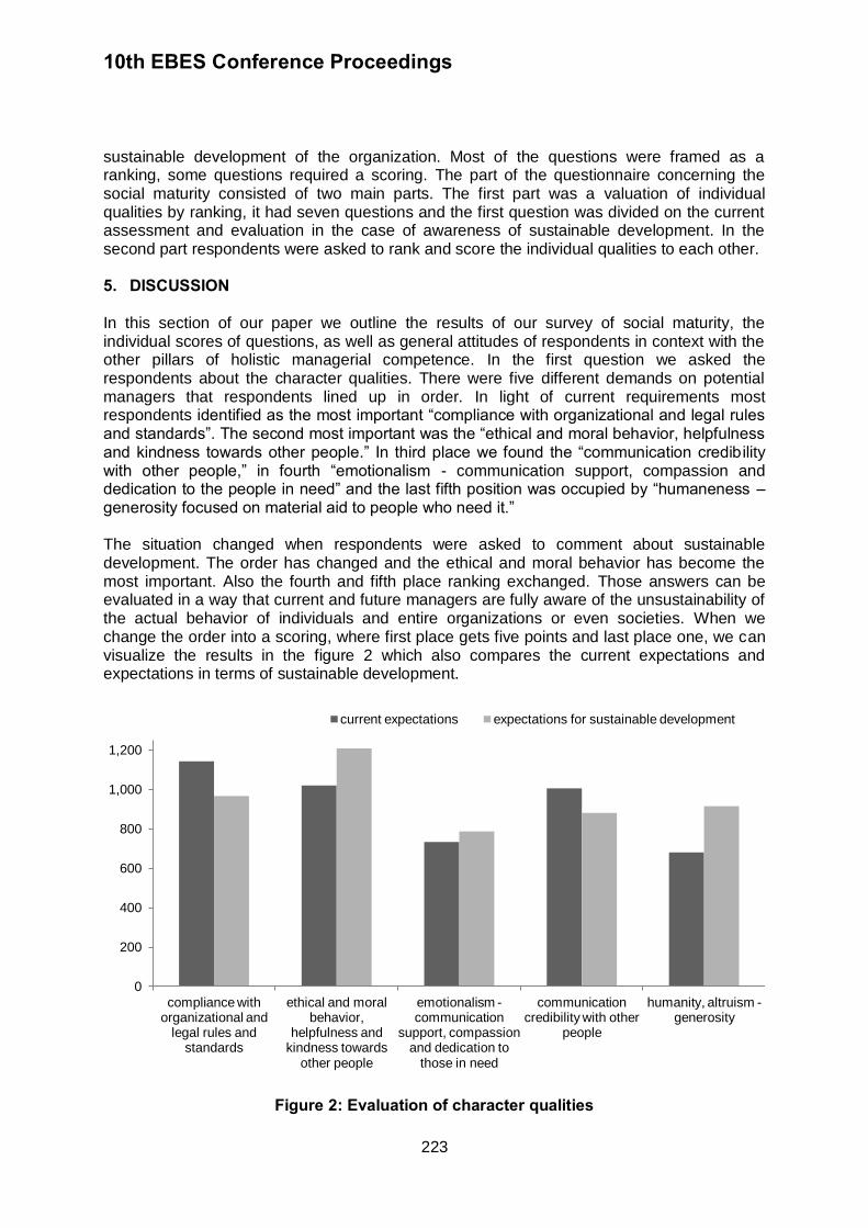
10th EBES Conference Proceedings
223
sustainable development of the organization. Most of the questions were framed as a ranking, some questions required a scoring. The part of the questionnaire concerning the social maturity consisted of two main parts. The first part was a valuation of individual qualities by ranking, it had seven questions and the first question was divided on the current assessment and evaluation in the case of awareness of sustainable development. In the second part respondents were asked to rank and score the individual qualities to each other. 5. DISCUSSION In this section of our paper we outline the results of our survey of social maturity, the individual scores of questions, as well as general attitudes of respondents in context with the other pillars of holistic managerial competence. In the first question we asked the respondents about the character qualities. There were five different demands on potential managers that respondents lined up in order. In light of current requirements most respondents identified as the most important “compliance with organizational and legal rules and standards”. The second most important was the “ethical and moral behavior, helpfulness and kindness towards other people.” In third place we found the “communication credib ility with other people,” in fourth “emotionalism - communication support, compassion and dedication to the people in need” and the last fifth position was occupied by “humaneness – generosity focused on material aid to people who need it.” The situation changed when respondents were asked to comment about sustainable development. The order has changed and the ethical and moral behavior has become the most important. Also the fourth and fifth place ranking exchanged. Those answers can be evaluated in a way that current and future managers are fully aware of the unsustainability of the actual behavior of individuals and entire organizations or even societies. When we change the order into a scoring, where first place gets five points and last place one, we can visualize the results in the figure 2 which also compares the current expectations and expectations in terms of sustainable development.
Figure 2: Evaluation of character qualities
0
200
400
600
800
1,000
1,200
compliance with organizational and
legal rules and standards
ethical and moral behavior,
helpfulness and kindness towards
other people
emotionalism - communication
support, compassion and dedication to
those in need
communication credibility with other
people
humanity, altruism - generosity
current expectations expectations for sustainable development
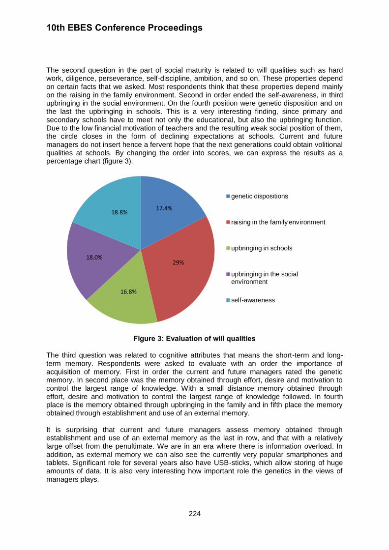
10th EBES Conference Proceedings
224
The second question in the part of social maturity is related to will qualities such as hard work, diligence, perseverance, self-discipline, ambition, and so on. These properties depend on certain facts that we asked. Most respondents think that these properties depend mainly on the raising in the family environment. Second in order ended the self-awareness, in third upbringing in the social environment. On the fourth position were genetic disposition and on the last the upbringing in schools. This is a very interesting finding, since primary and secondary schools have to meet not only the educational, but also the upbringing function. Due to the low financial motivation of teachers and the resulting weak social position of them, the circle closes in the form of declining expectations at schools. Current and future managers do not insert hence a fervent hope that the next generations could obtain volitional qualities at schools. By changing the order into scores, we can express the results as a percentage chart (figure 3).
Figure 3: Evaluation of will qualities The third question was related to cognitive attributes that means the short-term and long-term memory. Respondents were asked to evaluate with an order the importance of acquisition of memory. First in order the current and future managers rated the genetic memory. In second place was the memory obtained through effort, desire and motivation to control the largest range of knowledge. With a small distance memory obtained through effort, desire and motivation to control the largest range of knowledge followed. In fourth place is the memory obtained through upbringing in the family and in fifth place the memory obtained through establishment and use of an external memory. It is surprising that current and future managers assess memory obtained through establishment and use of an external memory as the last in row, and that with a relatively large offset from the penultimate. We are in an era where there is information overload. In addition, as external memory we can also see the currently very popular smartphones and tablets. Significant role for several years also have USB-sticks, which allow storing of huge amounts of data. It is also very interesting how important role the genetics in the views of managers plays.
17.4%
29%
16.8%
18.0%
18.8%
genetic dispositions
raising in the family environment
upbringing in schools
upbringing in the social environment
self-awareness
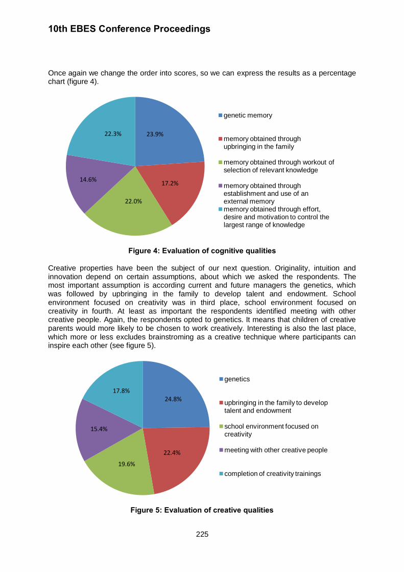
10th EBES Conference Proceedings
225
Once again we change the order into scores, so we can express the results as a percentage chart (figure 4).
Figure 4: Evaluation of cognitive qualities Creative properties have been the subject of our next question. Originality, intuition and innovation depend on certain assumptions, about which we asked the respondents. The most important assumption is according current and future managers the genetics, which was followed by upbringing in the family to develop talent and endowment. School environment focused on creativity was in third place, school environment focused on creativity in fourth. At least as important the respondents identified meeting with other creative people. Again, the respondents opted to genetics. It means that children of creative parents would more likely to be chosen to work creatively. Interesting is also the last place, which more or less excludes brainstroming as a creative technique where participants can inspire each other (see figure 5).
Figure 5: Evaluation of creative qualities
23.9%
17.2%
22.0%
14.6%
22.3%
genetic memory
memory obtained through upbringing in the family
memory obtained through workout of selection of relevant knowledge
memory obtained through establishment and use of an external memory memory obtained through effort, desire and motivation to control the largest range of knowledge
24.8%
22.4%
19.6%
15.4%
17.8%
genetics
upbringing in the family to develop talent and endowment
school environment focused on creativity
meeting with other creative people
completion of creativity trainings
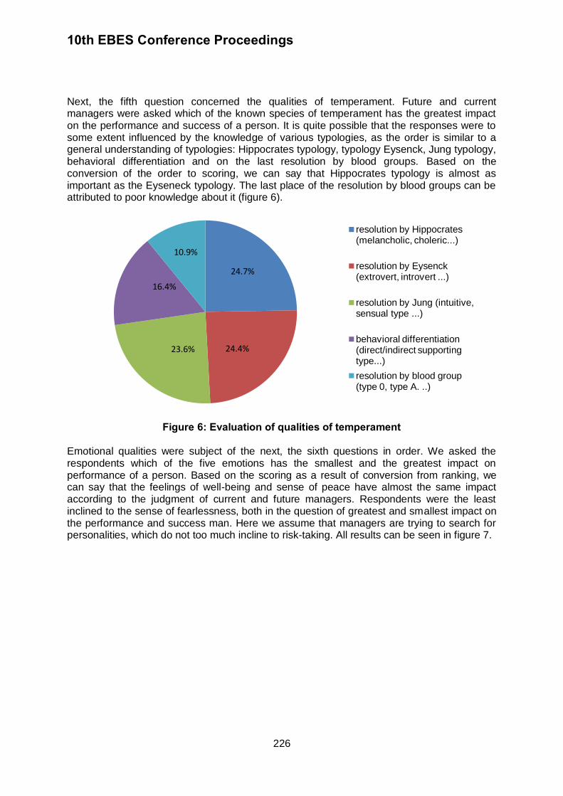
10th EBES Conference Proceedings
226
Next, the fifth question concerned the qualities of temperament. Future and current managers were asked which of the known species of temperament has the greatest impact on the performance and success of a person. It is quite possible that the responses were to some extent influenced by the knowledge of various typologies, as the order is similar to a general understanding of typologies: Hippocrates typology, typology Eysenck, Jung typology, behavioral differentiation and on the last resolution by blood groups. Based on the conversion of the order to scoring, we can say that Hippocrates typology is almost as important as the Eyseneck typology. The last place of the resolution by blood groups can be attributed to poor knowledge about it (figure 6).
Figure 6: Evaluation of qualities of temperament Emotional qualities were subject of the next, the sixth questions in order. We asked the respondents which of the five emotions has the smallest and the greatest impact on performance of a person. Based on the scoring as a result of conversion from ranking, we can say that the feelings of well-being and sense of peace have almost the same impact according to the judgment of current and future managers. Respondents were the least inclined to the sense of fearlessness, both in the question of greatest and smallest impact on the performance and success man. Here we assume that managers are trying to search for personalities, which do not too much incline to risk-taking. All results can be seen in figure 7.
24.7%
24.4% 23.6%
16.4%
10.9%
resolution by Hippocrates (melancholic, choleric...)
resolution by Eysenck (extrovert, introvert ...)
resolution by Jung (intuitive, sensual type ...)
behavioral differentiation (direct/indirect supporting type...)
resolution by blood group (type 0, type A. ..)
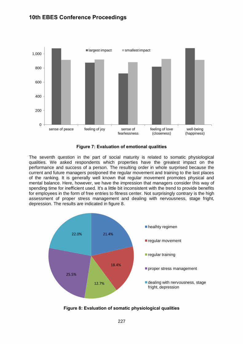
10th EBES Conference Proceedings
227
Figure 7: Evaluation of emotional qualities The seventh question in the part of social maturity is related to somatic physiological qualities. We asked respondents which properties have the greatest impact on the performance and success of a person. The resulting order in whole surprised because the current and future managers postponed the regular movement and training to the last places of the ranking. It is generally well known that regular movement promotes physical and mental balance. Here, however, we have the impression that managers consider this way of spending time for inefficient used. It's a little bit inconsistent with the trend to provide benefits for employees in the form of free entries to fitness center. Not surprisingly contrary is the high assessment of proper stress management and dealing with nervousness, stage fright, depression. The results are indicated in figure 8.
Figure 8: Evaluation of somatic physiological qualities
0
200
400
600
800
1,000
sense of peace feeling of joy sense of fearlessness
feeling of love (closeness)
well-being (happiness)
largest impact smallest impact
21.4%
18.4%
12.7%
25.5%
22.0%
healhty regimen
regular movement
regular training
proper stress management
dealing with nervousness, stage fright, depression
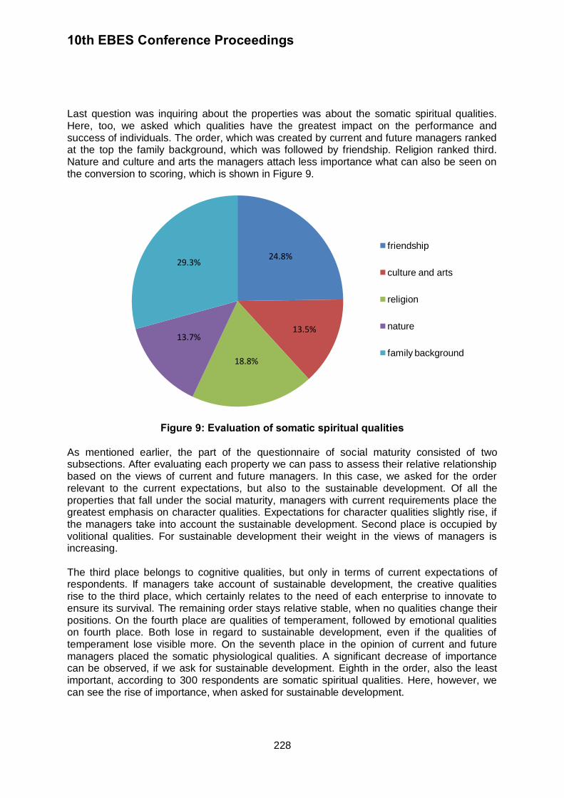
10th EBES Conference Proceedings
228
Last question was inquiring about the properties was about the somatic spiritual qualities. Here, too, we asked which qualities have the greatest impact on the performance and success of individuals. The order, which was created by current and future managers ranked at the top the family background, which was followed by friendship. Religion ranked third. Nature and culture and arts the managers attach less importance what can also be seen on the conversion to scoring, which is shown in Figure 9.
Figure 9: Evaluation of somatic spiritual qualities As mentioned earlier, the part of the questionnaire of social maturity consisted of two subsections. After evaluating each property we can pass to assess their relative relationship based on the views of current and future managers. In this case, we asked for the order relevant to the current expectations, but also to the sustainable development. Of all the properties that fall under the social maturity, managers with current requirements place the greatest emphasis on character qualities. Expectations for character qualities slightly rise, if the managers take into account the sustainable development. Second place is occupied by volitional qualities. For sustainable development their weight in the views of managers is increasing. The third place belongs to cognitive qualities, but only in terms of current expectations of respondents. If managers take account of sustainable development, the creative qualities rise to the third place, which certainly relates to the need of each enterprise to innovate to ensure its survival. The remaining order stays relative stable, when no qualities change their positions. On the fourth place are qualities of temperament, followed by emotional qualities on fourth place. Both lose in regard to sustainable development, even if the qualities of temperament lose visible more. On the seventh place in the opinion of current and future managers placed the somatic physiological qualities. A significant decrease of importance can be observed, if we ask for sustainable development. Eighth in the order, also the least important, according to 300 respondents are somatic spiritual qualities. Here, however, we can see the rise of importance, when asked for sustainable development.
24.8%
13.5%
18.8%
13.7%
29.3%
friendship
culture and arts
religion
nature
family background
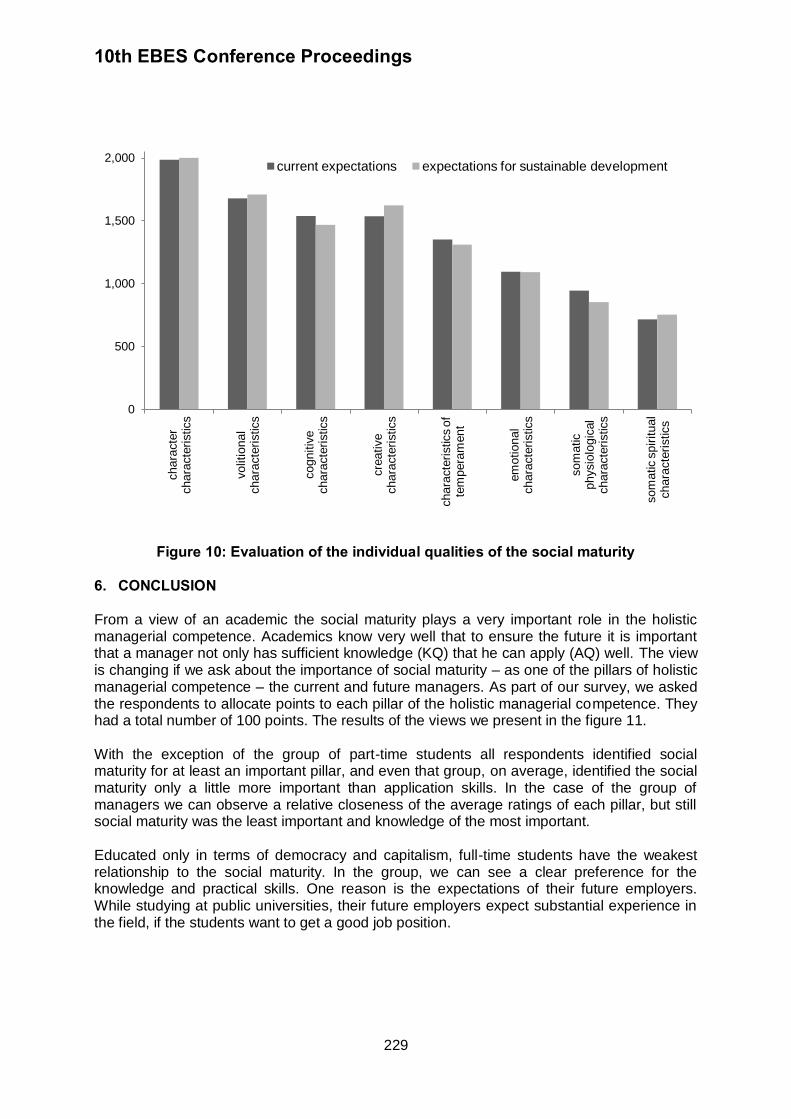
10th EBES Conference Proceedings
229
Figure 10: Evaluation of the individual qualities of the social maturity
6. CONCLUSION From a view of an academic the social maturity plays a very important role in the holistic managerial competence. Academics know very well that to ensure the future it is important that a manager not only has sufficient knowledge (KQ) that he can apply (AQ) well. The view is changing if we ask about the importance of social maturity – as one of the pillars of holistic managerial competence – the current and future managers. As part of our survey, we asked the respondents to allocate points to each pillar of the holistic managerial competence. They had a total number of 100 points. The results of the views we present in the figure 11. With the exception of the group of part-time students all respondents identified social maturity for at least an important pillar, and even that group, on average, identified the social maturity only a little more important than application skills. In the case of the group of managers we can observe a relative closeness of the average ratings of each pillar, but still social maturity was the least important and knowledge of the most important. Educated only in terms of democracy and capitalism, full-time students have the weakest relationship to the social maturity. In the group, we can see a clear preference for the knowledge and practical skills. One reason is the expectations of their future employers. While studying at public universities, their future employers expect substantial experience in the field, if the students want to get a good job position.
0
500
1,000
1,500
2,000 chara
cte
r chara
cte
ristics
volitional
chara
cte
ristics
cognitiv
e
chara
cte
ristics
cre
ative
chara
cte
ristics
chara
cte
ristics o
f te
mpera
ment
em
otional
chara
cte
ristics
som
atic
physio
logic
al
chara
cte
ristics
som
atic s
pir
itual
chara
cte
ristics
current expectations expectations for sustainable development
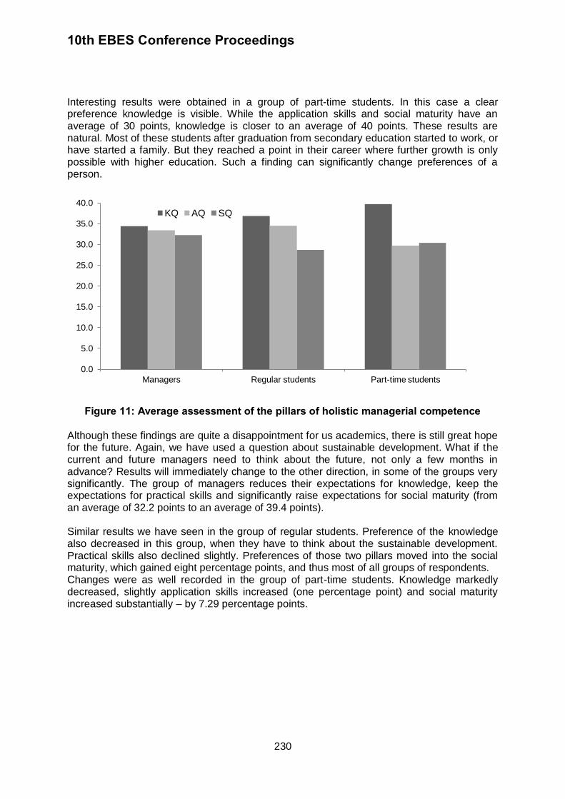
10th EBES Conference Proceedings
230
Interesting results were obtained in a group of part-time students. In this case a clear preference knowledge is visible. While the application skills and social maturity have an average of 30 points, knowledge is closer to an average of 40 points. These results are natural. Most of these students after graduation from secondary education started to work, or have started a family. But they reached a point in their career where further growth is only possible with higher education. Such a finding can significantly change preferences of a person.
Figure 11: Average assessment of the pillars of holistic managerial competence Although these findings are quite a disappointment for us academics, there is still great hope for the future. Again, we have used a question about sustainable development. What if the current and future managers need to think about the future, not only a few months in advance? Results will immediately change to the other direction, in some of the groups very significantly. The group of managers reduces their expectations for knowledge, keep the expectations for practical skills and significantly raise expectations for social maturity (from an average of 32.2 points to an average of 39.4 points). Similar results we have seen in the group of regular students. Preference of the knowledge also decreased in this group, when they have to think about the sustainable development. Practical skills also declined slightly. Preferences of those two pillars moved into the social maturity, which gained eight percentage points, and thus most of all groups of respondents. Changes were as well recorded in the group of part-time students. Knowledge markedly decreased, slightly application skills increased (one percentage point) and social maturity increased substantially – by 7.29 percentage points.
0.0
5.0
10.0
15.0
20.0
25.0
30.0
35.0
40.0
Managers Regular students Part-time students
KQ AQ SQ
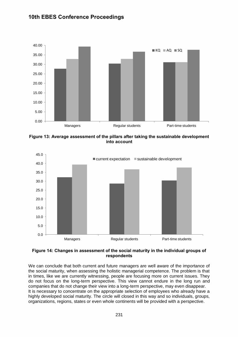
10th EBES Conference Proceedings
231
Figure 13: Average assessment of the pillars after taking the sustainable development into account
Figure 14: Changes in assessment of the social maturity in the individual groups of respondents
We can conclude that both current and future managers are well aware of the importance of the social maturity, when assessing the holistic managerial competence. The problem is that in times, like we are currently witnessing, people are focusing more on current issues. They do not focus on the long-term perspective. This view cannot endure in the long run and companies that do not change their view into a long-term perspective, may even disappear. It is necessary to concentrate on the appropriate selection of employees who already have a highly developed social maturity. The circle will closed in this way and so individuals, groups, organizations, regions, states or even whole continents will be provided with a perspective.
0.00
5.00
10.00
15.00
20.00
25.00
30.00
35.00
40.00
Managers Regular students Part-time students
KQ AQ SQ
0.0
5.0
10.0
15.0
20.0
25.0
30.0
35.0
40.0
45.0
Managers Regular students Part-time students
current expectation sustainable development

10th EBES Conference Proceedings
232
REFERENCES Albrecht, K., 2006. Social Intelligence. The new science of success. San Francisco: Jossey-
Bass. Birknerova, Z., Karas, L., and Ferencová, M. 2011. Socialne kompetencie v prostredi skoly [Social competences in the school environment]. In: Z. Birknerova ed. 2011. Socialna inteligencia v manazmente skoly a v pracovnom procese [Social intelligence in management of the school and in work]. Presov: Fakulta manazmentu, Presovska univerzita v Presove.
pp.29-37. Goleman, D., 2006. Social Inteligence: The revolutionary new science of human relationships. New York: Bantam Dell.
Hudakova, I. 2009. Lider ako osobnost a jeho kompetencie [Leader as a personality and his competences]. Dane & uctovnictvo, 14(9), pp.74-76.
Christopher, W.F., 2007. Holistic management – Managing what matters for company success. Hoboken: John Wiley & Sons.
Kosturiak, J., 2013. Leadership – navrat ke korenum. [Leadership – return to the roots]. Moderni rizeni. 48(2), pp.8-11.
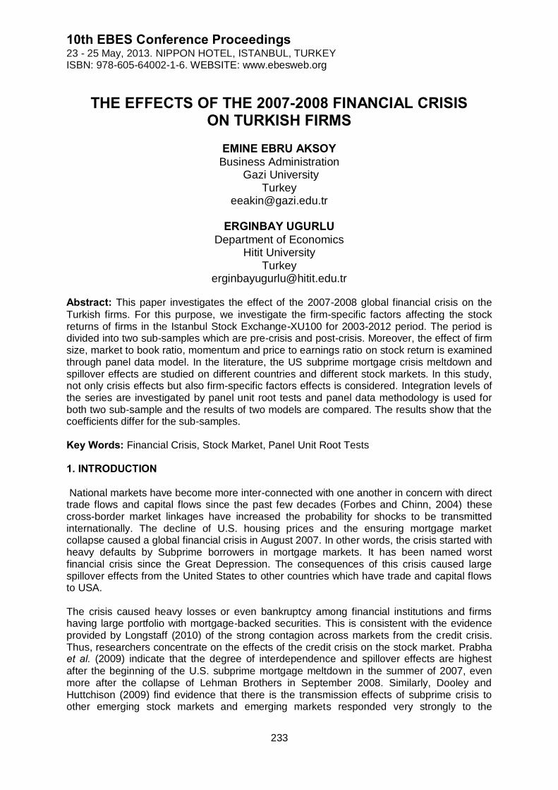
10th EBES Conference Proceedings 23 - 25 May, 2013. NIPPON HOTEL, ISTANBUL, TURKEY ISBN: 978-605-64002-1-6. WEBSITE: www.ebesweb.org
233
THE EFFECTS OF THE 2007-2008 FINANCIAL CRISIS ON TURKISH FIRMS
EMINE EBRU AKSOY
Business Administration Gazi University
Turkey [email protected]
ERGINBAY UGURLU
Department of Economics Hitit University
Turkey [email protected]
Abstract: This paper investigates the effect of the 2007-2008 global financial crisis on the
Turkish firms. For this purpose, we investigate the firm-specific factors affecting the stock returns of firms in the Istanbul Stock Exchange-XU100 for 2003-2012 period. The period is divided into two sub-samples which are pre-crisis and post-crisis. Moreover, the effect of firm size, market to book ratio, momentum and price to earnings ratio on stock return is examined through panel data model. In the literature, the US subprime mortgage crisis meltdown and spillover effects are studied on different countries and different stock markets. In this study, not only crisis effects but also firm-specific factors effects is considered. Integration levels of the series are investigated by panel unit root tests and panel data methodology is used for both two sub-sample and the results of two models are compared. The results show that the coefficients differ for the sub-samples. Key Words: Financial Crisis, Stock Market, Panel Unit Root Tests 1. INTRODUCTION National markets have become more inter-connected with one another in concern with direct trade flows and capital flows since the past few decades (Forbes and Chinn, 2004) these cross-border market linkages have increased the probability for shocks to be transmitted internationally. The decline of U.S. housing prices and the ensuring mortgage market collapse caused a global financial crisis in August 2007. In other words, the crisis started with heavy defaults by Subprime borrowers in mortgage markets. It has been named worst financial crisis since the Great Depression. The consequences of this crisis caused large spillover effects from the United States to other countries which have trade and capital flows to USA. The crisis caused heavy losses or even bankruptcy among financial institutions and firms having large portfolio with mortgage-backed securities. This is consistent with the evidence provided by Longstaff (2010) of the strong contagion across markets from the credit crisis. Thus, researchers concentrate on the effects of the credit crisis on the stock market. Prabha et al. (2009) indicate that the degree of interdependence and spillover effects are highest
after the beginning of the U.S. subprime mortgage meltdown in the summer of 2007, even more after the collapse of Lehman Brothers in September 2008. Similarly, Dooley and Huttchison (2009) find evidence that there is the transmission effects of subprime crisis to other emerging stock markets and emerging markets responded very strongly to the
10th EBES Conference Proceedings
234
deteriorating situation in the U.S. This study intends to analyze regarding the behavior of Turkish firms in term of the stock return, rather than the stock market. In this paper, we study whether and to what extent the subprime crisis spread from USA to Turkish economy. In this sense we analyze how stock return of Turkish firms listed in the ISE XU100 changed and which factors stimulated this change between 2003 -2012. Examining this variation across firms may offer us an entry into determining the extent to which the subprime crisis effects on the Turkish firms. Accordingly, we add two factors used by Fama and French (1992) which are firm size (log of assets), the ratio of the market to book values and we also add a third variable is momentum. It is interesting to know how Turkish firms’ stock return has been affected by the subprime crisis. The rest of paper is organized as follows: Section 2 includes some previous research outcomes related with stock returns. In the following section empirical application and main findings are represented. Section 4 concludes the paper. 2. LITERATURE REVIEW Examining the effects of the firms-specific factors on stock returns forms the basis of many studies. In the 1960s, the Capital Asset Pricing Model (CAPM) which is a single-factor model was developed by Treynor (1961, 1962), Sharpe (1964) and Lintner (1965). The model states that expected returns on stocks are positively related to market betas, and market betas are the only risk factor to explain the variation of expected return. On the other hand, Ross(1976) developed the Arbitrage Pricing Theory (APT) which is a multi-factor model. The theory is the idea that the expected return on stocks is driven by macro factors along with company specific factors. The theory is taken as a basis in the multi factor models to be developed for the further studies. With the widespread using of single factor and multi-factor models, several variables which are related with firms are discussed in different studies. Banz (1981) finds that average return is negatively regarding to firm size. In other words, smaller firms have higher risk adjusted returns on average than larger firms. Basu (1983) provides the evidence that the common stock of high earning/price firms gets higher risk adjusted returns than the common stock of low earning/price firms. On the other hand, the common stock of small firms earns higher returns than the common stock of large firms. Bhandari (1988) documents a positive relation between average return and the ratio of debt to equity. Chan et al. (1991) reveal that
there is a significant relation between earning yields, size, book-to-market ratio, cash flow yield and expected returns in the Japanese market. Moreover, the book-to-market ratio and cash flow yield have most significant positive impact on expected returns. The widely known studies about multi factor models are made by Fama and French. They try to find the factors describing the change in stock return. Fama and French (1992) confirm that size, earning-price, debt-equity and book-to-market ratios add to the explanation of expected stock return provided by market beta. Their main result is that size and book-to-market equity capture the cross-sectional variation in average stock returns associated with size, earning-price, book-to-market equity and leverage. They find that the relation between beta and average return is weak. Fama and French (1993) improve a three-factor model in which the factors are the market return in excess of the risk-free rate, the difference between the returns on small and large capitalization portfolios, and the difference between the returns on high and low book-to-market portfolios. They provide evidence that expected stock return can be explained by the excess market return, a size factor and a book-to-market equity factor. Fama and French (1995) show that high book to market equity firms
10th EBES Conference Proceedings
235
tend to be less earning than low book to market equity firms, and small stocks tend to be less earning than large stocks. Fama and French (1998), find that value stocks (high book-to-market ratio) have higher returns than growth stocks (low book-to-market ratio), and the average returns on global portfolios of high book-to-market stocks have higher than low book-to-market stocks. Chui and Wei (1998) investigate the relationship between expected stock returns and market beta, book-to-market equity, and size. They find that average stock return and market beta have a weak relationship. Moreover, the book-to-market equity can explain the cross-sectional variation of expected stock returns in Hong Kong, Korea, and Malaysia, and the size effect is significant in all markets except Taiwan. Some studies are conducted in order to examine the effects of firm’s specific factors on stock returns before and after the crisis period. Tong and Wei (2008) develop a methodology to study whether or how the financial sector crisis can spill over to the real economy. For this purpose, they investigate the relationship between stock returns and, demand sensitivity, financial constraint, size, market-to-book ratio, beta and momentum. They find that a tightened liquidity squeeze appears to be economically more important than reduced consumer confidence or spending in explaining cross-firm differences in stock price decline. In the same way, Tong and Wei (2009) study the relationship between stock return and demand sensitivity, financial dependence, size, market-to-book ratio, beta and momentum in the crisis period. They provide evidence that stock price performance is worse for firms with larger ex ante sensitivity to shocks to external finance, particularly in countries with rapid pre-crisis credit expansion. 3. EMPIRICAL APPLICATION In this paper, we study the effects of the 2007-2008 financial crisis on Turkish firms in the Istanbul Stock Exchange –XU100. For that purpose, we examine the effects of firm-specific factors which are firm size which is calculated as a log of total asset, market-to-book ratio, momentum and price to earnings ratio on stock return (percentage change in stock price) in 2003:01-2013:02 period for monthly data. The model is follows:
(1)
where j is index for firm, t is index for time period (month), STC is stock return, SIZE is firm size, BMV is market-to-book ratio, MOM is momentum and PE is price to earnings ratio . We have deleted the firms with missing data and firms which have outliers especially on market-to-book value. The final sample consists of 59 firms (see: Appendix ) which gives the total of 7198 observations. However full sample period is broken up into sub-samples which are named pre-crisis (2003:01-2007:05) and post-crisis (2008:05 to 2013:02) periods. The subprime crisis period is defined as July 31, 2007 – March 31, 2008 by Tong and Wei (2009) . In this paper same period with Tong and Wei (2009) taken as a crisis period in this paper. The omitting observations are calculated by adding two months after crisis period and subtracting two months before crisis period thus we have 2007:06-2008:03 period to be deleted. Figure shows the stock return against time for 59 firms. There are some peaks for majority of firms that are 2006:01, between 2007:01- 2008:01 and between 2009:01-2010:01 periods.
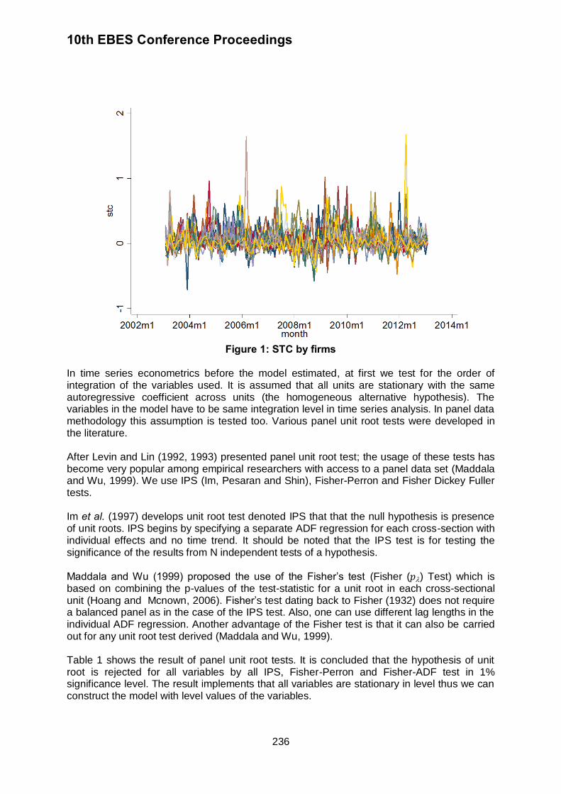
10th EBES Conference Proceedings
236
Figure 1: STC by firms
In time series econometrics before the model estimated, at first we test for the order of integration of the variables used. It is assumed that all units are stationary with the same autoregressive coefficient across units (the homogeneous alternative hypothesis). The variables in the model have to be same integration level in time series analysis. In panel data methodology this assumption is tested too. Various panel unit root tests were developed in the literature. After Levin and Lin (1992, 1993) presented panel unit root test; the usage of these tests has become very popular among empirical researchers with access to a panel data set (Maddala and Wu, 1999). We use IPS (Im, Pesaran and Shin), Fisher-Perron and Fisher Dickey Fuller tests. Im et al. (1997) develops unit root test denoted IPS that that the null hypothesis is presence of unit roots. IPS begins by specifying a separate ADF regression for each cross-section with individual effects and no time trend. It should be noted that the IPS test is for testing the significance of the results from N independent tests of a hypothesis.
Maddala and Wu (1999) proposed the use of the Fisher’s test (Fisher ( ) Test) which is based on combining the p-values of the test-statistic for a unit root in each cross-sectional unit (Hoang and Mcnown, 2006). Fisher’s test dating back to Fisher (1932) does not require a balanced panel as in the case of the IPS test. Also, one can use different lag lengths in the individual ADF regression. Another advantage of the Fisher test is that it can also be carried out for any unit root test derived (Maddala and Wu, 1999). Table 1 shows the result of panel unit root tests. It is concluded that the hypothesis of unit root is rejected for all variables by all IPS, Fisher-Perron and Fisher-ADF test in 1% significance level. The result implements that all variables are stationary in level thus we can construct the model with level values of the variables.

10th EBES Conference Proceedings
237
Table 1 : Panel unit root test Results: Full Sample Variable STC SIZE BMV MOM
Im-Pesaran-Shin
Without Trend
-81.7170*** -4.3016*** -11.8950 *** -81.9667*** -27.6203***
With Trend -84.1988*** -4.3892*** -9.7340*** -84.4629*** -25.6542***
Fisher-Perron Test
Without Trend
Inverse Inverse normal Inverse logit Modified inv. Pm
4209.6355 *** -62.0498*** -151.3314*** 266.3428 ***
237.4499*** -4.6423*** - 5.3141*** 7.7755***
477.9401 *** -11.3835*** -15.4952 *** 23.4301***
4209.6355*** -62.0498 *** -151.3314*** 266.3428***
1045.4143*** -26.1934*** -37.2671*** 60.3695***
With Trend
Inverse Inverse normal Inverse logit Modified inv. Pm
4096.5742 *** -61.1115*** -147.2670*** 258.9831 ***
190.2354*** -4.4276*** -4.4161*** 4.7021***
373.6137*** -8.9165 *** -11.5763*** 16.6390 ***
4096.5742 *** -61.1115*** -147.2670*** 258.9831***
856.6378*** -22.8232*** -30.4501*** 48.0812***
Fisher- ADF Test
Without Trend
Inverse Inverse normal Inverse logit Modified inv. Pm
1282.8093*** -31.2546*** -46.1145 *** 75.8226***
320.9766 *** -7.5323*** -8.9117*** 13.2126***
343.0988*** -9.1261 *** -10.4607*** 14.6527***
1278.4798*** -31.2335*** -45.9590*** 75.5408***
1282.8093*** -31.2546*** -46.1145*** 75.8226***
With Trend
Inverse Inverse normal Inverse logit Modified inv. Pm
1052.2227 *** -27.5130 *** -37.8208 *** 60.8127 ***
283.6968 *** -7.7265 *** -8.2512*** 10.7859***
271.0662*** -7.2967 *** -7.8048 *** 9.9638***
1047.9032*** -27.4832*** -37.6658*** 60.5315***
1052227*** -27.5130*** -37.8208*** 60.8127***
Note: *,**,*** show 10%, 5% and 1% significance respectively. The p value of the test when the null hypothesis of unit root is not rejected is in bold. Automatic selection of lags based on the Akaike Information Criterion. In Fisher type 3 lags option is selected.
Although we investigated the order of integration of MOM we estimated following model (equation 2). Because we had very high R-squared value (0.67) and peculiar results which can be sing of multicollinearity then we omitted the MOM variable from the model. We use the model by taking in consider Fama-French (1992) which is follows: (2)
Table 2 shows panel data estimation results of both full sample and two sub-samples. Whereas for sub-sample1 and sub-sample2 Hausman test concludes REM for full-sample null hypothesis of the test is rejected and FEM is chosen. R-squared of the models are low but except full-sample REM model is not significant all models are statistically significant. FEM model of full-sample is significant in %5 significance level, all other significant models is significant in %1 significance level.
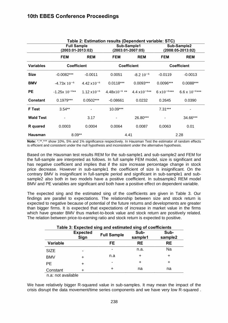
10th EBES Conference Proceedings
238
Table 2: Estimation results (Dependent variable: STC)
Full Sample
(2003:01-2013:02) Sub-Sample1
(2003:01-2007:05) Sub-Sample2
(2008:05-2013:02)
FEM REM FEM REM FEM REM
Variables Coefficient Coefficient Coefficient
Size -0.0082*** -0.0011 0.0051 -8.2 -0.0119 -0.0013
BMV -4.73x 4.42 x 0.0118*** 0.0093*** 0.0096*** 0.0088***
PE -1.25x ** 1.12 x 4.48x ** 4.4 x ** 6 x *** 6.6 x ***
Constant 0.1979*** 0.0502*** -0.08661 0.0232 0.2645 0.0390
F Test 3.54** - 10.09*** 7.31*** -
Wald Test - 3.17 - 26.80*** - 34.66***
R quared 0.0003 0.0004 0.0064 0.0087 0,0063 0.01
Hausman 8.09** 4.41 2.28
Note: *,**,*** show 10%, 5% and 1% significance respectively. In Hausman Test the estimator of random effects is efficient and consistent under the null hypothesis and inconsistent under the alternative hypothesis.
Based on the Hausman test results REM for the sub-sample1 and sub-sample2 and FEM for the full-sample are interpreted as follows. In full sample FEM model, size is significant and has negative coefficient and implies that if the size increase percentage change in stock price decrease. However in sub-sample1 the coefficient of size is insignificant. On the contrary BMV is insignificant in full-sample period and significant in sub-sample1 and sub-sample2 also both in two models have a positive coefficient. In subsample2 REM model BMV and PE variables are significant and both have a positive effect on dependent variable. The expected sing and the estimated sing of the coefficients are given in Table 3. Our findings are parallel to expectations. The relationship between size and stock return is expected to negative because of potential of the future returns and developments are greater than bigger firms. It is expected that expectations of increase in market value in the firms which have greater BMV thus market-to-book value and stock return are positively related. The relation between price-to-earning ratio and stock return is expected to positive.
Table 3: Expected sing and estimated sing of coefficients
Expected Sign Full Sample Sub-
sample1 Sub-
sample2 Variable FE RE RE
SIZE - - n.a. Na
BMV + n.a + +
PE + - + +
Constant + + na na
n.a: not available We have relatively bigger R-squared value in sub-samples. It may mean the impact of the crisis disrupt the data movement/time series components and we have very low R-squared .
10th EBES Conference Proceedings
239
But if we split the sample for sub-samples we have more consistent data for the investigated period. Although PE variable has negative effect in full-sample that contradiction with expectation, has positive sing in sub-samples parallel to expectation. 4. CONCLUSION This paper empirically investigates the 2007 financial crisis whether has the effects of on Turkish firms. To investigate this 2003:01-2013:02 monthly data is used and the data period considers both pre-crisis and post-crisis period. To represent Turkish firms Istanbul Stock Exchange –XU100 are selected to collect data. After many arrangements on the data we have 59 Turkish firms in XU100. The variables used are stock return as a dependent variable and firm size, market-to-book ratio, momentum and price-to-earning ratio variables as independents. The models are estimated for three different samples. First we used full sample then full sample period was divided into sub-samples which are pre-crisis and post-crisis periods then models are estimated and interpreted for both subsamples. We have two main findings which show us effect of independent variables on stock return and differentiation of effects of sample and sub-sample against each other. The findings show that size has a negatively, market-to-book ratio has positively, and price-to-earning ratio has related with stock return and the results are different for the samples. Hence we conclude that the crisis has effect on Turkish firms. We suggest that to use more independent variables and more firms from different markets for future researches. REFERENCES Banz, R.W., 1981. The relationship between return and market value of common stocks. Journal of Financial Economics, 9(1), pp.3-18. Basu, S.,1983. The relationship between earnings’ yield, market value and return for NYSE common stocks. Journal of Financial Economics, 12(1), pp.129-156 Bhandari, L.C., 1988. Debt/Equity ratio and expected common stock returns: Empirical evidence. Journal of Finance, 43(2), pp.507-528
Chan, K.C.L., Hamao, Y., and Lakonishok,J. 1991. Fundamentals and stock returns in Japan. The Journal of Finance, 46(5), pp.1739-1764 Chui, A.C.W. and Wei, J.K.C., 1998. Book-to-Market, firm size, and the Turn-of-The-Year Effect: Evidence from Pacific-Basin emerging market. Pacific-Basin Finance Journal, 6(3-4), pp.275-293 Dooley, M. and Hutchison, M., 2009. Transmission of the U.S. subprime crisis to emerging markets: Evidence on the Decoupling-Recoupling hypothesis. Journal of International Money and Finance, 28(8), pp.1331-1349. Fama, E.F. and French, K.R., 1992. The cross-section of expected stock returns. The Journal of Finance, 47(2), pp.427-465. Fama, E.F. and French, K.R., 1993. Common risk factors in the returns on stocks and bonds. Journal of Financial Economics, 33(1), pp.3-56.

10th EBES Conference Proceedings
240
Fama, E.F. and French, K.R., 1995. Size and book-to-market factors in earnings and returns. The Journal of Finance, 50(1), pp.131-155 Fama, E.F. and French, K.R., 1998. Value versus growth: The international evidence. The Journal of Finance, 53(6), pp.1975-1999 Fisher, R.A., 1932. Statistical methods for research workers. Edinburgh: Oliver & Boyd. Forbes, K.J. and Chinn, M.D., 2004. A decomposition of global linkages in financial markets over time. The Review of Economics and Statistics, 86(3) pp.705-722. Hoang, N. T. and McNown R. F., 2006 Panel data unit roots tests using various estimation methods. Working Paper, Department of Economics, University of Colorado at Boulder. Im, K.S., Pesaran, M.H. and Shin, Y., 1997. Testing for unit roots in heterogeneous panels, Mimeo, Department of Applied Economics, University of Cambridge. Lintner, J., 1965. The Valuation of risk assets and the selection of risky investments in stock portfolios and capital budgets. The Review of Economics and Statistics, 47(1), pp.13-37.
Longstaff, F.A., 2010. The subprime credit crisis and contagion in financial markets, Journal of Financial Economics, 97(3), pp.436-450. Maddala, G.S. and Wu, S., 1999. A comparative study of unit root tests with panel data and a new simple test. Oxford Bulletin of Economics and Statistics, 61(3), pp.631-652. Prabha, A.P.A., Barth, J.R., and Kim, H., 2009. Spillover Effects from the U.S. financial crisis: Some time-series evidence from national stock returns. In: B.E. Gup, ed. The Financial and Economic Crisis: An International Perspective. UK: Edward Elgar Publishing. Ross, A.S., 1976. The Arbitrage Theory of capital asset pricing, Journal of Economic Theory,
13(3), pp.341-360. Sharpe, W.F., 1964. Capital asset prices: A theory of market equilibrium under conditions of risk. Journal of Finance, 19(3), pp.425-442. Tong, H. and Wei, S. J., 2008. Real effects of the subprime Mortgage crisis: Is it a demand or a finance shock? NBER Working Paper Series, 14205 Tong, H. and Wei, S.J., 2009. Real effects of The 2007-2008 financial crisis around the world. [online] Available at: <http://papers.ssrn.com/sol3/papers.cfm?abstract_id=1363819>
[Accessed 1 May 2013] Treynor, J.L., 1961. Market value, time, and risk. Unpublished Manuscript Treynor, J.L., 1962. Toward a theory of market value of risky assets. Unpublished Manuscript.

10th EBES Conference Proceedings
241
APPENDIX
List of Firms AEFES 1 AYGAZ 11 EREGL 21
AFYON 2 BAGFS 12 FROTO 22
AKBNK 3 BANVT 13 GARAN 23
AKENR 4 BRISA 14 GOLTS 24
AKSA 5 BRSAN 15 GOODY 25
ALGYO 6 CLEBI 16 GSDHO 26
ALKIM 7 ECILC 17 GUBRF 27
ARCLK 8 ECZYT 18 HURGZ 28
ASELS 9 EGEEN 19 IHEVA 29
ASUZU 10 EGGUB 20 IHLAS 30
IPEKE 31 METRO 40 SKBNK 50
ISCTR 32 MGROS 41 TCELL 51
ISGYO 33 NETAS 42 TEBNK 52
IZMDC 34 NTHOL 43 THYAO 53
KARSN 35 OTKAR 44 TIRE 54
KARTN 36 PETKM 45 TOASO 55
KCHOL 37 PRKME 46 TRCAS 56
KCHOL 37 SAHOL 47 TRKCM 57
KONYA 38 SASA 48 TUPRS 58
KRDMD 39 SISE 49 VESTL 59
10th EBES Conference Proceedings 23 - 25 May, 2013. NIPPON HOTEL, ISTANBUL, TURKEY ISBN: 978-605-64002-1-6. WEBSITE: www.ebesweb.org
242
CHINA’S APPEARING ON THE HORIZON AND THE CHANGING PATTERN OF GLOBAL ECONOMY
XUHENG ZANG Institute of Consumption & Development
Shandong University P. R. China
YANG LI Institute of Consumption & Development
Shandong University P. R. China
YANG HE Institute of Consumption & Development
Shandong University P. R. China
Abstract: Since the new century, especially so for the past five years, the particular striking
matter in the world is that the pattern of the global economy as a whole is changing. The developed countries are suffering a financial crisis and economic depression, the BRICS countries are rising and having fast economic booming, especially China is experiencing a rapid economic rise, which all marks a new global economic growth pattern formation. The paper re-analyzed the basis of two round migrations of the world's centers of economic growth in modern economic history, and points out the third round of economic growth centers are formed but has not yet been completed. It is necessary to recognize this global economic growth pattern in the future, and understand properly the impact and consequences of the third round of economic growth centers. It is analyzed the symbols of the fact that the rise of China, mainly resulting in the change of the global economic pattern, as well as the main features of the new pattern. The global economic structure and pattern in 2020 are expected to be: dual master countries (that is both China and United States) drive and multi-centers pattern. Keywords: Economic Growth Centers, Rise Of China, Global Economic Pattern
1. INTRODUCTION In modern economic history, there are two rounds migrations of the world's centers of economic growth: the first round began after opening up new routes and it transfers from the Mediterranean coast to the Atlantic coast. As a result, the United Kingdom grew to become the economic center of the world. The second round began from the late of 19th century and the world economic center shifts from the United Kingdom to the United States. So far, in the short term, no country can shake the U.S. leading economic power. However, since the new century, especially after the global financial crisis in 2008, the global economic pattern began a far-reaching change. The developed countries are suffering a financial crisis and economic depression, the BRICS countries are rising and having fast economic booming, especially China is experiencing a rapid economic rise, which all marks a new global economic growth

10th EBES Conference Proceedings
243
pattern formation. The paper re-analyzed the basis of two round migrations of the world's centers of economic growth in modern economic history, and points out the third round of economic growth centers are formed but has not yet been completed. It is necessary to recognize this global economic growth pattern in the future, and understand properly the impact and consequences of the third round of economic growth centers. It is analyzed the symbols of the fact that the rise of China including the overall economic strength, innovation and technological progress, industrial production, foreign trade and changes in the economic structure, mainly resulting in the change of the global economic pattern, as well as the main features of the new pattern. The global economic structure and pattern in 2020 are expected to be: dual master countries (that is both China and United States) drive and multi-centers pattern (Madison, 2001). The remainder of this paper is structured as follows. In Part Two, we re-analyzed the basis of two round migrations of the world's centers of economic growth in modern economic history, especially economic symbols in the process. In Part Three, we discuss the facts and influence of the rise of China. In Part Four, we analyses changes of economic status and the global economy and point out that China's economic development has brought development opportunities for Asia and the world. 2. TWO ROUND MIGRATIONS OF THE WORLD’S CENTERS OF ECONOMIC GROWTH IN MODERN ECONOMIC HISTORY 2.1. Industrial revolution in British At the end of the 16th century, Italy and the Mediterranean region which had been the center of world science and technology since the Renaissance began to decline gradually with the discovery of new travel routes. From the beginning of the 17th century to 1830, the center for world economy gradually shifted from Italy to the UK. The Industrial Revolution, which began in the first in the latter half of 17th century, had the economy shifted from agriculture, handicraft economy to economy with industrial and machine production dominated, promoted the economic, social, political and cultural transformation, and established the UK as the "world factory" ( Wilson, 1977).
2.1.1. Britain became world's industrial center
The great achievements of the Industrial Revolution, promoted the substantial production growth in major industrial sectors in Britain, mainly in the textile industry, metallurgical industry, machinery manufacturing and other aspects. In 1810, half a century after the beginning of the Industrial Revolution, the textile industry of the UK has a monopoly position in the world. In the early 1820s, number of spindles owned by Britain was 3-4 times more than that of France, and 10 times more than Germany. In the metallurgical industry, the production of British’s pig iron increased to 2.29 million tons producing 50.9% of the world's iron, which was twice of the total production of France, Russia, the United States and Germany. In latter 19th century and early 20th century, British’s coal production was more than 14 million tons, while the coal production in France and Prussia was about 1 million tons separately. The United States only produced 50-60 thousand tons. In 1850, British’s coal production was more than 50 million tons, while the total production of France, the U.S. and Germany was only a little more than one third of Britain’s production. In 1820, Britain’s gross industrial product was half of that of the world, which was far more than other countries. In 1840, the industrial production of Britain accounted for 45% in the world, while

10th EBES Conference Proceedings
244
France was 12%, the United States 11%. Britain still occupied the dominant position in world industrial production until the 1870s. In 1870, Britain’s coal mining accounted for 51.5% in the world and pig iron production accounted for 50%, the cotton consumption 49.2%. Its national income was much higher than its neighbors in terms of population. According to statistics, the per capita annual income of British citizens in 1860 was 32.6 pounds, while France was 21.1 pounds in 1859; Germany was 13.3 pounds on average from 1860 to1869.
2.1.2. The technical superiority of Britain By the mid-19th century, the technology in European continent was an era behind that of the Britain. In the 1820s, coal had already been used for pig-iron smelting instead of charcoal in Britain, while iron making with charcoal was still dominating in other countries. At the same period, most of the cotton mills were manual or animal powered in France and Germany. In machine manufacturing, almost all the steam engines were from the United Kingdom in the 18th century. Before the mid-19th century, few of the machines produced in the European continent were exported, and machine manufacturing scale was much smaller than that in the United Kingdom. 2.1.3. Monopoly on world trade Britain has occupied a pivotal position in the establishing period of international trade. During the period from 1801 to 1850 after the Industrial Revolution, the export volume valuated by the British official increased from 24.9 million pounds to 175.4 million pounds, increased by more than 600%. In 1850, UK accounted for 22% of the total world trade. In 1821-1873, the annual growth rate of per capita export volume was 4.3%, which was about three times of the per capita income growth rate (1.57%). In 1870, the proportion of Britain’s trade volume in total world trade volume increased to 25%. It was almost equivalent to the sum total of France, Germany, and the United States. 2.1.4. Pound’s status in world currency The growth of the capital market in the UK and the expansion of Britain’s foreign trade promoted the rapid growth of London’s importance as world center of commerce and finance. From the 19th century, London has overtaken Amsterdam, Hamburg and Paris and became the financial center of Europe and even the world. Many foreign banks established branches in London. After 1870, the number of bank branches expanded rapidly. These banks mainly engaged in foreign exchange business. It is also during this period that pound gradually became an international currency in the London capital market. 2.2. The industrialization of the United States The Industrialization in the United States is half a century behind that of the Britain. But it developed rapidly and promoted the U.S to become the world's top industrial powers quickly. In the late 19th century, the United States began the second Industrial Revolution, and finished first in the world the shift from the “Age of Steam” and “Mechanical Age" to the "Age of Electrification", "oil era", "Iron Age", from light industry country to heavy industry country (Gunderson, 1976). The second Industrial Revolution in the United States first began in energy sector. There were more than 500 Ac power stations in American by 1892 and 2774 in 1898. From the year 1876 when Bell invented the telephone, the United States has 1.355 million units of telephones by 1980 and to 10 million units in 1914. The electricity consumption in 1924 reached 65 billion
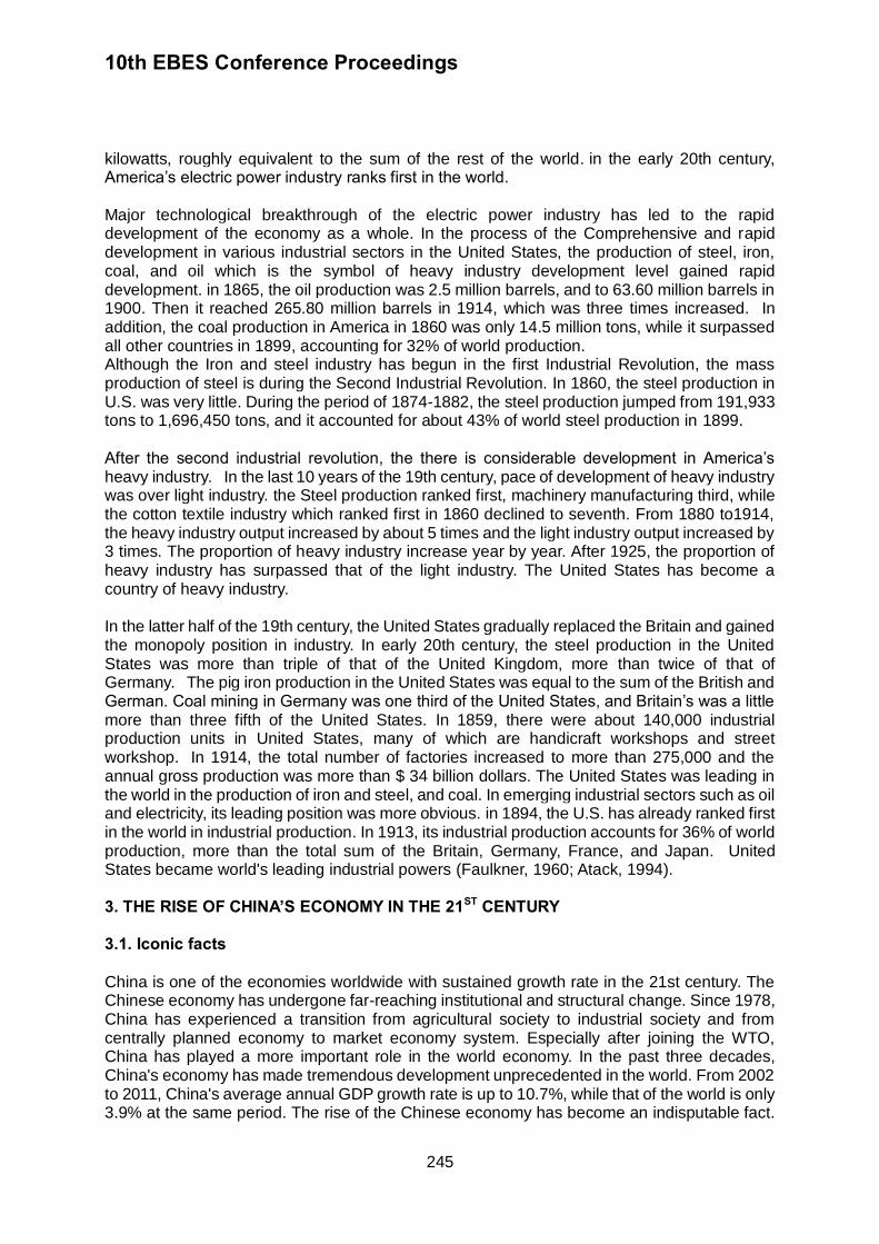
10th EBES Conference Proceedings
245
kilowatts, roughly equivalent to the sum of the rest of the world. in the early 20th century, America’s electric power industry ranks first in the world. Major technological breakthrough of the electric power industry has led to the rapid development of the economy as a whole. In the process of the Comprehensive and rapid development in various industrial sectors in the United States, the production of steel, iron, coal, and oil which is the symbol of heavy industry development level gained rapid development. in 1865, the oil production was 2.5 million barrels, and to 63.60 million barrels in 1900. Then it reached 265.80 million barrels in 1914, which was three times increased. In addition, the coal production in America in 1860 was only 14.5 million tons, while it surpassed all other countries in 1899, accounting for 32% of world production. Although the Iron and steel industry has begun in the first Industrial Revolution, the mass production of steel is during the Second Industrial Revolution. In 1860, the steel production in U.S. was very little. During the period of 1874-1882, the steel production jumped from 191,933 tons to 1,696,450 tons, and it accounted for about 43% of world steel production in 1899. After the second industrial revolution, the there is considerable development in America’s heavy industry. In the last 10 years of the 19th century, pace of development of heavy industry was over light industry. the Steel production ranked first, machinery manufacturing third, while the cotton textile industry which ranked first in 1860 declined to seventh. From 1880 to1914, the heavy industry output increased by about 5 times and the light industry output increased by 3 times. The proportion of heavy industry increase year by year. After 1925, the proportion of heavy industry has surpassed that of the light industry. The United States has become a country of heavy industry. In the latter half of the 19th century, the United States gradually replaced the Britain and gained the monopoly position in industry. In early 20th century, the steel production in the United States was more than triple of that of the United Kingdom, more than twice of that of Germany. The pig iron production in the United States was equal to the sum of the British and German. Coal mining in Germany was one third of the United States, and Britain’s was a little more than three fifth of the United States. In 1859, there were about 140,000 industrial production units in United States, many of which are handicraft workshops and street workshop. In 1914, the total number of factories increased to more than 275,000 and the annual gross production was more than $ 34 billion dollars. The United States was leading in the world in the production of iron and steel, and coal. In emerging industrial sectors such as oil and electricity, its leading position was more obvious. in 1894, the U.S. has already ranked first in the world in industrial production. In 1913, its industrial production accounts for 36% of world production, more than the total sum of the Britain, Germany, France, and Japan. United States became world's leading industrial powers (Faulkner, 1960; Atack, 1994). 3. THE RISE OF CHINA’S ECONOMY IN THE 21ST CENTURY 3.1. Iconic facts China is one of the economies worldwide with sustained growth rate in the 21st century. The Chinese economy has undergone far-reaching institutional and structural change. Since 1978, China has experienced a transition from agricultural society to industrial society and from centrally planned economy to market economy system. Especially after joining the WTO, China has played a more important role in the world economy. In the past three decades, China's economy has made tremendous development unprecedented in the world. From 2002 to 2011, China's average annual GDP growth rate is up to 10.7%, while that of the world is only 3.9% at the same period. The rise of the Chinese economy has become an indisputable fact.
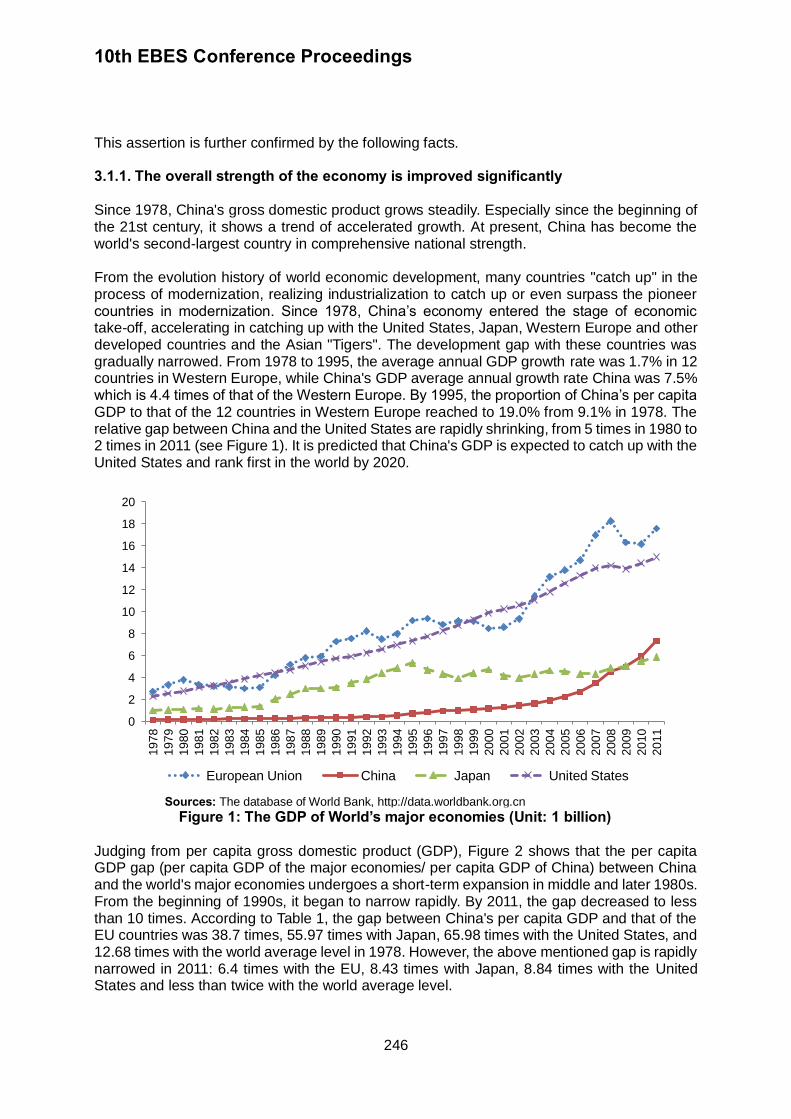
10th EBES Conference Proceedings
246
This assertion is further confirmed by the following facts.
3.1.1. The overall strength of the economy is improved significantly Since 1978, China's gross domestic product grows steadily. Especially since the beginning of the 21st century, it shows a trend of accelerated growth. At present, China has become the world's second-largest country in comprehensive national strength. From the evolution history of world economic development, many countries "catch up" in the process of modernization, realizing industrialization to catch up or even surpass the pioneer countries in modernization. Since 1978, China’s economy entered the stage of economic take-off, accelerating in catching up with the United States, Japan, Western Europe and other developed countries and the Asian "Tigers". The development gap with these countries was gradually narrowed. From 1978 to 1995, the average annual GDP growth rate was 1.7% in 12 countries in Western Europe, while China's GDP average annual growth rate China was 7.5% which is 4.4 times of that of the Western Europe. By 1995, the proportion of China’s per capita GDP to that of the 12 countries in Western Europe reached to 19.0% from 9.1% in 1978. The relative gap between China and the United States are rapidly shrinking, from 5 times in 1980 to 2 times in 2011 (see Figure 1). It is predicted that China's GDP is expected to catch up with the United States and rank first in the world by 2020.
Sources: The database of World Bank, http://data.worldbank.org.cn
Figure 1: The GDP of World’s major economies (Unit: 1 billion) Judging from per capita gross domestic product (GDP), Figure 2 shows that the per capita GDP gap (per capita GDP of the major economies/ per capita GDP of China) between China and the world's major economies undergoes a short-term expansion in middle and later 1980s. From the beginning of 1990s, it began to narrow rapidly. By 2011, the gap decreased to less than 10 times. According to Table 1, the gap between China's per capita GDP and that of the EU countries was 38.7 times, 55.97 times with Japan, 65.98 times with the United States, and 12.68 times with the world average level in 1978. However, the above mentioned gap is rapidly narrowed in 2011: 6.4 times with the EU, 8.43 times with Japan, 8.84 times with the United States and less than twice with the world average level.
0
2
4
6
8
10
12
14
16
18
20
1978
1979
1980
1981
1982
1983
1984
1985
1986
1987
1988
1989
1990
1991
1992
1993
1994
1995
1996
1997
1998
1999
2000
2001
2002
2003
2004
2005
2006
2007
2008
2009
2010
2011
European Union China Japan United States
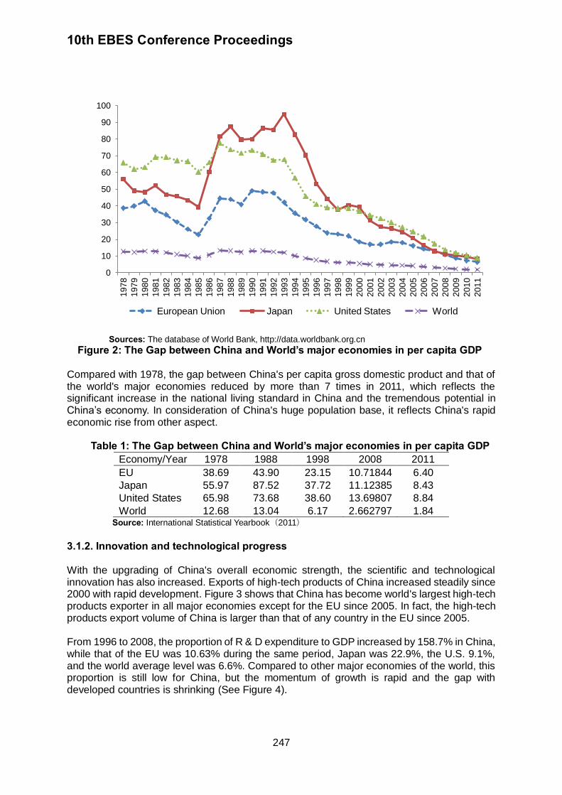
10th EBES Conference Proceedings
247
Sources: The database of World Bank, http://data.worldbank.org.cn
Figure 2: The Gap between China and World’s major economies in per capita GDP
Compared with 1978, the gap between China's per capita gross domestic product and that of the world's major economies reduced by more than 7 times in 2011, which reflects the significant increase in the national living standard in China and the tremendous potential in China’s economy. In consideration of China's huge population base, it reflects China's rapid economic rise from other aspect.
Table 1: The Gap between China and World’s major economies in per capita GDP
Economy/Year 1978 1988 1998 2008 2011
EU 38.69 43.90 23.15 10.71844 6.40
Japan 55.97 87.52 37.72 11.12385 8.43
United States 65.98 73.68 38.60 13.69807 8.84
World 12.68 13.04 6.17 2.662797 1.84 Source: International Statistical Yearbook(2011) 3.1.2. Innovation and technological progress With the upgrading of China's overall economic strength, the scientific and technological innovation has also increased. Exports of high-tech products of China increased steadily since 2000 with rapid development. Figure 3 shows that China has become world's largest high-tech products exporter in all major economies except for the EU since 2005. In fact, the high-tech products export volume of China is larger than that of any country in the EU since 2005. From 1996 to 2008, the proportion of R & D expenditure to GDP increased by 158.7% in China, while that of the EU was 10.63% during the same period, Japan was 22.9%, the U.S. 9.1%, and the world average level was 6.6%. Compared to other major economies of the world, this proportion is still low for China, but the momentum of growth is rapid and the gap with developed countries is shrinking (See Figure 4).
0
10
20
30
40
50
60
70
80
90
100
1978
1979
1980
1981
1982
1983
1984
1985
1986
1987
1988
1989
1990
1991
1992
1993
1994
1995
1996
1997
1998
1999
2000
2001
2002
2003
2004
2005
2006
2007
2008
2009
2010
2011
European Union Japan United States World
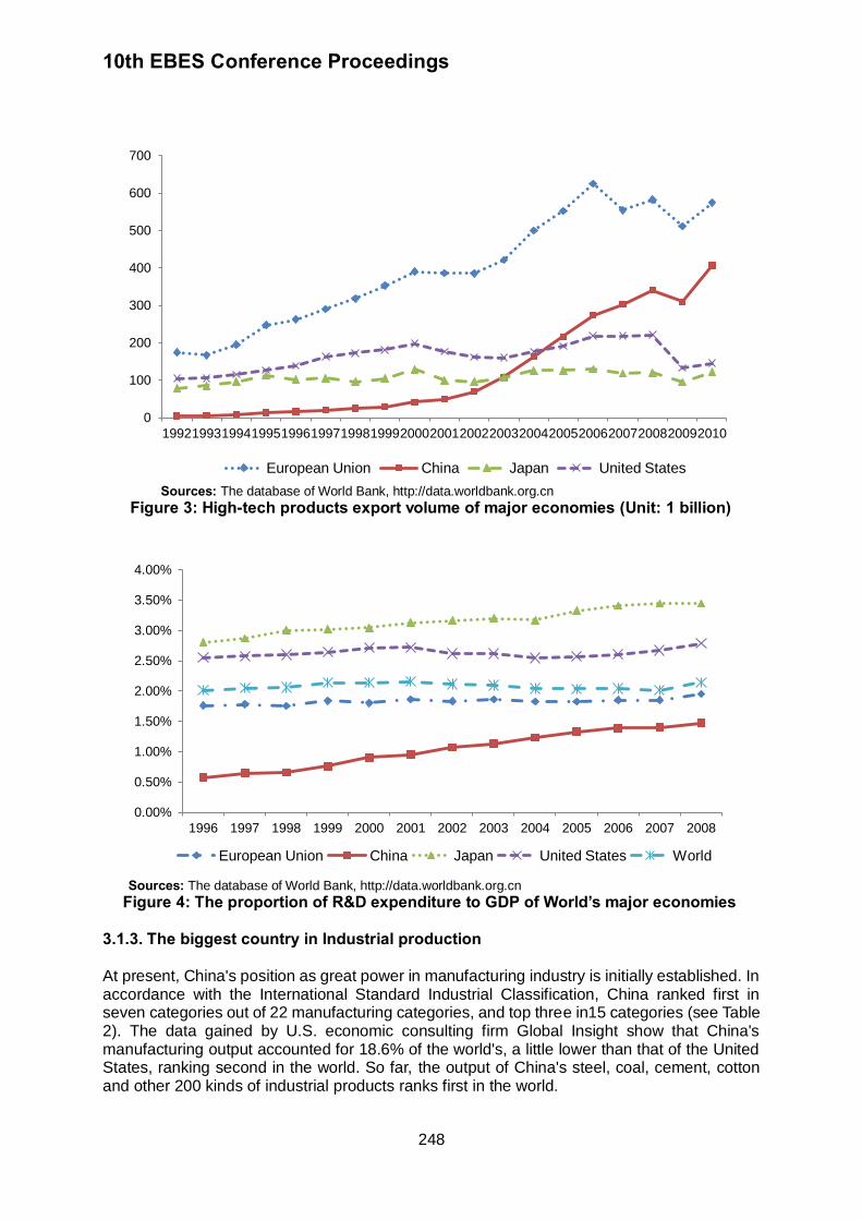
10th EBES Conference Proceedings
248
Sources: The database of World Bank, http://data.worldbank.org.cn
Figure 3: High-tech products export volume of major economies (Unit: 1 billion)
Sources: The database of World Bank, http://data.worldbank.org.cn
Figure 4: The proportion of R&D expenditure to GDP of World’s major economies 3.1.3. The biggest country in Industrial production At present, China's position as great power in manufacturing industry is initially established. In accordance with the International Standard Industrial Classification, China ranked first in seven categories out of 22 manufacturing categories, and top three in15 categories (see Table 2). The data gained by U.S. economic consulting firm Global Insight show that China's manufacturing output accounted for 18.6% of the world's, a little lower than that of the United States, ranking second in the world. So far, the output of China's steel, coal, cement, cotton and other 200 kinds of industrial products ranks first in the world.
0
100
200
300
400
500
600
700
1992 1993 1994 1995 1996 1997 1998 1999 2000 2001 2002 2003 2004 2005 2006 2007 2008 2009 2010
European Union China Japan United States
0.00%
0.50%
1.00%
1.50%
2.00%
2.50%
3.00%
3.50%
4.00%
1996 1997 1998 1999 2000 2001 2002 2003 2004 2005 2006 2007 2008
European Union China Japan United States World

10th EBES Conference Proceedings
249
Table 2: The rank of China’s main product output in the World Item 1978 1980 1990 2000 2008 2009 2010
Crude Steel 5 5 4 2 1 1 1
Coal 3 3 1 1 1 1 Crude Oil 8 6 5 5 5 4 4
Electric Energy Production 7 6 4 2 2 2 1
Cement 4 4 1 1 1 1 1
Fertilizer 3 3 3 1 1 1 Cotton 1 1 1 2 1 1 1
Sources: International Statistical Yearbook(2011)
3.1.4. Foreign trade In 1978, the proportion of China's total volume of foreign trade to the world is less than 1%, ranking 29th in the world. In 2009, the amount of China's exports surpassed that of Germany and ranked first in the world. The amount of import ranked second. .In 2010, f China's total volume of foreign trade was up to 2.9728 trillion U.S. dollars, making a record high (see Table 3).
Table 3: The total volume of foreign trade of World’s major economies
(Unit: 100 million dollars) Country/Year 2000 2005 2007 2008 2009 2010
China 4743 14219 21766 25633 22075 29729
Japan 8588 11108 13366 15439 11327 14625
America 20412 26338 31686 34569 26613 32462
France 6666 9676 11905 13314 10447 11264
Germany 10490 17480 23762 26312 20464 23360
Italy 4793 7579 10115 11047 8220 9318
Britain 6335 8981 10620 10926 8357 9622
Australia 1354 2314 3067 3875 3198 4141 Sources: WTO Database
3.1.5. Changes in economic structure Table 4 shows the proportion of the added value of agriculture, industry and services industry to GDP in world's major countries. Compared with the data of 2000, the proportion of the added value of agriculture decreased by y 5.6%; the proportion of the industrial added value remained roughly the same; and the added value of service industry increased by 6.9%. The changes in industrial structure were greater than world’s other major countries and the world average level, which shows that China's economy is going through a transition period, and the industrial structure is becoming more rational.
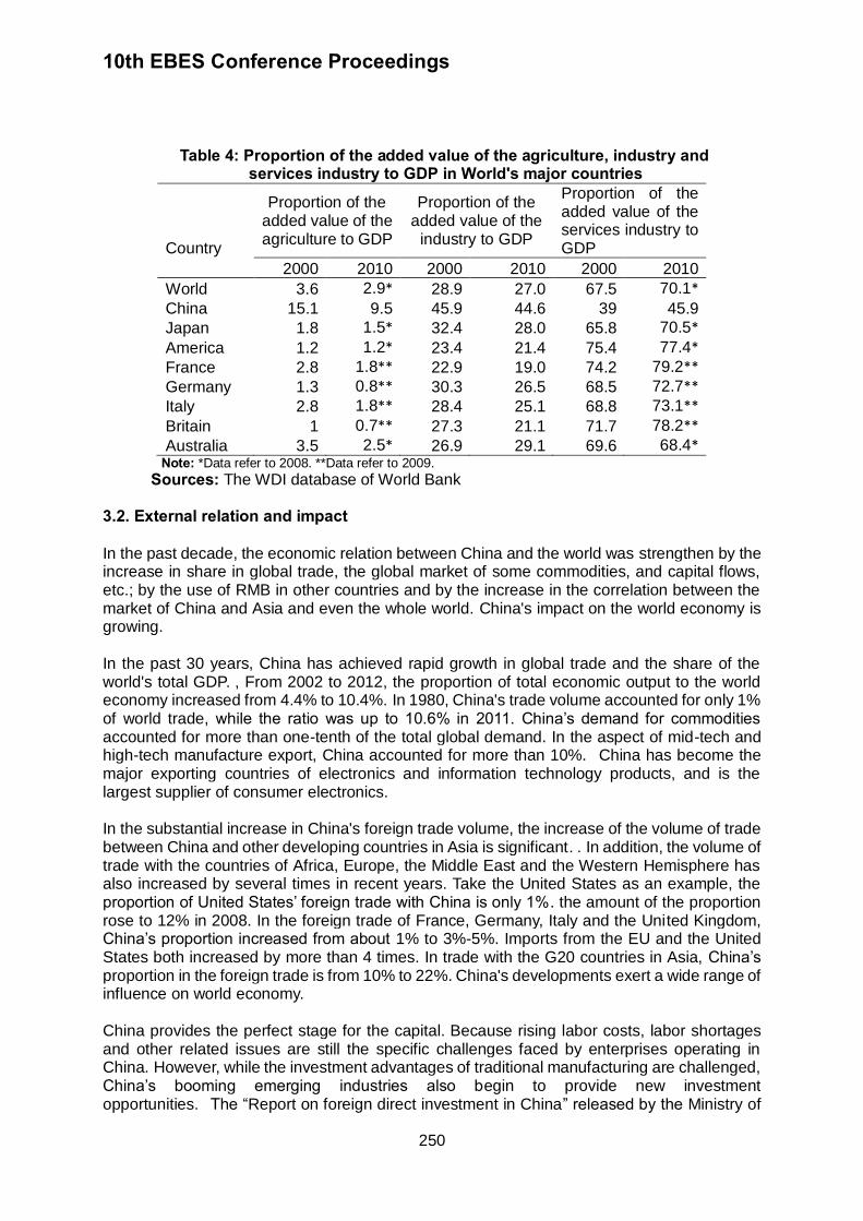
10th EBES Conference Proceedings
250
Table 4: Proportion of the added value of the agriculture, industry and services industry to GDP in World's major countries
Country
Proportion of the added value of the agriculture to GDP
Proportion of the added value of the
industry to GDP
Proportion of the added value of the services industry to GDP
2000 2010 2000 2010 2000 2010
World 3.6 2.9* 28.9 27.0 67.5 70.1*
China 15.1 9.5 45.9 44.6 39 45.9
Japan 1.8 1.5* 32.4 28.0 65.8 70.5*
America 1.2 1.2* 23.4 21.4 75.4 77.4*
France 2.8 1.8** 22.9 19.0 74.2 79.2**
Germany 1.3 0.8** 30.3 26.5 68.5 72.7**
Italy 2.8 1.8** 28.4 25.1 68.8 73.1**
Britain 1 0.7** 27.3 21.1 71.7 78.2**
Australia 3.5 2.5* 26.9 29.1 69.6 68.4* Note: *Data refer to 2008. **Data refer to 2009.
Sources: The WDI database of World Bank
3.2. External relation and impact In the past decade, the economic relation between China and the world was strengthen by the increase in share in global trade, the global market of some commodities, and capital flows, etc.; by the use of RMB in other countries and by the increase in the correlation between the market of China and Asia and even the whole world. China's impact on the world economy is growing. In the past 30 years, China has achieved rapid growth in global trade and the share of the world's total GDP. , From 2002 to 2012, the proportion of total economic output to the world economy increased from 4.4% to 10.4%. In 1980, China's trade volume accounted for only 1% of world trade, while the ratio was up to 10.6% in 2011. China’s demand for commodities accounted for more than one-tenth of the total global demand. In the aspect of mid-tech and high-tech manufacture export, China accounted for more than 10%. China has become the major exporting countries of electronics and information technology products, and is the largest supplier of consumer electronics. In the substantial increase in China's foreign trade volume, the increase of the volume of trade between China and other developing countries in Asia is significant. . In addition, the volume of trade with the countries of Africa, Europe, the Middle East and the Western Hemisphere has also increased by several times in recent years. Take the United States as an example, the proportion of United States’ foreign trade with China is only 1%. the amount of the proportion rose to 12% in 2008. In the foreign trade of France, Germany, Italy and the United Kingdom, China’s proportion increased from about 1% to 3%-5%. Imports from the EU and the United States both increased by more than 4 times. In trade with the G20 countries in Asia, China’s proportion in the foreign trade is from 10% to 22%. China's developments exert a wide range of influence on world economy. China provides the perfect stage for the capital. Because rising labor costs, labor shortages and other related issues are still the specific challenges faced by enterprises operating in China. However, while the investment advantages of traditional manufacturing are challenged, China’s booming emerging industries also begin to provide new investment opportunities. The “Report on foreign direct investment in China” released by the Ministry of
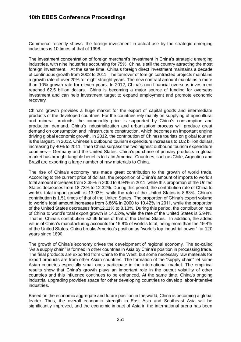
10th EBES Conference Proceedings
251
Commerce recently shows: the foreign investment in actual use by the strategic emerging industries is 10 times of that of 1998. The investment concentration of foreign merchant’s investment in China’s strategic emerging industries, with nine industries accounting for 75%. China is still the country attracting the most foreign investment. At the same time, China's foreign direct investment maintains a decade of continuous growth from 2002 to 2011. The turnover of foreign contracted projects maintains a growth rate of over 20% for eight straight years. The new contract amount maintains a more than 10% growth rate for eleven years. In 2012, China's non-financial overseas investment reached 62.5 billion dollars. China is becoming a major source of funding for overseas investment and can help investment target to expand employment and promote economic recovery. China's growth provides a huge market for the export of capital goods and intermediate products of the developed countries. For the countries rely mainly on supplying of agricultural and mineral products, the commodity price is supported by China's consumption and production demand. China's industrialization and urbanization process will produce great demand on consumption and infrastructure construction, which becomes an important engine driving global economic growth. In 2012, the contribution of Chinese tourists on global tourism is the largest. In 2012, Chinese’s outbound tourism expenditure increases to 102 billion dollars, increasing by 40% to 2011. Then China surpass the two highest outbound tourism expenditure countries--- Germany and the United States. China’s purchase of primary products in global market has brought tangible benefits to Latin America. Countries, such as Chile, Argentina and Brazil are exporting a large number of raw materials to China. The rise of China's economy has made great contribution to the growth of world trade. According to the current price of dollars, the proportion of China’s amount of imports to world’s total amount increases from 3.35% in 2000 to 9.94% in 2011, while this proportion of the United States decreases from 18.73% to 12.32%. During this period, the contribution rate of China to world’s total import growth is 13.03%, while the rate of the United States is 8.63%. China’s contribution is 1.51 times of that of the United States. The proportion of China’s export volume to world’s total amount increases from 3.86% in 2000 to 10.42% in 2011, wh ile the proportion of the United States decreases from12.11% to 8.13%. During this period, the contribution rate of China to world’s total export growth is 14.02%, while the rate of the United States is 5.94%. That is, China’s contribution is2.36 times of that of the United States. In addition, the added value of China’s manufacturing accounts for 19.8% of world's total, being more than the 19.4% of the United States. China breaks America’s position as “world’s top industrial power” for 120 years since 1890. The growth of China’s economy drives the development of regional economy. The so-called “Asia supply chain” is formed in other countries in Asia by China’s position in processing trade. The final products are exported from China to the West, but some necessary raw materials for export products are from other Asian countries. The formation of the "supply chain" let some Asian countries especially small ones participate in the international market. The empirical results show that China's growth plays an important role in the output volatility of other countries and this influence continues to be enhanced. At the same time, China's ongoing industrial upgrading provides space for other developing countries to develop labor-intensive industries. Based on the economic aggregate and future position in the world, China is becoming a global leader. Thus, the overall economic strength in East Asia and Southeast Asia will be significantly improved, and the economic impact of Asia in the international arena has been
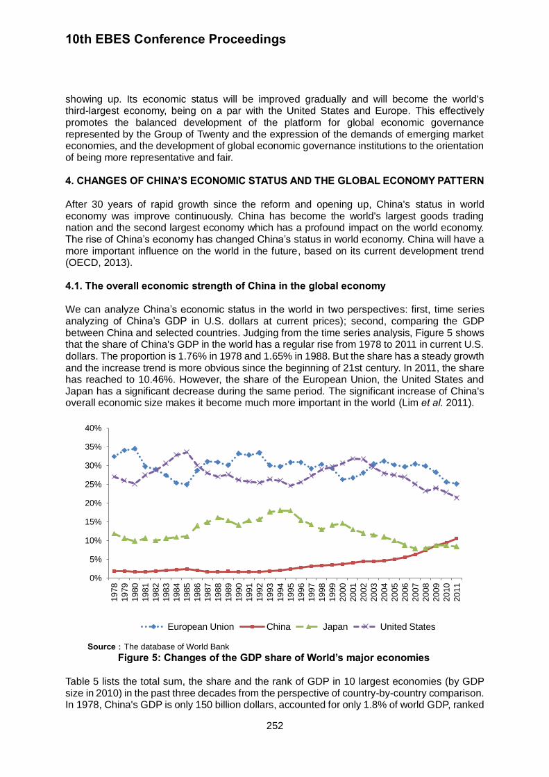
10th EBES Conference Proceedings
252
showing up. Its economic status will be improved gradually and will become the world's third-largest economy, being on a par with the United States and Europe. This effectively promotes the balanced development of the platform for global economic governance represented by the Group of Twenty and the expression of the demands of emerging market economies, and the development of global economic governance institutions to the orientation of being more representative and fair.
4. CHANGES OF CHINA’S ECONOMIC STATUS AND THE GLOBAL ECONOMY PATTERN After 30 years of rapid growth since the reform and opening up, China's status in world economy was improve continuously. China has become the world's largest goods trading nation and the second largest economy which has a profound impact on the world economy. The rise of China’s economy has changed China’s status in world economy. China will have a more important influence on the world in the future, based on its current development trend (OECD, 2013).
4.1. The overall economic strength of China in the global economy We can analyze China’s economic status in the world in two perspectives: first, time series analyzing of China’s GDP in U.S. dollars at current prices); second, comparing the GDP between China and selected countries. Judging from the time series analysis, Figure 5 shows that the share of China's GDP in the world has a regular rise from 1978 to 2011 in current U.S. dollars. The proportion is 1.76% in 1978 and 1.65% in 1988. But the share has a steady growth and the increase trend is more obvious since the beginning of 21st century. In 2011, the share has reached to 10.46%. However, the share of the European Union, the United States and Japan has a significant decrease during the same period. The significant increase of China's overall economic size makes it become much more important in the world (Lim et al. 2011).
Source:The database of World Bank
Figure 5: Changes of the GDP share of World’s major economies Table 5 lists the total sum, the share and the rank of GDP in 10 largest economies (by GDP size in 2010) in the past three decades from the perspective of country-by-country comparison. In 1978, China's GDP is only 150 billion dollars, accounted for only 1.8% of world GDP, ranked
0%
5%
10%
15%
20%
25%
30%
35%
40%
1978
1979
1980
1981
1982
1983
1984
1985
1986
1987
1988
1989
1990
1991
1992
1993
1994
1995
1996
1997
1998
1999
2000
2001
2002
2003
2004
2005
2006
2007
2008
2009
2010
2011
European Union China Japan United States
10th EBES Conference Proceedings
253
10th in the world, which is vastly disproportionate with the status of the world's most populous country. Though China had maintained a rapid economic growth, the share of GDP in the world economy is only 3.7% in 2000, lagging behind in Japan, Germany, Britain, France and other traditional developed countries. The ranking improved to No.6, but the international influence is still limited. Since the beginning of 21st century, this situation has undergone significant changes. China’s GDP has exceeded that of France, Britain, Germany and Japan, and becomes the world's second largest economy just behind the United States. In 2012, China's GDP reached 7.2 trillion U.S. dollars, accounting for more than 12% of the world GDP and becoming a significantly influential economy.
Table 5: GDP of World’s major economies since 1978
Country
2010 2000 1978
Sort
GDP (billion dollars)
Share ( %)
Sort GDP
(billion dollars)
Share ( %)
sort GDP
(billion dollars)
Share ( %)
United States 1 14.59 23.1 1 9.90 30.7 1 2.28 27.1
China 2 5.93 9.4 6 1.20 3.7 10 0.15 1.8
Japan 3 5.46 8.6 2 4.67 14.5 2 0.98 11.7
Germany 4 3.28 5.2 3 1.89 5.9 3 0.72 8.5 France 5 2.56 4.1 5 1.33 4.1 4 0.50 5.9
United Kingdom 6 2.25 3.6 4 1.48 4.6 5 0.33 3.9
Brazil 7 2.09 3.3 9 0.64 2.0 8 0.20 2.4
Italy 8 2.05 3.2 7 1.10 3.4 6 0.30 3.6
India 9 1.73 2.7 13 0.46 1.4 13 0.14 1.6
Canada 10 1.58 2.5 8 0.72 2.2 7 0.21 2.6
World 63.12 100 32.24 100 8.42 100
Source:The database of World Bank
Table 5 also shows changes of GDP and its share of world’s other major economies. It also shows the rising of China’s economic status compared with the group of developed countries and emerging countries group. Developed countries can be divided into three groups since 1978: the global GDP share of countries in the first groups (including the United States, Japan and the United Kingdom) increases in the first 20 years and decreases in recent 10 years; the global GDP share of Canada which represents the second group declines in the first 20 years and increases from 2.2% to 2.5% in nearly 10 year; the third group (including Germany, France and Italy) declines continuously. Take the United States and Japan for example, The GDP share of the United States is 27.1% in 1978 and up to 30.7% in 2000. The new technological revolution, financial and cultural industries innovation and the development of real estate, has contributed to the economic growth of the United States and the world during this period. The share declined to 23.1%, a decrease by 7.6% though its economy continued to grow in the last ten years. The GDP share of Japan was 11.7% in 1978 and reach 14.5% in 2000. However, the share declines to 8.6% from 14.5% in the last 10 years. The share of countries of the Group of Seven all declines in the past 30 years. Among them, the United States decreases by 4%, Japan decreases by 3.1%, Germany decreases by 3.3%. However, the share of China increases to 7.6% during this period and exceeds the sum of the amount changes in both the United States and Japan that have the most closely economic and trade relations with China. This also explains why the world is becoming increasingly concerned about the development of China.
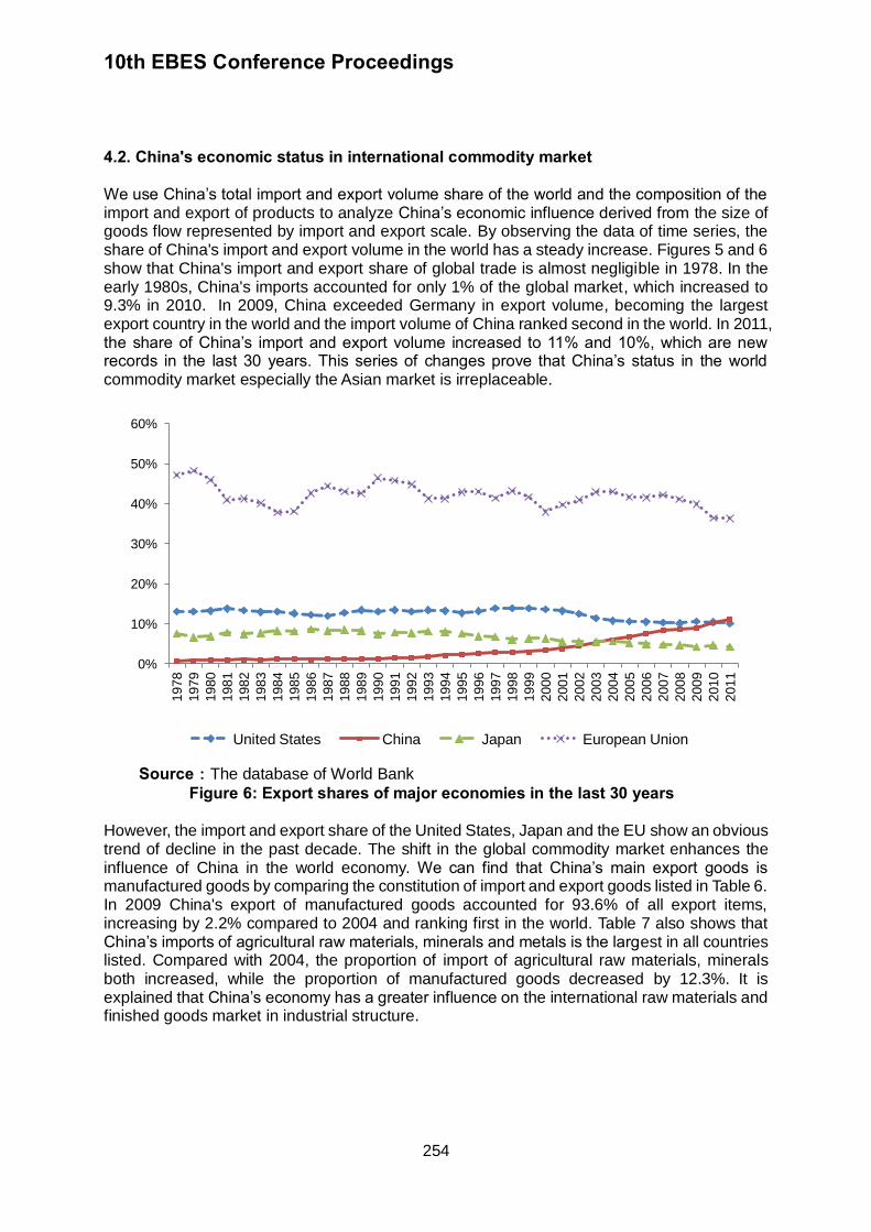
10th EBES Conference Proceedings
254
4.2. China's economic status in international commodity market We use China’s total import and export volume share of the world and the composition of the import and export of products to analyze China’s economic influence derived from the size of goods flow represented by import and export scale. By observing the data of time series, the share of China's import and export volume in the world has a steady increase. Figures 5 and 6 show that China's import and export share of global trade is almost negligible in 1978. In the early 1980s, China's imports accounted for only 1% of the global market, which increased to 9.3% in 2010. In 2009, China exceeded Germany in export volume, becoming the largest export country in the world and the import volume of China ranked second in the world. In 2011, the share of China’s import and export volume increased to 11% and 10%, which are new records in the last 30 years. This series of changes prove that China’s status in the world commodity market especially the Asian market is irreplaceable.
Source:The database of World Bank
Figure 6: Export shares of major economies in the last 30 years However, the import and export share of the United States, Japan and the EU show an obvious trend of decline in the past decade. The shift in the global commodity market enhances the influence of China in the world economy. We can find that China’s main export goods is manufactured goods by comparing the constitution of import and export goods listed in Table 6. In 2009 China's export of manufactured goods accounted for 93.6% of all export items, increasing by 2.2% compared to 2004 and ranking first in the world. Table 7 also shows that China’s imports of agricultural raw materials, minerals and metals is the largest in all countries listed. Compared with 2004, the proportion of import of agricultural raw materials, minerals both increased, while the proportion of manufactured goods decreased by 12.3%. It is explained that China’s economy has a greater influence on the international raw materials and finished goods market in industrial structure.
0%
10%
20%
30%
40%
50%
60%
1978
1979
1980
1981
1982
1983
1984
1985
1986
1987
1988
1989
1990
1991
1992
1993
1994
1995
1996
1997
1998
1999
2000
2001
2002
2003
2004
2005
2006
2007
2008
2009
2010
2011
United States China Japan European Union
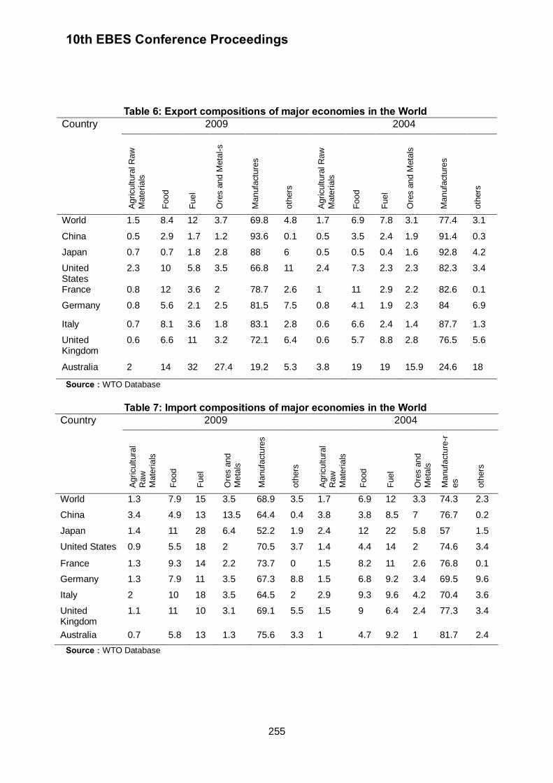
10th EBES Conference Proceedings
255
Table 6: Export compositions of major economies in the World
Country 2009 2004 A
gricultura
l R
aw
M
ate
rials
Food
Fuel
Ore
s a
nd M
eta
l-s
Manufa
ctu
res
oth
ers
Agricultura
l R
aw
Mate
rials
Food
Fuel
Ore
s a
nd M
eta
ls
Manufa
ctu
res
oth
ers
World 1.5 8.4 12 3.7 69.8 4.8 1.7 6.9 7.8 3.1 77.4 3.1
China 0.5 2.9 1.7 1.2 93.6 0.1 0.5 3.5 2.4 1.9 91.4 0.3
Japan 0.7 0.7 1.8 2.8 88 6 0.5 0.5 0.4 1.6 92.8 4.2
United States
2.3 10 5.8 3.5 66.8 11 2.4 7.3 2.3 2.3 82.3 3.4
France 0.8 12 3.6 2 78.7 2.6 1 11 2.9 2.2 82.6 0.1
Germany 0.8 5.6 2.1 2.5 81.5 7.5 0.8 4.1 1.9 2.3 84 6.9
Italy 0.7 8.1 3.6 1.8 83.1 2.8 0.6 6.6 2.4 1.4 87.7 1.3
United Kingdom
0.6 6.6 11 3.2 72.1 6.4 0.6 5.7 8.8 2.8 76.5 5.6
Australia 2 14 32 27.4 19.2 5.3 3.8 19 19 15.9 24.6 18
Source:WTO Database
Table 7: Import compositions of major economies in the World
Country 2009 2004
Agricultura
l R
aw
M
ate
rials
Food
Fuel
Ore
s a
nd
Meta
ls
Manufa
ctu
res
oth
ers
Agricultura
l R
aw
Mate
rials
Food
Fuel
Ore
s a
nd
Meta
ls
Manufa
ctu
re-r
es
oth
ers
World 1.3 7.9 15 3.5 68.9 3.5 1.7 6.9 12 3.3 74.3 2.3
China 3.4 4.9 13 13.5 64.4 0.4 3.8 3.8 8.5 7 76.7 0.2
Japan 1.4 11 28 6.4 52.2 1.9 2.4 12 22 5.8 57 1.5
United States 0.9 5.5 18 2 70.5 3.7 1.4 4.4 14 2 74.6 3.4
France 1.3 9.3 14 2.2 73.7 0 1.5 8.2 11 2.6 76.8 0.1
Germany 1.3 7.9 11 3.5 67.3 8.8 1.5 6.8 9.2 3.4 69.5 9.6
Italy 2 10 18 3.5 64.5 2 2.9 9.3 9.6 4.2 70.4 3.6
United Kingdom
1.1 11 10 3.1 69.1 5.5 1.5 9 6.4 2.4 77.3 3.4
Australia 0.7 5.8 13 1.3 75.6 3.3 1 4.7 9.2 1 81.7 2.4
Source:WTO Database
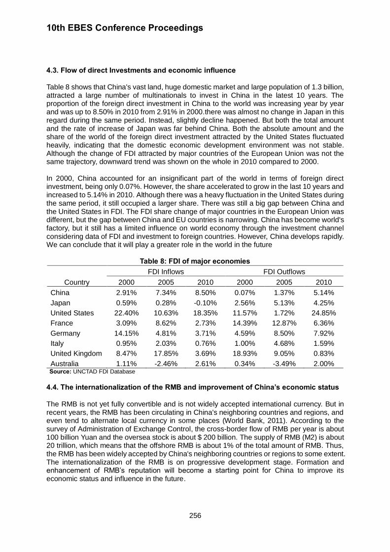
10th EBES Conference Proceedings
256
4.3. Flow of direct Investments and economic influence Table 8 shows that China's vast land, huge domestic market and large population of 1.3 billion, attracted a large number of multinationals to invest in China in the latest 10 years. The proportion of the foreign direct investment in China to the world was increasing year by year and was up to 8.50% in 2010 from 2.91% in 2000.there was almost no change in Japan in this regard during the same period. Instead, slightly decline happened. But both the total amount and the rate of increase of Japan was far behind China. Both the absolute amount and the share of the world of the foreign direct investment attracted by the United States fluctuated heavily, indicating that the domestic economic development environment was not stable. Although the change of FDI attracted by major countries of the European Union was not the same trajectory, downward trend was shown on the whole in 2010 compared to 2000. In 2000, China accounted for an insignificant part of the world in terms of foreign direct investment, being only 0.07%. However, the share accelerated to grow in the last 10 years and increased to 5.14% in 2010. Although there was a heavy fluctuation in the United States during the same period, it still occupied a larger share. There was still a big gap between China and the United States in FDI. The FDI share change of major countries in the European Union was different, but the gap between China and EU countries is narrowing. China has become world's factory, but it still has a limited influence on world economy through the investment channel considering data of FDI and investment to foreign countries. However, China develops rapidly. We can conclude that it will play a greater role in the world in the future
Table 8: FDI of major economies
Country
FDI Inflows FDI Outflows
2000 2005 2010 2000 2005 2010
China 2.91% 7.34% 8.50% 0.07% 1.37% 5.14%
Japan 0.59% 0.28% -0.10% 2.56% 5.13% 4.25%
United States 22.40% 10.63% 18.35% 11.57% 1.72% 24.85%
France 3.09% 8.62% 2.73% 14.39% 12.87% 6.36%
Germany 14.15% 4.81% 3.71% 4.59% 8.50% 7.92%
Italy 0.95% 2.03% 0.76% 1.00% 4.68% 1.59%
United Kingdom 8.47% 17.85% 3.69% 18.93% 9.05% 0.83%
Australia 1.11% -2.46% 2.61% 0.34% -3.49% 2.00% Source: UNCTAD FDI Database
4.4. The internationalization of the RMB and improvement of China’s economic status The RMB is not yet fully convertible and is not widely accepted international currency. But in recent years, the RMB has been circulating in China's neighboring countries and regions, and even tend to alternate local currency in some places (World Bank, 2011). According to the survey of Administration of Exchange Control, the cross-border flow of RMB per year is about 100 billion Yuan and the oversea stock is about $ 200 billion. The supply of RMB (M2) is about 20 trillion, which means that the offshore RMB is about 1% of the total amount of RMB. Thus, the RMB has been widely accepted by China's neighboring countries or regions to some extent. The internationalization of the RMB is on progressive development stage. Formation and enhancement of RMB’s reputation will become a starting point for China to improve its economic status and influence in the future.
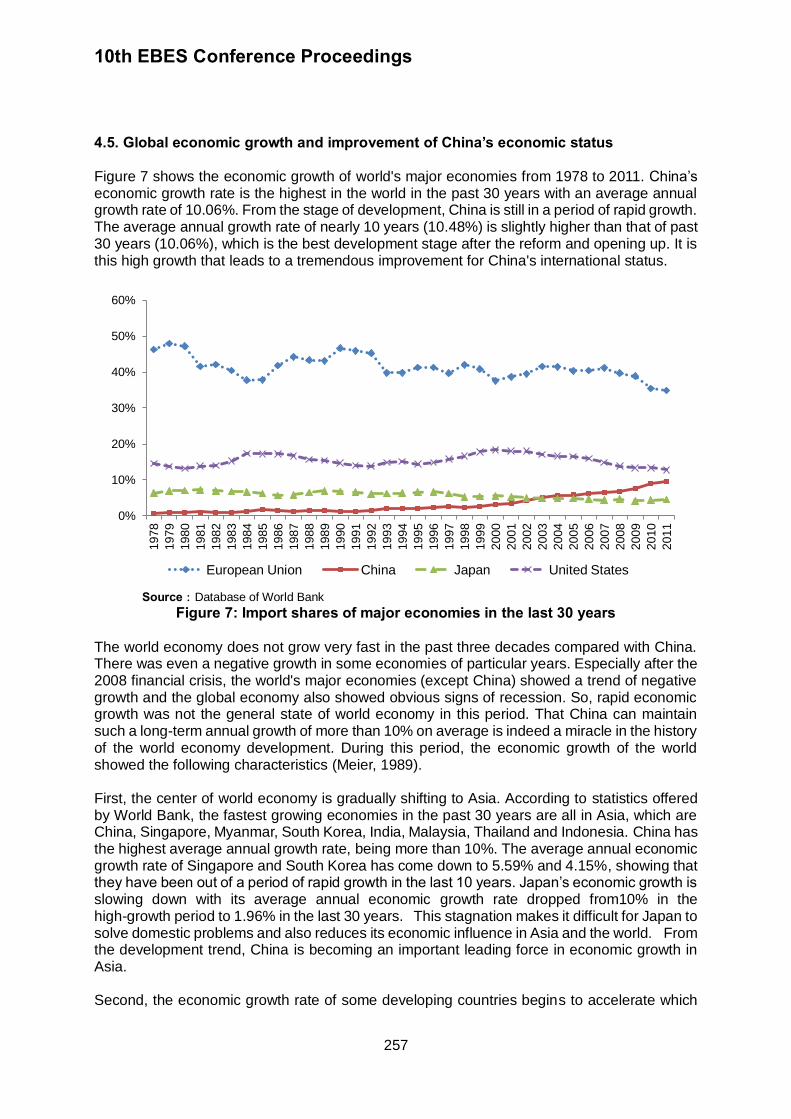
10th EBES Conference Proceedings
257
4.5. Global economic growth and improvement of China’s economic status Figure 7 shows the economic growth of world's major economies from 1978 to 2011. China’s economic growth rate is the highest in the world in the past 30 years with an average annual growth rate of 10.06%. From the stage of development, China is still in a period of rapid growth. The average annual growth rate of nearly 10 years (10.48%) is slightly higher than that of past 30 years (10.06%), which is the best development stage after the reform and opening up. It is this high growth that leads to a tremendous improvement for China's international status.
Source:Database of World Bank
Figure 7: Import shares of major economies in the last 30 years The world economy does not grow very fast in the past three decades compared with China. There was even a negative growth in some economies of particular years. Especially after the 2008 financial crisis, the world's major economies (except China) showed a trend of negative growth and the global economy also showed obvious signs of recession. So, rapid economic growth was not the general state of world economy in this period. That China can maintain such a long-term annual growth of more than 10% on average is indeed a miracle in the history of the world economy development. During this period, the economic growth of the world showed the following characteristics (Meier, 1989). First, the center of world economy is gradually shifting to Asia. According to statistics offered by World Bank, the fastest growing economies in the past 30 years are all in Asia, which are China, Singapore, Myanmar, South Korea, India, Malaysia, Thailand and Indonesia. China has the highest average annual growth rate, being more than 10%. The average annual economic growth rate of Singapore and South Korea has come down to 5.59% and 4.15%, showing that they have been out of a period of rapid growth in the last 10 years. Japan’s economic growth is slowing down with its average annual economic growth rate dropped from10% in the high-growth period to 1.96% in the last 30 years. This stagnation makes it difficult for Japan to solve domestic problems and also reduces its economic influence in Asia and the world. From the development trend, China is becoming an important leading force in economic growth in Asia. Second, the economic growth rate of some developing countries begins to accelerate which
0%
10%
20%
30%
40%
50%
60%
1978
1979
1980
1981
1982
1983
1984
1985
1986
1987
1988
1989
1990
1991
1992
1993
1994
1995
1996
1997
1998
1999
2000
2001
2002
2003
2004
2005
2006
2007
2008
2009
2010
2011
European Union China Japan United States
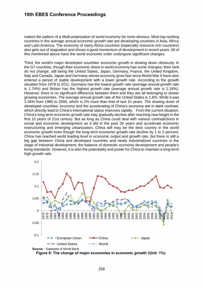
10th EBES Conference Proceedings
258
makes the pattern of a Multi-polarization of world economy be more obvious. Most top-ranking countries in the average annual economic growth rate are developing countries in Asia, Africa and Latin America. The economy of many Africa countries (especially resource-rich countries) also gets out of stagnation and shows a good momentum of development in recent years. All of this mentioned above have the world economic order undergone significant changes. Third, the world's major developed countries’ economic growth is slowing down obviously. In the G7 countries, though their economic share in world economy has some changes; their rank do not change, still being the United States, Japan, Germany, France, the United Kingdom, Italy and Canada. Japan and Germany whose economy grow fast since World War II have also entered a period of stable development with a lower growth rate. According to the growth situation from 1978 to 2011, Germany has the lowest growth rate (average annual growth rate is 1.74%) and Britain has the highest growth rate (average annual growth rate is 2.24%). However, there is no significant difference between them and they are all belonging to slower growing economies. The average annual growth rate of the United States is 1.6%. While it was 3.34% from 1980 to 2000, which is 2% more than that of last 10 years. The slowing down of developed countries’ economy and the accelerating of China’s economy are in stark contrast, which directly lead to China's international status improves rapidly. From the current situation, China's long-term economic growth rate may gradually decline after reaching new height in the first 10 years of 21st century. But as long as China could deal with various contradictions in social and economic development as it did in the past 30 years and accelerate economic restructuring and emerging urbanization, China still may be the best country in the world economic growth even though the long-term economic growth rate decline by 1 to 2 percent. China has reached world leading level in economic output and growth rate, but there is still a big gap between China and developed countries and newly industrialized countries in the stage of industrial development, the balance of domestic economy development and people's living standards. However, it is also the potentiality and power for China to maintain a long-term high growth rate.
Source:Database of World Bank
Figure 8: The change of major economies in economic growth (Unit: 1%)
-0.1
-0.05
0
0.05
0.1
0.15
0.2
1978
1979
1980
1981
1982
1983
1984
1985
1986
1987
1988
1989
1990
1991
1992
1993
1994
1995
1996
1997
1998
1999
2000
2001
2002
2003
2004
2005
2006
2007
2008
2009
2010
2011
European Union China Japan
United States World
10th EBES Conference Proceedings
259
5. CONCLUSION According to Chinese government's latest forecast, China will import 10 trillion dollars of goods from other countries with an annual average of 2 trillion dollars; invest 500 billion dollars to foreign countries. And more than 400 million people will travel outbound (See the keynote speech of Chinese President Jinping Xi at annual meeting of the 2013 Boao Forum for Asia on April 7, 2013). The rise of China will alter the balance of current growth of world economy, including trade relationship between developing countries and developed countries, international investment flows, global wealth and asset distribution, the process of industrial globalization and international currency. During this process, the altering of China’s development path, which will transfer from a extensive growth pattern to a sustainable development and expansion of domestic demand is the most motive power. While China has pulled out a series of policies which is designed to promote innovation ability of the economy in order to improve total factor productivity of economy growth. At the same time, the launch of the new urbanization plan will
greatly enhance China's domestic demand and improve economic development level. Though there is a lot of uncertainty in the process, a number of signs indicate that China’s economy will realize a smooth transition. On conclusion, China's economic development has brought development opportunities for Asia and the world and it will do better in the future. REFERENCES Atack, J. and Passell, P., 1994. A new economic view of American history: from colonial times to 1940. New York: W W Norton & Company. Faulkner, H.U., 1960. American economic history. New York: Harper & Brothers Publishers. Gunderson, G., 1976. A new economic history of America. New York: McGraw-Hill. Lim., E., Porter., I., Romer., P., and Spence., M., 2011. Medium and long term development and transformation of the Chinese economy - An international perspective. [online] Available at:<http://www.cairncrossfund.org/download/%E5%8D%81%E4%BA%8C%E4%BA%94%E9%A1%B9%E7%9B%AE%E6%8A%A5%E5%91%8A/Synthesis%20Report%20Complete%20English.pdf > [Accessed 22 January 2013]. Madison, A., 2001. The world economy: A millennial perspective. Paris: OECD. Meier, G.M., 1989. Leading issues in economic development. London: Oxford University. OECD, 2013. OECD Economic Surveys: China 2013. Paris: OECD Publishing. Wilson, C.H., 1977. The historical study of economic growth and decline in early modern history. In: E.E. Rich., M.M. Postan, and H.J. Habakkuk, eds. The Cambridge Economic History of Europe: The economic organization of early modern Europe. Vol.5. London: Cambridge University, pp.1-41. World Bank, 2011. Global development horizons 2011: Multipolarity - The new global economy. Washington, D.C.: The World Bank.
10th EBES Conference Proceedings 23 - 25 May, 2013. NIPPON HOTEL, ISTANBUL, TURKEY ISBN: 978-605-64002-1-6. WEBSITE: www.ebesweb.org
260
ANALYSIS OF RISK IN ISLAMIC AND CONVENTIONAL BANKING: SURVEY ON BAHRAIN, THE UNITED ARAB
EMIRATES AND MALAYSIA
NORAZWA AHMAD ZOLKIFLI Institute of West Asian Studies (IKRAB)
Universiti Kebangsaan Malaysia Malaysia
MOHAMAD ABDUL HAMID School of Management, Faculty of Economics and Management and Institute of
West Asian Studies (IKRAB) Universiti Kebangsaan Malaysia
Malaysia [email protected]
NOOR INAYAH YA’AKUB
School of Management, Faculty of Economics and Management and Institute of West Asian Studies (IKRAB)
Universiti Kebangsaan Malaysia Malaysia
Abstract: This paper discusses the theoretical framework of a research to investigate the
relationship of risk management with the factors that influence risk in banking. This paper highlights the relationship between credit and market risk factors that affect the risk in Islamic and conventional banking. Banking is the financial institution that faces risks in all transactions and product. All this risk has to be managed properly to ensure that the bank still can sustain. This paper incorporates a comparative analysis of Islamic and conventional bank risk management in Bahrain, United Arab Emirates and Malaysia. The data collected from financial statements of Islamic and conventional banks from these countries for a period of 10 year from 2002 to 2011. Based on the characteristics of data; i.e. combination of firm and time series from 2002 to 2011, hence this research uses panel data analysis. At the end of this paper, discussion about ensuring that Islamic and conventional banking manage the credit and market risk in risk management according with Basel I and II and also relationship of risk management with the factors that influence risk during the financial crisis. The paper will also contribute in enriching literature on risk management of Islamic banks. Keywords: Risk Management, Risk, Islamic Banking, Conventional Banking 1. INTRODUCTION
All banks around the world that practices risk management scratched due to the economic and financial crisis that invade United States when Lehman Brothers Holdings, Inc filed for bankruptcy on 15 September 2008. Failure of risk management is one of the causes of this crisis. Risk management is a continuous process that depends directly on the internal and external environment in banks. Effective risk management is a very important for the organization, including financial institutions. Financial institutions cannot operate properly
10th EBES Conference Proceedings
261
without an effective system. In fact of that, financial institutions required an effective risk management system in order to develop a strong and stable infrastructure of financial institutions. According to Errico and Sundararajan (2002) banking sector is one of the institutions of high-risk financial including the Islamic banking and conventional banking where the bank should establish a stable and effective system in risk management in order to survive in the international market.
According to Borham (2009), risk management becomes more challenging due to the unique nature of Islamic banking risk and compliance requirements to the principles. Most studies on risk management has been carried out to determine the willingness of financial institutions, including banks in which they have to comply with the rules made by Basel II related to risk management (Tufri et al. 2011). According to Khan and Ahmed (2001) also related to risk
management, explained that Islamic financial institutions are faced with a number of risks that are different from conventional financial institutions. This shows that Islamic banking has a more serious risk in conventional banking. Banking and financial institution is an unstable in the year 2007-2008 because the global financial crisis that also affected the banking and financial system (Vaaler and McNamara, 2004). The effect of these economic conditions of other countries decreases and have destroyed several banking institutions that have survived in the market to undermine public opinion against the banking system is considered stable. Islamic banking is not immune from this problem, but when compared with conventional banking, Islamic banking still can survive from this crisis with only a minimal impact. To ensure the Islamic banking can stable and avoid being exposed to risks which may affect the reputation, trust and relationships from customer that can give a very high impact (Taiquddin et al. 2012).
According Errico and Sundararajan (2002) Islamic Banking will face greater challenges in addressing and identifying the risk that each contract in the concept of the complexity of the profit and loss will exist in the product with a greater risk than the risk faced by conventional banks. Basically the risk management faced by banks in the world have to comply with the Basel I and II. With the advent of regulations under Basel 1 and Basel II credit risk and the market risk can be measured to determine the minimum capital requirements. However, many changes in the banking environment, including risk management practices, supervisory approaches and financial markets. Bank losses do not just happen to credit risk and market risk but also operational risk. The most happening risk in Islamic banking is operational risk that can give a high impact to the bank (Haron, 2005). According to Al-Tamimi and Al Mazrooei (2007) and Hassan (2009) there are three important types of risk in the banking institutions are foreign exchange risk, operational risk and credit risk. This shows that the risk incurred in banking should be given serious attention to maintain the performance of a bank. Study by Al-Tamimi and Al Mazrooei (2007) related to the comparison of local banks and foreign bank shows that the local bank is far better at managing risk. This study shows that the risk is occurring in the country itself can be controlled while the risks that occur outside of a country difficult to control. While Alam and Musukujjaman (2011) also explains the risk management techniques found that the internal classification system and risk-adjusted rate of return on capital is more important techniques in the management of the bank. This indicates that risk management is a very important thing in the banking system. This paper intends to discuss the theoretical framework of a research to investigate the relationship of risk management with the factors that influence risk in Islamic and conventional banking during the financial crisis in 2007-2008.
10th EBES Conference Proceedings
262
2. ISLAMIC BANKING SYSTEM
Islamic banking activities based on Shariah principles. Islamic bank does not allow the payment or received of interest but encourage the profit sharing in banking practices from the Islamic viewpoint. Banking term is a derivative from the word 'bank'. The word ‘bank’ comes from the Italian word 'banco' meaning strip board for the bookshelf or a table of 'bench'. The Bank is also defined as an institution that offers financial services such as currency exchange, loans and receivables bills of exchange. Islamic banking can be defined as a banking that is consistent with Islamic values and ethos. In other words, it is an institution created to provide facilities and services to the Muslims in particular bank based on Islamic law. Meaning that Islamic banking operations based on implementation principles of the Islamic. It also calls the financial institutions that have an objective to implement the principles of Islamic economics and finance in the banking arena. Bahrain is a one of the country are using Islamic and conventional banking together in a banking system. Now they become a more successful Islamic banking institution and the biggest Islamic bank in the world (Khan and Bhatti, 2008). The very popular and famous Islamic bank in Bahrain is Bahrain Islamic Bank and Faisal Islamic Bank. Both banks are main bank in Bahrain and offer an Islamic financial service to population in Bahrain. Total assets in these banks are $423m in the year 1996 where this amount is 6% from a total asset in all commercial banks in Bahrain. In fact of that total deposit for both banks are $373m that represent 5% of total deposits for 19 commercial banks in Bahrain (Central Bank of Bahrain, 2011). This amount shows that Islamic bank in Bahrain is a one of the popular banks in Bahrain.
United Arab Emirates also is the one of the country that using the dual banking system and have the oldest Islamic bank in the world such as Dubai Islamic bank that operated in 1975 and become the biggest in the world. Establishment of Dubai International Financial Centre in 2004 shows that UAE is qualified as a main financial center. In the United Arab Emirates, the financial sector accounts for 6.5% of Gross Domestic Product dominated by a strong banking industry is one of the most profitable in the world with total profits increased by 15% in 2003 alone. International Monetary Fund (2006) has accordingly to strengthen the banking sector United Arab Emirates as reflected in the ratio of 18% of its assets (the minimum is 10%), the net NPL ratio below 2%, and a wide variety of loan industries. In spite of this strength clearly shows that the potential of the banking sector in the United Arab Emirates, products and services is very important and the United Arab Emirates has introduced to the world so that they can survive in the international market.
Islamic banking in Malaysia was established on March 1, 1983 is Islamic Banking Institutions Malaysia Berhad (BIMB), which was incorporated as a Limited company in that the Companies Act 1965 (Borhan, 2005). With the establishment of the Islamic Banking shows the commitment by the government to introduce Islamic banking in Malaysia in making the institutions more involved in the banking system. To strengthen the financial system, Bank Negara Malaysia has introduced a system where commercial banks can also practice the Islamic financial by offers Islamic banking scheme where the banks can give Islamic Banking products and services to customers using bank facilities. The effectiveness of the implementation of the two banking systems can be seen through the development of Islamic banking industry in the country rapidly adopted this system. Malaysia is one of the earliest ideas pioneered Islamic banking in the world. Islamic banking has grown between 19 and 25 percent over the past 6 years and has the largest Islamic banking assets in the world among Muslim countries who practice Islamic banking which is about RM122 billion and RM6.6
10th EBES Conference Proceedings
263
billion (Annual Review, 2009). Islamic Banking System in Malaysia has become a benchmark for determining the range of specifications, progress and banking procedures throughout the world where there is 70% of global Islamic bond market and 40% of unit trusts Islam (Annual Review, 2009). Many countries are adopting Islamic Banking Malaysia as a reference in addition to get a rating of the world's leading finance companies.
From the financial crisis that surge United States, Europe and several other countries world economy and the banking sector were crippling. With the existence of Islamic banking has opened eyes around the world against the potential and success of Islamic banking system in Malaysia and West Asia. As a result, the Islamic banking system has grown rapidly in strengthening the structure and products offered to customers. According to Central Bank of Malaysia (2012) Islamic banking assets and also assets under management have reached USD750 billion and expected to reach USD1 trillion by 2020. There are more than 300 Islamic financial institutions worldwide across 75 countries and 100 Islamic banking in the world has set an annual growth rate of 26.7% of assets and the global Islamic finance industry experience 15-20% average annual growth. The growth of Islamic financial institutions in the Middle East has been a rare case where Bahrain is one of the global leaders in Islamic finance and Islamic securities become the largest producer in the world (Central Bank of Bahrain, 2011). Islamic banking also growth in particular and has been remarkable in the movement of the total assets of USD1.9 billion in 2000 to USD25.4 billion by August 2012, an increase of over 12 times. Market share of Islamic banks increased from 1.8% of total banking assets in 2000 to 13.3% in August 2012 (Central Bank of Malaysia, 2012). With this indicates that Islamic banking has been the choice of the world especially in the Middle East community now believes that the rapid development of Islamic banking has made famous throughout the world. Asian countries are one of the largest continent in the world. A total of 41 countries located in this continent with the highest number of countries, this makes Asia has the largest concentration of population. Dubai Islamic Bank located in the United Arab Emirates is the first Islamic banking in the world (Noman, 2002). The Islamic Bank system continues to expand with the establishment of the Islamic Development Bank, located in Saudi Arabia and continues to be one of the famous banks. In general, this paper will examine the risks in Islamic and conventional banking with three countries which is Bahrain, The United Arab Emirates and Malaysia.
The objective of this paper is to review the risk management relationship and the factors that can influence risk in Islamic banking and conventional banking. There are two (2) important objective of this paper are as follows :
i. To examine the relationship between credit risk and the factor that influence risk in Islamic
and conventional bank. ii. To examine the relationship between market risk and the factor that influence risk in
Islamic and conventional bank. 3. RISK IN BANKING Risk is one of the most important elements that must be faced by the banking and finance industry because each transaction always has a risk to get a profit. Risk is a very important element in the banking and finance industry, therefore the management should have a very effective and efficient in dealing with risk. These are challenges that need to be addressed very seriously by Islamic banking and conventional banking. In this paper only focused on two types of risk that are:

10th EBES Conference Proceedings
264
3.1. Credit risk
Credit risk involves the inability or failure of one party to meet its obligations as agreed upon signing the contract (Al-Saati, 2003). According to Bhatti and Misman (2010) Credit risk exists in all products that the bank offered to the customers and each bank have a different risk depend the way they manage the risk.
Studies conducted by Arunkumar and Kotreshwar (2005) show that credit risk was accounted for 70% of the total risk in the bank and 30% for market risk and operational risk. Managers of commercial banks realize that credit risk is the risk of the most common problems in the banking business (Carey and Stulz, 2005). While Khan and Ahmed (2001) explains credit risk is the most important source of banking instability is widespread and widely capital than bank insolvency. Basel Accord, the International Banking Association also noted that the largest source of risk in the banking problem is credit risk which is the risk that caused by human carelessness. According Marrison (2002), Hull (2012) and Arunkumar and Kotreshwar (2005) provide a definition of credit risk associated with the parties involved in the banking business in connection with the contract that cannot meet its contractual obligations or to repay the amount that was promised to the bank. However, Marrison (2002), was split credit risk into three parts, negligence on the loan, failure to make a payment to bondholders and trade operations.
Credit risk is the potential loss due to the failure of the counter party lenders to meet its financial obligations. The purpose of credit risk is to ensure that the structures and processes can maintain and further improve the bank's risk assessment capabilities in key areas of credit. To measure credit risk, we use the normal ratio, while it focuses on net loan charge should be eliminated one gross loans and provisions for loan losses per gross loans.
3.2. Market risk Market risk is defined as the financial risk arising from the uncertainty in the value of a portfolio of assets and liabilities. Islamic Banking is exposed to market risk when banks offer financing under the principles salam, istisna and murabaha. This will give losses to the bank
because of the changes in the market factors and policy in the economy. These changes may affect the value of financial instruments and customer flow related to give a good trade result. Price movements in different markets can give various types of market risk. Thus, market risk can be classified to equity price risk, commodity price risk, and currency risk (Khan and Ahmed, 2001). Banks will face market risk caused by the movement of market prices is not profitable and it will arise from changes in the prices of equity instruments, commodities, fixed income securities and currencies (Greuning and Iqbal, 2008). According to Haron (2005) Market risk is the potential change in value due to the volatility of movements in market rates or prices such as changes in foreign currency exchange rates, rates of return, equity prices and commodity prices. 4. FACTOR AFFECTING RISK IN BANKING
Bank is one of financial institution and it becomes same like other financial institution because the bank also faced a risk in all transactions each day. Each risk that will be found in banking can give the impact on the bank and factors that influence this risk can become a benchmark for other banks to describe the bank's position in the market. In this paper, only
10th EBES Conference Proceedings
265
four factors are discussed to identify the factors that influence the existence of risk in Islamic banking and conventional banking.
4.1. Management efficiency There are a number of studies related to management efficiency in banking (Ahmad et al. 2011; Indriani, 2008; San Ong et al. 2011; Mohi-ud-Din Sangami and Nazir, 2010; Demirovic
and Thomas, 2007). All these studies have been discussed with the management efficiency of risk management in banking.
According to San Ong et al. (2011) the achievement of local banks in Malaysia after joining in 2000 was caused by the financial crisis in Asia. From this study, the overall combined bank in Malaysia is not a significant impact on the financial performance after the merger occurred. This bank only significant achievement of return on equity, net income after expenses, earnings per share and dividends per share. Overall management efficiency had a negative relationship with financial ratios. This study, however, only be carried out on the bank merged with another bank as if made on the overall risk of commercial banks in Malaysia that occurred in the bank can be identified as a whole.
A study has been made by Mohi-ud-Din Sangami and Nazir (2010) in connection with an assessment of the financial performance of Commercial Bank in India by using the CAMEL model found that management efficiency associated with the bank's management in determining the financial position. Through this CAMEL model management efficiency has positive correlation with activity in the bank. However, this study only uses 2 banks in India which only took 5 years of data from the annual report of the bank.
From the literature, it shows that management efficiency is an important factor for the risk in Islamic and conventional banking; hence the proposed hypothesis is as follows: H1 : There is a positive relationship between credit risk and management efficiency in Islamic and conventional banking. H2 : There is a positive relationship between market risk and management efficiency in Islamic and conventional banking.
4.2. Asset management According to Tarawneh (2006) who analyze the financial performance of the banking sector to commercial banks in Oman National found that their positive relationship between asset management and financial performance. However, banks with a high amount of capital, deposits and total assets do not necessarily have a good profit performance. This is because the banks have to take into account the overall result is to improve the financial position of a bank.
Ali et al. (2011) also study on indicators of conventional banking profit by the private sector
and the government in the country of Pakistan in the year 2006-2009. This study found that the efficiency of asset management and stable economic growth had a positive relationship with profitability. However, this study only used return on assets and return on equity for the most significant relationship to profit.
Finally it is found that asset management is particularly important in managing risk in banking. Hence the proposed hypothesis is as follows:
10th EBES Conference Proceedings
266
H3 : There is a positive relationship between credit risk and asset management in Islamic and conventional banking.
H4 : There is a positive relationship between market risk and asset management in Islamic and conventional banking.
4.3. Operation efficiency According to Alkhatib (2012), greatly affects the operational efficiency of the financial performance of commercial banks in Palestine. Studies show that efficient operations have a negative relationship with financial performance in which all models are used in view of operational efficiency has a negative relationship with financial performance. This shows the efficiency of the operation does not affect the financial performance of a bank. According Ali et al. (2011) also operational efficiency has a negative relationship with return on assets and return on equity. This suggests that the efficiency of operations not directly related to financial performance. While Tarawneh (2006) also found that operational efficiency has a positive relationship with financial performance in which the study relates to the five commercial banks with 260 branches of the bank throughout Oman where operational efficiency have a very strong relationship with financial performance. According to San Ong et al. (2011) the achievement of local banks in Malaysia after joining in
2000 was caused by the financial crisis in Asia. From this study, the overall combined bank in Malaysia is not a significant impact on the financial performance after the merger occurred. This bank only significant achievement of return on equity, expenses to earnings, earnings per share and dividends per share. Overall efficiency has a negative relationship with financial ratios. However, this study only focused on the approach Data Envelopment analysis (DEA) is used to measure improvement in bank efficiency after the merger. Finally, from literature, it is suggested that operational efficiency is one of the important factors; hence, the proposed hypothesis is as follows: H5 : There is a negative relationship between credit risk and operational efficiency in Islamic and conventional banking. H6 : There is a negative relationship between market risk and operational efficiency in Islamic and conventional banking.
4.4. Profitability efficiency Six Islamic Banking and Conventional Banking 15 were selected for the study conducted by Samad (2004) found that there is no difference between Islamic banking and conventional banking in Bahrain. This shows that the profitability efficiency are not significantly different between the two systems that used in the bank.
According to San Ong et al. (2011) to increase the return on assets and return on equity,
enables banks to make a profit after the bank merger among the others bank. While Tarawneh (2006) also found that banks with higher capital, deposits and total assets is not necessarily have a high profit. Ali et al. (2011) also stated that the internal factors such as the
size of the bank, profitability, operating efficiency, capital, credit risk, portfolio composition and asset management influence the profitability bank. These factors that have been mentioned have a positive relationship with bank profitability.
10th EBES Conference Proceedings
267
Finally, profitability is important factors to ensure that risk in Islamic and conventional banking can manage properly, hence, the proposed hypothesis is as follows: H7 : There is a positive relationship between credit risk and profitability efficiency in Islamic and conventional banking. H8 : There is a positive relationship between market risk and profitability efficiency in Islamic and conventional banking. 5. DISCUSSION Risk is part of the financial issue. Financial institutions can survive and prosper depends on its effectiveness in managing risk. Akkizidis and Khandelwal (2008) categorize the risks to financial risk, business risk and operational risk. Due to a movement in financial variables and there is the possibility of losses in the market, financial risk can occur. Business risks arising from the nature of the business firm related to the factors that influence product market. While operational risk arises from the failure of processes, systems and parties involved in the institution or things that are out of institutions such as the things that can cause a disaster. The existences of risk due to numerous factors are usually deal with credit and market risk. This paper relates to the risks inherent in Islamic and conventional banking that could affect the factor in banking risk. These two types of risk will be reviewed and the focus of the investigation to be carried out. Many studies have been conducted on the types of risk such as Ahmad et al. (2011) who discussed the three types of risk such as credit,
liquidity and operational risks. But there is still no study had discussed all this risk in a complete study. This is because with a discussion of the two types of risk, will strengthen an opinion on the risks in Islamic banking and conventional banking as well as in relation to the existence of risk factors affecting the banking industry.
This paper will make a comparative analysis of three countries, such as, Bahrain, Malaysia and the United Arab Emirates. Countries selected for this study on the basis that the three countries have a banking system similar to each other in which Malaysia, Bahrain and the United Arab Emirates using the Islamic banking system and in the same time also using conventional banking system (Akkizidis and Khandelwal, 2008). Malaysia's position as an Islamic banking operations in the world's largest single consumer banking in a very good perspective on Islamic banking industry. This makes the famous Malaysian Islamic banking system that is trusted by the community. While the United Arab Emirates was chosen for Abu Dhabi Investment Authority, where the firm is the largest firm in the world related to sovereign wealth funds. Bahrain also is as one of the most actively promoting Islamic finance across the country and make a country can survive in the Islamic banking industry despite the global financial crisis was hit. A comparative analysis is made between the three countries involved in this study so that they could strengthen the Islamic banking system in each country and can contribute to the other country are using Islamic Banking practice.
The main thing that distinguishes Islamic banking with conventional banking is in operation where Islamic banking operates without involving the element of interest. This is because Islam prevents Muslims from giving or receiving or take usury, in addition to its objectives is to meet the needs of Muslims in the banking business. This study also makes a comparison between Islamic banking and conventional banking for the three countries involved in terms of the factors that influence risk. With this comparison, this paper will identify the factors that can influence the risk for each Islamic banking and conventional banking in the three countries.
10th EBES Conference Proceedings
268
6. CONCLUSION Islamic banking has also begun to emphasize risk management in their banking activities as has been done by conventional banks. Risk management practices are also becoming more important as Islamic banking should also be compliant with the Basel I and Basel II, which took effect in 2006. Risks faced by each bank are different from each other. The risks involved include credit, market, liquidity, operational and profit-sharing. In theory if adoption of Islamic values is quite high among users of Islamic banking services, appropriate risk involved is low compared with the risks faced by conventional banking. In conclusion, the conceptual and empirical literature has explained the relationship between risk and factor that influence risk in Islamic and conventional banking. Further researches are needed to prove empirically the hypothesis suggested and the factor that influence risk in banking can be determined. REFERENCES Ahmed, N., Akhtar, M.F., and Usman, M., 2011. Risk management practices and Islamic banks: An empirical investigation from Pakistan. Interdisciplinary Journal of Research in Business, 1(6), pp.50-57.
Akkizidis, I.S. and Khandelwal, S.K., 2008. Financial risk management for Islamic banking and finance. Great Britian: Palgrave Macmillan.
Alam, M.Z. and Musukujjaman, M., 2011. Risk management practices : A critical diagnosis of some selected commercial banks in Bangladesh. Journal of Business and Technology (Dhaka), 6(1), pp.15-35. Ali, K., Akhtar, M.F., and Ahmed, H.Z., 2011. Bank-specific and macroeconomic indicators of profitability-empirical evidence from the commercial banks of Pakistan. International Journal of Business and Social Science, 2(6), pp.235-242. Alkhatib, A. and Harsheh, M., 2012. Financial performance of palestinian commercial banks. International Journal of Business and Social Science, 3(3), pp.175-184. Al-Saati, A.R., 2003. The permissible gharar (risk) in classical Islamic Jurisprudence. Islamic Economics, 16(2), pp.3-19
Al-Tamimi, H.A.H. and Al Mazrooei, F.M., 2007. Bank's risk management : A comparison study of UAE Nation and Foreign Banks. Journal of Risk Finance, 8(4), pp.394-409.
Annual Review, 2009. Malaysia's economic outlook 2009-2020. Kuala Lumpur: RAM
Holdings Berhad. Arunkumar, R. and Kotreshwar, G., 2005. Risk management in commercial banks (A case study of public and private sector banks). [Online] Available at: <http://papers.ssrn.com/sol3/papers.cfm?abstract_id=877812> (Accessed 18 November 2012).
Bhatti, I. and Misman, F., 2010. Risk exposure in Islamic Banks: A case study of Bank Islam Malaysia Berhad (BIMB). [Online] Available at:
<http://papers.ssrn.com/sol3/papers.cfm?abstract_id=1632849> (Accessed 21 January 2013).
10th EBES Conference Proceedings
269
Borham, A.J., 2009. Banking industries and Islamic finance. Kuantan, Pahang: Universiti Malaysia Pahang. Borhan, J.T., 2005. Implementation of Syariah principle in Islamic banking in Malaysia. Theory and Application of Contemporary Islamic Economics System in Malaysia. Kuala
Lumpur: Utusan Publication and Distributors. Carey, M. and Stulz, R.M., 2005. The risks of financial institutions (No. W11442). National Bureau of Economic Research.
Central Bank of Bahrain, 2011. Annual report 2012. Central Bank of Malaysia, 2012. Annual report 2011. Demirovic, A. and Thomas, D.C., 2007. The relevance of accounting data in the measurement of credit risk. The European Journal of Finance, 13(3), pp.253-268. Errico, L. and Sundararajan, V., 2002. Islamic financial institutions and products in the global financial system : Keys issues in risk management and challenges ahead (Vol. 2). International Monetary Fund.
Greuning, H.V. and Iqbal, Z., 2008. Risk analysis for islamic banks. Washington, D.C: The
World Bank. Haron, S., 2005. Financial system and Islamic banking. Kuala Lumpur: Kuala Lumpur
Business School Sdn Bhd. Hassan, A., 2009. Risk management practices of Islamic banks of Brunei Darussalam. The Journal of Risk Finance, 10(1), pp.23-37.
Hull, J., 2012. Risk management and financial institutions. New Jersey: Wiley.
Indriani, V., 2008. The relationship between Islamic financing with risks and performance of commercial banks in Indonesia. Doctoral Dissertation: University of Indonesia.
International Monetary Fund, 2006. Kingdom of Bahrain: Financial system stability assessment, including reports on the observance of standard and codes on the following topics, banking and insurance supervision, securities regulation, and anti-money laundering and combating the financing . Washington: IMF.
Khan, M.M. and Bhatti, M.I., 2008. Development in Islamic banking: A financial risk-allocation approach. The Journal of Risk Finance, 9(1), pp.40-51.
Khan, T. and Ahmed, H., 2001. Risk management : An analysis of issues in islamic financial industry. Islamic Development Bank: Islamic Research and Training Institute.
Marrison, C., 2002. The fundamentals of risk measurement. New York: McGraw Hill.
Mohi-ud-Din Sangami, D. and Nazir, T., 2010. Analyzing financial performance of commercial banks in India: Application of CAMEL model. Journal of Commercial Social Science, 4, pp.40-55.
10th EBES Conference Proceedings
270
Noman, A.M., 2002. Imperatives of financial innovation for Islamic banks. International Journal of Islamic Financial Services, 4(3), pp.1-10
Samad, A., 2004. Performance of interest-free Islamic banks Vis-A-Vis interest based convenstional banks of Bahrain. Journal of Economics and Management, 12(2), pp.1-15.
San Ong, T., Teo, C.L., and Teh, B.H., 2011. Analysis on financial performance and efficiency changes of Malaysian commercial banks after mergers and acquisitions. International Journal of Business and Management Tomorrow, 1(2), pp.1-16.
Taiquddin, M., Borhan, J.T., and Azam, A., 2012. Challenges facing Islamic banking relevance financial instability. Seventh Malaysian National Economic Conference (PERKEM VII). Ipoh Perak, Malaysia 4-6 June 2012. Malaysia: University Kebangsaan Malaysia. Tarawneh, M., 2006. A comparison of financial performance in the banking sector: Some evidence from Omani commercial banks. International Research Journal of Finance and Economics, 3, pp.101-112.
Tufri, F.H., Rahman, R.A., and Omar, N. 2011. Empirical evidence on the risk management tools practised in Islamic and conventional banks. Qualitative Research in Financial Market, 3(2), pp.86-104.
Vaaler, P.M. and McNamara, G., 2004. Crisis and competition in expert organization decision making. Credit-rating agencies and their response to turbulence in emerging market. Organization Science, 15(6), pp.687-703.
10th EBES Conference Proceedings 23 - 25 May, 2013. NIPPON HOTEL, ISTANBUL, TURKEY ISBN: 978-605-64002-1-6. WEBSITE: www.ebesweb.org
271
GENDER AND HOUSEHOLD EDUCATION EXPENDITURE IN TURKEY
Z. BILGEN SUSANLI
Department of Economics Işık University
Turkey [email protected]
Abstract: This paper investigates how the share of education expenditure in the household
budget varies across Turkish households with different gender-age composition of children. Using household level data from Household Budget Surveys over the period 2004 – 2008, I find no evidence for a pro-male bias. Results suggest that a pro-female bias at the secondary school level emerged in 2006 which is in line with declining gender gaps in enrolment at the secondary school level. Findings in both urban and rural areas suggest that Turkish households do not favor boys in the allocation of education expenditures. To the contrary, in 2006 girls of secondary school age group receive more educational resources than boys of the same age group. This may be explained by the effect of both education and textbook assistance campaigns. Further research is needed to make other labor market oriented explanations. Keywords: Education Expenditure, Household, Gender, Turkey
1. INTRODUCTION
It is well known that girls have inferior education outcomes than boys in the developing world (World Bank, 2011). Gender gaps in education outcomes may reflect discrimination at the labor market in the form of lower returns to schooling for females as well as differential access to household resources. The focus of this paper is the latter which, in turn, may be resulting from gender bias in the allocation of resources depending on the gender of the recipient. Empirical evidence supports the existence of pro-male bias in education expenditure at the household level in many developing countries (Burgess and Zhuang, 2000; Kingdon, 2005; Aslam and Kingdon, 2008; Azam and Kingdon, 2011; Zimmermann, 2012; Masterson, 2012) except for the Srilankan case where a pro-female bias is detected (Himaz, 2010). Turkey still has gender gaps in secondary education. Gender gap virtually disappeared at the primary school level, most probably due to the 8-Year Basic Education Program initiated in 1997. In addition, between 2003 and 2006, the Ministry of National Education, together with UNICEF, implemented an education campaign, Haydi Kızlar Okula! to encourage the schooling of girls in areas with the lowest enrolment rates. This campaign has largely been successful at the primary education level, reflected in the recent increase in female enrolment rates.1 In 2008 female and male primary enrolment rates reached 94 and 97 percent, respectively (Figure 1). However, the same cannot be said for secondary education (Figure 2). Despite the fall in gender gap at secondary school level from 17 percent in 1994 to 7 percent in 2008, Turkey is still behind many developing countries including India, Indonesia, Morocco and Tunisia in terms of the ratio of female-to-male secondary school
1
During the campaign period, of the 273,447 school-going age female children that were identified as out- of-school, 81 percent has been enrolled in school. (http://haydikizlarokula.meb.gov.tr/). In 2005 a similar campaign was started with the leadership of media and support from the business world. This campaign also aimed to support the schooling of girls that were out-of-school due to financial and family reasons.
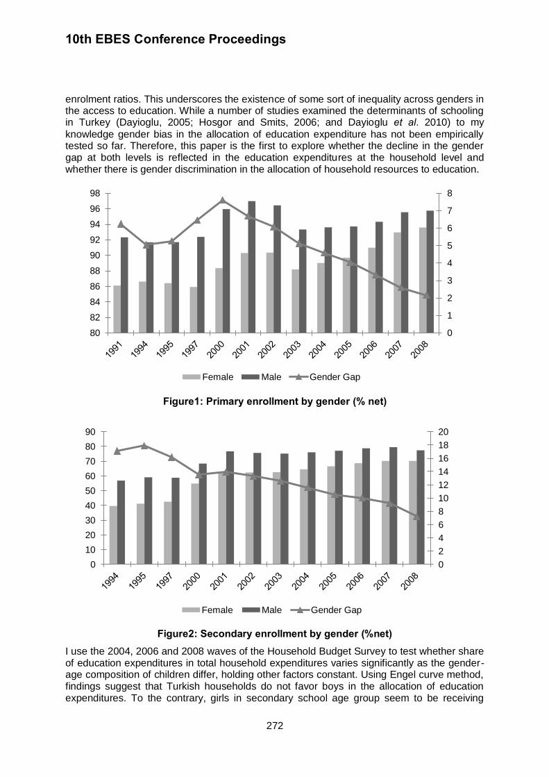
10th EBES Conference Proceedings
272
enrolment ratios. This underscores the existence of some sort of inequality across genders in the access to education. While a number of studies examined the determinants of schooling in Turkey (Dayioglu, 2005; Hosgor and Smits, 2006; and Dayioglu et al. 2010) to my
knowledge gender bias in the allocation of education expenditure has not been empirically tested so far. Therefore, this paper is the first to explore whether the decline in the gender gap at both levels is reflected in the education expenditures at the household level and whether there is gender discrimination in the allocation of household resources to education.
Figure1: Primary enrollment by gender (% net)
Figure2: Secondary enrollment by gender (%net) I use the 2004, 2006 and 2008 waves of the Household Budget Survey to test whether share of education expenditures in total household expenditures varies significantly as the gender-age composition of children differ, holding other factors constant. Using Engel curve method, findings suggest that Turkish households do not favor boys in the allocation of education expenditures. To the contrary, girls in secondary school age group seem to be receiving
0
1
2
3
4
5
6
7
8
80
82
84
86
88
90
92
94
96
98
Female Male Gender Gap
0
2
4
6
8
10
12
14
16
18
20
0
10
20
30
40
50
60
70
80
90
Female Male Gender Gap
10th EBES Conference Proceedings
273
more educational resources than boys. These findings accord well with declining gender gaps in school enrolment. The rest of the paper is structured as follows. Section 2 describes the dataset used. Section 3 explains the empirical methodology. Empirical findings are discussed in section 4 and section 5 concludes. 2. DATA I explore data from Household Budget Survey for 2004, 2006 and 2008, collected by Turkish Statistical Institute (TUIK). The household budget surveys are cross-sections in which 720 households are surveyed each month amounting to about 8,500 households from urban and rural areas each year. The surveys include rich information about household expenditures on several consumption items such as food, housing, transportation, health, restaurants and entertainment as well as education. Of particular interest is the data on househo lds’ expenditure on education services in the reference month. The expenditure on education is separately available for preschool, primary school, secondary school and university at the household level. This variable captures any expenditure on education including installment payments of private school tuition, if any. Spending on books and education materials are included in the culture and entertainment expenditures group and are also available separately in the data. The main variable of interest in this study is the share of total education expenditures at the primary and secondary level as well as spending on books and materials in the total household expenditures in the reference month reported by the households. It is important to mention important policy changes that were adopted by the Ministry of Education in Turkey during the period of this study. The Ministry of Education initiated textbooks assistance for students which included free provision of textbooks at the beginning of each semester. This policy came into effect in 2004 and 2006 at the primary school and secondary school level, respectively. On the one hand, such a policy is expected to increase enrolment by lowering the cost of schooling. One the other hand, it would suppress variation of education expenditures and hence mute any underlying gender bias, if any. In addition, the duration of secondary school education, which follows 8-years of mandatory school education, was extended from 3 to 4 years in 2005-2006. While this may not directly influence within household allocation of education expenditure, it may affect enrolment decisions especially when the opportunity cost of going to school is considered in rural areas. Table 1 presents summary statistics of the variables used in the sample. The share of education expenditure in total household expenditure is around 1.7 percent. This rather small share of education expenditure is expected considering the availability and prevalence of public schools that are largely free as well as the infrequent nature of education expenditure.
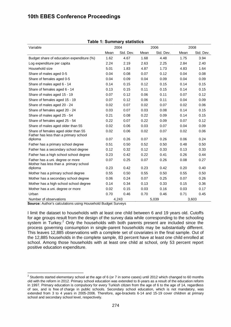
10th EBES Conference Proceedings
274
Table 1: Summary statistics
Variable 2004 2006 2008
Mean Std. Dev. Mean Std. Dev. Mean Std. Dev.
Budget share of education expenditure (%) 1.62 4.67 1.68 4.48 1.75 3.94
Log expenditure per capita 2.24 2.19 2.63 2.25 2.84 2.40
Household size 5.01 1.83 4.87 1.73 4.83 1.64
Share of males aged 0-5 0.04 0.08 0.07 0.12 0.04 0.08
Share of females aged 0-5 0.04 0.09 0.04 0.09 0.04 0.09
Share of males aged 6 - 14 0.14 0.15 0.12 0.15 0.14 0.15
Share of females aged 6 - 14 0.13 0.15 0.11 0.15 0.14 0.15
Share of males aged 15 - 19 0.07 0.12 0.06 0.11 0.07 0.12
Share of females aged 15 - 19 0.07 0.12 0.06 0.11 0.04 0.09
Share of males aged 20 - 24 0.02 0.07 0.02 0.07 0.02 0.06
Share of females aged 20 - 24 0.03 0.07 0.03 0.08 0.14 0.15
Share of males aged 25 - 54 0.21 0.08 0.22 0.09 0.14 0.15
Share of females aged 25 - 54 0.22 0.07 0.22 0.09 0.07 0.12
Share of males aged older than 55 0.02 0.06 0.03 0.07 0.04 0.09
Share of females aged older than 55 0.02 0.06 0.02 0.07 0.02 0.06 Father has less than a primary school diploma 0.07 0.26 0.07 0.26 0.06 0.24
Father has a primary school degree 0.51 0.50 0.52 0.50 0.48 0.50
Father has a secondary school degree 0.12 0.32 0.12 0.33 0.13 0.33
Father has a high school school degree 0.23 0.42 0.22 0.41 0.26 0.44
Father has a uni. degree or more 0.07 0.25 0.07 0.26 0.08 0.27 Mother has less than a primary school diploma 0.23 0.42 0.23 0.42 0.20 0.40
Mother has a primary school degree 0.55 0.50 0.55 0.50 0.55 0.50
Mother has a secondary school degree 0.06 0.24 0.07 0.25 0.07 0.26
Mother has a high school school degree 0.14 0.34 0.13 0.33 0.15 0.36
Mother has a uni. degree or more 0.02 0.15 0.03 0.16 0.03 0.17
Urban 0.70 0.46 0.70 0.46 0.71 0.45
Number of observations 4,243 5,039 3,603
Source: Author's calculations using Household Budget Surveys I limit the dataset to households with at least one child between 6 and 19 years old. Cutoffs for age groups result from the design of the survey data while corresponding to the schooling system in Turkey.2 Only the households with both parents present are included since the process governing consumption in single-parent households may be substantially different. This leaves 12,885 observations with a complete set of covariates in the final sample. Out of the 12,885 households in the complete sample, 83 percent have at least one child enrolled at school. Among those households with at least one child at school, only 53 percent report positive education expenditure. 2 Students started elementary school at the age of 6 (or 7 in some cases) until 2012 which changed to 60 months
old with the reform in 2012. Primary school education was extended to 8-years as a result of the education reform in 1997. Primary education is compulsory for every Turkish citizen from the age of 6 to the age of 14, regardless of sex, and is free of charge in public schools. Secondary school education, which is not mandatory, was extended from 3 to 4 years in 2005-2006. Therefore, age-brackets 6-14 and 15-19 cover children at primary school and secondary school level, respectively.

10th EBES Conference Proceedings
275
3. EMPIRICAL STRATEGY If expenditure data on each child were available, a direct comparison across male and female children would be possible. However, using household level data, intra-household differences in education expenditures can only be estimated indirectly. I examine whether the budget share of education expenditure differs significantly across households with different compositions of age and gender. Following Aslam and Kingdon (2008) and Himaz (2010), I estimate the following the Working Lesser specification for demand analysis:
ii
1Jj
1j i
ij
ijii
ii εδz
n
nθnγlnn
xβlnαw
(1)
where iw is the budget share of education of the ith household, ix is total household
expenditure, in is the size of the household,
i
i
nx
ln is the natural log of per capita total
expenditure, ijn is the number of household members that belong to age-gender class j, zi
captures other household characteristics such as mother’s and father’s education levels and
the place of residence, and i is the error term. The main coefficient of interest is ij which
can be calculated separately for males and females. Gender bias can be tested by an F-test
of the null hypothesis, gfgm , where m denotes males and f denotes females and
g={1,2,…G} refers to a specific age group. Since these shares add up to unity, one of them
has to be excluded from the model. I allow for 6 age groups for male and females: 0-5, 6-14, 15-19, 20-24, 25-54 and 55 and above. I omit the share of females in the 25-54 age group from the analysis. Age groups 6-14 and 15-19 are important since they correspond to children at the primary school and secondary school level, respectively
The coefficient, , is also important in that it determines whether education is a luxury or
necessity depending on the sign. A positive sign would imply a luxury whereas a negative one would imply a necessity. 4. RESULTS
I estimate the Engel curves by estimating equation (1) using ordinary least squares. F-tests for the equality of coefficients on share of males and females in the same age group and corresponding p-values are presented at the bottom of each column. Column (1) in table 2
displays the results using the pooled sample across all years controlling for year dummies. The coefficient of household size is positive and significant which may reflect economies of scale but also the fact that larger households may have more children of school-going age and hence they allocate a greater share of their budgets to education. The coefficients on shares of both males and females aged 15-19 are positive and significant. The p-value of the F-test that the coefficient on share of females aged 15-19 equals the coefficient on share of
males aged 15-19 is 0.02, which implies that budget share of education increases more when an extra girl aged 15-19 is added to the household than when an extra boy aged 15-19 is added. The coefficients of shares of males and females in the primary-school age group are both positive but not statistically significant. Coefficients of the parental education are also positive and statistically significant for high school and university level or more for mother and fathers, respectively. This indicates a higher demand for education expenditure in households with more educated parents.

10th EBES Conference Proceedings
276
The positive and significant coefficient of the log of per capita expenditure indicates that education is treated as a luxury. To address the potential endogeneity of household expenditure per capita an instrumental variables model is also estimated. About 70 percent of households in the sample report a positive amount of unearned income in the form of interest income and rents. I use unearned income and its square as instruments. Results are shown in column (2).3 While the magnitudes of coefficients change, the coefficients on share of males and females aged 6-14 are now significant. While the coefficient on share of females aged 6-14 is greater than that of males in the same age group, F-test implies that there is no gender bias favoring girls over
boys. Considering that the education campaigns to increase the enrolment of girls were initiated in 2003 and 2005 and textbook assistance programs were launched in 2004 and 2005, estimating the model separately for each year may give useful insights. Columns (3) – (5) show the results for each year separately. Some interesting features emerge. First, no gender bias is detected for children in 6-14 age group which may reflect the impact of the policy changes during the period. Second, F-tests do not suggest a gender bias in favor of females, except in 2006. In 2006, for example, if a child between ages 15-19, had been a girl rather than a boy in the same household, 3.2 percent more funds would have been spent on her education, controlling for all other factors. In addition, the coefficient of the log expenditure per capita is positive and significant in all years implying that education is a luxury good. The increase in the magnitude of the coefficient over the period may suggest that education has become treated as more of a luxury good over time. This may be an artifact of textbooks assistance programs which may substantially help parents with lowering education expenditures. The coefficient of household size is also positive and significant starting with 2006. This may indicate that for any given level of per capita expenditure larger households benefit from economies of scale that come from shared goods. In the context of education expenditures, this may be explained by children in larger households sharing their school supplies and uniforms with their siblings. However, one can also argue that household size may be endogenous such that parents with a higher taste for education may choose smaller households and also a higher budget share of education.4 Surprisingly, parental education variables are not significant in any of the years except 2006 where the coefficient on father has a primary school degree is negative and significant. Since enrolment and expenditure decisions are expected to be different for urban and rural areas, looking at these two areas separately may uncover underlying patterns. Table 3 presents the coefficients of interest from separate regressions that estimate equation (1) using rural and urban subsamples for each year. Some interesting features emerge. First, more resources are allocated to education for both genders in both age-groups (relative to the base category) in urban areas than in rural areas. Second, female children in age group 15-19 receive more educational resources than males in the same age group, relative to the base category, in all subsamples and all years except the 2004 rural subsample. Finally, a
3 An F-test on the joint significance of the instruments implies that the instruments are jointly significant at 5
percent level which confirms the relevance of the instruments. An overidentification test confirms that the instruments are valid. The Durbin-Wu-Haussman test fails to reject the endogeneity of log expenditure per capita using a regression test. Hence, in the remainder of the paper, results from the instrumental variables estimation will be reported. 4 Unfortunately, we do not have data on households over time to address the endogeneity of household size by
using a fixed effects method.
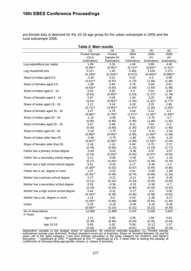
10th EBES Conference Proceedings
277
pro-female bias is detected for the 15-19 age group for the urban subsample in 2006 and the rural subsample 2008.
Table 2: Main results (1) (2) (3) (4) (5)
Pooled Sample (OLS
Estimation)
Pooled Sample (IV Estimation)
2004 (IV
Estimation)
2006 (IV
Estimation)
2008 (IV
Estimation)
Log expenditure per capita 1.09 3.32 1.84 3.68 4.48 (0.09)** (0.55)** (0.71)** (0.84)** (1.51)** Log Household size 0.317 1.45 0.363 1.616 2.372 (0.140)* (0.319)** (0.572) (0.440)** (0.886)** Share of males aged 0-5 -2.65 0.51 0.22 0.3 0.98 (0.61)** (0.97) (1.73) (1.56) (1.94) Share of females aged 0-5 -1.89 0.84 0.79 0.68 0.91 (0.63)** (0.93) (1.69) (1.44) (1.98) Share of males aged 6 - 14 0.55 2.82 2.3 2.54 3.48 (0.61) (0.85)** (1.63) (1.27)* (1.78) Share of females aged 6 - 14 0.87 3.08 1.94 3.25 3.88 (0.61) (0.85)** (1.55) (1.32)* (1.77)* Share of males aged 15 - 19 2.12 3.34 4.28 2.25 2.96 (0.71)** (0.80)** (1.67)* (1.20) (1.50)* Share of females aged 15 - 19 3.47 4.75 4.06 5.42 4.3 (0.68)** (0.78)** (1.57)** (1.18)** (1.49)** Share of males aged 20 - 24 -1.14 -0.96 0.61 -2.76 -0.7 (0.90) (0.95) (1.95) (1.48) (1.82) Share of females aged 20 - 24 0.57 0.98 0.41 1.62 0.2 (0.56) (0.60) (1.35) (0.81)* (1.66) Share of males aged 25 - 54 -2.33 -2.75 -1.53 -4.13 -2.53 (0.88)** (0.95)** (1.80) (1.55)** (1.98) Share of males older than 55 -2.46 -2.75 -1.85 -4.39 -1.15 (0.92)** (0.98)** (1.99) (1.53)** (2.04) Share of females older than 55 0.18 1.16 0.84 0.79 2.72 (0.76) (0.84) (1.76) (1.23) (1.71) Father has a primary school degree -0.09 -0.62 -0.38 -0.57 -0.97 (0.13) (0.20)** (0.35) (0.27)* (0.52) Father has a secondary school degree 0.11 -0.65 -0.45 -0.4 -1.16 (0.17) (0.26)* (0.47) (0.35) (0.70) Father has a high school school degree 0.51 -0.54 0.17 -0.46 -1.4 (0.18)** (0.32) (0.57) (0.44) (0.85) Father has a uni. degree or more 1.07 -0.51 0.91 -0.65 -1.88 (0.26)** (0.45) (0.74) (0.66) (1.20) Mother has a primary school degree 0.17 -0.31 -0.11 -0.43 -0.48 (0.11) (0.15)* (0.23) (0.25) (0.40) Mother has a secondary school degree 0.26 -0.36 -0.15 -0.38 -0.7 (0.19) (0.24) (0.40) (0.42) (0.52) Mother has a high school school degree 0.64 -0.41 -0.17 -0.4 -0.82 (0.18)** (0.30) (0.45) (0.48) (0.81) Mother has a uni. degree or more 1.12 -0.6 0.03 -1.49 -0.27 (0.43)** (0.60) (0.98) (0.91) (1.40) Urban 0.28 -0.18 -0.04 -0.18 -0.36
(0.08)** (0.14) (0.21) (0.21) (0.36)
No of observations 12,885 12,885 4,243 5,039 3,603 F-Tests:
Age 6-14: 1.11 0.69 0.39 1.69 0.61 (0.30) (0.40) (0.53) (0.20) (0.43)
Age 15-19: 5.65 5.82 0.06 10.12 1.37 (0.02) (0.02) (0.81) (0.00) (0.24)
Dependent variable is the budget share of education. All columns estimate equation (1). Pooled sample estimations include year dummies. Robust standard errors are in brackets. Share of females between 25 and 54 years old is the base category. Less than primary education is the base category for mother's and father's education. * significant at 10%; ** significant at 5%; *** significant at 1%. F-tests refer to testing the equality of coefficients of corresponding age-gender shares, p- values in brackets.
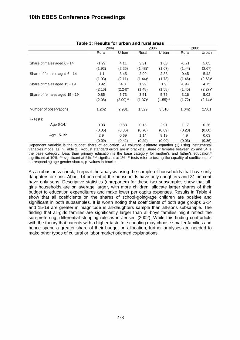
10th EBES Conference Proceedings
278
Table 3: Results for urban and rural areas 2004 2006 2008
Rural Urban Rural Urban Rural Urban
Share of males aged 6 - 14 -1.29 4.11 3.31 1.68 -0.21 5.05
(1.92) (2.26) (1.48)* (1.67) (1.44) (2.67)
Share of females aged 6 - 14 -1.1 3.45 2.99 2.88 0.45 5.42
(1.93) (2.11) (1.44)* (1.78) (1.46) (2.68)*
Share of males aged 15 - 19 3.92 4.8 1.99 1.9 -0.47 4.75
(2.16) (2.24)* (1.48) (1.58) (1.45) (2.27)*
Share of females aged 15 - 19 0.85 5.73 3.51 5.76 3.16 5.02
(2.08) (2.09)** (1.37)* (1.55)** (1.72) (2.14)*
Number of observations 1,262 2,981 1,529 3,510 1,042 2,561
F-Tests:
Age 6-14: 0.03 0.83 0.15 2.91 1.17 0.26
(0.85) (0.36) (0.70) (0.09) (0.28) (0.60)
Age 15-19: 2.9 0.69 1.14 9.19 4.9 0.03
(0.09) (0.42) (0.29) (0.00) (0.03) (0.86)
Dependent variable is the budget share of education. All columns estimate equation (1) using instrumental variables model as in Table 2. Robust standard errors are in brackets. Share of females between 25 and 54 is the base category. Less than primary education is the base category for mother's and father's education.* significant at 10%; ** significant at 5%; *** significant at 1%. F-tests refer to testing the equality of coefficients of corresponding age-gender shares, p- values in brackets.
As a robustness check, I repeat the analysis using the sample of households that have only daughters or sons. About 14 percent of the households have only daughters and 31 percent have only sons. Descriptive statistics (unreported) for these two subsamples show that all-girls households are on average larger, with more children, allocate larger shares of their budget to education expenditures and make lower per capita expenses. Results in Table 4 show that all coefficients on the shares of school-going-age children are positive and significant in both subsamples. It is worth noting that coefficients of both age groups 6-14 and 15-19 are greater in magnitude in all-daughters sample than all-sons subsample. The finding that all-girls families are significantly larger than all-boys families might reflect the son-preferring, differential stopping rule as in Jensen (2002). While this finding contradicts with the theory that parents with a higher taste for schooling may choose smaller families and hence spend a greater share of their budget on allocation, further analyses are needed to make other types of cultural or labor market oriented explanations.

10th EBES Conference Proceedings
279
Table 4: Robustness checks All-girls households All-boys households
Log expenditure per capita 6.59 3.43
(2.26)*** (0.76)***
Log Household size 2.17 1.65
(1.20)* (0.44)***
Share of children aged 0 -5 5.74 1.00
(3.48)* (1.38)
Share of children aged 6 - 14 5.48 3.56
(3.02)* (1.24)***
Share of children aged 15 -19 8.32 4.13
(2.45)*** (1.18)***
Share of children aged 20 - 24 4.43 0.23
(2.99) (1.48)
Share of males aged 25-54 -4.15 -2.22
(3.08) (1.50)
Share of males aged 55 or more -5.76 -1.24
(3.14)* (1.46)
Share of females 55 or more 2.84 1.28
(2.68) (1.40)
Father has a primary school degree -0.38 -1.68
(0.69) (0.49)***
Father has a secondary school degree -0.83 -1.51
(0.81) (0.58)***
Father has a high school school degree -1.38 -1.39
(1.13) (0.60)**
Father has a uni. degree or more -2.79 -1.39
(1.59)* (0.80)*
Mother has a primary school degree -1.2 0.09
(0.74) (0.22)
Mother has a secondary school degree -0.88 -0.37
(1.09) (0.33)
Mother has a high school school degree -1.21 -0.29
(1.35) (0.42)
Mother has a uni. degree or more -1.03 -0.95
(2.01) (0.83)
Urban -0.91 -0.13
(0.58) (0.21) Number of Observations 1,780 3,936
Dependent variable is the budget share of education. All columns estimate equation (1) using instrumental variables model. Robust standard errors are in brackets. Share of females between 25 and 54 years old the base category. Less than primary education is the base category for mother's and father's education. * significant at 10%; ** significant at 5%; *** significant at 1% . Column (1) and (2) estimate equation (1) using a sample of households with only daughters and sons, respectively.

10th EBES Conference Proceedings
280
5. CONCLUSION This paper examines if a gender bias exists in the allocation of household education expenditures. Findings confirm that the share of boys and girls of school-going-age significantly increases the budget share education expenditures. While a promale bias at the primary and secondary education levels is ruled out, empirical findings are suggestive of a profemale bias for the secondary education age group since 2006, which may reflect extra costs of sending girls to school in the form of more modest clothing or safer modes of transportation. Further research is needed to check for differences in returns to education across genders as well as other labor-market-oriented explanations. These findings also support declining gender gaps in enrolment at both the primary and secondary school level. Finally, it is clear that there may be two sources of discrimination at the household level: bias in the decision to enrol or keep children in school and bias in how much to spend on education conditional on enrolment. Therefore, an empirical methodology, that would address both of these decisions, would be complementary to this study. REFERENCES Aslam, M. and Kingdon, G.G., 2008. Gender and household education expenditure in Pakistan. Applied Economics, 40(20), pp.2573–2591. Azam, M. and Kingdon, G., 2011. Are girls the fairer sex in India? Revisiting intra-household allocation of education expenditure. IZA Discussion Papers, 5706. Burgess, R. and Zhuang, J., 2000. Modernisation and son preference. LSE STICERD Development Economics Paper, DEDPS29.
Dayioglu, M., 2005. Patterns of change in child labor and schooling in Turkey: The impact of compulsory schooling. Oxford Development Studies, 33(2), pp.195-210.
Dayioglu, M., Kirdar, M.G., and Tansel, A., 2009. Impact of sibship size, birth order and sex composition on school enrolmenr in urban Turkey. Oxford Bulletin of Economics and Statistics, 71(3), pp.399-425.
Hosgor, A.G. and Smits, J., 2006. Effects of family background characteristics on educational participation in Turkey. International Journal of Educational Development, 26(5), pp.545-560.
Himaz, R., 2010. Intrahousehold allocation of education expenditure:The case of Srilanka. Economic Development and Cultural Change, 58(2), pp.231-258.
Jensen, R., 2002. Equal treatment, unequal outcomes? Generating sex inequality through fertility behavior. Unpublished Document. JFK School of Government, Harvard University.
Kingdon, G.G., 2005. Where has all the bias gone? Detecting gender bias in the intrahousehold allocation of education expenditure. Economic Development and Cultural Change, 53(2), pp.409-451.
Masterson, T., 2012. An empirical analysis od gender bias in education spending in Paraguay. World Development, 40(3), pp.583-593.

10th EBES Conference Proceedings
281
World Bank, 2011. Edstats. The World Bank education statistics newsletter . Washington, DC, USA. Zimmermann, L., 2012. Reconsidering gender bias in intra-household allocation in India. The Journal of Development Studies, 48(1), pp.151-163.
10th EBES Conference Proceedings 23 - 25 May, 2013. NIPPON HOTEL, ISTANBUL, TURKEY ISBN: 978-605-64002-1-6. WEBSITE: www.ebesweb.org
282
STRATEGIC INNOVATION IN POLISH TRANSPORT INDUSTRY
BEATA SKOWRON-GRABOWSKA
Faculty of Management Czestochowa University of Technology
Poland [email protected]
Abstract: The purpose of the paper is to examine whether strategic innovation has an
impact on the enterprise’s activity in transport industry. The main interest in the paper lies in integrating different dimensions of innovation novelty and originality of the innovation – to evaluate enterprise performance. To derive more sales from innovation, service firms need to enter the market early. The literature stresses the importance of strategic innovation in order to create competitive advantage in the transport company. In the first part of the article the construct of strategic innovation is shown. Strategic innovation initiatives undertaken by industry participants are presented as well. Enterprises in transport industry and their managers are sometimes fixed in industry specifications. These recipes can block the creation and realization of strategic innovation. Some enterprises are trying to break out of existing frames and their experiences determine to specific ways of markets sensing. The research frames of strategic innovation initiatives are brought in the managerial frames and identify drivers and barriers with advantages and disadvantages of the process of strategic innovation in Polish transport enterprises. The second part of the article looks at the stages of strategic innovation and their impact on Polish transport industry. Keywords: Innovation, Management, Transport 1. INTRODUCTION In the literature the common idea about innovation is that this process takes place when an organization is turning knowledge into economic action. In general it can be said that it is a process of discovery, learning, and application of new technologies and techniques from many sources. It is a significant key of economic and productivity growth, and ultimately of the improvement in standards of national and international economy (Tang, 2006). It is believed that many factors in the economy and in the organization support innovation processes. One of the best known is R&D. 2. INNOVATION PROCESSES AND RESOURCES ‘Innovation’ is an iterative process initiated by the perception of a new market and/or new service opportunity for a technology based invention which leads to development, production, and marketing tasks striving for the commercial success of the invention (Garcia and Calantone, 2002). Innovation can be identified as (Garcia and Calantone, 2002) innovation output (new product or new service) and innovation input (research and development and efforts in innovation).
Innovations will arise only if a particular level of effort is exerted to bring them to market. In reviewing service innovation studies, researches seem to have focused mainly on innovation output (Jaw et al. 2010). Creation of innovation in transportation is closely related to the concepts of absorptive
10th EBES Conference Proceedings
283
capacity and dynamic capabilities as well as different resources. Innovation resources refer to the necessary inputs of time, people, and finance in the creation of new services in transportation. A new service planning department or team may be organized to manage new service schedules. New service technologies may be introduced to create new service encounters such as e-service supporting basic transport service i.e. buying tickets through mobile phones and with use of e-payments. All these efforts need the application of resources in the research and development process. Although the innovation process is uncertain, organizational resources must be adequate to support it. The availability of innovation resources can improve a transport company’s ability to learn more about customers’ needs and wants, as well as new service development actions. Hence, transport companies must invest more in researching customer preferences, the process of trial-and-error, and evaluating new service results. This process allows the company to join feedbacks, which it should provide to the new service developments (Jaw et al. 2010).
Transport innovations can be divided into two groups because of possible results achieved by companies: strategic and tactical. The first group of innovation helps to achieve long term goals while tactical innovations is connected with current changes in transport and logistics services, products prepared for transportation as well as tactical which enables to increase efficiency of enterprise activity and correct directions of development (Bogdaniecki, 2004). Another division of innovation in transport is radical and moderate innovation. Radical innovations in transport often do not address a recognized demand but instead create a demand previously unrecognized by the consumer (Garcia and Calantone, 2002). The second kind, which can be recognized is moderate innovation (Currie, 1999). This kind of innovation can be easily recognized as more common. Formalization innovation consists of ordering and specifying characteristics, making these less hazy, more concrete. It affects the perceptibility and degree of standardization of characteristics. This is often achieved by introducing technical characteristics. In radical innovation the entire system is transformed into or replaced by a new system representing a new product or service. There is a little similarity between the new system and the old system. Improvement innovation consists of improving certain characteristics without changing the structure of the system. In incremental innovation, the system is changed marginally through the addition or substitution of new elements (de Vries, 2006). The evidence on innovation an performance in services suggest that the introduction of innovations in services industries leads to a positive impact on productivity and growth. At the company level, the following characteristics of innovative service industry businesses have been observed (Therrien et al. 2011):
innovative transport firms consistently outperform non-innovators in terms of growth and productivity;
transport industry companies, which spend more on innovation observe a positive impact of innovation on sales and at the same on financial results.
Connections of all activities in an enterprise have a positive impact on transport company performance, regardless of the level of innovation considered and service businesses tend to be more focused on (Therrien et al. 2011):
innovation within the services sector can require near continuous contact between the client and the knowledge services firm distinction between product and process innovations in services may be more difficult to make in services in comparison to manufacturing;
open innovation practices of services companies differ very little and service industry
10th EBES Conference Proceedings
284
innovators are not willing to patent their innovations. If the companies want to be innovating, they have to develop their restricted focus beyond service capabilities to address the major needs of their customers, including the jobs that customers are trying to achieve and the results that they use to measure success. Broadening the strategic viewpoint to include the jobs and results that service offerings must help customers satisfy requires active engagement in order to fully realize their needs. Adjusting the companies’ innovation focus away from the service solution and back to the customer will result in value co-creation that is both meaningful to customers and uniquely differentiated from competitive offerings (Bettencourt et al. 2013).
In case of transportation companies there could be such examples of strategic innovation as
(Matthyssens et al. 2006):
Providers of trucks and trailers offer transportation companies administrative telematics services (in order to help the customer optimize their loading processes, fuel consumption, and so on) and technical telematics (e.g., maintenance), backed up by 24 h service.
A provider of paint for trucks manages the whole planning process of re-styling the house style of a customer, thereby even managing the whole logistics of taking cars from parking lots of the company, putting replacement cars, bringing cars back, etc.
Creation and applying strategic innovation in transport companies need to use such elements as (Stonehouse et al. 2001):
Complex technological audit and finding technological gaps
Applying new technologies into these technological gaps through new licenses or patents.
Strategic innovations in service companies are important elements of long-time and short-time
3. POLISH PERSPECTIVE OF STRATEGIC INNOVATION Polish ideas for innovation in transport sector are in connection with EU ideas and propositions. In general strategic choices transport organizations at business level makes the specific strategic road and methods by which to follow strategies. Strategy Framework presented in figure 1 shows Strategic Choices, Strategic position and Strategy in Action. It’s almost certain that in case of Horizon 2020, all five types of the choices will be taken by the EU transport companies, although the innovation and entrepreneurship choice will be undeniable leader. The survey (Kalisz and Aluchna, 2012) based on questions regarding research and innovation and comparison of current business models and connections with the EU financial support shows that although there is a high interest in getting the EU grants, there are barriers in administrative procedures.
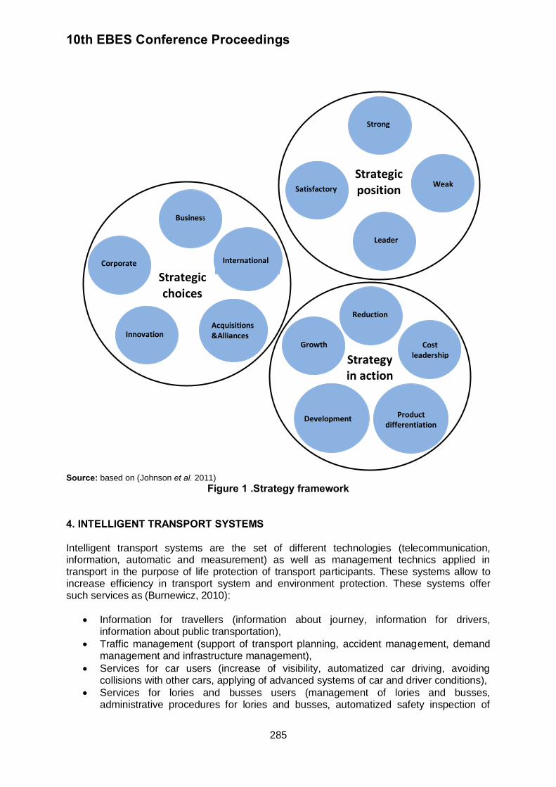
10th EBES Conference Proceedings
285
Source: based on (Johnson et al. 2011)
Figure 1 .Strategy framework 4. INTELLIGENT TRANSPORT SYSTEMS Intelligent transport systems are the set of different technologies (telecommunication, information, automatic and measurement) as well as management technics applied in transport in the purpose of life protection of transport participants. These systems allow to increase efficiency in transport system and environment protection. These systems offer such services as (Burnewicz, 2010):
Information for travellers (information about journey, information for drivers, information about public transportation),
Traffic management (support of transport planning, accident management, demand management and infrastructure management),
Services for car users (increase of visibility, automatized car driving, avoiding collisions with other cars, applying of advanced systems of car and driver conditions),
Services for lories and busses users (management of lories and busses, administrative procedures for lories and busses, automatized safety inspection of
Business
Strategic choices
Reduction
Strategy in action
Cost leadership
Growth
Development Product differentiation
Strong
Strategic position
Weak Satisfactory
Leader
Corporate International
Acquisitions &Alliances Innovation
10th EBES Conference Proceedings
286
vehicles, safety monitoring of vehicles with use of different appliances),
Services of public transport (management of public transportation, management of vehicles),
Help in case of danger (management of rescue teams, alert system connected with informing about dangerous materials),
Electronic toll collection (financial operation connected with payments),
Increase of infrastructure safety (intelligent crossroads). Intelligent transport systems support transportation system in Poland. There are some examples of applying such intelligent systems as access to satellite navigation on the base of GPS. Another example is “green wave” system in city traffic lights and electronic parking tickets. Practical examples are Warsaw trams management system and intelligent system of traffic management for mountain region. Development of intelligent transport system is supported by European union programs in the project “safety in transportation and national transportation network” in operational program “Infrastructure and Environment” for years 2007-2013.1 The aim of the program is to improve management of traffic through introducing intelligent transportation systems in road, sea, inland waterways as well as intermodal transportation and logistics. 5. INNOVATIVE ENERGETIC INFRASTRUCTURE OF TRANSPORT IN POLAND AND IN THE WORLD Innovative transport infrastructure is net of battery charging for electric cars (BEV) and net of compressed pure hydrogen refuelling for cars (FCV). Establishing of this net is necessary in the light of technological revolution in transport connected with changing traditionally fuelled cars with non-fossil fuelled cars. In many countries governments support the development of energetic infrastructure for transportation. In the years 2010 and 2012 there was a mass production of well-done and sold at good price electric cards there should be many station with changing and charging batteries. The number of charging stations is estimated about 5 million in 2015 all over the world. There will be about 1 million stations in the United States including private stations at homes. The biggest number of sold electric cars is in China, Japan and South Korea.2
Process of creation innovative transport infrastructure is possible because such companies like Better Place deal with environmental protection problems.3 Different companies try to develop new innovative transport infrastructure, which could be effective from economic and environmental point of view. 6. SUMMARY Polish transportation system is developing rapidly and it needs the European funding. It has been developed very well through last 20 years, even though there are many things to be done. Creation of strategic innovation in transport companies allows to build good position on the market. In today’s highly competitive transport industry markets, deciding how to al locate innovation sources with maximum impact has become increasingly challenging.
1 Operational Program “Infrastructure and Environment. National Strategic Framework for years 2007-2013
version from 3rd September 2009
http://www.pois.gov.pl/Dokumenty/Lists/Dokumenty20programowe/Attachments/93/SzOP_POIiS_v_3_2_30909.pdf”. 2 http://www.elektroda.pl/rtvforum/topic1692756.html [Accessed 08 March 2013]
3 http://www.betterplace.com/thecompany [Accessed 08 March 2013]
10th EBES Conference Proceedings
287
REFERENCES Bettencourt, L.A., Brown S.W., and Sirianni N.J., 2013. The secret to true service innovation. Business Horizons, 56(1), pp.13-22. Bogdaniecki, J., 2004. Innowacyjność przedsiębiorstw [Innovation of Enterprises]. Toruń:
Wydawnictwo University of Mikolaj Kopernik.
Burnewicz, J., 2010. Nowoczesna infrastruktura transportowa jako podstawowy element intensyfikacji procesów rozwojowych w projektowanych dokumentach strategicznych,
[Modern transport infrastructure as a basic element of intensification of development processes in projected strategic documents]. Expertise for Polish Ministry of Regional Development. Currie, W.L., 1999. Revisiting management innovation and change programmes: Strategic vision or tunnel vision? Omega, 27(6), pp.647-660.
Garcia, R. and Calantone R., 2002. A critical look at technological innovation typology and innovativeness terminology: A literature review. The Journal of Product Innovation Management, 19(2), pp.110-132.
Jaw, C., Lo, J.Y., and Lin, Y.H., 2010. The determinants of new service development: Service characteristics, market orientation, and actualizing innovation effort. Technovation, 30(4), pp.265–277.
Johnson, G., Scholes, K., and Whittington, R., 2011. Exploring Strategy Text & Cases. 9th
Edition. Essex: Prentice Hall.
Kalisz, D.E. and Aluchna, M., 2012. Research and innovation redefined. Perspectives on the European Union initiatives on horizon 2020. European Integration Studies, 6.
Matthyssens, P., Vandenbempt K., and Berghman L., 2006. Value innovation in business markets: Breaking the industry recipe. Industrial Marketing Management, 35(6), pp.751-761.
Stonehouse, G., Hamill, J., Campbell, D., and Purdie, T., 2001. Globalizacja. Strategia i zarzadzanie [Globalization. strategy and management]. Warszawa: Felberg SJA.
Tang, J., 2006. Competition and innovation behaviour. Research Policy, 35(1), pp.68–82.
Therrien, P., Doloreux D., and Chamberlin, T., 2011. Innovation novelty and (commercial) performance in the service sector: A Canadian firm – level analysis. Technovation, 31(12) pp.655–665.
Vries de, E.J., 2006. Innovation in services in networks of organizations and in the distribution of services. Research Policy, 35(7) pp.1037–1051.
10th EBES Conference Proceedings 23 - 25 May, 2013. NIPPON HOTEL, ISTANBUL, TURKEY ISBN: 978-605-64002-1-6. WEBSITE: www.ebesweb.org
288
FRANCHISING BETWEEN CONTROL AND AUTONOMY: WHAT IMPACTS ON INNOVATION?
KERIM KARMENI LaREMFiQ/LEM
University of Sousse/ University of Lille 1 Tunisia
OLIVIER DE LA VILLAREMOIS LEM
University of Lille 1 France
FAYSAL MANSOURI LaREMFiQ
University of Sousse Tunisia
Abstract: This research explores the impact of organizational control on innovation process via knowledge production and knowledge mobilization. This research used a qualitative approach in which five franchise network officers and two franchise experts were interviewed. Thematic analysis shows that behavior and social control are the most frequent mechanisms in the Tunisian franchise networks. We also find that these two control mechanisms play a crucial role in the innovation process, principally, by facilitating the management of organizational knowledge. Keywords: Franchising, Control, Organizational Knowledge, Innovation 1. INTRODUCTION Franchising is a form of commerce which plays an important role in the distribution and service sectors (Sorenson and Sørensen, 2001). This practice is considered as a form of distribution which has the fastest expansion scope in the world (Dant et al. 2011 ; Dant et al. 2008; Oxenfeldt and Thompson, 1969) and is frequently used as a strategy for internationalization (Cox and Mason, 2009). It is also recognized to have a positive impact on economy (Cumberland and Githens 2012; Dant et al. 2011; Dant et al.2008; Knight, 1986). This major advantage of franchising has attracted the attention of both practitioners and scholars (Madanoglu et al. 2011)
In addition to this economic and strategic role, franchising is qualified to be an important source of innovation: multiple authors stress on the role of franchisees on creativity and innovation (Bürkle and Posselt, 2008; Cox and Masson, 2007 ; Sorenson and Sørensen, 2001). Other scholars emphasize on the determinant role of franchisor in the innovation process mainly by validating new ideas and by diffusing the new concept on the franchise network (Davies et al. 2009 ; Cox and Masson, 2007). Innovation is not only determinant for
developing and attracting new franchisees but also necessary to maintain existing franchisees in the chain (Falbe et al. 1999).
10th EBES Conference Proceedings
289
Knowledge management is a way to succeed in innovation process (Nonaka, 1994). According to Nonaka (1994), an efficient system of knowledge management is a continuous and dynamic process that facilitates knowledge creation, acquisition, exploitation and memorization. Implementing a knowledge management system may face many problems: knowledge memorization (Darr et al. 1995), knowledge conversion (Lindblom and Tikkanen,
2010); knowledge transfer (Szulanski, 1996), etc. Face to these barriers, organizational control seems to play a critical role in facilitating knowledge management and stimulating innovation (Adler and Chen, 2011; Mundy, 2010, Poskela and Martinsuo, 2009 ; Turner and Makhija, 2006; La Villarmois et al. 2008; Ditillo, 2004 ; Simons, 1995). Based on the analysis grid proposed by La Villarmois et al. (2008), we conducted an
exploratory study in order to respond to the following research questions: what are the principal control mechanisms used in franchise network? In which way can organizational control affect knowledge management especially knowledge production and knowledge mobilization? The first main result is that information system; meeting and franchisees consultants (commercial agent) are frequently used in franchise networks. It means that the management of franchise network is mainly based on behavioral and social control mechanisms. A second outcome, research and development service, marketing service and franchisees suggestions appear to be the principal sources of innovation in franchise networks and the most used control mechanisms in knowledge management are behavioral and social. Finally, we concluded that interaction between control mechanisms and knowledge production/mobilization are facilitated by the combination of different types of control (initiatory, media model, evangelist and epidemic model). This paper starts a review of literature on principal topics: control of franchising network, the role of organizational control in innovation and presentation of analysis grid proposed by La Villarmois et al. (2008). Then, the paper describes methodology used to respond to forgoing
research questions. Eventually, the paper presents the main findings, limitations and recommendations for future research.
2. LITERATURE REVIEW 2.1. Control of franchise network
Franchising can be defined as a form of cooperation in which franchisor and franchisees share a part of their resources (brand name, management practices, knowledge, etc) while preserving autonomy (Azevedo, 2009). According to Michael and Combs (2008), franchising has received less attention by entrepreneurship scholars compared to novo startup or acquisitions. The authors stress that franchising constitutes an important source of entrepreneurship and it plays a positive role in the economy. The franchisees ’ level of autonomy is limited, because franchisor frequently imposes a control system in the chain to protect his brand name (Pizanti and Lerner, 2003). Chua and Mahama (2007) recognize that the success of interfirms cooperation depend on the implementing of appropriate mechanisms of control. In this paper, organizational control is seen as the combination of three control mechanisms: behavioral control, output control and social (clan) control (Turner and Makhija, 2006; Kirsch, 2004; Ouchi, 1977). The principal function of control is to influence people in the way that
10th EBES Conference Proceedings
290
facilitate the achievement of organization objectives (Kirsch, 2004; Anthony, 1988; Merchant, 1982). According to Dant and Nasr (1998), the establishment of control system within a franchise network is a very delicate operation: the need for autonomy must always be taken into account; it represents a fundamental motivation for the franchisees to join a network. The legal autonomy of franchisees implies a loss of control for the franchisor and consequently the success of the franchise system requires compensation for this loss of control by establishing specific mechanisms (Cochet et al. 2008). Frazer et al. (2007) argue that
inappropriate balance between coercive sources of power (contractual obligations, legal action) and non coercive sources of power (reward system) can engender the disruption of the franchise relationship. Theses researches illustrate the key role of control in the franchise network. The concept of control is frequently associated with the management of plural form (Mellewigt et al. 2011; Bradach, 1997), the minimizing of opportunism behavior (Agency
theory) (Boulay, 2010 ; Jambulingam and Nevin, 1999 ; Dant and Nasr, 1998), internationalization via franchising (Wang and Altinay, 2008 ; Doherty and Alexander, 2006; Gannon and Johnson, 1997) and the balance between standardization and adaptation or exploitation and exploration (Cox and Masson, 2007; Pizanti and Lerner, 2003; Lewin, 1999). A new research avenue is inspired by the levers of control framework (Simons, 1995): deepening the role of the control system in the knowledge management and innovation. Thus the effect of control mechanisms on organizational knowledge and innovation has to be looked at especially in franchise networks. 2.2. The role of control system in innovation
Innovation is the successful introduction of a new product or service, a new method or new practices or techniques (Dasgupta and Gupta, 2009; Damanpour, 1991). These operations contribute in the creation of value for the organization and its stakeholders (Dasgupta and Gupta, 2009). For Popadiuk and Choo (2006), the success of an innovation depends on two criteria: the transformation of an idea into a new product or service and the commercialization of this product or service. Two main typologies of innovation can be distinguished. The first one is based on the level of change introduced:
radical innovation: for Plessis (2007), radical innovation constitutes a rupture with
existing practices (products, services, technologies applied) and is always associated with a high level of risk due to the difficulties of commercialization of new products or services.
incremental innovation: incremental innovation can be defined as an adjustment to
existing products / services that will keep existing practices and helps to develop the expertise available within the organization (Plessis, 2007). The second typology is based on the innovation’s object:
product innovation: product innovation is assimilated to the development of new
products or services to reach the market demand (Damanpour, 1991; Utterback and Abernathy, 1975);
process innovation : process innovation is related to the development of new
techniques or methods of production like the introduction of new input materials, new task specification, new equipments used in production, etc. (Damanpour, 1991; Utterback and Abernathy, 1975).
According to Cumberland and Githens (2012), the interaction of franchisees with customers and their direct involvement in activity allow them to cumulate a critical mass of tacit knowledge and influence their sense of creativity. Cumberland and Githens (2012) notice

10th EBES Conference Proceedings
291
that resolving problems related to the tacit knowledge transfer, can support innovation within the franchise network. Innovation also can be described as a form of organizational knowledge creation (Nonaka, 1994). The author defines organizational knowledge as the process by which an organization promotes exchanges and interaction between its members in order to develop the knowledge created by individuals. He states that the creation of knowledge can also be generated in the context of inter-organizational interaction. In this context, the control mechanisms also play an important role in knowledge management. The question on the role of control in innovation receives more and more attention by researchers, however, there is not yet a clear answer to this question (Bisbe and Otley, 2004). In order to assess the role of control mechanisms in the innovation process, Poskela and Martinsuo (2009) examine the critical phase that precedes the development of a new product (the front end of innovation). This preliminary phase focuses on the study of innovation feasibility and its compliance with the strategic objectives of the company. By analyzing several types of control mechanisms, Poskela and Martinsuo (2009) show that outcome control and behavioral control (the formalization of procedures) play no significant role in the management of innovation, especially in a long-term perspective. While the input control (control over resources, planning) and the intrinsic task motivation are determinants in the front end innovation. The result shows that these two types of control (input control and intrinsic task motivation) play an important role in managing the tension between the need for innovation and achieving the strategic renewal of the organization. Following their theoretical analysis on the relationship between control and the process of knowledge management, Turner and Makhija (2006) suggest the following proposals:
outcome control is the best suited with the interpretation phase of knowledge. It also allows using knowledge in an original way.
social control facilitates the creation and acquisition of new knowledge. It also helps to promote the transfer of knowledge between different members of the organization and it is also very useful for the interpretation phase of knowledge. In addition, social control allows an adapted use of organizational knowledge.
behavioral control induces a tight application of knowledge. The results reported in literature are varied: the analysis of previous results helps to develop learning within the firm (Merchant, 1982), the interactive use of control system stimulates learning and innovation (Simons, 1995), the control mechanisms which promote autonomy support exploratory learning (McGrath, 2001), control mechanisms play a key role in knowledge production and mobilization (La Villarmois et al. 2008).
In a different perspective, authors have rejected the significant role of control in innovation: unlike the analysis of Simons (1995), the results of the study of Bisbe and Otley (2004) show no significant relationship between interactive use of formal control and innovation. The authors conclude that the interactive use of formal control system plays a moderating role between innovation and organizational performance. Damanpour (1991) shows no significant effect between innovation and formalization which means that behavioral control has no significant role in innovation. In a similar process, Sorenson and Sørensen (2001) see that behavioral control and outcomes control are used to maintain standardization and disadvantage innovation.

10th EBES Conference Proceedings
292
These findings show that there is not yet a consensus on the relationship between control and innovation. In the following part, we present the framework which was used in the empirical part.
2.3. An analysis grid for the interaction between control mechanisms and organizational knowledge
Control mechanisms are considered to be key factors for organizational learning and in particular in the knowledge acquisition, transfer, memorization, use and in the transformation of individual knowledge into organizational knowledge. Based on their study of multinational firms, La Villarmois et al. (2008) proposed an analytical framework that describes the role of
various control mechanisms in the production and mobilization of knowledge on the local and global level. The framework describes four principal models:
Knowledge production by the control system
Knowledge mobilization
Global Local Global Box 1: The media model
ERP, CRM and SCM The integration of information systems enables global knowledge to be produced and circulated, erasing any local specificities, which will be mobilized in the same way. Knowledge is mediatized by technology.
Box 2: The initiatory model Studies carried out by head office Studies carried out by head office (global production) are circulated to all the subsidiaries. Each one interprets them to its own local situation. Global knowledge is adapted.
Local Box 3: The evangelist model Identification of best practices The development process of a product used by a subsidiary (local production) is used by all subsidiaries (global mobilization). The best practice, once identified, will be the good word spread throughout the organization.
Box 4: The epidemic model Benchmarking Exchanges between subsidiary managers, within a benchmarking process, could mean that a locally developed practice could be used elsewhere, but always in a local context. Contagious circulation could be more or less widespread.
Source: La Villarmois et al. (2008,p.149) Figure1: Analysis grid of interaction between control and production/mobilization of
knowledge the media model: media model is the intersection between global production and global
mobilization of knowledge. This model is essentially based on the information system as (ERP, CRM, SCM ...);
the initiatory model: initiatory model is the process resulting from the intersection
between global production and local mobilization of knowledge. This model describes the role of the control system in the adaptation of local knowledge;
the evangelist model: evangelist model describes the process of identifying local best
practices and their diffusion throughout the network. It represent the intersection between the production of local knowledge and its mobilization at the global level;
the epidemic model: the epidemic model is the process resulting from the intersection
between the local production and mobilization of knowledge. This model is based on the

10th EBES Conference Proceedings
293
practice of "benchmarking" and describes the practices of exchanges between the subsidiary managers.
This grid will allow us to analyze the different control mechanisms observed in franchise networks and classify the different configurations of interaction between control mechanisms and the two determinant steps of knowledge management (knowledge production and knowledge management). 3. RESEARCH METHODOLOGY Due to the exploratory nature of this study, we adopt a qualitative approach in the current research stage. Data collection is done through semi-structured interviews conducted with franchise experts and officials of franchise networks, internet, visit of franchise exhibition "Tunis-MedFranchise" (Table 1). First, semi-structured interviews conducted with managers and franchise expert have enabled us to identify control practices applied in the management of franchise networks which were useful to analyze the role of control in the management of organizational knowledge. Then various information on the characteristics of franchise networks studied were collected across websites. Finally, the interventions in the show franchise have been helpful in clarifying the current situation for franchising in Tunisia because this practice is still in its early stages of development. Networks studied (Tunisiana, Chahia, Masmoudi and City Sport) are selected due to their high implication in franchise activities in Tunisia and also due to the acceptance of franchisor to participate in this study.
Table 1. List of interviews List of interviews Function of interviewee Interviewing
instrument interview 1 Franchise manager in Tunisiana network annotation interview 2 Sales manager in Tunisiana network recording interview 3 Commercial director of Chahia network recording interview 4 Responsible for export in Masmoudi
network recording
interview 5 Director of national development in City sport network
recording
interview 6 (Expert A)
CEO of a consulting firm "francounselgroup”
recording
interview 7 (Expert B)
CEO of a consulting firm “Occasion franchise”
recording
Based on the theoretical background related to the principal notion of this study (franchise networks, control, innovation, knowledge management) we begin by developing a grid interviews, then we conducted different interviews with records except in one case where we took notes. Finally, the interviews were transcribed in order to start the content analysis. We adopt a thematic analysis technique (analysis of meaning) which is based on cutting, coding and analysis of the text according to specific themes. 4. EMPIRICAL RESULTS AND DISCUSSION The studied networks are presented in Table 2. The analysis of interviews conducted with two international franchise experts (Expert A and Expert B) and five franchise networks officers allowed us to distinguish between three principal themes around which the interviews were held:
Theme 1 : general information on the monitoring tools and innovation in franchise networks;
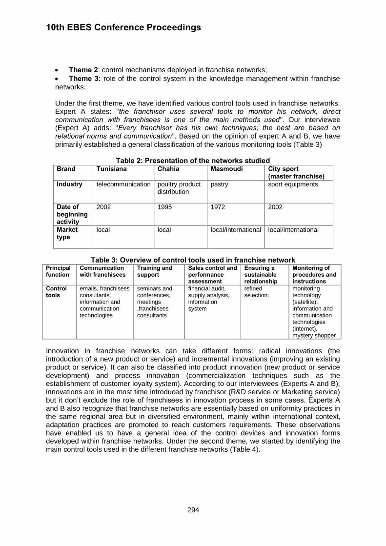
10th EBES Conference Proceedings
294
Theme 2: control mechanisms deployed in franchise networks;
Theme 3: role of the control system in the knowledge management within franchise
networks. Under the first theme, we have identified various control tools used in franchise networks. Expert A states: "the franchisor uses several tools to monitor his network, direct communication with franchisees is one of the main methods used". Our interviewee (Expert A) adds: "Every franchisor has his own techniques; the best are based on relational norms and communication". Based on the opinion of expert A and B, we have
primarily established a general classification of the various monitoring tools (Table 3)
Table 2: Presentation of the networks studied Brand Tunisiana Chahia Masmoudi City sport
(master franchise) Industry telecommunication poultry product
distribution
pastry sport equipments
Date of beginning activity
2002 1995 1972 2002
Market type
local local local/international local/international
Table 3: Overview of control tools used in franchise network
Principal function
Communication with franchisees
Training and support
Sales control and performance assessment
Ensuring a sustainable relationship
Monitoring of procedures and instructions
Control tools
emails, franchisees consultants, information and communication technologies
seminars and conferences, meetings ,franchisees consultants
financial audit, supply analysis, information system
refined selection;
monitoring technology (satellite), information and communication technologies (internet), mystery shopper
Innovation in franchise networks can take different forms: radical innovations (the introduction of a new product or service) and incremental innovations (improving an existing product or service). It can also be classified into product innovation (new product or service development) and process innovation (commercialization techniques such as the establishment of customer loyalty system). According to our interviewees (Experts A and B), innovations are in the most time introduced by franchisor (R&D service or Marketing service) but it don’t exclude the role of franchisees in innovation process in some cases. Experts A and B also recognize that franchise networks are essentially based on uniformity practices in the same regional area but in diversified environment, mainly within international context, adaptation practices are promoted to reach customers requirements. These observations have enabled us to have a general idea of the control devices and innovation forms developed within franchise networks. Under the second theme, we started by identifying the main control tools used in the different franchise networks (Table 4).

10th EBES Conference Proceedings
295
Table 4: Summary of control tools used in franchise networks Chain Tunisiana Chahia Masmoudi City Sport Control tools
refined selection, information system, financial audit, franchise contract, book of specifications, organizational charter, commercial agent, mystery shopper, training, meeting.
information system, communication tools (call center and posters), financial incentives, commercial agent, relational norms (confidence), training, meeting.
information system, communication tools (posters and catalogs, call center), franchise contract, operational manual, supply monitoring, specific machines, franchisees consultant, training, meeting.
information system, franchise contract, operational manual, supply monitoring, relational norms (confidence), franchisees consultant, meeting.
Based on table 4, we observe that information system, meeting and franchisees consultants are the most used tools in monitoring franchise networks. We also can note the absence of use of customer satisfaction assessment as a control tool in Tunisian franchise networks although it is considered to be important in franchise networks monitoring (Dant and Nasr, 1998). On the other hand, we notice the lack of accounting tools such scorecard or budget although they are considered as the key mechanisms of management control (Bisbe and Otley, 2004). This may be due to the specific form of control in franchise networks: the relationship between the controller and the controlled is characterized by legal independence, which makes the franchisor choose the application of non-classical control mechanisms. Subsequently, we classified the various monitoring tools which were identified into three main categories: behavioral control mechanism, outcome control mechanism and social control mechanism (Table 5).This classification is made with reference to the different information we have collected and based on the literature. Then, based on the distribution of the different control mechanisms (Table 5), we observe a clear dominance of behavioral and social control. The low use of outcome control mechanisms can be explained by the low level of uncertainty for the studied activities. Outcome control is generally used in an environment where the level of uncertainty is high or when activities are constituted by complex tasks (Turner and Makhija, 2006; Ouchi, 1980). Finally, we find that the studied networks use control in an interactive and complementary way (combine between more than control tool). We also note a strong association between the use of behavioral control and social control. Analysis of the last theme allowed us to examine the interaction of control mechanisms with knowledge management (knowledge production and knowledge mobilization) by applying the grid analysis of La Villarmois et al. (2008). Table (6) summarizes the main findings emerged from the latter stage of this study.

10th EBES Conference Proceedings
296
Table 5: Control mechanisms in franchise network Chain Control tools Type of control mechanism Tunisiana
refined selection social control information system behavioral control training behavioral control/social control meeting behavioral control/social control financial audit behavioral control contract behavioral control book of specifications behavioral control organizational charter social control chef de zone behavioral control/social control mystery shopper behavioral control
Masmoudi
information system behavioral control communication tools (call center)
behavioral control/social control
meeting behavioral control/social control training behavioral control/social control specific machine behavioral control contract behavioral control operational manual behavioral control supply monitoring behavioral control franchisees consultant behavioral control/social control
Chahia
information system behavioral control communication tools behavioral control/social control meeting behavioral control/social control training behavioral control/social control financial incentives outcome control commercial agent behavioral control/social control relational norms (confidence) social control
City sport
information system behavioral control meeting behavioral control/social control contract behavioral control operational manual behavioral control relational norms (confidence) social control supply monitoring behavioral control franchisees consultant behavioral control/social control

10th EBES Conference Proceedings
297
Table 6: Main findings Tunisiana Chahia Masmoudi Citysport Forms of innovation
radical and incremental
product innovation
radical and incremental
product innovation
radical and incremental
product innovation
radical and incremental
product and process innovation
Innovation sources
R&D service Marketing service and franchisees
Marketing service and franchisees
franchisor and franchisees
Knowledge production and knowledge mobilization
knowledge production is related to R&D service which is established in head office (global production);
knowledge is mobilized in all network without local adaptation (global mobilization);
knowledge is produced globally (by franchisor) and locally by franchisees;
knowledge is mobilized in all network without local adaptation (global mobilization);
knowledge is produced globally (by franchisor) and locally by franchisees;
knowledge is mobilized locally for international units and globally for local units;
knowledge is produced globally (by franchisor) and locally by franchisees;
knowledge is mobilized in all network without local adaptation (global mobilization);
Control mechanisms used in knowledge management
behavioral and social control (information system, meeting, training, commercial agent)
behavioral and social control (communication tools, meeting, franchisees consultant)
behavioral and social control (communication tools, meeting, franchisees consultant)
behavioral and social control (communication tools, meeting, confidence)
Application of analysis grid: interaction between control and knowledge management
The media model
combination between media and evangelist models
combination between media and evangelist models for local units;
combination between media, evangelist and initiatory models for international units;
combination between media and evangelist model
5. CONCLUSION In this study, we started with a general analysis of the management of franchising networks which has allowed us to identify and understand the function of the different monitoring tools. We also found that knowledge is produced on two levels (local/franchisees and global/franchisor) while knowledge mobilization is primarily done in the global level except in the case of international networks. Then, we could classify the different control tools used in franchise networks into three main categories: behavioral control mechanisms, outcome control mechanisms and social control mechanisms. Finally, the analysis of the interaction between knowledge production and knowledge mobilization on one hand and control mechanisms on the other hand allowed us to generate the following results:
behavioral and social control mechanisms play an important role in knowledge production and knowledge mobilization: tools like communication, meeting and training are used for
10th EBES Conference Proceedings
298
knowledge production and tools like information system, franchisee consultant or commercial agent, training, meeting, confidence are used for knowledge mobilization. Therefore, these forms of control are determinant in innovation development;
research and development service, marketing service and franchisees suggestions are the main sources of innovation in franchise networks;
knowledge is produced in global and local level while knowledge mobilization mainly occurred at global level except in the case of internationalization;
interaction between controls mechanisms and knowledge management can be resumed in different combinations of initiatory model, media model, evangelist model and epidemic model.
Some limits must be recognized: first, focusing on knowledge production and knowledge mobilization, we have not paid enough attention to determinants of innovation like specialization, managerial attitude toward change, slack resources, etc (Damanpour, 1991), codification of knowledge (Nonaka, 1994), and tension between exploration and exploitation (March, 1991). Second, we have discarded the franchisees in this investigation even though they constitute a main source for innovation. Third, the number of interviews is limited. This work can be developed in the context of a cross-cultural study while expanding data sources in order to generalize the results. A quantitative analysis can also be considered to this research in order to confirm the results related to the interaction between control and innovation. REFERENCES Adler, P.S. and Chen, C.X., 2011. Combining creativity and control: Understanding individual motivation in large-scale collaborative creativity. Accounting, Organizations and Society, 36(2), pp.63-85. Anthony, R.N., 1988. The management control function. Boston, Mass: Harvard Business
School Press. Azevedo, P.F., 2009. Allocation of authority in franchise chains. International Studies of Management and Organization, 39(4), pp.31-42.
Bisbe, J. and Otley, D., 2004. The effects of the interactive use of management control systems on product innovation. Accounting, Organizations and Society, 29(8), pp.709–737.
Boulay, J., 2010. The role of contract, information systems and norms in the governance of franchise systems. International Journal of Retail and Distribution Management, 38(9),
pp.662-676. Bradach, J.L., 1997. Using the plural form in the management of restaurant chains. Administrative Science Quarterly, 42(2), pp.276-303.
Bürkle, T., and Posselt, T., 2008. Franchising as a plural system: A risk-based explanation. Journal of Retailing, 84(1), pp.39-47.
Chua, W. F. and Mahama, H., 2007. The effect of network ties on accounting controls in a supply alliance: Field study evidence. Contemporary Accounting Research, 24(1), pp.47-86.

10th EBES Conference Proceedings
299
Cochet, O. and Garg, V.K., 2008. How do franchise contracts eve? A study of three German SMEs. Journal of Small Business Management, 46(1), pp.134–151.
Cox, J. and Mason, C., 2009. Franchise network restructuring: Pressures, constraints and mechanisms. Entrepreneurship and Regional Development, 21(5-6), pp.503–527.
Cox, J. and Mason, C., 2007. Standardization versus adaptation: Geographical pressures to deviate from franchise formats. The Service Industries Journal, 27(8), pp.1053-1072.
Cumberland, D. and Githens, R., 2012. Tacit knowledge barriers in franchising: Practical solutions. Journal of Workplace Learning, 24(1), pp.48-58.
Damanpour, F., 1991. Organizational innovation: A meta-analysis of effects of determinants and moderators. Academy of Management Journal, 34(3), pp.555-590. Dant, R.P. and Nasr, N.I., 1998. Control techniques and upward flow of information in franchising in distant markets: Conceptualization and preliminary evidence. Journal of Business Venturing, 13(1), pp.3-28.
Dant, R.P., Grünhagen, M., and Windsperger, J., 2011. Franchising research frontiers for the twenty-first century. Journal of Retailing, 87(3), pp.253-268.
Dant, R.P., Perrigot, R., and Cliquet, G., 2008. A Cross-cultural comparison of the plural forms in franchise networks: United States, France, and Brazil. Journal of Small Business Management, 46(2), pp.286-311.
Darr, E.D., Argote, L., and Epple, D., 1995. The Acquisition, transfer, and depreciation of knowledge in service organizations: Productivity in franchises. Management Science, 41(11),
pp.1750-1762. Dasgupta, M. and Gupta, R., 2009. Innovation in organizations: A review of the role of organizational learning and knowledge management. Global Business Review, 10(2),
pp.203-224. Davies, M. A., Lassar, W., Manolis, C., Prince, M., and Winsor, R.D. 2009. A model of trust and compliance in franchise relationships. Journal of Business Venturing, 26(3), pp.321-340.
Ditillo, A., 2004. Dealing with uncertainty in knowledge-intensive firms: The role of management control systems as knowledge integration mechanisms. Accounting, Organizations and Society, 29(3-4), pp.401-421.
Doherty, A.M. and Alexander, N., 2006. Power and control in international retail franchising. European Journal of Marketing, 40(11-12), pp.1292-1316.
Falbe, C.M., Dandridge, T.C., and Kumar, A., 1999. The effect of organizational context on entrepreneurial strategies in franchising. Journal of Business Venturing, 14(1), pp.125-140.
Frazer, L., Merrilees, B., and Wright, O. 2007. Power and control in the franchise network: An investigation of ex-franchisees and brand piracy. Journal of Marketing Management, 23(9-
10), pp.1037-1054.
10th EBES Conference Proceedings
300
Gannon, J., and Johnson, K. 1997. Socialization control and market entry modes in the international hotel industry. International Journal of Contemporary Hospitality Management , 9(5-6), pp.193-198. Jambulingam, T. and Nevin, J.R., 1999. Influence of franchisee selection criteria on outcomes desired by the franchisor. Journal of Business Venturing, 14(4), pp.363-395.
Kirsch, L.J., 2004. Deploying common systems globally: The dynamics of control. Information Systems Research, 15(4), pp.374-395.
Knight, R.M., 1986. Franchising from the franchisor and franchisee points of view. Journal of Small Business Management, 24(3), pp.8-15. La Villarmois, O.D., Benavent, C., and Firmanzah, F., 2008. control and organizational learning in MNCs: An analysis through the subsidiaries. The South East Asian Journal Management, 2(2), pp.133-154.
Lewin, S.B., 1999. Innovation and authority in franchise systems: An empirical exploration of the plural form. Working Paper, University of Cambridge.
Lindblom, A. and Tikkanen, H., 2010. Knowledge creation and business format franchising. Management Decision, 48(2), pp.179-188.
Madanoglu, M., Lee, K., and Castrogiovanni, G.J., 2011. Franchising and firm financial performance among U.S. restaurants. Journal of Retailing, 87(3), pp.406-417.
McGrath, R.G., 2001. Exploratory learning, innovative capacity and managerial oversight. The Academy of Management Journal, 14(1), pp.118-131.
Mellewigt, T., Ehrmann, T., and Decker, C., 2011. How does the franchisor’s choice of different control mechanisms affect franchisees’ and employee-managers’ satisfaction? Journal of Retailing, 87(3), pp.320-331.
Merchant, K.A., 1982. The control function of management. Sloan Management Review, 23(4), pp.43-55. Michael, S.C. and Combs, J.G., 2008. Entrepreneurial failure: The case of franchisees. Journal of Small Business Management, 46(1), pp.73-90.
Mundy, J., 2010. Creating dynamic tensions through a balanced use of management control systems. Accounting, Organizations and Society, 35(5), pp.499-523. Nonaka, I., 1994. A dynamic theory of organizational knowledge creation. Organization Science, 5(1), pp.14-37. Ouchi, W.G., 1977. The relationship between organizational structure and organizational control. Administrative Science Quarterly, 22(1), pp.95-113. Oxenfeldt, A.R. and Thompson, D.N., 1968/1969. Franchising in perspective. Journal of Retailing, 44(4), pp.3-11.

10th EBES Conference Proceedings
301
Pizanti, I. and Lerner, M., 2003. Examining control and autonomy in the franchisor–franchisee relationship. International Small Business Journal, 21(2), pp.131-159.
Plessis, M. d., 2007. The role of knowledge management in innovation. Journal of Knowledge Management, 11(4), pp.20-29.
Popadiuk, S. and Choo, C.W., 2006. Innovation and knowledge creation: How are these concepts related? International Journal of Information Management, 26(4), pp.302-312.
Poskela, J. and Martinsuo, M., 2009. Management control and strategic renewal in the front end of innovation. Journal of Product Innovation Management, 26(6), pp.671-684.
Simons, R., 1995. Levers of control: How managers use innovative control systems to drive strategic renewal. Boston: Harvard Business School Press. Sorenson, O. and Sørensen, J.B., 2001. Finding the right mix: Franchising, organizational learning, and chain performance. Strategic Management Journal, 22(6-7), pp.713–724. Szulanski, G., 1996. Exploring internal stickiness: Impediments to the transfer of best practice within the firm. Strategic Management Journal, 17, pp.27-43. Turner, K.L. and Makhija, M.V., 2006. The role of organizational controls in managing knowledge. Academy of Management Review, 31(1), pp.197-217.
Utterback, J.M. and Abernathy, W.J., 1975. A dynamic model of process and product innovation. Omega, 3(6), pp.639-656.
Wang, C.L. and Altinay, L., 2008. International franchise partner selection and chain performance through the lens of organizational learning. The Service Industries Journal, 28(2), pp.225-238.
10th EBES Conference Proceedings 23 - 25 May, 2013. NIPPON HOTEL, ISTANBUL, TURKEY ISBN: 978-605-64002-1-6. WEBSITE: www.ebesweb.org
302
NON-EU EURASIA INVESTMENT FOR RESIDENCE: THE LATVIAN WAY
ANDREJS LIMANSKIS
Department of economics and finance Riga International School of Economics and Business Administration-RISEBA
Latvia [email protected]
Abstract: Investment attraction programs constitute a new phenomenon in international business. This research extends theory and practice of attraction of foreign capital. It investigates the determinants of innovative program by Latvia providing non-EU foreigners, mainly Eurasians, with residence permits in exchange for investments. The aim of this empirical research is to test hypothesis that Residence Permits for Investment program in Latvia can be viable and successfully implemented in attraction of Eurasian investors. Qualitative and quantitative methods, including macro- and micro-economic analysis and questioning of stakeholders are to be used. No unit of analysis has been published in Latvia or globally. This article is an attempt to start scientific discussion. Methods of analysis are to be tested. As result of empirical research, trend in capital attraction is quantitatively measured, motives of non-EU Eurasian investors generalized for perfection of the program. It is concluded that readiness to invest in Latvian economy is raising but should be supported by creative actions of the governments both nationally and internationally. Research paves the way for Recipient States Attractiveness Index for Foreign Investors. There is room for improvement in teaching International Business at institutions of higher education. Keywords: Residence Permits for Investment, Eurasian Investment in Latvia, Recipient
State. 1. INTRODUCTION Investment programs available with different countries in Eurasia constitute a new phenomenon in international business and economics. Since 2010 when Latvian Saema adopted and President of Latvian Republic signed innovative Amendments to the Law on Immigration of 2002 (2010), international business community, researchers and politicians are involved in discussion of different aspects of this matter. For the first time since restoration of political independency of Latvia, non-EU citizens have been granted an opportunity to qualify for temporary residence permit (TRP) in Latvia. A TRP allows visa-free movements in the Schengen zone. Non-EU investors are invited to input in the economic development of an EU (and NATO) member state in order to obtain TRP for themselves and members of their families. In the context of geographical position of Latvia the program „TRP for investment” turns to be focused on citizens of Eurasia but is open for any non-EU national. At the moment no unit of analysis of the phenomenon has been published either in Latvia, or globally. This article is an attempt to start research in the topic and give material to scientific discussion. Methods of analysis are a crucial point to be tested, discussed and corrected if necessary. In Turkey as in the majority of states of Eurasia there is no such program. Foreigners wishing to live and/or work in Turkey are required to obtain a residence permit within one month following their arrival in the country and prior to the commencement of their work. For long-
10th EBES Conference Proceedings
303
term residence in Turkey, the applicant should submit passport and a bank statement to the local Police Department, namely bank statement or a currency exchange slip testifying to an asset in the amount of USD 300 for each month. Advantages of Latvian residence permits are many, including free travelling in Schengen area (residence permit allows staying in Schengen member states without visa), long validity period (a residence permit issued under making investments is valid for the period up to 5 years), no limitations on residing in Latvia (unlike many other Schengen states, Latvia does not require persons granted a residence permit to stay in Latvia permanently. At the same time, after obtaining a residence permit one can live in Latvia all the year round) and relocation opportunity (if a family or some of the family members consider an opportunity to move to Europe in future, a residence permit obtained in the European Union member state and residing there will be treated as a plus when applying for a status of permanent resident or citizen in some EU member state). The extreme depth of economic crisis in Latvia in 2008 compared to the EU average proves weakness of former economic strategies irresponsive of the general sicknesses of political and financial system that triggered the crisis. Certain success of Latvia in overcoming the crisis attracted attention of Nobel Prize winner Krugman (2013) who made macroeconomic research and raised voice against praising Latvian government for so called internal devaluation of the local currency. Prospect of introduction of euro in Latvia in 2014 adds to discussion on feasibility and viability of such programs as TRP for investment in mid-term. As Reuter's analysts Wheatley and Tapinsh (2013) notice, Brussels and Frankfurt are concerned that the Latvian banking system's big pool of non-resident deposits is a source of financial vulnerability, as it is in Cyprus. Prime Minister of Latvia Dombrovskis uses to brush aside the comparison with Cyprus and to underline Latvia meets the euro zone's economic criteria. But the discussion is far from being completed. Against this background, the aim of this empirical research is to test hypothesis that Residence Permits for Investment program in Latvia can be viable and successfully implemented in attraction of Eurasian investors. 2. RESEARCH METHODOLOGY Recently, the concept of acceleration of foreign direct investment (FDI) as strategic means of development of an economy under post-crisis situation has received an increased attention. The concept refers to the idea of stimulating foreign investors to participate in economic revival of a country without questioning the foundations of the economic and political system of the host and the donor country. Especially, sticking to the democratic model in politics and the market economy model in economics is to be joined with inflow of capital from previously rejected source. In case of Latvia, inflow of capital from Russia, territorially the largest in Eurasia, suffers tradition of suspicious acceptance as stemming from Imperial state of immature democracy and state-dominated oligarchical model of market economy. Minister of Economy of Latvia Pavluts (2012) at Russia-Latvia economic cooperation conference opposed anti-Russian sentiments as concerns TRP program and noticed that “all is not so simplistic and flat”. So it is important to investigate if there is a tendency in the TRP issue to Eurasia citizens by years since the start of the program and if the suspicious acceptance has grounds. To deepen the research it is high time to investigate which of the three forms of investment in the framework of the TRP program is most attractive for non-EU Eurasian citizens.
10th EBES Conference Proceedings
304
2.1. Limitations of the research First, the TRP for investment in Latvia program is running since 1.07.2010. Hence the research horizon is rather narrow and preciseness of forecasts cannot be great. Nevertheless the author has performed collection of data during rather a long period and arrived to conclusion that in the beginning of 2013 the first investigation can be substantiated as reliable to acceptable level. Second, structure of adopted non-EU applications for TRP in Latvia has been published officially only once (5.11.2011) for information of the Saema. Structure of Eurasia countries of origin of investments done for obtaining the TRP in Latvia was not disclosed for wider academic use. There is need to make certain assumptions and correct them in accordance with new publications of statistics and arrival of additional evidence. Third, Latvian statistics is measuring FDI in local currency Lats (LVL). 1.01.2014 is planned to be the date of introduction of the euro (EUR) in Latvia if the fulfillment of Maastricht criteria is accepted by the European commission. Experience of transition of Estonia from Estonian krona to euro in 2012 and of Slovakia from Slovak krona to euro in 2008 demonstrated two possible scenarios. One is transition to euro without revaluation of local currency against euro (Estonian way) and the second is transition to euro with previously done revaluation of local currency (Slovak way). For Latvia there is short opportunity to perform revaluation of Lats in the first half of 2013 before transition to euro. This research employs the official peg, i.e. exchange rate set for Latvia in 2005 at 0,702804 Lats for 1 EUR with the corridor +/- 1%. At the final day of this investigation there is statement by Bank of Latvia that precisely this exchange rate will be used for transition to euro. However one is to be ready to recalculate values in case of change in the exchange rates. Fourth, during this research some follower EU states announced similar programs to attract additional investment, namely Bulgaria, Romania and Spain. It can affect applications for Latvian TRPs from citizens of a number of non-EU states of Eurasia. But the impact cannot be measured yet. One more alternative-sham marriages-is also excluded from this research despite the fact that only in Ireland according to Baltic Times (2013) in 2012 Latvian citizens registered 108 marriages with third country citizens which visibly increases TRP issues in such small country as Latvia. Fifth, many non-EU middle-class representatives of Eurasia states already have investments done globally. So investment opportunity for TRP in Latvia may be not attractive for majority of them since they already got used to visa system in Schengen zone and can enjoy multi-visas issued for periods up to five years. 2.2. Literature review and methods of analysis Attraction of FDI from donor to recipient countries is one of the hottest areas of research in international business. According to Hill (2009), championing in International Business textbooks, recipient states never find it easy politically to open the country to FDI and keep being open. Advantages of attracting foreign capital go hand in hand with disadvantages making equilibrium hard to be sustained. Nevertheless, as Francis and Ibbotson (2002) dared to suggest, international investing increases despite the fact that it involves all the risks associated with domestic investing, plus additional risks. The Economist analyst (2013) was the first to wonder about the implications of the Cyprus bail-out deal of 16.03.2013 for little Latvia, also home to lots of Russian money and itself due
10th EBES Conference Proceedings
305
to join the euro zone in 2014. Geographically, according to the 2011 forecast by Economist Intelligence Unit (2007), Latvia is not covered at all as recipient of FDI. Nor Latvia can be found among figurants of the Center for Global Development Commitment to Development Index (2012) famous for measuring seven non-weighted factors, although territorially smaller Slovakia is there. There is no monograph yet devoted to the topic of TRP in Latvia or any other EU state for investments. In Internet one comes across list of EU states (Austria, Belgium, UK, Bulgaria, Latvia, Czech Republic) where it is possible in 2013 to reside by investing. But there is no research of the topic internationally. Basic sources of TRP issue for investment in Latvia are official statistics and press releases by Bank of Latvia (2012), Central statistical bureau of Latvia CSB (2012) and Citizenship and Migration Authority LNMP (2012). They all started to emerge recently. Latvian politicians without preliminary research publications have amended a threshold figure of the already running program, namely doubled the size of investment in the capital of companies in Latvia as minimum to qualify for TRP. International writers started to investigate different aspects of the topic in late 2012. The New York Times author Gregor (2012) generalized information on real estate in Latvia as potential for foreign investors. Some figures on TRP issue have been reprinted by The Baltic Times (2013), namely the number of apartments bought in 2012 in Riga and Jurmala. Simultaneously alternative investment opportunities in the capital of companies or in the subordinated capital of banks in Latvia were mentioned. Proper attention is paid to prevention of money laundering in Latvia in the Laws of Latvian Republic especially in conjunction with Real Estate deals disclosed by Nira Fonds (2013) in one of the first publication of corresponding data. Three Latvian companies headed by Baltic Sotheby`s International Realty (2012) published parts of research in the social portrait of non-EU investor seeking for TRP in Latvia. Perception of BRICs businessmen abroad investigated by the Economist Intelligence Unit (2012) ordered by RUSAL did not take into account the investment for TRP issue. At the moment no attempt of analysis of the quantitative indicators of the phenomenon has been published neither in Latvia, Eurasia or globally. Even recent international conferences tend to ignore the TRP for investment program in official schedules. This article is an attempt to spread research in the topic internationally and give a start to international scientific discussion. Methods of analysis are a crucial point to be tested, discussed and corrected if necessary. International comparisons are to be facilitated. Research question 1 is if there is a tendency in the TRP issue by years since the start of the program. Answering to this question demands thorough collection of statistics from all possible sources and plotting an analytical table. Use of MS EXCEL software is instrumental because, first, it facilitates introduction of updates in statistics, and, second, provides for in-depth investigation of time series and comparisons. This type of research is quantitative. Research question 2 is which of the three forms of investment in the framework of the TRP
program is most attractive for non-EU citizens of Eurasian states. The major method of analysis is comparative study on the basis of the analytical table by the author. It can be supplemented by figures from questionnaire filled in by clients of a commercial bank in Latvia on the eve of 2013. The respondents (old and new clients) were asked questions concerning their attitude to participating in the program of TRP for investment in Latvia. Interviews by stakeholders of the program provide additional material for analysis.
10th EBES Conference Proceedings
306
Latvia is a Baltic country that re-gained independence after collapse of the Soviet Union in 1991. By criteria of the head the Global competitiveness index team Schwab (2012) Latvia belongs to market economies in transition from industrial-based to knowledge-based. By criteria of Index of economic freedom by Heritage foundation in partnership with Wall Street Journal (2013) Latvia belongs to mainly free economies. In the almost 22 years after restoration of independency Latvia has enjoyed growing inflow of foreign direct investment (FDI), which started to demonstrate volatility only after global economic crisis of 2008. Baltic Times (2012) spread news that international credit rating agency Standard & Poor’s 14.10.2012 raised long- and short-term local and foreign currency sovereign credit ratings on Latvia from BBB-/A-3 to BBB/A-2, and Latvia’s transfer and convertibility (T&C) assessment from A- to A. This assessment is very important for Latvia’s economy and is a substantial signal to foreign investors. The overall aim of this empirical research is to test hypothesis that Residence Permits for Investment program in Latvia can be viable and successfully implemented in attraction of Eurasian investors.
Objectives of the present research therefore would be:
to investigate and identify factors of the TRP for investment program development;
to generalize research methodology relevant to the topic and justify research design;
to investigate component parts in TRP for investment program;
to investigate how non-EU FDI inflow to Latvia influences potential for development;
to draw up conclusions and recommendations for future research activity. The research process model developed by Sekaran (2003) has been chosen. The author of the paper suggests that the economy of Latvia could perform better with FDI from non-EU, first of all Eurasia, countries and should attract new investors. The author systematized statistical background of the program, structure, external environment, interviewed stakeholders on the subject of FDI attraction. However the author found out that the government has only vague idea of program development. The current global financial crisis has combined with social and environmental concerns and prompted a shift in political attitudes when it comes to sustainability - meaning that government need to dramatically reassess how they will achieve growth in the years ahead. Through informal interviews, and literature survey the researcher has defined more clearly issues of FDI for investment recognition, the problem was formulated and theoretical framework was drawn. Then it was supposed to generate hypothesis detailed in two research questions. Data collection methods provide researcher with qualitative and quantitative information. Qualitative information tends to produce qualitative data, through many sources like interviews, participant or no participant observations, documents and archive data. Location of qualitative research is natural. Quantitative information in turn is generally gathered through statistics and structured questions. The author finds both data collection methods are relevant and appropriate for this research. Firstly, quantitative data such as investments by years and quarters, volumes etc. are required. Secondly, responses to open-ended questions use to generate data which provide the author with detailed information and better understanding of target audience attitudes in this case towards country of origin, Eurasian and Latvian image, etc. Sekaran (2003) classifies research according to its purposes, as exploratory, descriptive, analytical and predictive. Descriptive research is used to identify and obtain information on

10th EBES Conference Proceedings
307
the characteristics of particular problem or issue. It goes further in examining a problem than exploratory research. The present research is mostly descriptive; however it includes aspects of predictive research. Predictive research aims to generalize from analysis by predicting certain phenomena on the basis of hypothesized, general relationships. The paper mentions only major factors which influenced program development. Detailed strategic planning is not discussed since it is not relevant to the topic of the paper. Geographically investigation area is limited to Latvia and Eurasia. Cooperation with other countries is not touched upon. There is a risk of excessive generalizing and making incorrect conclusions. The target audience consists of real estate, bank and non-financial investors. They were chosen to be interrogated because they develop typical attitudes. It might have important influence on the program development. Literature review related to FDI, country image as well as to factors which influence the success or failure of program development. Information obtained during literature review is instrumental for drawing theoretical framework of the research. As the next step, it is necessary to specify the theoretical framework. 2.3. The theoretical framework Dependent variable is of primary interest to researcher, it is the main variable that poses the research questions. As the remote purpose of the present research is to input in the development of program of FDI attraction to Latvia from non-EU countries, the dependent variable of the researched has been formulated as “Non-EU Eurasia FDI attraction” because this is the main issue in the investigation area. So, at first it is very important to understand FDI flows, especially in development of Latvia. Afterwards it will be easier to define the program strategic potential for new implementation and what is necessary to be done in order to succeed. Independent variables are variables which influence and account for or explain the variance in the dependent one. After performance of the literature review, various factors which influence dependent variable have been identified. The interrelations of dependent variable and independent variables are shown in Figure 1.
Figure 1: Non-EU Eurasia FDI attraction: the dependent variable and independent variables (by author)
Image of EU and Latvia
Local partners
Investment in the capital
of Latvian companies
Non-EU Eurasia FDI
attraction to Latvia
Economic, political
and cultural aspects
Competition
Temporary
Residence Permits
Non-EU investor
and his goals
Investment in the banks'
subordinated capital
Real Estate purchase
Level of demand
Country of origin
Financial resources
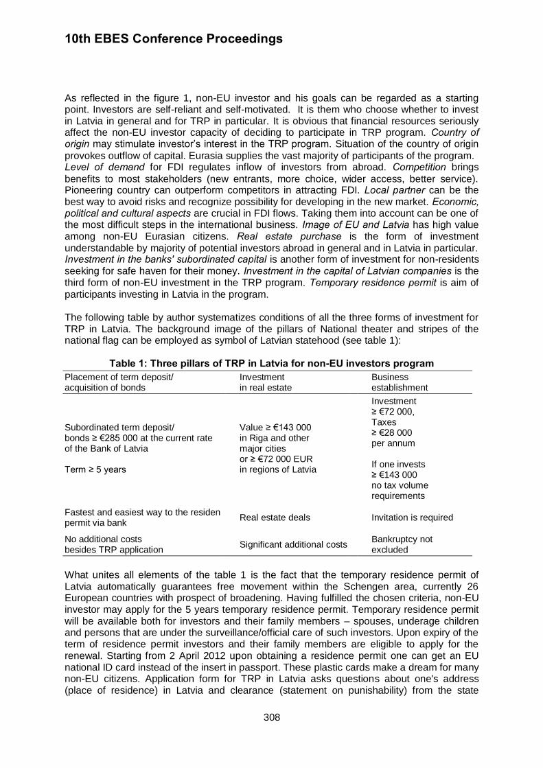
10th EBES Conference Proceedings
308
As reflected in the figure 1, non-EU investor and his goals can be regarded as a starting point. Investors are self-reliant and self-motivated. It is them who choose whether to invest in Latvia in general and for TRP in particular. It is obvious that financial resources seriously affect the non-EU investor capacity of deciding to participate in TRP program. Country of origin may stimulate investor’s interest in the TRP program. Situation of the country of origin
provokes outflow of capital. Eurasia supplies the vast majority of participants of the program. Level of demand for FDI regulates inflow of investors from abroad. Competition brings
benefits to most stakeholders (new entrants, more choice, wider access, better service). Pioneering country can outperform competitors in attracting FDI. Local partner can be the best way to avoid risks and recognize possibility for developing in the new market. Economic, political and cultural aspects are crucial in FDI flows. Taking them into account can be one of the most difficult steps in the international business. Image of EU and Latvia has high value among non-EU Eurasian citizens. Real estate purchase is the form of investment
understandable by majority of potential investors abroad in general and in Latvia in particular. Investment in the banks' subordinated capital is another form of investment for non-residents seeking for safe haven for their money. Investment in the capital of Latvian companies is the third form of non-EU investment in the TRP program. Temporary residence permit is aim of
participants investing in Latvia in the program. The following table by author systematizes conditions of all the three forms of investment for TRP in Latvia. The background image of the pillars of National theater and stripes of the national flag can be employed as symbol of Latvian statehood (see table 1):
Table 1: Three pillars of TRP in Latvia for non-EU investors program
Placement of term deposit/ acquisition of bonds
Investment in real estate
Business establishment
Subordinated term deposit/ bonds ≥ €285 000 at the current rate of the Bank of Latvia Term ≥ 5 years
Value ≥ €143 000 in Riga and other major cities or ≥ €72 000 EUR in regions of Latvia
Investment ≥ €72 000, Taxes ≥ €28 000 per annum If one invests ≥ €143 000 no tax volume requirements
Fastest and easiest way to the residence permit via bank
Real estate deals
Invitation is required
No additional costs besides TRP application
Significant additional costs Bankruptcy not excluded
What unites all elements of the table 1 is the fact that the temporary residence permit of Latvia automatically guarantees free movement within the Schengen area, currently 26 European countries with prospect of broadening. Having fulfilled the chosen criteria, non-EU investor may apply for the 5 years temporary residence permit. Temporary residence permit will be available both for investors and their family members – spouses, underage children and persons that are under the surveillance/official care of such investors. Upon expiry of the term of residence permit investors and their family members are eligible to apply for the renewal. Starting from 2 April 2012 upon obtaining a residence permit one can get an EU national ID card instead of the insert in passport. These plastic cards make a dream for many non-EU citizens. Application form for TRP in Latvia asks questions about one's address (place of residence) in Latvia and clearance (statement on punishability) from the state
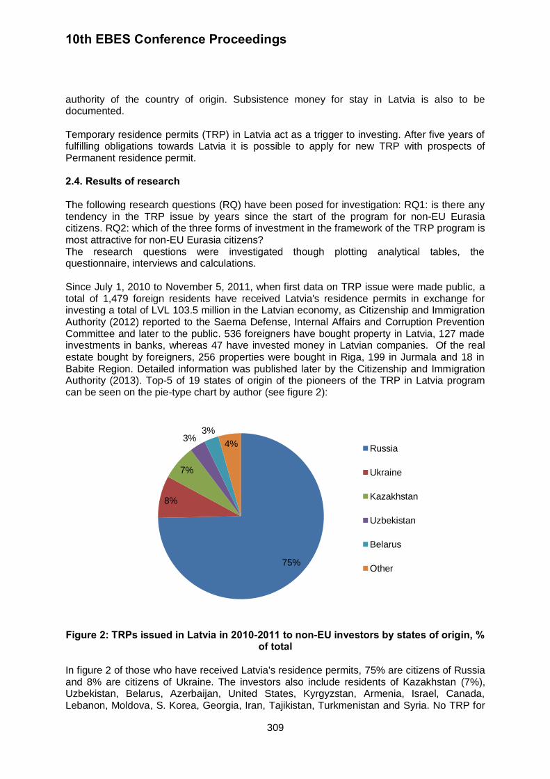
10th EBES Conference Proceedings
309
authority of the country of origin. Subsistence money for stay in Latvia is also to be documented. Temporary residence permits (TRP) in Latvia act as a trigger to investing. After five years of fulfilling obligations towards Latvia it is possible to apply for new TRP with prospects of Permanent residence permit. 2.4. Results of research The following research questions (RQ) have been posed for investigation: RQ1: is there any tendency in the TRP issue by years since the start of the program for non-EU Eurasia citizens. RQ2: which of the three forms of investment in the framework of the TRP program is most attractive for non-EU Eurasia citizens? The research questions were investigated though plotting analytical tables, the questionnaire, interviews and calculations. Since July 1, 2010 to November 5, 2011, when first data on TRP issue were made public, a total of 1,479 foreign residents have received Latvia's residence permits in exchange for investing a total of LVL 103.5 million in the Latvian economy, as Citizenship and Immigration Authority (2012) reported to the Saema Defense, Internal Affairs and Corruption Prevention Committee and later to the public. 536 foreigners have bought property in Latvia, 127 made investments in banks, whereas 47 have invested money in Latvian companies. Of the real estate bought by foreigners, 256 properties were bought in Riga, 199 in Jurmala and 18 in Babite Region. Detailed information was published later by the Citizenship and Immigration Authority (2013). Top-5 of 19 states of origin of the pioneers of the TRP in Latvia program can be seen on the pie-type chart by author (see figure 2):
Figure 2: TRPs issued in Latvia in 2010-2011 to non-EU investors by states of origin, % of total
In figure 2 of those who have received Latvia's residence permits, 75% are citizens of Russia and 8% are citizens of Ukraine. The investors also include residents of Kazakhstan (7%), Uzbekistan, Belarus, Azerbaijan, United States, Kyrgyzstan, Armenia, Israel, Canada, Lebanon, Moldova, S. Korea, Georgia, Iran, Tajikistan, Turkmenistan and Syria. No TRP for
75%
8%
7%
3% 3%
4% Russia
Ukraine
Kazakhstan
Uzbekistan
Belarus
Other
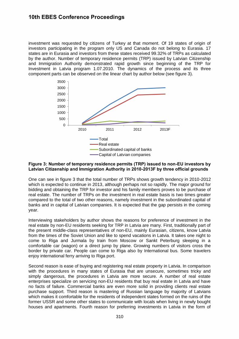
10th EBES Conference Proceedings
310
investment was requested by citizens of Turkey at that moment. Of 19 states of origin of investors participating in the program only US and Canada do not belong to Eurasia. 17 states are in Eurasia and investors from these states received 99.32% of TRPs as calculated by the author. Number of temporary residence permits (TRP) issued by Latvian Citizenship and Immigration Authority demonstrated rapid growth since beginning of the TRP for Investment in Latvia program 1.07.2010. The dynamics of the process and its three component parts can be observed on the linear chart by author below (see figure 3).
Figure 3: Number of temporary residence permits (TRP) issued to non-EU investors by Latvian Citizenship and Immigration Authority in 2010-2013F by three official grounds One can see in figure 3 that the total number of TRPs shows growth tendency in 2010-2012 which is expected to continue in 2013, although perhaps not so rapidly. The major ground for bidding and obtaining the TRP for investor and his family members proves to be purchase of real estate. The number of TRPs on the investment in real estate basis is two times greater compared to the total of two other reasons, namely investment in the subordinated capital of banks and in capital of Latvian companies. It is expected that the gap persists in the coming year. Interviewing stakeholders by author shows the reasons for preference of investment in the real estate by non-EU residents seeking for TRP in Latvia are many. First, traditionally part of the present middle-class representatives of non-EU, mainly Eurasian, citizens, know Latvia from the times of the Soviet Union and like to spend vacations in Latvia. It takes one night to come to Riga and Jurmala by train from Moscow or Sankt Peterburg sleeping in a comfortable car (wagon) or a direct jump by plane. Growing numbers of visitors cross the border by private car. People can come to Riga also by International bus. Some travelers enjoy international ferry arriving to Riga port. Second reason is ease of buying and registering real estate property in Latvia. In comparison with the procedures in many states of Eurasia that are unsecure, sometimes tricky and simply dangerous, the procedures in Latvia are more secure. A number of real estate enterprises specialize on servicing non-EU residents that buy real estate in Latvia and have no facts of failure. Commercial banks are even more solid in providing clients real estate purchase support. Third reason is mastering of Russian language by majority of Latvians which makes it comfortable for the residents of independent states formed on the ruins of the former USSR and some other states to communicate with locals when living in newly bought houses and apartments. Fourth reason for preferring investments in Latvia in the form of
0
500
1000
1500
2000
2500
3000
3500
2010 2011 2012 2013F
Total
Real estate
Subordinated capital of banks
Capital of Latvian companies
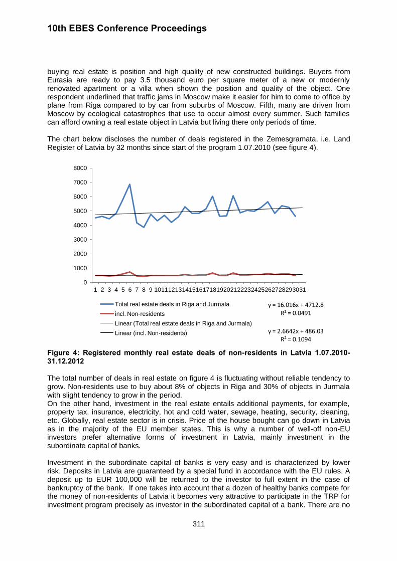
10th EBES Conference Proceedings
311
buying real estate is position and high quality of new constructed buildings. Buyers from Eurasia are ready to pay 3.5 thousand euro per square meter of a new or modernly renovated apartment or a villa when shown the position and quality of the object. One respondent underlined that traffic jams in Moscow make it easier for him to come to office by plane from Riga compared to by car from suburbs of Moscow. Fifth, many are driven from Moscow by ecological catastrophes that use to occur almost every summer. Such families can afford owning a real estate object in Latvia but living there only periods of time. The chart below discloses the number of deals registered in the Zemesgramata, i.e. Land Register of Latvia by 32 months since start of the program 1.07.2010 (see figure 4).
Figure 4: Registered monthly real estate deals of non-residents in Latvia 1.07.2010-31.12.2012 The total number of deals in real estate on figure 4 is fluctuating without reliable tendency to grow. Non-residents use to buy about 8% of objects in Riga and 30% of objects in Jurmala with slight tendency to grow in the period. On the other hand, investment in the real estate entails additional payments, for example, property tax, insurance, electricity, hot and cold water, sewage, heating, security, cleaning, etc. Globally, real estate sector is in crisis. Price of the house bought can go down in Latvia as in the majority of the EU member states. This is why a number of well-off non-EU investors prefer alternative forms of investment in Latvia, mainly investment in the subordinate capital of banks. Investment in the subordinate capital of banks is very easy and is characterized by lower risk. Deposits in Latvia are guaranteed by a special fund in accordance with the EU rules. A deposit up to EUR 100,000 will be returned to the investor to full extent in the case of bankruptcy of the bank. If one takes into account that a dozen of healthy banks compete for the money of non-residents of Latvia it becomes very attractive to participate in the TRP for investment program precisely as investor in the subordinated capital of a bank. There are no
y = 16.016x + 4712.8 R² = 0.0491
y = 2.6642x + 486.03 R² = 0.1094
0
1000
2000
3000
4000
5000
6000
7000
8000
1 2 3 4 5 6 7 8 9 10 11 12 13 14 15 16 17 18 19 20 21 22 23 24 25 26 27 28 29 30 31
Total real estate deals in Riga and Jurmala
incl. Non-residents
Linear (Total real estate deals in Riga and Jurmala)
Linear (incl. Non-residents)
10th EBES Conference Proceedings
312
additional costs in this investment. On the other hand, investment in the subordinated capital of a commercial bank in Latvia as elsewhere in the EU is subject to strict control in accordance with the money laundering prevention procedure. Investment demanded by Immigration Law is 200,000 Lats that is 284,474 euro, which is much above the guaranteed fund. Money is to be credited for five years. Both factors can detract potential investors from participation in the TRP for investment program. Already in December 2011 commercial bank AB according to Globenewswire (2011)1 exploited the opportunity by issuing subordinated bonds and later added two more issues. Rietumu bank followed suit according to Globenewswire (2012)2 and made one step forward by including subordinated bonds in the quotation list on OMX Baltic Stock Exchange. The importance of the above events is so big that deserves to be topic of special research. Last but not least opportunity to apply for TRP in Latvia is investment in the capital of enterprises. The tradition for non-EU investors to do business in Latvia is now deeply rooted. Investments from Eurasia giant, Russia, range Nr. 5 in the list of foreign direct investments (FDI) in Latvia by country of origin. The number of Joint ventures, where Latvian capital merges with Russian, is the leader in the international competition in Latvia. USA is investor Nr.11 and Ukraine Nr. 17. According to Lursoft (2013), in February 2013 non-EU investments in Latvia accumulate to almost 1 billion EUR, which constitutes 14.8% of the sum total. In terms of the number of enterprises, the non-EU investors make 49.7% of the sum total, namely 9955 enterprises. Non-EU investors appreciate belonging of Latvia to the EU and prospect of introduction of Euro in Latvia in 2014. Unfortunately the average size of non-EU investment in Latvian enterprise is rather small. It uses to be around EUR 100 000. The disproportion is due to the fact that EU investors use to invest huge sums in limited number of enterprises that are big by Latvian yardstick. It is important to investigate if the TRP for investment in Latvia program brings higher amounts of investment in the capital of enterprises in Latvia. The author has systematized statistics of investments done by applicants for TRP in Latvia. Analytical table by author is placed below (see table 2).
Table 2: Investments by applicants for TRP in Latvia in 2010-2013F (EURm) Non-EU investments, EURm, in:
2010 2011 2012 2013F SUM 2010-2012
Real estate 12.81 140.44 206.60 213.43 359.84
Subordinated capital of banks 6.26 41.41 28.17 28.46 75.84
Capital of Latvian companies 1.42 2.42 13.37 14.23 17.22
Total 20.49 184.26 248.15 256.12 452.90
It can be observed from the table 2 that the sum total of investments by non-EU applicants for TRP in 2012 has approached a quarter of a billion euro and cumulative by 1.01.2013 has approached half a billion euro. But compared to the internal non-financial investments in Latvia in 2012 (around EUR 3 billion) it is 8.3 %. The investments of non-EU TRP applicants in the capital of Latvian companies accumulated in the years 2010-2012 are to be compared to total accumulated non-financial foreign direct investments in Latvia (EUR 6,448,062,490)
1 AB bank to issue subordinated bonds. Available at:
<http://globenewswire.com/Tracker?data=bEJ7r_Co9l1aL8wDrR-WJbBuvcUtjD8Kn6cwHqqHtCIMwTg-KqRTJBPtRWS3xSUYZAlHz7kNrBtQpg_9hxvcb3aU4vKRm2XzeHvPs3x4EK4%3D>. 2 Rietumu bank to quote bonds. Available at: <http://globenewswire.com/news-
release/2012/12/06/509809/0/en/Rietumu-Banka-Will-List-Bonds-on-NASDAQ-OMX-Baltic-Market.html>.
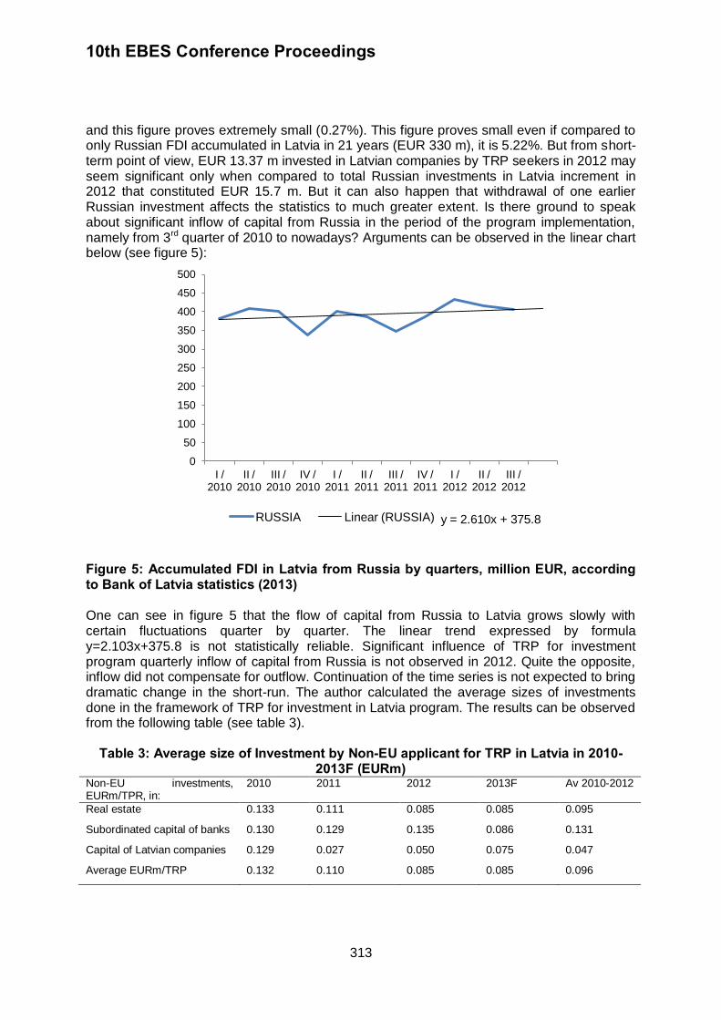
10th EBES Conference Proceedings
313
and this figure proves extremely small (0.27%). This figure proves small even if compared to only Russian FDI accumulated in Latvia in 21 years (EUR 330 m), it is 5.22%. But from short-term point of view, EUR 13.37 m invested in Latvian companies by TRP seekers in 2012 may seem significant only when compared to total Russian investments in Latvia increment in 2012 that constituted EUR 15.7 m. But it can also happen that withdrawal of one earlier Russian investment affects the statistics to much greater extent. Is there ground to speak about significant inflow of capital from Russia in the period of the program implementation, namely from 3rd quarter of 2010 to nowadays? Arguments can be observed in the linear chart below (see figure 5):
Figure 5: Accumulated FDI in Latvia from Russia by quarters, million EUR, according to Bank of Latvia statistics (2013) One can see in figure 5 that the flow of capital from Russia to Latvia grows slowly with certain fluctuations quarter by quarter. The linear trend expressed by formula y=2.103x+375.8 is not statistically reliable. Significant influence of TRP for investment program quarterly inflow of capital from Russia is not observed in 2012. Quite the opposite, inflow did not compensate for outflow. Continuation of the time series is not expected to bring dramatic change in the short-run. The author calculated the average sizes of investments done in the framework of TRP for investment in Latvia program. The results can be observed from the following table (see table 3).
Table 3: Average size of Investment by Non-EU applicant for TRP in Latvia in 2010-2013F (EURm)
Non-EU investments, EURm/TPR, in:
2010 2011 2012 2013F Av 2010-2012
Real estate 0.133 0.111 0.085 0.085 0.095
Subordinated capital of banks 0.130 0.129 0.135 0.086 0.131
Capital of Latvian companies 0.129 0.027 0.050 0.075 0.047
Average EURm/TRP 0.132 0.110 0.085 0.085 0.096
y = 2.610x + 375.8
0
50
100
150
200
250
300
350
400
450
500
I / 2010
II / 2010
III / 2010
IV / 2010
I / 2011
II / 2011
III / 2011
IV / 2011
I / 2012
II / 2012
III / 2012
RUSSIA Linear (RUSSIA)
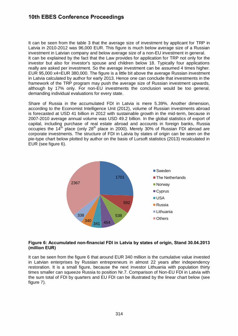
10th EBES Conference Proceedings
314
It can be seen from the table 3 that the average size of investment by applicant for TRP in Latvia in 2010-2012 was 96,000 EUR. This figure is much below average size of a Russian investment in Latvian company and below average size of a non-EU investment in general. It can be explained by the fact that the Law provides for application for TRP not only for the investor but also for investor's spouse and children below 18. Typically four applications really are asked per investment. So the average investment can be assumed 4 times higher. EUR 95,000 x4=EUR 380,000. The figure is a little bit above the average Russian investment in Latvia calculated by author for early 2013. Hence one can conclude that investments in the framework of the TRP program may push the average size of Russian investment upwards, although by 17% only. For non-EU investments the conclusion would be too general, demanding individual evaluations for every state. Share of Russia in the accumulated FDI in Latvia is mere 5.39%. Another dimension, according to the Economist Intelligence Unit (2012), volume of Russian investments abroad is forecasted at USD 41 billion in 2012 with sustainable growth in the mid-term, because in 2007-2010 average annual volume was USD 49.2 billion. In the global statistics of export of capital, including purchase of real estate abroad and accounts in foreign banks, Russia occupies the 14th place (only 28th place in 2000). Merely 30% of Russian FDI abroad are corporate investments. The structure of FDI in Latvia by states of origin can be seen on the pie-type chart below plotted by author on the basis of Lursoft statistics (2013) recalculated in EUR (see figure 6).
Figure 6: Accumulated non-financial FDI in Latvia by states of origin, Stand 30.04.2013 (million EUR)
It can be seen from the figure 6 that around EUR 340 million is the cumulative value invested in Latvian enterprises by Russian entrepreneurs in almost 22 years after independency restoration. It is a small figure, because the next investor Lithuania with population thirty times smaller can squeeze Russia to position Nr.7. Comparison of Non-EU FDI in Latvia with the sum total of FDI by quarters and EU FDI can be illustrated by the linear chart below (see figure 7).
1701
592
538
454 341 340
338
2367
Sweden
The Netherlands
Norway
Cyprus
USA
Russia
Lithuania
Others
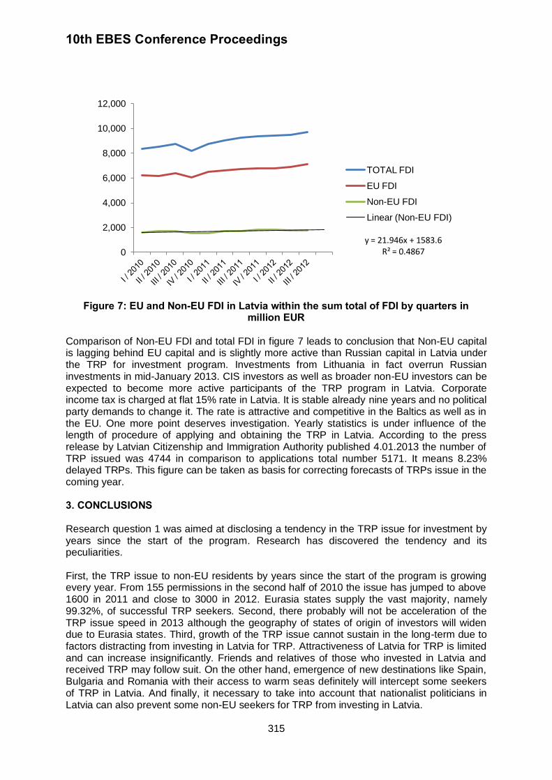
10th EBES Conference Proceedings
315
Figure 7: EU and Non-EU FDI in Latvia within the sum total of FDI by quarters in million EUR
Comparison of Non-EU FDI and total FDI in figure 7 leads to conclusion that Non-EU capital is lagging behind EU capital and is slightly more active than Russian capital in Latvia under the TRP for investment program. Investments from Lithuania in fact overrun Russian investments in mid-January 2013. CIS investors as well as broader non-EU investors can be expected to become more active participants of the TRP program in Latvia. Corporate income tax is charged at flat 15% rate in Latvia. It is stable already nine years and no political party demands to change it. The rate is attractive and competitive in the Baltics as well as in the EU. One more point deserves investigation. Yearly statistics is under influence of the length of procedure of applying and obtaining the TRP in Latvia. According to the press release by Latvian Citizenship and Immigration Authority published 4.01.2013 the number of TRP issued was 4744 in comparison to applications total number 5171. It means 8.23% delayed TRPs. This figure can be taken as basis for correcting forecasts of TRPs issue in the coming year. 3. CONCLUSIONS Research question 1 was aimed at disclosing a tendency in the TRP issue for investment by years since the start of the program. Research has discovered the tendency and its peculiarities. First, the TRP issue to non-EU residents by years since the start of the program is growing every year. From 155 permissions in the second half of 2010 the issue has jumped to above 1600 in 2011 and close to 3000 in 2012. Eurasia states supply the vast majority, namely 99.32%, of successful TRP seekers. Second, there probably will not be acceleration of the TRP issue speed in 2013 although the geography of states of origin of investors will widen due to Eurasia states. Third, growth of the TRP issue cannot sustain in the long-term due to factors distracting from investing in Latvia for TRP. Attractiveness of Latvia for TRP is limited and can increase insignificantly. Friends and relatives of those who invested in Latvia and received TRP may follow suit. On the other hand, emergence of new destinations like Spain, Bulgaria and Romania with their access to warm seas definitely will intercept some seekers of TRP in Latvia. And finally, it necessary to take into account that nationalist politicians in Latvia can also prevent some non-EU seekers for TRP from investing in Latvia.
y = 21.946x + 1583.6 R² = 0.4867 0
2,000
4,000
6,000
8,000
10,000
12,000
TOTAL FDI
EU FDI
Non-EU FDI
Linear (Non-EU FDI)
10th EBES Conference Proceedings
316
Research question 2 was aimed at comparing the three forms of investment in the framework of the TRP program for non-EU citizens. Research has disclosed that in the initial stage, real estate proves to be the most popular direction of investment. For lower middle class of non-EU states it is cheaper to apply for Schengen visas and finally get multi-visa for five years. But in the long run investment in the subordinated capital of banks will gain momentum. One can expect that non-EU investment in the capital of companies in Latvia will continue. This form of investment has own triggers and inertia and will go on mainly despite the TRP program. Latvia looks only a dot on the map for global non-EU investors. Those non-EU citizens who were ready to invest in the subordinate capital of banks are more interested in the guarantees of their deposits in Latvian banks. First, stability of the banking system is to be proven after scandalous crash of PAREX bank in 2008 and Latvijas Krajbanka in 2011. Second, strengthening of supervising body FCMC (FKTK) is a positive factor expected to make the system more transparent and predictable. Third, readiness of banks in Latvia for introduction of Basel III is a factor in favour of the future inflow of non-EU capital. According to the research, the sum total of investments by non-EU applicants for TRP in 2012 has approached a quarter of a billion euro. Compared to the internal non-financial investments in Latvia in 2012 it is 8.3 %. The figure can be introduced in the scientific circulation. The investments of TRP applicants in the capital of Latvian companies accumulated in the years 2010-2012 compared to total accumulated non-financial foreign direct investments in Latvia prove extremely small (0.000267%). This figure can grow with every next year of functioning of the program. But it is insignificant. Nevertheless compared to the last year non-EU FDI it becomes noticeable and can grow some time more in all three forms. One single form cannot be depicted as the most attractive. The hypothesis suggested in the beginning of research is proven. Residence Permits for Investment program in Latvia can be viable and successfully implemented in attraction of Eurasian investors. Directions for further research: Recipient States Attractiveness Index for Foreign Investors (RSAIFI), social portrait of non-EU TRP seeker from Eurasia, business incentives provided by Latvian state and EU funds, time series prolongation, case studies.
REFERENCES Amendments to the Immigration Law of 2002 (in Latvian Grozījumi Imigrācijas likumā 31.10.2002) in force 01.07.2010. 2010. Latvian Laws, [online] Available at:<
http://www.likumi.lv/doc.php?id=209646> [Accessed 9 January 2013] Baltic times, 2012. Latvia’s credit rating improves. [online] Available at:
<http://www.baltictimes.com/news/articles/32125/> [Accessed 14 January 2013]. Baltic times 2013. For love of money, sham marriages continue,.[online] Available at:
<http://www.baltictimes.com/news/articles/32417/> [Accessed 23 February 2013]. Bank of Latvia, 2013. FDI statistics. [online] Available at:
<http://statdb.bank.lv/lb/Data.aspx?id=104> [Accessed 10 April 2013]. Central statistical bureau CSB, 2013: Non-financial investments in Latvia in 2012 can breakthrough 2 bln LVL level (in Latvian). [online] Available at:
<http://www.csb.gov.lv/statistikas-temas/investicijas-galvenie-raditaji-30252.html> [Accessed 19 April 2013].
10th EBES Conference Proceedings
317
Citizenship and Immigration Authority, 2013. Press release (In Latvian) Foreigners invested above Ls 318 mln. [online] Available at:
<http://www.pmlp.gov.lv/lv/news/pazinojumi.html?news_id=853> [Accessed 4 January 2013]. Citizenship and Immigration Authority, 2012. TRP issue statistics for the first 18 months (in Latvian). [online] Available at: <http://www.pmlp.gov.lv/lv/statistika/uzturesanas.html>
[Accessed 5 February 2013]. Center for Global Development, 2012. The Commitment to development Index 2012, [online]
Available at: <http://www.cgdev.org/section/initiatives/_active/cdi/> [Accessed 11 March 2013]. The Economist Intelligence Unit, 2012. Report on perception of BRICs businessmen abroad, ordered by RUSAL, reviewed. [online] Available at: <http://lenta.ru/articles/2012/12/05/eiu/> [Accessed 16 January 2013]. The Economist, 2013. The Cyprus bail-out. Unfair, short-sighted and self-defeating. [online]
Available at: <http://www.economist.com/blogs/schumpeter/2013/03/cyprus-bail-out> [Accessed 17 March 2013]. Economist Intelligence Unit, 2007. World investment prospects to 2011. Foreign direct investment and the challenge of political risk. London: Economist Intelligence Unit.
Index of economic freedom, 2013 (by Heritage Foundation in partnership with Wall Street
Journal). [online] Available at: <http://www.heritage.org/index/> [Accessed 22 April 2013].
Francis, J. and Ibbotson, R., 2002. Investments A Global Perspective. New Jersey: Prentice Hall . Gregor, A., 2012 International real estate: House hunting in…Latvia. [online] Available
at:<http://www.nytimes.com/2012/04/04/greathomesanddestinations/real-estate-in-latvia.html?pagewanted=all&_r=3&> [Accessed 5 April 2013]. Hill, C.W.L., 2009. International Business. 7th ed. McGraw-Hill/Irwin. Krugman, P., 2013. The Conscience of a Liberal. [online] Available at:
<http://krugman.blogs.nytimes.com/2013/05/01/baltic-brouhaha/?_r=0> [Accessed 1 May 2013] Pavluts, D., 2012 Russia-Latvia International conference Cooperation in Economics. [online]
Available at: <http://konferences.db.lv/arhivs/latvijas-un-krievijas-ekonomiska-sadarbiba/> [Accessed 9 April 2013]. Real Estate Nira Fonds, 2013 [online] Available at: <https://rus.db.lv/nedvizhimost/nira-fonds-v-rige-za-iv-kvartal-lish-8-proc-sdelok-zakljucheno s ner4ezidentami-50142> [Accessed 5 February 2013] . Schwab, C., 2012. The Global Competitiveness Report 2012-2013. World Economic Forum,
Geneva: WEF Sekaran, U., 2003. Research methods for business. 4th ed. New York: John Wiley and Sons.

10th EBES Conference Proceedings
318
Three Latvian Companies headed by Baltic Sotheby's International Realty research, 2012. Profile of foreign investor. [online] Available at: <http://rus.db.lv/nedvizhimost/portret-
inostranca-investora-s-vnzh-zhenat-molod-obrazovan-i-uspeshen-48137?cp=1> [Accessed 11 January 2013]. Wheatley, A. and Tapinsh, A., 2013. Analysis - Resilient Latvia ready for euro but reforms needed. [online] Available at: <http://uk.reuters.com/article/2013/03/12/uk-eurozone-latvia-
prospects-idUKBRE92B0HC20130312> [Accessed 13 March 2013].
10th EBES Conference Proceedings 23 - 25 May, 2013. NIPPON HOTEL, ISTANBUL, TURKEY ISBN: 978-605-64002-1-6. WEBSITE: www.ebesweb.org
319
A STUDY ON STAKEHOLDER MODEL CHANGE AND SOCIAL RESPONSIBILITY TYPE FOR FOXCONN IN CHINA
BYUNG HUN CHOI
Business Administration Department Kongju National University
South Korea [email protected]
Abstract: Foxconn, the biggest electrical manufacturing service provider in global consumer
electronics, tries to change after employees’ suicide accidents in China. The change mostly goes toward the recovery of employees’ interest. As of May 2013 Foxconn has successfully completed the remedial tasks that recommended by FLA. Accordingly this study considered such a change as a restoration process for employees’ benefit that had been infringed by other stakeholders, customer and local government. In addition there had been a recognition gap between Foxconn and third-party evaluators regarding corporate social responsibility (CSR) activities of Foxconn, so this study clarified it through FLA investigation report and GRI guideline version 3.1. As a result it turned out that CSR type of Foxconn rarely go beyond the responsive CSR range although it has improved the working conditions after FLA investigation. Keywords: Foxconn, Foxconn Employee Suicide, CSR (Corporate Social Responsibility) of
Foxconn, Hon Hai, Stakeholder Model 1. INTRODUCTION In recent Foxconn (Fushikang) has been taken a big notice in the world. The reason would
be sum up with two points; firstly, it is a core partner of Apple in making iPod, iPhone, iPad, and secondly twenty young workers committed suicide at Foxconn factories in China from January 2010 to December 2011. Lots of media reported that there were sufferings and tears of Chinese migrant workers behind a great performance of Apple. Accordingly the successive suicide accidents in Foxconn made Apple and FLA (Fair Labor Association)1 directly investigate the working conditions for Foxconn three factories in China.2 As a result, FLA found at least 50 issues that seriously violated not only FLA’s Workplace Code of Conduct but also Chinese labor law (FLA, 2012a). After the FLA investigation, Foxconn and Apple prepared the remedial measures to address each issue pointed out by FLA. Furthermore it turned out that most of remedial actions were completed smoothly as it scheduled for a period of 15 months from April 2012 to July 2013 (FLA, 2012b). So it can be said that there are some changes at the Foxconn's policy for local employees' welfare. But it needs more time to judge the sustainability of such changes because business environment change of global IT industry can cause another turnover on the value chain of Foxconn in future (Chan, 2011). However it surely works as a meaningful momentum for the turnover of Foxonn’s CSR (Corporate Social Responsibility) activity. When considering that
1 Fair Labor Association (FLA) is a collaborative effort of universities, civil society organizations and socially
responsible companies dedicated to protecting workers’ rights around the world. It is an international non government organization (NGO), and headquartered in Washington, D.C., with offices in China, Switzerland and Turkey. 2 After suicide accidents happened in Foxconn factories, Apple agreed to allow FLA to conduct a thorough
investigation for three factories at Guanlan(February 14-17), Longhua(March 5-8), Chengdu(March 6-9) in early 2012 (FLA, 2012a).
10th EBES Conference Proceedings
320
CSR is a direct or indirect responsibility for whole members in local community, the objects of CSR activity can be summarized as six representative members who have some concern in a firm’s business, so called stakeholders; customer, employee, competitor, supplier(collaborating firm), investor(shareholder), local community or state (Choi, 2008). If a firm prefers the stakeholder model to shareholder's value maximization model, it means that the firm takes a more balanced approach for those six stakeholders’ interests rather than firstly considers shareholder’s interest (Jeong, 2006). Further at the point of stakeholder model view, the recent change of Foxonn for improving employees' welfare can be depicted as a recovering process of employees’ interests that infringed by other stakeholders. This study intends to access the working condition for Chinese local employees of Foxconn with assuming that Foxconn and FLA took the different approaches for local employees' welfare. It can be explained as a recognition gap between Foxconn and third-party evaluators. In addition the main issues of this study are as follows; firstly what is the difference between Foxconn and FLA for the working condition of local employees in China? Also how can evaluate the overall CSR condition of Foxconn through the GRI (Global Reporting Initiative)3 guideline version 3.1? Secondly what is the meaning for the remedial actions of Foxconn at the viewpoint of stakeholder model change? Especially this study tried to clarify the recovering process by centering on the relation change among three stakeholders; employee, customer, local government or community. Thirdly how can analyze the working condition reform at the viewpoint of CSR type, and what is the implication for other firms operated in China? At the next chapter this study reviewed theoretical background for CSR and stakeholder model, and suggested research method. Previous studies for Foxconn and the employees' suicide accidents were also examined. At chapter three this study analyzed the recognition gap between Foxconn and third-party evaluators, FLA and GRI. At chapter four, this study tried to suggest a significance of the relation change among three stakeholders after FLA investigation, and discussed the CSR type of Foxconn.
2. PREVIOUS STUDIES AND THEORETICAL BACKGROUND 2.1. Previous studies
The topics of previous studies regarding Foxconn can be largely grouped into two issues; the success factor analysis for its business model, and cause & effect analysis for employees' suicide accidents. Ngai and Chan (2012) handled Foxconn’s growth as an expansion process of monopoly capital, and looked into its impact on frontline workers’ lives in China. They also clarified the involvement of Chinese government in facilitating Foxconn’s capital expansion in whole area of China, and explored what made production line workers conduct suicides through the field survey and personal interviews for workers. In particular Su (2011) concentrated on student workers (xueshenggong) issue of Foxconn, and reviewed the
mechanism engaged in the mutually complementary commodification of education and labor. With taking the institutional approach for Chinese unique student intern system, Su argued that Chinese state played a critical role in forming the exchange pattern between technical schools and Foxconn.
3 This study selected the GRI (Global Reporting Initiative) as another third-party evaluator for Foxconn CSR
activities and reviewed Foxconn CSR report by using the articles of GRI guideline version 3.1. GRI is a multi-stakeholders, global network based non-profit organization that established in 1997. It works for a sustainable global economy by providing sustainability reporting guideline and has made a close partnership with UNEP, UN Global Compact and ISO to realize its goal.
10th EBES Conference Proceedings
321
Guo et al. (2012) tried to draw out the difference of international perspectives to Foxconn employees’ suicides through the quantitative & qualitative approach for 92 newspapers in United States and China. As a result they turned out that Chinese newspaper framed the suicide cases mainly as psychological problems of a young generation rather than a sweatshop style management of Foxconn. They also suggested other three perspectives regarding Foxconn suicides; economic consequence for local community development, global consumption vs. production, global labor vs. capital. Umlas (2012) insisted that big global firms like Apple, HP or Sony should take more responsibility for employees’ welfare of suppliers by directly investigating labor contracts or working environment of suppliers’ local factories. However Rulliat (2010) emphasized not only the lack of social responsibility of Foxconn but also the lack of education and the weak psychological strength of some workers as a reason for suicide accidents. Deffree (2011) argued that Apple has to do more assignments than Foxconn in order to accomplish the CSR goal for Chinese local workers. On the other hand, Jang (2012) made an analysis for key success factors of Foxconn at the point of corporate strategy view, and presented three factors. Kam (2010) followed up the strategy transformation tendency of global contract manufacturing business for consumer electronics while looking into the partnership between Apple and Foxconn. 2.2. Theoretical background The concept of CSR is so broad as to be hardly defined by a simple sentence because the social responsibility (SR) of a firm has been different by every region or country (Jang and Seok, 2007; Choi, 2008). Traditionally UN has put an emphasis on three factors; environment, society, governance, what is called the ESG model regarding CSR activity (Choi and We, 2008). Bowen (1953) defined CSR as a sort of obligation to do something, to follow the rule, and to make a decision which is desirable to the object and value of society (Kim et al., 2005). Recently many global firms have considered GRI guidelines4 as a global
standard for CSR activities and CSR reporting (Porter and Kramer, 2006). This study also took a deep interest in the GRI because GRI regards CSR as the organization’s balanced approach for economy, society and environment issues, so called Triple Bottom Line (Kwak, 2006). In March 2011, GRI suggested the guideline version 3.1, so call the G3.1 that a new version for G3 guideline announced in 2006, and the G3.1 became a mostly applied sustainable reporting framework all over the world.5 The G3.1 consists of 124 articles, and two major parts of it are the profile disclosures(40 articles) and the performance indicators(84 articles). The profile disclosures cover four sections; the strategy & analysis, the organizational profile, the report parameters, and the governance, commitments & engagement (GRI, 2011). In addition, The performance indicators are organized by economic(9 articles), environmental(30 articles) and social(45 articles) indicators. More specifically the social indicators are grouped into four categories; the labor(15 articles), human rights(11 articles), local society(10 articles), product responsibility(9 articles).
4 Actually GRI guidelines have a goal to induce a firm's voluntary reporting about its CSR activities rather than the
mandatory assignment. But in order to take the application level check for the CSR activities, every firm should make CSR report conform with the GRI guidelines(G3.0 or G3.1) and publish the check list result between the guideline and CSR report (Ha, 2011). 5 G3.1 mostly takes a same stance as existing G3 but G3.1 increased performance indicators, upgraded the
measurability for CSR activities as well as required a firm open the negative information for it (Ha, 2011).
10th EBES Conference Proceedings
322
However since late 1990s the focus of academic discussion for CSR has laid on stakeholder6 model rather than shareholder value maximization. In order for a sustainable development it became much more important for a firm to consider not only shareholder’s position but also other stakeholders’ interests (Kabu, 1997; Martin, 2002). Especially Martin (2010, 61) argued many evidences supported that shareholder top priority policy rarely contributed to the value increase for shareholders because of only concentrating on a short term trade-off for their stocks without looking at each firm’s fundamental capability. Further He emphasized that making customer value a top priority would create shareholder return in the long run (Martin, 2010). Generally the representative stakeholders of a firm include six objects; customer, employee, competitor, supplier, investor, local community or state (Jeong, 2006). Regarding the CSR type, Porter and Kramer (2002, 60) presented a new way to create a competitive advantage through four elements of diamond model; context for strategy and rivalry, factor conditions, demand conditions, related & supporting industries. They defined a common space that firm philanthropy, a social benefit, and shareholder interests, the economic gains converges as a ‘convergence of interests’ (Porter and Kramer, 2002). After then they also suggested that a firm should integrate a firm’s success and social welfare while mitigating the conflicts between business and society (Porter and Kramer, 2006). On the basis of a firm’s prioritizing activity as for three types of social issues; generic social issues, value chain social impacts, social dimensions of competitive context, they classified CSR activity into two types; responsive CSR and strategic CSR (Porter and Kramer, 2006). The responsive CSR comprises two factors: acting as a good corporate citizen, attuned to evolving social concerns of stakeholder, and mitigating current or anticipated adverse effects of business activities (Porter and Kramer, 2006). On the other hand, the strategic CSR moves beyond a good corporate citizenship and mitigating harmful value chain impacts. It means value chain change to benefit society as well as strategic philanthropy that leverages capabilities to improve salient area of competitive context (Porter and Kramer, 2006). By taking a similar approach for the relation between social welfare and business profit, Choi (2008) also classified CSR activity into three types; preventive CSR, responsive CSR, strategic CSR. Recently Porter and Kramer (2011) presented a new idea for CSR, so called CSV(Creating Shared Value) which defined as policies or operating practices that enhance the competitiveness of a company while simultaneously advancing the business and social conditions at each community. They argued the significance of interaction or goal sharing between firms and governments or NGOs, therefore CSV should supersede CSR in guiding overall business activities and in creating the competitive advantage for a firm (Porter and Kramer, 2011). 2.3. Research method
As mentioned at the chapter one, this study accessed both overall CSR activity of Foxconn and the working condition with assuming that Foxconn and third-party evaluators had different opinions. This study applied FLA's reports as well as GRI guideline version 3.1(G3.1) to evaluate the CSR activities and the working condition. Firstly this study analyzed the Foxconn CSER (Corporate Social and Environmental Responsibility) report published in June 2011 by using GRI G3.1 indicators to evaluate the overall CSR condition. Basically this study assumed that each firm's CSR activities are mostly reflected in its own CSR report although it tends to just release the positive side of them. In particular this study examined
6 The stakeholder of a firm means the person, party, organization that a firm cannot make a business without its
consent or support (Jeong, 2006; Choi, 2008).
10th EBES Conference Proceedings
323
how many articles of G3.1 indicators were included in Foxconn CSER report, which articles were excluded, and looked into the reason. Secondly this study reviewed the FLA investigation report published in March 2012 and the verification status report released in August 2012 to access the working condition of Foxconn. This study picked out three issues regarding working condition of Foxconn on the basis of FLA reports. In fact the FLA investigation had been done by a request of Apple, so FLA’s inspectors directly visited three factories of Foxconn that located at Guanlan and Longhua in Shenzhen city, and in Chengdu city from February to March in 2012. After the investigation, FLA published detailed reports for three factories and suggested recommendations to address the related issues. Apple and Foxconn presented a complete remediation plan to address the issues, and the action plan is scheduled to be done for next 15 months, from April 2012 to July 2013. Thirdly this study tried to draw out the meaning of working condition reform after FLA investigation. This study summarized the main contents of working condition reform as four points, and analyzed them from the viewpoint of interest relation change among stakeholders of Foxconn. In addition this study analyzed the CSR type of Foxconn according to the theoretical review for the responsive CSR and the strategic CSR. Consequently this study can be differentiated from previous studies as next three points. Firstly this study introduced GRI G3.1 checklist to evaluate the overall CSR activities of Foxconn as well as to analyze the CSR type for the first time. Further this study tried to acquire the objective data for the working condition of Foxconn through the FLA reports. Such trials can be interpreted as a collaborating process with applying various NGOs' researches at the academic field. In particular this study will be helpful for the future studies regarding CSR or labor issue in making the research plan. Secondly, this study applied previous theories regarding CSR type and stakeholder model as much as possible to explain the suicide accidents at the point of academic view. On the contrary other previous studies mainly focused on clarifying the poor working condition of Foxconn, and tried to connect it with the suicide accidents. In fact FLA also took a similar approach as them. And other studies reviewed the key success factors at the viewpoint of unique business model of Foxconn. Therefore this study will be able to contribute to the application of CSR type theory as well as the development of stakeholder model. Finally this study can present a fresh perspective for global companies in China, because it would be very useful for them to clearly understand the recent trend for employment contract and local employees' welfare. Recently China lies in a turnover period for the existing world factory's role due to the labor cost increase. In order to expand the practical implication for business, this study suggested three points regarding the labor issue of China at conclusion part. 3. INTERNAL AND THIRD-PARTY EVALUATION ON CSR ACTIVITY of FOXCONN: A CRITICAL COMPARISON
3.1. Evaluation for overall CSR activity by GRI G3.1 Hon Hai Precision Industry Company Ltd., the anchor company of a globally well known name, Foxconn, was founded in Taipei in 1974. In 2011 its revenue reached 92 billion US dollar, and the CAGR of revenue for recent ten years since 2001 was 36%. Foxconn also took 60th in 2011 among Fortune 500 biggest companies while greatly jumping from the
raking of previous year, 112th (Ngai and Chan, 2012). In particular it took 5th place for IT firm listing following Samsung Electronics(22nd), HP(28th), Panasonic(50th), IBM(52nd) (Jang, 2012). At the global electronics manufacturing service (EMS), Foxconn’s market share was
10th EBES Conference Proceedings
324
just 3% in 2001 but it went up to 22% in 2005, and reached 44%, 50% in 2010 and in 2011 respectively (Jang, 2012).Especially such a rapid leap during recent 3~4 years is closely concerned with a strong partnership between Foxconn and Apple. The proportion of Apple’s products for whole revenue of Foxconn went up to 45% by the first quarter of 2012, from 26% in 2010, 33% in 2011 respectively (Jang, 2012). In addition Foxconn was able to possess more than 60% of total orders of Apple as an exclusive provider role for iPhone and iPad (Kam, 2010; Hermanson, 2011). By 2011 total number of Foxconn employees went over one million, and the CAGR of it from 2001 to 2011 reached 35.8% (Foxconn Technology Group, 2012). However over 90% of them were hired at the mainland China. Internally Foxconn has published the overall CSR activities through annual report, so called the ‘Stakeholder Management,’ which follows a general stakeholder model (Table 1). Top management including CEO, Terry Guo (Guo,TaiMing) considers its stakeholders as six
objects; investor, employee, customer, supplier, community, NGOs (Foxconn Technology Group, 2011). The CSR activities for employees focus on the working & living condition improvement, social network, labor relation and mental health care program. After a series of employee suicide accidents, Foxconn tries to communicate with employees for timely knowing their emotional depression or hardship. The communication channels include 24 hour hotline, regular forum, letter box, job satisfaction survey, mental counseling (Foxconn Technology Group, 2011). However the CSR activities for customers focus on global IT firms rather than general people because the main business of Foxconn is to manufacture IT products by their orders. Above all both the flexible manufacturing system and swift response ability to the changeable orders make a big contribution for Foxconn to be a competitive partner (Su, 2011; Ngai and Chan, 2012; Smith, 2011). As the third-party evaluation this study analyzed the report by GRI G3.1 to review how much its CSR activities agree with the global standard. In result the report included all of the articles in profile disclosure part of G3.1 but the coverage rate for 84 articles in performance indicators part was only 44%.
In detail it can be summarized as (Table 2-1), (Table 2-2), (Table 2-3) and (Table 2-4). Among nine articles of ‘Economic Performance (EC)' section, seven articles except EC5, EC9 were covered by the report(Table 2-1), and the coverage rate reached 77.8%. However at ‘Environment Performance (EN)’ section just 11 articles among 30 were mentioned in the report (Table 2-1)~(Table 2-2), and the coverage rate was 36.7%. The report rarely covered ‘Biodiversity,’ ‘Emissions, Effluents & Waste,’ ‘Products & Services,’ ‘Compliances,’ ‘Transport’ articles. It might be closely concerned with the actual role of Foxconn as a manufacturing service provider rather than a global maker having its own brand equity (Hermanson, 2011).

10th EBES Conference Proceedings
325
Table 1: Overall CSR activity of Foxconn: Stakeholder management model
Stakeholders Communication
Methods Key
Assignments Major Activities
Employees
Regular employee forum, letter box, job satisfaction survey, 24-hour hotline, mental health program & counseling system, employee assistant funds
Working & living condition upgrade, employees' social relation guarantee, mental health care service
To keep track of workers' voices & requests. To find out workers who got emotional depression & to make a timely counseling system is very critical.
Customers
Customers' randum visits & audits, quarterly & annual audits, telephone conference, SER-in Action conference
Green products, energy saving & carbon footprint, EICC Code of Conduct application
To provide customers with fast, innovative, flexible, cost saving manufacturing services. To keep effective communication channels to make a swift response for buyers' changeable orders.
Suppliers
Irregular SER audits, annual suppliers' meeting for SER audits
Inspect supplies' EICC CoC & CSR activities
To request suppliers keep Foxconn SER standards by annual supplies' meeting, unscheduled SER audits.
Community
Sustainable & continuous (monthly, quarterly, annual) charity activities
Ecosystem preserve program, financial aid program for the poor, children & juvenile education in local community
To improve energy saving, emission reduction, green energy, recycling effect at value chain. Employees are required to contribute their capabilities for environment preserve, the poor assistant.
Investors
Annual offline meeting for stockholders, investor phone conference, financial reports(monthly, quarterly, annually) release
Overall business condition, financial performance, SER observance update
To provide investors with a peace of mind, timely information for business condition. To get investors' trust through transparency
NGOs
Unscheduled telephone conferences, continuous online & offline meeting
Employee welfare, environment care & conservation
To get annual SER forums & collaborate with various NGOs for SER projects.
Sources: Foxconn 2011 CSER Annual Report, p.9; Foxconn 2010 CSER Annual Report, p.11.

10th EBES Conference Proceedings
326
Table 2-1: GRI G3.1 performance indicators analysis for Foxconn 2011 CSER report Aspect Description Report Section
Economic Performance Indicators
Economic Performance
EC1 Direct economic value generated & distributed, including revenues, operating cost, employee compensation, donations & other community investments, retained earnings, payment to capital providers & governments
1.1/4.1/4.2/4.3
EC2 Financial implications & other risks & opportunities for the organization's activities due to climate change.
5.1
EC3 Coverage of the organization's defined benefit plan obligations. 2.2
EC4 Significant financial assistance received from government. 1.2
Market Presence
EC5 Range of ratios of standard entry level wage by gender compared to local minimum wage at significant locations of operation.
None
EC6 Policy, practices & proportion of spending on locally based suppliers at significant locations of operation.
6/6.1
EC7 Procedures for local hiring & proportion of senior management hired from the local community at significant locations of
operation.
2.1
Indirect Economic Impacts
EC8 Development & impact of infrastructure investments & services provided primarily for public benefit through commercial, in-kind, or pro bono engagement.
4.1/4.2/4.3
EC9 Understanding & describing significant indirect economic impacts, including the extent of impacts.
None
Environment Performance Indicators
Materials EN1 Materials used by weight or volume. None EN2 Percentage of materials used that are recycled input materials. 5.2
Energy
EN3 Direct energy consumption by primary energy source. None EN4 Indirect energy consumption by primary source. 5.1
EN5 Energy saved due to conservation & efficiency improvements. 5.1
EN6 Initiatives to provide energy-efficient or renewal energy based products & services, & reductions in energy requirements as a result of these initiatives.
None
EN7 Initiative to reduce indirect energy consumption & reductions achieved.
5.1
Water
EN8 Total water withdrawal by source. 5.3
EN9 Water sources significantly affected by withdrawal of water. None EN10 Percentage & total volume of water recycled & reused. 5.3
Biodiversity
EN11 Location & size of land owned, leased, managed in, or adjacent to, protected areas & areas of high biodiversity value outside protected areas.
None
EN12 Description of significant impacts of activities, products, & services on biodiversity in protected areas & areas of high biodiversity value outside protected areas.
None
EN13 Habitats protected or restored. None EN14 Strategies, current actions, & future plans for managing impacts
on biodiversity. None
EN15 Number of IUCN Red List species & national conservation list species with habitats in areas affected by operations, by level of
extinction risk.
None
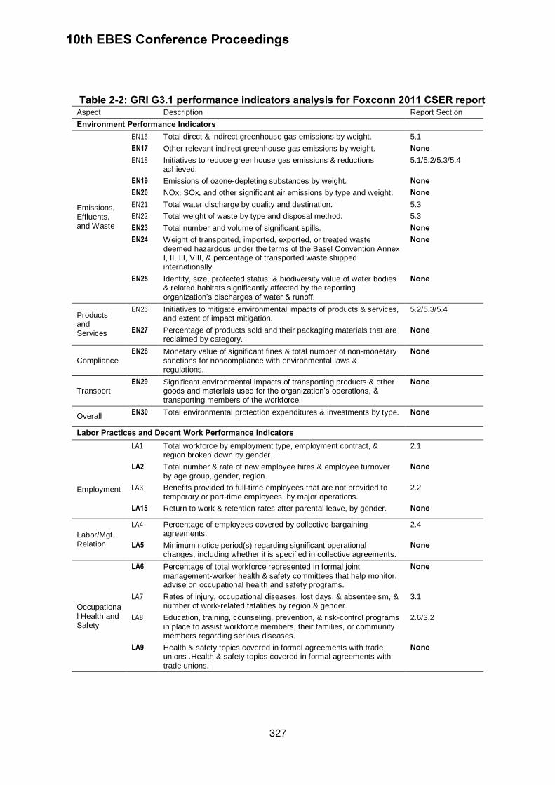
10th EBES Conference Proceedings
327
Table 2-2: GRI G3.1 performance indicators analysis for Foxconn 2011 CSER report Aspect Description Report Section
Environment Performance Indicators
Emissions, Effluents, and Waste
EN16 Total direct & indirect greenhouse gas emissions by weight. 5.1
EN17 Other relevant indirect greenhouse gas emissions by weight. None EN18 Initiatives to reduce greenhouse gas emissions & reductions
achieved. 5.1/5.2/5.3/5.4
EN19 Emissions of ozone-depleting substances by weight. None EN20 NOx, SOx, and other significant air emissions by type and weight. None EN21 Total water discharge by quality and destination. 5.3
EN22 Total weight of waste by type and disposal method. 5.3
EN23 Total number and volume of significant spills. None EN24 Weight of transported, imported, exported, or treated waste
deemed hazardous under the terms of the Basel Convention Annex I, II, III, VIII, & percentage of transported waste shipped internationally.
None
EN25 Identity, size, protected status, & biodiversity value of water bodies & related habitats significantly affected by the reporting organization’s discharges of water & runoff.
None
Products and Services
EN26 Initiatives to mitigate environmental impacts of products & services, and extent of impact mitigation.
5.2/5.3/5.4
EN27 Percentage of products sold and their packaging materials that are reclaimed by category.
None
Compliance
EN28 Monetary value of significant fines & total number of non-monetary sanctions for noncompliance with environmental laws & regulations.
None
Transport EN29 Significant environmental impacts of transporting products & other
goods and materials used for the organization’s operations, & transporting members of the workforce.
None
Overall EN30 Total environmental protection expenditures & investments by type. None
Labor Practices and Decent Work Performance Indicators
LA1 Total workforce by employment type, employment contract, &
region broken down by gender. 2.1
Employment
LA2 Total number & rate of new employee hires & employee turnover by age group, gender, region.
None
LA3 Benefits provided to full-time employees that are not provided to temporary or part-time employees, by major operations.
2.2
LA15 Return to work & retention rates after parental leave, by gender. None
Labor/Mgt.
Relation
LA4 Percentage of employees covered by collective bargaining agreements.
2.4
LA5 Minimum notice period(s) regarding significant operational changes, including whether it is specified in collective agreements.
None
Occupational Health and
Safety
LA6 Percentage of total workforce represented in formal joint management-worker health & safety committees that help monitor, advise on occupational health and safety programs.
None
LA7 Rates of injury, occupational diseases, lost days, & absenteeism, & number of work-related fatalities by region & gender.
3.1
LA8 Education, training, counseling, prevention, & risk-control programs
in place to assist workforce members, their families, or community members regarding serious diseases.
2.6/3.2
LA9 Health & safety topics covered in formal agreements with trade unions .Health & safety topics covered in formal agreements with trade unions.
None

10th EBES Conference Proceedings
328
Table 2-3: GRI G3.1 performance indicators analysis for Foxconn 2011 CSER report Aspect Description Report Section
Labor Practices and Decent Work Performance Indicators
Training and Education
LA10 Average hours of training per year per employee by gender & by employee category.
2.6
LA11 Programs for skills management and lifelong learning that support the continued employability of employees and assist them in managing career endings.
2.6
LA12 Percentage of employees receiving regular performance & career development reviews by gender.
2.6
Diversity and Equal Opportunity
LA13
Composition of governance bodies & breakdown of employees per employee category according to gender, age group, minority group membership, & other indicators of diversity.
2.1
Equal Remuneration for Women and Men
LA14 Ratio of basic salary & remuneration of women to men by employee category, by significant locations of operation.
None
Human Rights Performance Indicators
Investment and Procurement Practices
HR1 Percentage & total number of significant investment agreements & contracts that include clauses incorporating human rights concerns, or that have undergone human rights screening.
None
HR2 Percentage of significant suppliers, contractors, & other business partners that have undergone human rights screening, & actions taken.
None
HR3 Total hours of employee training on policies & procedures concerning aspects of human rights that are relevant to operations, including the percentage of employees trained.
1.2/2.6
Non-discrimination
HR4 Total number of incidents of discrimination & corrective actions taken.
None
Freedom of Association & Collective Bargaining
HR5
Operations & significant suppliers identified in which the right to exercise freedom of association & collective bargaining may be violated or at significant risk, & actions taken to support these rights.
2.4
Child Labor HR6 Operations & significant suppliers identified as having significant risk for incidents of child labor, & measures taken to contribute to the effective abolition of child labor.
2.1/6.1
Force and Compulsory Labor
HR7
Operations & significant suppliers identified as having significant risk for incidents of forced or compulsory labor, & measures to contribute to the elimination of all forms of forced or compulsory labor.
2.1/6.1
Security Practices
HR8 Percentage of security personnel trained in the organization’s policies or procedures concerning aspects of human rights that are relevant to operations.
None
Indigenous Rights
HR9 Total number of incidents of violations involving rights of indigenous people and actions taken.
None
Assessment HR10 Percentage & total number of operations that have been subject to human rights reviews and/or impact assessments.
None
Remediation HR11 Number of grievances related to human rights filed, addressed, & resolved through formal grievance mechanisms.
2.4
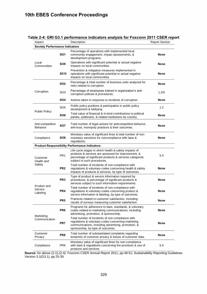
10th EBES Conference Proceedings
329
Table 2-4: GRI G3.1 performance indicators analysis for Foxconn 2011 CSER report Aspect Description Report Section
Society Performance Indicators
Local Communities
SO1 Percentage of operations with implemented local community engagement, impact assessments, & development programs.
None
SO9 Operations with significant potential or actual negative impacts on local communities.
None
SO10 Prevention & mitigation measures implemented in operations with significant potential or actual negative
impacts on local communities.
None
Corruption
SO2 Percentage & total number of business units analyzed for risks related to corruption.
None
SO3 Percentage of employees trained in organization’s anti-corruption policies & procedures.
1.2/6
SO4 Actions taken in response to incidents of corruption. None
Public Policy
SO5 Public policy positions & participation in public policy
development & lobbying. 1.2
SO6 Total value of financial & in-kind contributions to political parties, politicians, & related institutions by country.
None
Anti-competitive Behavior
SO7 Total number of legal actions for anticompetitive behavior, anti-trust, monopoly practices & their outcomes.
None
Compliance SO8 Monetary value of significant fines & total number of non-monetary sanctions for noncompliance with laws &
regulations.
None
Product Responsibility Performance Indicators
Customer Health and Safety
PR1
Life cycle stages in which health & safety impacts of products & services are assessed for improvement, & percentage of significant products & services categories subject to such procedures.
5.4
PR2 Total number of incidents of non-compliance with regulations & voluntary codes concerning health & safety
impacts of products & services, by type of outcomes.
None
Product and Service Labeling
PR3 Type of product & service information required by procedures, & percentage of significant products & services subject to such information requirements.
None
PR4 Total number of incidents of non-compliance with regulations & voluntary codes concerning product & service information & labeling, by type of outcomes.
None
PR5 Practices related to customer satisfaction, including
results of surveys measuring customer satisfaction. None
Marketing Communication
PR6 Programs for adherence to laws, standards, & voluntary codes related to marketing communications, including advertising, promotion, & sponsorship.
None
PR7 Total number of incidents of non-compliance with regulations & voluntary codes concerning marketing communications, including advertising, promotion, & sponsorship, by type of outcomes.
None
Customer Privacy
PR8 Total number of substantiated complaints regarding breaches of customer privacy & losses of customer data.
None
Compliance PR9 Monetary value of significant fines for non-compliance with laws & regulations concerning the provision & use of products and services
5.4
Source: for above (2-1)-(2-4): Foxconn CSER Annual Report 2011, pp.48-51; Sustainability Reporting Guidelines Version 3.1(G3.1), pp.25-39.
10th EBES Conference Proceedings
330
The ‘Social Performance’ section can be accessed by four sub-categories; ‘Labor Practices & Decent Work (LA),’ ‘Human Rights (HR),’ ‘Society (SO),’ ‘Product Responsibility (PR),’ and each category has fifteen, eleven, ten, nine articles respectively. The coverage rate of the report for ‘Labor Practices’ and ‘Human Rights’ was 60%, 54.5% each(Table 2-2)~(Table 2-3), but the coverage rate for ‘Society’ and ‘Product Responsibility’ just was 20%, 22.2% each (Table 2-3)~(Table 2-4). So it can argue that CSR activities for local society or product responsibility are relatively very poor. However regarding the employee suicide accidents it needs to take a close observation for ‘Labor Practice’ and ‘Human Rights’ indicators. At the ‘Labor Practice’ indicators, the report did not suggest a new employee hire rate nor employee turnover rate (LA 2). In addition the minimum notice periods for significant operational changes (LA 5), and the return to work & retention rates after parental leave by gender (LA 15) were not included. It can be inferred that the trade union activity for occupational health and safety is very restricted through (LA 6) and (LA 9). However at the ‘Human Rights’ indicators, it did not mention the percentage of major investors or suppliers, contractors & other partners that have undergone human rights monitoring for employees (HR 1)~(HR 2). Also it did not cover the information regarding total number of human right violating cases for indigenous people (HR 9), or total number of operations being subject to human rights review & impact assessments (HR 10). Consequently it can be said that the report concentrated on publishing only what Foxconn wants to show. In fact such a phenomenon might happen not only in Foxconn but also in other firms. So it can be argued that every CSR report has its own limitation, and third-party evaluation would be necessary to build up the objectivity of it.
3.2. Evaluation for working condition by FLA report Another evaluator, FLA published the investigation report for Foxconn and the key issues of it can be summarized as three points. Firstly regarding the working conditions, it turned out that most employees of Foxconn had worked with exceeding the FLA Code Standard of 60 hours per week including overtime (FLA, 2012a). It also violated the Chinese labor law of 40 hours per week and the maximum 36 hours overtime per month. Most employees usually worked by 80 hours of overtime per month, and about 80% of survey respondents said that they worked occasionally long periods without a rest day, ‘four days of rest or less by a month’ (Ngai and Chan, 2012). But Foxconn has tried to cut down the working hours since early 2012, so it makes the weekly working hour not be over 60 hours including extra working hours as well as promotes a reduction plan as a target of 49 hours per week until July 2013 (FLA, 2012b). As of late 2010, the basic monthly wage of production line workers with a standard of 40 hours per week was 950 RMB in Chengdu factory and 1,200 RMB in Shenzhen factory of Foxconn.7 However one year later from then, as of March 2012 the starting wage of a worker in Foxconn Shenzhen went up to 1,800 RMB, and after average three months probation period, the wage increased by 2,200 RMB. When considering the legal minimum wage in Shenzhen was 1,500 RMB, Foxconn’s wage level was not illegal (Su, 2011). But it can be said that such a pay increase occurred after the FLA's request for working condition improvement. In addition other issues for Foxconn employees were raised at the social benefits system for migrant workers and student interns (xueshenggong) system (Su, 2011; Ngai and Chan,
2012). A main problem of social security benefits system for migrant employees is the
7 Nanfang ribao (NF Daily, 2010).
10th EBES Conference Proceedings
331
immobility of social benefits among provinces of China (FLA, 2012a). In fact Chinese government has maintained social divisions and class inequalities among people, especially between country and city, through the household registration (hukou) system even though
there have been lots of requests to raise the legal minimum wages since mid-2000s. Therefore the migrant workers were not able to claim social benefits such as basic pension insurance, medical insurance, work-related injury insurance, unemployment insurance in their hometown after leaving Foxconn. Such a limitation of household registration system resulted from Chinese unique institutional factor, and the student intern issue was also concerned with it (Ngai and Chan, 2012). The internship contracts for vocational school students are three party agreements involving the school, Foxconn, and the intern. Most of student interns of Foxconn were 16∼18 years old, and their internship period were usually three to six months. In 2011, about 2.7% of whole employees were student interns and an average of 27,000 interns per month was dispatched to Foxconn (FLA, 2012a). However student intern was not an employee who protected by Chinese labor law, so any employment relations did not exist between Foxconn and interns. It meant that it was very hard for interns to find any protection from labor law, and such unfavorable conditions contributed to make the interns a cheap and flexible labor (Su, 2011). Secondly, regarding the living environment of employees Foxconn wanted to control employees' daily lives after their working. So it has provided employees with dormitories, dining rooms, laundry services, various entertainment facilities that would be a modern ‘factory town' to induce employees fully support the just-in-time, speedy & flexible manufacturing system (Smith, 2011). As a result the distinction between living space and workplace became blurred and employees’ daily lives were reorganized according to the production schedule, with a goal not to satisfy employees’ needs but rather to recover their physical strength efficiently within the shortest time in order to catch up the heavy orders (Ngai and Chan, 2012). From the perspective of human resources management such a dormitory labor regime was a great way to maintain the flexible production system and to increase the labor productivity because it was able to control employees effectively not only at work floor but also at private space or social living space (Smith, 2011). Therefore it can be said that the dormitory labor was a convenient resource in conducting unscheduled overtime assignments or consecutive days’ production loads without a rest day. Furthermore Foxconn was able to create a competitive working environment through a more close observation for each employee’s working attitude and a strict connection between job evaluation and compensation system.8 But at the employees’ position, the dormitory life might be regarded as a waiting room just preparing for another round of production rather than their own precious space, so their work pressure could be continued outside production lines (Ngai and Chan, 2012). In recent the existing dormitory labor system of Foxconn faces some turnaround time because the number of migrant workers who stay dormitory reduces continuously.9 Thirdly, it can be said that the social networking or industrial relation among employees was very restricted. In particular Foxconn intentionally disturbed the natural relationship among employees through dormitory life at least before late 2011. The dormitory operation policy isolated employees, so it was difficult for employees to aggregate their voices through the regional connection or friendship. Dormitory room arrangement was done on the basis of two
8 Diyi caijing ribao (FT Chinese Daily, 2010).
9 The ratio of workers who stay in the Foxconn dormitories of Guanlan factory and Longhua factory in Shenzhen
was just 29.3%, 37.5% each as of March 2012 although the migrant workers occupied 99% of whole workers in both factories (FLA, 2012a).
10th EBES Conference Proceedings
332
principles; not with same regional background nor with same department. Therefore it was very hard for employees to take some opportunities to share their opinions or sufferings with other roommates due to the different working time (Ngai and Chan, 2012). If considering the fact that most of employees were late teenagers or early twenties, such a restriction for social networking might cause a deep stress for them. Regarding the labor union activity, Foxconn argued that there were fifteen labor union organizations overall China, and the labor union affiliate rate reached 86.3% by 2011. However it turned out that there had been problems in electing the representative of labor union as well as in participating of general employees for it. Especially the labor union formation process was not transparent because there was not any election nor official notices for general employees (Ngai and Chan, 2012). On the contrary Foxconn had intervened the labor union by nominating the representative of labor union (FLA, 2012a). The management friendly labor union was mostly too reactive to figure out the labor conflicts, and it did not actively monitor labor conditions nor demand favorable labor contract. According to the FLA's survey for employees in early 2012, only 32.7% of the respondents said that they elected the labor union representatives by themselves but 42.3% of the respondents rarely know the existence of labor union (FLA, 2012a). 4. STAKEHOLDER MODEL CHANGE AND CSR TYPE After FLA investigation, Foxconn lies in a turnaround period. As of June 30 2012, it turned out that all of the 195 corrective actions which due to be completed by May 31, 2012 had been already solved out among total 360 remedial actions (FLA, 2012b). Other 165 corrective actions that due to be completed by July 2013 also have been done partially, and among them 89 actions already had been solved out as of late June 2012 (FLA, 2012b). The major improvements mentioned at the verification status report by FLA can be summed up with four points. Firstly not a few physical changes to improve workers’ health and safety including the regular break time guarantee, worker friendly production line arrangement, comfortable equipments to reduce repetitive stress injuries. Also it has expanded the communication & consultation channels to check the mental health of employees. Secondly, Foxconn began to take a positive stance in making an independent labor union. It also tries to reduce the working hours according to Chinese labor law with a goal of fully complying with both the legal limit of 40 hours per week and the maximum 36 hours overtime per month through July 2013 (FLA, 2012b). Thirdly it actively assists to extend the unemployment insurance coverage or other social benefits by claiming for institution revision so as for migrant employees to enjoy the unemployment insurance coverage at their hometown. However such an institutional revision has implications for migrant workers of Foxconn as well as for other migrant workers in Shenzhen (FLA, 2012b). Fourthly it occurred a change for student intern system of Foxconn. It tries not to assign student interns the overtime works, but to arrange their assignments to increase a connection with their studies. Also it lets student interns clearly know that they can terminate the internship contract at any time if they want (FLA, 2012b).
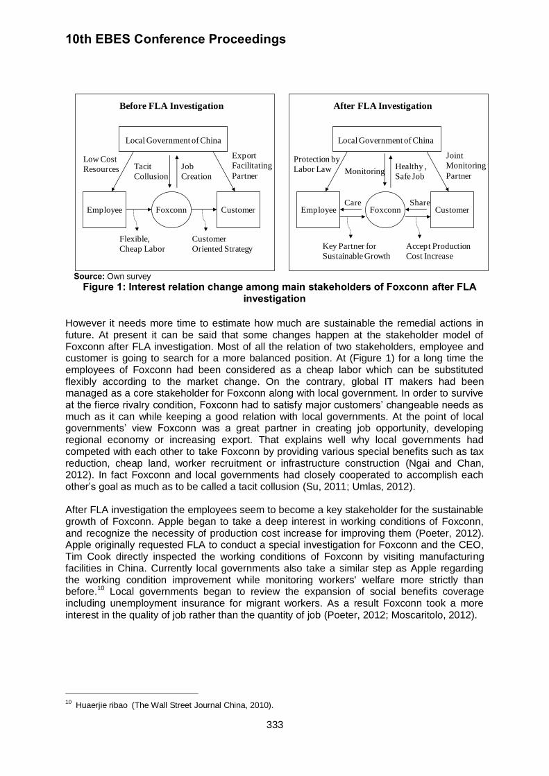
10th EBES Conference Proceedings
333
Before FLA Investigation
Local Government of China
FoxconnEmployee Customer
Flexible,
Cheap Labor
Customer
Oriented Strategy
Low Cost
Resources
Export
Facilitating
PartnerJob
Creation
Tacit
Collusion
After FLA Investigation
Local Government of China
FoxconnEmployee Customer
Key Partner for
Sustainable Growth
Accept Production
Cost Increase
Protection by
Labor Law
Joint
Monitoring
PartnerHealthy ,
Safe Job Monitoring
Care Share
Source: Own survey
Figure 1: Interest relation change among main stakeholders of Foxconn after FLA investigation
However it needs more time to estimate how much are sustainable the remedial actions in future. At present it can be said that some changes happen at the stakeholder model of Foxconn after FLA investigation. Most of all the relation of two stakeholders, employee and customer is going to search for a more balanced position. At (Figure 1) for a long time the employees of Foxconn had been considered as a cheap labor which can be substituted flexibly according to the market change. On the contrary, global IT makers had been managed as a core stakeholder for Foxconn along with local government. In order to survive at the fierce rivalry condition, Foxconn had to satisfy major customers’ changeable needs as much as it can while keeping a good relation with local governments. At the point of local governments’ view Foxconn was a great partner in creating job opportunity, developing regional economy or increasing export. That explains well why local governments had competed with each other to take Foxconn by providing various special benefits such as tax reduction, cheap land, worker recruitment or infrastructure construction (Ngai and Chan, 2012). In fact Foxconn and local governments had closely cooperated to accomplish each other’s goal as much as to be called a tacit collusion (Su, 2011; Umlas, 2012). After FLA investigation the employees seem to become a key stakeholder for the sustainable growth of Foxconn. Apple began to take a deep interest in working conditions of Foxconn, and recognize the necessity of production cost increase for improving them (Poeter, 2012). Apple originally requested FLA to conduct a special investigation for Foxconn and the CEO, Tim Cook directly inspected the working conditions of Foxconn by visiting manufacturing facilities in China. Currently local governments also take a similar step as Apple regarding the working condition improvement while monitoring workers' welfare more strictly than before.10 Local governments began to review the expansion of social benefits coverage including unemployment insurance for migrant workers. As a result Foxconn took a more interest in the quality of job rather than the quantity of job (Poeter, 2012; Moscaritolo, 2012).
10
Huaerjie ribao (The Wall Street Journal China, 2010).
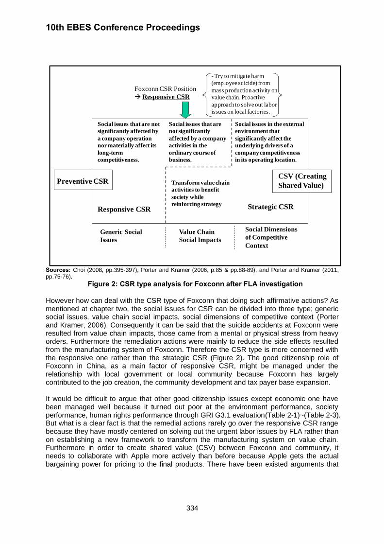
10th EBES Conference Proceedings
334
Generic Social
Issues
Value Chain
Social Impacts
Social Dimensions
of Competitive
Context
Preventive CSRCSV (Creating
Shared Value)
Responsive CSR Strategic CSR
Social issues that are not
significantly affected by
a company operation
nor materially affect its
long-term
competitiveness.
Social issues that are
not significantly
affected by a company
activities in the
ordinary course of
business.
Social issues in the external
environment that
significantly affect the
underlying drivers of a
company competitiveness
in its operating location.
Transform value chain
activities to benefit
society while
reinforcing strategy
Foxconn CSR Position
Responsive CSR
- Try to mitigate harm
(employee suicide) from
mass production activity on
value chain. Proactive
approach to solve out labor
issues on local factories.
Sources: Choi (2008, pp.395-397), Porter and Kramer (2006, p.85 & pp.88-89), and Porter and Kramer (2011, pp.75-76).
Figure 2: CSR type analysis for Foxconn after FLA investigation
However how can deal with the CSR type of Foxconn that doing such affirmative actions? As mentioned at chapter two, the social issues for CSR can be divided into three type; generic social issues, value chain social impacts, social dimensions of competitive context (Porter and Kramer, 2006). Consequently it can be said that the suicide accidents at Foxconn were resulted from value chain impacts, those came from a mental or physical stress from heavy orders. Furthermore the remediation actions were mainly to reduce the side effects resulted from the manufacturing system of Foxconn. Therefore the CSR type is more concerned with the responsive one rather than the strategic CSR (Figure 2). The good citizenship role of Foxconn in China, as a main factor of responsive CSR, might be managed under the relationship with local government or local community because Foxconn has largely contributed to the job creation, the community development and tax payer base expansion. It would be difficult to argue that other good citizenship issues except economic one have been managed well because it turned out poor at the environment performance, society performance, human rights performance through GRI G3.1 evaluation(Table 2-1)~(Table 2-3). But what is a clear fact is that the remedial actions rarely go over the responsive CSR range because they have mostly centered on solving out the urgent labor issues by FLA rather than on establishing a new framework to transform the manufacturing system on value chain. Furthermore in order to create shared value (CSV) between Foxconn and community, it needs to collaborate with Apple more actively than before because Apple gets the actual bargaining power for pricing to the final products. There have been existed arguments that
10th EBES Conference Proceedings
335
Apple has to take more responsibility to access labor issue, and engage in more deeply for creating share value between business and community in China.11 5. CONCLUSION The biggest electrical manufacturing service provider in global electronic industry, Foxconn faces a turnover period after employee suicide accidents. The change goes toward the recovery of employees’ interest. At the introduction part three questions were suggested, and each corresponding answer can be summarized as below. Firstly there had been a clear recognition gap between Foxconn and third-party evaluators at least before late 2011, and this study reviewed it through GRI G3.1 indicator and FLA investigation report. According to the GRI G3.1 indicator analysis, Foxconn CSER report covered all of the articles in profile disclosures part but just covered 44% among total 84 articles in performance indicators part. Therefore it can be said that Foxconn CSER report does not exactly reflect a real condition but only presents what Foxconn wants to show. In addition according to FLA investigation report, most employees of Foxconn had done overtime works during the peak season without adequate rest or proper compensation. Student intern system was also unfavorable for their working conditions because legal status of interns was not employee nor student. Further the immobility of social benefit system under household registration institution restricted the unemployment insurance coverage for migrant workers. On the contrary, the dormitory labor system of Foxconn was very useful to control workers’ lives not only at workplace but also at private living space. Through the dormitory labor system Foxconn was able to make a just-in-time, speedy & flexible manufacturing business. But it was difficult for local employees to share their opinions or hardships with other roommates under the system. Such a less interaction among workers resulted in the disinterest for labor union. Secondly after FLA investigation Foxconn has successfully completed remedial tasks as of June 2012. Foxconn intends to make the interest relation of two stakeholders, employee and customer move a more balanced position. Recently such remedial actions can be considered as a restoration process for employees’ benefit that had been infringed by other two stakeholders, customer and local governments. Chinese local governments have also taken a similar step as global IT firms to tackle the working condition issues while monitoring them more strictly than before. Thirdly the CSR type of Foxconn can be considered as the responsive CSR even though remedial actions have been successfully taken. The suicide accidents resulted from mental or physical stress by the tough manufacturing system, and most of remedial actions were targeted for mitigating the negative effects of it. Finally the implication of this study would be summarized as below three points. Above all it needs to reconsider the real value of local labor in China because it is not cheap labor nor freely substitutable resource any more. The reconsideration is required not only for high skilled engineers but also for repetitive assemblers at production line. So it needs a turnover of existing management behavior with pursuing a cost leadership through the labor cost reduction in China. Now Chinese local workers, especially young workers under 25 years old sincerely hope to be recognized as a unique personal prior to be just a cheap labor. It is time for global firms should manage them as one of critical business partners. This is the second implication. Recently most global companies much more emphasize each employee’s
11
Despite remedial actions made by Foxconn and Apple to improve working conditions, some labor groups remain unconvinced that Apple should take much more responsibility. Students & Scholars Against Corporate Misbehavior (SACOM) has criticized FLA report for supposedly omitting details for harsh management practices, work stress, and student intern abuse (Poeter, 2012; Umlas, 2012).
10th EBES Conference Proceedings
336
voluntary participation, taking initiative or entrepreneurship to maximize the organizational creativeness or the operational efficiency. Chinese local workers might not be an exception to such a global trend. The third implication is that the institutional factor is still very important in doing a business in China. Foxconn could accomplish a rapid growth in China through a close partnership with local governments. Regardless of ethic management issues, Foxconn has understood very well Chinese unique institutional factors like student intern system or household registration system, and it used such factors effectively in creating the competitive advantage. Among six stakeholders, local government is more concerned with institutional factor than any others, therefore it needs to take an in-depth consideration for the dynamic nature of it as Foxconn has done in China.
REFERENCES Chan, D., 2011. Activist perspective: The social cost hidden in the Apple product. Journal of Workplace Rights, 15(3-4), pp.363-365. Choi, B.H., 2008. A study on the type and impact of Corporate Social Responsibility(CSR) in China: Focusing on the CSR Activities for Toyota, Volkswagen, GM. The journal of Chinese Studies, 45(September), pp.387-422.
Choi, B.H. and We, O.G., 2008. A study on the corporate Social Responsibility(CSR) reinforcement in China: Focusing on Chinese automobile industry. International Area Review, 11(2) (November), pp.33-54. Deffree, S., 2011. Foxconn explosion ignites conversation on corporate responsibility. EDN. Comment(June 23), p.8.
Diyi caijing ribao (FT Chinese Daily), 2010. Workers unveil the inside story of sweatshop
issue for Foxconn, the continuous 12 hours’ standing at machine (in Chinese). Fair Labor Association, 2012a. Independent investigation of Apple supplier, Foxconn Report, (March), pp.1-13, Available at: <http://www.fairlabor.org/sites/default/files/documents/reports/foxconn_investigation_report.pdf> [Accessed 17 September 2012]. Fair Labor Association, 2012b. Foxconn verification status report, (August), pp.1-3, Available at: <http://www.fairlabor.org/sites/default/files/documents/reports/foxconn_verification_report_final.pdf> [Accessed 7 October 2012]. Global Reporting Initiative, 2011. Sustainability reporting guidelines; Version 3.1, (March), pp.1-49, Available at: <https://www.globalreporting.org/resourcelibrary/G3.1-Guidelines-Incl-Technical-Protocol.pdf> [Accessed 12 October 2012]. Foxconn Technology Group, 2012. Foxconn 2011 CSER annual report, (June), pp.1-51. Foxconn Technology Group, 2011. Foxconn 2010 CSER annual report, (September), pp.1-79.
10th EBES Conference Proceedings
337
Guo, L., Hsu, S.H., Holton, A., and Jeong, S.H., 2012. A case study of the Foxconn suicides: An international perspective to framing the sweatshop issue. International Communication Gazette, 74(5), pp.484-503.
Ha, H.J., 2011. Major contents for revision of GRI G3.1 guideline. Sustainability Issue Papers,
122 (May 11), pp.1-11. Hermanson, J., 2011. Activist perspective: Engaged sociology and labor's struggles. Journal of Workplace Rights, 15(3-4), pp.421-423.
Huaerjie ribao (The Wall Street Journal China), 2010. Suicide accident of Foxconn causes Chinese government to take a deep interest (September 20) (in Chinese). Jang, S.W., 2012. A hidden giant of IT industry, Hon Hai. SERI Management Note, 150(May 18), pp.1-10. Jang, S.K. and Seok, S.H., 2007. The evolution and new integral approach on CSR.Gyungyong Sahak, 22(3), pp.261-284. Jeong, W.Y., 2006. Corporate social responsibility, For whom and what to do? Gyungyonggea, 336(December), pp.40-41. Kam, D.S., 2010. Review for change stream of manufacturing model through Apple and Hon Hai. LG Business Insight, (May 5), pp.2-15. Kaku, R., 1997. The Path of Kyosei. Harvard Business Review, (July-August), pp.55-63.
Kim, H.R., Kim, N.M., Yoo, K.H., and Lee, M.K., 2005. Developing a scale for evaluating corporate social responsibility. Marketing Research, 20(2), pp.67-87.
Kwak, K.H., 2006. Corporate Social Responsibility(CSR) and capital market. Commercial Law Studies, 25(3), pp.113-163.
Martin, R., 2002. The virtue matrix: Calculating the return on corporate responsibility. Harvard Business Review, (March), pp.69-75. Martin, R., 2010. The age of customer capitalism. Harvard Business Review, (January-
February), pp.58-65. Moscaritolo, A., 2012. Foxconn settles wage dispute with workers in China. PC Magazine,
(January), p.1. Nanfang ribao (NF Daily), 2010. Monthly minimum wage for 80% of general workers in
Foxconn will get to two thousand RMB (October 18) (in Chinese). Ngai, P. and Chan, J., 2012. Global capital, the state, and Chinese workers: The Foxconn Experience. Modern China, 38(4), pp.383-410.
Poeter, D., 2012. Foxconn, Apple to Share Chinese factory improvement costs. PC Magazine, (May), p.1.

10th EBES Conference Proceedings
338
Porter, M.E. and Kramer, M.R., 2002. The competitive advantage of corporate philanthropy. Harvard Business Review, (December), pp.57-68.
Porter, M.E. and Kramer, M.R., 2006. Strategy & society: The link between competitive advantage and corporate social responsibility. Harvard Business Review, (December),
pp.78-92. Porter, M.E. and Kramer, M.R., 2011. Creating share value: How to reinvent capitalism & unleash a wave of innovation and growth. Harvard Business Review, (January-February),
pp.62-77. Rulliat, A., 2010. The wave of suicides among Foxconn workers and the vacuity of Chinese Trade Unionism. China Perspectives, 3(November), pp.135-137.
Smith, R., 2011. Productive factory towns. Research∙Technology Management, (March-April),
pp.55-56. Su, Y.H., 2011. Student workers in the Foxconn Empire: The commodification of education and labor in China. Journal of Workplace Rights, 15(3-4), pp.341-362.
Umlas, E., 2012. How Apple, Foxconn, and others can address labor abuses in overseas factories. Christian Science Monitor, (April 9), pp.1-3.
10th EBES Conference Proceedings 23 - 25 May, 2013. NIPPON HOTEL, ISTANBUL, TURKEY ISBN: 978-605-64002-1-6. WEBSITE: www.ebesweb.org
339
MOBBING IN ORGANIZATIONS
NEVRA SANIYE GUL Institute of Social Sciences
Istanbul Commerce University Turkey
A. TUGBA KARABULUT Faculty of Commercial Sciences Istanbul Commerce University
Turkey [email protected]
Abstract: This paper aimed to define characteristics, factors, directions of mobbing through
literature review. Furthermore, mobbing laws of Turkey and selected EU countries were presented. Human factor started to be meaningful with Behavioral Approach in management. Hawthorne Studies highlighted the conclusion that human relations and social needs of workers were crucial aspects of management. Human is the most important factor which increases productivity. Thus, motivation and all other efforts are needed to use this factor efficiently. Herzberg’s studies and McGregor’s Theory Y improved the understanding related to motivation. Leymann who is a professor and practising psychologist identified mobbing as one of the issue which effects the human factor in management. Effective management of mobbing can significantly reduce its impacts. It can be possible if the organizations’ employees and employers are aware about its characteristics, identify its impacts and develeop management system to prevent its reasons. Although significant studies has been conducted in the field of mobbing, most of the models discuss its limited aspects. This paper is expected to increase awareness about mobbing and lead researchers to develeop a management system to prevent its reasons. Keywords: Mobbing, Management Theories, Mobbing Laws
1.INTRODUCTION Understanding human is a substantial issue which has been discussed by management, economics, psychology, history, anthropology and sociology. Personality of people affect their behaviors and relations in the work place. Employees can be victims, perpetrators or observers interms of mobbing. Behavioral Approach started to analyze human factor in management by considering employees as individuals, assets and resources to be improved and worked with. Employees were considered like machines in Classical Approach. Hawthorne studies highlighted the conclusion in Behavioral Approach by explaining that human relations and social needs of employees were important aspects of management (Wren, 2005). External and internal forces can energize, direct and sustain behavior of employees by increasing their motivation to increase productivity. Although, characteristics of individual and job are important forces for motivation, psychology of an employee is the most important factor indirectly related with the social environment of the work (Hitt et al. 2009).
Although personality is affected by both heredity and environment, personality disorders are learning disorders. Some of these disorders cause personality to have unrealistic perception

10th EBES Conference Proceedings
340
of “ rights” and “responsibilities. Thus, people who have personality disorders can expect their needs and preferences need to be satisfied before others’. These people are insensitive to rights and previleges of others. They’ll be bossy, dominating, threatening and even violent if they feel that their rights are threatened. They can whine, complain, feel angry and resented when they do not get what they want (Capozzoli and McVey, 1996, p.37). When
employees develop relations with other employees at work; ambitions, conflicts, arguments, negotiations, violence, and expectations are unavoidable. Mobbing which is one of the most important problem in the work environment occurs due to an event through any hierarchical level and continue systematically. It may end with physical and psychological damages on the employee. It may cause unemployment of this person in the rest of his/her life. According to EU27 Countries report, 43% of mobbing claims were identified as bullying whereas 54% of them were identified as verbal abuse (Eurofound, 2012).
2.THE DEFINITION OF MOBBING Researchers who studied in the fields of management and organizational psychology found out an issue which cause low performance, absentism, lay off, early retirement. It is related with work problems. “Mobbing” was translated from Latin word “mobile vulgus” which means undetermined crowd, violent group. It means to crowd around, jostle or annoy from this point of view (Halsey, 1988, p.652). Leymann is the first researcher who identified “mobbing” as “ganging up on someone” or psychic terror. His definition is as follows: “It occurs as schisms, where the victim is subjected to a systematic stigmatizing through, interalia, injustices (encroachment of a person’s rights), which after a few years can mean that the person in question is unable to find employment in his/her specific trade. Those responsible for this tragedic destiny can either be workmates or management” (Leymann, 1990, p.119). The definition is based on two terms; Schism which is sect or group formed by a division (Halsey, 1988, p.890), stigmatizing which is to mark or token of shame (Halsey, 1988, p.980). Mobbing occurs in the group of people who think they are selective and ready to obey the mobber’s thoughts while he/she is attacking to the marked person who is different from the group. Bullying, stalking, psycho-terror at workplace, emotional abuse, work or employee abuse, victimization, intimidation, verbal abuse, and psycho-violence are words which are used for mobbing in the literature (Ozkul and Carikci, 2010, p.1).
Operational definition of mobbing is as follows; “physical terror or mobbing in working life means hostile and unethical communication which is directed in a systematic way by one or a number of persons mainly toward one individual” (Leymann, 1990, p.120). Sytematic,
frequent, repetitive attacks cause considerable and unavoidable physic, psychosomatic and social misery. 3. THE LITERATURE REVIEW Mobbing was used for the first time in an observation of Lorenz to define the attack of a group of small animals to frighten a bigger animal.in 1960s. Leymann is a pioneer professor and practising psychologist who used mobbing for the work place in 1984. Bullying is used in 1983 in Norway to define acts of students in the school which cause suicide of three teenagers (Tetik, 2010, p.81-82).

10th EBES Conference Proceedings
341
Einarsen defined bullying as a widespread phenomenon in many countries. He added that “3%-4% of employees were exposed to bullying in Scandinavia” (Matthiesen and Einarsen,
2007, p.735). On the other hand, 5% of employees declared that they were mobbed at their workplace in Spain. Carnero et al. (2010) found out that some personal characteristics, job characteristics and
working conditions were significant to explain the probability of being a mobbing victim. They added that differences in these variables depend on the victim's gender. On the other hand, Leymann developed LIPT questionnaire (Leymann Inventory of Psychological Terror) which includes 45 activities of mobbing. LIPT questionnaire is based on five categories to identify the existency of mobbing (Carnero et al. 2010, pp.3777-3786): (A) Activities on possibilities of the mobbed person or mobbing victim to communicate adequately: It questions the communication channels of the victim. E.g.: If he/she is silenced or continously interrupted, suffers from verbal attacks at work life or in personal life, verbal or written threats etc. (B) Activities on possibilities of the victim to maintain his/her personal reputation: It is the isolation against the victim such as physical presence of the victim is denied. (C) Activities on possibilities of the victim to maintain his/her personal reputation: Attacks on the reputation of the victim as gossips or sayings about his/her mental health. Stigmatizing is the main issue of this category. Nationality, religion, and sex discrimination are questioned as well. (D) Activities on the occupational situation of the victim: It questions if victim is deprived from any activity; given meaningless, or difficult work assignments which are far above his/her capacity. (E) Activities on the physical health of the victim: It questions the physical condition of the situation as if there is an attack physically on the victim by giving dangerous work assignment, threats or sexual attacks. Two critical events are mostly discussed in mobbing researches; conflict and violence. Conflict is an emotional struggle of opposing impulses or desires within and struggle between two forces (Halsey, 1988,p. 211). The real reason why mobbing occurs at workplaces is unknown however, in some cases, the victim is apparent when one party to the conflict gains upper hand (Leymann, 1990, p.121). Violence is a great physical force to harm, instance of violent or injurious treatment (Halsey, 1988,p. 1113). Lewis explained terms of nuisance, conflict, hostility and violence as follows (Lewis, 2004, p.46); “Nuisance behavior may be annoying and offensive to others but does not have any direct malicious intent to a specific individual or group. Examples might be offensive gestures, swearing, off-color jokes and graffitti….Conflict refers to the normal disagreements that take place in all interpersonal relationships...Hostility refers to acts that are nonphysical but are directed at an individual or group with the intent of inflicting some type of emotional harm. Examples of this are harassment, discrimination, stalking, verbal threats, comments, acts of intimidation, etc. The defining characteristics is that there is no bodily contact or destruction of property. However, violence involves the display of physical force against a person or property with the intention to do personal injury or destruction to property.”
4.THE STRUCTURE, FACTOR, TYPES AND DIRECTIONS OF MOBBING According to Leymann (1990), there are four critical incident phases for mobbing; Phase 1 - The Original Critical Incident. It is the shortest phase which ends with the stigmatizing actions on the focused victim. The observation is the conflict.

10th EBES Conference Proceedings
342
Phase 2 - Mobbing and Stigmatizing: Manipulation is the characteristic to get at a person or punish him/her. The manipulation is based on reputation of the victim, communication toward the victim, isolation, humiliating work tasks, violence and threats of violence. Phase 3 - Personnel Administration: Management takes over the prejudices of the victim’s workmates. Management assumes that the cause of the problem lies in the deviant personality of the victim and prefers to get involve the situation and get rid of the victim. Phase 4 - Expulsion: Victim is expelled from working life. He/she faces with further stigmatizing as long-term sick leave, no work provided, relocation to degarding work tasks and psychiatric treatment. Mobbing is considered as strategic mobbing when the mobber is the manager or the boss and his/her actions are due to cost-benefit considerations. It is considered as horizontal mobbing when the perpetrator/s is/are colleague/s and his/her/their actions are due to social reasons. Although, the management doesn’t represent the harasser, there is a high risk that it supports the perpetrator or ignores the violence, thus it leades to a double victimisation of the mobbed (Ferrari, 2004). Three types of mobbing are considered depending on the link between victims and aggressors: horizontal, up-down and down–up mobbing. Up-down mobbing occurs when a superior harasses one of his subordinates. Down-up mobbing occurs when a subordinate or group of subordinates harass his/her/their superior. Horizontal mobbing occurs among co-workers at the same hierarchical level (Carnero et al. 2010,
p.3786). On the other hand, horizontally-by mobbing occurs when employees are against a colleague, the victim is against the employer, employer is against the perpetrators, and victim is against the perpetrators (Ramage, 1996). Factors which cause mobbing at the work place are as follows; inequality, undefined authority and rules that may prevent attacks of mobber. Individual factors which can apply to both the perpetrator and to the victim such as socio-demographic variables, personality characteristics, traits, behaviours, and characteristics of the individual’s affiliation with their workplace. Situational factors such as working in jobs with an unequal sex ratio, differences in power which have formal or informal nature, job insecurity, change of supervisor, working in businesses with a high customer service which may cause mobbing by clients. Organizational factors such as leadership and management, organizational change, culture and climate, job complexity and control, stressful work environments, conflict and ambiguity of work roles. Societal factors: Violent crime in society, economic and social changes, immigration and informal economic sector (Ferrari, 2004).
5. LAWS AGAINST MOBBING EU The advantages of the existence of regulation and legislation are as follows: (1) the problems of violence and harassment at work become more visible; (2) the awareness and recognition of the problems increase; (3) discussion in an organisation is encouraged and increased. Workers’ security feeling is increased. Laws are forces which oblige organisations take actions to prevent and handle the violence problems (European Agency for Safety and Health at Work, 2009) Code of Obligations (6098)1 regulates employers' liability regarding mobbing under Article 417 which imposes duties on employers to protect their employees from mobbing. An employer is responsible for keeping order in the workplace in accordance with the principles
1 http://www.resmigazete.gov.tr/eskiler/2011/02/20110204-1.htm (In Turkish).
10th EBES Conference Proceedings
343
of honesty; protecting and respecting the personality of the employee; taking measures to guarantee that employees do not encounter sexual or emotional abuse and protecting those who have encountered such abuse from further suffering (Yuksel and Akyurek, 2012).
There are laws in several EU countries related to mobbing. Some of them are as follows: The Labor Code in France states that “no employee must be subjected to repeat deeds of moral harassment aimed at or leading to a deterioration of working conditions likely to detract from the rights of employees and their dignity, to undermine their physical or mental health or to compromise their professional future” (Article 1152-1, Article 1152-4, 1.5.2008). According to Section 27-Threat of Violence in Finland “The work and work conditions in jobs entailing an evident threat of violence shall be so arranged that the threat of violence and incidents of violence are prevented as far as possible. Accordingly, appropriate safety arrangements and equipment needed for preventing or restricting violence and an opportunity to summon helps shall be provided at the workplace”. On the other hand, The Working Environment Act, Section 4-3 in Norway states that “Employees shall not be subjected to harassment or other improper conduct”. The Belgian Law of Well-being (2007) indicates ‘moral harassment’. Its definition is framed in a broader definition of psychological aspects. It mentions the duration and the multiplicity of abusive conduct. The employer has to deal with third-party violence and organise psychological support. If in-company procedure fails, external procedures exist to settle the issue. Section 3 AGG in Germany explains that “harassment shall be deemed to be discrimination when unwanted conduct, in connection with any of the grounds referred to under Section 1, takes place with the purpose or effect of violating the dignity of the person concerned and of creating an intimidating, hostile, degrading, humiliating or offensive environment. Mobbing is addressed in the Polish Labour Code as ‘action or behaviour concerning an employee or directed against an employee which consists in a persistent and long-lasting harassment of or threats to the employee and which results in a reduced self-assessment of his or her professional abilities and which cause, or are aimed at, humiliating or ridiculing the employee, isolating or eliminating him or her from their group of co-workers’ (Division IV, Article 94, Section 2).(European Agency for Safety and Health at Work, 2009, 29-32). As it is observed, there are laws against mobbing in several EU countries. Situations involving a threat or act of violence are preceded by signs of trouble which can be on a system level such as grievances which indicate poor morale or labor-management conflict. An employee can complain for harassment or reported domestic abuse. If the company leadership responds to danger signals, it can handle them by discipline system, labor relations, security or occupational health systems. It has to take direct action when the crisis has blown up (Braverman, 1999, p.12-13).
Mobbing in the workplace has severe consequences on victims, witnesses, businesses and society. Stress, physical and mental illnesses, anxiety, lack of initiative and motivation, absenteeism which affect victims, their colleagues, families and friends. It has also a high economic impacts on the business and health sector. Mobbing causes organisational problems, premature retirement, sickness absence, replacement costs due to labour turnover, decreased performance/productivity, and loss of public reputation. The society will be affected by social and economic costs (Ferrari, 2004).
6. CONCLUSION Mobbing has harmful effects on employees, organizations and society. Individuals face psychological illnesses and organizations loose their key employees due to mobbing. If employees are not happy and satisfied about working conditions of the organization, they can talk about mobbing practices which they are exposed to destroy reputation of the
10th EBES Conference Proceedings
344
organization. Besides, employees may sue the organization which may cost more to the organization than trying to prevent mobbing. Observers will loose their trust to the organization. They will be worried about the possibility that they will be exposed to the same mobbing practices. The performance and efficiency of the organization will also be decreased. Conflicts among employees will be increased. There will be negative organizational climate, low confidence, decline in respect and creativity due to demoralization. Economic cost of the mobbing to the organization are caused by increase in absentism, loss of qualified employees, decrease in employee performance and work quality, compensation costs to the victim due to the cases, cost of sues, and early retirement payments. Turkey needs to develop and practice appropriate legislative framework to protect rights of employees, get rid of harmful effects of mobbing and facilitate peace in organizations.
REFERENCES Braverman, M., 1999. Preventing Workplace Violence. New Delhi: Sage Publications.
Capozzoli, T. and McVey, S., 1996. Managing Violence in the Workplace. Florida: St.Lucie Press. Carnero, M.A., Martinez, B., and Sanchez-Mangas, R., 2010. Mobbing and Its Determinants: The Case of Spain. Applied Economics, 42(29), pp.3777-3787.
Eurofound, 2012. Fifth European Working Conditions Survey. Luxembourg: Publications Office of the European Union. European Agency for Safety and Health at Work, 2009. European Risk Observatory Report, Workplace Violence and Harassment: a European Picture. [online] Available at: <https://osha.europa.eu/en/publications/reports/violence-harassment-TERO09010ENC> [Accessed 3 March 2013]. Ferrari, E., 2004. Raising Awareness on Mobbing: An EU Perspective. European
Commision, DAPHNE Programme: Preventive Measures to Fight Violence Against Children, Young People and Woman. Halsey, W., 1988. Macmillan Contemporary Dictionary. New York: ABC.
Hitt, M.A., Black, J.S., and Porter L.W., 2009. Management. New Jersey: Pearson International Edition. Lewis, G., 2004. Violence at Work: Causes and Protection. In: J. Thomas and M. Hersen, eds. Psychopathology in the Workplace: Recognition and Adaptation. New York: Brunner-
Routledge, pp.313-328. Leymann, H., 1990. Mobbing and Psychological Terror at Workplaces. Violence and Victims, 5(2), pp.119-126 Matthiesen, S.B. and Einarsen, S., 2007. Perpetrators and Targets of Bullying at Work: Role Stress and Individual Differences. Violence and Victims, 22(6), pp.735-753.

10th EBES Conference Proceedings
345
Ozkul, B. and Carikci, I.H., 2010. Mobbing ve Turk Hukuku Acısından Degerlendirilmesi [Mobbing and Its Evaluation in temrs of Turkish Law]. Suleyman Demirel Universitesi İ.İ.B.F. Dergisi, 15(1), pp.481-499.
Ramage, R., 1996. Mobbing in the Workplace. New Law Journal. 146, 1538(1532). [online]
Available at: <http://www.law-office.demon.co.uk/art%20mobbing-1.htm> [Accessed 3 March 2013]. Tetik, S., 2010. Mobbing Kavramı: Birey ve Orgutler Acısından Onemi [Mobbing Concept and Its Importance in Terms of İndividuals and Organizations]. KMU Sosyal ve Ekonomik Arastırmalar Dergisi, 12(18), pp.81-89 Yuksel, M.O. and Akyurek, K.C., 2012. ‘Mobbing' Under Turkish Law: Remedies and Precautions. [online Available at: <http://www.internationallawoffice.com/newsletters/detail.aspx?g=0f945a73-c0be-4de6-8418-49ee0f6e2732&redir=1> [Accessed 3 March 2013]. Wren, D.A., 2005. The History of Management Thought. New Jersey: Wiley.
10th EBES Conference Proceedings 23 - 25 May, 2013. NIPPON HOTEL, ISTANBUL, TURKEY ISBN: 978-605-64002-1-6. WEBSITE: www.ebesweb.org
346
SYSTEM MODELING OF REGIONAL ECONOMIC PROCESSES DYNAMIC ON THE BASE OF THE
INFORMATION MODELLING TECHNOLOGY
ALEXANDRE BOULYTCHEV Laboratory of Information modeling
Institute for Systems Analysis of Russian Academy of Sciences Russia
VLADIMIR BRITKOV Laboratory of Information modeling
Institute for Systems Analysis of Russian Academy of Sciences Russia
Abstract: In the article from the global modeling positions of the regional dynamic (Britkov
and Gelovani, 2003) – the developed countries of North America (USA, Canada), Western and Eastern Europe (Great Britain, Germany, France, etc.), carried out at Institute Of Systems Analysis, is considered the process of the institutional structures formation, their correlation and relationship with macroeconomic indicators dynamics scenarios. Macroeconomic indicators are considered as the indicators reflecting an economy and welfare development level of the countries. Keywords: Information Modeling, Data Mining, Bayesian Methods 1. INTRODUCTION Modelling of dynamics of economic systems in the conditions of global integration of financial, production and information resources becomes actual in connection with complication of structure and functions of communications between economic systems and their components. In the majority of tasks development of methods which define the hidden factors influencing dynamics of processes and in particular change of influence of various factors on process as a whole is necessary for formalization of the difficult systems dynamics scenarios. Thus, the actual task consists in creation of scenarios of dynamics of difficult economic systems and formalization of processes. System approach, methods of the intellectual analysis of data, technologies of parallel calculations (Emelyanov et al. 2005) and use of information resources from the global computer environment is applied to the solution of an objective. We considered Data mining information technology of intellectual data analysis and formalization of new knowledge. As it is shown in work the approach, includes methods of application of the operator equations, Bayesian estimation and classification, the composite (aggregated) models for forecasting. New knowledge and the opened regularities received by means of expansion of a set of methods of the analysis of data are necessary for search and formalization of system regularities in difficult systems (Britkov and Boulytchev, 2010).
In work the technology of global modelling (Britkov and Gelovani, 2003) of economic
processes are developed. As the basic the technology of system-integral modelling is used.
10th EBES Conference Proceedings
347
For identification of parameters of models with an assessment of their aposteriorny distributions multidimensional Bayesian qualifiers are used. 2. PROBLEM DEFINITION The present stage of development of information technologies offers users large volume of information resources for the analysis and a set of the formalized models of management of difficult systems. In certain cases for adoption of the correct decisions it is necessary to investigate a large number of models to define the most probable scenario of changes of system (Britkov et al. 2011). At implementation of the project the theoretical reserve in the
form of formalization of the principles of creation of scenario information models of dynamics of difficult systems is created:
1) it is postulated existence of integrated parameters of systems (reflecting dynamics of a condition) in the form of implicitly set function on multidimensional space of characteristics of the generalized structure of system (a subsystem, their function, communication in system and with environment) and possessing property of preservation of quasiconstant values is postulated at preservation of conditions of system (when the generalized structure of system don't undergo considerable changes for a certain period). Integrated parameter is empirically on the basis of aprioristic assumptions and the numerical analysis of data. It follows from this that integrated parameters accept discrete values – a time interval of change of values much less interval of preservation of values;
2) aprioristic identification of integrated parameters for creation of information models. Integrated parameter often is the target variable for which the task of creation of the scenario forecast is set. For example, an inclination in the logarithmic scale of a trend of gross domestic product (gross domestic product) concerning a timeline for the various temporary periods, the cycle gross domestic product period concerning a trend, the same characteristics for gross domestic product per capita, population, a salary, limit productivity, etc.;
3) the analysis, classification and creation of ontology of existing models of information modeling. One of traditional approaches in information modeling consists in creation of a class of well-founded (adequate) system and integrated models which belong to the ordinary differential equations of the first order where it is used the integrated aggregated macroeconomic parameters (Boulytchev and Britkov, 2011) identified at
the previous stage: ' ( , , , )x f x p , where: x - vector of integral macroeconomic
indexes of system, - vector of controlling parameters, p - vector of model
parameters, - vector of accidental stochastic influences. Creation and verification
of models happen on the basis of integrable economic data from the global information environment (Emelyanov et al. 2005) (data from several official sources
are used: services of statistics of the countries, data of independent rating agencies, data of World Bank);
4) determination of an explicit type of the functional dependences between variables and their derivatives and the subsequent incorrect identification of parameters of models on different time slots is difficult as system generalized structure often it is unknown. For overcoming of the specified difficulties as basic models for scenario prediction of integral indexes the developed compositions of multivariate Bayesian well-grounded stochastic models with an assessment of posterior probabilities and different classes of decisive rules (averaging, bootstrap, selection of models, etc.)
are used. Let ( , )p y - a joint density function of distribution of probabilities for a
vector of accidental observations y and a vector of parameters . Model
10th EBES Conference Proceedings
348
coefficients, mathematical expectations or dispersions, etc. can be components of . Then ( | ) ~ ( | ) ( )p y p y p .
This is a posteriori Function of a vector of parameters on condition of the given selective information — prior Credibility Function for a vector of parameters. - Credibility Function. The assessment of expected Credibility Function for statuses of objects of system which weren't watched yet in the assumption that generates the same process and the parameters
characterizing process the same that in original process looks like: ( | )p y — posteriori
Credibility Function of a vector of parameters on condition of the given selective information
y , ( )p — prior Credibility Function for a vector of parameters . ( | )p y (function ) -
credibility function. The assessment of expected Credibility Function for statuses of objects of
system which weren't watched yet in the assumption, that y generates the same process
and the parameters characterizing process the same that in original process, then we have:
( , | ) ( | , ) ( | )p y y p y y p y , (1)
( | ) ( , | ) ( | , ) ( | )R R
p y y p y y d p y y p y d
, (2)
( | ) ( | )R
P y R y p y y dy (3)
At the following stage as a result of integration of information and analytical resources stochastic predictive models of dynamics of the difficult systems, intended for operation with the distributed information and analytical resources are constructed. Simulation of global processes of dynamics of structures of economic systems over the countries and regions is made: Russia, CIS countries, country of Eastern Europe and Western Europe (Great Britain, Germany, France, etc.) countries of North and South America (separately USA, Canada), countries of South East Asia (separately Japan). Factors of dynamics of economic production and scenarios of economic development of Russia for 2012-2025 are specified. Project deliverables can be used in case of creation of computer support systems of decisions in modules of predictive simulation and optimization. The developed methods allow to carry out adjustment of dynamics of difficult systems and processes proceeding in them, in particular, use of results for scenario prediction of emergency situations for the territories of Russia is planned. As target variables for which there is a creation of scenarios, the aggregated macroeconomic indexes are used. Software modules of data analysis are constructed on the basis of technology of system simulation which implies creation and subsequent associations in classes of well-grounded stochastic models. Integral macroeconomic indexes are understood as indexes of a status of system which accept the discrete values (for example, an inclination in the logarithmic scale of a trend of gross domestic product concerning a time line for the different temporal periods, etc.). Creation of dependences and verification of global models happen on the basis of economic data from the global information environment (data from several official sources are used: services of statistics of the countries, data of independent rating agencies, data of World Bank). Correction of the data by the selected basis year is carried out. Classical approach in the analysis of initially heterogeneous data (different economic indexes) implies procedure of formalization of prior assumptions of that, dependences between what indexes will be analyzed with the subsequent creation and check of
10th EBES Conference Proceedings
349
hypotheses of nature of these dependences. In approach offered in operation creation of compositions of hypotheses of a choice of macroeconomic indexes is made for simulation and creation of system and integral models. The creation purpose - calculation of probably bigger range of dependences between indexes, testing and a choice of hypotheses (about optimum by criterion of competence of closeness of values of integral indexes to the actual indexes taking into account a type of distributions). Simulation of global processes is made separately over the countries: Russia, CIS countries, country of Eastern Europe and Western Europe, country of North and South America (separately USA), countries of South East Asia (separately Japan). The purpose of operation is determination of strategy of increase of efficiency of functioning of difficult modern economic systems. Besides in the conditions of uncertainty - scenario prediction of dynamics of trends of integral indexes of economic macrosystems on the basis of global simulation of dynamics of group of regions – the developed countries of North America (the USA, Canada), Western and Eastern Europe (Great Britain, Germany, France, etc.). The purpose of operation defined tasks:
1) the analysis of historical economic data from different time slots and creation of scenarios (look rules "if"), the known formalized economic laws adding ontology;
2) the analysis of causes and effect relationships between integral macroeconomic indexes;
3) the analysis of causes and effect relationships between the institutional and structural device of economy and scenarios of dynamics of macroeconomic indexes.
Subject is the analysis of the reasons of a discrepancy of rates of economic growth between the designated groups of the countries. For increase of efficiency of computation use of the concept of distributed computing environments which allows to apply mathematical models and computing methods to multisequencing of computation is offered. This concept sets the purpose to provide separated access to the various distributed computing resources and to provide means of coordinate use of resource data for the solution of a wide range of application-oriented computing tasks. The analysis of opportunities of the IARnet tools shows efficiency of application of approach to integration of information and algorithmic resources in GRID – computation for applications in the field of economic simulation (Emelyanov et al. 2005). Use of the MathCloud project which represents the mathematical environment which integrates the dedicated components being in the Internet is perspective also. Components of the environment are services of the solution of mathematical tasks, client applications and system components which allow to increase efficiency of calculating processes significantly. As input data integral characteristics are considered: Gross domestic product (final product), gross domestic product per capita, population, a salary, limit productivity. Groups of the countries are selected: Western Europe and colonies, Japan, Latin America, Eastern Europe, Asia, Africa etc. Traditional approach for prediction of integral characteristics consists in creation of several models in the form of systems of ordinary differential equations (or in private derivatives), research of behavior of phase paths depending on parameters and boundary conditions. The task is set - to define a temporal point (or an interval) after which the discrepancy of dynamics of macroeconomic indexes at the different countries and the reason which caused this discrepancy began. One of methods which allows to solve successfully the designated problem, iterative Bayesian estimation and associations of hypotheses in composition models is. The method doesn't assume prior knowledge of a type of multivariate distribution of integral characteristics. In the course of iterative training the system accumulates knowledge and allows to find not characteristic for last deviation from a path (a trend and

10th EBES Conference Proceedings
350
cycles) developments. In the tasks connected with "the reverse probability", on the basis of the data containing in selection, it is necessary to find parameters of the accidental process which consequence are these data. In "direct" tasks parameters of accidental process are known, on the basis of it probable statements concerning the outcomes generated by process are made. In our case of the task of data analysis and statistical estimation treat tasks on "the reverse probability". It is supposed that data for the analysis have the continuous range. (1), (2) и (3) – Bayesian theorem.
( , ) ( | ) ( ) ( | ) ( )p y p y p p y p y (4)
)(
)()|()|(
yp
pypyp
, где dpypyp )()|()( (5)
)()|(~)|( pypyp (6)
If we have data, for example, it can be gross domestic product, then ( | ) ( | ) ( )p y p y p
in accordance with (6). If we have 1ny , then from (6) again
1 1 1( | , ) ~ ( | ) ( | ) ~ ( | ) ( | ) ( )n n np y y p y p y p y p y p (7)
We define distance between 1( | , )np y y
and ( | )p y :
1 1( | , ) ( | ) max ( | , ) ( | )n nR
p y y p y p y y p y
(8)
Classification rule. 1ny belong to the classes as 1( ,..., )ny y y with precise , if
1 1( | , ) ( | ) max ( | , ) ( | )n nR
p y y p y p y y p y
(9)
In case of a known type of prior distribution. For example, if we know that it looks like normal distribution and a known type of accidental process generating data it is possible to find a posteriori density function of probability. Considering that the type of function is often unknown, we can accept alternate hypothesis about a type of a distribution function. Numerical experiments showed that through 4-5 iterations posteriori function ceases to depend on an initial hypothesis. Thus, the rule of classification (9) is insensitive rather initial
hypothesis of a type of distribution. If we have 1y and 2y , then:
1 2 2 1( | , ) ~ ( | ) ( | ) ( )p y y p y p y p (10)
Pr( , ) ( | )R
R y p y d (11)
( ) ( | ) ( | )R R
p y p y d p y d
(12)
Formulas (11) and (12) allows to make probable statements about distribution of values before their actual observation. For acceptance of a hypothesis of distribution of values its assessment on learning selection then the output about competence of a hypothesis on test selection is drawn is carried out. In case of absence of certain statuses of object in the table in case of this selective information the assessment of expected FPV for statuses of objects
10th EBES Conference Proceedings
351
of system which weren't watched yet in the assumption that generates the same process and the parameters characterizing process the same that in original process looks like:
( | ) ( , | ) ( | , ) ( |, )R R
p y y p y y d p y y p y d
(13)
( | ) ( | )R
P y R y y y dy
(14)
Thus, formulas (13) and (14) allow to make interval estimates. 3. RESULTS Figure 1 shows values of a logarithm of gross domestic product on soul (in dollars of 1990) in Russia and the USSR from 1885 for 2005 (Markevich and Harrison, 2011) are provided. Gross domestic product is taken for 100% in 1913. On a graphics cyclic oscillations and the main trend of gross domestic product of Russia for the specified period are shown. As a result of global simulation and comparison of structures of economic systems (Russia, CIS countries, Eastern and Western Europe, North and South America (separately the USA), South East Asia (separately Japan), comparing of factors of dynamics of economic production, are defined scenarios of economic development on the example of Russia for 2012-2025: When saving dynamics of existing structural proportions in economy of Russia (figure 1 shows this trend by daggers after 2012), namely: 1A) the factors connected to work forces (a gain of able-bodied population, quality of education, a demand population economy with the high level of education); 1B) the factors connected to capital capacities (saving of rates of up-dating of fixed assets less than 5%, though sufficient for simple maintenance of volume of release in some areas, nevertheless, not sufficient, for increase in a commodity sentence in the market and gross domestic product growth). On this dynamics insufficient rate of investments into the Russian economy and large volume of export of the capital which could be invested in real production within the country is superimposed; 1C) monetary factors (inflationary and monetary), directly adjustable by the Central Bank Russian Federation. Simulation showed that the existing policy of control (targeting) by inflation gives the positive effect if the economy of Russia (gross domestic product index per capita is considered) is on a trend and the Central Bank successfully copes with prediction of arrival of currency proceeds from sales of hydrocarbons and volume of export-import transactions. The active policy is necessary for an output of an index of gross domestic product per capita on a trend on control in monetary mass more; 1D) factors of a tax policy (fiscal aspect). According to results of simulation summary loading (taxes, assignments and contributions) is maximum after which other things being equal there will be a lowering of volumes of growth rate of gross domestic product per capita. The system change script of dynamics of existing structural proportions and the accelerated output of an index of gross domestic product per capita on a trend (figure 1 shows this trend by continuous line), namely complex application of factors:
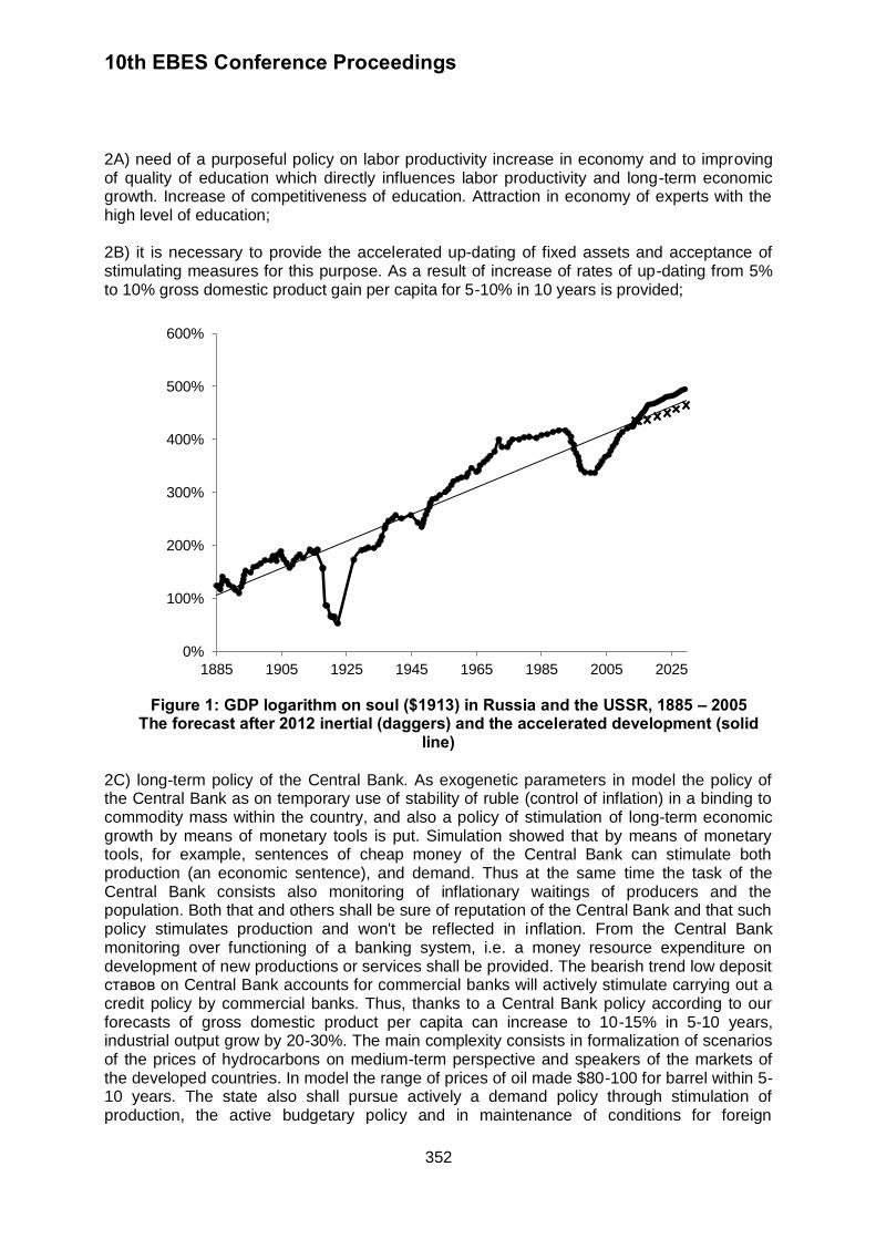
10th EBES Conference Proceedings
352
2A) need of a purposeful policy on labor productivity increase in economy and to improving of quality of education which directly influences labor productivity and long-term economic growth. Increase of competitiveness of education. Attraction in economy of experts with the high level of education; 2B) it is necessary to provide the accelerated up-dating of fixed assets and acceptance of stimulating measures for this purpose. As a result of increase of rates of up-dating from 5% to 10% gross domestic product gain per capita for 5-10% in 10 years is provided;
Figure 1: GDP logarithm on soul ($1913) in Russia and the USSR, 1885 – 2005
The forecast after 2012 inertial (daggers) and the accelerated development (solid line)
2C) long-term policy of the Central Bank. As exogenetic parameters in model the policy of the Central Bank as on temporary use of stability of ruble (control of inflation) in a binding to commodity mass within the country, and also a policy of stimulation of long-term economic growth by means of monetary tools is put. Simulation showed that by means of monetary tools, for example, sentences of cheap money of the Central Bank can stimulate both production (an economic sentence), and demand. Thus at the same time the task of the Central Bank consists also monitoring of inflationary waitings of producers and the population. Both that and others shall be sure of reputation of the Central Bank and that such policy stimulates production and won't be reflected in inflation. From the Central Bank monitoring over functioning of a banking system, i.e. a money resource expenditure on development of new productions or services shall be provided. The bearish trend low deposit ставов on Central Bank accounts for commercial banks will actively stimulate carrying out a credit policy by commercial banks. Thus, thanks to a Central Bank policy according to our forecasts of gross domestic product per capita can increase to 10-15% in 5-10 years, industrial output grow by 20-30%. The main complexity consists in formalization of scenarios of the prices of hydrocarbons on medium-term perspective and speakers of the markets of the developed countries. In model the range of prices of oil made $80-100 for barrel within 5-10 years. The state also shall pursue actively a demand policy through stimulation of production, the active budgetary policy and in maintenance of conditions for foreign
0%
100%
200%
300%
400%
500%
600%
1885 1905 1925 1945 1965 1985 2005 2025
10th EBES Conference Proceedings
353
investments. In case of the active monetary policy of the Central Bank on stimulation of production reduction of an oil and gas component of the budget from the current 40% to 30-35% is possible. 2D) need of increase of efficiency of the state structures. The policy of the Central Bank and the state in the field of education can be leveled insufficiently dynamic and operation of other state structures. 4. CONCLUSION From line items of global simulation methods of creation of scenarios of dynamics of economic systems, formations of classes of similar systems with determination of factors which are indicators of similarity (closeness) are developed. Causes and effect relationships of influence of factors of economic growth and level of their correlation decide on scenarios of dynamics of macroeconomic indexes: Gross domestic product and gross domestic product per capita. Macroeconomic indexes are considered as the indicators reflecting a level of development of economy and welfare of the countries. In case of creation of scenarios of dynamics the criterion of stability of growth of economy is defined. Communication between the listed indexes and depth of the subsequent economic recessions is considered. Attempt to define the periods and depth of business cycles of macroindexes becomes. The following tasks are for this purpose decided:
1) models of the analysis of the heterogeneous economic data inherent in different time slots and regions with the subsequent creation of scenarios speakers of development of the considered countries are constructed. The constructed dependences add ontology of the known formalized economic laws and allow to carry out the correlation analysis between the received results;
2) recommendations about adjustment of proportions in economy structure which within the models of hypotheses accepted in case of creation carry in long-term perspective to increase in labor productivity in economy and to long-term economic growth are formalized;
3) the range of compositions of models is constructed, the pacing factors influencing dynamics of difficult systems are defined;
4) causes and effect relationships between economic indexes (factors) and dynamics of economic growth are defined;
5) the qualifier of the countries on similarity of dynamics of economic development is constructed and factors of economic growth of these countries are revealed;
6) for Russia within the offered model correlation analysis between the general factor labor productivity (one of factors of economic growth) and rate of economic growth is carried out.
Factors and methods of adjustment of dynamics of economic systems are provided. Historical aspects of the reasons and the principles of formation of the factors influencing dynamics of economic systems are analyzed. The used interdisciplinary approach allows to work out new methods to creation of decision making support systems and timely to adjust dynamics of difficult systems and processes proceeding in them (Chmieliauskas et al. 2012, Britkov et al. 2011). REFERENCES Britkov, V.B. and Boulytchev, A.V., 2010. Methods of the analysis of great information volumes. Information technology and computing systems, 1, pp.36-44.

10th EBES Conference Proceedings
354
Britkov, V. and Gelovani, V., 2003. Global modeling. Global studies encyclopedia. Moscow: Raduga Publishers. Britkov, V., Bus, J., and Lehmann, A., 2011. Technology trends and threats. In: The quest for cyber peace - Collection of works of International Telecommunication Union & World Federation of Scientists. Geneva: International Telecommunication Union, pp.31-42, [online] Available at: <http://www.itu.int/dms_pub/itu-s/opb/gen/S-GEN-WFS.01-1-2011-PDF-E.pdf> [Accessed 01 March 2011]. Boulytchev, A.V. and Britkov, V.B., 2011. Research of dynamics of macrosystems on the basis of methodology Data Mining. All-Russia scientific conference collection of works "The System analysis and semiotics modeling SASM – 2011", pp. 56-60. Chmieliauskas, A., Chappin, E., Davis, C., Nikolic, I., and Dijkema, G., 2012. New methods for analysis of systems-of-systems and policy: the power of systems theory, crowd sourcing and data management. In: A.V. Gheorghe, ed. System of Systems. In Tech. pp.77-98. Emelyanov, S.V., Afanasiev, A.P., Grinberg Y.R., Krivtsov V.E., Peltsverger B.V., Sukhoroslov O.V., Taylor R.G., and Voloshinov V.V., 2005. Distributed computing and its applications. Bristol: Felicity Press. Markevich, A. and Harrison, M., 2011. Great war, civil war, and recovery: Russia’s national income, 1913 to 1928. Journal of Economic History, 71(3), pp.672-703.
10th EBES Conference Proceedings 23 - 25 May, 2013. NIPPON HOTEL, ISTANBUL, TURKEY ISBN: 978-605-64002-1-6. WEBSITE: www.ebesweb.org
355
SOVEREIGN WEALTH FUND INVESTMENTS IN THE BANKING INDUSTRY
ANDERLONI LUISA
Department of Economics, Management and Quantitative Methods University of Milan
Italy [email protected]
VANDONE DANIELA
Department of Economics, Management and Quantitative Methods University of Milan
Italy [email protected]
Abstract: This paper aims to investigate the financial impact of Sovereign Wealth Fund
(SWF) investments in banks around the 2008 financial crisis. SWFs have gained great attention because of various concerns: their large size, lack of transparency, and, in principle, the potentially politicized nature of sovereign fund investments. Indeed SWFs disproportionately favor financial companies and during the crisis have become dominant players, providing significant capital to large banks in Europe and the US. Many arguments have been put forth regarding the potential positive and negative effects of SWF investments on global financial markets and on targeted companies. This paper, based on a hand collected database, aims to shed a light on the impact on financial performance (stock prices) and on economic performance (various ratios and growth rates) of SWF investments in banks. We compare the performance of SWF-backed banks with a sample of non- SWF-backed in three time periods (2004-2006, 2007-2008 and 2009-2011) in order to verify the different hypotheses explaining superior or lower performance. This empirical study contributes to the academic literature that seeks to analyze the role of corporate governance structures on banks’ performance. Keywords: Sovereign Wealth Funds, Bank Profitability, Capital and Ownership Structure 1. INTRODUCTION During the financial crisis triggered by the subprime crisis, Sovereign wealth funds (SWFs) emerged as a new and important class of institutional investors both able to provide large amounts of funds to the market and to make large investments in the financial industry worldwide. SWF investments are not a new phenomenon as many of the largest funds have invested around the world for decades; however, they attracted little attention until recent years. Indeed, in the last few years their number has increased, especially with the establishment of new entities from emerging economies. Moreover, they have shown strong growth in their size, with forecasts of further growth. The growth of the scale of SWF investments, and consequently the perception of the potential influence they may have, gave rise to concerns about the SWFs’ role and their implications. Media and popular press in western countries echoed these fears, often viewing SWFs as perilous investors. The matter at issue includes the following. First, the implication of wealth redistribution from private to public hands and a back-tracking from privatization. Second, the threat to national security as a result of the ownership by foreign governments
10th EBES Conference Proceedings
356
and concerns linked to the risk that SWFs may fleece the target firm’s assets or transfer its know-how out of the country. Third, risks of global financial markets’ stability as sudden portfolio adjustments may occur, and risks of distortion of asset prices and destabilization of financial markets and of the global economy if their investments are motivated by political rather than economic considerations. The traditional opaqueness concerning the SWF’s portfolio objectives and activity reinforced these concerns1 and provoked intense debate2. Concerns over political motivations which can drive the SWF investment/disinvestment decisions provided an excuse for calling for protectionist policy measures discouraging foreign investments. In general, the phenomenon reflects a redistribution of international wealth from traditional industrial countries to new emerging inexperienced countries which play no part in the management of the international financial systems and to countries where governments own an important share of this new wealth. Furthermore, what emerged is that, despite their importance and, above all, their expected future growth, very little was known empirically about them. A stream of studies and research was promptly produced. Theory and evidence clearly suggested that concerns about the political motives of SWFs were substantially unfounded. Our paper pursues three objectives. First, to analyze the development path of SWFs’ investments, with a specific focus on the banking sector, over the few years since the phenomenon came to light. Compared with the investments already made known in mid 2000, we wonder if they have been kept, have been withdrawn or have been further developed. Second, to evaluate the operating and financial performance of banks backed by SWFs. Did SWFs invest in banks which performed brilliantly before the crisis? How did banks perform during the crisis? In other words, is there general evidence that SWFs provided resources to distressed banks? And, what were the trends in the period that followed? Furthermore, did banks backed by SWFs show a more significant strengthening of the capital than those which did not have this injection of capital? Third, to investigate the role of SWFs in banks’ corporate governance. Which observations emerge about the possible appointments of representatives on the Boards? This paper contributes to shedding light to a phenomenon so far understudied, albeit of growing importance and with relevant implications for both market participants and regulators. The empirical analysis is based on data from 27 banks; these banks are spread throughout the world and represent the entire population of banks with a SWF participation of more than 2% of their capital. The paper is structured as follows: section 2 provides an overview of the recent developments of the SWFs’ sector, in section 3 we review relevant theoretical perspectives and the earlier studies on SWFs. Our data sources and methodology are described in section 4. Section 5 presents the results. The final section concludes the paper.
1 Truman (2008) illustrated in great detail these concerns grouping them in five points. Various official initiatives
(from G-8/G-7, IMF, US Treasury, the Commission of the European Communities) took place calling for best practices for SWFs in the areas of institutional structure, risk management, transparency and accountability. 2 As of fact some deals were blocked or the original investment reduced: Kuwait Investment Office – British
Petroleum in 1987, Government of Dubai – P&O in 2006.
10th EBES Conference Proceedings
357
2. RECENT DEVELOPMENTS OF THE SWF SECTOR SWFs are a heterogeneous phenomenon and so far there is no consensus on a common definition of SWFs3. If they have existed since at least the 1950s – the set up of the Kuwait Investment Office dates back to 1953 – the bulk of them were created in the last 10-15 years and the amount of assets under management has grown suddenly reaching a volume of asset under management estimated at about $ 5,000 billion in the first quarter of 2012 from about $ 500 billion in 2005. The sector is highly concentrated: the first 5 largest funds - out of the 62 ranked by the Sovereign Wealth Fund Institute – are estimated to manage about 56.6 percent of the total asset under management by SWFs and the first 10 are estimated to reach a share of about 80 percent. On the top of the ranking we find funds newly set up funds such as the China Investment Corporation - established in 2007 - and the Russian National Welfare fund - set up in 2008 - together with the historical ones, such as Abu Dhabi from UAE which stands at first place and the Kuwait Investment Authority now ranking at sixth place. Table 1 provides some information about the 25 largest SWFs. Among the recent trends we should mention the establishment of new funds: since 2005, at least 20 sovereign wealth funds have been created. Their growth has also been caused by rising commodity prices, especially oil and gas, mainly between 2003-2008, but not only: in one year – in 2011 five new funds were created. Another interesting trend is the development of investment vehicles that are owned and controlled by sovereign wealth funds. Although these vehicles provide greater flexibility for SWFs, they further reduce transparency.
As previously mentioned, in recent years a large share of investments has been channeled into the financial sector, as defined in broad terms, i.e. including not only banks, but also financial firms, asset management firms, financial brokers, insurance companies and stock exchanges. It is worth mentioning the investment in the latter. On one hand, it is a widespread phenomenon which refers to many among the more important stock exchanges of western countries, involves various SWFs and the shares undertaken are large. On the other hand, it refers to investments in infrastructures of vital importance for the economic and financial activity of a country.
Estimates from the Sovereign Wealth Funds Institute indicate that in the period March 2007-April 2008 total cash injection from Sovereign Wealth Funds in the large international banks was nearly $ 45,000 million both in common stock and - to a large extent - in new convertible units that can be converted – or are mandatorily converted - into equity at a future date.
3 According to the historiography this term has been coined by Razanov recently, in 2005.
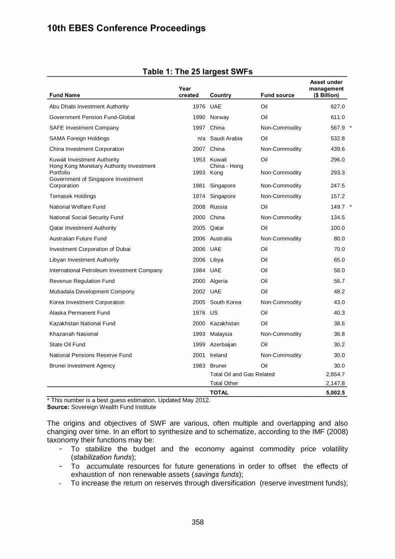
10th EBES Conference Proceedings
358
Table 1: The 25 largest SWFs
Fund Name Year created Country Fund source
Asset under management
($ Billion)
Abu Dhabi Investment Authority 1976 UAE Oil 627.0
Government Pension Fund-Global 1990 Norway Oil 611.0
SAFE Investment Company 1997 China Non-Commodity 567.9 *
SAMA Foreign Holdings n/a Saudi Arabia Oil 532.8
China Investment Corporation 2007 China Non-Commodity 439.6
Kuwait Investment Authority 1953 Kuwait Oil 296.0 Hong Kong Monetary Authority Investment Portfolio 1993
China - Hong Kong Non-Commodity 293.3
Government of Singapore Investment Corporation 1981 Singapore Non-Commodity 247.5
Temasek Holdings 1974 Singapore Non-Commodity 157.2
National Welfare Fund 2008 Russia Oil 149.7 *
National Social Security Fund 2000 China Non-Commodity 134.5
Qatar Investment Authority 2005 Qatar Oil 100.0
Australian Future Fund 2006 Australia Non-Commodity 80.0
Investment Corporation of Dubai 2006 UAE Oil 70.0
Libyan Investment Authority 2006 Libya Oil 65.0
International Petroleum Investment Company 1984 UAE Oil 58.0
Revenue Regulation Fund 2000 Algeria Oil 56.7
Mubadala Development Compony 2002 UAE Oil 48.2
Korea Investment Corporation 2005 South Korea Non-Commodity 43.0
Alaska Permanent Fund 1976 US Oil 40.3
Kazakhstan National Fund 2000 Kazakhstan Oil 38.6
Khazanah Nasional 1993 Malaysia Non-Commodity 36.8
State Oil Fund 1999 Azerbaijan Oil 30.2
National Pensions Reserve Fund 2001 Ireland Non-Commodity 30.0
Brunei Investment Agency 1983 Brunei Oil 30.0
Total Oil and Gas Related 2,854.7
Total Other 2,147.8
TOTAL 5,002.5
* This number is a best guess estimation. Updated May 2012. Source: Sovereign Wealth Fund Institute The origins and objectives of SWF are various, often multiple and overlapping and also changing over time. In an effort to synthesize and to schematize, according to the IMF (2008) taxonomy their functions may be:
- To stabilize the budget and the economy against commodity price volatility (stabilization funds);
- To accumulate resources for future generations in order to offset the effects of exhaustion of non renewable assets (savings funds);
- To increase the return on reserves through diversification (reserve investment funds);

10th EBES Conference Proceedings
359
- To create a pool of resources in order to fund socio-economic projects or to sustain the growth of domestic strategic companies or to help stabilize domestic firms (development funds); 4
- To create a pool of resources to face contingent unspecified pension liabilities on the government’s balance sheet, generally investing parts of the large surplus generated by commodities (usually oil) though taxes from companies or payments of licenses fees (contingent pension reserve funds).
Indeed, missions and objectives of each fund may evolve over time – generally from stabilization to savings – and contemporaneously also investment horizons, liquidity needs and asset allocation criteria are modified. This is a sector which is evolving over time and it seems interesting to study the trends. 3. LITERATURE REVIEW Research questions that fed the recent literature on SWFs can be, in our opinion, grouped into four areas; it is worth mentioning that they were initially formulated in a context of lack of knowledge and of substantial mistrust and fear about the role played by this new class of institutional investors. The first group of research questions are as follows: What are the SWFs and what are their objectives? How do they invest and which asset allocation models do they adopt? What are their organisational models, i.e. do they manage their portfolios internally or do they delegate the job to external professional managers? Furthermore: what is the size of their investments? In this stream, models have been suggested to answer the question regarding the appropriate models to estimate the development patterns and the liquidity needs of the sector. The second group includes analyses focusing on the macroeconomic implications of SWFs activity. The questions refer, primarily, to the stability of the financial systems, but also to the economies both of countries receiving funding from SWFs and of the same investing countries. In the third group the focus is on the microeconomic implications of SWF investments on targeted firms, and more precisely on listed companies both in the short and in the long term. In the last group we find questions relative to corporate governance behaviour, geopolitical concerns, and transparency matters. 3.1. The sector and its trends In the first stream of literature the most influential works are IMF (2008), the Sovereign Wealth Fund Institute analysis and research and various reports of Enrico Mattei Foundation-Monitor Group which constantly monitor investments made by SWFs, identify the trends and strategies, and provide information about the sector structure. The SWFs invest, in different proportions, in bonds issued by the Treasuries of Sovereign States and international organisations, in real estate and equities, both of listed companies and in placements of private equity, to a lesser extent in hedge funds and commodities and,
4 In this category we find the Strategic Development Sovereign Wealth Fund (SDSWF) whose mission is to
promote national economic or development goals and whose investments are mainly in domestic strategic companies. The newest is the Italian Strategic Fund launched in 2011 on the model of the French Strategic Investment Fund.
10th EBES Conference Proceedings
360
more recently, even in project finance operations. A new trend, with only a few cases and limited amounts, is the use of leverage. The SWFs often invest in the primary markets, so far providing capital injections in the issuing firms. The recent investments in the banking sector have also been made, to a large extent, by private placements of convertible units, as they were aimed at helping the recapitalization of banks suffering from losses and depreciations. As previously said, the opaqueness that still characterizes the way some SWFs operate make their analysis very difficult. Thus, studies and research have mainly focused on investments in listed companies. In this area, the SWFs seem to prefer to invest in large companies, of the growth type, with proven profitability, levered and headquartered in OECD countries (Bortolotti et al. 2010, Fernandes, 2009, Kotter and Lel, 2011).
Bortolotti et al. (2010) also find that SWFs generally purchase minority stakes directly from
target companies, roughly half of which are unlisted and very frequently are based in the fund’s home country. Furthermore financial companies investments are disproportionately favoured by SWFs. Fernandes (2009) also documents that SWFs invest much less in high-tech firms, i.e. with a high level of R&D assets. This is in contrast to the fear of investments in western corporations aimed at gathering know-how. On the contrary, Kotter and Lel (2011) observe that in general SWFs target large firms that are poorly performing, financially-distressed, and cash-constrained. They also find that transparent SWFs are more likely to prefer firms facing financial difficulties than opaque ones. The high degree of SWF investments in distressed companies was also pointed out by Chhaochharia and Laeven (2008a). Bernstein et al. (2009) analyzed SWFs’ private equity investment strategies and
their relationship to the funds’ organizational structures. They report that the funds seem to adopt a trend following pattern since they tend to invest at home when domestic equity prices are higher, and tend to invest abroad when foreign prices are higher. In addition, as for the governance model, SWFs in which politicians are involved are more likely to invest in the domestic market than those in which external managers are involved. The latter more frequently invest at significantly lower Price/Earning ratios when investing at home and at higher Price/Earning ratios when investing abroad. Chhaochharia and Laeven (2008b) also analysed the asset allocation pattern of SWFs and find that SWFs are more likely to invest in countries that share similar cultural features, especially religion, indicating that SWF investments are biased towards the familiar. Indeed this cultural bias is also common to other institutional investors, but for SWFs it seems more pronounced. In addition, the authors point out that this cultural bias gradually disappears following numerous investments in the same country. Avendano and Santiso (2009) deal with the comparison between SWFs’ investments and other institutional investors, i.e. mutual funds: comparing the geographical/sector allocation and the target firms’ profile. Their results suggest that SWFs show more similarities than differences compared to other institutional investors. This reinforces the hypothesis that their asset allocation strategies are driven by financial objectives. Finally, Raymond (2010) qualifies SWFs as “domestic investors of last resort” during the 2008 crisis and discusses the role of SWFs as insurance funds against major crises pointing out that not all SWFs are backed by a large pool of assets, including safe liquid assets. Studies on SWF investments during the subprime crisis, show that investment flows are disproportionately channelled towards financial institutions, and in regional terms, towards the US. Thus SWFs might have taken the advantage of the low prices to invest in an attractive but ailing industry. This might also have produced reputational benefits. Generally,
10th EBES Conference Proceedings
361
scholars agree that SWFs acted like passive shareholders and adopted a long term investment strategy. 3.2. Macroeconomic implications In this area, we are interested especially in studies investigating the question of whether SWFs have a potential destabilizing force. Sun and Hesse (2009), using an event study approach, analyse the impact of SWFs on financial stability. It is worth mentioning the results concerning the divestment effect: the reactions on equity markets, as measured by abnormal return behaviour, in developed economies and emerging economies, are generally statistically insignificant, while - in line with the results of other studies commented upon below - SWF investments produce a positive impact. Knill et al. (2012) also address the question of whether the investment of SWFs mitigates risks or is potentially destabilizing, focusing on the effects of SWFs on volatility and the return to risk relation. They find that SWF investments are followed by a decline in the return of the target firms. At the same time, the volatility of the target firms decreases, but not enough to compensate investors for the risk as established by the capital asset pricing model. Beck and Fidora (2008) analyse the impact of SWFs on global financial markets by simulating the potential impact of a transfer of traditional foreign exchange reserve to SWFs on global capital flows. The results of their simulation show that if SWFs behave like CAPM-type investors there will be capital outflows from rich countries to less wealthy economies, especially from the United States and the Euro area to Japan and emerging markets. 3.3. Microeconomic implications From our standpoint the most interesting stream of research focuses on the impact of SWF investments on target firms’ performance both in the short and in the long term. The analyses on the short term are focused on the stock price reaction to the announcement of an SWF investment. In principle, a positive reaction denotes that the investments convey positive information to the market, such as liquidity and capital provision, screening and monitoring activities, while negative reactions should confirm concerns about the previously mentioned risks The researchers find that the stock price reaction to SWF investment is generally positive, ranging from about 0.5% to about 2.5%5, depending on the sample, metrics and geographical contexts used (Bortolotti et al. 2010, Kotter and Lel, 2008, 2011, Dewenter et al. 2010, Chhaochharia and Laeven, 2008a, Raymond 2009, Knill et al. 2009). However it is worth mentioning that each paper has a slightly different focus. Thus SWF investments seem to send a positive signal to market participants about the future performance of target firms, providing a certification of the firm’s long term economic viability. Furthermore, Dewenter et al. (2010) suggest that these investments also create expectations about
valuable monitoring or lobbying activities conducted by the SWFs. Kotter and Lel (2011) notice that the positive market reaction to SWF acquisition announcements is similar to that of investments by hedge funds and private equity funds. Further analysis shows that firms targeted by SWFs with higher disclosure standard (including transparency, structure, governance and behaviour) show higher abnormal returns. In particular, “transparency” and “governance” have a positive and statistically
5 Raymond (2009) finds that, for his/her sample, the abnormal rate of return is around 6% and excluding two
outliers, it drops to 3,85%. However the analysis is based on a sample limited to acquisitions made during the subprime crisis.

10th EBES Conference Proceedings
362
significant effect on the magnitude of the stock price impact. Part of this positive short term effect could be explained by SWF investments in distressed companies (Chhaochharia and Laeven, 2008a and Kotter and Lel, 2011). The above mentioned studies generally use large samples which involve investments in several sectors and in different countries, including domestic investments or investments in geographically and culturally close countries. It is common that authors highlight the relevant share of investments in the broad financial sector. To the best of our knowledge, however, only two studies have focused on investments in the banking sector. Kern (2008) focuses the analysis on investments in international banks during the 2007-2008 financial crisis. The SWFs’ impact on bank share price is negligible on the whole, and even in cases where the impact of the event can be identified (in terms of volatilities and abnormal return), the direction of the impact is not homogeneous6. According to the author, it would be an exaggeration to consider that SWF commitments can fundamentally alter market sentiments in fragile market conditions. Moreover Raymond (2009) tests the effect of the SWF acquisitions on a sub-range of events occurring between July and April 20087 and finds a positive daily abnormal price change on the day of the announcement of the investment by a SWF, but this change is weaker than that seen in the study using the complete sample. Furthermore, this very temporary positive effect is too weak to remain statistically significant when it is aggregated in cumulated abnormal price changes. Then, analysing the reaction to divestments, the results of different studies are controversial. According to Dewenter et al. (2010) the pattern is reversed and the effect is negative,
findings which are in line with those of Kotter and Lel (2008) based on a very small sample of events. According to Beck and Fidora (2008) there would be no negative effects, but it should be noted that their analysis is limited to the Norwegian Government Pension Fund – Global whose decisions are well known to have an explicit strategy of minimal market impact. Controversial results are also found in literature with reference to long run performance. According to Bortolotti et al. (2010) and Knill et al. (2009) the vast majority of SWF investments are followed by firm performance deterioration. Bortolotti et al. (2008) interpret
the lower long run performance through the Constrained Foreign Investor Hypothesis which predicts that foreign investors, especially when large and promoted by sovereign states, can not perform a monitoring function appropriately, due to the concern of avoiding the risk of antagonizing the local management. Kotter and Lel (2011) observe that in the medium term (i.e. in the three year period following the SWF investment) the target firms do not undergo any robust and statistically significant change in their profitability, growth, investment, and corporate governance structure. Their evidence also implies that SWF investments do not compromise firm value. Their results show that SWFs do not improve firm value in the long run, suggesting that SWFs are not commonly active shareholders. Instead Dewenter et al. (2010) find that, for their full sample, the mean and the median adjusted returns are negative over the one year period following the investment, but mixed evidence of significant positive returns was found over three and five year periods. Similarly, Fernandes (2009) shows that overall operational performance – measured according to
6 On the one hand, the follow up investment in Citigroup and the investments in Merrill Lynch, Morgan Stanley
and Barclays seem to have pushed cumulative returns upwards. On the other hand, cumulative returns on the stocks of Deutsche Bank, UBS and Credit Suisse either remained flat or in fact started to decline. 7 These events include investments by SWFs in Citigroup, UBS, Morgan Stanley, Merrill Lynch and Credit Suisse.
10th EBES Conference Proceedings
363
different metrics – improves over different periods before and after SWF investments for stake acquisitions larger than 1%. Bernstein et al. (2009) find significant performance
differences for SWF home versus cross border investments. Finally, considering the investments in the financial sector, it is worth noting that Knill et al. (2009) find that financial targets have better long-run returns than non-financial targets. 3.4. Governance, transparency and geopolitical implications In this area, the research is mainly qualitative. The most noteworthy study is Clark and Monk (2009) from Oxford University, who conducted an interesting survey about experts’ experience of work with SWFs and their opinion on operations and behaviour of this class of institutional investors. Other studies are purely theoretical papers, such as those from OECD (2009) concerning the policies of receiving countries or that of Drezner (2010) dealing with various political concerns raised, in principle, by SWF activity. Furthermore, various single case-studies have been presented. Among empirical papers, we have to mention again Bortolotti et al. (2010) who investigate whether SWFs appoint their representatives as
members of the Board of Directors and analyses the relationship between performance and degree of involvement of the SWF. When investments made by the Norwegian fund are excluded, the results show that SWFs obtained board representation in 28.8% of cases. Significant differences are found among funds: Khazanah and Temasek obtained board seats far more often than other funds, whereas ADIA, Kuwait Investment Authority and Qatar Investment Authority very rarely got them. A further difference concerns domestic and foreign investments: SWFs are much more likely to gain seats in domestic and regional investments than in foreign investments, especially in OECD countries. In particular, there are no cases in the UK and very few in the US. These results suggest that SWFs are not keen to exercise effective corporate governance over their foreign investments, but they are much more inclined to do so domestically. Often board seats are to a large extent obtained through SWF-subsidiary investments. This might be because SWFs make the conscious and rational decision to channel more sensitive foreign investments into low profile subsidiaries instead of making them directly. According to the authors, the results support the above mentioned Constrained Foreign Investor Hypothesis which states that “as state-owned investment funds from largely non-democratic countries, these funds are politically constrained from exercising effective discipline of target firm managements – especially in the United States, Britain and continental Europe”8. Using regression analysis, they find greater underperformance when SWFs have closer involvement, indicating that indeed they fail to perform the monitoring role usually associated with large shareholders. SWFs therefore do not appear to really monitors the companies and do not lead to increased firm value. By contrast, Dewenter et al. (2010) find that SWFs have often closer involvement and play
an active role in their target firms. Considering a series of events representative of SWF monitoring or influence9, their results indicate that at least one of these events occurs in just over half of the SWF purchase announcements. In addition, they show that this post-investment activity is significantly related to the target’s long run return, In particular networking activities are associated with significantly higher returns in cross border
8 The analysis is done by isolating the case of the Norwegian fund that never acquires significant amounts of
outstanding shares and never takes any board seats. 9 These include the assumption of directorship by SWF representatives, senior management turnover at the
target firm, target firm business deals with firm related to the SWF, and favourable or unfavourable government regulatory decisions affecting the target firm.
10th EBES Conference Proceedings
364
investments, but not in domestic investments. By contrast, Kotter and Lel (2008) examine post-investment influence by comparing post-investment performance and CEO turnover in a sample of SWF targets and in a control group. They find no significant differences between target and control samples and conclude that SWFs are passive investors. Adopting a different perspective of governance, i.e. focusing on SWFs management and analysing direct private equity strategies, Bernstein et al. (2009) find that when politicians are
actively involved in establishing SWF investment policies, funds have a much higher probability of investing at home than abroad, and this influence reduces their performance. Finally Kotter and Lel (2008 and 2011) document that the degree of transparency of SWF activity is an important factor in explaining market reactions, while Knill et al. (2009) investigate whether bilateral political relations play a role in SWF investment decisions. They, contrary to literature predictions, find that SWFs are more likely to invest in countries with which they have relatively weaker political relations. Moreover, by using a model which separates the two choices in SWF investment decisions (choice of country and investment amount) they find the former is an important factor, while the latter is less influential. 4. EMPIRICAL DESIGN AND SAMPLE DATA To answer our research questions we mapped the SWF investments in the banking sector in the period 2005-2011. We started with the European countries and the US. Later on we added other investments in the banking sector worldwide. Our data collection follows a three-step procedure. As a first step, we used the Bureau Van Dijk Bankscope database to find the largest 25 banks in each European country and the US. As a second step, we gathered the ownership information for these banks from many different sources. We started with the Bankscope (sections “deals and news” and “ownership”) and Zephir M&A databases searching for the SWF names and their well-known vehicles, then we used each individual bank’ annual reports for the years 2005-2011 and corporate governance information to find out the investments made by SWFs, considering the entities included in the list of the Sovereign Wealth Fund Institute and their vehicles. We decided not to consider the investment made by Norway’s Government Pension Fund-Global as it is well known as a passively investor of small amounts of capital through open market stock purchases, adopting a sort of equity index replication strategy. In the final step, we also checked information provided by each fund - when available - by the SWF Institute web site, which contains information about some funds, by various reports of Monitor Group-FEEM, and by the Bureau Van Dijk-Orbis database searching for the SWF name, “subsidiary” section. In addition, we checked holding information from mandatory
filings with national regulatory agencies. Previous studies were also particularly useful in this phase10. At the end of this procedure we found 20 banks whose shareholders included SWFs, excluding domestic investments11 and those investments in banks with common stocks not listed on Stock Exchanges, i.e. for which Datastream does not include listed common stocks. This allowed us to achieve an initial result with our analysis, answering the question about where SWFs invest in the US and Europe. Due to the numerous very small shares of ownership (less than 1%) not mentioned in most of the annual reports and corporate governance reports, we restricted our sample to banks where the investment was higher than 2%. This research resulted in a total of 13 banks. For
10
See ECB (2008), 11
This means that various investments mainly in China, Indonesia and Ireland have not been considered in our analysis.
10th EBES Conference Proceedings
365
these banks we also researched the composition of the board of directors in order to verify whether SWFs were passive investors or whether they expected seats and an active role in the corporate governance. Then we added the other worldwide cross border investments in the banking sector, on the conditions that they had publicly-traded stocks and the SWF investments were greater than 2%. In order to gather data for these investments, we proceeded in reverse order: from various reports, individual fund’s web pages and databases, to annual reports of each bank and related information provided by Bankscope and Zephir databases. In total we found 27 banks worldwide, listed on the Stock Exchanges, where a SWF invested at least 2% of capital. Due to the very limited dimension of our sample, we decided to proceed with only descriptive statistic tools. We performed - on the one hand - the analysis on different measures of banks’ operating performances and we use Return on equity (ROE), Return on asset (ROA) and Variation of total equity as an indicator of capital reinforcement and – on the other hand – the analysis of financial performance on stock markets. We were interested in verifying whether the banks backed by SWFs performed better or worse or similarly compared to similar banks which were not the target of SWF investments. As for the time period considered, on the operational side we used a large window before the sub-prime crisis - from 2000 - and the two years following it, for which data are available. The data were analysed year by year, in addition averages were used for sub-periods. On the financial side, we used different periods of analysis: the first includes three years before the sub-prime crisis (2004-2006), the second is that of the acute crisis (2007-2008) and the last, symmetrically, includes the three years post crisis (2009-2011). In order to evaluate the stock performance we examined the Compound return, ie. the Compound Annual Growth Rate –CAGR and the Compound Adjusted Annual Growth Rate –CAAGR
(1) In addition, in order to evaluate the capital adequacy position, we used the “Tier 1 Regulatory Capital Ratio” and the “Regulatory Total Capital Ratio” provided by the Bureau Van Dijk
Bankscope database for each bank. We selected a control sample of banks that were not targets of SWF investments, but similar in terms of country of incorporation (or, in very few cases, comparable in terms of their international position in Europe), dimension (total asset) and specialisation. Therefore we compared the performances of SWF-backed banks and those of non SWF-backed banks. The aim of this analysis is:
- to verify whether SWF target banks are banks with a track record of success, i.e. with superior operational and financial performance before the crisis,
- to verify the commonly held idea that SWFs acted as “saviours” of financially distressed financial institutions during the crisis;
- to verify whether the post-crisis performance of the SWF-backed banks are better than that of non SWF-backed banks.
1Value Beginning Price
Value Ending PriceCAGR
1
i
years
i
i
yearsyears
i
i
11
iValue BeginningIndex Market
Value EndingIndex Market
Value Beginning Price
Value Ending PriceCAAGR
10th EBES Conference Proceedings
366
5. EMPIRICAL RESULTS Table 2 provides the country distribution of cross-border SWF investments in the banking sector, the date of the first relevant investment from a SWF and the number of SWFs investing in each bank. As we can notice, more attractive countries are the US, followed by the UK and China (3 banks each), Switzerland and India (2 banks each). Eighteen other countries record only one bank target of SWF investments. The most attractive banks are large banks, at the top or in a high level position in the ranking by dimension of their countries. Regarding the period of investment, we can confirm that the bulk of investments in the US and Europe were made during the sub-prime crisis with a few cases in 2006, whereas in the rest of the world we find some investments before the crisis - in 2003 and 2005- but the vast majority have been made in the last two years or in the current year. Investments have been made mainly by direct purchases - which represent capital infusion for target banks - by private placements of (mandatory) convertible bonds or equity units, paying a fixed annual rate, which is generally very high, as it includes a high risk premium. Shareholdings – both direct purchases of stocks and through the subsequent conversion of bonds or units – are generally minority stakes: starting from our threshold of 2%, they are generally lower than 10%, with, however, some significant exceptions. For the US banks, the threshold of 10% is always observed, in order not to hold the position of Bank Holding Company. Considering the minority stakes, we have to highlight two aspects. Firstly, due to the large dimension of SWF target banks, the amount of resources provided to banks is enormous, thereby keeping the banking sector12 one of the most attractive sectors for SWFs. Secondly, especially in countries such as the UK and the US where the dominant ownership model is that of public companies, the above mentioned minority stakes become important: with reference to the 9 European banks in which SWFs have invested, we can count 3 cases in which a SWF is/has been the first shareholder, 3 cases in which it takes the second place, 2 additional cases in which it ranks third and 1 which comes fourth. In conclusion, investments appear as minority stakes but, in relative terms, they are considerable undertakings. In the light of these relative positions, it seems interesting to verify the role played by the SWFs in the corporate governance. As for the role played by the SWFs in the corporate governance, out of the 9 cases of European banks targeted by SWFs, we find 4 cases of SWF representatives on the Boards, including 1 Vice president, 2 cases of appointment of members of the Board of directors and 1 case of appointment of 2 members (out of 3) of the supervisory board. It is worth mentioning, however, that none of the above mentioned cases refers to British banks. We can also point out that generally the banks which attract SWF investments are very large banks that occupy the top positions in the rankings by dimension in their countries. This is especially true of the US, Europe and China.
12
Indeed the banking sector is often considered in broad terms including asset management firms and Stock Exchanges.
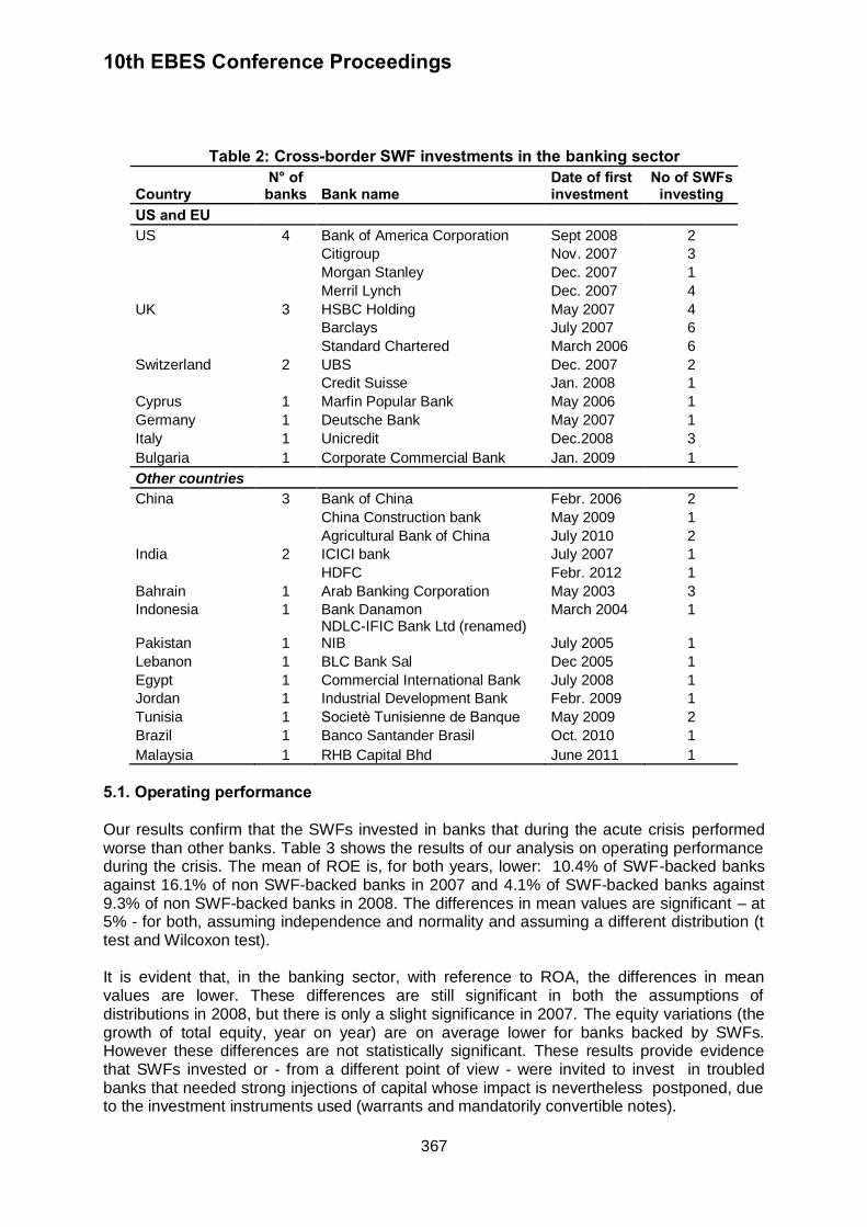
10th EBES Conference Proceedings
367
Table 2: Cross-border SWF investments in the banking sector
Country N° of banks Bank name
Date of first investment
No of SWFs investing
US and EU
US 4 Bank of America Corporation Sept 2008 2
Citigroup Nov. 2007 3
Morgan Stanley Dec. 2007 1
Merril Lynch Dec. 2007 4
UK 3 HSBC Holding May 2007 4
Barclays July 2007 6
Standard Chartered March 2006 6
Switzerland 2 UBS Dec. 2007 2
Credit Suisse Jan. 2008 1
Cyprus 1 Marfin Popular Bank May 2006 1
Germany 1 Deutsche Bank May 2007 1
Italy 1 Unicredit Dec.2008 3
Bulgaria 1 Corporate Commercial Bank Jan. 2009 1
Other countries
China 3 Bank of China Febr. 2006 2
China Construction bank May 2009 1
Agricultural Bank of China July 2010 2
India 2 ICICI bank July 2007 1
HDFC Febr. 2012 1
Bahrain 1 Arab Banking Corporation May 2003 3
Indonesia 1 Bank Danamon March 2004 1
Pakistan 1 NDLC-IFIC Bank Ltd (renamed) NIB July 2005 1
Lebanon 1 BLC Bank Sal Dec 2005 1
Egypt 1 Commercial International Bank July 2008 1
Jordan 1 Industrial Development Bank Febr. 2009 1
Tunisia 1 Societè Tunisienne de Banque May 2009 2
Brazil 1 Banco Santander Brasil Oct. 2010 1
Malaysia 1 RHB Capital Bhd June 2011 1
5.1. Operating performance Our results confirm that the SWFs invested in banks that during the acute crisis performed worse than other banks. Table 3 shows the results of our analysis on operating performance during the crisis. The mean of ROE is, for both years, lower: 10.4% of SWF-backed banks against 16.1% of non SWF-backed banks in 2007 and 4.1% of SWF-backed banks against 9.3% of non SWF-backed banks in 2008. The differences in mean values are significant – at 5% - for both, assuming independence and normality and assuming a different distribution (t test and Wilcoxon test). It is evident that, in the banking sector, with reference to ROA, the differences in mean values are lower. These differences are still significant in both the assumptions of distributions in 2008, but there is only a slight significance in 2007. The equity variations (the growth of total equity, year on year) are on average lower for banks backed by SWFs. However these differences are not statistically significant. These results provide evidence that SWFs invested or - from a different point of view - were invited to invest in troubled banks that needed strong injections of capital whose impact is nevertheless postponed, due to the investment instruments used (warrants and mandatorily convertible notes).
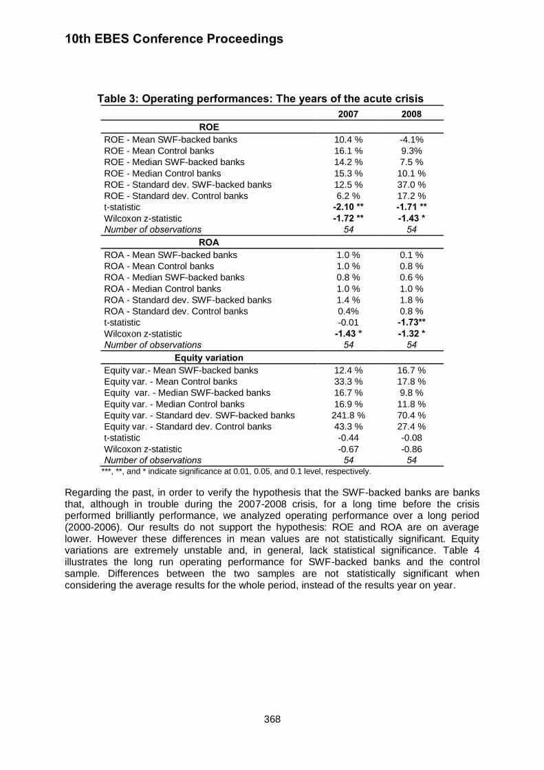
10th EBES Conference Proceedings
368
Table 3: Operating performances: The years of the acute crisis 2007 2008
ROE
ROE - Mean SWF-backed banks 10.4 % -4.1%
ROE - Mean Control banks 16.1 % 9.3%
ROE - Median SWF-backed banks 14.2 % 7.5 %
ROE - Median Control banks 15.3 % 10.1 %
ROE - Standard dev. SWF-backed banks 12.5 % 37.0 %
ROE - Standard dev. Control banks 6.2 % 17.2 %
t-statistic -2.10 ** -1.71 ** Wilcoxon z-statistic -1.72 ** -1.43 * Number of observations 54 54
ROA
ROA - Mean SWF-backed banks 1.0 % 0.1 %
ROA - Mean Control banks 1.0 % 0.8 %
ROA - Median SWF-backed banks 0.8 % 0.6 %
ROA - Median Control banks 1.0 % 1.0 %
ROA - Standard dev. SWF-backed banks 1.4 % 1.8 %
ROA - Standard dev. Control banks 0.4% 0.8 %
t-statistic -0.01 -1.73** Wilcoxon z-statistic -1.43 * -1.32 * Number of observations 54 54
Equity variation
Equity var.- Mean SWF-backed banks 12.4 % 16.7 %
Equity var. - Mean Control banks 33.3 % 17.8 %
Equity var. - Median SWF-backed banks 16.7 % 9.8 %
Equity var. - Median Control banks 16.9 % 11.8 %
Equity var. - Standard dev. SWF-backed banks 241.8 % 70.4 %
Equity var. - Standard dev. Control banks 43.3 % 27.4 %
t-statistic -0.44 -0.08
Wilcoxon z-statistic -0.67 -0.86
Number of observations 54 54 ***, **, and * indicate significance at 0.01, 0.05, and 0.1 level, respectively.
Regarding the past, in order to verify the hypothesis that the SWF-backed banks are banks that, although in trouble during the 2007-2008 crisis, for a long time before the crisis performed brilliantly performance, we analyzed operating performance over a long period (2000-2006). Our results do not support the hypothesis: ROE and ROA are on average lower. However these differences in mean values are not statistically significant. Equity variations are extremely unstable and, in general, lack statistical significance. Table 4 illustrates the long run operating performance for SWF-backed banks and the control sample. Differences between the two samples are not statistically significant when considering the average results for the whole period, instead of the results year on year.
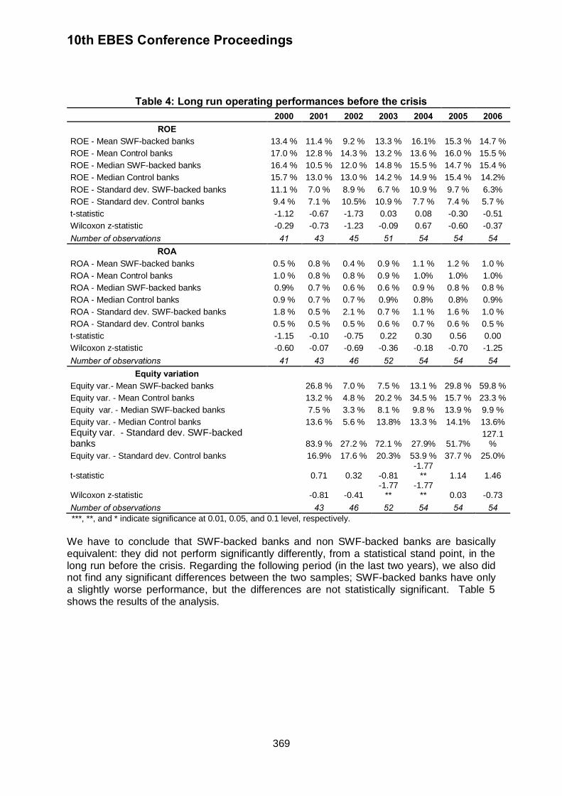
10th EBES Conference Proceedings
369
Table 4: Long run operating performances before the crisis
2000 2001 2002 2003 2004 2005 2006 ROE
ROE - Mean SWF-backed banks 13.4 % 11.4 % 9.2 % 13.3 % 16.1% 15.3 % 14.7 %
ROE - Mean Control banks 17.0 % 12.8 % 14.3 % 13.2 % 13.6 % 16.0 % 15.5 %
ROE - Median SWF-backed banks 16.4 % 10.5 % 12.0 % 14.8 % 15.5 % 14.7 % 15.4 %
ROE - Median Control banks 15.7 % 13.0 % 13.0 % 14.2 % 14.9 % 15.4 % 14.2%
ROE - Standard dev. SWF-backed banks 11.1 % 7.0 % 8.9 % 6.7 % 10.9 % 9.7 % 6.3%
ROE - Standard dev. Control banks 9.4 % 7.1 % 10.5% 10.9 % 7.7 % 7.4 % 5.7 %
t-statistic -1.12 -0.67 -1.73 0.03 0.08 -0.30 -0.51
Wilcoxon z-statistic -0.29 -0.73 -1.23 -0.09 0.67 -0.60 -0.37
Number of observations 41 43 45 51 54 54 54 ROA
ROA - Mean SWF-backed banks 0.5 % 0.8 % 0.4 % 0.9 % 1.1 % 1.2 % 1.0 %
ROA - Mean Control banks 1.0 % 0.8 % 0.8 % 0.9 % 1.0% 1.0% 1.0%
ROA - Median SWF-backed banks 0.9% 0.7 % 0.6 % 0.6 % 0.9 % 0.8 % 0.8 %
ROA - Median Control banks 0.9 % 0.7 % 0.7 % 0.9% 0.8% 0.8% 0.9%
ROA - Standard dev. SWF-backed banks 1.8 % 0.5 % 2.1 % 0.7 % 1.1 % 1.6 % 1.0 %
ROA - Standard dev. Control banks 0.5 % 0.5 % 0.5 % 0.6 % 0.7 % 0.6 % 0.5 %
t-statistic -1.15 -0.10 -0.75 0.22 0.30 0.56 0.00
Wilcoxon z-statistic -0.60 -0.07 -0.69 -0.36 -0.18 -0.70 -1.25
Number of observations 41 43 46 52 54 54 54 Equity variation
Equity var.- Mean SWF-backed banks 26.8 % 7.0 % 7.5 % 13.1 % 29.8 % 59.8 %
Equity var. - Mean Control banks 13.2 % 4.8 % 20.2 % 34.5 % 15.7 % 23.3 %
Equity var. - Median SWF-backed banks 7.5 % 3.3 % 8.1 % 9.8 % 13.9 % 9.9 %
Equity var. - Median Control banks 13.6 % 5.6 % 13.8% 13.3 % 14.1% 13.6%
Equity var. - Standard dev. SWF-backed banks 83.9 % 27.2 % 72.1 % 27.9% 51.7%
127.1 %
Equity var. - Standard dev. Control banks 16.9% 17.6 % 20.3% 53.9 % 37.7 % 25.0%
t-statistic 0.71 0.32 -0.81 -1.77
** 1.14 1.46
Wilcoxon z-statistic -0.81 -0.41 -1.77
** -1.77
** 0.03 -0.73
Number of observations 43 46 52 54 54 54 ***, **, and * indicate significance at 0.01, 0.05, and 0.1 level, respectively.
We have to conclude that SWF-backed banks and non SWF-backed banks are basically equivalent: they did not perform significantly differently, from a statistical stand point, in the long run before the crisis. Regarding the following period (in the last two years), we also did not find any significant differences between the two samples; SWF-backed banks have only a slightly worse performance, but the differences are not statistically significant. Table 5 shows the results of the analysis.
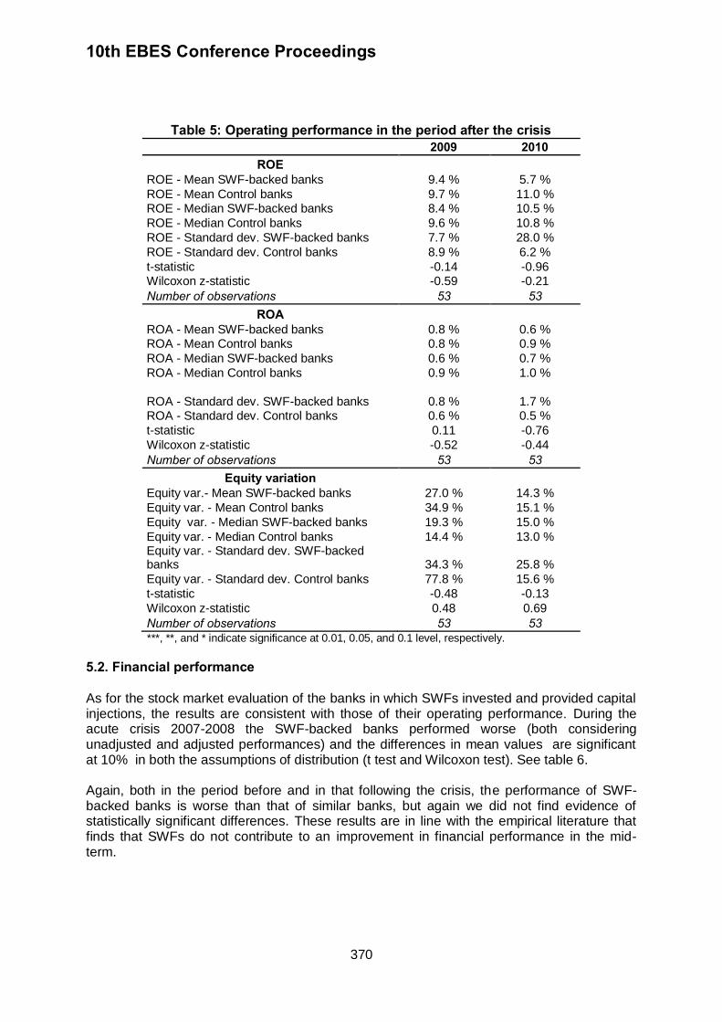
10th EBES Conference Proceedings
370
Table 5: Operating performance in the period after the crisis 2009 2010
ROE ROE - Mean SWF-backed banks 9.4 % 5.7 %
ROE - Mean Control banks 9.7 % 11.0 % ROE - Median SWF-backed banks 8.4 % 10.5 %
ROE - Median Control banks 9.6 % 10.8 %
ROE - Standard dev. SWF-backed banks 7.7 % 28.0 %
ROE - Standard dev. Control banks 8.9 % 6.2 %
t-statistic -0.14 -0.96 Wilcoxon z-statistic -0.59 -0.21
Number of observations 53 53 ROA
ROA - Mean SWF-backed banks 0.8 % 0.6 % ROA - Mean Control banks 0.8 % 0.9 %
ROA - Median SWF-backed banks 0.6 % 0.7 %
ROA - Median Control banks 0.9 % 1.0 %
ROA - Standard dev. SWF-backed banks 0.8 % 1.7 % ROA - Standard dev. Control banks 0.6 % 0.5 %
t-statistic 0.11 -0.76
Wilcoxon z-statistic -0.52 -0.44
Number of observations 53 53 Equity variation
Equity var.- Mean SWF-backed banks 27.0 % 14.3 %
Equity var. - Mean Control banks 34.9 % 15.1 %
Equity var. - Median SWF-backed banks 19.3 % 15.0 %
Equity var. - Median Control banks 14.4 % 13.0 % Equity var. - Standard dev. SWF-backed banks 34.3 % 25.8 %
Equity var. - Standard dev. Control banks 77.8 % 15.6 %
t-statistic -0.48 -0.13
Wilcoxon z-statistic 0.48 0.69
Number of observations 53 53 ***, **, and * indicate significance at 0.01, 0.05, and 0.1 level, respectively.
5.2. Financial performance As for the stock market evaluation of the banks in which SWFs invested and provided capital injections, the results are consistent with those of their operating performance. During the acute crisis 2007-2008 the SWF-backed banks performed worse (both considering unadjusted and adjusted performances) and the differences in mean values are significant at 10% in both the assumptions of distribution (t test and Wilcoxon test). See table 6. Again, both in the period before and in that following the crisis, the performance of SWF-backed banks is worse than that of similar banks, but again we did not find evidence of statistically significant differences. These results are in line with the empirical literature that finds that SWFs do not contribute to an improvement in financial performance in the mid-term.
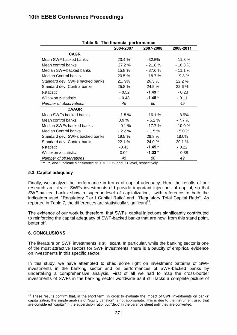
10th EBES Conference Proceedings
371
Table 6: The financial performance 2004-2007 2007-2008 2008-2011
CAGR
Mean SWF-backed banks 23.4 % -32.5% - 11.8 %
Mean control banks 27.2 % - 21.8 % - 10.3 %
Median SWF-backed banks 15.8 % - 37.6 % - 11.1 %
Median Control banks 20.5 % - 18.7 % - 9.3 %
Standard dev. SWFs backed banks 21. 9% 26.3 % 22.2 %
Standard dev. Control banks 25.8 % 24.5 % 22.6 %
t-statistic - 0.52 -1.49 * - 0.23
Wilcoxon z-statistic - 0.48 -1.48 * - 0.11
Number of observations 45 50 49 CAAGR
Mean SWFs backed banks - 1.8 % - 16.1 % - 8.9%
Mean control banks 0.9 % - 5.2 % - 7.7 %
Median SWFs backed banks - 0.1 % - 17.7 % - 10.0 %
Median Control banks - 2.2 % - 1.5 % - 5.0 %
Standard dev. SWFs backed banks 19.5 % 28.8 % 18.0%
Standard dev. Control banks 22.1 % 24.0 % 20.1 %
t-statistic -0.43 -1.45 * - 0.22
Wilcoxon z-statistic 0.04 -1.33 * - 0.38
Number of observations 45 50 49 ***, **, and * indicate significance at 0.01, 0.05, and 0.1 level, respectively.
5.3. Capital adequacy Finally, we analyze the performance in terms of capital adequacy. Here the results of our research are clear: SWFs investments did provide important injections of capital, so that SWF-backed banks show a superior level of capitalization, with reference to both the indicators used: “Regulatory Tier I Capital Ratio” and “Regulatory Total Capital Ratio”. As reported in Table 7, the differences are statistically significant13.
The evidence of our work is, therefore, that SWFs’ capital injections significantly contributed to reinforcing the capital adequacy of SWF-backed banks that are now, from this stand point, better off.
6. CONCLUSIONS The literature on SWF investments is still scant. In particular, while the banking sector is one of the most attractive sectors for SWF investments, there is a paucity of empirical evidence on investments in this specific sector. In this study, we have attempted to shed some light on investment patterns of SWF investments in the banking sector and on performances of SWF-backed banks by undertaking a comprehensive analysis. First of all we had to map the cross-border investments of SWFs in the banking sector worldwide as it still lacks a complete picture of
13
These results confirm that, in the short term, in order to evaluate the impact of SWF investments on banks’ capitalization, the simple analysis of “equity variation” is not appropriate. This is due to the instrument used that are considered “capital” in the supervision ratio, but “debt” in the balance sheet until they are converted.
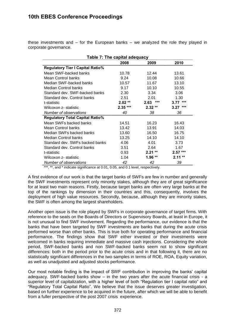
10th EBES Conference Proceedings
372
these investments and – for the European banks – we analyzed the role they played in corporate governance.
Table 7: The capital adequacy
2008 2009 2010 Regulatory Tier I Capital Ratio% Mean SWF-backed banks 10.78 12.44 13.61
Mean Control banks 9.24 10.08 10.66
Median SWF-backed banks 10.57 11.67 13.10
Median Control banks 9.17 10.10 10.55
Standard dev. SWF-backed banks 2.30 3.34 3.06
Standard dev. Control banks 2.51 2.01 1.30
t-statistic 2.02 ** 2.63 *** 3.77 *** Wilcoxon z- statistic 2.35 *** 2.32 ** 3.27 *** Number of observations 40 38 36 Regulatory Total Capital Ratio% Mean SWFs backed banks 14.51 16.23 16.43
Mean Control banks 13.42 13.91 14.03
Median SWFs backed banks 13.60 16.50 16.75
Median Control banks 13.25 14.10 14.10
Standard dev. SWFs backed banks 4.06 4.01 3.73
Standard dev. Control banks 3.51 2.64 1.67
t-statistic 0.93 2.21 ** 2.57 *** Wilcoxon z- statistic 1.04 1.96 ** 2.11 ** Number of observations 42 42 39
***, **, and * indicate significance at 0.01, 0.05, and 0.1 level, respectively.
A first evidence of our work is that the target banks of SWFs are few in number and generally the SWF investments represent only minority stakes, although they are of great significance for at least two main reasons. Firstly, because target banks are often very large banks at the top of the rankings by dimension in their countries and this, consequently, involves the deployment of high value resources. Secondly, because, although they are minority stakes, the SWF is often among the largest shareholders. Another open issue is the role played by SWFs in corporate governance of target firms. With reference to the seats on the Boards of Directors or Supervisory Boards, at least in Europe, it is not unusual to find SWF involvement. Regarding the performance, our evidence is that the banks that have been targeted by SWF investments are banks that during the acute crisis performed worse than other banks. This is true both for operating performance and financial performance. The findings show that SWF either invested or their investments were welcomed in banks requiring immediate and massive cash injections. Considering the whole period, SWF-backed banks and non SWF-backed banks seem not to show significant differences: both in the period prior to the acute crisis and in that following it, there are no statistically significant differences in the two samples in terms of ROE, ROA, Equity variation, as well as unadjusted and adjusted stocks performance. Our most notable finding is the impact of SWF contribution in improving the banks’ capital adequacy. SWF-backed banks show – in the two years after the acute financial crisis - a superior level of capitalization, with a higher level of both “Regulation tier I capital ratio” and “Regulatory Total Capital Ratio”. We believe that the issue deserves greater investigation, based on further experience to be acquired in the future, after which we will be able to benefit from a fuller perspective of the post 2007 crisis experience.
10th EBES Conference Proceedings
373
REFERENCES Avendano, R. and Santiso, J., 2009. Are sovereign wealth funds’ investments politically biased? A comparison with mutual funds. OECD Development Centre Working Paper, 283. Beck, R. and Fidora, M., 2008. The impact of sovereign wealth funds on global financial markets. European Central Bank Occasional Paper, 91.
Bernstein, S., Lerner, J., and Schoar, A., 2009. The investment strategies of sovereign wealth funds. Harvard Business School Working Paper, 09-112.
Bortolotti, B., Fotak, V., Megginson, W., and Miracky W., 2008. Sovereign wealth fund investment patterns and performances. Fondazione Enrico Mattei Nota di lavoro, 22-2009.
Bortolotti B., Fotak V., Megginson W., and Miracky W., 2010. The financial impact of sovereign wealth fund investments in listed companies. Working Paper University of Oklahoma, Monitor Group. Chhaochharia, V. and Laeven, L., 2008a The investment allocation of sovereign wealth funds. [online] Available at: <http://ssrn.com/abstract=1262383> [Accessed 20 May 2013]. Chhaochharia V. and Laeven, L., 2008b. Sovereign wealth funds: Their investment strategies and performance. CEPR Discussion Paper, DP6959.
Clark, G.L. and Monk, A.H.B., 2009. The Oxford survey of sovereign wealth funds' asset managers (July 1st). [online] Available at: <http://ssrn.com/abstract=1432078> [Accessed 20 May 2013].
Dewenter, K., Han, X., and Malatesta P., 2010. Firm values and sovereign wealth fund investments. Journal of Financial Economics, 98(2), pp.256–278.
Drezner, D.W., 2010. BRIC by BRIC: The emergent regime for sovereign wealth funds. In: A.S. Alexandroff and A.F. Cooper, eds. Rising states, rising institutions: Challenges for global governance. Virginia: R.R. Donnelly, pp.218-239.
Fernandes, N., 2009. Sovereign wealth funds: Investment choices and implications around the world. IMD International Working Paper. 2009-01.
IMF, 2008. Sovereign wealth funds - A work agenda. [online] Available at: <http://www.imf.org/external/np/pp/eng/2008/022908.pdf> [Accessed 20 May 2013]. Kern, S., 2008. SWFs and foreign investment policies – An update. Deutsche Bank Research Current Issues, October.
Knill, A., Lee, B., and Mauck N., 2009. ‘Sleeping with the enemy' or 'An ounce of prevention': Sovereign wealth fund investments and market destabilization. [online] Available at: <http://ssrn.com/abstract=1353131> [Accessed 20 May 2013]. Knill, A., Lee, B., and Mauck, N., 2012. Sovereign wealth fund investment and the return-to-risk performance of target firms. Journal of Financial Intermediation, 27(2), pp.315-340.
10th EBES Conference Proceedings
374
Kotter, J. and Lel, U., 2008. Friends or foes? The stock price impact of sovereign wealth fund investments and the price of keeping secrets. International Finance Discussion Papers,
2008-940. Kotter, J. and Lel, U., 2011. Friends or foes? Target selection decisions of sovereign wealth funds and their consequences. Journal of Financial Economics, 101 (2), pp.360–381.
OECD, 2009. Sovereign wealth funds and recipient country policies. [online] Available at: <http://www.oecd.org/dataoecd/34/9/40408735.pdf> [Accessed 20 May 2013]. Raymond, H., 2009. The effect of sovereign wealth funds’ investments on stock markets. EconomiX Working Papers, 2009-38.
Raymond, H., 2010. Sovereign wealth funds as domestic investors of last resort during crises. International Economics, 123(3), pp.121-159.
Razanov, A., 2005. Who holds the wealth of nations? Central Banking Journal, 15(4), pp.52-
57. Sun, T. and Hesse, H., 2009. Sovereign wealth funds and financial stability - An event study analysis. IMF Working Paper, 09/239. Truman, E.M., 2008. A blueprint for sovereign wealth fund best practices. Policy Brief, Peterson Institute for International Economics, Pb08-3.
10th EBES Conference Proceedings 23 - 25 May, 2013. NIPPON HOTEL, ISTANBUL, TURKEY ISBN: 978-605-64002-1-6. WEBSITE: www.ebesweb.org
375
THE KNOWLEDGE ECONOMY IN THE WESTERN BALKAN COUNTRIES AND TURKEY
SHENAJ HADZIMUSTAFA
Faculty of Business and Economics South East European University
Republic of Macedonia [email protected]
GADAF REXHEPI
Faculty of Business and Economics South East European University
Republic of Macedonia [email protected]
SADUDIN IBRAIMI
Faculty of Business and Economics South East European University
Republic of Macedonia [email protected]
NEXHBI VESELI
Faculty of Business and Economics South East European University
Republic of Macedonia [email protected]
Abstract: Knowledge has become the major driving force of economic and social development all around the world and it impacts all countries and regions, public institutions, the corporate world, and the lives and prospects of individuals. The generation and conversion of knowledge into economic and social benefits requires good innovation systems, including highly qualified personnel and efficient technology transfer (TT) and venture capital. Higher levels of knowledge in a society tend to lead to higher levels of economic growth – and consequently to higher levels of economic development. This paper assesses the role of the knowledge economy, in the terms of achieving long-term economic growth in the selected countries. Based on an analysis of data on an array of indicators, each of which represents an aspect of the knowledge economy, the paper shows the stage in which each of the selected countries is concerning the knowledge economy. Western Balkan countries and Turkey should put themselves on the knowledge economy road and create a more competitive economy with highly skilled and educated workforce that with the use of ICT can create more innovative products that will decrease the transaction costs and create higher economic values and improvement of the economic productivity. Keywords: Knowledge Economy, Economic Growth, Economic Development, Knowledge, Sustainability

10th EBES Conference Proceedings
376
1. INTRODUCTION Knowledge has always been an essential force in economic development. But in today’s increasingly knowledge-based world, more and more countries are embracing knowledge and innovation-related policies to spur growth and competitiveness. At the same time, many developing countries are struggling to find ways to produce relevant knowledge and transform it into wealth, as well as to adapt and disseminate existing knowledge for their development. In an agricultural economy land is the key resource. In industrial economy natural resources, such as coal and iron ore and labour are the main resources. Knowledge economy is one in which knowledge is the key resource. It is not a new idea that knowledge plays an important role in the economy, nor is it a new fact. All economies, even the least-developed ones, are based on knowledge about how, for example, to farm, to mine and to build; and this use of knowledge has been increasing since the Industrial Revolution. But the degree of incorporation of knowledge and information into economic activity is now so great that it is inducing quite profound structural and qualitative changes in the operation of the economy and transforming the basis of competitive advantage. The rising knowledge intensity of the world economy and peoples increasing ability to distribute that knowledge has increased its value to all participants in the economic system. The implications of this are profound, not only for the strategies of firms and for the policies of government but also for the institutions and systems used to regulate economic behaviour. Ten years ago, Europe’s leaders set an ambitious goal of becoming “the most competitive and dynamic knowledge-based economy in the world” by 2010 through a programme of policy initiatives known as the Lisbon Strategy. The objective of the Lisbon Strategy was to improve Europe’s productivity and competitiveness through various policy initiatives, building on a number of earlier goals. These included the creation of an information society for all, establishing a European area of research and development, developing a business-friendly start-up environment, completing the single market, establishing efficient and integrated financial markets, building a knowledge society, ensuring more and better jobs for Europe, modernizing social protection, promoting social inclusion and enhancing sustainable development. The recent economic crisis has underscored the importance of a
competitiveness-supporting economic environment to better enable national economies to absorb shocks and ensure solid economic performance going into the future (Schwab 2010). Given that the Lisbon Strategy is set to expire this year, the EU has been preparing a new 10-year growth strategy to replace it in an effort to improve the process this time around. This has been termed “Europe 2020”, which seeks to enhance the delivery of growth and jobs for the next decade. At the heart of the agenda is a goal of “smart, sustainable, inclusive growth brought about through greater coordination of national and European policy.” To reinforce the ability to meet these targets, the strategy also identifies seven flagship initiatives the EU should take to boost growth and employment (Schwab 2010): 1. “Innovation union” to improve framework conditions and access to finance for research
and innovation to ensure that innovative ideas can be turned into products and services that create growth and jobs
2. “Youth on the move” to enhance the performance of education systems and facilitate the entry of young people into the labour market
3. “A digital agenda for Europe” to speed up the roll-out of high-speed Internet and reap the benefits of a digital single market for households and firms

10th EBES Conference Proceedings
377
4. “Resource-efficient Europe” to help decouple economic growth from the use of resources, supports the shift towards a low-carbon economy, increase the use of renewable energy sources, modernize the transport sector and promote energy efficiency
5. “An industrial policy for the globalization era” to improve the business environment, notably for SMEs, and to support the development of a strong and sustainable industrial base able to compete globally
6. “An agenda for new skills and jobs” to modernize labour markets and empower people by developing their skills throughout the lifecycle with a view to increase labour participation and better match labour supply and demand, including through labour mobility
7. “European platform against poverty” to ensure social and territorial cohesion such that the benefits of growth and jobs are widely shared and people experiencing poverty and social exclusion are enabled to live in dignity and take an active part in society. The core of meeting the Europe 2020 strategy is the knowledge economy which should lead toward sustainable growth and development of the countries. 2. SUSTAINABLE ECONOMIC GROWTH AND DEVELOPMENT Economic growth is the result of the accumulation of factors and increases in productivity. The significant differences in rates of growth among world countries are due much more to differences in productivity behaviour than to factor accumulation. But both growth sources tend to be affected by common variables and, in particular, by society’s capacity to assimilate and generate knowledge and technologies and apply them to productive activities and by the opportunities that enterprises and individuals have to gain ownership of the results of their own efforts. Growth is achieved by increasing the productivity of existing investments or by making larger investments, or a combination of both. It is therefore important to improve the overall climate in which these investments are made and developed. (Inter - American Development Bank 2003). Achieving sustainable economic growth is necessary to reduce poverty. Growth provides the flow of resources needed for employment and income generation, and for the financing of programs geared towards poverty alleviation. At the same time, a number of studies have shown that persistent inequality limits a country’s growth potential. Accordingly, addressing the levels of inequality in human capital and access to productive assets for the poor will help generate more opportunities for their inclusion in economic activities and will contribute to growth (Inter - American Development Bank 2003). Therefore, advances in poverty reduction and the promotion of equity are a fundamental development goal. Economic and social development strategies must therefore include growth policies and specific actions for the poorest population, excluded groups, and low-income geographic areas. Clearly, the two objectives of poverty reduction and sustainable economic growth are compatible and renewed efforts are needed to promote growth and to ensure that the benefits of that growth accrue to the poor. While the overarching goals are closely interrelated, complementarity is not automatic, as it depends on the selection and orientation of policy instruments and on the attention given to their sustainability (Inter - American Development Bank 2003). Economic growth comes in two forms: an economy can either grow “extensively” by using more resources (such as physical, human, or natural capital) or “intensively” by using the
same amount of resources more efficiently (productively). When economic growth is achieved by using more labour, it does not result in per capita income growth. But when economic growth is achieved through more productive use of all resources, including labour, it results in higher per capita income and improvement in people’s average standard of living (Soubbotina 2004).
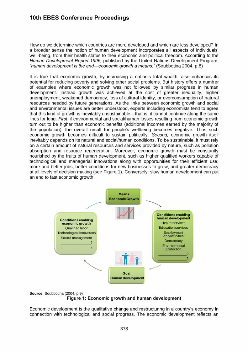
10th EBES Conference Proceedings
378
How do we determine which countries are more developed and which are less developed? In a broader sense the notion of human development incorporates all aspects of individuals’ well-being, from their health status to their economic and political freedom. According to the Human Development Report 1996, published by the United Nations Development Program, “human development is the end—economic growth a means.” (Soubbotina 2004, p.8)
It is true that economic growth, by increasing a nation’s total wealth, also enhances its potential for reducing poverty and solving other social problems. But history offers a number of examples where economic growth was not followed by similar progress in human development. Instead growth was achieved at the cost of greater inequality, higher unemployment, weakened democracy, loss of cultural identity, or overconsumption of natural resources needed by future generations. As the links between economic growth and social and environmental issues are better understood, experts including economists tend to agree that this kind of growth is inevitably unsustainable—that is, it cannot continue along the same lines for long. First, if environmental and social/human losses resulting from economic growth
turn out to be higher than economic benefits (additional incomes earned by the majority of the population), the overall result for people’s wellbeing becomes negative. Thus such economic growth becomes difficult to sustain politically. Second, economic growth itself inevitably depends on its natural and social/human conditions. To be sustainable, it must rely on a certain amount of natural resources and services provided by nature, such as pollution absorption and resource regeneration. Moreover, economic growth must be constantly nourished by the fruits of human development, such as higher qualified workers capable of technological and managerial innovations along with opportunities for their efficient use: more and better jobs, better conditions for new businesses to grow, and greater democracy at all levels of decision making (see Figure 1). Conversely, slow human development can put an end to fast economic growth.
MeansEconomic Growth
Conditions enabling human development
Health services
Education services
Employment opportunities
Democracy
Environmental protection
_______________?
_______________?
Goal:Human development
Conditions enabling economic growth
Qualified labor
Technological innovations
Sound management
________________?
________________?
Source: Soubbotina (2004, p.9)
Figure 1: Economic growth and human development Economic development is the qualitative change and restructuring in a country’s economy in connection with technological and social progress. The economic development reflects an
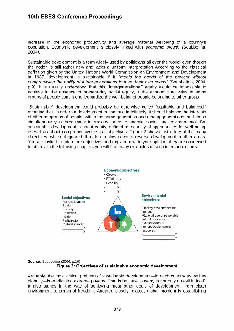
10th EBES Conference Proceedings
379
increase in the economic productivity and average material wellbeing of a country’s population. Economic development is closely linked with economic growth (Soubbotina, 2004). Sustainable development is a term widely used by politicians all over the world, even though the notion is still rather new and lacks a uniform interpretation According to the classical definition given by the United Nations World Commission on Environment and Development in 1987, development is sustainable if it “meets the needs of the present without compromising the ability of future generations to meet their own needs” (Soubbotina, 2004,
p.9). It is usually understood that this “intergenerational” equity would be impossible to achieve in the absence of present-day social equity, if the economic activities of some groups of people continue to jeopardize the well-being of people belonging to other group. “Sustainable” development could probably be otherwise called “equitable and balanced,” meaning that, in order for development to continue indefinitely, it should balance the interests of different groups of people, within the same generation and among generations, and do so simultaneously in three major interrelated areas–economic, social, and environmental. So, sustainable development is about equity, defined as equality of opportunities for well-being, as well as about comprehensiveness of objectives. Figure 2 shows just a few of the many objectives, which, if ignored, threaten to slow down or reverse development in other areas. You are invited to add more objectives and explain how, in your opinion, they are connected to others. In the following chapters you will find many examples of such interconnections.
Economic objectives:• Growth
• Efficiency
• Stability
•______?
•______?Environmental objectives:
•Healthy environment for
humans
•Rational use of renewable
natural resources
•Conservation of
nonrenewable natural
resources
•___________________?
•___________________?
Social objectives•Full employment
•Equity
•Security
•Education
•Health
•Participation
•Cultural identity
•____________?
•____________?
Source: Soubbotina (2004, p.10)
Figure 2: Objectives of sustainable economic development Arguably, the most critical problem of sustainable development—in each country as well as globally—is eradicating extreme poverty. That is because poverty is not only an evil in itself. It also stands in the way of achieving most other goals of development, from clean environment to personal freedom. Another, closely related, global problem is establishing
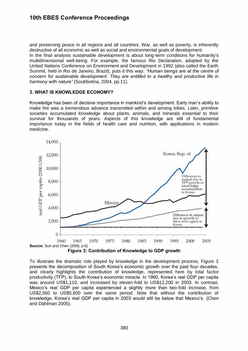
10th EBES Conference Proceedings
380
and preserving peace in all regions and all countries. War, as well as poverty, is inherently destructive of all economic as well as social and environmental goals of development. In the final analysis sustainable development is about long-term conditions for humanity’s multidimensional well-being. For example, the famous Rio Declaration, adopted by the United Nations Conference on Environment and Development in 1992 (also called the Earth Summit, held in Rio de Janeiro, Brazil), puts it this way: “Human beings are at the centre of concern for sustainable development. They are entitled to a healthy and productive life in harmony with nature” (Soubbotina, 2004, pp.11). 3. WHAT IS KNOWLEDGE ECONOMY? Knowledge has been of decisive importance in mankind’s development. Early man’s ability to make fire was a tremendous advance transmitted within and among tribes. Later, primitive societies accumulated knowledge about plants, animals, and minerals essential to their survival for thousands of years. Aspects of this knowledge are still of fundamental importance today in the fields of health care and nutrition, with applications in modern medicine.
Source: Suh and Chen (2006, p.6)
Figure 3: Contribution of Knowledge to GDP growth To illustrate the dramatic role played by knowledge in the development process, Figure 3 presents the decomposition of South Korea’s economic growth over the past four decades, and clearly highlights the contribution of knowledge, represented here by total factor productivity (TFP), to South Korea’s economic miracle. In 1960, Korea’s real GDP per capita was around US$1,110, and increased by eleven-fold to US$12,200 in 2003. In contrast, Mexico’s real GDP per capita experienced a slightly more than two-fold increase, from US$2,560 to US$5,800 over the same period. Note that without the contribution of knowledge, Korea’s real GDP per capita in 2003 would still be below that Mexico’s. (Chen and Dahlman 2005).
10th EBES Conference Proceedings
381
Knowledge is special because it is difficult to obtain, whether through creation or purchase. Unlike information, knowledge involves combinations of facts that interact in intangible ways. Because it is difficult to obtain, it constitutes an entry barrier to growth—and this entry barrier, in turn, helps generate the rent earned from knowledge. There are several types of knowledge rent: technological (control of scarce process or product capabilities), human resources (availability of unique or advanced human skills and know-how), organizational (control of unique or advanced management practices), and marketing and design (both increasingly important in recent years, with a direct correlation to consumer know-how) (WBI 2007). Knowledge influences competitiveness, economic growth, and development as long as it finds concrete applications—in other words, as long as it is at work. The need to assess the importance of technological progress for sustainable growth, including related investments such as education, created the impetus for new growth theories that have tried to endogenize (or “include”) technological progress in their models. These new theories and related econometric models help explain why countries’ economic trajectories tend to diverge, and therefore help justify government action and investment in public goods such as education and infrastructure, which facilitate the use of knowledge and innovation. With sustained use and creation of knowledge at the center of the economic development process, an economy essentially becomes a Knowledge Economy. A Knowledge Economy (KE) is one that utilizes knowledge as the key engine of economic growth. It is an economy
where knowledge is acquired, created, disseminated and used effectively to enhance economic development Over the past quarter century, the rate of knowledge creation and dissemination has increased significantly. One reason is due to the rapid advances in information and communications technologies (ICTs) that have significantly decreased the costs of computing power and electronic networking. With the increased affordability, the usage of computing power and electronic networking has surged, along with the efficient dissemination of existing knowledge. Modern ICTs also enable researchers in different locations to work together, which consequently enhance the productivity of researchers, resulting in rapid advances in research and development and the generation of new knowledge and technologies. One indicator of the creation of new knowledge and technologies is the number of patents granted by the United States Patent and Trademark Office (USPTO)1 each year (Chen and Dahlman 2005). Patent documents include utility patents, design patents, plant patents, reissue patents, defensive publications and statutory invention registration. The number of patents are important indicator of the innovation presence in the economy, that is one of the crucial pillars in the knowledge economy that enables positive economic growth. The increased speed in the creation and dissemination of knowledge has led to the rapid spread of modern and efficient production techniques, plus the increased probability of leapfrogging, which has consequently resulted in the world economy becoming much more competitive. In addition to the higher level of competition, the nature of competition has been changing. It has evolved from one that was just based on cost, to one where speed and innovation are also essential. Commodity production is usually allocated to lowest cost producers, but intense competition resulting from globalization tends to drive profits from commodity production to nearly zero. As such, it has become crucial to derive additional
1 The United States Patent and Trademark Office (PTO or USPTO) is an agency in the United States Department
of Commerce that issues patents to inventors and businesses for their inventions, and trademark registration for product and intellectual property identification.
10th EBES Conference Proceedings
382
value added from various means of product differentiation via innovative designs, effective marketing, efficient distribution, reputable brand names, etc. Thus, to prosper it is critical to be able to contribute productively to global value chains and to generate own new value chains, and the key part of which is not necessarily production, but innovation and high-value services. In light of the above, sustained economic growth in the era of this new world economy depends on developing successful strategies that involve the sustained use and creation of knowledge at the core of the development process. At lower levels of development, which typically implies lower levels of science and technology capability, knowledge strategies typically involve the tapping of existing global knowledge and adoption of such foreign technologies to local conditions in order to enhance domestic productivity. At higher levels of development, which typically implies higher levels of science and technology capability, knowledge strategies also hinges critically on domestic innovative effort and underlie the move to produce products and services that higher value-added in order to be consistent with the high wages that are characteristic of these economies. The emergence of the knowledge economy can be characterized in terms of the increasing role of knowledge as a factor of production and its impact on skills, learning, organization and innovation (Houghton and Sheehan 2000). There is an enormous increase in the codification of knowledge, which together with networks and the digitalisation of information, is leading to its increasing co modification. Increasing codification of knowledge is leading to a shift in the balance of the stock of knowledge – leading to a relative shortage of tacit knowledge. Codification is promoting a shift in the organisation and structure of production. Information and communication technologies increasingly favour the diffusion of information over re-invention, reducing the investment required for a given quantum of knowledge. The increasing rate of accumulation of knowledge stocks is positive for economic growth (raising the speed limit to growth). Knowledge is not necessarily exhausted in consumption. Codification is producing a convergence, bridging different areas of competence, reducing knowledge dispersion, and increasing the speed of turnover of the stock of knowledge. The innovation system and its ‘knowledge distribution power’ are critically important. The increased rate of codification and collection of information are leading to a shift in focus towards tacit (‘handling’) skills. Learning is increasingly central for both people and organizations. Learning involves both education and learning-by-doing, learning-by-using and learning-by-interacting. Learning organisations are increasingly networked organizations. Initiative, creativity, problem solving and openness to change are increasingly important skills. The transition to a knowledge-based system may make market failure systemic. A knowledge-based economy is so fundamentally different from the resource based system of the last century that conventional economic understanding must be re-examined.
4. THE KNOWLEDGE ECONOMY FRAMEWORK It has been found that the successful transition to the Knowledge Economy typically involves elements such as long-term investments in education, developing innovation capability, modernizing the information infrastructure, and having an economic environment that is conducive to market transactions. These elements have been termed by the World Bank as the pillars of the Knowledge Economy and together they constitute the Knowledge Economy framework. More specifically, the four pillars of the Knowledge Economy (KE) framework are (Chen and Dahlman 2005):
• An economic incentive and institutional regime that provides good economic policies and institutions that permit efficient mobilization and allocation of resources and
10th EBES Conference Proceedings
383
stimulate creativity and incentives for the efficient creation, dissemination, and use of existing knowledge.
• Educated and skilled workers who can continuously upgrade and adapt their skills to
efficiently create and use knowledge. • An effective innovation system of firms, research centers, universities, consultants, and
other organizations that can keep up with the knowledge revolution and tap into the growing stock of global knowledge and assimilate and adapt it to local needs.
• A modern and adequate information infrastructure that can facilitate the effective communication, dissemination, and processing of information and knowledge.
The Knowledge Economy framework thus asserts that investments in the four knowledge economy pillars are necessary for sustained creation, adoption, adaptation and use of knowledge in domestic economic production, which will consequently result in higher value added goods and services. This would tend to increase the probability of economic success, and hence economic development, in the current highly competitive and globalized world economy. The labor force should be composed of educated and skilled workers who are able to continuously upgrade and adapt their skills to create and use knowledge efficiently. Education and training systems encompass primary and secondary education, vocational training, higher education, and lifelong learning. The weight placed on the different segments will differ somewhat depending on a country’s level of development. For example, basic education will receive more attention at low levels of development, as basic literacy and numeracy are necessary foundations on which more advanced skills are built. Similarly, lifelong learning has increasing importance in the current context of the knowledge revolution, which requires constant adaptation of knowledge and know-how. It also grows in importance as the population ages. Globalization, meanwhile, is bridging the distance between basic skill needs and advanced skills, forcing countries to cover a wide educational band even at low levels of development to catch up with advanced economies and then remain competitive. A modern and adequate information infrastructure will facilitate the effective communication, dissemination, and
processing of information and knowledge. Information and communication technologies (ICTs)—including telephone, television, and radio networks—are the essential infrastructure of the global, information-based economies of our time, as railways, roads, and utilities were in the industrial era. They can considerably reduce transaction costs by providing ready access to information. ICT-related policies cover telecommunications regulation as well as the investments needed to build and exploit ICTs throughout the economy and society through various “e-applications”—e-government, e-business, e-learning, etc. Low-income countries should focus first on the basic ICT infrastructure before promoting advanced technologies and applications. An effective innovation system is composed of firms, research centers, universities,
consultants, and other organizations that keep up with new knowledge and technology, tap into the growing stock of global knowledge, and assimilate and adapt it to local needs. Public support for innovation, science, and technology covers a wide range of infrastructure and institutional functions, from the diffusion of basic technologies to advanced research activities. The former should receive a great deal of attention in developing countries. For most developing countries much of the knowledge and technology that nurtures innovation will originate from foreign sources, entering the country throgh foreign direct investment (FDI), imports of equipment and other goods, and licensing agreements. Foreign sources are important when the economy is less developed, though imports must not be allowed to
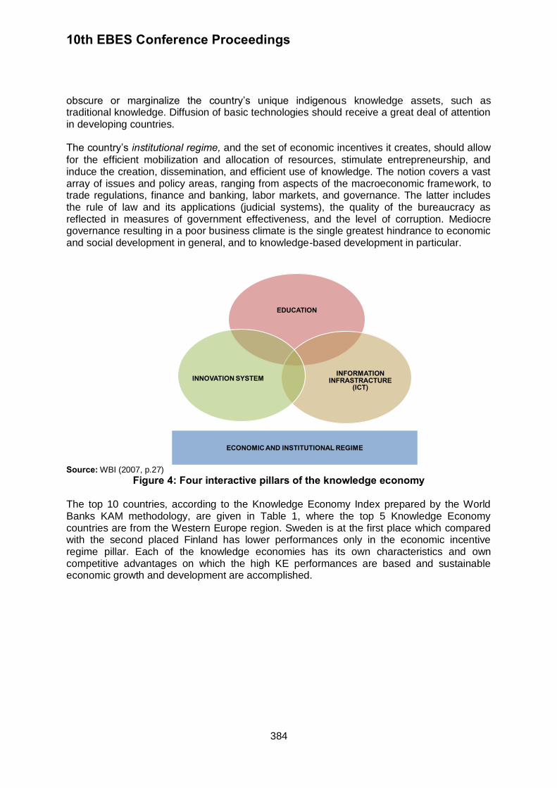
10th EBES Conference Proceedings
384
obscure or marginalize the country’s unique indigenous knowledge assets, such as traditional knowledge. Diffusion of basic technologies should receive a great deal of attention in developing countries. The country’s institutional regime, and the set of economic incentives it creates, should allow
for the efficient mobilization and allocation of resources, stimulate entrepreneurship, and induce the creation, dissemination, and efficient use of knowledge. The notion covers a vast array of issues and policy areas, ranging from aspects of the macroeconomic framework, to trade regulations, finance and banking, labor markets, and governance. The latter includes the rule of law and its applications (judicial systems), the quality of the bureaucracy as reflected in measures of government effectiveness, and the level of corruption. Mediocre governance resulting in a poor business climate is the single greatest hindrance to economic and social development in general, and to knowledge-based development in particular.
EDUCATION
INFORMATION INFRASTRACTURE
(ICT)INNOVATION SYSTEM
ECONOMIC AND INSTITUTIONAL REGIME
Source: WBI (2007, p.27)
Figure 4: Four interactive pillars of the knowledge economy The top 10 countries, according to the Knowledge Economy Index prepared by the World Banks KAM methodology, are given in Table 1, where the top 5 Knowledge Economy countries are from the Western Europe region. Sweden is at the first place which compared with the second placed Finland has lower performances only in the economic incentive regime pillar. Each of the knowledge economies has its own characteristics and own competitive advantages on which the high KE performances are based and sustainable economic growth and development are accomplished.
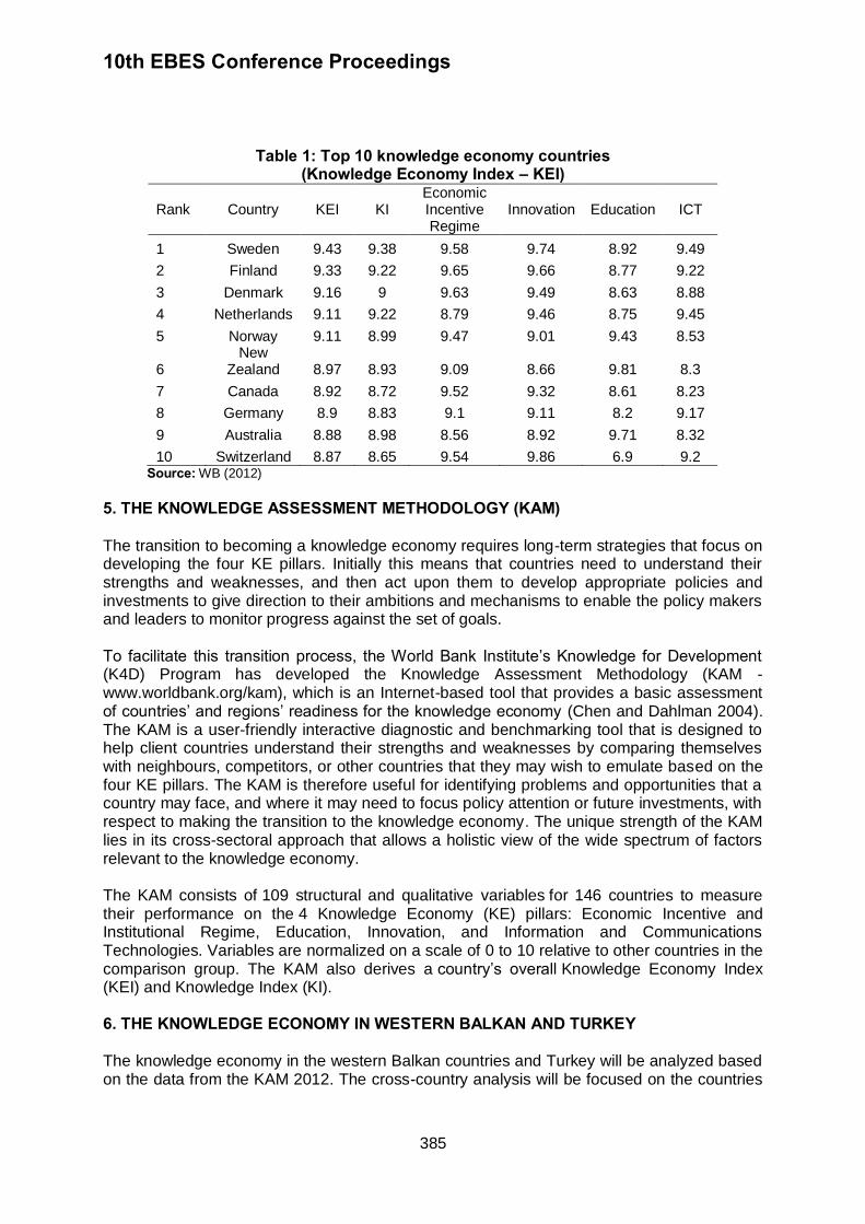
10th EBES Conference Proceedings
385
Table 1: Top 10 knowledge economy countries (Knowledge Economy Index – KEI)
Rank Country KEI KI Economic Incentive Regime
Innovation Education ICT
1 Sweden 9.43 9.38 9.58 9.74 8.92 9.49
2 Finland 9.33 9.22 9.65 9.66 8.77 9.22
3 Denmark 9.16 9 9.63 9.49 8.63 8.88
4 Netherlands 9.11 9.22 8.79 9.46 8.75 9.45
5 Norway 9.11 8.99 9.47 9.01 9.43 8.53
6 New
Zealand 8.97 8.93 9.09 8.66 9.81 8.3
7 Canada 8.92 8.72 9.52 9.32 8.61 8.23
8 Germany 8.9 8.83 9.1 9.11 8.2 9.17
9 Australia 8.88 8.98 8.56 8.92 9.71 8.32
10 Switzerland 8.87 8.65 9.54 9.86 6.9 9.2 Source: WB (2012)
5. THE KNOWLEDGE ASSESSMENT METHODOLOGY (KAM) The transition to becoming a knowledge economy requires long-term strategies that focus on developing the four KE pillars. Initially this means that countries need to understand their strengths and weaknesses, and then act upon them to develop appropriate policies and investments to give direction to their ambitions and mechanisms to enable the policy makers and leaders to monitor progress against the set of goals. To facilitate this transition process, the World Bank Institute’s Knowledge for Development (K4D) Program has developed the Knowledge Assessment Methodology (KAM - www.worldbank.org/kam), which is an Internet-based tool that provides a basic assessment of countries’ and regions’ readiness for the knowledge economy (Chen and Dahlman 2004). The KAM is a user-friendly interactive diagnostic and benchmarking tool that is designed to help client countries understand their strengths and weaknesses by comparing themselves with neighbours, competitors, or other countries that they may wish to emulate based on the four KE pillars. The KAM is therefore useful for identifying problems and opportunities that a country may face, and where it may need to focus policy attention or future investments, with respect to making the transition to the knowledge economy. The unique strength of the KAM lies in its cross-sectoral approach that allows a holistic view of the wide spectrum of factors relevant to the knowledge economy. The KAM consists of 109 structural and qualitative variables for 146 countries to measure their performance on the 4 Knowledge Economy (KE) pillars: Economic Incentive and Institutional Regime, Education, Innovation, and Information and Communications Technologies. Variables are normalized on a scale of 0 to 10 relative to other countries in the comparison group. The KAM also derives a country’s overall Knowledge Economy Index (KEI) and Knowledge Index (KI). 6. THE KNOWLEDGE ECONOMY IN WESTERN BALKAN AND TURKEY The knowledge economy in the western Balkan countries and Turkey will be analyzed based on the data from the KAM 2012. The cross-country analysis will be focused on the countries
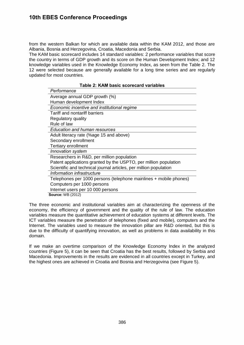
10th EBES Conference Proceedings
386
from the western Balkan for which are available data within the KAM 2012, and those are Albania, Bosnia and Herzegovina, Croatia, Macedonia and Serbia. The KAM basic scorecard includes 14 standard variables: 2 performance variables that score the country in terms of GDP growth and its score on the Human Development Index; and 12 knowledge variables used in the Knowledge Economy Index, as seen from the Table 2. The 12 were selected because are generally available for a long time series and are regularly updated for most countries.
Table 2: KAM basic scorecard variables Performance Average annual GDP growth (%)
Human development Index
Economic incentive and institutional regime Tariff and nontariff barriers
Regulatory quality
Rule of law
Education and human resources Adult literacy rate (%age 15 and above)
Secondary enrollment
Tertiary enrollment
Innovation system Researchers in R&D, per million population Patent applications granted by the USPTO, per million population
Scientific and technical journal articles, per million population
Information infrastructure Telephones per 1000 persons (telephone mainlines + mobile phones)
Computers per 1000 persons
Internet users per 10 000 persons Source: WB (2012)
The three economic and institutional variables aim at characterizing the openness of the economy, the efficiency of government and the quality of the rule of law. The education variables measure the quantitative achievement of education systems at different levels. The ICT variables measure the penetration of telephones (fixed and mobile), computers and the Internet. The variables used to measure the innovation pillar are R&D oriented, but this is due to the difficulty of quantifying innovation, as well as problems in data availability in this domain. If we make an overtime comparison of the Knowledge Economy Index in the analyzed countries (Figure 5), it can be seen that Croatia has the best results, followed by Serbia and Macedonia. Improvements in the results are evidenced in all countries except in Turkey, and the highest ones are achieved in Croatia and Bosnia and Herzegovina (see Figure 5).
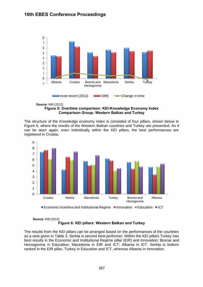
10th EBES Conference Proceedings
387
Source: WB (2012)
Figure 5: Overtime comparison: KEI-Knowledge Economy Index Comparison Group: Western Balkan and Turkey
The structure of the Knowledge economy index is consisted of four pillars, shown below in Figure 6, where the results of the Western Balkan countries and Turkey are presented. As it can be seen again, even individually within the KEI pillars, the best performances are registered in Croatia.
Source: WB (2012)
Figure 6: KEI pillars: Western Balkan and Turkey The results from the KEI pillars can be arranged based on the performances of the countries as a rank given in Table 3. Serbia is second best performer. Within the KEI pillars Turkey has best results in the Economic and Institutional Regime pillar (EIR) and Innovation; Bosnia and Herzegovina in Education; Macedonia in EIR and ICT; Albania in ICT. Serbia is bottom ranked in the EIR pillar, Turkey in Education and ICT, whereas Albania in Innovation.
-1
0
1
2
3
4
5
6
7
8
Albania Croatia Bosnia and Herzegovina
Macedonia Serbia Turkey
most recent (2012) 1995 Change in time
0
1
2
3
4
5
6
7
8
9
Croatia Serbia Macedonia Turkey Bosnia and Herzegovina
Albania
Economic Incentive and Institutional Regime Innovation Education ICT

10th EBES Conference Proceedings
388
Table 3: KEI pillars country ranking
Rank KEI Economic Incentive and Institutional Regime (EIR)
Innovation Education ICT
1 Croatia Croatia Croatia Croatia Croatia
2 Serbia Turkey Serbia Serbia Serbia
3 Macedonia Macedonia Turkey Bosnia and Herzegovina Macedonia
4 Turkey Bosnia and Herzegovina Macedonia Macedonia Albania
5 Bosnia and Herzegovina Albania
Bosnia and Herzegovina Albania
Bosnia and Herzegovina
6 Albania Serbia Albania Turkey Turkey Source: WB (2012)
The KEI pillars are based on the results that the countries have achieved in the different variables that consists each KEI pillar, as given in Table 2. If we go through the KEI variable performances of the countries we can see that Croatia has the highest values, with an exception in the variables concerning the average years of schooling, where Albania is the best performer with a result of 7.56 (out of 10), and Gross Tertiary enrolment rate, where Serbia with 6.31, has a little higher result compared to Croatia with 6.24. Bosnia and Herzegovina is a trade opened country that can be seen from the high results in tariff and nontariff barriers and also has good performances in the gross secondary enrolment rate, right after Croatia and Serbia. Macedonia’s good performances in the ICT pillar are based on the good results in the computers per 1000 people and internet user per 1000 people variables, where is right after Croatia and Serbia, respectively. Turkey has very good results in all of the variables concerning the EIR pillar, and has very high performances in the S&E Journal Articles /Mil. People pillar, together with Croatia and Serbia that is giving a base for the good innovation pillar results, as shown in Figure 7 and Table 3. Serbia has high performances in the ICT pillar variables such as Total Telephones per 1000 People and Internet Users per 1000 People (in front of Croatia).
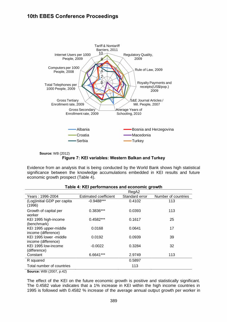
10th EBES Conference Proceedings
389
Source: WB (2012)
Figure 7: KEI variables: Western Balkan and Turkey Evidence from an analysis that is being conducted by the World Bank shows high statistical significance between the knowledge accumulations embedded in KEI results and future economic growth prospect (Table 4).
Table 4: KEI performances and economic growth RegA2
Years : 1996-2004 Estimated coefficient Standard error Number of countries
(Log)initial GDP per capita (1996)
-0.9488*** 0.4102 113
Growth of capital per worker
0.3836***
0.0393 113
KEI 1995 high-income (benchmark)
0.4582*** 0.1617 25
KEI 1995 upper-middle income (difference)
0.0168 0.0641 17
KEI 1995 lower -middle income (difference)
0.0192 0.0939 39
KEI 1995 low-income (difference)
-0.0022 0.3284 32
Constant 6.6641*** 2.9749 113
R squared 0.5897
Total number of countries 113
Source: WBI (2007, p.42)
The effect of the KEI on the future economic growth is positive and statistically significant. The 0.4582 value indicates that a 1% increase in KEI within the high income countries in 1995 is followed with 0.4582 % increase of the average annual output growth per worker in
0
2
4
6
8
10
Tariff & Nontariff Barriers, 2011
Regulatory Quality, 2009
Rule of Law, 2009
Royalty Payments and receipts(US$/pop.)
2009
S&E Journal Articles / Mil. People, 2007
Average Years of Schooling, 2010
Gross Secondary Enrollment rate, 2009
Gross Tertiary Enrollment rate, 2009
Total Telephones per 1000 People, 2009
Computers per 1000 People, 2008
Internet Users per 1000 People, 2009
Albania Bosnia and Herzegovina
Croatia Macedonia
Serbia Turkey

10th EBES Conference Proceedings
390
the 1996-2004 period of time. This value for the upper-middle income countries is 0.0168 and is not statistically significant. It shows that the estimated effect of the KEI on the future economic growth is higher than the one in the high income countries for 0.0168 units that implicate 0.4750 net effects, and so on. Taking into consideration that the knowledge accumulation has a positive impact on the economic growth, countries should practice policies that are based on knowledge that should be used when creating the development strategies. The consistent policies within the countries have vast importance for the achievement of higher performances in the KEI variables and pillars that lead towards higher economic growth results. 7. CONCLUSION With the spread of modern and efficient information and communication technologies, the world economy has become more competitive as well as interdependent. As such, economic survival made it essential to have knowledge creation, dissemination and use play a focal point in long-term developmental strategies. In other words, it is critical for countries make the transition to become a Knowledge Economy. This paper also presents the Knowledge Economy framework thus asserts that information infrastructure, and a conducive economic incentive and institutional regime are necessary for sustained creation, adoption, adaptation and use of knowledge in domestic economic production, which will consequently result in higher value added goods and services. This would tend to increase the probability of economic success, and hence economic development, in the current highly competitive and globalized world economy. Taking into consideration the fact that the knowledge economy is essential for the economic growth and development of the countries and their global competitiveness, the government actions and the policy making processes should support the movement of the countries on the knowledge economy path. The Western Balkan countries and Turkey are on the path toward knowledge economy, although a number of reforms still have to be undertaken. The consistent policies will foster this direction and result with higher rates of economic growth in the countries. REFERENCES Chen, D., 2006. Koreas as a knowledge economy: Overview. Washington D.C.: IBRD/WB.
Chen, D., Dahlman, C., 2004. Knowledge and development: A cross section approach, Washington D.C.: World Bank. Chen, D., Dahlman, C., 2005. The knowledge economy, the KAM methodology and world bank operations. Washington D.C.: The World Bank.
Houghton, J. ans Sheehan, P., 2000. A primer on the knowledge economy, Melbourne: Centre for Strategic Economic Studies, Victoria University. Inter-American Development Bank, 2003. Sustainable economic growth: Strategy document,. Washington D.C. Schwab, K., 2010. The global competitiveness report 2010-2011. Geneva: World Economic Forum

10th EBES Conference Proceedings
391
Soubbotina, T.P., 2004. Beyond economic growth,An introduction to sustainable development. Washington D.C.: The World Bank.
Suh, J., and Chen, D., 2006. Korea as a knowledge economy: Evolutionary process and lessons learned. Washington D.C.: The World Bank.
WB, 2012. Knowledge assesment methodology. [Online] Available at: <http://info.worldbank.org/etools/kam2/KAM_page5.asp> [Accessed 5 May 2013]. WBI, 2007. Building knowledge economies. Washington, DC: IBRD/The World Bank.
10th EBES Conference Proceedings 23 - 25 May, 2013. NIPPON HOTEL, ISTANBUL, TURKEY ISBN: 978-605-64002-1-6. WEBSITE: www.ebesweb.org
392
ITALIAN GOVERNMENT BONDS: AN EMPIRICAL STUDY
GABRIELLA FOSCHINI Department of Economic & Political Sciences & Modern Languages
LUMSA University of Rome Italy
SILVIA BUTTARAZZI Poste Italiane SpA
Italy [email protected]
FRANCESCA FRANCETTI
Poste Italiane SpA Italy
[email protected] Abstract: This work starts from our previous one "Small partial duration grow" whose objectives were to define "interest rate risk framework" basically built on a partial duration approach, and to support risk managers in the analysis of potential impacts caused by multiple risk factors on fixed income portfolios. In this context, the aim of our current research becomes the empirical analysis of the more relevant risk factors affecting bond prices behavior. For this purpose, we start to study statistical relations between bond prices and a specific set of given risk sources including interest risk and credit risk with the objective of investigating the contribute of each of the above mentioned variables in the explanation of the whole bond price sensitivity. We refer in particular to the Italian government bonds focusing on the 10y benchmark bond. Keywords: CDS, Financial Crisis, Government Bond 1. INTRODUCTION - FIXED RATE BOND SENSITIVITY: FROM THEORY TO EMPIRICAL EVIDENCE The present work starts from the paper "Small partial duration grow" (Foschini et al. 2012) aimed at enriching the capital markets practitioners toolbox, defining a "new" set of sensitivity measures, that, starting from the “partial derivatives” approach embedded in the traditional duration framework could help analysts and risk managers in understanding some of the more relevant drivers of a fixed income portfolio behaviour. In order to achieve this goal we proceeded according to the following steps:
1. decomposition of the generic risk factor "bond yield" in its main components: this allows the estimation of possible impact on a fixed income portfolio's value caused by different risk factors, and enhances the evaluation of risk mitigation effect carried out by derivatives such as interest rate swaps, (for example in case of partial hedging of the risk free "only" component);
2. “extension” of the traditional duration framework (Macauley, 1938, Castellani et al. 1993, De Felice et al. 1991) to a partial duration one (Reitano, 1992), making it possible to acknowledge the impact on fixed income portfolio caused by even "non-parallel" movements of multiple risk factors.
The main lesson of the recent Eurozone sovereign crisis is that, even within a single
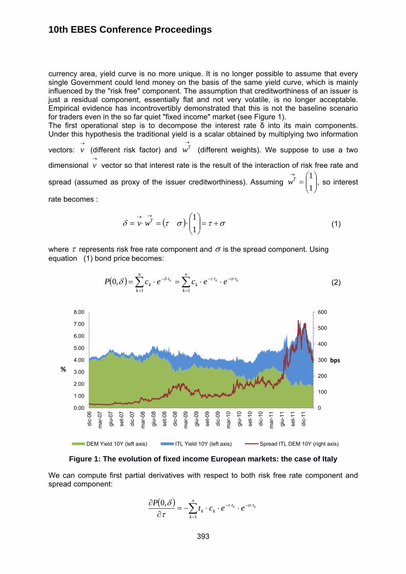
10th EBES Conference Proceedings
393
currency area, yield curve is no more unique. It is no longer possible to assume that every single Government could lend money on the basis of the same yield curve, which is mainly influenced by the "risk free" component. The assumption that creditworthiness of an issuer is just a residual component, essentially flat and not very volatile, is no longer acceptable. Empirical evidence has incontrovertibly demonstrated that this is not the baseline scenario for traders even in the so far quiet "fixed income" market (see Figure 1). The first operational step is to decompose the interest rate δ into its main components. Under this hypothesis the traditional yield is a scalar obtained by multiplying two information
vectors:
v (different risk factor) and
Tw (different weights). We suppose to use a two
dimensional
v vector so that interest rate is the result of the interaction of risk free rate and
spread (assumed as proxy of the issuer creditworthiness). Assuming
1
1Tw , so interest
rate becomes :
1
1Twv (1)
where represents risk free rate component and is the spread component. Using equation (1) bond price becomes:
n
k
ttk
n
k
tk
kkk eececP11
,0 (2)
Figure 1: The evolution of fixed income European markets: the case of Italy
We can compute first partial derivatives with respect to both risk free rate component and spread component:
n
k
ttkk
kk eectP
1
,0
0
100
200
300
400
500
600
0.00
1.00
2.00
3.00
4.00
5.00
6.00
7.00
8.00
dic-
06
mar
-07
giu-
07
set-
07
dic-
07
mar
-08
giu-
08
set-
08
dic-
08
mar
-09
giu-
09
set-
09
dic-
09
mar
-10
giu-
10
set-
10
dic-
10
mar
-11
giu-
11
set-
11
dic-
11
bps
%
DEM Yield 10Y (left axis) ITL Yield 10Y (left axis) Spread ITL DEM 10Y (right axis)

10th EBES Conference Proceedings
394
n
k
ttkk
kk eectP
1
,0
the decomposition proposed does not involve the introduction of new duration measures: “traditional” duration can be used to identify "ex ante" the impact on a bond price caused by multiple risk factors and / or to check "ex post" the effective causes leading to a given market price movement. Actually, using both Taylor expansion and the proposed decomposition in risk factors, we can write:
,0,0,0
PPPP
If we consider a yield curve, we can easily decompose the yield vector as follows:
WV
Where
represents the n-component yield vector, V is a 2n matrix (that represents the
two risk factors) and W is a 12 matrix (different weights):
21
22
11
ww
nn
kk
Under this assumption Duration (defined as the first central moment) becomes:
0,1
0,∙ ∙ ∙ ∙ ∙ ∙ ∙
Within this context, our present work will focus on the empirical impact produced by some theoretical “risk factors” on price path of bonds with the objective of verifying the soundness of the theoretical bond price decomposition we described above. Consequently, theoretical risk factors have been identified applying the building blocks approach introduced in our previous paper, with the objective of identifying both a risk free and a credit risk component. Once risk factors have been identified (see equation (2)), multiple statistical analyses have been performed in order to study how the selected risk factors may influence the price path of bonds. 2. ITALIAN GOVERNMENT BONDS: FROM THEORETIC TO EFFECTIVE RISK FACTORS We study the empirical relation between bond prices and specific potential theoretical risk factors in the Italian bond market. Government bond prices may be influenced, among others, by the following factors (Favero et al. 2007):
10th EBES Conference Proceedings
395
a) a "generic" risk free component that represents the interest paid for national debt by a country assumed to have a negligible risk of default; b) a "specific" fiscal vulnerability corresponding to the risk of default of each single country; c) the liquidity of markets where government bonds are actively traded: liquidity usually tends to vary directly with the size of the market. In large bond markets, investors can trade quickly and face a lower risk that prices will change due to individual transactions and therefore will demand less compensation in terms of the yield; d) changes in investors' preferences driving to and associated with repricing of risk: in times of heightened financial and economic uncertainty, investors typically have a higher preference for less risky and more liquid assets. This then comes with a higher premium for more risky assets as portfolio composition is adjusted to the desired new equilibrium. In particular, applying the building block approach described in §1., we are mainly interested in studying the risk-free and the credit risk component. Following Haugh et al. (2009) we use the German benchmark bund yield as a proxy for the risk-free component. More specifically, we choose the 10 years maturity bund par yield, because, among Eurozone countries, the federal republic of Germany represents, especially during recent Eurozone crisis, the effective safe investment, where risk adverse investors tend to put funds when the risk-off mood is prevailing on the market. The choice of a sound credit risk component has been more articulated. In principle, there are three types of credit risk: (i) default risk, (ii) credit spread risk and (iii) downgrade risk. The default risk is defined as the probability that the issuer fails to meet the obligations either on coupon payments or principals at maturity. Credit spread risk is the risk based on the price performance of the bond and it is defined as the probability that the market value of the bond will decline more than the value of other comparable quality bonds. Downgrade risk reflects the possibility of a downgrade by a credit rating agency (Fabozzi, 2007). The financial crisis has had an impact on all the above mentioned types of risk. The deterioration of fiscal positions due to the high cost of financial rescue packages, discretionary fiscal stimulus and the operation of automatic stabilizers raised questions about the sustainability of public finances. In addition to the usual indicators of government debt and deficit, high current account deficits in several euro area countries also heightened markets’ perception of default as these countries were considered particularly vulnerable to reversals in international flows of funding. Moreover, credit rating agencies downgraded the debt of several euro-area sovereign issuers. This may have had a direct impact on institutional investor portfolio allocation decisions, as many portfolio managers have limits on investments depending on the credit rating. Since we are interested in the relationship between price and credit risk component we refer, in particular, to the so called credit spread risk. More specifically, the credit risk component is the extra yield required to offset the expected higher loss from a given probability (usually >0%) of less than full repayment. It is important to note that credit risk includes all situations where the borrower would not be able to fully repay the loan under the initially agreed conditions. It may depend on investor assessments of the fiscal position as this affects the sustainability of the debt and the likelihood of repayment. With reference to the Eurozone, capital markets practioners dealing with Italian government bonds generally refer to the yield spread between Italian BTP and German Bund as a good empirical proxy of the credit spread risk priced in a bond price. Nevertheless, including the yield spread within a statistical framework aimed at explaining a bond price behaviour could be at last tautological because available bond yield data are generally derived from bond prices itself, driving to a kind of not acceptable auto-reference. Macroeconomic fundamentals may be considered as better
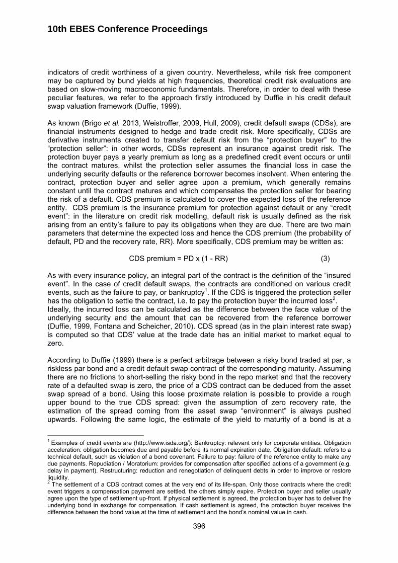
10th EBES Conference Proceedings
396
indicators of credit worthiness of a given country. Nevertheless, while risk free component may be captured by bund yields at high frequencies, theoretical credit risk evaluations are based on slow-moving macroeconomic fundamentals. Therefore, in order to deal with these peculiar features, we refer to the approach firstly introduced by Duffie in his credit default swap valuation framework (Duffie, 1999). As known (Brigo et al. 2013, Weistroffer, 2009, Hull, 2009), credit default swaps (CDSs), are financial instruments designed to hedge and trade credit risk. More specifically, CDSs are derivative instruments created to transfer default risk from the “protection buyer” to the “protection seller”: in other words, CDSs represent an insurance against credit risk. The protection buyer pays a yearly premium as long as a predefined credit event occurs or until the contract matures, whilst the protection seller assumes the financial loss in case the underlying security defaults or the reference borrower becomes insolvent. When entering the contract, protection buyer and seller agree upon a premium, which generally remains constant until the contract matures and which compensates the protection seller for bearing the risk of a default. CDS premium is calculated to cover the expected loss of the reference entity. CDS premium is the insurance premium for protection against default or any “credit event”: in the literature on credit risk modelling, default risk is usually defined as the risk arising from an entity’s failure to pay its obligations when they are due. There are two main parameters that determine the expected loss and hence the CDS premium (the probability of default, PD and the recovery rate, RR). More specifically, CDS premium may be written as:
CDS premium = PD x (1 - RR) (3) As with every insurance policy, an integral part of the contract is the definition of the “insured event”. In the case of credit default swaps, the contracts are conditioned on various credit events, such as the failure to pay, or bankruptcy1. If the CDS is triggered the protection seller has the obligation to settle the contract, i.e. to pay the protection buyer the incurred loss2. Ideally, the incurred loss can be calculated as the difference between the face value of the underlying security and the amount that can be recovered from the reference borrower (Duffie, 1999, Fontana and Scheicher, 2010). CDS spread (as in the plain interest rate swap) is computed so that CDS’ value at the trade date has an initial market to market equal to zero. According to Duffie (1999) there is a perfect arbitrage between a risky bond traded at par, a riskless par bond and a credit default swap contract of the corresponding maturity. Assuming there are no frictions to short-selling the risky bond in the repo market and that the recovery rate of a defaulted swap is zero, the price of a CDS contract can be deduced from the asset swap spread of a bond. Using this loose proximate relation is possible to provide a rough upper bound to the true CDS spread: given the assumption of zero recovery rate, the estimation of the spread coming from the asset swap “environment” is always pushed upwards. Following the same logic, the estimate of the yield to maturity of a bond is at a
1 Examples of credit events are (http://www.isda.org/): Bankruptcy: relevant only for corporate entities. Obligation acceleration: obligation becomes due and payable before its normal expiration date. Obligation default: refers to a technical default, such as violation of a bond covenant. Failure to pay: failure of the reference entity to make any due payments. Repudiation / Moratorium: provides for compensation after specified actions of a government (e.g. delay in payment). Restructuring: reduction and renegotiation of delinquent debts in order to improve or restore liquidity. 2 The settlement of a CDS contract comes at the very end of its life-span. Only those contracts where the credit event triggers a compensation payment are settled, the others simply expire. Protection buyer and seller usually agree upon the type of settlement up-front. If physical settlement is agreed, the protection buyer has to deliver the underlying bond in exchange for compensation. If cash settlement is agreed, the protection buyer receives the difference between the bond value at the time of settlement and the bond’s nominal value in cash.

10th EBES Conference Proceedings
397
lower level compared with the “true” one, since we do not consider the cost associated with shorting the risky asset. Under these assumptions, the annual yield of a risk free bond must be in equilibrium with the difference between the annual yield of the corresponding risky bond and the cost of credit protection expressed as a percentage of the risky bond nominal value (see equation (4)).
BY (risk free) = BY – CDS (spread) (4) In order to identify possible market data suitable to explain the effective sovereign bond price behaviour, we therefore choose to refer to the credit default swap (CDS) on sovereigns.
Like most CDS contracts, sovereign CDS typically serve as trading instruments rather than pure insurance instruments3. In addition to country default risk, a number of additional factors may influence the information content of CDS premium. In relative terms, sovereign CDS volume is small. Only the worsening of the current crisis pointed out the attention to default risk in euro area sovereign debt, and, consequently, for trading and for hedging reasons, market activity in euro area sovereign CDS has grown strongly. Sovereign CDS on e.g. euro governments are typically denominated in US$. One reason for choosing a different currency than the bond’s original denomination is that this allows investors to avoid the risk of a severe depreciation of the bond’s currency in case of a credit event. This currency mismatch introduces an element of exchange rate risk into the pricing of the contract. Counterparty risk may matter far more for sovereign CDS than for corporate CDS. In particular, CDS on major countries may not always provide genuinely robust insurance against a large-scale default given the close linkages between sovereigns and the financial sector. Since, as we mentioned above, the objective of the present work is to analyse how the credit risk component may influence the market price of government bonds, we were forced to refer to the CDS on the Republic of Italy. Nonetheless it is interesting to refer to recent empirical studies (Barrios et al. 2009) aimed at understanding the role of both government bonds and CDS contracts in the proper market pricing of the effective credit risk level of a single State. In this context, Palladini and Portes (2011) pointed out that there is clear evidence that CDS and bond yield spreads diverge substantially in the short run. Their Vector Error Correction Model (VECM) results suggest that this may be attributed largely to a different timing of response to new information available in the short run. Nonetheless, their cointegration analysis supports the long-run price accuracy of CDS relative to the underlying bond market, suggesting long-run equilibrium between the two credit prices. Once main risk factors have been identified, a multiple regression analysis has been performed with the aim of verifying the role played by each risk factor in the explanation of the whole bond price variation. We start considering a fixed rate bond, namely the Italian “BtP” with maturity of about 10 years. We focus on the ten-year horizon as this is the common horizon for the government bond. Hence, our price data cover benchmark bonds with a ten-year maturity. More specifically, we build the 10y BTP historical series taking into account the so called “benchmark” bond, generally considered as the more liquid bond for a given maturity at a given time in the secondary market. In particular, starting from the closing prices of the bond listed in Table 1 we build a 5years time series of a BTP 10y rolling benchmark bond represented in Figure 2. We create the BTP rolling by daily historical prices.
3 Investors commonly use sovereign CDS for the following purposes: taking an outright position on spreads depending on traders’ expectations over a short horizon; hedging macro, i.e. country risk (e.g. a bank’s exposure to a quasi-governmental body); relative-value trading (e.g. a short position in country X and a long position in country Y); arbitrage trading (e.g. government bonds vs. CDS).
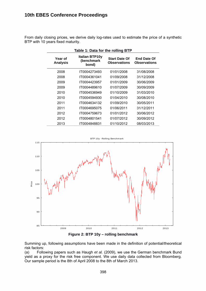
10th EBES Conference Proceedings
398
From daily closing prices, we derive daily log-rates used to estimate the price of a synthetic BTP with 10 years fixed maturity.
Table 1: Data for the rolling BTP
Year of Analysis
Italian BTP10y (benchmark
bond)
Start Date Of Observations
End Date Of Observations
2008 IT0004273493 01/01/2008 31/08/2008
2008 IT0004361041 01/09/2008 31/12/2008
2009 IT0004423957 01/01/2009 30/06/2009
2009 IT0004489610 01/07/2009 30/09/2009
2010 IT0004536949 01/10/2009 31/03/2010
2010 IT0004594930 01/04/2010 30/08/2010
2011 IT0004634132 01/09/2010 30/05/2011
2011 IT0004695075 01/06/2011 31/12/2011
2012 IT0004759673 01/01/2012 30/06/2012
2012 IT0004801541 01/07/2012 30/09/2012
2013 IT0004848831 01/10/2012 08/03/2013
Figure 2: BTP 10y – rolling benchmark
Summing up, following assumptions have been made in the definition of potential/theoretical risk factors: (a) Following papers such as Haugh et al. (2009), we use the German benchmark Bund yield as a proxy for the risk free component. We use daily data collected from Bloomberg. Our sample period is the 8th of April 2008 to the 8th of March 2013.
85
90
95
100
105
110
115
2009 2010 2011 2012 2013
Pri
ce
BTP 10y -Rolling Benchmark
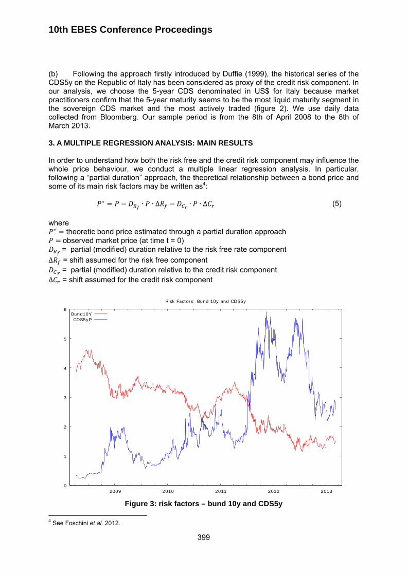
10th EBES Conference Proceedings
399
(b) Following the approach firstly introduced by Duffie (1999), the historical series of the CDS5y on the Republic of Italy has been considered as proxy of the credit risk component. In our analysis, we choose the 5-year CDS denominated in US$ for Italy because market practitioners confirm that the 5-year maturity seems to be the most liquid maturity segment in the sovereign CDS market and the most actively traded (figure 2). We use daily data collected from Bloomberg. Our sample period is from the 8th of April 2008 to the 8th of March 2013. 3. A MULTIPLE REGRESSION ANALYSIS: MAIN RESULTS In order to understand how both the risk free and the credit risk component may influence the whole price behaviour, we conduct a multiple linear regression analysis. In particular, following a “partial duration” approach, the theoretical relationship between a bond price and some of its main risk factors may be written as4:
∗ ∙ ∙ ∆ ∙ ∙ ∆ (5)
where ∗ theoretic bond price estimated through a partial duration approach observed market price (at time t = 0) = partial (modified) duration relative to the risk free rate component
∆ = shift assumed for the risk free component = partial (modified) duration relative to the credit risk component
∆ = shift assumed for the credit risk component
Figure 3: risk factors – bund 10y and CDS5y
4 See Foschini et al. 2012.
0
1
2
3
4
5
6
2009 2010 2011 2012 2013
Risk Factors: Bund 10y and CDS5y
Bund10YCDS5yP
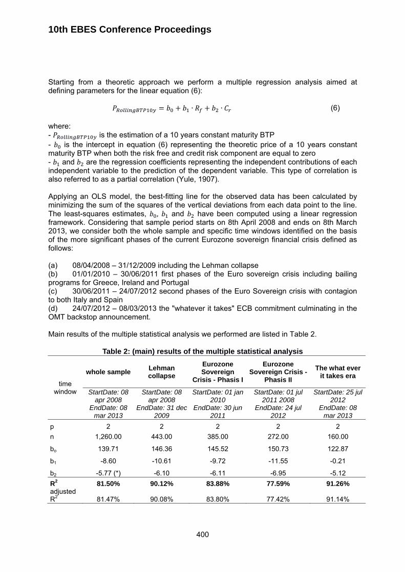
10th EBES Conference Proceedings
400
Starting from a theoretic approach we perform a multiple regression analysis aimed at defining parameters for the linear equation (6):
∙ ∙ (6) where: - is the estimation of a 10 years constant maturity BTP - is the intercept in equation (6) representing the theoretic price of a 10 years constant maturity BTP when both the risk free and credit risk component are equal to zero - and are the regression coefficients representing the independent contributions of each independent variable to the prediction of the dependent variable. This type of correlation is also referred to as a partial correlation (Yule, 1907). Applying an OLS model, the best-fitting line for the observed data has been calculated by minimizing the sum of the squares of the vertical deviations from each data point to the line. The least-squares estimates, , and have been computed using a linear regression framework. Considering that sample period starts on 8th April 2008 and ends on 8th March 2013, we consider both the whole sample and specific time windows identified on the basis of the more significant phases of the current Eurozone sovereign financial crisis defined as follows: (a) 08/04/2008 – 31/12/2009 including the Lehman collapse (b) 01/01/2010 – 30/06/2011 first phases of the Euro sovereign crisis including bailing programs for Greece, Ireland and Portugal (c) 30/06/2011 – 24/07/2012 second phases of the Euro Sovereign crisis with contagion to both Italy and Spain (d) 24/07/2012 – 08/03/2013 the "whatever it takes" ECB commitment culminating in the OMT backstop announcement. Main results of the multiple statistical analysis we performed are listed in Table 2.
Table 2: (main) results of the multiple statistical analysis
time window
whole sample Lehman collapse
Eurozone Sovereign
Crisis - Phasis I
Eurozone Sovereign Crisis -
Phasis II
The what ever it takes era
StartDate: 08 apr 2008
StartDate: 08 apr 2008
StartDate: 01 jan 2010
StartDate: 01 jul 2011 2008
StartDate: 25 jul 2012
EndDate: 08 mar 2013
EndDate: 31 dec 2009
EndDate: 30 jun 2011
EndDate: 24 jul 2012
EndDate: 08 mar 2013
p 2 2 2 2 2
n 1,260.00 443.00 385.00 272.00 160.00
bo 139.71 146.36 145.52 150.73 122.87
b1 -8.60 -10.61 -9.72 -11.55 -0.21
b2 -5.77 (*) -6.10 -6.11 -6.95 -5.12
R2 81.50% 90.12% 83.88% 77.59% 91.26% adjusted R2 81.47% 90.08% 83.80% 77.42% 91.14%
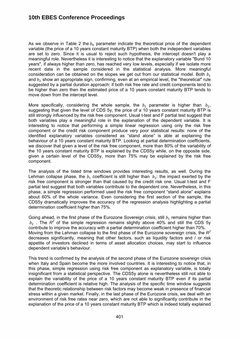
10th EBES Conference Proceedings
401
As we observe in Table 2 the parameter indicate the theoretical price of the dependent variable (the price of a 10 years constant maturity BTP) when both the independent variables are set to zero. Since it is usual to reject such hypothesis, the intercept doesn't play a meaningful role. Nevertheless it is interesting to notice that the explanatory variable "Bund 10 years", if always higher than zero, has reached very low levels, especially if we isolate more recent data in the sample considered in the statistical analysis. More meaningful consideration can be obtained on the slopes we get out from our statistical model. Both and show an appropriate sign, confirming, even at an empirical level, the "theoretical" rule suggested by a partial duration approach: if both risk free rate and credit components tend to be higher than zero then the estimated price of a 10 years constant maturity BTP tends to move down from the intercept level. More specifically, considering the whole sample, the parameter is higher than , suggesting that given the level of CDS 5y, the price of a 10 years constant maturity BTP is still strongly influenced by the risk free component. Usual t-test and F partial test suggest that both variables play a meaningful role in the explanation of the dependent variable. It is interesting to notice that performing a simple linear regression using only the risk free component or the credit risk component produce very poor statistical results: none of the identified explanatory variables considered as “stand alone” is able at explaining the behaviour of a 10 years constant maturity BTP. Looking at partial determination coefficients, we discover that given a level of the risk free component, more than 80% of the variability of the 10 years constant maturity BTP is explained by the CDS5y while, on the opposite side, given a certain level of the CDS5y, more than 75% may be explained by the risk free component. The analysis of the listed time windows provides interesting results, as well. During the Lehman collapse phase, the coefficient is still higher than : the impact exerted by the risk free component is stronger than that caused by the credit risk one. Usual t-test and F partial test suggest that both variables contribute to the dependent one. Nevertheless, in this phase, a simple regression performed used the risk free component “stand alone” explains about 60% of the whole variance. Even considering the first section of the sample, the CDS5y dramatically improves the accuracy of the regression analysis highlighting a partial determination coefficient higher than 75%. Going ahead, in the first phase of the Eurozone Sovereign crisis, still remains higher than . The R2 of the simple regression remains slightly above 40% and still the CDS 5y contribute to improve the accuracy with a partial determination coefficient higher than 70%. Moving from the Lehman collapse to the first phase of the Eurozone sovereign crisis, the R2 decreases significantly, meaning that other factors, such as liquidity factors and / or risk appetite of investors declined in terms of asset allocation choices, may start to influence dependent variable’s behaviour. This trend is confirmed by the analysis of the second phase of the Eurozone sovereign crisis when Italy and Spain become the more involved countries. It is interesting to notice that, in this phase, simple regression using risk free component as explanatory variable, is totally insignificant from a statistical perspective. The CDS5y alone is nevertheless still not able to explain the variability of the price of a 10 years constant maturity BTP even if its partial determination coefficient is relative high. The analysis of the specific time window suggests that the theoretic relationship between risk factors may become weak in presence of financial stress within a given market. Finally, in the last phase of the Eurozone crisis, we deal with an environment of risk free rates near zero, which are not able to significantly contribute in the explanation of the price of a 10 years constant maturity BTP which is indeed totally explained
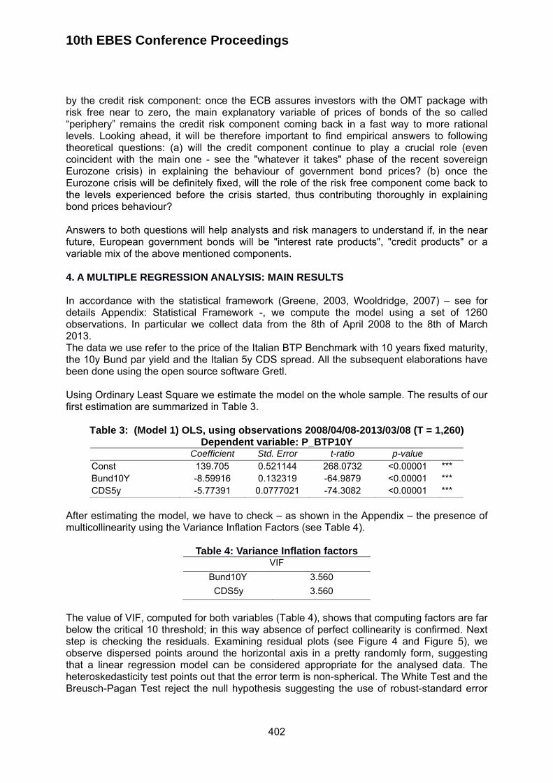
10th EBES Conference Proceedings
402
by the credit risk component: once the ECB assures investors with the OMT package with risk free near to zero, the main explanatory variable of prices of bonds of the so called “periphery” remains the credit risk component coming back in a fast way to more rational levels. Looking ahead, it will be therefore important to find empirical answers to following theoretical questions: (a) will the credit component continue to play a crucial role (even coincident with the main one - see the "whatever it takes" phase of the recent sovereign Eurozone crisis) in explaining the behaviour of government bond prices? (b) once the Eurozone crisis will be definitely fixed, will the role of the risk free component come back to the levels experienced before the crisis started, thus contributing thoroughly in explaining bond prices behaviour? Answers to both questions will help analysts and risk managers to understand if, in the near future, European government bonds will be "interest rate products", "credit products" or a variable mix of the above mentioned components. 4. A MULTIPLE REGRESSION ANALYSIS: MAIN RESULTS In accordance with the statistical framework (Greene, 2003, Wooldridge, 2007) – see for details Appendix: Statistical Framework -, we compute the model using a set of 1260 observations. In particular we collect data from the 8th of April 2008 to the 8th of March 2013. The data we use refer to the price of the Italian BTP Benchmark with 10 years fixed maturity, the 10y Bund par yield and the Italian 5y CDS spread. All the subsequent elaborations have been done using the open source software Gretl. Using Ordinary Least Square we estimate the model on the whole sample. The results of our first estimation are summarized in Table 3.
Table 3: (Model 1) OLS, using observations 2008/04/08-2013/03/08 (T = 1,260) Dependent variable: P_BTP10Y
Coefficient Std. Error t-ratio p-value Const 139.705 0.521144 268.0732 <0.00001 *** Bund10Y -8.59916 0.132319 -64.9879 <0.00001 *** CDS5y -5.77391 0.0777021 -74.3082 <0.00001 ***
After estimating the model, we have to check – as shown in the Appendix – the presence of multicollinearity using the Variance Inflation Factors (see Table 4).
Table 4: Variance Inflation factors VIF
Bund10Y 3.560
CDS5y 3.560
The value of VIF, computed for both variables (Table 4), shows that computing factors are far below the critical 10 threshold; in this way absence of perfect collinearity is confirmed. Next step is checking the residuals. Examining residual plots (see Figure 4 and Figure 5), we observe dispersed points around the horizontal axis in a pretty randomly form, suggesting that a linear regression model can be considered appropriate for the analysed data. The heteroskedasticity test points out that the error term is non-spherical. The White Test and the Breusch-Pagan Test reject the null hypothesis suggesting the use of robust-standard error
10th EBES Conference Proceedings
403
estimators, as shown in Table 5. The results obtained using the OLS Robust standard errors are summarized in Table 6. The computed coefficients are extremely similar in both models; the value referred to standard errors and t-ratio are different due to the fact that we adjust computations with the weighted covariance matrix of the error terms, as defined in the White Estimators. The main result of using robust standard errors is the enhancement of the test statistics we use for inference.
Figure 4: Bund 10y regression residuals
Table 5: Heteroskedasticity Test White's test (squares only) Breusch-Pagan test
Null hypothesis: heteroskedasticity not present
Null hypothesis: heteroskedasticity not present
Test statistic: LM = 134.087 Test statistic: LM = 59.1677
with p-value = P(Chi-square(4) > 134.087) = 5.20225e-028
with p-value = P(Chi-square(2) > 59.1677) = 1.41873e-013
The significance of each variable is confirmed by t-ratio; the joint significance of the model can be evaluated analysing F statistic. In both cases the corresponding p-value is close to zero. The intercept corresponding to the value of the price of BTP10y rolling benchmark if both the independent variables are equal to zero: in our base case, and in the whole sample, the value of the intercept is 139.705. Regression coefficients represent the independent contributions of each explanatory variable. It is interesting to note that the independent contribution of the risk free component is similar to that usually expressed by a modified duration of a 10 year risk free note. Even the partial effect produced by CDS 5Y on the dependent variable looks similar to a modified duration of a 10 years fixed rate bond. It is
-6
-4
-2
0
2
4
6
1.5 2 2.5 3 3.5 4 4.5
resi
dual
Bund10Y
Bund10Y Regression residuals (= observed - fitted P_BTP10Y)
10th EBES Conference Proceedings
404
important to notice that the effect of CDS 5y is smaller than the one produced by the risk free component. The R2 commonly used to evaluate model fit, is 81.50%, meaning that the model explains more than 80% of the original variability; this indicates that we account for almost all of the variability with the variables specified in the model. The Adjusted R-square (81.47%) built taking into account the number of sample observations (n=1260) and the number of explanatory variables (p=2) still indicates that the model explains more than 80% of the original variability. The actual and fitted values are shown in Figure 6.
Figure 5: CDS5y regression residuals
Table 6: (Model 2): OLS, using observations 2008/04/08-2013/03/08 (T = 1,260) Dependent variable: P_BTP10Y
Heteroskedasticity-robust standard errors, variant HC0 Coefficient Std. Error t-ratio p-value
const 139.705 0.650273 214.8398 <0.00001 *** Bund10Y -8.59916 0.164424 -52.2987 <0.00001 *** CDS5y -5.77391 0.0897895 -64.3049 <0.00001 *** Mean dependent var 103.3257 S.D. dependent var 5.082955Sum squared resid 6,019.464 S.E. of regression 2.188322R-squared 0.814945 Adjusted R-squared 0.814651F(2, 1257) 2,129.490 P-value(F) 0.000000
-6
-4
-2
0
2
4
6
1 2 3 4 5 6
resi
dual
CDS5y
CDS 5y Regression residuals (= observed - fitted P_BTP10Y)
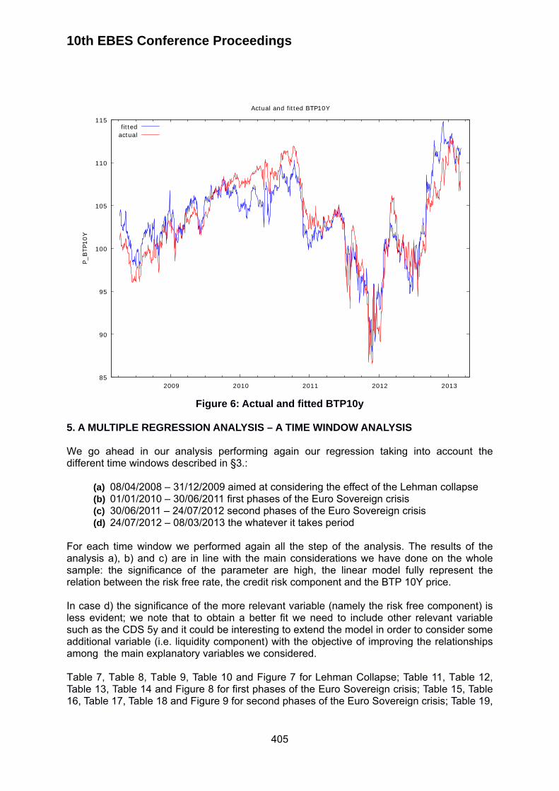
10th EBES Conference Proceedings
405
Figure 6: Actual and fitted BTP10y
5. A MULTIPLE REGRESSION ANALYSIS – A TIME WINDOW ANALYSIS We go ahead in our analysis performing again our regression taking into account the different time windows described in §3.:
(a) 08/04/2008 – 31/12/2009 aimed at considering the effect of the Lehman collapse (b) 01/01/2010 – 30/06/2011 first phases of the Euro Sovereign crisis (c) 30/06/2011 – 24/07/2012 second phases of the Euro Sovereign crisis (d) 24/07/2012 – 08/03/2013 the whatever it takes period
For each time window we performed again all the step of the analysis. The results of the analysis a), b) and c) are in line with the main considerations we have done on the whole sample: the significance of the parameter are high, the linear model fully represent the relation between the risk free rate, the credit risk component and the BTP 10Y price. In case d) the significance of the more relevant variable (namely the risk free component) is less evident; we note that to obtain a better fit we need to include other relevant variable such as the CDS 5y and it could be interesting to extend the model in order to consider some additional variable (i.e. liquidity component) with the objective of improving the relationships among the main explanatory variables we considered. Table 7, Table 8, Table 9, Table 10 and Figure 7 for Lehman Collapse; Table 11, Table 12, Table 13, Table 14 and Figure 8 for first phases of the Euro Sovereign crisis; Table 15, Table 16, Table 17, Table 18 and Figure 9 for second phases of the Euro Sovereign crisis; Table 19,
85
90
95
100
105
110
115
2009 2010 2011 2012 2013
P_BTP
10Y
Actual and fitted BTP10Y
fittedactual
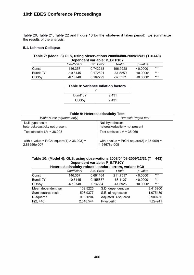
10th EBES Conference Proceedings
406
Table 20, Table 21, Table 22 and Figure 10 for the whatever it takes period) we summarize the results of the analysis. 5.1. Lehman Collapse
Table 7: (Model 3) OLS, using observations 2008/04/08-2009/12/31 (T = 443)
Dependent variable: P_BTP10Y Coefficient Std. Error t-ratio p-value
Const 146.357 0.743218 196.9228 <0.00001 *** Bund10Y -10.6145 0.172521 -61.5259 <0.00001 *** CDS5y -6.10748 0.162792 -37.5171 <0.00001 ***
Table 8: Variance Inflation factors
VIF
Bund10Y 2.431
CDS5y 2.431
Table 9: Heteroskedasticity Test White's test (squares only) Breusch-Pagan test
Null hypothesis: heteroskedasticity not present
Null hypothesis: heteroskedasticity not present
Test statistic: LM = 36.003 Test statistic: LM = 35.969
with p-value = P(Chi-square(4) > 36.003) = 2.88956e-007
with p-value = P(Chi-square(2) > 35.969) = 1.54678e-008
Table 10: (Model 4): OLS, using observations 2008/04/08-2009/12/31 (T = 443) Dependent variable: P_BTP10Y
Heteroskedasticity-robust standard errors, variant HC0 Coefficient Std. Error t-ratio p-value
Const 146.357 0.691164 211.7537 <0.00001 *** Bund10Y -10.6145 0.155837 -68.1127 <0.00001 *** CDS5y -6.10748 0.14684 -41.5926 <0.00001 *** Mean dependent var 102.5225 S.D. dependent var 3.413900Sum squared resid 508.9377 S.E. of regression 1.075489R-squared 0.901204 Adjusted R-squared 0.900755F(2, 440) 2,518.544 P-value(F) 1.2e-241
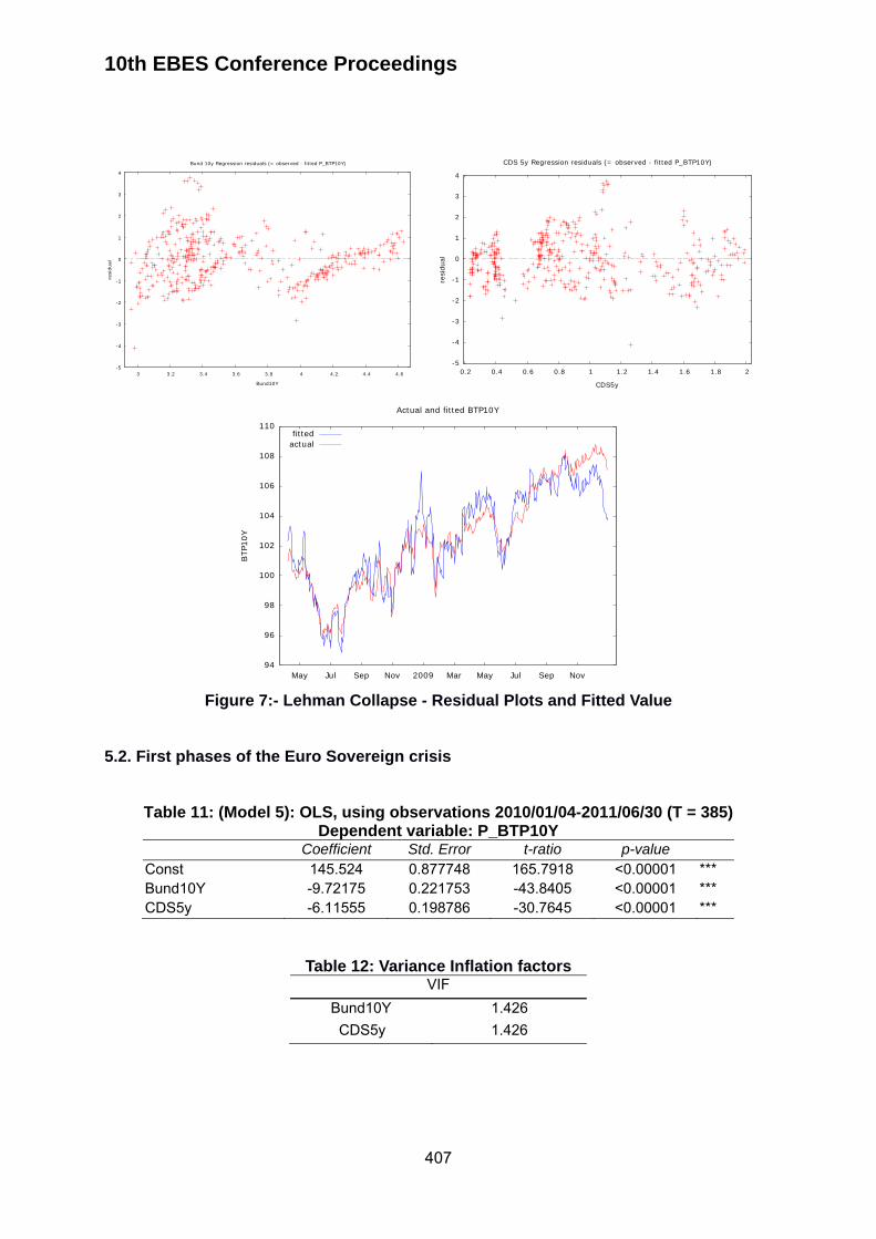
10th EBES Conference Proceedings
407
Figure 7:- Lehman Collapse - Residual Plots and Fitted Value
5.2. First phases of the Euro Sovereign crisis
Table 11: (Model 5): OLS, using observations 2010/01/04-2011/06/30 (T = 385) Dependent variable: P_BTP10Y
Coefficient Std. Error t-ratio p-value Const 145.524 0.877748 165.7918 <0.00001 *** Bund10Y -9.72175 0.221753 -43.8405 <0.00001 *** CDS5y -6.11555 0.198786 -30.7645 <0.00001 ***
Table 12: Variance Inflation factors VIF
Bund10Y 1.426
CDS5y 1.426
-5
-4
-3
-2
-1
0
1
2
3
4
3 3.2 3.4 3.6 3.8 4 4.2 4.4 4.6
resi
dual
Bund10Y
Bund 10y Regression residuals (= observed - fitted P_BTP10Y)
-5
-4
-3
-2
-1
0
1
2
3
4
0.2 0.4 0.6 0.8 1 1.2 1.4 1.6 1.8 2
resi
dual
CDS5y
CDS 5y Regression residuals (= observed - fitted P_BTP10Y)
94
96
98
100
102
104
106
108
110
May Jul Sep Nov 2009 Mar May Jul Sep Nov
BTP
10Y
Actual and fitted BTP10Y
fittedactual
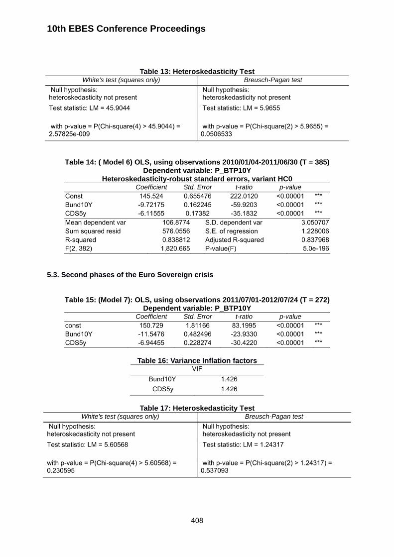
10th EBES Conference Proceedings
408
Table 13: Heteroskedasticity Test White's test (squares only) Breusch-Pagan test
Null hypothesis: heteroskedasticity not present
Null hypothesis: heteroskedasticity not present
Test statistic: LM = 45.9044 Test statistic: LM = 5.9655
with p-value = P(Chi-square(4) > 45.9044) = 2.57825e-009
with p-value = P(Chi-square(2) > 5.9655) = 0.0506533
Table 14: ( Model 6) OLS, using observations 2010/01/04-2011/06/30 (T = 385) Dependent variable: P_BTP10Y
Heteroskedasticity-robust standard errors, variant HC0 Coefficient Std. Error t-ratio p-value
Const 145.524 0.655476 222.0120 <0.00001 *** Bund10Y -9.72175 0.162245 -59.9203 <0.00001 *** CDS5y -6.11555 0.17382 -35.1832 <0.00001 *** Mean dependent var 106.8774 S.D. dependent var 3.050707Sum squared resid 576.0556 S.E. of regression 1.228006R-squared 0.838812 Adjusted R-squared 0.837968F(2, 382) 1,820.665 P-value(F) 5.0e-196
5.3. Second phases of the Euro Sovereign crisis
Table 15: (Model 7): OLS, using observations 2011/07/01-2012/07/24 (T = 272) Dependent variable: P_BTP10Y
Coefficient Std. Error t-ratio p-value const 150.729 1.81166 83.1995 <0.00001 *** Bund10Y -11.5476 0.482496 -23.9330 <0.00001 *** CDS5y -6.94455 0.228274 -30.4220 <0.00001 ***
Table 16: Variance Inflation factors
VIF
Bund10Y 1.426
CDS5y 1.426
Table 17: Heteroskedasticity Test
White's test (squares only) Breusch-Pagan test
Null hypothesis: heteroskedasticity not present
Null hypothesis: heteroskedasticity not present
Test statistic: LM = 5.60568 Test statistic: LM = 1.24317
with p-value = P(Chi-square(4) > 5.60568) = 0.230595
with p-value = P(Chi-square(2) > 1.24317) = 0.537093
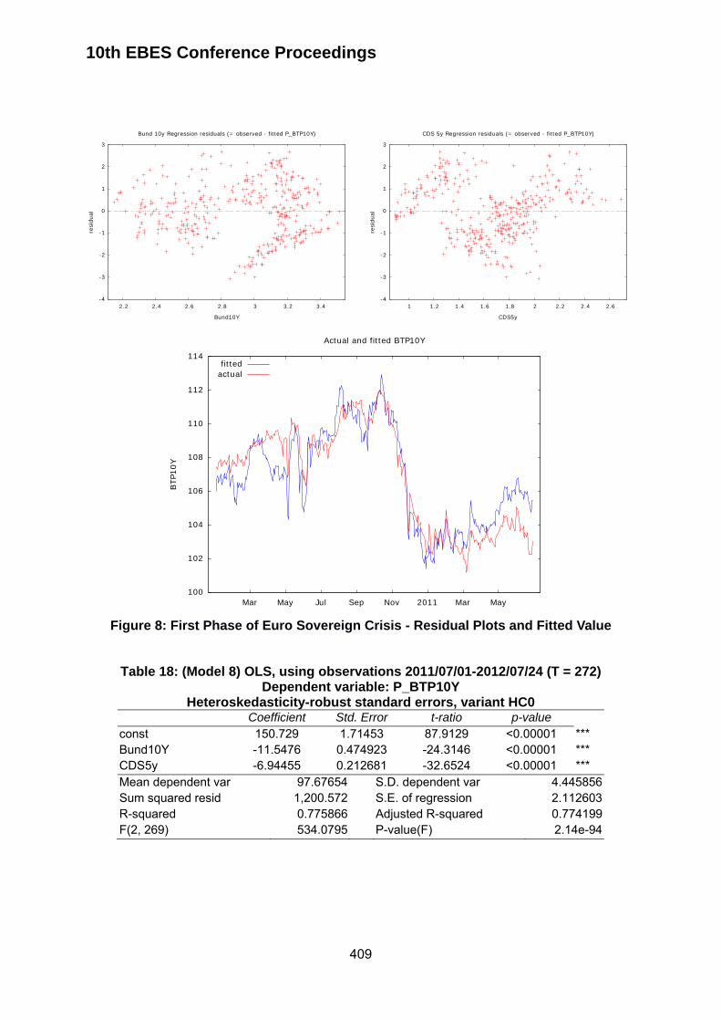
10th EBES Conference Proceedings
409
Figure 8: First Phase of Euro Sovereign Crisis - Residual Plots and Fitted Value
Table 18: (Model 8) OLS, using observations 2011/07/01-2012/07/24 (T = 272) Dependent variable: P_BTP10Y
Heteroskedasticity-robust standard errors, variant HC0 Coefficient Std. Error t-ratio p-value
const 150.729 1.71453 87.9129 <0.00001 *** Bund10Y -11.5476 0.474923 -24.3146 <0.00001 *** CDS5y -6.94455 0.212681 -32.6524 <0.00001 *** Mean dependent var 97.67654 S.D. dependent var 4.445856Sum squared resid 1,200.572 S.E. of regression 2.112603R-squared 0.775866 Adjusted R-squared 0.774199F(2, 269) 534.0795 P-value(F) 2.14e-94
-4
-3
-2
-1
0
1
2
3
2.2 2.4 2.6 2.8 3 3.2 3.4
resi
dual
Bund10Y
Bund 10y Regression residuals (= observed - fitted P_BTP10Y)
-4
-3
-2
-1
0
1
2
3
1 1.2 1.4 1.6 1.8 2 2.2 2.4 2.6
resi
dual
CDS5y
CDS 5y Regression residuals (= observed - fitted P_BTP10Y)
100
102
104
106
108
110
112
114
Mar May Jul Sep Nov 2011 Mar May
BTP
10Y
Actual and fitted BTP10Y
fittedactual
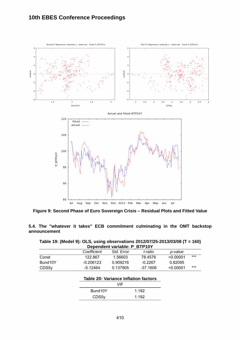
10th EBES Conference Proceedings
410
Figure 9: Second Phase of Euro Sovereign Crisis – Residual Plots and Fitted Value
5.4. The "whatever it takes" ECB commitment culminating in the OMT backstop announcement
Table 19: (Model 9): OLS, using observations 2012/07/25-2013/03/08 (T = 160)
Dependent variable: P_BTP10Y Coefficient Std. Error t-ratio p-value
Const 122.867 1.56603 78.4576 <0.00001 *** Bund10Y -0.206123 0.909216 -0.2267 0.82095 CDS5y -5.12464 0.137905 -37.1606 <0.00001 ***
Table 20: Variance Inflation factors
VIF
Bund10Y 1.192
CDS5y 1.192
-6
-4
-2
0
2
4
6
1.5 2 2.5 3
resi
dual
Bund10Y
Bund10Y Regression residuals (= observed - fitted P_BTP10Y)
-6
-4
-2
0
2
4
6
2 2.5 3 3.5 4 4.5 5 5.5 6
resi
dual
CDS5y
CDS 5Y Regression residuals (= observed - fitted P_BTP10Y)
85
90
95
100
105
110
Jul Aug Sep Oct Nov Dec 2012 Feb Mar Apr May Jun Jul
P_BTP
10Y
Actual and fitted BTP10Y
fittedactual

10th EBES Conference Proceedings
411
Table 21: Heteroskedasticity Test White's test (squares only) Breusch-Pagan test
Null hypothesis: heteroskedasticity not present
Null hypothesis: heteroskedasticity not present
Test statistic: LM = 39.2978 Test statistic: LM = 15.9321
with p-value = P(Chi-square(4) > 39.2978) = 6.04632e-008
with p-value = P(Chi-square(2) > 15.9321) = 0.000347045
Table 22: (Model 10): OLS, using observations 2012/07/25-2013/03/08 (T = 160)
Dependent variable: P_BTP10Y Heteroskedasticity-robust standard errors, variant HC0
Coefficient Std. Error t-ratio p-value const 122.867 1.24914 98.3611 <0.00001 *** Bund10Y -0.206123 0.78965 -0.2610 0.79441 CDS5y -5.12464 0.114701 -44.6784 <0.00001 *** Mean dependent var 106.6071 S.D. dependent var 4.271351Sum squared resid 253.6610 S.E. of regression 1.271092R-squared 0.912557 Adjusted R-squared 0.911443F(2, 157) 1,011.819 P-value(F) 1.99e-90
6. CONCLUSIONS AND FURTHER WORKS The present work starts from the paper "Small partial duration grow" (Foschini et al. 2012) aimed at enriching the capital markets practitioners toolbox, defining a "new" set of sensitivity measures, that, starting from the “partial derivatives” approach embedded in the traditional duration framework could help analysts and risk managers in understanding some of the more relevant drivers of a fixed income portfolio behavior. Applying such a framework, our present work studied the empirical impact produced by some theoretical “risk factors” on price path of bonds with the objective of verifying the soundness and the suitability of the theoretical bond price decomposition introduced in our previous paper. We refer in particular to the Italian bond market and we study the empirical relation between bond prices and risk free and a credit risk components, identified as theoretical risk factors. More specifically: the German benchmark Bund yield - following Haugh et al. (2009) - has been chosen as proxy for the risk free component while the CDS5y on the Republic of Italy has been considered as proxy of the credit risk component - following Duffie (1999). Once risk factors have been defined, multiple statistical analysis has been performed in order to analyze how selected risk factors influence the price path of bonds. We use daily data collected from Bloomberg. Considering that sample period starts on 8th April 2008 and ends on 8th March 2013, we consider both the whole sample and specific time windows identified on the basis of the more significant phases of the current Eurozone sovereign financial crisis. Looking at the whole sample, empirical results confirm the "theoretical" rule suggested by a partial duration approach: if both risk free rate and credit components tend to be higher than zero then the estimated price of a government bond tend to move down from the intercept level, representing only a theoretic price when both risk free and credit risk component are null. Going into specific "time windows", a comprehensive explanation of a given price path of bonds reveals on one side an increasing weakness of the risk free component and on the other side an increasing weight of the credit component culminating in the more recent phases of the Eurozone Crisis. Looking ahead, it will be therefore important to find empirical
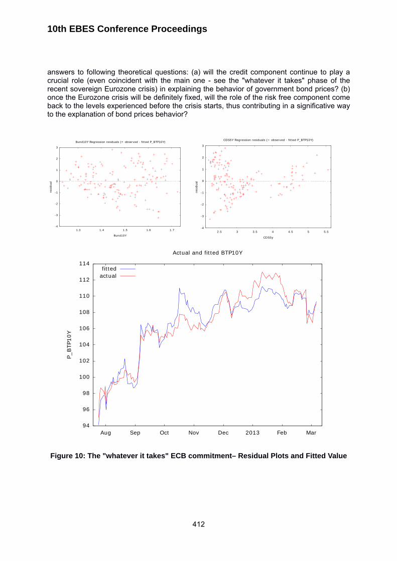
10th EBES Conference Proceedings
412
answers to following theoretical questions: (a) will the credit component continue to play a crucial role (even coincident with the main one - see the "whatever it takes" phase of the recent sovereign Eurozone crisis) in explaining the behavior of government bond prices? (b) once the Eurozone crisis will be definitely fixed, will the role of the risk free component come back to the levels experienced before the crisis starts, thus contributing in a significative way to the explanation of bond prices behavior?
Figure 10: The "whatever it takes" ECB commitment– Residual Plots and Fitted Value
-4
-3
-2
-1
0
1
2
3
1.3 1.4 1.5 1.6 1.7
resi
dual
Bund10Y
Bund10Y Regression residuals (= observed - fitted P_BTP10Y)
-4
-3
-2
-1
0
1
2
3
2.5 3 3.5 4 4.5 5 5.5
resi
dual
CDS5y
CDS5Y Regression residuals (= observed - fitted P_BTP10Y)
94
96
98
100
102
104
106
108
110
112
114
Aug Sep Oct Nov Dec 2013 Feb Mar
P_BTP
10Y
Actual and fitted BTP10Y
fittedactual

10th EBES Conference Proceedings
413
Answers to both above identified questions will help analysts and risk managers to understand if, in the near future, European government bonds will be "interest rate products", "credit products" or a variable mix of the above mentioned components. From a statistical perspective it will be interesting to improve the statistical model we used in present work with the objective of enriching the set of independent variables including aspects able at capturing, i.e. the liquidity component and / or other suitable factors. (see for example the second phases of the Euro Sovereign crisis with contagion to both Italy and Spain where the R2 reaches its minimum level or the "whatever it takes phase when the credit component remains the only empirical effective independent variable of the model). REFERENCES
Barrios, S., Iversen, P., Lewandowska, M., and Setzer, R. 2009. Determinants of intra-euro area government bond spreads during the financial crisis. Economic Papers European Economy, 388. Brigo, D., Morini, M., and Pallavicini, A., 2013. Counterparty credit risk, collateral and funding with pricing cases for all asset classes. United Kingdom: Wiley. Castellani, G., De Felice, M., Moriconi, F., Mottura, C., 1993. Un corso sul controllo del rischio di tasso di interesse [A course on interest rate risk monitoring]. Bologna: Società editrice il Mulino. De Felice M. and Moriconi F., 1991. La teoria dell’immunizzazione finanziaria-Modelli e strategie [Financial immunization theory - models and strategies]. Bologna: Società editrice il Mulino. Duffie, D., 1999. Credit swap valuation. Financial Analysts Journal, 55(1), pp.73-87. Fabozzi, F.J, 2007. Fixed income analysis. United Kingdom: John Wiley & Sons. Fontana, A. and Scheicher, M., 2010, An analysis of euro area sovereign CDS and their relation with government bonds. European Central Bank Working Paper, 1271. Foschini, G., Buttarazzi, S., and Addessi, M.E., 2012. Small partial duration grow. In: AFE 2012, International Conference on Advances in Applied Financial Economics. Samos-Greece, 28-30 June 2012. Greene, W.H. 2003. Econometric analysis. 5th edition, USA: Prentice Hall. Haugh D., Ollivaud, P., and Turner, D. 2009. What drives sovereign risk premiums?: An analysis of recent evidence from the Euro Area. OECD Economics Department Working Papers, 718. Hull, J.C., 2009. Risk management and financial institutions. USA: Pearson Prentice Hall. Macauley, F.R., 1938. Some theoretical problems suggested by the movements of interest rates, bond yields and stock prices in the United States since 1865. National Bureau of Economic Research. Palladini, G. and Portes, R., 2011. Sovereign CDS and bond pricing dynamics in the Euro-area. NBER Working Paper, 17586.

10th EBES Conference Proceedings
414
Reitano, R.R., 1992. Nonparallel yield curve shift and immunization. Journal of Portfolio Management, 18(3), pp.36-43. Weistroffer, C., 2009. Credit default swaps - Heading towards a more stable system. Germany: Deutsche Bank Research. Wooldridge J.M., 2007. Introductory econometrics – A modern approach. United Kingdom: South Western Publishing. Yule, G.U., 1907. On the theory of correlation for any number of variables, treated by a new system of notation. Proceedings of the Royal Society of London. Series A, Containing Papers of a Mathematical and Physical Character, 79(529), pp.182-193. APPENDIX: STATISTICAL FRAMEWORK Multiple linear regression (MLR) attempts to model the relationship between the identified explanatory variables – in our case the risk free rate and the credit risk - and the response variable – the whole bond price - by fitting a linear equation to observed data. We set a multiple MLR model using one intercept and two independent variables. Formally, the model can be represented in the form:
for i=1,2, …, n (A 1) Where:
b0 is the intercept,
b1 and b2 are the regression coefficients that explain the causal effect of each variable on the dependent variable, assuming ceteris paribus conditions (Wooldridge 2007);
the last part of the expression is the error term or disturbance. The parameters – according to the OLS methodology – can be estimated minimizing the squared residual components. After having verified the first and second order error minimization conditions the parameters are defined in the following equation:
N
i
ii
N
i
ii yxxxb1
1
1
' )( (A 2)
The first step to ensure the stability of the model is the multicollinearity check, in order to avoid the undesirable situation where correlation among independent variables is strong, preventing affordable parameter estimations. We achieve this goal by computing the Variance Inflation Factor (VIF). The second step, after having estimated the parameters, is to check the condition on the error term. In order to obtain robust estimators the error must have zero mean – conditional to independent variables – and homoskedastic variance. This can be verified choosing from a huge set of standard techniques; we decided to use the White Test and the Breusch-Pagan Test. Both tests verify the significance of the covariance matrix of the errors regardless of any other kind of specification about homoskedasticity. If the null hypothesis is rejected – and this happens in the complete sample analysis – we should use the heteroskedasticity-robust estimators and standard error; using this technique the covariance matrix of estimators can be represented as:

10th EBES Conference Proceedings
415
21
22 ˆˆ
)ˆ(ˆJ
N
iiij
j SST
rbrVa
(A 3)
where:
2i is the original estimated error term;
2ijr is the difference between ix and the regressed estimate on the other independent
variable; 2
JSST is the sum of squared residual from the last regression (Wooldridge 2007).
Subsequently, after computing robust estimators, we perform statistical inference using the standard t and F test to inspect the significance of each parameter and the full significance of the linear regression. In the first case, we want to verify the hypothesis:
otherwiseH
bH i
:
0:
1
0 (A 4)
Using the statistic )( i
ii bse
bt .
In the second case, we want to verify the hypothesis:
otherwiseH
bbH
:
0:
1
210 (A 5)
Using the statistic )1/()1(
)1/(2
2
KNR
KRF .
The response of the tests is based on the p-value, that indicates the minimum probability for which the null hypothesis would be rejected.
Finally we analyze the fitting of the model using 2R and, because it will never decrease when
adding a new explanatory variable, we also use the adjusted 2R (commonly 2R ) for the number of independent variable as a better measure of fit. These indicators are represented in equations:
)1(1
11 22
2
RKN
NR
SST
SSRR
(A 6)
where:
SST is the total sum of square SSR is the regression sum of square N is the number of observations in the sample
10th EBES Conference Proceedings 23 - 25 May, 2013. NIPPON HOTEL, ISTANBUL, TURKEY ISBN: 978-605-64002-1-6. WEBSITE: www.ebesweb.org
416
THE GOODNESS OF MOVING AVERAGE CONVERGENCE DIVERGENCE AND RATE OF CHANGE INDICATORS IN
SECURING THE STOCK RETURN: A STUDY OF COMPANY INDICES IN BURSA MALAYSIA
MUHAMAD SUKOR JAAFAR
Faculty of Business Management University Technology MARA
Malaysia [email protected]
ISMAIL AHMAD
Faculty of Business Management University Technology MARA
Malaysia [email protected]
SAIFUL HAFIZAH JAAMAN
Faculty of Science and Technology University Kebangsaan Malaysia
Malaysia [email protected]
Abstract: Moving Average Convergence Divergence (MACD) and Rate of Change (ROC) indicators in Technical Analysis assist either local or international investors as well as fund managers, in forecasting the future movement of share prices. MACD and ROC indicators provide signals that help the investors to determine the best point in time to enter or to exit from the market. A good timing of buying and selling should promise a good return. This study motivated to measure the efficiency of MACD and ROC in providing good signals of buying and selling shares. Seven different sector indices of the stock are used and the data was gathered from the year 1996 to 2000. The simulation of sector index using 21-day MACD and ROC are applied in order to determine the efficiency. Buy-and-hold strategy is used as a benchmark of efficiency. According to Richard and Julie (1999), returns above 90 percent of a maximum peak and trough on buy-and-hold strategy are considered outstanding. This study concludes that the 21-day MACD and ROC as a whole are inefficient and failed to provide an analysis that secures a maximum return. Keywords: Technical Analysis, Moving Average Convergence Divergence Indicator, Rate of Change Indicator, Stock Market 1. INTRODUCTION In the modern era of technology, investment market has extremely exposed to a new challenge that is to be able to make the fastest and the right decision. Yet at the same time, the risk should be reduced. This position has pushed a lot of investors to employ some of the latest technology just to be ahead of others. One of the essential modern investment tools is technical analysis. The need of beating the market average and to secure a good investment returns make technical analysis became extremely important. This in particular to fund managers who hold large amount of clients’ investment portfolios (Menkhoff, 1997).

10th EBES Conference Proceedings
417
According to Prings (2001), technical analysis is ‘the art to identify trend changes at an early stage and maintain an investment or trading posture until the weight of the evidence shows or roves that the trend has reversed’. The whole process needs a fine, predetermined rules and objectives (Kaufman, 2003). Technical analysis can be devised in firstly, observing the trend line pattern and in identifying the breakout. Secondly, by looking at the price swings to price-to-indicator crossovers. However, the basic idea of technical analysis is to provide a good timing to enter and out of the market. Over a hundred indicators had been introduced to provide a wide range of analysis. Technical analysts may select any of these indicates that fit his type of analysis. Among the indicators is Moving Average (MA), Moving Average Convergence Divergence (MACD), Rate of Change (ROC), Relative Strength Index (RSI) and Japanese Candlestick (JC). This study focuses on MACD and ROC to study the goodness of both technical efficiencies in securing the stock return. MACD and ROC are known as oscillators. These indicators line swing up and down providing indicator parameters called support and resistance. Support and resistance lines usually shift from one parameter to the other following the trend movements. However, in the case of MACD and ROC, the line was individually fixed on both support and resistance and it is known as overbought and oversold line. Overbought is the line at the top which was represent the resistance and the oversold was the line at the bottom and it represent the support. Once the MACD or ROC lines break the overbought line then it creates the buying signals and vice versa. MACD also appeared to be in partner with Trigger or Signal line that converges and diverges the MACD line. The crossover between both lines lead to the technical signals. When MACD line crosses above the Signal line, the technical signal was a buy. When the MACD line crosses below the Signal line, the signal was a sell (Kaufman, 2003). MACD and Signal line were calculated as follows; (1)
Weightsp represents the weight of the current day’s stock price. This weight depends on number of days in a simple moving average as a changeable variable. The next is to compute the weight of a simple moving average itself. It is derived based on the following: (2)
Then, the exponential moving average (EMA) is determined using the formula of;
(3)
Simple moving average (SMA) value is a value in price at the nth day. For instance, if 21-day SMA is employed then the value came from the stock price value at the 21th day of SMA. The nth day increases at the same value as the EMA day increases. The developer of MACD, Gerald Appel suggested that MACD was a different between 12-day and 26-day EMAs (Bauer and Dahlquist, 1999). Thus; (4)
The Rate of Change (ROC) is an indicator use to measure the changes of the current price as compared to the price at certain period ago. It is used to confirm the price movement and to detect buying and selling signals through the overbought and oversold conditions. Once
10th EBES Conference Proceedings
418
the ROC line breakout the overbought line, the signal is to sell and once the ROC line reach the oversold line then it is a time to buy. The ROC is formulated as below:
(5)
The conventional way of research on technical indicators compare return to the buy-and-hold strategy (B&H). Sehgal and Gupta (2007) claims that buy and hold strategy managed to outperform almost all technical indicators in their test but stated that MACD was able to give a good return. However, MACD model may perform poorly in the market that is highly volatile due to the frequent changes in price direction (Dunis and Chen, 2005). There is one interesting finding which proved that the efficiency of technical indicators is positively correlated with the efficiencies of the market alone (Gunasekarage and Power, 2001; Reilly and Brown, 2003 and Ming-Ming and Siok-Hwa, 2006). That explained why current studies which equipped with latest technology plus advanced technical analysis tools are still failed to outperformed the B&H (Caginalp and Balenovich, 2003; Fong and Yong, 2005; Sehgal and Gupta, 2007; Marshall et al. 2007; Marshall et al. 2008; Andrada and Fernandez, 2008; Kung and Wong, 2009; Dzikevicius et al. 2010). Nevertherless, apart from these unmotivated findings, Garcia et al. (2010) have come out with much encouraging finding. Using a so called Genetic Algorithm Progamming (GAP), they managed to increase the return to their employed indicators (Moving Average, Rate of Change, Relative Strength Index and Typical Deviation). It is much higher than the benchmark indicator, B&H. Earlier, Dunis et al. (2006) claimed that Fair Value cointergration model can improve the performance of trading rules and produces return above the transaction cost. The best indicators to employ this model were Autoregression Moving Average (ARMA) and MACD as they are able to outperform both the standard unfiltered and filtered trading models. Numerous studies have been done on technical analysis indicators and the results are varies depending on the variables deployed. Bauer and Dahlquist (1999) suggested that efficient indicators should surpass 90% of total buy-and-hold efficiencies. Indicators that performed below the percentage are inefficient. One could post the questions of whether MACD and ROC rules significantly outperform the 90% efficiency as compared to the maximum trough-peak B&H strategy. But if MACD and ROC are unable to beat the B&H strategy, what are the levels of MACD and ROC performance in Malaysia market? Therefore, the objectives of this study are; (1) to find whether MACD and ROC are significantly efficient and (2) to understand whether MACD and ROC are significantly reliable in providing a good timing of investment in Malaysia market. 2. DATA AND METHODOLOGY
This study focuses on the efficiency of simple MACD and ROC using the maximum trough-peak buy-and-hold strategy. Efficiency in this study is defined as the percentage of buy-and-sell return of sectors indices based on the MACD and ROC signals as compared to the return of B&H strategy. One transaction rally may record a low percentage in efficiency but provide high in stock return with different indices and similarly, the same percentage of efficiency may provide small return. This study examined the level of efficiency of MACD and ROC signals in providing the investors the macro idea on how to select the best timing to enter and out from the market in Bursa Malaysia. To identify the goodness of MACD and ROC signals, the efficiency benchmark is set at 90% of the buy-and-hold total efficiency as recommended by Bauer and Dahlquist (1999). Total B&H strategy is represented by 100% efficiency return calculated by deducting the highest peak price with the lowest trough price in one selected rally. Seven different indices were used and the data was gathered from the year 1996 to 2000. The simulation of sector index using 21-day MACD and 21-day ROC

10th EBES Conference Proceedings
419
were applied in order to determine the efficiency. The data was collected as per rally basis which contained the lowest trough prices(T), the highest peak prices(T), the buying prices(t) and the selling prices(t) signaled by MACD and ROC established during bullish trends only. Buying and selling signal during bearish always occurred for a very short term. They are prone to speculative investment and this study decides to exclude these transactions. Though bullish investment promises a positive return but on the sideways rally, selling signals may go lower than the buying signals. Thus negative returns should be expected. To calculate the SMA efficiency, the following formula applied;
(6)
Where; Sell pricet = share prices at MACD/ROC sell signals at t period Buy pricet = share prices at MACD/ROC buy signals at t period Highest peakT = highest peak at pre or post selling signal Lowest troughT = lowest trough at pre or post buying signal
Equation 6 is applied to each selected rally throughout the sample years for each of the indices. The efficiency of MACD on each index was tested. This study hypothesized that efficiency of MACD is significantly lower than 90 percent of a total B&H efficiency.
Equation 5 is applied to study the efficiency of ROC. This study hypothesized that the efficiency of ROC for each of an index is significantly lower than 90 percent of total B&H efficiency.
The hypotheses above are to satisfy the first objective of the study. It may also provide sufficient evidences in clarifying the second objective. Both hypotheses are tested using paired-sample t test. 3. RESULTS
Table 1 below shows the mean differences of MACD and ROC between the sector index efficiency and the 90 percent benchmark efficiency. Tested at 95 percent confident level, all pairs show significantly different. Pair 1 indicates the mean different of MACD between Constructions index is up to 90 percent benchmark. The table shows that the MACD mean efficiency is 37 percent lower than the benchmark. The evidence can be found in table 2. Pair 2 which no better than pair 1. With mean efficiency at 43 percent lower than the benchmark, MACD would be off the league for most of the technical in the Consumer sector. Pair 3 is the worse. By 44 percent lower than the bench- mark, MACD in Financial index is inefficient. However, this finding would be very interesting as it confirmed to the finding discuss earlier by Dunis and Chen (2005) who claimed that MACD perform poorly at the market that highly volatile as in the case of the financial sector. Low score continues with a 40 percent lower than the benchmark, which experienced by the Industrial index (Pair 4).
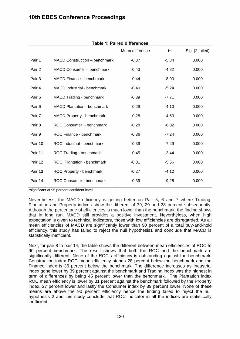
10th EBES Conference Proceedings
420
Table 1: Paired differences Mean difference t* Sig. (2 tailed)
Pair 1
MACD Construction – benchmark
-0.37
-5.34
0.000
Pair 2 MACD Consumer – benchmark
-0.43 -4.82 0.000
Pair 3 MACD Finance - benchmark
-0.44 -8.00 0.000
Pair 4 MACD Industrial - benchmark
-0.40 -5.24 0.000
Pair 5 MACD Trading - benchmark
-0.39 -7.71 0.000
Pair 6 MACD Plantation - benchmark
-0.29 -4.10 0.000
Pair 7 MACD Property - benchmark
-0.28 -4.50 0.000
Pair 8 ROC Consumer - benchmark
-0.28 -6.02 0.000
Pair 9 ROC Finance - benchmark
-0.36 -7.24 0.000
Pair 10 ROC Industrial - benchmark
-0.39 -7.49 0.000
Pair 11 ROC Trading - benchmark
-0.45 -3.44 0.000
Pair 12 ROC Plantation - benchmark
-0.31 -5.56 0.000
Pair 13 ROC Property - benchmark
-0.27 -4.12 0.000
Pair 14 ROC Consumer - benchmark
-0.39 -9.28 0.000
*significant at 95 percent confident level
Nevertheless, the MACD efficiency is getting better on Pair 5, 6 and 7 where Trading, Plantation and Property indices show the different of 39, 29 and 28 percent subsequently. Although the percentage of efficiencies is much lower than the benchmark, the finding shows that in long run, MACD still provides a positive investment. Nevertheless, when high expectation is given to technical indicators, those with low efficiencies are disregarded. As all mean efficiencies of MACD are significantly lower than 90 percent of a total buy-and-hold efficiency, this study has failed to reject the null hypothesis1 and conclude that MACD is statistically inefficient. Next, for pair 8 to pair 14, the table shows the different between mean efficiencies of ROC to 90 percent benchmark. The result shows that both the ROC and the benchmark are significantly different. None of the ROC’s efficiency is outstanding against the benchmark. Construction index ROC mean efficiency stands 28 percent below the benchmark and the Finance index is 36 percent below the benchmark. The difference increases as Industrial index gone lower by 39 percent against the benchmark and Trading index was the highest in term of differences by being 45 percent lower than the benchmark. The Plantation index ROC mean efficiency is lower by 31 percent against the benchmark followed by the Property index, 27 percent lower and lastly the Consumer index by 39 percent lower. None of these means are above the 90 percent efficiency hence the finding failed to reject the null hypothesis 2 and this study conclude that ROC indicator in all the indices are statistically inefficient.
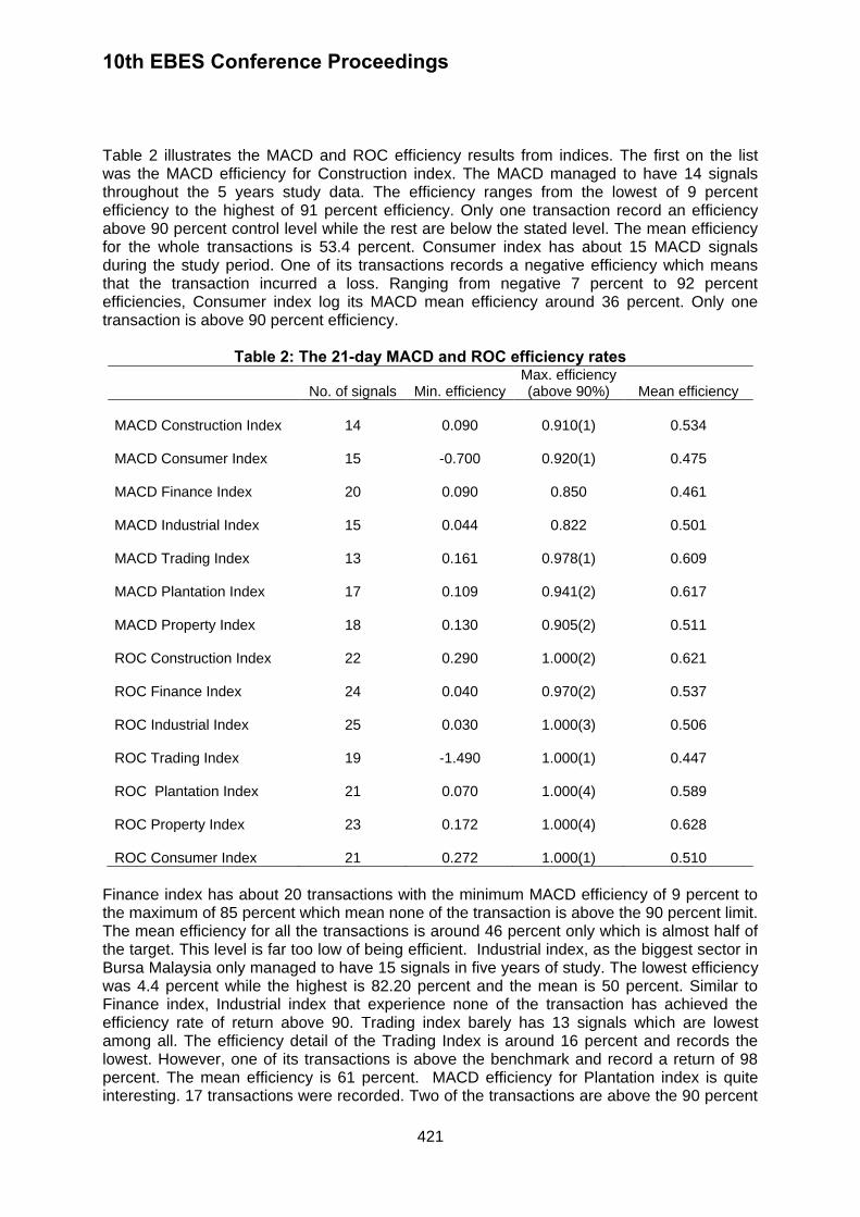
10th EBES Conference Proceedings
421
Table 2 illustrates the MACD and ROC efficiency results from indices. The first on the list was the MACD efficiency for Construction index. The MACD managed to have 14 signals throughout the 5 years study data. The efficiency ranges from the lowest of 9 percent efficiency to the highest of 91 percent efficiency. Only one transaction record an efficiency above 90 percent control level while the rest are below the stated level. The mean efficiency for the whole transactions is 53.4 percent. Consumer index has about 15 MACD signals during the study period. One of its transactions records a negative efficiency which means that the transaction incurred a loss. Ranging from negative 7 percent to 92 percent efficiencies, Consumer index log its MACD mean efficiency around 36 percent. Only one transaction is above 90 percent efficiency.
Table 2: The 21-day MACD and ROC efficiency rates
No. of signals Min. efficiency Max. efficiency (above 90%) Mean efficiency
MACD Construction Index 14 0.090 0.910(1) 0.534 MACD Consumer Index 15 -0.700 0.920(1) 0.475 MACD Finance Index 20 0.090 0.850 0.461 MACD Industrial Index 15 0.044 0.822 0.501 MACD Trading Index 13 0.161 0.978(1) 0.609 MACD Plantation Index 17 0.109 0.941(2) 0.617 MACD Property Index 18 0.130 0.905(2) 0.511 ROC Construction Index 22 0.290 1.000(2) 0.621 ROC Finance Index 24 0.040 0.970(2) 0.537 ROC Industrial Index 25 0.030 1.000(3) 0.506 ROC Trading Index 19 -1.490 1.000(1) 0.447 ROC Plantation Index 21 0.070 1.000(4) 0.589 ROC Property Index 23 0.172 1.000(4) 0.628 ROC Consumer Index 21 0.272 1.000(1) 0.510
Finance index has about 20 transactions with the minimum MACD efficiency of 9 percent to the maximum of 85 percent which mean none of the transaction is above the 90 percent limit. The mean efficiency for all the transactions is around 46 percent only which is almost half of the target. This level is far too low of being efficient. Industrial index, as the biggest sector in Bursa Malaysia only managed to have 15 signals in five years of study. The lowest efficiency was 4.4 percent while the highest is 82.20 percent and the mean is 50 percent. Similar to Finance index, Industrial index that experience none of the transaction has achieved the efficiency rate of return above 90. Trading index barely has 13 signals which are lowest among all. The efficiency detail of the Trading Index is around 16 percent and records the lowest. However, one of its transactions is above the benchmark and record a return of 98 percent. The mean efficiency is 61 percent. MACD efficiency for Plantation index is quite interesting. 17 transactions were recorded. Two of the transactions are above the 90 percent
10th EBES Conference Proceedings
422
benchmark with the highest of 94 percent and the lowest score of 11 percent. With mean efficiency around 62 percent, MACD for Plantation index may be promiseable. Lastly, the Property index, produces 18 signals altogether. The MACD efficiencies range from 13 percent to 91 percent with two of the transactions are above the 90 percent limit. The mean efficiency is only 51 percent. The second objective of the study seeks for the reliability of MACD in providing a good timing to enter and exit from the market. Table 1 exhibits that MACD efficiencies for all indices are significantly lower than the 90 percent level. Table two on the other hand, shows some MACD transactions outperformed the 90 percent level. However, these cases are remote. Having mean efficiencies from 46 percent to 62 percent, MACD may consider far too low to be efficient hence its reliability, to provide a good timing in investment, is questionable. Table 2 also discussed the efficiency of ROC. The first ROC efficiency was for Construction index. There are 22 signals of ROC for the whole 5 years data. The lowest efficiency is 29 percent with two transactions record an efficiency of 100 percent of the maximum buy-and-hold efficiency. The average efficiency for all the 22 transaction is 62 percent. ROC efficiency for Finance index documented about 24 transactions and lies between 4 percent and 97 percent, while two transactions out beat the 90 percent level. The mean efficiency is around 54 percent. Industrial index ROC efficiency managed to log in 25 numbers of transactions, and the highest among all. The efficiency levels varying from 3 to 100 percent. Three of its transactions are above 90 percent efficiency. ROC efficiency on Trading index managed to map down 19 transactions with one transaction recorded a negative 149 percent efficiency. That is a loss transaction for this particular investment. It also has a positive 100 percent efficiency in one of its transaction and the mean efficiency for the whole transactions is 45 percent. ROC efficiency on Plantation index draws 21 buy and sells transactions throughout the five years study and the efficiencies fall within 7 and 100 percent. Interestingly, four of its transaction managed to beat the 90 percent benchmark. The average efficiency is 59 percent. ROC of Property index registered 23 selected signals with efficiencies fall within 17 percent to100 percent. Four of its transactions outperformed the 90 percent level and the mean efficiency is 63 percent. This finding would interest some of the technical analyst in giving a consideration on ROC when analyzing the property sector. Lastly, the Consumer index confirmed 21 transactions within the selected years. The lowest efficiency is 27 percent which literally good and the highest efficiency is 100 percent which is excellent. Only one transaction goes beyond 90 percent level and the mean is 51 percent. This study suggested that ROC in Consumer index in general and Consumer sector related shares in particular would secure a good positive return in long run. 4. CONCLUSION Technical analysis has become essential to modern investment methodology and decision (Menkhoff, 1997). It offers more than hundred types of analysis to be employed in order to make the best decision of investment. The main idea of these analyses is to draw a maximum return at the minimum percentage of risks. To realize the goal, the technical indicators have to be efficient. This study found that all results failed to reject the null hypotheses and suggested that the traditional 21-day MACD and ROC as a whole are inefficient and failed to provide an analysis that secure a maximum return to the investor. New technical analysis, design and idea been introduced to meet the new challenge in investment market. Dynamic type of investment portfolios, policies and regulations and new technologies in news dissemination make technical analysis extremely important. Even though technical analysis has gone through transformations as new algorithms have replaced the old one but several traditional indicators remain relevant and applicable in
10th EBES Conference Proceedings
423
current market transaction including MACD and ROC. A study of MACD and ROC on individual share is recommended for a clear picture of its potential. This study looks at the macro level which provides some idea to investors and fund managers to switch between portfolio sectors when needed. REFERENCES Andrada, F.J. and Fernandez, R.F., 2008. Improving moving average trading rules with boosting and statistical learning method. Journal of Forecasting, 27(5), pp.433-449. Bauer, R.J. and Dahlquist, J.R., 1999. Technical market indicators: Analysis and performance. Canada: John Wiley & Sons, Inc. Caginalp, G. and Balenovich, D., 2003. A theoretical foundation for technical analysis. Journal of Technical Analysis, 59, pp.5-22. Dunis, C.L. and Chen, Y.X., 2005. Alternative volatility models for risk management and trading: An application to the EUR/USD and USD/JPY rates. Derivative Use, Trading and Regulation, 11(2), pp.125-156. Dunis, C.L., Laws, J., and Evans, B., 2006. Trading futures spreads: An application of correlation and threshold filters. Applied Financial Economics, 16(12), pp.903-914. Dzikevicius, A., Saranda, S. and Kravcionok, A. ,2010. The accuracy of simple trading rules in stock market. Economic and Management, 15, pp.910-916. Fong, W.M. and Yong, L.H.M., 2005. Chasing trends, recursive moving average trading rules and internet stocks. Journal of Empirical Finance, 12(1), pp.43-76. Garcia, M.E.F., Marin, E.A.d.l.C. and Garcia, R.Q., 2010. Improving return using risk-return adjustment and incremental training in technical trading rules with GAPs. Applied Intelligence, 33(2), pp.93-106. Gunasekarage, A. and Power, D. M., 2001. The profitability of moving average trading rules in South Asian stock markets. Emerging Markets Review, 2(1), pp.17-33. Kaufman, P.J., 2003. A short course in Technical Trading. Hoboken: New Jersey: John Wiley & Sons. Kung, J.J. and Wong, W.K., 2009. Profitability of technical analysis in the Singapore stock market, before and after the Asian financial crisis. Journal of Economic Integration, 24(1), pp.135-150. Marshall, B.R., Young, M.R., and Rose, L.C., 2007. Market timing with candlestick technical analysis. The Journal of Financial Transformation, 20(1), pp.18-25. Marshall, B.R., Cahan, R.H., and Cahan, J.M., 2008. Does intraday technical analysis in the U.S equity market have value? Journal of Empirical Finance, 15(2), pp.199-210. Menkhoff, L., 1997. Examining the use of technical currency analysis. International Journal of Finance and Economics, 2(4), pp.307-318.

10th EBES Conference Proceedings
424
Ming-Ming, L. and Siok-Hwa, L., 2006. The profitability of the simple moving averages and trading range breakout in the Asian stock markets. Journal of Asian Economics, 17(1), pp.144-170. Prings, M.J., 2001. Introduction to technical analysis. 1st Ed, Singapore: McGraw-Hill. Reilly, F.K. and Brown, K.C., 2003. Investment analysis and portfolio management. 7th Ed, South Western: Thomson. Sehgal, S. and Gupta, M., 2007. Tests of technical analysis in India. The Journal of Business Perspective, 11(3), pp.11-23.

PROCEEDINGS OF THE 10th EURASIA BUSINESS AND ECONOMICS SOCIETY CONFERENCE (EBES) - ISTANBUL
ISBN: 978-605-64002-1-6