10_simulation on maximum power point

ISSN 2278 – 8875

International Journal of Advanced Research in Electrical, Electronics and Instrumentation Engineering Vol. 1, Issue 3, September 2012

Copyright to IJAREEIE www.ijareeie.com 190

Simulation on Maximum Power Point

Tracking of the Photovoltaic Module using

LabVIEW

Dr. J. Abdul Jaleel, Nazar. A, Omega A R

Dept. of Electrical and electronics Engineering, TKM College of Engineering, Kollam, Kerala, India.

Abstract: Model of a solar cell and solar module is built in the LabVIEW software. Solar cell model is in single diode model

and it is solved by familiar Newton Raphson method. IV characteristics and PV characteristics are simulated in LabVIEW

and it verified at different temperature and irradiance conditions. Maximum power point tracking is incorporated in the

simulation of PV module and the Maximum power point, voltage and current at this maximum power point were simulated

at standard conditions and verified the result. The simulation system used for the analysis of solar photovoltaic module at

different temperature value, solar irradiation value, series resistance Rs and shunt resistance Rsh . Behavior of the solar

module in different diode ideality factor also analyzed. This model can be used for analysis of PV characteristics and for

simulation with Maximum Power Point Tracking Algorithm(MPPT) algorithms.

Key words: PVcell, PV module ,Maximum power point tracking, LabVIEW,Newton Raphson Method.

I. INTRODUCTION

Energy is required for the large number of thing from home to cars to electronics. The traditional energy used for these purpose are

coal natural gas, nuclear energy ,oil etc. Due to the crisis of traditional energy sources we need to find out the other source of

energy. Solar energy is a good option and the electricity produced is clean and silent. They are long lasting and having little

maintenance due to the absence of any moving part. The major disadvantages is their limited efficiency levels ;compared to other

renewable energy sources. The output of solar cell is greatly depend on the weather conditions and fluctuating in nature. So we

need to capture the maximum power from the solar panel. DC-DC converter based maximum power point tracking [2]is used for

this purpose .For the study of this kind we need the model of a solar cell or module to check the performance of MPPT going to

implement. Not only the MPPT system but also the device going to connect to the PV system need the model of a solar cell and the

panel and it is important in designing the storage batteries stand alone PV system, grid connected system etc. LabVIEW

(Laboratory Virtual Instrumentation Engineering Workbench ) is a good simulation as well as automation software , therefore the

PV cell and module model in LabVIEW is very important. This paper is organized as follow: Section I gives the introduction of

PV technology and the importance of mathematical simulation model in LabVIEW. Section II is helpful to understand the model of

solar cell and related equations in developing the simulation on LabVIEW. In section III model of solar module is designed with

the help of solar cell mathematical model and the section IV give Newton Raphson method for solving the nonlinear current

voltage equation. Section VI show the simulated result of solar module and at last section VII concludes the paper and followed by

the references.

II. MODEL OF A SOLAR CELL

Photovoltaic cell consist of PN junction that when exposed to light releases electrons. The solar cell can be modeled as a current

source parallel with a forward biased diode. The diode current Id is varies with the junction voltage Vd and the cell reverse

saturation current Io. Most popular method of modeling solar cell is the single diode model that is shown in Fig.1[5]-[9] . In

practical , solar cell is not ideal diode so there is some losses .In real cells, the effect is degraded by the presence of series resistance

Rs and parallel resistance Rsh . Series resistance Rs is very small, which arises from the ohmic contact between metal and

semiconductor internal resistance. But Shunt resistance Rsh is very large and represents the surface quality along the periphery.

Leakage of current through the periphery represents Ish. Both the diode current Id and shunt current Ish given by the photocurrent

Iph. In ideal case Rs is 0 and Rsh is ∞. The resultant current relationships are in the following equation, as dictated by Kirchhoff’s

Current Law [1]

IshIdIphI ………………………….........(1)

http://www.ijareeie.com/

ISSN 2278 – 8875



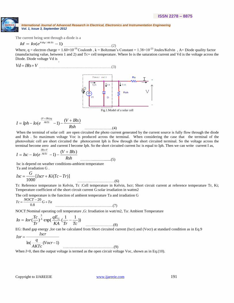
The current being sent through a diode is a

)1( / AkTcVdqeIoId……………………..…………(2)

Where, q = electron charge = 1.60×10-19

Coulomb , k = Boltzman’s Constant = 1.38×10-23

Joules/Kelvin , A= Diode quality factor

(manufacturing value, between 1 and 2) and Tc= cell temperature. Where Io is the saturation current and Vd is the voltage across the

Diode. Diode voltage Vd is ,

VIRsVd …………………………………………………(3)

Fig.1.Model of a solar cell

Rsh

IRsVeIoIphI AkTc

qIRsV)(

)1(

)(

………………….(4)

When the terminal of solar cell are open circuited the photo current generated by the current source is fully flow through the diode

and Rsh . So maximum voltage Voc is produced across the terminal. When considering the case that the terminal of the

photovoltaic cell are short circuited the photocurrent Iph is flow through the short circuited terminal. So the voltage across the

terminal become zero and current I become Iph. So the short circuited current Isc is equal to Iph. Then we can write current I as,

Rsh

IRsVeIoIscI AkTc

VIRs)(

)1(

………....................(5)

Isc is depend on weather conditions-ambient temperature

Ta and irradiation G .

)]([1000

TrTcKiIscrG

Isc ………..……………….(6)

Tr: Reference temperature in Kelvin, Tc :Cell temperature in Kelvin, Iscr; Short circuit current at reference temperature Tr, Ki;

Temperature coefficient of the short circuit current G:solar irradiation in wattm2

The cell temperature is the function of ambient temperature Ta and irradiation G

TaGNOCT

Tc

8.0

20

………………………………………(7)

NOCT:Nominal operating cell temperature ,G: Irradiation in watt/m2, Ta: Ambient Temperature

))11

(exp()(

3

TcTrKA

qE

Tr

TcIorIo GA

………………….(8)

EG: Band gap energy ,Ior can be calculated from Short circuited current (Iscr) and (Vocr) at standard condition as in Eq.9

)1(ln(

VocrAKTc

q

IscrIor

………………………………….(9)

When I=0, then the output voltage is termed as the open circuit voltage Voc, shown as in Eq.(10).


ISSN 2278 – 8875



0)1)exp(( Rsh

Voc

AKTc

qVocIoIsc …………………(10)

Then we can calculate the open circuit voltage ,Voc as

))(1ln(q

AKTc

Io

IscVoc

………………………………..(11)

III. MODEL OF A SOLAR MODULE

A PV array is a group of several PV cells which are electrically connected in series and parallel circuits to generate the required

current and voltage. The equivalent circuit for the solar module arranged in NP parallel and NS series cells.[6] is shown in Fig.2. If

the cells are connected in parallel, then the total voltage of all cells is the same as that of one cell but the total current is the sum of

the current values of the single cells. Since the current of a single cell can amount to more than 3 amp. and the voltage is less than

0.7 Volts, the parallel connection is rarely applied.

Fig.2.Equilent circuit of solar module

. The terminal equation for the current and voltage of the array becomes as follows

RshT

Ns

V

AKTc

IRsTNs

Vq

NpIoNpIscRshT

RsTI

)(

)1]

)(

(exp[)1(

..............(12)

Where

Total shunt Resistance ;

Rsh

Ns

NpRshT

Total series Resistance:

Rs

Np

NsRsT

IV. NEWTON RAPHSON ALGORITHM

Newton Raphson method is used for finding the root of a non linear function by successively better approximation[5]. If f(x) is a

non linear function the first step is to find the derivative f’(x). Next step ischoose an initial x value xn.Each successive value of x

closer to the value of x for f(x)=0,can be calculated by Eq.13

Here we take the value current instead of x.Then the Eq.(13) become

)('

)(1

n

n

nnIf

IfII

…………………………………………………….(13)

Then function of current can be expressed as


ISSN 2278 – 8875



RshT

Ns

V

AKTc

IRsTNs

Vq

NpIoNpIscRshT

RsTIIf

)(

)1]

)(

(exp[))(1()(

... (14)

The derivative of f,(I) is equal to

])

)(

(exp[)(1()('AKTc

IRsTNs

Vq

IoAKTc

qRsTNp

RshT

RsTIf

… (15)

When V=0 ,I=Isc .So we can start with the initial value I=Isc .

V. RESULTS

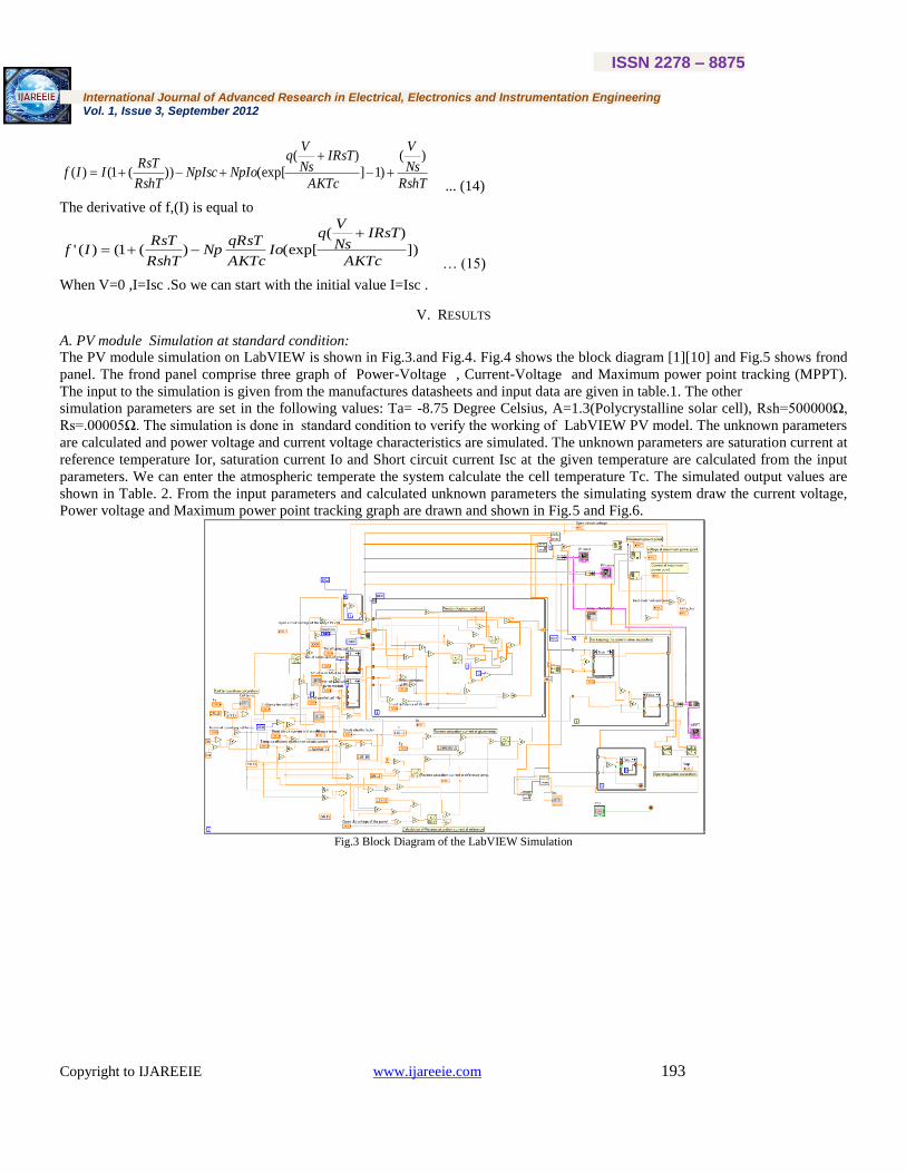
A. PV module Simulation at standard condition: The PV module simulation on LabVIEW is shown in Fig.3.and Fig.4. Fig.4 shows the block diagram [1][10] and Fig.5 shows frond

panel. The frond panel comprise three graph of Power-Voltage , Current-Voltage and Maximum power point tracking (MPPT).

The input to the simulation is given from the manufactures datasheets and input data are given in table.1. The other

simulation parameters are set in the following values: Ta= -8.75 Degree Celsius, A=1.3(Polycrystalline solar cell), Rsh=500000Ω,

Rs=.00005Ω. The simulation is done in standard condition to verify the working of LabVIEW PV model. The unknown parameters

are calculated and power voltage and current voltage characteristics are simulated. The unknown parameters are saturation current at

reference temperature Ior, saturation current Io and Short circuit current Isc at the given temperature are calculated from the input

parameters. We can enter the atmospheric temperate the system calculate the cell temperature Tc. The simulated output values are

shown in Table. 2. From the input parameters and calculated unknown parameters the simulating system draw the current voltage,

Power voltage and Maximum power point tracking graph are drawn and shown in Fig.5 and Fig.6.

Fig.3 Block Diagram of the LabVIEW Simulation


ISSN 2278 – 8875



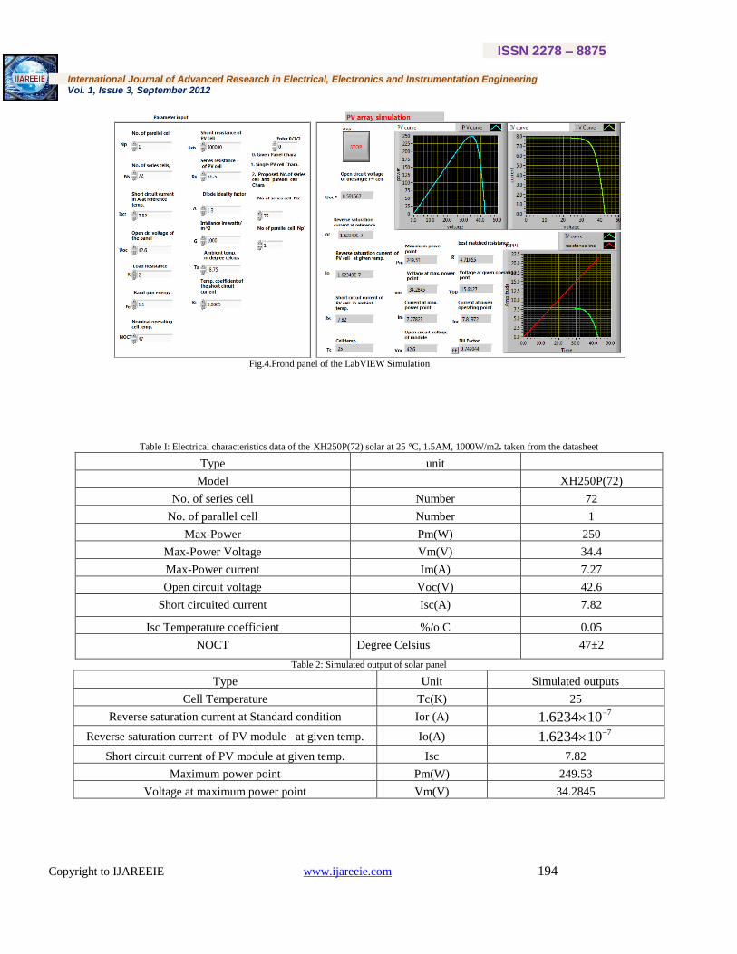
Fig.4.Frond panel of the LabVIEW Simulation

Table I: Electrical characteristics data of the XH250P(72) solar at 25 °C, 1.5AM, 1000W/m2. taken from the datasheet

Type unit

Model XH250P(72)

No. of series cell Number 72

No. of parallel cell Number 1

Max-Power Pm(W) 250

Max-Power Voltage Vm(V) 34.4

Max-Power current Im(A) 7.27

Open circuit voltage Voc(V) 42.6

Short circuited current Isc(A) 7.82

Isc Temperature coefficient %/o C 0.05

NOCT Degree Celsius 47±2

Table 2: Simulated output of solar panel

Type Unit Simulated outputs

Cell Temperature Tc(K) 25

Reverse saturation current at Standard condition Ior (A) 7106234.1 Reverse saturation current of PV module at given temp. Io(A)

7106234.1 Short circuit current of PV module at given temp. Isc 7.82

Maximum power point Pm(W) 249.53

Voltage at maximum power point Vm(V) 34.2845


ISSN 2278 – 8875



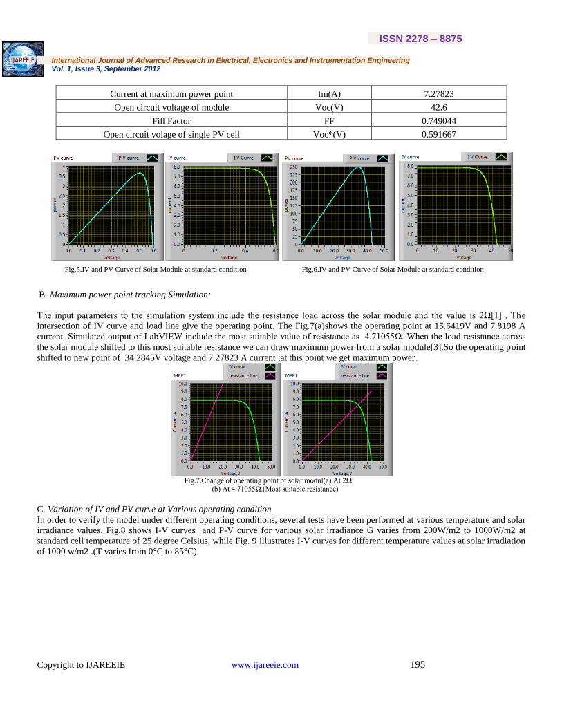
Current at maximum power point Im(A) 7.27823

Open circuit voltage of module Voc(V) 42.6

Fill Factor FF 0.749044

Open circuit volage of single PV cell Voc*(V) 0.591667

Fig.5.IV and PV Curve of Solar Module at standard condition Fig.6.IV and PV Curve of Solar Module at standard condition

B. Maximum power point tracking Simulation:

The input parameters to the simulation system include the resistance load across the solar module and the value is 2Ω[1] . The

intersection of IV curve and load line give the operating point. The Fig.7(a)shows the operating point at 15.6419V and 7.8198 A

current. Simulated output of LabVIEW include the most suitable value of resistance as 4.71055Ω. When the load resistance across

the solar module shifted to this most suitable resistance we can draw maximum power from a solar module[3].So the operating point

shifted to new point of 34.2845V voltage and 7.27823 A current ;at this point we get maximum power.

Fig.7.Change of operating point of solar modul(a).At 2Ω (b) At 4.71055Ω.(Most suitable resistance)

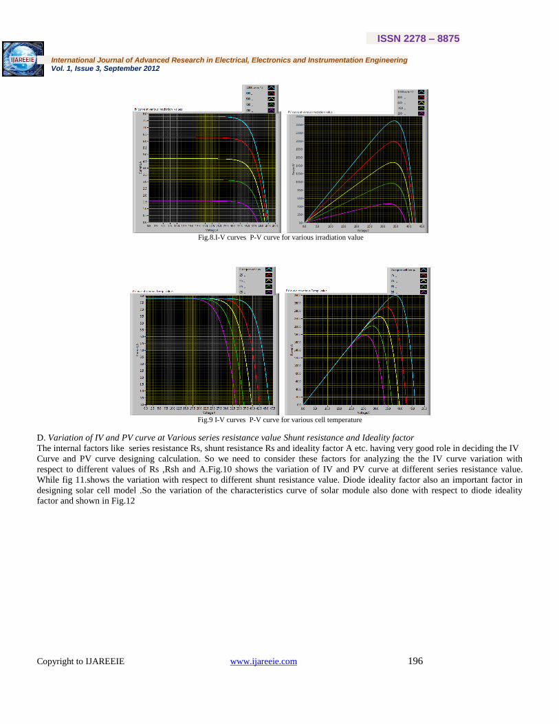
C. Variation of IV and PV curve at Various operating condition

In order to verify the model under different operating conditions, several tests have been performed at various temperature and solar

irradiance values. Fig.8 shows I-V curves and P-V curve for various solar irradiance G varies from 200W/m2 to 1000W/m2 at

standard cell temperature of 25 degree Celsius, while Fig. 9 illustrates I-V curves for different temperature values at solar irradiation

of 1000 w/m2 .(T varies from 0°C to 85°C)


ISSN 2278 – 8875



Fig.8.I-V curves P-V curve for various irradiation value

Fig.9 I-V curves P-V curve for various cell temperature

D. Variation of IV and PV curve at Various series resistance value Shunt resistance and Ideality factor

The internal factors like series resistance Rs, shunt resistance Rs and ideality factor A etc. having very good role in deciding the IV

Curve and PV curve designing calculation. So we need to consider these factors for analyzing the the IV curve variation with

respect to different values of Rs ,Rsh and A.Fig.10 shows the variation of IV and PV curve at different series resistance value.

While fig 11.shows the variation with respect to different shunt resistance value. Diode ideality factor also an important factor in

designing solar cell model .So the variation of the characteristics curve of solar module also done with respect to diode ideality

factor and shown in Fig.12


ISSN 2278 – 8875



Fig.10 IV curves and P-V curve for various series resistance value

Fig.11.I-V curves P-V curve for various Shunt resistance value

Fig.12.I-V curves P-V curve for various Diode ideality factor value


ISSN 2278 – 8875



VI. CONCLUSIONS

In this work, it is found that the current voltage relationship is non linear and there is a maximum power at a particular current and

voltage .This maximum power is varying with respect to the atmospheric condition such as irradiation value of solar light

,atmospheric temperature and wind speed etc. In this analysis the of effect irradiation and atmospheric temperature on current -

voltage characteristics and power- voltage characteristics are studied . When the irradiation level reduced the photo generated

current reduced significantly. The open circuit voltage (Voc) is reduces also reduced but the effect is negligible. In decreasing

atmospheric temperature value, at solar irradiation of 1000 w/m2 ,open circuit voltage is only decreased and the photo generated

current remain constant . In effect the power is decreases with increase in temperature. When analyzing the effect of series

resistance, we can see that the Isc and Voc remain constant but the maximum power point is varying. The series resistance

influences the slope of the IV characteristics at the constant voltage region. At the same time parallel resistance Rsh influences the

slope of the curve at the constant current region. The fill factor is affected by the change in parallel and series resistance. Ideality

factor have a role in finding the maximum power point of solar cell at given condition. Ideality factor (A) having value between 1

and 2 and we can see that power peak of a PV Curve is affected by the ideality factor of the solar cell. This model can be used for

analysis of PV characteristics and for simulation with MPPT algorithms.

ACKNOWLEDGEMENTS

The authors would like to thank the management, and Faculty Members, of Department of Electrical and Electronics Engineering,

TKM College of Engineering, Kollam, for many insightful discussions and the facilities extended to us for completing the task.

REFERENCES

[1] M., YANG Gang, CHEN Ming “LabVIEW Based Simulation System for the Output Characteristics of PV Cells and the Influence of Internal Resistance on It,” WASEInternational Conference on Information Engineering ,Vol.1,pp.391-394,2009

[2] Joung-Hu Park, Jun-Youn Ahn, Bo-Hyung Cho and Gwon-Jong Yu” DualModule-Based Maximum Power Point Tracking Control of Photovoltaic System

,” IEEE Trans., Vol. 53,no.4, pp .1036-1047,.2009. [3] Johan H. R. Enslin, Mario S. Wolf, Dani¨el B. Snyman, and Wernher Swiegers, “Integrated Photovoltaic Maximum Power Point Tracking Converter,” IEEE

Trans., Vol. 44,no.6, pp. 1036-1047, Aug .2009.

[4] R.Ramaprabha ,Badrilal Mathur K.Santhosh,S.Sathyanarayanan ”Modeling and Simulation of SPVA Characterization under all Conditions,” In International Journal of Emerging Trends in Engineering and Technology , Vol.1.No.1, 2011.

[5] Patel, H.; Agarwal, V. “MATLAB-Based Modeling to Study the Effects of Partial Shading on PV Array Characteristics” IEEE Trans.Energy

conversion,Vol.23,No.1,2pp.302-310,2008. [6] L.Nguyen, “Modeling and Simulation of Solar PV Arrays under Changing Illumination Conditions,” In Proc. IEEE Workshops on Computer in Power

Electronics, ,pp. 866-870, 16-19 July 2005.

[7] Swiegers, “W. An integrated maximum power point tracker for photovoltaic panels” In Proc. ISIE '98, 7-10 july 1998,vol.1,pp.41-44 [8] Sonal Panwar and Dr. R.P. Saini , “Development and Simulation of Solar Photovoltaic model using Matlab/simulink and its parameter extraction” In Proc.

International Conference on Computing and Control Engineering (ICCCE 2012),12-13 april 2012.

[9] Hannes HoKnopf“ Analysis and Evaluation of Maximum power point tracking(MPPT)Method for a solar powered vehicle,” M. Eng. thesis, Portland state university, 1999.

[10] Joseph Durago, “Photovoltaic Emulator adaptable to irradiance, Temperature and panel specific IV curve”, M. Eng. thesis, California Polytechnic State

University, San Luis Obispo,june 2011.

Authors Biography

1Abdul Jaleel. J received the Bachelor degree in Electrical Engineering from University of Kerala, India in

1994. He received the M.Tech degree in Energetics from Regional Engineering College Calicut, Kerala, India in

2002, and PhD from WIU, USA in 2006.

He joined the EEE department of TKM College of Engineering as faculty member in 1990. He was with Saudi

Aramco in 1996 to 1998 and worked in the field of power generation, transmission, distribution and

instrumentation in the Oil and Gas sector of Saudi Arabia. He was with Water Supply department of Sultanate of Oman in 1985 to

1986 and worked with the maintenance of Submersible bore-well pumps and power supplies. He was with Saudi Electricity

Company in 1979 to 1985 and worked in the Generation, Transmission and distribution fields. He worked with project management,


http://ieeexplore.ieee.org/xpl/articleDetails.jsp?tp=&arnumber=4453994&contentType=Journals+%26+Magazines&refinements%3D4291944246%26queryText%3DModel+of+photovoltaic+cell+circuits+under+partial+shading

http://ieeexplore.ieee.org/search/searchresult.jsp?searchWithin=p_Authors:.QT.Swiegers,%20W..QT.&newsearch=partialPref

ISSN 2278 – 8875



Quality Management and he is a certified Value Engineer and Auditor for QMS. He is a consultant for Oztern_Microsoft,

Technopark, Kerala and Consultant for Educational Projects of KISAT and MARK Research and Education Foundation.

Currently he is a P.G. Coordinator of M. Tech Programme in the TKM College of Engineering under University of Kerala and

Director of Kerala Institute of Science and Technology. His main areas of research are power system optimization, power system

reliability, voltage stability, computer aided design and analysis.

Omega A R

She received B.Tech Degree in Electrical and Electronics Engineering from Thangal Kunju Musaliar College of Engineering, Kollam, India.

Currently she is pursuing M.Tech in Industrial Instrumentation and Control at the same college.


10_simulation on maximum power point

Documents