1040 no. estimating 3-d egomotion perspective … and conference papers...1040 ieee transactions on...

1040 IEEE TRANSACTIONS ON PAlTERN ANALYSIS AND MACHINE INTELLIGENCE, VOL. 12, NO. 11, NOVEMBER 1990

Estimating 3-D Egomotion from Perspective Image Sequences

Wilhelm Burger and Bir Bhanu, Senior Member, ZEEE

Abstract- This paper deals with the computation of sensor motion from sets of displacement vectors obtained from consecutive pairs of images. The problem is investigated with emphasis on its application to autonomous robots and land vehicles. First, the effects of 3-D camera rotation and translation upon the observed image are discussed and in particular the concept of the focus of expansion (FOE). It is shown that locating the FOE precisely is difficult when displacement vectors are corrupted by noise and errors. A more robust performance can be achieved by computing a 2-D region of possible FOE-locations (termed the fuzzy FOE) instead of looking for a single-point FOE. The shape of this FOE-region is an explicit indicator for the accuracy of the result. It has been shown elsewhere that given the fuzzy FOE, a number of powerful inferences about the 3-D scene structure and motion become possible. This paper concentrates on the aspects of computing the fuzzy FOE and shows the performance of a particular algorithm on real motion sequences taken from a moving autonomous land vehicle.

Zndex Tenns-Autonomous mobile robot, dynamic scene analysis, fuzzy focus of expansion, motion analysis, passive navigation, sensor motion estimation.

I. INTRODUCTION HE problem of determining the motion parameters of a T moving camera relative to its environment from a sequence

of images is important for the application of computer vision in mobile robots. Short-term control, such as steering and braking, path stabilization, navigation, and obstacle avoidance are all tasks that can effectively utilize this information [ l l ] , [12]. Several researchers have addressed this problem directly [3], [lo], [17], [19] or indirectly by determining the motion parameters of a single rigid object with respect to a stationary camera [9], [14], [21], [28], [30]. Since the (stationary) environment can be considered as one large rigid object, these two approaches are equivalent. A prerequisite for any existing method is to estimate the 2-D motion that occurs in the image between consecutive frames. Two basic methods have been proposed for this purpose, which are quite distinct.

The gradient method [20], [29] uses spatial and temporal gray- level variations to estimate the instantaneous velocity or optical flow at each location in the image. It relies on sufficient object texture, continuous motion, and small displacements between subsequent frames. Since the magnitude of flow can only be determined in the direction of 2-D gradient, i.e., perpendicular to the tangent of a boundary, the flow vectors cannot be computed locally. This is commonly referred to as the aperture problem [31]. Global smoothing of the flow field has been proposed,

Manuscript received August 20, 1987; revised May 16, 1990. Recom- mended for acceptance by W. B. Thompson. This work was supported by the Defense Advanced Research Projects Agency under Contract DACA 76-86- C-0017 and monitored by the U.S. Army Engineer Topographic Laboratories.

W. Burger was with Honeywell Systems and Research Center, 3660 Technology Drive, Minneapolis, MN 55418. He is now with the Institute of Systems Science, Johannes Kepler University, Linz, Austria.

B. Bhanu is with Honeywell Systems and Research Center, 3660 Technol- ogy Drive, Minneapolis, MN 55418.

IEEE Log Number 9038388.

which gives rise to problems at flow discontinuities, such as object boundaries. This seems to be almost a paradox, since intuitively motion estimates should be obtained most easily at exactly those locations.

The displacement method [2], [4] uses the parts of the image where discontinuities in brightness or motion occur (which are a source of problems in the gradient method). Significant features such as line segments, distinct dark or bright spots, or comers in two consecutive frames are selected and matched, rendering a field of displacement vectors for those features. This results in a formulation of 2-D motion as discrete displacements as compared to the velocity-based formulation which characterizes the gradient method. Ideally, the selected features should not only be matched between subsequent frames, but tracked over multiple frame sequences. Two problems arise during this process. The first problem is the selection and reliable location of significant features in consecutive frames, especially when the images are noisy. Individual features are commonly extracted by applying local window operations, like Moravec’s “interest operator” [23] as a classic example. The application of this approach on a mobile land-based robot faces additional difficulties. In this particular scenario, a forward-looking camera moves approximately parallel and at relatively small distance to the ground. Therefore, visual objects in the environment “approach” the camera from almost infinite distance to as close as a few meters, before they leave the field of view. A point which was clearly distinguishable when observed from some distance, may lose its sharp outlines when the camera gets closer to it. This suggests some form of range- dependent feature-extraction from the image [ 181. The second problem is finding reliable matches between the set of interesting points extracted from one frame and the set of interesting points extracted from the subsequent frame. This has been termed the correspondence problem [4] which is, although a nontrivial task in itself, assumed to be solved in the context of this work.

In spite of the persisting difficulties, the displacement method appears to be more promising than the gradient method. Not only is the information contained in discrete displacements fields of more practical use, but the problem of reliably computing optical flow is as hard as extracting and matching distinct features and has theoretical limitations [32]. In this work, we use a discrete feature matching approach, a local technique, where significant (i.e., “interesting” [23]) image events are localized in both images and subsequently matched upon similarity [4], [18]. This results in a field of displacement vectors between corresponding feature points.

From a given set of image displacement vectors, the 3-D structure of the scene and its relative motion towards the camera can be obtained simultaneously by solving a system of linear or nonlinear equations [ 141, [21], [28], [30]. While this technique is known to be numerically unstable under noisy conditions, recent work [15], [33] demonstrates that improvements are possible or that error estimates can be obtained.

0162-8828/90/110~1040$01.00 0 1990 IEEE

BURGER AND BHANU: ESTIMATING 3-D EGOMOTION 1041

When the camera is looking forward and the platform motion is characterized by a significant translation component (which is typical for most vehicles), another technique becomes attractive. It relies upon the fact that, under pure camera translation, all image features seem to diverge from a particular image location, called the focus of expansion (FOE), which marks the direction of vehicle heading [8], [20], [22], [24], [26]. This is of course only true for the stationary part of the scene but moving objects may be handled individually [l]. The advantage of this method is that the FOE, and consequently all parameters of the egomotion, can be computed entirely in terms of 2-D image coordinates regardless of the spatial structure of the scene.

We have adopted the FOE method as the basis of our approach. Unfortunately, computation of a single location for the FOE turns out to be a hard problem, mainly due to digitization errors, unreliable displacement vectors, and image noise. There seems to be psychological evidence 1271 that humans also have difficulties in estimating the precise direction of heading in comparable situations. Our solution to the problem is not to search for a single FOE-location, but to obtain a two-dimensional FOE- region, which we call the “fuzzy F O E [13]. Despite the apparent loss in accuracy, the Fuzzy FOE can be employed as a practical tool in dynamic scene analysis [6] , [12]. In the following sections, we discuss the effects of camera motion upon the image and ways to decompose these effects. We distinguish between the FOE-from-rotation and rotation-from-FOE approaches, whiqh are characterized by opposite search strategies in the multi- dimensional parameter space. Although the latter approach turns out to be superior, the actual location of the FOE can generally not be determined precisely under noisy conditions. A description of the fuzzy FOE algorithm is followed by some typical results on real image sequences which were taken from the autonomous land vehicle (ALV).

11. IMAGE EFFECTS OF 3-D CAMERA MOTION It is well-known that any rigid motion of an object in space

between two points in time can be decomposed into a combi- nation of translation and rotation. While many researchers have used a velocity-based formulation of the problem [l], [26], the following treatment views motion in discrete time steps. Given the world coordinate system shown in Fig. 1, a translation T = (U V W)’ applied to a 3-D point X = (X Y Z)‘ is accomplished through vector addition: X’ = T + X .

A 3-D rotation R about an arbitrary axis through the origin of the coordinate system can be described by successive rotations R+, Re, and R, about its X-, Y-, and Z-axes, respectively. Thus, X ’ = R X = R,+R,R,X, where

0 cos0 0 sin0

-sin0 0 cos6

(1)

cos$ sin$

The transformation M for arbitrary rigid motion in three-space is thus given by

Fig. 1. Camera model showing the coordinate system, lens center, image plane, and angles of rotation. The origin of the coordinate system 0 is located at the lens center. The focal length f is the distance between the lens center and the image plane.

rotation matrices is not commutative, a different order of rotations would result in different amounts of rotation for each axis. For a fixed order of application, however, this motion decomposition is unique.

To model the environment of the vehicle, the camera is considered as being stationary and the environment as being moving as one single rigid object relative to the camera. The origin of the coordinate system (Fig. 1) is located in the lens center of the camera. The given task is to reconstruct the vehicle’s egomotion from visual information. It is therefore necessary to know the effects of different kinds of vehicle motion upon the observed image.

Under perspective imaging, a point X = (X Y Z)’ in 3-D space is projected onto a location in the image plane x = (x y)’, with

where f is the focal length of the camera (see Fig. 1).

A. Effects of Pure Camera Rotation

The effects caused by pure camera rotation about an axis passing through the lens center are intuitively clear (see Fig. 1). For example, if the camera is rotated about the Z-axis (i.e., the optical axis), points in the image move along circles centered at the image location n, = (0 0). In practice, however, we can assume that the amount of rotation about the Z-axis is relatively small and we therefore, only consider the more significant rotations about the X- and Y-axes.

Rotating the vehicle about the X-axis by an angle -4 and about the Y-axis by an angle -0 moves each 3-D point X to a new location X’, given as

X + X ’ = R + . R , . X

0 sin 0 X

Consequently x, the image point of X, moves to x‘ given by,

M : X + X ’ = R+&R+(T+ X ) ,

with six degrees of freedom (4,0, $, U, V, and W ) . This decomposition is not unique because the translation could be applied after the rotation instead. Also, since the multiplication of the

X c o s 0 + Z s i n 0

I042 IEEE TRANSACTIONS ON PATTERN P

Inverting the perspective transformation from (3) and using it in (4) leads to the 2-D rotation mapping ?-,To which moves each image point x = (zy) into the corresponding image point x' = (x'y') under the sequence of 3-D rotations R,Ro,

R , R s ( X ) : x + X '

T , T ~ ( z ) : z = (x y) + 2' = (2' y')

[ i:] f --2 cos 4 sin 0 + y sin 4 + f cos 4 cos 0

' [zs in4s inB + y c o s 4 - f s i n 4 c o s o 1 - (6)

It is important to notice that this transformation contains no 3-D variables, such that its effects can be simulated without knowing the distance of the observed points from the image plane. Therefore, the acquired image changes when the camera rotates around its lens center, but no additional, entirely new views of the environment are obtained. Ignoring the effects at the boundary of the image and errors due to the discretization of the image, we can assume that pure camera rotations merely map the image to itself.

To compute the amount of rotations from a pair of observations, we need to solve the inverse problem. Given are two image locations xo and xI, which are the projections of a 3-D point X at time to and time t l , what are the amount of rotation 4 and B which when applied to the camera between instances to and t I , would move image point xo onto xI, assuming that no camera translation has occurred?

If horizontal rotation R, and vertical rotation RO are applied to the camera separately, the points in the image move along hyperbolic paths [24]. If pure rotation Rs were applied to the camera, a given image point 2,) = (xuy,,) would move on a path described by

:c cos 0 + f sin B

Similarly, pure vertical rotation R, would move an image point x1 = (xclyl) along a path described by

Since the composite 3-D rotation is modeled as two separate steps (RQ followed by Rd), the rotation mapping, T,TQ, can also be separated into T~ followed by T, . In the first step T ~ ,

rotation around the Y-axis, moves the original image point xo to an intermediate location x,. Subsequently, T , would take point x, to the final location x, by camera rotation around the X-axis. All this can be expressed as

where

and

T , : Z c = (ZcYc) + 2 1 = (21 Y l ) . (8)

As shown in Fig. 2, the image point x, = (zcyc) is located at the intersection of a horizontal hyperbola passing through xo (7a)

iNALYSIS AND MACHINE INTELLIGENCE, VOL. 12. NO. 1 1 . NOVEMBER 1990

Fig. 2. Effects of camera rotation. Rotation about the Y-axis is applied first, which moves the arbitrary image point xo along a hyperbolic path to xc. Subsequent rotation downwards about the X-axis moves x, to x1 . The image location x( is found by intersecting the two hyperbolae passing through xo and X I .

and a vertical hyperbola through xI (7b). The coordinates of the intersection point x, are

From this, the angles of rotation B and 4 (for this particular order of rotations) are finally obtained as (see Fig. 2),

-tan-' E! (10) 0 = tan-' c. -tan-' 3 4 = tan-' f f ' f f '

B . Effects of Pure Camera Translation

When the vehicle undergoes pure translation T = (U V W)' between time to and t l , every point X , in the environment moves relative to the vehicle by the vector -T. Since every stationary point is affected by the same translation vector, these points actually move along imaginary parallel lines in 3-D space. It is a fundamental result from perspective geometry [16] that the images of parallel lines pass through a single point in the image plane called a vanishirig point (Fig. 3). Therefore, when the camera moves forward along a straight line in space, image points seem to diverge from this vanishing point (the focus of expansion-FOE) or converge towards it (the focus of contraction-FOC) when the camera moves backwards.

Fig. 3 demonstrates that the straight line passing through the lens center 0 of the camera and the FOE is also parallel to the 3-D motion _vectors of the environmental points. Therefore, the 3D vector OF (from lens center to FOE) points in the direction of camera translation in space but does not supply the length of T . The actual translatiy vector T applied to the camera is a multiple of the vector OF:

T = A 0 3 = X[X, yf f ] ' , X E R. (1 1)

In velocity-based models of 3-D motion, the FOE has fre- quently been interpreted as the direction of instantaneous heading, i.e., the direction of vehicle translation during an infinitely short period of time. When images are given as a sequence of snapshots taken at discrete instances of time with significant image motion in between, a discrete model seems more appro- priate that treats the FOE as the direction of accumulated vehicle translation over a certain period of time.

BURGER A N D BHANU: ESTIMATING 3-D EGOMOTION 1043

Fig. 3. Effects of camera translation in the forward direction. Under pure camera translation, points in the environment (A,B,C) move relative to the camera along parallel 3-D vectors in space. These parallels have a common vanishing point x, = ( . r f yf) (the focus of expansion, FOE), in the perspective image, from which all displacement vectors seem to expand.

1) Measuring the Amount of Camera Translation: Fig. 4 shows the geometric relationships for measuring the amount of camera translation for the 2-D case. It can be considered as a top view of the camera, i.e., a projection onto the X/Z-plane of the camera-centered coordinate system. The cross section of the image plane is shown as a straight line. The camera is translating from left to right in the direction given by T = (xf f)T. A stationary 3-D point is observed at two instances of time, which moves in space relative to the camera from X to X’, resulting in two images x and x’.

X = [:] and X ‘ = [::I = [,-,,]. X - A X

Using the inverse perspective transformation from (3) yields

Z = -X and Z‘ = 2 - A 2 = -X’ = -(X - AX). f f f 5 2’ 2

From similar triangles (shaded in Fig. 4)

AX AZ -- - - “f f ’

and therefore

Thus, the rate of expansion of image points from the FOE contains direct information about the distance of the corresponding 3-D points from the camera. Consequently, if the vehicle is moving along a straight line and the FOE has been located, the 3-D structure of the scene can be determined from the expansion pattern in the image. However, the distance Z of a 3-D point from the camera can only be obtained up to the scale factor AZ, which is the distance that the vehicle advanced along the Z-axis during the elapsed time.

When the velocity of the vehicle (AZ/t) in space is known, the absolute range of any stationary point can be computed. Altematively, the linear velocity of the vehicle can be obtained if the actual range of a point in the scene is known (e.g., from laser range data), In practice, of course, any such technique requires that the FOE can be located in a small area, and that the observed

Fig. 4. Amount of expansion from the FOE for discrete time steps. The camera moves by a vector T in 3-D space, which passes through the lens center and the FOE in the image plane. The 3-D Z-axis is also the optical axis of the camera.

image points exhibit significant expansion away from the FOE. As will be shown in the following section, image noise and camera distortion pose serious problems in the attempt to assure that both of the above criteria are met.

If a set of stationary 3-D points {(XtXi)} is observed, then of course the translation in the Z-direction is the same for every point.

Therefore, the range of every point is proportional to the observed amount of expansion of its image away from the FOE,

x: -xf 2, o( - x: - 2, ’

which renders the relative 3-D structure of the set of points. The effects of camera translation T can be formulated as a

mapping t between two ordered sets of corresponding image points I = {z,} and I‘ = {s:}. Unlike in the case of pure camera rotation, this mapping not only depends upon the 3-D translation vector but also upon the position of each point in 3-D space. Therefore, the quantitative image effects of a particular translation T cannot be predicted without knowing the actual 3-D structure of the scene. However, there is an important qualitative property of the 2-D mapping t, namely that each point maps onto a straight line passing through the original point and the FOE, i.e., if the vehicle undergoes pure forward translation, then there must exist one image location xf , such that t is a radial mapping between Z and I‘ with respect to x,. In other words, the condition

radial-mapping (I, I’ , zf ) : t = {(2*,2:) E I x I’ I 2: = 2, + p,(s, - s,),

P, E R, L 0) must be satisfied. This observation is the key for decomposing the effects of arbitrary camera motion into its translational and rotational components.

111. DECOMPOSITION OF IMAGE MOTION The image effects of a composite 3-D camera motion M :

X + X’ = R+Re(T + X) can be summarized by a mapping d : In + I , = rmrst(In), where d stands for displacement and

1044 IEEE TRANSACTIONS ON PATTERN ANALYSIS AND MACHINE INTELLIGENCE, VOL. 12, NO. 1 I , NOVEMBER 1990

the mapping transforms the original image Io into the subsequent image I , . For the purpose of clarity, we introduce the intermediate image I' = t I o which is the result of the translation component of the vehicle's motion such that the condition radial-mapping (Io, I*, xf) is satisfied for some xP Unlike the two images Io and I , , this new image I* is generally not observed, except when no camera rotation occurs. It serves as an intermediate result to be reached during the separation of the translational and rotational motion components.

Fig. 5 shows the top view of a vehicle traveling along a curved path to explain this decomposition. At the two instances in time to and t , , the position of the vehicle in space is specified by the location of a reference point (i.e., the lens center) P and the orientation R of the vehicle with respect to its environment. The original image Io is seen at time to. Following the adopted scheme of motion decomposition, the translation T is applied first, which takes the vehicle's reference point from position Po to position PI without changing its orientation Ro. This transforms image Io into image I* . Notice that the FOE is found at the intersection of the 3-D translation vector T with the image plane Io. In the second step, the vehicle is rotated by w to its new orientation R I , generating the final image II.

To allow a unique reconstruction of the actual motion parameters R,, Rs, Rc., and T from their 2-D effects, a minimum number of environmental points must be included in the computation. Tsai and Huang [30] have shown that seven points in two perspective views suffice to obtain a unique interpretation in terms of rigid motion and structure, except for a few cases where points are arranged in some very special configuration in space. Ullman [3 11 reports computer experiments which indicate that six points are sufficient in many cases and seven or eight points yield unique interpretations in most practical cases. Of course, to reduce the effects of noise and tracking errors, in practice we will always try to include some redundancy by observing a much larger set of environmental points.

The fact that

t I" = I' = ?-;lT-;'Il (13)

suggests two altemative strategies for separating the motion components.

1 ) FOE from Rotation: Successively apply combinations of inverse rotational mappings (?-;'TG,'), ( T ~ ~ T ; ~ ' ) , . . . , (TG'T;;)

to the second image I , , until the resulting image I' is a radial mapping with respect to the original image Io. Then locate the FOE zfk in Io.

2 ) Rotation from FOE: Successively select FOE-locations zf,, zf2, . . . , zfr, (different directions of vehicle translation) in the original image Io and see if inverse rotational mappings (?<'?;%') exist that yield a radial mapping with respect to the selected FOE zf7, in the original image Io .

Both altematives were investigated under the assumption of realistic forward vehicle motion. Although originally the first approach had appeared more attractive, it tumed out to be difficult to determine how close a given displacement field is to being radial when the location of the FOE is not given. In the presence of noise, this problem becomes even more difficult. The second approach was examined after it appeared that any method which extends the given set of displacement vectors backwards to find the FOE is inherently sensitive to image degradations [6].

In practice, the displacement vectors may not pass through a single pixel. Even for human observers it seems to be difficult to determine the exact direction of heading (i.e., the location of the FOE on the retina). Average deviation of human judgement from

Fig. 5. Interpretation of the focus of expansion (FOE) for discrete time steps. Vehicle motion between its initial position (where image Z0 is observed) and its final position (image I , ) is modeled as two separate steps. (a) First the vehicle translates by a 3-D vector T from position PO to position P I without changing its orientation 610. After this step, the intermediate image I* would be seen. Subsequently (b), the vehicle rotates by changing its orientation from Ro to R I . Now image ZI is observed. The FOE is found where the vector T intersects the image plane IO (and also I*) .

the real direction has been reported to be as large as 10" and up to 20" in the presence of large rotations [25]. It was, therefore, an important premise in this work that the final algorithm should determine an area of potential FOE-locations (called the fuzzy FOE) instead of a single (but probably incorrect) point. In the following, we briefly describe the FOE from rotation method and then present the details of our rotation from FOE technique.

A . FOE from Rotation

In this method, the image motion is decomposed in two steps. First, the camera rotations are estimated and their inverse effects are applied to the second image I , , thus producing a "derotated" image I f . If the rotation estimate was accurate, the resulting displacement field from Io to I ' should be radial since only the effects of camera translation remain. The second step verifies that the displacement field is actually radial and determines the location of the FOE. In the FOE from rotation approach, two problems have to be solved:

1) How to estimate the rotational motion components without knowing the exact location of the FOE?

2) How to measure the "goodness of derotation" and locate the FOE?

There are several ways to get an initial estimate for the rotations. If the platform has sufficient inertia, the results from one pair of frames can be carried over to the following pair as an initial guess. Also, the displacement vectors of points at far distance from the camera (known from earlier observations) are not significantly affected by translation and can be used to obtain an immediate estimate for the rotations [e.g., using (lo)]. Another approach is discussed by Bhanu and Burger [51, t61, where the range of possible rotations is successively constrained by geometric operations.

After applying the inverse rotations to the second image I , , the question is how much the resulting displacement field between Io and the derotated image I' deviates from a radial mapping. Of course, due to finite image resolution, noise, and inaccuracies from point tracking, we can never expect any mapping to be perfectly radial. Prazdny [24] suggests to measure the disturbance of the displacement field by computing the variance of the intersections of one displacement vector with all other vectors. If those intersections lie close together, then the variance is small,


indicating that the displacement field is almost radial. Similarly, instead of selecting a particular displacement vector, one could compute the intersection with imaginary horizontal or vertical lines, as was pursued by Bhanu and Burger [5 ] , [61.

Common to this class of techniques is that they all need to extend the given displacement vectors backwards along straight lines to find their intersections which, of course, multiplies the disturbances caused by m y existing errors. This is particularly true for short displacement vectors. As a consequence, the error functions to measure the quantitative deviation from a radial displacement field are not well-behaved under noisy conditions. They usually exhibit local minima which prohibit efficient search for the optimal derotation (see Bhanu and Burger [5], [6] for details).

B . Rotation from FOE While the above method iterates over rotation angles, the

rotation from FOE technique, discussed in the following, successively evaluates potential FOE-locations. An initial guess for the FOE may be obtained from knowledge about the orientation of the camera relative to the vehicle. Subsequently, the solution from the previous frame pair can be used as a starting point. Once a particular FOE, xf , has been selected, the problem is to find the rotational mappings T;' and T;' which, when applied to the image Z, to produce Z', will result in an optimal radial mapping between Zo and I' with respect to a given FOE, xf. To apply a local search strategy (e.g., the method of steepest descent), we need a suitable error function that is well behaved in a large region around the global minimum.

The error measure that was chosen for this purpose uses the deviation of the displacement vectors from straight rays originating from the selected FOE. Given a set of corresponding image points {(x,~:) E I o x 1') and some FOE-location xf the error measure E is defined as

Fig. 6 shows the interpretation of this error measure as the sum of the squared perpendicular distances of the displacement vectors' end points from the radial lines. Notice that this expression implicitly puts more weight upon the long (i.e., dominant) displacement vectors and less on short ones.

Since under perspective transformation, image points move along hyperbolic paths when the camera performs pure rotation, the resulting displacement is not uniform over the entire image plane (7). However, if the amount of rotation is small (less than 4") or the focal length of the camera is large, we can replace the nonlinear mappings ~ 8 ' and T;' by a linear shift vector S+g which is independent of the image location, i.e.,

I* = r;lT.;lIl M S@ + I1 = I + . (15)

Notice that this assumption does not imply that the algorithm is valid just for small rotations. It only serves as an approximation to estimate the optimal rotation angles more quickly. In most practical cases, this condition is satisfied, provided that the time interval between frames is sufficiently small. However, should the amount of vehicle rotation be very large for some reason, a coarse estimate of the actual rotation can

I

Fig. 6. Measuring the deviation from a radial displacement field. For the assumed FOE-location xf, d,'s are the perpendicular distances between the endpoints of the displacement vectors and radial lines emanating from xf and passing through xi's. The sum of the squared distances is used to quantify the deviation from a radial displacement field with respect to xf.

be found and applied to the image before the FOE computation [6]. With sO0 as a free variable, the error measure (14) becomes

where x, E I and x', E I' . This second-order error function can be minimized with stan-

dard numerical techniques to obtain an optimal value for ~ $ 0 . To reduce this problem to a one-dimensional search, one point xR, called the guiding point, is selected in image Zn which is forced to maintain zero error for its displacement vector. Therefore, the corresponding point must lie on a straight line passing through x: and xf. Any shift s (see Fig. 7) applied to the set of image points 2' E I' must keep x: on this straight line, i.e., x: = xk + s = zCf + X(x, - x ~ f ) for all s, and thus,

s = xf - X; + X(Z, - xf), X E R. (17)

For example, for X = 1, s = x9 - x; which is the negative of the displacement vector from xg to xi. In this case, xi and zg would overlap.

This leaves X as the only free variable and the error function ( 16) becomes

E(X) = [AA, - B, + C,I2 (18) 2

with

1

Differentiating (18) with respect to X and setting the result equal to zero yields the parameter Xwt for the optimal shift sop, as

CA,B, - cA,C, c A? Xopt =

1046 IEEE TRANSACTIONS ON PAITERN ANALYSlS AND MACHINE INTELLIGENCE, VOL. 12, NO. 1 1 , NOVEMBER 1990

Fig. 7. Use of a guiding point. The problem is to register the two images I = { s, } and I' = { .r: } onto a radial pattem out of the FOE xf (dashed lines) by shifting the second image I' uniformly by some (unknown) 2-D vector s. We simplify this to a 1-D search by selecting a displacement vector x, .+ xh whose deviation from the radial line must be zero under any shift vector s. Intuitively, this means that the entire image I' is first shifted such that xk coincides with a radial line through xn ( 1 ) and then I' is translated parallel to this line (2) until a minimum error is reached.

The optimal shift vector sopt is obtained using (17). However, to evaluate the selected FOE-location xf, we are primarily interested in the error value E(Xop,) that would result from applying the approximate derotation sopt. E(Xop,) is obtained by inserting A,, into (18), giving

or

The normalized error EN shown in the results that follow (Figs. 9-15) is defined as

where N is the number of displacement vectors used for computing the FOE.

Since in a displacement field caused by pure camera translation all vectors must point away from the FOE, this restriction must hold for any candidate FOE-location (Fig. 8). If after applying soP(xf) to the second image Z ' , the resulting displacement field contains vectors pointing toward the hypothesized xf , then this FOE-location is prohibited and can be discarded from further consideration. Fig. 8 shows a field of five displacement vectors. The optimal shift sopc for the given xf is shown as a vector in the lower right-hand comer. When sop[ is applied to point zi, the resulting displacement vector (shown with a heavy line) does not point away from the FOE. Since its projection onto the line

points toward the FOE, it is certainly not consistent with a radial expansion pattem.

The following function Evaluate-SingleFOE examines one hypothetical FOE-location xr in a given pair of images Io and I , . It uses the functions Optimal-Sh$t for computing the optimal shift vector sop and Equivalent-Rotation to obtain the rotation

..@'?!- ,'FOE

A:; Fig. 8. FOE-locations are prohibited if the displacement field resulting from the application of the optimal shift sop, contains vectors pointing towards the FOE. This is the case at point XI.

angles equivalent to sOpt [by (IO)]. The parameters and Omax are the maximum angles of rotation for which the approximation in (15) is acceptable. If the estimated rotation angles exceed that limit, the intermediate image Z+ is derotated exactly by procedure Derotate-Zmage [using (6)] before another estimate is computed.

Evaluute_Single_FOE(xf, Io , Z I , &,,ax, Omax): I+ t I , ; (4,@ +- (0,O);

repeat /* usually only one iteration required */ (sOpt, error) t Optimal-Shijt(Zo, I+ , xf); (@, 0+) +- Equivalent-Rotation (soPC); (4,O) + (40) + ( 6 9 e+); I++- Derotute-Image ( I , , 4,O); until (6 5 &ax & B+ 5 Om,,)

retum (I+, $,d , error).

The error function E is computed in time proportional to the number of displacement vectors N . The final size of the FOE- area depends on the local shape of the error function and can be constrained not to exceed a certain maximum M . Therefore, the time complexity is O ( M N ) .

The first set of experiments was conducted on synthetic imagery to investigate the behavior of the error measure under various conditions, namely

the average length of the displacement vectors (longer displacement vectors lead to a more accurate estimate of the FOE), the amount of residual rotation components in the image, and the amount of noise applied to the location of image points.

Fig. 9 shows the distribution of the normalized error EN for a sparse and relatively short displacement field (length factor = 2 = 8 pixels) containing 7 vectors. Residual rotation components of +2" in horizontal and vertical direction are present in Fig. 9(b)-(d) to visualize their effects upon the image. The displacement vector through the guiding point is marked with a heavy line. The choice of this point is not critical, but it should be located at a considerable distance from the FOE to reduce the effects of noise upon the direction of the vector

In Fig. 9, the error function is sampled in a grid with a width of 10 pixels over an area of 200 by 200 pixels around the actual FOE, which is marked by a small square. The size of the circle at each location indicates the amount of error, i.e., the deviation from the radial displacement field that would result if that location were picked as the FOE. Heavy circles


o o o . . . . . . . . 0 0 0 0 0 o n o . . . . . . . . n n o o o 1 0 0 . . . . . .

d

length-faclor= 1 0 rotation- 0 0 O F d+g

lmaqe Plane

I I 0 0 D . . . . .... 0 0 0 0 0

d

Image Plane

\ \

?ngth-factor- 2 0 ?tatten- 2.0 0 0 deg

.

\

length-factor- 2 0 r"1.3110". O F - 2 0 dag

Fig. 9. Error function for a synthetic displacement field. Displacement field and minimum error at selected FOE-locations. The shape of the error function is plotted over an area of flOO pixels around the actual FOE (marked with a small square). The diameter of each circle reflects the amount of normalized error (21) for that particular FOE-location. Heavy circles indicate error values above a certain threshold (4.0), prohibited locations (as defined earlier) are marked "+". (a) No residual rotation. (b) 2.0" of horizontal camera rotation (camera rotated to the left). (c) 2.0' vertical rotation (camera rotated upwards). (d) -2.0' vertical rotation (camera rotated downwards).

indicate error values which are above a certain threshold (4.0). Those FOE-locations that would result in displacement vectors which point toward the FOE (as described earlier) are marked as prohibited (+). It can be seen that this two-dimensional error function is smooth and monotonic within a large area around the actual FOE (marked by a small square). The shape of this error function makes it possible that, even with a poor initial guess, the global optimum can be found by local search methods.

Figs. 10 to 15 show the effects of various conditions upon the behavior of this error function in the same 200 x 200 pixel square around the actual FOE as in Fig. 9.

An important criterion is the function's behavior when the amount of camera translation is small or the displacement vectors are noisy. Fig. 10 shows the effects of varying the average length of the displacement vectors in the range of 4-60 pixels in the absence of any residual rotation or noise

(except digitization noise). Note that longer displacement vectors result in a sharper minimum around the actual FOE.

Fig. 11 shows the effect of increasing residual rotation in horizontal direction upon the shape of the error function: Fig. 12 shows the effect of residual rotation in vertical direction. Here, it is important to notice that the displacement field used is extremely nonsymmetric along the Y-axis of the image plane. This is motivated by the fact that in real ALV images, long displacement vectors are most likely to be found from points on the ground, which are located in the lower portion of the image. Therefore, positive and negative vertical rotations have been applied in Fig. 12.

In Fig. 13, residual rotations in both horizontal and vertical direction are present. It can be seen [Fig. 13(a)-(e)] that the error function is quite robust against rotational components in the image. The result in Fig. 13(e) shows the effect of large combined rotation of 4.0°/4.00 in both directions. Here, the minimum of

1048 IEEE TRANSACTIONS ON PATTERN ANALYSIS A N D MACHINE INTELLIGENCE, VOL. 12, NO. 1 1 , NOVEMBER 1990

error < I O . error = I O error = 2.0 o ernr - 3.0 0 error I 4 0 0 error > 4 0 + prohibited

(a) (b) (c) ( 4 (e) length-factor- 1 0 length-faclor- 2.0 length-factor. 5 0 length-factor. 10 0 length-factor- 15.0 rolation. 0.0 0.0 deg rotation- 0.0 0.0 deg noire- +- 0.0 P X I S uniform noire. +- 0.0 pxlr uniform

rotation- 0.0 0.0 deg noire. +- 0.0 p x l ~ unilorm

rotation- 0.0 0 0 deg noise. +- 00 pxlr uniform

rotation. 0.0 0.0 deg noice- +- 0 0 pxls uniform

Fig. 10. Effects of increasing the average length of displacement vectors upon the shape of the error function. The same displacement field as in Fig. 9 was used. (a) Average length is 4 pixels, (b) 8 pixels, (c) 20 pixels, (d) 40 pixels, (e) 60 pixels. (Length factor varies from 1 to 15.) Note that FOE is better defined by longer displacement vectors.

error < 1 0 . error - 1.0 I) error - 2.0 o error = 3 0 0 error = 4 0 o error > 4.0 + prohihiled

(a) (b) (c) ( 4 (e) lenglh-laclor= 2.0 Ienglh-factor. 2.0 length-lactor- 2 0 length-laclor. 2.0 length-laclor- 2.0 rotation- 0.0 0 0 deg noise- +- 0 0 pxlr unitnrm

rotalion= 0.1 0.0 deg ncise- +- 00 pxlr unilorm

rotation- 0 5 0 0 deg noise- +- 0 0 pxlr uniform

rotations 1.0 0 0 deg n c i v = +- 0 0 pxls uniform

relation. 2.0 0 0 dog noiw= +- 0 0 pxlr unlfnrm

Fig. 11. Effects of increasing residual rotation in horizontal direction upon the shape of the error function for relatively short vectors (length factor 2.0). No noise was applied.

(b) (c) ( 4 (e) (a) length-factor- 2.0 length-factor- 2.0 length-factor- 2 0 length-factor. 2.0 length-faclor- 2.0 rolalion. 0 0 -2 0 &g nlire= +- 0 0 p x l ~ uniform

rotalion- 0.0 -1 0 deg noire- +- 0.0 pxls uniform

rotation; 0.0 0 0 deg nois?= +- 0.0 pxlr uniform

rotation- 0.0 1.0 deg noise- +- 0.0 pxlc uniform

rolation- 0.0 2 0 dsg noire. +- 0 0 XIS uniform

Fig. 12. Effects of increasing residual rotation in vertical direction upon the shape of the error function for relatively short vectors (length factor 2.0). No noise was applied.

the error function is considerably off the actual location of the FOE because of the error induced by using a linear shift to approximate the non-linear derotation mapping. In such a case, it would be necessary to actually derotate the displacement field by the amount of rotation equivalent to sOpt found at the minimum of this error function and repeat the process with the derotated displacement.

The effects of various amount of noise are shown in Fig. 14. For this purpose, a random amount (with uniform distribution) of displacement was added to the original (continuous) image location and then rounded to integer pixel coordinates. Random displacement was applied in ranges from f0.5 to k4.0 pixels in both horizontal and vertical direction. Since the displacement field contains only seven vectors, the results do not provide

BURGER A N D BHANU: ESTIMATING 3-D EGOMOTION 1049

Fig. 13.

Fig. 14.

* o n . . . . . . . . n o o n o 0 0 0 . 1 . . .... 0 0 0 0 0 c o o . . . . . . . " l ) O 0 0 0 . .

a * o , . , . . . . . . " O O * @ " 0 0 0 . . . . .... 0 0 0 0 0 . . . 0 0 000

. O O O @ O 0 " " 0 . . . . g * * * . . . . . .

(c) ( 4 ' (e) lenglh-faclor= 2 0 length-factor; 2.0 rotation; 2.0 2.0 deg noire- +- 0.0 XIS unlform

(a) (b) ienglh-factor= 2 0 length-factor; 2 0 length-factor= 2 F rotalion; 0.0 0 0 deg noise- + - 0 O F X ~ S uniform

rotation- 0.5 0.5 deg noise. +- 0 o pxis uniform

rotation- 1.0 1.0 deg noire. +- 0 0 pxis uniform

rotation- 4 .0 4.0 deg noise= +- 0.0 F X I ~ unifnrm

Effects of increasing residual rotation in horizontal and vertical direction upon the shape of the error function for relatively short vectors (length factor 2.0). No noise was applied.

(a) (b) (c) ( 4 (e) length-faclor. 50 length-factor- 5.0 length-faclor. 5 0 length-factor. 5.0 length-factor. 5.0 rotation- 0.0 0.0 deg noise- +- 0.0 pxlt uniform

rotation- 0.0 0 0 deg noise- +- 4 0 pxls uniform

rotalion. 0.0 0.0 deg noise- +- 0 5 pxlr uniform

rotation. 0.0 0.0 deg noise- +- 1 0 pxlr uniform

rotation- 0.0 0 0 dag noire. +- 2 0 p x l ~ uniform

Effects of varying the amount of noise. Uniform noise was applied to the same displacement field as in Fig. 9. (a) Zero noise, (b) 50.5 pixels, (c) k1.0 pixels, (d) k2.0 pixels, (e) k4.0 pixels. The error function becomes flat with increasing noise levels.

information about the statistical effects of image noise. This would require more extensive modeling and simulation. How- ever, this figure serves as an indicator for the amount of noise present in the image and the reliability of the final result. It can be observed that the error function flattens out with increasing levels of noise, although the generic shape of the function does not change. Further, the location of the global minimum error may be located considerably off the actual FOE which makes it difficult to locate the FOE precisely under noisy conditions.

Again, it should be noted that the length of the displacement vectors is an important factor. The shorter the displacement vectors are, the more difficult it is to locate the FOE correctly in the presence of noise. Fig. 15 shows the error functions for two displacement fields with different average vector lengths. For the shorter displacement field (length-fuctor 2.0) in Fig. 15(a), the shape of the error function changes dramatically [compare Fig. 13(a)]. A search for the minimum error would inevitably converge toward a point indicated by the small arrow, far off the actual FOE. For the image with length-factor 5.0 [Fig. 15(b)], the minimum of the error function coincides with the actual location of the FOE (a). The different result for the same constellation of points in Fig. 14(d) is caused by the different random numbers (noise) obtained in each experiment. This experiment shows that a sufficient amount of displacement between consecutive frames is essential for

reliably determining the FOE and thus, the direction of vehicle translation.

These experiments demonstrate the need to somehow quantify the reliability of the resulting FOE by analyzing the local shape of the error function. Our goal is therefore not to compute a single FOE, but rather a 2-D distribution of possible FOE-locations. The final result is a connected image region, which we call a "Fuzzy FOE," that can be assumed to contain the actual FOE with high certainty. The following algorithm describes the basic steps in computing the Fuzzy FOE for a given pair of images Zo and Z I :

F u z ~ y F O E ( l o , Z I ) :

1) Guess an initial FOE, XO.

2) Starting from xo, search for an FOE, x,,,, with minimum error (following the steepest descent).

3) Around x,,,, grow a connected region such that the error for each member FOE location is below a given limit.

In implementing this algorithm, several measures can be taken to improve its efficiency. First, the required search in steps 2) and 3 ) can be done over a grid of varying resolution from coarse to fine. To eliminate multiple evaluations of the same FOE-location (by function Evulua teS ing leFOE) , results could be kept for later reference, e.g., in a hash table. Finally, FOE-locations can be evaluated in parallel if suitable hardware is available. Results from computing the Fuzzy FOE on real data taken from a moving ALV are shown in the following section.

1050

I

IEEE TRANSACTIONS ON PATTERN ANALYSIS AND MACHINE INTELLIGENCE, VOL. 12, NO. 11, NOVEMBER 1990

I I 1 I

c

Image Plane

000000~0..... . . . . . O 0 0 0 0 * o o o . . . . . . . . . . . 0 0 0 0 U O O o 0 . . . . . . . . . . 0 0 OOOOooor..... . . . . . O D 0000000~...... ~ o ~ ~ o 0 0 0 . . . . . .I : : : ::: .. . . . . . . . .

I

I d ?nglh-factor. 2.0 >talion- 0.0 0.0 deg (a) &e- t- 20 pxlr unicorn

- J'

?nglh-laclor* 5.0 ,lation. 0.0 0.0 deg eke. t- 2.0 pxlr unirorm

IV. EXPERIMENTAL RFSULXS In the following, the results of the FOE-algorithm and compu-

tation of the vehicle's velocity over ground (see Appendix) are shown on a real image sequence, illustrated in Fig. 16, taken from the moving ALV. The spatial resolution in these images is 512 x 512 pixels. The vehicle traveled at approximately 14 kilometers per hour and the elapsed time between each pair of frames is 0.5 seconds, such that the translation vector has a length of about 1.9 meters.

For the experiment described in the following, points were tracked manually after computing binary edge images from the original sequence. Since some information (e.g., color cues) that is useful for a human observer is lost in the process of edge detection, the potential performance of an automatic tracking procedure should not be too far from these results. The assumption was that points that are significant in an edge image should also be relatively easy to track by a program, as compared to points which are subjectively selected in a high- quality color image. Recent experiments [7], [18], in fact, indicate that adequate results can be obtained by selecting and tracking point features in a fully automatic mode.

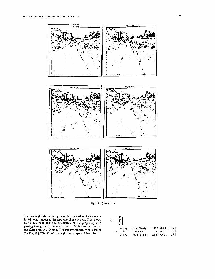
Approximately 25 points were selected in each image and the period of observation for these points was in the range of 2-16 frames. The particular types of local image features considered were endpoints and comers of lines as well as centers of small closed regions. Features on the road surface, which are important for estimating camera motion, turned out to be difficult to follow from frame to frame when they are approached by the vehicle. Since the edge operator uses the same mask regardless of the 3-D distance of the feature, the resulting edge image may change dramatically when features get closer and change their scale. A successful implementation for feature extraction and tracking will need to take this into account and employ some form of range-dependent image operation [7], [18]. Fig. 17 shows 16 edge images of the original ALV sequence (Fig. 16), where the selected feature points are labeled with numbers.

Fig. 18 shows the final results of computing the vehicle's motion for the sequence in Fig. 16. Each frame n at time t displays the motion estimates for the period between t and the previous frame n - 1 at time t - 1. Therefore,

the first motion estimate is available after the second frame (n = 183). Throughout, in search for the FOE, the optimal FOE-location (i.e., the one with minimum error) from the previous frame pair was taken as the initial guess. For the very first pair of frames, the FOE was guessed from the known camera orientation relative to the vehicle.

Each motion estimate consists of three components: a) the fuzzy FOE, b) the angles of horizontal and vertical rotation, and c) the approximate distance traveled over ground. The fuzzy FOE is marked by a shaded area of varying shape and size. The jagged outline of the fuzzy FOE is caused by the relatively coarse grid (10 pixels wide) used for growing the region. The small circle inside this region marks the location of the optimal FOE. The shape of the FOE-region depends strongly upon the most dominant (longest) displacement vectors in the scene. Since these vectors are usually found in the lower central parts of the image, the FOE tends to be elongated along the vertical axis, i.e., the horizontal position of the FOE is usually better defined than its vertical position. This may be different, of course, for other types of scenes.

The estimates for the rotations in horizontal and vertical direction are shown in a coordinate frame *lo in the lower left-hand comer of each image. Since the amount of rotation is relatively small, it was never necessary to apply intermediate derotation during the FOE search. Along with the original displacement vectors (solid lines), the vectors obtained after derotation (dotted lines) are also shown.

The absolute velocity of the vehicle is estimated after computing the FOE (see Appendix). The essential measure used for this calculation is the height of the camera above the ground, which is constant and known (3.3 meters). If the road is assumed to be flat and parallel to the direction of vehicle translation, the 3-D distances of points on the road surface and thus the amount of vehicle translation can be found in absolute terms. The estimated advancement (in meters) between each frame pair is also given in Fig. 18. Since points on the road, particularly those close to the camera, are difficult to track, these estimates are approximate.


Fig. 16. A sequence (frames 182-197) taken from a moving autonomous land vehicle (ALV). The Scene contains two moving objects, one car moving away from the ALV and another car approaching the ALV.

V. CONCLUSIONS The goal of this work was to develop a robust technique for

computing the parameters of self-motion of a land vehicle from visual information. This information is useful for a variety of tasks, such as vehicle control, navigation, obstacle avoidance, etc. It turned out that particularly the direction of heading (i.e., the focus of expansion-FOE) is difficult to compute under practical conditions, i.e., finite image resolution, noise, and feature tracking errors.

Our solution to this problem is not to search for a single-point FOE, but rather to determine a 2-D region of possible FOE-locations (termed the fuzzy FOE), whose shape is an explicit indicator for the reliability of the result. It is particularly suited for motion sequences that exhibit a significant translation component, i.e., for most vehicular applications. In contrast to other methods, however, the fuzzy FOE performs well even under the conditions of small rotation, image noise and also provides a measure for the quality of the result. Experiments show that even erroneous point matches in the given image displacement vector field can be tolerated, which is absolutely necessary in a fully automated process.

Although land-based vehicles and autonomous robots have been considered as the main application, the approach appears to be useful in other environments as well. For example, the described algorithm has been successfully applied to images taken from a helicopter flying at low altitude [7], where the rotations are much more significant than in the examples shown here.

APPENDIX

COMPUTING V E L O C ~ OVER GROUND In the following, it is shown how the absolute velocity of

the vehicle can be estimated after the location of the FOE has been determined. The essential measure used for this calculation is the absolute height of the camera above the ground which is constant and known. As discussed in Section 11, from the derotated displacement field and the location of the FOE, the 3-D layout of the scene can be obtained up to a common scale factor (12). This scale factor and, consequently, the velocity of the vehicle can be determined if the 3-D position of one point in space is known. Furthermore, it is easy to show [16] that it is sufficient to know only one coordinate value of a point in space to reconstruct its position in space from its location in the image. As the ALV travels on a fairly flat surface, the road can

be approximated as a plane which lies parallel to the vehicle’s direction of translation (see Fig. 19). This approximation holds at least for a good part of the road in the field of view of the camera. Since the absolute height of the camera above the ground is constant and known, it is possible to estimate the positions of points on the road surface with respect to the vehicle in absolute terms. From the changing distances between these points and the camera, the actual advancement and speed can be determined.

First, a new coordinate system is introduced which has its origin in the lens center of the camera. The Z-axis of the new system passes through the FOE in the image plane and points, therefore, in the direction of translation. The original camera-centered coordinate system (XYZ) is

1052 IEEE TRANSACTIONS ON PA'lTERN ANALYSIS AND MACHINE INTELLIGENCE, VOL. 12, NO. 11, NOVEMBER 1990

FRAME 182

FRAME 184

FRAME 186

FRAME 183

I

. - , ";: 1 .@' - . ! . ' "

\.

. . I__-

p , -. .

FRAME 185

FRAME 187

I

Fig. 17. ALV image sequence (frames 182-197) after edge detection and point selection. Points were tracked manually on these images from one frame to the next and labeled with numbers. The actual image location of each point lies at the lower left-hand comer of the corresponding label.

transformed into the new frame (X' Y'Z') merely by applying horizontal and vertical rotation until the Z-axis lines up with the FOE.

The horizontal and vertical orientation in terms of pan and tilt are obtained by "rotating" the FOE (x,y,) into the center of the image (00) using (10):

6, = -tan-' 7, 4f = -tan-'


I FRAME 190

A. . - -

FRAME 192

F Fig. 17. (Continued. )

The two angles 8, and 4, represent the orientation of the camera in 3-D with respect to the new coordinate system. This allows us to determine the 3-D orientation of the projecting rays passing through image points by use of the inverse perspective transformation. A 3-D point X in the environment whose image x = (xy ) is given, lies on a straight line in space defined by

cos 8, sin 8 sin 4, -sin 8, cos 4f

sin Of -cos 8, sin 4f cos 8, cos or cos 4f

1054 lEEE TRANSACIl0N.S ON PATIERN ANALYSIS AND MACHINE INTELLIGENCE, VOL. 12, NO. 11, NOVEMBER 1990

F R A M 194 FRAME 195

Fig. 17. (Continued)

FRAM 182 FRAME 183 I

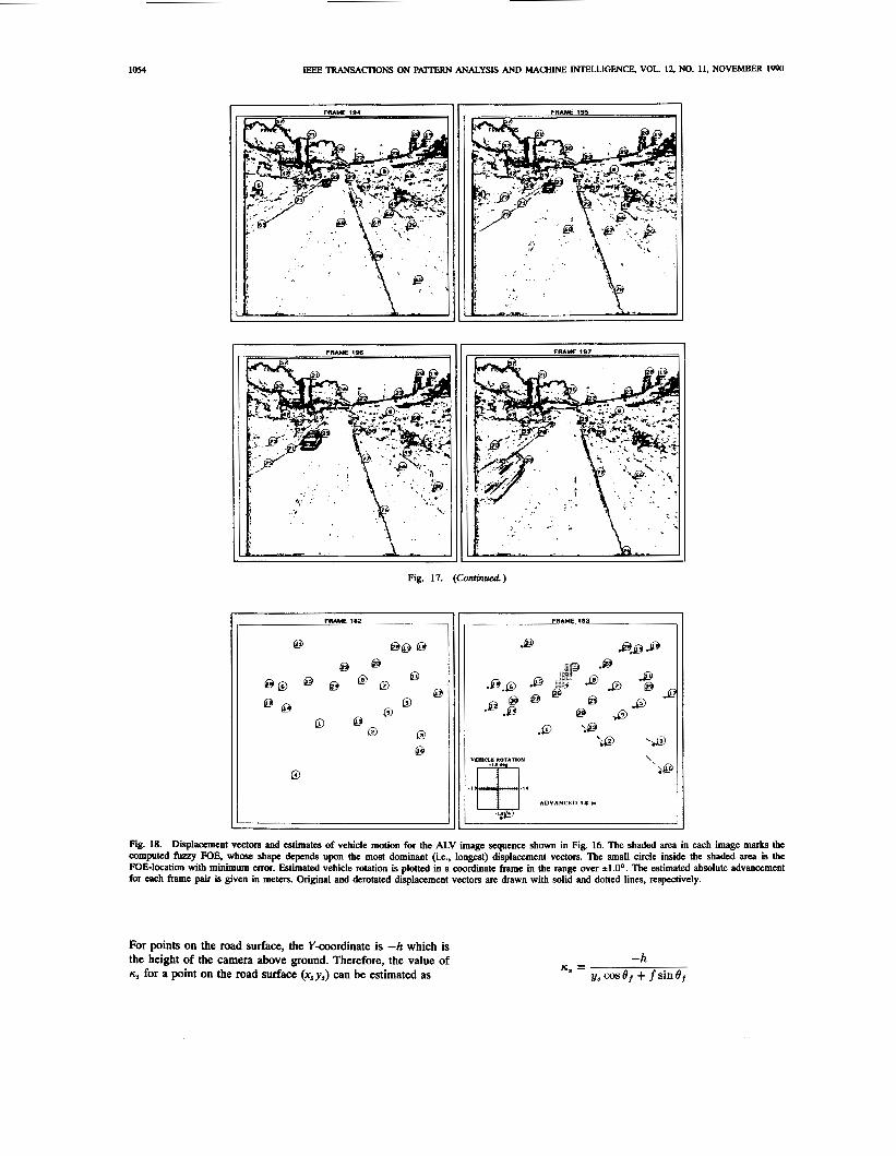
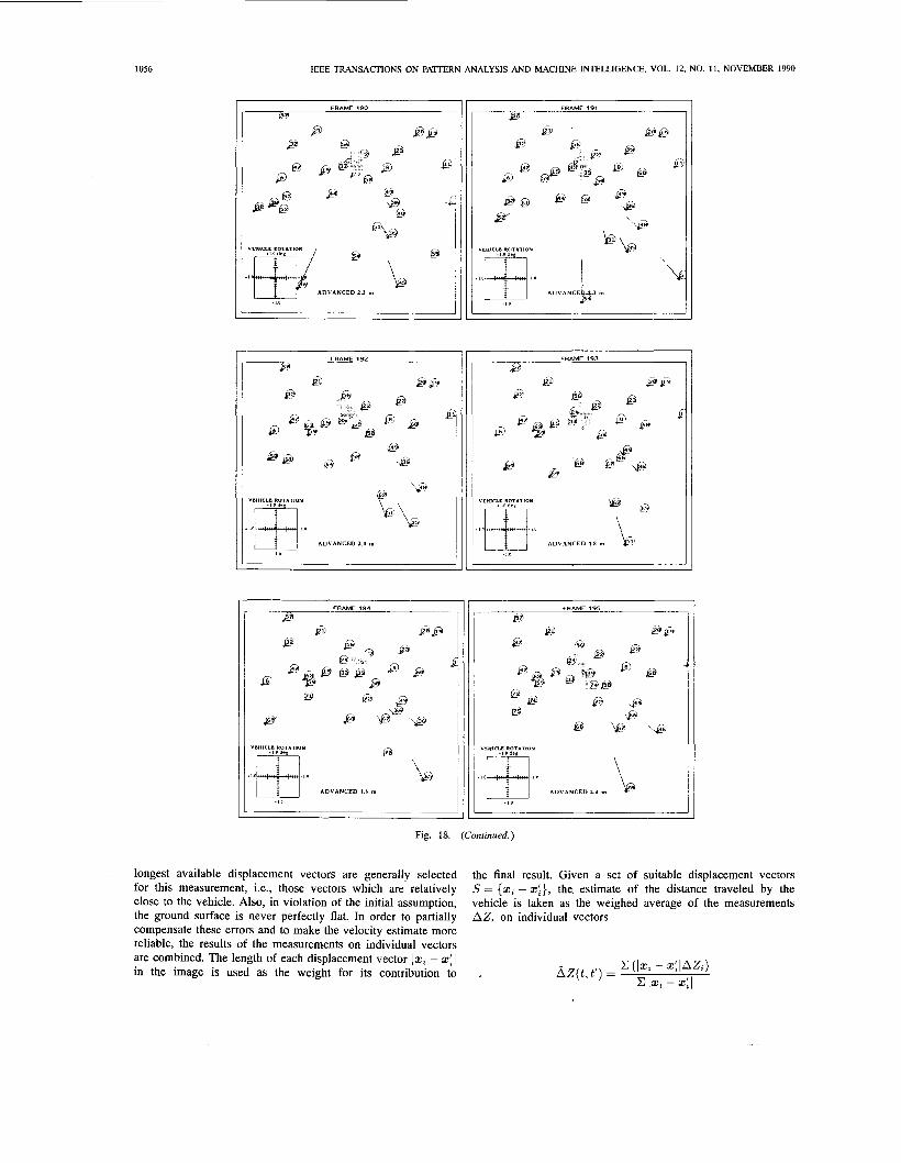
Fig. 18. Displacement vectors and estimates of vehicle motion for the ALV image sequence shown in Fig. 16. The shaded area in each image marks the computed fuzzy FOE, whose shape depends upon the most dominant (i.e., longest) displacement vectors. The small circle inside the shaded area is the FOE-location with minimum error. Estimated vehicle rotation is plotted in a coordinate frame in the range over *l.Oo. The estimated absolute advancement for each frame pair is given in meters. Original and demtated displacement vectors are drawn with solid and dotted lines, respectively.

For points on the road surface, the Y-coordinate is -h which is the height of the camera above ground. Therefore, the value of n, for a point on the road surface (xSy,) can be estimated as

-h U, =

yB cos er + f sin 8,


FRAME 184

VEHICLE ROTITION . I 0 d e l

ADVANCED 18 m

.!"H-" i o

- 1 0

FRAME 185

I I

I I F R A M E 186 F R A M E 187 I

F R A M E 188

la F R A M E 189

Fig. 18. (Continued. )

and its 3-D distance is found by inserting v, into the above equation as

at t and 2: at t' yield the amount of advancement AZ,(t, t') and estimated velocity V,(t, t') in this period as

If a point on the ground is observed at two instances of time, z, at time t and at t', the resulting distances from the vehicle 2,

Of course, image noise and tracking errors have a large impact upon the quality of the final velocity estimate. Therefore, the

1056

I FRAME 192

IEEE TRANSACTIONS ON PAlTERN ANALYSIS AND MACHINE INTELLIGENCE, VOL. 12, NO. 11, NOVEMBER 1990

FRAME 190

k?

ADVANCED 1.0 m

'@ Q YCHICLE ROTATION . , " I r e

A D V A N C E D 1 8 m

longest available displacement vectors are generally selected for this measurement, i.e., those vectors which are relatively close to the vehicle. Also, in violation of the initial assumption, the ground surface is never perfectly flat. In order to partially compensate these errors and to make the velocity estimate more reliable, the results of the measurements on individual vectors are combined. The length of each displacement vector 12, - 2: I

the final result. Given a set of suitable displacement vectors S = {z8 - z:}, the estimate of the distance traveled by the vehicle is taken as the weighed average of the measurements AZ, on individual vectors

( 1 2 2 - .:lAzJ Iz, - z:I

in the image is used as the weight for its contribution to , A Z ( t , t ' ) =

BURGER AND BHANU. ESTIMATING 3-D EGOMOTION 1057

@ @ 8 e ‘”

Y t IMAGE

Dl A N F

FRAME 197

Fig. 18. (Continued.)

GROUND c a a

3z, : * zo Fig. 19. Side view of the camera traveling parallel to a flat surface. The camera advanced in direction Z, such that a 3-D point on the ground moves relative to the camera from Zo to Z1. The depression angle 4 can be found from the location of the FOE in the image. The height of the camera above the ground is given.

and the final estimate for the vehicle velocity is

A2 V(t , t ’ ) = -. t’ - t This computation was applied to a sequence of real images shown in Section IV.

REFERENCES

[ 11 G. Adiv, “Determining three-dimensional motion and structure from optical flow generated by several moving objects,” IEEE Trans. Pattern Anal. Machine Intell., vol. PAMI-7, no. 4,

[2] P. Anandan, “Computing dense displacement fields with confidence measures in scenes containing occlusion,” SPIE Infell. Robots Comput. Vision, vol. 521, pp. 184-194, 1984.

[3] A. Bandopadhay, B. Chandra, and D. N. Ballard, “Egomotion using active vision,” in Proc. IEEE Con$ Computer Vision and Pattern Recognition, 1986, pp. 498- 503.

[4] S. T. Barnard and W. B. Thompson, “Disparity analysis of images,” IEEE Trans. Pattern Anal. Machine Intell., vol. PAMI-2, no. 4,

[5] B. Bhanu and W. Burger, “DRIVE-Dynamic reasoning from in- tegrated visual evidence,” Honeywell Systems & Research Center, Minneapolis, MN, DARPA Rep. DACA 76-86-C-0017, June 1987.

[6] -, “Qualitative motion detection and tracking of targets from a mobile platform,” in Proc. DARPA Image Understanding Workshop, Apr. 1988, pp. 289-318.

pp. 384-401, 1985.

pp. 333-340, July 1980.

[7] B. Bhanu, P. Symosek, J. Ming, W. Burger, H. Nasr, and J. Kim, “Qualitative target motion detection and tracking,” in Proc. DARPA Image Understanding Workshop. Morgan Kaufmann, May 1989.

[8] S. Bharwani, E. Riseman, and A. Hanson, “Refinement of environmental depth maps over multiple frames,” in Proc. IEEE Workshop Motion, Kiawah Island, SC, May 1986, pp. 73-80.

[9] T. J. Broida and R. Chellappa, “Estimation of object motion parameters from noisy images,” IEEE Trans. Pattern Anal. Machine Intell., vol. PAMI-8, no. 1, pp. 90-99, Jan. 1986.

[ lo] A. R. BNSS and B. K. P. Horn, “Passive navigation,” Comput. Vision, Graphics, Image Processing, vol. 21, pp. 3-20, 1983.

[ l l ] W. Burger and B. Bhanu, “Qualitative motion understanding,” in Proc. Tenth Int. Joint Con$ Artijicial Intelligence, IJCAI-87, Milan, Italy, Morgan Kaufmann, Aug. 1987.

[12] -, “Dynamic scene understanding for autonomous mobile robots,” in Proc. IEEE Con$ Computer Vision and Pattern Recognition, June 1988, pp. 736-741.

[13] -, “On computing a ‘fuzzy’ focus of expansion for autonomous navigation,” in Proc. IEEE Conj Computer Vision and Pattern Recognition, June 1989, pp. 563-568.

[14] J.Q. Fang and T.S. Huang, “Some experiments on estimating the 3-D motion parameters of a rigid body from two consecutive image frames,” IEEE Trans. Pattern Anal. Machine Intelligence, vol. PAMI-6, no. 5, pp. 54.5-554, Sept. 1984.

[15] 0. D. Faugeras, F. Lustman, and G. Toscani, “Motion and structure from point and line matches,” in Proc. 1st Int. Conj Computer Vision, June 1987, pp. 25-34.

[16] R. M. Haralick, “Using perspective transformations in scene analysis,” Comput. Graphics Image Processing, vol. 13, pp. 191 -221, 1980.

[17] C. Jerian and R. Jain, “Determining motion parameters for scenes with translation and rotation,” IEEE Trans. Pattern Anal. Machine Intell., vol. PAMI-6, no. 4, pp. 523-530, July 1984.

[18] J. Kim and B. Bhanu, “Motion disparity analysis using adap- tive windows,” Honeywell Systems & Research Center, Tech. Rep. 87SRC38, June 1987.

[ 191 D. T. Lawton, “Processing translational motion sequences,” Com- put. Vision, Graphics, Image Processing, vol. 22, pp. 114-116, 1983.

[20] D. N. h e , “The optic flow field: The foundation of vision,” Phil. Trans. Roy. Soc. London B, vol. 290, pp. 169-179, 1980.

[21] H. C. Longuet-Higgins, “A computer algorithm for reconstructing a scene from two projections,” Nature, vol. 293, pp. 133 - 135, Sept. 1981.

[22] H. C. Longuet-Higgins and K. Prazdny, “The interpretation of a moving retinal image,” Proc. Roy. Soc. London B, vol. 208,

[23] H. P. Moravec, “Towards automatic visual obstacle avoidance,” in Proc. 5th Int. Joint Conj Artificial Intelligence, Aug. 1977, p. 584.

[24] K. Prazdny, “Determining the instantaneous direction of motion from optical flow generated by a curvilinear moving observer,” Comput. Graphics Image Processing, vol. 17, pp. 238-248, 1981.

[25] D. Regan, K. Beverly, and M. Cynader, “The visual perception of motion in depth,” Sci. Amer., pp. 136-151, July 1979.

pp. 38.5-397, 1980.

1058 IEEE TRANSACTIONS ON PAITERN ANALYSIS AND MACHINE INTELLIGENCE, VOL. 12, NO. 11, NOVEMBER 1990

[26] J. H. Rieger, “Information in optical flows induced by curved paths of observation,” J. Opt. Soc. Amer., vol. 73, no. 3, pp. 339-344, Mar. 1983.

[27] J. H. Rieger and D. T. Lawton, “Processing differential image motion,” J. Opt. Soc. Amer. A, vol. 2, no. 2, pp. 354-360, Feb. 1985.

[28] J. W. Roach and J. K. Aggarwal, “Determining the movements of objects from a sequence of images,” IEEE Trans. Pattern Anal. Machine Intell., vol. PAMI-2, no. 6, pp. 554-562, 1980.

[29] B. G. Schunck, “Image flow: Fundamentals and future research,” in Proc. IEEE Con$ Computer Vision and Pattern Recognition, June

[30] R. Y. Tsai and T. S. Huang, “Uniqueness and estimation of three- dimensional motion parameters of rigid objects with curved sur- faces,” IEEE Trans. Pattern Anal. Machine Intell., vol. PAMI-6, no. 1, pp. 13-27, Jan. 1984.

[31] S. Ullman, The Interpretation of Visual Motion. Cambridge, MA: MIT Press, 1979.

[32] A. Verri and T. Poggio, “Qualitative information in the optical flow,’’ in Proc. DAREA Image Understanding Workshop, Los An- geles, CA, Feb. 1987, pp. 825-834.

[33] J. Weng, T.S. Huang, and N. Ahuja, “Error analysis of motion parameter estimation from image sequences,” in Proc. 1st Int. Con$ Computer Vision, June 1987, pp. 703-707.

1985, pp. 560-571.

Wilhelm Burger was born in Austria in 1955. He received the undergraduate degree from Johannes Kepler University, Linz, Austria, in 1983 and the M.S. degree in computer science from the University of Utah, Salt Lake City, in 1987. He is currently working toward the Doctoral degree in the area of freeform object recognition and representation.

From 1975 to 1981 he was employed as a system engineer with Kretztechnik Ultrasound, Austria, where he develoDed imagine hardware

for medical ultrasound scanners. During 1986 -1687 he Gas Research Associate in the Signal and Image Processing group at the Honeywell Systems and Research Center in Minneapolis, MN, where he did work in motion analysis for autonomous vehicle navigation. Since 1987 he has been a faculty member at the Institute of Systems Science at Johannes Kepler University Linz, where he is involved in teaching and research in the area of machine vision. His primary research interests include motion analysis, inexact approaches in vision, freeform object recognition, robust feature extraction, machine learning, and hardwarehoftware environments for image understanding.

Bir Bhanu (S’72 - M’82 - SM’87) received the B.S. degree (with Honors) in electronics engineering from the Indian Institute of Technology (BHU), Varanasi, India, the M.E. degree (with Distinction) in electronics engineering from Birla Institute of Technology and Science, Pilani, India, the S.M. and E.E. degrees in electrical engineering and computer science from the Massachusetts Institute of Technology, Cambridge, the Ph.D. degree in electrical engineering from the Image Pro-

cessing Institute, University of Southern California, Los Angeles, and the M.B.A. degree from the University of California, Irvine. He also received the Diploma in German from BHU, Varanasi, India.

He is a Honeywell Fellow at Honeywell Systems and Research Center, where he serves as the Principal Investigator of the Scene Dynamics Program from DARPA, the Obstacle Detection Program from NASA, and the Machine Learning Program from a government agency. Additionally, he is conducting sponsored and IR&D research efforts on machine learning, robotic vehicle navigation, target recognition and tracking, object modeling, contextual analysis, multisensor integration, parallel algorithms, scientific performance evaluation of image understanding algorithmshystems, and photointerpretation and surveillance. He has also worked with IBM on image processing, INRIA-France on 3-D object recognition and Ford Aerospace and Communications Corporation on automatic target recognition. While on the faculty of the Department of Computer Science, University of Utah, he was the Principal Investigator on several NSF and industry funded research projects in machine intelligence. His current interests are computer vision, robotics, machine learning, neural networks and neurocomputers, object modeling, multisensor integration, distributed sensing and control, parallel computer architectures, and applications of artificial intelligence.

Dr. Bhanu has over 100 reviewed technical publications and 5 patents in the areas of his interest. He has given national short courses on intelligent automatic target recognition. He is a reviewer to over two dozen technical publications and government agencies. He was the Guest Editor of a special issue of IEEE Computer on “CAD-Based Robot Vision” published in August 1987. He is listed in the American Men and Women of Science, Who’s Who in the West, Personalities of Americas and 5000 Personalities of the World. He is a member of ACM, AAAI, Sigma Xi, Pattern Recognition Society, SPIE, and the IEEE Computer Society.

1040 no. estimating 3-d egomotion perspective … and conference papers...1040 ieee transactions on...

Documents