10.*: the theory of hypothesis testing

STAT200: Introductory Statistics

§10.*: The Theory ofHypothesis Testing

Objectives

By the end of this lecture, you should be able to1 be able to identify the research, null, and alternative hypotheses2 calculate the p-value for a given alternative hypothesis3 properly interpret the p-value

STAT200: Introductory Statistics 10.*: The Theory of Hypothesis Testing 2

The Arc

Previously, wecalculated confidence intervalsinterpreted confidence intervals

Today, we will examinehypothesis testing and p-values


The Theory

The theory behind hypothesis testing is

1 State the research hypothesis and the null hypothesis

2 Determine how much the data support the hypothesis:Determine the parameter testedDetermine appropriate statisticDetermine distribution of that statistic under the nullDetermine how likely it is to observe the statistic (data) if thenull hypothesis is true

3 Interpret that level of support


Definitions: Hypotheses

Definition (Hypothesis)A hypothesis is a testable claim about reality.

Since it is a claim about reality, it concerns some aspect of thepopulation (a parameter). The usual parameters hypothesized aboutat this level are the mean µ, proportion p, and variance σ2. BUT wecan hypothesize about any aspects of the population.

The “generic” parameter is θ.

Since it is a claim about reality, it separates all possible realities intothose that are consistent with the hypothesis and those that areincompatible with it.



The most important hypothesis is the one made by the researcher:

Definition (Research Hypothesis)A research hypothesis is a testable claim about reality made by thescientist.

This is the one that the statistician must eventually come to aconclusion about.

Because we are using statistics to test this hypothesis, we create twostatistics-specific hypotheses. These two hypotheses divide all possiblerealities into two groups, those that are a part of the research andthose that are not.



HR H0 HA

θ < θ0 θ ≥ θ0 θ < θ0θ = θ0 θ = θ0 θ 6= θ0θ > θ0 θ ≤ θ0 θ > θ0

θ ≤ θ0 θ ≤ θ0 θ > θ0θ 6= θ0 θ = θ0 θ 6= θ0θ ≥ θ0 θ ≥ θ0 θ < θ0

Table: A listing of all possible research hypotheses and their corresponding nulland alternative hypotheses.

The symbol θ is a generic parameter. It can represent µ, p, σ2, or anyother parameter you can imagine.

The symbol θ0 represents the value claimed by the researcher. Itis a number.Do not memorize this table. Learn what it says about therelationships between the research and other hypotheses. . . andbetween the null and alternative hypotheses. What do all of thenull hypotheses have in common?(Why would that be a requirement?) What is the relationshipbetween the null and alternative hypotheses?(Why does this make sense?)


Definitions: p-value

Definition (p-value)The p-value is the probability of observing a test statistic thisextreme, or more so, given the null hypothesis is true.

Definition (p-value)The p-value is the probability of observing data this extreme, ormore so, given the null hypothesis is true.

Definition (p-value)The p-value is the amount of support in the data for the nullhypothesis.


Definitions: Decision Theory

We now have two of the three parts of the “hypothesis-testing theory”laid out earlier. The last part is making a decision about the researchhypothesis based on the data.

Do the data sufficiently support the research hypothesis?

Note that the very statement is binary: Yes or No.

Since the decision is binary, we need to determine a ‘cut-off’ pointbetween what supports the research hypothesis and what does not.This boundary is referred to as “the alpha-value.”

If the level of support is less than alpha, we reject the null hypothesis.Otherwise, we do not (we fail to reject).



Definition (alpha-value)The alpha value is the Type I error rate claimed by the statistician.

Definition (Type I error)A Type I error occurs when the researcher rejects a true nullhypothesis.

Definition (Type I error rate)The Type I error rate is the proportion of the time the researchercommits a Type I error (rejects a true null hypothesis).

Note: The actual Type I error rate may not be α. LaboratoryActivity F explores this in greater detail.



If there is a Type I error, then there must be (at least) a Type II error.

Definition (Type II error)A Type II error occurs when the researcher fails to reject a falsenull hypothesis. Its value is symbolized by β.

Both are error rates. So, we would like to minimize both. However,decreasing α results in increasing β.

Furthermore, reducing either to zero results in the other being 100%.

Sadness abounds.


Definitions: Decision Theory (aside)

If there is a Type I error, then there must be (at least) a Type II error.There are, in fact, a couple more (non-standard) types of errors. Theydo, however, give some more insight into what can go wrong instatistical analysis.

Definition (Type III error)A Type III error occurs when the researcher rejects a false nullhypothesis, but for the wrong reason.

Remember: This is not standard terminology.


Definitions: Decision Theory (aside)

Definition (Type III error)A Type III error occurs when the researcher rejects a false nullhypothesis, but for the wrong reason.

Causes of Type III errors include:wrong testaggregation biasecological fallacycollinearity among predictors

The key to avoiding Type III errors is to fully understandthe statistical tests. The wrong test or the wronginterpretation or the wrong assumptions all lead toerrors.


Exploratory Example 1: CCD1, Coins

Example

I would like to test if my coin is biased in favor of getting heads.Specifically, using statistical language, my research hypothesis is

HR : p > 0.500

To test this, I flip the coin 100 times and get 58 heads.

If the research hypothesis is “>,” then the null is “≤.”From the problem set-up, we know that the number of heads, X

is distributed as X ∼ Bin(n = 100; p = 0.500) — if the coin is fair.Also, if the the number of observed heads is too large, we know

that the alternative hypothesis is more likely to be correct.So, let’s calculate the p-value:

The p-value is the probability of observing data this extreme— or more so — given the null hypothesis is true.

Thus, it is P[X ≥ 58 | X ∼ Bin(100; 0.500)

].

Being specific,p-value = P

[X ≥ 58 | X ∼ Bin(100; 0.500)

]=

= 1 - pbinom(57, size=100, prob=0.500) = 0.06660531Thus, the probability of observing data this extreme (or more so),given the null hypothesis is true, isP[X ≥ 58 | X ∼ Bin(100; 0.500)

]= 0.06660531

What does this mean??


Exploratory Example 1: CCD1, Coins

This is the probability mass function of the number of heads, X,given the null hypothesis is true.

The dark-shaded values are the probabilities corresponding to valuesas extreme — or more so — as what was observed, given thedistribution of the number of heads.

— Their sum is the p-value.


Exploratory Example 2: CCD2, Cards

Example

I believe that my blackjack dealer is cheating. If everything is fair,then I would expect to have a blackjack 4.75% of the time. I haveplayed n = 132 hands and got a blackjack only once. Is this fair?Specifically, using statistical language, my research hypothesis (claim)is

HR : p < 0.0475

If the research hypothesis is “<,” then the null is “≥.”From the problem set-up, we know that the number of blackjacks,

X is distributed as X ∼ Bin(n = 132; p = 0.0475) — if the dealer isfair. Also, if the the number of observed blackjacks is too small, weknow that the alternative hypothesis is more likely to be correct.So, let’s calculate the p-value:


Thus, it is P[X ≤ 1 | X ∼ Bin(132; 0.0475)

].

p-value = P[X ≤ 1 | X ∼ Bin(132; 0.0475)

]= pbinom(1, size=132, prob=0.0475)

= 0.0123027

Thus, the probability of observing data this extreme (or more so),given the null hypothesis is true, isP[X ≤ 1 | X ∼ Bin(132; 0.0475)

]= 0.0123027



Exploratory Example 2: CCD2, Cards

This is the probability mass function of the number of blackjacks, X,given the null hypothesis is true.

The dark-shaded values are the probabilities corresponding to valuesas extreme — or more so — as what was observed, given thedistribution of the number of heads.



Exploratory Example 3: CCD3, Dice

Example

I believe that this die is biased against getting a 6. Specifically, usingstatistical language, my research hypothesis (claim) is

HR : p < 0.1667

To test this, I roll the die 100 times and get a 6 a total of 9 times.

If the research hypothesis is “<,” then the null is “≥.”From the problem set-up, we know that the number of sixes, X is

distributed as X ∼ Bin(n = 100; p = 0.1667) — if the die is fair.Also, if the the number of observed sixes is too small, we know

that the alternative hypothesis is more likely to be correct.So, let’s calculate the p-value:


Thus, it is P[X ≤ 9 | X ∼ Bin(100; 0.1667)

].

Being specific,p-value = P

[X ≤ 9 | X ∼ Bin(100; 0.1667)

]=

= pbinom(9, size=100, prob=0.1667) = 0.02124964Thus, the probability of observing data this extreme (or more so),given the null hypothesis is true, isP[X ≤ 9 | X ∼ Bin(100; 0.1667)

]= 0.02124964



Exploratory Example 3: CCD3, Dice

This is the probability mass function of the number of sixes, X, giventhe null hypothesis is true.

The dark-shaded values are the probabilities corresponding to valuesas extreme — or more so — as what was observed, given thedistribution of the number of sixes.



Example 1

Example

Wacdnalds claims that the weight of a quarter-pounder hamburgerpatty (before cooking) is 4 ounces, with a standard deviation of σ = 1ounce. In symbols, this is

HR : µ = 4

To test this, we weigh a stack of n = 25 patties and find that the totalweight is only 94 ounces.

Is there sufficient evidence that Wacdnalds is incorrect?We seek to calculate P[T ≤ 94 or T ≥ 106], whereT ∼ N (100; σ = 1

√25).

This isp-value = 2 * pnorm(94, m=100, s=5) = 0.2301393

How should we interpret this result?


Example 1

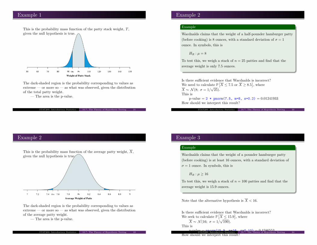
This is the probability mass function of the patty stack weight, T ,given the null hypothesis is true.

The dark-shaded region is the probability corresponding to values asextreme — or more so — as what was observed, given the distributionof the total patty weight.

— The area is the p-value.


Example 2

Example

Wacdnalds claims that the weight of a half-pounder hamburger patty(before cooking) is 8 ounces, with a standard deviation of σ = 1ounce. In symbols, this is

HR : µ = 8

To test this, we weigh a stack of n = 25 patties and find that theaverage weight is only 7.5 ounces.

Is there sufficient evidence that Wacdnalds is incorrect?We need to calculate P

[X ≤ 7.5 or X ≥ 8.5

], where

X ∼ N (8; σ = 1/√

25).This is

p-value = 2 * pnorm(7.5, m=8, s=0.2) = 0.01241933How should we interpret this result?


Example 2

This is the probability mass function of the average patty weight, X,given the null hypothesis is true.

The dark-shaded region is the probability corresponding to values asextreme — or more so — as what was observed, given the distributionof the average patty weight.



Example 3

Example

Wacdnalds claims that the weight of a pounder hamburger patty(before cooking) is at least 16 ounces, with a standard deviation ofσ = 1 ounce. In symbols, this is

HR : µ ≥ 16

To test this, we weigh a stack of n = 100 patties and find that theaverage weight is 15.9 ounces.

Note that the alternative hypothesis is X < 16.

Is there sufficient evidence that Wacdnalds is incorrect?We seek to calculate P

[X ≤ 15.9

], where

X ∼ N (16; σ = 1/√

100).This is

p-value = pnorm(15.9, m=16, s=0.10) = 0.1586553How should we interpret this result?


Example 3

This is the probability mass function of the average patty weight, X,given the null hypothesis is true.

The dark-shaded region is the probability corresponding to values asextreme — or more so — as what was observed, given the distributionof the average patty weight.



Example 4

Example

Wacdnalds claims that the number of Calories in a McPork is at most350, with a standard deviation of σ = 50 Calories. In symbols, this is

HR : µ ≤ 350

To test this, we perform a calorimetry test on a stack of n = 100McPorks and find that the average number of Calories is 343.

Note that the alternative hypothesis is X > 343.

Is there sufficient evidence that Wacdnalds is incorrect?We are asked to calculate P

[X ≥ 343

], where

X ∼ N (350; σ = 50/√

100).This is

p-value = 1-pnorm(343, m=350, s=5) = 0.9192433How should we interpret this result?


Example 3: Wacdnalds

This is the probability mass function of the average Calories in theMcPork, X, given the null hypothesis is true.

The dark-shaded region is the probability corresponding to values asextreme — or more so — as what was observed, given the distributionof the average Calories.



Today’s Summary

In today’s slide deck, we coveredstating hypothesestesting hypothesescalculating p-value from definition


R Functions

Here is what we used the following R functions:

pnorm(x, m,s)

pbinom(x, size,prob)

Please do not forget to download the allProcedures.pdf file thatlists all of the statistical procedures we will use in R.


The Future

In the future, we will. . .Review todayUse R to calculate the confidence intervals easily

Also in the future, we will see many, many, many more tests.Make sure you keep a separate sheet for what they are, whenthey are useful, what the analysis procedures are, and how to dothem in R.


Readings

Course Readings:R for Starters: Chapter 4Hawkes Learning: Chapter 10

Supplementary ReadingsWikipedia: Hypothesis Tests


STAT200: Introductory Statistics

§10.*: The Theory ofHypothesis Testing

Ole J. ForsbergAssistant Professor of Mathematics - StatisticsKnox College, Galesburg, [email protected]

10.*: the theory of hypothesis testing

Documents