10 statisticalmethodsfor astronomypersonal.psu.edu/gjb6/mypdfpap/2013springerplanets.pdf · 10...
TRANSCRIPT

10 Statistical Methods forAstronomyEric D. Feigelson, ⋅ G. Jogesh Babu,Department of Astronomy & Astrophysics,The Pennsylvania StateUniversity, University Park, PA, USADepartment of Statistics, The Pennsylvania State University,University Park, PA, USACenter for Astrostatistics,The Pennsylvania State University,University Park, PA, USA
1 Role and History of Statistics in Astronomy . . . . . . . . . . . . . . . . . . . . . . . . . . . . . 446
2 Statistical Inference . . . . . . . . . . . . . . . . . . . . . . . . . . . . . . . . . . . . . . . . . . . . . . . . 4502.1 Concepts of Statistical Inference . . . . . . . . . . . . . . . . . . . . . . . . . . . . . . . . . . . . . . . . . 4502.2 Probability Theory and Probability Distributions . . . . . . . . . . . . . . . . . . . . . . . . . . . 4512.3 Point Estimation . . . . . . . . . . . . . . . . . . . . . . . . . . . . . . . . . . . . . . . . . . . . . . . . . . . . . . 4542.4 Least Squares . . . . . . . . . . . . . . . . . . . . . . . . . . . . . . . . . . . . . . . . . . . . . . . . . . . . . . . . 4552.5 Maximum Likelihood Method . . . . . . . . . . . . . . . . . . . . . . . . . . . . . . . . . . . . . . . . . . 4552.6 Hypotheses Tests . . . . . . . . . . . . . . . . . . . . . . . . . . . . . . . . . . . . . . . . . . . . . . . . . . . . . 4572.7 Bayesian Estimation . . . . . . . . . . . . . . . . . . . . . . . . . . . . . . . . . . . . . . . . . . . . . . . . . . . 4572.8 Resampling Methods . . . . . . . . . . . . . . . . . . . . . . . . . . . . . . . . . . . . . . . . . . . . . . . . . . 4592.9 Model Selection and Goodness of Fit . . . . . . . . . . . . . . . . . . . . . . . . . . . . . . . . . . . . . 4602.10 Nonparametric Statistics . . . . . . . . . . . . . . . . . . . . . . . . . . . . . . . . . . . . . . . . . . . . . . . 461
3 Applied Fields of Statistics . . . . . . . . . . . . . . . . . . . . . . . . . . . . . . . . . . . . . . . . . . 4643.1 Data Smoothing . . . . . . . . . . . . . . . . . . . . . . . . . . . . . . . . . . . . . . . . . . . . . . . . . . . . . . 4643.2 Multivariate Clustering and Classification . . . . . . . . . . . . . . . . . . . . . . . . . . . . . . . . . 4653.3 Nondetections and Truncation . . . . . . . . . . . . . . . . . . . . . . . . . . . . . . . . . . . . . . . . . . 4683.4 Time Series Analysis . . . . . . . . . . . . . . . . . . . . . . . . . . . . . . . . . . . . . . . . . . . . . . . . . . 4693.5 Spatial Point Processes . . . . . . . . . . . . . . . . . . . . . . . . . . . . . . . . . . . . . . . . . . . . . . . . . 472
4 Resources . . . . . . . . . . . . . . . . . . . . . . . . . . . . . . . . . . . . . . . . . . . . . . . . . . . . . . . 4734.1 Web Sites and Books . . . . . . . . . . . . . . . . . . . . . . . . . . . . . . . . . . . . . . . . . . . . . . . . . . 4754.2 The R Statistical Software System . . . . . . . . . . . . . . . . . . . . . . . . . . . . . . . . . . . . . . . . 475
Acknowledgments . . . . . . . . . . . . . . . . . . . . . . . . . . . . . . . . . . . . . . . . . . . . . . . . . . . . . . 478
References . . . . . . . . . . . . . . . . . . . . . . . . . . . . . . . . . . . . . . . . . . . . . . . . . . . . . . . . . . . . 478
T.D. Oswalt, H.E. Bond (eds.), Planets, Stars and Stellar Systems. Volume 2: Astronomical Techniques, Software,and Data, DOI 10.1007/978-94-007-5618-2_10, © Springer Science+Business Media Dordrecht 2013

446 10 Statistical Methods for Astronomy
Abstract: Statistical methodology, with deep roots in probability theory, provides quantitativeprocedures for extracting scientific knowledge from astronomical data and for testingastrophysical theory. In recent decades, statistics has enormously increased in scope and sophis-tication. After a historical perspective, this review outlines concepts of mathematical statistics,elements of probability theory, hypothesis tests, and point estimation. Least squares, maxi-mum likelihood, and Bayesian approaches to statistical inference are outlined. Resamplingmethods, particularly the bootstrap, provide valuable procedures when distributions functionsof statistics are not known. Several approaches to model selection and goodness of fit areconsidered.
Applied statistics relevant to astronomical research are briefly discussed. Nonparametricmethods are valuable when little is known about the behavior of the astronomical populationsor processes. Data smoothing can be achieved with kernel density estimation and nonpara-metric regression. Samples measured in many variables can be divided into distinct groupsusing unsupervised clustering or supervised classification procedures. Many classification anddata mining techniques are available. Astronomical surveys subject to nondetections can betreated with survival analysis for censored data, with a few related procedures for truncateddata. Astronomical light curves can be investigated using time-domain methods involving theautoregressive models, frequency-domain methods involving Fourier transforms, and state-space modeling. Methods for interpreting the spatial distributions of points in some space havebeen independently developed in astronomy and other fields.
Two types of resources for astronomers needing statistical information and tools are pre-sented. First, about 40 recommended texts and monographs are listed covering various fieldsof statistics. Second, the public domain R statistical software system has recently emerged asa highly capable environment for statistical analysis. Together with its ∼3,000 (and growing)add-onCRAN packages,R implements a vast range of statistical procedures in a coherent high-level language with advanced graphics. Two illustrations of R’s capabilities for astronomicaldata analysis are given: an adaptive kernel estimator with bootstrap errors applied to a quasardataset, and the second-order J function (related to the two-point correlation function) withthree edge corrections applied to a galaxy redshift survey.
Keywords: Astrostatistics; Bayesian inference; Bootstrap resampling; Censoring (upper lim-its); Data mining; Goodness of fit tests; Hypothesis tests; Kernel density estimation; Leastsquares estimation; Maximum likelihood estimation; Model selection; Multivariate classifica-tion; Nonparametric statistics; Probability theory; R (statistical software); Regression; Spatialpoint processes; Statistical inference; Statistical software; Time series analysis; Truncation
1 Role and History of Statistics in Astronomy
Through much of the twentieth century, astronomers generally viewed statistical methodologyas an established collection of mechanical tools to assist in the analysis of quantitative data.A narrow suite of classical methods were commonly used, such as model fitting by minimizinga χ-like statistic, goodness of fit tests of a model to a dataset with the Kolmogorov–Smirnovstatistic, and Fourier analysis of time series. These methods are often used beyond their rangeof applicability. Except for a vanguard of astronomers expert in specific advanced techniques(e.g., Bayesian or wavelet analysis), there was little awareness that statistical methodology had

Statistical Methods for Astronomy 10 447
progressed considerably in recent decades to provide a wealth of techniques for wide range ofproblems. Interest in astrostatistics and associatedfields like astroinformatics is rapidly growingtoday.
The role of statistical analysis as an element of scientific inference has been widely debated(Rao 1997). “Statistics” originally referred to the collection and rudimentary characterizationof empirical data. In recent decades, it has accrued othermeanings: inference beyond the datasetto the underlying populations under study, quantification of uncertainty in the data, induc-tion of mechanisms causing patterns in the data, and assistance in making decisions based onthe data.
Some statisticians feel that, while statistical characterization canbe effective, statisticalmod-eling is oftenunreliable. StatisticianG. E. P. Box famously said “Essentially, allmodels arewrong,but some are useful,” and Sir D. R. Cox (2006) wrote “The use, if any, in the process of simplequantitative notions of probability and their numerical assessment [to scientific inference] isunclear.” Others are more optimistic. Astrostatistician P. C. Gregory (2005) writes:
Our [scientific] understanding comes through the development of theoretical modelswhich are capable of explaining the existing observations as well as making testablepredictions. … Fortunately, a variety of sophisticated mathematical and computationalapproaches have been developed to help us through this interface, these go under thegeneral heading of statistical inference.
Astronomersmight distinguish cases where themodel has a strong astrophysical underpin-ning (such as fitting a Keplerian ellipse to a planetary orbit) and cases where the model doesnot have a clear astrophysical explanation (such as fitting a power law to the distribution of stel-lar masses). In all cases, astronomers should carefully formulate the question to be addressed,apply carefully chosen statistical approaches to the dataset to address this question with clearlystated assumptions, and recognize that the link between the statistical findings and reality maynot be straightforward.
Prior to the twentieth century, many statistical developments were centered around astro-nomical problems (Stigler 1986). Ancient Greek, Arabic, and Renaissance astronomers debatedhow to estimate a quantity, such as the length of a solar year, based on repeated and incon-sistent measurements. Most favored the middle of the extreme values, and some scholarsfeared that repeated measurement led to greater, not reduced, uncertainty. The mean was pro-moted by Tycho Brahe and Galileo Galilei, but did not become the standard procedure untilthe mid-eighteenth century. The eleventh century Persian astronomer al-Biruni and Galileodiscussed propagation of measurement errors. Adrian Legendre and Carl Friedrich Gaussdeveloped the “Gaussian” or normal error distribution in the early nineteenth century to addressdiscrepant measurement in celestial mechanics. The normal distribution was intertwined withthe least-squares estimation technique developedby Legendre and Pierre-Simon Laplace. Lead-ing astronomers throughout Europe contributed to least-squares theory during the nineteenthcentury.
However, the close association of statistics with astronomy atrophied during the beginningof the twentieth century. Statisticians focused their attention on biological sciences and humanaffairs: biometrics, demography, economics, social sciences, industrial reliability, and processcontrol. Astronomers made great advances by applying newly developed fields of physics toexplain astronomical phenomena.The structure of a star, for example, was powerfully explainedby combining gravity, thermodynamics, and atomic and nuclear physics. During the middle

448 10 Statistical Methods for Astronomy
of the century, astronomers continued using least-squares techniques, although heuristic pro-cedures were also common. Astronomers did not adopt the powerful methods of maximumlikelihood estimation (MLE), formulated by Sir R. A. Fisher in the 1920s and widely promul-gated in other fields.MLE came into use during the 1970s–1980s, along with the nonparametricKolmogorov–Smirnov statistic. Practical volumes by Bevington (1969) and Press et al. (1986)with Fortran source codes promulgated a suite of classical methods.
The adoption of a wider range of statistical methodology began during the 1990s andis still growing. Sometimes developments were made independently of mathematical statis-tics; for example, development of the two-point correlation function to study galaxy clus-tering was largely independent of the closely related mathematical developments relating toRipley’s K function for non-random spatial point processes. Progress was made in developingprocedures for analyzing unevenly spaced time series and populations from truncated (flux-limited) astronomical surveys, problems that rarely arose in other fields. As computationalmethods advanced, parametric modeling using Bayesian analysis became attractive for a varietyof problems that are not satisfactorily addressed by traditional frequentists methods.
The 1990s also witnessed the emergence of cross-disciplinary interactions betweenastronomers and statisticians including collaborative research groups, conferences, didacticsummer schools, and software resources. A small but growing research field of astrostatis-tics was established. The activity is propelled both by the sophistication of data analysis andmodeling problems, and the exponentially growing quantity of publicly available astronom-ical data. Both primary and secondary data products are provided by organizations such asNASA’s Science Archive Research Centers, ground-based observatory archives, and databasessuch as NASA’s Extragalactic Database and SIMBAD. The NASA/Smithsonian AstrophysicsData System, a billion-hit Web site, is an effective portal to the astronomical research litera-ture and databases. The International Virtual Observatory that facilitates access to distributeddatabases will only increase the need for statistical resources to analyze multiwavelengthdatasets selectedby the astronomer for examination.These datasets are reaching petabyte scaleswith multivariate catalogs providing measured properties of billions of astronomical objects.
Thus, the past two centuries have witnessed the astronomical foundations of statistics, agrowing distance between the fields, and a recent renaissance in astrostatistics. The need for,and use of, advanced statistical techniques in the service of interpreting astronomical data andtesting astrophysical theory is now ascendent.
The purpose of this review is to introduce some of the concepts and results of a broad scopeof modern statistical methodology that can be effective for astronomical data and science anal-ysis. > Section 2 outlines concepts and results of statistical inference that underlie statisticalanalysis of astronomical data. >Section 3 reviews several fields of applied statistics relevant forastronomy. >Section 4 discusses resources available for the astronomer to learn appropriatestatistical methodology, including the powerful R software system. Key terminology is noted inquotationmarks (e.g., “bootstrap resampling”).The coverage is abbreviated and not complete inany fashion. Topics aremostly restricted to areas of established statistical methodology relevantto astronomy; recent advances in the astronomical literature aremostly not considered. Amorecomprehensive treatment for astronomers can be found in Feigelson and Babu (2012), and thevolumes listed in >Table 10-1 should be consulted prior to serious statistical investigations.

Statistical Methods for Astronomy 10 449
⊡ Table 10-1Selected statistics books for astronomers
Broad scope
Adler (2010) R in a Nutshell
Dalgaard (2008) Introductory Statistics with R
Feigelson and Babu (2012) Modern Statistical Methods for Astronomy with R
Applications
Rice (1994) Mathematical Statistics and Data Analysis
Wasserman (2005) All of Statistics: A Concise Course in Statistical Inference
Statistical inference
Conover (1999) Practical Nonparametric Statistics
Evans et al. (2000) Statistical Distributions
Hogg and Tanis (2009) Probability and Statistical Inference
James (2006) Statistical Methods in Experimental Physics
Lupton (1993) Statistics in Theory and Practice
Ross 2010 A First Course in Probability
Bayesian statistics
Gelman et al. (2004) Bayesian Data Analysis
Gregory (2005) Bayesian Logical Data Analysis for the Physical Sciences
Kruschke (2011) Doing Bayesian Data Analysis: A Tutorial with R andBUGS
Resampling methods
Efron and Tibshirani (1993) An Introduction to the Bootstrap
Zoubir and Iskander (2004) Bootstrap Techniques for Signal Processing
Density estimation
Bowman and Azzalini (1997) Applied Smoothing Techniques for Data Analysis
Silverman (1998) Density Estimation
Takezawa (2005) Introduction to Nonparametric Regression
Regression andmultivariate analysis
Kutner et al. (2004) Applied Linear Regression Models
Johnson and Wichern (2007) Applied Multivariate Statistical Analysis
Nondetections
Helsel (2004) Nondetects and Data Analysis
Klein and Moeschberger (2010) Survival Analysis
Lawless (2002) Statistical Models and Methods for Lifetime Data
Spatial processes
Bivand et al. (2008) Applied Spatial Data Analysis with R
Fortin and Dale (2005) Spatial Analysis: A Guide for Ecologists
Illian et al. (2008) Statistical Analysis and Modelling of Spatial PointPatterns
Martínez and Saar (2002) Statistics of the Galaxy Distribution
Starck and Murtagh (2006) Astronomical Image and Data Analysis
450 10 Statistical Methods for Astronomy
⊡ Table 10-1(Continued)
Data mining, clustering, and classification
Everitt et al. (2001) Cluster Analysis
Duda et al. (2001) Pattern Classification
Hastie et al. (2009) The Elements of Statistical Learning
Way et al. (2011) Advances in Machine Learning and Data Miningfor Astronomy
Time series analysis
Chatfield (2004) The Analysis of Time Series
Cowpertwait and Metcalfe (2009) Introductory Time Series with R
Nason (2008) Wavelet Methods in Statistics with R
Shumway and Stoffer (2006) Time Series Analysis and Its Applications with RExamples
Graphics and data visualization
Chen et al. (2008) Handbook of Data Visualization
Maindonald and Braun (2010) Data Analysis and Graphics using R
Sarkar (2008) Lattice: Multivariate Data Visualizationwith R
Wickham (2009) ggplot2: Elegant Graphics for Data Analysis
2 Statistical Inference
2.1 Concepts of Statistical Inference
A “random variable” is a function of potential outcomes of an experiment. A particularrealization of a random variable is often called a “data point.” The magnitude of stars orredshifts of galaxies are examples of random variables. An astronomical dataset might con-tain photometric measurements of a sample of stars, spectroscopic redshifts of a sample ofgalaxies, categorical measurements (such as radio-loud and radio-quiet active galactic nuclei),or brightness measurements as a function of sky location (an image), wavelength of light(a spectrum), or of time (a light curve).The datasetmight be very small so that large-N approx-imations do not apply, or very large making computations difficult to perform. Observed valuesmay be accompanied by secondary information, such as estimates of the errors arising from themeasurementprocess. “Statistics” are functions of random variables, ranging from simple func-tions, such as the mean value, to complicated functions, such as an adaptive kernel smootherwith cross-validation bandwidths and bootstrap errors (>Fig. 10-2 below).
Statisticians have established the distributional properties of a number of statistics throughformal mathematical theorems. For example, under broad conditions, the “Central Limit The-orem” indicates that the mean value of a sufficiently large sample of independent randomvariables is normally distributed. Astronomers can invent statistics that reveal some scientif-ically interesting properties of a dataset, but can not assume they follow simple distributionsunless this has been established by theorems. But in many cases, Monte Carlo methods such asthe bootstrap can numerically recover the distribution of the statistic from a particular datasetunder study.

Statistical Methods for Astronomy 10 451
Statistical inference, in principle, helps reach conclusions that extend beyond the imme-diate data to derive broadly applicable insights into the underlying population. The field ofstatistical inference is very large and can be classified in a number of ways. “Nonparametricinference” gives probabilistic statements about the data which do not assume any particulardistribution (e.g., Gaussian, power law) or parametric model for the data, while “parametricinference” assumes some distributions or functional relationships. These relationships can besimple heuristic relations, as in linear regression, or can be complex functions derived fromastrophysical theory. Inference can be viewed as the combination of two basic branches: “pointestimation” (such as estimating the mean of a dataset) and the “testing of hypotheses” (such asa 2-sample test on the equality of two medians).
It is important that the scientist be aware of the range of applicability of a given inferentialprocedure. Several problems relevant to astronomical statistical practice can bementioned. Var-ious statistics that resemble Pearson’s χ do permit a weighted least squares regression, but thestatistic often does not follow the χ distribution. The Kolmogorov–Smirnov statistic can be avaluable measure of difference between a sample and a model, but tabulated probabilities areincorrect if themodel is derived from that sample (Lilliefors 1969) and the statistic is ill-definedif the dataset is multivariate. The likelihood ratio test can compare the ability of two models toexplain a dataset, but it cannot be used if an estimated parameter value is consistent with zero(Protassov et al. 2002).
2.2 Probability Theory and Probability Distributions
Statistics is rooted in probability theory, a branch of mathematics seeking to model uncertainty(Ross 2010). Nearly all astronomical studies encounter uncertainty: observed samples representonly small fractions of underlying populations, properties of astrophysical interest aremeasuredindirectly or incompletely, errors are present due to themeasurement process.The theory startswith the concept of an “experiment,” an action with various possible results where the actuallyoccurring result cannot be predicted with certainty prior to the action. Counting photons at atelescope from a luminous celestial object, or waiting for a gamma-ray burst in some distantgalaxy are examples of experiments. An “event” is a subset of the (sometimes infinite) “samplespace,” the set of all outcomes of an experiment. For example, the number of supermassiveblack holes within 10Mpc is a discrete and finite sample space, while the spatial distribution ofgalaxies within 10Mpc can be considered as an infinite sample space.
Probability theory seeks to assign probabilities to elementary outcomes and manipulate theprobabilities of elementary events to derive probabilities of complicated events. Three “axiomsof probability” are: the probability P(A) of an event A lies between 0 and 1, the sum of proba-bilities over the sample space is 1, and the joint probability of two or more events is equal to thesum of individual event probabilities if the events are mutually exclusive. Other properties ofprobabilities flow from these axioms: additivity and inclusion-exclusion properties, conditionaland joint probabilities, and so forth.
“Conditional probabilities” where some prior information is available are particularlyimportant. Consider an experiment with m equally likely outcomes and let A and B be twoevents. Let #A = k, #B = n, and #(A ∩ B) = i where ∩ means the intersection (“and”).Given information that B has happened, the probability that A has also happened is writtenP(A ∣ B) = i/n, this is the conditional probability and is stated “The probability that A has

452 10 Statistical Methods for Astronomy
occurred given B is i/n.” Noting that P(A∩ B) = im and P(B) = n
m , then
P(A ∣ B) =P(A∩ B)P(B)
. (10.1)
This leads to the “multiplicative rule” of probabilities, which for n events can be written
P(A ∩ A ∩ . . .An) = P(A) P(A ∣ A) . . . P(An− ∣ A, . . .An−)
×P(An ∣ A, . . .An−). (10.2)
Let B, B, . . . , Bk be a partition of the sample space.The probability of outcome A in termsof events Bk ,
P(A) = P(A ∣ B)P(B) +⋯ + P(A ∣ Bk)P(Bk), (10.3)
is known as the “Law of Total Probability.” The question can also be inverted to find theprobability of an event Bi given A:
P(Bi ∣ A) =
P(A ∣ Bi)P(Bi)
P(A ∣ B)P(B) + ⋯ + P(A ∣ Bk)P(Bk). (10.4)
This is known as “Bayes’ Theorem” and, with a particular interpretation, it serves as the basisfor Bayesian inference.
Other important definitions and results of probability theory are important to statisticalmethodology. Two events A and B are defined to be “independent” if P(A ∩ B) = P(A)P(B).Random variables are functions of the sample or outcome space. The “cumulative distributionfunction” (c.d.f.) F of a random variable X is defined as
F(x) = P(X ≤ x). (10.5)
In the discrete case where X takes on values a, a, . . . , an, then F is defined through theprobability mass function (p.m.f.) P(a) = P(x = ai) and
F(x) = ∑
ax≤xP(x = ai). (10.6)
Continuous random variables are often described through a “probability density distribution”(p.d.f.) f satisfying f (y) ≥ for all y and
F(x) = P(X ≤ x) =∫
x
−∞
f (y)dy. (10.7)
Rather than using the fundamental c.d.f.s, astronomers have a tradition of using binned p.d.f.s,grouping discrete data to formdiscontinuous functions displayed as histograms.Although valu-able for visualizing data, this is an ill-advised practice for statistical inference: arbitrary decisionsmust be made concerning binning method, and information is necessarily lost within bins.Many excellent statistics can be computed directly from the c.d.f. using, for example,maximumlikelihood estimation (MLE).
“Moments” of a random variable are obtained from integrals of the p.d.f. or weighted sumsof the p.m.f. The first moment, the “expectation” or mean, is defined by
E[X] = μ =∫
x f (x)dx (10.8)

Statistical Methods for Astronomy 10 453
in the continuous case and E[X] = ∑a aP(X = a) in the discrete case.The variance, the secondmoment, is defined by
Var[X] = E[(X − μ)]. (10.9)
A sequence of random variables X,X, . . . ,Xn is called “independent and identicallydistributed (i.i.d.)” if
P(X ≤ a,X ≤ a, . . . ,Xn ≤ an) = P(X ≤ a)P(X ≤ a) . . . P(Xn ≤ an), (10.10)
for all n.That is,X ,X, . . . ,Xn all have the same c.d.f., and the events (Xi ≤ ai) are independentfor all ai . The “Law of Large Numbers” is a theorem stating that
n
n∑
i=Xi ≈ E[X] (10.11)
for large n for a sequence of i.i.d. random variables.The continuous “normal distribution,” or Gaussian distribution, is described by its p.d.f.:
ϕ(x) =
√
πσexp{−
(x − μ)
σ } . (10.12)
When X has the Gaussian density in ( > 10.12), then the first two moments are
E(X) = μ Var(X) = σ . (10.13)
The normal distribution, often designated N(μ, σ ), is particularly important as the Central
Limit Theorem states that the distribution of the sample mean of any i.i.d. random variableabout its true mean approximately follows a normal.
The Poisson random variable X has a discrete distribution with p.m.f.
P(X = i) = λi e−λ/i! (10.14)
for integer i. For the “Poisson distribution,” the mean and variance are equal:
E(X) = Var(X) = λ. (10.15)
If X,X, . . . ,Xn are independent random variables with the Poisson distribution having rate λ,then (/n)∑Xi is the best, unbiased estimator of λ. If x, x, . . . , xn is a particular sample drawnfrom the Poisson distributionwith rate λ > , then the samplemean x = ∑ xi/n is the best unbi-ased estimate for λ. Here the xi are the realizations of the random variables Xi ’s. The differenceof two Poisson variables, and the proportion of two Poisson variables, follows no simple knowndistribution and their estimation can be quite tricky. This is important because astronomersoften need to subtract background from Poisson signals, or compute ratios of two Poisson sig-nals. For faint or absent signals in a Poisson background, MLE and Bayesian approaches havebeen considered (Cowan 2006; Kashyap et al. 2010). For Poisson proportions, theMLE is biasedand unstable for small n and/or p near 0 or 1, and other solutions are recommended (Brownet al. 2001). If background subtraction is also present in a Poisson proportion, then a Bayesianapproach is appropriate (Park et al. 2006).
The power law distribution is particularly commonly used to model astronomical randomvariables. Known in statistics as the Pareto distribution, the correctly normalized p.d.f. is
f (x) =αbα
xα+, (10.16)

454 10 Statistical Methods for Astronomy
for x > b. The commonly used least-squares estimation of the shape parameter α and scaleparameter b from a binned dataset is known to be biased and inefficient even for large n. Thisprocedure is not recommended and the “minimum variance unbiased estimator” based on theMLE is preferred (Johnson et al. 1994):
α∗ = ( −n) αMLE where αMLE =
n∑
ni− ln(xi/bMLE)
b∗ = ( −
(n − )αMLE) bMLE where bMLE = xmin . (10.17)
MLE and other recommended estimators for standard statistics of some dozens of distribu-tions are summarized by Evans et al. (2000, also in Wikipedia) and are discussed comprehen-sively in volumes by Johnson et al. (1994).
2.3 Point Estimation
Parameters of a distribution or a relationship between random variables are estimated usingfunctions of the dataset. The mean and variance, for example, are parameters of the normaldistribution. Astronomers fit astrophysical models to data, such as a Keplerian elliptical orbitto the radial velocity variations of a star with an orbiting planet or the Navarro–Frenk–Whitedistribution of Dark Matter in galaxies. These laws also have parameters that determine theshape of the relationships.
In statistics, the term “estimator” has a specific meaning. The estimator θ of θ is a func-tion of the random sample that gives the value estimate when evaluated at the actual data,θ = fn(X, . . . ,Xn), pronounced “theta-hat.” Such functions of random variables are also called“statistics.” Note that an estimator is a random variable because it depends on the observablesthat are random variables. For example, in the Gaussian case ( > 10.12), the sample mean
μ = X =
n
n∑
i=Xi and sample variance defined as σ
= S = n−
n∑
i=(Xi − X) are estimators of
μ and σ , respectively. If the Xi ’s are replaced by actual data, x, x, . . . , xn , then μ =
n
n∑
i=xi is
a point estimate of μ.Least squares (LS), method of moments, maximum likelihood estimation (MLE), and
Bayesian methods are important and commonly used procedures in constructing estimatesof the parameters. Astronomers often refer to point estimation by “minimizing χ”; this is anincorrect designation and cannot be found in any statistics text. The astronomers’ procedure isa weighted LS procedure, often usingmeasurement errors for the weighting, that, under certainconditions, will give a statistic that follows a χ distribution.
The choice of estimation method is not obvious, but can be guided by the scientific goal.A procedure that gives the closest estimate to the true parameter value (smallest bias) willoften differ from a procedure that minimizes the average distance between the data and themodel (smallest variance), the most probable estimate (maximum likelihood), or estimatormost consistent with prior knowledge (Bayesian). Astronomers are advised to refine theirscientific questions to choose an estimation method, or compare results from several methodsto see how the results differ.
Statisticians have a number of criteria for assessing the quality of an estimator includingunbiasedness, consistency, and efficiency. An estimator θ of a parameter θ is called “unbiased”

Statistical Methods for Astronomy 10 455
if the expected value of θ, E(θ) = θ. That is, θ is unbiased if its overall average value for allpotential datasets is equal to θ. For example, in the variance estimator S of σ for the Gaussiandistribution, n − is placed in the denominator instead of n to obtain an unbiased estimator.If θ is unbiased estimator of θ, then the variance of the estimator θ is given by E((θ − θ)).Sometimes, the scientist will choose a minimum variance estimator to be the “best” estimator,but often a bias is accepted so that the sum of the variance and the square of the bias, or “meansquare error” (MSE), is minimized:
MSE = E[(θ − θ)] = Var(θ) + (θ − E[θ]). (10.18)
An unbiased estimator that minimizes theMSE is called the “minimum variance unbiased esti-mator” (MVUE). If there are two or more unbiased estimators, the one with smaller variance isusually preferred. Under some regularity conditions, the “Cramér-Rao inequality” gives a lowerbound on the lowest possible variance for an unbiased estimator.
2.4 Least Squares
The LS method, developed for astronomical applications 200 years ago ( >Sect. 1), is effectivein the regression context for general linear models. Here “linear” means linear in the param-eters, not in the variables. LS estimation is thus appropriate for a wide range of complicatedastrophysical models. Suppose Xi are independent but not identically distributed, say, E(Xi) =
∑
kj= ai jβ j, (the mean of Xi is a known linear combination of parameters β, . . . , βk), then
the estimators of the parameters β j can be obtained by minimizing the sum of squares of(Xi − ∑
kj= ai jβ j). In some cases, there is a closed form expression for the least squares esti-
mators of β, . . . , βk . If the error variances σ i of Xi are also different (heteroscedastic), then
one can minimize the weighted sum of squares
n
∑
i=
σ i
⎛
⎝
Xi −k
∑
j=ai jβ j
⎞
⎠
(10.19)
over β, . . . , βk . If Y,Y, . . . ,Yn are independent random variables with a normal distributionN(μ, ), then the sum of squared normals∑n
i− is distributed as the χ distribution.
Themethod ofmoments is another classical approach to point estimationwhere the param-eters of the model are expressed as simple functions of the first few moments and then replacethe population moments in the functions with the corresponding sample moments.
2.5 Maximum Likelihood Method
Building on his criticism of both least-squares method and the method of moments in his firstmathematical paper as an undergraduate, R. A. Fisher (1922) introduced the method of maxi-mum likelihood.The method is based on the “likelihood” where the p.d.f. (or probability massfunction for a discrete random variable) is viewed as a function of the data given the model andspecified values of the parameters. In statistical parlance, if the data are an i.i.d. random sampleX, . . . ,Xn , with a common p.d.f. or p.m.f. f (., θ), then the likelihood L and loglikelihood ℓ aregiven by
ℓ(θ) = ln L(θ) =n
∑
i=ln f (Xi , θ). (10.20)

456 10 Statistical Methods for Astronomy
In Fisher’s formulation, the model parameters θ are treated as fixed and the data arevariable.
The “maximum likelihood estimator” (MLE) θ of θ is the value of the parameter that max-imizes ℓ(θ). The results for some common probability distributions treated in astronomy areeasily summarized:
1. If X,X, . . . ,Xn are i.i.d. random variables distributed as Poisson with intensity λ, f (t, λ) =e−λ λt/t!, then the mean λ = X = ∑
ni= Xi/n is the LS and method of moments estimator
of λ. In this case, the MLE does not exist if all the realizations of Xi = .2. If X is distributed as normal (Gaussian) with mean μ and variance σ , then (μ, σ
) =
(X, ((n − )/n)S) is the MLE of (μ, σ ). Here the MLE θ is consistent but not unbiased;
however, this can often be overcome by multiplying θ by a constant.3. If X is distributed as power law (Pareto) with slope (shape) parameter α and location
parameter b, f (t) = αbα/tα+ with t > b, then the MLE for the slope is αMLE =
n/∑i ln(Xi/Xmin) as given in ( > 10.17). For asymmetric distributions like the power law,the MLE, LS, and MVUE estimators often differ. The MVUE estimator for the power law isα∗ = (− /n)α. The LS estimator for the power law slope commonly used by astronomersdoes not have a closed expression, is biased, and converges very slowly. Astronomers areadvised to use theMVUE estimator rather than LS fits to binned data to estimate power lawslopes.
While these examples are for rather simple situations, MLE estimators can often be numer-ically calculated for more complex functions of the data. For many useful interesting functionsg of the parameters θ, g(θ) is the MLE of g(θ) whenever θ is the MLE of θ. Computing themaximum likelihood is usually straightforward. The “EM Algorithm” is an easily implementedand widely used procedure for maximizing likelihoods (Dempster et al. 1977; McLachlan andKrishnan 2008). This procedure, like many other optimization calculations, may converge toa local rather than the global maximum. Astronomers use the EM Algorithm for an MLE inimage processing where it is called the Lucy-Richardson algorithm (Lucy 1974). In some cases,the MLE may not exist and, in other cases, more than one MLEs exist.
Knowledge of the limiting distribution of the estimator is often needed to obtain confidenceintervals for parameters. In many commonly occurring situations with large n, the MLE θ hasan approximate normal distribution with mean θ and variance /I(θ)where
I(θ) = nE (
∂∂θ
log f (X, θ)). (10.21)
This is the “Fisher information matrix.” Thus, 95% (or similar) confidence intervals can bederived for MLEs.
With broad applicability, efficient computation, clear confidence intervals, and strongmath-ematical foundation, maximum likelihood estimation rose to be the dominant method forparametric estimation in many fields. Least squares methodology still predominates in astron-omy, but MLE has a growing role. An important example in astronomy of MLE with Fisherinformation confidence intervals was the evaluation of cosmological parameters of the concor-dance Λ Cold Dark Matter model based on fluctuations of the cosmic microwave backgroundradiation measured with the Wilkinson Microwave Anisotropy Probe (Spergel et al. 2003).

Statistical Methods for Astronomy 10 457
2.6 Hypotheses Tests
Along with estimation, hypotheses tests are a major class of tools in statistical inference. Manyastronomical problems such as source detection and sample comparison can be formulated asYes/No questions to be addressed with statistical hypotheses testing.
Consider the case of source detection where the observed data Y consists of signal μ andnoise є, Y = μ + є. The problem is to quantitatively test the “null hypothesis” H : μ = representing no signal against the “alternative hypothesis” Ha : μ > . Statistical hypothesistesting resembles a court room trial where a defendant is considered innocent until provenguilty. A suitable function of the data called the “test statistic” is chosen, and a set of test statisticvalues or “critical region” is devised. The decision rule is to reject the null hypothesis if thefunction of the data falls in the critical region. There are two possible errors: a false positivethat rejects the null hypothesis, called a “Type I error”; and a false negative that fails to rejectthe null hypothesis when the alternative hypothesis is true, or “Type II error.” Ideally, one likesto minimize both error types, but this is impossible to achieve. Critical regions constructed tokeep Type I error under control, say at 5% level are called “levels of significance.” One minusthe probability of Type II error is called the “power of the test.” High power tests are preferred.
A result of a hypothesis test is called “statistically significant” if it is unlikely to have occurredby chance, that is, the test rejects the null hypothesis at the prescribed significance level α whereα = ., 0.01, or similar value. Along with the results of a statistical test, often the so-calledp-value is reported.The “p-value” of the test is the smallest significance level at which the statis-tic is significant. It should be important to note that the null hypothesis and the alternativehypothesis are not treated symmetrically: the null hypothesis can be rejected at a given level ofsignificance, but the null hypothesis can not formally be accepted.
2.7 Bayesian Estimation
Conceptually, Bayesian inference uses aspects of the scientific method that involves evaluatingwhether acquired evidence is consistent or inconsistent with a given hypothesis. As evidenceaccumulates, the degree of belief in a hypothesis ought to change. With enough evidence, itshould become very high or very low. Thus, Bayesian inference can be used to discriminatebetween conflicting hypotheses: hypotheses with very high support should be accepted as trueand those with very low support should be rejected as false. However, this inference methodis influenced by the prior distribution, initial beliefs that one holds before any evidence isever collected. In so far as the priors are not correct, the estimation process can lead to falseconclusions.
Bayesian inference relies on the concept of conditional probability to revise one’s knowledge.Prior to the collection of sample data one had some (perhaps vague) information on θ. Thencombining the model density of the observed data with the prior density one gets the posteriordensity, the conditional density of θ given the data.Until further data are available, this posteriordistribution of θ is the only relevant information as far as is concerned.
As outlined above, the main ingredients for Bayesian inference are the likelihood function,L(θ ∣ X) with a vector θ of parameters and a prior probability density, π(θ). Combining thetwo via Bayes’ theorem ( > 10.4) yields the posterior probability density
π(θ ∣ X) =π(θ) L(X ∣ θ)
∫
π(u) L(X ∣ u)du(10.22)

458 10 Statistical Methods for Astronomy
when the densities exist. In the discrete case where π(θ) is the probability mass function, theformula becomes
π(θ ∣ X) =π(θ) L(X ∣ θ)
∑
kj= π(θ j) L(X ∣ θ j)
. (10.23)
If there is no special information on the parameter θ except that it lies in an interval,then one often assumes θ is uniformly distributed on the interval. This is a choice of a “non-informative prior” or reference prior. Often, Bayesian inference from such a flat prior coincideswith classical frequentist inference.
The estimator θ of θ defined as the mode of π(θ∣X), the value of θ that maximizes theposterior π(θ∣X), is the most probable value of the unknown parameter θ conditional on thesample data.This is called the “maximum a posteriori” (MAP) estimate or the “highest posteriordensity” (HPD) estimate.
The mean of the posterior distribution gives another Bayes estimate by applying leastsquares on the posterior density. Here the θB that minimizes the posterior dispersion
E[(θ − θB)∣ X] = min E[(θ − a) ∣ X] (10.24)
is given by θB = E[θ ∣ X]. If θB is chosen as the estimate of θ, then ameasure of variability of thisestimate is the posterior variance, E[(θ−E[θ ∣ x])∣X∣.This gives the posterior standard devia-tion as a naturalmeasure of estimation error; that is, the estimate is θB±
√
E[(θ − E[θ ∣ x])∣X∣.In fact, for any interval around θB , the posterior probability containing the true parameter canbe computed. In other words, a statement such as
P(θB − k ≤ θ ≤ θB + k∣X) = . (10.25)
gives a meaningful 95% “credible region.” These inferences are all conditional on the givendataset x.
Bayesian inference can be technically challenging because it requires investigating the fullparameter space. For models with many parameters and complex likelihood functions, this caninvolvemillions of calculations of the likelihood. Sophisticated numericalmethods to efficientlycover the parameter space are needed, most prominently using Markov chains with the Gibbssampler andMetropolis-Hastings algorithm.These are collectively called “MarkovChainMonteCarlo” calculations. Once best-fit θ values have been identified, further Monte Carlo calcula-tions can be performed to examine the posterior distribution around the best model. Thesegive credible regions in parameter space. Parameters of low scientific interest can be integratedto remove them from credible region calculations, this is called “marginalization” of nuisanceparameters.
The Bayesian framework can also effectively choose between twomodelswith different vec-tors of parameters.This is the “model selection” problem discussed in >Sect. 2.9. Suppose thedata X has probability density function f (x ∣ θ) and the scientistwants to compare twomodels,M : θ ∈ Θ versusM : θ ∈ Θ. A prior density that assigns positive prior probability to Θ andΘ is chosen, and the posterior “odds ratio” P{Θ∣x}/P{Θ∣X} is calculated. A chosen thresh-old like 1/9 or 1/19 will decide what constitutes evidence against a null hypothesis. The “Bayesfactor” of M relative to M can also be reported:
BF =P(Θ∣X)P(Θ∣X)
/
P(Θ)
P(Θ)=
∫Θf (x∣θ)g(θ)dθ
∫Θf (x∣θ)g(θ)dθ
(10.26)

Statistical Methods for Astronomy 10 459
The smaller the value of BF, the stronger the evidence againstM. Unlike classical hypothesistesting, the Bayesian analysis treats the hypotheses symmetrically. Themethod can be extendedto compare more than two models.
2.8 Resampling Methods
Astronomers often devise a statistic that measures a property of interest in the data, but find itis difficult or impossible to determine the distribution of that statistic. The classical statisticalmethods concentrate on statistical properties of estimators that have a simple closed form, butthese methods often involve unrealistically simplistic model assumptions. A class of computa-tionally intensive procedures known as “resamplingmethods” address this limitation, providinginference on a wide range of statistics under very general conditions. Resampling methodsinvolve constructing hypothetical datasets derived from the observations, each of which canbe analyzed in the same fashion to see how the chosen statistic depends on plausible randomvariations in the observations. Resampling the original data preserves whatever distributionsare truly present, including selection effects such as truncation and censoring.
The “half-sample method” is an old resampling method dating to the 1940s. Here onerepeatedly chooses at randomhalf of the data point, and estimates the statistic for each resample.The inference on the parameter can be based on the histogram of the resampled statistics. Animportant variant is the Quenouille–Tukey “jackknife method” where one constructs exactlyn hypothetical datasets each with n − points, each one omitting a different point. It is use-ful in reducing the bias of an estimator as well as estimating the variance of an estimator. Thejackknife method is effective for many statistics, including LS estimators and MLEs, but is notconsistent for discrete statistics such as the sample median.
The most important of resampling methods is the “bootstrap” introduced by Bradley Efronin 1979 (Efron and Tibshirani 1993). Here one generates a large number of datasets, each ran-domly drawn from the original data such that each drawing ismade from the entire dataset, so asimulated dataset is likely to miss some points and have duplicates or triplicates of others. This“resampling with replacement” can be viewed as a Monte Carlo simulation from an existingdata without any assumption on the underlying population.
The importance of the bootstrap emerged during the 1980s when mathematical studydemonstrated that it gives nearly optimal estimate of the distribution of many statistics undera wide range of circumstances (Babu 1984; Babu and Singh 1983). For example, theoremsusing Edgeworth expansions establish that the bootstrap provides a good approximationfor a Studentized smooth functional model (Babu and Singh 1984). A broad class of com-mon statistics can be expressed as smooth functions of multivariate means including LSestimators (means and variances, t-statistics, correlation coefficients, regression coefficients)and some MLEs. The bootstrap is consequently widely used for a vast range of estimationproblems.
While bootstrap estimators have very broad application, they can fail for statistics withheavy tails, some non-smooth and nonlinear situations, and some situations where the dataare not independent. A lack of independence can occur, for example, in proximate pixels of anastronomical image due to the telescope point spread function, or in proximate observationsof a time series of a variable celestial object. The bootstrap may also be inapplicable when thedata have “heteroscedastic” measurement errors, that is, the variances that differ from point topoint. Bootstrap confidence intervals also require that the statistic be “pivotal” such that the

460 10 Statistical Methods for Astronomy
limiting distribution is free from the unknown parameters of the model. Fortunately, methodsare available to construct approximately pivotal quantities in many cases, and in the dependentcase such as autocorrelated images or time series, a modification called the “block boot-strap” can be applied. Loh (2008) describes an application to the galaxy two-point correlationfunction.
The most popular and simple bootstrap is the “nonparametric bootstrap” where the resam-pling with replacement is based on the “empirical distribution function” (e.d.f.) of the originaldata.The “parametric bootstrap” uses a functional approximation, often a LS or MLE fit, ratherthan the actual dataset to obtain random points. This is a well-known simulation procedure(Press et al. 1986). Bootstrapping a regression problem requires a choice: one can bootstrapthe residuals from the best fit function (classical bootstrap), or one can bootstrap multivariatedata points (paired bootstrap). The paired bootstrap is robust against heteroscadasticity in theerrors.
2.9 Model Selection and Goodness of Fit
The aim of model fitting is to provide most parsimonious “best” fit of a parametric model todata. It might be a simple heuristic model to phenomenological relationships between observedproperties in a sample of astronomical objects, or amore complexmodel based on astrophysicaltheory. A good statistical model should be parsimonious yet conforming to the data, followingthe principle ofOccam’s Razor. A satisfactorymodel avoids underfittingwhich induces bias, andavoids overfitting which induces high variability. Amodel selection criterion should balance thecompeting objectives of conformity to the data and parsimony.
The statistical procedures for parameter estimation outlined above, such as LS andMLE, canlink data with astrophysical models, but they do not by themselves evaluatewhether the chosenmodel is appropriate for the dataset. The relevant methods fall under the rubrics of statistical“model selection,” and “goodness of fit.” The common procedure in astronomy based on thereduced chi-squared χν ≃ is a primitive technique not used by statisticians or researchers inother fields.
Hypothesis testing discussed above can be used to compare two models which share acommon structure and some parameters, these are “nested models.” However, it does nottreat models symmetrically. A more general framework for model selection will be based onlikelihoods. Let D denote the observed data and M, . . . ,Mk denote models for D under con-sideration. For eachmodelMj, let f (D∣θ j,Mj) denote the likelihood, the p.d.f. (or p.m.f. in thediscrete case) evaluated at the data D, and let ℓ(θ j) = ln f (D∣θ j,Mj) denote the loglikelihoodwhere θi is a p j dimensional parameter vector.
Three classical hypothesis tests based on MLEs for comparing two models were devel-oped during the 1940s. To test the null hypothesis H : θ = θ, the Wald Test usesWn =(θn − θ)/Var(θn), the standardized distance between θ and the maximum likelihoodestimator θn based on a dataset of size n. The distribution of Wn is approximately chi-squarewith one degree of freedom. In general, the variance of θn is not known; however, a closeapproximation is /I(θn), where I(θ) is the Fisher’s information. Thus I(θn)(θn − θ) hasa chi-square distribution in the limit, and the Wald test rejects the null hypothesis H, whenthis quantity is large. The “likelihood ratio test” uses the logarithm of ratio of likelihoods,

Statistical Methods for Astronomy 10 461
ℓ(θn) − ℓ(θ), and Rao’s score test uses the statistic S(θ) = (ℓ′(θ))/(nI(θ)), where ℓ′
denotes the derivative of ℓ.The likelihood ratio ismost commonly used in astronomy. Protassovet al. (2002) warn about its common misuse.
If the modelM happens to be nested in the modelM, the largest likelihood achievable byM will always be larger than that achievable byM. This suggests that the addition of a penaltyonmodelswith more parameters would achieve a balance between overfitting and underfitting.Several penalized likelhood approaches to model selection have been actively used since the1980s. The “Akaike’s Information Criterion” (AIC), based on the concept of entropy, for modelMj is defined to be
AIC = ℓ(θ j) − p j. (10.27)
Unlike hypothesis tests, the AIC does not require the assumption that one of the candidatemodels is correct, it treats models symmetrically, and can compare both nested and non-nestedmodels. Disadvantages of the AIC include the requirement of large samples and the lack ofconsistency in giving the true number of model parameters even for very large n.The “BayesianInformation Criterion” (BIC) is a popular alternative model selection criterion defined to be
BIC = ℓ(θ j) − p j ln n. (10.28)
Founded in Bayesian theory, it is consistent for large n. The AIC penalizes free parameters lessstrongly than does the BIC.
Goodness of fit can be estimated using nonparametric tests similar to the Kolmogorov–Smirnov statistic discussed in >Sect. 2.10. However, the goodness of fit probabilities derivedfrom these statistics are usually not correct when applied in model fitting situations when theparameters are estimated from the dataset under study. An appropriate approach is bootstrapresampling that gives valid estimates of goodness of fit probabilities under a very wide range ofsituations. Both the nonparametric and parametric bootstrap can be applied for goodness of fittests. The method cannot be used for multivariate data due to identifiability problems.
A more difficult problem is comparing best-fit models derived for non-nested model fam-ilies. One possibility is using the “Kullback–Leibler information,” a measure of proximitybetween data and model arising from information theory.
2.10 Nonparametric Statistics
Nonparametric statistical inference gives insights into data which do not depend on assump-tions regarding the distribution of the underlying population.Most standard statistics implicitlyassume, through the Central Limit Theorem, that all distributions are normal, measurementuncertainties are constant and increase as
√
N as the sample size increases, and chosen para-metric models are true. But our knowledge of astronomical populations and processes−KuiperBelt Objects, galactic halo stellar motions, starburst galaxies properties, accretion onto super-massive black holes, and so forth − is very limited. The astronomer really does not know thatthe observed properties using convenient units are in fact normally distributed or that relation-ships between properties are in fact (say) power law. Nonparametric approaches to statistical

462 10 Statistical Methods for Astronomy
inference should thus be particularly attractive to astronomers, and can precedemore restrictiveparametric analysis.
Some nonparametric statistics are called “distribution-free” because they are valid for anyunderlying distribution. Some methods are particularly “robust” against highly skewed dis-tributions or outliers due to erroneous measurements or extraneous objects. Some are basedon the rankings of each object within the dataset. However, many nonparametric methods arerestricted to univariate datasets; for example, there is no unique ranking for a bivariate dataset.
Nonparametric analysis often begins with “exploratory data analysis” as promoted by statis-tician John Tukey. The “boxplot” is a compact and informative visualization of a univariatedataset (>Fig. 10-1). It displays the five-number summary (minimum, 25% quartile, median,75% quartile, maximum) with whiskers, notches, and outliers. There is a broad consensus thatthe “median,” or central value, of a dataset is the most reliable measure of location. “Trimmedmeans” are also used.The spread around themedian can be evaluatedwith the “median absolutedeviation” (MAD) given by
MAD(X) = Median ∣X −Median(X)∣. (10.29)
The cumulative distribution of a univariate distribution is best estimated by the “empiricaldistribution function” (e.d.f.):
Fn(x) =n
n
∑
i=I[Xi ≤ x], (10.30)
for i.i.d. random variables, where I is the indicator function. It ranges from 0.0 to 1.0 with stepheights of /n at each observed value. For a significance level α = . or similar value, theapproximate confidence interval for F(x).
The true distribution function at x, is given by
Fn(x) ± z−α/√
Fn(x)[ − Fn(x)]/n, (10.31)
1
2
3
4
SDSS quasars
Red
shift
⊡ Fig. 10-1Boxplot for the redshift distribution of 200 quasars from the Sloan Digital Sky Survey

Statistical Methods for Astronomy 10 463
where zα are the quantiles of the Gaussian distribution.Important nonparametric statistics are available to test the equality of two e.d.f.’s, or for the
compatibility of an e.d.f. with a model.The three main statistics are:
Kolmogorov−Smirnov (KS) MKS = maxx
∣
Fn(x) − F(x)∣
Cramer−von Mises (CvM) W CvM = n
n∑
i−(
Fn(Xi) − F(Xi))
Anderson−Darling (AD) AAD = n
n
∑
i=
(
Fn(Xi) − F(Xi))
F(Xi)( − F(Xi)). (10.32)
The KS statistic is most sensitive to large-scale differences in location (i.e., the medianvalue) and shape between the two distributions. The CvM statistic is effective forboth large-scale and small-scale differences in distribution shape. But both of thesemeasures are relatively insensitive to differences near the ends of the distribution.This deficiency is addressed by the AD statistic, a weighted version of the C-vM statistic toemphasize differences near the ends.TheAD test is demonstrably the most sensitive of the e.d.f.tests; this was confirmed in a recent astronomical study by Hou et al. (2009). The distributionsof these statistics are known and are distribution-free for all continuous F.
But all these statistics are no longer distribution-free under two important and commonsituations: when the data are multivariate, or when the model parameters are estimated usingthe dataset under study. Although astronomers sometimes use two-dimensional KS-type tests,these procedures are notmathematically validated to be distribution-free. Similarly, when com-paring a dataset to a model, the e.d.f. probabilities are distribution-free only if the model isfully specified independently of the dataset under study. Standard tables of e.d.f probabilitiesthus do not give a mathematically correct goodness of fit test. Fortunately, a simple solution isavailable: the distribution of the e.d.f. statistic can be established for eachdataset using bootstrapresampling. Thus, a recommended nonparametric goodness of fit procedure combines the sen-sitive Anderson–Darling statistic with bootstrap resampling to establish its distribution andassociated probabilities.
Nonparametric statistics includes several distribution-free rank-based hypothesis tests.The“Mann-Whitney-Wilcoxon statistic” tests the null hypothesis that two samples are drawn fromthe same population.This is an effective alternative to the “t test” for normal populations. Exten-sions include the “Hodges-Lehmann test for shift” and the “Kruskal-Wallis test” for k > samples. “Contingency tables” are very useful when the categorical, rather than continuous,variables are present. The “χ test” and “Mantel-Haenszel test” are used as 2- and k-sampletests, respectively. “Kendall’s τ,” “Spearman’s ρ,” and “Cox-Stuart test” are extremely useful ranktests for independence between paired variables, (Xi ,Yi). Kendall’s and Spearman’s statisticsare nonparametric versions of Pearson’s linear correlation coefficient. These tests rest on theassumption of i.i.d. random variables, they are thus not appropriate when one of the variableshas a fixed order as in astronomical lightcurves, spectra, or images.

464 10 Statistical Methods for Astronomy
3 Applied Fields of Statistics
3.1 Data Smoothing
Density estimation procedures smooth sets of individual measurements into continuous curvesor surfaces. “Nonparametric density estimation” makes no assumption regarding the under-lying distribution. A common procedure in astronomy is to collect univariate data into his-tograms giving frequencies of occurrences grouped into bins. While useful for exploratoryexamination, statisticians rarely use histograms for statistical inference for several reasons.Thechoice of bin origin and bin width is arbitrary, information is unnecessarily lost within the bin,the choice of bin center is not obvious, multivariate histograms are difficult to interpret, andthe discontinuities between bins does not reflect the continuous behaviors of most physicalquantities.
“Kernel density estimation,” a convolution with a simple unimodal kernel function, avoidsmost of these disadvantages and is a preferred method for data smoothing. For an i.i.d. dataset,either univariate or multivariate, the kernel estimator is
fkern(x, h) =
nh(x)
n∑
i=K (
X − Xi
h(x)) , (10.33)
where h(x) is the “bandwidth” and the kernel function K is normalized to unity. The kernelshape is usually chosen to be a Gaussian or Epanechikov (inverted parabola) function. Confi-dence intervals for f (x) for each x can be readily calculated around the smoothed distribution,either by assuming asymptotic normality if the sample is large or by bootstrap resampling.
The choice of bandwidth is the greatest challenge. Too large a bandwidth causes over-smoothing and increases bias, while too small a bandwidth causes undersmoothing andincreases variance. The usual criterion is to choose the bandwidth to minimize the “meanintegrated square error” (MISE):
MISE( fkern) = E [(
∫
fkern(x) − f (x))dx] . (10.34)
A heuristic bandwidth for unimodal distributions, known as Silverman’s rule-of-thumb, ish = .σn−/ where σ is the standard deviation of the variable and n is the number of datapoints. A more formal approach is “cross-validation” which maximizes the log-likelihood ofestimators obtained from jackknife simulations. A variety of adaptive smoothers are usedwhereh(x) depends on the local density of data points, although there is no consensus on a singleoptimal procedure. One simple option is to scale a global bandwidth by the local estimator
value according to h(xi) = h/√
f (X). An important bivariate local smoother is the “Nadaraya-Watson estimator.” Other procedures are based on the distance to the “k-th nearest neighbor”(k-nn) of each point; one of these is applied to an astronomical dataset in >Fig. 10-2.
A powerful suite of smoothing methods have recently emerged known as “semi-parametricregression” or “nonparametric regression.”Themost well-known variant isWilliam Cleveland’sLOESS method that fits polynomial splines locally along the curve or surface. Extensionsinclude local bandwidth estimation from cross-validation, projection pursuit, and kriging.Importantly, numerically intensive calculations in thesemethods give confidence bands aroundthe estimators. These methods have been introduced to astronomy by Miller et al. (2002) andWang et al. (2005).

Statistical Methods for Astronomy 10 465
321 4
0.0
0.1
0.2
0.3
0.4
z_200
r_i_
200
⊡ Fig. 10-2Adaptive kernel density estimator of quasar r − i colors as a function of redshift with bootstrapconfidence intervals, derived using the np package, one of ∼3,000 add-on CRAN packages
3.2 Multivariate Clustering and Classification
Many astronomical studies seek insights from a table consisting of measured or inferred prop-erties (columns) for a sample of celestial objects (rows). These are multivariate datasets. If thepopulation is homogeneous, their structure is investigated with methods from multivariateanalysis such as principal components analysis and multiple regression. But often the discov-ery techniques capture a mixture of astronomical classes. Multi-epoch optical surveys such asthe planned Large Synoptic Survey Telescope (LSST) will find pulsating stars, stellar eclipsesfrom binary or planetary companions, moving asteroids, active galactic nuclei, and explosionssuch as novae, supernovae, and gamma-ray bursts. Subclassifications are common. Spiral galaxymorphologies were divided into Sa, Sb, and Sc categories by Hubble, and later were given des-ignations like SBab(rs). Supernovae were divided into Types Ia, Ib, and II, and more subclassesare considered.
However, astronomers generally developed these classifications in a heuristic manner withinformed but subjective decisions, often based on visual examinations of two-dimensionalprojections of the multivariate datasets. A popular method for unsupervised clustering inlow-dimensions is the “friends-of-friends algorithm,” known in statistics as single linkage hier-archical clustering. But many astronomers are not aware that this clustering procedure hasserious deficiencies and many alternatives are available. As an astronomical field matures,classes are often defined from small samples of well-studied prototypes that can serve as“training sets” for supervised classification. The methodologies of unsupervised clustering andsupervised classification are presented in detail by Everitt et al. (2001), Hastie et al. (2009), andDuda et al. (2001). Many of the classification procedures have been developed in the computerscience, rather than statistics, community under the rubrics of “machine learning” and “datamining.”

466 10 Statistical Methods for Astronomy
As with density estimation, astronomers often seek nonparametric clustering and classifi-cation as there is no reason to believe that stars, galaxies, and other classes have multivariatenormal (MVN) distributions in the observed variables and units. However, most nonparamet-ric methods are not rooted in probability theory, the resulting clusters and classes can be verysensitive to the mathematical procedure chosen for the calculation, and it is difficult to eval-uate statistical significance of purported structures. Trials with different methods, bootstrapresampling for validation, and caution in interpretation are advised.
Most clustering and classification methods rely on a metric that defines distances in thep-space, where p is the number of variables or “dimensionality” of the dataset. A Euclideandistance (or its generalization, a Minkowski m-norm distance) is most often adopted, but thedistances then depend on the chosen units that are often incompatible (e.g., units in a stellarastrometric catalog may be in degrees, parsecs, milliarcsecond per year, and kilometers persecond). A common solution in statistics is to standardize the variables,
Xstd =
X − X√
Var(X), (10.35)
where the denominator is the standard deviation of the dataset. Astronomers typically choose alogarithmic transformation to reduce range and remove units. A second choice needed for mostclustering and classification methods is the definition of the center of a group. Centroids (mul-tivariate means) are often chosen, although medoids (multivariate medians) are more robustto outliers and classification errors. A third aspect of a supervised classification procedure is toquantify classificatory success with some combination of Type 1 errors (correct class is rejected)and Type II errors (incorrect class is assigned).
Unsupervised agglomerative hierarchical clustering is an attractive technique for investigat-ing the structure of a multivariate dataset. The procedure starts with n clusters each with onemember.The clusterswith the smallest value in the pairwise “distancematrix” aremerged, theirrows and columns are removed and replaced with a new row and column based on the centerof the cluster. This merging procedure is repeated n times until the entire dataset of n pointsis contained in a single cluster. The result is plotted as a classification tree or dendrogram. Thestructure depends strongly on the definition of the distance between a cluster and an externaldata point. In single linkage clustering, commonly used by astronomers, the nearest point in acluster is used. However, in noisy or sparse data, this leads to spurious “chaining” of groups intoelongated structures. For this reason, single linkage is discouraged by statisticians, although itmay be appropriate in the search for filamentary patterns. Average linkage andWard’sminimumvariance method give a good compromise between elongated and hyperspherical clusters.
“k-means partitioning” is another widely used method that minimizes the sum of within-cluster squared distances. It is related both to Voronoi tesselations and to classical MANOVAmethods that rely on the assumption of MVN clusters. k-means calculations are computation-ally efficient as the distance matrix is not calculated and cluster centroids are easily updatedas objects enter or depart from a cluster. A limitation is that the scientist must choose inadvance the number k of clusters present in the dataset. Variants of k-means, such as robustk-medoidsand the Linde-Buzo-Gray algorithm, arewidely used in computer science for patternrecognition in speech and for image processing or compression.
MLE clustering based on the assumption of MVN structures are also used with modelselection (i.e., choice of number of clusters in the best model) using the Bayesian Information

Statistical Methods for Astronomy 10 467
Criterion. This is an implementation of “normal mixture models” and uses the “EM Algo-rithm” for maximizing the likelihood. Other methods, such as DBSCAN and BIRCH, havebeen recently developed by computer scientists to treat more difficult situations like clus-ters embedded in noise, adaptive clustering and fragmentation, and efficient clustering ofmegadatasets.
Techniques for supervised classification began in the 1930s with Fisher’s “linear discrim-inant analysis” (LDA). For two classes in a training set, this can be viewed geometrically asthe projection of the cloud of p-dimensional points onto a 1-dimensional line that maxi-mally separates the classes. The resulting rule is applied to members of the unclassified testset. LDA is similar to principal components analysis but with a different purpose: principalcomponents find linear combinations of the variables that sequentially explain variance for thesample treated as a whole, while LDA finds linear combinations that efficiently separate classeswithin the sample. LDA can be formulated with likelihoods for MLE and Bayesian analysis, andhas many generalizations. Classes of machine learning techniques including “Support VectorMachines.”
“Nearest neighbor classifiers” (k-nn) are a useful class of techniques whereby cluster mem-bership of a new object is determined by a vote among the memberships of the k nearestneighboring points in the training set. As in kernel density estimation, the choice of k balancesbias and variance, and can be made using cross-validation. Bootstrap resampling can assist inevaluating the stability of cluster number and memberships. In “discriminant adaptive nearestneighbor” classification, the metric is adjusted to the local density of points, allowing discoveryof subclusters in dense regions without fragmenting low density regions.
Astronomers often define classes by rules involving single variables, such as “Class III pre-main sequence stars have mid-infrared spectral indices [.] − [] < .” or “Short gamma-raybursts have durations < seconds.” These partition the datasets along hyperplanes parallelto an axis, although sometimes oblique hyperplanes are used. Such criteria are usually estab-lished heuristically by examination of bivariate scatterplots, and no guidance is provided toestimate the number of classes present in the dataset. In statistical parlance, these rule-basedclassifications are “classification trees.” Mature methodologies called “classification and regres-sion trees” (CART) have been developed by Leo Breiman and colleagues to grow, prune, andevaluate the tree. Sophisticated variants like bootstrap aggregation (“bagging”) to quantify theimportance and reliability of each split and “boosting” to combine weak classification criteriahave proved very effective in improving CART and other classification procedures. Importantmethods implementing these ideas include AdaBoost and Random Forests. CART-like meth-ods are widely used in other fields and could considerably help astronomers with rule-basedclassification.
Many other multivariate classifiers are available for both simple and complex problems:naive Bayes, neural networks, and so forth. Unfortunately, as most methods are not rooted inmathematical statistics, establishing probabilities for a given cluster or pattern in a training set,or probabilities for assigning newobjects to a class, is difficult or impossible to establish. Indeed,a formal “No Free Lunch Theorem” has been proved showing that no single machine learningalgorithm can be demonstrated to be better than another in the absence of prior knowledgeabout the problem.Thus, the astronomer’s subjective judgments will always be present in mul-tivariate classification; however, these can be informed by quantitative methodologies whichare not yet in common use.

468 10 Statistical Methods for Astronomy
3.3 Nondetections and Truncation
Astronomical observations are often subject to selection biases due to limitations of the tele-scopes. A common example is themagnitude-limitedor flux-limited surveywheremany fainterobjects are not detected. In an unsupervised survey, this leads to “truncation” in the flux vari-able, such that nothing (not even the number) is known about the undetected population. Ina supervised survey, the astronomer seeks to measure a new property of a previously definedsample of objects. Here nondetections produce “left-censored” data points: all of the objects arecounted, but some have upper limits in the newly measured property. The statistical treatmentof censoring is well established under the rubric of “survival analysis” as the problem arises(usually in the form of right-censoring) in fields such as biomedical research, actuarial science,and industrial reliability (Feigelson and Nelson 1985). The statistical treatment of truncation ismore difficult as less is known about the full population, but some relevant methodology hasbeen developed for astronomy.
The “survival function” S(x) for a univariate dataset is defined to be the inverse of the e.d.f.:
S(x) = P(X > x) =#observations ≥ x
n= − F(x). (10.36)
A foundation of survival analysis was the derivation of the nonparametric maximum likelihoodestimator for a randomly censored dataset by Kaplan and Meier in the 1950s:
SKM(x) = ∏
xi≥x( −
di
Ni) , (10.37)
whereNi is the number of objects (detected or undetected)≥ xi and di are the number of objectsat value xi . If no ties are present, di = for all i.The ratio di /Ni is the conditional probability thatan object with value above x will occur at x. This “product-limit estimator” has discontinuousjumps at the detected values, but the size of the jumps increases at lower values of the variablebecause the weight of the nondetections are redistributed among the lower detections. For largesamples, the “Kaplan–Meier (KM) estimator” is asymptotically normal with variance
Var(SKM) = SKM ∑
xi≥x
di
Ni(Ni − di). (10.38)
This nonparametric estimator is valid onlywhen the censoring pattern is not correlatedwithrespect to the variable x. Note that when the estimator is used to obtain a luminosity functionof a censored dataset, S(L) and the censoring occur due to a flux limit f = L/πd, the cen-soring pattern is only partially randomized depending on the distribution of distances in thesample under study. There is no general formulation of an optimal nonparametric luminosityfunction in the presence of non-random censoring patterns. However, if the parametric formof the luminosity function is known in advance, then estimation using maximum likelihood orBayesian inference is feasible to obtain best-fit parameter values.
It is possible to compare two censored samples with arbitrary censoring patterns withoutestimating their underlying distributions. Several nonparametric hypothesis tests evaluatingthe null hypothesis H : S(x) = S(x) are available. These include the Gehan and Peto-Petotests (generalizations of the Wilcoxon two-sample test for censored data), the logrank test, andweighted Fleming–Harrington tests.They all give mathematically correct probabilities that thetwo samples are drawn from the same distributions under different, reasonable treatments ofthe nondetections.

Statistical Methods for Astronomy 10 469
A truly multivariate survival analysis that permits censoring in all variables has not beendeveloped, but a few limited methods are available including generalizations of Kendall’sτ rank correlation coefficient and various bivariate linear regression models. Cox regression,which relates a single censored response variable to a vector of uncensored covariates, is verycommonly used in biometrical studies.
Truncation is ubiquitous in astronomical surveys as, except for a very few complete volume-limited samples, only a small portion of huge populations are available. Unlike controlledstudies in social sciences, where carefully randomized and stratified subsamples can be selectedfor measurement, the astronomer can identify only the closest and/or brightest members of acelestial population.
As in survival analysis treating censored data, if the parametric form of the underlying dis-tribution of a truncated dataset is known, then likelihood analysis can proceed to estimate theparameters of the distribution. The nonparametric estimator equivalent to the Kaplan–Meierestimator was formulated by astrophysicist Donald Lynden-Bell in 1971, and studied mathe-matically by statistician Michael Woodroofe and others. The Lynden-Bell–Woodroofe (LBW)estimator for a truncated dataset is similar to the Kaplan–Meier estimator, again requiring thatthe truncation values be independent of the true values. A generalized Kendall’s τ statistic isavailable to test this assumption. A few extensions to the LBW estimator have been devel-oped including a nonparametric rank test for independence between a truncated variable anda covariate, and a two-step least-squares regression procedure.
The KM and LBW estimators, as nonparametric maximum likelihood estimators of cen-sored and truncated distributions, are powerful tools.Their performance is superior to heuristicmeasures often used by astronomers, such as the detection fraction or Schmidt’s /Vmax statis-tic. However, care must be taken: the dataset can not have multiple populations, the upperlimit pattern may bias the result, results are unreliable when the censoring or truncationfraction is very high, and bootstrap resampling is often needed for reliable error analysis.Furthermore, nonparametric survival methods cannot simultaneously treat nondetections andmeasurement errors in the detected points, which are linked by the instrumental process.An integrated approach to measurement errors and nondetections is possible only within aparametric framework, as developed by Kelly (2007).
3.4 Time Series Analysis
The sky is filled with variable objects: orbits and rotations of stars and planets, stochastic accre-tion processes, explosive flares, supernovae, and gamma-ray bursts. Some behaviors are strictlyperiodic, others are quasi-periodic, autocorrelated (including / f -type red noise), or uniqueevents. Gravitational wave observatories are predicted to reveal all of these types of variationsfrom high-energy phenomena, but to date only noise terms have been found.Wide-fieldmulti-epoch optical surveys of the sky, culminating with the planned LSST, make movies of the skyand will emerge with hundreds of millions of variable objects.
Time series analysis is a vast, well-established branch of applied mathematics developedmostly in the fields of statistics, econometrics, and engineering signal processing (Chatfield2004; Shumway and Stoffer 2006). Astronomers have contributed to themethodology to addressproblems that rarely occur in these other fields: unevenly spaced observations, heteroscedasticmeasurement errors, and non-Gaussian noise. Note that themathematics applies to any randomvariable x that is a function of a fixed time-like variable t, this includes astronomical spectra

470 10 Statistical Methods for Astronomy
(intensities as a function of fixed wavelengths) and images (intensities as a function of fixedlocation).
Unless periodicities are expected, analysis usually begins by examining the time domainobservations, x(ti) where i = , , . . . , n. If the scientific goals seek large-scale changes in thevalues of x, then parametric regression models of the form x(t) = f (t) + є(t) can characterizethe trend, where the noise term is commonly modeled as a standard normal, є = N(, σ
). Iftrends are present but are considered uninteresting, they can be removed by a differencing filter,such as y(ti) = x(ti) − x(ti−), or spline fits.
Very often, autocorrelation is present due either to astrophysical or instrumental causes.The “autocorrelation function” as a function of lag time tk is
ACF(tk) =∑
n−ki= [x(ti) − x][x(ti+k) − x]
∑
ni=[x(ti) − x]
. (10.39)
The “partial autocorrelation function” is very useful, as its amplitude gives the autocorrelationat lag k removing the correlations at shorter lags. Normal “white” noise produces ACF valuesaround zero, while positive values indicate correlated intensities at the specified tk lag times.When autocorrelation is present, the number of independent measurements is less than thenumber of observations n. One effect on the statistics is to increase the uncertainty of standardstatistics, such as the variance of the mean which is now
Var[x(t)] =σ
n[ +
n−∑
k=( −
kn)ACF(k)] . (10.40)
Autocorrelated time series are usuallymodeledwith stochastic “autoregressivemodels.”Thesimplest is the random walk,
x(ti) = x(ti−) + єi (10.41)
which gives an autocorrelation function that slowly declines with k, ACF = /√
+ k/i. Therandom walk is readily generalized to the linear autoregressive (AR) model with dependencieson p past values. If the time series has stochastic trends, then a moving average (MA) termis introduced with dependencies on q past noise values. The combined autoregressive movingaverage, ARMA(p, q), model is
x(ti) = αx(ti−) + . . . + αpx(ti−p) + є(ti) + βє(ti−) + . . . + βqє(ti−q). (10.42)
This has been generalized to permit stronger trends, long-term autocorrelations, multivariatetime series with lags, non-linear interactions, heteroscedastic variances, and more (ARIMA,FARIMA, VARIMA, ARCH, GARCH, and related models). Model parameters are usuallyobtained by maximum likelihood estimation with the Akaike Information Criterion ( >10.27)for model selection. This broad class of statistical models have been found be effective inmodeling a wide range of autocorrelated time series for both natural and human-generatedphenomena.
A few methods are available for autocorrelated time series that are observed with unevenspacing. A correlation function can be defined that involves binning either in time or in lag:the “discrete correlation function” (DCF) in astronomy (Edelson and Krolik 1988) and the“slot autocorrelation function” in physics. Binning procedures and confidence tests are debated,one recommendation is to apply Fisher’s z transform to the DCF to obtain an approximatelynormally-distributed statistic. The “structure function” is a generalization of the autocorrela-tion function originally developed to study stochastic processes that can also can be applied

Statistical Methods for Astronomy 10 471
to unevenly spaced data (Simonetti et al. 1986). Structure functions, and the related singularmeasures, can give considerable insight into the nature of awide variety of stochastic time series.
Amajormode of time domain analysis that is rarely considered in astronomy is “state-spacemodeling.” Here the time series is modeled as a two-stage parametric regression problem withan unobserved state vector defining the temporal behavior, a state matrix describing changesin the system, an observation matrix linking the data to the underlying state, and noise terms.Themodel can be as complex as needed to describe the data: deterministic trends, periodicities,stochastic autoregressive behaviors, heteroscedastic noise terms, break points, or other compo-nents. The parameters of the model are obtained by maximum likelihood estimation, and areupdated by an efficient algorithm known as the “Kalman filter.” Kitagawa and Gersch (1996)illustrate the potential of state space modeling for problems in astronomy and geology.
Spectral analysis (also called harmonic or Fourier analysis) examines the time series trans-formed into frequency space. Periodic signals that are distributed in time but concentrated infrequency is now clearly seen. The Fourier transform can be mapped to the ACF according to
f (ω) =σ x
π[ +
∞
∑
k=ACF(k) cos(ωk)] . (10.43)
This shows that, for white noise with ACF = , the power spectrum f (ω) is equal to the sig-nal variance divided by π. If a phase-coherent sinusoidal signal is superposed, the ACF(k) =
cos(ωk)/(σ x) is periodic and the power spectrum is infinite at ω. An autoregressive AR()
process, the spectral density is large at low frequencies and decline at high frequencies, but maybe more complicated for higher-order ARMA processes.
Fourier analysis is designed for a very limited problem: a stationary time series of evenlyspaced observations, infinite duration, with sinusoidal periodic signals superposed on whitenoise. Any deviation from these assumptions causes aliasing, spectral leakage, spectral harmon-ics and splitting, red noise, and other problems. For realistic datasets, the classical “Schusterperiodogram” is a biased estimator of the underlying power spectrum, and a number of tech-niques are used to improve its performance. Smoothing (either in the time or frequencydomain) increases bias but reduces variance; common choices are the Daniell (boxcar), Tukey–Hanning or Parzen windows. Tapering, or reducing the signal at the beginning and end of thetime series, decreases bias but increases variance.The cosine or Hanning taper is common, andmultitaper analysis is often effective (Percival and Walden 1993).
For unevenly spaced data, the empirical power spectrum is a convolution of the underly-ing process and the sequence of observation times. The “Lomb–Scargle periodogram” (Scargle1982) is a generalization of the Schuster periodogram for unevenly spaced data. It can be for-mulated as a modified Fourier analysis, a least-squares regression to sine waves, or a Bayesiansolution assuming a Jefferys prior for the time series variance. An alternative to the Lomb–Scargle periodogram, which may have better performance at high frequencies, is the DirectQuadratic Spectrum Estimator (Marquardt and Acuff 1984). Astronomers have also devel-oped a suite of non-Fourier periodograms for periodicity searches in unevenly spaced data.These are statistics of the time domain data folded modulo a range of frequencies.They includeDworetsky’s “minimum string length,” Lafler-Kinman’s truncated autocorrelation function,Stellingwerf ’s “phase dispersionminimization,” Schwarzenberg-Czerny’s ANOVA statistic, andGregory-Loredo’s Bayesian periodogram. Specialized methods are now being developed for thespecific problem of uncovering faint planetary transits in photometric time series of stars.

472 10 Statistical Methods for Astronomy
Evaluation of the significance of spectral peaks, both for traditional spectral analysis and forunevenly spaced data, is difficult. Analytic approximations are available based on gamma, chi-square or F distributions, but these are applicable only under ideal conditions when the noiseis purely Gaussian and no autocorrelation is present. Monte Carlo permutations of the data,simulations with test signals, and other methods (e.g., Reegen 2007) are needed to estimatefalse alarm probabilities and other characteristics of real-data power spectra.
3.5 Spatial Point Processes
Spatial point datasets are a type of multivariate datasets where some of the variables can beinterpreted as spatial dimensions. Examples include locations of Kuiper Belt Objects in the2-dimensional sky, galaxies in a 3-dimensional redshift survey (where recessional velocity ismapped into radial distance), photons on a 4-dimensional X-ray image (two sky dimensions,energy, and arrival time), and galactic halo stars in 6-dimensional phase space.
Simple “spatial point processes” are stationary (properties invariant under translation) andisotropic (properties invariant under rotation). A stationary Poisson point process generatesrandom locations; this pattern is called “complete spatial randomness” (CSR). More complexmodels can be developed using non-stationary processes.Data pointsmay have associatednon-spatial “mark variables”: fluxes in some band, masses, velocities, classifications, and so forth.Extensive methodology for interpreting such spatial point processes has been developed forapplications in geology, geography, ecology, and related sciences (Fortin and Dale 2005; Illianet al. 2008). Some of this work has been independently pursued in astronomy, particularly inthe context of galaxy clustering (Martínez and Saar 2002).
One class of statistical methods is hypothesis tests to determine whether the observedpattern is consistent with CSR. These tests can be based on the distribution of inter-pointdistances, or nearest-neighbor distances from observed points or random locations. Othermethods treat spatial autocorrelation, measures of variance as a function of scale. Moran’s I,for example, developed in the 1950s is a second-order statistic for binned stationary spatialdata that gives a spatial “correlogram” that is similar to the temporal autocorrelation function.The “semi-variogram” is a widely used unbinned counterpart of Moran’s I, for example, it canbe decomposed into a scale-free variance attributable to measurement error and a scaled vari-ance attributable to spatial autocorrelation in the observed phenomena. “Markov randomfields”provide another important avenue to characterizing and modeling complicated but stationaryspatial patterns. In a Bayesian treatment, astronomers could associate the smoothness priorbased on the telescope point spread function, and analyze the remaining structure for noise,texture, sources, and other spatial features.
Astronomers have long experience in analyzing the “two-point correlation function” forcharacterize global autocorrelation in a stationary and isotropic spatial point process. Let Pbe the joint probability that two objects lie in “infinitesimal spheres” of volume (area in twodimensions) dVdV around two points at locations x and x. This probability can be modeledas the sum of a CSR process with spatial density ρ and a correlated process depending only onthe distance d:
dP = ρ[ + ξ(d)]dVdV. (10.44)
Several estimators for ξ have been investigated, often involving the ratio of observed densitiesto those in CSR simulations that have the same survey selection effects as the observed dataset.Edge effects are particularly important for small surveys.The variance of the ξ estimator is often
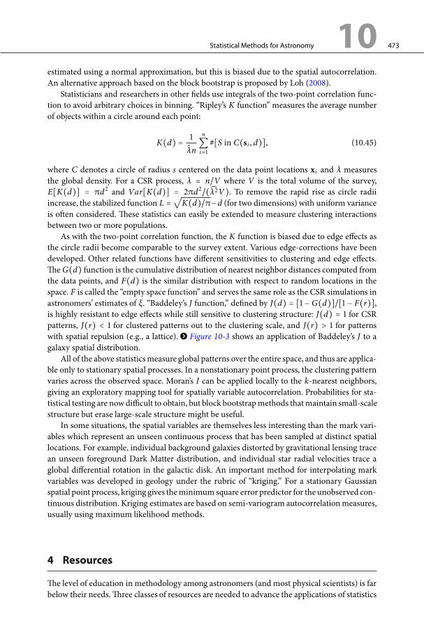
Statistical Methods for Astronomy 10 473
estimated using a normal approximation, but this is biased due to the spatial autocorrelation.An alternative approach based on the block bootstrap is proposed by Loh (2008).
Statisticians and researchers in other fields use integrals of the two-point correlation func-tion to avoid arbitrary choices in binning. “Ripley’s K function” measures the average numberof objects within a circle around each point:
K(d) =λn
n∑
i=#[S in C(si , d)], (10.45)
where C denotes a circle of radius s centered on the data point locations xi and λ measuresthe global density. For a CSR process, λ = n/V where V is the total volume of the survey,E[K(d)] = πd and Var[K(d)] = πd
/(
λV). To remove the rapid rise as circle radiiincrease, the stabilized function L =
√
K(d)/π−d (for two dimensions) with uniform varianceis often considered. These statistics can easily be extended to measure clustering interactionsbetween two or more populations.
As with the two-point correlation function, the K function is biased due to edge effects asthe circle radii become comparable to the survey extent. Various edge-corrections have beendeveloped. Other related functions have different sensitivities to clustering and edge effects.TheG(d) function is the cumulative distribution of nearest neighbor distances computed fromthe data points, and F(d) is the similar distribution with respect to random locations in thespace. F is called the “empty space function” and serves the same role as the CSR simulations inastronomers’ estimates of ξ. “Baddeley’s J function,” defined by J(d) = [ − G(d)]/[ − F(r)],is highly resistant to edge effects while still sensitive to clustering structure: J(d) = for CSRpatterns, J(r) < for clustered patterns out to the clustering scale, and J(r) > for patternswith spatial repulsion (e.g., a lattice). > Figure 10-3 shows an application of Baddeley’s J to agalaxy spatial distribution.
All of the above statisticsmeasure global patterns over the entire space, and thus are applica-ble only to stationary spatial processes. In a nonstationary point process, the clustering patternvaries across the observed space. Moran’s I can be applied locally to the k-nearest neighbors,giving an exploratory mapping tool for spatially variable autocorrelation. Probabilities for sta-tistical testing are nowdifficult to obtain, but block bootstrapmethods thatmaintain small-scalestructure but erase large-scale structure might be useful.
In some situations, the spatial variables are themselves less interesting than the mark vari-ables which represent an unseen continuous process that has been sampled at distinct spatiallocations. For example, individual background galaxies distorted by gravitational lensing tracean unseen foreground Dark Matter distribution, and individual star radial velocities trace aglobal differential rotation in the galactic disk. An important method for interpolating markvariables was developed in geology under the rubric of “kriging.” For a stationary Gaussianspatial point process, kriging gives theminimumsquare error predictor for the unobserved con-tinuous distribution. Kriging estimates are based on semi-variogram autocorrelationmeasures,usually using maximum likelihood methods.
4 Resources
The level of education in methodology among astronomers (and most physical scientists) is farbelow their needs.Three classes of resources are needed to advance the applications of statistics

474 10 Statistical Methods for Astronomy
0
5
10
15
20
25
30
0.00 0.10 0.20 0.30
0.6
0.7
0.8
0.9
1.0
r (degrees)
J(r)
kmhanrstheo
⊡ Fig. 10-3Analysis of a small galaxy redshift survey as a spatial point process using CRAN’s spatstat package.Left: Sky locations of the galaxies with circle sizes scaled to their redshifts, superposed on a kerneldensity estimator of the sky positions. Right: Baddeley’s J function derived from this galaxy sam-ple. J is related to the integral of the two-point correlation function, and is shown with three edgecorrections
for astronomical research: education in existing methodology, research in forefront astrostatis-tics, and advanced statistical software. In the USA, most astronomy students take no classes instatistics while the situation is somewhat better in some other countries. Brief summer schoolsexposing students to methodology are becoming popular, and partially alleviate the educationgap.
Self-education in statistics is quite feasible asmany texts are available and astronomers havethe requisite mathematical background for intermediate-level texts. The Wikipedia Web site isquite effective in presenting material on statistical topics in a compact format. But astronomersconfronting a class of statistical problems would greatly benefit from reading appropriatetextbooks and monographs. Recommended volumes are listed in >Table 10-1.
Research in astrostatistics has rapidly increased since the mid-1990s. Dozens of studiesto treat problems in unevenly spaced time series, survey truncation, faint source detection,fluctuations in the cosmic background radiation, and other issues have been published in theastronomical literature. Some of these efforts develop important new capabilities for astronom-ical data analysis. However, many papers are not conversant with the literature in statistics andother applied fields, even at the level of standard textbooks. Redundant or inadequate treatmentsare not uncommon.
The paucity of software within the astronomical community has, until recently, been a seri-ous hurdle to the implementation of advanced statistical methodology. For decades, advancedmethods were provided only by proprietary statistical software packages like SAS and S-Plus

Statistical Methods for Astronomy 10 475
which the astronomical community did not purchase. The commonly purchased IDL packagefor data analysis and visualization incorporates some statistical methods, particularly those inNumerical Recipes (Press et al. 1986), but not a full scope of modern methods.
The software situation has enormously improved in the past few years with the growthof R, an implementation of the S language released under GNU Public License. R is similarto IDL in style and operation, with brief user commands to implement both simple and com-plex functions and graphics. Base R implements some dozens of standard statistical methods,while its user-supplied add-on packages in the Comprehensive R Archive Network (CRAN)provide thousands of additional functionalities. Together, R/CRAN is a superb new resourcefor promulgation of advanced statistical methods into the astronomical community. Its use isillustrated below. Dozens of books have recently emerged on use of R for various purposes.
4.1 Web Sites and Books
The field of statistics is too vast to be summarized in any single volume or Web site.Wikipediacovers many topics, often in an authoritative fashion (see http://en.wikipedia.org/wiki/List_of_statistics_articles). Additional on-line resources specifically oriented toward astrostatis-tics are provided by Penn State’s Center for Astrostatistics (http://astrostatistics.psu.edu),the California-Harvard Astrostatistics Collaboration (http://www.ics.uci.edu/~dvd/astrostat.html), and the International Computational AstroStatistics Group (http://www.incagroup.org). The International Statistics Institute has formed a new Astrostatistics Network to fostercross-disciplinary interaction (http://isi-web.org/com/ast).
The greatest resource are the hundreds of volumes written by statisticians and applicationexperts. > Table 10-1 gives a selection of these books recommended for astronomers. Theyinclude undergraduate to graduate level texts, authoritativemonographs, and application guidesfor the R software system.
4.2 The R Statistical Software System
R (R Development Core Team 2010) is a high-level software language in the public domainwith C-like syntax. It provides broad capabilities for general data manipulation with extensivegraphics, but its strength is the dozens of built-in statistical functionalities. Compiled code forR can be downloaded for Windows, MacOS, and Unix operating systems from http://r-project.org. The user community of R is estimated to be one to two million individuals, and over 100books have been published to guide researchers in its use.
The Comprehensive R Archive Network (CRAN) of user-supplied add-on packages hasbeen growing nearly exponentially for a decade, currently with ∼3,000 packages. Some CRANpackages have narrow scope, while others are themselves large statistical analysis systemsfor specialized analyses in biology, ecology, econometrics, geography, engineering, and otherresearch communities. CRAN packages, as well as user-provided code in other languages(C, C++, Fortran, Python, Ruby, Perl, Bugs, and XLisp), can be dynamically brought into anR session. Some CRAN packages can be productively used in astronomical science analysis.At the time of writing, only one package has been specifically written for astronomy: CRAN’sfitsio package for input of FITS (Flexible Image Transport System, http://fits.gsfc.nasa.gov/)formatted data used throughout the astronomical community.

476 10 Statistical Methods for Astronomy
The R scripts below, and accompanying figures, illustrate the analysis and graphical outputfrom R and CRAN programs based on an astronomical dataset. Similar R scripts for a widevariety of statistical procedures applied to astronomical datasets are given in Feigelson and Babu(2012).
The first R script inputs a multivariate dataset of photometric and other measurements inASCII using R’s read.table function. The data are extracted from the Sloan Digital Sky Sur-vey quasar survey (Schneider et al. 2010). The dim (dimension) function tells us there are 17columns for 33,845 quasars, names give the column headings, and summary gives the mini-mum, quartiles, mean, and maximum value for each variable. The next lines select the first 200quasars and define redshift and r − i color index variables.
The second script makes a boxplot summarizing the redshift distribution (> Fig. 10-1). Itgives the median with a horizontal line, 25% and 75% quartiles with “hinges,” “whiskers,” out-liers, and notches representing a nonparametric version of the standard deviation. It shows anasymmetrical distribution with a heavy tail toward higher redshifts around z ≃ − . This isone of the common plots made within R.
The third script calculates a sophisticated, computationally intensive, nonparametric kernelsmoother to the two-dimensional distribution of the r− i color index dependence on redshift z.This calculation is provided by theCRAN package np,Nonparametric kernel methods for mixeddatatypes (Hayfield andRacine 2008). Its npregbw function computes an adaptive kernel densityestimator for a p-dimensional matrix of continuous, discrete, and/or categorical variables. Theoptions chosen here give a local-linear regression estimator with a k-nearest neighbor adaptivebandwidth obtained using least-squares cross-validation.>Figure 10-2 shows the quasar color-redshift data points superposed on the kernel smoother with error bars representing the 95%confidence band based on bootstrap resampling. The methods are outlined in the CRAN helpfile and are described in detail by Hall et al. (2007).
# 1. Construct a sample of 200 SDSS quasar redshifts and r-icolors
qso <- read.table(’http://astrostatistics.psu.edu/datasets/SDSS_QSO.dat’, header=T)
dim(qso)names(qso)summary(qso)z_200 <- qso[1:200,4]r_i_200 <- qso[1:200,9] - qso[1:200,11]
# 2. Univariate distribution of redshifts: boxplot
boxplot(z_200, varwidth=T, notch=T, main=’SDSS quasars’,ylab=’Redshift’, pars=list (boxwex=0.3,boxlwd=1.5,whisklwd=1.5,staplelwd=1.5,outlwd=1.5,font=2))
# 3. Bivariate adaptive kernel estimator with bootstrap errors
install.packages(’np’)library(np)

Statistical Methods for Astronomy 10 477
citation(’np’)bw_adap <- npregbw(z_200, r_i_200, regtype=’ll’,bwtype=’adaptive_nn’)npplot(bw_adap, plot.errors.method="bootstrap")points(z_200, r_i_200, pch=20)
To illustrate an analysis of galaxy clustering, the fourth R script inputs 4,215 galaxies froma redshift survey of the Shapley supercluster by Drinkwater et al. (2004). A subsample of 286galaxies is selected from the original sample by specifying a small location in the sky.
The fifth R script starts by installing theCRAN spatstat, Spatial Statistics, package describedby Baddeley (2010). The functions owin and as.ppp convert the data table into a special formatused by spatstat. The galaxies are then plotted on a smoothed spatial distribution with symbolsizes scales to the recessional velocity as a “mark” variable. The second-order J function, cal-culated by the function Jest, is then plotted showing sensitivity at large angles to different edgecorrection algorithms (> Fig. 10-3). The horizontal line is the predictor for “complete spatialrandomness.” Baddeley’s J function is related to Ripley’s K function, the cumulative (unbinned)two-point correlation function, and is designed to reduce edge effects.
# 4. Input and examine Shapley galaxy dataset
shap <- read.table(’http://astrostatistics.psu.edu/datasets/Shapley_galaxy.dat’, header=T)
attach(shap)dim(shap)summary(shap)shap_lo <- shap[(R.A.<214) & (R.A.>209) & (Dec.>-34) &
(Dec.<-27),]dim(shap_lo)
# 5. Display galaxy distribution and calculate BaddeleyJ function
# using spatstat package
install.packages(’spatstat’)library(spatstat)citation(spatstat)shap_lo_win <- owin(range(shap_lo[,1]), range(shap_lo[,2]))shap_lo_ppp <- as.ppp(shap_lo[,c(1,2,4)], shap_lo_win)summary(shap_lo_ppp)
par(mfrow=c(1,2))plot(density(shap_lo_ppp, 0.3), col=gray(5:20/20), main=’’)plot(shap_lo_ppp, lwd=2, add=T)plot(Jest(shap_lo_ppp), lwd=2, col=’black’, cex.lab=1.3,
cex.axis=1.3, main=’’,xlab=’r (degrees)’,legendpos=’topright’)
par(mfrow=c(1,1))

478 10 Statistical Methods for Astronomy
Acknowledgments
Thework of Penn State’s Center for Astrostatistics is supported by NSF grant SSE AST-1047586.
References
Adler, J. 2010, R in a Nutshell: A Desktop QuickReference (O’Reilly Media)
Babu, G. J. 1984, Bootstrapping statistics with lin-ear combinations of chi-squares as weak limit,Sankhya, Ser A, 46, 85–93
Babu, G. J., & Singh, K. 1983, Inference on meansusing the bootstrap, Ann Stat, 11, 999–1003
Babu, G. J., & Singh, K. 1984, On one term Edgeworthcorrection by Efron’s bootstrap, Sankhya, Ser A,46, 219–232
Baddeley, A. 2010, Analysing Spatial Point Patternsin R, http://www.spatstat.org
Bevington, P. R. 1969, Data Reduction andError Analysis for the Physical Sciences(McGraw-Hill)
Bivand, R. S., Pebesma, E. J., & Gómez-Rubio, V.2008, Applied Spatial Data Analysis with R(New York: Springer)
Bowman, A. W., & Azzalini, A. 1997, AppliedSmoothing Techniques for Data Analysis(Clarendon)
Brown, L. D., Cai, T. T., & DasGupta, A. 2001, Inter-val estimation for a binomial proportion (withdiscussion), Stat Sci, 16, 101–133
Chatfield, C. 2004, The Analysis of Time Series: AnIntroduction (6th ed.; London: Chapman andHall)
Chen, C.-h., Härdle, W., & Unwin, A. (eds.), 2008,Handbook of Data Visualization (New York:Springer)
Conover, W. J. 1999, Practical Nonparametric Statis-tics (New York: Wiley)
Cowan, G. 2006, The small-N problem in high energyphysics, in Statistical Challenges in ModernAstronomy IV, ed. G. J. Babu, & E. D. Feigelson(New York: Springer), 75–86
Cowpertwait, P. S. P., & Metcalfe, A. V. 2009, Intro-ductory Time Series with R (New York: Springer)
Cox, D. R. 2006, Principles of Statistical Inference(Cambridge, UK: Cambridge University Press)
Dalgaard, P. 2008, Introductory Statistics with R(New York: Springer)
Dempster, A. P., Laird, N. M., & Rubin, D. B. 1977,Maximum likelihood from incomplete data viathe EM algorithm, J R Stat Soc B, 39, 1–38
Drinkwater, M. J., Parker, Q. A., Proust, D. Slezak,E., & Quintana, H., 2004, Publ Astron Soc Aust,21, 89
Duda, R. O., Hart, P. E., & Stork, D. G. 2001, PatternClassification (2nd ed.; New York: Wiley)
Edelson, R. A., & Krolik, J. H. 1988, The discrete cor-relation function: A new method for analyzingunevenly sampled variability data, Astrophys J333, 646–659
Efron, B., & Tibshirani, R. J. 1993, An Introductionto the Bootstrap (London: Chapman and Hall)
Evans, M., Hastings, N., & Peacock, B. 2000, Statisti-cal Distributions (3rd ed.; New York: Wiley)
Everitt, B. S., Landau, S., & Leese, M. 2001, ClusterAnalysis (4th ed.; Arnold)
Feigelson, E. D., & Babu, G. J. 2012, Modern Statisti-cal Methods for Astronomy with R Applications(Cambridge, UK: Cambridge University Press)
Feigelson, E. D., & Nelson, P. I. 1985, Statisticalmethods for astronomical data with upper limits.I – Univariate distributions, Astrophys J 293,192–206
Fortin, M.-J., & Dale, M. R. T. 2005, Spatial Anal-ysis: A Guide for Ecologists (Cambridge, UK:Cambridge University Press)
Fisher, R. A. 1922, On the mathematical foundationsof theoretical statistics, Philos Trans R Soc A,222, 309–368
Gelman, A., Carlin, J. B., Stern, H. S., & Rubin, D. B.2004, Bayesian Data Analysis (2nd ed.; London:Chapman and Hall)
Gregory, P. C. 2005, Bayesian Logical Data Anal-ysis for the Physical Sciences: A Compara-tive Approach with Mathematica Support (Cam-bridge, UK: Cambridge University Press)
Hall, P., Li, Q., & Racine, J. S. 2007, Nonparametricestimation of regression functions in the pres-ence of irrelevant regressors, Rev Econ Stat, 89,784–789
Hastie, T., Tibshirani, R., & Friedman, J. 2009, TheElements of Statistical Learning: Data Mining,Inference, and Prediction (2nd ed.; New York:Springer)
Hayfield, T., & Racine, J. S. 2008, NonparametricEconometrics: The np Package, J Stat Softw,27(5), 1–32

Statistical Methods for Astronomy 10 479
Helsel, D. R. 2004, Nondetects and Data Analy-sis: Statistics for Censored Environmental Data(Wiley-Interscience)
Hogg, R. V., & Tanis, E. 2009, Probability and Statis-tical Inference (10th ed.; Prentice Hall)
Hou, A., Parker, L. C., Harris, W. E., & Wilman,D. J. 2009, Statistical tools for classifying galaxygroup dynamics, Astrophys J, 702, 1199–1210
Illian, J., Penttinen, A., Stoyan, H., & Stoyan, D.2008, Statistical Analysis and Modeling of Spa-tial Point Processes (Wiley-Interscience)
James, F. 2006, Statistical Methods in ExperimentalPhysics (2nd ed.; World Scientific)
Johnson, N. L., Kotz, S., & Balakrishnan, N. 1994,Continuous Univariate Distributions, Vols. 1and 2 (2nd ed.; Wiley-Interscience)
Johnson, R. A., & Wichern, D. W. 2007, Applied Mul-tivariate Statistical Analysis (6th ed.; Prentice-Hall)
Kashyap, V. L., van Dyk, D. A., Connors, A., Freeman,P. E., Siemiginowska, A., Xu, J., & Zezas, A. 2010,On computing upper limits to source intensities,Astrophys J, 719, 900–914
Kelly, B. C. 2007, Some aspects of measurement errorin linear regression of astronomical data, Astro-phys J, 665, 1489–1506
Kitagawa, G., & Gersch, W. 1996, Smoothness PriorsAnalysis of Time Series (New York: Springer)
Klein, J. P., & Moeschberger, M. L. 2010, SurvivalAnalysis: Techniques for Censored and Trun-cated Data (New York: Springer)
Kruschke, J. K. 2011, Doing Bayesian Data Analysis:A Tutorial with R and BUGS (Academic)
Kutner, M. H., Nachtsheim, C. J., & Neter, J. 2004,Applied Linear Regression Models (4th ed.;McGraw-Hill)
Lawless, J. F. 2002, Statistical Models and Methodsfor Lifetime Data (2nd ed.; New York: Wiley)
Lilliefors, H. W. 1969, On the Kolmogorov-Smirnovtest for the exponential distribution with meanunknown, J Am Stat Assoc, 64, 387–389
Loh, J. M. 2008, A valid and fast spatial bootstrap forcorrelation functions, Astrophys J, 681, 726–734
Lucy, L. B. 1974, An iterative technique for the rec-tification of observed distributions, Astron J, 79,745–754
Lupton, R. 1993, Statistics in Theory and Practice(Princeton University Press)
Maindonald, J., & Braun, W. J. 2010, Data Analy-sis and Graphics Using R: An Example-BasedApproach (3rd ed.; Cambridge, UK: CambridgeUniversity Press)
Marquardt, D. W., & Acuff, S. K. 1984, Directquadratic spectrum estimation with irregularly
spaced data, in Time Series Analysis of Irregu-larly Observed Data, ed. E. Parzen, Lecture Notesin Statistics, Vol. 25 (New York: Springer)
Martínez, V. J., & Saar, E. 2002, Statistics of theGalaxy Distribution (London: Chapman andHall)
McLachlan, G. J., & Krishnan, T. 2008, The EMAlgorithm and Extensions (2nd ed.; Wiley-Interscience)
Miller, C. J., Nichol, R. C., Genovese, C., &Wasserman, L. 2002, A nonparametric analy-sis of the cosmic microwave background powerspectrum, Astrophys J, 565, L67–L70
Nason, G. 2008, Wavelet Methods in Statistics with R(New York: Springer)
Park, T., Kashyap, V. L., Siemiginowska, A., van Dyk,D. A., Zezas, A., Heinke, C., & Wargelin, B.J. 2006, Bayesian estimation of hardness ratios:Modeling and computations, Astrophys J, 652,610–628
Percival, D.B., & Walden, A.T. 1993, Spectral Anal-ysis for Physical Applications (Cambridge, UK:Cambridge University Press)
Press, W. H., Teukolsky, S. A., Vetterling, W. T., &Flannery, B. P. 1986, Numerical Recipes: TheArt of Scientific Computing (Cambridge, UK:Cambridge University Press)
Protassov, R., van Dyk, D. A., Connors, A., Kashyap,V. L., & Siemiginowska, A. 2002, Statistics, han-dle with care: Detecting multiple model compo-nents with the likelihood ratio test, Astrophys J,571, 545–559
R Development Core Team 2010, R: A Language andEnvironment for Statistical Computing (Vienna:R Foundation for Statistical Computing)
Rao, C. R. 1997, Statistics and Truth: Putting Chanceto Work (2nd ed.; World Scientific)
Reegen, P. 2007, SigSpec. I. Frequency- and phase-resolved significance in Fourier space, AstronAstrophys, 467, 1353–1371
Rice, J. 1994, Mathematical Statistics and Data Anal-ysis (2nd ed.; Duxbury Press)
Ross, S. M. 2010, A First Course in Probability (10thed.; Prentice Hall)
Sarkar, D. 2008, Lattice: Multivariate Data Visualiza-tion with R (New York: Springer)
Scargle, J. D. 1982, Studies in astronomical timeseries analysis. II: Statistical aspects of spectralanalysis of unevenly spaced data, Astrophys J263, 835–853
Schneider, D. P. et al. 2010, The Sloan Digital SkySurvey Quasar Catalog. V. Seventh Data Release,Astron J, 139, 2360–2373
Shumway, R. H., & Stoffer, D. S., 2006, Time SeriesAnalysis and Its Applications with R Examples(2nd ed.; New York: Springer)

480 10 Statistical Methods for Astronomy
Silverman, B. W. 1998, Density Estimation (London:Chapman and Hall)
Simonetti, J. H., Cordes, J. M., & Heeschen, D. S.1986, Flicker of extragalactic radio sources attwo frequencies, Astrophys J 296, 46–59
Spergel, D. N., Verde, L., Peiris, H. V., Komatsu, E.,Nolta, M. R., Bennett, C. L., Halpern, M.,Hinshaw, G., Jarosik, N., Kogut, A., Limon, M.,Meyer, S. S., Page, L., Tucker, G. S., Wei-land, J. L., Wollack, E., & Wright, E. L. 2003,First-year Wilkinson Microwave AnisotropyProbe (WMAP) observations: Determinationof cosmological parameters, Astrophys J, 148,175–194
Starck, J.-L., & Murtagh, F. 2006, Astronomical Imageand Data Analysis (2nd ed.; New York: Springer)
Stigler, S. M. 1986, The History of Statistics:The Measurement of Uncertainty Before 1900(Harvard University Press)
Takezawa, K. 2005, Introduction to NonparametricRegression (New York: Wiley)
Wang, X., Woodroofe, M., Walker, M. G., Mateo,M., & Olszewski, E. 2005, Estimating Dark Mat-ter distributions, Astrophys J, 626, 45–158
Way, M. J., Scargle, J. D., Ali, K., & Srivastava, A. N.(eds.), 2011, Advances in Machine Learning andData Mining for Astronomy (London: Chapmanand & Hall)
Wasserman, L. 2005, All of Statistics: A Con-cise Course in Statistical Inference (New York:Springer)
Wickham, H. 2009, ggplot2: Elegant Graphics forData Analysis (2nd ed.; New York: Springer)
Zoubir, A. M., & Iskander, D. R. 2004, BootstrapTechniques for Signal Processing, (Cambridge,UK: Cambridge University Press)