10. assembly language, models of computation · pdf file• main elements: – values...

6.004 Computation Structures L10: Assembly Language, Models of Computation, Slide #1

10. Assembly Language, Models of Computation

6.004x Computation Structures Part 2 – Computer Architecture

Copyright © 2015 MIT EECS


Beta ISA Summary

•  Storage: –  Processor: 32 registers (r31 hardwired to 0) and PC

–  Main memory: Up to 4 GB, 32-bit words, 32-bit byte addresses, 4-byte-aligned accesses

•  Instruction formats:

•  Instruction classes: –  ALU: Two input registers, or register and constant

–  Loads and stores: access memory

–  Branches, Jumps: change program counter

OPCODE rc ra rb unused

OPCODE rc ra 16-bit signed constant

32 bits


Programming Languages

Means, to the BETA, Reg[4]ßReg[2]+Reg[3]

opcode rb ra

1 0

(unused)

0 0 0 1 0 0 0 0 1 0 0 0 0 1 0 0 0 1

rc

0 0 0 0 0 0 0 0 0 0 0

32-bit (4-byte) ADD instruction:

We’d rather write in assembly language:

ADD(R2,R3,R4)

a=b+c;

or better yet a high-level language:

0

Today

Coming up


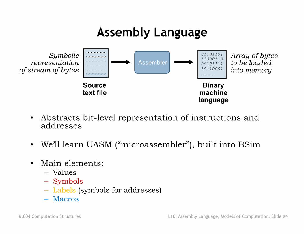
•  Abstracts bit-level representation of instructions and addresses

•  We’ll learn UASM (“microassembler”), built into BSim

•  Main elements: –  Values –  Symbols –  Labels (symbols for addresses) –  Macros

Assembler 01101101 11000110 00101111 10110001 .....

Source text file

Binary machine language

Array of bytes to be loaded into memory

Assembly Language

Symbolic representation

of stream of bytes


Example UASM Source File

•  Comments after //, ignored by assembler (also /*…*/) •  Symbols are symbolic representations of a constant

value (they are NOT variables!)

•  Labels are symbols for addresses •  Macros expand into sequences of bytes

–  Most frequently, macros are instructions

–  We can use them for other purposes

N=12//loopindexinitialvalueADDC(r31,N,r1) //r1=loopindexADDC(r31,1,r0) //r0=accumulatedproduct

loop:MUL(r0,r1,r0) //r0=r0*r1SUBC(r1,1,r1) /*r1=r1–1*/BNE(r1,loop,r31) //ifr1!=0,NextPC=loop


How Does It Get Assembled?

•  Load predefined symbols into a symbol table

•  Read input line by line –  Add symbols to symbol table

as they are defined –  Expand macros, translating

symbols to values first

Text input N=12ADDC(r31,N,r1)ADDC(r31,1,r0)

loop:MUL(r0,r1,r0)SUBC(r1,1,r1)BNE(r1,loop,r31)

Binary output Symbol Value

r0 0

r1 1

r31 31

Symbol table

N 12

11000000001111110000000000001100[0x00]11000000000111110000000000000001[0x04]10001000000000000000100000000000[0x08]

loop 8

……


Registers are Predefined Symbols

•  r0 = 0, …, r31 = 31 •  Treated like

normal symbols:

•  No “type checking” if you use the wrong opcode…

ADDC(r31,N,r1)

ADDC(31,12,1)

11000000001111110000000000001100

Substitute symbols with their values

Expand macro

ADDC(r31,r12,r1)

ADDC(31,12,1)

Reg[1]ßReg[31]+12

ADD(r31,N,r1)

ADD(31,12,1)

Reg[1]ßReg[31]+Reg[12]


Labels and Offsets

•  Label value is the address of a memory location

•  BEQ/BNE macros compute offset automatically

•  Labels hide addresses!

Input file N=12ADDC(r31,N,r1)ADDC(r31,1,r0)


Symbol Value

r0 0

r1 1

r31 31

Symbol table

11000000001111110000000000001100[0x00]11000000000111110000000000000001[0x04]10001000000000010000000000000000[0x08]11000100001000010000000000000001[0x0C]01110111111000011111111111111101[0x10] N 12

loop 8

Output file

offset=(label-<addrofBNE/BEQ>)/4–1=(8–16)/4–1=-3

…


Mighty Macroinstructions

// Macro to generate 4 consecutive bytes: .macro consec(n) n n+1 n+2 n+3

// Invocation of above macro: consec(37)

Macros are parameterized abbreviations, or shorthand

⇒ 37 37+1 37+2 37+3 ⇒ 37 38 39 40 Is expanded to

// Assemble into bytes, little-endian: .macro WORD(x) x%256 (x/256)%256 .macro LONG(x) WORD(x) WORD(x >> 16)

Here are macros for breaking multi-byte data types into byte-sized chunks

Has same effect as:

0xef 0xbe 0xad 0xde Mem: 0x100 0x101 0x102 0x103

. = 0x100 LONG(0xdeadbeef) Boy, that’s hard to read.

Maybe, those big-endian types do have a point.


Assembly of Instructions

// Assemble Beta op instructions .macro betaop(OP,RA,RB,RC) { .align 4 LONG((OP<<26)+((RC%32)<<21)+((RA%32)<<16)+((RB%32)<<11)) }

OPCODE RC RA RB UNUSED

OPCODE RC RA 16-BIT SIGNED CONSTANT

110000 ADDC = 0x30 = 1000000000000000 -32768 = 01111 15 = 00000 0 =

1000000000000000 00000 01111 110000 “.align 4” ensures instructions will begin on word boundary (i.e., address = 0 mod 4)

For example: .macro ADDC(RA,C,RC) betaopc(0x30,RA,C,RC)

ADDC(R15, -32768, R0) --> betaopc(0x30,15,-32768,0)

// Assemble Beta opc instructions .macro betaopc(OP,RA,CC,RC) { .align 4 LONG((OP<<26)+((RC%32)<<21)+((RA%32)<<16)+(CC % 0x10000)) } // Assemble Beta branch instructions .macro betabr(OP,RA,RC,LABEL) betaopc(OP,RA,((LABEL-(.+4))>>2),RC)


Example Assembly ADDC(R3,1234,R17)

betaopc(0x30,R3,1234,R17)

expand ADDC macro with RA=R3, C=1234, RC=R17

.align 4 LONG((0x30<<26)+((R17%32)<<21)+((R3%32)<<16)+(1234 % 0x10000))

expand betaopc macro with OP=0x30, RA=R3, CC=1234, RC=R17

WORD(0xC22304D2) WORD(0xC22304D2 >> 16)

expand LONG macro with X=0xC22304D2

0xC22304D2%256 (0xC22304D2/256)%256 WORD(0xC223)

expand first WORD macro with X=0xC22304D2

0xD2 0x04 0xC223%256 (0xC223/256)%256

evaluate expressions, expand second WORD macro with X=0xC223

0xD2 0x04 0x23 0xC2

evaluate expressions


UASM Macros for Beta Instructions

| BETA Instructions: .macro ADD(RA,RB,RC) betaop(0x20,RA,RB,RC) .macro ADDC(RA,C,RC) betaopc(0x30,RA,C,RC) .macro AND(RA,RB,RC) betaop(0x28,RA,RB,RC) .macro ANDC(RA,C,RC) betaopc(0x38,RA,C,RC) .macro MUL(RA,RB,RC) betaop(0x22,RA,RB,RC) .macro MULC(RA,C,RC) betaopc(0x32,RA,C,RC)

• •

• .macro LD(RA,CC,RC) betaopc(0x18,RA,CC,RC) .macro LD(CC,RC) betaopc(0x18,R31,CC,RC) .macro ST(RC,CC,RA) betaopc(0x19,RA,CC,RC) .macro ST(RC,CC) betaopc(0x19,R31,CC,RC)

• •

• .macro BEQ(RA,LABEL,RC) betabr(0x1C,RA,RC,LABEL) .macro BEQ(RA,LABEL) betabr(0x1C,RA,r31,LABEL) .macro BNE(RA,LABEL,RC) betabr(0x1D,RA,RC,LABEL) .macro BNE(RA,LABEL) betabr(0x1D,RA,r31,LABEL)

Convenience macros so we don’t have to specify R31…

(defined in beta.uasm)


Pseudoinstructions •  Convenience macros that expand to one or more real instructions •  Extend set of operations without adding instructions to the ISA

//Conveniencemacrossowedon’thavetouseR31.macroLD(CC,RC) LD(R31,CC,RC).macroST(RA,CC) ST(RA,CC,R31).macroBEQ(RA,LABEL) BEQ(RA,LABEL,R31).macroBNE(RA,LABEL) BNE(RA,LABEL,R31).macroMOVE(RA,RC) ADD(RA,R31,RC) //Reg[RC]<-Reg[RA].macroCMOVE(CC,RC) ADDC(R31,C,RC) //Reg[RC]<-C.macroCOM(RA,RC) XORC(RA,-1,RC) //Reg[RC]<-~Reg[RA].macroNEG(RB,RC) SUB(R31,RB,RC) //Reg[RC]<--Reg[RB].macroNOP() ADD(R31,R31,R31) //donothing

.macroBR(LABEL) BEQ(R31,LABEL) //alwaysbranch.macroBR(LABEL,RC) BEQ(R31,LABEL,RC) //alwaysbranch .macroCALL(LABEL) BEQ(R31,LABEL,LP) //callsubroutine.macroBF(RA,LABEL,RC) BEQ(RA,LABEL,RC) //0isfalse.macroBF(RA,LABEL) BEQ(RA,LABEL).macroBT(RA,LABEL,RC) BNE(RA,LABEL,RC) //1istrue.macroBT(RA,LABEL) BNE(RA,LABEL)

//Multi-instructionsequences.macroPUSH(RA) ADDC(SP,4,SP)ST(RA,-4,SP).macroPOP(RA) LD(SP,-4,RA)ADDC(SP,-4,SP)


Factorial with Pseudoinstructions

N=12ADDC(r31,N,r1)ADDC(r31,1,r0)


N=12CMOVE(N,r1)CMOVE(1,r0)

loop:MUL(r0,r1,r0)SUBC(r1,1,r1)BNE(r1,loop)

Before After


Raw Data

•  LONG assembles a 32-bit value –  Variables

–  Constants > 16 bits

N: LONG(12)factN:LONG(0xdeadbeef)

…Start:

LD(N,r1)CMOVE(1,r0)

loop:MUL(r0,r1,r0)SUBC(r1,1,r1)BT(r1,loop)ST(r0,factN)

Symbol Value

N 0

factN 4

Symbol table

…

LD(r31,N,r1)

LD(31,0,1)

Reg[1]ßMem[Reg[31]+0]ßMem[0]ß12


UASM Expressions and Layout

•  Values can be written as expressions –  Assembler evaluates expressions, they are not translated to

instructions to compute the value!

•  The “.” (period) symbol means the next byte address to be filled –  Can read or write to it –  Useful to control data layout or leave empty space (e.g., for

arrays)

.=0x100 //Assembleinto0x100LONG(0xdeadbeef)k=. //Symbol“k”hasvalue0x104LONG(0x00dec0de).=.+16 //Skip16bytesLONG(0xc0ffeeee)

A=7+3*0x0cc41B=A-3


Summary: Assembly Language

•  Low-level language, symbolic representation of sequence of bytes. Abstracts: –  Bit-level representation of instructions

–  Addresses

•  Elements: Values, symbols, labels, macros •  Values can be constants or expressions

•  Symbols are symbolic representations of values •  Labels are symbols for addresses

•  Macros are expanded to byte sequences: –  Instructions

–  Pseudoinstructions (translate to 1+ real instructions)

–  Raw data

•  Can control where to assemble with “.” symbol


Universality?

•  Recall: We say a set of Boolean gates is universal if we can implement any Boolean function using only gates from that set.

•  What problems can we solve with a von Neumann

computer? (e.g., the Beta) –  Everything that FSMs can solve?

–  Every problem? –  Does it depend on the ISA?

•  Needed: a mathematical model of computation –  Prove what can be computed, what can’t


Models of Computation

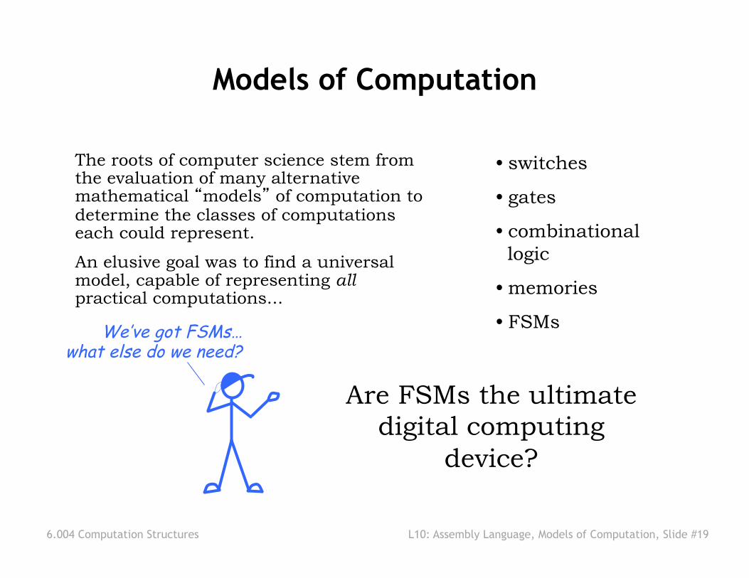
The roots of computer science stem from the evaluation of many alternative mathematical “models” of computation to determine the classes of computations each could represent.

An elusive goal was to find a universal model, capable of representing all practical computations...

• switches

• gates

• combinational logic

• memories

• FSMs

Are FSMs the ultimate digital computing

device?

We’ve got FSMs… what else do we need?


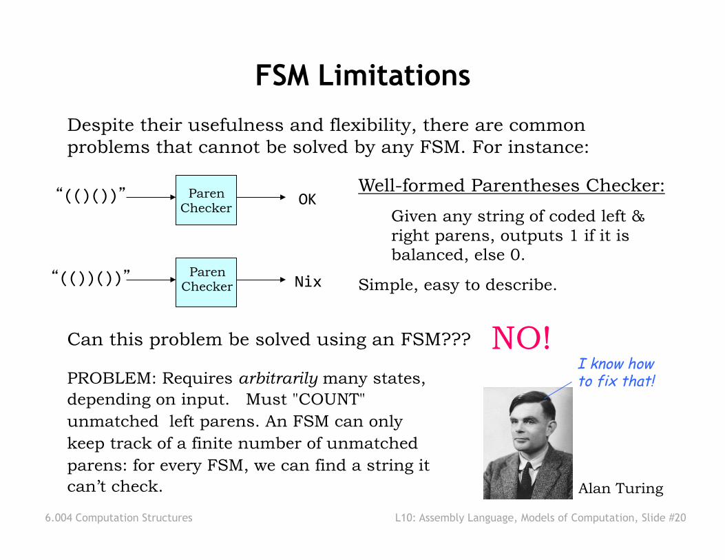
FSM Limitations Despite their usefulness and flexibility, there are common problems that cannot be solved by any FSM. For instance:

Paren Checker

“(()())” OK

Paren Checker

“(())())” Nix

Well-formed Parentheses Checker:

Given any string of coded left & right parens, outputs 1 if it is balanced, else 0.

Simple, easy to describe.

PROBLEM: Requires arbitrarily many states, depending on input. Must "COUNT" unmatched left parens. An FSM can only keep track of a finite number of unmatched parens: for every FSM, we can find a string it can’t check.

NO!

Alan Turing

I know how to fix that!

Can this problem be solved using an FSM???


Turing Machines

Alan Turing was one of a group of researchers studying alternative models of computation. He proposed a conceptual model consisting of an FSM combined with an infinite digital tape that could be read and written at each step. • encode input as symbols on tape • FSM reads tape/writes symbols/ changes state until it halts

• Answer encoded on tape Turing’s model (like others of the time) solves the "FINITE" problem of FSMs.

S1

1 1 1 0 0 0 0 1 0 0 0 0 0 0 0 0

S2

0,(1,R)

0,(1,L)

1,Halt

1,(1,L)

Bounded tape configuration can be expressed as a (large!) integer

FSMs can be enumerated and given a (very large) integer index.

We can talk about TM 347 running on input 51, producing an answer of 42. TMs as integer functions: y = TMI[x]


Other Models of Computation…

Turing Machines [Turing]

FSM i

0 1 1 0 0 0 1 0 0

Alan Turing

Recursive Functions [Kleene] F(0,x) ≡ xF(1+y,x) ≡ 1+F(x,y)

(define (fact n) (... (fact (- n 1)) ...)

Stephen Kleene

Lambda calculus [Church, Curry, Rosser...]

λ x. λ y.xxy

(lambda(x)(lambda(y)(x (x y))))

Alonzo Church

Production Systems [Post, Markov]

α → β IF pulse=0 THEN patient=dead

Emile Post


Computability FACT: Each model studied is capable of computing exactly the same set of integer functions!

Proof Technique: Constructions that translate between models

BIG IDEA:

Computability, independent of computation scheme chosen

Church's Thesis:

Every discrete function computable by ANY realizable machine is computable by some Turing machine.

f(x) computable ⇔ for some k, all x f(x) = Tk[x]

unproved, but universally accepted...


FSM

0 1 1 0 0 0 1 0 0

Multiplication

FSM

0 1 1 0 0 0 1 0 0

Sorting

FSM

0 1 1 0 0 0 1 0 0

Factorization FSM

0 1 1 0 0 0 1 0 0

Primality Test

Is there an alternative to infinitely many ad-hoc Turing Machines?

“special-purpose” Turing Machines....

meanwhile...

Turing machines Galore!


Here’s an interesting function to explore: the Universal function, U, defined by

SURPRISE! U is computable by a Turing Machine:

TU k

j Tk[j]

In fact, there are infinitely many such machines. Each is capable of performing any computation that can be performed by any TM!

U(k, j) = Tk[j]

Could this be computable???

it sure would be neat to have a single, general-purpose machine...

The Universal Function


Universality

TU k

j Tk[j]

What’s going on here?

k encodes a “program” – a description of some arbitrary machine.

j encodes the input data to be used.

TU interprets the program, emulating its processing of the data!

KEY IDEA: Interpretation. Manipulate coded representations of computing machines, rather than the machines themselves.


Turing Universality

The Universal Turing Machine is the paradigm for modern general-purpose computers!

Basic threshold test: Is your computer Turing Universal ? •  If so, it can emulate every other Turing machine! •  Thus, your computer can compute any computable

function

To show your computer is Universal: demonstrate that it can emulate some known UTM.

•  Actually given finite memory, can only emulate UTMs + inputs up to a certain size

•  This is not a high bar: conditional branches (BEQ) and some simple arithmetic (SUB) are enough.


Coded Algorithms: Key to CS data vs hardware

Algorithms as data: enables COMPILERS: analyze, optimize, transform behavior

SOFTWARE ENGINEERING: Composition, iteration, abstraction of coded behavior

F(x) = g(h(x), p((q(x)))

TCOMPILER-X-to-Y[PX] = PY, such that TX[PX, z] = TY[PY, z]

Px

Py

Pgm

Pgm

PLINUX PJade

Pgm Pgm

Pgm

LANGUAGE DESIGN: Separate specification from implementation

•  C, Java, JSIM, Linux, ... all run on X86, Sun, ARM, JVM, CLR, ...

•  Parallel development paths: •  Language/Software design •  Interpreter/Hardware design


Uncomputability (!)

Uncomputable functions: There are well-defined discrete functions that a Turing machine cannot compute

–  No algorithm can compute f(x) for arbitrary x in finite number of steps

–  Not that we don’t know algorithm - can prove no algorithm exists

–  Corollary: Finite memory is not the only limiting factor on whether we can solve a problem

The most famous uncomputable function is the so-called Halting function, fH(k, j), defined by:

fH(k, j) = 1 if Tk[j] halts;

0 otherwise.

fH(k, j) determines whether the kth TM halts when given a tape containing j.


If fH is computable, it is equivalent to some TM (say, TH):

TH

k

j 1 iff Tk[j] halts, else 0

Then TN (N for “Nasty”), which must be computable if TH is:

TN

TH ? 1

0

LOOP

HALT

TN[x]: LOOPS if Tx[x] halts; HALTS if Tx[x] loops

Finally, consider giving N as an argument to TN:

TN[N]: LOOPS if TN[N] halts; HALTS if TN[N] loops

TN can’t be computable, hence TH can’t either!

x

Why fH is Uncomputable

10. assembly language, models of computation · pdf file• main elements: – values...

Documents