1

Welcome toPMBA0608: Economics/Statistics Foundation

Fall 2006Sessions 9 & 10: October 28

Athens

2

I have posted anonymous feedbacks on line at

http://www.marietta.edu/~khorassj/pmba608/cur608.html

3

Discuss Assignment 4: Question 1, Page 110 of Econ

a. Mystery novels have a more elastic demand because they are not required and there are other types of novels available in the market.

b. Beethoven recordings have more elastic demand because they are more narrowly defined than classical music recordings.

4

Question 1, Page 110 of Econ

c) Subway rider’s demand during the next 5 years is more elastic because they have more time to adjust.

d) Root beer has a more elastic demand. It is not a necessity and there are more substitutes for it than for water.

5

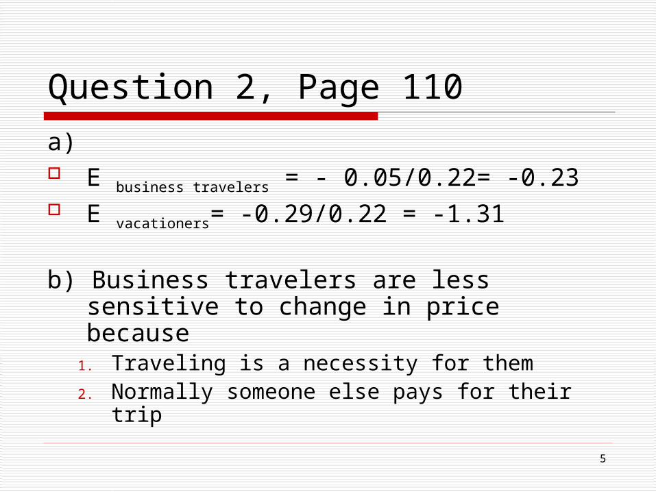
Question 2, Page 110

a) E business travelers = - 0.05/0.22= -0.23 E vacationers= -0.29/0.22 = -1.31

b) Business travelers are less sensitive to change in price because

1. Traveling is a necessity for them2. Normally someone else pays for their

trip

6

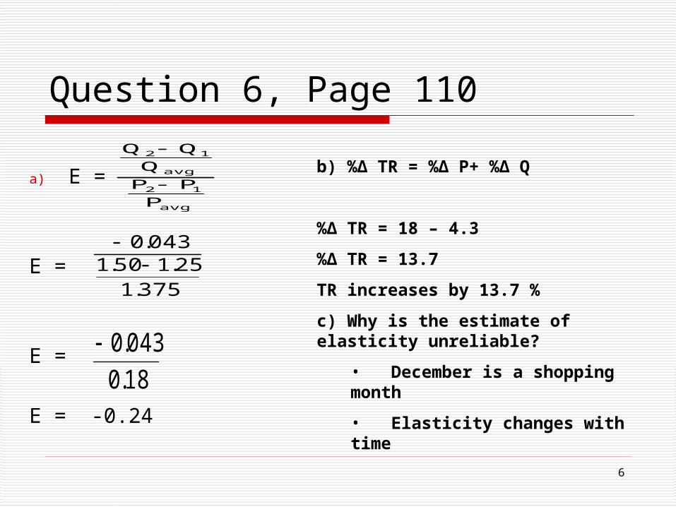
Question 6, Page 110

a) E =

E =

E =

E = -0.24

avg

12

avg

12

PPP

QQQ

375.125.150.1

043.0

18.0

043.0

b) %Δ TR = %Δ P+ %Δ Q

%Δ TR = 18 – 4.3

%Δ TR = 13.7

TR increases by 13.7 %

c) Why is the estimate of elasticity unreliable?

• December is a shopping month

• Elasticity changes with time

7

Question 11 Page 111 (a)

P

Q

Both demands

S resorts

S autos

P1

New demand for both

Q1

P2

resort

P2

auto

O2 autoQ2

resort

8

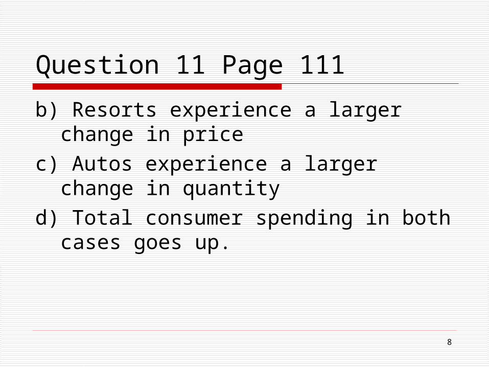
Question 11 Page 111

b) Resorts experience a larger change in price

c) Autos experience a larger change in quantity

d) Total consumer spending in both cases goes up.

9

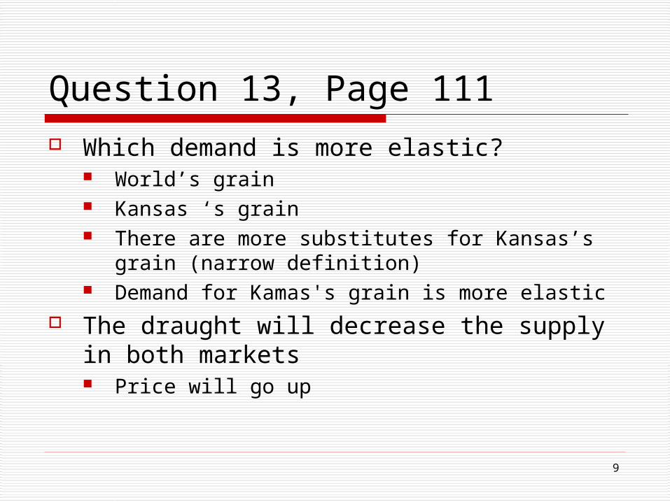
Question 13, Page 111 Which demand is more elastic?

World’s grain Kansas ‘s grain There are more substitutes for Kansas’s grain

(narrow definition) Demand for Kamas's grain is more elastic

The draught will decrease the supply in both markets Price will go up

10

In Kansas loss in revenue > gain in revenue

In World loss in revenue < gain in revenue

S1 (both)

P

Q

Kansas D

World D

P1

Q1

S2 (both)

P2 world

Q2 world

P2 Kansas

Q2 Kansa

s

11

Question 13, Page 111

The demand for world’s grain is inelastic So if P goes up TR goes up

The demand for Kansas ‘s grain is elastic So if P goes up TR goes down.

12

Next Class

Wednesday, November 8, 19:30-22:45 Try to be in Chillicothe Chapter 4 of Stat Chapter 23 of Econ

13

Today

We will start Chapter 4 of Stat Instead of moving to Chapter 23 of

Econ, we will cover Chapter 6 of Econ Reason?

Timely topics

14

Assignment 5: due on or before November 4

1. 4.5, Page 141 of Stat. (Do it using Excel. Show your work and the graph)

2. 4.11,Page 141 of Stat.3. 4.17, Page 142 of Stat. (Do this one

manually using the binomial formula. Show your work.)

4. Problem 2, Page 132 of Econ5. Problem 4, Page 133 of Econ (bonus)

15

Chapter 4 of Stat

When a coin is flipped, the outcome is either a head or a tail. Let’s flip a coin 5 times; what is the probability of getting

3 heads?

when an economist forecasts the inflation rate for next year; she can either be correct or incorrect. Let’s ask 6 economists to forecast the inflation rate;

what is the probability that they are all right?

when a student takes an exam, he will either pass or fail. Let’s have 4 students take the exam; what is the

probability that 2 of them pass the exam?

16

These are examples of binomial experiments

The prefix bi refers to the fact that there are two possible outcomes (e.g., head or tail, correct or incorrect, pass or fail) to each trial in the binomial experiment.

A binomial experiment (and the binomial distribution denoted by B(n,p)) is characterized by two parameters: n, the number of trials which are performed P, the probability of success on a single trial

17

Not all experiments that have two possible outcomes are binomial Properties of a binomial distribution

1. n identical trials 2. all trials are independent 3. each trial has only two mutually exclusive

possible outcomes, success or failure 4. P(success) is constant from trial to trial 5. We are interested in counting the number

of success (x) in the set of n random trials

18

Is this a binomial experiment? What is the probability of obtaining

exactly 3 heads if a fair coin is flipped 6 times? Yes, it meets all 5 conditions

What is the probability of obtaining exactly 3 defected goods if we choose 6 goods and we adjust the machine after each selection? No, condition 4 is not met.

19

Is this a binomial experiment? What is the probability of having to

have 3 children until you have a boy? No, conditions 1 and 5 are not met not

(We are not counting successes in fixed number of trials.)

First part of Exercise 4.1, page 140 No, P (red first ball) is 3/5 P (red second ball) depends on what was

the first ball. Conditions 2 and 4 are not met.

20

Note If the sample size is large relative to

the population size, then the probability of success will not remain constant from trial to trial Example

If 8 students take the exam and you choose 5 of them, P (first student pass) ≠ P (5th student pass)

If 100 students take the exam and you choose 5 of them, P (first student pass) will be closer to P (5th student pass)

21

Rule of thumb

If n/N ≥ 0.5 then the experiment is not binomial Where

n is sample size and N is the population size

22

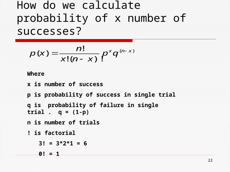
How do we calculate probability of x number of successes?

)(

)!(!

!)( xnxqp

xnx

nxp

Where

x is number of success

p is probability of success in single trial

q is probability of failure in single trial . q = (1-p)

n is number of trials

! is factorial

3! = 3*2*1 = 6

0! = 1

23

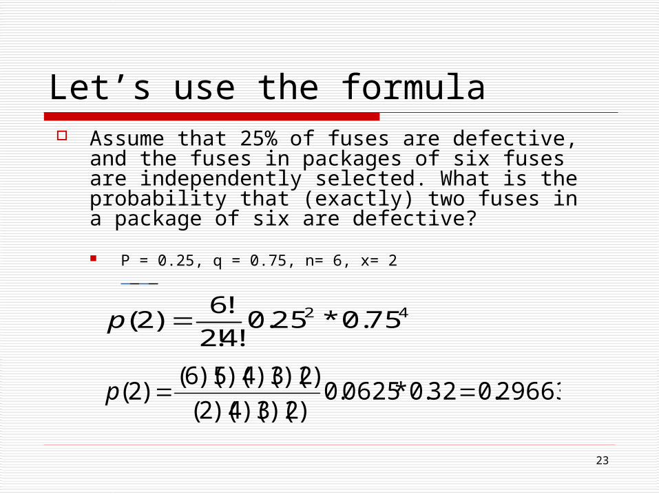
Let’s use the formula Assume that 25% of fuses are defective, and

the fuses in packages of six fuses are independently selected. What is the probability that (exactly) two fuses in a package of six are defective?

P = 0.25, q = 0.75, n= 6, x= 2

42 75.0*25.0!4!2

!6)2( p

29663.032.0*0625.0)2)(3)(4)(2(

)2)(3)(4)(5)(6()2( p

24

Can we calculate probability of x = 0, x=1, x=3, x=4, x=5, x=6? P (0) =0.17798 P (1) =0.35596 P (2) = 0.29663 P (3)= 0.13184 P (4) =0.03296 P (5) =0.00439 P (6) =0.00024 Do these probability have to add up to 1? Yes, they cover all possible outcomes

25

What is the average (expected) number defected fuses in a package?

μ=np μ=6*0.25 = 1.5

26

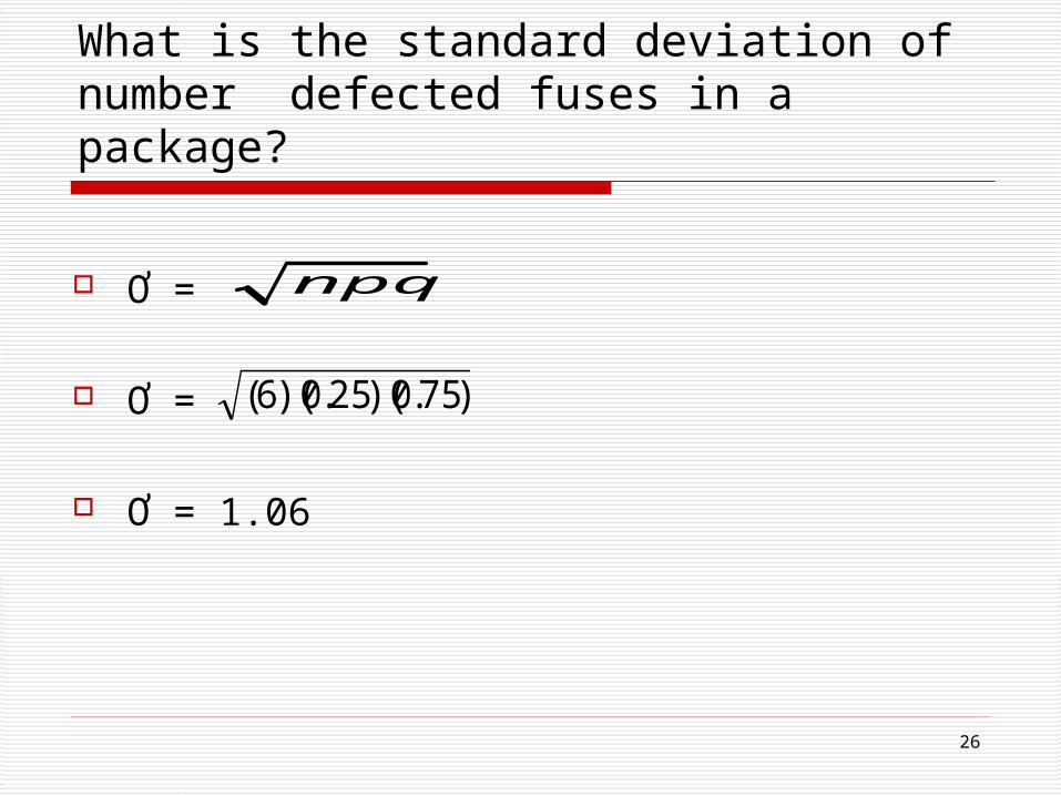
What is the standard deviation of number defected fuses in a package?

Ơ =

Ơ =

Ơ = 1.06

npq

)75.0)(25.0)(6(

27

What if we want to know the probability of obtaining 2 or more defected fuses? Cumulative Probability

p (x≥2) = p(2) + p(3) + p (4) + p(5) + p (6) p (x≥2) = 0.29663 + 0.13184+ 0.03296+ 0.00439+

0.00024 =0.46606

What if we want to know p (x≤2) ? p (x≤2) = p(0) + p(1) + p (2) p (x≤2) = 0.17798 + 0.35596 + 0.29663= 0.83057

28

Excel can generate binomial probability distribution

Page 660 of Stat Let’s do the same problem together Open excel Enter x into cell A1 Enter 0 and 1 into A2 and A3 Highlight A2 and A3 With left mouse grab the right hand corner

and drag until you see 6. Release the mouse

29

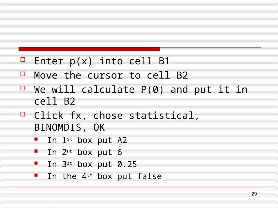
Enter p(x) into cell B1 Move the cursor to cell B2 We will calculate P(0) and put it in cell B2 Click fx, chose statistical, BINOMDIS, OK

In 1st box put A2 In 2nd box put 6 In 3rd box put 0.25 In the 4th box put false

30

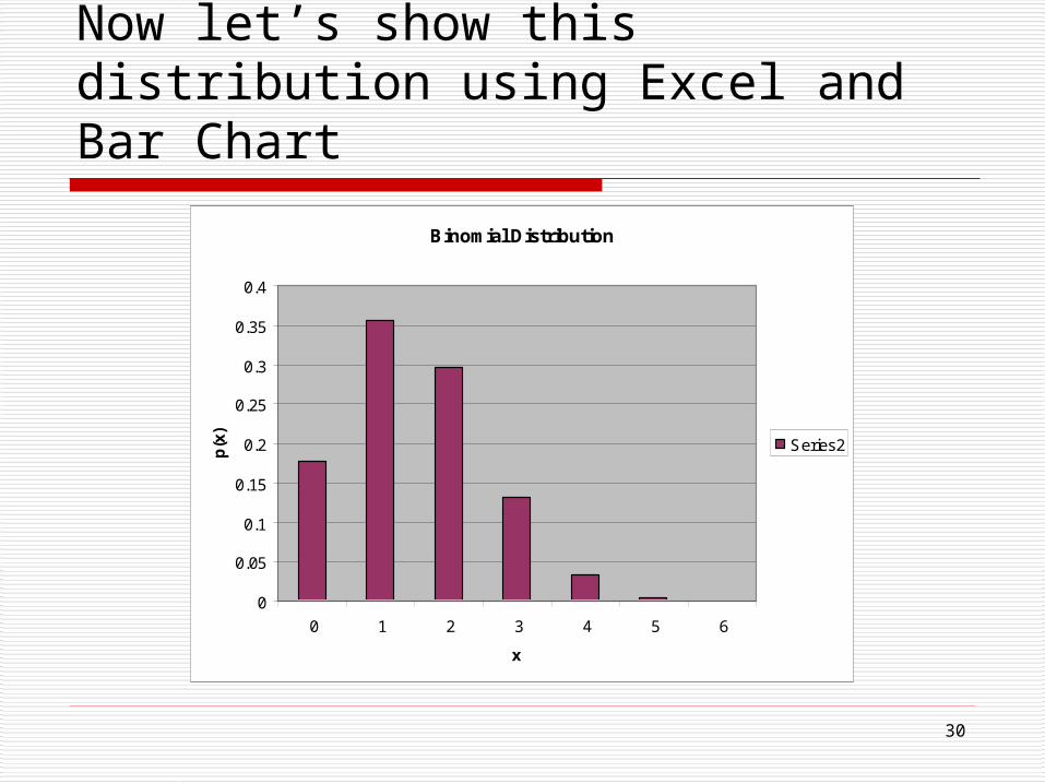
Now let’s show this distribution using Excel and Bar Chart

Binomial Distribution

0

0.05

0.1

0.15

0.2

0.25

0.3

0.35

0.4

0 1 2 3 4 5 6

x

p(x

)

Series2

31

Excel will also calculate cumulative p (x≤ …)

All you need to do is put “True” in the 4th box

32

Binomial probability table

Pages 602-608 Gives you cumulative probabilities for

less than or equal to Let’s try to use it for our problem

They don’t have p = 0.25 Take the average of 0.30 and 0.20

33

Chapter 6 of Econ

Reasons for covering this chapter Minimum wage Gas prices Taxes/subsidies

34

Price Ceiling

Government makes it illegal for anybody to charge higher than this price.

This is done to protect the consumers It is set below market equilibrium

price

35

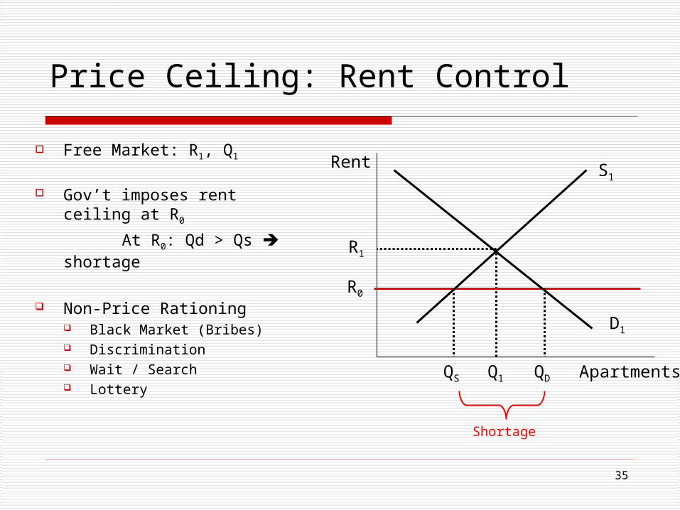
Price Ceiling: Rent Control

Free Market: R1, Q1

Gov’t imposes rent ceiling at R0

At R0: Qd > Qs shortage

Non-Price Rationing Black Market (Bribes) Discrimination Wait / Search Lottery Apartments

Rent

D1

S1

R1

Q1

R0

QS QD

Shortage

36

More on price ceiling

1. What happens if it is set above equilibrium?

It is not binding

2. What if over time demand becomes more elastic?

3. What if demand increases?4. What if supply increases?

37

Price Floor

Government makes it illegal for anybody to charge a price lower than this price.

This is done to protect the producers It is set above market equilibrium

price

38

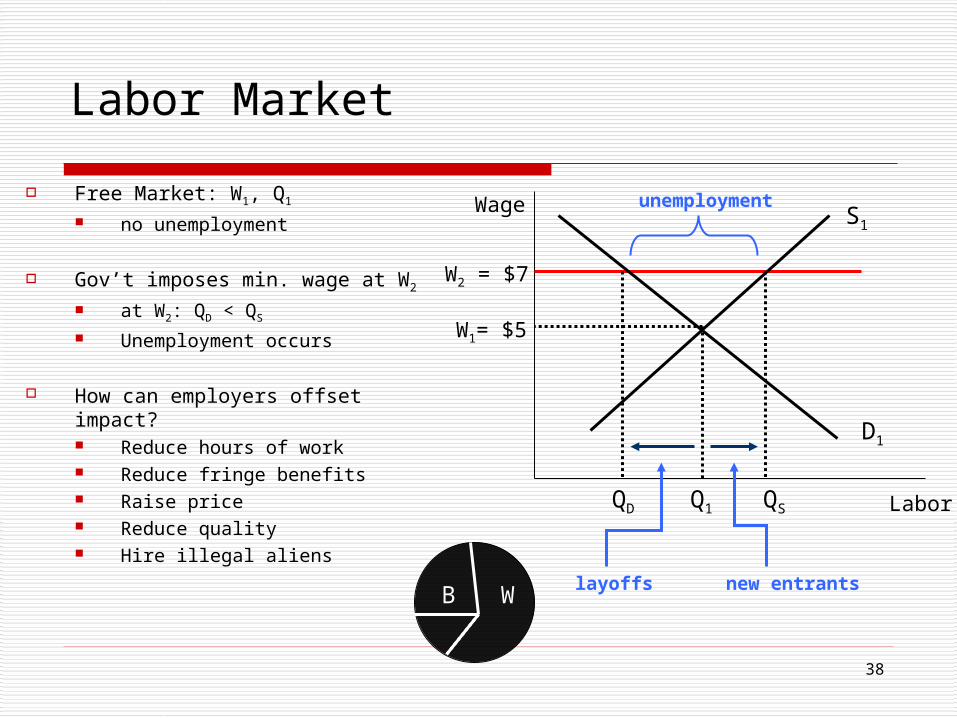
Labor Market

Free Market: W1, Q1

no unemployment

Gov’t imposes min. wage at W2

at W2: QD < QS

Unemployment occurs

How can employers offset impact? Reduce hours of work Reduce fringe benefits Raise price Reduce quality Hire illegal aliens

Labor

Wage

D1

S1

Q1

W2 = $7

unemployment

new entrantslayoffs

W1= $5

QD QS

WB

39

More on Price Floor

1. What happens if it is set below equilibrium?

It is not binding

2. What if over time demand becomes more elastic?

3. What if demand increases?4. What if supply increases?

40

The Minimum Wage, 1950-2006

0

1

2

3

4

5

6

7

8

9

1950 1955 1960 1965 1970 1975 1980 1985 1990 1995 2000 2005

Dol

lars

per

hou

r

minimum wage in current dollars

minimum wage in 2006 dollars

41

Minimum Wage Relative to the Average Private Nonsupervisory Wage

1950-2005

0%

10%

20%

30%

40%

50%

60%

1950 1955 1960 1965 1970 1975 1980 1985 1990 1995 2000 2005

42

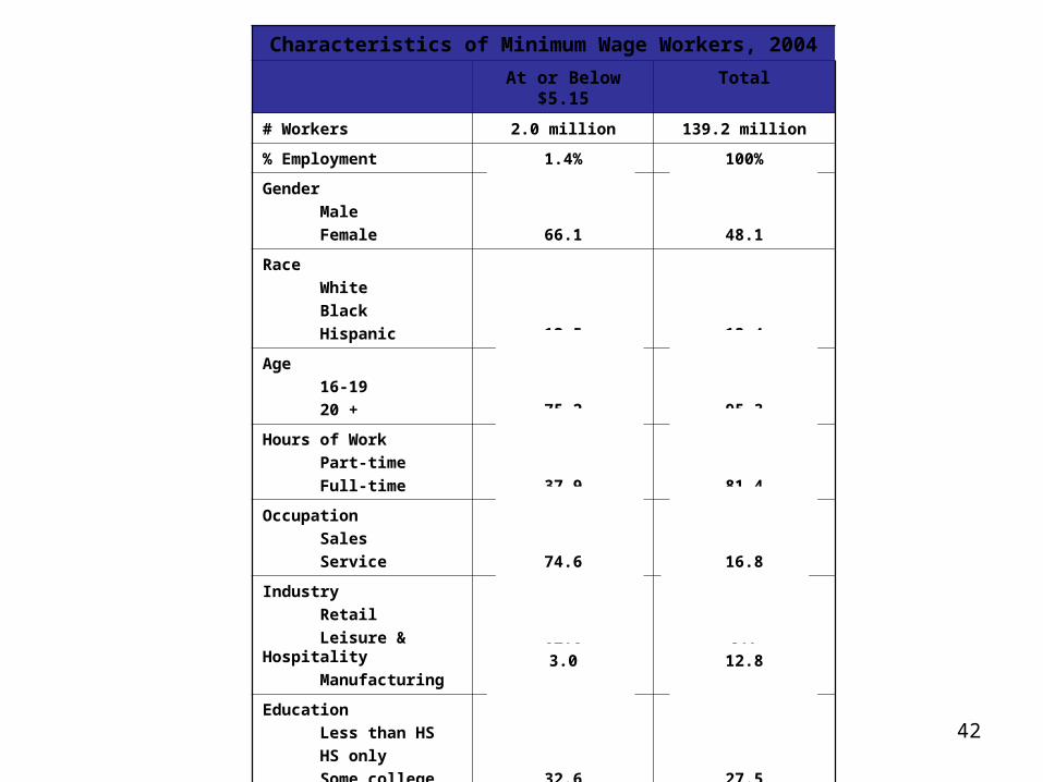
Characteristics of Minimum Wage Workers, 2004

At or Below $5.15 Total

# Workers 2.0 million 139.2 million

% Employment 1.4% 100%

Gender

Male

Female

33.9

66.1

51.9

48.1

Race

White

Black

Hispanic

83.9

11.3

12.5

69.6

11.1

13.4

Age

16-19

20 +

24.8

75.2

4.7

95.3

Hours of Work

Part-time

Full-time

61.9

37.9

18.6

81.4

Occupation

Sales

Service

12.6

74.6

10.9

16.8

Industry

Retail

Leisure & Hospitality

Manufacturing

8.2

62.0

3.0

11.9

8.7

12.8

Education

Less than HS

HS only

Some college

BA +

28.9

31.6

32.6

6.9

9.9

30.2

27.5

32.3