1

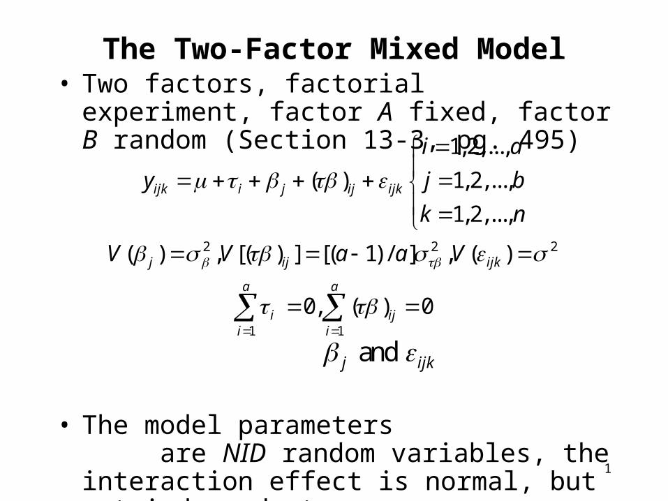
The Two-Factor Mixed Model• Two factors, factorial experiment, factor A fixed,

factor B random (Section 13-3, pg. 495)

• The model parameters are NID random variables, the interaction effect is normal, but not independent

• This is called the restricted model

2 2 2

1 1

1,2,...,

( ) 1, 2,...,

1, 2,...,

( ) , [( ) ] [( 1) / ] , ( )

0, ( ) 0

ijk i j ij ijk

j ij ijk

a a

i iji i

i a

y j b

k n

V V a a V

and j ijk

2

Testing Hypotheses - Mixed Model

• Once again, the standard ANOVA partition is appropriate

• Relevant hypotheses:

• Test statistics depend on the expected mean squares:

2 20 0 0

2 21 1 1

: 0 : 0 : 0

: 0 : 0 : 0

i

i

H H H

H H H

2

2 2 10

2 20

2 20

2

( ) 1

( )

( )

( )

a

ii A

AAB

BB

E

ABAB

E

E

bnMS

E MS n Fa MS

MSE MS an F

MS

MSE MS n F

MS

E MS

Ho is rejected if

Fo > F,a-1,(a-1)(b-1)

Fo > F,b-1,ab(n-1)

Fo > F,(a-1)(b-1), ab(n-1)

3

Estimating the Variance Components – Two Factor Mixed model

• Use the ANOVA method; equate expected mean squares to their observed values:

• Estimate the fixed effects (treatment means) as usual

2

2

2

ˆ

ˆ

ˆ

B E

AB E

E

MS MS

anMS MS

n

MS

.....

...ˆ

yy

y

ii

4

Example 13-3 (pg. 497) The Measurement Systems Capability

Study Revisited• Same experimental setting as in example 13-2• Parts are a random factor, but Operators are fixed• Assume the restricted form of the mixed model• Minitab can analyze the mixed model• The variance components can also be estimated as

99.0ˆ

14.02

99.071.0ˆ

23.10)2)(3(

99.039.62ˆ

2

2

2

E

EOperatorsPartsOperatorsParts

EPartsParts

MS

n

MSMS

an

MSMS

5

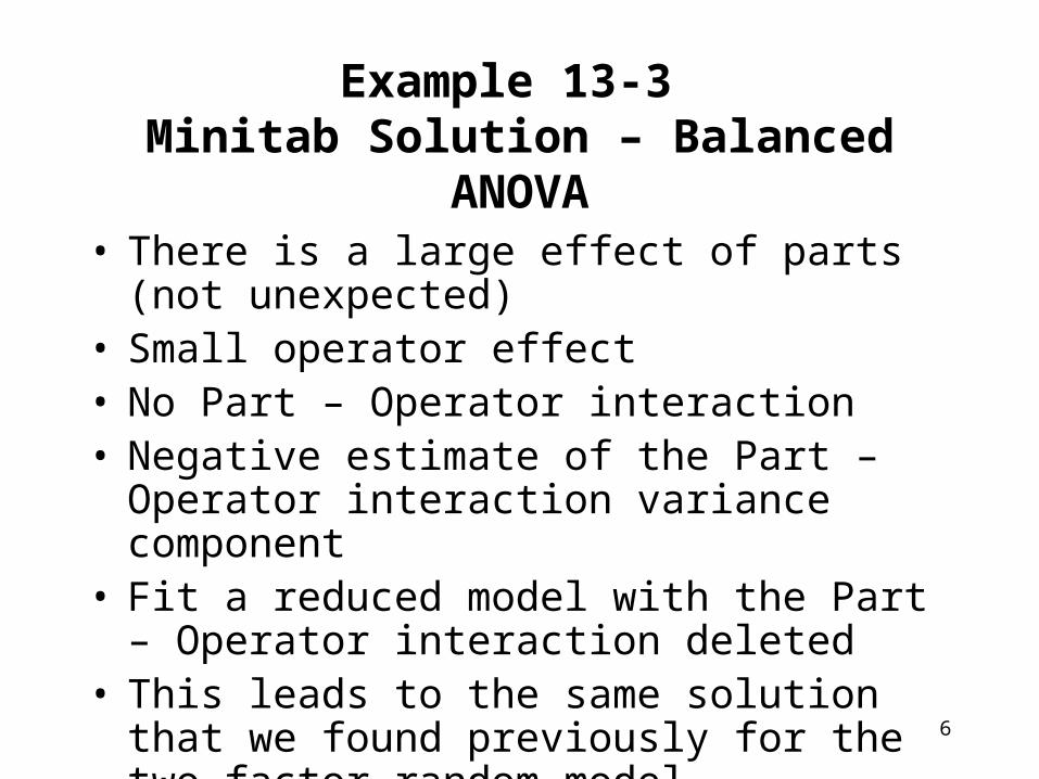
Example 13-3 (pg. 497) Minitab Solution – Balanced ANOVA

Source DF SS MS F P

Part 19 1185.425 62.391 62.92 0.000

Operator 2 2.617 1.308 1.84 0.173

Part*Operator 38 27.050 0.712 0.72 0.861

Error 60 59.500 0.992

Total 119 1274.592

Source Variance Error Expected Mean Square for Each Term

component term (using restricted model)

1 Part 10.2332 4 (4) + 6(1)

2 Operator 3 (4) + 2(3) + 40Q[2]

3 Part*Operator -0.1399 4 (4) + 2(3)

4 Error 0.9917 (4)

6

Example 13-3 Minitab Solution – Balanced ANOVA

• There is a large effect of parts (not unexpected)• Small operator effect• No Part – Operator interaction• Negative estimate of the Part – Operator

interaction variance component• Fit a reduced model with the Part – Operator

interaction deleted• This leads to the same solution that we found

previously for the two-factor random model

7

The Unrestricted Mixed Model• Two factors, factorial experiment, factor A fixed,

factor B random (pg. 498)

• The random model parameters are now all assumed to be NID . is no longer assumed – unrestricted model

0

)(,])[(,)(

,...,2,1

,...,2,1

,...,2,1

)(

1

222

a

ii

ijkijj

ijkijjiijk

VVV

nk

bj

ai

y

0)(1

a

i ij

8

Testing Hypotheses – Unrestricted Mixed Model

• The standard ANOVA partition is appropriate

• Relevant hypotheses:

• Expected mean squares determine the test statistics:

2 20 0 0

2 21 1 1

: 0 : 0 : 0

: 0 : 0 : 0

i

i

H H H

H H H

2

2 2 10

2 2 20

2 20

2

( ) 1

( )

( )

( )

a

ii A

AAB

BB

AB

ABAB

E

E

bnMS

E MS n Fa MS

MSE MS n an F

MS

MSE MS n F

MS

E MS

9

Estimating the Variance Components – Unrestricted Mixed Model

• Use the ANOVA method; equate expected mean squares to their observed values:

• The only change compared to the restricted mixed model is in the estimate of the random effect variance component

• Which model to use? o They are fairly close in many caseso The restricted model is slightly more generalo The restricted model is mostly preferred

2

2

2

ˆ

ˆ

ˆ

B AB

AB E

E

MS MS

anMS MS

n

MS

10

Example 13-4 (pg. 499) Minitab Solution – Unrestricted Model

Source DF SS MS F P

Part 19 1185.425 62.391 87.65 0.000

Operator 2 2.617 1.308 1.84 0.173

Part*Operator 38 27.050 0.712 0.72 0.861

Error 60 59.500 0.992

Total 119 1274.592

Source Variance Error Expected Mean Square for Each Term

component term (using unrestricted model)

1 Part 10.2798 3 (4) + 2(3) + 6(1)

2 Operator 3 (4) + 2(3) + Q[2]

3 Part*Operator -0.1399 4 (4) + 2(3)

4 Error 0.9917 (4)

11

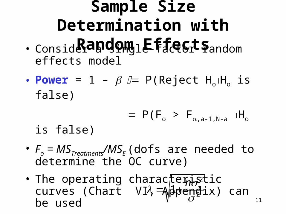
Sample Size Determination with Random Effects

• Consider a single-factor random effects model

• Power = 1 – P(Reject HoHo is false)

P(Fo > F,a-1,N-a Ho is false)

• Fo = MSTreatments/MSE (dofs are needed to determine the OC curve)

• The operating characteristic curves (Chart VI, Appendix) can be used

• The curves plot the probability of type II error against the parameter

2

2

1 n

12

Sample Size Determination with Random Effects – Example 13-5

• Five treatments randomly selected (a = 5)• Six observations per treatment (n = 6)• = 0.05, a – 1 = 4 (v1), N – a = 25 (v2)• Assume that • Then

0.20

646.2)1(61

22

13

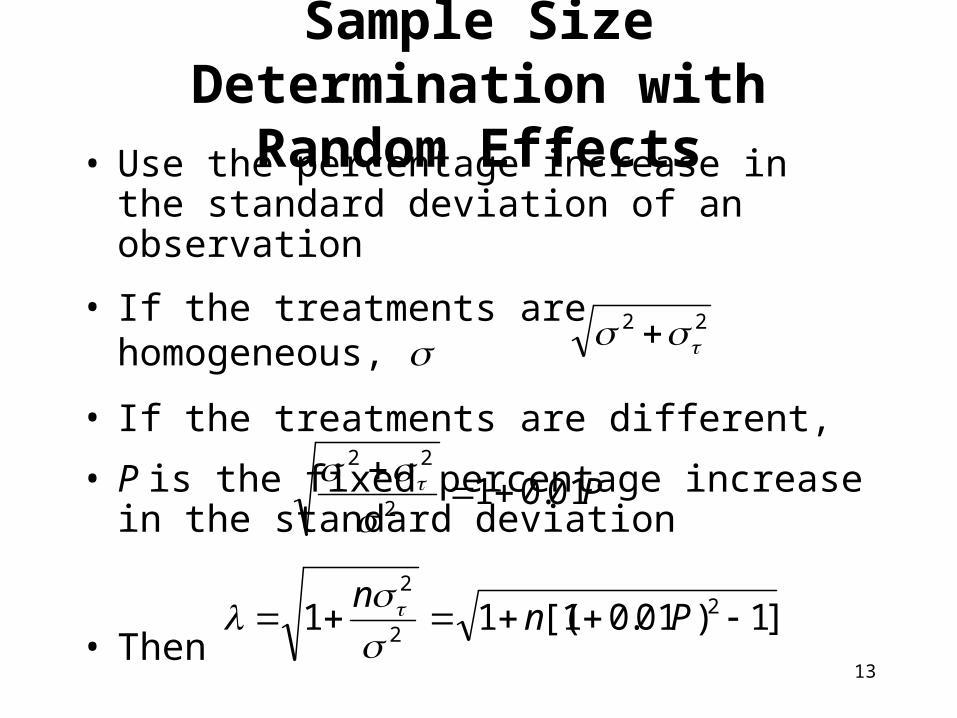
Sample Size Determination with Random Effects

• Use the percentage increase in the standard deviation of an observation

• If the treatments are homogeneous,

• If the treatments are different,

• P is the fixed percentage increase in the standard deviation

• Then

]1)01.01[(11 22

2

Pnn

22

P01.012

22

14

Sample Size Determination with Random Effects – Two Factors

Table 13-8

15

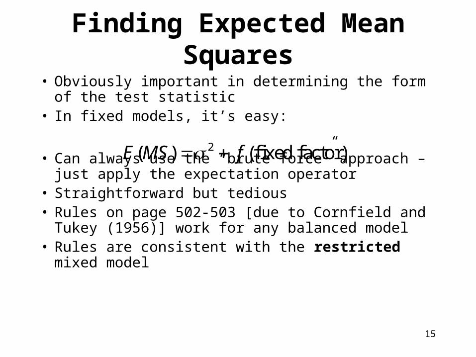
Finding Expected Mean Squares

• Obviously important in determining the form of the test statistic

• In fixed models, it’s easy:

• Can always use the “brute force” approach – just apply the expectation operator

• Straightforward but tedious• Rules on page 502-503 [due to Cornfield and Tukey

(1956)] work for any balanced model• Rules are consistent with the restricted mixed model

2( ) (fixed factor)E MS f

16

Approximate F Tests

• Sometimes we find that there are no exact tests for certain effects

17

Approximate F Tests• One possibility: assume that certain interactions are

negligible – needs conclusive evidence• If we cannot assume that certain interactions are

negligible, then use an approximate F test (“pseudo” F test)

• Test procedure is due to Satterthwaite (1946), and uses linear combinations of the original mean squares to form the F-ratio

• For example:

MS’ = MSr + …+ MSs

MS’’ = MSu + …+ MSv

• The mean squares are chosen so that E(MS’) – E(MS’’) is a multiple of the effect considered in the null hypothesis

• F is distributed approximately as Fp,q

SM

SMF

18

Approximate F Tests

• The linear combinations of the original mean squares are sometimes called “synthetic” mean squares

• Adjustments are required to the degrees of freedom

• Refer to Example 13-7, page 505• Minitab will analyze these experiments, although

their “synthetic” mean squares are not always the best choice