1 tensor voting: a perceptual organization approach to computer vision and machine learning...
Post on 20-Jan-2016
214 views
TRANSCRIPT
1
Tensor Voting: A Perceptual Organization
Approach to Computer Vision and Machine Learning
Philippos MordohaiUniversity of North Carolina, Chapel Hill
http://cs.unc.edu/~mordohai

2
Short Biography
• Ph.D. from University of Southern California with Gérard Medioni (2000-2005)– Perceptual organization– Binocular and multiple-view stereo– Feature inference from images– Figure completion– Manifold learning– Dimensionality estimation– Function approximation
• Postdoctoral researcher at University of North Carolina with Marc Pollefeys (2005-present)– Real-time video-based reconstruction of urban
environments– Multiple-view reconstruction– Temporally consistent video-based reconstruction
3
Audience
• Academia or industry?• Background:
– Perceptual organization– Image processing– Image segmentation– Human perception– 3-D computer vision– Machine learning
• Have you had exposure to tensor voting before?

4
Objectives
• Unified framework to address wide range of problems as perceptual organization
• Applications:– Computer vision problems– Instance-based learning
5
Overview
• Introduction• Tensor Voting• Stereo Reconstruction• Tensor Voting in N-D• Machine Learning• Boundary Inference • Figure Completion• More Tensor Voting Research• Conclusions
6
Motivation
• Computer vision problems are often inverse– Ill-posed– Computationally expensive– Severely corrupted by noise
• Many of them can be posed as perceptual grouping of primitives– Solutions form perceptually salient non-
accidental structures (e.g. surfaces in stereo)– Only input/output modules need to be adjusted
in most cases
7
Motivation
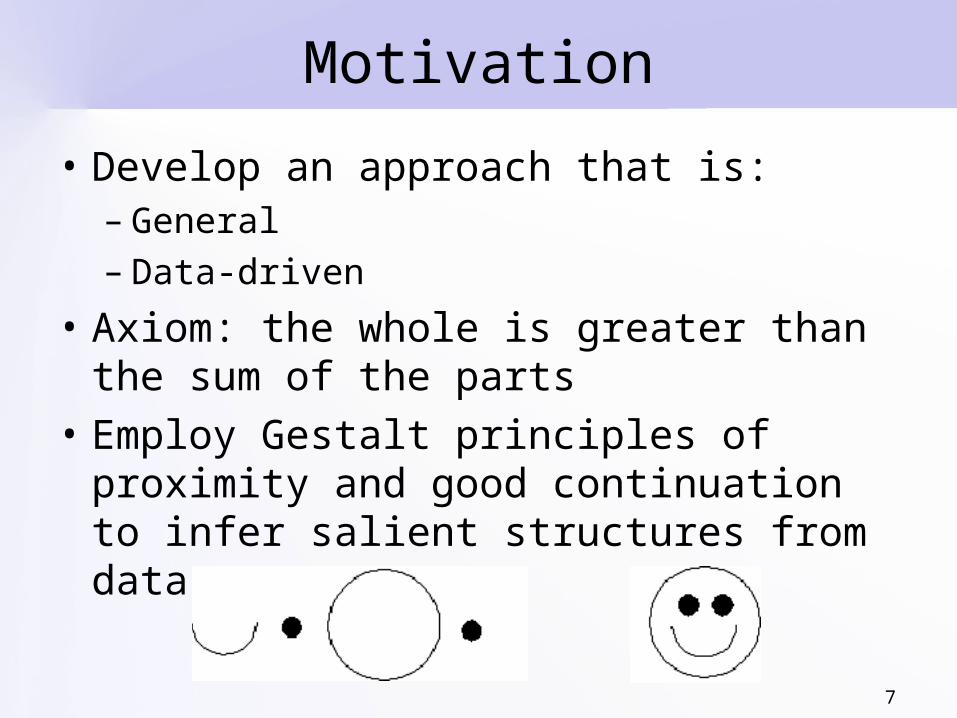
• Develop an approach that is:– General– Data-driven
• Axiom: the whole is greater than the sum of the parts
• Employ Gestalt principles of proximity and good continuation to infer salient structures from data
8
Gestalt Principles
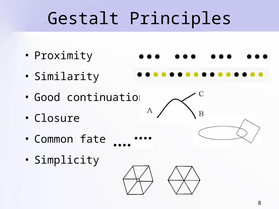
• Proximity
• Similarity
• Good continuation
• Closure
• Common fate
• Simplicity
9
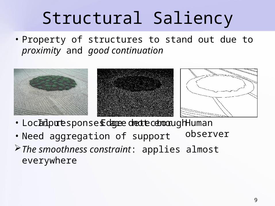
Structural Saliency• Property of structures to stand out due to
proximity and good continuation
• Local responses are not enough• Need aggregation of supportThe smoothness constraint: applies almost
everywhere
Input Human observerEdge detector
10
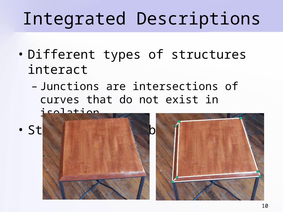
Integrated Descriptions
• Different types of structures interact – Junctions are intersections of curves that
do not exist in isolation
• Structures have boundaries

11
Desired Properties
• Local, data-driven descriptions– More general, model-free solutions– Local changes affect descriptions locally– Global optimization often requires simplifying
assumptions (NP-complete problems)
• Able to represent all structure types and their interactions
• Able to process large amounts of data
• Robust to noise
12
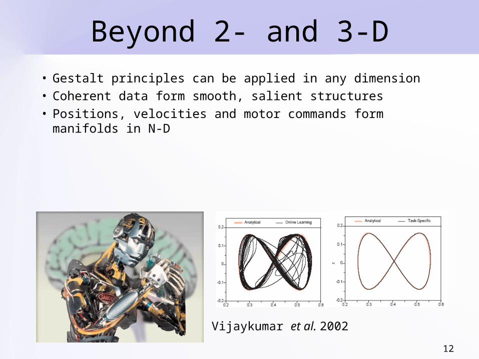
Beyond 2- and 3-D• Gestalt principles can be applied in any dimension• Coherent data form smooth, salient structures• Positions, velocities and motor commands form
manifolds in N-D
Vijaykumar et al. 2002
13
Perceptual Organization Approaches
• Symbolic methods
• Clustering
• Local interactions
• Inspired by human visual system
14
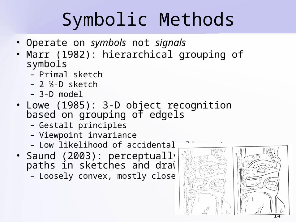
Symbolic Methods• Operate on symbols not signals• Marr (1982): hierarchical grouping of symbols
– Primal sketch– 2 ½-D sketch– 3-D model
• Lowe (1985): 3-D object recognition based on grouping of edgels– Gestalt principles– Viewpoint invariance– Low likelihood of accidental alignment
• Saund (2003): perceptually closed paths in sketches and drawings– Loosely convex, mostly closed

15
Symbolic Methods
• Mohan and Nevatia (1992): bottom-up hierarchical with increasing levels of abstraction– 3-D scene descriptions from collations of features
• Dolan and Riseman (1992): hierarchical curvilinear structure inference
• Jacobs (1996): salient convex groups as potential object outlines– Convexity, proximity,
contrast
16
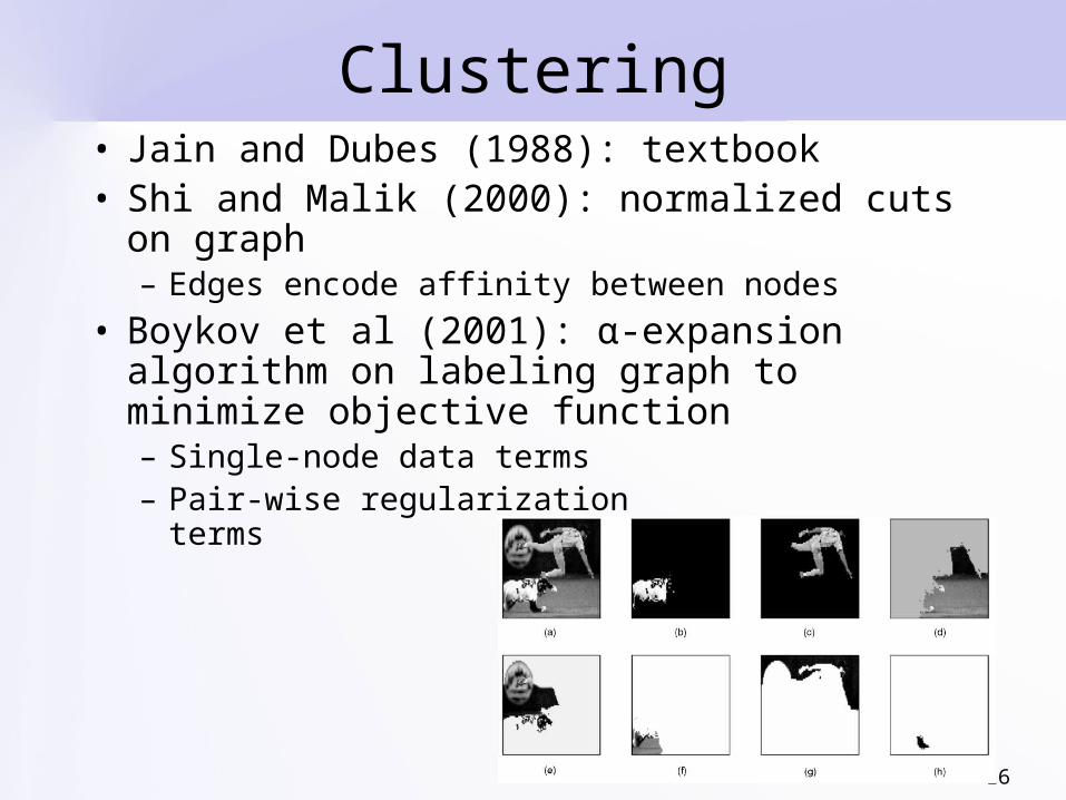
Clustering• Jain and Dubes (1988): textbook• Shi and Malik (2000): normalized cuts on
graph– Edges encode affinity between nodes
• Boykov et al (2001): α-expansion algorithm on labeling graph to minimize objective function– Single-node data terms– Pair-wise regularization
terms

17
Methods based on Local Interactions
• Shashua and Ullman (1988): structural saliency due to length and smoothness of curvature of curves going through each token
• Parent and Zucker (1989): trace points, tangents and curvature from noisy data
• Sander and Zucker (1990): 3-D extension• Guy and Medioni (1996, 1997):
predecessor of tensor voting– Voting fields– Tensor analysis for feature inference– Unified detection of surfaces,
curves and junctions
18
Inspired by Human Visual System
• Grossberg and Mingolla (1985), Grossberg and Todorovic (1988): Boundary Contour System and Feature Contour System– BCS: boundary detection, competition and cooperation,
includes cells that respond to “end-stopping”– FCS: surface diffusion mechanism limited by BCS
boundaries• Heitger and von der Heydt (1993): curvels
grouped into contours via convolution with orientation-selective kernels– Responses decay with distance, difference in
orientation– Detectors for endpoints, T-junctions and corners– Orthogonal and parallel grouping– Explain occlusion, illusory contours consistently with
perception
19
Inspired by Human Visual System
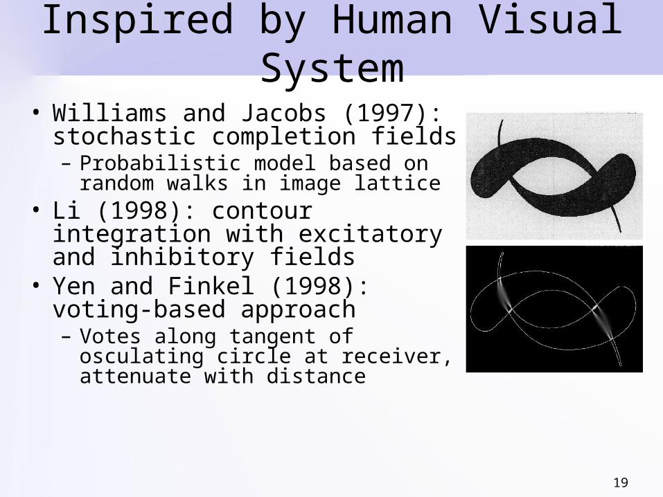
• Williams and Jacobs (1997): stochastic completion fields– Probabilistic model based on
random walks in image lattice• Li (1998): contour integration
with excitatory and inhibitory fields
• Yen and Finkel (1998): voting-based approach – Votes along tangent of osculating
circle at receiver, attenuate with distance
20
Differences with our Approach
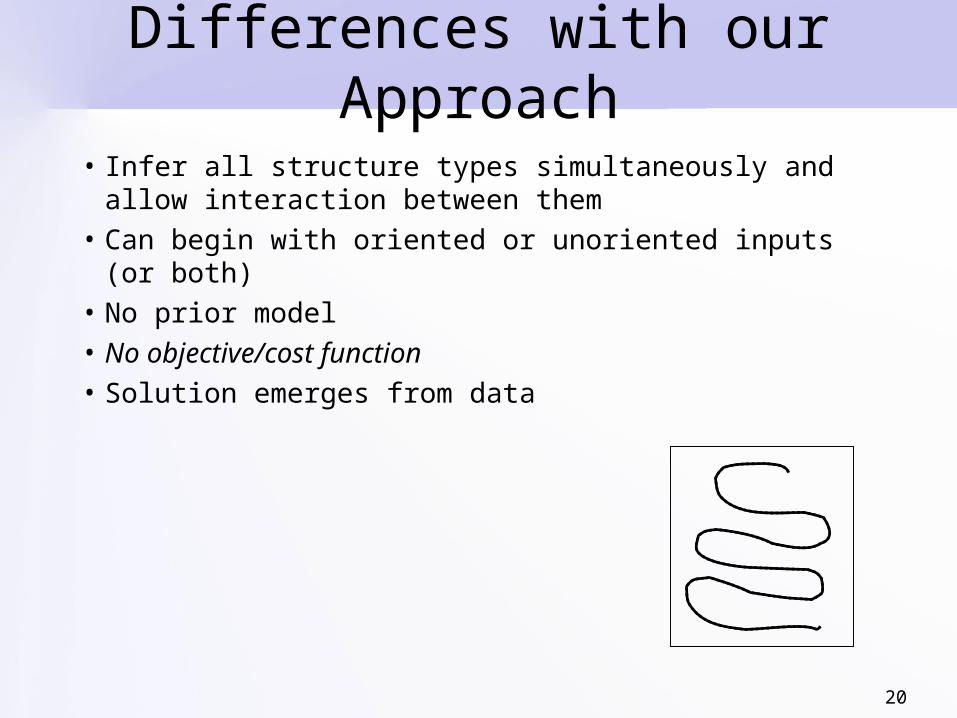
• Infer all structure types simultaneously and allow interaction between them
• Can begin with oriented or unoriented inputs (or both)
• No prior model• No objective/cost function• Solution emerges from data
21
Overview
• Introduction• Tensor Voting• Stereo Reconstruction• Tensor Voting in N-D• Machine Learning• Boundary Inference • Figure Completion• Conclusions
22
The Original Tensor Voting Framework
• Perceptual organization of generic tokens [Medioni, Lee, Tang 2000]
• Data representation: second order, symmetric, nonnegative definite tensors
• Information propagation: tensor voting• Infers saliency values and preferred
orientation for each type of structure
23
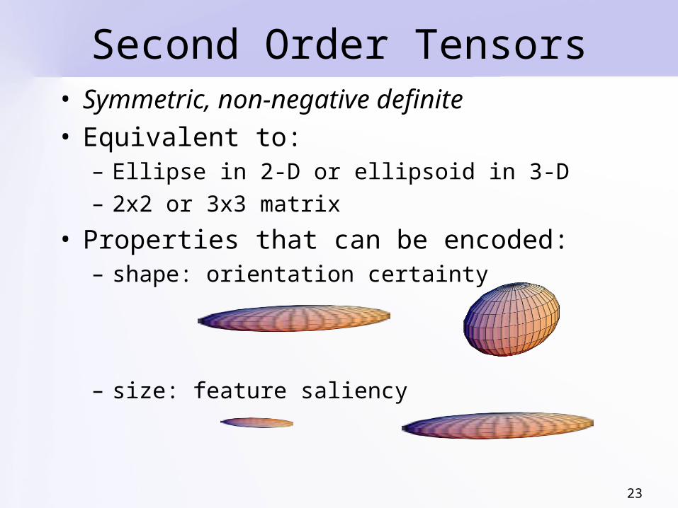
Second Order Tensors• Symmetric, non-negative definite• Equivalent to:
– Ellipse in 2-D or ellipsoid in 3-D– 2x2 or 3x3 matrix
• Properties that can be encoded:– shape: orientation certainty
– size: feature saliency

24
Second Order Tensors in 2-D
• 2×2 Matrix or Ellipse can be decomposed:– Stick component– Ball component
+=
00
02
22
22
22
222 b
aa
aa
aa
aba
)()( 221121121
222111
TTT
TT
eeeeee
eeeeT
25
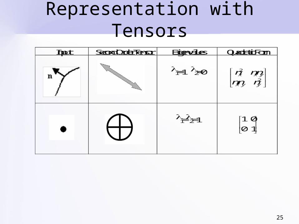
Representation with Tensors

26
Tensor Voting
?

27
Saliency Decay Function
• Votes attenuate with length of smooth path and curvature
• Stored in pre-computed voting fields
x
y
P
s
C
O
l
l
ls
sin2sin
28
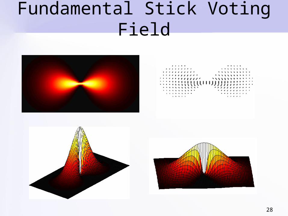
Fundamental Stick Voting Field
29
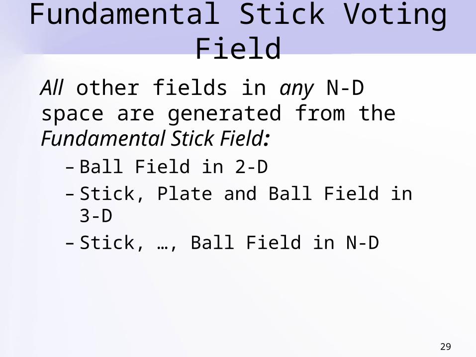
Fundamental Stick Voting Field
All other fields in any N-D space are generated from the Fundamental Stick Field:
– Ball Field in 2-D– Stick, Plate and Ball Field in 3-D– Stick, …, Ball Field in N-D
30
2-D Ball Field
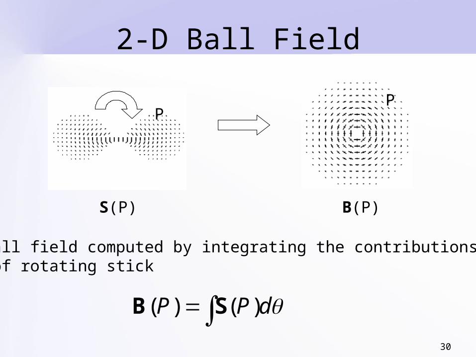
Ball field computed by integrating the contributions of rotating stick
dPP )()( SB
S(P) B(P)
PP
31
2-D Voting Fields
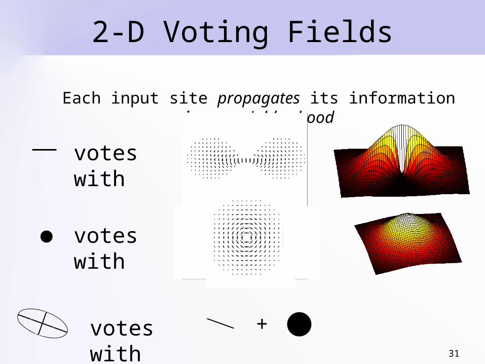
votes with
votes with
votes with +
Each input site propagates its information in a neighborhood

32
Voting
• Voting from a ball tensor is isotropic – Function of distance only
• The stick voting field is aligned with the orientation of the stick tensor
O
P

33
Scale of Voting
• The Scale of Voting is the single critical parameter in the framework
• Essentially defines size of voting neighborhood– Gaussian decay has infinite extend, but
it is cropped to where votes remain meaningful (e.g. 1% of voter saliency)
34
Scale of Voting
• The Scale is a measure of the degree of smoothness
• Smaller scales correspond to small voting neighborhoods, fewer votes– Preserve details– More susceptible to outlier corruption
• Larger scales correspond to large voting neighborhoods, more votes– Bridge gaps– Smooth perturbations– Robust to noise
35
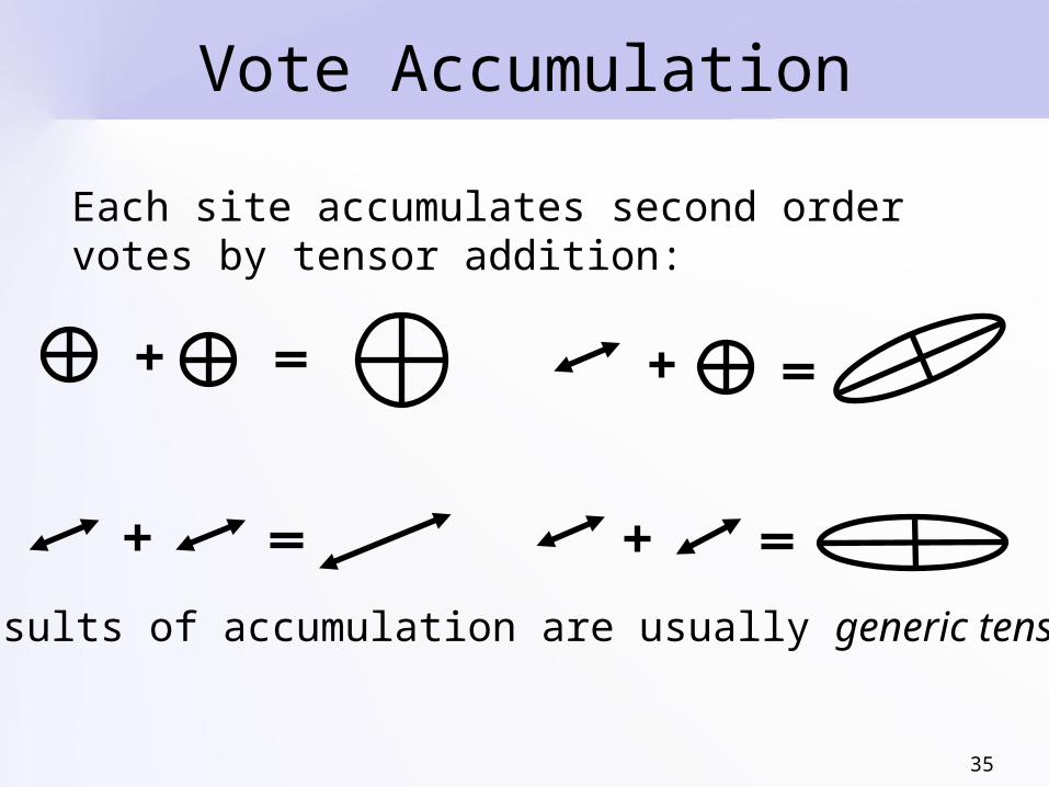
Vote Accumulation
Each site accumulates second order votes by tensor addition:
Results of accumulation are usually generic tensors
36
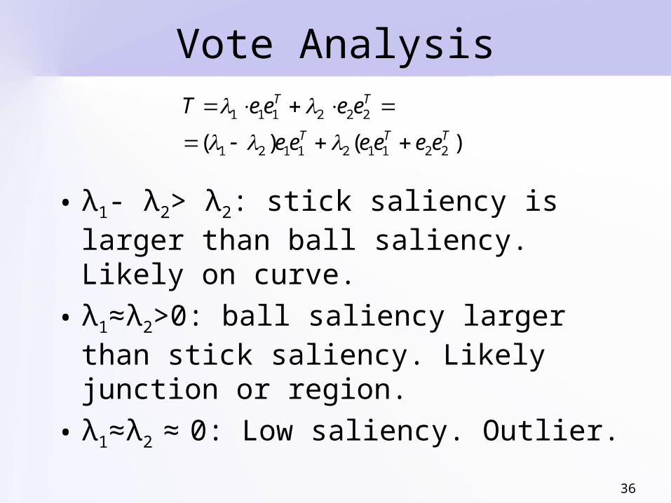
Vote Analysis
• λ1- λ2> λ2: stick saliency is larger than ball saliency. Likely on curve.
• λ1≈λ2>0: ball saliency larger than stick saliency. Likely junction or region.
• λ1≈λ2 ≈ 0: Low saliency. Outlier.
)()( 221121121
222111
TTT
TT
eeeeee
eeeeT
37
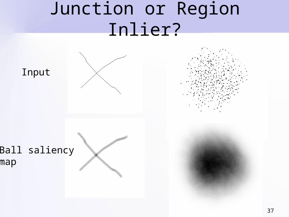
Junction or Region Inlier?
Input
Ball saliencymap
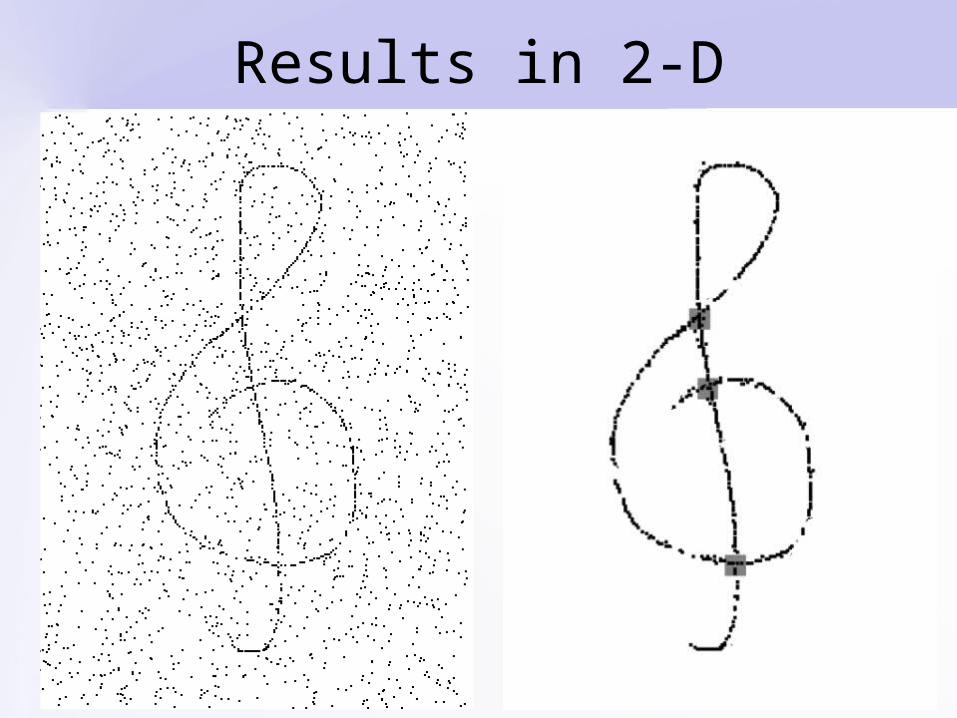
38
Results in 2-D
39
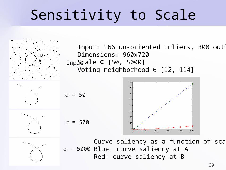
Sensitivity to Scale
AB
Input
= 50
= 500
= 5000Curve saliency as a function of scaleBlue: curve saliency at ARed: curve saliency at B
Input: 166 un-oriented inliers, 300 outliersDimensions: 960x720Scale ∈ [50, 5000] Voting neighborhood ∈ [12, 114]

40
Sensitivity to Scale
Circle with radius 100 (unoriented tokens)
As more information is accumulated, the tokens better approximate the circle
41
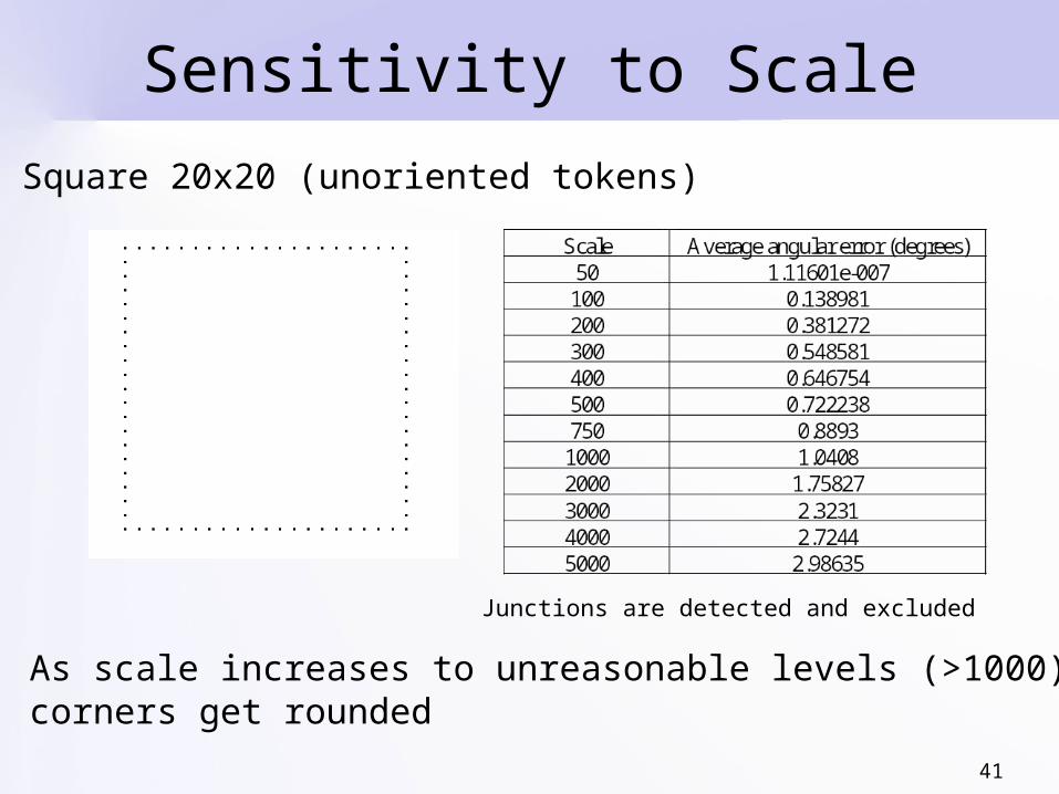
Sensitivity to Scale
Square 20x20 (unoriented tokens)
As scale increases to unreasonable levels (>1000)corners get rounded
Junctions are detected and excluded
42
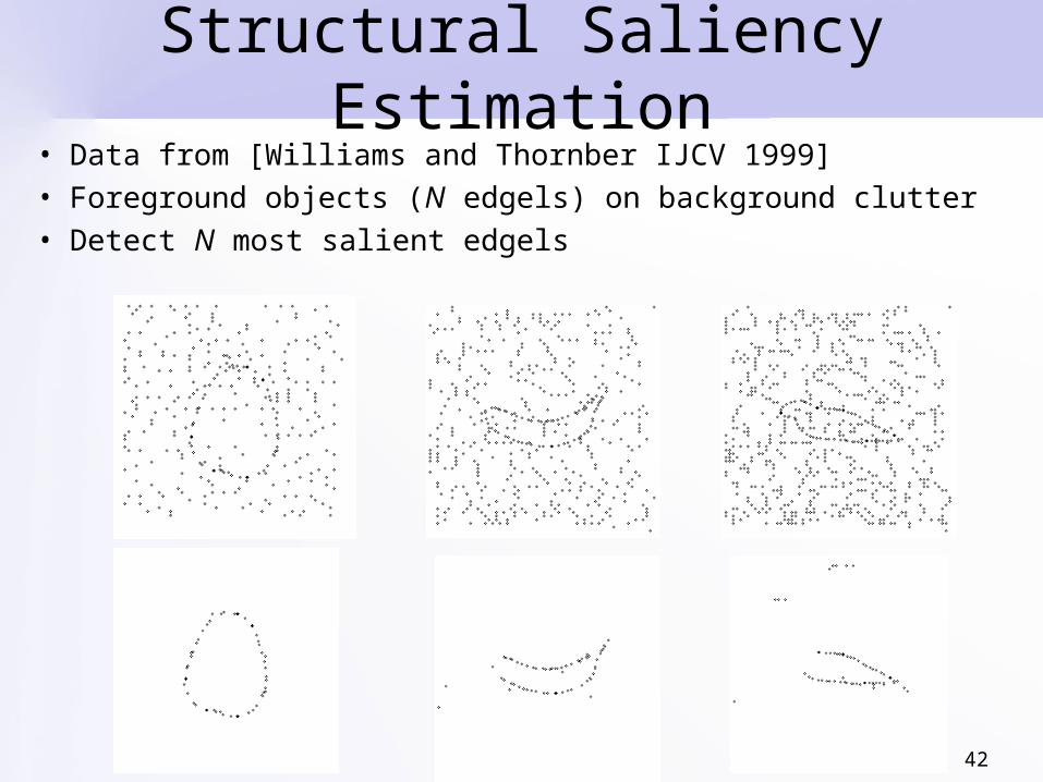
Structural Saliency Estimation• Data from [Williams and Thornber IJCV 1999]• Foreground objects (N edgels) on background clutter• Detect N most salient edgels

43
Structural Saliency Estimation
• SNR: ratio of foreground edgels to background edgels
• FPR: false positive rate for foreground detection
• Our results outperform all methods evaluated in [Williams and Thornber IJCV 1999]
SNR 25 20 15 10 5
FPR 10.0%
12.4%
18.4%
35.8%
64.3%

44
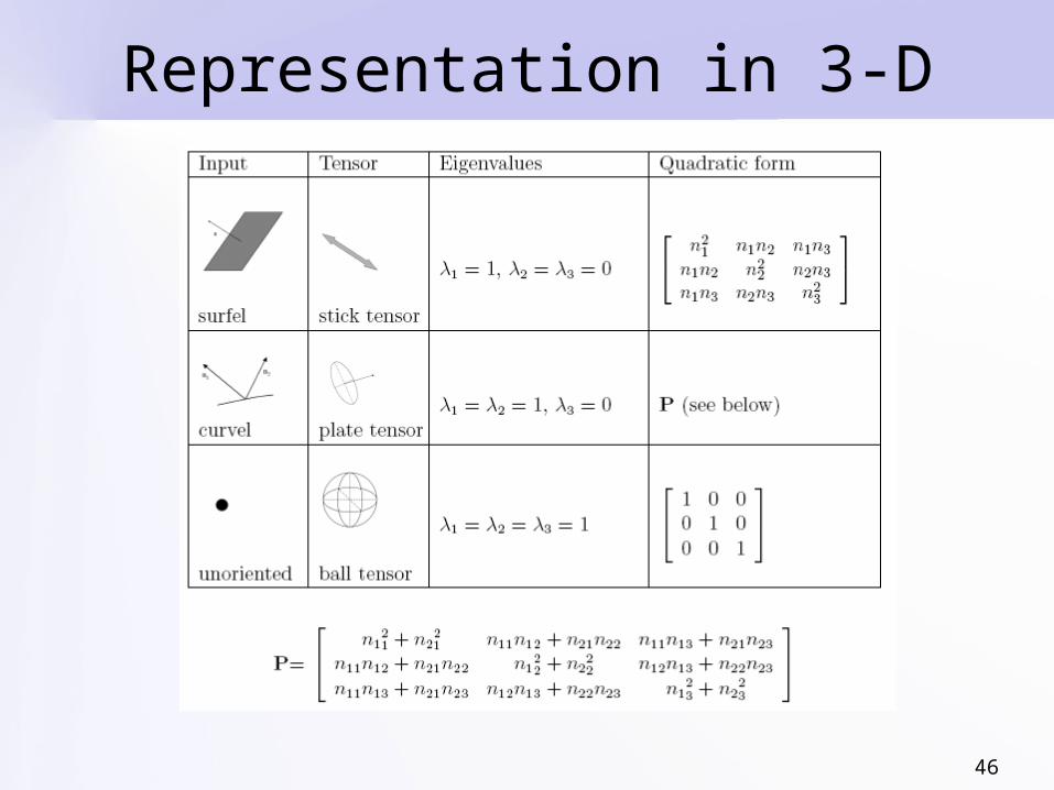
Structure Types in 3-D
The input may consist of
point/junction curvel
surfel

45
3-D Second Order Tensors
• Encode normal orientation in tensor
• Surfel: 1 normal “stick” tensor
• Curvel: 2 normals “plate” tensor
• Point/junction: 3 normals “ball” tensor
46
Representation in 3-D

47
3-D Tensor Analysis
• Surface saliency: λ1- λ2 normal: e1
• Curve saliency: λ2- λ3 normals: e1 and e2
• Junction saliency: λ3
)())(()( 33221132211321121
333222111
TTTTTT
TTT
eeeeeeeeeeee
eeeeee
T
48
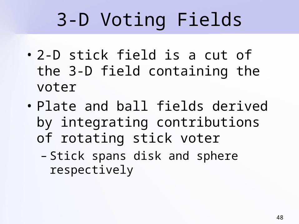
3-D Voting Fields
• 2-D stick field is a cut of the 3-D field containing the voter
• Plate and ball fields derived by integrating contributions of rotating stick voter– Stick spans disk and sphere
respectively
49
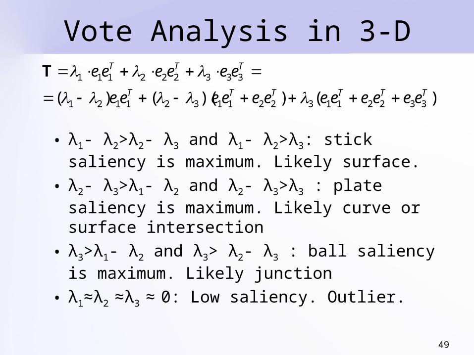
Vote Analysis in 3-D
• λ1- λ2>λ2- λ3 and λ1- λ2>λ3: stick saliency is maximum. Likely surface.
• λ2- λ3>λ1- λ2 and λ2- λ3>λ3 : plate saliency is maximum. Likely curve or surface intersection
• λ3>λ1- λ2 and λ3> λ2- λ3 : ball saliency is maximum. Likely junction
• λ1≈λ2 ≈λ3 ≈ 0: Low saliency. Outlier.
)())(()( 33221132211321121
333222111
TTTTTT
TTT
eeeeeeeeeeee
eeeeee
T
50
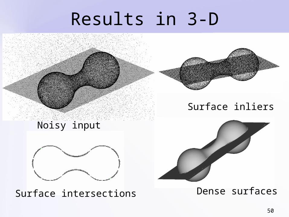
Results in 3-D
Noisy input
Surface intersections Dense surfaces
Surface inliers

51
Overview
• Introduction• Tensor Voting• Stereo Reconstruction• Tensor Voting in N-D• Machine Learning• Boundary Inference • Figure Completion• More Tensor Voting Research• Conclusions

52
Approach for Stereo
• Problem can be posed as perceptual organization in 3-D – Correct pixel matches should form
smooth, salient surfaces in 3-D– 3-D surfaces should dictate pixel
correspondences• Infer matches and surfaces by
tensor voting• Use monocular cues to
complement binocular matches [Mordohai and Medioni, ECCV 2004 and PAMI 2006]
53
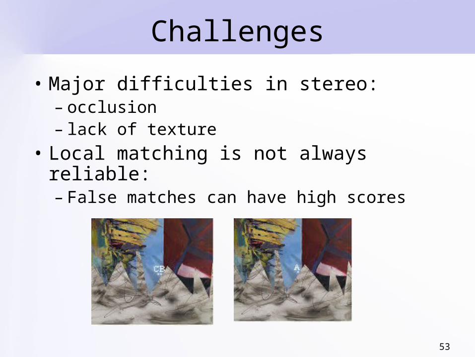
Challenges
• Major difficulties in stereo: – occlusion – lack of texture
• Local matching is not always reliable:– False matches can have high scores
54
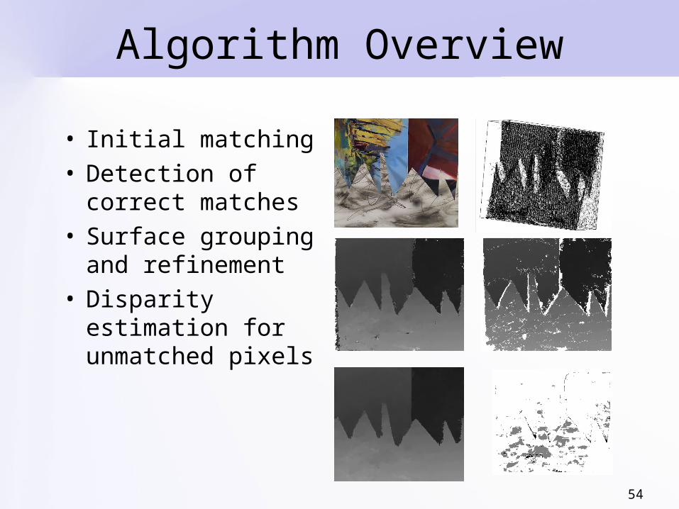
Algorithm Overview
• Initial matching• Detection of
correct matches • Surface grouping
and refinement• Disparity
estimation for unmatched pixels
55
Initial Matching
• Each matching technique has different strengths
• Use multiple techniques and both images as reference:– 5×5 normalized cross correlation (NCC)
window– 5×5 shiftable NCC window– 25×25 NCC window for pixels with very low
color variance– 7×7 symmetric interval matching window
with truncated cost function
Note: small windows produce random (not systematic) errors (reduced foreground fattening)
56
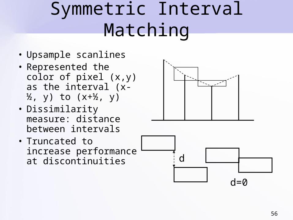
Symmetric Interval Matching
• Upsample scanlines• Represented the color
of pixel (x,y) as the interval (x-½, y) to (x+½, y)
• Dissimilarity measure: distance between intervals
• Truncated to increase performance at discontinuities
d
d=0

57
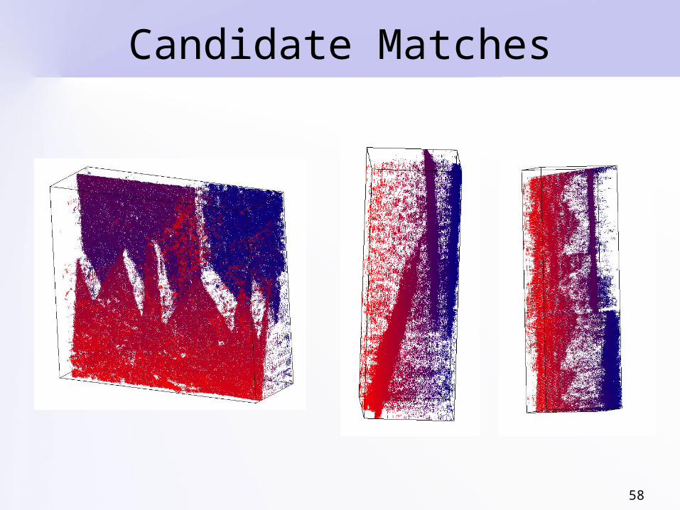
Candidate Matches
• Compute sub-pixel estimates (parabolic fit)
• Keep all good matches (peaks of NCC)• Drop scores
– Depend on texture properties– Hard to combine across methods
58
Candidate Matches
59
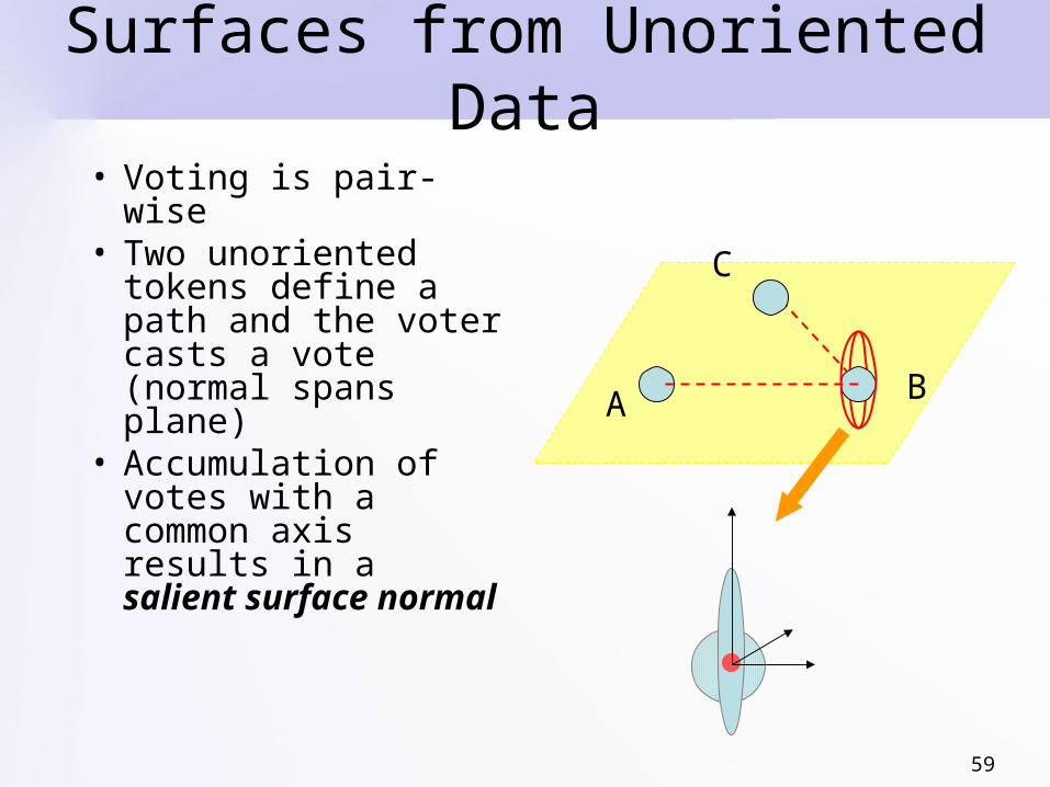
Surfaces from Unoriented Data
• Voting is pair-wise• Two unoriented
tokens define a path and the voter casts a vote (normal spans plane)
• Accumulation of votes with a common axis results in a salient surface normal
A
C
B
60
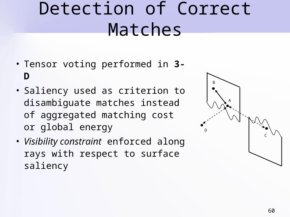
Detection of Correct Matches
• Tensor voting performed in 3-D
• Saliency used as criterion to disambiguate matches instead of aggregated matching cost or global energy
• Visibility constraint enforced along rays with respect to surface saliency
A
CD
B

61
Uniqueness vs. Visibility
• Uniqueness constraint: One-to-one pixel correspondence– Exact only for fronto-parallel surfaces
• Visibility constraint : M-to-N pixel correspondences– [Ogale and Aloimonos 2004][Sun et al.
2005]– One match per ray of each camera
62
Surface Grouping
• Image segmentation has been shown to help stereo – Not an easier problem
• Instead, group candidate matches in 3-D based on geometric properties– Pick most salient candidate matches as
seeds– Grow surfaces
• Represent surfaces as local collections of colors
63
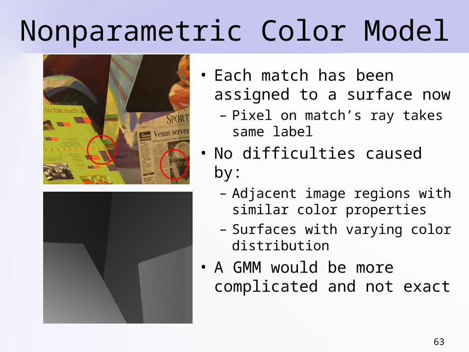
Nonparametric Color Model• Each match has been
assigned to a surface now– Pixel on match’s ray takes
same label
• No difficulties caused by:– Adjacent image regions with
similar color properties – Surfaces with varying color
distribution
• A GMM would be more complicated and not exact
64
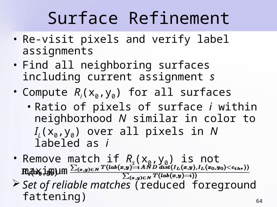
Surface Refinement• Re-visit pixels and verify label assignments• Find all neighboring surfaces including current
assignment s• Compute Ri(x0,y0) for all surfaces
• Ratio of pixels of surface i within neighborhood N similar in color to IL(x0,y0) over all pixels in N labeled as i
• Remove match if Rs(x0,y0) is not maximum Set of reliable matches (reduced foreground fattening)

65
Surface Refinement Results
144808 matches4278 errors
136894 matches1481 errors

66
Surface Refinement Results
84810 matches4502 errors
69666 matches928 errors
67
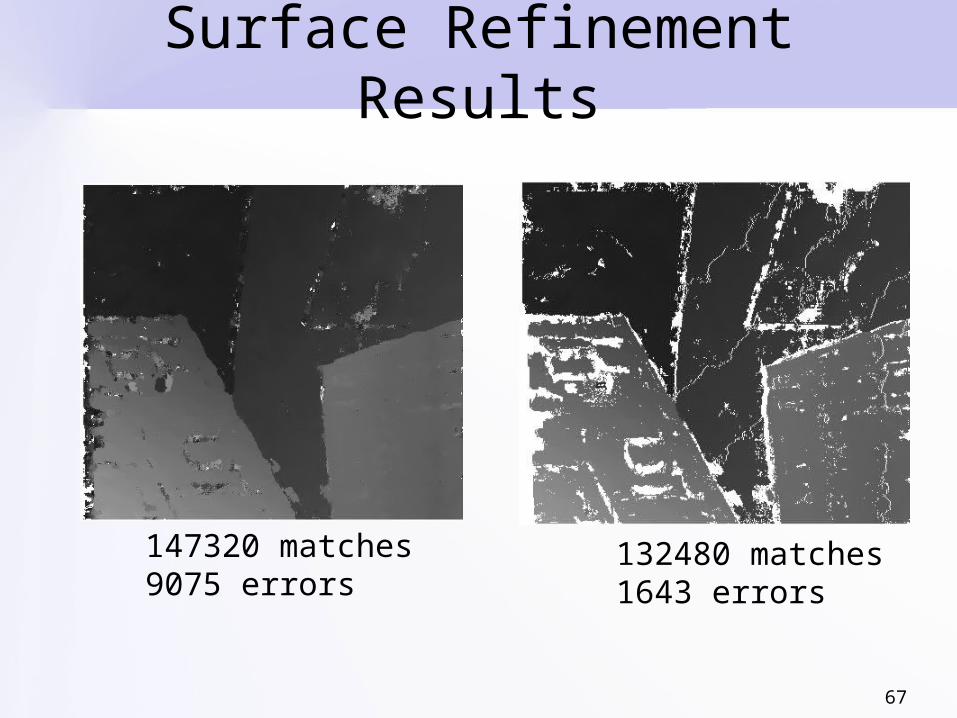
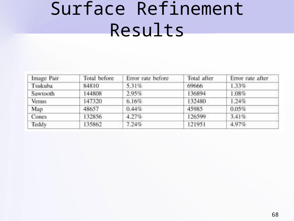
Surface Refinement Results
147320 matches9075 errors
132480 matches1643 errors
68
Surface Refinement Results

69
Disparity Hypotheses for Unmatched Pixels
• Check color consistency with nearby layers (on both images if not occluded)
• Generate hypotheses for membership in layers with similar color properties– Find disparity range from
neighbors (and extend)– Allow occluded hypotheses– Do not allow occlusion of
reliable matches
• Progressively increase color similarity tolerance and scale
70
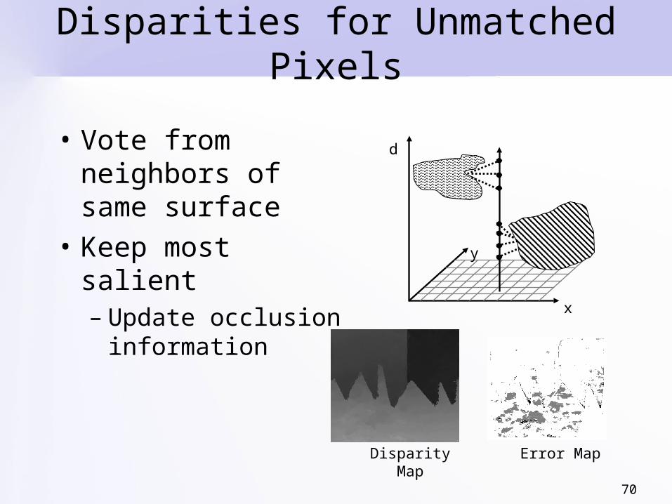
Disparities for Unmatched Pixels
• Vote from neighbors of same surface
• Keep most salient– Update occlusion
information
d
x
y
Disparity Map Error Map
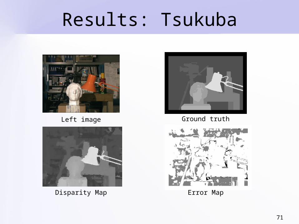
71
Results: Tsukuba
Left image Ground truth
Error MapDisparity Map

72
Results: Venus
Left image Ground truth
Error MapDisparity Map
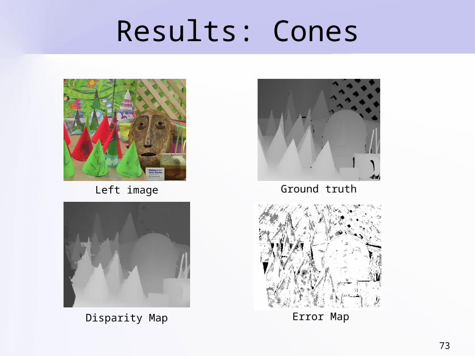
73
Results: Cones
Left image Ground truth
Error MapDisparity Map
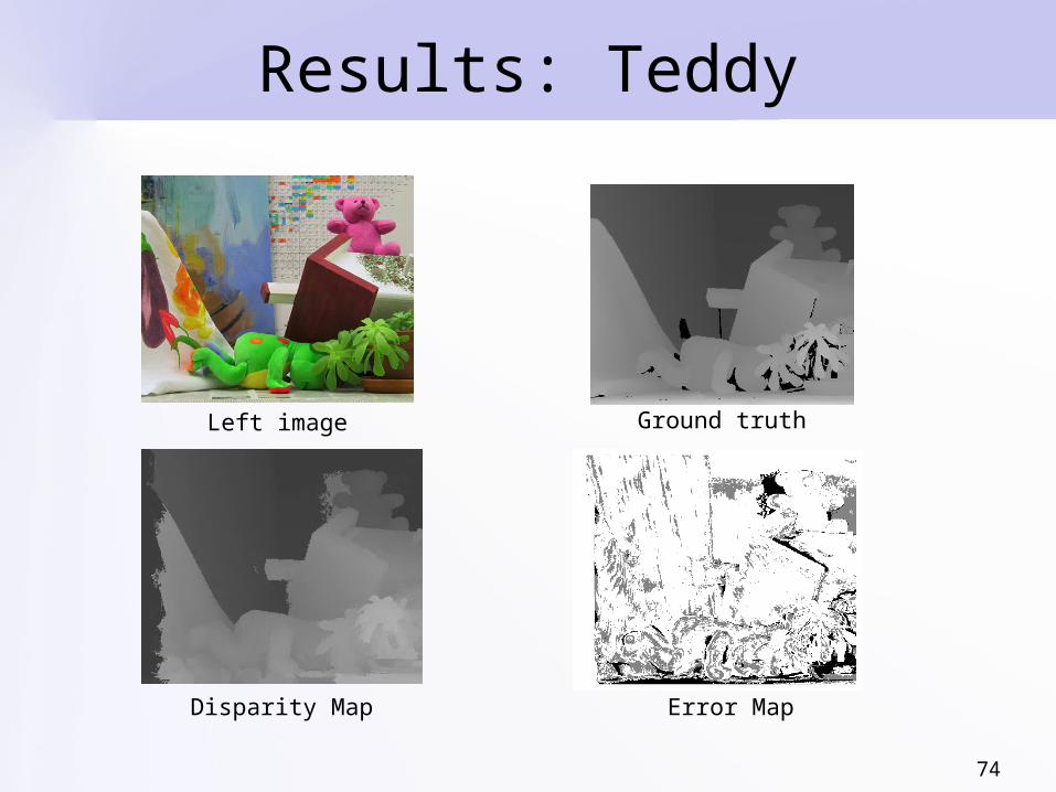
74
Results: Teddy
Left image Ground truth
Error MapDisparity Map
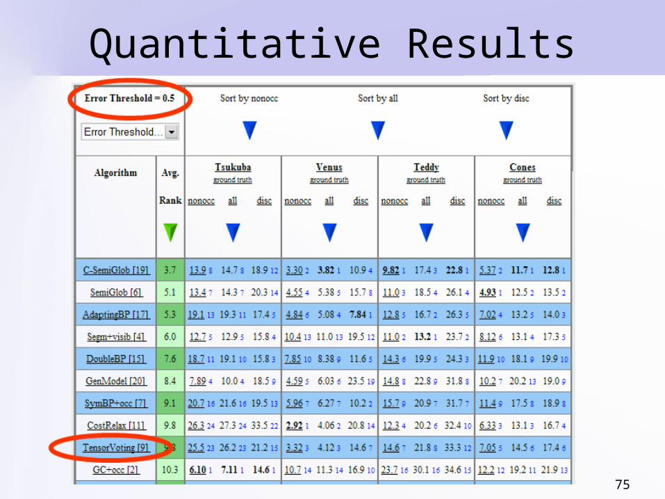
75
Quantitative Results

76
Aerial Images
77
Summary of Approach to Stereo
• Binocular and monocular cues are combined• Novel initial matching framework• No image segmentation • Occluding surfaces do not over-extend
because of color consistency requirement• Textureless surfaces are inferred based on
surface smoothness– When initial matching fails
78
Multiple-View Stereo
• Approach to dense multiple-view stereo– Multiple views: more than two– Dense: attempt to reconstruct all pixels
• Process all data simultaneously– Do not rely on binocular results– Only binocular step: detection of potential pixel
correspondences
• Correct matches form coherent salient surfaces– Infer them by Tensor Voting
[Mordohai and Medioni, 3DPVT 2004]

79
Desired Properties
• General camera placement – As long as camera pairs are close enough for
automatic pixel matching• No privileged images• Features required to appear in no more
than two images• Reconstruct background
– Do not discard• Simultaneous processing
– Do not merge binocular results

80
Input Images
Captured at the CMU dome for the Virtualized Reality project

81
Limitations of Binocular Processing
Errors due to:– Occlusion– Lack of texture
Matching candidates in disparity space Disparity map after binocular processing
82
Limitations of Binocular Processing
When matching from many image pairs, candidates are combined:
– Lessens effects of depth discontinuities• Occluded surfaces are revealed
– Salient surfaces are reinforced by correct matches from multiple pairs• Noise is not
83
Candidate Matches
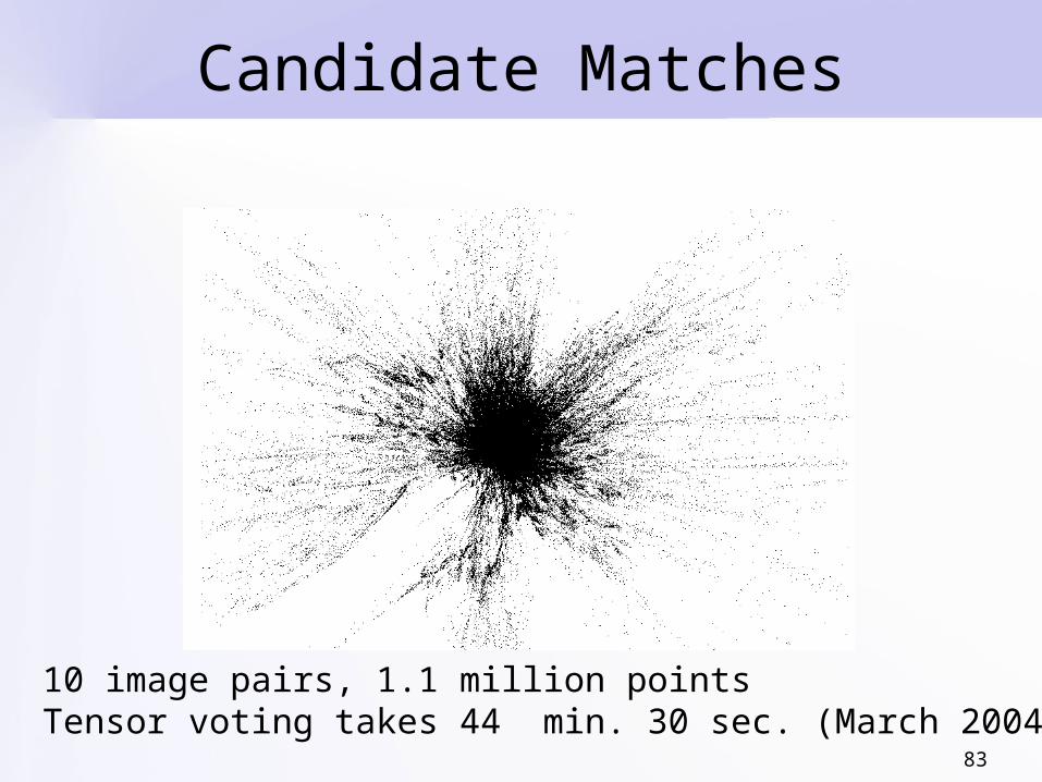
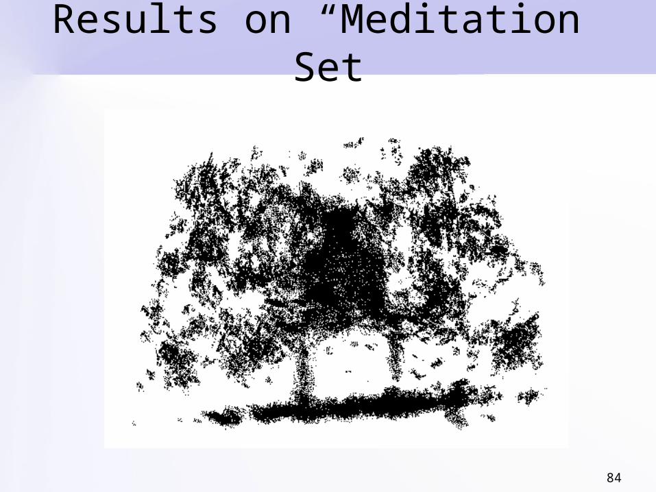
10 image pairs, 1.1 million pointsTensor voting takes 44 min. 30 sec. (March 2004)
84
Results on “Meditation” Set

85
Results on “Meditation” Set

86
Results on “Baseball” Dataset

87
Overview
• Introduction• Tensor Voting• Stereo Reconstruction• Tensor Voting in N-D• Machine Learning• Boundary Inference • Figure Completion• More Tensor Voting Research• Conclusions
88
Tensor Representation in N-D• Non-accidental alignment, proximity, good
continuation apply in N-D– Robot arm moving from point to point forms 1-D
trajectory (manifold) in N-D space• Noise robustness and ability to represent all
structure types also desirable
• Tensor construction: – eigenvectors of normal space associated with
non-zero eigenvalues– eigenvectors of tangent space associated with
non-zero eigenvalues
[Mordohai, PhD Thesis 2005]
89
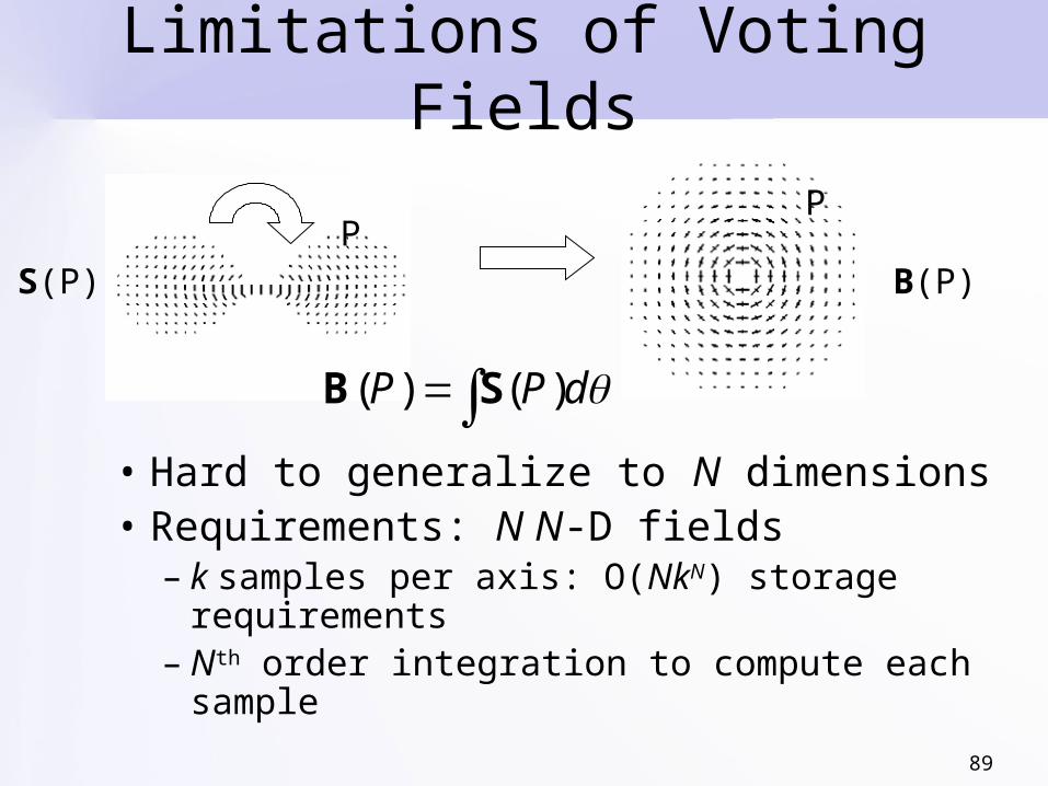
Limitations of Voting Fields
• Hard to generalize to N dimensions• Requirements: N N-D fields
– k samples per axis: O(NkN) storage requirements
– Nth order integration to compute each sample
S(P) B(P)P
P
dPP )()( SB
90
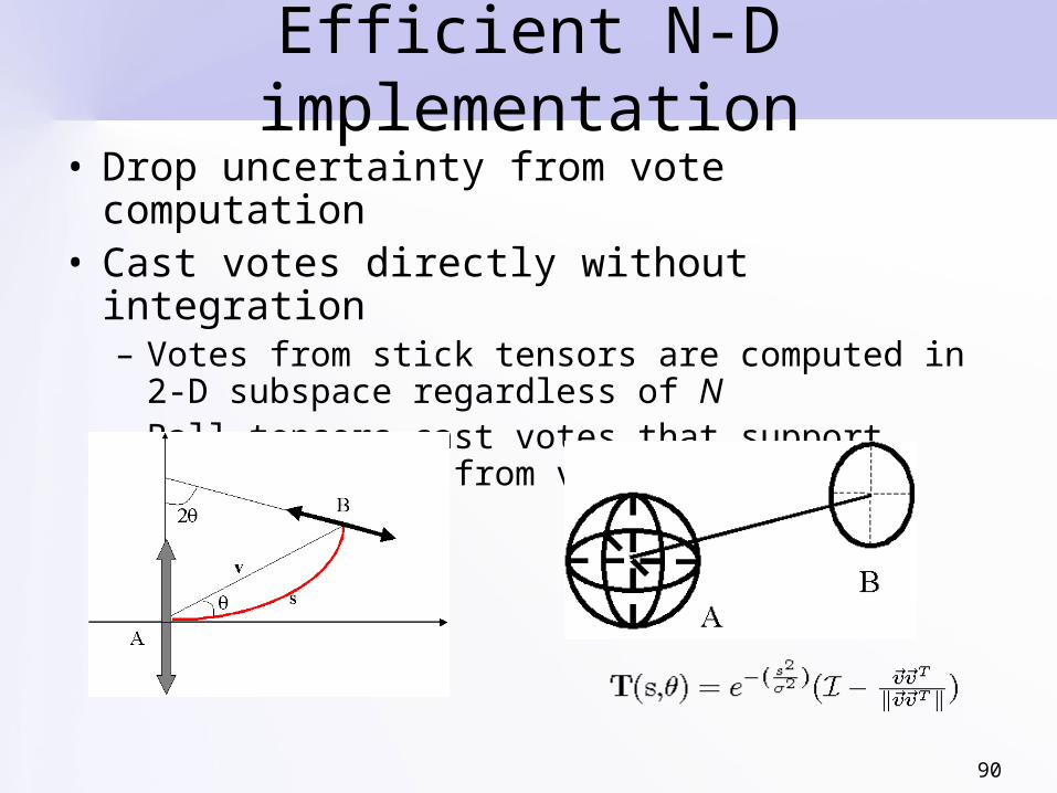
Efficient N-D implementation• Drop uncertainty from vote computation• Cast votes directly without integration
– Votes from stick tensors are computed in 2-D subspace regardless of N
– Ball tensors cast votes that support straight lines from voter to receiver

91
Efficient N-D implementation• Simple geometric solution for arbitrary tensors• Observation: curvature only needed for saliency
computation when θ not zero
• vn projection of vector AB on normal space of voter
• Define basis for voter that includes vn
– 1 vote computation that requires curvature– At most N-2 vote computations that are scaled stick
tensors parallel to voters

92
Vote Analysis
• Tensor decomposition:
• Dimensionality estimate: d with max{λd- λd+1}
• Orientation estimate: normal subspace spanned by d eigenvectors corresponding to d largest eigenvalues
d
TddN
TTT
TNNN
TT
eeeeeeee
eeeeee
...))(()(
...
2211321121
222111T

93
Comparison with Original Implementation
• Tested on 3-D data• Saliency maps qualitatively
equivalent
Old
New
Surface saliencyz=120
Surface saliencyz=120
Curve saliencyz=0

94
Comparison with Original Implementation
• Surface orientation estimation – Inputs encoded as ball tensors
• Slightly in favor of new implementation– Pre-computed voting fields use
interpolation

95
Comparison with Original Implementation
• Noisy data
5:1 outlier to inlier ratio

96
Overview
• Introduction• Tensor Voting• Stereo Reconstruction• Tensor Voting in N-D• Machine Learning• Boundary Inference • Figure Completion• More Tensor Voting Research• Conclusions
97
Instance-based Learning
• Learn from observations in continuous domain
• Observations are N-D vectors• Estimate:
– Intrinsic dimensionality– Orientation of manifold through each
observation– Generate new samples on manifold
98
Approach
• Vote as before in N-D space• Intrinsic dimensionality found as
maximum gap of eigenvalues• Do not perform dimensionality reduction• Applicable to:
– Data of varying dimensionality– Manifolds with intrinsic curvature (distorted
during unfolding)– “Unfoldable” manifolds (spheres, hyper-
spheres)– Intersecting manifolds
99
Approach
• Manifold orientation from eigenvectors
• “Eager learning” since all inputs are processed and queries do not affect estimates– “Lazy” alternative: collect votes on
query points– Requires stationary data distribution
100
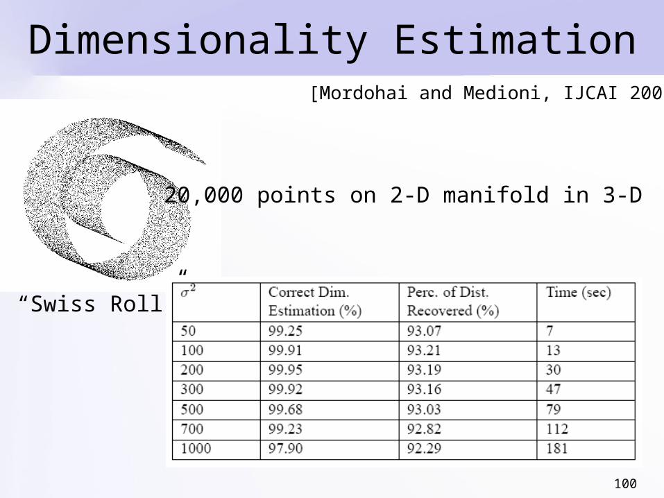
Dimensionality Estimation
“Swiss Roll”
20,000 points on 2-D manifold in 3-D
[Mordohai and Medioni, IJCAI 2005]

101
Dimensionality Estimation• Synthetic data• Randomly sample input variables
(intrinsic dimensionality)• Map them to higher dimensional
vector using linear and quadratic functions
• Add noisy dimensions• Global rotation
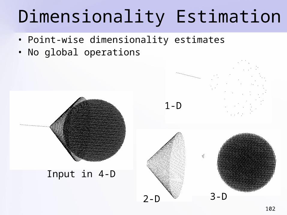
102
Dimensionality Estimation• Point-wise dimensionality estimates• No global operations
Input in 4-D
1-D
3-D2-D
103
Manifold Learning
• Input: instances (points in N-D space)• Try to infer local structure (manifold)
assuming coherence of underlying mechanism that generates instances
• Tensor voting provides:– Dimensionality– Orientation
104
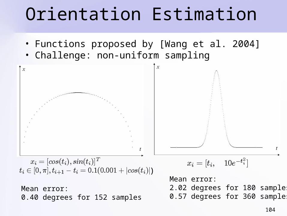
Orientation Estimation
• Functions proposed by [Wang et al. 2004]• Challenge: non-uniform sampling
Mean error: 0.40 degrees for 152 samples
Mean error: 2.02 degrees for 180 samples0.57 degrees for 360 samples
)
105
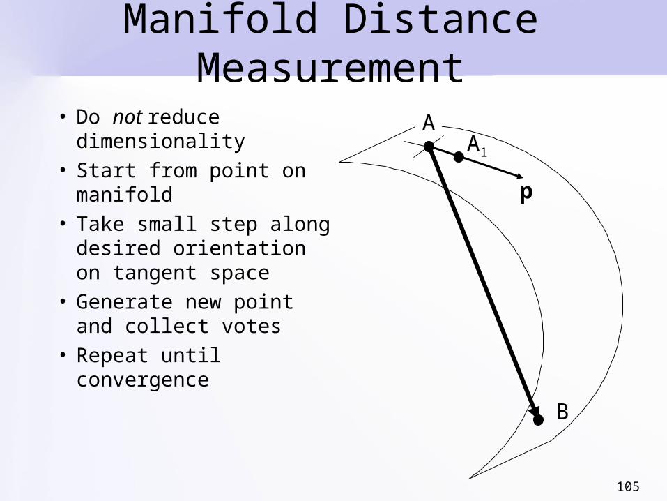
Manifold Distance Measurement
• Do not reduce dimensionality
• Start from point on manifold
• Take small step along desired orientation on tangent space
• Generate new point and collect votes
• Repeat until convergence
AA1
B
p

106
Distance Measurement: Test Data
Error in orientation estimation: 0.11o 0.26o
• Test data: spherical and cylindrical sections– Almost uniformly sampled– Ground truth distances between points are known
• Goal: compare against algorithms that preserve pair-wise properties of being far away or close
107
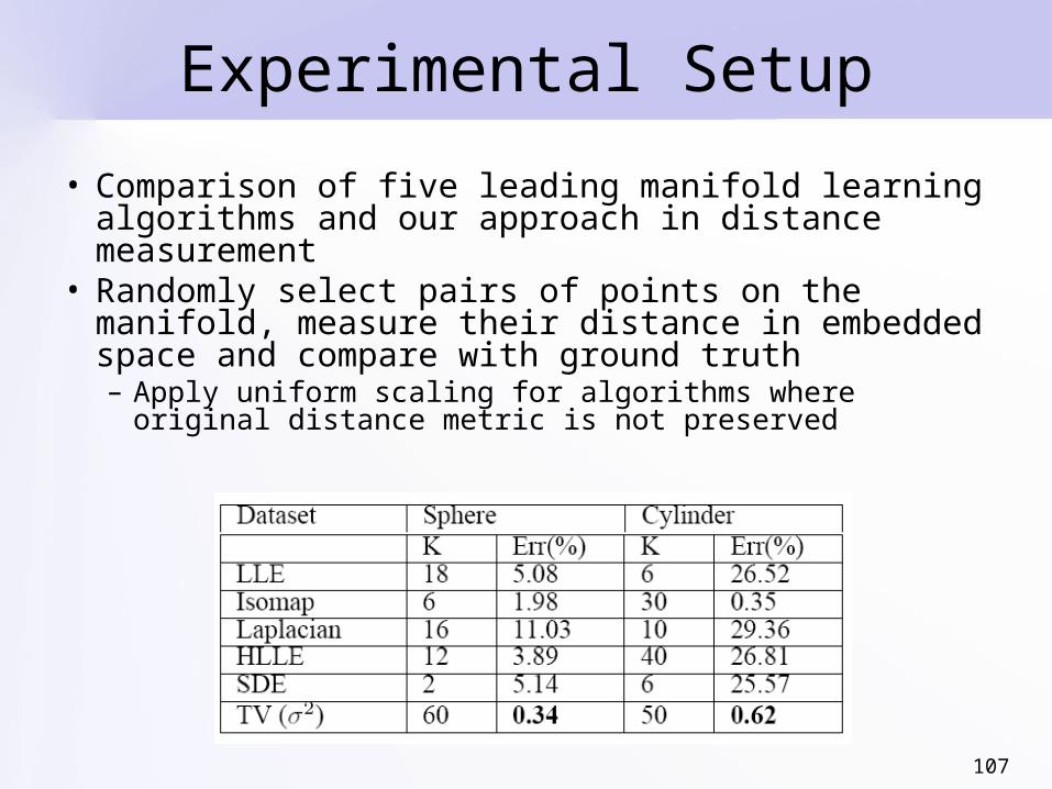
Experimental Setup
• Comparison of five leading manifold learning algorithms and our approach in distance measurement
• Randomly select pairs of points on the manifold, measure their distance in embedded space and compare with ground truth– Apply uniform scaling for algorithms where original
distance metric is not preserved
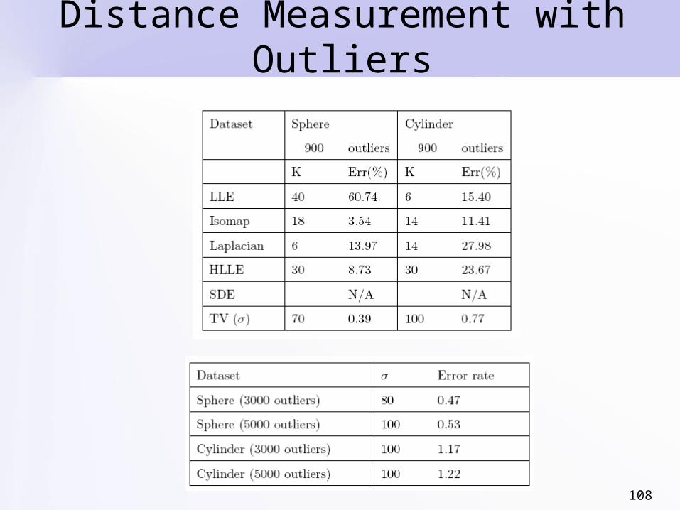
108
Distance Measurement with Outliers

109
Traveling on Manifolds
50-D30-D

110
Function Approximation• Problem: given point Ai in input space predict output value(s)• Find neighbor Bi with known output• Starting from B in joint input-output space, interpolate until A
is reached– A projects on input space within ε of Ai
111
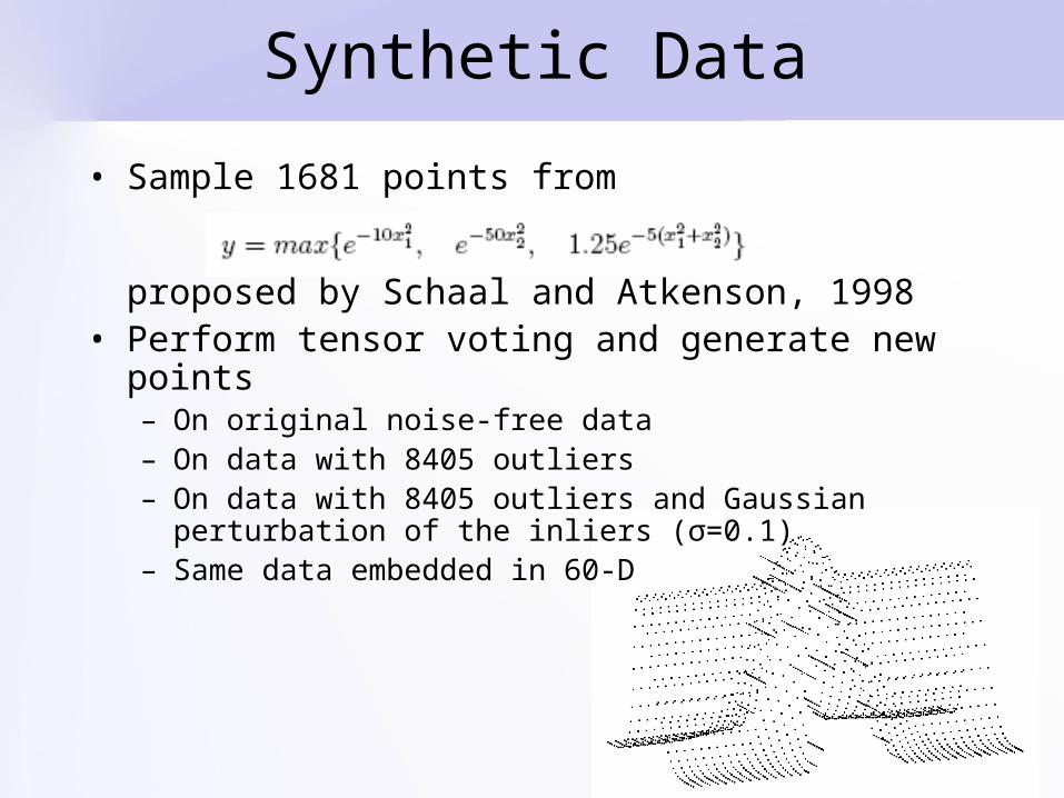
Synthetic Data
• Sample 1681 points from
proposed by Schaal and Atkenson, 1998• Perform tensor voting and generate new points
– On original noise-free data– On data with 8405 outliers– On data with 8405 outliers and Gaussian perturbation
of the inliers (σ=0.1)– Same data embedded in 60-D
112
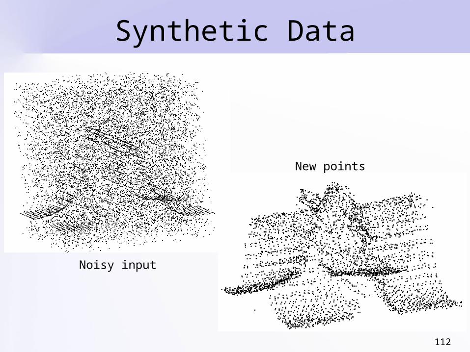
Noisy input
New points
Synthetic Data
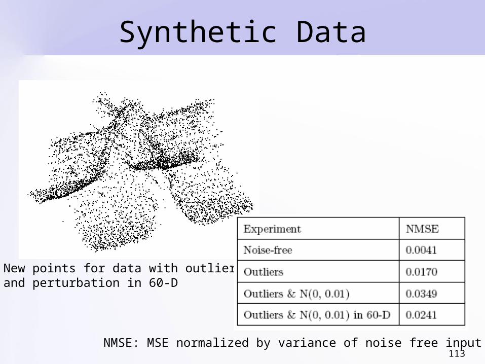
113
New points for data with outliersand perturbation in 60-D
NMSE: MSE normalized by variance of noise free input data
Synthetic Data
114
Function approximation on datasets from:• University of California at Irvine Machine
Learning Repository• DELVE archive
• Rescale data (manually) so that dimensions become comparable (variance 1:10 instead of original 1000:1)
• Split randomly into training and test sets according to literature– Repeat several times
Real Data
115
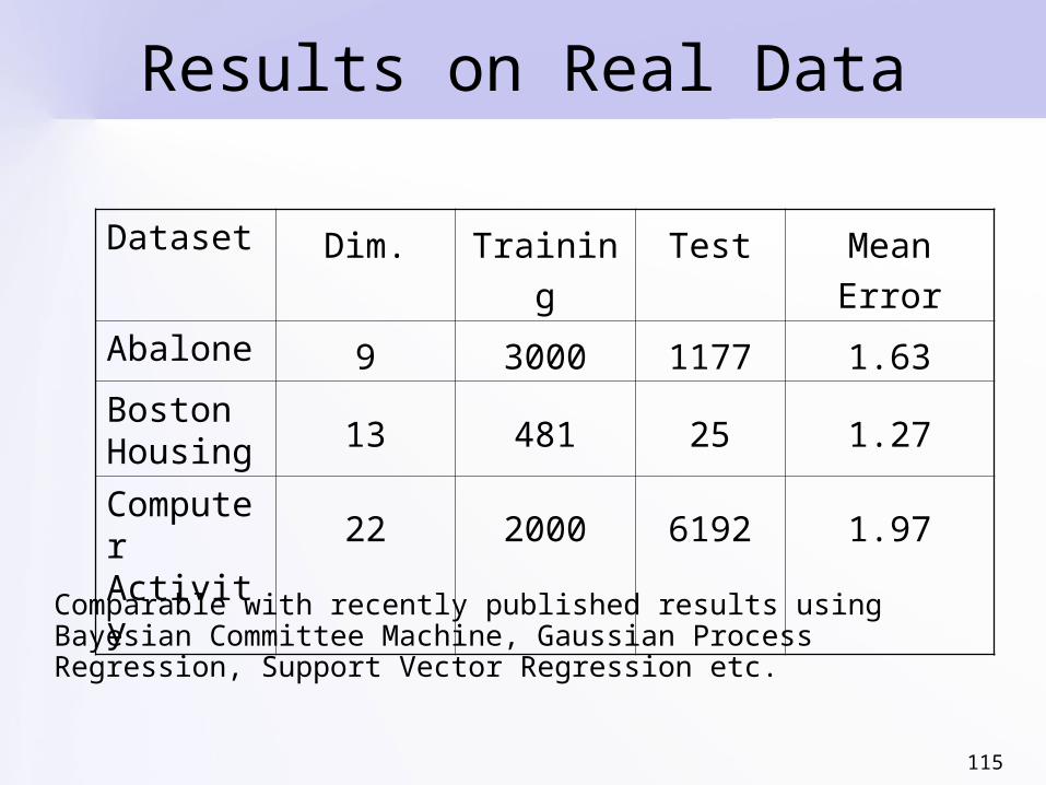
Comparable with recently published results using Bayesian Committee Machine, Gaussian Process Regression, Support Vector Regression etc.
Results on Real Data
Dataset Dim. Training Test Mean Error
Abalone 9 3000 1177 1.63
Boston Housing 13 481 25 1.27
Computer Activity 22 2000 6192 1.97

116
Advantages over State of the Art
• Broader domain for manifold learning– Manifolds with intrinsic curvature (cannot be
unfolded)– Open and closed manifolds (hyper-spheres)– Intersecting manifolds– Data with varying dimensionality
• No global computations O(NM logM)• Noise Robustness
• Limitations:– Need more data– “Regular” distribution

117
Overview
• Introduction• Tensor Voting• Stereo Reconstruction• Tensor Voting in N-D• Machine Learning• Boundary Inference • Figure Completion• More Tensor Voting Research• Conclusions

118
Boundary Inference• Second-order tensors can
represent second order-discontinuities – Discontinuous orientation (A)
• But not first-order discontinuities– Discontinuous structure (C)
Tensor with dominant plate component(orthogonal to surface intersection)
A:A
B
C How to discriminate B from C?
119
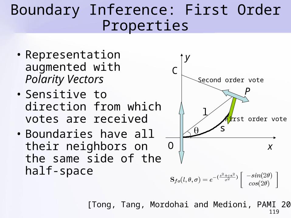
Boundary Inference: First Order Properties
• Representation augmented with Polarity Vectors
• Sensitive to direction from which votes are received
• Boundaries have all their neighbors on the same side of the half-space
x
y
P
s
C
O
l
Second order vote
First order vote
[Tong, Tang, Mordohai and Medioni, PAMI 2004]

120
Illustration of Polarity
Input
Curve Saliency
Polarity

121
Illustration of First Order Voting
Tensor Voting with first order properties

122
Illustration of Region Inference
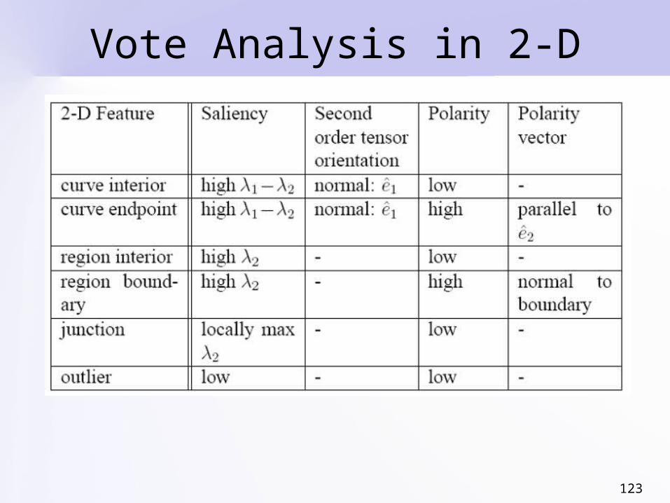
123
Vote Analysis in 2-D
124
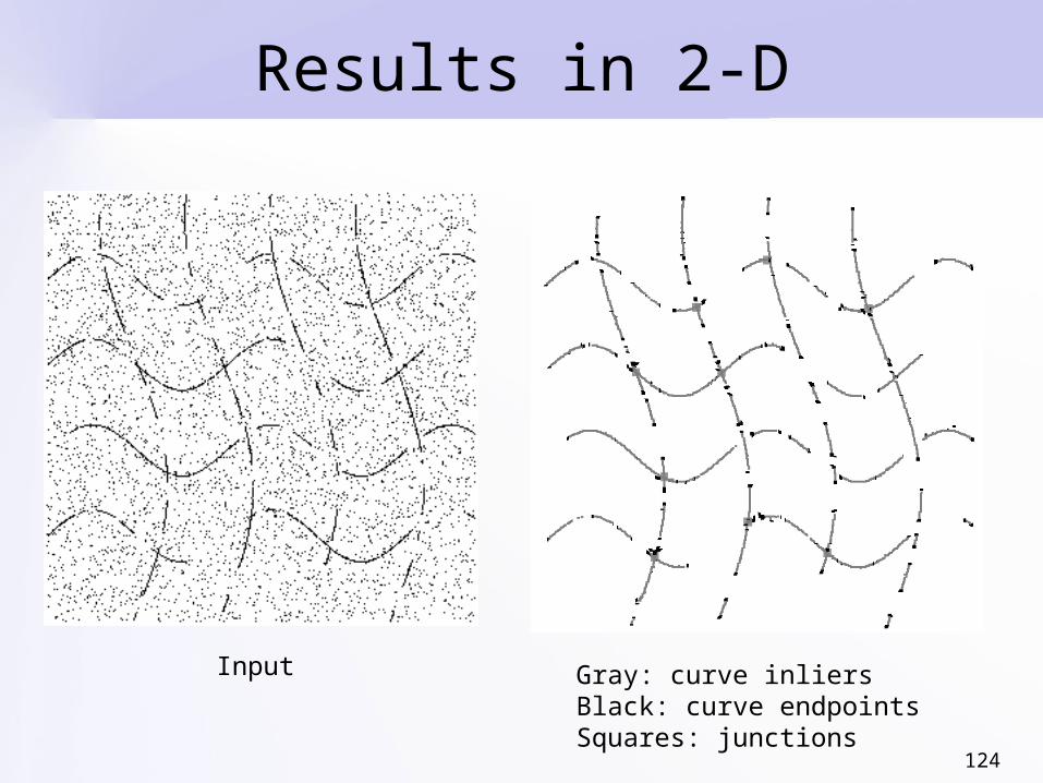
Results in 2-D
Gray: curve inliersBlack: curve endpointsSquares: junctions
Input

125
Results in 2-D
Input Curves and endpoints onlyCurves, endpoints, regions and region boundaries
126
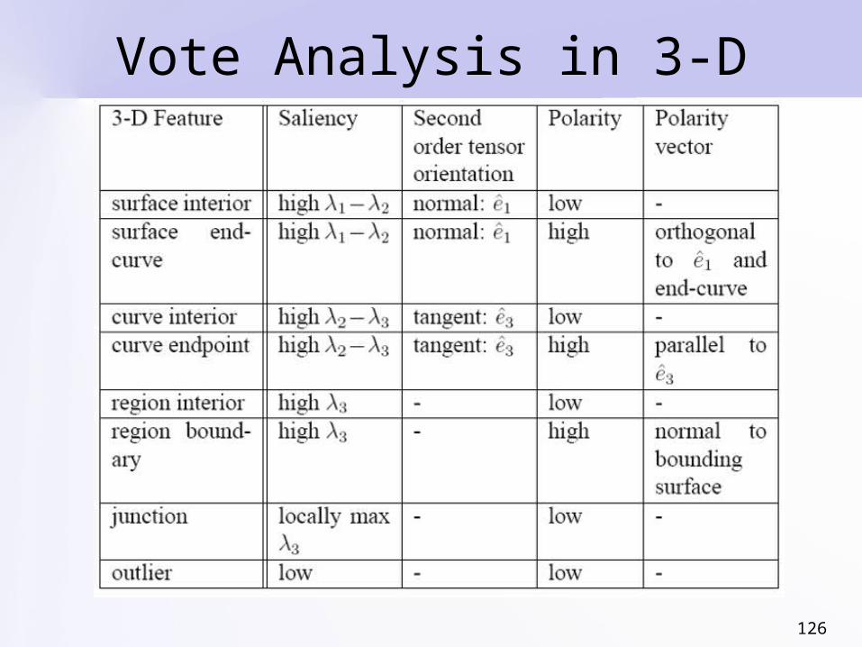
Vote Analysis in 3-D
127
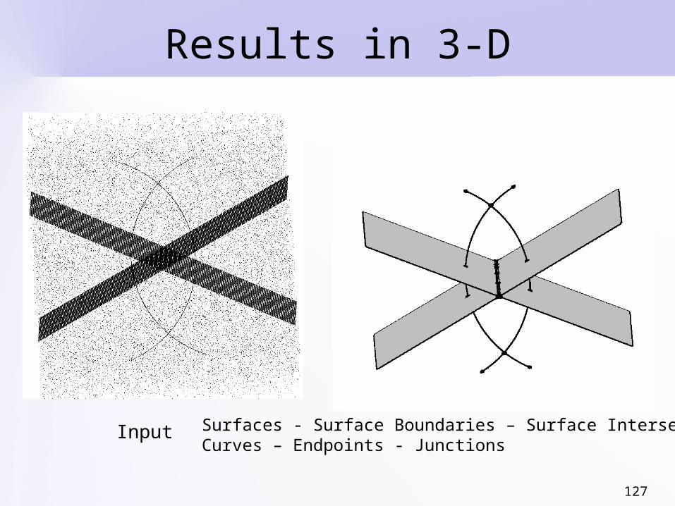
Results in 3-D
Input Surfaces - Surface Boundaries – Surface IntersectionsCurves – Endpoints - Junctions

128
Results in 3-D
Noisy input Dense surface boundary(after marching cubes)

129
Results in 3-D
Input (600k unoriented points) Input with 600k outliers
Output with 1.2M outliers Output with 2.4M outliers
130
Overview
• Introduction• Tensor Voting• Stereo Reconstruction• Tensor Voting in N-D• Machine Learning• Boundary Inference • Figure Completion• More Tensor Voting Research• Conclusions

131
Figure Completion
Amodal completion
Modal completion Layered interpretation
132
Motivation
• Approach for modal and amodal
completion
• Automatic selection between them
• Explanation of challenging visual
stimuli consistent with human
visual system
[Mordohai and Medioni, POCV 2004]

133
Keypoint Detection
• Input binary images• Infer junctions, curves, endpoints,
regions and boundaries• Look for completions supported by
endpoints, L and T-junctions • W, X and Y-junctions do not
support completion by themselves
134
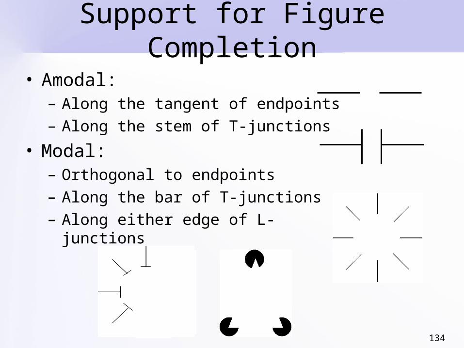
Support for Figure Completion
• Amodal:– Along the tangent of endpoints– Along the stem of T-junctions
• Modal:– Orthogonal to endpoints– Along the bar of T-junctions– Along either edge of L-junctions

135
Voting for Completion
• At least two keypoints of appropriate type needed
• Possible cases:– No possible continuation– Possible amodal completion (parallel
field)– Possible modal completion
(orthogonal field)– If both possibilities available, modal
completion is perceived as occluding amodal one

136
Results: Modal Completion
Input Curves and endpoints Curve saliency Output
137
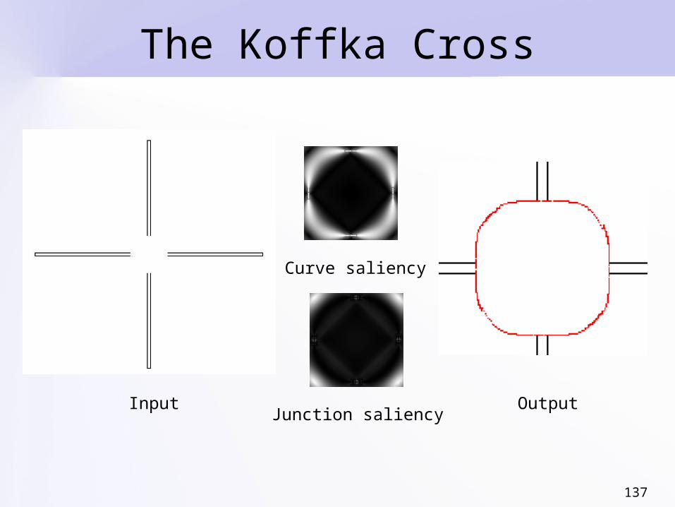
The Koffka Cross
Input
Curve saliency
OutputJunction saliency

138
The Koffka Cross
Input
Curve saliency
OutputJunction saliency
Note: maximum junction saliency here is 90% of maximum curve saliency, but only 10% in the previous case
139
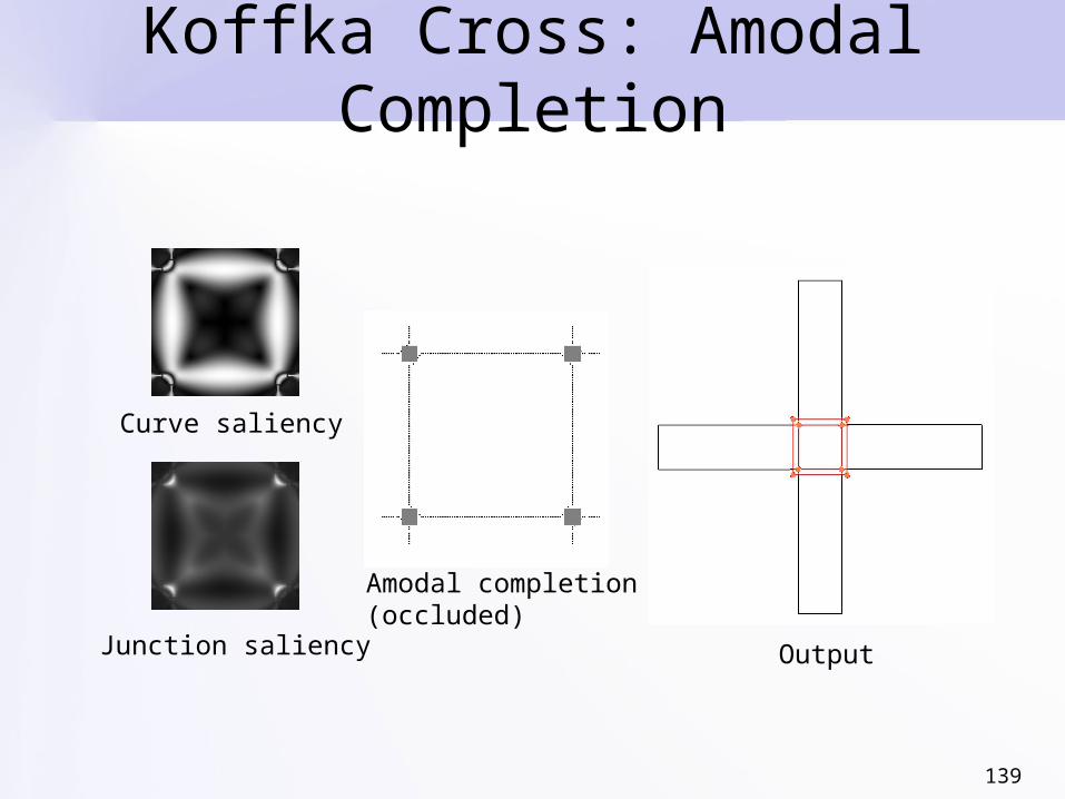
Koffka Cross: Amodal Completion
Curve saliency
OutputJunction saliency
Amodal completion(occluded)
140
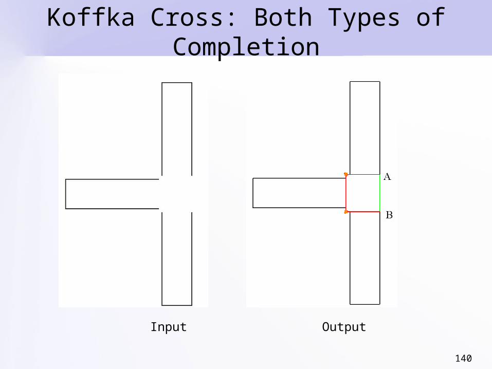
Koffka Cross: Both Types of Completion
Input Output
141
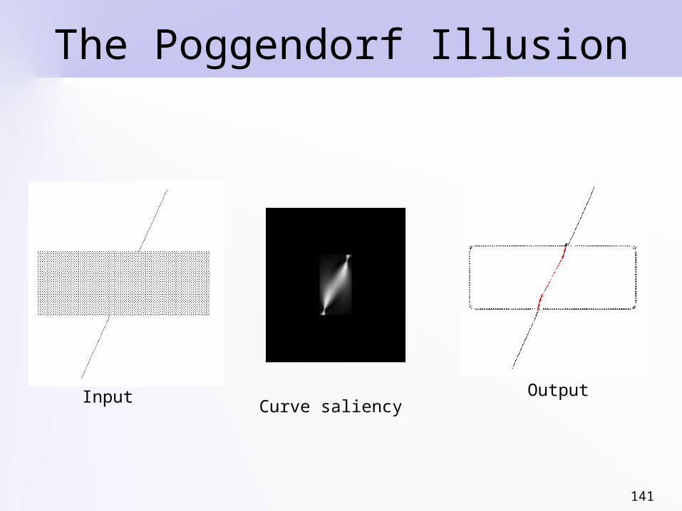
The Poggendorf Illusion
Input OutputCurve saliency

142
The Poggendorf Illusion
Input OutputCurve saliency
143
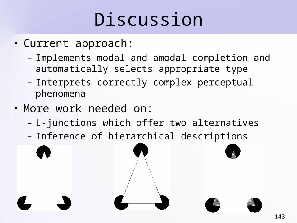
Discussion• Current approach:
– Implements modal and amodal completion and automatically selects appropriate type
– Interprets correctly complex perceptual phenomena
• More work needed on:– L-junctions which offer two alternatives– Inference of hierarchical descriptions

144
Overview
• Introduction• Tensor Voting• Stereo Reconstruction• Tensor Voting in N-D• Machine Learning• Boundary Inference • Figure Completion• More Tensor Voting Research• Conclusions

145
More Tensor Voting Research
• Curvature estimation• Visual motion analysis• Epipolar geometry estimation for
non-static scenes• Texture synthesis

146
Curvature Estimation
• Challenging for noisy, irregular point cloud
• Three passes– Estimate surface normals– Compute subvoxel updates for
positions of points– Compute curvature by collecting votes
from 8 directions (45o apart)
• Infer dense surface
[Tong and Tang, PAMI 2005]
147
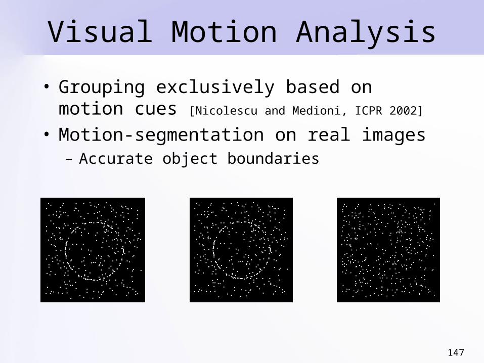
Visual Motion Analysis
• Grouping exclusively based on motion cues [Nicolescu and Medioni, ICPR 2002]
• Motion-segmentation on real images– Accurate object boundaries
148
Visual Motion Analysis
• Potential matches represented by 4-D tensors (x, y, vx, vy)
• Desired motion layers have maximum λ2-λ3
• Results on challenging, non-rigid datasets
149
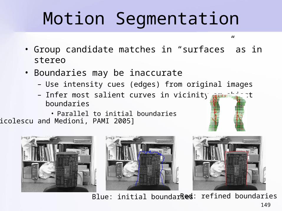
Motion Segmentation
• Group candidate matches in “surfaces” as in stereo
• Boundaries may be inaccurate– Use intensity cues (edges) from original images– Infer most salient curves in vicinity or object boundaries
• Parallel to initial boundaries
Blue: initial boundaries Red: refined boundaries
[Nicolescu and Medioni, PAMI 2005]
150
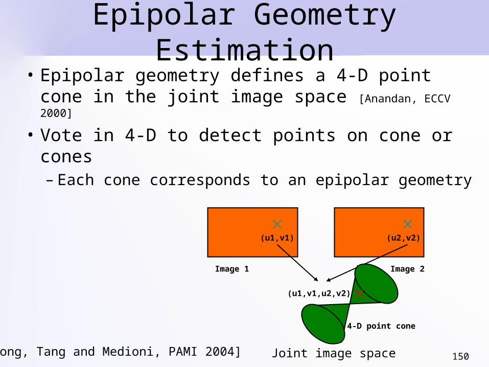
Epipolar Geometry Estimation• Epipolar geometry defines a 4-D point cone
in the joint image space [Anandan, ECCV 2000]
• Vote in 4-D to detect points on cone or cones– Each cone corresponds to an epipolar geometry
(u1,v1) (u2,v2)
(u1,v1,u2,v2)
Image 1 Image 2
4-D point cone
Joint image space[Tong, Tang and Medioni, PAMI 2004]
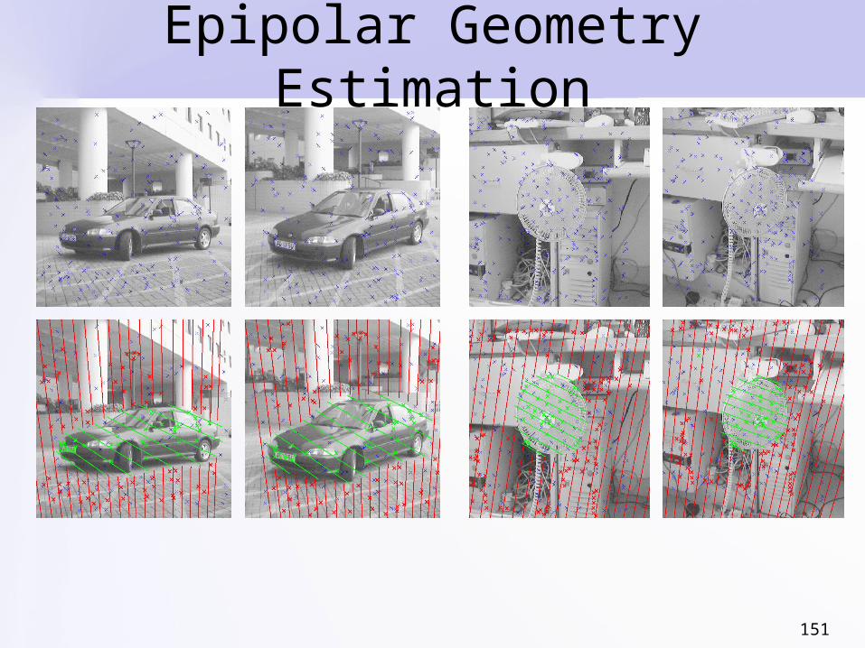
151
Epipolar Geometry Estimation

152
Texture Synthesis
• Given image with user-specified target region• Segment • Connect curves across target region• Synthesize texture via N-D tensor voting
[Jia and Tang, PAMI 2004]

153
Texture Synthesis Results

154
Texture Synthesis Results

155
Overview
• Introduction• Tensor Voting• Stereo Reconstruction• Tensor Voting in N-D• Machine Learning• Boundary Inference • Figure Completion• More Tensor Voting Research• Conclusions
156
Conclusions
• General framework for perceptual organization
• Unified and rich representation for all types of structure, boundaries and intersections
• Model-free
• Applications in several domains

157
Future Work
• Integrated feature detection in real images [Förstner94, Köthe03]– Integrated inference of all feature types (step
and roof edges, all junction types)
• Decision making strategies for interpretation as in [Saund 2003] for binary images and sketches– Symmetry, length, parallelism– Good continuation vs. maximally turning
paths
• Hierarchical descriptions

158
Future Work
• Rich monocular descriptions in terms of:– Shape (invariant as possible)– Occlusion, depth ordering, completion
• Applications– Reconstruction– Recognition
159
Future Work
• Extend manifold learning work– Classification– Complex systems such as forward
and inverse kinematics– Data mining
• Learn from imperfect descriptions– Symbolic not signal-based– Overcome limitations of image-as-
vector-of-pixels representation