1 sliding-mode observers for systems with unknown inputszak/uio_smo_tac.pdf2008/08/22 · 1 2 rm1...

1

Sliding-Mode Observers for Systems With

Unknown Inputs

Karanjit Kalsi†, Jianming Lian†, Stefen Hui‡, Stanislaw H. Zak†

Abstract

The problem of designing sliding-mode observers for systems with unknown inputs is considered

when the so-called observer matching condition is not satisfied. This condition severely restricts the

applicability of sliding-mode observers. To circumvent the observer matching condition, thereby broad-

ening the class of systems for which sliding-mode observers can be constructed, a possible method

is to generate auxiliary outputs that are then used to construct the sliding-mode observer. High-order

sliding-mode exact differentiators can be used to obtain auxiliary outputs. A proof of the asymptotic

stability of the state estimation error is provided. However, the resulting overall observer architecture

is complex. In this paper, high-gain approximate differentiators are proposed to generate the estimates

of auxiliary outputs instead. The resulting architecture is much simpler than the architecture involving

high-order sliding-mode exact differentiators. It is shown that the state estimation error is uniformly

ultimately bounded with respect to a ball whose radius can be controlled by design parameters. The

performance of the high-gain approximate differentiator based sliding-mode observer is demonstrated

to be comparable to that of the observer that uses high-order sliding-mode exact differentiators. The

use of the presented observers to reconstruct the unknown inputs is also analyzed and then illustrated

by numerical examples.

Keywords: Sliding-mode observer, high-order sliding-mode exact differentiator, high-gain approximate

differentiator, unknown input reconstruction.

I. INTRODUCTION

Observers are dynamical systems that can be used to estimate the state of a plant using

its input-output measurements; they were first proposed by Luenberger [1]. In some cases, the

† School of Electrical and Computer Engineering, Purdue University, West Lafayette, IN 47907.‡ Department of Mathematical Sciences, San Diego State University, San Diego, CA 92182.

August 22, 2008 DRAFT

2

inputs to the plant are unknown or partially known, which led to the development of the so-called

unknown input observer (UIO). Examples of linear UIO architectures that have been developed

for linear system are analyzed in [2]–[8]. For non-linear system with unknown inputs, some

of the UIO architectures can be found in [9]–[11]. Motivated by the design of sliding-mode

controllers, first-order sliding mode based UIOs have been developed, see, for example, [12]–

[17]. The main advantage of using sliding-mode observers over their linear counterparts is that

while in sliding, they are insensitive to the unknown inputs and, moreover, they can be used to

reconstruct unknown inputs which could be a combination of system disturbances, faults or non-

linearities. The reconstruction of unknown inputs has found useful applications in fault-detection

and isolation [8], [15], [16].

In most of the linear and non-linear unknown input observers proposed thus far, the necessary

and sufficient conditions for the construction of such observers is that the invariant zeros of the

system must lie in the open left half complex plane, and the transfer function matrix between

unknown inputs and measurable outputs satisfies the observer matching condition. However,

the second condition seriously limits the applicability of this technique. Recently, high-order

sliding mode based unknown input observers [11], [18]–[21] have been developed for systems

that do not satisfy the observer matching condition. In [20], a suitable change of coordinates is

first provided via a constructive algorithm to transform the system into a quasi-block triangular

observable form. Then a step-by-step second order sliding-mode observer is constructed for the

transformed system. In [21], auxiliary outputs are defined such that the conventional unknown

input sliding-mode observer proposed in [15] can be developed for systems without the observer

matching condition. In order to obtain those auxiliary outputs, high-order sliding-mode observers

which act as exact differentiators [22] are constructed based on the super-twisting algorithm

proposed in [23].

In this paper, we adopt the idea of generating auxiliary outputs from [21]. We first incorporate

the high-order sliding-mode observers proposed in [21] into the construction of the sliding-mode

observer which was first introduced in [12] and later modified for a more general class of systems

in [17]. Then we propose a new method of using high-gain observers instead of high-order

sliding-mode observers. High-gain observers are another type of observers for systems with

uncertainties. They were used in [24], [25] to develop output feedback controllers stabilizing

feedback linearizable uncertain systems. The applications of high-gain observers in adaptive


3

control or nonlinear control of uncertain systems can be found in [26], [27]. The incorporation

of high-gain observers into sliding-mode control was initially proposed in [28] and then in [29].

In this paper, high-gain observers are used as approximate differentiators [30] to obtain the

estimates of those auxiliary outputs. The proposed high-gain approximate differentiator based

sliding-mode observer can achieve similar state estimation performance to that of the high-

order sliding-mode exact differentiator based sliding-mode observer. The major advantage of

the proposed high-gain observers over high-order sliding-mode observers used in [21] is the

simplicity of the overall observer architecture. To the best of our knowledge, it is the first time

that the sliding-mode observer presented in [12] is applied to the state observation for linear

systems without the observer matching condition being satisfied. It is also the first time that the

high-gain observer is used in such an application.

The remainder of this paper is organized as follows. The system description and the problem

statement are given in Section II. The sliding-mode exact differentiator is reviewed in Section III,

where it is then incorporated into the sliding-mode observer design. In Section IV, the high-gain

approximate differentiator based sliding-mode observer is proposed and analyzed. Simulation

results using the proposed high-gain approximate differentiator based sliding-mode observer are

included in Section V. Conclusions are in Section VI.

II. SYSTEM DESCRIPTION AND PROBLEM STATEMENT

Let B1 ∈ Rn×m1 , B2 ∈ Rn×m2 and C ∈ Rp×n be known constant matrices, with B2 and

C being of full rank, that is, rank B2 = m2 and rank C = p, and m2 ≤ p. We consider the

following class of linear time-invariant systems with unknown inputs:

x = Ax + B1u1 + B2u2

y = Cx,

(1)

where x ∈ Rn, y ∈ Rp, u1 ∈ Rm1 and u2 ∈ Rm2 are the state, output, known and unknown

input vectors. Let ‖ · ‖ denote the standard Euclidean norm. We assume that there is ρ > 0 such

that ‖u2(t)‖ ≤ ρ for all t. We also assume that the invariant zeros of the system model given

by the triple (A,B2,C) are in the open left-hand complex plane, or equivalently,

rank

sIn −A B2

C Op×m2

= n + m2. (2)


4

Fig. 1. Diagram of the sliding-mode observer.

for all s such that <(s) ≥ 0.

For the system modeled by (1), if the observer matching condition [20] is satisfied, that is,

rank B2 = rank(CB2) = m2, (3)

we can construct the following sliding-mode observer first proposed in [12],

˙x = Ax + B1u1 + L (y − y)−B2E(y, y, η) (4)

with y = Cx and

E(y, y, η) =

ηF (y−y)‖F (y−y)‖ if F (y − y) 6= 0

0 if F (y − y) = 0,(5)

where η is a positive design parameter, L ∈ Rn×p and F ∈ Rm2×p are matrices such that

(A−LC)> P + P (A−LC) = −2Q < 0

and

FC = B>2 P

for some symmetric positive definite P ∈ Rn×n and Q ∈ Rn×n. The architecture of the above

sliding-mode observer is illustrated in Fig. 1. A design algorithm that is adapted from [17] is

summarized in Appendix A.

However, the observer matching condition (3) is sometimes too restrictive for the practical

applications of the above observer. Many physical systems that can be modeled by (1) do not


5

satisfy the observer matching condition (3). In the following, we first construct a sliding-mode

observer for the systems for which the observer matching condition does not hold. We do

this by incorporating sliding-mode exact differentiators proposed in [21]. Then we use high-

gain approximate differentiators that have similar performance but have lower implementation

complexity than sliding-mode exact differentiators.

III. SLIDING-MODE EXACT DIFFERENTIATOR

In this section, we incorporate the sliding-mode exact differentiator proposed in [21] into the

sliding-mode observer design presented in Section II to relax the restriction imposed by the

observer matching condition (3).

A. Auxiliary Output Signal Generation

We first describe the sliding-mode exact differentiators that are used in [21] to generate

auxiliary outputs. Let ci be the i-th row of the output matrix C. Recall that the relative degree

of the i-th output yi with respect to the unknown input u2 is defined to be the smallest positive

integer ri such that

ciAkB2 = 0, k = 0, . . . , ri − 2

ciAri−1B2 6= 0.

We can choose integers γi (1 ≤ γi ≤ ri) such that

Ca =

c1

...

c1Aγ1−1

...

cp

...

cpAγp−1

is of full rank with rank(CaB2) = rank B2. It is proved in [21] that the system zeros of the

system model given by the triple (A, B2,Ca) are in the open left-hand complex plane if the


6

triple (A, B2,C) satisfies (2). Thus, we can construct the sliding-mode observer of the form (4)

for the following system model

x = Ax + B1u1 + B2u2

ya = Cax,

if the output ya = Cax is available. However, the auxiliary outputs in ya are not measurable

and additional observers are required to estimate them.

To proceed, let

yij = ciAj−1x, i = 1, . . . , p, j = 1, . . . , γi. (6)

Thus, we have ya = [y>a1 · · ·y>ap]>, where yai = [yi1 · · · yiγi

]>. The dynamics of yij , j =

1, . . . , γi − 1, are given by

yi1 = yi2 + ciB1u1

...

yi(γi−2) = yi(γi−1) + ciAγi−3B1u1

yi(γi−1) = ciAγi−1x + ciA

γi−2B1u1,

(7)

where x and u1 can be viewed, respectively, as unknown input and known input vectors. We

assume as in [21] that x and x are bounded and

|yij| ≤ dij, i = 1, . . . , p and j = 1, . . . , γi, (8)

which implies that u1 is bounded. Let ν(·), the injection term, be defined by the following super

twisting algorithm [22],ν(·) = φ(·) + λ| · | 12 sign(·)φ(·) = α sign(·),

where λ and α are positive design parameters. For the system (7), which has triangular input

observable form [31], a second-order sliding-mode observer can be constructed as follows:

˙yi1 = ν(yi1 − yi1) + ciB1u1

˙yi2 = Ei1ν(yi2 − yi2) + ciAB1u1

...˙yi(γi−1) = Ei(γi−2)ν

(yi(γi−1) − yi(γi−1)

)+ ciA

γi−2B1u1,

(9)


7

where yi1 = yi1 and yij = ν(yi(j−1) − yi(j−1)), j = 2, . . . , γi − 1, and Eij , j = 1, . . . , γi − 2, are

defined as

Eij =

1 if |yik − yik| = 0 for all k < j

0 otherwise.

Let yij = yij − yij . It follows from (7) and (9) that

˙yi1 = yi2 − ν(yi1 − yi1)

˙yi2 = yi3 − Ei1ν(yi2 − yi2)...

˙yi(γi−2) = yi(γi−1) − Ei(γi−3)ν(yi(γi−2) − yi(γi−2)

)

˙yi(γi−1) = ciAγi−1x− Ei(γi−2)ν

(yi(γi−1) − yi(γi−1)

).

(10)

By choosing sufficiently large λ and α, (see [20]), the system (10) enters sliding mode on the

manifold yi1 = · · · = yi(γi−1) = 0 after a finite time Ti > 0, which implies that

˙yi1 = · · · = ˙yi(γi−1) = 0. (11)

Thus, it follows from (6), (10) and (11) that

ν(yi1 − yi1) = ciAx

ν(yi2 − yi2) = ciA2x

...

ν(yi(γi−1) − yi(γi−1)

)= ciA

γi−1x.

(12)

Let ys = [y>s1 · · · y>sp]> with

ysi =

yi1

ν(yi1 − yi1)

ν(yi2 − yi2)...

ν(yi(γi−1) − yi(γi−1)

)

. (13)

It follows from (12) and (13) that ys = Cax, that is, ys = ya after a finite time T = max1≤i≤p Ti.

Then, in [21], the signal ys derived from the sliding-mode exactor differentiators, described

by (9), is directly used to construct a sliding-mode observer presented in [15]. However, the

transient response of the constructed sliding-mode observer during the time interval [t0, t0 +T ],

where t0 is the initial time, is not analyzed. In the following subsection, we apply the above

sliding-mode exact differentiators to construct the sliding-mode observer.


8

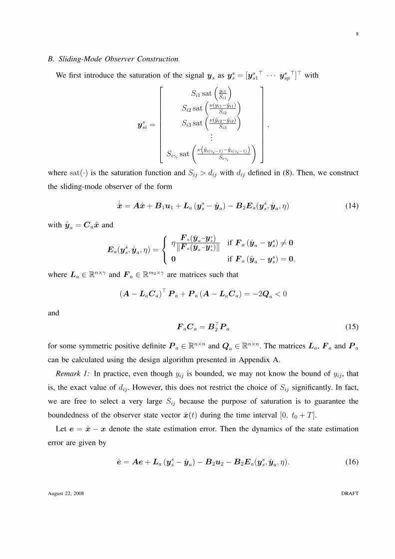
B. Sliding-Mode Observer Construction

We first introduce the saturation of the signal ys as yss = [ys

s1> · · · ys

sp>]> with

yssi =

Si1 sat(

yi1

Si1

)

Si2 sat(

ν(yi1−yi1)Si2

)

Si3 sat(

ν(yi2−yi2)Si3

)

...

Siγisat

(ν(yi(γi−1)−yi(γi−1))

Siγi

)

,

where sat(·) is the saturation function and Sij > dij with dij defined in (8). Then, we construct

the sliding-mode observer of the form

˙x = Ax + B1u1 + La (yss − ya)−B2Ea(y

ss, ya, η) (14)

with ya = Cax and

Ea(yss, ya, η) =

ηF a(ya−ys

s)‖F a(ya−ys

s)‖ if F a (ya − yss) 6= 0

0 if F a (ya − yss) = 0,

where La ∈ Rn×γ and F a ∈ Rm2×γ are matrices such that

(A−LaCa)> P a + P a (A−LaCa) = −2Qa < 0

and

F aCa = B>2 P a (15)

for some symmetric positive definite P a ∈ Rn×n and Qa ∈ Rn×n. The matrices La, F a and P a

can be calculated using the design algorithm presented in Appendix A.

Remark 1: In practice, even though yij is bounded, we may not know the bound of yij , that

is, the exact value of dij . However, this does not restrict the choice of Sij significantly. In fact,

we are free to select a very large Sij because the purpose of saturation is to guarantee the

boundedness of the observer state vector x(t) during the time interval [0, t0 + T ].

Let e = x − x denote the state estimation error. Then the dynamics of the state estimation

error are given by

e = Ae + La (yss − ya)−B2u2 −B2Ea(y

ss, ya, η). (16)


9

In the following, we analyze the performance of the sliding-mode exact differentiator based

sliding-mode observer (14).

Theorem 1: For the dynamical system (1) and the sliding-mode observer (14) with sliding-

mode exact differentiators (9), if η ≥ ρ, then limt→∞ e(t) = 0. Specifically, for any given

positive real R, there exists a finite time Tf (R) such that ‖e(t)‖ ≤ R for t ≥ t0 + Tf (R).

Proof: For t0 ≤ t ≤ t0 + T , it is guaranteed that the observer state vector x(t) in (14) is

bounded because u1, yss and Ea(y

ss, ya, η) are bounded and A − LaCa is Hurwitz. Thus, we

know that e(t) is bounded for t0 ≤ t ≤ t0 + T . For t ≥ t0 + T , we have ys(t) = ya(t) and thus

the dynamics of the state estimation error (16) become

e = Ae + La (ys − ya)−B2u2 −B2Ea(ys, ya, η)

= (A−LaCa) e−B2u2 −B2Ea(ys, ya, η). (17)

Consider the Lyapunov function candidate, V = 12e>P ae for t ≥ t0 + T , where P a is defined

in (III-B). Evaluating the time derivative of V on the solutions of (17), we obtain

V = e>P a (A−LaCa) e− e>P aB2u2 − e>P aB2Ea(ya, ya, η)

= −e>Qae− (F aCae)>u2 − η(F aCae)>Ea(ys, ya, η).

If F aCae = 0, we have

−(F aCae)>u2 − (F aCae)>Ea(ys, ya, η) = 0. (18)

On the other hand, if F aCae 6= 0, we have

−(F aCae)>u2 − (F aCae)>Ea(ys, ya, η)

= −(F aCae)>u2 − η(F aCae)>F aCae

‖F aCae‖≤ −(η − ρ)‖F aCae‖

≤ 0. (19)

It follows from (18) and (19) that in both cases we have

V ≤ −e>Qae ≤ −λmin(Qa)‖e‖2, (20)

which implies that V < 0 and, hence, limt→∞ e(t) = 0.


10

We can rewrite (20) as

V ≤ −λmin(Qa)‖e‖2 ≤ −2µaV, (21)

where µa = λmin(Qa)/λmax(P a). It follows from (21) and the comparison lemma (see, for

example, [32, p. 7] or [33, p. 85]) that

V (t) ≤ exp (−2µa (t− t0 − T )) V (t0 + T ) ,

and thus

‖e(t)‖ ≤ exp (−µa (t− t0 − T ))

√λmax(P a)

λmin(P a)‖e(t0 + T )‖ ,

where e(t0 + T ) is bounded. If√

λmax(P a)/λmin(P a)‖e(t0 + T )‖ > R, then for any given

positive real R, we can find the finite time Tf (R) such that ‖e(t)‖ ≤ R for t ≥ t0 + Tf (R),

where Tf (R) is the solution to the equation

exp (−µa (Tf (R)− T ))

√λmax(P a)

λmin(P a)‖e(t0 + T )‖ = R.

Solving the above gives

Tf (R) = T +1

µa

ln

(√λmin(P a)

λmax(P a)

‖e(t0 + T )‖R

).

On the other hand, if√

λmax(P a)/λmin(P a)‖e(t0 + T )‖ ≤ R, then ‖e(t)‖ ≤ R for t ≥ t0 + T .

In such a case, we can choose Tf (R) = T . Therefore, there exists a finite time Tf (R) such that

‖e(t)‖ ≤ R for t ≥ t0 + Tf (R), which concludes the proof of the theorem.

Corollary 1: For sufficiently large η, the sliding surface: e : σ = F aCae = 0, is invariant

in the state estimation error space and is reached in finite time.

Proof: For a given positive real R, it follows from Theorem 1 that there exists a finite

time Tf (R) such that e(t) is bounded, that is, σ(t) is bounded for t0 ≤ t ≤ t0 + T (R) and

‖e(t)‖ ≤ R for t ≥ t0 + Tf (R). For t ≥ t0 + Tf (R), we obtain, using (15) and (17),

σ>σ = σ> (F aCa(A−LaCa)e− F aCaB2u2 − F aCaB2Ea(ys, ya, η))

≤ ‖F aCa(A−LaCa)‖‖e‖‖σ‖ − σ>(B>2 P aB2)u2 − ησ>(B>

2 P aB2)σ

‖σ‖≤ R‖F aCa(A−LaCa)‖‖σ‖+ λmax(B

>2 P aB2)‖u2‖‖σ‖ − ηλmin(B

>2 P aB2)‖σ‖

≤ −(

η − ρλmax(B>2 P aB2) + R‖F aCa(A−LaCa)‖

λmin(B>2 P aB2)

)λmin(B

>2 P aB2)‖σ‖. (22)


11

The matrix B>2 P aB2 is symmetric positive definite because B2 is of full rank and P a is positive

definite. Therefore, λmin(B>2 P aB2) > 0. If we choose η such that

η ≥ ρλmax(B>2 P aB2) + R‖F aCa(A−LaCa)‖

λmin(B>2 P aB2)

+ ε,

where ε is a small positive constant, then we obtain

σ>σ ≤ −ε‖σ‖, (23)

which implies that e : F aCae = 0 is invariant.

Using the same arguments as in [15, p. 53], we rewrite (23) as

1

2

d

dt‖σ‖2 ≤ −ε‖σ‖. (24)

Integrating (24) from t0 + Tf (R) to t, we obtain

‖σ(t)‖ − ‖σ(t0 + Tf (R))‖ ≤ −ε(t− t0 − Tf (R)).

Let Ts denote the time the sliding surface is reached. We have

‖σ(Ts)‖ − ‖σ(t0 + Tf (R))‖ ≤ −ε(Ts − t0 − Tf (R)),

which implies that

Ts ≤ t0 + Tf (R) +‖σ(t0 + Tf (R))‖

ε.

Thus, the proof of the corollary is complete.

It follows from Corollary 1 that the state estimation error, e, enters sliding mode along e :

σ = 0 after a finite time, and therefore

σ = F aCa (A−LaCa) e− F aCaB2u2 − F aCaB2Ea(yss, ya, η) = 0. (25)

We have limt→∞ e(t) = 0 and then it follows from (25) that as t →∞,

F aCaB2u2 = −F aCaB2Ea(yss, ya, η). (26)

Taking into account (15), we can rewrite (26) as

B>2 P aB2u2 = −B>

2 P aB2Ea(yss, ya, η).

Because B>2 P aB2 is invertible, we obtain

u2 = −Ea(yss, ya, η).

Thus we can estimate the unknown input u2 with increasing accuracy as t →∞.


12

IV. HIGH-GAIN APPROXIMATE DIFFERENTIATOR

Although we can obtain the exact augmented output ya after a finite time by using sliding-

mode exact differentiators, the implementation of second-order sliding-mode observers becomes

complicated for large γi. On the other hand, it is also difficult to choose appropriate λ and α for

the super twisting algorithm. In this section, we propose to use high-gain observers to generate

estimates of those auxiliary outputs in the ya.

A. High-Gain Observer Construction

The dynamics of yai, i = 1, . . . , p, are given by

yi1 = yi2 + ciB1u1

...

yi(γi−1) = yiγi+ ciA

γi−2B1u1

yiγi= fi(x,u2) + ciA

γi−1B1u1,

which can be written as

yai = Aiyai + bi1fi(x, u2) + bi2u1

yi1 = ciyai,

(27)

where the pair (Ai, bi1) is in canonical controllable form which represents the chain of γi

integrators,

fi(x,u2) = ciAγix + ciA

γi−1B1u2, (28)

bi2 = [ciB1 · · · ciAγi−1B1]

> and ci = [1 0 · · · 0]. We also assume for the above system (27)

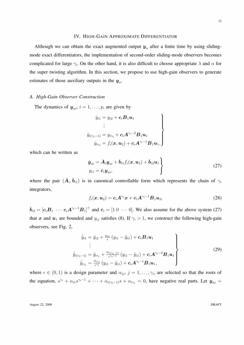
that x and u1 are bounded and yij satisfies (8). If γi > 1, we construct the following high-gain

observers, see Fig. 2,

˙yi1 = yi2 + αi1

ε(yi1 − yi1) + ciB1u1

...˙yi(γi−1) = yiγi

+αi(γi−1)

εγi−1 (yi1 − yi1) + ciAγi−2B1u1

˙yiγi=

αiγi

εγi(yi1 − yi1) + ciA

γi−1B1u1,

(29)

where ε ∈ (0, 1) is a design parameter and αij , j = 1, . . . , γi, are selected so that the roots of

the equation, sγi + αi1sγi−1 + · · · + αi(γi−1)s + αiγi

= 0, have negative real parts. Let yhi =


13

Fig. 2. Diagram of the high-gain observer.

[yi1 · · · yiγi]> and li = [αi1/ε · · · αiγi

/εγi ]>. We can rewrite (29) as

yhi = Aiyhi + lici (yai − yhi) + bi2u1. (30)

If γi = 1, we do not need to construct the above high-gain observer (30) because of the availability

of yi1. In such a case, we have yhi = yai = yi1. To proceed, let ζi = 0 if γi = 1 and let

ζi = [ζi1 · · · ζiγi]> if γi > 1, where

ζij =yij − yij

εγi−j, j = 1, . . . , γi. (31)

It follows from (27) and (30) that

εζi = Aciζi + εbi1fi(x,u2), (32)

where Aci = εD−1i (Ai − lici)Di is a Hurwitz matrix independent of ε.

Proposition 1: For the high-gain observer (30), there exists a finite time Ti(ε) such that

‖ζi(t)‖ ≤ βiε for some positive constant βi and t ≥ t0 + Ti(ε). Moreover, Ti(ε) approaches

zero when ε approaches to zero, that is, limε→0+ Ti(ε) = 0.

Proof: See Appendix B.

It follows from (31) that yai − yhi = Diζi, where Di = diag[εγi−1 εγi−2 · · · 1]. Let yh =

[y>h1 · · · y>hp]>, D = diag[D1 · · · Dp] and ζ = [ζ>1 · · · ζ>p ]>. We have

ya − yh = Dζ. (33)


14

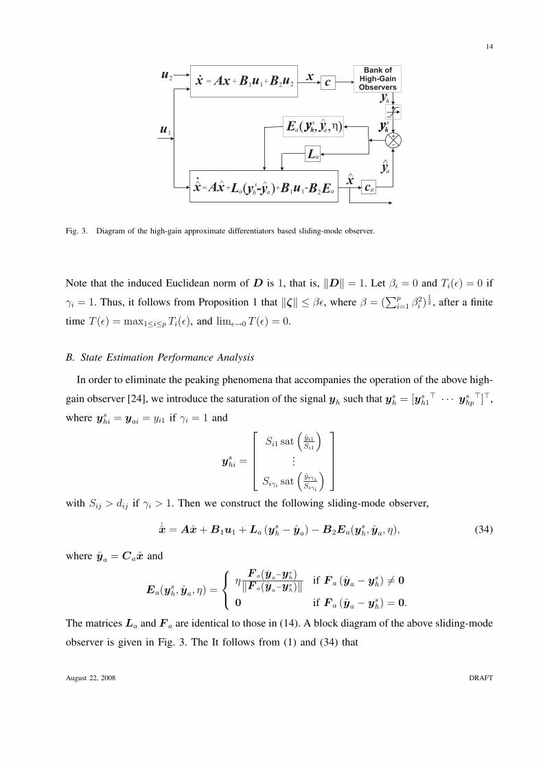
Fig. 3. Diagram of the high-gain approximate differentiators based sliding-mode observer.

Note that the induced Euclidean norm of D is 1, that is, ‖D‖ = 1. Let βi = 0 and Ti(ε) = 0 if

γi = 1. Thus, it follows from Proposition 1 that ‖ζ‖ ≤ βε, where β = (∑p

i=1 β2i )

12 , after a finite

time T (ε) = max1≤i≤p Ti(ε), and limε→0 T (ε) = 0.

B. State Estimation Performance Analysis

In order to eliminate the peaking phenomena that accompanies the operation of the above high-

gain observer [24], we introduce the saturation of the signal yh such that ysh = [ys

h1> · · · ys

hp>]>,

where yshi = yai = yi1 if γi = 1 and

yshi =

Si1 sat(

yi1

Si1

)

...

Siγisat

(yiγi

Siγi

)

with Sij > dij if γi > 1. Then we construct the following sliding-mode observer,

˙x = Ax + B1u1 + La (ysh − ya)−B2Ea(y

sh, ya, η), (34)

where ya = Cax and

Ea(ysh, ya, η) =

ηF a(ya−ys

h)‖F a(ya−ys

h)‖ if F a (ya − ysh) 6= 0

0 if F a (ya − ysh) = 0.

The matrices La and F a are identical to those in (14). A block diagram of the above sliding-mode

observer is given in Fig. 3. The It follows from (1) and (34) that


15

e = Ae + La (ysh − ya)−B2u2 −B2Ea(y

sh, ya, η). (35)

In the following, we analyze the performance of the proposed high-gain approximate differen-

tiator based sliding-mode observer given by (34).

Theorem 2: For the dynamical system (1) and the associated sliding-mode observer (34)

with high-gain approximate differentiators (30), there exists a constant ε∗ ∈ (0, 1) such that

if ε ∈ (0, ε∗) and η ≥ ρ, then the state estimation error e(t) is uniformly ultimately bounded.

Specifically, ‖e(t)‖ ≤ κ(ε) after a finite time Tf (ε), where

κ(ε) =κ1ε +

√κ2

1ε2 + 4µaκ1ε

2µa

√2

λmin(P a)

for positive constants µa, κ1 and κ2.

Proof: It follows from Proposition 1 that ‖ζ(t)‖ ≤ βε for t ≥ t0 + T (ε). Then, it follows

from (33) that ‖ya(t) − yh(t)‖ ≤ βε for t ≥ t0 + T (ε). There exists a constant ε such that if

‖ya(t)− yh(t)‖ ≤ βε, then yh(t) is not saturated, that is, ysh(t) = yh(t). Thus, we can choose

ε∗ = minε, 1 such that if ε ∈ (0, ε∗), then ‖ζ(t)‖ ≤ βε and ysh(t) = yh(t) after a finite time

T (ε).

For t0 ≤ t ≤ t0 + T (ε), it is guaranteed that the observer state vector x(t) in (34) is bounded

because u1, ysh and Ea(y

sh, ya, η) are bounded and A−LaCa is Hurwitz. Thus, e(t) is bounded

for t0 ≤ t ≤ t0 + T (ε). For t ≥ t0 + T (ε), because ysh(t) = yh(t) and yh = ya − Dζ, the

dynamics of the state estimation error (35) become

e = Ae + La (yh − ya)−B2u2 −B2Ea(yh, ya, η)

= Ae + La (ya −Dζ − ya)−B2u2 −B2Ea(yh, ya, η)

= (A−LaCa) e−LaDζ −B2u2 −B2Ea(yh, ya, η). (36)

Consider the Lyapunov function candidate, V = 12e>P ae for t ≥ t0 +T (ε). Evaluating the time

derivative of V on the solutions of (36), we obtain

V = e>P (A−LaCa) e− e>P aLaDζ − e>P aB2u2 − e>P aB2Ea(yh, ya, η)

= −e>Qae− e>P aLaDζ − (F aCae)>u2 − (F aCae)>Ea(yh, ya, η)

= −e>Qae− e>P aLaDζ − (F aCae + FDζ − F aDζ)>u2

− (F aCae + F aDζ − F aDζ)>Ea(yh, ya, η)


16

= −e>Qae− e>P aLaDζ + (F aDζ)>u2 + (F aDζ)>Ea(yh, ya, η)

− (F aCae + FDζ)>u2 − (F aCae + F aDζ)>Ea(yh, ya, η).

If F a(Cae + Dζ) = 0, then

−(F aCae + F aDζ)>u2 − (F aCae + F aCae)>Ea(ya, ya, η) = 0. (37)

On the other hand, if F a(Cae + Dζ) 6= 0, then

−(F aCae + F aDζ)>u2 − (F aCae + F aCae)>Ea(ya, ya, η)

= −(F aCae + F aDζ)>u2 − η(F aCae + F aDζ)>F aCae + F aDζ

‖F aCae + F aDζ‖≤ −(η − ρ)‖F aCae + F aDζ‖

≤ 0. (38)

It follows from (37) and (38) that in both cases we have

V ≤ −e>Qae− e>P aLaDζ + (F aDζ)>u2 + (F aDζ)>Ea(yh, ya, η). (39)

Performing some manipulations gives

V ≤ −λmin(Qa)‖e‖2 + ‖P aLa‖‖D‖‖ζ‖‖e‖+ (η + ρ)‖F a‖‖D‖‖ζ‖

≤ −λmin(Qa)‖e‖2 + βε‖P aLa‖‖e‖+ (η + ρ)βε‖F a‖

= −2µaV + κ1ε√

V + κ2ε, (40)

where

κ1 =

√2β‖P aLa‖√λ

max(P a)

and κ2 = (η + ρ)β‖F a‖.

It follows from (40) that

V ≤ −µaV − µaV + κ1ε√

V + κ2ε

= −µaV −(√

V −R−)(√

V −R+

), (41)

where

R− =κ1ε−

√κ2

1ε2 + 4µaκ2ε

2µa

< 0 and R+ =κ1ε +

√κ2

1ε2 + 4µaκ1ε

2µa

> 0.

We conclude from (41) that V < 0 when ‖e‖ > R+. In summary, the state estimation error e

is uniformly ultimately bounded with respect to any closed ball of radius greater than R+.


17

Hence, as long as√

V > R+, that is, for V > R2+, we have

(√V −R−

)(√V −R+

)< 0.

Therefore, if V (t0 + T (ε)) = V (e(t0 + T (ε))) > R2+ and V (t) > R2

+ for t ≥ t0 + Tf (ε), then

V ≤ −µaV , which implies that

V (t) ≤ exp (−µa (t− t0 − T (ε))) V (t0 + T (ε)) .

Thus, we can find a finite time Tf (ε) such that V (t) ≤ R2+ for t ≥ t0 +T (ε), where Tf (ε) is the

solution to the equation

V (t0 + T (ε)) exp (−µa (Tf (ε)− T (ε))) = R2+,

and has the form,

Tf (ε) = T (ε) +1

µa

ln

(V (t0 + T (ε))

R2+

).

On the other hand, if V (t0 + T (ε)) ≤ R2+, then V (t) ≤ R2

+ for t ≥ t0 + T (ε). In such a case,

we can choose Tf (ε) = T (ε). Therefore, there exists a finite time Tf (ε) such that V (t) ≤ R2+

for t ≥ t0 + Tf (ε), which implies ‖e(t)‖ ≤ κ(ε), where

κ(ε) =κ1ε +

√κ2

1ε2 + 4µaκ1ε

2µa

√2

λmin(P a).

The proof of the theorem is complete.

Remark 2: It follows from Theorem 2 that the state estimation error enters the closed ball

e : ‖e‖ ≤ κ(ε) after a finite time Tf (ε). It is easy to verify that

limε→0+

Tf (ε) =

∞ if V (t0) 6= 0

0 if V (t0) = 0,

because limε→0+ T (ε) = 0 and limε→0+ R+ = 0.

Moreover, the radius of the above closed ball can be adjusted by the design parameter ε and

because limε→0+ κ(ε) = 0, the state estimation error e converges to the origin as ε goes to zero.

Corollary 2: The hyperplane, (e, ζ) : σ = F a(Cae + Dζ) = 0, is invariant in the (e, ζ)-

space and is reached in finite time for sufficiently large η.


18

Proof: For t ≥ t0 + Tf (ε), it follows from (36) that

σ>σ = σ>(F aCae + F aDζ

)

= σ>(

F aCa(A−LaCa)e− F aCaLaDζ − F aCaB2u2

− F aCaB2Ea(yh, ya, η) +1

εF aDAcζ + F aDB1f(x,u2)

)

≤ ‖F aCa(A−LaCa)‖‖e‖‖σ‖+ ‖F aCaLa‖‖D‖‖ζ‖‖σ‖+ σ>(B2P aB2)u2

− ησ>(B2P aB2)σ

‖σ‖ +1

ε‖F aAc‖‖D‖‖ζ‖‖σ‖+ ‖F aB1‖‖f(x,u2)‖‖σ‖

≤ κ(ε)‖F aCa(A−LaCa)‖‖σ‖+ βε‖F aCaLa‖‖σ‖+ λmax(B>2 P aB2)‖u2‖‖σ‖

− ηλmin(B>2 P aB2)‖σ‖+ β‖F aAc‖‖σ‖+ β1‖F aB1‖‖σ‖

= −(

η − κ3 + κ4 + κ5 + κ6 + κ7

λmin(B>2 P aB2)

)λmin(B

>2 P aB2)‖σ‖, (42)

where κ3 = κ(ε)‖F aCa(A − LaCa)‖, κ4 = βε‖F aCaLa‖, κ5 = ρλmax(B>2 P aB2), κ6 =

β‖F aAc‖ and κ7 = ‖F aB1‖‖f(x, u2)‖. It follows from (42) that if we choose η such that

η ≥ κ3 + κ4 + κ5 + κ6 + κ7

λmin(B>2 P aB2)

+ ε,

where ε is a small positive constant, then

σ>σ ≤ −ε‖σ‖, (43)

which implies the above hyperplane is invariant. On the other hand, it can be shown that the

sliding surface will be reached in finite time using the same arguments as in the proof of

Corollary 1. This concludes the proof of the corollary.

C. Unknown Input Reconstruction

Our objective in this subsection is to show that we can use the proposed architecture to

estimate the unknown input u2. We will show that

u2 ≈ −Ea(ysh, ya, η), (44)

after a finite time for sufficiently small ε. We proceed as follows. First, by Corollary 2, we note

that the manifold (e, ζ) : σ = 0 is invariant and is reached after a finite time, and therefore

σ = F aCa(A−LaCa)e− F aCaLaDζ − F aCaB2u2

− F aCaB2Ea(ysh, ya, η) + F aDζ = 0. (45)


19

Substituting (15) into (45) and performing simple manipulations, we obtain

u2 = −Ea(ysh, ya, η)+

(B>

2 P aB2

)−1(F aCa(A−LaCa)e− F aCaLaDζ + F aDζ

). (46)

We thenshow that for sufficiently small ε, ‖e(t)‖, ‖ζ(t)‖ and ‖ζ‖ become negligible after a

finite time, which result in (44).

By Proposition 1, we have ‖ζ(t)‖ ≤ βε for t ≥ t0 + T (ε). By Theorem 2, we have ‖e(t)‖ ≤κ(ε) for t ≥ t0 + Tf (ε), where limε→0+ κ(ε) = 0. Thus, it remains to show that, for sufficiently

small ε, ‖ζ(t)‖ becomes negligible after a finite time. In what follows, we perform preliminary

manipulations before formally proceeding with the proof. Recall that ζ = [ζ>1 · · · ζ>p ]>. Thus,

we only need to prove that, for sufficiently small ε, ‖ζi(t)‖, i = 1, . . . , p, becomes negligible

after a finite time. We first rewrite (32) as

ζi(t) =1

εAciζi(t) + bi1fi(x(t),u2(t))

=1

εAciζi(t) + vi(t), (47)

where vi(t) = bi1fi(x(t),u2(t)). Because x(t) and u2(t) are bounded, it follows from (28) that

fi(x(t), u2(t)) is bounded. Thus, vi(t) is a bounded measurable function. It is well known the

the solution to (47) has the form

ζi(t) = exp

(1

εAci(t− t0)

)ζi(t0) +

∫ t

t0

exp

(1

εAci(t− s)

)vi(s)ds. (48)

Performing a change of variables in the integral of (48) by z = (t− s)/ε, we obtain

ζi(t) = exp

(1

εAci(t− t0)

)ζi(t0) + ε

∫ (t−t0)/ε

0

exp(Aciz

)vi(t− εz)dz. (49)

To proceed, two notions regarding the function vi(t) are defined.

Definition 1: A function vi(t) is left-continuous if limε→0+ vi(t− ε) = vi(t) for all t.

Definition 2: A function vi(t) defined on S ⊂ R is weakly uniformly continuous if for

every ν > 0, there exists a δ > 0 such that for each interval Ω ⊂ S with length less than δ,

‖vi(s)− vi(t)‖ < ν for s, t ∈ Ω.

Remark 3: A function with simple jump discontinuities, for example, a square wave, can

always be made left-continuous by changing the function values at the points of discontinuity.

Note that a uniformly continuous function is weakly uniformly continuous. However, a weakly

uniformly continuous function is not necessarily uniformly continuous. The square wave on


20

the complement of its switching points is an example of a function that is weakly uniformly

continuous but not uniformly continuous. If S is connected, then two notions of uniformly

continuity are equivalent.

In the following, we use S1 +S2, where S1, S2 ⊂ R, to denote the set s1 + s2 : s1 ∈ S1, s2 ∈S2. If S1 or S2 is empty, then S1 + S2 is defined to be empty.

Theorem 3: Consider the dynamics given by (47), where Aci is Hurwitz and vi(t) is bounded.

Let J denote the set of points at which vi(t) is discontinuous and let τ > t0 > 0. If vi(t) is

left-continuous, then limε→0+ ζi(t) = 0 for each t > t0 ≥ 0. Moreover, if vi(t) is also weakly

uniformly continuous on [τ, ∞)\J , then the convergence of ζi(t) to 0 as ε → 0+ is uniform

on [τ, ∞)\(J + (0, ξ)) for each ξ > 0. In particular, if vi(t) is uniformly continuous, then the

convergence is uniform on [τ, ∞).

Proof: It follows from (49) that

ζi(t)

ε= exp

(1

εAci(t− t0)

)ζi(t0)

ε+

∫ (t−t0)/ε

0

exp(Aciz

)vi(t− εz)dz. (50)

Note that the matrix Aci is Hurwitz. Let −λ, λ > 0, denote the maximum of the real parts of

its eigenvalues. The first term on the right hand side of (50) satisfies∥∥∥∥exp

(1

εAci(t− t0)

)ζi(t0)

ε

∥∥∥∥ ≤M1

ε‖ζi(t0)‖ exp

(−1

ελ(t− t0)

), (51)

because ∥∥∥∥exp

(1

εAci(t− t0)

)∥∥∥∥ ≤ M1 exp

(−1

ελ(t− t0)

),

for some M1 > 0. Because the initial conditions for the high-gain observers are always bounded,

there exists M2 > 0 such that

‖ζi(t0)‖ ≤M2

εγi−1.

Substituting the above into (51), we obtain∥∥∥∥exp

(1

εAci(t− t0)

)ζi(t0)

ε

∥∥∥∥ ≤M1M2

εγiexp

(−1

ελ(t− t0)

). (52)

By calculus, for each t > t0 ≥ 0, we have

limε→0+

M1M2

εγiexp

(−1

ελ(t− t0)

)= 0,

and thus,

limε→0+

exp

(1

εAci(t− t0)

)ζi(t0)

ε= 0. (53)


21

We next consider the second term on the right hand side of (50). Let

gi(z) = exp(Aciz

)vi(t− εz)I[0, (t−t0)/ε)(z),

where I[0, (t−t0)/ε)(z) denotes the indicator function for the interval [0, (t− t0)/ε). Observer that

for each z ≥ 0, if vi(t) is left-continuous, then

limε→0+

gi(z) = exp(Aciz

)vi(t).

Because vi(t) is bounded, there exists M3 > 0 such that ‖vi(t)‖ ≤ M3 for all t > t0. Thus, for

each z ≥ 0 and ε ∈ (0, 1),

‖gi(z)‖ ≤ M1M3 exp(−λz).

Because λ > 0, the function exp(−λz) is integrable on [0, ∞). Then we can thus apply

Lebesgue’s dominated convergence theorem [34, page 45] (to each component) such that for

each t > t0 ≥ 0,

limε→0+

∫ (t−t0)/ε

0

exp(Aciz

)vi(t− εz)dz = lim

ε→0+

∫ ∞

0

gi(z)dz

=

∫ ∞

0

exp(Aciz

)vi(t)dz

=

(∫ ∞

0

exp(Aciz

)dz

)vi(t)

= A−1ci

(limz→∞

exp(Aciz

)− Iγi

)vi(t)

= −A−1ci vi(t). (54)

We have limz→∞ exp(Aciz

)= 0 because Aci is Hurwitz. Therefore, it follows from (50), (53)

and (54) that

limε→0+

ζi(t)

ε= −A

−1ci vi(t). (55)

Combining (47) and (55), we conclude that

limε→0+

ζi(t) = Aci limε→0+

ζi(t)

ε+ vi(t) = 0

for each t > t0 ≥ 0.

Now we consider the case when vi(t) is also weakly uniformly continues on [τ, ∞)\J .

Let ν > 0 and τ > t0 > 0. We can use (50) to estimate the difference between ζi(t)/ε and

−A−1ci vi(t). For t ≥ τ , it follows from (52) that there exists a constant µ1 ∈ (0, 1) such that∥∥∥∥exp

(1

εAci(t− t0)

)ζi(t0)

ε

∥∥∥∥ ≤ν

2


22

for ε ∈ (0, µ1). We next analyze the difference between the second term on the right hand side

of (50) and −A−1ci vi(t). Let t ≥ τ . Then we have

∥∥∥∥∥∫ (t−t0)/ε

0

exp(Aciz

)vi(t− εz)dz + A

−1ci vi(t)

∥∥∥∥∥

=

∥∥∥∥∥∫ (t−t0)/ε

0

exp(Aciz

)[vi(t− εz)− vi(t)]dz

+

∫ (t−t0)/ε

0

exp(Aciz

)vi(t)dz + A

−1ci vi(t)

∥∥∥∥∥

≤ M1

∫ (t−t0)/ε

0

exp (−λz) ‖vi(t− εz)− vi(t)‖dz

+

∥∥∥∥∥∫ (t−t0)/ε

0

exp(Aciz

)vi(t)dz + A

−1ci vi(t)

∥∥∥∥∥ .

We analyze the terms in the above sum separately.

Let S = [τ, ∞)\(J + (0, ξ)). The set S is closed and it may be empty. For each t ∈ S, the

distance from t to the nearest point of discontinuity less than t is at least ξ since all points with

distance less than ξ to the right of a point of discontinuity are removed. Note that it is possible

for S to contain a point of discontinuity.

Let t ∈ S. By assumption, vi(t) is weakly uniformly continuous on [τ, ∞)\J . Because

(t − ξ, t) ⊂ [τ, ∞)\J , we can choose δ, independent of t, such that 0 < δ < ξ and ‖vi(s) −vi(w)‖ ≤ λν/(8M1) for s, w ∈ (t − δ, t). Because vi(t) is left-continuous, we conclude, by

letting w → t−, that ‖v(s)− v(t)‖ ≤ λν/(8M1) for s ∈ (t− δ, t]. Then we have

M1

∫ (t−t0)/ε

0


= M1

(∫ δ/ε

0

+

∫ (t−t0)/ε

δ/ε


)

<λν

8

∫ δ/ε

0

exp (−λz) dz + 2M1M3

∫ (t−t0)/ε

δ/ε

exp (−λz) dz

<λν

8

∫ ∞

0

exp (−λz) dz + 2M1M3

∫ ∞

δ/ε

exp (−λz) dz

=ν

8+

2M1M3

λexp

(−λδ

ε

).


23

Choose µ2 ∈ (0, 1) such that2M1M3

λexp

(−λδ

ε

)≤ ν

8

for ε ∈ (0, µ2). It follows that for t ∈ S and ε ∈ (0, µ2),

M1

∫ (t−t0)/ε

0

exp (−λz) ‖vi(t− εz)− vi(t)‖dz ≤ ν

4.

On the other hand, we have∥∥∥∥∥∫ (t−t0)/ε

0

exp(Aciz

)vi(t)dz + A

−1ci vi(t)

∥∥∥∥∥

=

∥∥∥∥A−1ci

[exp

(1

εAci(t− t0)

)− Iγi

]vi(t) + A

−1ci vi(t)

∥∥∥∥

=∥∥∥A

−1ci

∥∥∥∥∥∥∥exp

(1

εAci(t− t0)

)vi(t)

∥∥∥∥

≤ M1M3

∥∥∥A−1ci

∥∥∥ exp

(−λ(t− t0)

ε

)

≤ M1M3

∥∥∥A−1ci

∥∥∥ exp

(−λ(τ − t0)

ε

),

because λ > 0, ε > 0 and t ≥ τ . Choose µ3 ∈ (0, 1) such that

M1M3

∥∥∥A−1ci

∥∥∥ exp

(−λ(τ − t0)

ε

)<

ν

4

for ε ∈ (0, µ3). Let µ = minµ1, µ2, µ3. Then, combining the above inequalities, we conclude

that for t ∈ S and ε ∈ (0, µ), ∥∥∥∥ζi(t)

ε+ A

−1ci vi(t)

∥∥∥∥ ≤ ν,

which implies that ζi(t)/ε converges uniformly to −A−1ci vi(t) on S. The uniform convergence

of ζi(t) to 0 on [τ, ∞)\(J + (0, ξ)) follows immediately.

If vi(t) is uniformly continuous, then J is empty which implies that J + (0, ξ) is empty.

Thus, it follows that the convergence of ζi(t) to 0 is uniform on [τ, ∞) and the proof of the

theorem is complete.

The estimation of the unknown inputs illustrated in Section V will show that one cannot expect

uniform convergence in an immediate neighborhood of a jump discontinuity and a small interval

to the right of such a discontinuity must be excised to guarantee uniform convergence. On the

other hand, the above theorem does not hold if the function vi(t) is only weakly uniformly

continuous on [τ, T ]\J or uniformly continuous on [τ, T ] for T > τ . For example, if the


24

unknown input u2(t) contains signals of the form sin(t2), then vi(t) is only uniformly continuous

on [τ, T ] for T > τ . Thus, we have the following local version of Theorem 3.

Corollary 3: Consider the dynamics given by (47), where Aci is Hurwitz and vi(t) is bounded.

Let J denote the set of discontinuities of vi(t) and let 0 < t0 < τ < T . Suppose vi(t) is left-

continuous and weakly uniformly continuous on [τ, T ]\J (or uniformly continuous on [τ, T ]).

Then for each ξ > 0, the convergence of ζi(t) to 0 as ε → 0+ is uniform on [τ, T ]\(J +(0, ξ))

(or [τ, T ]).

V. NUMERICAL EXAMPLES

In this section, we illustrate the effectiveness of our proposed high-gain approximate differen-

tiator based sliding-mode observer with two numerical examples. Our simulations demonstrate

that its performance is quite similar to that of the high-order sliding-mode exact differentiator

based sliding-mode observer. Due to lack of space, we only show simulations with the high-gain

approximate differentiator based sliding-mode observer.

Example 1: We first consider a linear time invariant system (1) determined by

A =

0 1 0 0 0

0 0 1 0 0

0 0 0 1 0

0 0 0 0 1

−1 −5 −10 −10 −5

, B1 = B2 =

0 0

0 0

0 −1

1 0

0 0

,

C =

1 0 0 0 0

0 0 0 1 0

.

The initial condition is x(0) = [0.5 0.5 0.5 −0.5 −0.5]>, and the known input u1 is set to be

zero vector. The unknown input u2 consists of a square wave with amplitude 1 and frequency

1Hz, and a sawtooth signal with amplitude 2 and frequency 1Hz.

It is easy to check that for this system rank(CB2) 6= rank B2 because c1B2 = 0. Thus, we

choose γ1 = r1 = 3 such that

Ca =

c1

c1A

c1A2

c2

=

1 0 0 0 0

0 1 0 0 0

0 0 1 0 0

0 0 0 1 0


25

0 2 4 6 8 10−1.5

−1

−0.5

0

0.5

1

1.5

time (sec)

y12

y12

estimate

0 2 4 6 8 10−1.5

−1

−0.5

0

0.5

1

1.5

time (sec)

y13

y13

estimate

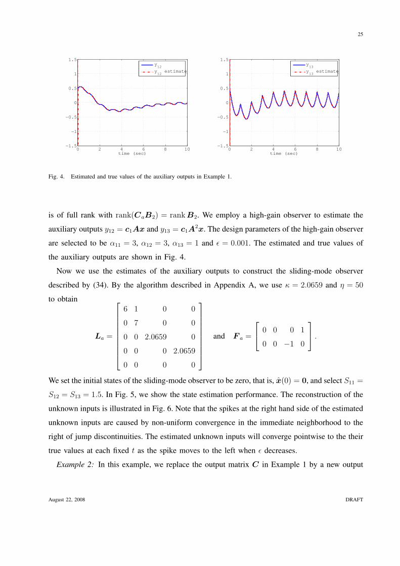
Fig. 4. Estimated and true values of the auxiliary outputs in Example 1.

is of full rank with rank(CaB2) = rank B2. We employ a high-gain observer to estimate the

auxiliary outputs y12 = c1Ax and y13 = c1A2x. The design parameters of the high-gain observer

are selected to be α11 = 3, α12 = 3, α13 = 1 and ε = 0.001. The estimated and true values of

the auxiliary outputs are shown in Fig. 4.

Now we use the estimates of the auxiliary outputs to construct the sliding-mode observer

described by (34). By the algorithm described in Appendix A, we use κ = 2.0659 and η = 50

to obtain

La =

6 1 0 0

0 7 0 0

0 0 2.0659 0

0 0 0 2.0659

0 0 0 0

and F a =

0 0 0 1

0 0 −1 0

.

We set the initial states of the sliding-mode observer to be zero, that is, x(0) = 0, and select S11 =

S12 = S13 = 1.5. In Fig. 5, we show the state estimation performance. The reconstruction of the

unknown inputs is illustrated in Fig. 6. Note that the spikes at the right hand side of the estimated

unknown inputs are caused by non-uniform convergence in the immediate neighborhood to the

right of jump discontinuities. The estimated unknown inputs will converge pointwise to the their

true values at each fixed t as the spike moves to the left when ε decreases.

Example 2: In this example, we replace the output matrix C in Example 1 by a new output


26

0 2 4 6 8 10−0.5

0

0.5

1

1.5

time (sec)

x1

x1 estimate

0 2 4 6 8 10−0.5

0

0.5

1

time (sec)

x2

x2 estimate

0 2 4 6 8 10−1

−0.8

−0.6

−0.4

−0.2

0

0.2

0.4

0.6

0.8

1

time (sec)

x3

x3 estimate

0 2 4 6 8 10−1

−0.8

−0.6

−0.4

−0.2

0

0.2

0.4

0.6

0.8

1

time (sec)

x4

x4 estimate

0 2 4 6 8 10−1.5

−1

−0.5

0

0.5

1

1.5

2

time (sec)

x5

x5 estimate

Fig. 5. Real and estimated system states in Example 1.


27

0 2 4 6 8 10−3

−2

−1

0

1

2

3

time (sec)

u21

u21

estimate

0 2 4 6 8 10−4

−3

−2

−1

0

1

2

3

4

time (sec)

u22

u22

estimate

Fig. 6. Unknown input reconstruction in Example 1.

matrix

C =

2 1 0 0 0

−2 1 0 0 1

.

We keep the same initial condition, known and unknown inputs as in Example 1. With the new

output matrix, we have c1B2 = c2B2 = 0. Thus, we choose γ1 = r1 = 2 and γ2 = r2 = 2 such

that

Ca

c1

c1A

c2

c2A

=

2 1 0 0 0

0 2 1 0 0

−2 1 0 0 1

−1 −7 −9 −10 −5

,

is of full rank with rank(CaB2) = rank B2. We employ two separate high-gain observers to

estimate the auxiliary outputs y12 = c1Ax and y22 = c2Ax, respectively. The design parameters

of high-gain observers are chosen to be α11 = 2, α12 = 1, α21 = 2, α22 = 1 and ε = 0.001. The

estimated and true values of the auxiliary outputs are shown in Fig. 7.

Following the algorithm described in Appendix A with κ = 158.3395 and η = 100, we obtain

La =

1.9276 0 −1.3947 0

2.5626 0 2.2961 0

−5.1252 10 −4.5923 0

2.2264 −9 1.9168 −1

0.7994 0 1.4967 0

and F a =

0 0 0 −10

0 −1 0 9

.


28

0 2 4 6 8 10−1.5

−1

−0.5

0

0.5

1

1.5

time (sec)

y12

y12

estimate

0 2 4 6 8 10−6

−4

−2

0

2

4

6

time (sec)

y2

y2 estimate

Fig. 7. Estimated and true values of the auxiliary outputs in Example 2.

0 2 4 6 8 10−3

−2

−1

0

1

2

3

time (sec)

u21

u21

estimate

0 2 4 6 8 10−4

−3

−2

−1

0

1

2

3

4

time (sec)

u22

u22

estimate

Fig. 8. Unknown input reconstruction in Example 2.

The initial states of the sliding-mode observer is the same as in Example 1, S11 = S12 = S21 = 3

and S22 = 8. The state estimation performance is similar to that of Example 1 as shown in Fig. 5.

The reconstruction of the unknown inputs is illustrated in Fig. 8.

VI. CONCLUSIONS

The main contributions of this paper are novel sliding-mode observer architectures for state

estimation and unknown input reconstruction for systems with unknown inputs. Rigorous proofs

of the convergence of the state estimation error and the unknown input reconstruction are

provided. The proposed architectures consist of dynamical systems for generating auxiliary


29

outputs that are used by a sliding-mode observer to estimate the states and reconstruct the

unknown inputs. Two methods for generating auxiliary outputs are analyzed: high-order sliding-

mode exact differentiator and high-gain approximate differentiator. The first method yields

asymptotic state estimation, whereas the second method achieves uniform ultimate boundedness

of the state estimation error. The high-gain approximate differentiators result in a simpler overall

observer architecture than the high-order sliding-mode exact differentiator. In addition, it is

shown that the high-gain differentiator based observer performs comparably to the high-order

differentiator based observer.

APPENDIX A

SLIDING-MODE OBSERVER DESIGN ALGORITHM

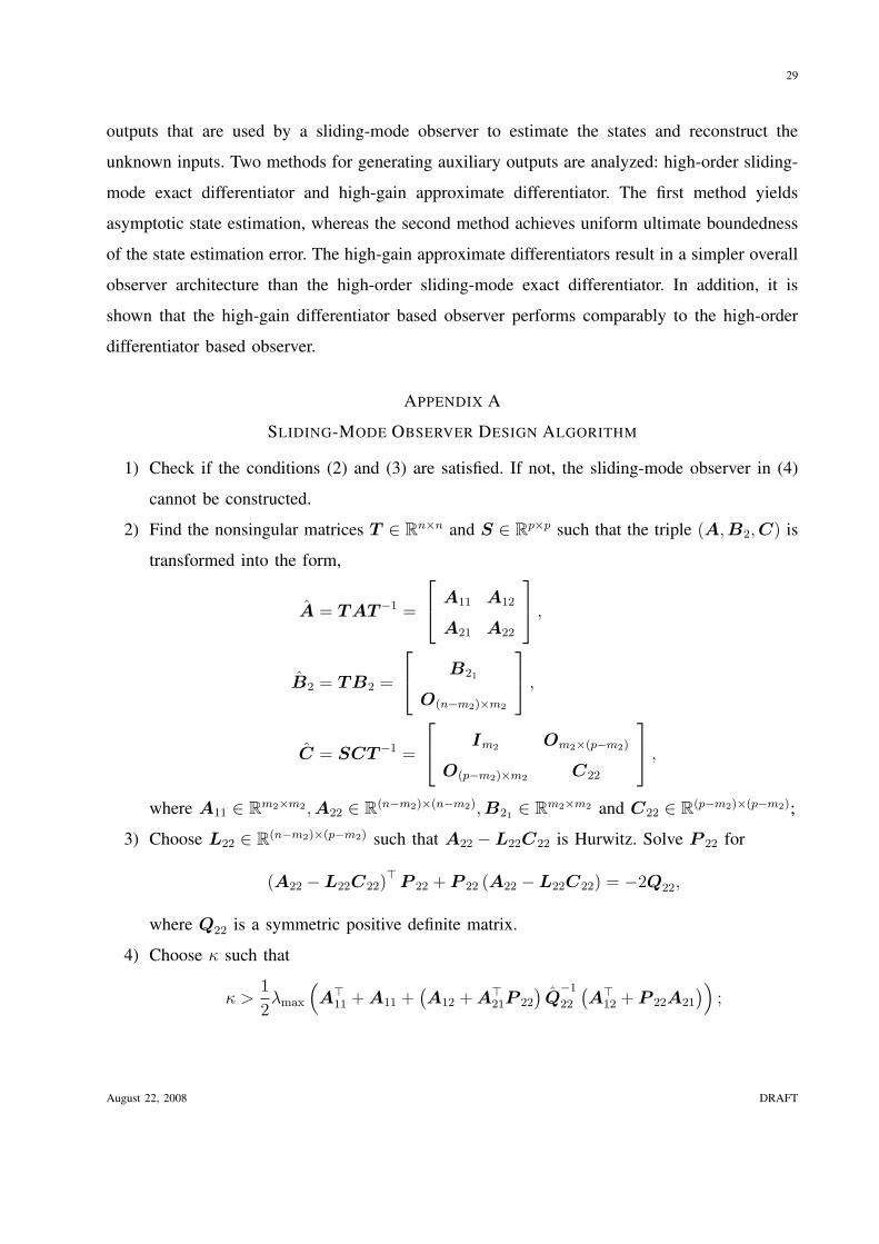
1) Check if the conditions (2) and (3) are satisfied. If not, the sliding-mode observer in (4)

cannot be constructed.

2) Find the nonsingular matrices T ∈ Rn×n and S ∈ Rp×p such that the triple (A,B2,C) is

transformed into the form,

A = TAT−1 =

A11 A12

A21 A22

,

B2 = TB2 =

B21

O(n−m2)×m2

,

C = SCT−1 =

Im2 Om2×(p−m2)

O(p−m2)×m2 C22

,

where A11 ∈ Rm2×m2 , A22 ∈ R(n−m2)×(n−m2), B21 ∈ Rm2×m2 and C22 ∈ R(p−m2)×(p−m2);

3) Choose L22 ∈ R(n−m2)×(p−m2) such that A22 −L22C22 is Hurwitz. Solve P 22 for

(A22 −L22C22)> P 22 + P 22 (A22 −L22C22) = −2Q22,

where Q22 is a symmetric positive definite matrix.

4) Choose κ such that

κ >1

2λmax

(A>

11 + A11 +(A12 + A>

21P 22

)Q−1

22

(A>

12 + P 22A21

));


30

5) Construct P , F and L as

P =

Im2 Om2×(p−m2)

O(p−m2)×m2 P 22

,

F =[

B>21

Om2×(p−m2)

],

L =

κIm2 Om2×(p−m2)

O(n−m2)×m2 L22

,

and compute P = T>P T , F = F S, L = T−1LS;

6) Construct the sliding-mode observer (4).

APPENDIX B

PROOF OF PROPOSITION 1

The idea of this proof comes from [35]. Let P ci be the solution to the continuous Lyapunov

equation A>ciP ci + P ciAci = −2Qci for some Qci = Q>

ci > 0. Consider the Lyapunov function

candidate for t ≥ t0,

Vi =1

2ζ>i P ciζi. (56)

Evaluating the time derivative of Vi on the solutions of (32), yields

Vi = ζ>i P ci

(1

εAciζi + bi1fi(x,u2)

)

≤ −1

εζ>i Qciζi +

∥∥ζ>i P cibi1

∥∥ |fi(x,u2)| . (57)

Because x and u2 are bounded, it follows from (28) that |fi(x,u2)| ≤ βi1 for some βi1 > 0.

Taking into account the above and performing some manipulations on (57) gives

Vi = −1

εζ>i Qciζi + βi1

∥∥ζ>i P cibi1

∥∥

≤ −1

ελmin(Qci)‖ζi‖2 + βi1‖P cibi1‖‖ζi‖

≤ −1

ε

λmin(Qci)

λmax(P ci)λmax(P ci)‖ζi‖2 +

√2βi1‖P cibi1‖√

λmin(P ci)

√1

2λmin(P ci)‖ζi‖2

≤ −21

ε

λmin(Qci)

λmax(P ci)Vi +


λmin(P ci)

√Vi

= −µci

εVi −

√Vi

(µci

ε

√Vi − βi2

),


31

where

µci =λmin(Qci)

λmax(P ci), βi2 =


λmin(P ci).

It is easy to verify that as long as

Vi ≥(

βi2ε

µci

)2

= βi3ε2,

where βi3 = β2i2/µ

2ci, then

µci

ε

√Vi − βi2 ≥ 0.

Because the initial conditions for the high-gain observers are bounded and ε is a design parameter

such that 0 < ε < 1, it follows from (56) that

Vi(t0) ≤ βi4

ε2γi−2,

for some βi4 > 0.

If Vi(t0) > βi3ε2 and Vi(t) ≥ βi3ε

2 for t ≥ t0, then

Vi ≤ −µci

εVi,

and, hence, it follows from the comparison lemma that

Vi(t) ≤ exp(−µci

ε(t− t0)

)Vi(t0) ≤ βi4

ε2γi−2

(−µci

ε(t− t0)

).

Thus, we can find a finite time Ti(ε) such that Vi(t) ≤ βi3ε2 for t ≥ t0 + Ti(ε), where Ti(ε) is

the solution to the equation,

βi4

ε2γi−2exp

(−µci

εTi(ε)

)= βi3ε

2,

of the form,

Ti(ε) =ε

µci

ln

(βi4

βi3ε2γi

). (58)

It follows from (58) that limε→0+ Ti(ε) = 0. On the other hand, if Vi(t0) ≤ βi3ε2, then Vi(t) ≤

βi3ε2 for t ≥ t0. In such a case, we can choose Ti(ε) = 0. Therefore, there exists a finite

time Ti(ε) such that Vi(t) ≤ βi3ε2 for t ≥ t0 + Ti(ε) and limε→0+ Ti(ε) = 0. It follows that

‖ζ(t)‖ ≤ βiε for t ≥ t0 + Ti(ε), where βi =√

2βi3/λmin(P ci). Thus, we concludes the proof of

the proposition.


32

REFERENCES

[1] D. G. Luenberger, “Observers for multivariable systems,” IEEE Trans. Autom. Control, vol. AC-11, no. 2, pp. 190–197,

Apr. 1966.

[2] S. P. Bhattacharyya, “Observers design for linear systems with unknown inputs,” IEEE Trans. Autom. Control, vol. AC-23,

no. 3, pp. 483–484, Jun. 1978.

[3] P. Kudva, N. Viswanadham, and A. Ramakrishna, “Observers for linear systems with unknown inputs,” IEEE Trans. Autom.

Control, vol. AC-25, no. 1, pp. 113–115, Feb. 1980.

[4] F. Yang and R. W. Wilde, “Observers for linear systems with unknown inputs,” IEEE Trans. Autom. Control, vol. 33,

no. 7, pp. 166–170, Jul. 1988.

[5] M. Hou and P. M.uller, “Design of observers for linear systems with unknown inputs,” IEEE Trans. Autom. Control,

vol. 37, no. 6, pp. 871–875, Jun. 1992.

[6] M. Darouach, M. Zasadzinski, and S. Xu, “Full-order observers for linear systems with unknown inputs,” IEEE Trans.

Autom. Control, vol. 39, no. 3, pp. 606–609, Mar. 1994.

[7] M. Corless and J. Tu, “State and input estimation for a class of uncertain systems,” Automatica, vol. 34, no. 6, pp. 757–764,

1998.

[8] J. Chen and R. Patton, Robust model-based fault diagnosis for dynamical systems. Norwell, Massachusetts: Kluwer

Academic Publishers, 1999.

[9] J.-J. Slotine, J. K. Hedrick, and E. A. Misawa, “On sliding observers fro nonlinear systems,” ASME J. Dyn. System

Measurement Control, vol. 109, pp. 245–252, 1987.

[10] Y. Xiong and M. Saif, “Sliding mode observer for nonlinear uncertain systems,” IEEE Trans. Autom. Control, vol. 46,

no. 12, pp. 2012–2017, Dec. 2001.

[11] L. Fridman, Y. Shtessel, C. Edwards, and X. G. Yan, “Higher-order sliding-mode observer for state estimation and input

reconstruction in nonlinear systems,” Int. J. Robust Nonlinear Contr., vol. 18, no. 4-5, pp. 399–412, Mar. 2008.

[12] B. Walcott and S. H. Zak, “State observation of nonlinear uncertain dynamical systems,” IEEE Trans. Autom. Control,

vol. 32, no. 2, pp. 166–170, Feb. 1987.

[13] S. H. Zak and B. Walcott, “State observation of nonlinear control systems via the method of lyapunov,” in Deterministic

control of uncertain systems, A. S. I. Zinober, Ed. London, United Kingdom: Peter Peregrinus, 1990, pp. 333–350.

[14] V. Utkin, Sliding modes in control and optimization. Berlin: Springer, 1992.

[15] C. Edwards and S. K. Spurgeon, Sliding Mode Control: Theory and Applications. London, UK: Taylor and Francis Group,

1998.

[16] C. Edwards, S. K. Spurgeon, and R. J. Patton, “Sliding mode observers for fault detection and isolation,” Automatica,

vol. 36, pp. 541–553, 2000.

[17] S. Hui and S. H. Zak, “Observer design for systems with unknown inputs,” Int. J. Appl. Math. Comput. Sci, vol. 15, no. 4,

pp. 431–446, 2005.

[18] L. Fridman, A. Levant, and J. Davila, “Observation of linear systems with unknown inputs via higher order sliding modes,”

Int. J. Systems Science, vol. 38, no. 10, pp. 773–791, Oct. 2007.

[19] F. J. Bejarano, L. Fridman, and A. Poznyak, “Exact state esimation for linear systems with unknown inputs based on

hierarchical super twisting algorithm,” Automatica, vol. 17, no. 18, pp. 1734–1753, Mar. 2007.

[20] T. Floquet and J. P. Barbot, “A canonical form for the design of unknown input sliding mode observers,” in Advances in


33

Variable Structure and Sliding Mode Control, C. Edwards, E. F. Colet, and L. Fridman, Eds. Berlin: Springer, 2006, vol.

334.

[21] T. Floquet, C. Edwards, and S. K. Spurgeon, “On sliding mode observers for systems with unknown inputs,” Int. J. Adapt.

Control Signal Process., vol. 21, pp. 638–656, 2007.

[22] A. Levant, “Sliding order and sliding accuracy in sliding mode control,” Int. J. Contr., vol. 58, no. 6, pp. 1247–1263, 1993.

[23] ——, “Robsust exact differentiation via sliding mode technique,” Automatica, vol. 34, no. 3, pp. 379–384, 1998.

[24] F. Esfandiari and H. K. Khalil, “Output feedback stabilization of fully linearizable systems,” Int. J. Contr., vol. 56, pp.

1007–1037, Nov. 1992.

[25] A. Teel and L. Praly, “Tools for semiglobal stabilization by partial state and output feedback,” SIAM J. Control and

Optimization, vol. 33, pp. 1443–1488, 1995.

[26] H. K. Khalil, “Adaptive output feedback control of nonlinear systems represented by input-output models,” IEEE Trans.

Autom. Control, vol. 41, no. 2, pp. 177–188, Feb. 1996.

[27] S. Seshagiri and H. K. Khalil, “Output feedback control of nonlinear systems using RBF neural networks,” IEEE Trans.

Neural Netw., vol. 11, no. 1, pp. 69–79, Jan. 2000.

[28] S. Oh and H. K. Khalil, “Nonlinear output feedback tracking using high gain observer and variable structure control,”

Automatica, vol. 33, no. 10, pp. 1845–1856, Oct. 1997.

[29] A. J. Peixoto, H. Liu, R. R. Costa, and F. Lizarralde, “Global tracking sliding mode control for uncertain nonlinear systems

based on variable high gain observer,” in Proc. 46th IEEE. Conference of Decision and Control, New Orleans, LA, Dec.

2007, pp. 2041–2046.

[30] H. K. Khalil, “High gain observers in nonlinear feedback control,” in Lecture Notes in Control and Information Sciences.

Berlin: Springer-Verlag, 1999, vol. 244.

[31] J. P. Barbot, T. Boukhobza, and M. Djemai, “Sliding mode observer for triangular input form,” in Porc. 35th IEEE

Conference on Decision and Control, vol. 2, Kobe, Japan, Dec. 1996, pp. 1489–1490.

[32] C. Corduneanu, Principles of Differential and Integral Equations. Boston, Massachusetts: Allyn and Bacon, Inc., 1971.

[33] H. K. Khalil, Nonlinear Systems, 2nd ed. Upper Saddle River, NJ: Prentice Hall, 1996.

[34] R. G. Bartle, The Elements of Integration. New York, NY: John Wiley and Sons, 1966.

[35] N. A. Mahmoud and H. K. Khalil, “Asymptotic regulation of minimum phase nonlinear systems using output feedback,”

IEEE Trans. Autom. Control, vol. 41, no. 10, pp. 1402–1412, Oct. 1996.


1 sliding-mode observers for systems with unknown inputszak/uio_smo_tac.pdf2008/08/22 · 1 2 rm1...

Documents