SHALLOW FOUNDATION 1

1 SHALLOW FOUNDATION 1

This example deals with the an eccentrically loaded foundation as shown in Figure 1.1. The soil issaturated clay and the analysis is to be performed assuming undrained conditions. For this purposea total stress analysis approach is adopted. The soil is modeled by means of the Tresca model withan undrained shear strength su = 30 kPa and an undrained Young’s modulus of Eu = 40MPa. Thefoundation is modeled as Rigid material with a unit weight of 24 kN/m3. The material properties areshown in the property window on the right in Figure 1.1.

3 m

2 m

qu = αu × 1 kN/m2

0.7 m

1 m

Figure 1.1: Shallow foundation in Tresca USS soil.

The task of setting up the problem proceeds by creating the geometry and then assigning materialsand load. The boundary conditions are then applied by the Standard Fixities button in the Featuresribbon.

1.1 Limit analysis

The first goal of the the analysis is to determine the ultimate magnitude, αu, of the vertical referenceload of 1 kN/m2 working on the foundation. For this purpose Limit Analysis is used. The result of thisanalysis is the load multiplier αu, i.e. the factor by which the multiplier load (shown in red) should bemagnified in order to induce a state of collapse.

In the Stage Manager, Limit Analysis is chosen as the relevant analysis. Under Settings in the lowerhalf of the Stage Manager window, the particular settings of the stage are specified. For the presentanalysis Multiplier should be set to Load since the aim is to determine the ultimate magnitude of anexternal load. The Time Scope is in this case (for the Tresca model) irrelevant and may be set toLong Term.

21

SHALLOW FOUNDATION 1

Figure 1.2: Stage settings for lower bound limit analysis. The Time Scope is irrelevant for the Trescamodel.

Rather than determine an approximate solution to the problem, upper and lower bounds on the exactbearing capacity will be computed. This requires two separate calculations which may be organizedin two stages with Element Type = Lower and Upper respectively. For both analyses, the number ofelements (No of Elements in Settings) is set to 1,000.

Running the analyses results in lower and upper bound collapse multipliers of 851.1 and 1017.4respectively. In other words, the maximum vertical load that can be sustained is:

851.1× 1 kN/m2 ≤ qu ≤ 1017.4× 1 kN/m2 (1.1)

or, in terms of total force (the load works over 0.8 m):

680.9 kN/m ≤ Qu ≤ 813.9 kN/m (1.2)

The result may also be stated as

qu = 934.2 kN/m2 ± 8.9% (1.3)

In other words, the error in the mean value between the upper and lower bounds is ±8.9%.

22

SHALLOW FOUNDATION 1

1.1.1 Mesh adaptivity

The gap between the upper and lower bounds can be narrowed either by increasing the number ofelements or by using mesh adaptivity. In the following we opt for the latter.

Figure 1.3: Stage settings for lower bound limit analysis mesh adaptivity.

Mesh adaptivity is defined under the category Mesh in the Stage Manager (see Figure 1.3). Inthe following, we will use 3 adaptivity steps together with the default option of Shear Dissipation asadaptivity control. This means that a total of 3 calculations will be carried out, each with a meshadapted according to the previous distribution of the shear dissipation and such that the number ofelements in the final mesh is equal to the number of elements specified in Settings (1,000 as before).

The results of the analyses are:

860.0 kN/m2 ≤ qu ≤ 930.0 kN/m2 (1.4)

or:qu = 895.0 kN/m2 ± 3.9% (1.5)

which is a substantial improvement on the previous solution. Further improvements – at the expenseof computational cost – can be achieved by increasing the number of elements.

The initial and adapted meshes for 1,000 elements are shown in Figure 1.4 along with the collapsesolution.

23

SHALLOW FOUNDATION 1

Figure 1.4: Initial and adapted meshes and collapse solution with intensity of dissipation (Upperelement).

24

SHALLOW FOUNDATION 1

1.2 Elastoplastic analysis

Next, with the information that the collapse load is approximately 895 kN/m2, the deformations for afixed load of 600 kN/m2 are to be determined. For this purpose an Elastoplastic analysis is carriedout. It is most convenient to clone the last stage and specify Elastoplastic in the Analysis column inthe upper half of the Stage Manager window. In the lower half, the stage settings then appear. TheTime Scope is again irrelevant. The Element Type is selected as 6-node Gauss which is well suitedfor deformation analysis. The No of Elements is set to 1,000. The number of Load Steps is set to 1.This means that the whole load is applied in a single step. For loads relatively far from collapse suchas the present one (600 kN/m2 vs a collapse load of 895 kN/m2), this is usually adequate. Note: incontrast to the previous Limit Analysis, the loads of the current analysis are Fixed (shown in green).

Figure 1.5: Stage settings Elastoplastic analysis with mesh adaptivity. The Time Scope is irrelevantfor the Tresca model.

As for Limit Analysis, mesh adaptivity can be used. Again, this feature is activated by setting MeshAdaptivity = Yes. A number of fields then appears. Adaptivity Iterations has the same meaning asbefore and is set to 3. Adaptivity Frequency is relevant only if more than one load step is used and isleft at the default value of 3. And as before, the Adaptivity Control is set to Shear Dissipation. In thecase of Elastoplastic analysis, the control variable incorporates both shear dissipation and elasticenergy.

Any elastoplastic analysis requires an initial state of stress. In the present example, no From stageis specified, and consequently, the initial stresses are calculated automatically (see Section I.II).

The deformed configuration is shown in Figure 1.6 along with the distributions of shear dissipationand elastic energy. As expected, the plastic zones are less developed than at full collapse (compareto Figure 1.4).

25

SHALLOW FOUNDATION 1

Figure 1.6: Deformations and distribution of shear dissipation (top) and elastic energy (bottom) fromElastoplastic analysis (displacements scaled by a factor of 30).

The displacements at selected points can be accessed by mouse click. In this way, the displace-ments at the upper left edge of the foundation are found as:

ux = −6.0mmuy = −13.8mm

(1.6)

These results may be improved slightly by increasing the number of elements and the number ofload steps.

26

SHALLOW FOUNDATION 1

1.3 Multiplier Elastoplastic analysis

Besides determining the ultimate bearing capacity and the deformations under serviceability con-ditions in a direct and rapid manner, OptumG2 also allows for the full load-displacement responseto be traced. Such analyses are carried out using the Multiplier Elastoplastic analysis type. Thisanalysis type may be thought of as combining the two previous analysis types. As in Limit Analysis,a set of Multiplier Loads (shown in red) are incremented in a sequence of steps until collapse. Andas in Elastoplastic analysis, the deformations are determined for each load step.

Figure 1.7: Stage settings for Multiplier Elastoplastic analysis with mesh adaptivity. The Time Scopeis irrelevant for the Tresca model.

In the following, we apply a multiplier load of 600 kN/m2 (such that a multiplier α = 1 correspondsto the state arrived at in the previous analysis). All other parameters are left at their default valuesexcept that the No of Elements is set to 1,000 and Mesh Adaptivity is used, again with default values.The Adaptivity Frequency (= 3) here indicates that the mesh is adapted in load steps 1, 4, 7, etc.The specification of initial stresses follows that of the previous Elastoplastic analysis. No From stageis specified, implying that the initial stresses will be calculated automatically. For further details onMultiplier Elastoplastic analysis, please refer to the Analysis Manual.

The results of the analysis in terms of the displacement, stress, etc versus load multiplier can beplotted using the XY Plots tool located in the Results ribbon. In order to specify a point at whichto collect such data during the analysis, the Result Point tool located in the Features ribbon can beused. In this case, a Result Point is defined (prior to running the analysis) at the top left corner ofthe foundation (see Figure 1.8).

27

SHALLOW FOUNDATION 1

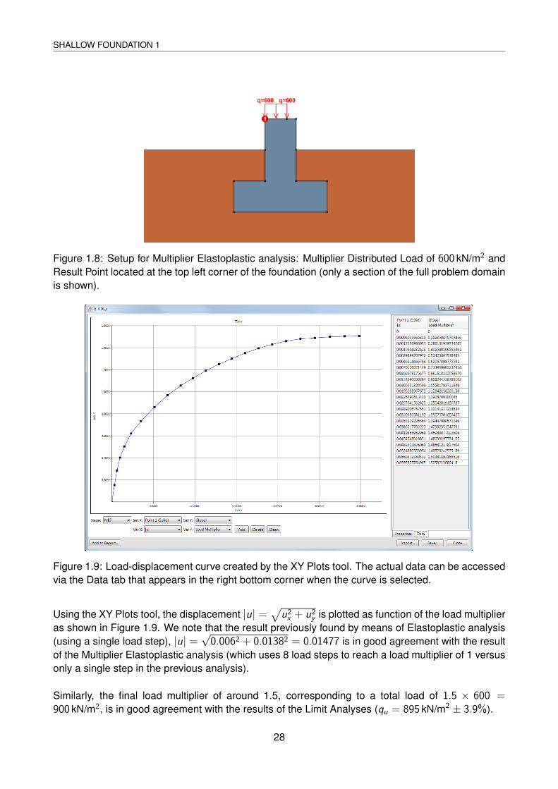
Figure 1.8: Setup for Multiplier Elastoplastic analysis: Multiplier Distributed Load of 600 kN/m2 andResult Point located at the top left corner of the foundation (only a section of the full problem domainis shown).

Figure 1.9: Load-displacement curve created by the XY Plots tool. The actual data can be accessedvia the Data tab that appears in the right bottom corner when the curve is selected.

Using the XY Plots tool, the displacement |u| =√u2x + u2

y is plotted as function of the load multiplieras shown in Figure 1.9. We note that the result previously found by means of Elastoplastic analysis(using a single load step), |u| =

√0.0062 + 0.01382 = 0.01477 is in good agreement with the result

of the Multiplier Elastoplastic analysis (which uses 8 load steps to reach a load multiplier of 1 versusonly a single step in the previous analysis).

Similarly, the final load multiplier of around 1.5, corresponding to a total load of 1.5 × 600 =900 kN/m2, is in good agreement with the results of the Limit Analyses (qu = 895 kN/m2 ± 3.9%).

28

SHALLOW FOUNDATION 1

1.4 Variation of undrained shear strength with depth

The use of a constant undrained shear strength is often a rather crude approximation to reality whereone will usually observe an increase of shear strength with depth. In OptumG2, linear variations ofall parameters can be specified via the righthand side icon that appears when any parameter field isselected (see Figure 1.10).

In the following, a shear strength varying from su = 15 kPa at the top surface (at level of y = 16m)and increasing by 5 kPa/m with depth is used. Such a variation is can be defined using the MaterialParameter dialog shown in Figure (1.10).

y = 16 msu = 15 kPa

5 kPa

1 m

Click to open

Figure 1.10: Specification of linear distribution of su.

Running upper and lower bound limit analysis for this problem gives:

qu = 833.5± 3.5% kN/m2 (1.7)

as compared to the value of qu = 895.0 kN/m2 for a constant su = 30 kPa.

Finally, as a check that the correct distribution of su has been specified, the distribution of all materialparameters can be visualized under Results (see Figure 1.11).

29

SHALLOW FOUNDATION 1

Figure 1.11: Variation of su.

30