1

Segmentation of Medical Images

László Nyúl

Department of Image Processing and Computer GraphicsUniversity of Szeged

nyul@inf.u-szeged.hu

2

X-ray radiography

3

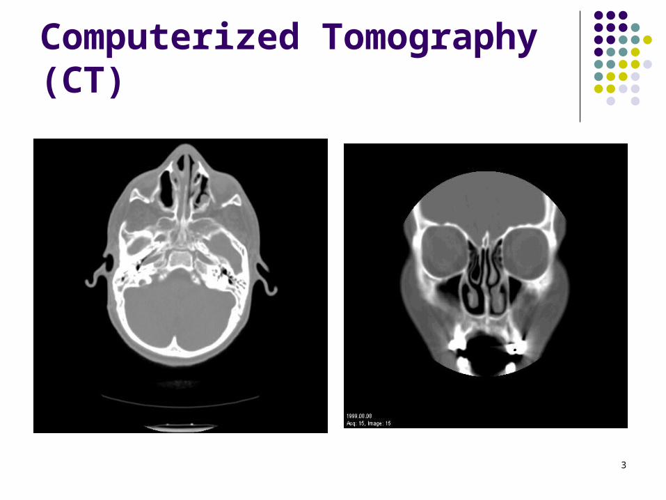
Computerized Tomography (CT)

4

Magnetic Resonance Imaging (MRI)

5

Single Photon Emission CT (SPECT)Positron Emission Tomography (PET)

6

Ultrasound Imaging

7

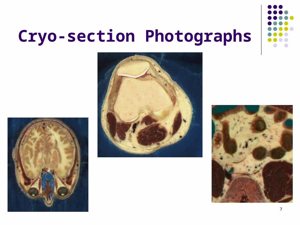
Cryo-section Photographs

8

Thermographic Images

9

Range Images

Reflection image Range image

10

Purpose of 3D Imaging

IN: multiple multimodality images (CT, MR, PET, SPECT, US, …)

OUT: information about an object/object system (qualitative, quantitative)

11

Sources of Images

2D: digital radiographs, tomographic slices 3D: a time sequence of 2D images of a dynamic

object, a stack of slice images of a static object 4D: a time sequence of 3D images of a dynamic

object 5D: a time sequence of 3D images of a dynamic

object for a range of imaging parameters (e.g., MR spectroscopic images of heart)

12

Operations

Preprocessing: for defining the object information Visualization: for viewing object information Manipulation: for altering object information Analysis: for quantifying object information

The operations are independent

13

Preprocessing Operations

Volume of interest (VOI)converts a given scene to another scene of smaller scene domain (ROI) and/or intensity range (IOI)

Filteringconverts a given scene to another scene by suppressing unwanted information and/or enhancing wanted information

14

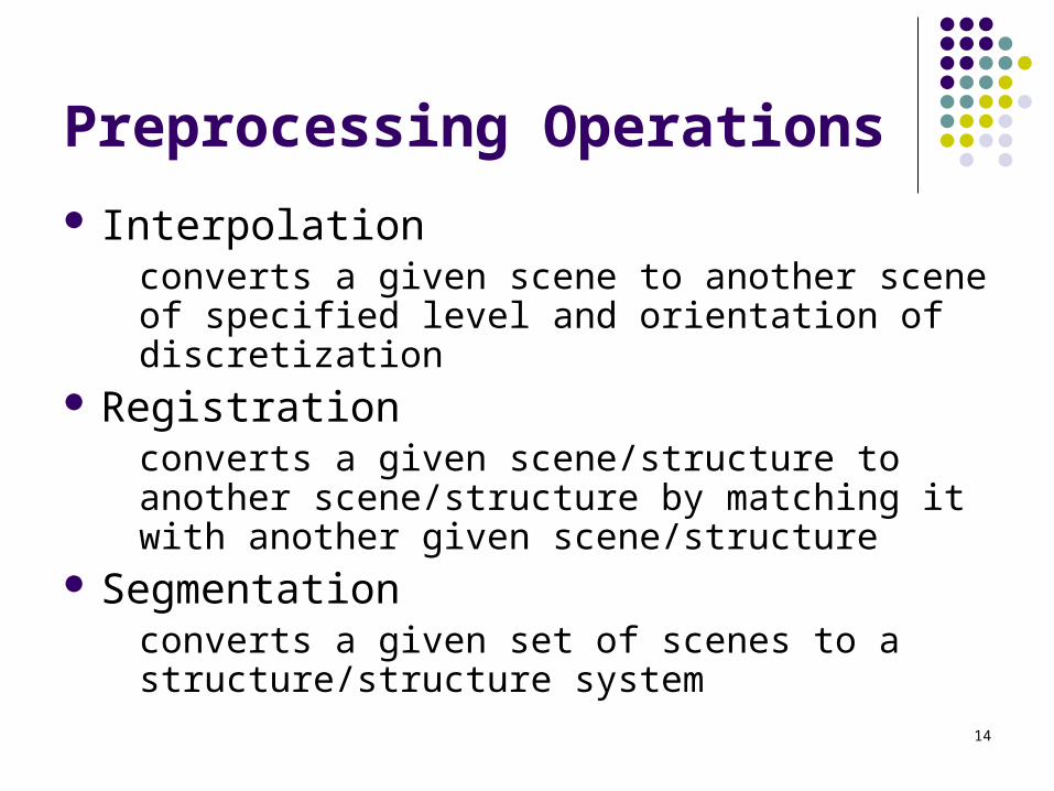
Preprocessing Operations

Interpolationconverts a given scene to another scene of specified level and orientation of discretization

Registrationconverts a given scene/structure to another scene/structure by matching it with another given scene/structure

Segmentationconverts a given set of scenes to a structure/structure system

15

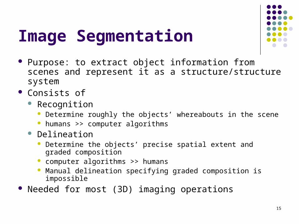
Image Segmentation

Purpose: to extract object information from scenes and represent it as a structure/structure system

Consists of Recognition

Determine roughly the objects’ whereabouts in the scene humans >> computer algorithms

Delineation Determine the objects’ precise spatial extent and graded

composition computer algorithms >> humans Manual delineation specifying graded composition is impossible

Needed for most (3D) imaging operations

16

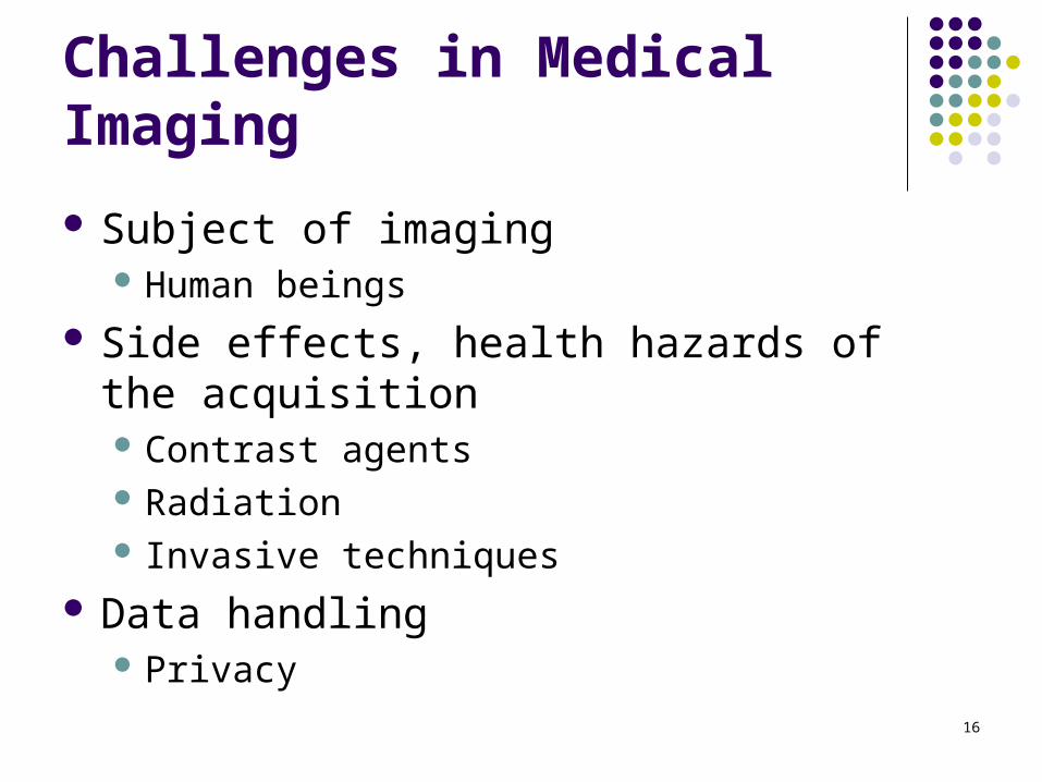
Challenges in Medical Imaging

Subject of imaging Human beings

Side effects, health hazards of the acquisition Contrast agents Radiation Invasive techniques

Data handling Privacy

17

Challenges in Medical Imaging

Image processing Grey-level appearance of tissues Characteristics of imaging modality Geometry of anatomy

Organs are of different size and shape Normal vs. diseased Objects may change between acquisitions

Automated processing is desirable Evaluation

No ground truth available!

18

Limitations of Acquisition Techniques

Resolution Spatial Temporal Density

Tissue contrast Noise distribution, shading Partial volume averaging Artifacts Implants

19

Noise and Sampling Errors

20

Different Tissue Contrast

21

Artifacts

22

Applications of Image Segmentation in Medicine Visualization, qualitative analysis Quantitative analysis

Neurological studies Radiotherapy planning Diagnosis Research Implant design Image guided surgery Surgical planning and simulations Therapy evaluation and follow up …

23

Brain and the Ventricles

24

Regions to Segment

Target regions for quantification and

measurements radiation treatment needle insertion, biopsy surgical resection

Regions to avoid by radiation needle drill surgical knife

25

Computer Aided Diagnosis (CAD)

The computer can store, process, compare, and present (visualize) data

The computer may even make suggestions

The physician has to make the final judgment!

26

Image Segmentation Consists of

Recognition humans >> computer algorithms

Delineation computer algorithms >> humans Manual delineation specifying graded composition is impossible

Aim: exploit the synergy between the two (humans and computer algorithms) to develop practical methods with high PRECISION: reliability/repeatability ACCURACY: agreement with truth EFFICIENCY: practical viability

27

Approaches to Recognition

Automatic Knowledge- and atlas-based artificial intelligence

techniques used to represent object knowledge Preliminary delineation needed to form object

hypotheses Map geometric information from scene to atlas

28

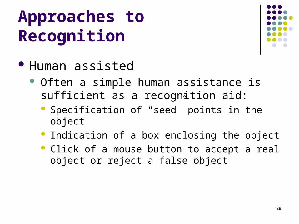
Approaches to Recognition

Human assisted Often a simple human assistance is sufficient as a

recognition aid: Specification of “seed” points in the object Indication of a box enclosing the object Click of a mouse button to accept a real object or

reject a false object

29

Approaches to Delineation

Boundary-based Work with boundaries (contours, surfaces) Output boundary description of objects

Region-based Work with regions (pixels, voxels and patches) Output regions occupied by objects

Hybrid Combine boundary-based and region-based methods

30

Approaches to Delineation

Hard (crisp) Each voxel in the output has a label of belonging either to

object or background

Fuzzy Each voxel in the output has a membership value in both

object and background

31

Boundary-based Segmentation Methods

Align model boundary with object boundary using image features (edges)

Requires initialization near solution to avoid becoming stuck in local minima

Pixel information inside the object is not considered

32

33

Pre-processing (creating boundaries)

Feature detection Points Lines Edges Corners Junctions

Contour following Edge linking Canny edge-detector

34

Iso-surfacing

Produce a surface that separates regions of intensity > threshold from those < threshold

Digital surfaces Voxels Voxel faces Polygonal elements

0 20 30 10 15

20 50 80 20 10

30 70 40 10 20

16 15 20 60 15

10 15 20 30 20

35

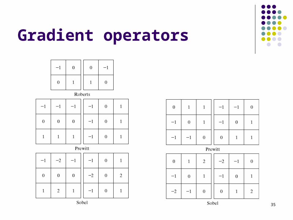
Gradient operators

36

Creating Edges From Image Gradient

37

Degree of “edginess”

38

Hough Transform

Locate curves described by a few parameters Edge points are transformed into the parameter

space and a cumulative map is created Local maximum corresponds to the parameters of a

curve along which several points lie

Straight lines Circles

39

Parameterization of a Line

40

Detecting Lines via Hough Transform

41

Detecting Lines via Hough Transform

42

Detecting Circles via Hough Transform

43

Live Wire Segmentation of the Knee and the Ankle

Live wire Live lane Live wire 3D

44

Deformable Boundaries Active/dynamic contour, snake Active surface Active shape model (ASM) Active appearance model (AAM)

Aim: minimize an energy functional with internal and external energy content

Challenges Tuning the effects of the energy components Handling topology changes during evolution

45

Active Contour

shrink wrap balloon

46

Gradient Vector Field

47

Active Contour with GVF

48

Deformable Surfaces in 3D

Transition from 2D to 3D is not trivial!

2D contour as polygon (vertices, edges) 3D surface as polyhedron (vertices, edges, faces)

Self-crossing Topology changes

Topology adaptive snakes (T-snakes)

49

Affine cell image decomposition (ACID)

50

Active Surface Segmentations of the Liver and the Right Kidney

51

Level-set and Fast Marching Methods

Contour/surface is represented as the zero level set of some evolving implicit function

52

Evolving Level Set Functions

53

Segmenting Vessels and Gray Matter using Level-sets

54

Region-based Segmentation Methods

Image pixels are assigned to object or background based on homogeneity statistics

Advantage is that image information inside the object is considered

Disadvantage is lack of provision for including shape of object in decision making process

55

Thresholding

General form: T = T{ x, A(x), f(x) }

Global: T = T{ f(x) } Local: T = T{ A(x), f(x) } Adaptive / dynamic: T = T{ x, A(x), f(x) }

Single threshold Band thresholding Hysteresis thresholding

Dozens of strategies for determining thresholds

56

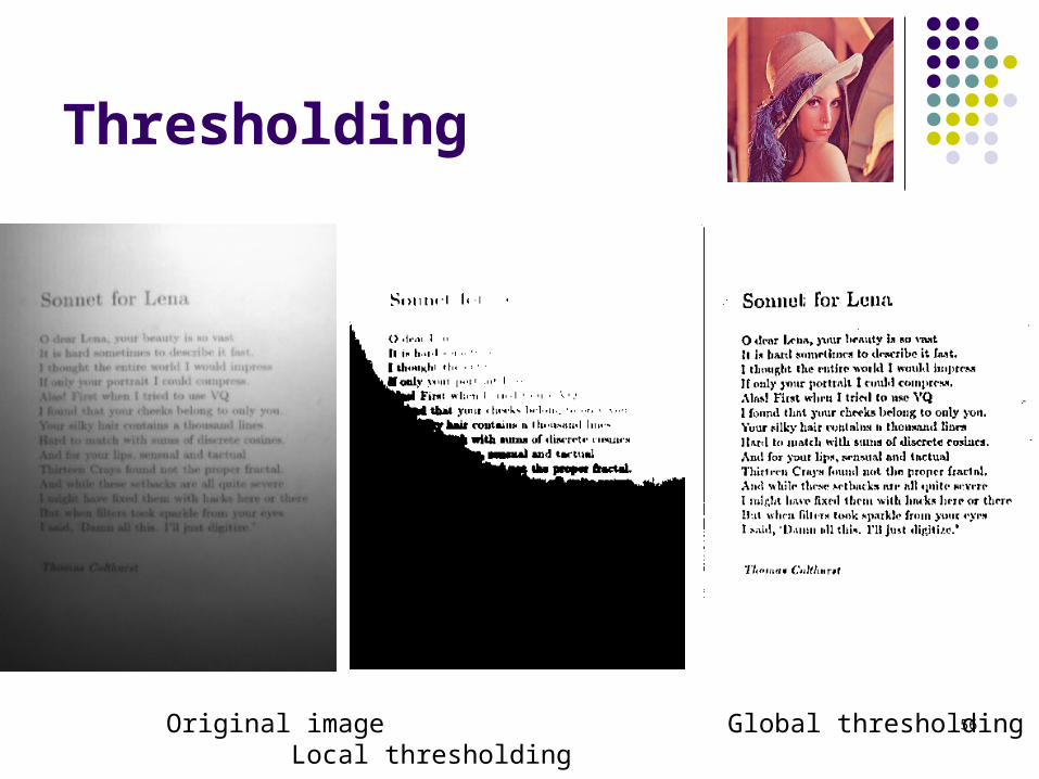
Thresholding

Original image Global thresholding Local thresholding

57

Hounsfield Unit Ranges for CT

58

Fuzzy Image Processing

Why Use Fuzzy Image Processing?

59

Membership functions

60

„young person”

61

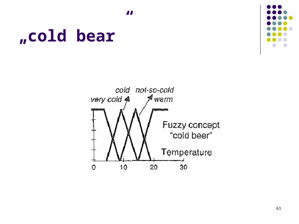
„cold bear”

62

Typical shapes of membership functions

63

Set and its complement

64

General Structure of Fuzzy Image Processing

65

Representing “dark gray-levels” with sets

66

Histogram Fuzzification with Three Membership Functions

67

Fuzzy thresholding

68

Example of fuzzy thresholding

69

Thresholding Using Fuzziness

70

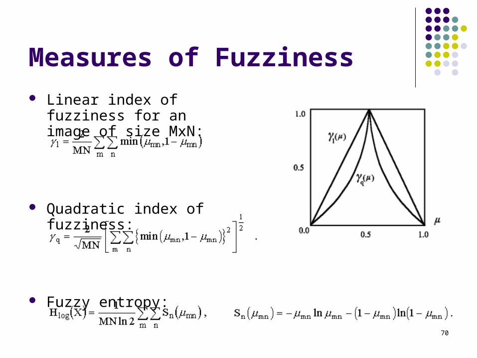
Measures of Fuzziness Linear index of fuzziness for

an image of size MxN:

Quadratic index of fuzziness:

Fuzzy entropy:

71

Clustering Techniques

72

Clustering using two features

73

k-nearest neighbors (kNN) Training: identify two sets of voxels XO in object region and XNO in

background

For each voxel v in input scenes, find its location P in feature space

Find k voxels closest to P from sets XO and XNO

If a majority of those are from XO, v belongs to object, otherwise to background

Fuzzy kNN is possible if m out of k nearest neighbors of voxel v belongs to object, than

we can assign (v)=m/k as the membership of v in the object

74

75

76

Region Growing

1. Specify a (set of) seed voxel(s) in the object and put them in a queue Q. Specify criteria C for inclusion of voxels (such as thresholds on voxel intensity and/or mean intensity and/or variance of growing region)

2. If Q is empty, stop, else take a voxel v from Q and output v

3. Find those neighbors X of v in scene which were not previously visited and satisfy C

4. Put X in Q and go to Step 2.

77

Watershed Algorithm

78

Using Markers to Overcome Over-segmentation

79

Markov Random Fields (MRF)

MRF can be used to model nonlinear interaction between features spatial and temporal information

Cliques Statistical processes

80

Artificial Neural Networks (ANN)

81

Object Characteristics in Images

Graded compositionheterogeneity of intensity in the object region due to heterogeneity of object material, blurring, noise, and background variation caused by the imaging device

Hanging-togetherness (Gestalt)natural grouping of voxels constituting an object a human viewer readily sees in a display of the scene in spite of intensity heterogeneity

Graded composition and hanging-togetherness are fuzzy properties

82

Fuzzy Sets and Relations

Fuzzy subset:

Membership function:

Fuzzy relation:

Fuzzy union and intersection operations(e.g., max and min)

Similitude relation: reflexive, symmetric, transitive

Xxxx |, AA

1,0: XA

XXyxyxyx ,|,,,

1,0: XX

83

Fuzzy Digital Space

Fuzzy spel adjacency: how close two spels are spatially. Example:

Fuzzy digital space:

Scene (over a fuzzy digital scene):

otherwise,0

distance small a if,1

,dc

dcdc

fC,C

,nZ

84

Fuzzy Connectedness

Fuzzy spel affinity:how close two spels are spatially and intensity-based-property-wise (local hanging-togetherness)

Path (between two spels) Fuzzy -net Fuzzy -connectedness (K)

dcdfcfdchdc ,,,,,,

c

d

85

Fuzzy Connected Objects

Binary relation

Fuzzy -component of strength x Fuzzy x object containing o

Very important property: robustness

otherwise,0

, if,1,

dcdcK

86

Fuzzy Connectedness Variants

Multiple seeds per object

Scale-based fuzzy affinity

Relative fuzzy connectedness

Iterative relative fuzzy connectedness

Vectorial … fuzzy connectedness

87

Scale-based Fuzzy Affinity

spatial adjacency homogeneity object feature object scale

global hanging-togetherness

88

Scale As Used in Fuzzy Connectedness “Scale” is the size of local structures under a pre-specified region-

homogeneity criterion. In an image C at any voxel c, scale is defined as the radius r(c) of

the largest ball centered at c which lies entirely within the same object region.

The scale value can be simply and effectively estimated without explicit object segmentation.

89

Applications with Fuzzy Connectedness Segmentation MR

Brain tissue segmentation Brain tumor quantification Image analysis in multiple sclerosis and Alzheimer’s disease

MRA Vessel segmentation, artery-vein separation

CT bone (skull, shoulder, ankle, knee, pelvis) segmentation Kinematics studies Measuring bone density Stress-and-strain modeling

CT soft tissue (fat, skin, muscle, lungs, airway, colon) segmentation Detecting and quantifying cancer, cyst, polyp Detecting and quantifying stenosis and aneurism

Digitized mammography Detecting microcalcifications

Craniofacial 3D imaging Visualization and surgical planning

Visible Human Data

90

Brain Tissue Segmentation (SPGR)A B C D

F G H

J K L M

91

MS Lesion Quantification (FSE)

A B C D

E F G H

92

MTR Analysis

93

Brain Tumor Quantification

A B

C D

94

MRA Vessel SegmentationA B C

FD E

95

HybridSegmentation Methods

Combine boundary-based and region-based methods

Each well understood Utilize strengths of both, reduce exposure to

weakness of either

Advantage More reliable When the region-based method is trapped in a local

minimum, the boundary-based method can drive it out

96

Fuzzy connectedness with Voronoi diagram

Use fuzzy connectedness to generate statistics for homogeneity operator in a color space (e.g., RGB, HCV)

Run Voronoi Diagram-based algorithm in multiple color channels

Identify connected components Use deformable model to determine final (3D)

boundary

9797

Slides with hybrid segmentation Slides with hybrid segmentation examples borrowed from lecture notes of examples borrowed from lecture notes of Celina Imielinska (Columbia University)Celina Imielinska (Columbia University)

9898

Examples:

Understanding Visual Information: Technical, Cognitive and Social Factors_______________________________________________

9999

Method I: Gray Matter

Understanding Visual Information: Technical, Cognitive and Social Factors_______________________________________________

GMGM

WMWM

100100

Fuzzy Connectedness with Voronoi DiagramFuzzy Connectedness with Voronoi Diagram

Fuzzy Connectedness:Fuzzy map

Binary image fromwhich we generatehomogeneity statistics

Voronoi Diagramwith yellow boundaryVoronoi regions

Final boundary:a subgraph of theDelaunay triangulation

101101

Fuzzy Connectedness with Voronoi DiagramFuzzy Connectedness with Voronoi Diagram

FuzzyConnectedness:Fuzzy map

Binary Image (homogeneity statistics)

Voronoi Diagramwith yellowboundary Voronoiregions

Final Boundary:a subgraph of Delaunay Triangulation(click to play movie)

102102

103103

Segmentation of Brain TissueSegmentation of Brain Tissue

104104

Hybrid Segmentation: Visible Human Male: Kidney

Columbia University

Result: FC Result: FC/VD/CCResult: FC/VD Result: FC/VD/CC/DM

Input data Hand Segmentation

105105

Columbia University

Result: FC/VD/CC Result: FC/VD/CC/DM Hand Segmentation

Hybrid Segmentation: Visible Human Male: Kidney

106

Useful Techniques

107

Scale-space and Multi-level/ Multi-scale Techniques

Gaussian Pyramid Reduction of data Gain in processing time Gain in robustness Gain in accuracy

108

Details at Different Scales

109

Details at Different Scales

110

Template Matching with Cross-correlation

111

Other Useful Techniques

Morphological operators Dilation, erosion, opening, closing Cavity filling

Connected component labeling Distance transform

Euclidean City block / Manhattan 3-4-5 chamfer

112

Evaluation of Image Segmentation Methods

113

Measures and Figures of Merit

The method’s effectiveness can be assessed by several sets of measures Precision (reliability) Accuracy (validity) Efficiency (practical viability in terms of the time required)

In fact, effectiveness should be assessed by all measures, since one measure by itself is not always meaningful

114

Precision

Three types of precision is usually measured Intra-operator precision Inter-operator precision Repeat-scan precision

For each test, volume difference and overlap agreement may be measured

For repeat-scan overlap measurement, registration of the two scenes is necessary

115

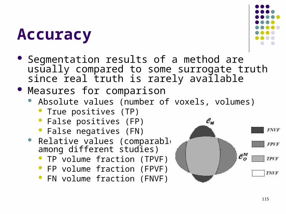
Accuracy Segmentation results of a method are usually

compared to some surrogate truth since real truth is rarely available

Measures for comparison Absolute values (number of voxels, volumes)

True positives (TP) False positives (FP) False negatives (FN)

Relative values (comparable among different studies) TP volume fraction (TPVF) FP volume fraction (FPVF) FN volume fraction (FNVF)

116

Efficiency

Unfortunately, this sort of evaluation is often neglected

Possible measures Running time (wall clock time)

highly dependent on what type of hardware the program is running on

Amount of necessary human interaction number and length of interactive sessions

How convenient it is for the operator the way the human input is required

117

Motto: “There is no silver bullet”

Whatever technique you choose you have to tailor it to the particular application context

This usually means not only setting parameters but also designing new algorithms built from existing ones, combining different pre- and post-processing techniques with robust algorithms, sometimes even combining several segmentation algorithms to achieve the goal, designing workflows, user interfaces, and validation methods