1-s2.0-s1877050910000712-main

Available online at www.sciencedirect.com

Procedia Computer Science 00 (2009) 000–000

Procedia Computer Science

www.elsevier.com/locate/procedia

International Conference on Computational Science, ICCS 2010

Cyclohexane/water dispersion behaviour in a stirred batch vessel experimentally and with CFD simulation

L. Abu-Faraha,*, F. Al-Qaessia, A. Schönbuchera

aUniversität Duisburg-Essen, Institut für Technische Chemie I, Universitätsstr. 7, Essen 45117, Deutschland

Abstract

Cyclohexane/water dispersion behaviour is studied in a stirred batch vessel with rushton turbine impeller (RTI), experimentally and with computational fluid dynamic (CFD) simulation. The axial and radial holdup profiles and distribution of cyclohexane in the whole vessel are measured by using the sampling withdrawal method from different positions in the vessel at different stirrer velocities. The minimum stirrer velocity to get a complete dispersion and a uniform distribution of cyclohexane in water is also determined. The dispersion behaviour of cyclohexane in water is visualized by using a video camera and a red color tracer. Steady 3-dimensional simulations with Eulerian-Eulerian multi-fluid model are used to calculate the dispersion behaviour and the volumetric fractions of cyclohexane in the vessel by using ICEM CFD and Ansys CFX-11. The two equations k-ε turbulent model is included to calculate the velocity flow field. The interphase momentum transfer and the drag forces between the continuous and dispersed phases are calculated by using algebraic slip mixture (ASM) and Ishii-Zuber models. Sliding mesh model is used to model the interaction between the rotating impeller and the vessel walls. The effect of grid size on the calculations is studied. A good agreement between the predicted CFD and the experimental data is obtained.

Keywords: CFD simulation; multiphase liquids; rushton turbime; holdup; ASM; visualization

1. Introduction

Immiscible liquid-liquid dispersions are considered in many industrial applications such as chemical, petroleum, pharmaceutical and biochemical processes such as liquid-liquid extraction, suspension polymerization and chemical reactions, with the objective to increase the contact area between the two phases [1][2]. Dispersions are defined as mixtures of two immiscible fluids with one dispersed as drops in a second fluid which forms a continuous phase [3]. The purposes of this operation are to mix two phases, increase the interfacial area and to enhance the mass transfer between the two phases [1]. When two immiscible liquids are combined in a mixing vessel, it is required to know the minimum stirrer velocity for both complete and uniform dispersion of one liquid in the other [4]. This can be determined when the dispersed phase visually disappears and becomes completely incorporated into the bulk of the liquid [5][6][7]. Bouyatiotis et al. [8] measured the holdup of different organics as a dispersed phase in water as a continuous phase in a stirred continuously operating tank. They found that when the holdup increases, the mean droplet size also increases. In their study when the local volume fraction of the dispersed phase remains constant with the same value at different positions in the vessel, then the complete and uniform dispersion is achieved. The knowledge of the dispersion and distribution of the dispersed phase is essential in determination of rates of mass transfer and for design and scale up of the mixing equipment [9]. Insufficient understanding of these mixing processes causes the continuous loss of a large amount of money.

The interfacial area is affected by different variables such as volume fraction of the dispersed phase, fluid properties of the continuous and dispersed phases and the mechanical mixing conditions like the vessel size, stirrer size and flow velocity [10]. Few studies have been done on the experimental investigation and numerical prediction of immiscible liquid-liquid dispersion in stirred vessel and they focused on the measurements of the drop size distribution [11][12]. Previous CFD investigations focused

* Corresponding author. Tel.: +49-0-201-183-3141; fax: +49-0-201-183-3049. E-mail addresses: [email protected] (L. Abu-Farah), [email protected] (F. Al-Qaessi), [email protected] (A. Schönbucher).

c⃝ 2012 Published by Elsevier Ltd.

Procedia Computer Science 1 (2012) 655–664

www.elsevier.com/locate/procedia

1877-0509 c⃝ 2012 Published by Elsevier Ltd.doi:10.1016/j.procs.2010.04.070

http://www.elsevier.com/locate/procedia

http://dx.doi.org/10.1016/j.procs.2010.04.070

Author name / Procedia Computer Science 00 (2010) 000–000

on the multiphase mixing processes of gas-liquid and solid-liquid systems [13]. CFD simulation of the hydrodynamics in stirred vessels is very difficult because the flow field in the tank is complex and highly unsteady due to the interaction of the rotating impeller with multiphase dispersion [14]. The difficulties in the simulation are the accurate selection of the appropriate model of the interphase interaction and the turbulence flow. The flow field and turbulence in stirred vessels have a significant effect on the volumetric fractions of the dispersed phase, the minimum required stirrer velocity to get a complete and uniform dispersion [15][16]. Turbulence consists of high energy eddies near the impeller, and lower energy eddies are located farther away from the impeller [17]. These complex phenomena can be investigated by using a CFD, because the experimental approaches are insufficient for the insight of the liquid-liquid dispersions. The progress on the simulation of multiphase flow in stirred vessels is much less than that in chemical reactors like bubble and extraction columns, spray towers and fluidization beds [18].

The aim of this study is to understand the physical and interfacial phenomena which involve the dispersion behaviour of cyclohexane in water experimentally and with CFD simulation by using Eulerian multiphase approach. Ansys CFX-11 is used for solving the differential equations. The minimum stirrer velocity for complete and uniform dispersion is determined from the measurements of the axial and radial profiles of cyclohexane volume fraction, and from the visualisation method of the flow field and the distribution of cyclohexane into water by using a video camera and a red tracer. With the CFD simulations, the effects of the interphase momentum transfer model and the grid size on the dispersion behaviour of cyclohexane/water system are predicted. Turbulence effect is included in the CFD simulations. The effect of the radial flow by the RTI on the hold up distribution of cyclohexane is presented. The predicted data are compared with the experimental results.

2. Experimental

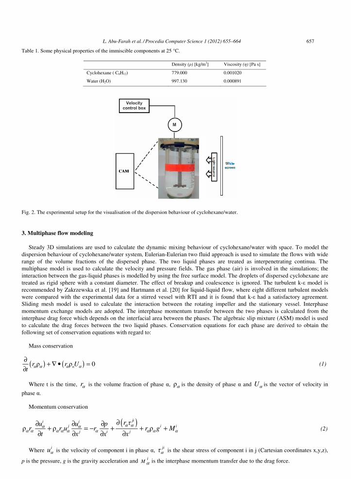
Mixing of cyclohexane/water is carried out in a non-baffled rounded bottom batch vessel, stirred with 6-blades RTI which is connected to the velocity controller through the motor (M), see Fig.1. (a). The dimensions of the vessel and RTI are illustrated in Fig. 1. (b). The surface tension between the dispersed cyclohexane and continuous water phases is 0.05 N/m. Other physical properties of the two phases can be seen in table 1. The sampling withdrawal method is used for measuring the hold up of cyclohexane with the help of the vacuum pump, to collect different samples of the cyclohexane/water dispersions in the radial and axial positions. The experimental setup for measuring the volume fraction of cyclohexane in water is shown in Fig. 1. (a). The stirred vessel is charged with 400 mL (80 vol %) distilled water, 100 mL (20 vol %) of cyclohexane is added slowly to the vessel, forming the top lighter layer which has the lower density. The total height of the liquid phases is 11 cm. A sampling tube made of stainless steel with a diameter of 1.0 mm is fixed in the axial or radial position. The motor is started with the stirring velocity of 350 rpm. After an equilibration period varying between 10 and 15 min is reached, the vacuum pump system is activated. Then the triple valve will be opened to permit the liquid flow from the vessel through the sampling tube into the reservoir to collect a volume of 10 mL. After that this valve is closed and will be opened in a direction to permit the liquid flow from the vessel into the collector to collect a sample of about 10 mL. This sample is discharged into a graduated cylinder and is allowed to separate into two phases to determine the volume fraction of the dispersed phase in the sample. All the liquids will be returned to the vessel to ensure the sampling system delivers the representative samples. The same procedure is repeated at different radial and axial sampling points and at different stirrer velocities to cover the range from the incipient dispersion to the nearly uniform dispersion. The minimum stirrer velocity for complete and uniform dispersion, the dispersion behaviour and flow field of cyclohexane into water are visualized by using a video camera (CAM) and a red tracer, see Fig. 2.

(a) (b)

Fig. 1. (a) Schematic experimental setup for volume fraction measurements; (b) The dimensions of the vessel and RTI with diameter D = 3.3 cm, bottom clearance B = 3.2 cm, shaft diameter S = 1 cm, vessel height H = 16 cm, total liquid height Hl = 11 cm, RTI diameter to the vessel diameter D/dv = 0.41, disk diameter to the RTI diameter dd/D = 0.75, blade width b = 0.25D = 0.825 cm and blade thickness w = 0.2D = 0.66 cm.

656 L. Abu-Farah et al. / Procedia Computer Science 1 (2012) 655–664


Table 1. Some physical properties of the immiscible components at 25 °C.

Density (ρ) [kg/m3] Viscosity (η) [Pa s]

Cyclohexane ( C6H12) 779.000 0.001020

Water (H2O) 997.130 0.000891

Fig. 2. The experimental setup for the visualisation of the dispersion behaviour of cyclohexane/water.

3. Multiphase flow modeling

Steady 3D simulations are used to calculate the dynamic mixing behaviour of cyclohexane/water with space. To model the dispersion behaviour of cyclohexane/water system, Eulerian-Eulerian two fluid approach is used to simulate the flows with wide range of the volume fractions of the dispersed phase. The two liquid phases are treated as interpenetrating continua. The multiphase model is used to calculate the velocity and pressure fields. The gas phase (air) is involved in the simulations; the interaction between the gas-liquid phases is modelled by using the free surface model. The droplets of dispersed cyclohexane are treated as rigid sphere with a constant diameter. The effect of breakup and coalescence is ignored. The turbulent k-ε model is recommended by Zakrzewska et al. [19] and Hartmann et al. [20] for liquid-liquid flow, where eight different turbulent models were compared with the experimental data for a stirred vessel with RTI and it is found that k-ε had a satisfactory agreement. Sliding mesh model is used to calculate the interaction between the rotating impeller and the stationary vessel. Interphase momentum exchange models are adopted. The interphase momentum transfer between the two phases is calculated from the interphase drag force which depends on the interfacial area between the phases. The algebraic slip mixture (ASM) model is used to calculate the drag forces between the two liquid phases. Conservation equations for each phase are derived to obtain the following set of conservation equations with regard to:

Mass conservation

( ) ( )ρ ρ 0αr r Ut α α α α

∂+ ∇ • =

∂ (1)

Where t is the time, rα is the volume fraction of phase α, ρα is the density of phase α and Uα is the vector of velocity in

phase α.

Momentum conservation

( )ρ ρ ρ

jii ij i i

j i j

r τu u pr r u r r g M

t x x xα αα α

α α α α α α α α α

∂∂ ∂ ∂+ = − + + +

∂ ∂ ∂ ∂ (2)

Where iuα is the velocity of component i in phase α, jiτα is the shear stress of component i in j (Cartesian coordinates x,y,z),

p is the pressure, g is the gravity acceleration and iM α is the interphase momentum transfer due to the drag force.

L. Abu-Farah et al. / Procedia Computer Science 1 (2012) 655–664 657


P

3

4 di ii

D S S

rM C u uα

αα α

ρ= − (3)

Where CD is the drag coefficient, dp is the mean droplet diameter and iSu α is the slip velocity of component i in phase α.

Turbulence model The transport equations of k and ε for the standard k-ε model can be written as

( )( ) tρρ ρk

k

kUk k P

t σ

⎡ ⎤⎛ ⎞∂ μ+ ∇ • = ∇ • μ + ∇ + − ε⎢ ⎥⎜ ⎟

∂ ⎝ ⎠⎣ ⎦ (4)

( )( ) ( )tρρ ρg1 k g2U C P C

t kσ ε

⎡ ⎤⎛ ⎞∂ ε μ ε+ ∇ • ε = ∇ • μ + ∇ε + − ε⎢ ⎥⎜ ⎟

∂ ⎝ ⎠⎣ ⎦ (5)

Where ε is the energy dissipation, k is the kinetic energy, g1C , g2C , kσ and

εσ are constants, kP is the turbulence production due

to viscous and buoyancy forces and tμ is the turbulence viscosity.

The above equations are discretized by using the finite volume method with high resolution advection scheme, which allows the calculations of the phase velocities, volume fractions and slip velocity of the dispersed phase. Steady simulations with 10000 iterations are set to get sufficient accurate and precise results. The solution is considered converged when the residuals in the solved equations become smaller than prescribed tolerance of 0.0001.

3.1 Geometry and grid generation

ICEM CFD 5.1 is used to create the 3D full geometry rounded bottom stirred vessel and RTI with the same dimensions as those used in the experiment in Fig. 1. (a). Unstructured tetrahedral cells are used for the generation of such complex geometry. The meshing limitations are to optimize the CPU time of the simulation with precise calculations. Two separate assemblies are constructed, one is for the rotating part (RTI) and the second is for the stationary part (the rest parts of the vessel i.e. cylindrical walls, bottom, wall top and the shaft). New interfaces are created between the stationary and rotating regions as shown in Fig. 3.The unstructured tetrahedral cells with cell size of 0.001 m are generated for both assemblies; the total numbers of the unstructured tetrahedral cells for the stirred vessel with RTI are 1330115.

Fig. 3. The grid for the full geometry in the sliding mesh method. The stationary vessel (left) and rotating RTI (right) regions.

3.2 Initial and boundary conditions

Cyclohexane (the lighter phase) is set on the top part of the vessel with 20 vol % of the total liquid volume and the water (the heavier phase) is placed in the bottom part of the vessel. The initial conditions for the pressure field and volume fraction at t = 0



are defined by using the command expression language (CEL) and the time step functions. The boundary conditions at the bottom and vessel walls are those derived assuming no-slip condition and counter rotating walls (stationary walls). No-slip means that the velocity of the fluid at the wall boundary is set to zero regarding to Dirichlet condition. No-slip boundary conditions are used at the RTI impeller and the shaft. An opening boundary condition is employed for the wall top of the domain to allow only the air to flow through but not the liquid phase. Rotor stator method is used to calculate the flow velocity between the RTI and the vessel.

4. Results and discussion

4.1 Dispersion behaviour of cyclohexane/water system

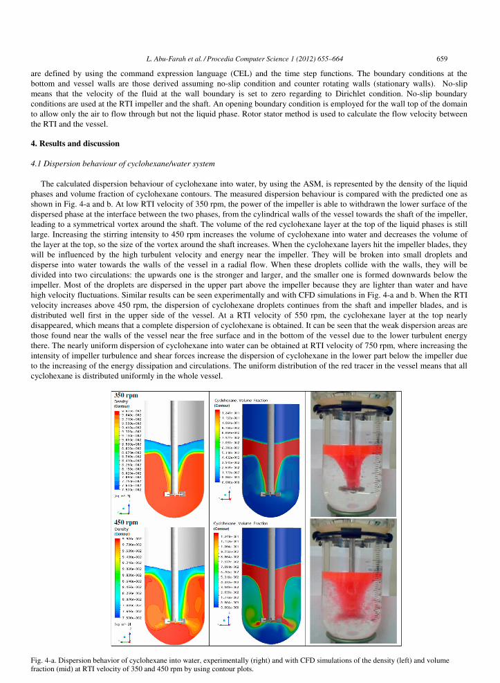
The calculated dispersion behaviour of cyclohexane into water, by using the ASM, is represented by the density of the liquid phases and volume fraction of cyclohexane contours. The measured dispersion behaviour is compared with the predicted one as shown in Fig. 4-a and b. At low RTI velocity of 350 rpm, the power of the impeller is able to withdrawn the lower surface of the dispersed phase at the interface between the two phases, from the cylindrical walls of the vessel towards the shaft of the impeller, leading to a symmetrical vortex around the shaft. The volume of the red cyclohexane layer at the top of the liquid phases is still large. Increasing the stirring intensity to 450 rpm increases the volume of cyclohexane into water and decreases the volume of the layer at the top, so the size of the vortex around the shaft increases. When the cyclohexane layers hit the impeller blades, they will be influenced by the high turbulent velocity and energy near the impeller. They will be broken into small droplets and disperse into water towards the walls of the vessel in a radial flow. When these droplets collide with the walls, they will be divided into two circulations: the upwards one is the stronger and larger, and the smaller one is formed downwards below the impeller. Most of the droplets are dispersed in the upper part above the impeller because they are lighter than water and have high velocity fluctuations. Similar results can be seen experimentally and with CFD simulations in Fig. 4-a and b. When the RTI velocity increases above 450 rpm, the dispersion of cyclohexane droplets continues from the shaft and impeller blades, and is distributed well first in the upper side of the vessel. At a RTI velocity of 550 rpm, the cyclohexane layer at the top nearly disappeared, which means that a complete dispersion of cyclohexane is obtained. It can be seen that the weak dispersion areas are those found near the walls of the vessel near the free surface and in the bottom of the vessel due to the lower turbulent energy there. The nearly uniform dispersion of cyclohexane into water can be obtained at RTI velocity of 750 rpm, where increasing the intensity of impeller turbulence and shear forces increase the dispersion of cyclohexane in the lower part below the impeller due to the increasing of the energy dissipation and circulations. The uniform distribution of the red tracer in the vessel means that all cyclohexane is distributed uniformly in the whole vessel.

Fig. 4-a. Dispersion behavior of cyclohexane into water, experimentally (right) and with CFD simulations of the density (left) and volume fraction (mid) at RTI velocity of 350 and 450 rpm by using contour plots.



Fig. 4-b. Dispersion behavior of cyclohexane into water, experimentally (right) and with CFD simulations of the density (left) and volume fraction (mid) at RTI velocity of 550, 650 and 750 rpm by using contour plots.

4.1.1 Effect of different momentum transfer models and different grid sizes

The predicted dispersion behaviour of cyclohexane into water from ASM and Ishii-Zuber models are compared with that visualised at RTI velocity of 550 rpm as can be seen in Fig. 5-a, b and c for grid size of 0.001 m. The dispersion behaviour and the flow field of cyclohexane into water by using ASM coincide well with that obtained from the visualisation. With the ASM, the dispersion of cyclohexane into water is higher, where the cyclohexane layer at the top of the liquid phase is completely drawn into water, to reach the lowest point in the stirrer and spread towards the walls of the vessel in the radial direction. ASM alongwith the Eulerian multiphase model assume mutual interpenetration of the phases. The calculated drag force between the two phases from the ASM is high, whereas the relative velocity between the cyclohexane droplets and water are nearly low, and it goes to zero when a uniform dispersion is obtained at a minimum RTI velocity of 750 rpm. The calculated drag force by Ishii-Zuber model is influenced by the gravitational and surface tension forces that keep on the interface between the phases without breakage. Reducing the cell size from 0.004 m to 0.001 m is studied in the case of the simulation with Ishii-Zuber model. Fine mesh is very important in the case of RTI because there are two separate domains: the rotating small 6-blades RTI and the vessel. If the mesh is not enough fine, there will be a gap between the small cells at the RTI and the large cells at the vessel, thus the both grids will not coincide with each other on the surfaces at the interface, so there will be missed data and inconsistency of the calculated variables in the two domains, resulting in a high numerical discretization error. The cell size of 0.004 m gives inconsistent volume fraction distribution of cyclohexane in comparison with that given from the cell size of 0.001m, see Fig. 5-c and d.



Fig. 5. Dispersion behaviour of cyclohexane in water: (a) Experimentally and with CFD simulations at RTI velocity of 550 rpm by using (b) ASM model with cell size of 0.001 m; (c) Ishii-Zuber model with cell size of 0.001 m and (d) Ishii-Zuber model with cell size of 0.004 m.

4.2 Effect of the RTI velocity on the volumetric fractions of cyclohexane

The mixing efficiency of the two liquids is evaluated on the basis of the local volume fraction distribution for the dispersed phase at different stirrer velocities. The measured and calculated local volume fractions of cyclohexane are plotted as a function of the axial, z, from the impeller level to the top near the free surface and radial, r, distances from the shaft to the cylindrical wall of the vessel as can be seen in Fig. 6. The cyclohexane is highly concentrated near the shaft at r = 0.5 cm in Fig. 6-a, and it requires a velocity greater than 750 rpm to shift the whole cyclohexane towards the walls of the vessel, and enhance the dispersion efficiency. The minimum uniform cyclohexane volume fraction of about 0.45 is obtained at RTI velocity of 750 rpm. The uniform distribution of cyclohexane volume fractions in the axial distances between z = 4 and 9 cm can be obtained at a minimum RTI velocity of about 650 rpm, where nearly similar values of the volume fractions are obtained, and a small air vortex around the shaft is formed above z = 8 cm. When the RTI rotates at a velocity of 350 rpm, it is pulled down into water towards the impeller around the shaft, so the concentration of cyclohexane is high at the top, about 3 cm below the free surface between z = 8 to 11 cm and low near the impeller level. This result coincides with the predicted distribution and visualised dispersion behaviour of cyclohexane in section 4.1 in Fig. 4-a and b. The thickness of the cyclohexane layer decreases as the RTI velocity increases, it disappears at a velocity ≥ 550 rpm, see Fig. 6-a. When the impeller velocity increases, the local values of the cyclohexane volume fractions become more uniform and reach nearly the initial value of 0.2 at t = 0 throughout the vessel, a way from the shaft at r ≥ 1.5 cm, see Fig. 6-b to f. The trend of the axial and radial cyclohexane volume fraction profiles is nearly similar at r ≥ 1.5 cm and 4 cm ≤ z ≤ 8 cm, because the cyclohexane is uniformly distributed in this region that is affected by the circulation above the RTI, which enhance the redispersion of cyclohexane droplets. The volume fractions of cyclohexane increase at the axial distances from z = 4 to 8 cm and decreases from z = 10 to 8 cm. At high RTI velocities, the intensity of the radial flow increases as well as the turbulent velocity and the dissipation energy which vary with the location. The highest turbulence intensity and kinetic energy is found near the impeller blades which are responsible on the degree of collisions between the cyclohexane droplets with the vessel walls and the bulk liquid, to increase the dispersion efficiency through the periodic flow and existence of the two vortices above and below the impeller. Cyclohexane is pulled down into the bulk from a radial distance from the shaft that equivalent to the impeller radius (at the highest velocity axis, z) at r = 2 cm and z = 9 cm at the interface between the two phases, see Fig. 6-c. The radial profile of cyclohexane volume fraction at z = 10 cm in Fig. 6-g shows that the unmixed cyclohexane exists at all radial positions at RTI velocity of 350 rpm, and up to r = 2 cm at RTI velocity of 450 rpm. The cyclohexane near the walls at r > 2.5 cm is firstly dispersed into water towards the shaft. Air vortex near the shaft is formed at a minimum RTI velocity of 650 rpm between the shaft and r = 1.5 cm. The initial total liquid height is about 11 cm. The depth of the air vortex is about 1 cm. The uniform cyclohexane volume fraction of about 0.2 at z = 10 cm is obtained at RTI velocity of 650 rpm, see Fig. 6-g.

4.2.1 Complete dispersion velocity

When the velocity of RTI increases the holdup of cyclohexane into water increases in the axial and radial directions as described in section 4.2. The minimum velocity to get a complete dispersion is 550 rpm at r = 0.5 cm, 450 rpm at r = 1.5 and 2 cm and 400 rpm at r = 2.5, 3 and 4 cm, see Fig. 6. The minimum velocity to get a uniform dispersion is 750 rpm at r = 0.5 cm near the shaft, 650 rpm at r = 1.5 and 2 cm, 550 rpm at r = 2.5 and 3 cm and 650 rpm at r = 4 cm near the wall. The uniform cyclohexane volume fraction near the shaft is about 0.45, and about 0.2 in the vicinity of the vessel. For that the minimum velocity to get a complete dispersion is 550 rpm and to get a nearly uniform dispersion is 750 rpm in the whole radial positions in the vessel, thus the RTI velocity should be greater than 750 rpm to get a homogeneous distribution in the whole vessel.



(g)

z = 10 cm

0.0

0.2

0.4

0.6

0.8

1.0

1.2

0.5 1 1.5 2 2.5 3 3.5 4 4.5 5 5.5 6

r [cm]

Cyc

loh

exan

e vo

lum

e fr

acti

on 350 rpm, Exp

350 rpm, CFD

450 rpm, Exp

450 rpm, CFD

550 rpm, Exp

550 rpm, CFD

650 rpm, Exp

650 rpm, CFD

750 rpm, Exp

750 rpm, CFD

Fig. 6. Measured and CFD predicted axial (a-f) and radial (g) cyclohexane volume fraction profiles at different RTI velocities.

(a)

r = 0.5 cm

0.0

0.1

0.2

0.3

0.4

0.5

0.6

0.7

0.8

0.9

1.0

1 2 3 4 5 6 7 8 9 10z [cm]

Cyc

loh

exan

e vo

lum

e fr

acti

on

350 rpm, Exp

350 rpm, CFD

450 rpm, Exp

450 rpm, CFD

550 rpm, Exp

550 rpm, CFD

650 rpm, Exp

650 rpm, CFD

750 rpm, Exp

750 rpm, CFD

(b)

r = 1.5 cm

0.0

0.1

0.2

0.3

0.4

0.5

0.6

0.7

0.8

0.9

1.0

4 5 6 7 8 9 10z [cm]

Cyc

loh

exan

e vo

lum

e fr

acti

on

350 rpm, Exp 350 rpm, CFD





(c)

r = 2 cm

0.0

0.1

0.2

0.3

0.4

0.5

0.6

0.7

0.8

0.9

1.0

4 5 6 7 8 9 10z [cm]

Cyc

loh

exan

e vo

lum

e fr

acti

on






(d)

r = 2.5 cm

0.0

0.1

0.2

0.3

0.4

0.5

0.6

0.7

0.8

0.9

1.0

4 5 6 7 8 9 10z [cm]

Cyc

loh

exan

e vo

lum

e fr

acti

on






(e)

r = 3 cm

0.0

0.1

0.2

0.3

0.4

0.5

0.6

0.7

0.8

0.9

1.0

4 5 6 7 8 9 10z [cm]

Cyc

loh

exan

e vo

lum

e fr

acti

on






(f)

r = 3.5 cm

0.0

0.1

0.2

0.3

0.4

0.5

0.6

0.7

0.8

0.9

1.0

4 5 6 7 8 9 10z [cm]

Cyc

loh

exan

e vo

lum

e fr

acti

on








4.2.2 Effect of the momentum transfer model and grid cell size

The ASM gives a very good agreement between the calculated and measured cyclohexane volume fractions rather than the Ishii-Zuber model at RTI velocity of 550 rpm as shown in Fig. 7-a. The axial profile of cyclohxane volume fraction by using ASM coincides with that obtained from the sampling method for the same reasons described in section 4.1.1. A thin layer of cyclohexane can be found at the top of the liquid phases at z = 10 cm, and the cyclohexane is concentrated around the shaft and blades of the RTI, with few dispersion in the radial direction, this can be seen clearly at r = 2.5 and 3.5 cm in Fig. 7-a. The results of the volumetric fractions distribution of cyclohexane in Fig. 7-a and that visualised in Fig.5-a are in a good agreement. Using a grid with cell size of 0.001 m gives values of cyclohexane volume fractions that follow the axial profile trend of the measured cyclohexane volume fractions at the RTI velocity of 550 rpm and at different distances from the shaft in the radial direction, see Fig. 7-b. It is found that refinement of the mesh in the case of stirred vessel with RTI is important for better matching the both grids of the impeller and the vessel, to get accurate calculations.

(a)

v = 550 rpm

0.0

0.2

0.4

0.6

0.8

1.0

1.2

0 1 2 3 4 5 6 7 8 9 10z [cm]

Cyc

loh

exan

e vo

lum

e fr

acti

on

r = 0.5 cm, Exp

r = 0.5 cm, Ishii

r = 0.5 cm, ASM

r = 1.5 cm, Exp

r = 1.5 cm, Ishii

r = 1.5 cm, ASM

r = 2.5 cm, Exp

r = 2.5 cm, Ishii

r = 2.5 cm, ASM

r = 3.5 cm, Exp

r = 3.5 cm, Ishii

r = 3.5 cm, ASM

(b)

v = 550 rpm

0.0

0.2

0.4

0.6

0.8

1.0

1.2

0 1 2 3 4 5 6 7 8 9 10z [cm]

Cyc

loh

exan

e vo

lum

e fr

acti

on

r = 0.5 cm, Exp

r = 0.5 cm, CS = 0.004 m

r = 0.5 cm, CS = 0.001 m

r = 1.5 cm, Exp

r = 1.5 cm, CS = 0.004 m

r = 1.5 cm, CS = 0.001 m

r = 2.5 cm, Exp

r = 2.5 cm, CS = 0.004 m

r = 2.5 cm, CS = 0.001 m

r = 3.5 cm, Exp

r = 3.5 cm, CS = 0.004 m

r = 3.5 cm, CS = 0.001 m

Fig. 7. Cyclohexane volume fraction profile at different axial and radial positions for RTI velocity of 550 rpm, experimentally and with CFD simulation (a) ASM and Ishii Zuber models for cell size (CS) of 0.001 m; (b) Ishii-Zuber model with cell size of 0.001 and 0.004 m.

5. Conclusions and outlook

The turbulent dispersed phase flow field and holdup in unbaffled batch vessel for a wide range of RTI velocities are predicted with CFD and show a good agreement with the experimental data. It is concluded that the Eulerian-Eulerian model along with the ASM and the k-ε models are able to predict the axial and radial volumetric fractions of cyclohexane. The results of the dispersion behaviour of cyclohexane/water from the visualisation and CFD simulation coincide with the results of the cyclohexane volume fractions profiles in the whole vessel. The predicted density and cyclohexane volume fraction distribution describe well the dispersion of cyclohexane /water system at a wide range of RTI velocity, and show a good agreement with that obtained from the visualisation. The minimum velocity for complete dispersion of cyclohexane into water from the sampling and visualisation methods is about 550 rpm. The uniform dispersion of cyclohexane in the axial distances for a given radial position is obtained at RTI velocity of 650 rpm, whereas in the radial distances for a given axial position is obtained at a minimum velocity of 750 rpm. It is found that the grid size should not exceed 0.001 m for a good prediction. The future work is to design and scale up of liquid-liquid dispersion vessels by means of CFD.

References

1. Feng Wang and Zai-Sha Mao, Ind. Chem. Res. 44 (2002) 5776-5787.

2. Fredrik J.E. Svenss and Anders Rasmuson, Chem. Eng. Technol. 27 (2004) 335-339.

3. F.B. Alban, S. Sajjadi, M. Yianneskis, Trans. IChemE, Part A, Chemical Engineering Research and design 82, A8 (2004) 1054-1060.

4. A.H.P. Skelland and Jal Moon Lee, Ind. Eng. Chem. Process Des. Deu. 17, No. 4 (1978) 473-478.

5. Piero M. Armenante and Yu-Tsang Huang, Ind. Eng. Chem. Res. 31 (1992) 1398-1406.

6. A.H.P. Skelland and R. Seksaria, Ind. Eng. Chem. Process Des. Dev. 17, No. 1 (1978) 56-61.

7. M. Gaggero, E. Arato, P. Costa, 6th Euoropean conference on Mixing, Pavia, Italy, 1988.

8. B.A. Bouuyatiotis and J.D.Thonton, I.chem.E. Symposium series No. 26 (1967) 43-51.

9. Feng Wang, Zai-Sha Mao, Yuefa Wang, Chao Yang, Chemical Engineering Science. 61 (2006) 7535-7550.

10. R.E. Eckert and C.M. McLaughlin, J.H. Rushton, AICHE Journal 31, No.11 (1985) 1811-1820.

11. R.V. Calabrese, T.P.K. Chang, P.T. Dang, AICHE Journal 32, (1986) 657-666.

12. G. Zhou and S.M. Kresta, Chem. Eng. Sci. 53 (1998) 2063-2079.



13. Wang Weijing and Mao Zaisha, Chines J. Chem. Eng., 10 (4) (2002) 385-395.

14. J.G. Van De Vusse, Chem. Eng. Sci. 4 (1955) 178-200.

15. A.C. Johansson and J.C. Godfrey, Recents Progres en Genie des Procedes 11, No. 52 (1997) 255-262.

16. Joachim Ritter and Mathias Kraume, Chem. Eng. Technol. 23, No.7 (2000) 579-581.

17. L.P. Edward, A.A.-O. Victor, M.K. Suzanne, Handbook of industrial mixing science and practice, U.S. (2004).

18. Wang Feng, Wang Weijing, Mao Zaisha, Chinese J. Chem. Eng. 10 (2004) 1-20.

19. B. Zakrzewska and Z. Jaworski, Chem. Eng. Technol. 27, No.3 (2004) 237-242.

20. H. Hartmann, J.J. Derksen, C. Montavon, J. Pearson, I.S. Hamill, H.E.A. Van den Akker, Chem. Eng. Sci. 59, No.12 (2004) 2419-2432.


1-s2.0-s1877050910000712-main

Documents