1 robust computation of aggregates in wireless sensor ... networks: distributed randomized...

1

Robust Computation of Aggregates in Wireless

Sensor Networks: Distributed Randomized

Algorithms and Analysis

Jen-Yeu Chen, Gopal Pandurangan, Dongyan Xu

Abstract

A wireless sensor network consists of a large number of small, resource-constrained devices and

usually operates in hostile environments that are prone to link and node failures. Computing aggregates

such as average, minimum, maximum and sum is fundamental to various primitive functions of a

sensor network like system monitoring, data querying, and collaborative information processing. In this

paper we present and analyze a suite of randomized distributed algorithms to efficiently and robustly

compute aggregates. OurDistributed Random Grouping (DRG) algorithm is simple and natural and uses

probabilistic grouping to progressively converge to the aggregate value. DRG is local and randomized and

is naturally robust against dynamic topology changes from link/node failures. Although our algorithm

is natural and simple, it is nontrivial to show that it converges to the correct aggregate value and to

bound the time needed for convergence. Our analysis uses theeigen-structure of the underlying graph

in a novel way to show convergence and to bound the running time of our algorithms. We also present

simulation results of our algorithm and compare its performance to various other known distributed

algorithms. Simulations show that DRG needs much less transmissions than other distributed localized

schemes.

Index Terms

Author names appear in alphabetical order.

J.-Y. Chen is with the School of Electrical and Computer Engineering, Purdue University, West Lafayette, IN 47907. E-

mail:[email protected].

G. Pandurangan and D. Xu are with the Department of Computer Science, Purdue University, West Lafayette, IN 47907.

E-mail: gopal, [email protected]

This work was partly supported by Purdue Research Foundation. The preliminary version of this paper appeared in the

Proceeding of The Fourth International Symposium on Information Processing in Sensor Networks, IPSN, 2005.

2

Probabilistic algorithms, Randomized algorithms, Distributed algorithms, Sensor networks, Fault

tolerance, Graph theory, Aggregate, Data query, Stochastic processes.

I. INTRODUCTION

Sensor nodes are usually deployed in hostile environments.As a result, nodes and communica-

tion links are prone to failure. This makes centralized algorithms undesirable in sensor networks

using resource-limited sensor nodes [6], [4], [18], [2]. Incontrast, localized distributed algorithms

are simple, scalable, and robust to network topology changes as nodes only communicate with

their neighbors [6], [10], [4], [18].

For cooperative processing in a sensor network, the information of interest is not the data at

an individual sensor node, but the aggregate statistics (aggregates) amid a group of sensor nodes

[19], [15]. Possible applications using aggregates are theaverage temperature, the average gas

concentration of a hazardous gas in an area, the average or minimum remaining battery life of

sensor nodes, the count of some endangered animal in an area,and the maximal noise level in

a group of acoustic sensors, to name a few. The operations forcomputing basic aggregates like

average, max/min, sum, and count could be further adapted tomore sophisticated data query

or information processing operations [3], [13], [21], [22]. For instance, the functionf(v) =∑

cifi(vi) is thesum aggregate of valuescifi(vi) which are pre-processed fromvi on all nodes.

In this paper, we present and analyze a simple, distributed,localized, and randomized algorithm

calledDistributed Random Grouping (DRG) to computeaggregate information in wireless sensor

networks. DRG is more efficient than gossip-based algorithms like Uniform Gossip [18] or fastest

gossip[4] because DRG takes advantage of the broadcast nature of wireless transmissions: all

nodes within the radio coverage can hear and receive a wireless transmission. Although broadcast-

based Flooding [18] also exploits the broadcast nature of wireless transmissions, on some network

topologies like Grid (a common and useful topology), Flooding maynot converge to the correct

global average (cf. Fig.8). In contrast, DRG works correctly and efficiently on all topologies. We

suggest a modified broadcast-based Flooding, Flooding-m, to mitigate this pitfall and compare

it with DRG by simulations.

Deterministic tree-based in-network approaches have beensuccessfully developed to compute

aggregates [19], [21], [22]. In [4], [18], [25], it is shown that tree based algorithms face challenges

in efficiently maintaining resilience to topology changes.The authors of [19] have addressed the

3

importance and advantages of in-network aggregation. Theybuild an optimal aggregation tree to

efficiently computed the aggregates. Theircentralized approaches are heuristic since building an

optimal aggregation tree in a network is the Minimum SteinerTree problem, known to be NP-

Hard [19]. Although adistributed heuristic tree approach [1] could save the cost ofcoordination

at the tree construction stage, the aggregation tree will need to be reconstructed whenever the

topology changes, before aggregate computation can resumeor re-start. The more often the

topology changes, the more overhead that will be incurred bythe tree reconstruction. On the other

hand, distributed localized algorithms such as our proposed DRG, Gossip algorithm of Boyd et al.

[4] 1, Uniform Gossip [18], and Flooding [18] arefree from the global data structure maintenance.

Aggregate computation can continue without being interrupted by topology changes. Hence,

distributed localized algorithms are more robust to frequent topology change in a wireless sensor

network. For more discussions on the advantages of distributed localized algorithms, we refer

to [4], [18].

In contrast to tree-based approaches that obtain the aggregates at a single (or a few) sink node,

these distributed localized algorithms converge withall nodes knowing the aggregate computation

results. In this way, the computed results become robust to node failures, especially the failure of

sink node or near-sink nodes. In tree based approaches the single failure of sink node will cause

loss of all computed aggregates. Also, it is convenient to retrieve the aggregate results, since

all nodes have them. In mobile-agent-based sensor networks[28], this can be especially helpful

when the mobile agents need to stroll about the hostile environment to collect aggregates.

Although our algorithm is natural and simple, it is nontrivial to show that it converges to

the correct aggregate value and to bound the time needed for convergence. Our analysis uses

the eigen-structure of the underlying graph in a novel way toshow convergence and to bound

the running time of our algorithms. We use thealgebraic connectivity [11] of the underlying

graph (the second smallest eigenvalue of the Laplacian matrix of the graph) to tightly bound the

running time and the total number of transmissions, thus factoring the topology of underlying

graph into our analysis. The performance analysis of the average aggregate computation byDRG

Ave algorithm is our main analysis result. We also extend it to the analysis of globalmaximum

1The authors of [4] name their gossip algorithm for computingaverage as “averaging algorithm”. To avoid confusion with

other algorithms in this paper that also compute the average, we refer to their “averaging algorithm” as “gossip algorithm”

throughout this paper.

4

or minimum computation. We also provide analytical bounds for convergence assuming wireless

link failures. Other aggregates such as sum and count can be computed by running an adapted

version of DRG Ave [5].

II. RELATED WORK AND COMPARISON

The problem of computing the average or sum is closely related to the load balancing problem

studied in [12]. The load balancing problem is given an initial distribution of tasks to processors,

the goal is to reallocate the tasks so that each processor hasnearly the same amount of load.

Our analysis builds on the technique of [12] which uses a simple randomized algorithm to

distributively form random matchings with the idea of balancing the load among the matched

edges.

The Uniform Gossip algorithm [18], Push-Sum, is a distributed algorithm to compute the

average on sensor and P2P networks. Under the assumption of acomplete graph, their analysis

shows that with high probability the values at all nodes converges exponentially fast to the true

(global) average.2 The authors of [18] point out that the point-to-point Uniform Gossip protocol

is not suitable for wireless sensor or P2P networks. They propose an alternative distributed

broadcast-based algorithm, Flooding, and analyze its convergence by using the mixing time of

the random walk on the underlying graph. Their analysis assumes that the underlying graph is

ergodic3 and reversible (and hence their algorithms may not convergeon many natural topologies

such as Grid, a bipartite4 graph associated with the periodic Markov Chain (not a ergodic chain),

— see Fig.8 for a simple example). However, the algorithm runs very fast (logarithmic in the

size) in certain graphs, e.g., on an expander, which is however, not a suitable graph to model

sensor networks. (More details on Uniform Gossip and Flooding are given in Section VII-C.)

A thorough investigation on gossip algorithms for average computation can be found in the

recent paper by Boyd et al. [4]. The authors bound the necessary running time of gossip

algorithms for nodes to converge to the global average within an accuracy requirement. The

gossip algorithm of [4] is more general than Uniform Gossip of [18] and is characterized by a

2The unit of running time is the synchronous round among all the nodes.

3Any finite, irreducible, and aperiodic Markov Chain is an ergodic chain with an unique stationary distribution (e.g., see [24]).

4A bipartite graph contains no odd cycles. It follows that every state is periodic. Periodic Markov chains do not convergeto

a unique stationary distribution.

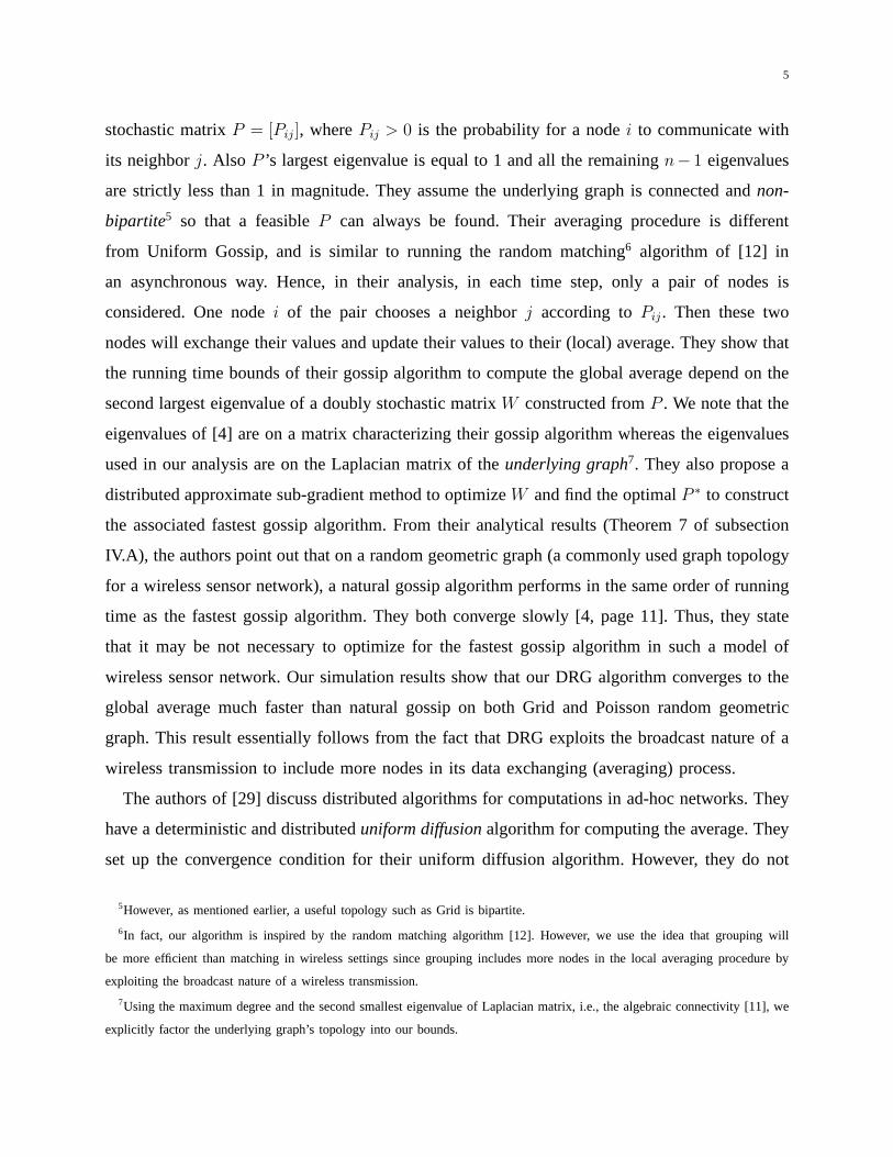
5

stochastic matrixP = [Pij ], wherePij > 0 is the probability for a nodei to communicate with

its neighborj. Also P ’s largest eigenvalue is equal to 1 and all the remainingn− 1 eigenvalues

are strictly less than 1 in magnitude. They assume the underlying graph is connected andnon-

bipartite5 so that a feasibleP can always be found. Their averaging procedure is different

from Uniform Gossip, and is similar to running the random matching6 algorithm of [12] in

an asynchronous way. Hence, in their analysis, in each time step, only a pair of nodes is

considered. One nodei of the pair chooses a neighborj according toPij . Then these two

nodes will exchange their values and update their values to their (local) average. They show that

the running time bounds of their gossip algorithm to computethe global average depend on the

second largest eigenvalue of a doubly stochastic matrixW constructed fromP . We note that the

eigenvalues of [4] are on a matrix characterizing their gossip algorithm whereas the eigenvalues

used in our analysis are on the Laplacian matrix of theunderlying graph7. They also propose a

distributed approximate sub-gradient method to optimizeW and find the optimalP ∗ to construct

the associated fastest gossip algorithm. From their analytical results (Theorem 7 of subsection

IV.A), the authors point out that on a random geometric graph(a commonly used graph topology

for a wireless sensor network), a natural gossip algorithm performs in the same order of running

time as the fastest gossip algorithm. They both converge slowly [4, page 11]. Thus, they state

that it may be not necessary to optimize for the fastest gossip algorithm in such a model of

wireless sensor network. Our simulation results show that our DRG algorithm converges to the

global average much faster than natural gossip on both Grid and Poisson random geometric

graph. This result essentially follows from the fact that DRG exploits the broadcast nature of a

wireless transmission to include more nodes in its data exchanging (averaging) process.

The authors of [29] discuss distributed algorithms for computations in ad-hoc networks. They

have a deterministic and distributeduniform diffusion algorithm for computing the average. They

set up the convergence condition for their uniform diffusion algorithm. However, they do not

5However, as mentioned earlier, a useful topology such as Grid is bipartite.

6In fact, our algorithm is inspired by the random matching algorithm [12]. However, we use the idea that grouping will

be more efficient than matching in wireless settings since grouping includes more nodes in the local averaging procedureby

exploiting the broadcast nature of a wireless transmission.

7Using the maximum degree and the second smallest eigenvalueof Laplacian matrix, i.e., the algebraic connectivity [11], we

explicitly factor the underlying graph’s topology into ourbounds.

6

give a bound on running time. They also find the optimal diffusion parameter for each node.

However, the execution of their algorithm needs global information such as maximum degree

or the eigenvalue of a topology matrix. Our DRG algorithms are purely local and do not need

any global information, although some global information is used (only) in our analysis.

Randomized gossiping in [20] can be used to compute the aggregates in arbitrary graph since

at the end of gossiping, all the nodes will know all others’ initial values. Every node can post-

process all the information it received to get the aggregates. The bound of running time is

O(n log3 n) in arbitrary directed graphs. However, this approach is notsuitable for resource-

constrained sensor networks, since the number of transmission messages growsexponentially.

Finally, we mention that there have been some works on flocking theory (e.g., [26]) in control

systems literature; however, the assumptions, details, and methodologies are very different from

the problem we address here.

III. OVERVIEW

A sensor network is abstracted as a connected undirected graph G(V, E) with all the sensor

nodes as the set of verticesV and all the bi-directional wireless communication links asthe

set of edgesE. This underlying graph can be arbitrary depending on the deployment of sensor

nodes.

Let each sensor nodei be associated with an initial observation or measurement value denoted

as v(0)

i (v(0)

i ∈ R). The assigned values over all vertices is a vectorv(0)

. Let v(k)i represent the

value of nodei after running our algorithms fork rounds. For simplicity of notation, we omit

the superscript when the specific round numberk doesn’t matter.

The goal is to compute (aggregate) functions such as average, sum, max, min etc. on the

vector of valuesv(0)

. In this paper, we present and analyze simple and efficient, robust, local,

distributed algorithms for the computation of these aggregates.

The main idea in our algorithm,random grouping is as follows. In each “round” of the

algorithm, every node independently becomes a group leaderwith probabilitypg and then invites

its neighbors to join the group. Then all members in a group update their values with the locally

derivedaggregate (average, maximum, minimum, etc) of the group. Through thisrandomized

process, we show that all values will progressively converge to the correct aggregate value (the

average, maximum, minimum, etc.). Our algorithm is distributed, randomized, and only uses local

7

communication. Each node makes decisions independently while all the nodes in the network

progressively move toward a consensus.

To measure the performance, we assume that nodes run DRG in synchronous time slots, i.e.,

rounds, so that we can quantify the running time. The synchronization among sensor nodes can

be achieved by applying the method in [8], for example. However, we note that synchronization

is not crucial to our approach and our algorithms will still work in an asynchronous setting,

although the analysis will be somewhat more involved.

Our main technical result gives an upper bound on the expected number of rounds needed for

all nodes running DRG Ave to converge to theglobal average. The upper bound is

O(1

γlog(

φ0

ε2)),

where the parameterγ directly relates to the properties of the graph, and the grouping probability

used by our randomized algorithm; andε is the desired accuracy (all nodes’ values need to

be within ε from the global average). The parameterφ0 represents the grand variance of the

initial value distribution. Briefly, the upper bound of running time is decided by graph topology,

grouping probability of our algorithm, accuracy requirement, and initial value distribution of

sensor nodes.

The upper bound on the expected number of rounds for computing the global maximum or

minimum is

O(1

γlog(

(1 − ρ)n

ρ)),

whereρ is the accuracy requirement for Max/Min problem (ρ is the ratio of nodes which donot

have the global Max/Min value to all nodes in the network). A bound for the expected number of

necessary transmissions can be derived by using the result of the bound on the expected running

time.

The rest of this paper is organized as follows. In section IV,we detail our distributed

random grouping algorithm. In section V we analyze the performance of the algorithm while

computing various aggregates such as average, max, and min.In section VI, we discuss practical

issues in implementing the algorithm. The extensive simulation results of our algorithm and the

comparison to other distributed approaches of aggregates computation in sensor network are

presented in section VII. Finally, we conclude in section VIII. A table for all the figures and

tables is provided in the appendix.

8

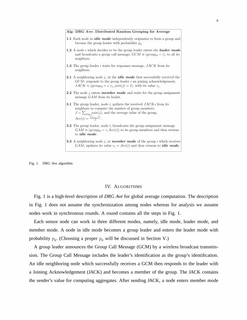
Alg: DRG Ave: Distributed Random Grouping for Average

1.1 Each node in idle mode independently originates to form a group andbecome the group leader with probability pg.

1.2 A node i which decides to be the group leader enters the leader mode

and broadcasts a group call message, GCM ≡ (groupid = i), to all itsneighbors.

1.3 The group leader i waits for responses message, JACK from itsneighbors.

2.1 A neighboring node j, at the idle mode that successfully received theGCM , responds to the group leader i an joining acknowledgement,JACK ≡ (groupid = i, vj, join(j) = 1), with its value vj.

2.2 The node j enters member mode and waits for the group assignmentmessage GAM from its leader.

3.1 The group leader, node i, gathers the received JACKs from itsneighbors to compute the number of group members,J =

∑

j∈gijoin(j), and the average value of the group,

Ave(i) =∑

k∈givk

J.

3.2 The group leader, node i, broadcasts the group assignment messageGAM ≡ (groupid = i, Ave(i)) to its group members and then returnsto idle mode .

3.3 A neighboring node j, at member mode of the group i which receivesGAM , updates its value vj = Ave(i) and then returns to idle mode .

Fig. 1. DRG Ave algorithm

IV. A LGORITHMS

Fig. 1 is a high-level description ofDRG Ave for global average computation. The description

in Fig. 1 does not assume the synchronization among nodes whereas for analysis we assume

nodes work in synchronous rounds. A round contains all the steps in Fig. 1.

Each sensor node can work in three different modes, namely, idle mode, leader mode, and

member mode. A node in idle mode becomes a group leader and enters the leader mode with

probability pg. (Choosing a properpg will be discussed in Section V.)

A group leader announces the Group Call Message (GCM) by a wireless broadcast transmis-

sion. The Group Call Message includes the leader’s identification as the group’s identification.

An idle neighboring node which successfully receives a GCM then responds to the leader with

a Joining Acknowledgement (JACK) and becomes a member of thegroup. The JACK contains

the sender’s value for computing aggregates. After sendingJACK, a node enters member mode

9

and will not response to any other GCMs until it returns to idle mode again. A member node

waits for the local aggregate from the leader to update its value. The leader gathers the group

members’ values from JACKs, computes the local aggregate (average of its group) and then

broadcasts it in the Group Assignment Message (GAM) by a wireless transmission. Member

nodes then update their values by the assigned value in the received GAM. Member nodes can

tell if the GAM is their desired one by the group identification in GAM.

TheDRG Max/Min algorithms to compute the maximum or minimum value of the network is

only a slight modification of the DRG Ave algorithm. Instead of broadcasting the local average

of the group, in the step 3, the group leader broadcasts the local maximum or minimum of the

group.

Note that only nodes in the idle mode will receive GCM and become a member of a group. A

node has received a GCM and entered the member mode will ignore the latter GCMs announced

by some other neighbors until it returns to the idle mode again. A node in leader node, of course,

will ignore the GCMs from its neighbors.

V. ANALYSIS

In this section we analyze the DRG algorithms by two performance measurement metrics:

expected running time and expected total number of transmissions. The number of total trans-

missions is a measurement of the energy cost of the algorithm. The running time will be measured

in the unit of a “round” which contains the three main steps inFig. 1.

Our analysis builds on the technique of [12] which analyzes aproblem of dynamic load

balancing by random matchings. In the load balancing problem, they deal with discrete values

(v ∈ In), but we deal with continuous values (v ∈ R

n) which makes our analysis different. Our

algorithm uses random groupings instead of random matchings. This has two advantages. The

first we show that the convergence is faster and hence faster running time and more importantly,

it is well-suited to the ad hoc wireless network setting because it is able to exploit the broadcast

nature of wireless communication.

To analyze our algorithm we need the concept of apotential function as defined below.

Definition 1: Consider an undirected connected graphG(V, E) with |V| = n nodes. Given

a value distributionv = [v1, ..., vn]T , vi is the value of nodei, the potential of the graphφ is

10

defined as

φ = ||v − vu||22 =∑

i∈V

(vi − v)2 = (∑

i∈V

v2i ) − nv2 (1)

wherev is the mean (global average) value over the network.

Thus,φ is a measurement of the grand variance of the value distribution. Note thatφ = 0 if

and only if v = vu, whereu = [1, 1, . . . , 1]T is the unit vector. We will use the notationφk to

denote the potential in roundk and useφ in general when specific round number doesn’t matter.

Let the potential decrement from a groupgi led by nodei after one round of the algorithm

be δφ|gi≡ δϕi,

δϕi =∑

j∈gi

v2j −

(∑

j∈givj)

2

J=

1

J

∑

j,k∈gi

(vj − vk)2, (2)

whereJ = |gi| is the number of members joining groupi (including the leader nodei). Since

each node joins at most one group in any round, throughout thealgorithm, the sum of all the

nodes’ values is maintained constant (equal to the initial sum of all nodes’ values). The property

δϕi ≥ 0 along with the fact that the total sum is invariant indicatesthat the value distributionv

will eventually converge to the average vectorvu by invoking our algorithm repeatedly.

For analysis, we assume that every node independently and simultaneously decides whether

to be a group leader or not at the beginning of a round. Those who decided to be leaders

will then send out their GCMs at the same time. Leaders’ neighbors who successfully receive

GCM will join their respective groups. We obtain our main analytic result, Theorem 2 — the

upper bound of running time — by bounding the expected decrement of the potentialE[δφ] of

each round. Welower bound E[δφ] by the sum ofE[δϕi] from all complete groups. A group

is a complete group if and only if the leader has all of its neighbors joining its group. In a

wireless setting, it is possible that a collision8 happens9 between two GCMs so that some nodes

8 It is also possible that a lower-level (MAC) layer protocol can resolve collisions amid GCMs so that a node in GCMs’

overlapping (collision) area can randomly choose one groupto join. (For correctness of the DRG Ave algorithm it is necessary

that a node joins at most one group in one round.) To analyze our algorithm in a general way (independent of the underlying

lower-level protocol), we consider onlycomplete groups (whose GCMs will have no collisions) to obtain an upper boundon

the convergence time. Our algorithm will work correctly whether there are collisions or not and makes no assumptions on the

lower-level protocol.

9For each node announcing GCM, a collision happens at probability 1− ps; Hereps is the probability that a GCM encounter

no collision.

11

h

k ji

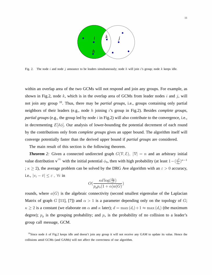
Fig. 2. The nodei and nodej announce to be leaders simultaneously; nodeh will join i’s group; nodek keeps idle.

within an overlap area of the two GCMs will not respond and join any groups. For example, as

shown in Fig.2, nodek, which is in the overlap area of GCMs from leader nodesi and j, will

not join any group10. Thus, there may bepartial groups, i.e., groups containing only partial

neighbors of their leaders (e.g., nodeh joining i’s group in Fig.2). Besidescomplete groups,

partial groups (e.g., the group led by nodei in Fig.2) will also contribute to the convergence, i.e.,

in decrementingE[δφ]. Our analysis of lower-bounding the potential decrement ofeach round

by the contributions only fromcomplete groups gives an upper bound. The algorithm itself will

converge potentially faster than the derived upper bound ifpartial groups are considered.

The main result of this section is the following theorem.

Theorem2: Given a connected undirected graphG(V, E), |V| = n and an arbitrary initial

value distributionv(0)

with the initial potentialφ0, then with high probability (at least1−( ε2

φ0)κ−1

; κ ≥ 2), the average problem can be solved by the DRG Ave algorithm with anε > 0 accuracy,

i.e., |vi − v| ≤ ε , ∀i in

O(κd log(φ0

ε2 )

pgps(1 + α)a(G))

rounds, wherea(G) is the algebraic connectivity (second smallest eigenvalueof the Laplacian

Matrix of graphG [11], [7]) and α > 1 is a parameter depending only on the topology ofG;

κ ≥ 2 is a constant (we elaborate onα andκ later);d = max (di)+1 ≈ max (di) (the maximum

degree);pg is the grouping probability; andps is the probability of no collision to a leader’s

group call message, GCM.

10Since nodek of Fig.2 keeps idle and doesn’t join any group it will not receive any GAM to update its value. Hence the

collisions amid GCMs (and GAMs) will not affect the correctness of our algorithm.

12

TABLE I

THE ALGEBRAIC CONNECTIVITY a(G) AND d/a(G), [12]

Graph a(G) d/a(G)

Clique n O(1)

d-regular expander Θ(d) O(1)

Grid Θ( 1n) O(n)

linear array Θ( 1n2 ) O(n2)

We note that, whenφ0 ≫ ε2 (which is typically the case), sayφ0 = Θ(n) and ε = O(1),

then DRG Ave converges to the global average with probability at least1 − 1/n in time

O(d log(

φ0ε2

)

pgps(1+α)a(G)).

Table I shows the algebraic connectivitya(G) and d/a(G) on several typical graphs. The

connectivity status of a graph is well characterized by algebraic connectivitya(G). For the two

extreme examples given in the Table, the algebraic connectivity of a clique (complete graph)

which is fully connected is much larger than that of a linear array which is least connected.

The parameterps, the probability that a GCM encounters no collision, is related topg and the

graph’s topology. Given a graph, increasingpg results in decreasingps, and vice versa. However,

there does exist a maximum value ofP = pg · ps, the probability for a node to form acomplete

group, so that we could have the best performance of DRG by a wise choice of pg. We will

discuss how to appropriately choosepg to maximizepgps later in subsection V-B after proving

the theorem.

For a pre-engineered deterministic graph (topology), suchasgrid, we can compute each node’s

ps according to the topology and therefore find the minimalps. The minimalps then is used

in Theorem 2. For arandom geometric graph, we can computeps according to its stochastic

node-distribution model. An example of derivingps on a Poisson random geometric graph is

shown in appendix I.

The proof and the discussions of Theorem 2 are presented in the following paragraphs.

13

(2) H

i

k k

ii

(3) C

(7) C(6) C(5) C(4) C

(1) G

k

h

i

k

h

hh h

l l l

lh

j

j

j

jj

k

i

i k j l

h

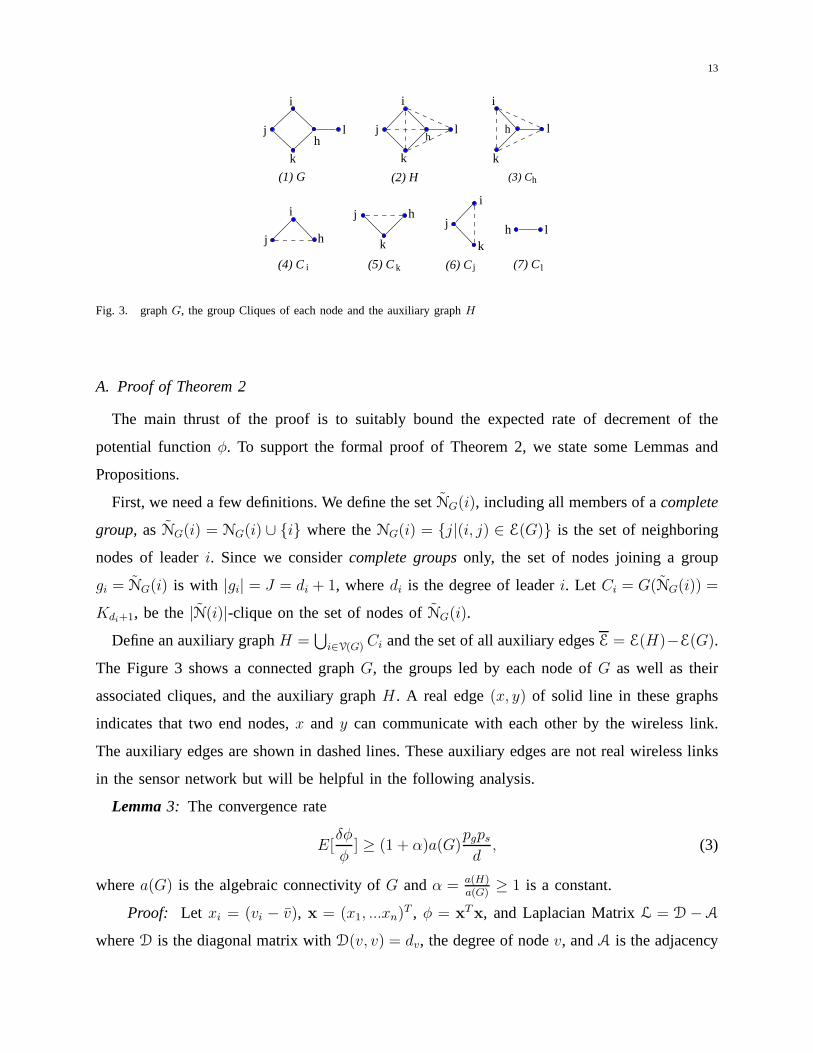
Fig. 3. graphG, the group Cliques of each node and the auxiliary graphH

A. Proof of Theorem 2

The main thrust of the proof is to suitably bound the expectedrate of decrement of the

potential functionφ. To support the formal proof of Theorem 2, we state some Lemmas and

Propositions.

First, we need a few definitions. We define the setNG(i), including all members of acomplete

group, asNG(i) = NG(i) ∪ i where theNG(i) = j|(i, j) ∈ E(G) is the set of neighboring

nodes of leaderi. Since we considercomplete groups only, the set of nodes joining a group

gi = NG(i) is with |gi| = J = di + 1, wheredi is the degree of leaderi. Let Ci = G(NG(i)) =

Kdi+1, be the|N(i)|-clique on the set of nodes ofNG(i).

Define an auxiliary graphH =⋃

i∈V(G) Ci and the set of all auxiliary edgesE = E(H)−E(G).

The Figure 3 shows a connected graphG, the groups led by each node ofG as well as their

associated cliques, and the auxiliary graphH. A real edge(x, y) of solid line in these graphs

indicates that two end nodes,x and y can communicate with each other by the wireless link.

The auxiliary edges are shown in dashed lines. These auxiliary edges are not real wireless links

in the sensor network but will be helpful in the following analysis.

Lemma3: The convergence rate

E[δφ

φ] ≥ (1 + α)a(G)

pgps

d, (3)

wherea(G) is the algebraic connectivity ofG andα = a(H)a(G)

≥ 1 is a constant.

Proof: Let xi = (vi − v), x = (x1, ...xn)T , φ = xT x, and Laplacian MatrixL = D − A

whereD is the diagonal matrix withD(v, v) = dv, the degree of nodev, andA is the adjacency

14

matrix of the graph.LG andLH are the Laplacian Matrices of graphG andH respectively.

Let ∆jk = (vj − vk)2 = (xj − xk)

2; ps be the probability for a node to announce the GCM

without collision, andd = max (di)+1, wheredi is the degree of nodei. The expected decrement

of the potential in the whole network is

E[δφ] = E[∑

i∈V

δϕi ] ≥ pgps

∑

i∈V

δϕi

= pgps

∑

i∈V

1

di + 1

∑

(j,k)∈E(Ci)

∆jk

≥ pgps

1

d

∑

i∈V

∑

(j,k)∈E(Ci)

∆jk

= pgps

1

d

∑

i∈V

∑

(j,k)∈E(Ci)

(xj − xk)2

(a)≥

pgps

1

d(

∑

(j,k)∈E(G)

2(xj − xk)2 +

∑

(j,k)∈E

(xj − xk)2)

= pgps

1

d(

∑

(j,k)∈E(G)

(xj − xk)2 +

∑

(j,k)∈E(H)

(xj − xk)2)

= pgps

1

d(xT

LGx + xTLHx). (4)

Here (a) follows from the fact that for each edge(i, j) ∈ E, ∆ij appears at least twice in the

sumE[δφ]. Also each auxiliary edge(j, k) ∈ E contributes at least once.

E[δφ

φ] ≥ pgps

1

d(xT LGx + xT LHx

xT x)

≥ pgps

1

d(min

x

(xT LGx

xTx|x⊥u,x 6= 0) + min

x

(xT LHx

xTx|x⊥u,x 6= 0))

= pgps

1

d(a(G) + a(H)) = (1 + α)a(G)

pgps

d(5)

, where α =a(H)

a(G).

In the above, we exploit the Courant-Fischer Minimax Theorem [7]:

a(G) = λ2 = minx

(xT LGx

xTx|x⊥u,x 6= 0). (6)

SinceH is always denser thanG, according to Courant-Weyl Inequalities,α ≥ 1 [7].

For convenience, we denote

γ = (1 + α)a(G)pgps

d. (7)

15

Lemma4: Let the conditional expectation value ofφτ computed over all possible group

distributions in roundτ , given an group distribution with the potentialφτ−1 in the previous

roundτ −1, is Eaτ[φτ ]. Here we denote thea1, a2, . . . , aτ as the independent random variables

representing the possible group distributions happening at rounds1, 2, . . . , τ, respectively. Then,

the E[φτ ] = Ea1,a2,...,aτ[φτ ] ≤ (1 − γ)τφ0.

Proof: From the Lemma 3, the

Eak[φk] ≤ (1 − γ)φk−1

and by the definition,

E[φk] = Ea1,a2,...,ak[φk]

= Ea1 [Ea2 [· · ·Eak−1[Eak

[φk]] · · · ]]

≤ (1 − γ)Ea1 [Ea2 [· · ·Eak−1[φk−1] · · · ]]

......

≤ (1 − γ)kφ0. (8)

The next proposition relates the potential to the accuracy criterion.

Proposition5: Let φτ be the potential right after theτ -th round of the DRG Ave algorithm,

if φτ ≤ ε2, then the consensus has been reached at or before theτ -th round.

(the potential of theτ -th roundφτ ≤ ε2 ⇒ |v(τ)

i − v| ≤ ε, ∀i)

Proof: The vi and v in the following are the value on nodei and the average value over

the network respectively, right after roundτ .

∵ (vi − v)2 ≥ 0, ∀i ∈ V(G) (9)

∴ φτ =∑

i∈V(G)

(vi − v)2 ≤ ε2 ⇒ (vi − v)2 ≤ ε2 (10)

⇔ |vi − v| ≤ ε, ∀i ∈ V(G)). (11)

The proof of Theorem 2: Now we finish the proof of our main theorem.

Proof: By Lemma 4 and Proposition 5,

E[φτ ] ≤ (1 − γ)τφ0 ≤ ε2. (12)

16

Taking logarithm on the two right terms,

τ log(1

1 − γ) ≥ log φ0 − log ε2 (13)

τ ≥log(φ0

ε2 )

log( 11−γ

)≈

1

γlog(

φ0

ε2) (14)

Also, φ0 > ε2 (in fact, φ0 ≫ ε2 sinceφ0 = θ(n), ε2 = O(1) and so ε2

φ0= O( 1

n)), otherwise the

accuracy criterion is trivially satisfied. By Markov inequality

Pr(φτ > ε2) <E[φτ ]

ε2≤

(1 − γ)τφ0

ε2(15)

Chooseτ = κγ

log(φ0

ε2 ) where theκ ≥ 2. Then because( ε2

φ0) ≪ 1 and (κ − 1) ≥ 1,

P r(φτ > ε2) <(1 − γ)

κγ

log(φ0ε2

)φ0

ε2≤ e− log(

φ0ε2

)κ φ0

ε2

= (ε2

φ0)(κ−1) −→ 0, (16)

∵ε2

φ0

≪ 1 and (κ − 1) ≥ 1.

Thus,Pr(φτ ≤ ε2) ≥ 1− ( ε2

φ0)(κ−1). (Since typicallyφ0 ≫ ε2, takingκ = 2 is sufficient to have

high probability at least1 − O( 1n); in caseφ0 > ε2, then a largerκ is needed to have a high

probability). From (16), with high probabilityφτ ≤ ε2 when τ = O(κγ

log φ0

ε2 ), by proposition 5

the accuracy criterion must have been reached at or before the τ -th round.

B. Discussion of the upper bound in Theorem 2

As mentioned earlier,ps is related topg and the topology of the underlying graph. For example,

in a Poisson random geometric graph [27], in which the location of each sensor node can

be modeled by a 2-D homogeneous Poisson point process with intensity λ, ps = e−λ·pg·4πr2

(please see the appendix I for the detail deriving process),wherer is the transmission range.

We assume that sensor nodes are deployed in anunit area, so thatλ is equal ton. To maintain

the connectivity, we set4πr2 = z(n)n

= 4 log(n)+log(log(n))n

[14]. Let P = pgps. The maximum of

P = pge−pg·z(n), denoted asP, happens atpg = 1

z(n)= 1

4(log(n)+log(log(n)))where dP

dpg= 0. The

maximumP ≃ 14d

e−1.

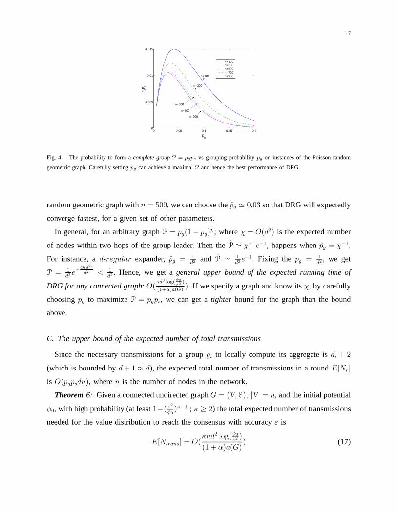
Fig.4 shows the curves ofpgps on Poisson random geometric graphs withn varying from

100 to 900. It is easy to find a good value ofpg in these graphs. For instance, given a Poisson

17

0 0.05 0.1 0.15 0.20

0.005

0.01

0.015

pg

p gp s

n=100n=300n=500n=700n=900n=100

n=300

n=500

n=700

n=900

Fig. 4. The probability to form acomplete group P = pgps vs grouping probabilitypg on instances of the Poisson random

geometric graph. Carefully settingpg can achieve a maximalP and hence the best performance of DRG.

random geometric graph withn = 500, we can choose thepg ≃ 0.03 so that DRG will expectedly

converge fastest, for a given set of other parameters.

In general, for an arbitrary graphP = pg(1− pg)χ; whereχ = O(d2) is the expected number

of nodes within two hops of the group leader. Then theP ≃ χ−1e−1, happens whenpg = χ−1.

For instance, ad-regular expander,pg = 1d2 and P ≃ 1

d2 e−1. Fixing the pg = 1

d2 , we get

P = 1d2 e

−O(d2)

d2 < 1d2 . Hence, we get ageneral upper bound of the expected running time of

DRG for any connected graph: O(κd3 log(

φ0ε2

)

(1+α)a(G)). If we specify a graph and know itsχ, by carefully

choosingpg to maximizeP = pgps, we can get atighter bound for the graph than the bound

above.

C. The upper bound of the expected number of total transmissions

Since the necessary transmissions for a groupgi to locally compute its aggregate isdi + 2

(which is bounded byd + 1 ≈ d), the expected total number of transmissions in a roundE[Nr]

is O(pgpsdn), wheren is the number of nodes in the network.

Theorem6: Given a connected undirected graphG = (V, E), |V| = n, and the initial potential

φ0, with high probability (at least1−( ε2

φ0)κ−1 ; κ ≥ 2) the total expected number of transmissions

needed for the value distribution to reach the consensus with accuracyε is

E[Ntrans] = O(κnd2 log(φ0

ε2 )

(1 + α)a(G)) (17)

18

Proof:

E[Ntrans] = E[Nr]O(κd log(φ0

ε2 )

pgps(1 + α)a(G)) = O(

κnd2 log(φ0

ε2 )

(1 + α)a(G)) (18)

D. DRG Max/Min algorithms

Instead of announcing the local average of a group, the groupleader in the DRG Max/Min

algorithm announces the local Max/Min of a group. Then all the members of a group update

their values to the local Max/Min. Since the global Max/Min is also the local Max/Min, the

global Max/Min value will progressively replace all the other values in the network.

In this subsection, we analyze the running time of DRG Max/Min algorithms by using the

analytical results of the DRG Ave algorithm. However, for the Max/Min we need a different

accuracy criterion:ρ = n−mn

, wheren, m is the total number of nodes and the number of nodes of

the global Max/Min, respectively.ρ indicates the proportion of nodes that havenot yet changed

to the global Max/Min. When a small enoughρ is satisfied after running DRG Max/Min, with

high probability (1 − ρ), a randomly chosen node is of the global Max/Min.

We only need to consider Max problem since Min problem is symmetric to the Max problem.

Moreover, we assume there is only one global Max valuevmax in the network. This is the worst

situation. If there is more than one node with the samevmax in the network then the network

will reach consensus faster because there is more than one “diffusion” source.

Theorem7: Given a connected undirected graphG(V, E), |V| = n and an arbitrary initial

value distributionv(0)

, then with high probability (at least1− ( ρ

(1−ρ)n)κ−1 ; κ ≥ 2) the Max/Min

problem can be solved under the desired accuracy criterionρ, after invoking the DRG Max/Min

Algorithm

O(κ

γlog(

(1 − ρ)n

ρ))

times, where theγ = Ω((1 + α)a(G)pgps

d).

Proof: The proof is based on two facts: (1) The expected running timeof the DRG Max/Min

algorithm on an arbitrary initial value distributionv(0)

a = [v1, . . . , vi−1, vi = vmax, vi+1 . . . , vn]T

will be exactly the same as that on the binary initial distributionv(0)

b = [0, . . . , 0, vi = 1, 0, . . . 0]T

under the same accuracy criterionρ. The vmax in v(0)

a will progressively replace all the other

values no matter what the replaced values are. We can map thevmax to “1” and all the others

19

to “0”. Therefore, we only need to consider the special binary initial distribution v(0)

b in the

following analysis. (2) Suppose the DRG Ave and DRG Max algorithms are running on the

same binary initial distributionv(0)

b and going through the same grouping scenario which means

that the two algorithms encounter the same group distribution in every round. Under the same

grouping scenario, in each round, those nodes of non-zero value in DRG Ave are of the maximum

valuevmax in DRG Max.

Based on these two facts, a relationship between two algorithms’ accuracy criteria:ε2 = ρ

(1−ρ)n,

can be exploited to obtain the upper bound of expected running time of DRG Max algorithm

from that of DRG Ave algorithm. Now we present our analysis indetail.

We run two algorithms on the same initial value distributionv(0)

b and go through the same sce-

nario. To distinguish their value distributions after, sayζ rounds, we denote the value distribution

for DRG Ave asv(ζ)

≡ v(ζ)

b |DRG Ave and that for DRG Max asw(ζ)

≡ v(ζ)

b |DRG Max.

Without loss of generality, supposew(ζ)

= [w1 = 1, . . . , wm = 1, wm+1 = 0, . . . , wn = 0]T .

There arem “1”s and (n − m) “0”s. Then the correspondingv(ζ)

= [v1, v2, . . . vm, vm+1 =

0, . . . , vn = 0]T . Apparentlywi = ⌈vi⌉. Although the values fromvm+1 to vn are still “0”s, the

values fromv1 to vm could be any value∈ (0, 1). To bound the running time, we need to know

the potentialφζ , which now is a random variable at theζ-th round. We now calculate a bound

on the minimum value for the potentialφζ.

The minimum value of the potentialφζ at theζ- round with exactlym non-zero values is a

simple optimization problem formulated as follows:

min∑

i∈V(G)

(vi − v)2

subject tom

∑

i=1

vi − 1 = 0 (19)

1 ≥ vi > 0; 1 ≤ i ≤ m,

vi = 0; m < i ≤ n.

wheren = |V(G)| andv = 1n.

By the Lagrange Multiplier Theorem, the minimum happens at

v∗i =

1m

1 ≤ i ≤ m.

0 otherwise.(20)

20

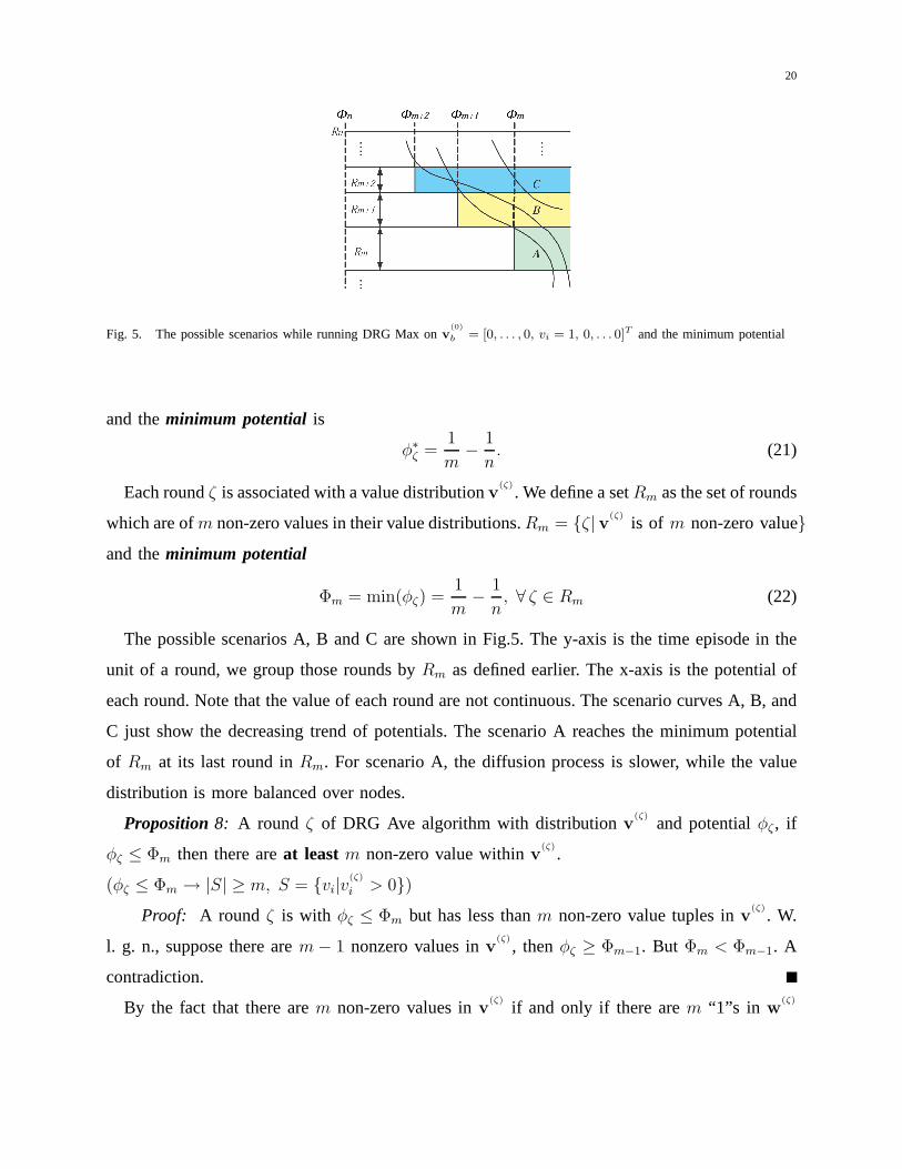
Fig. 5. The possible scenarios while running DRG Max onv

(0)

b = [0, . . . , 0, vi = 1, 0, . . . 0]T and the minimum potential

and theminimum potential is

φ∗ζ =

1

m−

1

n. (21)

Each roundζ is associated with a value distributionv(ζ)

. We define a setRm as the set of rounds

which are ofm non-zero values in their value distributions.Rm = ζ |v(ζ)

is of m non-zero value

and theminimum potential

Φm = min(φζ) =1

m−

1

n, ∀ ζ ∈ Rm (22)

The possible scenarios A, B and C are shown in Fig.5. The y-axis is the time episode in the

unit of a round, we group those rounds byRm as defined earlier. The x-axis is the potential of

each round. Note that the value of each round are not continuous. The scenario curves A, B, and

C just show the decreasing trend of potentials. The scenarioA reaches the minimum potential

of Rm at its last round inRm. For scenario A, the diffusion process is slower, while the value

distribution is more balanced over nodes.

Proposition8: A round ζ of DRG Ave algorithm with distributionv(ζ)

and potentialφζ, if

φζ ≤ Φm then there areat least m non-zero value withinv(ζ)

.

(φζ ≤ Φm → |S| ≥ m, S = vi|v(ζ)

i > 0)

Proof: A round ζ is with φζ ≤ Φm but has less thanm non-zero value tuples inv(ζ)

. W.

l. g. n., suppose there arem − 1 nonzero values inv(ζ)

, thenφζ ≥ Φm−1. But Φm < Φm−1. A

contradiction.

By the fact that there arem non-zero values inv(ζ)

if and only if there arem “1”s in w(ζ)

21

and by proposition 8, we can set

Φm = ε2 =1

m−

1

n=

ρ

(1 − ρ)n. (23)

For the distributionv(0)

b which we are dealing with, the initial potentialφ0 = 1 − 1n≈ 1. Thus,

substituting ρ

(1−ρ)nfor ε2 in Theorem 2, we get the upper bound of the expected running time

of DRG Max algorithm to reach a desired accuracy criterionρ = n−mn

, which is

O(κ

γlog(

(1 − ρ)n

ρ)).

The γ follows the rules mentioned before.

The upper bound of the expected number of the total necessarytransmissions for DRG Max

is

E[Ntrans] = O(κnd2 log( (1−ρ)n

ρ)

(1 + α)a(G)) (24)

by the same deriving process of Theorem 6.

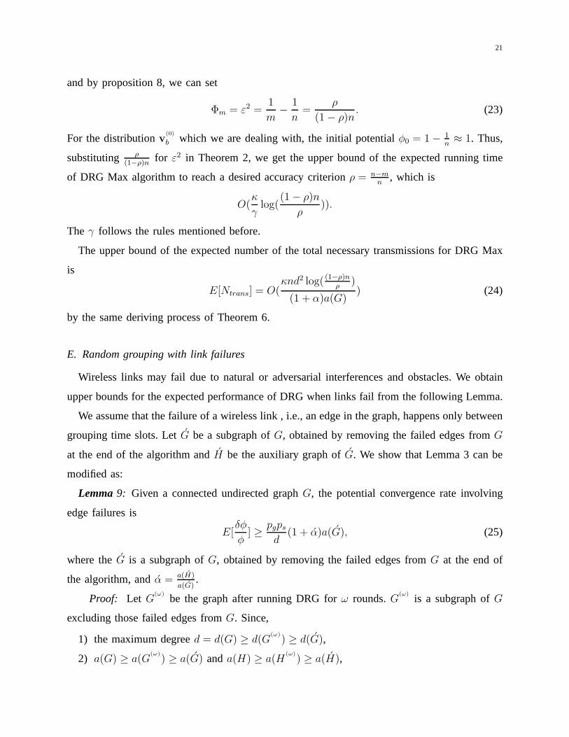
E. Random grouping with link failures

Wireless links may fail due to natural or adversarial interferences and obstacles. We obtain

upper bounds for the expected performance of DRG when links fail from the following Lemma.

We assume that the failure of a wireless link , i.e., an edge inthe graph, happens only between

grouping time slots. LetG be a subgraph ofG, obtained by removing the failed edges fromG

at the end of the algorithm andH be the auxiliary graph ofG. We show that Lemma 3 can be

modified as:

Lemma9: Given a connected undirected graphG, the potential convergence rate involving

edge failures is

E[δφ

φ] ≥

pgps

d(1 + α)a(G), (25)

where theG is a subgraph ofG, obtained by removing the failed edges fromG at the end of

the algorithm, andα = a(H)

a(G).

Proof: Let G(ω)

be the graph after running DRG forω rounds.G(ω)

is a subgraph ofG

excluding those failed edges fromG. Since,

1) the maximum degreed = d(G) ≥ d(G(ω)

) ≥ d(G),

2) a(G) ≥ a(G(ω)

) ≥ a(G) anda(H) ≥ a(H(ω)

) ≥ a(H),

22

we have

E[δφ

(k)

φ(k)] ≥

pgps

d(G(k))(a(G

(k)

) + a(H(k)

)) ≥pgps

d(a(G) + a(H)) =

pgps

d(1 + α)a(G). (26)

By Lemma 9, we obtain the modified convergence rateγ = pgps

d(1 + α)a(G). Replacingγ by

γ we have the upper bounds on the performance of DRG in case of edge failures.

VI. PRACTICAL CONSIDERATIONS

A practical issue is deciding when nodes should stop the DRG iterations of a particular

aggregate computation. An easy way to stop, as in [18], is to let the node which initiates the

aggregate query disseminate a stop message to cease the computation. The querying node samples

and compares the values from different nodes located at different locations. If the sampled values

are all the same or within some satisfiable accuracy range, the querying node disseminates the

stop messages. This method incurs a delay overhead on the dissemination.

A purely distributed local stop mechanism on each node is also desirable. The related distrib-

uted algorithms [4], [12], [18], [29] all fail to have such a local stop mechanism. However, nodes

running our DRG algorithms can stop the computation locally. The purely local stop mechanism

is to adapt the grouping probabilitypg to the value change. If in consecutive rounds, the value

of a node remains the same or just changes within a very small range, the node reduces its

own grouping probabilitypg accordingly. When a node meets the accuracy criterion, it can stay

idle. However, in future, the node can still join a group called by its neighbor. If the value

changes again by a GAM, Group Assignment Message, from one ofits neighbors, its grouping

probability increases accordingly to actively re-join theaggregate computation process. We leave

the detail of this implementation for future work.

Considering correlation among values of neighboring nodesin the aggregate computation [9]

may be useful but there may be some overhead to obtain or compute the “extra” correlation

information. In this paper, however, our goal was to study performance without any assumption

on the input values (can be arbitrary). One can presumably dobetter by making use of correlation.

Including correlation will be an extension to our current work.

23

0 10

1degree: min=1, max=11, ave=6.34

(a) 100 nodes topology I

0 10

1

degree: min=1, max=12, ave=6.22

(b) 100 nodes topology II

0 10


(c) 150 nodes

0 10


(d) 200 nodes

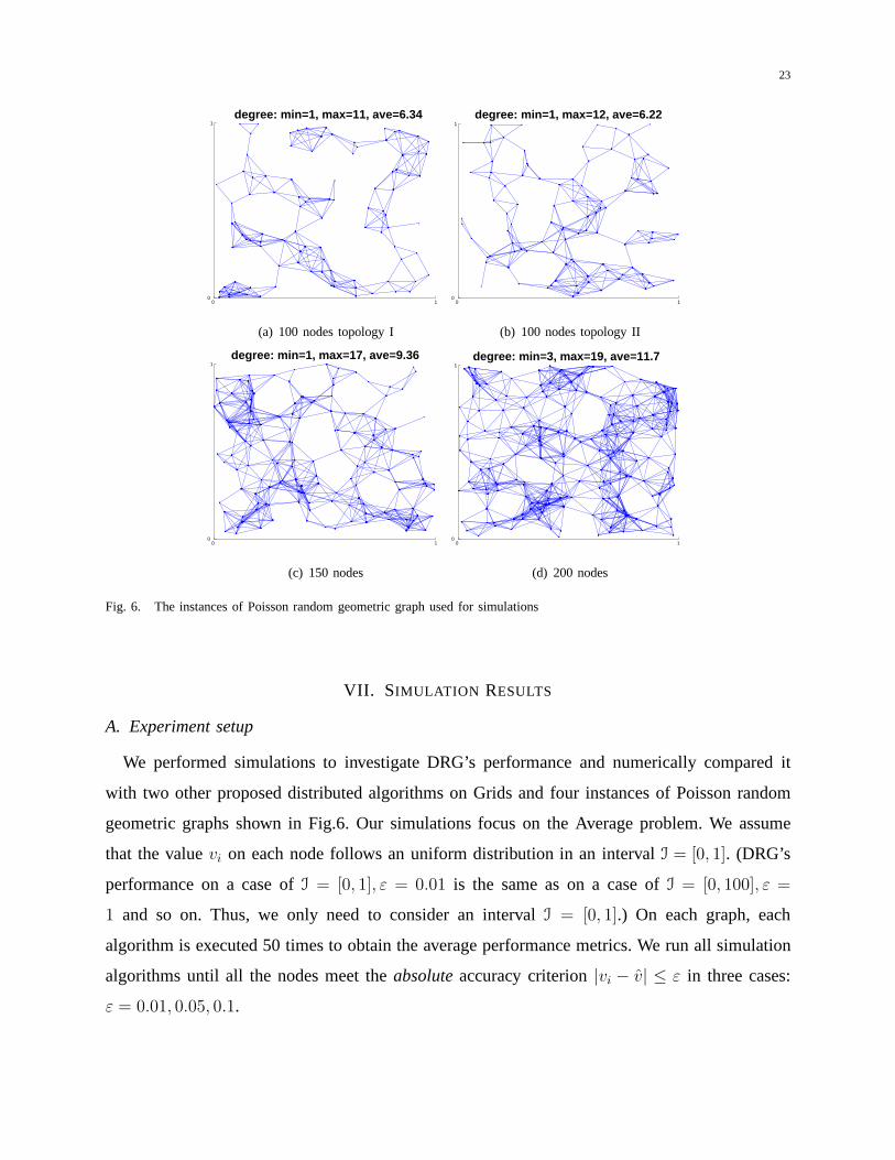
Fig. 6. The instances of Poisson random geometric graph usedfor simulations

VII. SIMULATION RESULTS

A. Experiment setup

We performed simulations to investigate DRG’s performanceand numerically compared it

with two other proposed distributed algorithms on Grids andfour instances of Poisson random

geometric graphs shown in Fig.6. Our simulations focus on the Average problem. We assume

that the valuevi on each node follows an uniform distribution in an intervalI = [0, 1]. (DRG’s

performance on a case ofI = [0, 1], ε = 0.01 is the same as on a case ofI = [0, 100], ε =

1 and so on. Thus, we only need to consider an intervalI = [0, 1].) On each graph, each

algorithm is executed 50 times to obtain the average performance metrics. We run all simulation

algorithms until all the nodes meet theabsolute accuracy criterion|vi − v| ≤ ε in three cases:

ε = 0.01, 0.05, 0.1.

24

0.010.05

0.18^210^213^215^220^2

0

100

200

300

400

500

εGrid size n=k 2

# ro

unds

ε=0.01ε=0.05ε=0.1

(a) Running time on Grid

0.010.05

0.18^210^2

13^215^2

20^2

0

2

4

6

8

10

x 104

εGrid size n=k 2

# tr

ansm

issi

ons ε=0.01

ε=0.05ε=0.1

(b) Total number of transmissions on Grid

0.010.05

0.1100(I)100(II)

150200

0

200

400

600

800

1000

ε# node −(topology)

# ro

unds

ε=0.01ε=0.05ε=0.1

(c) Running time on Poisson random geometric

graph

0.010.05

0.1100(I)100(II)

150200

0

1

2

3

4

5

x 104

ε# node (topology)

# tr

ansm

issi

ons

ε=0.01ε=0.05ε=0.1

(d) Total number of transmissions on Poisson ran-

dom geometric graph

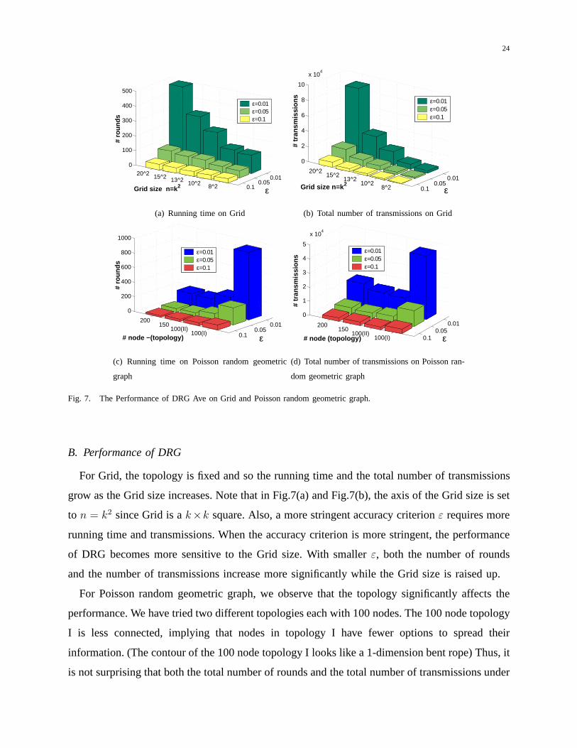
Fig. 7. The Performance of DRG Ave on Grid and Poisson random geometric graph.

B. Performance of DRG

For Grid, the topology is fixed and so the running time and the total number of transmissions

grow as the Grid size increases. Note that in Fig.7(a) and Fig.7(b), the axis of the Grid size is set

to n = k2 since Grid is ak×k square. Also, a more stringent accuracy criterionε requires more

running time and transmissions. When the accuracy criterion is more stringent, the performance

of DRG becomes more sensitive to the Grid size. With smallerε, both the number of rounds

and the number of transmissions increase more significantlywhile the Grid size is raised up.

For Poisson random geometric graph, we observe that the topology significantly affects the

performance. We have tried two different topologies each with 100 nodes. The 100 node topology

I is less connected, implying that nodes in topology I have fewer options to spread their

information. (The contour of the 100 node topology I looks like a 1-dimension bent rope) Thus, it

is not surprising that both the total number of rounds and thetotal number of transmissions under

25

topology I are much higher than those under topology II. In fact, the rounds and transmissions

needed on 100-node topology I are even higher than on the instances of 150 nodes and 200

nodes in Fig.6. The two instances of 150 and 200 nodes are wellconnected and similar to the

100 nodes topology II. These results match our analysis where the parameters in the upper bound

include not only the number of nodesn and grouping probabilitypg, but also the parameters

characterizing the topology — the maximum degreed and the algebraic connectivitya(G).

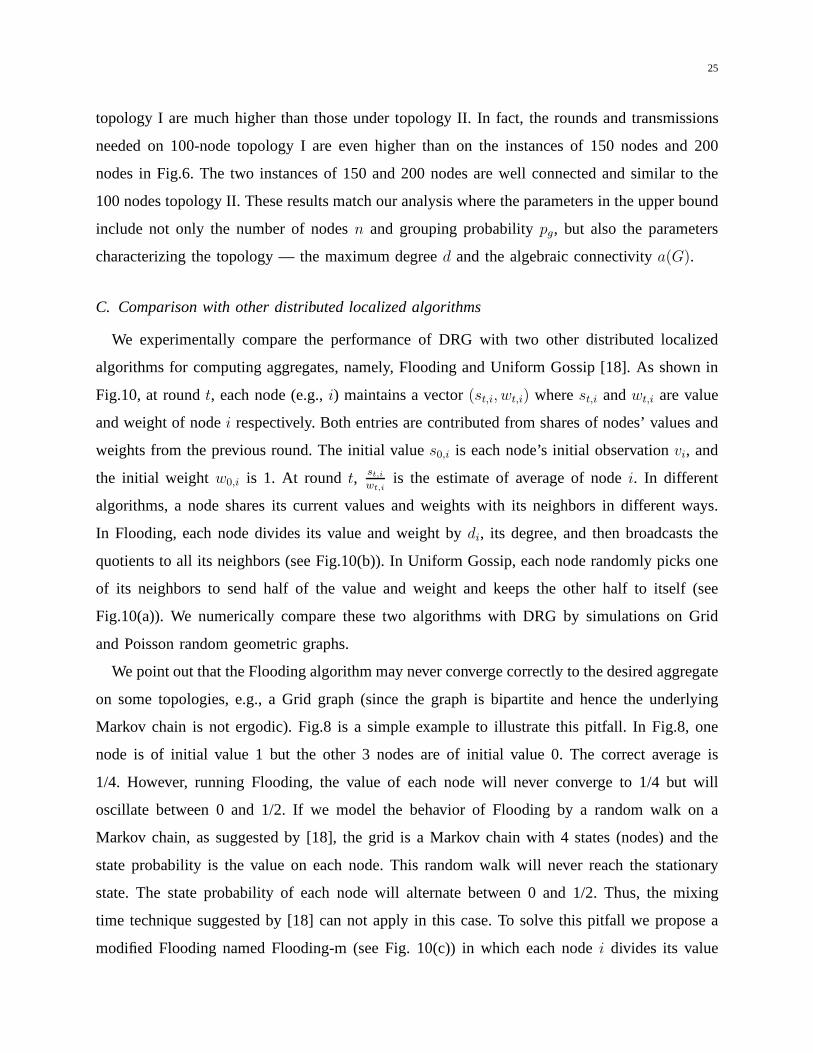
C. Comparison with other distributed localized algorithms

We experimentally compare the performance of DRG with two other distributed localized

algorithms for computing aggregates, namely, Flooding andUniform Gossip [18]. As shown in

Fig.10, at roundt, each node (e.g.,i) maintains a vector(st,i, wt,i) wherest,i andwt,i are value

and weight of nodei respectively. Both entries are contributed from shares of nodes’ values and

weights from the previous round. The initial values0,i is each node’s initial observationvi, and

the initial weightw0,i is 1. At roundt, st,i

wt,iis the estimate of average of nodei. In different

algorithms, a node shares its current values and weights with its neighbors in different ways.

In Flooding, each node divides its value and weight bydi, its degree, and then broadcasts the

quotients to all its neighbors (see Fig.10(b)). In Uniform Gossip, each node randomly picks one

of its neighbors to send half of the value and weight and keepsthe other half to itself (see

Fig.10(a)). We numerically compare these two algorithms with DRG by simulations on Grid

and Poisson random geometric graphs.

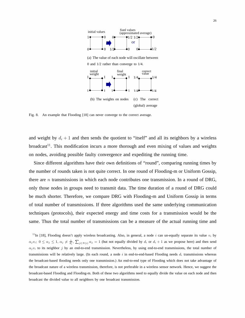
We point out that the Flooding algorithm may never converge correctly to the desired aggregate

on some topologies, e.g., a Grid graph (since the graph is bipartite and hence the underlying

Markov chain is not ergodic). Fig.8 is a simple example to illustrate this pitfall. In Fig.8, one

node is of initial value 1 but the other 3 nodes are of initial value 0. The correct average is

1/4. However, running Flooding, the value of each node will never converge to 1/4 but will

oscillate between 0 and 1/2. If we model the behavior of Flooding by a random walk on a

Markov chain, as suggested by [18], the grid is a Markov chainwith 4 states (nodes) and the

state probability is the value on each node. This random walkwill never reach the stationary

state. The state probability of each node will alternate between 0 and 1/2. Thus, the mixing

time technique suggested by [18] can not apply in this case. To solve this pitfall we propose a

modified Flooding named Flooding-m (see Fig. 10(c)) in whicheach nodei divides its value

26

(approximated average)

or1/20

0

1 0

0 1/20 1/20

1/2

fianl valuesinitial values

0

(a) The value of each node will oscillate between

0 and 1/2 rather than converge to 1/4.

1

1111

1weight

1 1weightfinalinitial

(b) The weights on nodes

1/4

1/4

1/4

1/4valuecorrect

(c) The correct

(global) average

Fig. 8. An example that Flooding [18] can never converge to the correct average.

and weight bydi + 1 and then sends the quotient to “itself” and all its neighborsby a wireless

broadcast11. This modification incurs a more thorough and even mixing of values and weights

on nodes, avoiding possible faulty convergence and expediting the running time.

Since different algorithms have their own definitions of “round”, comparing running times by

the number of rounds taken is not quite correct. In one round of Flooding-m or Uniform Gossip,

there aren transmissions in which each node contributes one transmission. In a round of DRG,

only those nodes in groups need to transmit data. The time duration of a round of DRG could

be much shorter. Therefore, we compare DRG with Flooding-m and Uniform Gossip in terms

of total number of transmissions. If three algorithms used the same underlying communication

techniques (protocols), their expected energy and time costs for a transmission would be the

same. Thus the total number of transmissions can be a measureof the actual running time and

11In [18], Flooding doesn’t apply wireless broadcasting. Also, in general, a nodei can un-equally separate its valuevi by

αjvi; 0 ≤ αj ≤ 1, αj 6= 1di

,P

j∈N(i) αj = 1 (but not equally divided bydi or di + 1 as we propose here) and then send

αjvi to its neighborj by an end-to-end transmission. Nevertheless, by using end-to-end transmissions, the total number of

transmissions will be relatively large. (In each round, a node i in end-to-end-based Flooding needsdi transmissions whereas

the broadcast-based flooding needs only one transmission.)An end-to-end type of Flooding which does not take advantageof

the broadcast nature of a wireless transmission, therefore, is not preferable in a wireless sensor network. Hence, we suggest the

broadcast-based Flooding and Flooding-m. Both of these twoalgorithms need to equally divide the value on each node and then

broadcast the divided value to all neighbors by one broadcast transmission.

27

energy consumption.

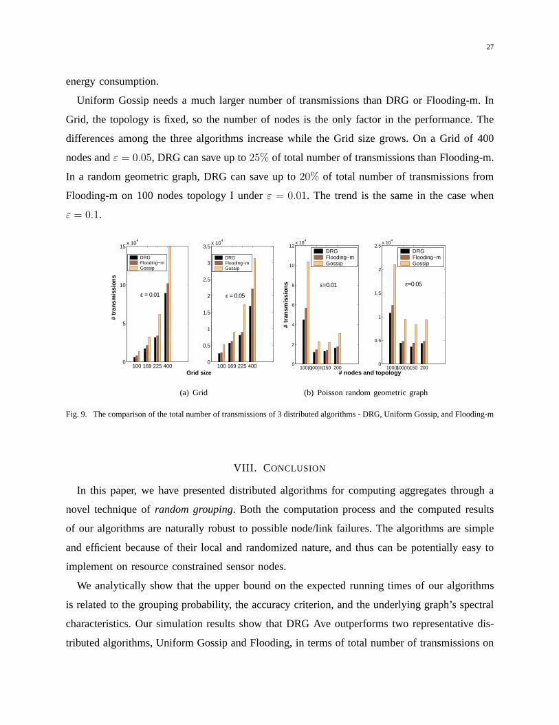
Uniform Gossip needs a much larger number of transmissions than DRG or Flooding-m. In

Grid, the topology is fixed, so the number of nodes is the only factor in the performance. The

differences among the three algorithms increase while the Grid size grows. On a Grid of 400

nodes andε = 0.05, DRG can save up to25% of total number of transmissions than Flooding-m.

In a random geometric graph, DRG can save up to20% of total number of transmissions from

Flooding-m on 100 nodes topology I underε = 0.01. The trend is the same in the case when

ε = 0.1.

100 169 225 4000

5

10

15x 10

4

ε = 0.01

Grid size

# tr

ansm

issi

ons

DRGFlooding−mGossip

100 169 225 4000

0.5

1

1.5

2

2.5

3

3.5x 10

4

ε = 0.05


(a) Grid

100(I)100(II)150 2000

2

4

6

8

10

12x 10

4

# nodes and topology

# tr

ansm

issi

ons


100(I)100(II)150 2000

0.5

1

1.5

2

2.5x 10

4


ε=0.01 ε=0.05

(b) Poisson random geometric graph

Fig. 9. The comparison of the total number of transmissions of 3 distributed algorithms - DRG, Uniform Gossip, and Flooding-m

VIII. C ONCLUSION

In this paper, we have presented distributed algorithms forcomputing aggregates through a

novel technique ofrandom grouping. Both the computation process and the computed results

of our algorithms are naturally robust to possible node/link failures. The algorithms are simple

and efficient because of their local and randomized nature, and thus can be potentially easy to

implement on resource constrained sensor nodes.

We analytically show that the upper bound on the expected running times of our algorithms

is related to the grouping probability, the accuracy criterion, and the underlying graph’s spectral

characteristics. Our simulation results show that DRG Ave outperforms two representative dis-

tributed algorithms, Uniform Gossip and Flooding, in termsof total number of transmissions on

28

Alg: Uniform Gossip

1 Initial: each node, e.g. node i sends (s0,i = vi, w0,i = 1) to itself.

2 Let (sr, wr) be all pairs sent to i in round t − 1.

3 Let st,i =∑

r sr; wt,i =∑

r wr.

4 i chooses one of its neighboring node j uniformly at random

5 i sends the pair (st,i

2,

wt,i

2) to j and itself.

6st,i

wt,iis the estimate of the average at node i of round t

(a) The Uniform Gossip algorithm

Alg: Flooding



3 Let st,i =∑

r sr; wt,i =∑

r wr.

4 broadcast the pair (st,i

di,

wt,i

di) to all neighboring nodes.

5st,i


(b) The broadcast-based Flooding algorithm

Alg: modified Flooding-m



3 Let st,i =∑

r sr; wt,i =∑

r wr.

4 broadcast the pair (st,i

di+1,

wt,i

di+1) to all neighboring nodes and node i itself.

5st,i


(c) The modified broadcast-based Flooding-m algorithm

Fig. 10. The Uniform Gossip, Flooding and Flooding-m algorithms [18]. At roundt, each node (e.g.,i) maintains a vector

(st,i, wt,i) wherest,i andwt,i are value and weight respectively. Both entries are contributed from shares of nodes’ values and

weights from previous round. The initial values0,i is just each node’s initial observationvi, and the initial weightw0,i is 1.

both Grid and Poisson random geometric graphs. The total number of transmission is a measure

of energy consumption and actual running time. With fewer number of transmissions, DRG

algorithms are more resource efficient than Flooding and Uniform Gossip.

ACKNOWLEDGMENTS

We are thankful to the anonymous referees for their useful comments. We also thank Ness

Shroff, Jianghai Hu, and Robert Nowak for their comments.

29

REFERENCES

[1] F. Bauer, A. Varma, “Distributed algorithms for multicast path setup in data networks”,IEEE/ACM Trans. on Networking,

no. 2, pp. 181-191, Apr. 1996.

[2] M. Bawa, H. Garcia-Molina, A. Gionis, R. Motwani, “Estimating Aggregates on a Peer-to-Peer Network,” Technical report,

Computer Science Dept., Stanford University, 2003.

[3] A. Boulis, S. Ganeriwal, and M. B. Srivastava, “Aggregation in sensor networks: a energy-accuracy trade-off,”Proc. of

the First IEEE International Workshop on Sensor Network Protocols and Applications, SNPA, May 11 2003.

[4] S. Boyd, A. Ghosh, B. Prabhakar, and D. Shah, “Gossip algorithms: Design, analysis, and applications”Proc. IEEE

Infocom, 2005.

[5] Jen-Yeu Chen, Gopal Pandurangan, Dongyan Xu, “Robust and Distributed Computation of Aggregates in Wireless Sensor

Networks” Technical report, Computer Science Department,Purdue University, 2004.

[6] C. Ching and S. P. Kumar, “Sensor Networks: Evolution, Opportunities, and Challanges” Invited paper,Proc.of The IEEE,

Vol.91, No.8, Aug. 2003.

[7] D. M. Cvetkovic, M. Doob and H. Sachs. Spectra of graphs, theory and application, Acedemic Press, 1980.

[8] J. Elson and D. Estrin, “Time Synchronization for Wireless Sensor Networks,”Proc. IEEE International Parallel &

Distributed Processing Symp., IPDPS, April 2001.

[9] M. Enachescu, A. Goel, R. Govindan, and R. Motwani. “Scale Free Aggregation in Sensor Networks,”Proc. Algorithmic

Aspects of Wireless Sensor Networks: First International Workshop, ALGOSENSORS, 2004.

[10] D. Estrin and R. Govindan and J. S. Heidemann and S. Kumar, “Next Century Challenges: Scalable Coordination in Sensor

Networks,” Proc. ACM Inter. Conf. Mobile Computing and Networking, MobiCom, 1999.

[11] M. Fiedler. Algebraic connectivity of graphs. Czechoslovak Math. J., 23:298–305, 1973.

[12] B. Ghosh and S. Muthukrishnan, “Dynamic load balancingby random matchings.”J. Comput. System Sci., 53(3):357–370,

1996.

[13] J. Gray , S. Chaudhuri, A. Bosworth, A. Layman, D. Reichart, M. Venkatrao, F. Pellow and H. Pirahesh “Data Cube:

A Relational Aggregation Operator Generalizing Group-By,Cross-Tab, and Sub-Totals,”J. Data Mining and Knowledge

Discovery, pp.29-53, 1997

[14] P. Gupta and P. R. Kumar, “Critical power for asymptoticconnectivity in wireless networks.”Stochastic Analysis, Control,

Optimization and Applications: A Volume in Honor of W.H. Fleming, W.M. McEneaney, G. Yin, and Q. Zhang (Eds.),

Birkhauser, Boston, 1998.

[15] J. Heidemann, F. Silva, C. Intanagonwiwat, R. Govindan, D. Estrin, and D. Ganesan. “Building Efficient Wireless Sensor

Networks with Low-Level Naming.”Proc. 18th ACM Symp. on Operating Systems Principles, SOSP 2001.

[16] J. M. Hellerstein, P. J. Haas, and H. J. Wang, “Online Aggregation”, Proc. ACM SIGMOD International Conference on

Management of Data, SIGMOD, Tucson, Arizona, May 1997

[17] E. Hung and F. Zhao, “Diagnostic Information Processing for Sensor-Rich Distributed Systems.”Proc. The 2nd International

Conference on Information Fusion, Fusion, Sunnyvale, CA, 1999.

[18] D. Kempe A. Dobra J. Gehrke, “Gossip-based Computationof Aggregate Information”,Proc. The 44th Annual IEEE Symp.

on Foundations of Computer Science, FOCS 2003.

[19] B. Krishnamachari, D. Estrin, and S. Wicker, “Impact ofData Aggregation in Wireless Sensor Networks,”Proc.

International Workshop on Distributed Event-Based Systems, DEBS ,2002.

30

[20] D. Liu, M. Prabhakaran “On Randomized Broadcasting andGossiping in Radio Networks”,Proc. The Eighth Annual

International Computing and Combinatorics Conference COCOON Singapore, Aug. 2002.

[21] S. Madden, M Franklin, J.Hellerstein W. Hong, “TAG: a tiny aggregation service for ad hoc sensor network,”Proc. Fifth

Symp. on Operating Systems Design and Implementation, USENIX OSDI, 2002.

[22] S.R.Madden, R. Szewczyk, M. J. Franklin, D Culler, “Supporting aggregate Queries over Ad-Hoc Wireless Sensor

Networks,” Proc. 4th IEEE Workshop on Mobile Computing Systems & Applications, WMCSA, 2002.

[23] R. Merris. “Laplacian Matrics of Graphs: A Survey,”Linear Algebra Appl. 197/198 pp. 143-176, 1994.

[24] R. Motwani and P. Raghavan, Randomized Algorithms, Cambridge University Press 1995.

[25] S. Nath, P. B. Gibbons, Z. Anderson, S. Seshan. “Synopsis Diffusion for Robust Aggregation in Sensor Networks,”Proc.

ACM Conference on Embedded Networked Sensor Systems, SenSys 2004.

[26] R. Olfati-Saber. “Flocking for Multi-Agent Dynamic Systems: Algorithms and Theory,” Technical Report CIT-CDS 2004-

005.

[27] M. Penrose, Random Geometric Graphs. Oxford Univ. Press, 2003.

[28] H. Qi, S.S. Iyengar, and K. Chakrabarty, “Multi-resolution data integration using mobile agent in distributed sensor

networks,” IEEE Trans. Syst. Man, Cybern. C, vol. 31, pp. 383-391, Aug. 2001.

[29] D. Scherber,B. Papadopoulos, “Locally Constructed Algorithms for Distributed Computations in Ad-Hoc Networks”, Proc.

Information Processing in Sensor Networks, IPSN, Berkeley 2004.

[30] N. Shrivastava, C. Buragohain, D. Agrawal, S. Suri. “Medians and Beyond: New Aggregation Techniques for Sensor

Networks”. Proc. ACM Conference on Embedded Networked Sensor Systems, SenSys 2004.

Jen-Yeu Chen received the BS and MS degrees in Electrical Engineering from National Cheng Kung

University, Taiwan. He then joined Chunghwa Telecom Laboratories as an associate researcher. He is

currently a PhD candidate in the School of Electrical and Computer Engineering at Purdue University.

His current research interests are the design and probabilistic analysis of algorithms in the areas of

communications, networking and control with special focuson wireless, distributed, Ad Hoc, and multi-

agent systems. He is a student member of IEEE.

31

Gopal Pandurangan is an assistant professor of Computer Science at Purdue University. He has a B.Tech.

in Computer Science from the Indian Institute of Technologyat Madras (1994), a M.S. in Computer

Science from the State University of New York at Albany (1997), and a Ph.D. in Computer Science from

Brown University (2002). His research interests are broadly in the design and analysis of algorithms with

special focus on randomized algorithms, probabilistic analysis of algorithms, and stochastic analysis of

dynamic computer processes. He is especially interested inalgorithmic problems that arise in modern

communication networks and computational biology. He was avisiting scientist at the DIMACS Center at Rutgers University

as part of the 2000 - 2003 special focus on Next Generation Networks Technologies and Applications. He is a member of the

Sigma Xi, IEEE, and ACM.

Dongyan Xu received the BS degree in computer science from Zhongshan (Sun Yat-sen) University, China,

in 1994, and the PhD degree in computer science from the University of Illinois at Urbana-Champaign

in 2001. He is an assistant professor in the Department of Computer Science at Purdue University. His

research interests are in developing middleware and operating system technologies for emerging distributed

applications, e.g., mobile ad hoc and sensor computing, virtualization-based distributed computing, and

peer-to-peer content distribution. Professor Xu’s research has been supported by the US National Science

Foundation, Microsoft Research, and Purdue Research Foundation. He is a member of the ACM, USENIX, IEEE, and IEEE

Computer Society.

32

APPENDIX I

THE PROBABILITY TO FORM A COMPLETE GROUP ONPOISSON RANDOM GEOMETRIC GRAPH

r r

r

k

c

a

2r

i

j

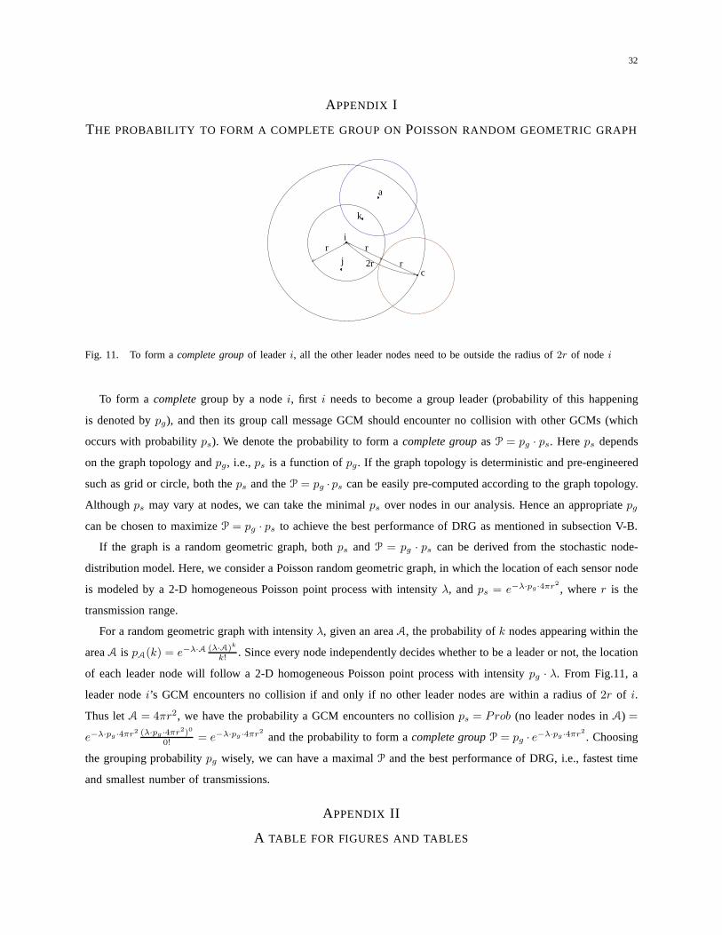
Fig. 11. To form acomplete group of leaderi, all the other leader nodes need to be outside the radius of2r of nodei

To form a complete group by a nodei, first i needs to become a group leader (probability of this happening

is denoted bypg), and then its group call message GCM should encounter no collision with other GCMs (which

occurs with probabilityps). We denote the probability to form acomplete group asP = pg · ps. Hereps depends

on the graph topology andpg, i.e.,ps is a function ofpg. If the graph topology is deterministic and pre-engineered

such as grid or circle, both theps and theP = pg · ps can be easily pre-computed according to the graph topology.

Although ps may vary at nodes, we can take the minimalps over nodes in our analysis. Hence an appropriatepg

can be chosen to maximizeP = pg · ps to achieve the best performance of DRG as mentioned in subsection V-B.

If the graph is a random geometric graph, bothps and P = pg · ps can be derived from the stochastic node-

distribution model. Here, we consider a Poisson random geometric graph, in which the location of each sensor node

is modeled by a 2-D homogeneous Poisson point process with intensity λ, andps = e−λ·pg·4πr2

, wherer is the

transmission range.

For a random geometric graph with intensityλ, given an areaA, the probability ofk nodes appearing within the

areaA is pA(k) = e−λ·A (λ·A)k

k! . Since every node independently decides whether to be a leader or not, the location

of each leader node will follow a 2-D homogeneous Poisson point process with intensitypg · λ. From Fig.11, a

leader nodei’s GCM encounters no collision if and only if no other leader nodes are within a radius of2r of i.

Thus letA = 4πr2, we have the probability a GCM encounters no collisionps = Prob (no leader nodes inA) =

e−λ·pg·4πr2 (λ·pg·4πr2)0

0! = e−λ·pg·4πr2

and the probability to form acomplete group P = pg · e−λ·pg·4πr2

. Choosing

the grouping probabilitypg wisely, we can have a maximalP and the best performance of DRG, i.e., fastest time

and smallest number of transmissions.

APPENDIX II

A TABLE FOR FIGURES AND TABLES

33

TABLE II

THE TABLE FOR FIGURES AND TABLES

Table I Algebraic connectivity on various graph topologies

Table II This table

Fig. 1. DRG Ave algorithm

Fig. 2. The collision among GCMs and the coverage of a group

Fig. 3. GraphG, the group cliques of each node and the auxiliary graphH

Fig. 4. The probability to form acomplete group v.s. the grouping probability

Fig. 5. The possible scenarios while running DRG Max onv

(0)

b and the minimum potential

Fig. 6. The instances of Poisson random geometric graph used in simulations

Fig. 7. The performance of DRG Ave on Grid and Poisson random geometric graphs

Fig. 8. An example that Flooding may never converge to correct average

Fig. 9. The comparison of the total number of transmissions of 3 distributed algorithms - DRG, Gossip, Flooding-m

Fig. 10. Uniform Gossip, Flooding, and Flooding-m

1 robust computation of aggregates in wireless sensor ... networks: distributed randomized...

Documents